of ghent robot - ghent...

University of Ghent Faculty of Engineering Sciences

Active Security of an Industrial Robot based on techniques of

Artificial Vision and Artificial Intelligence

by

Brecht FEVERY

Promotors:

Prof. Dr. Ir. José Ramón LLATA GARCÍA Prof. Dr. Ir. Luc BOULLART

Thesis presented to obtain the academic degree of Master in Electromechanical Engineering Sciences

Academic year 2006–2007

Gracias

José Ramón Llata, por darme esta oportunidad, por escucharme con paciencia, por enseñarme y motivarme.

Carlos Torre,

por la ayuda enorme en el campo de la visión.

David Castrillón, por la compañia de cada día en el laboratorio.

mis amigos Marco y Sarah, por los momentos de calidad.

Os olvidaré nunca.

Dankuwel

professor Boullart, voor de trouwe steun en

om een luisterend oor te zijn.

Dankjewel

mama en papa, voor het vertrouwen en

de steun tijdens al die jaren, om me te helpen praten en

naar me te luisteren, om me kansen zoals deze te geven.

broer Wouter,

voor je humor en om me te helpen ontspannen.

Stephane,

om er steeds te zijn op de weg die we samen aflegden.

Peter,

voor je frisse kijk op de zaken en je vriendschap in de voorbije 2 jaar.

Active Security of an Industrial Robot based on techniques of

Artificial Vision and Artificial Intelligence

by

Brecht FEVERY

[email protected]

Thesis presented to obtain the academic degree of

Master in Electromechanical Engineering Sciences

Santander, June 2007

Promotor of receiving university: Prof. Dr. Ir. José Ramón LLATA GARCÍA,

Universidad de Cantabria, E.T.S. de Ingenieros Industriales y de Telecomunicación,

Grupo de Ingeniería de Control,

Departamento de Tecnología Electrónica e Ingeniería de Sistemas y Automática (TEISA).

Promotor of home university: Prof. Dr. Ir. Luc BOULLART,

University of Ghent, Faculty of Engineering Sciences,

Department of Electrical Energy, Systems and Automation (EESA).

Abstract This Master’s Thesis proposes an active security system for the industrial FANUC Robot Arc Mate

100iB. The designed security system constitues of three fundamental components.

The first one is an artificial vision system that uses a set of network camera’s to watch the robot’s

workspace and instantaneously signals the presence of foreign objects to the robot. Stereoscopic

methods for pixel correspondences and 3D positional reconstructions are used to obtain the exact

obstacle’s location.

The second subsystem is an artificial intelligence system that is used to plan an alternative robot

trajectory in an on‐line manner. Fuzzy Logic principles were successfully applied to design a Fuzzy

Inference System that employes a rule base to simulate human reasoning in decision taking. The

Fuzzy Inference System generates translational and rotational actions that have to be undertaken

by the robot’s End Effector to avoid collision with the obstacle.

The third part of the active security system is a multitask oriented robot application written in the

KAREL programming language of FANUC Robotics, Inc. Upon detection of an obstacle, the motion

i

mailto:[email protected]

of a regular robot task is halted and motion along an alternative path is initiated and finished when

the original destination is reached.

The three subsystems of the active security system are connected by an overviewing real‐time

communication system. Socket connections between network devices are set up to exchange data

packages over Ethernet with the Transmission Control Protocol.

All subsystems of the active security system were tested, first seperately and then in an integrated

way. With special attention for real‐time performance, satisfying experimental results were

obtained.

Key words: Active Security, Artificial Intelligence, Artificial Vision, Fuzzy Logic, Obstacle

Avoidance, Real‐time, Robot Control.

ii

Index

Chapter 1. Introduction ………………………………………………………………… 1

1. Problem description ……………………………………………………………………………. 1

2. Real‐time considerations ………………………………………………………………………. 3

Chapter 2. Artificial Vision ……………………………………………………………. 5

1. Introduction ……………………………………………………………………………………… 5

2. Perspective projection methods ………………………………………………………………. 6

2.1 The pinhole camera model ……………………………………………………………. 6

2.2 Coordinate systems ……………………………………………………………………. 8

2.3 Correspondence between coordinate systems ………………………………………. 9

2.4 Perspective projection on the image plane…………………………………………… 11

2.5 Intrinsic and extrinsic camera parameters …………………………………………… 12

2.6 Modeling of projection errors due to lens distortion………………………………... 12

3. Camera calibration method and calibration results ………………………………………… 14

3.1 Calibration principles …………………………………………………………………….. 14

3.2 Calibration results…………………………………………………………………………. 16

4. Stereo vision methods to reconstruct three dimensional positions………………………… 19

4.1 Inversion of pixel distortion……………………………………………………………… 19

4.2 Calculation of the profundity ……………………………………………………………. 20

5. Pixel correspondence and object identification methods …………………………………… 22

5.1 Epipolar lines ……………………………………………………………………………… 22

5.1.1 Pixel equation of epipolar lines …………………………………………………… 24

5.1.2 Trinocular stereo algorithm based on epipolar lines …………………………… 26

5.2 Edge detection …………………………………………………………………………….. 28

5.2.1 Gradient operators …………………………………………………………………. 29

5.2.2 DroG operator………………………………………………………………………. 32

5.2.3 Canny operator ……………………………………………………………………... 33

5.3 Object identification algorithm ………………………………………………………….. 34

6. A real‐time camera implementation ………………………………………………………….. 35

6.1 Principles of camera image processing ………………………………………………… 36

6.2 Principles of the real‐time detection system …………………………………………… 37

6.3 Time evaluation of the vision system …………………………………………………… 40

iii

7. References ……………………………………………………………………………………….. 41

Chapter 3. Artificial Intelligence ……………………………………………………… 42

1.Introduction ……………………………………………………………………………………… 42

2. Design of a Fuzzy Inference System ………………………………………………………….. 43

2.1 Introduction ……………………………………………………………………………….. 43

2.2 Description of the avoidance problem …………………………………………………. 46

2.3 Basic philosophy of the avoidance strategy ……………………………………………. 48

2.4 Membership functions of the Fuzzy Inference System ………………………………. 54

2.4.1 Membership functions of entrance fuzzy sets …………………………………. 54

2.4.2 Membership functions of system outputs ………………………………………. 56

2.5 Construction of the rule base ……………………………………………………………. 58

2.5.1 Rules related to translational action ……………………………………………… 58

2.5.1.1 Repelling rules ………………………………………………………………. 58

2.5.1.2 Attracting rules ……………………………………………………………… 60

2.5.2 Rules related to rotational action ………………………………………………… 60

2.5.3 Continuity of the rule base ……………………………………………………….. 62

2.5.4 Consistency of the rule base …………………………………………………….... 62

2.6 The fuzzy inference mechanism ………………………………………………………… 63

2.6.1 Resolution of rule premises ………………………………………………………. 64

2.6.2 Implication of rule premises on rule consequents ……………………………… 64

2.6.3 Aggregation of rule consequents …………………………………………………. 65

2.7 Defuzzification process ………………………………………………………………….. 65

2.8 Algorithm of the Fuzzy Inference System ……………………………………………… 66

2.9 Real‐time performance of the Fuzzy Inference System ………………………………. 66

2.9.1 Time consumption of the Fuzzy Inference system……………………………… 67

2.9.2 Size of the distance increments and decrements ……………………………….. 67

2.9.3 Communication between the FIS and the robot controller ……………………. 69

3. References ……………………………………………………………………………………….. 70

Chapter 4. Active Security ……………………………………………………………… 71

1. Introduction …………………………………………………………………………………….. 71

2. FANUC Robot Arc Mate 100iB ………………………………………………………………... 72

2.1 Basic principles of motion manipulations ……………………………………………… 72

iv

2.2 Defining a user and tool coordinate system …………………………………………… 73

2.3 Memory space of the controller …………………………………………………………. 74

2.3.1 Flash Programmable Read Only Memory (FROM) .…………………………. 74

2.3.2 Dynamic Random Access Memory (DRAM) …………………………………. 75

2.3.3 Battery‐backed static/random access memory (SRAM)……………………… 75

2.3.4 Memory back‐ups ……………………………………………………………….. 75

3. KAREL programming ………………………………………………………………………….. 75

3.1 Programming principles …………………………………………………………………. 76

3.2 Program structure ………………………………………………………………………… 76

3.2.1 Variable declarations ……………………………………………………………. 76

3.2.2 Routine declarations …………………………………………………………….. 77

3.2.3 Executable statements …………………………………………………………… 77

3.3 Condition handlers ……………………………………………………………………….. 78

3.3.1 Basic principles…………………………………………………………………… 78

3.3.2 Condition handler conditions ………………………………………………….. 78

3.3.3. Condition handler actions ……………………………………………………… 79

3.4 Motion related programming features …………………………………………………. 79

3.4.1 Positional and motion data types ……………………………………………… 79

3.4.2 Position related operators ………………………………………………………. 80

3.4.3 Coordinate frames ………………………………………………………………. 80

3.4.4 Motion instructions ……………………………………………………………… 81

3.4.5 Motion types ……………………………………………………………………... 82

3.4.6 Termination types ………………………………………………………………. 83

3.4.7 Motion clauses …………………………………………………………………… 84

3.5 Read and write operations ………………………………………………………………. 86

3.5.1 File variables …………………………………………………………………….. 86

3.5.2 File operations …………………………………………………………………… 86

3.5.3 Input/output buffer ……………………………………………………………… 87

3.5.4 Example: reading in an array of XYZWPR variables ………………………… 87

3.6 Multi‐tasking ……………………………………………………………………………… 87

3.6.1 Task scheduling …………………………………………….…………………… 88

3.6.1.1 Priority scheduling ………………………………….…………………. 88

3.6.1.2 Time slicing ……………………………………………………………… 89

3.6.2 Parent and child tasks …………………………………………………………… 89

v

3.6.3 Semaphores ………………………………………………………………………. 89

3.6.3.1 Basic principles of semaphores ……………………………………….. 90

3.6.3.1.1 Wait operation ………………………………………………… 90

3.6.3.1.2 Signal operation ………………………………………………. 90

3.6.4 Motion control …………………………………………………………………… 92

4. Real‐time communication ……………………………………………………………………… 92

4.1 Full duplex Ethernet ……………………………………………………………………… 94

4.2 Fast Ethernet switches …………………………………………………………………… 94

4.3 Socket messaging …………………………………………………………………………. 96

4.3.1 KAREL socket messaging option ……………………………………………… 97

4.3.2 Socket messaging and MATLAB…………………………………………………. 98

4.3.3 Format of data packages ………………………………………………………… 99

4.3.4 KAREL communication program comm.kl …………………………………… 101

4.4 Real‐time performance of the Ethernet communication ……………………………… 102

5. The active security problem …………………………………………………………………… 103

5.1 A solution in KAREL……………………………………………………………………… 103

5.1.1 Secure.kl…………………………………………………………………………… 104

5.1.2 Moves.kl ………………………………………………………………………….. 104

5.1.3 Comm.kl ………………………………………………………………………….. 104

5.1.4 Task priorities ……………………………………………………………………. 105

5.1.5 Semaphore use and program execution dynamics…………………………… 106

6. Experimental results …………………………………………………………………………… 109

7. Acknowledgments ……………………………………………………………………………… 110

8. References ……………………………………………………………………………………….. 110

Chapter 5. Conclusion ..………….................................................................................... 112

Appendix A ………………………………………………………………………………. A.1

Appendix B ……………………………………………………………………………….. B.1

Appendix C ………………………………………………………………………………. C.1

vi

Chapter 1 Introduction 1. Problem description Robots have been successfully introduced in industry to automate production tasks of diverse

nature. Industrial robots work with expensive tools, on valuable products and at high speeds.

Often, a set of robots is working together on the same object to finish an assembly task in less

time. Nowadays, production cycles are refreshed at high rates and new robot applications need

to be programmed in short space of time. The use of sensors increases and the time to test new

applications decreases as production processes cannot be halted for long time. Collisions of

cooperating robots occur and when they do, they often cause damage to the robots and their

tools. Production processes then need to be stopped, reviewed and reinitiated.

From this point of view, the design of appropriate control systems that prevent collisions

between cooperating robots is of high economical importance. During the last years, the robot

industry and investigation centers have been strongly cooperating to design collision

avoidance software for use by industrial robots. Establishing collision free robot interaction,

without the need of rigid communication procedures between the involved robots, is identified

as a problem of active security.

From a non commercial point of view, robot active security can also be seen as guaranteeing

maximum safety to the human operator that is working close to an industrial robot. Especially

when working with heavy payloads and moving at high speeds, a robot arm hitting a human

operator can cause severe and even mortal injuries. Robot motion is often guided or controlled

by sensor information, but the trajectory along which the robot moves depends in the first place

on what has been programmed by the operator. Therefore, when a robot is executing a

programmed task, security precautions have to be taken at all times. Typically, robots operate

in an industrial work cell that is equipped with a security fence and sensors to detect when a

human operator is entering the workspace while the robot is executing its task. All active robot

motion will immediately be halted when a foreign object, e.g. a human operator, is detected by

the installed sensor system. In an active security system, upon detection of foreign objects,

robot motion would not be halted. An intelligent operating system would be activated to

assure the robot can continue executing its task. Motion would no longer take place along the

programmed trajectory, but along an alternative path that assures collision free motion. For a

simple manipulation task that consists of moving a part from where it has been detected to a

Chapter 1. Introduction

1_

predetermined final destination, this active security problem can be stated as the search for an

alternative path from an initial to the final destination, hereby moving around or above the

signaled obstacle.

The goal of this Master’s Thesis is to develop an active security system for the industrial

FANUC Robot Arc Mate 100iB, presented in figure 1.1. We will focus on the field of active

security where one robot has to continue collision free motion when an obstacle is encountered

in its workspace.

Figure 1.1: FANUC Robot Arc Mate 100iB

The foundations of the designed active security system are formed by artificial vision and

artificial intelligence systems.

An artificial vision system is able to derive from two dimensional camera images useful three

dimensional information about a camera covered area. The vision system that will be presented

in this thesis consists of a triplet of cameras that supplies information about the workspace’s

current setting. A thorough study of stereoscopic vision techniques was performed to design a

vision system that is able to detect foreign objects in the robots workspace. In chapter 2 we

present the theory about perspective projection methods, camera calibration issues, three

dimensional position reconstructions and object identification techniques.

Active security systems require the need of intelligent decision taking. Considering the current

position of the robot’s Tool Center Point, an alternative path has to be generated by taking


2_

logically derived actions. A system that simulates intelligent reasoning after it was trained by a

human programmer, is an artificial intelligence system. Out of the large set of artificial

intelligence techniques, we chose fuzzy logic. In chapter 3, the basic principles of fuzzy logic

will be elaborated. We will show how human reasoning can be simulated through the

introduction of linguistic distance descriptions and a rule base that constitutes of if‐then

implications.

After the design and testing of the artificial vision and intelligence systems, a robot active

security application was developed. Upon detection of an obstacle by the artificial vision

system, a normal execution task is interrupted. Execution priority is then passed to a security

task that makes the robot move along an alternative path calculated for with the artificial

intelligence system. A real‐time solution to this problem was implemented in the KAREL

programming language of Fanuc Robotics. In chapter 4 we will concentrate on the setup of a

communication between the robot controller and a pc, and on the programmed robot

application for which multitasking and semaphore principles will be introduced and used.

As this project has been the first one on the FANUC Robot Arc Mate 100iB of the research

group TEISA, a lot of primary research was performed to set up the robot control. A

communication protocol using Ethernet sockets was configured and KAREL programs for

motion manipulation were written, compiled and executed. To assure that this thesis can serve

as a basis for future research work, some practical aspects of the Fanuc robot and KAREL

programming issues will be also highlighted in chapter 4.

The goal of this thesis can be stated as the primary research in methodologies of artificial vision,

artificial intelligence and robot control. Since the principles of the methodologies and the

thorough understanding of concepts are more important than industrial performance, no

significant importance will be given to motion speed of the robot arm. Nevertheless, the

possibility to apply the design in real industrial applications will never be lost out of sight.

2. Real‐time considerations Since the previously described problem requires the processing of camera images, trajectory

planning and communication between a pc and the robot controller, one can intuitively

understand that we are dealing with a real‐time problem. Let us therefore focus on the meaning

of the term real‐time.

We can best situate the idea of real‐time systems by giving a few examples. A real‐time system

needs to react to stimuli within a time that is acceptable for the environment. For example, a

robot that is moving at high speed has to react quickly to external stop signals.


3_

In real‐time systems, a computer has to be able to receive and, if necessary, process data at the

same rate at which the data are produced. For example, when a vision system is installed to

detect obstacles in camera views, the operations needed to perform the detection action have to

be completed within the frequency of the image refreshment. When using multiple camera

views of a moving object, fast consecutive picture grabbing is necessary to assure the smallest

time interval possible between the registrations of the different images.

During our investigation work, real‐time performance has been one of our top priorities. A lot

of efforts were done to assure a high‐speed image transfer between the cameras and our matlab

sessions and to assure a fast communication between the robot‐controller and a pc. Time

performance was also important in the design of our artificial intelligence system, since the

time consumption for calculating positions along an alternative path is considerable. The

environmental factor that determines the real‐time performance of the artificial intelligence

system and the installed communication system is the speed of robot motion; a new position

needs to be calculated and transmitted to the robot controller before the previous position is

reached.

At the closure of chapter 2 and chapter 3, special attention will be given to the real‐time aspect

of the design. In chapter 4 that treats of robot control issues, the real‐time aspect is considered

in the parts about communication and multitasking.

3. References

[1] Real‐time and communication issues, M. G. Rodd, University of Swansea, Wales, UK, 1990.

[2] Multitasking & Concurrente Processen in Ware‐Tijd, Prof. dr. ir L. Boullart, Vakgroep

Elektrische Energie, Systemen & Automatisering, Faculteit Ingenieurswetenschappen,

Universiteit Gent.


4_

Chapter 2 Artificial Vision 1. Introduction

Determining accurately the three dimensional position of objects in the robot’s workspace is an

important first step in this project. In this chapter it will be described how three dimensional

positions of objects can be obtained using information of three vision cameras that cover the

entire workspace of the robot and hereby form an artificial vision system.

Stereo vision methods will be introduced to identify an object and to detect its position using

three images of the robot’s environment, taken in the same moment with the vision cameras.

The first step in the overall vision method is the identification of an object in a camera image.

This can be done focusing on specific characteristics of the object we want to detect. The

detection of a desk is an example of an identification problem that is relatively easy to solve, for

a desk is characterized by its rectangular surfaces which allow edge and corner detection. Both

of these techniques will be commented in this chapter.

The second step in the vision method is searching the correspondence between specific image

points in the three different images. In the example of the desk, solving of the correspondence

problem consists of determining the pixel coordinates of the corresponding desk corners in each

one of three images. In general, to solve the correspondence problem, geometric restrictions in

image pairs or triplets are used. The construction of conjugated epipolar lines in image planes

is a powerful restriction method that will be introduced in this chapter.

As we intuitively understand, a two dimensional camera image does not longer contain the

three dimensional information that fully describes an object in space, for the image has lost the

profundity information. However, once the corresponding image points have been detected in

a pair or triplet of images, the profundity information can be calculated. This third and final

step in the vision method will allow us to fully reconstruct the exact three dimensional position

of a detected object. A profundity calculation method based on the 2D information of a pair of

images will be introduced in this chapter.

To develop stereo vision methods, a step we cannot go without is the calibration process of the

vision cameras. This calibration procedure will provide us with the internal camera

characteristics such as focal length, position of the image’s principal point and distortion

coefficients that are used to model distortion of image coordinates due to lens imperfections.

These characteristics are called the intrinsic parameters of a camera. The calibration procedure

_ Chapter 2. Artificial Vision

5

also provides us with extrinsic parameters that consist of a rotation matrix and translation

vector that link the world reference coordinate system to the camera coordinate system.

2. Perspective projection methods In the following paragraphs it will be described how an object point, represented in a chosen

reference coordinate system, is projected into the image plane. A projection method according

to the pinhole model will be introduced. Besides the world reference coordinate system,

coordinate systems with respect to the camera and with respect to the image plane are

introduced and the transformations between these coordinate systems are described. Finally,

introducing the camera extrinsic and intrinsic parameters, a perspective projection method is

presented and a method to model projection errors due to lens distortion is proposed.

2.1 The pinhole camera model According to the pinhole model, each point P in the object space is projected by a straight

line through the optical center into the image plane. This projection model is represented in

figure 2.1a.

f

Z,z

Y,y

X,x

P (X,Y,Z)

p (x,y)

Optical center

Image plane

Figure 2.1a: The pinhole projection model

The determining parameter in this pinhole model is the focal distance f, that displays the

perpendicular distance between the optical center and the image plane. (X, Y, Z) represent

the three dimensional coordinates of P. The projection of P in the image plane is p with

coordinates (x, y).


6

In figure 2.1b, a two dimensional view of the pinhole projection model is displayed. The

optical center Oc lies at a distance f of the image plane π. The projection of Pc in the image

plane is Uc.

f

xc

zc

Image plane π

‐ fxc zc

Zc

Xc

Optical center Oc

Uc

Pc

Figure 2.1b: Coordinate correspondence in the pinhole model

Knowing the coordinates (xc, zc) of Pc in a camera coordinate frame (Xc, Yc, Zc) with origin

in Oc, we can obtain the x coordinate of Uc in the image plane by using the relations in

uniform triangles. Using an analogic drawing of the (Yc, Zc) plane for the y coordinate of Uc,

we can determine the relation between the (xc, yc, zc) coordinates of a point in space and the

coordinates (Ucx, Ucy) of its projection in the image plane:

c

ccy

c

ccx

zyfU

zxfU

⋅−=

⋅−= (2.1)

In this introduction of the pinhole camera model, we illustrated a transformation between

two coordinate systems: an Euclidean camera coordinate system (Xc, Yc, Zc) and an image

coordinate system in which the projected point Uc is presented. In perspective projection

methods, a number of different coordinate frames are typically used. In the next paragraph,

we will introduce the involved coordinate systems.


7

2.2 Coordinate systems The coordinate systems involved in perspective projection methods are represented in

figure 2.2.

Optical ray

Euclidean camera coordinate system

Focal point C

Optical axis

Zc

Xc

Yc

Object point P

Oc

Zw

Xw

Yw

Ow

R

T

Pw

Image plane π

wa

va

ua

Zi

Xi

Yi

fAffine image coordinate system

Euclidean image coordinate system

Principal point U0c=[0, 0, ‐f]T U0a=[u0, v0, 0]T

Pc

Oi

Euclidean reference coordinate system

Uc , u ~

Figure 2.2: Image projection related coordinate systems

The Euclidean world reference coordinate system is indicated with index w. The object

point P can be represented in these coordinates as Pw.

The Euclidean camera coordinate system –index c– has its z‐axis Zc aligned with the optical

axis, which is perpendicular to the image plane π. The origin of the camera coordinate

system is chosen coincident with the optical center Oc, which lies at a perpendicular

distance f to the image plane. The transformation between the world coordinate system and

the camera coordinate system is determined by a rotation vector R and a translation vector

T.


8

The Euclidean image coordinate system –index i– has its x‐ and y‐axis Xi and Yi in the

image plane. Axes Xi, Yi and Zi are parallel to the thosen camera coordinate system.

The fourth coordinate system is the affine image coordinate system –index a– in which

image points can be represented in Cartesian two dimensional coordinates. Using a scaling

factor that gives the number of image pixels per unit of length –mm in artificial vision

applications– we can express image points in pixel units. Axes va and wa are coincident

with Yi and Zi respectively, while ua has a different orientation than Xi. The main reason for

this is the fact that ua and va pixel axes may have a different scaling factor to represent

image points. This will be taken into account further on in the calibration parameter su (see

paragraph 3). Furthermore, in general pixel axes don’t have to be perpendicular, although

nowadays most camera types provide images with rectangular pixels.

The world reference system OwXwYwZw will be selected arbitrary in one certain calibration

image, where the reference system is fixed to the calibration pattern that we use when

executing the calibration procedure. This calibration procedure will be explained further on

in paragraph 3.

The final coordinate system to introduce is the reference coordinate system of the robot, to

which the robot controller refers all Tool Center Point positions and End Effector

orientations. The 3 point teaching method supported by the operational system of the

FANUC Robot Arc Mate 100iB allows the user the generate a so called UFRAME or user

coordinate frame. We taught a user coordinate frame that coincides with the reference

frame attached by the calibration method to one of the images of the calibration pattern.

This choice avoids the introducing of an extra transformation, because the vision reference

coordinate system coincides with the taught robot reference frame.

2.3 Correspondence between coordinate systems To express the object point P in the camera coordinate system, we have to rotate Pw using

the matrix R and than translate it along the vector T, as described by equation (2.2):

TPRP wc +⋅= , with and (2.2)

⎥⎥⎥

⎦

⎤

⎢⎢⎢

⎣

⎡=

w

w

w

w

zyx

P⎥⎥⎥

⎦

⎤

⎢⎢⎢

⎣

⎡=

c

c

c

c

zyx

P

Pc will now be projected into the image plane π along the optical ray that crosses the optical

center Oc. The result is Uc, expressed in Euclidean image coordinates. As we assumed the


9

projection according to the pinhole model, the coordinates of Uc will be given by equation

(2.3):

⎥⎥⎥⎥⎥⎥

⎦

⎤

⎢⎢⎢⎢⎢⎢

⎣

⎡

−

⋅−

⋅−

=⎥⎥⎥

⎦

⎤

⎢⎢⎢

⎣

⎡=

fz

yfz

xf

wvu

Uc

c

c

c

i

i

i

c (2.3)

The x‐and y coordinates of Uc were already obtained in equation (2.1). The value of the z‐

coordinate of Uc is identified by remarking that the optical axis is collinear with Zc and

perpendicular to the image plane π. The perpendicular distance is equal to the focal

distance f.

We can now compose an affine transformation to express the projected point Uc in the two

dimensional image plane, using homogeneous pixel coordinates: [ ]Tiii wvu ~~~ . The

transformation is given by a 3x3 matrix, applied as in equation (2.4). The factors a, b and c

can be interpreted as scaling factors along the axes of the Euclidean image coordinate

system. The third column can be seen as a translation along a vector containing the

negation of the coordinates of the image center point. In the image plane, the origin of the

coordinate system is often represented in the upper left corner. Therefore, substraction of

the principal point, U0a in figure 2, is needed to obtain a correct representation of points in

the image plane.

⎥⎥⎥⎥⎥⎥⎥

⎦

⎤

⎢⎢⎢⎢⎢⎢⎢

⎣

⎡

⋅−

⋅−

⋅⎥⎥⎥

⎦

⎤

⎢⎢⎢

⎣

⎡−−

=⎥⎥⎥

⎦

⎤

⎢⎢⎢

⎣

⎡

1

1000

~~~

0

0

c

c

c

c

i

i

i

zyf

zxf

vcuba

wvu

(2.4)

As we are working in homogeneous coordinates, we can manipulate equation (2.4),

multiplying by zc and repositioning the focal length f:


10

⎥⎥⎥⎥⎥⎥⎥⎥

⎦

⎤

⎢⎢⎢⎢⎢⎢⎢⎢

⎣

⎡

⋅⎥⎥⎥

⎦

⎤

⎢⎢⎢

⎣

⎡−⋅−−⋅−⋅−

⋅=⎥⎥⎥

⎦

⎤

⎢⎢⎢

⎣

⎡⋅

1100

0~~~

0

0

c

c

c

c

c

i

i

i

c zyzx

vcfubfaf

zwvu

z

⇔

⎥⎥⎥

⎦

⎤

⎢⎢⎢

⎣

⎡⋅=

⎥⎥⎥

⎦

⎤

⎢⎢⎢

⎣

⎡

c

c

c

i

i

i

zyx

Kwvu

~~~

(2.5)

The vector u~ represents the two dimensional homogeneous pixel coordinates of the image

point. We define the matrix K as:

⎥⎥⎥

⎦

⎤

⎢⎢⎢

⎣

⎡−⋅−−⋅−⋅−

=100

0 0

0

vcfubfaf

K (2.6)

We call the matrix K the calibration matrix of the camera, for it contains the information we

will later on obtain from the calibration process.

2.4 Perspective projection on the image plane Based on the constructed coordinate transformations we can now compose a direct and

open form transformation between the world reference coordinate system and the affine

image coordinate system. Let wP~ be the homogeneous coordinates of the object point P in

the reference coordinate system:

[ ]T

ww PP 1~ = (2.7)

Knowing that wP~ can be transformed to the camera coordinate system by applying a

rotation and a translation according to equation (2.2), we can recombine (2.5) to obtain the

following transformation:

[ ] ww

i

i

i

PMP

TKRKwvu

~1~

~~

⋅=⎥⎦

⎤⎢⎣

⎡⋅⋅⋅=

⎥⎥⎥

⎦

⎤

⎢⎢⎢

⎣

⎡ (2.8)


11

We define M as the projection matrix of the camera system. M is a 3x4 matrix consisting of

two sub matrices:

• The first 3x3 part describing a rotation

• The right 3x1 column vector representing a translation.

The knowledge of projection matrix M allows us to project any arbitrary object point in the

reference system into the image plane, resulting in the two dimensional Cartesian

coordinates of this image point. The numerical form of M will proof to be absolutely

necessary in the hour of reconstructing three dimensional positions of objects out of the 2D

information of two images taken in the same moment by two different cameras of our

artificial vision system.

2.5 Intrinsic and extrinsic camera parameters

Intrinsic camera parameters are the internal characteristics of a camera. Without taking into

account projection errors due to lens distortion, they describe how object points expressed

in the camera reference system are projected into the image plane, according to equation

(2.5). We identify the intrinsic parameters as the focal length f and the principal point

(u0, v0), that marks the center of the image plane. Both values can differ considerably from

theoretical values and therefore an accurate camera calibration is absolutely necessary.

These parameters describe a specific camera and are independent of the camera’s position

and orientation in space.

The extrinsic parameters of a camera do depend of the camera’s position and orientation in

space, for they describe the relationship between the chosen world reference coordinate

system and the camera reference system. These parameters are given by the rotation matrix

R and translation vector T mentioned above. R contains the 3 elementary rotations that are

to be executed in order to let the axes of the reference frame align with the axes of the

camera coordinate system, while T represents the translation from the origin of the

reference system to the camera system.

The calibration matrix K has the intrinsic camera parameters as its components. The

projection matrix M consists of both intrinsic and extrinsic camera parameters.

2.6 Modeling of projection errors due to lens distortion The presented pinhole projection model is only an approximation of a real camera model

because distortion of image coordinates due to imperfect lens manufacturing is not taken


12

into account. When high accuracy is required, a more comprehensive camera model can be

used that describes the systematical distortion of image coordinates. A first imperfection in

lens manufacturing is the radial lens distortion that causes the actual image point to be

displaced radially in the image plane [3]. In their paper on camera calibration, Heikkilä and

Silvén propose an approximation of the radial distortion according to expression (2.9).

⎥⎦

⎤⎢⎣

⎡

++++

=⎥⎦

⎤⎢⎣

⎡

...)(

...)(4

22

1

42

21

)(

)(

iii

iiir

i

ri

rkrkvrkrku

vu

δδ (2.9)

where the superscript (r) indicates radial distortion, k1, k2,… are coefficients for radial

distortion and 22iii vur += . The coordinates ui and vi are the first two coordinates of the

projected object point in Euclidean image coordinates Uc, according to equation (2.3).

Typically, one or two coefficients are enough to compensate for radial distortion [3], and

that is the number of radial distortion coefficients we are going to apply in our camera

model.

As a second imperfection, centers of curvature of lens surfaces are not always strictly

collinear. This introduces another common distortion type, decentering distortion, which

has both a radial and a tangential component [3]. The expression for the tangential

distortion proposed by Heikkilä is written in the form of expression (2.10).

⎥⎦

⎤⎢⎣

⎡

++++

=⎥⎦

⎤⎢⎣

⎡

iiii

iiiit

i

ti

vupvrpurpvup

vu

222

1

2221

)(

)(

2)2()2(2

δδ (2.10)

where the superscript (t) indicates tangential distortion and p1 and p2 are coefficients for

tangential distortion.

Once the distortion terms are defined, a more accurate camera model can be introduced.

Based on the general projection transformation (2.4), Heikkilä proposes a camera model

given by expression (2.11).

⎥⎦

⎤⎢⎣

⎡+⎥

⎦

⎤⎢⎣

⎡

++++

=⎥⎦

⎤⎢⎣

⎡′′

0

0)()(

)()(

)()(

~~

vu

vvvDuuusD

vu

ti

riiv

ti

riiuu

i

i

δδδδ (2.11)

The distorted image point [ ]T

ii vu ′′ ~~ is expressed in homogeneous pixel coordinates. We

recognize the radial and tangential distortion terms and the referencing of image points to

the principal point (u0, v0). As for the set of original scaling factors a, b and c we can see that

b is taken equal to zero –implying orthogonal pixel axes– and a and c are represented by


13

one scaling factor su along the u pixel axis. Du and Dv indicate the number of pixels per unit

of length in u and v pixel direction respectively.

This camera model will be used in the calibration procedure that will be commented in the

next paragraph. The set of introduced distortion coefficients will have to be estimated

during the calibration process, together with the intrinsic parameters focal length f,

principal point (u0, v0) and scaling factor su along the u pixel axis. Du and Dv are given

camera characteristics that can be obtained from the known image size in pixels, for

example 640x480, and the sensor’s chip size expressed in units of length.

3. Camera calibration method and calibration results By executing a geometrical camera calibration we can determine the set of camera parameters

that describe the mapping between 3D reference coordinates and 2D image coordinates.

Various methods for camera calibration can be found from literature. A very accurate method

is presented in the paper A Four‐step Camera Calibration Procedure with Implicit Image Correction

[3], written by Janne Heikkilä and Olli Silvén. The method consists of a four‐step procedure

that uses explicit calibration methods for mapping 3D coordinates to image coordinates and an

implicit approach for image correction.

A calibration of our camera system is executed using a MATLAB camera calibration toolbox that

is based on the calibration principles introduced in [3]. The mentioned MATLAB toolbox is freely

available on the internet [4]. In this paragraph the basic principles of the performed calibration

will be briefly exposed. For a thorough explanation of the calibration steps, the original

Heikkilä publication can be consulted.

3.1 Calibration principles


14

]

In the first calibration step, the basic intrinsic parameters focal length f and principal point

(u0, v0) are calculated in a non‐iterative, least squares fashion ignoring the nonlinear radial

and tangential pixel distortion. The scaling factor su is assumed to be 1. For a number of N

control points we can write down the linear transformation between Euclidean camera

coordinates (xc, yc, zc) and homogeneous image pixel coordinates [ Tiii wvu ~~~ , according

to equation (2.8):

w

i

i

i

PMwvu

~

~~~

⋅=⎥⎥⎥

⎦

⎤

⎢⎢⎢

⎣

⎡ (2.8)

The projection matrix M is unknown and contains the intrinsic parameters in an implicit,

closed form. Knowing the image and reference coordinates of a selected set of N grid

points, we can construct a set of 2xN equations with the 12 elements of M as unknown

values [3]. Using constraints proposed in [3], this over determined set of equations can be

solved for the 12 elements of M. A technique to decompose matrix M into a subset of

matrices containing f and (u0, v0) in a direct way is presented. Using the software, the set of

N control points is created by indicating manually the four extreme grid corners of the

calibration pattern in every picture. The used calibration pattern has the form of a checker

board with white and black adjacent squares of fixed and equal dimension. In order to

reconstruct the position of all grid corners, the square size has to be entered as a function

variable.

No iterations are required for this first direct and linear method. However, lens distortion

effects can not be incorporated. Therefore, a nonlinear parameter estimation is introduced

in the second calibration step that incorporates lens distortion. In [3], it is suggested to

estimate the camera parameters simultaneously minimizing the residual between the

model (distorted pixel coordinates [ ]Tii vu ′′ ~~ ) and N observations [ . The function F

to minimize is then expressed as a sum of squared residuals:

]Tii VU

∑∑==

′−+′−=N

iii

N

iii vVuUF

1

2

1

2 )~()~( (2.12)

Since estimation occurs simultaneously, this method involves an iterative algorithm. As

initial parameter values, the parameters obtained from the direct linear method are used. In

this model we use the projection model presented before in equations (2.10) and (2.11).

Execution of the iteration results in 8 intrinsic parameters: f, (u0, v0), k1, k2, p1, p2 and su.

Perspective projection is generally not a shape preserving transformation. Two‐ and three‐

dimensional objects with a non‐zero projection area are distorted if they are not coplanar

with the image plane [3]. Heikkilä and Silvén present a third calibration step to compensate

for this perspective projection distortion by calculating a distortion formula for the pixel

coordinates. The distortion formula and coefficients are elaborated based on considerations

for distortion of circular objects, that tend to be depicted in the image plane as ellipses,

depending on the angle and displacement between the object surface and the image plane.

In the fourth step of their calibration procedure, Heikkilä and Silvén present how the

distortion of the pixel coordinates can be undone. This is a very important step in the


15

inverse mapping problem that will be presented in paragraph 4 of this chapter. We will

explain the principle of undoing the pixel distortion in that paragraph further on.

Applying the calibration procedure provided in the MATLAB toolbox, we use calibration

patterns as described before. These patterns are printed and fixed to a flat, coplanar

structure, e.g. a wooden board. The fact that the scheme of calibration points is coplanar

introduces a singularity and causes the number of parameters that can be estimated from a

single view to be limited [3]. Therefore, multiple views are required in order to solve all the

intrinsic parameters. Typically, a set of 20 pictures of the calibration pattern, in different

positions with respect to the camera, is used. A reference coordinate system is fixed to the

pattern in each picture, by selecting the four most outer grid corners, as described before.

For each of these reference coordinate systems, a rotation matrix R and a translation vector

T, relating the reference system to the camera coordinate system, will be calculated during

the calibration procedure. As a result of the execution of the calibration functions we get

the set of 8 calibration parameters and as many sets of extrinsic camera parameters (matrix

R and vector T) as there are pictures and thus reference frames.

3.2 Calibration results The cameras of our vision system are Axis205 networks cameras. The optical characteristics

of these cameras are provided by the fabricant:

nominal focal length = 4 mm

effective CCD chip size = 0,25 inch

The nominal focal length is a theoretic value. The effective focal length of all cameras will

in practice slightly differ from the nominal focal length. It can only be obtained through

camera calibration and will also differ from one camera to another. This is due to the

unique lens manufacturing of every camera.

The effective CCD chip size is given as the diagonal distance of the rectangular chip and is

assumed to be equal for all cameras. We need the value of this characteristic to obtain the

conversion rate between pixel units and length units. These conversion rates are

determined by firstly calculating the effective CCD chip size in horizontal and vertical

direction and then dividing these chip sizes by the number of image pixels in horizontal,

respectively vertical direction. The resolution of the images worked with in our vision

system is 480x640 pixels. Denoting the conversion rate in horizontal direction as Du and the

conversion rate in vertical direction as Dv, we obtain for our vision cameras the values _ Chapter 2. Artificial Vision

16

according to table 2.1. As can be seen, camera resolutions are chosen in a way that allows

us to work with equal conversion rates in horizontal and vertical pixel direction.

Du [pixels/mm] Dv [pixels/mm]

125,98 125,98

Table 2.1

From the calibration process we obtain two sets of camera parameters. The first set consists

of the intrinsic camera parameters: effective focal length f, scaling factor su along the u pixel

axis, image center point (u0, v0), radial distortion coefficients p1 and p2 and the tangential

distortion coefficients k1 and k2. For each one of the three calibrated cameras, this set of

intrinsic parameters is indicated in table 2.2. These parameters are stated in conformity

with the formulations of Heikkilä. For the reader who is planning to use the MATLAB

camera calibration toolbox, we mention that the Heikkilä parameters differ from the output

of the toolbox. Conversion conventions can be found on the camera calibration webpage [4].

Camera 1 Camera 2 Camera 3

f 5.5899 mm 5.574 mm 5.6109 mm

su 1.0001 1.0012 0.9989

(u0, v0) (354, 203) (355, 244) (359, 262)

p1 ‐2.5476 x 10‐3 ‐2.5554 x 10‐3 ‐2.5227 x 10‐3

p2 4.325 x 10‐5 4.367 x 10‐5 4.3771 x 10‐5

k1 ‐4.1428 x 10‐5 ‐1.1523 x 10‐4 ‐8.3651 x 10‐5

k2 ‐3.4789 x 10‐5 ‐6.2488 x 10‐5 ‐1.4069 x 10‐4

Table 2.2

To give the reader an idea of the mentioned pixel coordinates displacements due to lens

imperfections, the typical view of pixel distortions is represented in figures 2.3 and 2.4.

Figure 2.3 displays the radial distortions. The arrows indicate the magnitude of the radial

displacements in pixel units.


17

Figure 2.3: Visualisation of radial distortion components

Figure 2.4: Visualisation of tangential distortion components

The arrows in figure 2.4 indicated how pixels are deformed due to tangential distortions.

The tangential character can be identified from the tangential direction of the arrows in the

upper right and the lower left corner of figure 2.4.

In both figures, the displacement of the image center point (u0, v0) away from the theoretic

center point (240, 320) is depicted. The calculated and theoretic center points are

represented as a circular spot and cross respectively.


18

4. Stereo vision methods to reconstruct three dimensional positions Once the calibration of a camera is performed, the perspective projection of a camera system is

fully determined, for the projection matrix M can be constructed using intrinsic and extrinsic

camera parameters. However, the projection of object points is not what we intend. What we

aim to do is reconstructing three dimensional positions. This problem is denoted as the inverse

mapping. We start from known image pixel coordinates, which tend to be distorted due to lens

imperfections. In a first step of the inverse mapping, pixel coordinates will have to be

undistorted. Next, calculation of the lost profundity in 2D pictures can be realized once we

have two or three sets of corrected pixel coordinates of corresponding image points.

To obtain the corresponding pixel sets, an object first has to be detected in a pair or triplet of

camera images taken in the same moment by different calibrated cameras. In the next

paragraph, we will focus on the identification of objects in images and on methods to

determine the correspondence between characteristic pixels in different images.

Not considering the prior step of searching for pixel correspondences, we can separate the

inverse mapping of pixel coordinates to reference frame coordinates into two sub problems:

• Undoing distortion of pixel coordinates

• Calculation of the profundity

4.1 Inversion of pixel distortion


19

]As can be seen from the projection model (2.11), the expressions for the distorted pixel

coordinates [ are fifth order nonlinear polynomials in uTii vu ′′ ~~ i and vi, the Euclidean image

coordinates. This implies that there is no explicit analytic solution to the inverse mapping,

when both radial and tangential distortion components are considered [3]. Heikkilä and

Silvén present an implicit method to recover the undistorted pixel coordinates [ ]Tii vu ~~ ,

knowing the distorted coordinates [ ]Tii vu ′′ ~~ starting from the physical camera parameters

obtained from the calibration process. With the results of the three calibration steps

described in paragraph 3.1, it is possible to solve for the unknown parameters of an inverse

model by generating a dense grid of NxN Euclidean image points and calculating

the corresponding distorted image coordinates

( ii vu )

( )ii vu ′′ ~~ by using the camera model (2.11).

Subsequently, an implicit inverse camera model, describing the distorted image

coordinates as a function of distorted Euclidean coordinates ( is introduced.

The parameters of this inverse model are then solved for iteratively using a least squares

( ii vu ′′ ~~ ) )ii vu ′′

technique. Typically, a set of 1000‐2000 created grid points, e.g. 40x40, is enough to obtain

satisfying results. For an extended explanation of this method, we refer to [3].

In our artificial vision application, pixel coordinates are undistorted using the MATLAB

functions invmodel and imcorr provided by Heikkilä. As entrance to invmodel we give the

intrinsic parameters that describe the projection model obtained by camera calibration. The

function invmodel then returns the parameters of an inverse camera model that can be used

to undistort pixel coordinates with the function imcorr. This function allows us to convert a

set of N pixel coordinates, entered as a Nx2 vector, which will support us in the hour of

online conversion of pixel coordinates.

4.2 Calculation of the profundity

A general case of image projection into an image plane is presented in picture 2.5. The same

object point P is projected into the image plane of a left and right positioned camera. These

two camera systems are fully identified by their projection matrices Ml and Mr of the left

and right camera respectively. The optical centers of both projection schemes are depicted

as Cl and Cr, while the projections of P in both image planes are pl and pr.

P(X,Y,Z)

Cl Cr

pl pr

Ml Mr

Figure 2.5: Object point projection in two image planes

According to the notations of equation (2.8) we can calculate the projections of the object

point P in the image planes:

PMp

PMp

rr

ll~~

~~

⋅=

⋅= ⇒ (2.13)

⎪⎪⎪⎪

⎩

⎪⎪⎪⎪

⎨

⎧

⋅⎥⎥⎥

⎦

⎤

⎢⎢⎢

⎣

⎡=

⎥⎥⎥

⎦

⎤

⎢⎢⎢

⎣

⎡

⋅⎥⎥⎥

⎦

⎤

⎢⎢⎢

⎣

⎡=

⎥⎥⎥

⎦

⎤

⎢⎢⎢

⎣

⎡

Pmmm

wvu

Pmmm

wvu

r

r

r

r

r

r

l

l

l

l

l

l

~

~~~

~

~~~

3

2

1

3

2

1


20

where mkl and mkr (k=1, 2, 3) are the rows of matrices Ml and Mr respectively.

Having the pixel coordinates of pl and pr as given, we can calculate the associated

homogeneous coordinates by taking into account a scaling factor α:

( ) ( )ααα ,,~~~

lllll vuwvu ⋅⋅= (2.14)

Equation (2.14) shows the homogeneous coordinates of pl. We can now rewrite equation

(2.13) for the left projection pl:

⎪⎩

⎪⎨

⎧

⋅=⋅=⋅⋅=⋅

PmPmuPmu

l

ll

ll

~~~

3

2

1

ααα

(2.15)

Substitution of the scaling factor α in the first two equations and rearranging terms gives us:

( )( )⎩

⎨⎧

=⋅−⋅⇒⋅=⋅⋅=⋅−⋅⇒⋅=⋅⋅

0~~~0~~~

2323

1313

PmmvPmvPmPmmuPmuPm

llllll

llllll (2.16)

For pr we can compose similar equations. Eventually we get:

(2.17) 0~~

23

13

23

13

=⋅=⋅

⎥⎥⎥⎥

⎦

⎤

⎢⎢⎢⎢

⎣

⎡

−⋅−⋅−⋅−⋅

PAP

mmvmmummvmmu

rrr

rrr

lll

lll

The solution P~ of this equation gives us the homogeneous coordinates of the three

dimensional object point in the world reference system:

⎥⎥⎥⎥

⎦

⎤

⎢⎢⎢⎢

⎣

⎡

⋅⋅⋅

=

⎥⎥⎥⎥⎥

⎦

⎤

⎢⎢⎢⎢⎢

⎣

⎡

=

αααα

αZYX

ZYX

P ~~~

~ (2.18)

We identify matrix A as a 4x4 matrix. The solution P~ of (2.17) is the one that minimizes the

squared distance norm 2~PA⋅ . The solution to this minimization problem can be identified

as the unit norm eigenvector of the matrix ( )AAT ⋅ , that corresponds to its smallest

eigenvalue [5].


21

Dividing the first three coordinates by the scaling factor, we obtain the Euclidean 3D

coordinates of the object point P:

⎥⎥⎥

⎦

⎤

⎢⎢⎢

⎣

⎡=

ZYX

P (2.19)

5. Pixel correspondence and object identification methods If a desk corner is detected in one image at location (u1, v1) in pixel coordinates, we need to find

out what pixel coordinates (u2, v2) in a second image correspond to the same desk corner. We

denominate this problem as the search for pixel correspondences. Before any 3D positional

reconstruction can be performed, the correspondence of characteristic image points has to be

searched for in all images involved in the reconstruction process. Typically, geometrical

restrictions in the considered image planes will be used. We will focus on epipolar lines, for

they form the key in the solution of many correspondence problems. We will introduce the

concept of epipolar lines and illustrate their power through the introduction of epipolar line

equations in pixel coordinates. A trinocular vision algorithm will be introduced to solve the

pixel correspondence problem.

Often used in combination with epipolar lines, specific detection methods are employed to

identify objects that have certain characteristics. E.g. an object that is constituted of clearly

separated surfaces will be easy to detect using edge detection methods. Because separated

surfaces are touched by the light in a different way, regions with different color intensity will

be displayed in the object’s image. Gradient operators are used to detect the transition between

regions with different pixel color intensity. The transition zones are denoted as the image edges

and can form the contours of an object to detect.

More advanced algorithms for characteristics detection, such as corner detection, exist and can

be found in image processing form as MATLAB functions on the support website of MATLAB[6].

At the end of this paragraph it will be explained how methods based on epipolar lines and

methods for image characteristics detection can be used in an integrated way to solve the

general object localization problem.

5.1 Epipolar lines The idea of epipolar lines can be explained looking at figure 2.6. The projection of an object

point P1 in the left image plane is denoted as pl. The projection line passes through the

optical center Cl. All points in space that lie on this projection line Clpl are projected onto _ Chapter 2. Artificial Vision

22

the same image point pl. P2 is an example of such a point in space. In the right image plane

the projection of P1 is denoted as pr1. The point P2, that had the same projection in the left

image plane as the point P1, is in the right plane however projected onto the image point pr2

that differs from pr1.

The epipolar line associated to the image point pl is now introduced as the projection in the

right image of the set of points in space that are projected through the optical center Cl of

the left image onto the image point pl. Analogically, the epipolar line associated to the

image point pr can be constructed. It can be seen in figure 2.6 that the construction of the

two epipolar lines associated to the point in space P1 fully symmetric.

P1

P2

Er El Cl

Cr

pl

pr2

pr1

π epipolar line associated to pr1 and pr2

epipolar line associated to pl

Figure 2.6: Epipolar lines principle

To the point P1 we can associate a plane, denominated epipolar plane, which is formed by

pl and the optical centers Cl and Cr. The epipolar plane intersects with the image planes

along both epipolar lines. All other points in space have associated epipolar planes that

also contain the line ClCr. This causes all epipolar lines of an image set to intersect in one

and the same point in each plane. These special points are denominated epipoles. The

epipoles drawn in figure 2.6 are denoted as El and Er for left and right image plane

respectively.

The geometric restriction based on epipolar geometry can now be stated in the following

sentence:

The image point pr in the right image that corresponds to the point pl in the left image has to be

situated on the epipolar line associated to pl.


23

In order to use this restriction in the design of a vision method, we will have to construct

the equations of epipolar lines. This equation will be introduced in the next paragraph.

After that, an algorithm based on epipolar lines will be introduced to solve pixel

correspondences in a trinocular vision algorithm.

5.1.1 Pixel equation of epipolar lines

A point P in the 3D space can be represented with respect to each of two camera coordinate

systems. The origins of the two image planes are the optical centers of the camera systems

and denoted in figure 2.7 as Cl and Cr. The vectors that connect P with Cl and Cr are

denoted as Pl and Pr respectively. One camera coordinate system can be transformed in the

other by applying a rotation and a translation. In the calibration procedure, we obtained

the extrinsic parameters of each camera system. Those extrinsic parameters described the

relation between each camera coordinate system and a chosen world reference system.

Since we know how to transform each camera frame into the reference frame, we can also

transform one camera frame into the other.

P1

Er El Cl

Cr

pl pr

π

Pl

Pr

Tc

Figure 2.7: Equation of epipolar lines

Let us denominate the rotation matrix of this transformation as Rc and the translation

vector as Tc = Cr – Cl. This way, the relation between Pr and Pl can be written as:

( )clcr TPRP −⋅= (2.21)

Applying perspective projection to Pl and Pr we obtain the image coordinates (in mm) of

the projected images points pl and pr:


24

(2.21)

⎪⎪⎩

⎪⎪⎨

⎧

⋅=

⋅=

r

rrr

l

lll

ZfPp

ZfPp

Let us consider the vectors Pl, Tc and Pl–Tc in the epipolar plane. Since the vectors Tc and Pl

are coplanar, the vector product lc PT × results in a vector perpendicular to the epipolar

plane. Therefore, the scalar product of Pl–Tc and lc PT × is zero. Taking into account

equation (2.21) we obtain:

( ) ( ) 0=×⋅⋅ lc

T

rT

c PTPR (2.22) We now introduce a matrix S so that ( ) lclc PTSPT ⋅=× :

( )⎥⎥⎥

⎦

⎤

⎢⎢⎢

⎣

⎡

−−

=0

00

xy

xz

yz

c

tttt

ttTS , with (2.23)

⎥⎥⎥

⎦

⎤

⎢⎢⎢

⎣

⎡=

z

y

x

c

ttt

T

Equation (2.22) can now be written as follows:

( ) 0=⋅⋅⋅ lcc

Tr PTSRP (2.24)

The points Pr and Pl in (2.24) are expressed in the camera coordinate system. In equation

(2.5) of paragraph 2.3, we composed an affine transformation between the camera reference

frame and the two dimensional image plane, using homogeneous pixel coordinates:

⎥⎥⎥

⎦

⎤

⎢⎢⎢

⎣

⎡⋅=

c

c

c

zyx

Ku~ where (2.5) ⎥⎥⎥

⎦

⎤

⎢⎢⎢

⎣

⎡=

c

c

c

c

zyx

P

Pc is a point in space expressed in camera coordinates (in mm) and K represents the matrix

containing the intrinsic camera calibration parameters. Using the inverse transformation

we can write the points Pr and Pl of equation (2.24) as follows:

⎩⎨⎧

⋅=⋅=

−

−

rrr

lll

pKPpKP~~

1

1

(2.25)


25

The respective pixel coordinates of Pl and Pr are denominated lp~ and rp~ . The calibration

matrix of left and right camera are denominated Kl and Kr respectively. Equation (2.24) can

now be written as:

( ) ( ) 0~~0~~1

11 =⋅⋅⇔=⋅⋅⋅⋅⋅ −−l

Trllcc

T

rT

r pFppKTSRKp (2.26)

where ( ) ( ) 111

−− ⋅⋅⋅= rcc

T

l KTSRKF (2.27)

The matrix F1 is called a fundamental matrix. In equation (2.26) lpF ~1 ⋅ can be considered as

the projection line in the right image plane that passes through pr and the epipole Er. If we

write the projection line lpF ~1 ⋅ as ru~ , equation (2.26) becomes:

0~~ =⋅ r

Tr up (2.28)

This is the equation of the epipolar line in the right image plane, associated to the

projection pl of a point P in space in the left image plane. Analogically, the equation of the

epipolar line in the left image associated to the projection pr in the right image can be

expressed as:

0~~ =⋅ ll up (2.29)

where rl pFu ~~2 ⋅= and ( ) ( ) 11

2−− ⋅⋅⋅= rcc

T

l KTSRKF (2.30) The fundamental matrices F1 and F2 define the relation between an image point, in left and

right image respectively, and its associated epipolar line in the conjugate image, expressed

in pixel coordinates. The construction of the epipolar line equation was taken from the

Master’s Thesis Reconstrucción de piezas en 3D mediante técnicas basadas en visión estereoscópica

by Carlos Torre Ferrero [5].

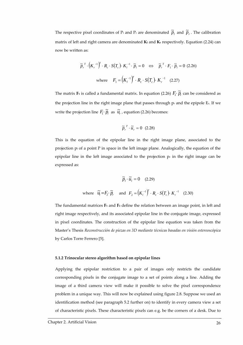
5.1.2 Trinocular stereo algorithm based on epipolar lines Applying the epipolar restriction to a pair of images only restricts the candidate

corresponding pixels in the conjugate image to a set of points along a line. Adding the

image of a third camera view will make it possible to solve the pixel correspondence

problem in a unique way. This will now be explained using figure 2.8. Suppose we used an

identification method (see paragraph 5.2 further on) to identify in every camera view a set

of characteristic pixels. These characteristic pixels can e.g. be the corners of a desk. Due to _ Chapter 2. Artificial Vision

26

imperfections in the corner detection method, pixels that actually don’t belong to the set of

corner pixels might have been detected. The goal of this algorithm is to obtain, for every

true corner pixel in the left image, the location of the corresponding two corner pixels in the

central and right image plane.

The designed method will now be explained for the pixel pl that lies in the left image plane

Il, and that is the projection of the object point P through the optical center Cl. The actual

corresponding projections in the right and central image plane Ir and Ic with optical centers

Cr and Cc are denoted pr and pc respectively.

. .

.

. . . .

.

Ic

CcIl

pl

Cl Cr

pr

Pr1

P(x, y, z) .

Prm

Rr

Rcpc

Rc1

Rcm

Rcj

Ir

Figure 2.8: Trinocular correspondence algorithm based on epipolar lines

Knowing the intrinsic and extrinsic parameters of the camera triplet, the epipolar lines

corresponding to the projection pl of P in the left image can be constructed in the right and

central image plane. These epipolar lines are denoted Rr and Rc for right and central image

plane respectively. In the right image plane we now consider the pixels that have been

previously detected as characteristic ones (e.g. possible desk corners pixels) and select

those that lie on the epipolar line Rr or sufficiently close to it. We can call these pixels the

candidate pixels of Ir and they are denoted in figure 2.8 as Pri, i=1…m.

In the central image plane we can now construct the epipolar lines that correspond to the

pixels Pri. This set of epipolar lines is denoted as {Rci, i=1…m}. The correct pixel

correspondence is now found by intersecting Rc with the epipolar lines of the set {Rci} and

selecting the central image pixel that lies on the intersection of Rc and a line Rcj in the set

{Rci}. Once this pixel is detected, the unique corresponding pixel triplet {pl, pc, pr} is found.


27

In practice, correspondent pixels will never lie perfectly on the intersection of the epipolar

lines constructed in the third image. Therefore, we have to define what pixel distance can

be considered as sufficiently small to conclude a pixel correspondence. The more, extra

attention has to be paid to the noise effect in images, which tends to promote the detection

of untrue characteristic pixels. In the ideal case, no pixel correspondence will be detected

for an untrue characteristic pixel, because it hasn’t been detected in the other images and its

epipolar line doesn’t come close to one of the true or untrue characteristic pixels in the

other images. If a correspondence does have been originated by one or more untrue

characteristic pixels, a correspondent pixel triplet will result at the end of the algorithm.

However, it will be able to discard the untrue correspondence after reconstructing its 3D

location, for most probable this 3D position will lie far from the 3D workspace in which

you supposed your object was to be detected.

5.2 Edge detection Edge detection is a powerful method that can be used to identify in camera images those

objects that have surfaces that are clearly separated in color, orientation or in both color

and orientation. Light effects on differently oriented surfaces or color differences will cause

adjacent image regions to possess significant differences in gray scale level. The image

edges are defined as the transition zones between two regions with significantly distinct

gray scale properties.

Because gray scale discontinuities have to be detected, the commonly used edge detection

operators are derivative operators. Typically, two derivative operators appear in literature.

The first one is the Gradient operator and is based on the first derivative. It looks for the

maximum gray scale transitions in an image. The second operator is the Laplace operator

and is based on the second derivative. It looks for zero crossings in the gray scale image. In

this introduction on edge detection we will focus on the Gradient operator, for this

operator forms the basis of the Canny operator applied on discrete images. The Canny

operator is the operator we will apply in our vision system to detect the edges of objects.

For a thorough explanation of the Laplace operator for edge detection, we refer to literature

[7].

In the detection of edges an important disturbance factor is image noise. This noise can be

caused by the subsequent processes of image capturing, digitalization of the image and its

subsequent transmission [7]. Filter operations on the discrete images are applied to reduce

this noise. We will introduce a filter based on the Gaussian function that will lead to a


28

specific edge detection operator: the derivative of the Gaussian function, the so called DroG

operator.

An edge detection operator can be considered as performing well when it gives a good

edge detection and localization and it doesn’t result in multiple responses. A good

detection means that the chance to detect an edge is high where there is really an edge and

low where there are no edges. A good localization implies that the detected edge coincides

with the real edge. Multiple responses are produced when various pixels indicate one and

the same edge.

We will now resume the principles of edge detection operators for discrete images based

on the Gradient operator. An adequate operator that includes a filter will be introduced

and finally the principles of the Canny operator will be exposed.

5.2.1 Gradient operators

For a continuous two dimensional function f(x,y) the gradient is a vector that has as its first

coordinate the partial derivative of f(x,y) with respect to x and as its second coordinate the

partial derivative of f(x,y) with respect to y. This is symbolically presented in equation

(2.31):

⎥⎦

⎤⎢⎣

⎡=

⎥⎥⎥⎥

⎦

⎤

⎢⎢⎢⎢

⎣

⎡

∂∂∂∂

=∇),(),(

),(

),(),(

yxfyxf

yxfy

yxfxyxf

y

x (2.31)

The gradient indicates the direction of maximum variation of f(x,y) and its modulus is

proportional to this variation.

f∇

We can think of images as of two dimensional discrete functions. Every pixel in an image F

is characterized by a row and column coordinate i, respectively j. One general image pixel

is thus symbolically presented as F(i,j). For discrete images, a lot of gradient operator

approximations can be introduced. They are all based on the difference between gray scale

levels of adjacent or separated pixels. Two examples, one of a raw gradient and one of a

column gradient of a discrete image F, are given by equations (2.31a) and (2.31b):

( ) ( )( )

TjiFjiFjiGyxf Rx

1,,),(),( −−=≈ (2.31a)

( ) ( )( )

TjiFjiFjiGyxf Cy 2

,1,1),(),( −−+=≈ (2.31b)


29

Gradient and filter operations on images are often represented using convolutions. Before

introducing the convolution operations on discrete images, we refresh the definition of a

convolution product between a discrete signal f and a filter function h:

∑∑ ⋅−−=⊗=m n

nmhnjmifhfjig ),(),(),( (2.32)

For image processing, the function h is often thought of as a ‘mask’ function. This mask has

a certain size, e.g. 3x3 pixels. The result of a convolution operation as in (2.32) is a gray

scale level that is the weighted sum of the gray scale levels of pixel (i,j) and its neighbor

pixels. What neighbor pixels are incorporated in the sum is determined by the size of the

mask. The weight of each pixel in the sum is determined by the values of the mask h(m,n).

The gray scale that results is often scaled by the number of pixels involved in the sum and

then stored in the pixel with index (i,j).

Returning to expressions (2.31a) and (2.31b) we can now write column and row gradients

as the convolutions of the image F with mask functions HR and HC:

),(),(),(),(),(),(

jiHjiFjiGjiHjiFjiG

CC

RR

⊗=⊗=

(2.33)

Correspondent to signal processing theory, the masks HR and HC can be seen as the

impulse responses of row gradient and column gradient respectively. Convolution masks

can be represented in a graphical form to clarify the idea of the weighted sum operation.

Figure 2.9 visualizes the generic forms of two 3x3 masks for the calculation of row and

column gradients.


30

Figure 2.9: Structure of 3x3 gradient convolution masks

K+21

1 1−

K−K 0

11

0

0

),( jiH R

−

K+21

1

1 K− −

K

0

1−

1

00

),( jiHC

Different values for the parameter K in the masks of figure 2.9 can be used. Common

values are K=1, K=2 and K= 2 . We refer to literature for more details about these gradient

operators.

Once the row and column operators have been calculated for the position (i,j) in the

considered image, the gradient magnitude ),( jiG and direction ),( jiα can be calculated

as in equation (2.34):

⎟⎟⎠

⎞⎜⎜⎝

⎛=

+≈+=

),(),(),(

),(),(),( 22

jiGjiGantaji

jiGjiGGGjiG

R

C

CRCR

α (2.34)

The approximation in the formula of ),( jiG has been considered for computational

simplicity.

A decision criterion to decide whether or not a pixel belongs to an image edge can be stated

as in figure 2.10. An important parameter in the decision criterion is the threshold value. A

too low threshold value can result in the detection of image fluctuations that are due to

image noise and therefore give multiple responses in the edge detection. A too high

threshold value can cause the loss of edge information in the image.

HR(i,j)

HC(i,j)

| ∙ | + | ∙ |F(i,j)

GR(i,j)

GC(i,j)

> threshold in (i0,j0)?

|G(i,j)| YES

NO (i0,j0) = edge pixel

(i0,j0) ≠ edge pixel

Figure 2.10: Edge detection decision criterion

Gradient operators of the types as introduced here are extremely sensitive to image noise.

A commonly used procedure to lower the influence of image noise on the gradient

operator is softening the image before processing it. An appropriate filter operator to

perform this operation will be introduced in the next paragraph.


31

5.2.2 DroG operator

An operator that efficiently combines image softening operations and gradient operations

is the Derivative of the Gaussian function (DroG). The standard deviation σ of the Gaussian

function can be adjusted to control the level of desired filtering.

A two dimensional Gaussian function with equal standard deviation in both coordinates is

defined as in equation (2.35):

( )

)()(2

12

12

1),( 2

2

2

2

2

22

2222 ygxgeeeyxg

yxyx

σσσσσ

σ σπσππσ⋅=

⋅⋅

⋅==

−−+

− (2.35)

Taking into account the linearity of gradient and convolution operators, the combined filter

and gradient operation on a two dimensional function f(x,y) can be written as:

[ ] ),(),(),(),(),(),( yxDroGyxfyxgyxfyxgyxf ⊗=∇⊗=⊗∇ σσ (2.36)

The operator DroG(x,y) is a vector that can be written as:

( )

( ) ⎥⎥⎥

⎦

⎤

⎢⎢⎢

⎣

⎡

⋅⋅−

⋅⋅−

=

⎥⎥⎥⎥

⎦

⎤

⎢⎢⎢⎢

⎣

⎡

∂∂

⋅

∂∂

⋅=

⎥⎥⎥⎥

⎦

⎤

⎢⎢⎢⎢

⎣

⎡

⋅∂∂

⋅∂∂

=

2

2

)()(

)()(

)()(

)()(

)()(

)()(),(

σ

σσσ

σσ

σσ

σσ

σσ

σσ

ygxgy

ygxgx

ygy

xg

xgx

yg

ygxgy

ygxgxyxDroG (2.37)

To be able to use the DroG operator on images, the components x and y of the continuous

DroG function have to be discretized. To perform a discretization of DroG(x,y) we take

into account the chosen standard deviation σ and we construct two masks DroGR(i,j) and

DroGC(i,j) of predetermined size W:

cW 3≥ where σ⋅= 22c (2.39)

The parameter c is a measure for the width of the ‘bell’ in the Gaussian function.

The first mask DroGR(i,j) will correspond to the first element of the DroG vector and can be

seen as a filtering row gradient operator. The second mask DroGC(i,j) is then a column

operator formed by evaluating the second element of the DroG vector.

Operating both discretized components of the DroG operator on a discrete image F(i,j), we

obtain a filtered row and column gradient FR, respectively FC:

),(),(),(),(),(),(

jiDroGjiFjiFjiDroGjiFjiF

CC

RR

⊗=⊗=

(2.33)


32

Note that, although we perform a combined filter and derivative operation on the discrete

image, we only have to execute one convolution operation to obtain the gradient images FR

and FC.

5.2.3 Canny operator

In this paragraph we will comment the principles of the Canny edge detection operator, for

it will be used in the design of our vision system. The Canny edge detector is based on an

analytical optimization procedure and can briefly be described as follows.

Suppose we want to detect edges in a one dimensional function f(x). Edges will be detected

in f(x) searching for local maxima in the function’s gradient. This gradient is obtained

through the convolution product operation between f(x) and an antisymmetric impulse

response function h(x) that holds non zero values in an interval [‐W +W]. Three analytical

criteria are introduced to determine the function h(x). A first criterion is defined based

upon the need of good edge detection and maximizes the amplitude of the relation signal‐

noise. A second criterion is introduced to assure correct edge localization of edges and the

third criterion is defined to avoid multiple responses. For more details about the used

optimization functions and procedure, the reader is referred to literature [7].

No analytical response to the problem stated be Canny can be derived due to the

complexness of the minimization procedure. However, for digital two‐dimensional and

discrete images, the h(x) operator proposed by Canny can be approximated by the

derivative of the Gaussian function in the direction perpendicular to the edge, which

corresponds to the known DroG operator.

According to the philosophy of figure 2.10, a decision criterion for the detection of edge

pixels can also be stated for the Canny operator. The steps to undertake are:

1. Forming of a DroG(i,j) operator with a desired standard deviation σ. This consists

in the calculation of two convolution masks DroGR(i,j) and DroGC(i,j) of adequate

size W;

2. Convolution of every image pixel F(i,j) with each one of the masks obtaining image

row and column gradients FR(i,j) and FC(i,j);

3. Calculation of gradient magnitude M and direction for every pixel (i,j);

4. In the gradient’s direction, eliminate those pixels that don’t have a magnitude that

can be considered as a local maximum;


33

5. Detection of edge pixels based on a hysteresis function with threshold values T1

and T2 (T2 > T1). A pixel belongs to an edge when the magnitude M of its gradient

exceeds T2. When M doesn’t exceed T2, the considered pixel still belongs to the

edge as long as its M >T1 and one of his neighbor pixels has an M exceeding T2.

5.3 Object identification algorithm

In the previous paragraph we obtained the equations of epipolar lines which have proven

to be a strong tool to determine pixel correspondences. Edge detection methods have been

introduced and their use in image edge detection has been commented. Both techniques

will now be applied in the construction of an object identification algorithm.

The identification procedure is case specific for our robot active security application. It can

therefore be designed with a pair of restrictions that will make object identification easier.

A first restriction is proposed as the restriction of the search area in each image to that area

that represents the actual workspace of the robot. By actual workspace, we mean the

overall area in which the robot will be programmed to move. Following this criterion,

image zones that depict e.g. the part of space showing the robot’s body can be discarded.

Another way of restricting the search area in the images can consist of discarding image

areas that are not visible in each one of the three camera views. Efficient restriction of the

full image size of 480x640 pixels to smaller sizes can considerably reduce calculation times.

This can be understood mentioning that the picture zone around the robot’s workspace

often contains a lot of edge information (robot body, security fence, walls,…) and that edge

detection is a time consuming process.

A second restriction is stated as the prior knowledge of the object we want to detect. The

more information we have about this object, the more restrictions we can implement in our

detection algorithm. As our application is a prototype of an active security system, we want

to detect unexpected obstacles in the robot’s workspace. This unexpected obstacle can e.g.

be a human operator. To develop our experiments in a safe way, we work with non‐living

obstacles. As working obstacle, we have chosen a rectangular parallelepiped, composed of

foam material and of dimension 0,80 x 0,50 x 0,50 m³. Because all surfaces of this obstacle are

of rectangular form, some specific identification methods can be applied. Cube edges can

be detected using a Canny operator. More advanced techniques can then be applied to fill

up the gaps in the reconstructed object contours. Continuing from the reconstructed object

contours, we can perform two identification techniques:


34

1. Identification of squared object sides

2. Identification of object corners The first technique constitutes in calculating the surface surrounded by an identified

contour. If this area has a specific relation to the contour’s perimeter, the contour can be

considered as being a square. For a square, this area‐perimeter based criterion can be stated

as indicated in table 2.3. A lower and upper threshold have to be set to incorporate for e.g.

shadow effects that can cause the real object shapes to be slightly deformed, which results

in deviations of the contour’s area and perimeter.

Area Perimeter Criterion

L²

4L

18142

<<Area

Perimeter

Table 2.3: Criterion for squared contour detection

Identification of squared object sides can be used to decide quickly if an object is

encountered in the robot’s workspace. Once the object is signalled, the second identification

method can be activated.

In this second identification method, the curvature of identified contours along their

lengths is computed. Local maxima of the curvature are considered as corner candidates.

After discarding rounded corners and corners due to boundary noise and details, the true

image corners remain. Because of the computational complexity of this method, we don’t

discuss it in detail. A fully elaborated MATLAB function, composed by He Xiaochen and

freely distributed on the support website of MATLAB, is used to detect object corners in our

vision system.

6. A real‐time camera implementation

The Axis205 cameras used in our vision system are network cameras. Each camera has its own

IP address and is connected as a device to the local area network of the TEISA laboratory.

Entering the IP address of a camera in a web browser allows us to see the registered camera

view.

Fast access to the network cameras is of utmost importance. To obtain correct pixel

correspondences, we need a picture frame of each one of the three cameras, ideally taken in the

very same moment. When registering moving objects, the smallest time interval between


35

grabbing the three picture frames, will lead to incorrect pixel correspondences and therefore

incorrect 3D position calculations.

In chapter 4 on active security, we will explain how an Ethernet switch is installed to connect

the robot, the three cameras and a pc in an isolated network in which all collision of data

packages is avoided. The speed at which devices can be accessed hereby increments.

Because camera images are processed in MATLAB, the process that has to be optimized in time

consumption, is the storage of the picture matrix of dimension 480x640x3 to the MATLAB

workspace. The MATLAB function imread allows us to save a picture matrix to workspace by

giving up the camera’s IP address as an argument. However, internally in the function imread,

each time a function call is made, a connection between the pc and the camera is set up and

after the picture has been saved, this connection is closed. Because these processes are very

time consuming, even with a Fast Ethernet at 100Mbps, using the imread function to save the

image of a network camera to the MATLAB workspace, sometimes takes up to 0.5 seconds.

From this observation we understood that the clue to faster picture storage is maintaining the

connection pc – camera open as long as we want new images to be processed in MATLAB.

Thanks to the efforts of Carlos Torre we found a way to achieve faster picture storage, by using

the AXIS Camera Control software, developed by Axis. The ActiveX component of this

software makes it possible to view Motion JPEG video streams from an Axis Network Video

product directly in Microsoft Development Tools.

6.1 Principles of camera image processing

The Graphical User Interfaces (GUI’s) of MATLAB support ActiveX components. A picture

in a GUI can be declared as an ActiveX component and the URL property of this element

can be set as the camera’s IP address. Upon creation of a MATLAB GUI, an associated m‐file

is also created. When this m‐file is invoked in the command window, the video streams of

the ActiveX components are automatically initiated and the images in the GUI’s figure are

continuously refreshed. For more details, we refer to the MATLAB help files on the GUI

functions OpeningFcn and OnNewImage. The AXIS Camera Control software supports a

number of operations on the JPEG images in the video stream. The command GetBMP([],[])

is used to perform the critical action of saving the picture matrix to the MATLAB workspace.

However, the GetBMP function saves the JPEG image as one raw vector that contains a

header and subsequently the information that describes the image in the red‐green‐blue

image space. A reshape operation has to be performed to obtain the wanted matrix of

dimension 480x640x3.


36

In the m‐file associated to the GUI, named CamAxis.m and included in Appendix A, the

function activex_OnNewImage is triggered every time a new JPEG frame is generated in the

video stream. When this happens, the reshape operation is performed and the generated

picture matrix can be stored to the MATLAB workspace. We refer to Appendix A for

programming details of this method. Using the ActiveX components, subsequent picture

images are stored to the MATLAB workspace in times never exceeding 80 milliseconds. If

smaller times are needed in future projects of the TEISA research group, more robust

camera’s that are equipped with frame grabbers can always be installed.

6.2 Principles of the real‐time detection system

Based on the principles of the previous paragraph, a MATLAB GUI CamAxis was designed

that contains an ActiveX component for each camera. The goal of the GUI is to watch the

robot’s workspace for obstacles of rectangular form.

Every time a new image is launched by the video stream, instructions in the OnNewImage

functions are executed. However, as long as no quiet object has been detected in the

workspace, it is only the image of one camera that is taken out of the video stream,

subsequently reshaped and processed. The camera image that is registered is the one of

GICcam3, which is the camera that has the central view of the workspace. After storage to

work space, this image is processed. The detection action is only performed on one image

to save time. Two operations are performed on the image:

• Detection of an object of rectangular form, following the criterion of section 5.3;

• Detection of image motion with respect to the previous image.

The very same moment that a moving obstacle is detected for the first time, a detection

signal will be sent to the robot controller. This detection signal is sent using the socket

messaging communication system that will be introduced in chapter 4. In the OpeningFcn

function call of the GUI CamAxis.m we connect the pc to the robot controller that is

waiting to be connected. Once the object has been detected, the detection signal is sent over

the opened socket connection. The socket communication functions used to perform these

operations are msconnect to establish the socket connection and mssend to send the detection

signal. For programming details, we refer to chapter 4 and Appendix A.

To determine the 3D position of the obstacle, this obstacle needs to be in a still position.

Therefore, we detect if the obstacle is moving by using a simple criterion based on pixel

differences in two subsequent images. Once the obstacle is found quiet in image 3, the


37

functions to grab, reshape and store the images of camera’s GICcam 1 and GICcam 3 are

triggered. To realize this, we make use of Boolean flags. The implementation of the

detection GUI CamAxis can be schematically described as follows:

1. Establish a socket connection to the robot controller;

2. Start all three video streams;

3. Grab image n° 3 out of the video stream of GICcam 3;

4. Reshape and store the image matrix n°3;

5. Detect motion in image n°3;

6. Detect object of rectangular form in image n°3;

a. If no object is detected, return to step 2;

b. If an object is detected for the first time, either moving or quiet, send a

detection signal over the socket connection to the robot controller;

c. If an object in motion is detected, return to step 2;

d. If an object is detected and no motion is registered, do:

i. Grab images n°1 and n°2 of GICcam 1 and GICcam 3;

ii. Reshape and store image matrices n°1 and n°2;

iii. Return the 3 stored image matrices as function outputs, together

with the created socket variable for subsequent communication

with the robot controller.

Once the GUI has returned the images that contain the obstacle, the vision methods earlier

developed are used to obtain pixel correspondences and to calculate the object’s 3D

position. To conclude this section on the design of a real‐time detection system, we resume

the previously seen vision methods in the form of an algorithm.

Prior to execution of the detection GUI and the vision algorithm, the calibration parameters

for all cameras are loaded. Calibration matrices Ki, projection matrices Mi and fundamental

matrices Fi are constructed for camera i=1, 2, 3. Starting with the images returned by the

detection GUI, the following steps are undertaken:


38

1. Application of a corner detection function to detect corner candidates in all 3

images;

2. For every assumed corner pixel p1i in image n°1, execution of the following steps :

a. Construction of the associated epipolar lines R12i and R13i in image n°2 and

image n°3;

b. Search for corner pixels {p2i} in image n°2 that lie close to the epipolar line

R12i;

c. Construction in image n°3 of the epipolar lines {R23i} that correspond to

{p2i};

d. Calculation of intersections between R13i and {R23i};

e. Detection of corner pixels {p3i} in image n°3 that lie sufficiently close to the

calculated intersections;

f. Formation of triplets {(p1 p2 p3)i} of pixel correspondences;

3. Application of inverse camera projection model to undo pixel distortions of all

pixel correspondences;

4. Reconstruction of 3D positions using the obtained one to one pixel

correspondences;

5. Elimination of false pixel correspondences by discarding of 3D positions that lie

outside the expected 3D range of the obstacle;

6. Ordering the 3D positions to a structured set that describes the location of the

obstacle in the robot’s workspace.

The proposed vision method has been completely elaborated and tested in MATLAB. The

mathematical design of the vision system wouldn’t have been possible without the MATLAB

functions developed by Janne Heikkilä, researcher at the University of Oulu (Finland) and

Carlos Torre Ferrero, researcher at the University of Cantabria (Spain).

In general, the functions of Heikkilä can be described as functions related to the camera

intrinsic parameters. His functions are used to calculate the parameters of an inverse

camera projection model that takes into account image distortions, to correct distorted

image pixel coordinates and to distort pixel coordinates before reprojection in the image

plane.

The functions of Carlos Torre are related to 3D position reconstructions and epipolar lines.


39

All functions related to camera calibration were taken from the MATLAB toolbox for camera

calibration that is freely available on the internet [4] and designed by Jean‐Yves Bouguet,

researcher at the California Institute of Technology.

No functions designed by one of these three researchers have been added to the appendices.

Among others, functions that were added to Appendix A are the GUI CamAxis.m, a

function correspondence.m that calculates for pixel correspondences and a function

Pos3D.m that uses pixel correspondences to calculate the obstacle’s 3D position in space.

6.3 Time evaluation of the vision system

To conclude this section on the design of a real‐time vision system, we will state the

experimentally obtained upper time limits in the execution of the sub systems of the vision

algorithm. The steps of the vision system algorithm that incorporate image processing are

rather time consuming. Strictly mathematical operations such as pixel correspondence

search and 3D reconstructions tend to be less time consuming. The processing times are

given in table 2.4. The total picture package time is the time needed to store the images of

all three pictures when the object has been detected in the image of GICcam3.

Image processing task Upper time limit [sec]

Detect moving object in image 3 0.220 Total picture package time 0.350 Corner detection in 3 images 2.5 Find pixel correspondence 0.016 Reconstruct 3D positions 0.016

Table 2.4: Time consumption of image processing tasks

Given the tools available for this project, the obtained processing times are acceptable. If

the robot moves at a reasonable speed, object detection can be signaled fast enough to

avoid a collision between the robot’s End Effector and the obstacle. Only the corner

detection process is extremely time consuming, which can be understood taking into

account the exhaustive curvature calculation procedure that is used in this algorithm.

Because robot motion has already been halted when the vision systems starts calculating

the object’s corners, this is easily countered by pausing the robot. Once the robot has

received the first alternative position calculated by the artificial intelligence system, it will

start moving again.


40

7. References [3] Janne Heikkilä and Olli Silvén, A Four‐step Camera Calibration Procedure with Implicit Image

Correction, Infotech Oulu and Department of Electrical Engineering, University of Oulu,

Finland.

[4] http://www.vision.caltech.edu/bouguetj/calib_doc: Camera Calibration Toolbox for MATLAB,

Jean‐Yves Bouguet, California Institute of Technology.

[5] Carlos Torre Ferrero, Reconstrucción de piezas en 3D mediante técnicas basadas en visión

estereoscópica, March 2002

[6] http://www.mathworks.com: support website of The MathWorks, Inc.

[7] Javier Gonzaléz Jiménez, Visión por computador, Paraninfo, 1999.

[8] Carlos Torre Ferrero, Visión 3D, Curso SA.3.5, Visión Artificial, Grupo de Ingeniería de

Control, Departamiento TEISA, Universidad de Cantabria.

[9] Carlos Torre Ferrero, Detección de bordes (I), Curso SA.3.5, Visión Artificial, Grupo de

Ingeniería de Control, Departamiento TEISA, Universidad de Cantabria.

[10] Visión tridimensional, Algorítmos basados en estéreo trinocular, Universidad Politécnica de Madrid, UPM‐DISAM/ UMH, pp. 104‐108.


41

http://www.vision.caltech.edu/bouguetj/calib_doc/

http://www.mathworks.com/

Chapter 3 Artificial Intelligence 1. Introduction Industrial robots often operate in environments that contain static or dynamic obstacles. A

motion planning that guarantees a collision‐free path for robot movement is therefore an

important step in the operational control of industrial robots.

In the case of static environments the planning of motion from a start to a goal configuration

can be realized off‐line, taking into account the static position of one or more obstacles.

However, robots don’t always work in static environments. An example of a continuously

changing environment is one in which several robots cooperate in the same industrial cell. A

robot’s environment can also change when a human operator enters the robot’s workspace. In

these cases, the robot has to adapt quickly to the unexpected changes in its environment,

planning the robot motion in an on‐line manner. To do so, it highly depends on a continuous

flow of information about events occurring in the robot‘s environment. For our application, this

information is supplied by the artificial vision system designed in the previous chapter.

In this chapter we will introduce a fuzzy logic based technique to solve the obstacle avoidance

problem for an industrial robot with six degrees of freedom. The introduced artificial

intelligence system controls translational motion in the Cartesian space along x, y and z

directions and also introduces rotational avoidance actions with respect to x and y axes. The

fuzzy rule base combines a repelling influence, which is related to the distance between the

Tool Center Point and the obstacle, and an attracting influence based on the difference between

actual x, y and z configuration and final position coordinates. In the designed system, the

obstacle is modeled as a rectangular parallelepiped of variable dimension, but with a

predetermined orientation in the Cartesian space. The idea of implementing repelling and

attracting influences for the design of a fuzzy rule base has been taken from an article by the

authors P. G. Zavlangas and S. G. Tzafestas [11].

As main reasons for implementing an obstacle avoidance strategy based on fuzzy logic we can

indicate that a fuzzy algorithm and its rule base can be constructed relatively easily and in an

intuitive, experimental way. Furthermore, the fuzzy operators that are used to link the inputs

of the fuzzy system to its output can be chosen as basic operators such as sum, product, min and

max. This will turn out to be of utmost importance when alternative trajectories have to be

calculated as quickly as possible in real‐time motion applications.

_ Chapter 3. Artificial Intelligence 42

In the following paragraphs, the basic principles of Fuzzy Inference Systems will be introduced

and applied for the design of the proposed fuzzy avoidance strategy.

2. Design of a Fuzzy Inference System 2.1 Introduction

In fuzzy logic systems linguistic labels are assigned to physical properties. The distance of the

Tool Center Point of the industrial manipulator to an obstacle can be described as Close, Far, or

Very Far. Each of the linguistic labels introduced in a fuzzy system is characterized by its

membership function. In a certain domain [a, b] of numerical distance values Δx, the

membership function of the label Far can hold non‐zero values, describing with what grade a

numerical distance value can be considered to be Far from the obstacle. In figure 3.1 this idea is

depicted for membership functions μ of triangular form. From this figure it can be understood

that Δx1 can satisfy the criterion Far with any value in the interval [0, 1]. Depending on the

application and the human interpretation a distance of 1m to the object can be considered as

Far with a value of 1, and a distance of 60cm can be considered as Far with a value of 0.6 and as

absolutely not Very Far. These considerations typical for fuzzy logic reasoning contrast with

classical logic, where a statement is either true or false, indicated by a numerical value that is

either 1 or 0.

Δx

0.6

Far

μ

a bΔx1

1

0

Very Far

Figure 3.1: Principle of fuzzy membership functions

When a fuzzy logic system is constructed, the basic elements are formed by so called fuzzy sets.

A fuzzy set A consists of:

• A universe U of the linguistic variable x that is considered, e.g. Δx = ‘distance to the

obstacle’, so that x∈U = [Umin, Umax], e.g. U = [0m, 5m].


• A linguistic label that can be associated to the linguistic variables, e.g. Far or Very Far.

• A membership function MF, denoted as μA(x), that defines the certainty with which the

discrete values of the linguistic variable x∈U, e.g. distances Δx to the obstacle, belong

to the fuzzy set A = Far

A fuzzy set is symbolically represented as:

( ){ }UxxxA A ∈≡ )(, μ (3.1) Not only system inputs, e.g. distance descriptions for our application, are structured in fuzzy

sets. Also system outputs are categorized as fuzzy sets. An example of an output fuzzy set can

be given by a motion action in the z‐direction. Within a discrete universe [‐100mm +100mm] of

distance increments in z‐direction, the linguistic label Big and Positive can be characterized by a

membership function, typically denoted as μB(y) for fuzzy output sets, that has as its mean

value a distance increment of +80mm.

B

The discrete entrances of the fuzzy system, e.g. distance descriptions, are converted to fuzzy

entrance sets before entering the Fuzzy Inference System, shortly denoted as FIS. This process

is called the fuzzification of entrance variables and is rather an artificial operation that makes it

possible to use fuzzy operators on the entrances of the FIS. The easiest to calculate with is the

singleton fuzzificator. This operator associates a MF μA’(x) of the type singleton to the discrete

entrance, so that this MF only differs from zero where its entrance x equals the entrance x* that

is being fuzzificated. Figure 3.2 represents this idea. A mathematical notation for the

fuzzificator is given by equation (3.2). The fuzzy singleton set associated to the discrete

entrance x* is denoted as 'A .

⎩⎨⎧ =

=otherwise

xxifxA ,0

*,1)('μ (3.2)


5m

μdistance(Δx)

Δx* = 3m

1

0m

Figure 3.2: Fuzzification of a discrete input variable of a FIS

Starting from the defined linguistic labels a set of IF…THEN rules, the so called rule base, is

constructed. This rule base can be seen as an artificial intelligence organ, for it represents the

human reasoning in the process of taking control decisions. The decisions that can be

undertaken are also described in linguistic terms, admitting the designer of the fuzzy logic

system to create a clearly understandable rule base. An example of a linguistic IF…THEN rule

could be given by:

IF Δx to obstacle is Close THEN Avoidance action in Positive z direction is Big (3.3)

The part of a rule after IF and before THEN is the premise and can be composed of several

input variables connected with AND or OR operators, or a combination of both. Fuzzy

operators, T‐norms associated to the AND‐operator and S‐norms associated to the OR‐

operators are used to compose and solve the premise of a rule. For a thorough description of T‐

and S‐norms, we refer to the PhD thesis Fuzzy sets, reasoning and control by Dr. ir. R. Jager [12].

Once the premise is resolved, it implicates with a certain amount, calculated using T‐norms, on

the consequent of the rule, which is the part after THEN. Rules that influence the same output

variable are then aggregated using S‐norms. Finally, the result of the aggregation operation is

defuzzificated. The objective of this final process is to obtain one numerical output value for the

controlled variable. To defuzzificate the output of a rule base, a number of techniques are

described in literature. Calculating the center of mass of an aggregated output function is an

example of a defuzzification method.

Using a simple product operator to solve the implication in the rule (3.3), if the premise Δx to

obstacle is Close is true with a value of 0.7, a control action in positive z‐direction will also be

undertaken with a grade of 0.7. Supposing the output MF of Avoidance action in Positive z


direction is Big is a singleton with value +80mm, the rule (3.3) will return an action of +56mm in

positive z‐direction. When other rules of the rule base also result in an action for the positive z‐

direction, the result of the rules can be aggregated by using as an S‐norm e.g. the max operator.

The block diagram in figure 3.3 resumes the operation of Fuzzy Inference Systems. A set of

discrete entrances x* is first fuzzificated in the Fuzzification block. The block depicted as

Inference Motor is the heart of the FIS. Solving for the premises of the rules stored in the Rule

Base this unit calculates the inference towards the defined actions or fuzzy outputs. To

determine the fuzzy implication and aggregation, it uses the defined fuzzy operators, that are

stored in the Database of the system, which also contains information about membership

functions of all in‐ and outputs. After the final Defuzzification process, a control action vector

y* leaves the FIS. Information about fuzzification and defuzzification operators are also stored

in the Database block.

Fuzzification

Database

Rule Base

Inference Motor

Defuzzification

x* y*

Figure 3.3: Block diagram of a Fuzzy Inference System

2.2 Description of the avoidance problem The industrial robot FANUC Robot Arc Mate 100iB of this project possesses six degrees of

freedom, which allows it to move its Tool Center Point (TCP) towards any position in the

Cartesian space within the robot’s range in a fully defined orientation, hereby only restricted by

the rotational limits of its axes. The location of the TCP and the orientation of the End Effector

in the robots workspace are fully described by its x, y and z coordinates together with three

rotation angles along the x, y, and z –axis of the End Effector, respectively called roll, pitch and

yaw angle. A representation of a simplified End Effector in a Cartesian coordinate system is

depicted in figure 3.4. Roll, pitch and yaw angles are denoted by α, β and ϕ respectively. The

TCP is located at the end point of the End Effector.


Z

X

Y

. (x, y, z) of TCP ϕ

α

β

Figure 3.4: Position of TCP and orientation of an End Effector

The robot can be commanded in terms of joint angles, which means the operator directly

imposes, both in amplitude as in sense, the angle along which every axis of the manipulator has

to rotate. Designing an obstacle avoidance strategy that directly imposes the value of every

separate joint angle, would require the calculation of the inverse robot kinematics. This is a

process of very high cost, in calculation complexity, as well as in calculation time. Because the

robot can also be commanded in terms of position and roll‐pitch‐yaw orientation vectors, we

will therefore develop a strategy that controls the position and orientation of the TCP in the

Cartesian space. After being calculated, position and orientation vectors will be sent to the

robot controller that makes the TCP move along the calculated alternative trajectory. For more

details on this transmission and execution procedure we refer to chapter 4 on robot active

security.

To generate an avoidance strategy in Cartesian space, a three dimensional obstacle of

rectangular form turned out to be well suited to design logical and structured distance

descriptions and avoidance rules, although obstacles of 3D rectangular form are generalizations

of real world obstacles. Nevertheless, once an obstacle is identified and situated in space by the

designed artificial vision system, a cube or parallelepiped can be constructed around this

obstacle allowing us to employ the generally developed avoidance strategy.

Because the designed algorithm would become too complex, the obstacle does not have any

inclination in the Cartesian space, which means the edges of the obstacle are parallel to x, y and

z axes.

The 3D obstacle limits a zone in the Cartesian space in which the TCP cannot enter, although

the shortest path towards the final destination goes through this zone. Whenever the TCP

closes up to one of the sides of the parallelepiped, an avoidance action has to be undertaken,

temporary canceling the direct movement of the TCP towards its final destination. The more, it _ Chapter 3. Artificial Intelligence 47

is not only sufficient that the Tool Center Point stays out of the obstacle zone. Any collisions

between the End Effector and the obstacle have to be avoided at any time during the

undertaken avoidance action.

2.3 Basic philosophy of the avoidance strategy

Fuzzy sets of distance descriptions will form the basic elements of our fuzzy logic avoidance

system. A first set of fuzzy sets will describe the distance of the Tool Center Point to the

obstacle. For example, a linguistic label Close Positive in y will be used to indicate that the TCP is

close to one of the sides of the parallelepiped, as shown in figure 3.4. When the TCP closes up

to a surface of the obstacle, two basic actions will have to be undertaken. The first one is

stopping the movement along the considered direction and starting to move in a predefined

avoidance direction. When an obstacle is encountered in y direction, the avoidance direction

can be programmed as being the z direction. The other basic action is the rotation of the End

Effector, so that this End Effector is always in a perpendicular position with respect to the

surface it is closing up to. Once an edge of the obstacle is encountered, the TCP is not longer

considered to be Close Positive in y. The avoidance action is stopped and the TCP can continue

moving closer to its final position. The End Effector is again rotated until it is in a

perpendicular position to the obstacle surface.

Z

Y X

5 4

3

2

1

.Start Position

. Final Position

6 7

.

.

.

.

.

Figure 3.5: Basic avoidance strategy

During the movement of TCP and End Effector, two influences will be active. The first

influence is the attracting influence formed by the difference in x, y and z coordinates between

the actual position and the destination position. These coordinate differences form one‐

dimensional entrances of the fuzzy system and will be referred to as follows:


actualfinal

actualfinal

actualfinal

zzz

yyy

xxx

−=Δ

−=Δ

−=Δ

1

1

1

(3.4)

The attracting influences for each of the directions x, y and z will be characterized by a set of

fuzzy sets with linguistic labels as indicated in table 3.1. These labels are defined for x, y and z

direction independently, which means that the attracting force in x direction is not influenced

by the distance differences in y or z direction, and analogously for y and z. When the designed

rule base will be introduced further one in this chapter, the linguistic labels for every direction

will be referred to according to the short notations of table 3.1.

One‐dimensional membership functions will be introduced in the next paragraph to

characterize the fuzzy sets of these attracting influences.

Linguistic label x direction y direction z direction Goal Far Negative GFar Neg x GFar Neg y GFar Neg z Goal Close Negative GCl Neg x GCl Neg y GCl Neg z

Goal Very Close Negative GVCl Neg x GVCl Neg y GVCl Neg z Goal Reached Goal x Goal y Goal z

Goal Very Close Positive GVCl Pos x GVCl Pos y GVCl Pos z Goal Close Positive GCl Pos x GCl Pos y GCl Pos z Goal Far Positive GFar Pos x GFar Pos y GFar Pos z

Table 3.1: Linguistic labels for attracting influence

The second influence participating in the avoidance algorithm is a repelling influence. The

linguistic labels that describe this influence express how close the TCP is to each of the six sides

of the obstacle of 3D rectangular form. The six sides of the parallelepiped that models the

obstacle are labeled as Positive x, Negative x, Positive y, Negative y, Positive z and Negative z. The

convention used to assign the marks Positive and Negative is constituted as follows. If the

distance difference robstacle – rTCP in the considered coordinate x, y or z is positive, then the

adjective Positive is assigned to the linguistic label. For example, in figure 3.5 the End Effector is

closing up to the side of the cube with label Positive y. Furthermore, different levels of closeness

are introduced: Very Close, Close, Not Close and Far. The short notations for every direction are

introduced in table 3.2.


Linguistic label x direction y direction z direction Far Negative Far Neg x Far Neg y Far Neg z

Not Close Negative NCl Neg x NCl Neg y NCl Neg z Close Negative Cl Neg x Cl Neg y Cl Neg z

Very Close Negative VCl Neg x VCl Neg y VCl Neg z Contact Contact x Contact y Contact z

Very Close Positive VCl Pos x VCl Pos y VCl Pos z Close Positive Cl Pos x Cl Pos y Cl Pos z

Not Close Positive NCl Pos x NCl Pos y NCl Pos z Far Positive Far Pos x Far Pos y Far Pos z

Table 3.2: Linguistic labels for repelling influence

For the repelling forces, the linguistic labels of one direction are determined by the distance

differences in all three directions x, y and z. To explain this, let us first introduce the one‐

dimensional distance differences for x, y and z direction:

),(),(),(

2

2

2

actualobstacle

actualobstacle

actualobstacle

zzfzyyfyxxfx

=Δ=Δ=Δ

(3.5a)

The function f will be determined further on. Since the obstacle is a three dimensional object,

we can determine within what range of x, y and z coordinates the obstacle will be encountered.

Generally we can state:

xobstacle ∈ [xbound left, xbound right] yobstacle ∈ [ybound left, ybound right] (3.5b)

zobstacle ∈ [zbound left, zbound right]

The indices bound indicate the coordinate limits within which the obstacle is present. When the

coordinate xactual of the TCP is smaller then xbound left, Δx2 is positive and equal to the difference

xbound left – xactual. When xactual is within the range [xbound left, xbound right], Δx2 can be set to 0, indicating

it is within the x range of the obstacle. Analog reasoning for an xactual of the TCP bigger then

xbound right leads to the following expression for the function f of (3.5a):

(3.5c) ⎪⎩

⎪⎨

⎧

<−≤≤

<−=

actualrightboundactualrightbound

rightboundactualleftbound

leftboundactualactualleftbound

actual

rrrrrrr

rrrrrf

,,0

,)(

As for the distance differences of the attracting force, a set of linguistic labels is associated with

every one of the 1D distance differences in (3.5a). These linguistic labels are equal in


terminology to the labels of table 3.2 and as for the labels of the attracting influence, they can be

evaluated independently of the differences in the other two directions.

However, it is very important to understand that this independency does not count for the

linguistic labels of table 3.2 that describe the distance to each side of the obstacle. For example,

when Δx2 is Very Close, but either Δy2 or Δz2 is not Very Close at the same time, the TCP will not

be in a dangerously close position to the obstacle. To understand what combinations of 1D

distance differences are dangerous in terms of being Very Close to the obstacle, let us construct

the repelling influence label Very Close Positive x of table 3.2. Consider a section along the x axis

where Δx2 is characterized by the label Very Close Positive. In figure 3.6 such an YZ plane is

depicted. The square represents a section of the rectangular obstacle. As shown in the figure,

nine combinations of one‐dimensional labels for Δy2 and Δz2 appear.

Z

Y . X

Contact Δy2

Contact Δz2

VCl Neg Δy2

Contact Δz2

VCl Neg Δy2

VCl Pos Δz2

VCl Neg Δy2

VCl Neg Δz2

VCl Pos Δy2

Contact Δz2

Contact Δy2

VCl Pos Δz2

Contact Δy2

VCl Neg Δz2

VCl Pos Δy2

VCl Neg Δz2

VCl Pos Δy2

VCl Pos Δz2

VCl Pos Δx2

Figure 3.6: Construction of the repelling influence label Very Close Positive x

The label Very Close Positive x can be considered as a function of the three variables Δx2, Δy2 and

Δz2. Supporting on the representation of figure 3.6, Very Close Positive x can be symbolically

written as stated in expression (3.6).

Very Close Positive x = VCl Pos Δx2 AND VCl Pos Δy2 AND VCl Neg Δz2

OR VCl Pos Δx2 AND Contact Δy2 AND VCl Neg Δz2

OR VCl Pos Δx2 AND VCl Neg Δy2 AND VCl Neg Δz2

OR VCl Pos Δx2 AND VCl Pos Δy2 AND Contact Δz2

OR VCl Pos Δx2 AND Contact Δy2 AND Contact Δz2 (3.6) OR VCl Pos Δx2 AND VCl Neg Δy2 AND Contact Δz2

OR VCl Pos Δx2 AND VCl Pos Δy2 AND VCl Pos Δz2


OR VCl Pos Δx2 AND VCl Neg Δy2 AND VCl Pos Δz2

OR VCl Pos Δx2 AND Contact Δy2 AND VCl Pos Δz2


he function Very Close Positive x will only take high values when one of the nine combinations

be introduced in the next paragraph to

fference Consid the

fo Δ 2

2 2 2

2

six labels of one same type are constructed, e.g. Very Close, they can actually be used to

constructed the Close and t

T

in (3.6) is fulfilled for a considerable amount.

One‐dimensional membership functions will

characterize the fuzzy sets of the 1D distance di s of (3.5a). ered that

linguistic labels of the repelling rce are constructed with combinations of expressions in x ,

Δy and Δz , the MF of the repelling influence labels are three variable functions of Δx2, Δy and

Δz .

Once

construct an imaginary 3D object of rectangular form around the obstacle. The zone between

the obstacle and this imaginary border is then wearing the label Very Close. Bigger

parallelepipeds can be to border the zones with labels No Close.

Finally the complement part of the outer zone Not Close could be denoted as the zone Far.

Figure 3.7 shows the obstacle and the imaginary zones created around the obstacle: Very Close,

Close and Not Close. The entire outer zone is indicated as Far.

Not Close

Close

Far

Obstacle

Figure 3.7: Construction of imaginary safety cubes around obstacle

Y X

Z

Very Close

The construction of the three variable functions of types Close and Not Close is similar to the

implementation of Very Close in (3.6). Attention has to be paid to the fact that a TCP being in the

zone Very Close is also in the zone Close. This explains the max operator in expression (3.7) for

Close Positive x:

Close Positive x = max(Cl Pos Δx2, VCl Pos Δx2) AND ( max(Cl Pos Δy2, VCl Pos Δy2 ) AND max(Cl Neg Δz2, VCl Neg Δz2 ) OR Contact Δy2 AND max(Cl Neg Δz2, VCl Neg Δz2 ) OR max(Cl Neg Δy2, VCl Neg Δy2 ) AND max(Cl Neg Δz2, VCl Neg Δz2 ) OR max(Cl Pos Δy2, VCl Pos Δy2 ) AND Contact Δz2 (3.7) OR Contact Δy2 AND Contact Δz2

OR … OR max(Cl Neg Δy2, VCl Neg Δy2 ) AND max(Cl Pos Δz2, VCl Pos Δz2 ))

The implementation of the label Far incorporates the use of the complement operator (3.8):

compl(A) = 1 – A (3.8)

An example of a Far label is given by expression (3.9) for Far Positive x.

Far Positive x = 1 ‐ max( (1 – Far Pos Δx2)*(1 – Far Neg Δy2)*( 1 – Far Pos Δz2), (1 – Far Pos Δx2)*(1 – Far Neg Δy2)*( 1 – Far Neg Δz2), (1 – Far Pos Δx2)*(1 – Far Pos Δy2)*( 1 – Far Neg Δz2), (1 – Far Pos Δx2)*(1 – Far Pos Δy2)*( 1 – Far Pos Δz2), (3.9) (1 – Far Pos Δx2)*(1 – Contact Δy2)*( 1 – Far Pos Δz2), (1 – Far Pos Δx2)*(1 – Contact Δy2)*( 1 – Far Neg Δz2), (1 – Far Pos Δx2)*(1 – Far Neg Δy2)*( 1 – Contact Δz2), (1 – Far Pos Δx2)*(1 – Far Pos Δy2)*( 1 – Contact Δz2), (1 – Far Pos Δx2)*(1 – Contact Δy2)*( 1 – Contact Δz2) )

For an explicit elaboration of all labels, we refer to Appendix B.

A rule base for repelling influence can easily be constructed thinking in terms of the imaginary

safety zones around the obstacle. For example, whenever the TCP enters the zone indicated as

Close, an avoidance action with label Big has to be executed.

Finally, we mention that repelling and attracting influences cannot be activated at the same

time, for they invoke contradictory control actions. When the TCP moves outside of the three

imaginary cubes around the obstacle, the repelling force is automatically deactivated. The

attracting forces active in that specific moment, will cause the TCP to move towards its final

orientation. On the other hand, when the repelling force is active because the TCP entered one

of the imaginary cubes around the obstacle, the attracting influence will have to be deactivated.


This deactivation of the attracting influence will have to be incorporated in the rule base of the

artificial intelligence system.

2.4 Membership functions of the Fuzzy Inference System

2.4.1 Membership functions of entrance fuzzy sets

The first entrance set is formed by the distance differences Δx1, Δy1 and Δz1 between the

actual and final position of the TCP. These inputs have been introduced in equations (3.4)

and will determine the value of the attracting influences that actuate in the rule base of the

FIS. As membership functions for the fuzzy sets of the attracting influence, MFs of

triangular form have been chosen for they are easy to implement and to calculate with.

Figure 3.8 represents the set of one‐dimensional MFs. The center triangular is the one of the

label Goal Reached. The MFs of labels Goal Far Positive and Goal Far Negative are of

trapezoidal form and hold their value for respectively big positive and big negative

entrance values. The same set of MFs is used for Δx1, Δy1 and Δz1.

GCl NegGFar Neg GCl Pos GFar Pos GVCl Neg GVCl Pos1

Δr1a b c d e Figure 3.8: MFs for fuzzy sets of attracting influence

The mathematical equation of a MF f of triangular form can be written compactly using the

expression:

⎟⎟⎠

⎞⎜⎜⎝

⎛⎟⎠⎞

⎜⎝⎛

−−

−−

= 0,,),,;(bcxc

abaxinmaxmcbaxf (3.10)

The trapezoidal functions with open segment to the left, respectively to the right are

mathematically described as follows:

⎟⎟⎠

⎞⎜⎜⎝

⎛⎟⎠⎞

⎜⎝⎛

−−

= 0,1,),;(dedxinmaxmedxg (3.11)


The second entrance set constitutes of the distance differences Δx2, Δy2 and Δz2 that

characterize the distance of the TCP to the object as defined in equations (3.5a), (3.5b) and

(3.5c). With each difference Δr2 (r2 = x2, y2, z2), a set of linguistic labels is associated (see table

3.2). One‐dimensional MFs can be introduced to define these labels. This representation is

given in figure 3.9. The triangle in the center represents the label Contact. According to the

idea of figure 3.7, the MFs of Not Close need to be implemented as MFs of trapezoidal form,

because the zone Not Close of figure 3.7 needs an inner and an outer limit to be constructed.

Cl Neg Cl PosVCl Neg1

Δr2a b c

VCl PosNCl Neg NCl Pos Far Pos

e d

Far Neg

Figure 3.9: one‐dimensional MFs for fuzzy sets of repelling influence

As explained in section 3.3, the actual labels of the repelling influence are composed by

expressions in Δx2, Δy2 and Δz2. The consequence is that the membership function of every

fuzzy set of the repelling influence is a three variable function which doesn’t have a

graphical representation.

As introduced in the example of figure 3.5, rotations of the End Effector of ‐90° or +90° will

have to be implemented to assure the End Effector doesn’t hit the obstacle. To realize this

implementation, one extra set of system entrances will be introduced. This entrance is the

actual rotational configuration of the End Effector. This information will be used in the

construction of the premises of the rule base. For, closing up to a surface of the obstacle, the

system has to know the present configuration to be able to decide what will be the avoiding

action in rotation. This will be clearly explained when the rule base is designed further on.

Since only turns of ‐90° and +90° will be needed to program an accurate avoidance, three

labels for the actual angle configuration will be enough for our application. These labels are

introduced in table 3.3 for rotational angles with respect to x and y axis.


Linguistic label x‐axis angle α y‐axis angle β 90° Negative ‐90° ϕ ‐90° β

0° 0° ϕ 0° β 90° Positive +90° ϕ +90° β

Table 3.3: Linguistic labels for actual orientation of the End Effector

The MFs that characterize each fuzzy set of actual angle configuration are of traditional

triangular form.

Values for the parameters of all MFs can be found in Appendix B.

2.4.2 Membership functions of system outputs

In a rule base of the Sugeno type, no output fuzzy sets have to be defined because the output of

one rule is a function of the rule’s input variables. A Seguno oriented rule base allows the

designer of a rule base to create an output that is directly related to the premise of the rule. A

second type of fuzzy rule base is the Mamdani type. For more details about these rule bases we

refer to [12]. For our application we considered a rule base of the type Sugeno to be the most

appropriate one. We will construct Seguno output functions of type 0, which means the output

function is constant over its entire range of input values. The more, we chose singleton

functions, which means a certain output will only be activated when the rule’s premise takes

one specific value. This idea was already presented in figure 3.2 of section 2.1.

For our industrial robot application, we consider as system outputs increments in x, y and z

position of the TCP and rotations α and β of the End Effector with respect to x and y axis

respectively. Linguistic labels to characterize control actions in x y and z direction can be

defined according to table 3.4.

Linguistic label x, y, z translational action [mm]

Big Negative ‐30 Small Negative ‐5

Very Small Negative ‐3 Nil 0

Very Small Positive 3 Small Positive 5 Big Positive 30

Table 3.4: Linguistic labels for output actions

The associated singleton output functions for translational movement in the Cartesian space are

illustrated in figure 3.10.


VS Neg

VS PosNil S Pos

linguistic label

S Neg

Big Pos

Big Neg

action [mm]

Figure 3.10: Singleton output functions for translational action

As already mentioned, rotational control actions of ‐90° and +90° with respect to x and y axis

will be implemented to prevent the End Effector from hitting the obstacle. For every rotational

direction, the actions indicated in table 3.5 can be executed. We would like to stress that these

rotational actions are rotations with respect to the x and y axis of the fixed user coordinate

system. The angles α and β do therefore not represent roll and pitch angles that are defined

with respect to the moving x and y axis of the End Effector.

Linguistic label α and β rotational action [°]

Minus 90° ‐90 Zero ° 0 Plus 90° +90

Table 3.5: Linguistic labels for rotational action

The associated singleton output functions for rotational action can be depicted similarly as the

functions for action in Cartesian space, see figure 3.11.

Nil

linguistic label Minus 90°

action [°]

Plus 90°

Figure 3.11: Singleton output functions for rotational action


2.5 Construction of the rule base

In this paragraph the rule base of the avoidance strategy will be designed. There are two types

of rules. One type is related to translational action in x, y and z direction, while the other type is

related to rotational action with respect to x and y axis. The more, the rule base constitutes of

two parts. One part incorporates the rules related to the repelling influence, the other takes into

account the attracting influence.

2.5.1 Rules related to translational action

Because the attracting rules of the translational type cannot be active whenever a repelling

influence in either x, y or z direction is, three variables are introduced to link the rules of both

parts. These variables are reset to 0 whenever the output actions of the repelling influence rules

are Nil actions, and set to 1 whenever these same outputs differ from the Nil action. The

linguistic notations for these variables are indicated as follows:

Avoidance in x Avoidance in y Avoidance in z

2.5.1.1 Repelling rules

The overall guideline to follow is that, whenever continuing motion in a certain direction is

not possible anymore, an alternative direction has to be selected to continue motion, and

this for as long as the End Effector is too close to the obstacle. The alternative direction can

be freely chosen by the designer of the rule base. Here, the positive z direction is chosen as

the alternative direction whenever motion in x or y direction, in positive or negative sense,

is obstructed. By implementing this choice, a movement of the End Effector above the

obstacle is assured.

Whenever further motion in the z direction is obstructed, we chose to follow a criterion

based on Δx1 and Δy1 to decide on the direction of the avoidance action. These distance

differences were introduced in equation (3.4) of paragraph 3.3 as the differences between

final and actual coordinate in the considered direction. The criterion is schematically

introduced in table 3.6. The variables x length and y length are the dimensions of the obstacle

in x and y direction respectively.


Criterion Avoidance direction

211lengthylengthxyx +

>Δ−Δ x

211lengthylengthxxy +

>Δ−Δ y

otherwise x and y

Table 3.6: Decision criterion for avoidance direction when z direction is obstructed

The sense of the avoidance action depends on the sign of the coordinates of initial and final

position of the TCP. The criterion to determine the sign of x and y avoidance is illustrated

in table 3.7.

Criterion Sign of avoidance

01 >Δx Positive x 01 <Δx Negative x 01 >Δy Positive y 01 <Δy Negative y

Table 3.7: Decision criterion for sign of x and y avoidance direction

Finally we mention that repelling avoidance actions will always be chosen of the output

type Big. With this knowledge, the part of the rule base related to repelling actions in x, y

and z direction can be constructed. Avoidance actions are undertaken when the TCP

enters the imaginary parallelepipeds with labels Close and Very Close.

R1: IF VCl Pos x THEN Big Positive z R2: IF VCl Pos y THEN Big Positive z R3: IF Cl Pos x THEN Big Positive z R4: IF Cl Pos y THEN Big Positive z R5: IF VCl Neg x THEN Big Positive z R6: IF VCl Neg y THEN Big Positive z R7: IF Cl Neg x THEN Big Positive z R8: IF Cl Neg y THEN Big Positive z

R9: IF VCl Neg z AND Avoidance y Positive THEN Big Positive y R10: IF VCl Neg z AND Avoidance y Negative THEN Big Negative y R11: IF Cl Neg z AND Avoidance y Positive THEN Big Positive y R12: IF Cl Neg z AND Avoidance y Negative THEN Big Negative y R13: IF VCl Neg z AND Avoidance x Positive THEN Big Positive x R14: IF VCl Neg z AND Avoidance x Negative THEN Big Negative x R15: IF Cl Neg z AND Avoidance x Positive THEN Big Positive x R16: IF Cl Neg z AND Avoidance x Negative THEN Big Negative x


Considered the first element of the premise in rules R9 – R16 is only stated as Neg z, we only

take into account those cases where the TCP closes up to the obstacle from above, i.e. when

the TPC is moving in negative z direction. However, similar rules can be implemented with

terms in Pos z to model the cases where the TCP is closing up to the obstacle from below.

2.5.1.2 Attracting rules

These rules are all composed of three types of elements. The first element is a description of

the distance to the final position. The second element checks if the TCP is sufficiently far

removed from the obstacle. The third element checks if any avoidance actions are active.

The rules R17 – R23 illustrate the rules for closing up in x direction. For the construction of

the analog rules for y and z direction, we refer to Appendix B.

R17: IF GF Pos x AND Far Positive x AND NOT Avoidance x AND NOT Avoidance y

THEN Big Positive x

R18: IF GF Neg x AND Far Negative x AND NOT Avoidance x AND NOT Avoidance y

THEN Big Negative x

R19: IF GCl Pos x AND Far Positive x AND NOT Avoidance x AND NOT Avoidance y

THEN Small Positive x

R20: IF GCl Negx AND Far Negative x AND NOT Avoidance x AND NOT Avoidance y

THEN Small Negative x

R21: IF GVCl Pos x AND Far Positive x AND NOT Avoidance x AND NOT Avoidance y

THEN Very Small Positive x

R22: IF GVCl Neg x AND Far Negative x AND NOT Avoidance x AND NOT Avoidance y

THEN Very Small Negative x

R23: IF Goal x

THEN Nil x

2.5.2 Rules related to rotational action

Whenever the TCP enters the zone NClose constructed around the obstacle, a change in the End

Effector’s orientation will be demanded, so that the End Effector is in perpendicular position

with a side of the obstacle. This change in orientation can however only be demanded and

executed if the End Effector is in a position that is inconvenient. To illustrate the idea of this

kind of avoidance rules, we look at the left part of figure 3.12. When the TCP closes up to the

obstacle in positive y direction, at a certain moment the label Not Close Positive y will be


activated for the position of the TCP. One arm of the End Effector is already in the zone NClose

and a rotation of +90° with respect to the x‐axis will be demanded to assure a perpendicular

position of the End Effector to the side of the obstacle. One moment later, the TCP is still in the

zone NClose. However, no rotation should be demanded, for the End Effector is already in a

correct orientation with respect to the side of the obstacle. This is illustrated in the right part of

figure 3.12, indicated as a convenient orientation.

When the End Effector has moved around the obstacle and is closing up to its final destination,

a return to its original orientation will be requested. To identify the moment when the return in

orientation can be initiated, a flag Close to Final is introduced. Close to Final is initialized as false

and is set to true when the TCP is in the zone Far and closer than a predetermined distance to

the final destination.

Z

YX

.

1. Inconvenient Orientation

.

2. Convenient Orientation

NClose NClose

Figure 3.12: Illustration of the repelling actions in orientation

The following rules R24 – R27 illustrate the actions to undertake with respect to avoidance

rotations α with respect to the x‐axis.

R24: IF NOT Close to Final AND NClose Positive y AND 0° α AND 0° β AND 0° ϕ

THEN α Minus 90°

R25: IF NOT Close to Final AND NClose Negative y AND 0° α AND 0° β AND 0° ϕ

THEN α Plus 90°

R26: IF Close to Final AND Far Positive y AND +90° α AND 0° β AND 0° ϕ

THEN α Zero°

R27: IF Close to Final AND Far Negative y AND ‐90° α AND 0° β AND 0° ϕ


THEN α Zero°


The rules for avoidance s along the y‐axis can be analogically constructed (see

properties of rule bases are classically considered: continuity, consistency

2.5. Continuity of the rule base

s when the premises of the rules are “adjacent” as well as the

Goal Far Negative x < GClose Neg x < … < Goal x < … < GC Pos x < Goal Far Positive x (3.12)

oo be

Big Negative x < Small Neg x < … < Goal x < … < Small Pos x < Big Positive x (3.13)

he par of the

.5.4 Consistency of the rule base

rules with the same premise and a different consequent

rotational action

Appendix B).

In literature, three

and completeness of the fuzzy rule base. We will now shortly comment the first two properties

and illustrate them for our rule base.

3

A rule base is said to be continuou

consequents. We can speak in terms of “adjacent” fuzzy sets when an order is detected in the

fuzzy set. In the rules R17 – R23 we can detect an order in the sequence of premises. This order

was already introduced in table 3.1 and can be written as:

L king at the consequents of the rules R17 – R23 we see that the demanded actions can

ordered in a continuous way:

T t R17 – R23 of our rule base is now continuous due to the fact that the MFs

linguistic terms in (3.12) and (3.13) have a certain overlap, which is illustrated by the triangular

MFs of figure 3.8. This overlap guarantees that no neighbour rules in R17 – R23 will have a

consequent with zero intersection. This way, small variations in the entrance set x* of the FIS

won’t provoke any unexpected variations in the output y* of the FIS. The continuity of the

attracting rules guarantees that the TCP will move from its initial to its final position in a

continuous way, especially during the deceleration process, where transitions between the

fuzzy sets of distance to the final location occur.

2

A rule base is consistent when no

appear. On first inspection, our rule base doesn’t contain any contradictions of this type.

However, in the way the labels for distance description are defined, certain labels intersect with

each other. This is the case for the following labels of the type NClose:

NClose Positive x and NClose Positive y

NClose Positive x and NClose Negative x

NClose Negative x and NClose Positive y

NClose Negative x and NClose Negative y

Inconsistencies can occur in the part of the rule base related to rotational avoidance action. In

the same moment a rotational avoidance along x and y‐axis can be demanded. To avoid this,

priority is assigned to one of both rotations. The used criterion is based on the distance

differences Δx2 and Δy2, and is denoted in table 3.8. The first criterion can be explained as

follows. When the obstacle is closer in x then in y, the TCP will be at the Positive x or Negative x

side of the obstacle in a few moments from now, when the translational action is activated.

Therefore, the correct rotational action to command is the one that prevents the future collision

of the End Effector with the obstacle side Positive x or Negative x. The adequate rotation to

avoid this collision is a rotation along the y axis. Analogically, the second criterion can be

explained.

Criterion Rotation axis

11 yx Δ>Δ x

11 yx Δ<Δ y

Table 3.8: Criterion for rotation axis when TCP is in intersection zone

2.6 The fuzzy inference mechanism

The inference process of a fuzzy logic algorithm can be considered as the evaluation of all rules

in the rule base for a certain entrance set x*. The result of the inference process is a fuzzy

relation for the system output y*.

For the inference of one rule for an entrance x*, we will use a generalized modus ponens. This

method is based on an if‐then relation and can be symbolically written as:

IF x is A THEN y is B x* is A’ (3.14) _ y* is B’

The generalized modus ponens can be interpreted as follows. The first line of (3.14) indicates the

rule that is located in the designed rule base. If a real system entrance x* appears, characterized

by its fuzzy set A’, that is not totally equal to A, the system output y* will result in B’. Hereby,

B’ resembles B as much as A’ resembles A.


The overall inference process can be divided into three steps. A first one is the resolution of the

composed premises of all rules. Next, the implication of every premise on the consequent will

be determined using the introduced generalized modus ponens. Finally, the resolved fuzzy rules

are aggregated to determine a unique fuzzy relation for the considered variable.

2.6.1 Resolution of rule premises

A general rule Rj, composed of premise statements connected by the AND operator, can be

written as follows:

Rj: IF x1 is A1j AND … AND xi is Aij AND … AND xn is Anj THEN y is BBj (3.15)

The part before the word THEN is the rule’s premise. As explained in the introduction of

paragraph 2.1, an input vector x*, is characterized by its fuzzy set μA’(x) generated using a

fuzzicator of the singleton type (3.2). To resolve the premise of (3.15), the inference of the

entrance x* with the fuzzy sets of the corresponding labels will have to be determined.

With the n membership functions of the linguistic entrance labels Aij (i = 1,…,n) compactly

written as μAj(x), the implication to infer is:

μA’(x) o μAj(x) = ( ) ( )I II ⎟⎟⎠

⎞⎜⎜⎝

⎛⎟⎟⎠

⎞⎜⎜⎝

⎛

==

n

iiA

n

iiA xx

iji11

' μμ = ( ) ( )iA

n

iiA xx

ijiμμI

1'

=

∩ (3.16)

Using the singleton fuzzificator of equation (3.2), the product terms in the right hand side

of the last assignment in (3.16) simplify to:

)()()( *

' iAiAiA xxxijiji

μμμ =∩ (3.17)

For the intersection operator ∩ we will use a T‐norm of the product type. The resolution of

the premise of (3.15) can therefore be written as a product:

μA’(x) o μAj(x) = ∏=

n

iiA x

ij1

* )(μ (3.18)

2.6.2 Implication of rule premises on rule consequents

We consider again the general rule Rj of statement (3.15). We now want to obtain the

membership function μB’j(y) of the considered one‐dimensional output variable y. This can

be symbolically written as:


( ) II )()(1

*' yxy

jijj B

n

iiAB

μμμ ⎟⎟⎠

⎞⎜⎜⎝

⎛=

=

(3.19)

Taking as T‐norm for the intersection the product operator, expression (3.19) results in:

( )∏ ∏ ⎟⎟⎠

⎞⎜⎜⎝

⎛=

=

n

iBiAB

yxyjijj

1

* )(,)(' μμμ (3.20)

Reminding the fact that singleton output functions were chosen, an easy programming

implementation can be realized for the inference of every rule. For a programming example,

we refer to appendix B.

2.6.3 Aggregation of rule consequents

When a set of m rules imposes actions for a certain output variable y, the fuzzy aggregation

operation is the fuzzy union. This can be represented as follows:

Um

jBB

yyj

1

)()( ''

=

= μμ (3.21)

A fuzzy union can be calculated using the S‐norm maximum or algebraic sum operators.

For our application we implemented the union operator as the maximum operator. This

results for μB’(y) in:

mjBB

yaxmyj ,...,1))(()( '' == μμ (3.22)

2.7 Defuzzification process

For a fuzzy entrance set A’, the result of the inference process described in the previous section

is a fuzzy output set B’. When the output membership functions μBj(y) are not of the singleton

type, this fuzzy set B’ is characterized by a MF μB’(y) that holds non zero values in a certain

range of output values y. The goal of the defuzzification process is to determine from the fuzzy

set B’ one unique output value y* of the considered output variable. A commonly used

operator is the center of area operator.

However, because we chose the MFs of the output variables as singletons, no defuzzification

process will be required in our FIS. As can be readily understood from the explanation in the

previous sections, the output of the rule aggregation process is a discrete value equal to the

maximum result of the rule inferences of all rules related to the same output variable.


2.8 Algorithm of the Fuzzy Inference System

To conclude the elaboration about Fuzzy Inference Systems, we summarize the steps that have

to be undertaken to calculate one output action for our robot control application. These steps

are repeated in a while loop that is conditioned by a Boolean flag that becomes negative if the

3D distance between the TCP and the final position is smaller than a certain value. This value

can be chosen depending on the desired accuracy with which we want to reach the final

position.

For all control actions (movements in x, y, z direction and rotations with respect to x or y axis),

a general loop execution protocol can be stated as follows:

1. Measuring of actual Tool Center Point position and End Effector orientation;

2. Determination of 1D distance differences Δx1, Δy1, Δz1, Δx2, Δy2 and Δz2;

3. Calculation of the distance discriptions related to the attracting and repelling

influences, using the one‐dimensional MFs;

4. Evaluation of diverse criteria to determine:

a. Translational avoidance direction and sense;

b. Rotation axis if Tool Center Point is in an intersection zone;

5. Inference of the rule base. For every group of rules related to the same output

variable, the actions to undertake are:

a. Resolution of rule premises;

b. Implication of premises on rule consequents;

c. Aggregation of rule consequents;

6. Defuzzification of the aggregation results;

7. Increment, decrement or maintenance of TCP’s position and End Effector’s

orientation depending on the defuzzification result.

The fuzzy avoidance algorithm was implemented in MATLAB. The program code of

fuzzy_comm.m given in appendix B calculates an alternative trajectory and generates a 3D

animation of the TCP and End Effector movements.

2.9 Real‐time performance of the fuzzy system

The Fuzzy Inference System designed in this chapter is an on‐line trajectory planning method

for robot motion. To be able to perform motion, the robot controller depends on the

information calculated in a pc and sent over a communication medium.


A real‐time data generation and subsequent transfer to the robot controller need to be

guaranteed. If the robot hasn’t received the next position before it starts to decelerate towards

the last position available, no continuous motion can be executed.

One aspect of the real‐time issue is the transfer of the information along the communication

medium. In the next chapter, we will introduce Ethernet as the used communication channel.

Real‐time considerations about this medium will then clearly be elaborated.

The real‐time aspect that we want to consider in this paragraph is the generation of the

positional data, focusing on the time needed to calculate positions and the frequency at which

the alternative positions are sent to the robot controller.

2.9.1 Time consumption of the Fuzzy Inference System

A considerable number of linguistic distance descriptions were used in the design of the

inference system. These labels were needed to allow us to construct imaginary cubes

around the obstacle and hereby divide the area around the obstacle in different security

zones. To evaluate one linguistic label, a set of one dimensional membership functions had

to be evaluated. These evaluations, together with the large number of program lines that

have to pass the MATLAB interpreter in the execution of every while loop, cause the

trajectory calculation to be a time consuming process. After executing the MATLAB fuzzy

application a number of times, an upper limit of 20ms was obtained as the mean time

needed to calculate one alternative position.

2.9.2 Size of the distance increments and decrements

Since the calculation of one Fuzzy Inference position and rotation is a time‐consuming

process, we had to focus on the size of the distance increments and decrements of the

output actions. That this choice is actually a cost analysis can be understood as follows.

Large position increments guarantee a fast closing up to the final destination. However,

they also cause a fast closing up to the obstacle. To assure that the Tool Center Point

doesn’t hit the obstacle, the safety zones around the obstacle need to be designed

proportionally to the distance increments. And this means that the membership functions

need to be amplified in width.

For large distance increments, if an obstacle is encountered in the robot’s workspace, the

Tool Center Point will have to start moving along an alternative path when it is still

relatively far away from the obstacle. During the entire alternative path motion, the TCP


will stay far away from the obstacle. A lot of extra distance will have to be covered and this

is also time‐consuming.

In this optimization design, the two sets of parameters to adjust are the different distance

increments and the width of the one dimensional membership functions. In the end, as for

the design of the entire Fuzzy Inference System, the values of these parameters have been

chosen rather intuitively. For the one‐dimensional membership functions of figure 3.9 that

are used to form the distance descriptions to the obstacle, the parameters a, b and c have

been chosen as follows:

a = ‐40

b = 0

c = +40

This choice results in membership functions of triangular form with base 80mm. In relation

to the security zones around the obstacle (see figure 3.7), these values result in a zone Very

Close with an outer edge at 4cm of the obstacle and a zone Close with an outer edge at 8cm

of the obstacle.

The width e – d of the small base of the trapezoidal membership function of the linguistic

labels Not Close (see figure 3.9) is chosen as 120mm. This results in a zone Not Close around

the obstacle with an inner edge at 12cm and an outer edge at 24cm from the obstacle. To

refresh the idea of the fuzzy avoidance strategy, avoidance actions are undertaken as soon

as the Tool Center Point enters the zone Not Close of figure 3.7.

With these safety zones constructed around the obstacle, distance increments that realize

satisfying results are the ones already stated in table 3.4. The Big Negative and Big Positive

increments are ‐30 and +30 respectively. Smaller positional actions are required to realize

the finer adjustments when closing up to the final position. We found increments and

decrements of 3 and 5 mm as satisfying values for our application.

The condition that expresses the end of the alternative path calculation can be stated as

follows:

( ) ( ) ( ) accuracyfinalTCPfinalTCPfinalTCP rzzyyxx ≤−+−+− 222 (3.23)

We chose an accuracy of 10mm to trigger the stop condition of the while loop that

calculates the subsequent alternative positions.


In figure 3.13 the result of an alternative motion simulation is displayed. The cube

represents the obstacle, the circles the initial and final position of the Tool Center Point. The

sequence of crosses represents the alternative path followed by the robot’s End Effector,

that is also represented in a simplified way. During the design of the Fuzzy Inference

system, visual representations as the ones of figure 3.13 have been of indispensable

importance to debug and improve the artificial intelligence system.

Figure 3.13: Representation of End Effector and alternative path around the obstacle.

2.9.3 Communication between the Fuzzy Inference System and robot controller

In the next chapter, an Ethernet communication protocol will be introduced to establish

data exchanges between a MATLAB session and the robot controller. The idea is that a

server‐client connection is set up between a pc and the robot controller. This connection is

identified as a so called “socket” connection between two physical Ethernet ports on each

of the connected devices. Through this socket, data packages are sent and received using

the Transmission Control Protocol.

The data packages contain a set of positional and rotational actions to undertake by the

robot and are prepared to be sent from MATLAB over Ethernet. The packages arrive in the

data input buffer of the robot’s system, where they are read by a robot communication

program. Details of this communication will be discussed in the next chapter. In this


paragraph we want to comment how many alternative positions are sent to the robot in one

package.

If time performance would not be one of our concerns, all alternative positions could first

be calculated and then be sent to the robot in one package. However, considered that every

calculation loop involves a cost of 20ms, this one‐package method can easily lead to

calculation times of 1,5s for typical alternative paths of 75 positions.

The robot program that reads data in from the system’s buffer needs up to 240ms between

taking the first and the last byte out of the buffer. In this program, that will be commented

in the next chapter, an empty buffer is absolutely necessary to perform a successful next

reading operation. We therefore chose a package size of data that needs a calculation time

that is slightly bigger than the 240ms needed to get the data out of the robot system’s buffer.

Another consideration to make is that we do not need to send every calculated position to

the robot. Since we only perform increments of 30mm in one translational action,

subsequent positions often lie close and in the same direction. Because we didn’t want to

force the robot to move towards positions that lie very close, we decided to send only every

fourth alternative position. This strategy has proven to give smoother motion than the one

obtained by sending every position to the robot.

Taking all this into account, packages of four positions, which are in their turn the fourth of

a series of subsequent positions, were formed and sent from MATLAB to the robot’s system.

The typical time needed to form one such package is 320ms, since 16 alternative positions

actually have to be calculated to form the package.

For programming details, the reader is referred to the program fuzzy_comm.m in

Appendix B.

3. References

[11] P. G. Zavlangas and S. G. Tzafestas, Industrial Robot Navigation and Obstacle Avoidance

Employing Fuzzy Logic, Journal of Intelligent and Robotic Systems 27: pp. 85‐97, 2000.

[12] Dr. ir. R. Jager, Fuzzy sets, reasoning and control, Delft University of Technology,

Department of Electrical Engineering, Systems and Control Group, 1996.

[13] J.R. Llata García and E. Gonzalez Sarabia, Introducción a las Técnicas de Inteligencia Artificial,

Grupo de Ingeniería de Control, Departamento de Tecnología Electrónica e Ingeniería de

Sistemas y Automática, Universidad de Cantabria, 2003.


Chapter 4 Active Security 1. Introduction

In the previous chapters we designed the tools to develop an active security system. The

general operation principles of this security system can be described as follows. During the

execution of a normal robot task, the artificial vision system will provide us with information

about the status of the robot’s workspace. When a predefined obstacle is detected, this is

signaled to the robot controller that pauses its movement. With the vision system, the

characteristic positions of the obstacle are calculated and passed on to the artificial intelligence

system. Starting from the current robot position, the fuzzy inference system produces the

subsequent End Effector’s positions along a safe alternative path. The alternative positions are

passed on to the robot controller and the robot continues motion towards its final position,

hereby avoiding the obstacle.

In order to realize the above described active security application, we need to focus on two

specific items. A first one is the setup of a performing communication system to exchange

information between a pc that is active in a MATLAB session and the robot controller that is

running a KAREL program. KAREL is the programming language developed by FANUC

Robotics for advanced user applications. In this chapter, a communication over Ethernet

between the robot controller and a pc will be introduced.

Once a communication system is set up, the second step is the implementation of the active

security problem in KAREL. A multitasking design that consists of a communication task, a

safety task and a security task will be introduced.

In this chapter, basic principles of KAREL programming are introduced, as well as

multitasking and semaphore issues, for these are used in the solution to the active security

problem.

Some practical aspects of the FANUC Robot Arc Mate 100iB that were used in the investigation

will also be highlighted. As the most important ones, we mention the ways to define a user

coordinate system and to configure Ethernet communication.

Hardware and software aspects of the used Ethernet communication, as well as KAREL and

MATLAB implementation issues will be highlighted.

Once all tools are prepared, the active security solution will be developed. Experimental results,

with special attention for real‐time performance, will be discussed.

_Chapter 4. Active Security

71

2. FANUC Robot Arc Mate 100iB

The FANUC Robot Arc Mate 100iB (figure 1.1) of the research group TEISA is an industrial

robot of FANUC Robotics, Inc. The robot has 6 axes and the Tool Center Point (TCP) can

therefore reach every position within a range of 1800 mm and in a specific roll‐pitch‐yaw

orientation of the End Effector that is only restricted by the axes’ rotational limits.

The robot is controlled by a controller (figure 4.1). For mechanical and electrical details of the

robot and its controller, as well as for safety instructions, we refer to the manual FANUC

Robotics Curso de Progamación TPE Nivel B [14].

Figure 4.1: Controller and Teach Pendant of Robot Arc Mate 100iB

2.1 Basic principles of motion manipulations

Robot motion manipulations are performed using a teach pendant. The teach pendant (see

figure 4.1) is a touch key instrument at hand format that is used by the robot operator to

perform all robot and controller related manipulations: moving robot axes, teaching

positions, write TPE programs, change system variables, set Ethernet communication

settings, run TPE and KAREL programs, consulting the actual TCP position,…

TPE is the programming language that is used to design normal robot programs, e.g. to

perform specific welding tasks. Program positions can be taught by manually jogging the

robot axes and recording the positions in position registers. The TPE system allows logic

programming structures, moving to taught positions with different speeds, precisions or

motion types (joint, linear, circular), monitoring of input signals, calling of programs,…

TPE also provides a very large number of specially designed functions that are useful in

welding or manipulation tasks. Nevertheless, for advanced user applications, TPE isn’t


72

sufficient. In paragraph 3, we will introduce the principles of the KAREL high‐level

programming language of FANUC Robotics that allow us to develop more advanced

apllications.

We can state that getting to know the robot by working with the teach pendant and

programming in TPE is an important first step before starting to program in KAREL.

2.2 Defining a user and tool coordinate system

The controller allows us to move the robot in different coordinate systems. If the Joint

coordinate system is activated, every axis can be moved separately. More interesting for

our application are the Cartesian coordinate systems. Especially three Cartesian coordinate

system interest us:

• World coordinate system

• User coordinate system

• Tool coordinate system

The World coordinate system is software defined and cannot be changed. It can differ for

every robot type. If the World coordinate system is selected, the TCP linearly moves along

the x, y or z axis. Rotations with respect to x, y and z axis can be performed.

The User coordinate system is defined relative to the World coordinate system. It is defined

by the position of its origin in World coordinates and a roll‐pitch‐yaw orientation of the x,

y and z axes. Motions and rotations equivalent to the ones in the World reference system

can be performed in the User coordinate system.

The Tool coordinate system is fixed to the tool that is mounted on the sixth axis. The origin

of the Tool coordinate system is taught to coincide with the tool’s center point, the so called

Tool Center Point (TCP). A Tool coordinate system is defined by an orientation vector and

the position of the TCP relative to the End Effector’s face plate (see figure 4.3 further on).

Tool and User frames can be taught by the operator with the teach pendant. Therefore, we

use the three‐point method as described in the TPE manual [14]. The principles of the

three‐point method can shortly be described as follows.

To define a Tool frame we manually jog the robot into three different axis configurations

and touch the same physical point in space that coincides with the new desired TCP. We

record every one of these three different positions. What the controller actually registers are

the three positions of the face plate’s center. With this information, the controller calculates

the new TCP position. The orientation of the new Tool frame is equal to the one of the

originally defined Tool Frame.


73

To define a User frame we subsequently touch three characteristic points of the new

Cartesian coordinate system: the origin, a point along the x axis and a point along the y axis.

The z axis is parallel to the z axis of the World frame.

For our robot motion and vision coordinate frame to be equal, we taught a User frame that

coincides with the reference frame of the first calibration image of the three cameras (see

section 3.1 of chapter 2).

The validity of the coincidence of these two frames was tested by jogging the robot axes to

a set of points in the camera covered area and consulting the User coordinates of these

points with the Teach Pendant. Then the selected points where detected with the vision

system in all three cameras. Using the obtained pixel correspondences, 3D positions were

reconstructed. The squared sum error ε (4.1) can give us an idea of the errors accumulated

by the vision system in finding pixel correspondences and 3D reconstruction, and by the

precision of User tool taught with the teach pendant.

_

)( ) ( ) ( 222visionuservisionuservisionuser zzyyxx −+−+−=ε (4.1)

Errors not bigger then 10mm were obtained. This error can be explained by the relatively

big distances between the cameras and the workspace, causing small pixel errors to result

in relatively big 3D positional errors. Because no fine positional accuracy is needed for our

application, an error of 10mm is considered sufficiently small.

2.3 Memory space of the controller

To understand how the robot controller works, it is of high importance that we know how

the controller memory space is composed. There are three kinds of controller memory and

we will now highlight their use.

2.3.1 Flash Programmable Read Only Memory (FROM)

The FROM is used for permanent storage of the system software. This system software is

loaded into the controller in the format of 32 FROM images (FROM00.IMG to

FROM31.IMG). To perform this operation an external storage device, such as a memory

card, is used. For FANUC robots, a PCMCIA adaptor with Compact Flash Memory card is

typically used to store the system software. The FROM is also available for user storage

as the FROM device (FR:).

Chapter 4. Active Security

74

2.3.2 Dynamic Random Access Memory (DRAM)

DRAM is temporary or volatile, which means that its contents do not retain their stored

values when power is removed. System software, as well as KAREL programs and most

KAREL variables are loaded into and executed from DRAM.

2.3.3 Battery‐backed static/random access memory (SRAM)

SRAM is permanent or non‐volatile. Typically, Teach Pendant programs are stored on

SRAM. KAREL programs can have variables that are stored in SRAM. A portion of the

SRAM can be defined as a storage device called RAM Disk (RD:). On system software

setup, two SRAM images (SRAM00.IMG and SRAM01.IMG) are loaded into the

controller together with the FROM images.

2.3.4 Memory back‐ups

As for all electronic equipments that work with memory devices, taking back‐ups of

created programs or system software is of utmost importance. A back‐up of the system

software allocated in FROM can be executed by writing 32 FROM images of 1MB

(FROM00.IMG to FROM31.IMG) to an external device, i.e. the memory card of the type

PCMCIA with flash memory. A back‐up of all stored teach pendant and KAREL

programs, set up of Tool and User coordinate systems, variable files, settings of system

variables, … can be taken by executing an All of above back‐up to an external device, such

as a USB pin drive (UD1:). For more details on these operations, we refer to the manual

FANUC Robotics Curso de Progamación TPE Nivel B [14], chapter 21, Gestión de ficheros.

3. KAREL programming

KAREL is the high‐level programming language developed by FANUC Robotics, Inc. KAREL

incorporates the structures and conventions common to high‐level languages such as Pascal, as

well as features developed especially for robotics applications. Among these features we note

motion control statements, condition handlers, input and output operations, procedure and

function routines and multi‐programming. In this section, we will try to highlight the basics of

KAREL programming. For a more thorough explanation on the KAREL language, we refer to

the FANUC Robotics SYSTEM R‐J3iC Controller KAREL Reference Manual [15].


75

3.1 Programming principles

A KAREL program is made up of declarations and executable statements stored in a source

code file. This source code is written and stored in a text editor such as Word Pad. A

KAREL source code is saved with the extension .kl and compiled using the off‐line

software WinOLPC+. If no syntax or program structure errors are detected, the off‐line

compiler returns a p‐code binary file that has a .pc extension. This p‐code file is

subsequently loaded into the RAM memory of the robot controller. Upon loading of this

binary file, the KAREL controller creates in RAM a variable file .vr that contains the

uninitialized program data, corresponding to all variables declared in the original .kl

source file. It is important to state that program logic, i.e. all executable statements, and

program data are separate in KAREL. This way, the same data can be used and referenced

to by more than one program. If we want to share variable data among multiple programs,

the KAREL language FROM clause must be specified in the section where the variable is

declared, so that the system can perform the link to the other .vr file when the program is

loaded.

Once the p‐code of a program is loaded, the KAREL program can be executed with the

teach pendant by pushing the SHIFT + FWD key combination while holding the dead man

switch pressed. The KAREL interpreter executes all executable statements in the binary

code. Changes to data variables are stored in RAM and an execution history is saved.

3.2 Program structure

The structure of a KAREL program can roughly be sketched as follows: PROGRAM prog_name Translator Directives CONST, TYPE, and/or VAR Declarations ROUTINE Declarations BEGIN Executable Statements END prog_name ROUTINE Declarations

3.2.1 Variable declarations

The program sections announced by CONST, TYPE and VAR are used to declare

constants, user defined data types and existent KAREL data types respectively. Besides

the classical data types integer, real, string, array,… of high‐level languages, KAREL also

provides motion related variable types and FILE variable types. We will come back to

this in the sections on motion and read/write operations.


76

3.2.2 Routine declarations

A KAREL routine is a program section that can be implemented to serve e.g. as a

function routine or as an interrupt routine in a condition handler (see section 3.3). A

routine is defined by declaring its local constant and variable data types and executable

statements. Routines that are local to the program can be defined after the executable

section if the routine is declared using a FROM clause with the program name of the

program it is used in. A routine can also be called from routine libraries.

Routines can be invoked by the program in which they are declared and by any other

routine declared in the same main program. Also recursive routine calls are possible.

It is important to state that no FILE variable types can be declared in a routine. As will be

seen further on, this makes it impossible to perform read/ write operations in routines.

The number of regular and recursive routine calls is only restricted by the stack size

allocated to the invoking program.

Variables of the invoking program can be passed to a routine by reference or by value. If

an argument is passed by reference, the corresponding parameter shares the same

memory location as the argument. Therefore, changing the value of the parameter

changes the value of the corresponding argument. If passed by value, operations on the

variable inside the routine don’t affect the value of the variable in the main program. If a

routine returns a calculated value, it is referred to as a function routine. If it doesn’t

return a value, it is called a procedure routine.

For examples of routine declarations and calls we refer to Appendix C and to chapter 5 of

the KAREL Reference Manual [15].

3.2.3 Executable statements

All executable statements of the program have to be stated in the program part between

the reserved words BEGIN and END. Apart from routine calls, read/write operations and

motion manipulations, multitasking possibilities are offered because a main program can

invoke other ones to be started up, paused or aborted. The generation of so called child

tasks from within a parent task and also semaphore use will be commented in the section

on multitasking.

A strong tool offered by the KAREL controller is the use of condition handlers. They

respond to external conditions more efficiently than conventional program control

structures allow. Condition handlers have proven to be of high importance in our active

security system, since the robot controller needs to react as quickly as possible when an


77

obstacle is detected by the vision system. In the next section, we elaborate the use of

condition handlers.

3.3 Condition handlers

Condition handlers scan the system environment where the program is running for certain

conditions to be fulfilled. One or more specified conditions are monitored in a parallel way

with normal program execution and, if the conditions occur, corresponding actions are

taken in response.

3.3.1 Basic principles

Condition handlers are defined in the executable section of the program. After being

defined, they also need to be enabled. Once triggered, they are deactivated, unless the

ENABLE action is included in the list of actions to undertake upon triggering of the

condition handler. A condition handler is erased from the program with a PURGE

operation.

A condition handler can be defined global to the program or local to a move statement.

When defined as a global condition handler, the condition handler is monitored

throughout all program execution once it has been enabled. A local condition handler is

declared and enabled within a MOVE statement. If the monitored condition is fulfilled

during the specified motion, the corresponding action is undertaken and the condition

handler is purged. Once the motion is completed and the condition handler wasn’t

triggered, it is automatically purged.

3.3.2 Condition handler conditions

Among the possible conditions to which a condition handler ‘listens’, we point out the

relational conditions, e.g. a Boolean becoming TRUE, and program event conditions, e.g.

the ABORT condition that monitors if a program is called to be aborted. If a program is

aborted and a condition handler is triggered by this condition, only the actions within the

condition handler can be executed. A routine declared in the aborted program can no

longer be executed.

Local conditions handlers can monitor when the End Effector has reached a specific path

node (AT NODE condition) or when the End Effector is at a specific time t (in

milliseconds) before a path node (TIME BEFORE condition).


78

3.3.3. Condition handler actions

When a monitored condition is fulfilled, actions are undertaken. As motion related

actions we can state STOP to stop all current motion (the stopped motion is put on a

stopped motion stack), RESUME to resume the last stopped motion (the previously

stopped motion is taken from the stopped motion stack) and CANCEL to cancel current

motion (motion is stopped, but not put on a stopped motion stack).

Routines can be called as actions of condition handlers. They then function as interrupt

routines. It is important to know that no arguments can be passed to these interrupt

routines and that no READ statements can be executed on files that are opened in the

interrupted program.

Other actions are the ABORT, PAUSE and CONTINUE actions to abort, pause or

continue a paused program. Also, a semaphore can be signaled with the SIGNAL

SEMAPHORE[n] built‐in.

For a more thorough explanation on the use of condition handlers we refer to the KAREL

Reference Manual [15], for practical examples to Appendix C.

3.4 Motion related programming features

3.4.1 Positional and motion data types

The KAREL language supports different types of positional data types: VECTOR,

POSITION, JOINTPOS and XYZWPR.

The VECTOR data type is a structure with three fields that contain three REAL values

representing a location or direction in three dimensional Cartesian coordinates.

The POSITION data type is used to store the Tool Center Point’s position, End Effector’s

orientation and the present robot configuration in a structure containing a normal, an

orient, an approach, and a location VECTOR. One field of the POSITION structure

contains a CONFIG variable that indicates the joint placements and multiple turns of the

robot when it is at a particular position.

The JOINTPOS data type represents in REAL variables the position of each robot axis,

expressed in degrees.

The XYZWPR data type is a data structure with seven fields. Three REAL components

specify the Tool Center Point’s Cartesian location (x, y, z), another three REAL


79

components specify the End Effector’s roll‐pitch‐yaw orientation (w, p, r), and in the

seventh field the CONFIG data type specifies the current robot configuration.

An important motion related data type is the PATH data type. A PATH is a varying

length list of elements called path nodes, numbered from 1 to the number of nodes in the

PATH. Positional data type variables such as XYZWPR or JOINTPOS variables can be

added, removed or inserted in a PATH with the built‐in APPEND_NODE,

DELETE_NODE and INSERT_NODE respectively. The length of the path and the size of

the path nodes can be consulted as well. The PATH data type is introduced because it

will be possible to move along all nodes in a path by using one instruction: MOVE

ALONG path_var. Knowing all subsequent positions in the path, the controller will be

able to plan the foreseen motion and interpolate in a more efficient way, allowing higher

motion speeds.

3.4.2 Position related operators

KAREL provides us with a number of built‐in functions that is extremely useful in

motion operations and manipulations. Among others, we can mention the following ones:

CURPOS, CURJPOS, UNPOS and POS.

The CURPOS built‐in returns the current Cartesian position of the tool center point (TCP),

expressed as a XYZWPR variable. CURJPOS performs the equivalent action for the

JOINTPOS return variable type.

The UNPOS built‐in decomposes an XYZWPR variable, assigning the values of the

structure’s fields to separate variables x, y, z, w, p, r and config_data, that are 6 REAL

and 1 CONFIG variable respectively.

POS is used to create an XYZWPR composed of the specified location arguments (x, y, z),

orientation arguments (w, p, r), and configuration argument (config_data).

3.4.3 Coordinate frames

As described in section 2.2 of this chapter, there are different references for the TCP’s

motion. The three reference frames are:

• WORLD – is predefined

• UFRAME – determined by the user

• UTOOL – defined by the installed tool

The world frame is predefined for each robot and is used as the default frame of

reference. The location of the world frame is different for each robot model.


80

Using the teaching method of section 2.2, the user can define his Cartesian coordinate

system relative to the world frame. When recording a user coordinate system, the

controller system actually assigns a value of the data type POSITION to the system

variable $UFRAME. If you want to move in a specific user frame in the executable part of

a KAREL program, you need to activate this frame as follows:

$MNUFRAMENUM[1] = 1

$GROUP[1].$UFRAME = $MNUFRAME[1, $MNUFRAMENUM[1]]

$GROUP[1] indicates that we are setting the user frame for motion group 1. A motion

group is the activated set of robot axes. For safety reasons, only one group of axes, i.e. all

6 axes together, is defined and activated on the controller. The system variable

$MNUFRAMENUM[1] indicates the number of the user coordinate system as it has been

taught with the teach pendant, e.g. for the example stated here.

A UTOOL reference frame has the Tool Center Point (TCP) as its origin. When teaching a

User Tool Frame, the programmer defines the position of the TCP relative to the faceplate

of the robot by assigning a value to the system variable $UTOOL. The system sets an

location and an orientation with respect to the faceplate (see figure 4.1).

The three different reference frames WORLD, UTOOL and UFRAME are represented in

figure 4.1.

Figure 4.1: Referencing positions in KAREL

3.4.4 Motion instructions

In robotic applications, motion is the movement of the TCP from an initial position to a

desired destination position. The MOVE statement directs the motion of the TCP. The


81

KAREL system provides us with a set of MOVE statements that are used for different

motional manipulations. Among others we mention the MOVE ALONG statement that

causes motion along the nodes defined for a PATH variable. Statements that have proven

to be very useful for our application are the regular MOVE TO and the MOVE ABOUT

statements. The MOVE TO statement specifies the destination of the move as a particular

position or individual path node. MOVE ABOUT allows you to specify a destination that

is an angular distance in degrees about a specified VECTOR in tool coordinates. The

MOVE ABOUT statement is used to perform the rotational avoidance actions determined

by the artificial intelligence system. MOVE TO is used to perform the translational

actions.

The use of a MOVE ALONG statement requires the preliminary knowledge of all path

nodes in a trajectory. As, at the beginning of the alternative motion, we don’t know all

alternative positions yet, we cannot use MOVE ALONG statements in the

implementation of the alternative trajectory motion.

3.4.5 Motion types

The system variable $MOTYPE determines how locations are interpolated during TCP

motion. There are three possible values of $MOTYPE:

• JOINT

• LINEAR

• CIRCULAR

The different motion types are depicted in figure 4.3. For our active security application,

the LINEAR motion types is preferred, for this motion type assures that the TCP moves

in a straight line, from the initial position to the final position, at the programmed speed.

For JOINT motion, the controller interpolates each axis in a way that guarantees the

smallest time possible to reach the final position. The followed trajectory is not a simple

geometric space such as a straight line. Because the motion of the robot arm cannot be

predicted, this motion type is unfit for our active security application.


82

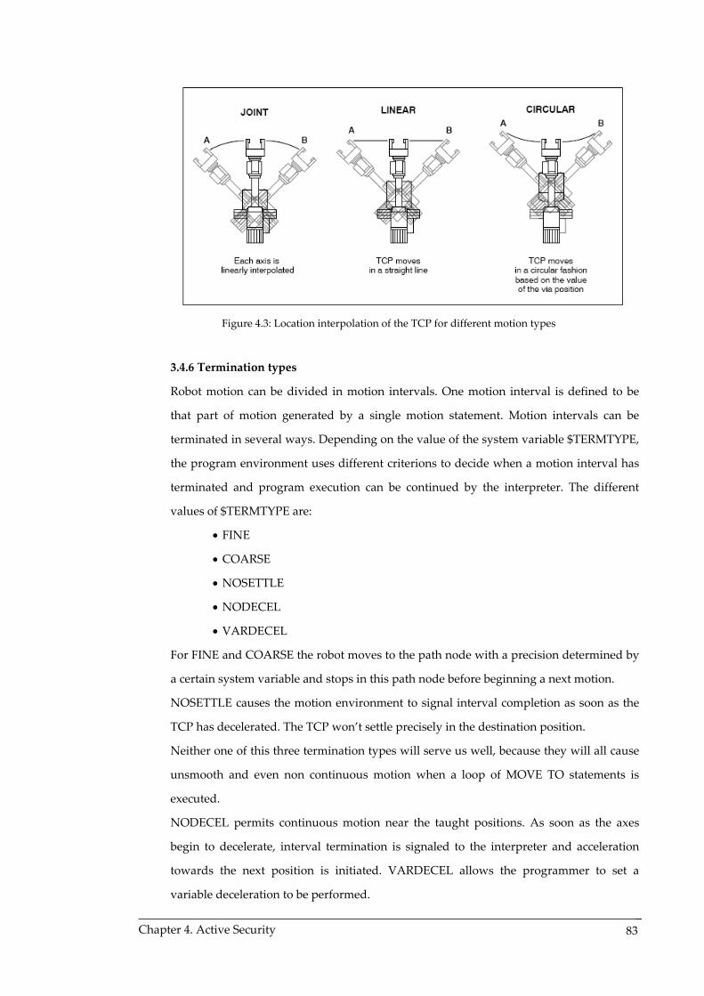
Figure 4.3: Location interpolation of the TCP for different motion types

3.4.6 Termination types

Robot motion can be divided in motion intervals. One motion interval is defined to be

that part of motion generated by a single motion statement. Motion intervals can be

terminated in several ways. Depending on the value of the system variable $TERMTYPE,

the program environment uses different criterions to decide when a motion interval has

terminated and program execution can be continued by the interpreter. The different

values of $TERMTYPE are:

• FINE

• COARSE

• NOSETTLE

• NODECEL

• VARDECEL

For FINE and COARSE the robot moves to the path node with a precision determined by

a certain system variable and stops in this path node before beginning a next motion.

NOSETTLE causes the motion environment to signal interval completion as soon as the

TCP has decelerated. The TCP won’t settle precisely in the destination position.

Neither one of this three termination types will serve us well, because they will all cause

unsmooth and even non continuous motion when a loop of MOVE TO statements is

executed.

NODECEL permits continuous motion near the taught positions. As soon as the axes

begin to decelerate, interval termination is signaled to the interpreter and acceleration

towards the next position is initiated. VARDECEL allows the programmer to set a

variable deceleration to be performed. _Chapter 4. Active Security

83

Finally, we would like to mention the abnormal interval termination statements

CANCEL and STOP. These built‐ins can be used in global or local condition handlers.

When a CANCEL statement is invoked in a condition handler, the motion interval is

considered completed immediately. The motion environment signals the interpreter and

the MOVE statement is terminated. The robot’s axes are decelerated to a halt.

A STOP causes the motion of the axes to stop. However, it does not cause interval

termination. The robot stops moving, but the unexecuted motion is put on a stopped

motion stack and the motion can be resumed. The interval will not terminate until the

motion has been resumed or terminated normally. If no NOWAIT clause (see further on)

is used, program execution is thus halted, because the interpreter is waiting for the

motion interval to complete.

In our active security application, upon detecting of an obstacle, normal trajectory

execution needs to aborted immediately. We therefore use a CANCEL statement in a

global condition handler. We refer to Appendix C for programming details.

3.4.7 Motion clauses

Optional clauses included in a MOVE statement can specify motion characteristics for a

single move or conditions to be monitored during a move (i.e. a local condition handler).

Clauses that have proven to be very useful in our application are the WITH clause and

the NOWAIT clause.

The WITH clause allows you to specify a temporary value for a system variable, e.g. a

motion or termination type. The motion environment uses this value while executing this

MOVE only. At termination of the MOVE, the temporary value ceases to exist.

The NOWAIT clause allows the KAREL interpreter to continue program execution

beyond the current MOVE statement while the motion environment carries out the

motion.

If used in combination with the termination type NODECEL, the NOWAIT clause has

proven to realize a satisfying continuous motion if consecutive MOVE TO statements are

executed on a series of XYZWPR variables that are not gathered in a PATH variable. This

guaranteed us that continuous motion along the alternative positions could be started up

before knowing all of these alternative positions. For, implementing MOVE TO

statements with NOWAIT clauses in a loop results in a motion in which no deceleration

nor discontinuity are noticed.


84

Figure 4.2 depicts the effect of $TERMTYPE and the NOWAIT clause on motion

execution.

Figure 4.2: Effect of $TERMTYPE on path motion

As can be seen from figure 4.2, we have to bear in mind that combining the NODECEL

termination type with NOWAIT clauses causes the TCP not to pass through the exact

destination location. In practice, this effect has proven to be very small for low motion

speeds.

To terminate the paragraph on motion control, we state a KAREL program line of a

MOVE ABOUT statement with a $TERMTYPE and NOWAIT clause:

WITH $TERMTYPE = NOSETTLE MOVE ABOUT x_axis BY alpha

The variables x_axis and alpha have to be previously declared and initialized as

VECTOR and REAL data types respectively.

We would like to point out that we only highlighted some of the numerous aspects on

KAREL motion. For more information, e.g. on acceleration and deceleration mechanisms,

system variables related to speed, acceleration and deceleration, controller interpolation

methods,…, we refer to the KAREL Reference Manual [15].


85

3.5 Read and write operations

A KAREL program can perform serial I/O operations on data files residing in the KAREL

file system and on serial communication ports associated to connectors on the KAREL

controller.

In paragraph 4 on real‐time communication we will elaborate how information can be send

from inside a MATLAB session to a running KAREL program over Ethernet. This will be

possible because the KAREL system provides us with the necessary tools to activate

Ethernet sockets and perform file input and output operations through these sockets.

Sockets can be seen as Ethernet activated communication ports that enable data exchange

between an external device and the robot controller. Details on this communication will be

given in paragraph 4.

Fundamental mechanisms in the established socket communication are file input and

output operations. Data files or communication ports can be opened, read from or written

to and closed. We will now highlight the elements that are involved in this process: file

variables, file operations and the input/output buffer.

3.5.1 File variables

A FILE variable is used to indicate the file or communication port on which you want to

perform serial I/O operations. A FILE is declared in the VAR section of the program end

initiated by associating it to a specific file or communication port in the OPEN FILE

statement. The CLOSE FILE statement disconnects the FILE and makes it possible to use

the variable to read or write from another file or communication port.

3.5.2 File operations

Besides the OPEN FILE and CLOSE FILE operations, two basic file operations are

available: READ and WRITE. The data items that have to be read or written, are stated as

parameters of the specific function.

More built‐ins are provided by the KAREL system. E.g., file attributes can be set using

the SET_FILE_ATTR built‐in.

For details about file operation built‐ins, we refer to the KAREL Reference Manual [15].


86

3.5.3 Input/output buffer

An area in RAM, called a buffer, is used to hold up to 256 bytes of data that has not yet

been transmitted during a READ or WRITE operation. Especially for the on‐line data

exchange between a pc and the controller, this buffer will be of importance. The moment

data is sent over a socket and received by the controller, this data is temporary stored in

the buffer before a READ operation is performed on the FILE associated to the socket. To

check if data has already been received from a serial port, the KAREL built‐in

BYTES_AHEAD is of indispensable importance. BYTES_AHEAD checks to state of the

buffer associated to a specific FILE and returns the number of buffered bytes that are

ready to be read in.

3.5.4 Example: reading in an array of XYZWPR variables

For our application, reading in positional variables is of high importance. Alternative

positions are calculated for in MATLAB and subsequently need to be transmitted to the

controller, read in and stored in KAREL positional variables. With the following example,

we want to illustrate how an ARRAY OF XYZWPR pos_array is read in from a FILE

called data_file. Hereby, it is important to know that arrays need to be read in element by

element in a for‐loop and that for XYZWPR variables, every field needs to be read in as a

separate REAL variable. The extension .dt is the typical KAREL format specifier for data

files that are stored in the KAREL system. The file data.dt contains num_nodes rows of 6

REAL variables that are separated by a backspace delimiter.

OPEN FILE data_file(‘RW’, ‘data.dt’) FOR i=1 to num_nodes DO

READ data_file(pos_array[i].x) READ data_file(pos_array[i].y) READ data_file(pos_array[i].z) READ data_file(pos_array[i].w) READ data_file(pos_array[i].p) READ data_file(pos_array[i].r)

ENDFOR CLOSE FILE data_file

3.6 Multi‐tasking

Multi‐tasking allows more than one program to run on the controller on a time‐sharing

basis, so that multiple programs appear to run simultaneously. For our active security

application, we will design a set of processes of which each one has its specific


87

functionality in the overall system. The multi‐tasking mechanisms of the KAREL system

will be used to introduce a certain interaction between these processes.

A term commonly used in multi‐tasking is a task. A task is a user program that is running

or paused. A task is executed by an interpreter. Interpreters are system components to

which a task is assigned when it is started. The system interpreters are capable of

concurrently executing tasks.

3.6.1 Task scheduling

It is important to be aware that although multiple tasks seem to operate at the same time,

they are sharing use of the same processor. At any instant only one task is really being

executed.

Once execution of a statement is started, it must complete before statements from another

task can be executed. The only exceptions on this rule are formed by the interruptible

statements: MOVE, READ, DELAY, WAIT and WAIT FOR. While waiting for a motion

or read operation to complete, a task is in a hold condition. The DELAY, WAIT and

WAIT FOR statements are also hold conditions.

A task that is currently running will execute statements until one of the following events

occurs:

• A hold condition occurs;

• A higher priority program becomes ready to run;

• The task time slice expires;

• The program aborts or pauses.

A task is ready to run when it is in the running state and has no hold conditions. Only

one task is actually executed at a time. Task priority and time‐slicing will determine

which task will be executed when more than one task is ready to run.

3.6.1.1 Priority scheduling

If two or more tasks with different priorities are ready to run, the task with the highest

priority will run first. In KAREL, a default priority of 50 is assigned to each user task, ‐8

is the highest priority, 143 the lowest.

A task’s priority can be declared upon translation by using the %PRIORITY translator

directive after the first line in the .kl code. With the SET_TSK_ATTR built‐in the current

priority of a task can be set and thus changed wherever that is needed in the program

execution.


88

3.6.1.2 Time slicing

If two or more tasks of the same priority are ready to run, they will share the system

resources by time‐slicing, which is a mechanism of alternating use of the system. A

time‐slice permits other tasks of the same priority to execute, but not lower priority

tasks. For more details on priority scheduling and time slicing we refer to the KAREL

Reference Manual [15].

3.6.2 Parent and child tasks

Execution of a task can be invoked by another, already running task. The invoking

program is called the parent task and creates a new task, the so called child task. In

KAREL programs new tasks are created using the RUN_TASK built‐in. Once created, a

child task runs independently of the parent task.

A child task can use variables declared in the parent task if this variable is declared in the

child task with the same variable name and using the FROM clause. A BOOLEAN named

detection that is also declared in a parent task parent.kl, is declared in a child task of

parent.kl as follows:

VAR

detection FROM parent: BOOLEAN

Besides the RUN_TASK built‐in, there are a number of built‐ins used to control and

monitor other tasks in KAREL: PAUSE_TASK (to pause a task), CONT_TASK (to resume

a paused task), ABORT_TASK (to abort a task) and GET_TSK_INFO (to obtain the

current task state).

As task related condition handler actions we mention the PAUSE, CONTINUE and

ABORT built‐ins to respectively pause, resume and abort the task in which the condition

handler is defined and enabled.

3.6.3 Semaphores As previously seen, the KAREL controller allows us to create program structures that are

task oriented. A child task can be invoked from a parent task, in a specific moment of

program execution. This allows us to attribute the execution of sub processes to tasks,

that are programmed in separate .kl files. This way, a clear programming structure of the

parent task can be maintained and the functionality of the application can be amplified.


89

Previously we have seen, as possibilities to pass on program execution control from one

task to another, the priority assignment translator directive and the built‐in functions for

creating, pausing and resuming child tasks.

In nearly all program applications –and not only in the field of robot programming– that

incorporate the passing on of execution control between processes, semaphores have

proven to be of indispensable importance. Ever since Dijkstra introduced the use of

semaphores in 1968, semaphores have been widely recognized and implemented in

software systems.

The KAREL controller supports the use of counting semaphores and disposes of a set of

built‐in functions to perform operations on semaphores. For the design of our active

security system, we thankfully used semaphores to pass on program control between

tasks or routines in specific moments, e.g. when a condition handler is triggered.

The basic principles of semaphores and the possible operations and semaphores will now

be highlighted, as well as the KAREL built‐in instructions that correspond to the

semaphore operations.

3.6.3.1 Basic principles of semaphores

Semaphores are special integer variables in the universe where processes are declared

and running. Before parallel running processes are started up, semaphores are

initialized at a specific value, often being 0 or 1, depending on their application. After it

has been initialized, the value or count of a semaphore can be changed by using two so

called initialization primitives: the “wait” and “signal” operation.

3.6.3.1.1 Wait operation

When a process , i.e. a KAREL program, task or routine, executes a wait operation

on a semaphore, the semaphore count is decremented by 1. The resulting

semaphore count is then evaluated on being non‐negative (≥0) or negative (<0). If

the count is non‐negative, the process that executed the wait operation can

continue its normal execution. If the count is negative, the process is paused and

put in a buffer that is associated to the same semaphore.

3.6.3.1.2 Signal operation

A process that executes a signal operation on a semaphore causes the count of this

semaphore to be incremented by 1. If the resulting count is positive (>0), then the


90

signal operation doesn’t have any effect. If the resulting semaphore count is non‐

positive (≤0), one of the processes that was previously put on the buffer of the

semaphore is released and becomes ready to run again. If the task that executed the

signal operation maintains executing depends on its priority relation to the

released task.

Tasks are released from the buffer on a first in/first out basis. Every semaphore has its

own buffer.

It is important to state that semaphores need to be declared as a global variable in the

program tasks that use it. This way, the semaphore’s count is visible and accessible for all

tasks using it. In KAREL, a semaphore declared as an INTEGER in a parent task

PARENT.KL, needs to be declared in the parent’s child tasks CHILD_A.KL and

CHILD_B.KL with a FROM PARENT clause to make sure the child tasks can access the

semaphore. See Appendix C for a programming example.

Semaphores are software mechanisms. For the user, only the initialization, wait and

signal operations are visible and executable. However, in the kernel of the system the

primitive operations are backed up by a computer algorithm that implements the

semaphore mechanism described above.

In robot programming applications, semaphores are used to assure the mutual exclusion

of program tasks. This means that two or more tasks are programmed in such a way that

only one of the set can be active at the same moment. Mutual exclusion semaphores are

initialized at 1 and the first line of each program is a wait operation on the semaphore.

The first task that is executed decrements the semaphore count to 0 and can thus

continue its execution. When another task is run, it decrements the count to ‐1 and the

task is put on the semaphore’s buffer. When a signal operation is executed on the

semaphore, e.g. by the first program upon its termination, or within a condition handler,

the buffered task is released and run.

In table 4.1 the semaphore related KAREL built‐ins and description of their use are stated.

For the input parameters of each built‐in, we refer to KAREL Reference Manual [15]. It is

important to mention that only SIGNAL SEMAPHORE can be used as an action within a

condition handler.


91

KAREL built‐in Description

SIGNAL SEMAPHORE Signals the specified semaphore

CLEAR_SEMA Resets the semaphore count to 0

POST_SEMA Adds 1 to the semaphore count

PEND_SEMA Subtracts 1 from the semaphore count

SEMA_COUNT Returns semaphore’s current value

Table 4.1: Semaphore related KAREL built‐ins

3.6.4 Motion control

An important restriction in multi‐tasking lies in the control of the various motion groups.

Only one task can have control or use of a group of axes. A task requires the use of the

motion group if at least one MOVE statement is executed in the program.

The first task that is run and that contains MOVE statements, gets control of the motion

group. If a second motion executing task is attempted to be run, this results in an error,

for the task attempts to get control of a motion group that has already been assigned to

the first task.

This can be avoided by imposing that the task doesn’t ask control of the motion group

upon activation. This is realized by using the translator directive %NOLOCKGROUP.

When the task needs motion control at a certain point during its execution, the

LOCK_GROUP built‐in can be used to assign the motion group to the task. Two tasks

competing for control of a motion group can be provided with a semaphore based

mutual exclusion mechanism so that no task can execute a LOCK_GROUP statement

when the other task locked the group and hasn’t released it yet with an

UNLOCK_GROUP statement. For an example of this strategy, see the KAREL Reference

Manual[15].

Another solution is to execute all motion in the same task, but implement the alternative

motion in an interrupt routine of the task. For our active security application, we chose

this solution.

4. Real‐time communication

As seen in the introduction chapter of this thesis, in a real‐time communication system

information needs to be transferred at a rate that is sufficiently high for the given environment.

As important as the fastness of transfer is the guarantee that data transfer will complete within


92

a determined time. If transmission time is guaranteed, we call the communication system

deterministic.

In industrial settings, the traditional communication systems are fieldbus networks. A

commonly used field bus is the Pofibus (Process Field Bus) that allows transmission speeds up

to 500Kbit/sec. For Profibus, the real‐time condition is met because bus admission is controlled

by a token passing mechanism. A device can only start broadcasting when it is in possession of

a ‘token’. Sending devices (masters) pass the token on to each other and it is guaranteed that a

master will become in possession of the token within a certain time. Deterministic

communication is guaranteed for the Profibus types DP (Decentral Periphery) and PA (Process

Automation). For more details on field buses, we refer to literature [21].

Nowadays, the demand for Ethernet as a real‐time control network is increasing. As some of

the reasons we can mention the lower product costs in comparison to field buses, the

possibility to monitor data transmissions or the easy connectivity of office pc’s in order to

perform control operations on the industrial equipments. However, we cannot accept Ethernet

as a real‐time communication medium without making some important considerations.

Ethernet, as defined in IEEE 802.3, is unsuitable for strict real‐time industrial applications

because its communication is non‐deterministic. This is due to the definition of the network’s

media access control protocol that is based on Carrier Sense Multiple Access with Collision

Detection (CSMA/CD). For a thorough explanation of CSMA/CD mechanisms we refer to

literature on Ethernet. What it boils down to is that nodes connected to a same network can

start transmitting data packages at the same moment. When this happens, a collision of the

data packages occurs and information is destroyed. The involved network nodes stop

transmitting and wait a random time that is determined by an exponential back‐off algorithm.

When their waiting time has past, each one of the involved nodes tries to transmit again. A new

collision is most unlikely, but can never be fully excluded. Networks nodes that can cause

collisions of data packages when they transmit, are said to be in the same collision domain.

In modern motion control applications such as robotics cycle times are typically hundreds of

microseconds ([16]). Traditional Ethernet and field bus systems are not capable of meeting

these high cycle time requirements.

Despite of all this, high‐speed Ethernet switches, full duplex Fast Ethernet (100Mbps) and

Gigabit Ethernet (1Gbps) have made it possible to use TCP/IP Ethernet connections to transmit

control signals and data.


93

4.1 Full duplex Ethernet

Modern Ethernet is designed as full‐duplex. This means that a network device can

simultaneously send and receive data. The Ethernet card installed in the device can begin

sending data while the process of receiving data is still going on, or the other way around,

it can begin receiving while sending of data is still going on.

4.2 Fast Ethernet switches

A switch is a specialized junction box that has multiple built‐in Ethernet ports and its own

processor. Only one device is connected to each port of the Ethernet switch. This causes

every connected device to be isolated onto its own collision domain. The chance for

collisions to occur is hereby totally eliminated. Since it are the collisions that determine the

non‐deterministic character of Ethernet, the use of an Ethernet switch can adjust an

Ethernet Local Area Network (LAN) to be deterministic.

Typically for industrial applications, key control equipment is isolated into collision

domains with a switch. For our application, five devices are connected to the switch: the

three Axis network cameras, the robot controller and the pc from which control actions are

monitored. This idea is presented in figure 4.5.

Axis205 GICcam 1

193.144.187.122

SWITCHFANUC Arc Mate 100iB

193.144.187.156

PC

193.144.187.250

Axis205 GICcam 2

193.144.187.123

Axis205 GICcam 3

193.144.187.17

Figure 4.5: TEISA Local Area Network with Ethernet switch

Unlike a classical repeating hub that passes on sent data frames from the sending device to

all devices connected in the LAN, a switch can be trained to send data only to the

destination device. Data frames received by the switch are initially forwarded to each of the

switchʹs ports, but as the switch learns which MAC address is associated with which port,


94

it forwards data frames only to the port associated with the frameʹs destination address.

_

SA lab establishes a Fast Ethernet

sing the OSI Reference Model as the international standard for protocol layers in

n oriented protocol is TCP, which stands for Transmission

ient needs to

ge of data, such as

This allows several systems to simultaneously communicate full duplex and at full speed,

for a switch offers the full bandwidth to every connected device, where a repeating hub

divides the bandwidth between all connected devices.

The high‐speed Ethernet switch installed in the TEI

(100Mbps) connection between the connected devices of figure 4.5.

U

communication systems, we can situate Ethernet in the Data Link layer of OSI, for Ethernet

provides functional and procedural means to transfer data between connected network

entities. On top of the Ethernet protocol other protocols are used to exchange data packages

between connected devices.

A commonly used connectio

Control Protocol. TCP works in the Transport layer of the OSI model. Using TCP, data can

be sent in a stream with the guarantee that data will arrive in the order it was sent. If

communication errors occur, as well in the data itself as in the data order, this can be

corrected because of the way the protocol is implemented. TCP packages need to be formed

according to strict rules on the format of package headers. Headers are bit packages with

specific functions. Among others we can mention the communication port number of

sender and receiver, the header length, the acknowledge receipt flag and the checksum. For

more details, we refer to section 4.3.3 of this chapter and to literature on TCP.

TCP connections are initiated following a specific connection procedure. A cl

send a request for connection to a server that accepts the connection with the client by

returning an acknowledgement package. Subsequently, the client answers the server with

an acknowledgement for connection acceptance. From then on, client and server are

connected and synchronized and can start exchanging data packages.

Due to the extensive and time consuming activities in the exchan

checking if data is received in the correct order, sending of acknowledgements, retries in

transmission if errors occurred,…, the TCP protocol isn’t very suitable for real‐time

communication where data needs to arrive with a 100% guarantee and within a determined

time interval. However, combined with Fast Ethernet and switches, TCP has proven to be

suitable for industrial real‐time communications. For robotics applications, FANUC Robotics

provides TCP communication options, such as Socket Messaging and the File Transfer

Protocol. We will now introduce the principles of TCP data exchanges through socket

connections between two network devices. After having elaborated the principles of socket


95

messaging, we will explain how the socket messaging option is used in KAREL programs

to set up a communication with a MATLAB session.

_

.3 Socket messaging

ware endpoint that establishes bidirectional communication between a server

A by its IP

e reserved ports. They are used for well

ation sequence to set up and use a socket connection is

4

What is a socket?

A socket is a soft

program and one or more client programs. The socket associates the server program with a specific

hardware port on the machine where it runs so any client program anywhere in the network with

a socket associated with that same port can communicate with the server program [17].

s this definition says, a socket is the identification of a machine, identified

address, with a corresponding hardware port. To set up the connection between a server

and a client through a socket, the IP address of the server needs to be specified together

with the physical communication port, that must be the same on client and server device.

Once the connection between two entities is established, both of them can communicate

according to a certain protocol, such as TCP. When a socket is created, a 32 bit number is

generated to identify the socket. A receiving socket is typically identified as an even

number and a sending socket as an odd number.

The communication ports between 0 and 1023 ar

known server applications (e.g.: 80 for http, 20 and 21 for ftp, 23 for telnet). The port range

between 1024 and 49151 can be used for user defined server applications. Typically, a port

between 1024 and 5000 is used.

The connection and communic

illustrated in the example of figure 4.6. A server is put in the listen state. When the client

requests a connection, the server accepts connection. Once connected, both client and

server can send and receive data. Either the server or the client can close the connection.


96

SERVER = Fanuc 193.144.187.156 – port 2007 Waiting for communication

CLIENT = pc port 2007

Initiating communication

TCP on top of ETHERNET Socket communication service

1. listen 2b. connect 5. close

2a. connect 5. close

3a. send 4b. receive

3b. receive 4a. send

Figure 4.6: Socket connection and communication sequence

Software to set up a socket communication can be developed in C, C++, Java, Perl or other

languages. For details on these software applications we refer to literature. In the following

sections, we will see how we can use preprogrammed socket functions to set up a

connection, to send and receive data and to disconnect the socket.

4.3.1 KAREL socket messaging option

The KAREL system fully supports the above described communication mechanisms. In

order to use the User Socket Mesg option R636 of the FANUC Handling Tool System

Software in KAREL programs, client or server ‘tags’ first need to be set up in the system.

A tag is a label to which the parameters needed to set up a socket communication are

assigned. If it concerns a client tag, the remote server’s IP address and the physical

communication port need to be configured. For a server tag, only the communication

port needs to be set.

Since the KAREL system provides methods to instantly detect when the server accepts a

client’s connection request, we designed the robot controller to be the server. This means

we have to set up a server tag ‘S1’. Using the teach pendant, this is done following the

key sequence MENUS—SETUP—HOSTCOMM—F4[SHOW]—SERVERS. After having

set up the server tag S1, the system variable $HOSTS_CFG[1].$SERVER_PORT needs to

be given the value of the chosen communication port, e.g. 2007 for a user defined server

application. The server tag is now ready for use in a KAREL program. For more info on

this procedure we refer to the FANUC Robotics SYSTEM R‐J3iC Controller Internet

Options Setup and Operations Manual [18].


97

Three socket message related built‐ins are provided by the KAREL system: MSG_DISCO,

MSG_CONNECT and MSG_PING. They are used to respectively disconnect, connect and

‘ping’ a client or server socket. For more details we refer to the KAREL Reference Manual

[15]. The use of a socket in a KAREL program is illustrated by the following .kl source

code:

PROGRAM socket

VAR

ComFile: FILE

Status: INTEGER

BEGIN

MSG_DISCO(‘S1:’, Status) ‐‐ closing communication port before start

MSG_CONNECT(‘S1:’, Status) ‐‐ open port for communication

WAIT FOR Status = 0 ‐‐ wait until client device connects

OPEN_FILE ComFile(‘RW’, ‘S1:’) ‐‐ open FILE variable associated to socket

… [read and write operations on ComFile]

CLOSE_FILE ComFile ‐‐ close FILE variable

MSG_DISCO(‘S1:’, Status) ‐‐ disconnect server socket

END socket

If waiting for data to arrive through the communication port, a useful KAREL built‐in is

BYTES_AHEAD. With this function, we can detect if new data is received over an

opened communication file and is ready to be read in by the system. This method will be

used to watch if the obstacle detection signal has been sent from the pc.

For the programming applications of KAREL sockets, we refer to the program comm.kl

in Appendix C.

4.3.2 Socket messaging and MATLAB

Since all positional calculations and vision related operations are performed in MATLAB,

it is desirable that we are able to exchange data information between MATLAB and the

robot controller in an elegant and time efficient way. The KAREL controller offers us the

option of socket messaging from the robot’s side. On the support website of MATLAB we

found a toolbox that is designed to set up a socket communication between MATLAB

sessions of two network connected pc’s. The toolbox MSocket is designed by Steven


98

Michael of the MIT Lincoln Laboratory. The package contains a series of functions

written in C++ and compiled to MATLAB executable .dll function files. The toolbox offers

the following functions:

• mslisten: makes the server listen to connection requests by a client on a specific

port;

• msconnect: a client requests connection to the server, specifying the server’s IP

address and communication port;

• msaccept: the server accepts connection to the client;

• mssend: to send a single variable over the socket;

• msclose: closes the socket connection.

Compatibility of KAREL and MATLAB functions for creating socket connections and

sending variables had to be tested. It was found that string variables can be successfully

sent from MATLAB over the socket to a receiving KAREL program. In the next paragraph

we will comment some more details about the format of the sent data packages and some

specific communication issues.

Thanks to the socket toolbox of Steven Michael it was made possible to directly send data

from a MATLAB session to a KAREL program in an elegant and time efficient way.

For our active security application, the actual position of the Tool Center Point needs to

be sent from the KAREL system to MATLAB, because the fuzzy system needs this position

as a start point for the calculation of alternative path positions. The socket package for

MATLAB however doesn’t support a communication in this direction. We therefore used a

simple client socket application written in Perl, that is based on the good Perl program

examples that can be found in the Perl Black Book[19], written by Steven Holzner. The

code of the program Client.pl is added to Appendix C. The program establishes a socket

connection with a server that is waiting for a client to connect at a specific

communication port. Upon connection and creation of the socket, the client receives all

information that is sent by the server, as long as the socket is not disconnected. Perl

scripts can be called in MATLAB and we successfully tested this to receive the actual Tool

Center Point’s position from the KAREL system.

4.3.3 Format of data packages

TCP data packages consist of a header section and a data section. The package header

contains all information that is needed to successfully perform all steps in the


99

transmission protocol. Figure 4.7 illustrates the structure of a TCP package. Without

wanting to give a thorough explanation on the function of each field in the TCP package,

we can mention the source and destination port of the data package, the sequence

number, the acknowledgment number and the checksum. A sequence number is

assigned to each package to make sure no packages are lost and that the data is delivered

in the right order. The acknowledgment number is used in the procedure that confirms if

packages have been successfully received. The checksum allows the Transmission

Control Protocol to check if no bytes have been corrupted. For the functions of the other

fields, we refer to literature on the Transmission Control Protocol.

Bytes Field Description

0 ‐ 4 Source Port Destination Port 5 ‐ 8 Sequence Number 9 ‐ 12 Acknowledgment Number 13 ‐ 16 Data Offset Reserved Flags Window 17 ‐ 20 Checksum Urgent Pointer 21 ‐ 24 Options 24+ Data

Figure 4.7: Header fields of a TCP data package

When a data package is sent from MATLAB to a receiving KAREL program, incoming

bytes are stored in the KAREL system buffer that can contain up to 256 bytes. In the

KAREL program comm.kl of Appendix C, it is illustrated how incoming bytes can be

stored one by one in an ARRAY OF STRING variables. When testing the set up

communication between MATLAB and KAREL, it was found that some of the first 24

elements of the ARRAY variable contained meaningless information, originating from

the information in the packages headers. After reading in a new data package in KAREL,

the first 24 characters of the read in ARRAY OF STRING need to be discarded. For us,

useful information starts at position 25 in the ARRAY. For the application written in Perl,

no characters corresponding to the package headers were found after receiving the data

in MATLAB. Depending on the different software languages used for the socket

applications and the compatibility between these applications, we need to discard to

package header bytes manually or not.


100

4.3.4 KAREL communication program comm.kl

In section 5 of this chapter a solution to the active security problem will be proposed. In

this solution, a robot application written in KAREL will be introduced. The key program

of the application is a task in which all communicational interactions between the

KAREL system and our pc are situated. The three main communication tasks of the

KAREL program comm.kl (see Appendix C) can be described as follows:

• Receiving an obstacle detection signal through a socket connection;

• Sending back the actual Tool Center Point’s position through a socket;

• Receiving alternative positional and rotational data, sent in packages over

the socket.

As stated earlier, we have chosen the FANUC robot to act as the server in all

communication processes. The reason is that the KAREL system allows us to set a WAIT

FOR action after a MSG_CONNECT is called to connect a server tag. Only when a client

is effectively connected to the specified port of the server in the listen state, the WAIT

FOR statement is triggered and program execution continued.

For the receiving communication actions, one KAREL server tag ‘S4’ is used. At the

beginning of program execution, a MSG_CONN action is performed to put the server in

the listen state. As soon as a MATLAB socket is created and connected to the FANUC robot,

the program comm.kl starts checking if new data has entered the system’s input buffer.

For the sending communication action, we designed the Perl script Client.pl. Because a

new socket is created for this application, we had to set up another KAREL server tag ‘S3’

that listens for connections to another physical port of the FANUC device. Server tag ‘S4’

listen for connections to port 2007, while ‘S3’ listens for connections to port 2008.

For more details about the three communication steps, we refer to Appendix C. To

understand the program code, we would like to highlight the strategy used to read in the

alternative positional data.

As explained in paragraph 2.9.3 of chapter 3, we send data packages from MATLAB that

contain four alternative positions and rotational configurations. In order to be read in

successfully by the KAREL system, these numeric data has to be converted to the string

format. This operation can be symbolically written as in expression (4.2). The conversion

int2string consists in the transformation of positions x, y and z (expressed in integer

millimeters) and angles α and β (values in degrees of either ‐90, 0 or +90) to a string in

which s indicates the sign of each numeric value. If the numeric value is smaller than


101

1000, extra ‘0’ strings need to be padded to obtain a field of five characters for each

numeric position value and three characters for every angle.

[x, y, z, α, β] ’sxxxx syyyy szzzz sαα sββ’ (4.2) ⎯⎯⎯ →⎯ stringnti 2

In fuzzy_comm.m of Appendix B these strings are created after the calculation of every

fourth alternative position. Four of these positional strings are concatenated and sent to

the robot controller. Because every alternative position and angular configuration is

created in a uniform way, the KAREL program comm.kl is capable to extract all

information and convert the STRING variables to the INTEGER data type.

When the last alternative path node is calculated in MATLAB, a special string value ‘S’ is

padded to the last data package to indicate the termination of the alternative path. The

KAREL system is programmed so that this ‘S’ is detected and all read operations are

stopped. For program implementation details, we refer to comm.kl in Appendix C.

4.4 Real‐time performance of the Ethernet communication

When testing the communication system, very satisfying results were obtained. Times to

execute socket communication actions were measured using the available timing variables

of MATLAB (tic & toc, clock, etime) and the KAREL system (CONNECT TIMER and

DISCONNECT TIMER built‐ins).

The upper time limits of some actions are stated in tables 4.2 and 4.3. Especially the

execution time of the Perl script Client.pl gives us a good idea about the time needed to

perform communicational actions. Client.pl establishes a connection to the server tag ‘S3’

listening at port 2008, receives the actual Tool Center Point position and is ended upon

closing of the server tag ‘S3’ in the KAREL program comm.kl. It therefore incorporates

connection time, sending time and disconnection time. In table 4.3, tcp_x is an integer

variable containing the x position of the Tool Center Point. The zero times indicated with a

(*) need to be interpreted as times smaller then the counting step of the timer feature. In the

KAREL system, the result of the TIMER operations is determined by the system variable

$SCR.$COND_TIME that indicates the step with which the TIMER is incremented. For our

robot this system variable has a minimum value of 4 milliseconds. The execution times of

the statements MSG_DISCO, MSG_CONNECT and WRITE are therefore smaller than 4

milliseconds, but not equal to 0.


102

MATLAB socket action Upper time limit [msec]

msconnect 0 (*)

mssend 0 (*)

perl(‘Client.pl’) 160

msclose 0 (*)

Table 4.2: Socket communication times for MATLAB actions

KAREL socket action Upper time limit [msec]

MSG_DISCO(‘S3’, Status) 0 (*)

MSG_CONNECT(‘S3’, Status) 0 (*)

WRITE ComFile(tcp_x) 0 (*)

READ 110 bytes in input buffer 240

Table 4.3: Socket communication times for KAREL actions

5. The active security problem

Having solved the socket communication issue and knowing the possibilities of the KAREL

programming language, we now have all tools available that are needed to solve the active

security problem in a KAREL application.

A robot active security system can be seen as a safety backup for the normal robot task. When

an unexpected event occurs, e.g. a foreign object enters the robot’s workspace, this has to be

signaled to the robot. Motion along the regular trajectory is then cancelled, and thanks to an

input stream of information, motion along an alternative path is started up to guarantee the

robot will reach its original destination.

Tools such as condition handlers, semaphores, the system’s input buffer, routine structures,

priority scheduling and sharing variables among different KAREL programs are especially

created by FANUC to allow the implementation of complex user applications. Although a lot of

thinking work preceded the implementation of a solution to the active security problem, a

solution was relatively easy to create thanks to the mentioned programming features.

5.1 A solution in KAREL

We designed a solution to the active security problem in a task oriented way. A parent task

called secure.kl is created to run two child tasks and to initialize some important shared

variables used by both child tasks. One child task is in charge of executing all robot motion


103

and is called moves.kl. The other child task performs all communicational tasks and is

called comm.kl. We will first give a short description of each program.

5.1.1 Secure.kl

A count semaphore mutex for mutual exclusion is created in the VAR section and

initiated in a ROUTINE. As shared variables for the child tasks are created in the VAR

section:

• detect: an INTEGER data type that becomes 1 upon detection of the obstacle;

• halt: an INTEGER data type that indicates if reading operations have ended;

• count: an INTEGER data type that indicates the number of read in alternative

positions;

• xyz_data: an ARRAY[num_nodes, 5] OF INTEGER that will contain the

alternative path positions and rotational configurations.

The ARRAY OF INTEGER xyz_data will be filled up with data by comm.kl and used by

moves.kl to execute the alternative motion. The INTEGERs are initialized at 0 in a

ROUTINE of secure.kl. In the MAIN section of secure.kl, the ROUTINEs to initialize the

semaphore and the shared variables are called. Subsequently, the two child tasks are run.

Note that, once the two tasks are run with the RUN_TASK built‐in, the program secure.kl

ceases to exist, it is aborted. The child tasks now operate independent of their parent.

However, the .vr file of secure.kl stays accessible for use by moves.kl and comm.kl.

5.1.2 Moves.kl

The program moves.kl executes the normal motion trajectory in its MAIN section. Upon

triggering of a condition handler by the INTEGER detect becoming 1, this motion is

cancelled and an interrupt routine is invoked. In this interrupt routine, motion along the

alternative path is executed.

The shared variables detect, count, mutex and xyz_data are declared in the VAR section

with a FROM secure clause.

5.1.3 Comm.kl

As already introduced in section 4.3.4, comm.kl receives the detection signal from

MATLAB, sends the current Tool Center Point position back to MATLAB, receives the


104

positions and rotations along the alternative path and stores them in xyz_data. The same

shared variables are declared in the VAR section.

5.1.4 Task priorities

We chose to give the communication task comm.kl a higher priority then moves.kl. The

philosophy followed to make this decision is that important information entering the

KAREL system needs to have precedence to the execution of motion statements. For

example, it is not allowable that a ‘1’ for a detected signal has already entered the system,

but cannot be read out the buffer because moves.kl is evaluating a MOVE statement.

However, we mention that assigning a higher priority to moves.kl isn’t impossible either

because evaluating MOVE statements only consumes a few milliseconds of processing

time. MOVE statements are interruptible statements. This means that during the motion

of a MOVE, the program moves.kl is in a hold state, and comm.kl then gets full attention

of the Central Processing Unit.

However, we made the choice to assign the higher priority of 49 to comm.kl, while

moves.kl has the default priority of 50. Therefore comm.kl is constantly checking the

system input buffer, unless it is in a hold state. If comm.kl would never come in a hold

state, moves.kl would never get an opportunity to execute, for comm.kl has a higher

priority. To give moves.kl a chance to be executed, we included a DELAY of 20ms

between two BYTES_AHEAD operations that check if any bytes of the detect signal have

arrived in the input buffer. We realize that including a DELAY statement in a higher

priority task is a form of busy waiting. However, for the reason of absolute priority of

communication information, we implemented the priorities in this way.

The function and main properties of the tasks secure.kl, moves.kl and comm.kl are qualitatively

illustrated in figure 4.8.


105

VAR detect, mutex, halt, count: INTEGER xyz_data: ARRAY OF INTEGER

secure.kl

RUN_TASK(‘moves’) RUN_TASK(‘comm’)

%PRIORITY = 50

VAR detect, mutex, halt, count FROM secure:

INTEGER xyz_data FROM secure:

ARRAY OF INTEGER

%PRIORITY = 49

VAR detect, mutex, halt, count FROM secure:

INTEGER xyz_data FROM secure:

ARRAY OF INTEGER

moves.kl

comm.kl

Figure 4.8: Architecture of KAREL active security solution.

5.1.5 Semaphore use and program execution dynamics

In this section we want to comment the dynamical cooperation between the two tasks

comm.kl and moves.kl. To help understand the following explanation, the execution

dynamics of both tasks are schematically represented in figure 4.9. An axis indicates the

evolution of time during program execution. The condition next to each arrow triggers

the following step in program execution.

When both tasks are started up by secure.kl with the RUN_TASK statement, the first task

that receives execution time of the Central Processing Unit (CPU) is comm.kl, for it has a

higher priority. In the WHILE loop that checks if data has been received in the system’s

input buffer, a DELAY statement of 20ms is incorporated to give moves.kl execution time.

The robot starts moving between a Start and Final position (XYZWPR variables). DELAY

statements of 1000ms are introduced to simulate the time of a manipulation action in the

end points of the trajectory. This motional action is repeated as long as no detect = 1

signal has been read from the system’s input buffer. The BYTES_AHEAD operation on

the buffer is repeated as long as no bytes have arrived in the input buffer (BufBytes = 0).

When a detect = 1 signal is detected, comm.kl suspends itself by pending the semaphore

mutex with the PEND_SEMA built‐in. Subsequently, a global condition handler in

moves.kl is triggered. The normal motion loop is instantaneously cancelled and the


106

interrupt routine alternative for execution of the alternative path is invoked from the

condition handler. The first action of the routine alternative is signaling the semaphore

mutex that was earlier pended by comm.kl. Comm.kl takes over the CPU control. It uses

this control to put the server tag ‘S3’ in a listen state at port 2008. At this port, the FANUC

robot will receive a connect request by the Perl script Client.pl. As long as this Perl script

is not executed in MATLAB, the task comm.kl is in a hold state, for we implemented a

WAIT FOR statement that suspends program execution until the connection of the socket

has been successfully established. Moves.kl takes over CPU control when comm.kl is in

this hold state. However, moving along the alternative path isn’t possible, because no

alternative positions have been read in yet. Therefore, moves.kl suspends itself by

invoking a PEND_SEMA action on the semaphore mutex.

As soon as the Perl script is executed in MATLAB, a socket connection is established.

Comm.kl registers the current Tool Center Point position and sends it over the socket

port 2008 to MATLAB. There, the program fuzzy_comm.m is invoked using as arguments

the current Tool Center Point position and the obstacle position calculated with the

artificial vision system. As soon as the first data package is calculated, it is sent over the

socket connection to the FANUC server tag ‘S4’ at port 2007, earlier opened to receive the

detection signal. When the first positions are received by comm.kl, the semaphore mutex

is signaled by comm.kl. This way, execution of the interrupt routine in moves.kl is

resumed and motion along the alternative path is initiated. With a delay of 80ms, needed

to give moves.kl processing time, the next data packages sent from MATLAB are read in

by comm.kl. When the stop string ‘S’ is encountered in the data packages, it means that

all alternative positions were calculated and sent in MATLAB. The task comm.kl aborts,

for all executable statements in the MAIN section have been executed. When the final

destination of the alternative path is reached, moves.kl returns from the interrupt routine

alternative and is also aborted.

We would like to state that this solution is one that works, but that it surely isn’t the only

solution to the active security program. Experienced KAREL programmers might be able

to implement a solution that has a more solid structure and that consumes CPU time in a

more efficient way.


107

moves.kl comm.kl

MOVE TO Start DELAY 1000 MOVE TO Final DELAY 1000

WHILE detect = 0

CONDITION[1]: WHEN detect = 1

Execute alternative trajectory

ABORT

1. BYTES_AHEAD statement on system input buffer 2. DELAY 20

WHILE BufBytes = 0

IF detect = 1

1. CANCEL motion 2. Call interrupt routine Alternative 3. POST_SEMA

PEND_SEMA

WAIT FOR in comm.kl

PEND_SEMA

WAIT FOR connection to ‘S3’ on

port 2008

1. Socket connected at port 2008 2. Send actual TCP position 3. Receive first data package 4. POST_SEMA 5. Continue read operations

ABORT

String ‘S’ received

POST_SEMA by comm.kl

POST_SEMA by moves.kl

Final position reached

Call to Client.pl script in MATLAB

tfinal

t0

RUN_TASKRUN_TASK

Figure 4.9: Execution dynamics of moves.kl and comm.kl.


108

We end this paragraph on the KAREL solution of the active security problem with the

remark that the designed security system is not a cyclic one. Once an alternative path is

executed, all programs come to a natural end, they are aborted. In a more automated

design, it would be desirable that robot motion continues when the final position is

reached. A more thorough interaction between the KAREL communication task and the

vision system would be required to signal if the obstacle is still present in the work space

or not. If it is still present, a new alternative trajectory has to be followed. If it is not

present anymore, the robot can return to executing its normal activity. The programming

of such a KAREL application is however left for future investigators.

6. Experimental results

The presented KAREL solution for the active security problem was tested in an integrated way

with the fuzzy artificial intelligence system. Very fast reaction times to a sent obstacle detection

signal were observed. Subsequently, the current Tool Center Point is quasi instantaneously sent

over a socket. Alternative position and rotation packages were created in the string format

elaborated in section 4.3.4 and sent over a socket in the function fuzzy_comm.m of Appendix B.

Upon receiving the first data package (within 400 milliseconds), the motors of the robot’s axes

immediately start accelerating and motion is initiated. Even before motion has visually started,

all data packages have been received by the system.

In debugging and testing KAREL programs, KAREL statements to write messages to the screen

of the Teach Pendant have proven to be very useful to follow the program execution steps. We

refer to Appendix C for programming details. We also have to state that the home page of the

robot (http://robot or http://193.144.187.156 in the LAN of the TEISA research group) is a very

useful tool, especially to follow the current state of activated programs and to consult the

values of program data after program execution has terminated.

In a second phase, the artificial vision system was integrated in the overall system. Upon

detection of the obstacle, the obstacle detection signal is sent quickly over the socket and robot

motion is halted. Between the sending of the obstacle detection signal and asking for the Tool

Center Point’s current position, the vision system calculates the obstacle’s position. During this

time, the KAREL programs comm.kl and moves.kl are both in a suspended state, for comm.kl

is waiting for a connection to ‘S3’ at port 2008 and moves.kl is suspended by a PEND_SEMA

action. Since the calculation of the obstacle’s position in the work space is the most time

consuming process in the whole active security system (see table 2.4), the robot’s End Effector

is noticeably paused at this moment, up to a time of three seconds.


109

http://robot/

http://193.144.187.156/

In the programmed application, a translational motion speed of 200 mm/sec and rotational

speed of 90 °/sec were used.

A MATLAB script to execute the active security system with the vision and fuzzy systems

incorporated is added to Appendix C.

Readers that want to see the robot and the active security in action, can request a movie by

sending an e‐mail to the author of this thesis ([email protected]).

7. Acknowledgments

Special thanks goes to Hugo Herrero of FANUC España for his support in KAREL

programming issues and for proposing the socket messaging communication.

In a critical moment of this project, Dieter Debaillie of FANUC Belgium helped us out to

establish the User Socket Msg option in the robot’s system software. He also provided us with a

key KAREL example for socket communication.

Thanks goes to Antonio Jenaro for his knowledge transfer in Ethernet configurations of

network devices and for installing and configuring the Fast Ethernet switch in the TEISA

laboratory.

Finally, most special thanks goes to professor José Ramón Llata for his intensive support

during the last busy months of this project and for proposing the Perl socket communication,

hereby solving the last missing link.

8. References

[14] FANUC Robotics España, FANUC Robotics Curso de Progamación TPE, Nivel B.

[15] FANUC Robotics America, Inc., FANUC Robotics SYSTEM R‐J3iC Controller KAREL

Reference Manual, 2006.

[16] Real time Ethernet I, Introduction to Real‐Time Electronic Control Systems,

http://industrialethernetu.com/courses/

[17] http://java.sun.com/developer/onlineTraining/Programming/BasicJava2/socket for the

definition of an Ethernet socket.

[18] FANUC Robotics America, Inc., SYSTEM R‐J3iC Controller Internet Options Setup and

Operations Manual.

[19] Steven Holzner, Perl Black Book, The Coriolis Group, 1999.

[20] What makes Ethernet industrial?, www.neteon.net.

[21] L.J.M. Van Moergestel, Computersystemen en Embedded Systemen, 2e herziene druk,

Academic Service, Den Haag, 2007.


110

mailto:[email protected]

http://industrialethernetu.com/courses/

http://java.sun.com/developer/onlineTraining/Programming/BasicJava2/socket

http://www.neteon.net/

[22] www.wikipedia.com for information on Ethernet and the Transmission Control Protocol.


111

http://www.wikipedia.com/

Chapter 5 Conclusion In this Master’s Thesis, an active security system for an industrial FANUC robot was introduced.

The fundaments of the security system are formed by an artificial intelligence and an artificial

vision system.

Known stereo vision techniques were introduced to design a vision method that can identify

and localize obstacles of certain characteristics in the robot’s workspace. Given the vision tools

available in this project, a user friendly and time critical method was developed to check the

robot’s workspace for obstacles. The key element to this solution was the use of ActiveX

components that allow us to draw camera images out of a video stream of images.

If camera images need to be available at a higher time rate, cameras equipped with frame

grabbers can always be installed for future projects.

Basic methods for object recognition were employed. In future investigation work, advanced

identification methods can be used, e.g. to distinguish the robot’s End Effector from foreign

objects.

In the proposed real‐time setting, the time needed to calculate the characteristic positions of a

cubic obstacle was rather high, in some cases up to 2.5 seconds. A better technique can be

developed to calculate for obstacle corners.

The artificial intelligence technique Fuzzy Logic was successfully applied for the design of a 3D

obstacle avoidance strategy. Following all basic steps in the design of a Fuzzy Inference System,

this strategy was developed and simulated in MATLAB. Thanks to the designed communication

system, alternative path positions and rotational configurations could be transferred to the

robot’s system at a time critical rate.

Finally, using Ethernet as communication medium for the robot control, a real‐time solution to

the active security problem was developed in the programming language KAREL of FANUC

Robotics.

As this project has been the first one on the FANUC Robot Arc Mate 100iB of the research

group TEISA, a great deal of the investigation time was consumed in getting to know the

robot’s programming language KAREL and in setting up a communication system through

Ethernet sockets. However, we believe that the security application presented in the previous

chapter is a strong solution to the given problem and a very good example of the KAREL

system’s possibilities. Moreover, socket communication is an elegant and fast way to exchange

data between control pc’s and robot controllers. And, as Ethernet is working its way up to the

_Chapter 5. Conclusion

112

industrial work floor, the socket communication is a valid industrial solution today and will

probably maintain its strong position in the years to come.

As mentioned at the end of the previous chapter, a more automated KAREL application can be

designed in which robot motion continues when the final position of the alternative path is

reached. For this application, a more thorough interaction between the KAREL communication

task and the vision system would be required to signal the presence or the absence of an

obstacle in the robot’s work space. Subsequently, the decision to return to the normal robot task

or to follow a new alternative path has to be undertaken. The programming of such a cyclic

KAREL application is left as a challenge for future investigators.

_Chapter 5. Conclusion

113

Appendix A

function varargout = CamAxis(varargin) % CamAxis M-file for CamAxis.fig % CamAxis, by itself, creates a new CamAxis or raises the existing % singleton*. % % H = CamAxis returns the handle to a new CamAxis or the handle to % the existing singleton*. % % CamAxis('CALLBACK',hObject,eventData,handles,...) calls the local % function named CALLBACK in CamAxis.M with the given input arguments. % % CamAxis('Property','Value',...) creates a new CamAxis or raises the % existing singleton*. Starting from the left, property value pairs are % applied to the GUI before CamAxis_OpeningFunction gets called. An % unrecognized property name or invalid value makes property application % stop. All inputs are passed to CamAxis_OpeningFcn via varargin. % % *See GUI Options on GUIDE's Tools menu. Choose "GUI allows only one % instance to run (singleton)". % % See also: GUIDE, GUIDATA, GUIHANDLES % Edit the above text to modify the response to help CamAxis % Last Modified by GUIDE v2.5 22-May-2007 18:07:49 % Begin initialization code - DO NOT EDIT gui_Singleton = 1; gui_State = struct('gui_Name', mfilename, ... 'gui_Singleton', gui_Singleton, ... 'gui_OpeningFcn', @CamAxis_OpeningFcn, ... 'gui_OutputFcn', @CamAxis_OutputFcn, ... 'gui_LayoutFcn', [] , ... 'gui_Callback', []); if nargin && ischar(varargin{1}) gui_State.gui_Callback = str2func(varargin{1}); end if nargout [varargout{1:nargout}] = gui_mainfcn(gui_State, varargin{:}); else gui_mainfcn(gui_State, varargin{:}); end % End initialization code - DO NOT EDIT % --- Executes just before CamAxis is made visible. function CamAxis_OpeningFcn(hObject, eventdata, handles, varargin) % This function has no output args, see OutputFcn. % hObject handle to figure % eventdata reserved - to be defined in a future version of MATLAB % handles structure with handles and user data (see GUIDATA) % varargin command line arguments to CamAxis (see VARARGIN) % Choose default command line output for CamAxis handles.output = hObject; % Contador de paquetes de imágenes handles.cont=0; % Flags de sincronización handles.flag1=false; handles.flag2=false; handles.flag3=false; handles.flag3_ok=false; %para liberar la captura de imagenes en giccam1 y giccam2 handles.quiet=false; handles.detect=false; % Puesta en marcha de los temporizadores handles.t=clock; handles.t1=handles.t; handles.t2=handles.t; handles.t3=handles.t;

% Direcciones IP de las cámaras set(handles.activex1,'URL','http://giccam1/mjpg/video.mjpg'); set(handles.activex2,'URL','http://giccam2/mjpg/video.mjpg'); set(handles.activex3,'URL','http://giccam3/mjpg/video.mjpg'); %imagenes handles.I1=[]; handles.I2=[]; handles.I3=[]; handles.I3_old=uint8(zeros(480,640)); % ----- for SOCKET COMMUNICATION ----- handles.socket=msconnect('193.144.187.156',2007); if handles.socket>0 disp(sprintf('Socket successfully connected to FANUC!')); else disp(sprintf('Socket could not be connected to FANUC')); end handles.sent=0; %indicates if a signal has been sent handles.success=-1; %becomes positive after successful sending operation % ----- END Socket Communication ----- %Update handles structure guidata(hObject, handles); % UIWAIT makes CamAxis wait for user response (see UIRESUME) uiwait(handles.figure1); % --- Outputs from this function are returned to the command line. function varargout = CamAxis_OutputFcn(hObject, eventdata, handles) % varargout cell array for returning output args (see VARARGOUT); % hObject handle to figure % eventdata reserved - to be defined in a future version of MATLAB % handles structure with handles and user data (see GUIDATA) % Get default command line output from handles structure varargout{1} = handles.I1; varargout{2} = handles.I2; varargout{3} = handles.I3; varargout{4} = handles.socket; varargout{5} = handles.success; delete(handles.figure1); % --------------------------------------------------------------------- function activex3_OnNewImage(hObject, eventdata, handles) % hObject handle to activex3 (see GCBO) % eventdata structure with parameters passed to COM event listener % handles structure with handles and user data (see GUIDATA) % Si no se ha leído la imagen de GICCAM3 if ~handles.flag3 handles.flag3=true; guidata(handles.figure1, handles); % LEE IMAGEN CAPTURADA % Toma la imagen BMP [DatBMP,sb]=handles.activex3.GetBMP([],[]); % Guarda la matriz BMP % Datos de la cabecera bfOffBits=sum(double(DatBMP(11:14)).*(256.^[0:3])); biWidth=sum(double(DatBMP(19:22)).*(256.^[0:3])); biHeight=sum(double(DatBMP(23:26)).*(256.^[0:3])); % Crea la matriz de imagen if (handles.cont>0) handles.I3_old=handles.I3; end I3=uint8(zeros(biHeight,biWidth,3)); % Asignamos cada matriz de color a la imagen % ROJO I3(end:-1:1,:,1)=reshape(DatBMP(bfOffBits+3:3:end)',biWidth,biHeight)'; % VERDE I3(end:-1:1,:,2)=reshape(DatBMP(bfOffBits+2:3:end)',biWidth,biHeight)';

% AZUL I3(end:-1:1,:,3)=reshape(DatBMP(bfOffBits+1:3:end)',biWidth,biHeight)'; % Convierte la imagen a escala de grises handles.I3=rgb2gray(I3); end; % Update handles structure guidata(handles.figure1, handles); % Cuando se haya leído la imágen 3, verifica si hay un obstáculo % quieto. Si no hay, pone el flag3 a 'false' para volver a tomar % imagenes if ~handles.flag3_ok %Detect movements in workspace I3_old=handles.I3_old; I3=handles.I3; handles.quiet=movimiento(I3_old, I3); %Detect obstacles handles.detect=check(I3,0.1); %Evaluate flags if handles.detect & handles.quiet handles.flag3_ok=true; elseif handles.detect & ~handles.quiet tf=clock; disp(sprintf('Moving object detected. Detection time = %.4f',etime(tf,handles.t))); disp(sprintf('...')); % ----- SOCKET COMMUNICATION ----- if (handles.sent == 0) handles.sent=1; handles.success=mssend(handles.socket,'1'); if handles.success>0 disp(sprintf('Detection signal successfully sent to FANUC!')); disp(sprintf('...')); else disp(sprintf('Detection signal could NOT be sent to FANUC')); end end % Update handles structure guidata(handles.figure1, handles); % ----- END Socket Communication ----- handles.t=tf; handles.flag3=false; elseif ~handles.detect handles.flag3=false; handles.cont=handles.cont+1; tf=clock; disp(sprintf('No object detected. Detection time = %.4f',etime(tf,handles.t))); disp(sprintf('...')); if handles.cont==300 %to force a close after a certain time has passed figure1_CloseRequestFcn(hObject, eventdata, handles); end; handles.t=tf; end; end; % Update handles structure guidata(handles.figure1, handles); % -------------------------------------------------------------------- function activex1_OnNewImage(hObject, eventdata, handles) % hObject handle to activex1 (see GCBO) % eventdata structure with parameters passed to COM event listener % handles structure with handles and user data (see GUIDATA) % Si no se ha leído la imagen de GICCAM1 if handles.flag3_ok & ~handles.flag1 handles.flag1=true; guidata(handles.figure1, handles); % LEE IMAGEN CAPTURADA % Toma la imagen BMP

[DatBMP,sb]=handles.activex1.GetBMP([],[]); % Guarda la matriz BMP % Datos de la cabecera bfOffBits=sum(double(DatBMP(11:14)).*(256.^[0:3])); biWidth=sum(double(DatBMP(19:22)).*(256.^[0:3])); biHeight=sum(double(DatBMP(23:26)).*(256.^[0:3])); % Crea la matriz de imagen I1=uint8(zeros(biHeight,biWidth,3)); % Asignamos cada matriz de color a la imagen % ROJO I1(end:-1:1,:,1)=reshape(DatBMP(bfOffBits+3:3:end)',biWidth,biHeight)'; % VERDE I1(end:-1:1,:,2)=reshape(DatBMP(bfOffBits+2:3:end)',biWidth,biHeight)'; % AZUL I1(end:-1:1,:,3)=reshape(DatBMP(bfOffBits+1:3:end)',biWidth,biHeight)'; % Convierte la imagen a escala de grises handles.I1=rgb2gray(I1); end; % Update handles structure guidata(handles.figure1, handles); % Cuando se hayan leído las tres imágenes, calcula tiempo total de % captura y devuelve matrices de imagenes if handles.flag1 & handles.flag2 & handles.flag3_ok % Update handles structure guidata(handles.figure1, handles); tf=clock; disp(sprintf('Quiet object detected. Image package time = %.4f',etime(tf,handles.t))); disp(sprintf('...')); % ----- SOCKET COMMUNICATION ----- if (handles.sent == 0) handles.sent=1; handles.success=mssend(handles.socket,'1'); if handles.success>0 disp(sprintf('Detection signal successfully sent to FANUC!')); disp(sprintf('...')); else disp(sprintf('Detection signal could NOT be sent to FANUC.')); end end % Update handles structure guidata(handles.figure1, handles); % ----- END Socket Communication ----- figure1_CloseRequestFcn(hObject, eventdata, handles); end; % ------------------------------------------------------------------------- function activex2_OnNewImage(hObject, eventdata, handles) % hObject handle to activex2 (see GCBO) % eventdata structure with parameters passed to COM event listener % handles structure with handles and user data (see GUIDATA) % Si no se ha leído la imagen de GICCAM2 if handles.flag3_ok & ~handles.flag2 handles.flag2=true; guidata(handles.figure1, handles); % LEE IMAGEN CAPTURADA % Toma la imagen BMP [DatBMP,sb]=handles.activex2.GetBMP([],[]); % Guarda la matriz BMP % Datos de la cabecera bfOffBits=sum(double(DatBMP(11:14)).*(256.^[0:3])); biWidth=sum(double(DatBMP(19:22)).*(256.^[0:3])); biHeight=sum(double(DatBMP(23:26)).*(256.^[0:3])); % Crea la matriz de imagen I2=uint8(zeros(biHeight,biWidth,3)); % Asignamos cada matriz de color a la imagen % ROJO I2(end:-1:1,:,1)=reshape(DatBMP(bfOffBits+3:3:end)',biWidth,biHeight)'; % VERDE

I2(end:-1:1,:,2)=reshape(DatBMP(bfOffBits+2:3:end)',biWidth,biHeight)'; % AZUL I2(end:-1:1,:,3)=reshape(DatBMP(bfOffBits+1:3:end)',biWidth,biHeight)'; % Convierte la imagen a escala de grises handles.I2=rgb2gray(I2); end; % Update handles structure guidata(handles.figure1, handles); % Cuando se hayan leído las tres imágenes, calcula tiempo total de % captura y devuelve matrices de imagenes if handles.flag1 & handles.flag2 & handles.flag3_ok % Update handles structure guidata(handles.figure1, handles); tf=clock; disp(sprintf('Quiet object detected. Image package time = %.4f',etime(tf,handles.t))); disp(sprintf('...')); % ----- SOCKET COMMUNICATION ----- if (handles.sent == 0) handles.sent=1; handles.success=mssend(handles.socket,'1'); if handles.success>0 disp(sprintf('Detection signal successfully sent to FANUC!')); disp(sprintf('...')); else disp(sprintf('Detection signal could NOT be sent to FANUC.')); end end % Update handles structure guidata(handles.figure1, handles); % ----- END Socket Communication ----- figure1_CloseRequestFcn(hObject, eventdata, handles); end; % --- Executes when user attempts to close figure1. function figure1_CloseRequestFcn(hObject, eventdata, handles) % hObject handle to figure1 (see GCBO) % eventdata reserved - to be defined in a future version of MATLAB % handles structure with handles and user data (see GUIDATA) % Hint: delete(hObject) closes the figure uiresume; % ------ END of CamAxis.m ------ function quieto=movimiento(I1, I2) % Funcion para detectar movimiento en imagenes consecutivas I1 y I2 I1=I1(101:480,151:490); %restringuir imagenes a la zona de trabajo I2=I2(101:480,151:490); diff=I1-I2; max_diff=max(max(diff)); if max_diff > 75 quieto=false; else quieto=true; end % ------ END of movimiento.m ------- function detect=check(I,thresh) % Function to detect an obstacle of cubic form detect=false; I=I(201:480,151:490); threshold = graythresh(I)+thresh; bw = im2bw(I,threshold);

bw = bwareaopen(bw,10000); [B,L] = bwboundaries(bw,'noholes'); stats = regionprops(L,'Area'); for k = 1:length(B) % obtain (X,Y) coordenates of edges with label 'k' boundary = B{k}; % compute a simple estimate of the object's perimeter delta_sq = diff(boundary).^2; perimeter = sum(sqrt(sum(delta_sq,2))); % obtain the area corresponding to label 'k' area = stats(k).Area; %Calculation of the metric if ~(perimeter == 0) metric = perimeter^2/area; end %application of criterion if (metric>15 & metric<31) detect=true; k=length(B); end end % ----- END of check.m ------ % function p_corresp = correspondence(I1,I2,I3) % Función que calcula correspondencias de píxeles en las 3 imagenes. % ENTRADAS: imagenes I1, I2, I3 % SALIDAS: tripletes de coordenadas pixel correspondientes con las esquinas % superiores del obstáculo % Brecht Fevery, 5 de Abril 2.007 function p_corresp = correspondence(I1, I2, I3) %*** DECLARACIÓN DE PARÁMETROS DE CALIBRACIÓN Y MATRICES DE LOS MÉTODOS %ESTEREOSCÓPICOS *** % Carga los parámetros de calibración de las cámaras load par_c1 load par_c2 load par_c3 % Parámetros extrínsecos parext1=parext_c1; parext2=parext_c2; parext3=parext_c3; % Parámetros intrínsecos parint1=[parint_c1;parint_inv_c1']; parint2=[parint_c2;parint_inv_c2']; parint3=[parint_c3;parint_inv_c3']; % Obtiene las matrices fundamentales entre cada par de cámaras [M1,K1,R1,t1]=descomp(M_c1); [M2,K2,R2,t2]=descomp(M_c2); [M3,K3,R3,t3]=descomp(M_c3); F12=matfund(K1,K2,R1,R2,t1,t2); F23=matfund(K2,K3,R2,R3,t2,t3); % F31=matfund(K3,K1,R3,R1,t3,t1); F13=matfund(K1,K3,R1,R3,t1,t3); % Restricción de las imagenes a una zona de búsqueda de interés

I11=I1(71:480,51:350,:); I22=I2(41:480,271:580,:); I33=I3(201:480,51:590,:); % *** PARÁMETROS DE CANNY *** % Asigna el valor del umbral alto y bajo umbralto=0.25; umbrbajo=0.0; % *** CÁLCULO DE LAS ESQUINAS EN LAS IMAGENES RESTRINGUIDAS *** %corner: función de He Xiaochen, www.mathworks.com [corner1,I1_marcado]=corner(I11,[],160,3.5,umbralto,umbrbajo,[],[]); [corner2,I2_marcado]=corner(I22,[],160,3.5,umbralto,umbrbajo,[],[]); [corner3,I3_marcado]=corner(I33,[],160,3.5,umbralto,umbrbajo,[],[]); % Corregir píxeles identificados para deshacer la restricción de la imagen corner1=[corner1(:,2)+50, corner1(:,1)+70]; corner2=[corner2(:,2)+270, corner2(:,1)+40]; corner3=[corner3(:,2)+50, corner3(:,1)+200]; % Representar los píxeles de borde en las imagenes % figure(1); % imshow(I1); % hold on % for i=1:size(corner1,1) % plot(corner1(i,1), corner1(i,2), 'rx'); % end % % figure(2); % imshow(I2); % hold on % for i=1:size(corner2,1) % plot(corner2(i,1), corner2(i,2), 'bx'); % end % % figure(3); % imshow(I3); % hold on % for i=1:size(corner3,1) % plot(corner3(i,1), corner3(i,2), 'gx'); % end % ***BUSCAR CORRESPONDENCIAS *** %Principio: para cada pixel de esquina en la primera imagen, buscar los %píxeles correspondientes en la segunda y la tercera imagen p1=[]; p2=[]; p3=[]; umbral_1=10; umbral_2=20; for i=1:size(corner1,1) % 1. Cálculo de las líneas epipolares en I2 y I3, correspondientes al % píxel de tipo esquina en I1 % Línea epipolar en I2 correspondiente al corner1(i): rd12=linepip(F12,corner1(i,1),corner1(i,2)); % Línea epipolar en I3 correspondiente al corner1(i): rd13=linepip(F13,corner1(i,1),corner1(i,2)); % %Dibujo de las líneas epipolares en I2 y I3 % u1=0; % u2=640; % v1_2=u1*rd12(1)+rd12(2); % v2_2=u2*rd12(1)+rd12(2); % v1_3=u1*rd13(1)+rd13(2); % v2_3=u2*rd13(1)+rd13(2);

% figure(2); % l1=line([u1 u2],[v1_2 v2_2], 'Color', [0 0 1], 'LineWidth', 2); % pause % figure(3); % l2=line([u1 u2],[v1_3 v2_3], 'Color', [0 1 0], 'LineWidth', 2); % pause % 2. Eliminar esquinas que no estén cercanos de la línea epipolar asociada % a la esquina corner1(i,:) de I1 %2.1 Hallar las esquinas en I2 con menor distancia a rd12 p2_cand=[]; for k=1:size(corner2,1) dist_perp=distancia_perp(corner2(k,1),corner2(k,2),rd12); if dist_perp < umbral_1 p2_cand=[p2_cand; corner2(k,1) corner2(k,2)]; end end %No rellenamos los vectores de correspondencias cuando no se ha %detectado un candidato en I2: if ~isempty(p2_cand) % 3. Cálculo de las líneas epipolares en I3 asociadas a los candidatos p2_cand rd23=linepip(F23,p2_cand(:,1),p2_cand(:,2)); % %Dibujo de las líneas epipolares rd23 % figure(3); % for j=1:size(rd23,2) % u1=0; % u2=640; % v1_3=u1*rd23(1,j)+rd23(2,j); % v2_3=u2*rd23(1,j)+rd23(2,j); % l3=line([u1 u2], [v1_3 v2_3], 'Color', [1 0 0], 'LineWidth', 2); % pause % set(l3,'visible','off'); % end % 5. Cálculo de las intersecciones entre la rectas rd13 y el conjunto de rectas {rd23} para % hallar la correspondencia de píxeles for j=1:size(rd23,2) %Cálculo de la intersección u=(rd13(2)-rd23(2,j))/(rd23(1,j)-rd13(1)); v=u*rd13(1)+rd13(2); %Buscar las esquinas en I3 que estén cercanas de la %intersección for m=1:size(corner3,1) dist= sqrt((u-corner3(m,1))^2+(v-corner3(m,2))^2); if dist < umbral_2 % Rellenar el vector de correspondencias p1=[p1;corner1(i,1) corner1(i,2)]; p2=[p2;p2_cand(j,1) p2_cand(j,2)]; p3=[p3;corner3(m,1) corner3(m,2)]; end end end end % set(l1,'visible','off'); % set(l2,'visible','off'); end p_corresp=[p1, p2, p3]; toc %Representar paso a paso los píxeles de correspondencia en las imagenes

close all; figure(1); imshow(I1); hold on figure(2); imshow(I2); hold on figure(3); imshow(I3); hold on for i=1:size(p1,1) figure(1); plot(p1(i,1), p1(i,2), 'ro'); figure(2); plot(p2(i,1), p2(i,2), 'bo'); figure(3); plot(p3(i,1), p3(i,2), 'go'); end % ----- END of correspondence.m ------ function dist=distancia_perp(u, v, rd) % Funcion que calcula la distancia entre un pixel y una recta dist=abs(rd(1)*u+rd(2)-v)/sqrt(rd(1)^2+1); % ----- END of distancia_perp.m ----- function rd=linepip(F,ui,vi) % Devuelve los parámetros de la línea epipolar %ENTRADAS: % matriz fundamental F % vectores de píxeles en la imagen izquierda: ui y vi %SALIDA: % rd: vector que contiene pendiente y ordenada en el origen de la línea epipolar % (c) Carlos Torre % Calculamos la línea epipolar correspondiente en la imagen derecha. rd=F*[ui';vi';ones(size(ui'))]; md=-(rd(1,:)+sqrt(eps))./(rd(2,:)+sqrt(eps)); % pendiente bd=-rd(3,:)./(rd(2,:)+sqrt(eps)); % ordenada en el origen rd=[md; bd]; % matriz (nx2) % ----- END of linepip.m ----- function Pos=Pos_3D(p_corresp) % Funcion que calcula las posiciones 3D de las correspondencias detectadas % tras la búsqueda de esquinas, teniendo en cuenta las distorciones de los pixeles % ENTRADA: píxeles de correspondencias % SALIDA: vector de posiciones 3D de las esquinas superiores del obstáculo for i=size(p_corresp,1) for j=1:size(p_corresp,2) p_corresp(i,j)=p_corresp(i,j)-1; %por convenio del metodo de calibracion end end % Carga los parámetros de calibración de las cámaras load par_c1 load par_c2

load par_c3 % Parámetros extrínsecos parext1=parext_c1; parext2=parext_c2; parext3=parext_c3; % Parámetros intrínsecos parint1=[parint_c1;parint_inv_c1']; parint2=[parint_c2;parint_inv_c2']; parint3=[parint_c3;parint_inv_c3']; sys=configc('axis205'); % 1. Calculo 3D mediante correspondencias en I1 y I3 % 1.1 Preparacion de las matrices de proyeccion % camara a: giccam 1 % camara b: giccam 3 Mi=[parint1(1,1)*parint1(1,2)*sys(1)/sys(3) 0 parint1(1,3); 0 parint1(1,2)*sys(2)/sys(4) parint1(1,4); 0 0 1]*parext1; Md=[parint3(1,1)*parint3(1,2)*sys(1)/sys(3) 0 parint3(1,3); 0 parint3(1,2)*sys(2)/sys(4) parint3(1,4); 0 0 1]*parext3; %1.2 Corregir los píxeles y expresarlos en el s.d.c. de cámara pi=imcorr('axis205',parint1(2,:)',p_corresp(:,1:2)); pd=imcorr('axis205',parint3(2,:)',p_corresp(:,5:6)); % 1.3 Aplicar el modelo pin-hole para calcular los puntos 3D X=[]; Y=[]; Z=[]; if ~(isempty(pi)|isempty(pd)) ui=pi(:,1); vi=pi(:,2); ud=pd(:,1); vd=pd(:,2); for p=1:length(ui) A=[ ui(p)*Mi(3,:)-Mi(1,:); vi(p)*Mi(3,:)-Mi(2,:); ud(p)*Md(3,:)-Md(1,:); vd(p)*Md(3,:)-Md(2,:) ]; % Minimizamos la norma al cuadrado de A*P, siendo P el punto del espacio 3D buscado. [V,D]=eig(A'*A); % Las coordenadas homogeneas 3D del punto buscado seran las componentes del vector propio % de norma unidad de la matriz V correspondiente al valor propio mas pequeño. [i,j]=find(D==min(diag(D))); i=min(i); X=[X; V(1,i)/V(4,i)]; Y=[Y; V(2,i)/V(4,i)]; Z=[Z; V(3,i)/V(4,i)]; end end Pos_13=[X Y Z]; % 2. Calculo 3D mediante correspondencias en I2 y I3 % 2.1 Preparacion de las matrices de proyeccion % camara a: giccam 2 % camara b: giccam 3 Mi=[parint2(1,1)*parint2(1,2)*sys(1)/sys(3) 0 parint2(1,3); 0 parint2(1,2)*sys(2)/sys(4) parint2(1,4); 0 0 1]*parext2;

Md=[parint3(1,1)*parint3(1,2)*sys(1)/sys(3) 0 parint3(1,3); 0 parint3(1,2)*sys(2)/sys(4) parint3(1,4); 0 0 1]*parext3; %2.2 Corregir los píxeles y expresarlos en el s.d.c. de cámara pi=imcorr('axis205',parint2(2,:)',p_corresp(:,3:4)); pd=imcorr('axis205',parint3(2,:)',p_corresp(:,5:6)); % 2.3 Aplicar el modelo pin-hole para calcular los puntos 3D X=[]; Y=[]; Z=[]; if ~(isempty(pi)|isempty(pd)) ui=pi(:,1); vi=pi(:,2); ud=pd(:,1); vd=pd(:,2); for p=1:length(ui) A=[ ui(p)*Mi(3,:)-Mi(1,:); vi(p)*Mi(3,:)-Mi(2,:); ud(p)*Md(3,:)-Md(1,:); vd(p)*Md(3,:)-Md(2,:) ]; [V,D]=eig(A'*A); [i,j]=find(D==min(diag(D))); i=min(i); X=[X; V(1,i)/V(4,i)]; Y=[Y; V(2,i)/V(4,i)]; Z=[Z; V(3,i)/V(4,i)]; end end Pos_23=[X Y Z]; % 3. Calculo 3D mediante correspondencias en I2 y I1 % 3.1 Preparacion de las matrices de proyeccion % camara a: giccam 2 % camara b: giccam 1 Mi=[parint2(1,1)*parint2(1,2)*sys(1)/sys(3) 0 parint2(1,3); 0 parint2(1,2)*sys(2)/sys(4) parint2(1,4); 0 0 1]*parext2; Md=[parint1(1,1)*parint1(1,2)*sys(1)/sys(3) 0 parint1(1,3); 0 parint1(1,2)*sys(2)/sys(4) parint1(1,4); 0 0 1]*parext1; %3.2 Corregir los píxeles y expresarlos en el s.d.c. de cámara pi=imcorr('axis205',parint2(2,:)',p_corresp(:,3:4)); pd=imcorr('axis205',parint1(2,:)',p_corresp(:,1:2)); % 3.3 Aplicar el modelo pin-hole para calcular los puntos 3D X=[]; Y=[]; Z=[]; if ~(isempty(pi)|isempty(pd)) ui=pi(:,1); vi=pi(:,2); ud=pd(:,1); vd=pd(:,2); for p=1:length(ui) A=[ ui(p)*Mi(3,:)-Mi(1,:); vi(p)*Mi(3,:)-Mi(2,:); ud(p)*Md(3,:)-Md(1,:); vd(p)*Md(3,:)-Md(2,:) ]; [V,D]=eig(A'*A);

[i,j]=find(D==min(diag(D))); i=min(i); X=[X; V(1,i)/V(4,i)]; Y=[Y; V(2,i)/V(4,i)]; Z=[Z; V(3,i)/V(4,i)]; end end Pos_21=[X Y Z]; Pos=[Pos_13 Pos_23 Pos_21]; % ----- END of Pos_3D.m ----- function p_obst=obst_pos(P) % Funcion que halla la posicion del obstáculo a partir de los puntos 3D % calculados con las correspondencias de pixeles, incluso correspondencias falsas. % ENTRADA: Vector P con las posiciones 3D calculadas. % SALIDA: Posición estimada del obstáculo pos=[0 0 0]; j=0; % utilizar 3D correspondencias entre imagen 1 y 3: P=P(:,1:3); % descartar puntos 3D que no estén en el rango de z del obstáculo for i=1:size(P,1) if (P(i,3)< -20) j=j+1; pos(j,:)=P(i,:); end end % buscar maximas y minimas x_min=0; y_min=0; x_max=0; y_max=0; z_max=-40; for i=1:size(pos,1) if pos(i,1)< x_min x_min=pos(i,1); end if pos(i,2)< y_min y_min=pos(i,2); end if pos(i,1)> x_max x_max=pos(i,1); end if pos(i,2)> y_max y_max=pos(i,2); end if pos(i,3)> z_max z_max=pos(i,3); end end % margen de seguridad de 50mm x_min=x_min-50; y_min=y_min-50; z_min=-800; x_max=x_max+50; y_max=y_max+50; z_max=z_max+50; % crear obstáculo p_obst=[x_min y_min z_min; x_max y_min z_min;

x_min y_max z_min; x_max y_max z_min; x_min y_min z_max; x_max y_min z_max; x_min y_max z_max; x_max y_max z_max]; % dibujar obstáculo figure(4) axis([-1000 1000 -1000 1000 -800 400]) grid hold on xlabel('x');ylabel('y');zlabel('z'); plot_obstacle_0(p_obst,x_max-x_min,y_max-y_min,z_max-z_min,0); % ----- END of p_obst.m ------ % Matlab script to convert the results of the Calibration toolbox for MATLAB % to the calibration parameters as used in our vision functions % parámetros extrínsicos R_c1=rodrigues(omc_1); T_c1=Tc_1; parext_c1= [R_c1,T_c1]; % matriz de calibración y de proyección K_c1=[fc(1) 0 cc(1); 0 fc(2) cc(2); 0 0 1]; M_c1=K_c1*[R_c1,T_c1]; % parámetros intrinsicos sys=configc('axis205'); NDX=sys(1); NDY=sys(2); Sx=sys(3); Sy=sys(4); parint_c1=[]; parint_c1(2)=fc(2)*Sy/NDY; parint_c1(1)=fc(1)*Sx/NDX/parint_c1(2); parint_c1(3)=cc(1); parint_c1(4)=cc(2); parint_c1(5)=kc(1)/parint_c1(2)^3; parint_c1(6)=kc(2)/parint_c1(2)^5; parint_c1(7)=kc(3)/parint_c1(2)^2; parint_c1(8)=kc(4)/parint_c1(2)^2; parint_inv_c1=invmodel('axis205',parint_c1); save par_c1 M_c1 parext_c1 parint_c1 parint_inv_c1 % ----- END of script store_calib_param_1 ------ function sys=configc(name) % CONFIGC Loads system configuration information based on given name. if strcmp(name,'axis205') sys = [ 640, % number of pixels in horizontal direction 480, % number of pixels in vertical direction 5.08, % effective CCD chip size in horizontal direction 3.81, % effective CCD chip size in vertical direction 4, % nominal focal length 0, % radius of the circular control points 0, 0, 0, abs(name)' ]; return; end % ----- END of configc.m ------

Appendix B

%function socket=fuzzy_comm(P_ini, P_fin, P_obst, sock) % Function that calculates Fuzzy alternative positions and rotations for robot's End Effector. % Information is sent over a socket connection to the robot controller. % INPUTS: % P_ini: vector containing initial TCP position % P_fin: vector containing desired final TCP position % P_obst: matrix containing the coordinates of the 8 obstacle corners % sock: connected Ethernet socket. Created with msconnect('193.144.187.156',2007) % OUTPUT: % socket: list of strings containing alternative positions and rotational configurations % (c) Brecht Fevery - 17th of May 2007 function socket=fuzzy_comm(P_ini, P_fin, P_obst, sock) % ----- for SOCKET COMMUNICATION ----- count_0=0; % counts the number of calculated alternative positions. % If count_0=4, the last position is addded to the sending variable count_1=0; % counts the number of positions added to the sending variable % If count_1=4, this variable is sent count_2=0; % count for the total number of sent packages s=''; % sending variable t=clock; % timer socket={}; % sent variables are stored in this list success=0; % flag for successful sending operations % ------- END of declaration SOCKET variables ----- % --- Initial and Final Position of Tool Center Point --- x_ini=P_ini(1); y_ini=P_ini(2); z_ini=P_ini(3); x_fin=P_fin(1); y_fin=P_fin(2); z_fin=P_fin(3); % --- Caracteristics of the obstacle %initialization of obstacle limits in coordinates x, y and z rbound_x=max(P_obst(:,1)); lbound_x=min(P_obst(:,1)); rbound_y=max(P_obst(:,2)); lbound_y=min(P_obst(:,2)); rbound_z=max(P_obst(:,3)); lbound_z=min(P_obst(:,3)); % Length side in x-direction: x_length=rbound_x-lbound_x; % Length side in y-direction: y_length=rbound_y-lbound_y; % Length side in z-direction: z_length=rbound_z-lbound_z; %inclination of cube in XY-plane is always 0: incline=0; %initial rotational orientation of TCP alpha_ini=0; beta_ini=0; % creation of the obstacle % figure(1) % axis([-1000 1000 -1000 1000 0 1000]) % grid % hold on % xlabel('x');ylabel('y');zlabel('z'); %

% plot_obstacle_0(P_obst,x_length,y_length,z_length,incline); % % %creation of the End Effecter % p1=[x_ini; y_ini+40; z_ini]; % p2=[x_ini; y_ini+40; z_ini+100]; % p3=[x_ini; y_ini; z_ini+100]; % p4=[x_ini; y_ini-40; z_ini+100]; % p5=[x_ini; y_ini-40; z_ini]; % p6=[x_ini; y_ini; z_ini+200]; % % pinza_1=plot3([p2(1);p1(1)],[p2(2);p1(2)],[p2(3);p1(3)], 'LineWidth',3,'color',[1 0 0]); % pinza_2=plot3([p2(1);p4(1)],[p2(2);p4(2)],[p2(3);p4(3)], 'LineWidth',3,'color',[1 0 0]); % pinza_3=plot3([p4(1);p5(1)],[p4(2);p5(2)],[p4(3);p5(3)], 'LineWidth',3,'color',[1 0 0]); % pinza_4=plot3([p6(1);p3(1)],[p6(2);p3(2)],[p6(3);p3(3)], 'LineWidth',3,'color',[1 0 0]); % % plot of initial and final position % plot3(x_ini,y_ini,z_ini,'ro') % plot3(x_fin,y_fin,z_fin,'ro') %declaration of storage vectors for position and orientation pos=[x_ini, y_ini, z_ini]; angle=[alpha_ini, beta_ini]; Pos=[pos]; Angle=[angle]; %initialization of conditions A= true; %condition of while loop Close_final=false; %flags that is set when close to final position z_avoidance=0; %avoidance movement in z direction going on y_avoidance=0; %avoidance movement in y direction going on x_avoidance=0; %avoidance movement in x direction going on intersection_NClose=false; % condition for intersection of distance zones new_alpha_asked=false; %set to true when new alpha is requested new_beta_asked=false; %set to true when new beta is requested if ( abs(abs(x_ini-x_fin)-abs(y_ini-y_fin)) < (x_length+y_length)/2) x_avoid=true; y_avoid=true; elseif (abs(x_ini-x_fin)> abs(y_ini-y_fin)) x_avoid=true; y_avoid=false; elseif (abs(x_ini-x_fin) <= abs(y_ini-y_fin)) y_avoid=true; x_avoid=false; end %setting of avoidance sense in y direction if y_avoid == true if (y_fin-y_ini > 0) sign_y_avoidance=1; elseif (y_fin-y_ini < 0) sign_y_avoidance=-1; end end %setting of avoidance sense in x direction if x_avoid == true if (x_fin-x_ini > 0) sign_x_avoidance=1; elseif (x_fin-x_ini < 0) sign_x_avoidance=-1; end end %while loop for moving towards final position while A %x1, y1, z1: distance to obstacle: x_obst-x_actual, y_obst-y_actual, z_obst-z_actual

if pos(1)<lbound_x x1=lbound_x-pos(1); elseif pos(1)>rbound_x x1=rbound_x-pos(1); elseif (pos(1)>=((rbound_x+lbound_x)/2)) & (pos(1)<=(rbound_x)) x1=+0.001; else x1=-0.001; end if pos(2)<lbound_y y1=lbound_y-pos(2); elseif pos(2)>rbound_y y1=rbound_y-pos(2); elseif (pos(2)>=((rbound_y+lbound_y)/2)) & (pos(2)<=(rbound_y)) y1=+0.001; else y1=-0.001; end if pos(3)<lbound_z z1=lbound_z-pos(3); elseif pos(3)>rbound_z z1=rbound_z-pos(3); elseif (pos(3)>=((rbound_z+lbound_z)/2)) & (pos(3)<=(rbound_z)) z1=+0.001; else z1=-0.001; end %x2, y2, z2: distance to objective: x_fin-pos(1), y_fin-pos(2), z_fin-pos(3) x2=x_fin-pos(1); y2=y_fin-pos(2); z2=z_fin-pos(3); %Creation of action vectors action_x=[0 0 0 0 0 0 0 ]; action_y=[0 0 0 0 0 0 0 ]; action_z=[0 0 0 0 0 0 0 ]; action_alpha=[0 0 0]; action_beta=[0 0 0]; %Distance discriptions to create three imaginary cubes around the obstacles: % i) a cube "VeryClose" limited by VClose_pos_x, VClose_neg_x, VClose_pos_y,... % VClose_neg_y,VClose_pos_z and VClose_neg_z % ii) a cube "Close" limited by Close_pos_x, Close_neg_x, Close_pos_y, Close_neg_y,... % Close_pos_z and Close_neg_z % iii) a cube "NClose" limited by NClose_pos_x, NClose_neg_x, NClose_pos_y, NClose_neg_y,... % NClose_pos_z and NClose_neg_z %note: remark that the cubes "Close" and "NClose" also need distance discriptions VClose ... % and VClose + Close respectively. % The complements of respectively the outer cube "NClose" and "Far" form the zones ... % "NClose_compl" and "Far", % These three dimesional functions incorporate the distance discriptions: % Far_pos_x, Far_neg_x, Far_pos_y, Far_neg_y, Far_pos_z and Far_neg_z + % analogous terms in NClose. % x direction VClose_pos_x=VClose_pos(x1)*max([Contact(y1)*Contact(z1),Contact(y1)*VClose_pos(z1),Contact(y1)*VClose_neg(z1),VClose_pos(y1)*Contact(z1),VClose_pos(y1)*VClose_neg(z1),VClose_pos(y1)*VClose_pos(z1),VClose_neg(y1)*Contact(z1),VClose_neg(y1)*VClose_neg(z1),VClose_neg(y1)*VClose_pos(z1)]); VClose_neg_x=VClose_neg(x1)*max([Contact(y1)*Contact(z1),Contact(y1)*VClose_pos(z1),Contact(y1)*VClose_neg(z1),VClose_pos(y1)*Contact(z1),VClose_pos(y1)*VClose_neg(z1),VClose_pos(y1)*VClose_pos(z1),VClose_neg(y1)*Contact(z1),VClose_neg(y1)*VClose_neg(z1),VClose_neg(y1)*VClose_pos(z1)]);

Close_pos_x=max([VClose_pos(x1),Close_pos(x1)])*max([Contact(y1)*Contact(z1), Contact(y1)*max([Close_pos(z1),VClose_pos(z1)]), Contact(y1)*max([VClose_neg(z1), Close_neg(z1)]), max([VClose_pos(y1), Close_pos(y1)])*Contact(z1), max([VClose_pos(y1), Close_pos(y1)])*max([VClose_neg(z1), Close_neg(z1)]), max([VClose_pos(y1), Close_pos(y1)])*max([VClose_pos(z1), Close_pos(z1)]), max([VClose_neg(y1), Close_neg(y1)])*Contact(z1), max([VClose_neg(y1), Close_neg(y1)])*max([VClose_neg(z1), Close_neg(z1)]), max([VClose_neg(y1), Close_neg(y1)])*max([VClose_pos(z1), Close_pos(z1)])]); Close_neg_x=max([VClose_neg(x1),Close_neg(x1)])*max([Contact(y1)*Contact(z1), Contact(y1)*max([Close_pos(z1),VClose_pos(z1)]), Contact(y1)*max([VClose_neg(z1), Close_neg(z1)]), max([VClose_pos(y1), Close_pos(y1)])*Contact(z1), max([VClose_pos(y1), Close_pos(y1)])*max([VClose_neg(z1), Close_neg(z1)]), max([VClose_pos(y1), Close_pos(y1)])*max([VClose_pos(z1), Close_pos(z1)]), max([VClose_neg(y1), Close_neg(y1)])*Contact(z1), max([VClose_neg(y1), Close_neg(y1)])*max([VClose_neg(z1), Close_neg(z1)]), max([VClose_neg(y1), Close_neg(y1)])*max([VClose_pos(z1), Close_pos(z1)])]); NClose_pos_x=max([NClose_pos(x1),VClose_pos(x1),Close_pos(x1)])*max([Contact(y1)*Contact(z1), Contact(y1)*max([NClose_pos(z1),Close_pos(z1),VClose_pos(z1)]), Contact(y1)*max([NClose_neg(z1),VClose_neg(z1), Close_neg(z1)]), max([NClose_pos(y1),VClose_pos(y1), Close_pos(y1)])*Contact(z1), max([NClose_pos(y1),VClose_pos(y1), Close_pos(y1)])*max([NClose_neg(z1),VClose_neg(z1), Close_neg(z1)]), max([NClose_pos(y1),VClose_pos(y1), Close_pos(y1)])*max([NClose_pos(z1),VClose_pos(z1), Close_pos(z1)]), max([NClose_neg(y1),VClose_neg(y1), Close_neg(y1)])*Contact(z1), max([NClose_neg(y1),VClose_neg(y1), Close_neg(y1)])*max([NClose_neg(z1),VClose_neg(z1), Close_neg(z1)]), max([NClose_neg(y1),VClose_neg(y1), Close_neg(y1)])*max([NClose_pos(z1),VClose_pos(z1), Close_pos(z1)])]); NClose_neg_x=max([NClose_neg(x1),VClose_neg(x1),Close_neg(x1)])*max([Contact(y1)*Contact(z1), Contact(y1)*max([NClose_pos(z1),Close_pos(z1),VClose_pos(z1)]), Contact(y1)*max([NClose_neg(z1),VClose_neg(z1), Close_neg(z1)]), max([NClose_pos(y1),VClose_pos(y1), Close_pos(y1)])*Contact(z1), max([NClose_pos(y1),VClose_pos(y1), Close_pos(y1)])*max([NClose_neg(z1),VClose_neg(z1), Close_neg(z1)]), max([NClose_pos(y1),VClose_pos(y1), Close_pos(y1)])*max([NClose_pos(z1),VClose_pos(z1), Close_pos(z1)]), max([NClose_neg(y1),VClose_neg(y1), Close_neg(y1)])*Contact(z1), max([NClose_neg(y1),VClose_neg(y1), Close_neg(y1)])*max([NClose_neg(z1),VClose_neg(z1), Close_neg(z1)]), max([NClose_neg(y1),VClose_neg(y1), Close_neg(y1)])*max([NClose_pos(z1),VClose_pos(z1), Close_pos(z1)])]); NClose_pos_x_compl=1-max([(1-NClose_pos_compl(x1))*(1-NClose_neg_compl(y1))*(1-NClose_pos_compl(z1)),(1-NClose_pos_compl(x1))*(1-NClose_neg_compl(y1))*(1-NClose_neg_compl(z1)),(1-NClose_pos_compl(x1))*(1-NClose_pos_compl(y1))*(1-NClose_neg_compl(z1)),(1-NClose_pos_compl(x1))*(1-NClose_pos_compl(y1))*(1-NClose_pos_compl(z1)),(1-NClose_pos_compl(x1))*(Contact(y1))*(1-NClose_pos_compl(z1)),(1-NClose_pos_compl(x1))*(Contact(y1))*(1-NClose_neg_compl(z1)),(1-NClose_pos_compl(x1))*(1-NClose_neg_compl(y1))*(Contact(z1)),(1-NClose_pos_compl(x1))*(1-NClose_pos_compl(y1))*(Contact(z1)),(1-NClose_pos_compl(x1))*(Contact(y1))*(Contact(z1))]); NClose_neg_x_compl=1-max([(1-NClose_neg_compl(x1))*(1-NClose_neg_compl(y1))*(1-NClose_pos_compl(z1)),(1-NClose_neg_compl(x1))*(1-NClose_neg_compl(y1))*(1-NClose_neg_compl(z1)),(1-NClose_neg_compl(x1))*(1-NClose_pos_compl(y1))*(1-NClose_neg_compl(z1)),(1-NClose_neg_compl(x1))*(1-NClose_pos_compl(y1))*(1-NClose_pos_compl(z1)),(1-NClose_neg_compl(x1))*(Contact(y1))*(1-NClose_pos_compl(z1)),(1-NClose_neg_compl(x1))*(Contact(y1))*(1-NClose_neg_compl(z1)),(1-NClose_neg_compl(x1))*(1-NClose_neg_compl(y1))*(Contact(z1)),(1-NClose_neg_compl(x1))*(1-NClose_pos_compl(y1))*(Contact(z1)),(1-NClose_neg_compl(x1))*(Contact(y1))*(Contact(z1))]); Far_pos_x=1-max([(1-Far_pos(x1))*(1-Far_neg(y1))*(1-Far_pos(z1)),(1-Far_pos(x1))*(1-Far_neg(y1))*(1-Far_neg(z1)),(1-Far_pos(x1))*(1-Far_pos(y1))*(1-Far_neg(z1)),(1-Far_pos(x1))*(1-Far_pos(y1))*(1-Far_pos(z1)),(1-Far_pos(x1))*(Contact(y1))*(1-Far_pos(z1)),(1-Far_pos(x1))*(Contact(y1))*(1-Far_neg(z1)),(1-Far_pos(x1))*(1-Far_neg(y1))*(Contact(z1)),(1-Far_pos(x1))*(1-Far_pos(y1))*(Contact(z1)),(1-Far_pos(x1))*(Contact(y1))*(Contact(z1))]); Far_neg_x=1-max([(1-Far_neg(x1))*(1-Far_neg(y1))*(1-Far_pos(z1)),(1-Far_neg(x1))*(1-Far_neg(y1))*(1-Far_neg(z1)),(1-Far_neg(x1))*(1-Far_pos(y1))*(1-Far_neg(z1)),(1-Far_neg(x1))*(1-Far_pos(y1))*(1-Far_pos(z1)),(1-Far_neg(x1))*(Contact(y1))*(1-Far_pos(z1)),(1-Far_neg(x1))*(Contact(y1))*(1-Far_neg(z1)),(1-Far_neg(x1))*(1-Far_neg(y1))*(Contact(z1)),(1-Far_neg(x1))*(1-Far_pos(y1))*(Contact(z1)),(1-Far_neg(x1))*(Contact(y1))*(Contact(z1))]); % y direction VClose_pos_y=VClose_pos(y1)*max([Contact(x1)*Contact(z1),Contact(x1)*VClose_pos(z1),Contact(x1)*VClose_neg(z1),VClose_pos(x1)*Contact(z1),VClose_pos(x1)*VClose_neg(z1),VClose_pos(x1)*VClose_pos(z1),VClose_neg(x1)*Contact(z1),VClose_neg(x1)*VClose_neg(z1),VClose_neg(x1)*VClose_pos(z1)]); VClose_neg_y=VClose_neg(y1)*max([Contact(x1)*Contact(z1),Contact(x1)*VClose_pos(z1),Contact(x1)*VClose_neg(z1),VClose_pos(x1)*Contact(z1),VClose_pos(x1)*VClose_neg(z1),VClose_pos(x1)*VClose_pos(z1),VClose_neg(x1)*Contact(z1),VClose_neg(x1)*VClose_neg(z1),VClose_neg(x1)*VClose_pos(z1)]); Close_pos_y=max([VClose_pos(y1),Close_pos(y1)])*max([Contact(x1)*Contact(z1), Contact(x1)*max([Close_pos(z1),VClose_pos(z1)]), Contact(x1)*max([VClose_neg(z1), Close_neg(z1)]), max([VClose_pos(x1), Close_pos(x1)])*Contact(z1), max([VClose_pos(x1), Close_pos(x1)])*max([VClose_neg(z1), Close_neg(z1)]), max([VClose_pos(x1), Close_pos(x1)])*max([VClose_pos(z1), Close_pos(z1)]), max([VClose_neg(x1), Close_neg(x1)])*Contact(z1), max([VClose_neg(x1), Close_neg(x1)])*max([VClose_neg(z1), Close_neg(z1)]), max([VClose_neg(x1), Close_neg(x1)])*max([VClose_pos(z1), Close_pos(z1)])]); Close_neg_y=max([VClose_neg(y1),Close_neg(y1)])*max([Contact(x1)*Contact(z1), Contact(x1)*max([Close_pos(z1),VClose_pos(z1)]), Contact(x1)*max([VClose_neg(z1), Close_neg(z1)]), max([VClose_pos(x1), Close_pos(x1)])*Contact(z1), max([VClose_pos(x1), Close_pos(x1)])*max([VClose_neg(z1), Close_neg(z1)]), max([VClose_pos(x1), Close_pos(x1)])*max(

[VClose_pos(z1), Close_pos(z1)]), max([VClose_neg(x1), Close_neg(x1)])*Contact(z1), max([VClose_neg(x1), Close_neg(x1)])*max([VClose_neg(z1), Close_neg(z1)]), max([VClose_neg(x1), Close_neg(x1)])*max([VClose_pos(z1), Close_pos(z1)])]); NClose_pos_y=max([NClose_pos(y1),VClose_pos(y1),Close_pos(y1)])*max([Contact(x1)*Contact(z1), Contact(x1)*max([NClose_pos(z1),Close_pos(z1),VClose_pos(z1)]), Contact(x1)*max([NClose_neg(z1),VClose_neg(z1), Close_neg(z1)]), max([NClose_pos(x1),VClose_pos(x1), Close_pos(x1)])*Contact(z1), max([NClose_pos(x1),VClose_pos(x1), Close_pos(x1)])*max([NClose_neg(z1),VClose_neg(z1), Close_neg(z1)]), max([NClose_pos(x1),VClose_pos(x1), Close_pos(x1)])*max([NClose_pos(z1),VClose_pos(z1), Close_pos(z1)]), max([NClose_neg(x1),VClose_neg(x1), Close_neg(x1)])*Contact(z1), max([NClose_neg(x1),VClose_neg(x1), Close_neg(x1)])*max([NClose_neg(z1),VClose_neg(z1), Close_neg(z1)]), max([NClose_neg(x1),VClose_neg(x1), Close_neg(x1)])*max([NClose_pos(z1),VClose_pos(z1), Close_pos(z1)])]); NClose_neg_y=max([NClose_neg(y1),VClose_neg(y1),Close_neg(y1)])*max([Contact(x1)*Contact(z1), Contact(x1)*max([NClose_pos(z1),Close_pos(z1),VClose_pos(z1)]), Contact(x1)*max([NClose_neg(z1),VClose_neg(z1), Close_neg(z1)]), max([NClose_pos(x1),VClose_pos(x1), Close_pos(x1)])*Contact(z1), max([NClose_pos(x1),VClose_pos(x1), Close_pos(x1)])*max([NClose_neg(z1),VClose_neg(z1), Close_neg(z1)]), max([NClose_pos(x1),VClose_pos(x1), Close_pos(x1)])*max([NClose_pos(z1),VClose_pos(z1), Close_pos(z1)]), max([NClose_neg(x1),VClose_neg(x1), Close_neg(x1)])*Contact(z1), max([NClose_neg(x1),VClose_neg(x1), Close_neg(x1)])*max([NClose_neg(z1),VClose_neg(z1), Close_neg(z1)]), max([NClose_neg(x1),VClose_neg(x1), Close_neg(x1)])*max([NClose_pos(z1),VClose_pos(z1), Close_pos(z1)])]); NClose_pos_y_compl=1-max([(1-NClose_pos_compl(y1))*(1-NClose_neg_compl(x1))*(1-NClose_pos_compl(z1)),(1-NClose_pos_compl(y1))*(1-NClose_neg_compl(x1))*(1-NClose_neg_compl(z1)),(1-NClose_pos_compl(y1))*(1-NClose_pos_compl(x1))*(1-NClose_neg_compl(z1)),(1-NClose_pos_compl(y1))*(1-NClose_pos_compl(x1))*(1-NClose_pos_compl(z1)),(1-NClose_pos_compl(y1))*(Contact(x1))*(1-NClose_pos_compl(z1)),(1-NClose_pos_compl(y1))*(Contact(x1))*(1-NClose_neg_compl(z1)),(1-NClose_pos_compl(y1))*(1-NClose_neg_compl(x1))*(Contact(z1)),(1-NClose_pos_compl(y1))*(1-NClose_pos_compl(x1))*(Contact(z1)),(1-NClose_pos_compl(y1))*(Contact(x1))*(Contact(z1))]); NClose_neg_y_compl=1-max([(1-NClose_neg_compl(y1))*(1-NClose_neg_compl(x1))*(1-NClose_pos_compl(z1)),(1-NClose_neg_compl(y1))*(1-NClose_neg_compl(x1))*(1-NClose_neg_compl(z1)),(1-NClose_neg_compl(y1))*(1-NClose_pos_compl(x1))*(1-NClose_neg_compl(z1)),(1-NClose_neg_compl(y1))*(1-NClose_pos_compl(x1))*(1-NClose_pos_compl(z1)),(1-NClose_neg_compl(y1))*(Contact(x1))*(1-NClose_pos_compl(z1)),(1-NClose_neg_compl(y1))*(Contact(x1))*(1-NClose_neg_compl(z1)),(1-NClose_neg_compl(y1))*(1-NClose_neg_compl(x1))*(Contact(z1)),(1-NClose_neg_compl(y1))*(1-NClose_pos_compl(x1))*(Contact(z1)),(1-NClose_neg_compl(y1))*(Contact(x1))*(Contact(z1))]); Far_pos_y=1-max([(1-Far_pos(y1))*(1-Far_neg(x1))*(1-Far_pos(z1)),(1-Far_pos(y1))*(1-Far_neg(x1))*(1-Far_neg(z1)),(1-Far_pos(y1))*(1-Far_pos(x1))*(1-Far_neg(z1)),(1-Far_pos(y1))*(1-Far_pos(x1))*(1-Far_pos(z1)),(1-Far_pos(y1))*(Contact(x1))*(1-Far_pos(z1)),(1-Far_pos(y1))*(Contact(x1))*(1-Far_neg(z1)),(1-Far_pos(y1))*(1-Far_neg(x1))*(Contact(z1)),(1-Far_pos(y1))*(1-Far_pos(x1))*(Contact(z1)),(1-Far_pos(y1))*(Contact(x1))*(Contact(z1))]); Far_neg_y=1-max([(1-Far_neg(y1))*(1-Far_neg(x1))*(1-Far_pos(z1)),(1-Far_neg(y1))*(1-Far_neg(x1))*(1-Far_neg(z1)),(1-Far_neg(y1))*(1-Far_pos(x1))*(1-Far_neg(z1)),(1-Far_neg(y1))*(1-Far_pos(x1))*(1-Far_pos(z1)),(1-Far_neg(y1))*(Contact(x1))*(1-Far_pos(z1)),(1-Far_neg(y1))*(Contact(x1))*(1-Far_neg(z1)),(1-Far_neg(y1))*(1-Far_neg(x1))*(Contact(z1)),(1-Far_neg(y1))*(1-Far_pos(x1))*(Contact(z1)),(1-Far_neg(y1))*(Contact(x1))*(Contact(z1))]); % z direction VClose_pos_z=VClose_pos(z1)*max([Contact(y1)*Contact(x1),Contact(y1)*VClose_pos(x1),Contact(y1)*VClose_neg(x1),VClose_pos(y1)*Contact(x1),VClose_pos(y1)*VClose_neg(x1),VClose_pos(y1)*VClose_pos(x1),VClose_neg(y1)*Contact(x1),VClose_neg(y1)*VClose_neg(x1),VClose_neg(y1)*VClose_pos(x1)]); VClose_neg_z=VClose_neg(z1)*max([Contact(y1)*Contact(x1),Contact(y1)*VClose_pos(x1),Contact(y1)*VClose_neg(x1),VClose_pos(y1)*Contact(x1),VClose_pos(y1)*VClose_neg(x1),VClose_pos(y1)*VClose_pos(x1),VClose_neg(y1)*Contact(x1),VClose_neg(y1)*VClose_neg(x1),VClose_neg(y1)*VClose_pos(x1)]); Close_pos_z=max([VClose_pos(z1),Close_pos(z1)])*max([Contact(y1)*Contact(x1), Contact(y1)*max([Close_pos(x1),VClose_pos(x1)]), Contact(y1)*max([VClose_neg(x1), Close_neg(x1)]), max([VClose_pos(y1), Close_pos(y1)])*Contact(x1), max([VClose_pos(y1), Close_pos(y1)])*max([VClose_neg(x1), Close_neg(x1)]), max([VClose_pos(y1), Close_pos(y1)])*max([VClose_pos(x1), Close_pos(x1)]), max([VClose_neg(y1), Close_neg(y1)])*Contact(x1), max([VClose_neg(y1), Close_neg(y1)])*max([VClose_neg(x1), Close_neg(x1)]), max([VClose_neg(y1), Close_neg(y1)])*max([VClose_pos(x1), Close_pos(x1)])]); Close_neg_z=max([VClose_neg(z1),Close_neg(z1)])*max([Contact(y1)*Contact(x1), Contact(y1)*max([Close_pos(x1),VClose_pos(x1)]), Contact(y1)*max([VClose_neg(x1), Close_neg(x1)]), max([VClose_pos(y1), Close_pos(y1)])*Contact(x1), max([VClose_pos(y1), Close_pos(y1)])*max([VClose_neg(x1), Close_neg(x1)]), max([VClose_pos(y1), Close_pos(y1)])*max([VClose_pos(x1), Close_pos(x1)]), max([VClose_neg(y1), Close_neg(y1)])*Contact(x1), max([VClose_neg(y1), Close_neg(y1)])*max([VClose_neg(x1), Close_neg(x1)]), max([VClose_neg(y1), Close_neg(y1)])*max([VClose_pos(x1), Close_pos(x1)])]); NClose_pos_z=max([NClose_pos(z1),VClose_pos(z1),Close_pos(z1)])*max([Contact(y1)*Contact(x1), Contact(y1)*max([NClose_pos(x1),Close_pos(x1),VClose_pos(x1)]), Contact(y1)*max([NClose_neg(x1),VClose_neg(x1), Close_neg(x1)]), max([NClose_pos(y1),VClose_pos(y1), Close_pos(y1)])*Contact(x1), max([NClose_pos(y1),VClose_pos(y1), Close_pos(y1)])*max([NClose_neg(x1),VClose_neg(x1), Close_neg(x1)]), max([NClose_pos(y1),VClose_pos(y1), Close_pos(y1)])*max([NClose_pos(x1),VClose_pos(x1), Close_pos(x1)]), max([NClose_neg(y1),VClose_neg(y1), Close_neg(y1)])*Contact(x1), max([NClose_neg(y1),VClose_neg(y1), Close_neg(y1)])*max([NClose_neg(x1),VClose_neg(x1), Close_neg(x1)]), max([NClose_neg(y1),VClose_ne

g(y1), Close_neg(y1)])*max([NClose_pos(x1),VClose_pos(x1), Close_pos(x1)])]); NClose_neg_z=max([NClose_neg(z1),VClose_neg(z1),Close_neg(z1)])*max([Contact(y1)*Contact(x1), Contact(y1)*max([NClose_pos(x1),Close_pos(x1),VClose_pos(x1)]), Contact(y1)*max([NClose_neg(x1),VClose_neg(x1), Close_neg(x1)]), max([NClose_pos(y1),VClose_pos(y1), Close_pos(y1)])*Contact(x1), max([NClose_pos(y1),VClose_pos(y1), Close_pos(y1)])*max([NClose_neg(x1),VClose_neg(x1), Close_neg(x1)]), max([NClose_pos(y1),VClose_pos(y1), Close_pos(y1)])*max([NClose_pos(x1),VClose_pos(x1), Close_pos(x1)]), max([NClose_neg(y1),VClose_neg(y1), Close_neg(y1)])*Contact(x1), max([NClose_neg(y1),VClose_neg(y1), Close_neg(y1)])*max([NClose_neg(x1),VClose_neg(x1), Close_neg(x1)]), max([NClose_neg(y1),VClose_neg(y1), Close_neg(y1)])*max([NClose_pos(x1),VClose_pos(x1), Close_pos(x1)])]); NClose_pos_z_compl=1-max([(1-NClose_pos_compl(z1))*(1-NClose_neg_compl(y1))*(1-NClose_pos_compl(x1)),(1-NClose_pos_compl(z1))*(1-NClose_neg_compl(y1))*(1-NClose_neg_compl(x1)),(1-NClose_pos_compl(z1))*(1-NClose_pos_compl(y1))*(1-NClose_neg_compl(x1)),(1-NClose_pos_compl(z1))*(1-NClose_pos_compl(y1))*(1-NClose_pos_compl(x1)),(1-NClose_pos_compl(z1))*(Contact(y1))*(1-NClose_pos_compl(x1)),(1-NClose_pos_compl(z1))*(Contact(y1))*(1-NClose_neg_compl(x1)),(1-NClose_pos_compl(z1))*(1-NClose_neg_compl(y1))*(Contact(x1)),(1-NClose_pos_compl(z1))*(1-NClose_pos_compl(y1))*(Contact(x1)),(1-NClose_pos_compl(z1))*(Contact(y1))*(Contact(x1))]); NClose_neg_z_compl=1-max([(1-NClose_neg_compl(z1))*(1-NClose_neg_compl(y1))*(1-NClose_pos_compl(x1)),(1-NClose_neg_compl(z1))*(1-NClose_neg_compl(y1))*(1-NClose_neg_compl(x1)),(1-NClose_neg_compl(z1))*(1-NClose_pos_compl(y1))*(1-NClose_neg_compl(x1)),(1-NClose_neg_compl(z1))*(1-NClose_pos_compl(y1))*(1-NClose_pos_compl(x1)),(1-NClose_neg_compl(z1))*(Contact(y1))*(1-NClose_pos_compl(x1)),(1-NClose_neg_compl(z1))*(Contact(y1))*(1-NClose_neg_compl(x1)),(1-NClose_neg_compl(z1))*(1-NClose_neg_compl(y1))*(Contact(x1)),(1-NClose_neg_compl(z1))*(1-NClose_pos_compl(y1))*(Contact(x1)),(1-NClose_pos_compl(z1))*(Contact(y1))*(Contact(x1))]); Far_pos_z=1-max([(1-Far_pos(z1))*(1-Far_neg(y1))*(1-Far_pos(x1)),(1-Far_pos(z1))*(1-Far_neg(y1))*(1-Far_neg(x1)),(1-Far_pos(z1))*(1-Far_pos(y1))*(1-Far_neg(x1)),(1-Far_pos(z1))*(1-Far_pos(y1))*(1-Far_pos(x1)),(1-Far_pos(z1))*(Contact(y1))*(1-Far_pos(x1)),(1-Far_pos(z1))*(Contact(y1))*(1-Far_neg(x1)),(1-Far_pos(z1))*(1-Far_neg(y1))*(Contact(x1)),(1-Far_pos(z1))*(1-Far_pos(y1))*(Contact(x1)),(1-Far_pos(z1))*(Contact(y1))*(Contact(x1))]); Far_neg_z=1-max([(1-Far_neg(z1))*(1-Far_neg(y1))*(1-Far_pos(x1)),(1-Far_neg(z1))*(1-Far_neg(y1))*(1-Far_neg(x1)),(1-Far_neg(z1))*(1-Far_pos(y1))*(1-Far_neg(x1)),(1-Far_neg(z1))*(1-Far_pos(y1))*(1-Far_pos(x1)),(1-Far_neg(z1))*(Contact(y1))*(1-Far_pos(x1)),(1-Far_neg(z1))*(Contact(y1))*(1-Far_neg(x1)),(1-Far_neg(z1))*(1-Far_neg(y1))*(Contact(x1)),(1-Far_neg(z1))*(1-Far_pos(y1))*(Contact(x1)),(1-Far_pos(z1))*(Contact(y1))*(Contact(x1))]); %Repeller rules in position: action_z(1,1:7)=VClose_pos_x*[0 0 0 0 0 0 1]; action_z(2,1:7)=VClose_pos_y*[0 0 0 0 0 0 1]; action_z(3,1:7)=Close_pos_x*[0 0 0 0 0 0 1]; action_z(4,1:7)=Close_pos_y*[0 0 0 0 0 0 1]; action_z(5,1:7)=VClose_neg_x*[0 0 0 0 0 0 1]; action_z(6,1:7)=VClose_neg_y*[0 0 0 0 0 0 1]; action_z(7,1:7)=Close_neg_x*[0 0 0 0 0 0 1]; action_z(8,1:7)=Close_neg_y*[0 0 0 0 0 0 1]; if max(max(action_z))<= 0.5 z_avoidance=0; else z_avoidance=1; end if y_avoid == true if (sign_y_avoidance == 1) action_y(1,1:7)=VClose_neg_z*[0 0 0 0 0 0 1]; action_y(2,1:7)=Close_neg_z*[0 0 0 0 0 0 1]; action_y(3,1:7)=NClose_neg_z*[0 0 0 0 0 0 1]; end if (sign_y_avoidance == -1) action_y(1,1:7)=VClose_neg_z*[1 0 0 0 0 0 0]; action_y(2,1:7)=Close_neg_z*[1 0 0 0 0 0 0]; action_y(3,1:7)=NClose_neg_z*[1 0 0 0 0 0 0]; end if max(max(action_y))<= 0.5 y_avoidance=0; else y_avoidance=1; end end

if x_avoid == true if (sign_x_avoidance == 1) action_x(1,1:7)=VClose_neg_z*[0 0 0 0 0 0 1]; action_x(2,1:7)=Close_neg_z*[0 0 0 0 0 0 1]; action_x(3,1:7)=NClose_neg_z*[0 0 0 0 0 0 1]; end if (sign_x_avoidance == -1) action_x(1,1:7)=VClose_neg_z*[1 0 0 0 0 0 0]; action_x(2,1:7)=Close_neg_z*[1 0 0 0 0 0 0]; action_x(3,1:7)=NClose_neg_z*[1 0 0 0 0 0 0]; end if max(max(action_x))<= 0.5 x_avoidance=0; else x_avoidance=1; end end %Attractor rules in position % Output functions (Sugeno type) form a set of 7 singletons corresponding to velocities... % of predetermined level action_x(5,1:7)=GF_pos(x2)*algebraic_sum([NClose_pos_x_compl, Far_pos_x])*(1-y_avoidance)*... (1-x_avoidance)*[0 0 0 0 0 0 1]; action_x(6,1:7)=GF_neg(x2)*algebraic_sum([NClose_neg_x_compl, Far_neg_x])*(1-y_avoidance)*... (1-x_avoidance)*[1 0 0 0 0 0 0]; action_x(7,1:7)=GC_pos(x2)*Far_pos_x*(1-y_avoidance)*(1-x_avoidance)*[0 0 0 0 0 1 0]; action_x(8,1:7)=GC_neg(x2)*Far_neg_x*(1-y_avoidance)*(1-x_avoidance)*[0 1 0 0 0 0 0]; action_x(9,1:7)=GVC_pos(x2)*Far_pos_x*(1-y_avoidance)*(1-x_avoidance)*[0 0 0 0 1 0 0]; action_x(10,1:7)=GVC_neg(x2)*Far_neg_x*(1-y_avoidance)*(1-x_avoidance)*[0 0 1 0 0 0 0]; action_x(11,1:7)=Goal(x2)*[0 0 0 1 0 0 0]; action_z(9,1:7)=GF_pos(z2)*algebraic_sum([NClose_pos_z_compl, Far_pos_z])*(1-z_avoidance)*.... [0 0 0 0 0 0 1]; action_z(10,1:7)=GF_neg(z2)*algebraic_sum([NClose_neg_z_compl, Far_neg_z])*(1-z_avoidance)*... [1 0 0 0 0 0 0]; action_z(11,1:7)=GC_pos(z2)*Far_pos_z*(1-z_avoidance)*[0 0 0 0 0 1 0]; action_z(12,1:7)=GC_neg(z2)*Far_neg_z*(1-z_avoidance)*[0 1 0 0 0 0 0]; action_z(13,1:7)=GVC_pos(z2)*Far_pos_z*(1-z_avoidance)*[0 0 0 0 1 0 0]; action_z(14,1:7)=GVC_neg(z2)*Far_neg_z*(1-z_avoidance)*[0 0 1 0 0 0 0]; action_z(15,1:7)=Goal(z2)*(1-z_avoidance)*[0 0 0 1 0 0 0]; action_y(5,1:7)=GF_pos(y2)*algebraic_sum([NClose_pos_y_compl, Far_pos_y])*(1-y_avoidance)*... (1-x_avoidance)*[0 0 0 0 0 0 1]; action_y(6,1:7)=GF_neg(y2)*algebraic_sum([NClose_neg_y_compl, Far_neg_y])*(1-y_avoidance)*... (1-x_avoidance)*[1 0 0 0 0 0 0]; action_y(7,1:7)=GC_pos(y2)*Far_pos_y*(1-y_avoidance)*(1-x_avoidance)*[0 0 0 0 0 1 0]; action_y(8,1:7)=GC_neg(y2)*Far_neg_y*(1-y_avoidance)*(1-x_avoidance)*[0 1 0 0 0 0 0]; action_y(9,1:7)=GVC_pos(y2)*Far_pos_y*(1-y_avoidance)*(1-x_avoidance)*[0 0 0 0 1 0 0]; action_y(10,1:7)=GVC_neg(y2)*Far_neg_y*(1-y_avoidance)*(1-x_avoidance)*[0 0 1 0 0 0 0]; action_y(11,1:7)=Goal(y2)*(1-y_avoidance)*[0 0 0 1 0 0 0]; %Repeller rules in orientation %Detection of intersection of zones type NClose: intersection_NClose= (NClose_pos_x*NClose_pos_y > 0.05 | NClose_pos_x*NClose_neg_y > 0.05 | ... NClose_neg_x*NClose_pos_y > 0.05 | NClose_neg_x*NClose_neg_y > 0.05) ; % Step 1 of repeller rules: detection of the accurate avoidance angle if (Close_final== false & new_alpha_asked == false & new_beta_asked == false ) action_alpha(1,1:3)=max([NClose_pos_y, Close_pos_y, VClose_pos_y])*angle_0(angle(1))*... angle_0(angle(2))*angle_0(angle(3))*[0 0 1]; % a value of "1" in a certain position of alpha_desired corresponds to an angle of [- 90° 0° +90°] action_alpha(2,1:3)=max([NClose_neg_y, Close_neg_y, VClose_neg_y])*angle_0(angle(1))*... angle_0(angle(2))*angle_0(angle(3))*[1 0 0]; action_beta(1,1:3)=max([NClose_pos_x, Close_pos_x, VClose_pos_x])*angle_0(angle(1))*...

angle_0(angle(2))*angle_0(angle(3))*[1 0 0]; action_beta(2,1:3)=max([NClose_neg_x, Close_neg_x, VClose_neg_x])*angle_0(angle(1))*... angle_0(angle(2))*angle_0(angle(3))*[0 0 1]; action_alpha(3,1:3)=max([NClose_neg_z, Close_neg_z, VClose_neg_z])*max([angle_90_pos(angle(1))*... angle_0(angle(2))*angle_0(angle(3)),angle_90_neg(angle(1))*angle_0(angle(2))*... angle_0(angle(3))])*[0 1 0]; action_beta(3,1:3)=max([NClose_neg_z, Close_neg_z, VClose_neg_z])*max([angle_0(angle(1))*... angle_90_pos(angle(2))*angle_0(angle(3)),angle_0(angle(1))*angle_90_neg(angle(2))*... angle_0(angle(3))])*[0 1 0]; if intersection_NClose == true if (abs(y1) > abs(x1) & max(max(action_alpha)) >= 0.9 ) new_alpha_asked = true; elseif (abs(x1) > abs(y1) & max(max(action_beta)) >= 0.9 ) new_beta_asked = true; end elseif max(max(action_alpha)) >= 0.9 new_alpha_asked = true; elseif max(max(action_beta)) >=0.9 new_beta_asked = true; end end %Step 2 in repeller rules: setting of flag to move towards final orientation if Close_final==false if (sqrt((x_fin-pos(1))^2+(y_fin-pos(2))^2+(z_fin-pos(3))^2)<=250) Close_final=true; end end %Step 3 in repeller rules: return to zero orientation of End Effector if (Close_final == true & new_alpha_asked == false & new_beta_asked == false) action_alpha(1,1:3)=Far_pos_y*angle_90_pos(angle(1))*angle_0(angle(2))*angle_0(angle(3))*[0 1 0]; action_alpha(2,1:3)=Far_neg_y*angle_90_neg(angle(1))*angle_0(angle(2))*angle_0(angle(3))*[0 1 0]; action_beta(1,1:3)=Far_pos_x*angle_0(angle(1))*angle_90_pos(angle(2))*angle_0(angle(3))*[0 1 0]; action_beta(2,1:3)=Far_neg_x*angle_0(angle(1))*angle_90_neg(angle(2))*angle_0(angle(3))*[0 1 0]; if intersection_NClose == true if (abs(y1) > abs(x1) & max(max(action_alpha)) >= 0.9 ) new_alpha_asked = true; elseif (abs(x1) > abs(y1) & max(max(action_beta)) >= 0.9 ) new_beta_asked = true; end elseif max(max(action_alpha)) >= 0.9 new_alpha_asked = true; elseif max(max(action_beta)) >=0.9 new_beta_asked = true; end end %Step 4 in repeller rules: determination of the avoidance action if (new_alpha_asked==true ) [dummy_1, alpha_level]=max(max(action_alpha)); if alpha_level==1 alpha_goal=-90; elseif alpha_level==2 alpha_goal=0; elseif alpha_level==3 alpha_goal=90; end alpha_delta=alpha_goal-angle(1); % for i=1:10 % % set(pinza_1,'visible','off'); % set(pinza_2,'visible','off');

% set(pinza_3,'visible','off'); % set(pinza_4,'visible','off'); % % %draw position and orientation of End Effector % % %REMARK: premultiplication of matrices guarantees rotation with respect to fixed X- and Y- axes % % p1=Rx(angle(1)+alpha_delta*i/10)*[0; +40 ;0]+[pos(1); pos(2); pos(3)]; % p2=Rx(angle(1)+alpha_delta*i/10)*[0; 40; +100]+[pos(1); pos(2); pos(3)]; % p3=Rx(angle(1)+alpha_delta*i/10)*[0; 0; +100]+[pos(1); pos(2); pos(3)]; % p4=Rx(angle(1)+alpha_delta*i/10)*[0; -40; +100]+[pos(1); pos(2); pos(3)]; % p5=Rx(angle(1)+alpha_delta*i/10)*[0; -40; 0]+[pos(1); pos(2); pos(3)]; % p6=Rx(angle(1)+alpha_delta*i/10)*[0; 0; +200]+[pos(1); pos(2); pos(3)]; % % pinza_1=plot3([p2(1);p1(1)],[p2(2);p1(2)],[p2(3);p1(3)], 'LineWidth',3,'color',[1 0 0]); % pinza_2=plot3([p2(1);p4(1)],[p2(2);p4(2)],[p2(3);p4(3)], 'LineWidth',3,'color',[1 0 0]); % pinza_3=plot3([p4(1);p5(1)],[p4(2);p5(2)],[p4(3);p5(3)], 'LineWidth',3,'color',[1 0 0]); % pinza_4=plot3([p6(1);p3(1)],[p6(2);p3(2)],[p6(3);p3(3)], 'LineWidth',3,'color',[1 0 0]); % % pause(0.1) % end angle(1)=alpha_goal; Pos=[Pos; Pos(size(Pos,1),:)]; Angle=[Angle; angle(1) angle(2)]; new_alpha_asked=false; end if (new_beta_asked==true ) [dummy_1, beta_level]=max(max(action_beta)); if beta_level==1 beta_goal=-90; elseif beta_level==2 beta_goal=0; elseif beta_level==3 beta_goal=90; end beta_delta=beta_goal-angle(2); % for i=1:10 % % set(pinza_1,'visible','off'); % set(pinza_2,'visible','off'); % set(pinza_3,'visible','off'); % set(pinza_4,'visible','off'); % % %draw position and orientation of End Effector % % %REMARK: premultiplication of matrices guarantees rotation with respect to fixed X- and Y- axes % % p1=Ry(angle(2)+beta_delta*i/10)*[0; +40 ;0]+[pos(1); pos(2); pos(3)]; % p2=Ry(angle(2)+beta_delta*i/10)*[0; 40; +100]+[pos(1); pos(2); pos(3)]; % p3=Ry(angle(2)+beta_delta*i/10)*[0; 0; +100]+[pos(1); pos(2); pos(3)]; % p4=Ry(angle(2)+beta_delta*i/10)*[0; -40; +100]+[pos(1); pos(2); pos(3)]; % p5=Ry(angle(2)+beta_delta*i/10)*[0; -40; 0]+[pos(1); pos(2); pos(3)]; % p6=Ry(angle(2)+beta_delta*i/10)*[0; 0; +200]+[pos(1); pos(2); pos(3)]; % % pinza_1=plot3([p2(1);p1(1)],[p2(2);p1(2)],[p2(3);p1(3)], 'LineWidth',3,'color',[1 0 0]); % pinza_2=plot3([p2(1);p4(1)],[p2(2);p4(2)],[p2(3);p4(3)], 'LineWidth',3,'color',[1 0 0]); % pinza_3=plot3([p4(1);p5(1)],[p4(2);p5(2)],[p4(3);p5(3)], 'LineWidth',3,'color',[1 0 0]); % pinza_4=plot3([p6(1);p3(1)],[p6(2);p3(2)],[p6(3);p3(3)], 'LineWidth',3,'color',[1 0 0]); % % pause(0.1) % end

angle(2)=beta_goal; Pos=[Pos; Pos(size(Pos,1),:)]; Angle=[Angle; angle(1) angle(2)]; new_beta_asked=false; end %Agregation and defuzzification of x, y and z actions x_agregate=max(action_x); y_agregate=max(action_y); z_agregate=max(action_z); % delete previous drawing of the end Effector % if A % set(pinza_1,'visible','off'); % set(pinza_2,'visible','off'); % set(pinza_3,'visible','off'); % set(pinza_4,'visible','off'); % end %Actions [x_level, speed_x]=max(x_agregate); if speed_x==1 D_pos_1=x_level*(-30); elseif speed_x==2 D_pos_1=x_level*(-5); elseif speed_x==3 D_pos_1=x_level*(-3); elseif speed_x==4 D_pos_1=x_level*(0); elseif speed_x==5 D_pos_1=x_level*(3); elseif speed_x==6 D_pos_1=x_level*(5); elseif speed_x==7 D_pos_1=x_level*(30); end [y_level, speed_y]=max(y_agregate); if speed_y==1 D_pos_2=y_level*(-30); elseif speed_y==2 D_pos_2=y_level*(-5); elseif speed_y==3 D_pos_2=y_level*(-3); elseif speed_y==4 D_pos_2=y_level*(0); elseif speed_y==5 D_pos_2=y_level*(3); elseif speed_y==6 D_pos_2=y_level*(5); elseif speed_y==7 D_pos_2=y_level*(30); end [z_level, speed_z]=max(z_agregate); if speed_z==1 D_pos_3=z_level*(-30); elseif speed_z==2 D_pos_3=z_level*(-5); elseif speed_z==3 D_pos_3=z_level*(-3); elseif speed_z==4 D_pos_3=z_level*(0); elseif speed_z==5

D_pos_3=z_level*(3); elseif speed_z==6 D_pos_3=z_level*(5); elseif speed_z==7 D_pos_3=z_level*(30); end pos=pos+[D_pos_1, D_pos_2, D_pos_3]; % draw position of the Tool Center Point % plot3(pos(1), pos(2), pos(3),'bo') % % draw position and orientation of End Effector % % p1=p1+[D_pos_1; D_pos_2; D_pos_3]; % p2=p2+[D_pos_1; D_pos_2; D_pos_3]; % p3=p3+[D_pos_1; D_pos_2; D_pos_3]; % p4=p4+[D_pos_1; D_pos_2; D_pos_3]; % p5=p5+[D_pos_1; D_pos_2; D_pos_3]; % p6=p6+[D_pos_1; D_pos_2; D_pos_3]; % % pinza_1=plot3([p2(1);p1(1)],[p2(2);p1(2)],[p2(3);p1(3)], 'LineWidth',3,'color',[1 0 0]); % pinza_2=plot3([p2(1);p4(1)],[p2(2);p4(2)],[p2(3);p4(3)], 'LineWidth',3,'color',[1 0 0]); % pinza_3=plot3([p4(1);p5(1)],[p4(2);p5(2)],[p4(3);p5(3)], 'LineWidth',3,'color',[1 0 0]); % pinza_4=plot3([p6(1);p3(1)],[p6(2);p3(2)],[p6(3);p3(3)], 'LineWidth',3,'color',[1 0 0]); %updating of position and rotation angles Pos=[Pos; pos]; Angle=[Angle; angle]; % ----- for SOCKET COMMUNICATION ------ %1. update of while condition A= (sqrt((x_fin-pos(1))^2+(y_fin-pos(2))^2+(z_fin-pos(3))^2)>=10); % 2. counts update and sending position variable over socket count_0=count_0+1; if ((count_0 == 4) | ~A) count_0=0; count_1=count_1+1; %convert last position and angles to string and add to sending %variable s=strcat(s,int_string([pos angle])); if ((count_1==4) | ~A) count_1=0; if ~A s=strcat(s,'S'); % Add an 'S' to indicate the final position was reached pause(0.15) % to make sure KAREL system buffer is empty before sending... end success=mssend(sock,s); count_2=count_2+1; socket{count_2}=s; s=''; success=1; if success>0 if ~A disp(sprintf('Last package was successfully sent over the socket!')); else disp(sprintf(strcat('Package nº ',num2str(count_2),' was successfully sent over the socket!'))); end disp(sprintf(strcat('Calculation and sending time: ',num2str(etime(clock,t)),'seconds.'))); disp(sprintf('...')); elseif (success == -1) disp(sprintf('Package could not be sent over the socket!!!')); end t=clock; end end

% 3. Resetting sending flag if (success>0) success=0; end % ------ END of SOCKET COMMUNICATION section ----- end % end of big while loop triggerd by condition A %Final representation of obstacle and every fourth calculated position figure(1) axis([-1000 1000 -1000 1000 0 1000]) grid hold on xlabel('x');ylabel('y');zlabel('z'); % Plot obstacle plot_obstacle_0(P_obst,x_length,y_length,z_length,incline); % Draw positions that were sent to the controller for i=1:size(Pos,1) if mod(i,4)==0 plot3(Pos((i),1), Pos((i),2), Pos((i),3),'rx') end end plot3(Pos((size(Pos,1)),1), Pos((size(Pos,1)),2), Pos((size(Pos,1)),3),'rx') %plot of initial and final position plot3(x_ini,y_ini,z_ini,'bo') plot3(x_fin,y_fin,z_fin,'bo') % ------ MEMBERSHIP FUNCTIONS -------- % MFs for rotational angles function value=angle_0(x) a=-45; b=0; c=45; value=max([min([(x-a)/(b-a),(c-x)/(c-b)]),0]); function value=angle_90_neg(x) c=-45; b=-90; a=-135; value=max([min([(x-a)/(b-a),(c-x)/(c-b)]),0]); function value=angle_90_pos(x) a=45; b=90; c=135; value=max([min([(x-a)/(b-a),(c-x)/(c-b)]),0]); % MFs for distance to the obstacle function value=Contact(x) a=-40; b=0; c=0; d=40; value=max([min([(x-a)/(b-a),1,(d-x)/(d-c)]),0]); function value=VClose_neg(x) a=-80; b=-40; c=0; value=max([min([(x-a)/(b-a),(c-x)/(c-b)]),0]); function value=VClose_pos(x) a=0; b=40; c=80;

value=max([min([(x-a)/(b-a),(c-x)/(c-b)]),0]); function value=Close_neg(x) a=-120; b=-80; c=-40; value=max([min([(x-a)/(b-a),(c-x)/(c-b)]),0]); function value=Close_pos(x) a=40; b=80; c=120; value=max([min([(x-a)/(b-a),(c-x)/(c-b)]),0]); function value=NClose_neg(x) a=-280; b=-240; c=-120; d=-80; value=max([min([(x-a)/(b-a),1,(d-x)/(d-c)]),0]); function value=NClose_neg_compl(x) a=-280; b=-240; c=-120; d=-80; if x<=-0.001 value=max([min([(x-a)/(b-a),1,(d-x)/(d-c)]),0]); else value=1; end function value=NClose_pos(x) a=80; b=120; c=240; d=280; value=max([min([(x-a)/(b-a),1,(d-x)/(d-c)]),0]); function value=NClose_pos_compl(x) a=80; b=120; c=240; d=280; if x>=+0.001 value=max([min([(x-a)/(b-a),1,(d-x)/(d-c)]),0]); else value=1; end function value=Far_neg(x) a=-240; b=-280; if x<=-0.001 value= max([min([1,(x-a)/(b-a)]),0]); else value=1; end function value=Far_pos(x) a=240; b=280; if x>=+0.001 value= max([min([1,(x-a)/(b-a)]),0]); else value=1; end % MFs for distance to final destination = Goal function value=Goal(x)

a=-2; b=0; c=0; d=2; value=max([min([(x-a)/(b-a),1,(d-x)/(d-c)]),0]); function value=GVC_neg(x) a=-6; b=-4; c=-2; d=-1; value=max([min([(x-a)/(b-a),1,(d-x)/(d-c)]),0]); function value=GVC_pos(x) a=1; b=2; c=4; d=6; value=max([min([(x-a)/(b-a),1,(d-x)/(d-c)]),0]); function value=GC_neg(x) a=-10; b=-8; c=-6; d=-5; value=max([min([(x-a)/(b-a),1,(d-x)/(d-c)]),0]); function value=GC_pos(x) a=5; b=6; c=8; d=10; value=max([min([(x-a)/(b-a),1,(d-x)/(d-c)]),0]); function value=GF_neg(x) a=-8; b=-11; value= max([min([1,(x-a)/(b-a)]),0]); function value=GF_pos(x) a=8; b=11; value= max([min([1,(x-a)/(b-a)]),0]); % ------- END of MEMBERSHIP FUNCTIONS ------- function s=int_string(Pos)

% Function that converts a numerical position and rotational configuration to a string. % Format of the created string: % 'sxxxx syyyy szzzz saa sbb' where: % s: sign of numerical value % xxxx, yyyy, zzzz: 4 characters for positions x, y and z % aa, bb: 2 characters for angles % INPUT: %Pos: numerical values of positions and angles % OUTPUT: % s: string in the format earlier described s_x='';s_y='';s_z='';w='';p=''; for i=1:size(Pos,2) Pos(i)=round(Pos(i)) ; end % convert x position to string if abs(Pos(1))<10 if Pos(1)>=0

s_x=strcat('+',num2str(0),num2str(0),num2str(0),num2str(abs(Pos(1)))) ; elseif Pos(1)<0 s_x=strcat('-',num2str(0),num2str(0),num2str(0),num2str(abs(Pos(1)))) ; end elseif abs(Pos(1))<100 if Pos(1)>=0 s_x=strcat('+',num2str(0),num2str(0),num2str(abs(Pos(1)))) ; elseif Pos(1)<0 s_x=strcat('-',num2str(0),num2str(0),num2str(abs(Pos(1)))) ; end elseif abs(Pos(1))<1000 if Pos(1)>=0 s_x=strcat('+',num2str(0),num2str(abs(Pos(1)))) ; elseif Pos(1)<0 s_x=strcat('-',num2str(0),num2str(abs(Pos(1)))) ; end elseif abs(Pos(1))>=1000 if Pos(1)>=0 s_x=strcat('+',num2str(abs(Pos(1)))) ; elseif Pos(1)<0 s_x=strcat('-',num2str(abs(Pos(1)))) ; end end % convert y position to string if abs(Pos(2))<10 if Pos(2)>=0 s_y=strcat('+',num2str(0),num2str(0),num2str(0),num2str(abs(Pos(2)))) ; elseif Pos(2)<0 s_y=strcat('-',num2str(0),num2str(0),num2str(0),num2str(abs(Pos(2)))) ; end elseif abs(Pos(2))<100 if Pos(2)>=0 s_y=strcat('+',num2str(0),num2str(0),num2str(abs(Pos(2)))) ; elseif Pos(2)<0 s_y=strcat('-',num2str(0),num2str(0),num2str(abs(Pos(2)))) ; end elseif abs(Pos(2))<1000 if Pos(2)>=0 s_y=strcat('+',num2str(0),num2str(abs(Pos(2)))) ; elseif Pos(2)<0 s_y=strcat('-',num2str(0),num2str(abs(Pos(2)))) ; end elseif abs(Pos(2))>=1000 if Pos(2)>=0 s_y=strcat('+',num2str(abs(Pos(2)))) ; elseif Pos(2)<0 s_y=strcat('-',num2str(abs(Pos(2)))) ; end end % convert z position to string if abs(Pos(3))<10 if Pos(3)>=0 s_z=strcat('+',num2str(0),num2str(0),num2str(0),num2str(abs(Pos(3)))) ; elseif Pos(3)<0 s_z=strcat('-',num2str(0),num2str(0),num2str(0),num2str(abs(Pos(3)))) ; end elseif abs(Pos(3))<100 if Pos(3)>=0 s_z=strcat('+',num2str(0),num2str(0),num2str(abs(Pos(3)))) ; elseif Pos(3)<0 s_z=strcat('-',num2str(0),num2str(0),num2str(abs(Pos(3)))) ; end elseif abs(Pos(3))<1000 if Pos(3)>=0 s_z=strcat('+',num2str(0),num2str(abs(Pos(3)))) ; elseif Pos(3)<0 s_z=strcat('-',num2str(0),num2str(abs(Pos(3)))) ;

end elseif abs(Pos(3))>=1000 if Pos(3)>=0 s_z=strcat('+',num2str(abs(Pos(3)))) ; elseif Pos(3)<0 s_z=strcat('-',num2str(abs(Pos(3)))) ; end end %convert x rotation angle to string if Pos(4)==90 s_w=strcat('+',num2str(90)); elseif Pos(4)==-90 s_w=num2str(-90); elseif Pos(4)==0 s_w=strcat('+',num2str(0),num2str(0)); end %convert y rotation angle to string if Pos(5)==90 s_p=strcat('+',num2str(90)); elseif Pos(5)==-90 s_p=num2str(-90); elseif Pos(5)==0 s_p=strcat('+',num2str(0),num2str(0)); end %Final concatenation s=strcat(s_x,s_y,s_z,s_w,s_p); % ---- END of int_string.m -----

Appendix C

PROGRAM secure -- Main program of the FANUC active security application %NOLOCKGROUP %NOPAUSE= COMMAND + TPENABLE + ERROR CONST num_nodes = 80 VAR detect: INTEGER -- indicates if obstacle has been detected mutex: INTEGER -- mutual exclusion semaphore status_1, status_2: INTEGER -- status for task running xyz_data: ARRAY[num_nodes, 5] OF INTEGER

-- for reading in positional and rotational data halt: INTEGER -- indicates end of reading in -- alternative path count: INTEGER -- indicates number of read in -- positions and rotations -- defining semaphore and flag initialization routines ROUTINE init_lock BEGIN CLEAR_SEMA(mutex) -- initialize semaphore at count = 0 END init_lock ROUTINE init_flags BEGIN detect = 0 count = 0 halt = 0 END init_flags BEGIN --initializing semaphores and flags mutex=1 init_lock init_flags --running tasks RUN_TASK('comm',1,false,false,1,status_1) RUN_TASK('moves',1,false,true,1,status_2) END secure ----------------------------------------------------------

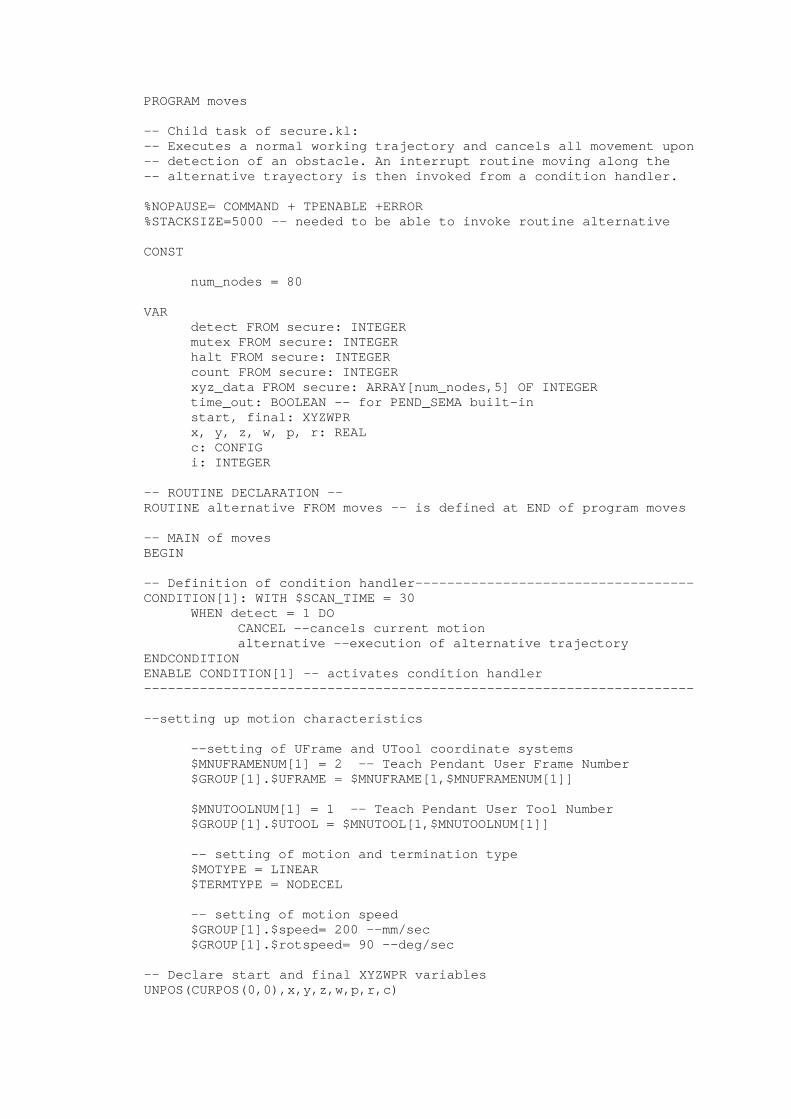
PROGRAM moves -- Child task of secure.kl: -- Executes a normal working trajectory and cancels all movement upon -- detection of an obstacle. An interrupt routine moving along the -- alternative trayectory is then invoked from a condition handler. %NOPAUSE= COMMAND + TPENABLE +ERROR %STACKSIZE=5000 –- needed to be able to invoke routine alternative CONST num_nodes = 80 VAR detect FROM secure: INTEGER mutex FROM secure: INTEGER halt FROM secure: INTEGER count FROM secure: INTEGER xyz_data FROM secure: ARRAY[num_nodes,5] OF INTEGER

time_out: BOOLEAN –- for PEND_SEMA built-in start, final: XYZWPR x, y, z, w, p, r: REAL c: CONFIG i: INTEGER -- ROUTINE DECLARATION -- ROUTINE alternative FROM moves -- is defined at END of program moves -- MAIN of moves BEGIN -- Definition of condition handler----------------------------------- CONDITION[1]: WITH $SCAN_TIME = 30 WHEN detect = 1 DO CANCEL --cancels current motion alternative --execution of alternative trajectory ENDCONDITION ENABLE CONDITION[1] -- activates condition handler --------------------------------------------------------------------- --setting up motion characteristics --setting of UFrame and UTool coordinate systems $MNUFRAMENUM[1] = 2 -- Teach Pendant User Frame Number $GROUP[1].$UFRAME = $MNUFRAME[1,$MNUFRAMENUM[1]] $MNUTOOLNUM[1] = 1 -- Teach Pendant User Tool Number $GROUP[1].$UTOOL = $MNUTOOL[1,$MNUTOOLNUM[1]] -- setting of motion and termination type $MOTYPE = LINEAR $TERMTYPE = NODECEL -- setting of motion speed $GROUP[1].$speed= 200 --mm/sec $GROUP[1].$rotspeed= 90 --deg/sec -- Declare start and final XYZWPR variables UNPOS(CURPOS(0,0),x,y,z,w,p,r,c)

start.x=250 start.y=1200 start.z=100 start.w=w start.p=p start.r=r start.config_data=c final.x=300 final.y=-700 final.z=150 final.w=w final.p=p final.r=r final.config_data=c --motion loop between final and start position WHILE detect = 0 DO MOVE TO start, WHEN detect = 1 DO CANCEL ENDMOVE IF detect = 0 THEN DELAY 1000 -- simulate operation time -- in start position ENDIF IF detect = 0 THEN MOVE TO final, WHEN detect = 1 DO CANCEL ENDMOVE ENDIF IF detect = 0 THEN DELAY 1000 -- simulate operation time -- in final position ENDIF ENDWHILE DELAY 100 -- to give moves.kl time to enter in condition handler

-- before aborting program execution. END moves -- end MAIN of moves ------------------------------------------------- -- Routine definition ROUTINE alternative CONST num_nodes = 50 VAR xyz_array: ARRAY[num_nodes] OF XYZWPR m: INTEGER x, y, z, w, p, r: REAL x_incr, y_incr, z_incr: REAL c: CONFIG x_axis, y_axis: VECTOR alpha_diff, beta_diff: REAL alpha_old, beta_old: REAL BEGIN -- Definition of x, y and z axis directions for rotational actions -- ¡¡¡MOVE ABOUT actions are defined with respect to vectors -- in the activated TOOL coordinate system!!!

-- The z axis of TOOL is the x axis of the USER Frame, -- due to the TOOL’s declaration, the y axis of TOOL is the

-- negative y axis of the USER Frame. y_axis.x=0 y_axis.y=-100 y_axis.z=0 x_axis.x=0 x_axis.y=0 x_axis.z=100 -- initialize old angle variables alpha_old=0 beta_old=0 -- Semaphore actions POST_SEMA(mutex) -- liberates comm.kl to send current TCP to MATLAB PEND_SEMA(mutex,-1, time_out) -- suspends alternative until -- first alternative positions and orientations are available -- move along alternative positions FOR m=1 TO num_nodes DO -- Rotational actions alpha_diff = xyz_data[m,4] - alpha_old beta_diff = xyz_data[m,5] - beta_old IF (alpha_diff <> 0.00) THEN WITH $TERMTYPE = NOSETTLE MOVE ABOUT x_axis BY alpha_diff alpha_old = xyz_data[m,4] --update of actual angular position ENDIF IF (beta_diff <> 0.00) THEN $TERMTYPE = NOSETTLE WITH $TERMTYPE = NOSETTLE MOVE ABOUT y_axis BY beta_diff beta_old = xyz_data[m,5] -- update of actual angular position ENDIF -- Translational actions UNPOS(CURPOS(0,0),x,y,z,w,p,r,c) xyz_array[m].x = xyz_data[m,1] xyz_array[m].y = xyz_data[m,2] xyz_array[m].z = xyz_data[m,3] xyz_array[m].w = w xyz_array[m].p = p xyz_array[m].r = r xyz_array[m].config_data = c MOVE TO xyz_array[m] NOWAIT IF (halt = 1) AND (m = count) THEN m=num_nodes –- to force a termination of the FOR loop when –- all (=count) alternative positions and rotations have been executed. ENDIF ENDFOR END alternative ----------------------------------------------------------------------

PROGRAM comm -- Child task of secure.kl, executes the following communication steps:

-- 1. Receive an obstacle detection signal from MATLAB

-- 2. Send the current robot position to MATLAB.

-- 3. Receive positional and rotational data from MATLAB. %NOLOCKGROUP %NOPAUSE= COMMAND + TPENABLE + ERROR %PRIORITY=49 CONST num_nodes = 80 VAR ComFile:FILE -- communication file for reading and writing StatCon:INTEGER -- status from Ethernet connection StatBuf:INTEGER -- status from Buffer StatCur:INTEGER -- status of set_cursor build-in StatFile: INTEGER -- status from read operations entry:INTEGER time_out: BOOLEAN -- for semaphore use BufBytes_0, BufBytes_1:INTEGER halt FROM secure: INTEGER count FROM secure: INTEGER detect FROM secure: INTEGER mutex FROM secure: INTEGER i, j, k: INTEGER num_pos: INTEGER clock_var: INTEGER x, y, z, w, p, r: REAL c: CONFIG str_x, str_y, str_z, str_w, str_p: STRING[8] index_1, index_2, index_3, index_4, index_5, index_6, index_7, index_8, index_9, index_10, index_11, index_12, index_13, index_14, index_15, index_16, index_17, index_18, index_19, index_20, index_21: INTEGER index_row: INTEGER ReadData: ARRAY[120] OF STRING[8] xyz_data FROM secure: ARRAY[num_nodes, 5] OF INTEGER -- ROUTINE DECLARATIONS ---------------------------------------------- ROUTINE start_1 BEGIN --CLOSING PORT BEFORE START MSG_DISCO('S3:',StatCon) WRITE TPDISPLAY('Disconnect Status',StatCon, CR) --SETTING FILE AND PORT ATTRIBUTES-- SET_FILE_ATR(ComFile,ATR_IA) --force reads to completion SET_VAR(entry,'*SYSTEM*','$HOSTS_CFG[3].$SERVER_PORT',2007,StatCon) --OPEN PORT-- WRITE TPDISPLAY('Opening port 2007',CR) WRITE TPDISPLAY('Listening....',CR) MSG_CONNECT('S3:',StatCon) WAIT FOR StatCon=0

WRITE TPDISPLAY('Connected',CR) --OPEN FILE FOR READ AND WRITE-- OPEN FILE ComFile ('RW','S3:') StatFile = IO_STATUS(ComFile) IF StatFile = 0 THEN WRITE TPDISPLAY('FILE=OPEN',CR) ELSE MSG_DISCO('S3:',StatCon) WRITE TPDISPLAY('Socket disconnected',StatCon,CR) ENDIF END start_1 ROUTINE start_2 BEGIN --CLOSING PORT BEFORE START MSG_DISCO('S4:',StatCon) WRITE TPDISPLAY('Disconnect Status',StatCon, CR) --SETTING FILE AND PORT ATTRIBUTES-- SET_FILE_ATR(ComFile,ATR_IA) --force reads to completion SET_VAR(entry,'*SYSTEM*','$HOSTS_CFG[4].$SERVER_PORT',2008,StatCon) --OPEN PORT-- WRITE TPDISPLAY('Opening port 2008',CR) WRITE TPDISPLAY('Listening....',CR) MSG_CONNECT('S4:',StatCon) WAIT FOR StatCon=0 WRITE TPDISPLAY('Connected',CR) --OPEN FILE FOR READ AND WRITE-- OPEN FILE ComFile ('RW','S4:') StatFile = IO_STATUS(ComFile) IF StatFile = 0 THEN WRITE TPDISPLAY('FILE=OPEN',CR) ELSE MSG_DISCO('S4:',StatCon) WRITE TPDISPLAY('Socket disconnected',StatCon,CR) ENDIF END start_2 -- END ROUTINE DECLARATIONS ------------------------------------------ --- MAIN of comm.kl -------------------------------------------------- BEGIN WRITE(CHR(128),CR)--clear user screen FORCE_SPMENU(TP_PANEL,SPI_TPUSER,1) – to activate user screen -- STEP 1: Receive detection signal ---------------------------------- start_1 -- call routine connect for server tag S3 StatFile = IO_STATUS(ComFile) clock_var=0 FOR i=1 TO 30 DO ReadData[i]='' ENDFOR BufBytes_1=0 BufBytes_0=0

--Main loop reading as long as the file status StatFile is 0 WHILE StatFile =0 DO BufBytes_0=BufBytes_0+BufBytes_1 --adjust count of

-- ReadData ARRAY --check if new data in buffer

BYTES_AHEAD(ComFile,BufBytes_1,StatBuf) IF (BufBytes_1 > 0) THEN SET_CURSOR(TPDISPLAY,9,5,StatCur) WRITE TPDISPLAY('Bytes in next package = ',BufBytes_1,CR) ENDIF --wait for first data in buffer WHILE (BufBytes_1 = 0) AND (BufBytes_0 = 0) AND (StatBuf=0) DO DISCONNECT TIMER clock_var clock_var=0 CONNECT TIMER TO clock_var BYTES_AHEAD(ComFile,BufBytes_1,StatBuf) IF (BufBytes_1=0) THEN SET_CURSOR(TPDISPLAY,7,5,StatCur) WRITE TPDISPLAY('Buffer is empty',CR) DELAY 40 -- give time to task normal to be executed ELSE SET_CURSOR(TPDISPLAY,8,5,StatCur) WRITE TPDISPLAY('Bytes in first package = ',

BufBytes_1,CR) ENDIF ENDWHILE --Reading Data out of buffer FOR i = 1 TO BufBytes_1 DO READ ComFile(ReadData[BufBytes_0+i]::1) -- ::1 forces to read -- in one byte at a time ENDFOR StatFile=IO_STATUS(ComFile) IF(ReadData[25]='0') OR (ReadData[25]='1') THEN

StatFile=1 –- forces termination of while loop if -- detection signal has entered ENDIF ENDWHILE CNV_STR_INT(ReadData[25],detect) DISCONNECT TIMER clock_var WRITE TPDISPLAY('.......',CR) WRITE TPDISPLAY('Detection = ',detect,CR) WRITE TPDISPLAY('Reading time = ',clock_var,' milliseconds',CR) -- closing communication file CLOSE FILE ComFile WRITE TPDISPLAY('Closing communication file',CR) -- END of Step 1. ----------------------------------------------------

-- STEP 2: Send current robot position to MATLAB -------------------- -- Suspending communication task until routine ALTERNATIVE in moves -- is started up: PEND_SEMA(mutex, -1,time_out) start_2 -- call routine connect for server tag S4 StatFile = IO_STATUS(ComFile) clock_var=0 WRITE(CHR(128),CR) -- clear user screen -- Register current position of Tool Center Point: UNPOS(CURPOS(0,0),x, y, z, w, p, r, c) -- Write Current position to communication port WRITE ComFile(ROUND(x)) WRITE ComFile(ROUND(y)) WRITE ComFile(ROUND(z)) StatFile=IO_STATUS(ComFile) IF StatFile=0 THEN WRITE TPDISPLAY('Writing was successfull!',CR) ELSE WRITE TPDISPLAY('Writing error...',CR) ENDIF -- Disconnect timer DISCONNECT TIMER clock_var WRITE TPDISPLAY('Writing time = ',clock_var,' milliseconds',CR) -- closing communication file CLOSE FILE ComFile WRITE TPDISPLAY('Closing communication file',CR) -- disconnecting socket MSG_DISCO('S4:',StatCon) WRITE TPDISPLAY('Disconnecting socket',CR) -- END of Step 2. ---------------------------------------------------- -- STEP 3: Read in Positional data from MATLAB ----------------------- WRITE(CHR(128),CR) -- clear user screen -- Connect ComFile to server tag S3, that is still connected: OPEN FILE ComFile ('RW','S3:') StatFile = IO_STATUS(ComFile) IF StatFile = 0 THEN WRITE TPDISPLAY('FILE=OPEN',CR) ELSE MSG_DISCO('S3:',StatCon) WRITE TPDISPLAY('ComFile not opened. Socket disconnected',

StatCon,CR) ENDIF -- Reset the counter for total number of read in positions count=0 -- Reset the halt variable of the read operations halt=0

-- Perform read operations for every package sent over socket S3. FOR i=1 TO num_nodes DO IF (i=2) THEN POST_SEMA(mutex) -- liberate moves.kl for moving

-- along alternative path ENDIF -- initializing working variables StatFile = IO_STATUS(ComFile) clock_var=0 FOR j=1 TO 120 DO ReadData[j]='' ENDFOR BufBytes_1=0 BufBytes_0=0 num_pos=0 -- indicates the number of positions in new package --Main loop reading as long as the file status StatFile is 0 WHILE StatFile =0 DO

BufBytes_0=BufBytes_0+BufBytes_1 -- adjust count of ReadData -- ARRAY

--check if new data in buffer BYTES_AHEAD(ComFile,BufBytes_1,StatBuf)

--wait for first data in buffer WHILE (BufBytes_1 = 0) AND (BufBytes_0 = 0) AND (StatBuf=0) DO DISCONNECT TIMER clock_var clock_var=0 CONNECT TIMER TO clock_var BYTES_AHEAD(ComFile,BufBytes_1,StatBuf) IF (BufBytes_1=0) AND (i>1) THEN DELAY 40 -- once the first package has been read, -- give execution time to moves.kl ENDIF ENDWHILE --Reading Data out of buffer FOR j = 1 TO BufBytes_1 DO READ ComFile(ReadData[BufBytes_0+j]::1) ENDFOR StatFile=IO_STATUS(ComFile) IF (ReadData[46]='S') OR (ReadData[67]='S')

OR (ReadData[88]='S') OR (ReadData[109]='S') THEN halt=1 ENDIF IF(ReadData[108]='0') OR (halt=1) THEN StatFile=1 ENDIF ENDWHILE

-- Update the number of positions in the package: IF (halt=0) THEN num_pos=4 count=count+4 ELSE IF (ReadData[109]='S') THEN num_pos=4

count=count+4 ELSE IF (ReadData[67]='S') THEN num_pos=2 count=count+2 ELSE IF (ReadData[88]='S') THEN num_pos=3 count=count+3 ELSE IF (ReadData[46]='S') THEN num_pos=1 count=count+1 ENDIF ENDIF ENDIF ENDIF ENDIF IF (num_pos <> 0) THEN FOR k=1 TO num_pos DO

index_1=24+(k-1)*21+1 index_2=24+(k-1)*21+2 index_3=24+(k-1)*21+3 index_4=24+(k-1)*21+4 index_5=24+(k-1)*21+5 index_6=24+(k-1)*21+6 index_7=24+(k-1)*21+7 index_8=24+(k-1)*21+8 index_9=24+(k-1)*21+9 index_10=24+(k-1)*21+10 index_11=24+(k-1)*21+11 index_12=24+(k-1)*21+12 index_13=24+(k-1)*21+13 index_14=24+(k-1)*21+14 index_15=24+(k-1)*21+15 index_16=24+(k-1)*21+16 index_17=24+(k-1)*21+17 index_18=24+(k-1)*21+18 index_19=24+(k-1)*21+19 index_20=24+(k-1)*21+20 index_21=24+(k-1)*21+21 index_row=(i-1)*4+k str_x=ReadData[index_1]+ReadData[index_2]+ReadData[index_3]+

ReadData[index_4]=ReadData[index_5] str_y=ReadData[index_6]+ReadData[index_7]+ReadData[index_8]+

ReadData[index_9]=ReadData[index_10] str_z=ReadData[index_11]+ReadData[index_12]+ReadData[index_13]+

ReadData[index_14]=ReadData[index_15] str_w=ReadData[index_16]+ReadData[index_17]+ReadData[index_18] str_p=ReadData[index_19]+ReadData[index_20]+ReadData[index_21] CNV_STR_INT(str_x,xyz_data[index_row,1]) CNV_STR_INT(str_y,xyz_data[index_row,2]) CNV_STR_INT(str_z,xyz_data[index_row,3]) CNV_STR_INT(str_w,xyz_data[index_row,4]) CNV_STR_INT(str_p,xyz_data[index_row,5])

ENDFOR DISCONNECT TIMER clock_var

WRITE TPDISPLAY('.......',CR) WRITE TPDISPLAY('Position package nº ',i,' read in.',CR) WRITE TPDISPLAY('Reading time = ',clock_var,' milliseconds',CR) ENDIF IF (halt=1) THEN i=num_nodes –- force the FOR loop to an end if string ‘S’

-- has been detected in input package ENDIF

ENDFOR -- all positions read in -- closing communication file CLOSE FILE ComFile WRITE TPDISPLAY('Closing FUZZY communication file',CR) -- END of Step 3. ---------------------------------------------------- WRITE TPDISPLAY('...',CR,'End of communication operations',CR) END comm ---------------------------------------------------------------------- -- Script of client.pl ----------------------------------------------- use IO::Socket; $socket=IO::Socket::INET->new ( PeerAddr => '193.144.187.156', PeerPort => 2008, Proto => "tcp", Type => SOCK_STREAM ) or die ("No puedo crear el Sock Cliente, CERRANDO... \n"); while($line=<$socket>) { print "$line"; } -- end of client.pl --------------------------------------------------

% MATLAB script for the execution of the FANUC active security system % Step 1: starting up the GUI CamAxis. % Return variables: % 1) Image matrices I1, I2, I3 of GICcam1, GICcam2 and GICcam3 of quiet object % 2) Ethernet socket "sock" of connection with FANUC (IP address: 193.144.187.156) at port 2007 % 3) success: is positive for successful sending of detection signal to the FANUC robot [I1,I2,I3,sock,success]=CamAxis; % Step 2: Calculating the obstacle's exact 3D position % 2.a: Search for pixel correspondences: p_corresp=correspondence(I1,I2,I3); % 2.b: Calculating 3D position of all correspondences: Pos=Pos_3D(p_corresp); % 2.c: Discarding of false correspondences and reconstructing the obstacle's position: P_obst=obst_pos(Pos); % Step 3: Receiving current Tool Center Point position string_TCP=perl('Client.pl'); P_ini=string_int(string_TCP); disp(sprintf('Current TCP position successfully received.')); % Step 4: Determination of final position P_fin_1=[300 -700 150]; P_fin_2=[250 1200 100]; dist_1=sqrt((P_ini(1)-P_fin_1(1))^2+(P_ini(2)-P_fin_1(2))^2+(P_ini(3)-P_fin_1(3))^2); dist_2=sqrt((P_ini(1)-P_fin_2(1))^2+(P_ini(2)-P_fin_2(2))^2+(P_ini(3)-P_fin_2(3))^2); if dist_1 > dist_2 P_fin=P_fin_1; else P_fin=P_fin_2; end % Step 5: Calculating alternative fuzzy path and sending it over the socket socket=fuzzy_comm(P_ini,P_fin,P_obst,sock); % ---- END of script ------ function tcp=string_int(s_tcp) % Function that converts the TCP position in string format to the integer format % ENTRY: % s_tcp: TCP position in string format % OUTPUT: % tcp: numerical TCP position tcp_x=''; tcp_y=''; tcp_z=''; num_space=0; for i=1:length(s_tcp) if s_tcp(i)==' ' num_space=num_space+1; elseif num_space==1 tcp_x=strcat(tcp_x,s_tcp(i)); elseif num_space==2 tcp_y=strcat(tcp_y,s_tcp(i)); else tcp_z=strcat(tcp_z,s_tcp(i)); end end x=str2num(tcp_x); y=str2num(tcp_y);

z=str2num(tcp_z); tcp=[x y z]; % ----- END of string_int.m -----

of ghent robot - ghent...

Documents