AD-Ai65 153 APPLICATIONS OF SPECTRAL ESTIMATION TECHNIQUES TO RADAR 1/1DOPPLER PROCESSIN..(U) NAVAL RESEARCH LAS WASHINGTON DCDRRIZNA ET AL 31 DEC 85 NRL-8958

I UNCLASIFIE F./G 17/9 MSSFEh h EE iEEEmhohmhmhhEEEu..momom

111111 0 E-18 2

IIIIg1.86

III- II25 1. 11111.6

MICROCOPY RESOLUTION TEST CHARTNATIONAL BUREAU OF STANDARDS- 1963-A

NRL Report 8950

Applications of Spectral Estimation Techniquesto Radar Doppler Processing

* Simulation and Analysis of HF Skywave Radar Data

DENNIS B. TRIZNA AND GEORGE D. McNEAL

Radar Techniques BranchRadar Division

InI-

4 In DTICU ELECTE

MARI 01986

December 31, 1985 D

NAVAL RESEARCH LABORATORY

* Washington, D.C.

Approved for public release; distribution unlimited.

6610

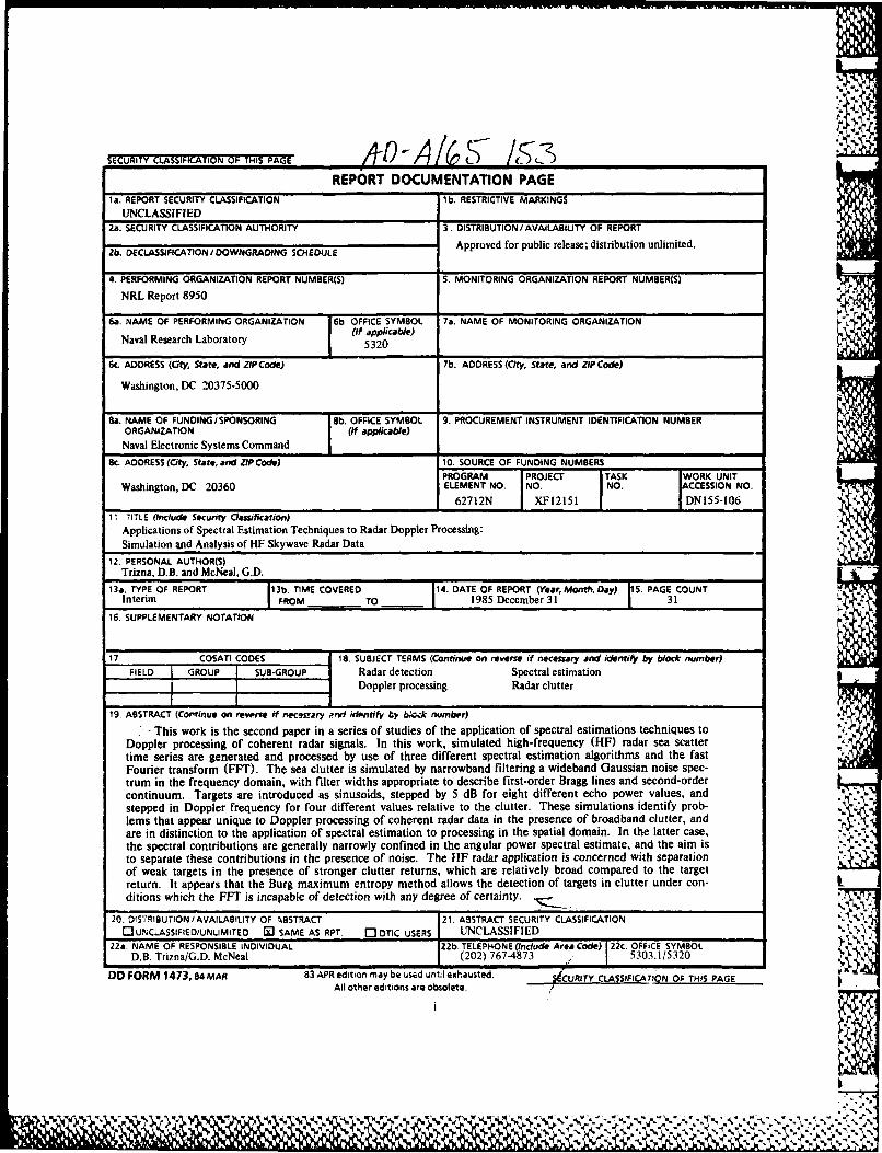
SECURITY CLASSIFICATION OF THIS PAGE AI 16 .,V 11REPORT DOCUMENTATION PAGE

la. REPORT SECURITY CLASSIFICATION lb. RESTRICTIVE MARKINGS

UNCLASSIFIED2a. SECURITY CLASSIFICATION AUTHORITY 3. DISTRIBUTION/ AVAILABIUTY OF REPORT

2b. DECLASSIFICATION/DOWNGRADING SCHEDULE Approved for public release; distribution unlimited.

4. PERFORMING ORGANIZATION REPORT NUMBER(S) S. MONITORING ORGANIZATION REPORT NUMBER(S)

NRL Report 8950

6a. NAME OF PERFORMING ORGANIZATION 6b. OFFICE SYMBOL 7a. NAME OF MONITORING ORGANIZATION

Naval Research Laboratory (if applicable)1 5320

6c. ADDRESS (City, State, and ZIP Code) 7b. ADDRESS (City, State, and ZIP Code)

Washington, DC 20375-5000

Sa. NAME OF FUNDING/SPONSORING 8b. OFFICE SYMBOL 9. PROCUREMENT INSTRUMENT IDENTIFICATION NUMBER

ORGANIZATION (If applicable)

Naval Electronic Systems Command8c. ADDRESS (Cty. State, and ZIP Code) 10. SOURCE OF FUNDING NUMBERS

PROGRAM PROJECT TASK WORK UNITWashington, DC 20360 ELEMENT NO NO. NO. ACCESSION NO.

62712N XF12151 DNI55-10611 TITLE (Include Security Classification)

Applications of Spectral Estimation Techniques to Radar Doppler Processing:Simulation vnd Analysis of HF Skywave Radar Data ?,

12. PERSONAL AUTHOR(S)

Trizna, D.B. and McNeal, G.D.

13a. TYPE OF REPORT 13b. TIME COVERED 14. DATE OF REPORT (Year, Month, Day) 5. PAGE COUNTInterim FROM TO 1985 December 31 31

16. SUPPLEMENTARY NOTATION ?,*}r

17 COSATI CODES 18. SUBJECT TERMS (Continue on reverse if necessary and identify by block number)FIELD GROUP SUB-GROUP Radar detection Spectral estimation

Doppler processing Radar clutter

19. ABSTRACT (Continue on reverse if necesrary Pnd iffentify h~. by W.k number)

'- This work is the second paper in a series of studies of the application of spectral estimations techniques to *

Doppler processing of coherent radar signals. In this work, simulated high-frequency (HF) radar sea scattertime series are generated and processed by use of three different spectral estimation algorithms and the fastFourier transform (FFT). The sea clutter is simulated by narrowband filtering a wideband Gaussian noise spec-trum in the frequency domain, with filter widths appropriate to describe first-order Bragg lines and second-ordercontinuum. Targets are introduced as sinusoids, stepped by 5 dB for eight different echo power values, andstepped in Doppler frequency for four different values relative to the clutter. These simulations identify prob-lems that appear unique to Doppler processing of coherent radar data in the presence of broadband clutter, andare in distinction to the application of spectral estimation to processing in the spatial domain. In the latter case,the spectral contributions are generally narrowly confined in the angular power spectral estimate, and the aim isto separate these contributions in the presence of noise. The HF radar application is concerned with separationof weak targets in the presence of stronger clutter returns, which are relatively broad compared to the targetreturn. It appears that the Burg maximum entropy method allows the detection of targets in clutter under con- Iditions which the FFT is incapable of detection with any degree of certainty. .I, "...

20. DISTRIBUTION /AVAILABILITY OF ,BSTRACT 21. ABSTRACT SECURITY CLASSIFICATIONOUNCLASSIFIED/UNLIMITED 111 SAME AS RPT. 0 DTIC USERS UNCLASSIFIED *\

22a. NAME OF RESPONSIBLE INDIVIDUAL 22b. TELEPHONE (Include Area Code) 22c. OFFICE SYMBOLD.B. Trizna/G.D. McNeal (202) 767-4873 I 5303.1/5320

DO FORM 1473,84 MAR 83 APR edition may be used untl exhausted. ,7URITY CLASSIFICATION OF THIS PAGEAll other editions are obsolete.

% % % %

CONTENTS

INTRODUCTION ............................................................................................. 1I

CH-ARACTERISTICS OF THE HF RADAR SEA ECHO................................................. 2

SIMULATION OF THE FIRST- AND SECOND-ORDER HF SEA ECHO ............................ 3

SIMULATION OF TARGETS IN CLUTTER .............................................................. 6

COMPARISON OF SPECTRAL ESTIMATION ALGORITHMS ON SIMULATED DATA ........ II

LIMITS OF TARGET TRACKING WITH TARGET-CLUTTER COALESCENCE.................. 18

ANALYSIS OF OTHER CLUTTER SIMULATIONS ..................................................... 18

SUMMARY ............................................................................................... 25

REFERENCES ............................................................................................ 26

Accesion

ForNTIS CRA&lDTIC TAB 3U;. announced El

Justification

By...........Dist; ibution ----------------- >

m~ ~.Avail a~id/orDit Special

fob o.l, I1

APPLICATIONS OF SPECTRAL ESTIMATION TECHNIQUESTO RADAR DOPPLER PROCESSING

SIMULATION AND ANALYSIS OF HF SKY WA VE RADAR DATA

INTRODUCTION

Spectral estimation is one useful application of autoregressive modeling by using data consisting ofa finite series of amplitude samples of an analog signal in space or time. Other applications includerobotic control and recursive digital filtering. The technique of autoregressive (AR) spectral estimationis based on developing a model for an infinite time series by using a finite set of data samples. Thus,higher spectral resolution is achieved by estimating power spectra from such a model than could beobtained by calculating the power spectra by use of traditional Fourier transform processing of the finitedata record. Spectral estimation techniques have been applied in the field of radar primarily in thespatial/ wave-nu mber domain (see, for example, Gabriel [11, for a comprehensive review of this area).Samples collected over a few-element antenna array in space are used to identify the location of strongsignals in the transform space (wave number or azimuthal angle), with much higher angular resolutionthan could be achieved with Fourier- transform processing.

Very little work has been done in the area of spectral estimation for Doppler processing ofcoherent radar data. The only work known to the authors has been a comparison of the Marple algo-rithm with fast fourier transform (FFT) processing of high-frequency (HF) radar data [21 for targets farfrom the cluiter. Only a qualitative comparison of the two techniques was made, with no quantitativeconclusions drawn. In some cases better results were observed by using a shorter number of datapoints for input into the spectral estimation algorithms than more, although Cooley [21 did not discussthe reason for this behavior. We have observed the same type of behavior in considering real data, andwe will discuss the apparent reason for this behavior in a later paper in this series.

In the second section we present a simulation of an HF radar Doppler spectrum, including bothtargets and clutter. This is accomplished by generating a time series consisting of a sinusoidal signal torepresent the target return. Two different methods are used to represent the sea clutter. The first usestwo sinusoids to represent the first-order Bragg lines; the second represents them with a very narrow-band Gaussian profile. In both cases, second-order sea clutter is represented by broader band-limitednoise in a similar manner. These narrowband noise signals are generated in the following way. Awhite-noise complex spectrum is operated on by a narrowband filter with a Gaussian profile. This isthen inverse-transformed to the time domain to represent a component of the sea clutter. An indepen-dent time series is required to represent each component of the clutter, and these are summed alongwith the target sine wave and low-level unfiltered white noise, to represent the composite time series .-

signal.

These simulated time-series data are processed by using traditional FFT techniques with long timerecords to show the "true" spectral characteristics. Then several AR spectral estimation algorithms areapplied by using much shorter time records to demonstrate the high-resolution feature of spectral esti-mation techniques, i.e., the ability to achieve the same spectral resolution as FFT processing with farfewer points. Three different methods are compared: the Burg maximum entropy method, the covari-ance method, and the autocorrelation method.

Manuscript approved June 5, 1985.

10I

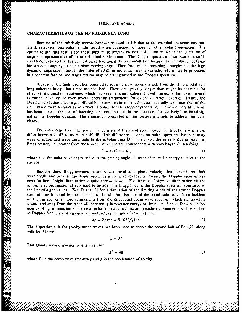
TRIZNA AND MCNEAL

CHARACTERISTICS OF THE HF RADAR SEA ECHO

Because of the relatively narrow bandwidths used at HF due to the crowded spectrum environ-ment, relatively long pulse lengths result when compared to those for other radar frequencies. Theclutter return that results for these long pulse lengths creates a situation in which the detection oftargets is representative of a clutter-limited environment. The Doppler spectrum of sea scatter is suffi-ciently complex so that the application of traditional clutter cancellation techniques typically is not feasi-ble when attempting to detect slow moving ships. Therefore, radar processing strategies require highdynamic range capabilities, in the order of 80 dB or more, so that the sea echo return may be processedin a coherent fashion and target returns may be distinguished in the Doppler spectrum.

Because of the high resolution required to separate slow moving targets from the clutter, relativelylong coherent integration times are required. These are typically longer than might be desirable foreffective illumination strategies which incorporate short coherent dwell times, either over severalazimuthal positions or over several operating frequencies for extensive range coverage. Hence, theDoppler resolution advantages offered by spectral estimation techniques, typically ten times that of theFFT, make these techniques an attractive option for HF Doppler processing. However, very little workhas been done in the area of detecting coherent sinusoids in the presence of a relatively broadband sig-nal in the Doppler domain. The simulation presented in this section attempts to address this defi-ciency.

The radar echo from the sea at HF consists of first- and second-order contributions which candiffer between 20 dB to more than 40 dB. This difference depends on radar aspect relative to primarywave direction and wave amplitude in the echoing area [3]. The first-order echo is due primarily to

a Bragg scatter, i.e., scatter from those ocean wave spectral components with wavelength L, satisfying:

L = X/ (2 cos 0), (1)

where X~ is the radar wavelength and k is the grazing angle of the incident radar energy relative to thesurface.

4 : Because these Bragg-resonant ocean waves travel at a phase velocity that depends on theirwavelength, and because the Bragg resonance is so narrowbanded a process, the Doppler resonant seaecho for line-of-sight illumination is quite narrow as well. For the case of skywave illumination via theionosphere, propagation effects tend to broaden the Bragg lines in the Doppler spectrum compared tothe line-of-sight values. (See Trizna [3] for a discussion of the limiting width of sea scatter Dopplerspectral lines imposed by the ionosphere.) In addition, because of the broad radar wave front incidenton the surface, only those components from the directional ocean wave spectrum which are traveling

* toward and away from the radar will coherently backscatter energy to the radar. Hence, for a radar fre-quency of fR in megahertz, the radar echo from approaching and receding components will be shifted

* in Doppler frequency by an equal amount, df, either side of zero in hertz:

df = 2f v/c = 0. 102 (fR). (2)

The dispersion rule for gravity ocean waves has been used to derive the second half of Eq. (2), alongwith Eq. (1) with

0 0.

This gravity wave dispersion rule is given by:f22 K (3)

where fl is the ocean wave frequency and g is the acceleration of gravity.

2

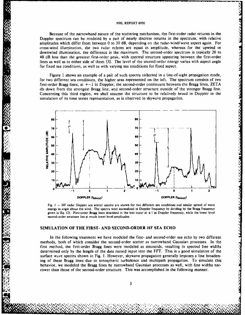
NRL REPORT 8950

Because of the narrowband nature of the scattering mechanism, the first-order radar returns in theDoppler spectrum can be modeled by a pair of nearly discrete returns in the spectrum, with relativeamplitudes which differ from between 0 to 30 dB, depending on the radar-wind/wave aspect again. Forcross-wind illumination, the two radar echoes are equal in amplitude, whereas for the upwind ordownwind illumination, the difference is the maximum. The second-order spectrum is typically 20 to40 dB less than the greatest first-order peak, with spectral structure appearing between the first-orderlines as well as to either side of them [3]. The level of the second-order energy varies with aspect anglefor fixed sea conditions, as well as with varying sea conditions for fixed aspect.

Figure 1 shows an example of a pair of such spectra collected in a line-of-sight propagation mode,for two different sea conditions, the higher seas represented on the left. The spectrum consists of twofirst-order Bragg lines, at +-I in Doppler; the second-order continuum between the Bragg lines, ZETAdb down from the strongest Bragg line; and second-order structure outside of the stronger Bragg line.Concerning this third region, we shall assume the structure to be relatively broad in Doppler in thesimulation of its time series representation, as is observed in skywave propagation.

so - -

70 00 70 7 0 - ----

'U

-so -so t:IL5

e 40 - 40 -

30 30

20 -20

10 -10

0-1 0 1 2 0-1 0 1 2

DOPPLER (fSRAGG) DOPPLER (fBRAGG)

Fig. I - HF radar Doppler sea scatter spectra are shown for two different sea conditions and similar spread of waveenergy in angle about the wind. The spectra were normalized in Doppler frequency by dividing by the Bragg frequencygiven in Eq. (2). First-order Bragg lines described in the text occur at ± I in Doppler frequency, while the lower levelsecond-order structure lies at much lower level amplitudes.

SIMULATION OF THE FIRST- AND SECOND-ORDER HF SEA ECHO

In the following treatment we have modeled the first- and second-order sea echo by two differentmethods, both of which consider the second-order scatter as narrowband Gaussian processes. In thefirst method, the first-order Bragg lines were modeled as sinusoids, resulting in spectral line widthsdetermined only by the length of the data record input into the FFT. This is a good simulation of the

6... surface Wdve spectra shown in Fig. 1. However, skywave propagation generally imposes a line broaden-ing of these Bragg lines due to ionospheric turbulence and multipath propagation. To simulate thisbehavior, we modeled the Bragg lines by narrowband Gaussian processes as well, with line widths nar-rower than those of the second-order structure. This was accomplished in the following manner.

4,..-"

% %.

TRIZNA AND MCNEAL

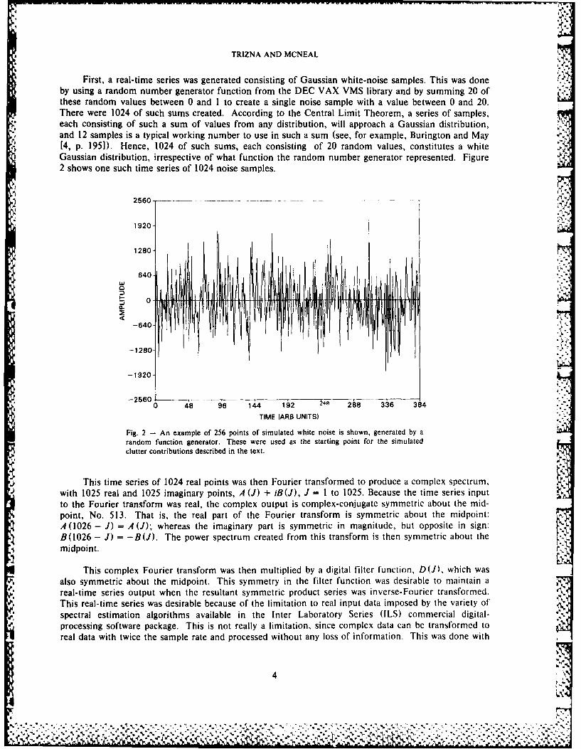
First, a real-time series was generated consisting of Gaussian white-noise samples. This was doneby using a random number generator function from the DEC VAX VMS library and by summing 20 ofthese random values between 0 and I to create a single noise sample with a value between 0 and 20.There were 1024 of such sums created. According to the Central Limit Theorem, a series of samples,each consisting of such a sum of values from any distribution, will approach a Gaussian distribution,and 12 samples is a typical working number to use in such a sum (see, for example, Burington and May[4, p. 195]). Hence, 1024 of such sums, each consisting of 20 random values, constitutes a whiteGaussian distribution, irrespective of what function the random number generator represented. Figure '6j

2 shows one such time series of 1024 noise samples.

2560 ..-- -

1920

1280-

640 -

-1280o

-1920-,

- 2560 -," - - '- -- --- -"0 48 96 144 12 8 336 384

TIME (ARS UNITS) "'

Fig. 2 - An example of 256 points of simulated white noise is shown, generated by a

random function generator. These were used as the starting point for the simulatedclutter contributions described in the text.

This time series of 1024 real points was then Fourier transformed to produce a complex spectrum, ,~with 1025 real and 1025 imaginary points, A (J) + iB(J), J = I to 1025. Because the time series input~to the Fourier transform was real, the complex output is complex-conjugate symmetric about the mid-

point, No. 513. That is, the real part of the Fourier transform is symmetric about the midpoint: iA (1026 - J) = A (J); whereas the imaginary part is symmetric in magnitude, but opposite in sign:B(1026 - J) = -B(J. The power spectrum created from this transform is then symmetric about the I:

,,, midpoint.

This complex Fourier transform was then multiplied by a digital filter function, D(J, which wasalso symmetric about the midpoint. This symmetry in the filter function was desirable to maintain areal-time series output when the resultant symmetric product series was inverse-Fourier transformed. :This real-time series was desirable because of the limitation to real input data imposed by the variety ofspectral estimation algorithms available in the Inter Laboratory Series (ILS) commercial digital- -processing software package. This is not really a limitation, since complex data can be transformed toreal data with twice the sample rate and processed without any loss of information. This was done with

V ;-, 7M-*i

~' ~ I I I]• .., -'., .- .. .". ',. : ... . ,,., .- .... ... .. . .- ., ,I .., .,I,.., -. .. I.I .- . , ., ., . , . . . .,. , . , .- . - _ . ,.-.,. ,.; -'-, ,' '., .. .;,,,'...,= .,. ,". .', '.,,., , .; ,,= .--'= .. ".. ,-..,,- .,. 2 ' .: , . .i. ,. ,':.:.---:...,.,.-..H

NRL REPORT 8950

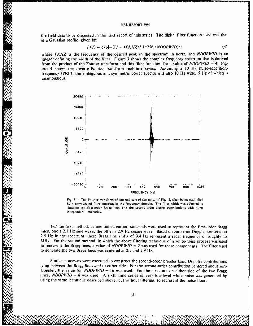
the field data to be discussed in the next report of this series. I he digital filter function used was thatof a Gaussian profile, given by:

F(J) = exp- ([J - (PKHZ/5.) *256]/NDOPWID)2} (4)

where PKHZ is the frequency of the desired peak in the spectrum in hertz, and NDOPWID is aninteger defining the width of the filter. Figure 3 shows the complex frequency spectrum that is derivedfrom the product of the Fourier transform and this filter function, for a value of NDOPWID = 4. Fig-ure 4 shows the inverse-Fourier transform real-time series. Assuming a 10 Hz pulse-repetition-frequency (PRF), the ambiguous and symmetric power spectrum is also 10 Hz wide, 5 Hz of which isunambiguous.

20480 -- ~----- ---- --

0.6015360 110240

5120-

LU

-5120

-10240-

-15360~.-20480 --

0 128 256 384 512 640 768 896 1024

FREQUENCY (Hz)

*.Fig. 3 - The Fourier transform of the real part of the noise of Fig. 2, after being multipliedby a narrowband filter function in the frequency domain. The filter width was adjusted tosimulate the first-order Bragg lines and the second-order clutter contributions with otherindependent time series.

For the first method, as mentioned earlier, sinusoids were used to represent the first-order Bragglines, one a 2.1 Hz sine wave, the other a 2.9 Hz cosine wave. Based on zero true Doppler centered at2.5 Hz in the spectrum, these Bragg line shifts of 0.4 Hz represent a radar frequency of roughly 15MHz. For the second method, in which the above filtering technique of a white-noise process was usedto represent the Bragg lines, a value of NDOPWID = 2 was used for these components. The filter usedto generate the two Bragg lines was centered at 2.1 and 2.9 Hz.

Similar processes were executed to construct the second-order broader band Doppler contributionslying between the Bragg lines and to either side. For the second-order contribution centered about zeroDoppler, the value for NDOPWID - 16 was used. For the structure on either side of the two Bragglines, NDOPWlD = 8 was used. A sixth time series of very low-level white noise was generated byusing the same technique described above, but without filtering, to represent the noise floor.

'S'S5

% % S

UL21 Ii X4

k'k S -L

TRIZNA AND MCNEAL

160 - . . . ... . ..

120

80

" 0

-80

-120 t

-1601.0 48 96 144 192 240 288 336 384

TIME (ARB UNITS)

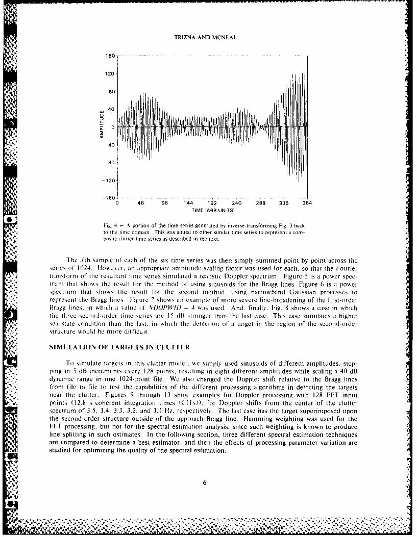
Fig 4 - A portion of the time series generated by inverse-transforming Fig. 3 backto the time domain. This was added to other similar time series to represent a com-posite Liutier time series as described in the text.

The ./th sample of each of the six time series was then simply summed point by point across theseries of 1024. iloever, an appropriate amplitude scaling factor was used for each, so that the Fourier

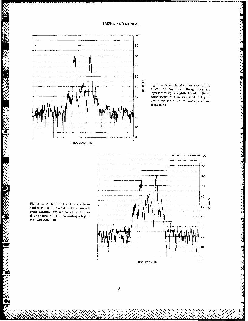
• transform of the resultant time series simulated a realistic Doppler spectrum. Figure 5 is a power spec-trum that shows the result for the method of using sinusoids for the Bragg lines. Figure 6 is a powerspectrum that shows the resu, lt for the second method, using narrowband Gaussian processes torepresent the Bragg lines. Figure 7 show, an example of more severe line-broadening of the first-orderBragg lines, in which a \,aluc of N'IDOPWID 4 was used. And. finally, Fig. 8 shows a case in whichthe tl ree second-order time series are 15 dB .,tronger than the last case. This case simulates a highersea state condition than the last, in \,hich the detet:tion o1" a target in the region of the second-orderstructure would be more difficuit.

A SIMULATION OF TARGETS IN CLUTTER

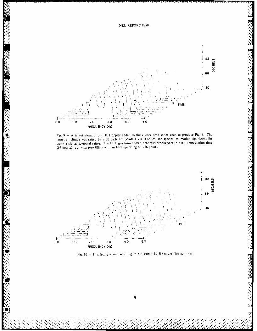
To simulate targets in this clutter model, we simply used sinusoids of different amplitudes, step-ping in 5 dB increments every 128 points, resulting in eight different amplitudes while scaling a 40 dBdynamic range in one 1024-point file. We also changed the Doppler shift relative to the Bragg linesfrom file to file to test the capabilities of the different processing algorithms in de'-cting the targetsnear the clutter. Figures 9 through 13 sho\% examples for Doppler processing with 128 FFT inputpoints (12.8 s coherent integration times ((ITs)). for Doppler shifts from the center of the clutterspectrum of 3.5, 3.4, 3.3, 3.2, and 3.1 fiz, respectively. The last case has the target superimposed uponthe second-order structure outside of the approach Bragg line. Hamming weighting was used for theFFT processing, but not for the spectral estimation analysis, since such weighting is known to produceline splitting in such estimates. In the following section, three different spectral estimation techniquesare compared to determine a best estimator, and then the effects of processing parameter variation arestudied for optimizing the quality of the spectral estimation.

~-. i. -

NRL REPORT 8950

_____100

90

'? . .. - 80

-- -- 70

.... . . . . ... 60 ,50

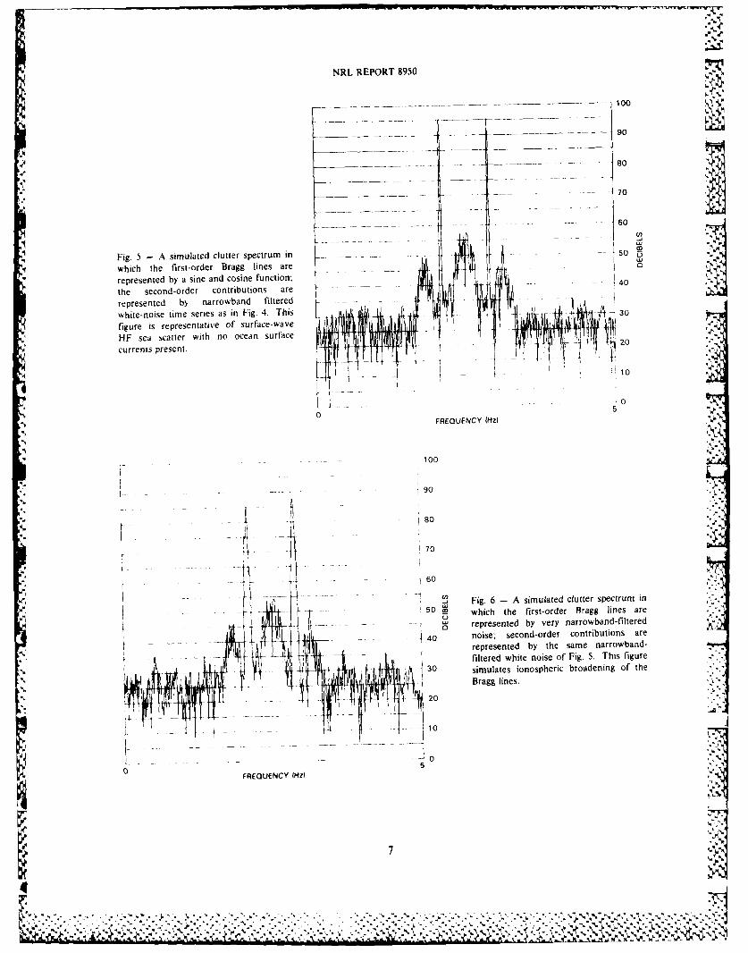
Fig. 5 A simulated clutter spectrum inwhich the first-order Bragg lines are

represented by a sine and cosine function-.:the second-order contributions are ... . - 40

represented by narrowband filteredwhite-noise time series as in Fig. 4. This 30

. figure is representative of surface-wave Idi4.

HF sea scatter with no ocean surfacecurrents present.

20

10

0 5 0

FREQUENCY (Hz)

100

80

170

*' .. - -~ - -- 9 " '

A V - 60 7

, Fig. 6- A simulated clutter spectrum in

. I. 50 T which the first-order Bragg lines are

-. represented by very narrowband-filtered

-- -40 noise; second-order contributions are

represented by the same narrowband-filtered white noise of Fig. 5. This figure

:'; ' 30 simulates ionospheric broadening of theBragg lines.

10' - , to

0 50 FREQUENCY (Hz)

%p,,

%

• L

'N. TRIZNA AND MCNEAL

- -- ----------___-- -- ---- 100

________90

- -- 70

-~ ------- --- ----- - 60

__ _ ___- ------ .--------- - - C)

- 0 Fig. 7 -A simulated clutter spectrum in50 U '

w hich the first-order Bragg lines are_______represented by a slightly broader filtered

-- 40 noise spectrum than was used in Fig. 6,simulating more severe ionospheric line

30 broadening

204,

0 5FREQUENCY (Hz)

____ ______ --- --- 100

____ _________________ ~ - 90

4% ___ ~60 lN.

Fig. 8 -A simulated clutter spectrum ------ __ __ 5 Usimilar to Fig. 7, except that the second- u

* order contrihutions are raised 10 dB rela-tive to those in Fig. 7, simulating a higher 40- -- ____

sea state condition

30

0

FREQUENCY (Hz)

8

~. ~ ~ ~ * ~. ~ '* ' .'%.,., S"-.NNNN P,

NRL REPORT 8950

92 ,

LU

66

. - - 40

-j I TIME- -T ;

7-~ -J

0.0 1.0 2.0 3.0 4.0 5.0

*FREQUENCY (Hz)

* Fig. 9 -A target signal at 3.5 Hz Doppler added to the clutter time series used to produce Fig. 6. The

target amplitude was raised by 5 dB each 128 points (12.8 s) to test the spectral estimation algorithms for

* varying clutter-to-signal ratios. The FFT spectrum shown here was produced with a 6.4-s integration time

(64 points), but with zero filling with an FFT operating on 256 points.

92 u)LU

66 4,.

9., -40

4 f.

I I TIME

00 10 20 3.0 4.0 5.0

FREQUENCY (Hz)

Fig. 10 -This figure is similar to Fig. 9. but with a 3.3 Hz target Doppler .hift

TRIZNA AND MCNEAL

92 U

-)

66

/ ill - 40

El 1 I ,~TIME

0.0 1.0 2.0 3.0 4.0 5.0

FREQUENCY (Hz)

* Fig. I1 I This figure is similar to Fig. 10, but with a 3.2 Hz target Doppler shift

92 ~

% -

40

ITIM

-17

0.0 1.0 2.0 30 4. 50

FREQUENCY (Hz)

Fig. 12 -This figure is similar to Fig. 11, but with a 3.1 Hz target Doppler shift

10

% ' * . .. 4 .

NRL REPORT 8950

".-

1 92LU

-.- ., ' I 66

, . . . .. 40_,'I

' J ' "1 II I

-I ,TIME

0.0 1.0 2.0 3.0 4.0 5.0

FREQUENCY (Hz)

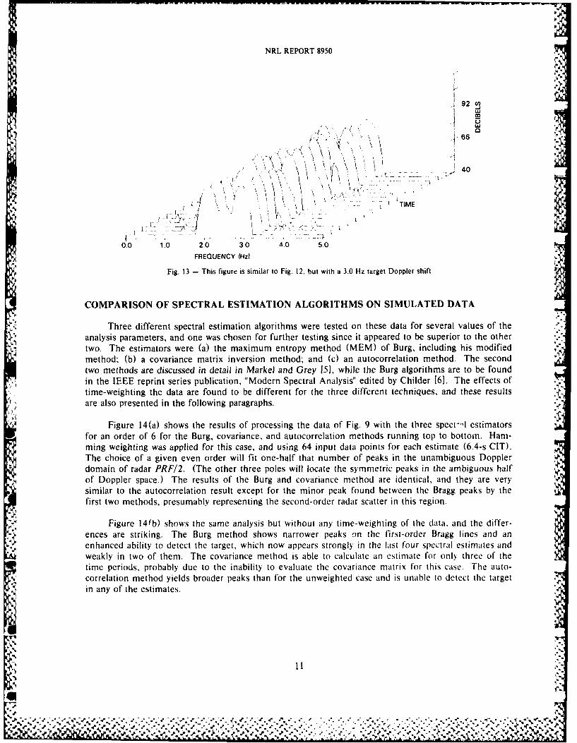
Fig. 13 - This figure is similar to Fig. 12, but with a 3.0 Hz target Doppler shift

COMPARISON OF SPECTRAL ESTIMATION ALGORITHMS ON SIMULATED DATA

Three different spectral estimation algorithms were tested on these data for several values of theanalysis parameters, and one was chosen for further testing since it appeared to be superior to the othertwo. The estimators were (a) the maximum entropy method (MEM) of Burg, including his modifiedmethod; (b) a covariance matrix inversion method; and (c) an autocorrelation method. The secondtwo methods are discussed in detail in Markel and Grey 15], while the Burg algorithms are to be foundin the IEEE reprint series publication, "Modern Spectral Analysis" edited by Childer [6]. The effects oftime-weighting the data are found to be different for the three different techniques, and these resultsare also presented in the following paragraphs.

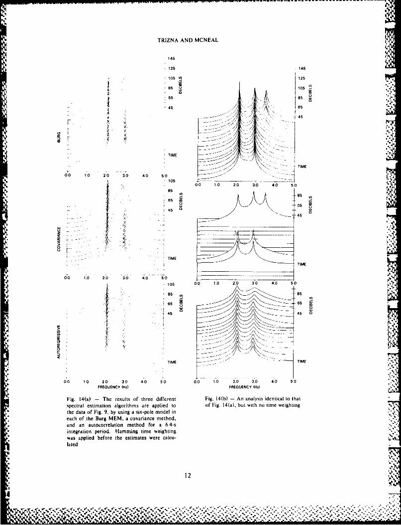
Figure 14(a) shows the results of processing the data of Fig. 9 with the three spect'- estimators ;Afor an order of 6 for the Burg, covariance, and autocorrelation methods running top to bottom. Ham-ming weighting was applied for this case, and using 64 input data points for each estimate (6.4-s CIT).The choice of a given even order will fit one-half that number of peaks in the unambiguous Dopplerdomain of radar PRF/2. (The other three poles will locate the symmetric peaks in the ambiguous halfof Doppler space.) The results of the Burg and covariance method are identical, and they are verysimilar to the autocorrelation result except for the minor peak found between the Bragg peaks by thefirst two methods, presumably representing the second-order radar scatter in this region.

Figure 14(b) shows the same analysis but without any time-weighting of the data, and the differ-ences are striking. The Burg method shows narrower peaks on the first-order Bragg lines and anenhanced ability to detect the target, which now appears strongly in the last four spectral estimates andweakly in two of them. The covariance method is able to calculate an estimate for only three of thetime periods, probably due to the inability to evaluate the covariance matrix for this case. The auto-correlation method yields broader peaks than for the unweighted case and is unable to detect the targetin any of the estimates.

d, 4%4

% - . . . . -.

TRIZNA AND MCNEAL

145

*125 145

105 125

85 10

65 185 ~45 65

F TIME -

v . . I..4TIME00 1.0 2.0 30 4.0 50so1

*10514* 0. 1.0 2.0 3.0 4.0 50

*85* 85 C

65

45

0

CTIM

TIMEE

0 0 10 20 3.0 4.0 5.01

105 0.0 1.0 2.0 3.0 4.0 5.0 11

85 ~8

'45 4

TIME TIME

00 10 2-0 30 4*0 5'0 00 __10 2__i0 3.0 4.0 50FREQUENCY (Hz) FREQUENCY (Hz)

Fig. 14(a) - The results of three different Fig. 14(b) - An analysis identical to thatspectral estimation algorithms are applied to of Fig. 14(a), but with no time weightingthe data of Fig. 9, by using a six-pole model ineach of the Burg MEM, a covariance method,and an autocorrelation method for a 6.4-sintegration period. Hamming time weightingwas applied before the estimates were calcu- L

lated.

I* 12I

NRL REPORT 8950

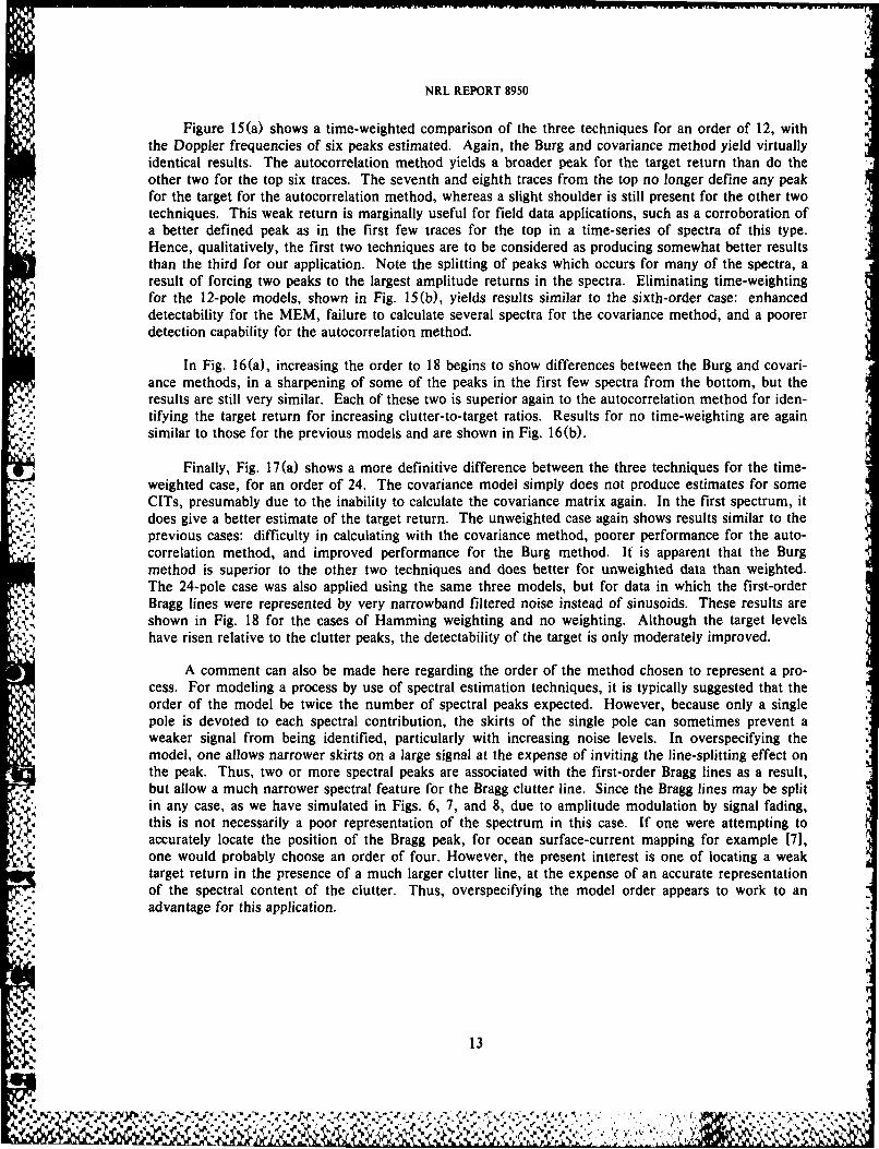
Figure 15(a) shows a time-weighted comparison of the three techniques for an order of 12, withthe Doppler frequencies of six peaks estimated. Again, the Burg and covariance method yield virtuallyidentical results. The autocorrelation method yields a broader peak for the target return than do theother two for the top six traces. The seventh and eighth traces from the top no longer define any peakfor the target for the autocorrelation method, whereas a slight shoulder is still present for the other twotechniques. This weak return is marginally useful for field data applications, such as a corroboration ofa better defined peak as in the first few traces for the top in a time-series of spectra of this type.Hence, qualitatively, the first two techniques are to be considered as producing somewhat better resultsthan the third for our application. Note the splitting of peaks which occurs for many of the spectra, aresult of forcing two peaks to the largest amplitude returns in the spectra. Eliminating time-weightingfor the 12-pole models, shown in Fig. 15(b), yields results similar to the sixth-order case: enhanceddetectability for the MEM, failure to calculate several spectra for the covariance method, and a poorer

• ,detection capability for the autocorrelation method.

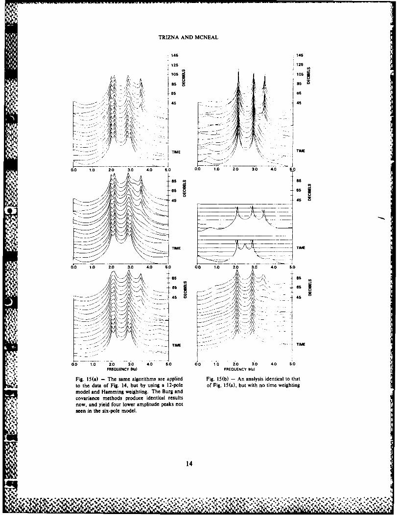
In Fig. 16(a), increasing the order to 18 begins to show differences between the Burg and covari-ance methods, in a sharpening of some of the peaks in the first few spectra from the bottom, but theresults are still very similar. Each of these two is superior again to the autocorrelation method for iden-tifying the target return for increasing clutter-to-target ratios. Results for no time-weighting are againsimilar to those for the previous models and are shown in Fig. 16(b).

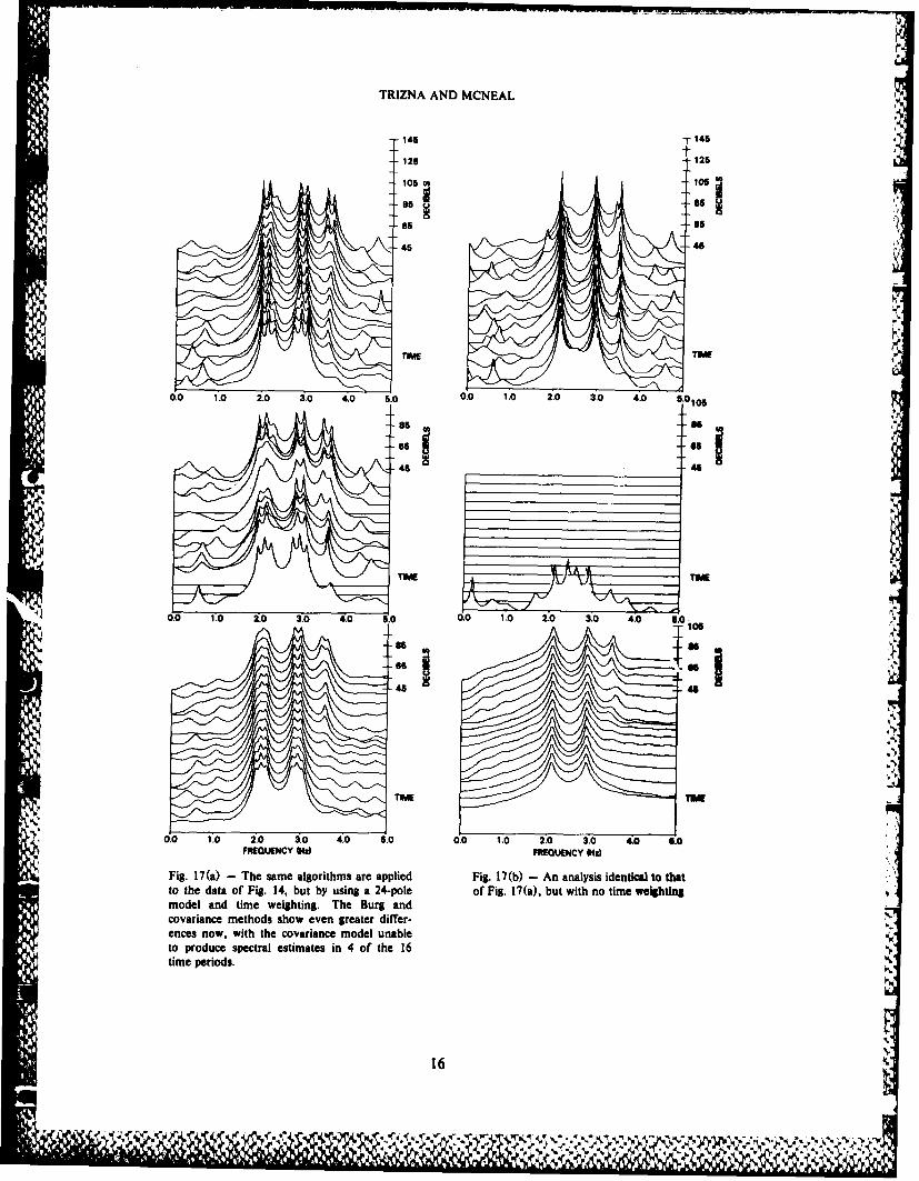
Finally, Fig. 17(a) shows a more definitive difference between the three techniques for the time-weighted case, for an order of 24. The covariance model simply does not produce estimates for someCITs, presumably due to the inability to calculate the covariance matrix again. In the first spectrum, itdoes give a better estimate of the target return. The unweighted case again shows results similar to theprevious cases: difficulty in calculating with the covariance method, poorer performance for the auto-correlation method, and improved performance for the Burg method. It is apparent that the Burgmethod is superior to the other two techniques and does better for unweighted data than weighted.The 24-pole case was also applied using the same three models, but for data in which the first-orderBragg lines were represented by very narrowband filtered noise instead of sinusoids. These results areshown in Fig. 18 for the cases of Hamming weighting and no weighting. Although the target levels

,, - have risen relative to the clutter peaks, the detectability of the target is only moderately improved.

A comment can also be made here regarding the order of the method chosen to represent a pro-cess. For modeling a process by use of spectral estimation techniques, it is typically suggested that theorder of the model be twice the number of spectral peaks expected. However, because only a singlepole is devoted to each spectral contribution, the skirts of the single pole can sometimes prevent aweaker signal from being identified, particularly with increasing noise levels. In overspecifying themodel, one allows narrower skirts on a large signal at the expense of inviting the line-splitting effect onthe peak. Thus, two or more spectral peaks are associated with the first-order Bragg lines as a result,but allow a much narrower spectral feature for the Bragg clutter line. Since the Bragg lines may be splitin any case, as we have simulated in Figs. 6, 7, and 8, due to amplitude modulation by signal fading,this is not necessarily a poor representation of the spectrum in this case. If one were attempting toaccurately locate the position of the Bragg peak, for ocean surface-current mapping for example [7],one would probably choose an order of four. However, the present interest is one of locating a weaktarget return in the presence of a much larger clutter line, at the expense of an accurate representationof the spectral content of the clutter. Thus, overspecifying the model order appears to work to anadvantage for this application.

t*.

13

N.%

TRIZNA AND MCNEAL

145 145

125 1 125

105 105

85 85

145 45/

[TIME TM

0.0 1.0 2.0 3.0 4.0 5.0 0.0 1.0 2.0 3.0 4o0 5.0

85 0 -85

as as

45 45

TIME TIME

0.0 1.0 2.0 3.0 4.0 5.0 0.0 1.0 2.0 30d 4.0 5.0

815 /V 05A IA.

__ 65 -C 5

1' 1

TIME ~..TIME

0.0 1.0 20i-- 3-.0- 4.0 5.0 0.0 1.0 2.0 3.0 4.0 5.0FREQUENCY NOi FREQUENCY (Hz)

Fig. 15(a) The same algorithms are applied Fig. 15(b) - An analysis identical to thatto the data of Fig. 14, but by using a 12-pole of Fig. 15(a), but with no time weightingmodel and Hamming weighting. The Burg andcovariance methods produce identical resultsnow, and yield four lower amplitude peaks notseen in the six-pole model.

14

IIQ

NRL REPORT 8950

146 146

1 125 15105 06

/ _ 65-~ -. ~A\ r4 '4i

0. .0 20 . 40 600 0 1.0 2.0 3.0 4.0 6.0

* 0.0 1.0 2.0 3.0 4.0 5.10. 0.1. . . . 06

85 -5

65 j545 45

00 10' 2.0 3.0 40O 5 0.0 1.0 2.0 3.0 4.0 5.0 0

FREQUENCY 04z) FREQUENCY III:

Fig. 16(a) The same algorithms are applied Fig. 16(b) - An analysis identical to thatto the data of Fig. 14, but by using an 1 8-pole of Fig. 16(a), but with no time weightingmodel and time weighting. The Burg andcovariance methods show some differencesnow, show better detection capability than the12-pole model, and are far superior to theauto-correlation model.

15

TRIZNA AND MCNEAL

145 145

12512

105j

106*95 -- as

45 46

0.0 1.0 2.0 3 .0 4.0 5.0 0.0 1.0 2.0 3.0 4.0 5

0.0 1.0 2.0 10.0 .0 0.0 1.0 2.0 3.0 40 .0 o

MNSUEWCY CHI) MFRENCY NOa

Fig. 17(a) - The same algorithms are applied Fig. 17(b) - An analysis identical to thatto the data of Fig. 14, but by using a 24-pole of Fig. 17(a), but with no time weightinmodel and time weighting. The Burg andcovariance methods show even greater differ-ences now, with the covariance model unableto produce spectral estimates in 4 of the 16time periods.

16

NRL REPORT 8950

145 146

125 125U)

15 -105

85 .4..

TIME TME

0.0 1.0 2.0 3.0 4.0 5.0 0.0 1.0 2.0 3.0 40 5.0

• -85 85

-4,. as , n

65 656

4 -45

0.0 1.0 2.0 3.0 4.0 5.0 0.0 1.0 2.0 3.0 4.0 6.0

FREQUENCY (Hz) FREOUENCY 1Hz)

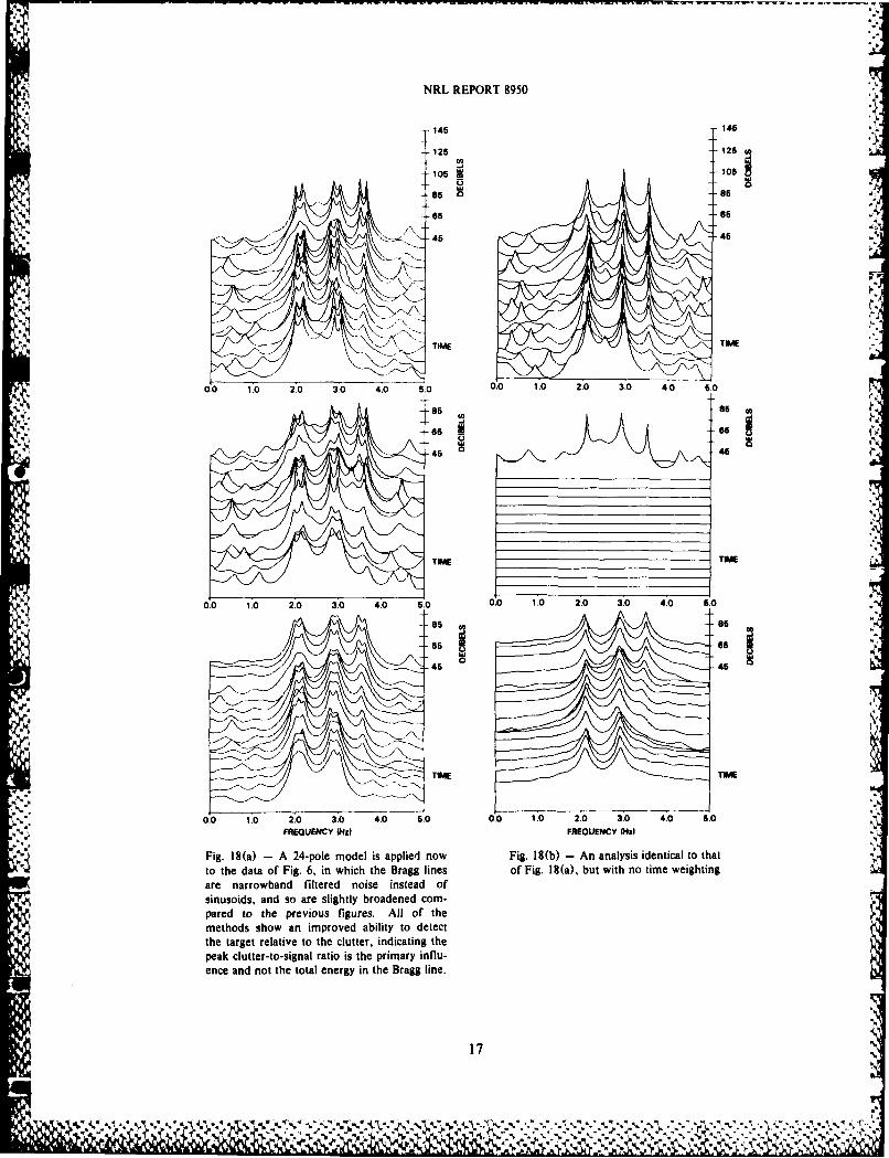
Fig. 18(a) - A 24-pole model is applied now Fig. 18(b) - An analysis identical to that

to the data of Fig. 6, in which the Bragg lines of Fig. 18(a), but with no time weighting

are narrowband filtered noise instead of

v pared to the previous figures. All of the" ' methods show an improved ability to detect

the target relative to the clutter, indicating thepeak clutter-to-signal ratio is the primary influ-

x' ence and not the total energy in the Bragg line.

178

TRIZNA AND MCNEAL

LIMITS OF TARGET TRACKING WITH TARGET-CLUTTER COALESCENCE

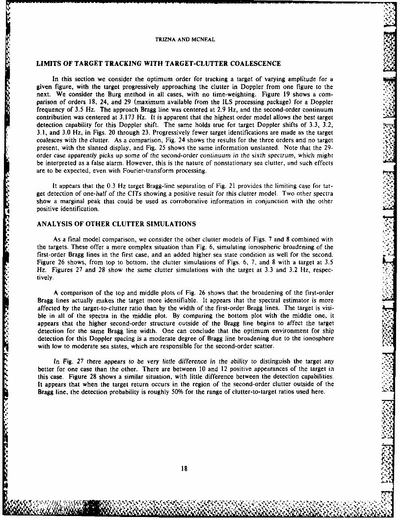
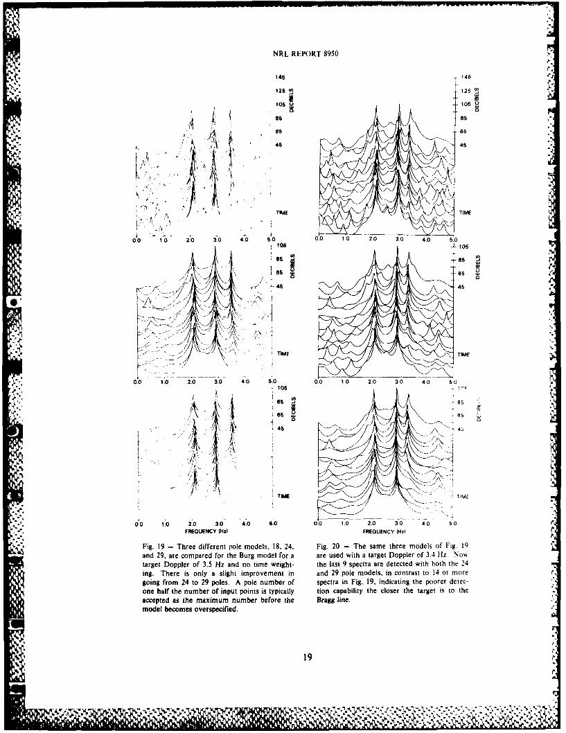
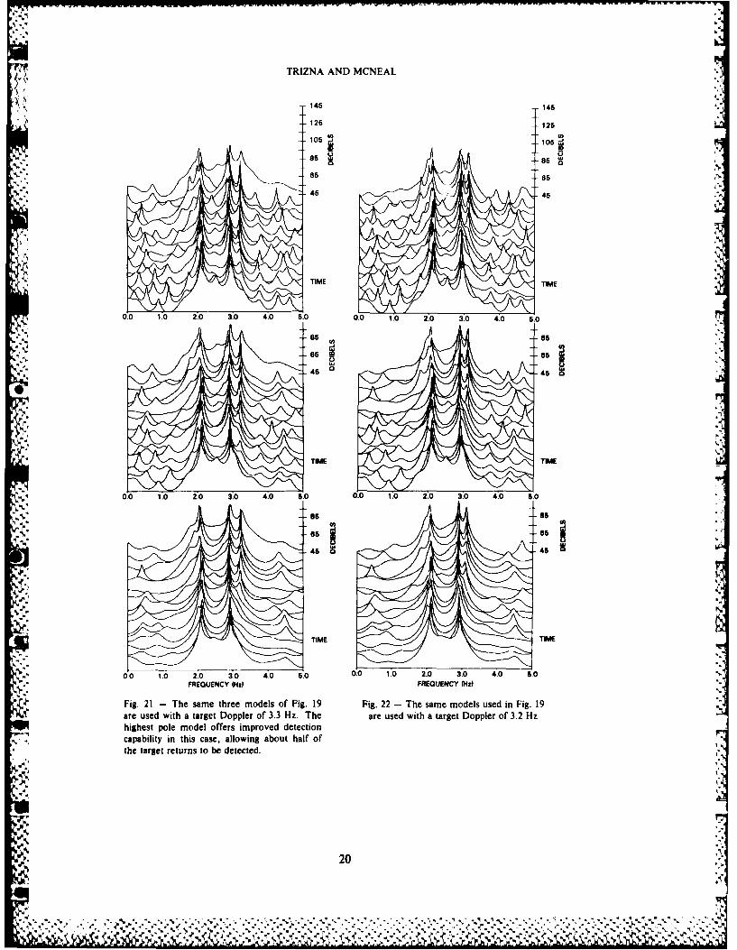
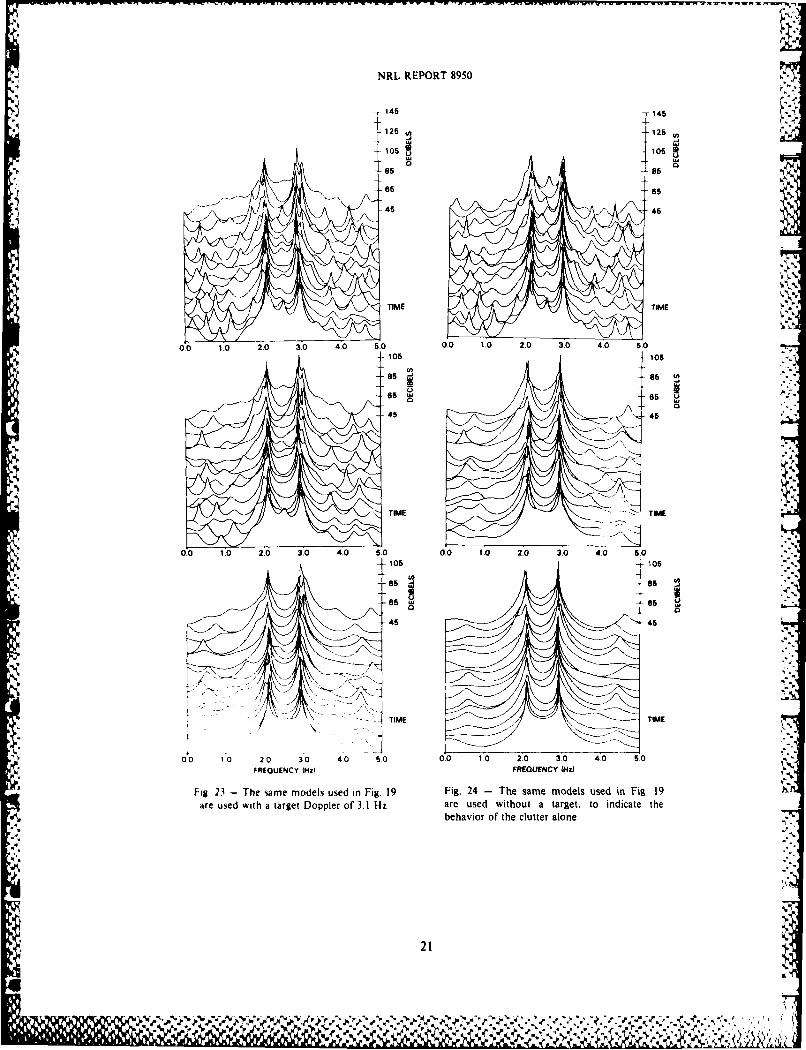
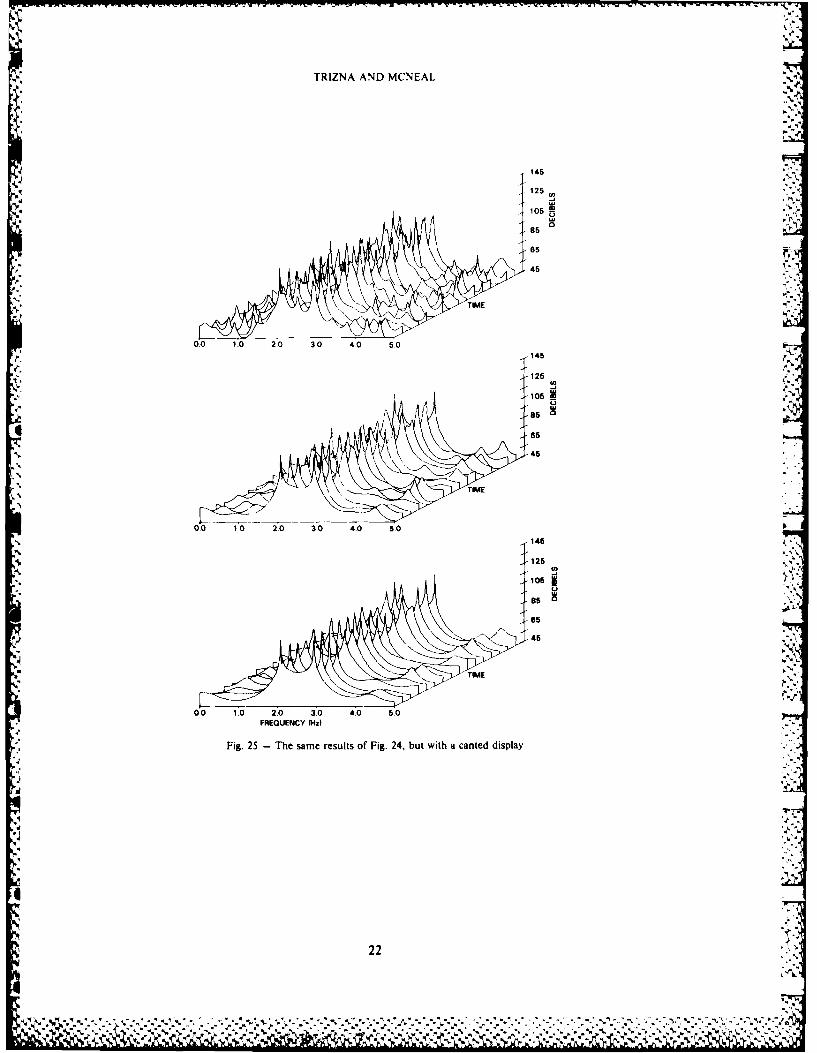
In this section we consider the optimum order for tracking a target of varying amplitude for agiven figure, with the target progressively approaching the clutter in Doppler from one figure to thenext. We consider the Burg method in all cases, with no time-weighting. Figure 19 shows a com-parison of orders 18, 24, and 29 (maximum available from the ILS processing package) for a Dopplerfrequency of 3.5 Hz. The approach Bragg line was centered at 2.9 Hz, and the second-order continuumcontribution was centered at 3.173 Hz. It is apparent that the highest order model allows the best targetdetection capability for this Doppler shift. The same holds true for target Doppler shifts of 3.3, 3.2,3.1, and 3.0 Hz, in Figs. 20 through 23. Progressively fewer target identifications are made as the targetcoalesces with the clutter. As a comparison, Fig. 24 shows the results for the three orders and no targetpresent, with the slanted display, and Fig. 25 shows the same information unslanted. Note that the 29-order case apparently picks up some of the second-order continuum in the sixth spectrum, which mightbe interpreted as a false alarm. However, this is the nature of nonstationary sea clutter, and such effectsare to be expected, even with Fourier-transform processing.

It appears that the 0.3 Hz target Bragg-line separation of Fig. 21 provides the limiting case for tar-get detection of one-half of the CITs showing a positive result for this clutter model. Two other spectrashow a marginal peak that could be used as corroborative information in conjunction with the otherpositive identification.

ANALYSIS OF OTHER CLUTTER SIMULATIONS

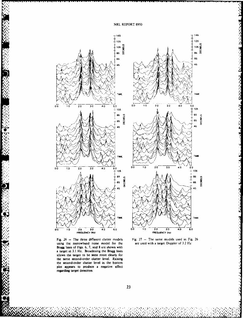
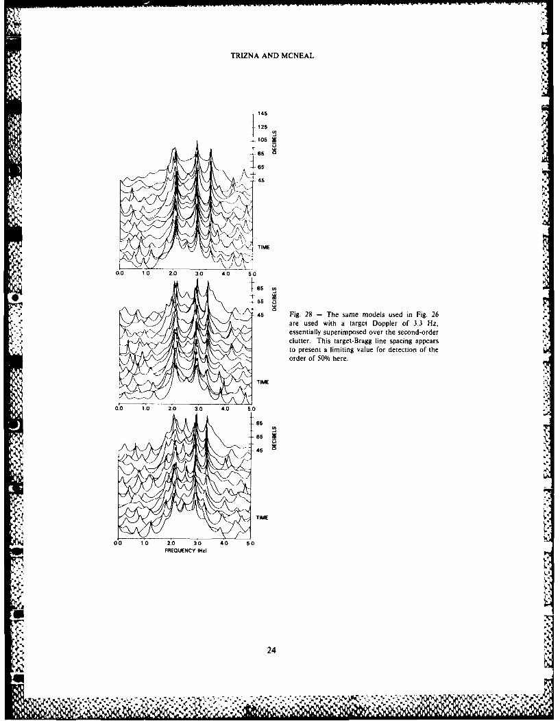
As a final model comparison, we consider the other clutter models of Figs. 7 and 8 combined withthe targets. These offer a more complex situation than Fig. 6, simulating ionospheric broadening of thefirst-order Bragg lines in the first case, and an added higher sea state condition as well for the second.Figure 26 shows, from top to bottom, the clutter simulations of Figs. 6, 7, and 8 with a target at 3.5Hz. Figures 27 and 28 show the same clutter simulations with the target at 3.3 and 3.2 LHz, respec-tively.

A comparison of the top and middle plots of Fig. 26 shows that the broadening of the first-orderBragg lines actually makes the target more identifiable. It appears that the spectral estimator is moreaffected by the target-to-cl utter ratio than by the width of the first-order Bragg lines. The target is visi-ble in all of the spectra in the middle plot. By comparing the bottom plot with the middle one, itappears that the higher second-order structure outside of the Bragg line begins to affect the targetdetection for the same Bragg line width. One can conclude that the optimum environment for shipdetection for this Doppler spacing is a moderate degree of Bragg line broadening due to the ionosphere

In Fig. 27 there appears to be very little difference in the ability to distinguish the target any

better for one case than the other. There are between 10 and 12 positive appearances of the target inthis case. Figure 28 shows a similar situation, with little difference between the detection capabilities. .-

It appears that when the target return occurs in the region of the second-order clutter outside of theBragg line, the detection probability is roughly 50%/ for the range of clutter-to- target ratios used here.

18

NRL REPORT 8950

145 145

125 125

,05 U 105

85 85

as56

-45 45

TIME TIME

0.0 10 20 30 4.0 5.0105 10

S5s1 o6 5 0 5

-46 1-45

I...." ITIME TIME r

0.0 10 20 3.0 0 5.0 00 1.0 20 30 40 50

85 8

65 854. 4

0.0 1.0 2.0 3.0 4.0 5.0 0.0 1.0 2.0 30 40 50* ~,FREOUENCY 0t4z) FREOUENCY (Hz)

Fig. 19 - Three different pole models, 18. 24, Fig. 20 - The same three models of Fig. 19and 29, are compared for the Burg model for a are used with a target Doppler of 3.4 Hz. Now%target Doppler of 3.5 H-fz and no time weight- the last 9 spectra are detected with both the 24ing. There is only a slight improvement in and 29 pole models, in contrast to 14 or moregoing from 24 to 29 poles. A pole number of spectra in Fig.. 19, indicating the poorer detec-one half the number of input points is typically tion capability the closer the target is to theaccepted as the maximum number before the Bragg line.model becomes overspecified.

19

%%A

Ra M ' "

-. ' E LL *& .....

; :::o+.o :o ,: ,:o :o 5. o~o , . .0 Io , ,

TRIZNA AND MCNEAL

~ ~146 145

126 -126

105 ios

-- 5

65 65

45 -45

TIME TIME

0.0 1.0 2.0 3.0 4.0 5.0 060 1.0 2.0 3.0 4.0 5.0

85 6-5

85 -65

45 - 45 -

TIME Tom

0.0 1.0 2'0 3.0 4.0 5.0 0.0 1.0 2.0 3.0 4.0 5.0

95 8-5

65 -65

45 45

TIME TIME

0 0 1.0 2.0 3.0 4.0 5.0 0.0 1.0 2.0 3.0 4.0 5.0FREQUENCY (HzI FREQUENCY (HO?

Fig. 21 - The same three models of Fig. 19 Fig. 22 - The same models used in Fig. 19Care used with a target Doppler of 3.3 Hz. The are used with a target Doppler of 3.2 Hz

highest pole model offers improved detectioncapability in this case, allowing about half ofthe target returns to be detected.

VV.

%2

NRL REPORT 8950

145 1451'-

125 ~'105 10

65 65

45 45

TIME TM

0.0 1.0 2.0 3.0 4.0 5.0 0.0 1.0 2.0 3.0 4.0 5.0105 0

_85 as

65a 65

_45 4

0.0 1 .0 2.0 3.0 4.0 5.0 0.0 1.0 2.0 3.0 40 5.0105 105

85 as

Co

45 4

TIME TIME

00 10 20 30 40 50 0.0 10 2.0 3.0 4.0 5.0FREGUENCY Wet FREQUJENCY (Hz)

Fig 23 - The some models used in Fig. 19 Fig. 24 - The same models used in Fig. 19are used with a target Doppler of 3.1 Hz are used without a target, to indicate the

behavior of the clutter alone

21

%I

TRIZNA AND MCNEAL

145

125

105 L

85

65

45

TI ME ,"-

O.O 1.0 2.0 30 4o 5.0 --

tF°'145

125

1105

010

45

TIME"

0O0 10 2,0 3.0 4.0 5.0

8450

4 85

45

FREQUENCY (Hz) .

-' I

Fig. 25 -- The same results of Fig. 24, but with a canted display'4,?

2212

"%%

4," V.

NRL REPORT 8950

145 1145

125 4 25

105 ~ L105 -

_85 85

- 85 65

45 '. 45

)\ \ . '" TIME . - TIME

0.0 1,0 20 30 4o0 5 0 0,0 10 2.0 30 4,0 5:0

-- 105105

65 U 0

45 46

TIME TVAE

0.0 10 2.0 30 4,0 - 5.0 0,0 1.0 20 3.0 4.0 5.0

10510

85 85 W

A 0

- 45 4

TIME TIME

00 10 2.0 30 40 s0 0.0 1,0 2.0 30 4:.0 5.0FREQUENCY (Hz) FREQUENCY (Hz)

Fig. 26 - The three different clutter models Fig. 27 - The same models used in Fig. 26using the narrowband noise model for the are used with a target Doppler of 3.2 HzBragg lines of Figs. 6, 7, and 8 are shown witha target at 3.1 Hz. Broadening the Bragg lines

* -allows the target to be seen more clearly forthe same second-order clutter level. Raisingthe second-order clutter level in the bottomplot appears to produce a negative effect

"I'd~lregarding target detection.

23

TRIZNA AND MCNEAL

145

125

_105

65

65

65 L)

45 Fig. 28 -The same models used in Fig. 26are used with a target Doppler of 3.3 Hz.essentially superimposed over the second-order

* clutter. This target-Bragg line spacing appearsto present a limiting value for detection of theorder of 50% here.

TIME

65_

_45 0

TIME

FREQUENCY HOz

t.7.

-----------------

NRL REPORT 8950

SUMMARY

In this report we have investigated the application of spectral estimation techniques to HF radarDoppler processing, with targets combined with clutter in simulated data. Several different models forthe clutter were used. In all of these, the second-order clutter contributions were modeled by a white-

42. noise spectrum operated on by a narrowband filter centered at the appropriate Doppler frequency. Forthe first type of model, the first-order Bragg lines were simulated by two sinusoids, producing very nar-row line widths. For the other models, the Bragg lines were simulated by very narrow band-limitedwhite noise to simulate line broadening by the ionosphere. Different combinations of Bragg linebroadening and ratios of first- to second-order clutter levels were simulated. Targets were included assinusoids with eight different amplitudes in a data file to study the effects of changing clutter-to-signalratios by using different spectral estimation algorithms. Different target Doppler shifts were generatedfor individual files to study the effects of target-clutter coalescence, in each case combining with identi-cal clutter data. This set of simulation models appears to provide a useful standard against which tocompare other spectral estimation techniques in future work.

Three different spectral estimation algorithms were compared for several different conditions: theBurg maximum entropy method (MEM), the covariance method, and the autocorrelation method, asdiscussed in Markel and Grey [5]. The results showed improved target detectability as model order wasincreased from 6 to 12, to 18, and finally to 24 for the Burg and autocorrelation methods. The covari-ance model was unable to provide spectral estimates for higher order models, and the Burg model wasjudged as the best of the three. Improved target detectability was found for no time weighting of thedata, in contrast to what one experiences in FFT processing.

As the target was allowed to approach the clutter in Doppler frequency, it was found that targetdetection becomes limited for cases of Doppler differences of 0.2 Hz between the target and the Braggline. For this case, only 50% of the spectra produced target detectability for the range of target-to-clutter peak simulations studied. Such a range might be representative of a fading target return col-lected via an ionospheric skywave propagation mode.

As different models of the clutter were combined with the target and processed with the Burgalgorithm for an order of 29, several interesting results appeared. First, as the Bragg line contributionswere broadened for the same noise and second-order clutter levels, the target detectability actuallyimproved. It appears that the important quantity in applying the spectral estimation algorithms is theratio of the highest clutter amplitude to the target peak, rather than the total power contained in theBragg line. This would imply that a moderate amount of ionospheric broadening actually improves thetarget detectability. Second, this held true as the second-order clutter level was increased for the same efirst-order line broadening just discussed, as long as the target was not superimposed on the second-order clutter. Finally, as the target was allowed to approach to within 0.2 Hz of the Bragg line, essen-tially lying on the second-order clutter, there appeared to be little difference between the three modelorders used as far as target detection is concerned. All three models provided the same number ofdetections.

Further work in this area of HF Doppler simulation might be fruitful in several areas. Private dis-cussions with John Shore, of NRL, indicate that application of his Cross Entropy Minimization tech-nique might be very appropriate to this problem, serving essentially as a clutter cancellation technique.The technique depends on providing a first estimate as a clutter model, then comparing this with the

., . data by including a target. As to actually employing such a technique on field data, such a comparisonmight be made of adjacent range bins, for example. Alternatively, a high spatial resolution range-azimuth cell could be compared with an average of several cells, effectively suppressing any targetspresent relative to the clutter. Moreover, the autoregressive moving-average (ARMA) models would

A_ appear on first principles to apply to this type of data, with its narrowband noise-like features, rather

25 A

,r L'AA -'

-' -

.-

TRIZNA AND MCNEAL

than the AR techniques used here that model by using poles only. The simulated data set used herewould appear to be a good standard against which to compare further. '-.

REFERENCES

[11 W.F. Gabriel, "Spectral Analysis and Adaptive Array Superresolution Techniques," Proc. IEEE 68,654-666 (1980).

[21 D.W. Cooley, "Doppler Spectral Analysis of Ship-Echo Data Collected at the WARF: A Com-parison of an Autoregressive Method to the Conventional FFT-Based Method," Technical MemoNo. 1, SRI Project 7259, June 28, 1984.

[31 D.B. Trizna, "Estimation of the Sea Surface Radar Cross Section at HF from Second-OrderDoppler Characteristics," NRL Report 8579, May 1982.

[4] R.S. Burington and D.C. May, Handbook of Probability and Statistics with Tables, 2nd ed. (NewYork, 1973).

[51 J.D. Markel and A.H. Grey, Linear Prediction of Speech (Springer-Verlag, New York. 1976).

[61 D.G. Childer, ed., Modern SpectralAnalysis (IEEE Press, New York, 1976).

[71 D.B. Trizna, "Mapping Ocean Currents Using Over-the-Horizon Radar," Int. J. Remote Sensing 3,295-309 (1982).

26-

S~ r-

-p.

5,*

DTi

IALOIXIMMLI~i- 4..