of sussex dphil thesissro.sussex.ac.uk/40673/1/simões,_armando_amorim.pdf · carlos eduardo...
TRANSCRIPT
A University of Sussex DPhil thesis
Available online via Sussex Research Online:
http://sro.sussex.ac.uk/
This thesis is protected by copyright which belongs to the author.
This thesis cannot be reproduced or quoted extensively from without first obtaining permission in writing from the Author
The content must not be changed in any way or sold commercially in any format or medium without the formal permission of the Author
When referring to this work, full bibliographic details including the author, title, awarding institution and date of the thesis must be given
Please visit Sussex Research Online for more information and further details

UNIVERSITY OF SUSSEX
The contribution of Bolsa Família to the educational achievement of economically disadvantaged children
in Brazil
Armando Amorim Simões
Thesis submitted to the University of Sussex for the degree of Doctor of Philosophy
May 2012

i
Declaration
I certify that the thesis I have presented for examination for the PhD degree in
Education of the University of Sussex is solely my own work and has not been previously
submitted to this or any other University for a degree.
The copyright of this thesis rests with the author. Quotation from it is permitted,
provided that full acknowledgement is made.
___________________________________________

ii
UNIVERSITY OF SUSSEX
ARMANDO AMORIM SIMÕES
Thesis submitted to the University of Sussex for the degree of Doctor of Philosophy
Title: The contribution of Bolsa Família to the educational achievement of economically
disadvantaged children in Brazil
SUMMARY
This study investigates effects of a conditional cash transfer programme (CCT) in Brazil – Bolsa
Família (BF) – on school outcomes, particularly children’s achievements on standardised tests, pass-grade rates, and dropout rates. The educational conditionality of the programme, requiring enrolment in school and minimum school attendance, figures as a major justification for public investment in BF. It is expected that BF will reduce short-term poverty and boost children’s human capital, thus inducing long-term socioeconomic improvement. In order to achieve its long-term objective, BF should be able to improve not only enrolment and attendance rates, but also learning outcomes and grade promotion amongst beneficiary children. However, these effects, particularly learning outcomes, have not yet been reported in the literature.
The hypothesis investigated in this thesis is that length of time of participation in the programme and per capita cash amounts received by families are key variables in assessing BF’s effects on children’s educational outcomes. As the programme improves household income, requires a high rate of school attendance, and monitors children’s health and nutritional conditions, a positive effect on children’s performance should be expected over time. Similarly, the amount of cash paid to families should have an impact on changes induced in the home environment that are beneficial for children’s educational outcomes.
Empirically, the dissertation combines three national datasets from governmental agencies for the years 2005 and 2007. These data contain information on test scores in Portuguese Language and Mathematics for fourth grade pupils, school context, and BF parameters (intake, time of participation, and cash value), which are used in cross-sectional and panel analyses to test the above hypotheses.
The results show that although beneficiaries tend to attend less well-resourced schools, the influence of individual and household characteristics on test scores overshadow that of school resources, suggesting that demand-side interventions might result in gains in children’s performances. The cross-sectional analysis at the school level suggests that BF’s contribution to school outcomes depends on the length of time of participation and the per capita cash value paid to families. In addition, these two BF parameters have substitute effects, that is, as the per capita cash increases, school performance increases; however, the contribution of time of participation to gains in school performance diminishes and vice-versa. As a sensitive analysis to test the direct effects of length of time of participation and per capita cash on school outcomes, a subsample was used, which includes only schools in which more than 80% of pupils are beneficiaries. Results from this subsample confirm the positive effects of time and cash on school outcomes, although only cash is statistically significant. Furthermore, a school-and-time fixed effects model is estimated using panel data for 2005 and 2007 for the same school outcomes. The results also suggest that improvements in school outcomes are expected over time as a result of exposure to the programme, although this varies across regions.
The findings support the idea that improvements in educational opportunities and outcomes for children of low-income families in Brazil require a non-educational policy measure – the reduction of the immediate income poverty – as intended by BF. Nevertheless, there is also an urgent need to address inequalities in standards of education supply and special attention should be given to children whose families are recipients of BF in promoting access to pre-school programmes. Even though educational policies are necessary, they are insufficient to promote human capital amongst the poorest families in Brazil. In this sense, CCTs do not represent an opportunity cost for educational policies. Instead, they are important allies in promoting education access and equity.

iii
Acknowledgments
I would like to thank the institutions whose support was invaluable over the journey of this research. The Ministry of Planning in Brazil, which granted me four years leave and funded my stay in the UK to complete this study (Oct 2008- Sep 2012); the University of Sussex, for making me a recipient of the Overseas Research Students Awards Scheme (ORSAS) during the first three years of this research; and the School of Education and Social Work, for the opportunity I had to take part in the Graduate Teaching Research Assistantship from March 2010 to July 2011.
Several people in Brazil contributed in different ways and at different moments to this research. I am grateful for the support received from my colleagues in the Ministry of Planning, especially Afonso Almeida, Amarildo Baesso, Francisco Gaetani, and Nélio Lacerda Vanderlei, over the months before my departure. I thank the staff at the Ministry of Social Development, who not only allowed me access to the Bolsa Família datasets used in this research but also supported me and this project in many other ways: Anna Claudia Pontes, Analúcia Alonso, Antonio Claret Campos, Bruno Câmara, Cláudia Regina Baddini, Cleyton Domingues, Fernando Gaiger, Fernanda Pereira de Paula, Frederico Guanais, Larissa Almeida, Leticia Bartholo, and Lucia Modesto. In the National Institute for Educational Studies and Research (INEP) I thank Carlos Eduardo Moreno, Elaine Pazello, Heliton Tavares, Liliane Lúcia Oliveira, Rafaella Cabral, and Reynaldo Fernandes, for the support and access to valuable national datasets used in this research. In the Institute for Applied Economic Research (IPEA) I would like to thank Jorge Abrahão de Castro for his support and access to micro-data from the National Household Sample Survey.
At the University of Sussex, many thanks to my supervisor, Dr. Ricardo Sabates, for his guidance, support, and friendship, as well as for the thoughtful discussions during the course of this research. I also thank Dr. Mairead Dunne for her critical comments on the final text. Finally, I would like to thank Professor Richard Dickens and Professor Barry Reilly from the Economics Department who introduced me to econometrics techniques during the autumn and spring terms of 2009/2010.
My special thanks to Caio Piza, Cecilia Ibarra, Francesca Bastagli and Sergei Soares, who kindly read drafts of this thesis and provided me with thoughtful comments and suggestions.
Finally, I am forever indebted to my wife, Carla, who has been my company, hearer, friend, and inspiration towards the end of this journey; and to my son, Tiago, who despite the physical distance took part every step of the way.

iv
Table of Contents
Chapter 1. Introduction .......................................................................................... 1
1.1 Context and Motivation ............................................................................................... 1 1.2 Purpose and Rationale ................................................................................................. 3 1.3 Questions explored and hypotheses investigated ........................................................ 4 1.4 Overview of the chapters ............................................................................................. 6
Chapter 2. Education, poverty, and inequality ........................................................ 9
2.1 Introduction ................................................................................................................. 9 2.2 The debate ................................................................................................................... 9 2.3 Does income matter for educational outcomes? ....................................................... 13
2.3.1 Theoretical models: a “mining field” ...................................................................... 13
2.3.2 Raising incomes – does it make a difference for educational outcomes? .............. 20
2.3.3 Is the evidence so far too “weak” to support policy innovation? ........................... 26
2.4 Conclusions ................................................................................................................ 28
Chapter 3. Conditional Cash Transfer Programmes: Tackling intergenerational transmission of poverty? ......................................................................................... 31
3.1 Introduction ............................................................................................................... 31 3.2 The emergence of Conditional Cash Transfer Programmes in Latin America ............. 31
3.2.1 CCTs within the social policy landscape .................................................................. 33
3.3 CCT’s long-term objective: the educational rationale ................................................ 35 3.4 The international research on CCT programmes ........................................................ 39
3.4.1 What are the effects on education? ....................................................................... 40
3.4.2 What can explain the lack of evidence of effects on learning outcomes? .............. 47
3.5 Towards the research justification ............................................................................. 50
Chapter 4. The Social and Educational Landscape in Brazil and Bolsa Família........ 53
4.1 Introduction ............................................................................................................... 53 4.2 Brazil’s social and educational context ....................................................................... 53
4.2.1 Poverty and inequality: Recent progress ................................................................ 53
4.2.2 Education access in Brazil: Successes and failures .................................................. 57
4.3 Bolsa Família programme ........................................................................................... 63
4.3.1 History and characteristics ..................................................................................... 63
4.3.2 The educational impacts of Bolsa Família: A brief review ...................................... 70
4.3.3 Programme theory ................................................................................................. 73

v
Chapter 5. Methodology, Data and Methods ........................................................ 79
5.1 Introduction ............................................................................................................... 79 5.2 Methodological issues in CCT studies ......................................................................... 79 5.3 The sources of secondary data ................................................................................... 84
5.3.1 INEP Datasets ......................................................................................................... 84
5.3.2 MDS Datasets ......................................................................................................... 86
5.3.3 The resulting datasets for analysis of Bolsa Família ............................................... 87
5.4 Research question and methods of analysis .............................................................. 88
Chapter 6. Analysing the achievement gap in Prova Brasil 2005 ........................... 93
6.1 Introduction ............................................................................................................... 93 6.2 Considerations on data, effect size, statistical power, and sample size ..................... 93
6.2.1 Data ........................................................................................................................ 93
6.2.2 The Prova Brasil proficiency scale and how to gauge differences in test scores (“effect size”) ...................................................................................................................... 96
6.2.3 Sample .................................................................................................................... 99
6.3 How do beneficiaries and non-beneficiaries compare in terms of individual, household, and school characteristics? ................................................................................ 100
6.3.1 Student Characteristics ........................................................................................ 101
6.3.2 Household Characteristics .................................................................................... 102
6.3.3 School Characteristics .......................................................................................... 103
6.4 The achievement gap between beneficiaries and non-beneficiaries ....................... 105
6.4.1 Test scores distribution and association with income .......................................... 106
6.4.2 How do test scores vary according to Bolsa Família participation taking into account specific characteristics of students, families, and schools? ................................. 111
(1) Student Characteristics and Test Scores ........................................................... 116
(2) Household Characteristics and Test Scores ....................................................... 118
(3) School Characteristics and Test Scores ............................................................. 121
6.4.3 What explains the achievement gap between beneficiaries and non-beneficiaries? . ............................................................................................................................. 122
6.5 Conclusions .............................................................................................................. 123
Chapter 7. Looking for evidence of Bolsa Família effects on school outcomes .... 126
7.1 Introduction ............................................................................................................. 126 7.2 Data and Sample ...................................................................................................... 128 7.3 Where do Bolsa Família beneficiary children study? ................................................ 131 7.4 How do schools compare as to Bolsa Família participation and observed outcomes?... ................................................................................................................................. 136 7.5 Bolsa Família factors and school outcomes .............................................................. 137

vi
7.6 The model and analysis ............................................................................................ 140
7.6.1 From the hypotheses to the econometric model ................................................. 140
7.6.2 Selecting controls for families’ and schools’ characteristics ................................. 145
7.6.3 Results (I): Testing the model ............................................................................... 149
7.6.4 Results (II): Marginal effects of BF intake on school outcomes ............................ 152
7.6.5 Results (III): Predicted Test Scores and Bolsa Família factors ............................... 161
7.6.6 Results (IV): Focusing on the 5th quintile of BF intake. ........................................ 164
7.6.6.1 Test Scores ........................................................................................................ 172
7.6.6.2 Dropout and Pass-grade rates .......................................................................... 179
7.7 Conclusions .............................................................................................................. 182 7.8 Limitations ................................................................................................................ 185
Chapter 8. Panel data analysis (2005-2007) of Bolsa Família contribution to school outcomes ......................................................................................................... 191
8.1 Introduction ............................................................................................................. 191 8.2 Panel Data of Schools ............................................................................................... 192 8.3 School outcomes, school composition, and school resources (2005-2007) ............. 195
8.3.1 School outcomes across years .............................................................................. 196
8.3.2 School composition and school resources across years ....................................... 198
8.3.3 Transitions across BF intake groups between 2005 and 2007 .............................. 201
8.4 Panel Data Model ..................................................................................................... 202 8.5 Results ...................................................................................................................... 206 8.6 Conclusions and Limitations ..................................................................................... 213
Chapter 9. Main Findings .................................................................................... 216
9.1 Introduction ............................................................................................................. 216 9.2 The achievement gap between beneficiaries and non-beneficiaries ....................... 219 9.3 The influence of Bolsa Família on school outcomes ................................................. 221 9.4 Policy implications .................................................................................................... 227 9.5 Final remarks and indications for further research .................................................. 228
REFERENCES ......................................................................................................... 231
APPENDIX Chapter 6: Tables and Graphs................................................................ 239
APPENDIX Chapter 7: Tables and Figures ............................................................... 251
APPENDIX Chapter 8 (A): Analysis of missing values for the number of Bolsa Família beneficiaries by school in 2005 .............................................................................. 261
APPENDIX Chapter 8 (B): Tables and Figures .......................................................... 274

vii
List of Tables
Table 1: School participation rate for children aged 7 to 14 by household per capita income
as fraction of minimum wage – 1992/1999 ........................................................................ 59
Table 2: Bolsa Família programme: Criteria and benefits .................................................... 68
Table 3: Number of Valid Observations for 2005 Prova Brasil Exam .................................... 95
Table 4: Proficiency scale limits and average points per month to achieve the upper limit of
the scale ........................................................................................................................... 97
Table 5: Points in test scores as percentages of one cognitive level in the proficiency scale . 97
Table 6: Test Score in Mathematics and Portuguese – 4th grade 2005 – all valid observations
......................................................................................................................................... 98
Table 7: Points in test scores as fractions of one standard deviation in observable result for
2005 ................................................................................................................................. 98
Table 8: Sample size and effect sizes (power=0.8 and alpha=.05) ........................................ 99
Table 9: Frequency distribution by Bolsa Família participation ......................................... 100
Table 10: Bolsa Família participation (2005) ..................................................................... 101
Table 11: Test Score in Mathematics and Portuguese – 4th Grade/ 2005 ............................ 106
Table 12: Average 4th grade test scores in Mathematics and Portuguese by participation in
Bolsa Família .................................................................................................................. 107
Table 13: Description of variables used to estimate Model 1 ............................................ 114
Table 14: Regression of Portuguese Test Score on STUDENT CHARACTERISTICS – 4th grade 116
Table 15: Regression of Portuguese Test Score on HOUSEHOLD CHARACTERISTICS – 4th grade
....................................................................................................................................... 119
Table 16: Regression of Portuguese Test Score on SCHOOL CHARACTERISTICS – 4th grade.. 121
Table 17: Test score gap between beneficiaries and non-beneficiaries – Portuguese 4th grade
....................................................................................................................................... 123
Table 18: Number of 4th grade schools and pupils in 2007 ................................................. 129
Table 19: Number of schools in the sample ...................................................................... 130
Table 20: Percentage of BF intake in schools (quantiles) ................................................... 132
Table 21: Pearson’s correlation coefficient between BF factors and school outcomes ....... 138
Table 22: Partial and semi-partial correlation coefficients between Portuguese Test Scores
and BF factors ................................................................................................................. 139
Table 23: Description of variables used to estimate Model 2 ............................................ 148
Table 24: Regression of test scores (Portuguese Language) on Bolsa Família factors
controlling for schools’ socioeconomic composition and resources. .................................. 150

viii
Table 25: Regression of school outcomes on Bolsa Família factors controlling for school
composition and resources. ............................................................................................. 152
Table 26: Mean and standard deviation for school outcomes and Bolsa Família factors .... 153
Table 27: Marginal effects of PropBF on school outcomes by region estimated at the mean
value of Cash and Time. ................................................................................................... 154
Table 28: Predicted Test Scores (Portuguese) by BF intake and Time of Participation in BF
(Cash=R$12.20) ............................................................................................................... 161
Table 29: Regression of school outcomes on BF factors controlling for school composition
and resources (5th quintile of BF intake) ........................................................................... 165
Table 30: Regression of school outcomes on Cash and Time (5th quintile of BF intake) ....... 166
Table 31: Hypothesis tests for effects on school outcomes ............................................... 168
Table 32: Mean and standard deviation of school outcomes and Bolsa Família factors in
schools of the fifth quintile of BF intake ........................................................................... 170
Table 33: Marginal effects of Time and Cash on school outcomes by region, estimated at the
mean values of cash and time for schools in the fifth quintile of BF intake ........................ 170
Table 34: Differences in test scores (Port) by per capita cash and variation in TIME
(NATIONAL) .................................................................................................................... 177
Table 35: Differences in test scores (Port) by time of participation and variation in CASH
(NATIONAL) .................................................................................................................... 178
Table 36: Marginal effect of Time – confidence intervals .................................................. 181
Table 37: Number of schools in the panel data ................................................................. 194
Table 38: School outcomes, school composition and school resources 2005-2007 ............. 195
Table 39: School outcomes by level of BF intake across years – 4th grade .......................... 196
Table 40: Transition table for 4th grade BF intake .............................................................. 201
Table 41: Description of variables used to estimate Model 4 ............................................ 204
Table 42: Coefficients and robust standard errors of school outcomes estimated by fixed-
effects ............................................................................................................................ 206
Table 43: Hypothesis tests for the effects of BF intake on school outcomes....................... 209
Table 44: Marginal Effect of BF intake on school outcomes by region estimated for 2005 and
2007 ............................................................................................................................... 210

ix
List of Tables (APPENDICES)
Table A - 1: Student’ characteristics (I) ............................................................................. 239
Table A - 2: Student’ characteristics (II) ............................................................................ 240
Table A - 3: Student’ characteristics (III) ........................................................................... 241
Table A - 4: Household Characteristics (I) ......................................................................... 242
Table A - 5: Household Characteristics (II) ........................................................................ 243
Table A - 6: Household Characteristics (III) ....................................................................... 243
Table A - 7: Household Characteristics (IV) ....................................................................... 244
Table A - 8: School Characteristics (I)................................................................................ 245
Table A - 9: School Characteristics (II) ............................................................................... 245
Table A - 10: School Characteristics (III) ............................................................................ 245
Table A - 11: Two-sample t-test with unequal variances for differences in Mathematics test
scores between BF and non-BF for the 4th grade ............................................................... 246
Table A - 12: Two-sample t-test with unequal variances for differences in PORTUGUESE test
scores between BF and non-BF for the 4th grade ............................................................... 246
Table A - 13: Summary statistics for household per capita income by durable goods (PNAD
2005) .............................................................................................................................. 246
Table A - 14: Students’ characteristics .............................................................................. 248
Table A - 15: Households’ characteristics ......................................................................... 249
Table A - 16: Schools’ Characteristics ............................................................................... 249
Table A - 17: Portuguese test scores and groups of characteristics (students, households and
schools) .......................................................................................................................... 250
Table A - 18: Number of schools, students, beneficiaries and students in the exam by region
....................................................................................................................................... 251
Table A - 19: Number of schools, students, beneficiaries and students in the exam by school
proportion of BF intake ................................................................................................... 251
Table A - 20: Bolsa Família characteristics by school proportion of BF intake .................... 251
Table A - 21: Bolsa Família household characteristics by school proportion of BF intake .... 252
Table A - 22: School composition as to pupils’ characteristics by school proportion of BF
intake ............................................................................................................................. 252
Table A - 23: School composition as to households’ characteristics by school proportion of BF
intake ............................................................................................................................. 252
Table A - 24: School characteristics by school proportion of BF intake (I) ........................... 253
Table A - 25: School characteristics by school proportion of BF intake (II) .......................... 253

x
Table A - 26: School outcomes by school proportion of BF intake – 4th grade 2007 ........... 253
Table A - 27: Test Scores (Portuguese) by BF intake and months of participation in the
programme ..................................................................................................................... 254
Table A - 28: Partial correlation coefficients of socioeconomic variables and school factors
with school outcomes and Bolsa Família factors (selection of controls) ............................ 255
Table A - 29: Regression of school outcomes on BF factors, school composition and school
resources. ....................................................................................................................... 256
Table A - 30: Regression of school outcomes on BF factors, school composition and school
resources for schools in the 5th quintile of BF intake ......................................................... 258
Table A - 31: Regression of test scores in MATHS on BF factors for schools in the 5th quintile
of BF intake by region...................................................................................................... 259
Table A - 32: Regression of Dropout rate on BF factors for schools in the 5th quintile of BF
intake by region .............................................................................................................. 259
Table A - 33: Mean per capita cash values at different points of the distribution by region for
schools in the 5th quintile of BF intake. ........................................................................... 260
Table A - 34: Mean time of participation at different points of the distribution by region for
schools in the 5th quintile of BF intake. ........................................................................... 260
Table A - 35: Number and percentage of missing values by original relevant variable ........ 262
Table A - 36: Number and percentage of missing values by new relevant variables ........... 263
Table A - 37: Distribution of the percentage of missing variables by students considering the
variables in Table A - 36. .................................................................................................. 264
Table A - 38: Mean, standard deviation, and quantiles of the proportion of missing values by
relevant variables across schools ..................................................................................... 265
Table A - 39: Mean, standard deviation, and quantiles of the proportion of missing values in
Q44 across schools by region ........................................................................................... 265
Table A - 40: Cross-tabulation of Q44xQ28, Pearson’s chi-square and Cramer’s V statistics 269
Table A - 41: Cross-tabulation of Q44xQ28 for school “11000201”. ................................... 270
Table A - 42: Paired t-test ................................................................................................ 271
Table A - 43: Pearson's correlation coefficient between PropBF by different methods of
adjustment ..................................................................................................................... 271
Table A - 44: Seemingly unrelated regression of Portuguese Test Scores on PropBF .......... 271
Table A - 45: Student characteristics by BF intake 2005-2007 ............................................ 274
Table A - 46: Household characteristics by BF intake 2005-2007 ........................................ 274
Table A - 47: School infrastructure by BF intake 2005-2007 ............................................... 274
Table A - 48: Class size and teachers (1st- 4th grades) by BF intake 2005-2007 ..................... 275

xi
Table A - 49: Fixed-effects regression coefficients and robust standard errors of school
outcomes on BF intake, school composition, and school resources – 4th grade. ................. 275
List of Graphs
Graph 1: Poverty Headcount Ratio and Number of Poor (1981 to 2009) .............................. 55
Graph 2: Gini coefficient for individuals’ income distribution and 10/40 income ratio (1981 to
2009) ................................................................................................................................ 55
Graph 3: School Participation Rate by Age Group (1992 to 2009) ........................................ 58
Graph 4: School Participation Rate (7 to 14) by Region (1992 to 2009) ................................ 59
Graph 5: Mean Years of Schooling by gender – Brazil (1995 to 2009) ................................... 60
Graph 6: Net Enrolment Rates in Secondary Education by Income Quintiles (2005 to 2008) . 61
Graph 7: Grade Retention and Dropout Rates in Fundamental Education (1999 to 2010) ..... 62
Graph 8: Evolution of BF cash transfers .............................................................................. 67
Graph 9: Evolution of BF participation ............................................................................... 67
Graph 10: Test Score Distribution – Mathematics 4th grade............................................... 106
Graph 11: Test Score Distribution – Portuguese 4th grade ................................................. 107
Graph 12: Mathematics test score distribution by BF participation ................................... 107
Graph 13: Portuguese test score distribution by BF participation ...................................... 108
Graph 14: Mean test scores by household goods index..................................................... 109
Graph 15: Mean test scores (Maths) by household goods index and participation in Bolsa
Família............................................................................................................................ 110
Graph 16: Mean test scores (Port.) by household goods index and participation in Bolsa
Família............................................................................................................................ 110
Graph 17: Mean Test Score by Student School History ...................................................... 112
Graph 18: Distribution of schools by percentage of BF intake ........................................... 131
Graph 19: BF indicators by groups of schools according to BF intake (%) ........................... 132
Graph 20: Students’ characteristics by BF intake (%)......................................................... 133
Graph 21: Households’ characteristics by BF intake (%) .................................................... 134
Graph 22: School Infrastructure ....................................................................................... 134
Graph 23: Teachers with higher education (%), class size and school day (min.) ................ 134
Graph 24: Mean expenditure per pupil 2008/2009 (R$) .................................................... 135
Graph 25: School achievement in test scores by BF intake (%) .......................................... 136
Graph 26: School performance indicators by BF intake (%) ............................................... 136

xii
Graph 27: Marginal Effects of BF intake on Portuguese test scores by time of participation in
BF. .................................................................................................................................. 156
Graph 28: Variation of the slope with cash value .............................................................. 158
Graph 29: Variation of the slope with time of participation .............................................. 159
Graph 30: Predicted Test Scores (Portuguese) for one and four years of participation in BF.
....................................................................................................................................... 163
Graph 31: Marginal Effects of CASH on Portuguese Test Scores ........................................ 172
Graph 32: Marginal Effects of TIME on Portuguese Test Scores ......................................... 172
Graph 33: Marginal effect of CASH on DROPOUT rate....................................................... 179
Graph 34: Marginal effect of TIME on DROPOUT rate ....................................................... 180
Graph 35: Marginal effect of CASH on PASS-GRADE rate................................................... 181
Graph 36: Marginal effect of TIME on PASS-GRADE rate ................................................... 181
Graph 37: Mean Test Score in PORTUGUESE 2005-2007 .................................................... 197
Graph 38: Mean Test Score in MATHS 2005-2007 ............................................................. 197
Graph 39: Mean Pass-grade rate 2005-2007 ..................................................................... 197
Graph 40: Mean Dropout rate 2005-2007 ......................................................................... 198
List of Graphs (APPENDICES)
A- Graph 1: Mean Household Income Per Capita by Durable Goods (PNAD 2005) .............. 246
A- Graph 2: Mean test score (Port) by students’ demographic characteristics ................... 247
A- Graph 3: Mean test score (Port) by students’ habits and expectations .......................... 247
A- Graph 4: Mean test score (Port) by households’ material environment......................... 247
A- Graph 5: Mean test score (Port) by households’ learning environment ......................... 247
A- Graph 6: Mean test score (Port) by family structure ..................................................... 247
A- Graph 7: Mean test score (Port) by parents’ characteristics .......................................... 247
List of Figures Figure 1: Economic framework .......................................................................................... 14
Figure 2: Mayer’s heuristic income model .......................................................................... 16
Figure 3: Comprehensive economic framework .................................................................. 17
Figure 4: Ecological framework .......................................................................................... 19
Figure 5: Human capital rationale ...................................................................................... 36
Figure 6: Attainment profiles for ages 15 to 19, by economic group: Mali and Brazil............ 63

xiii
Figure 7: Socio-educational rationale of Bolsa Família ........................................................ 75
Figure 8: Marginal Effects of BF intake on Portuguese test scores by time of participation at
different percentiles of per capita Cash. ........................................................................... 157
Figure 9: Predicted Test Scores (Portuguese) for different periods of participation in BF. .. 162
Figure 10: Assumption behind cross-sectional comparison. .............................................. 188
Figure 11: Potential bias in cross-sectional comparison. ................................................... 189
Figure 12: Double difference estimation .......................................................................... 190
Figure 13: Hypothesis of diminishing marginal effect of BF intake on school outcome (Y) .. 208
Figure 14: Marginal effects of BF intake on school outcomes by year (NATIONAL) ............. 210
Figure 15: Marginal effects of time on school outcomes by level of BF intake (NATIONAL) 212
List of Figures (APPENDICES) Figure A- 1: Marginal Effects of BF intake on Portuguese test scores by per capita cash at
different percentiles of Time. .......................................................................................... 257
Figure A- 2: Marginal effects of BF intake on test scores (Portuguese) by region................ 276
Figure A- 3: Marginal effects of BF intake on pass-grade rates by region ........................... 276
Figure A- 4: Marginal effects of BF intake on dropout rates by region ............................... 276
Figure A- 5: Marginal effects of BF intake on test scores (Mathematics) by region ............. 277

1
Chapter 1. Introduction
1.1 Context and Motivation
Amongst the universal basic human rights, education has been recognised as a
pathway to broaden freedoms and to empower individuals and societies; as a main vehicle to
promote culture, knowledge, and social values; and as a strategic provider of benefits to other
dimensions of social and human development. Education has also been captured as a key
element within the machinery of capitalism to produce functioning citizens for the productive
system and to promote prosperity and wealth amongst individuals, families, and society.
Simultaneously and contradictorily, education can reinforce social exclusion, marginalisation,
and segregation amongst individuals and social groups by means of its social and institutional
organisation, including its system of provision and delivery through schools and school
systems. Particularly for socioeconomically disadvantaged groups, failure in providing equality
of educational opportunities can compromise children’s expectations for a future free of
poverty and deprivation. Failures in policy equity can occur not only through deficiencies in
coverage or quality of educational services delivered, but also by the initial socioeconomic
conditions of children. Initial conditions render individuals unequal in their ability to
participate in public policies and to convert public services into real benefits. This makes
policies focused on social disadvantage important in achieving the basic universal right to
education.
The fundamental contradiction raised above derives from the fact that education can
reproduce social stratification through several institutional and social mechanisms. Education
is also a powerful means through which children from disadvantaged families are expected to
overcome initial social inequalities and access better opportunities in life. In order to achieve
the latter, social policies and education systems must act to counterbalance the initial
inequalities children bring to school. Creating educational opportunities is not enough. It is
essential to know how social conditions interact to produce children’s educational outcomes
and, thus, which policies and programmes are most effective in achieving greater educational
equality.
The general focus of this study is the relationship between family income and
educational outcomes, and the role that Bolsa Família (BF) – a conditional cash transfer (CCT)
programme for education, nutrition, and health care in Brazil – can play in developing a more

2
conducive environment for children’s educational outcomes, and thus to contribute to low-
income children’s education. In particular, this study investigates whether BF has any effect on
children’s learning outcomes, measured through achievement in standardised test scores, and
whether length of time of participation in the programme and the value of per capita cash
transfers to families are influential in the educational outcomes of beneficiary children.
The motivation for this research is interwoven with my work experience over the last
20 years as public policies manager in the fields of education, planning, and evaluation both at
local and national levels in Brazil. At the time the first local CCTs were being implemented in
Brazil (1995), I worked as planning director in the Secretariat of Education in Angra dos Reis
municipality (state of Rio de Janeiro) during the second Workers’ Party administration in the
town. In 1998, as planning advisor in the Mayor’s Cabinet, I started studying the different
experiences of CCTs implemented across the country (which at that time were conditional on
education only) as to their objectives, design, and strategy of implementation. In 1999, as
Secretary of Education, I started the political process of creating the municipal Bolsa Escola
programme in Angra dos Reis, which became a municipal law and was implemented in
2000/2001.
In 2001 I was based in Brasília. This was the year that the Federal Government
launched the National Bolsa Escola programme, covering more than three thousand
municipalities in its first year of implementation. Between 2001 and 2002 I worked as a
coordinator in the newly created National Secretariat of the Bolsa Escola Programme in the
Ministry of Education, where I framed the programme’s evaluation plan and a proposal for a
school attendance system that would allow control of the conditionalities attached to Bolsa
Escola. In 2002 I pursued a Master’s Degree at the London School of Economics in the UK,
where I studied the limitations of the monetary approach to defining the operational concept
of poverty used in the federal Bolsa Escola programme to identify and select beneficiaries.
Back in Brazil, in 2004, while working as director of educational projects in the Ministry of
Education, I maintained close cooperation with colleagues who started working in the Ministry
of Social Development on the new flagship programme in Luiz Inácio Lula da Silva’s
government – Bolsa Família. In 2007 I worked in the Ministry of Planning as director of the
Multi-year Plan, when the challenges of evaluating large-scale government programmes
became clear to me. The plan of retreating again for a period of study, in which I could engage
in the evaluation of a large-scale programme, was made possible in 2008; a natural candidate
was the BF programme.

3
By the time I left for my doctoral studies at the University of Sussex (UK), BF had
already reached full coverage and was the most popular social programme in Brazil, gaining
further momentum in the second term of Lula’s presidency. At the same time, the Ministry of
Education had already conducted two national rounds of the new School Performance
National Assessment (Prova Brasil 2005 and 2007). These new achievement indicators at the
school level could be used to assess the potential contributions of BF to beneficiaries’ learning
outcomes. Despite the success of CCTs in increasing enrolment and attendance rates for
children of low-income families, the efficacy of CCTs in promoting long-term poverty reduction
by keeping children in school was under attack.
A paper commissioned by UNESCO triggered my interest in the subject. Entitled
“Where is the ‘education’ in conditional cash transfers in education?” (Reimers, Silva and
Trevino, 2006), the paper unleashed fierce criticism of CCTs based on the lack of evidence that
these programmes could, in fact, have an impact on the learning outcomes, promotion, and
completion rates of beneficiaries. Given the impoverished conditions of schools generally
attended by beneficiaries, the authors argue that CCTs represent a double opportunity cost in
terms of education policy. First, CCTs use proportionally high shares of the national education
budget in many countries, diverting resources that could be applied to better educational
opportunities for socioeconomically disadvantaged children. Second, governments move away
from necessary educational reforms and justify investment in human capital by investing in
cash transfers conditional on education — a policy that is both easy to implement and that is
electorally attractive. In my view, the argument is valid but it misses the point that poverty has
an impact on the possibility of education for disadvantaged children. This is not only or
necessarily due to the lack of provision of quality schools, but is because of the impact poverty
has on the capacity of children to participate in education policies and to convert educational
services into real benefits. In this sense, educational policies should be complemented by
social policies focused on the conditions of low-income households and their capacity to
support children’s education. CCTs represent an alternative means to achieve that goal.
1.2 Purpose and Rationale
Conditional cash transfer programmes were developed based on the assumption that
they could contribute to poverty relief in the short term and promote human capital
accumulation in the long term, thus rescuing future generations from the “poverty trap”. Due
to budget limitations, cash transfers have not always worked as a minimum income policy, but
instead as an incentive to change families’ behaviour in favour of their children’s futures as

4
long as education, health care, and nutrition are regarded. However, if CCTs have no impact on
learning outcomes, grade progression, and completion rates for beneficiary children, then
their educational justification beyond a mere short-term incentive for school attendance might
be compromised. The strength of political support for CCTs comes mainly from the
‘educational promises’ the policy makes to families with respect to their children’s futures and
to society as a whole in fighting structural causes of poverty in developing countries.
Recognised impacts on short-term poverty alleviation, although significant, cannot sustain
changes in the long term so that children can achieve a future different from that of their
parents. CCT programmes are expected to interfere with family dynamics by changing
behaviours towards children’s time allocation for school and work, and by improving school
attendance and children’s nutritional and health conditions. Therefore, CCTs should have a
significant impact on human capital accumulation in the long term.
Amongst the educational outcomes studied with respect to CCT programmes, learning
has so far been the least contemplated, although this outcome is probably the most significant
in linking present and future poverty. This research makes its contribution by investigating test
score achievement, making use of new datasets available in Brazil, which include students’ test
scores in Mathematics and Portuguese Language as well as socioeconomic and school
variables. This research also benefits from the national coverage of databases collected from
government agencies allowing for a nation-wide analysis, thereby enlarging the scope of
previous studies of CCT programmes in Brazil. Another positive aspect is the time period this
study covers. So far, most studies focused on learning outcomes have analysed CCT
programmes in their very early stages, not allowing for the accumulations this kind of policy
may require in producing any significant effect on students’ learning outcomes. BF was
initiated in 2003, following its predecessor Bolsa Escola (2001). Two rounds of national
examinations (2005 and 2007) are used in this research to assess potential effects on school
outcomes. Differences in mean test scores, and pass-grade and dropout rates are analysed
across time at the school level, accounting for differences in the length of time of exposure to
the programme and to differences in cash amounts paid to families in each school.
1.3 Questions explored and hypotheses investigated
The main research question investigated in this thesis is whether Bolsa Família makes
any positive contribution to the educational outcomes of economically disadvantaged children,
particularly to the achievement in national standardised exams. In investigating that question,
several other interesting issues are explored before I delve into the empirical analysis. First,

5
why should family income influence children’s learning? What mechanisms interfere with the
educational opportunities and outcomes of children of low-income families? Even if one
agrees that income makes a difference, does this mean that by raising the incomes of families,
children will benefit from better results at school? Is there any evidence in the literature of the
income effect on educational outcomes, or of the impact of anti-poverty or welfare
programmes on children’s performance at school? These questions interrogate how and why
income affects children’s outcomes and why poverty potentially undermines educational
opportunities, shedding some light on the potential contribution of anti-poverty and welfare
programmes to protecting the right to education.
A second set of issues emerges by asking what it is about CCT programmes that link
this type of policy to the educational opportunities of low-income children. Is there any
educational rationale behind CCT programmes? Why should we expect any effect of CCTs on
educational opportunities and outcomes? What has research so far revealed about the
significance of these programmes to the educational opportunities and outcomes of children
of poor families? Can we expect children to escape from future poverty by taking part in CCT
programmes? These questions put CCT programmes in perspective with respect to the long-
term objectives claimed by policy-makers that human capital accumulation is a desired and
achievable goal of CCTs.
A third set of issues brings us to the Brazilian social and educational context. Why were
CCTs such as Bolsa Escola and Bolsa Família proposed in Brazil in the first place? How has the
recent evolution of access to basic education in Brazil justified these initiatives? How has BF
evolved, what are its main characteristics, and how does it intend to tackle the
intergenerational transmission of poverty? What is the theory behind the programme that can
justify such a long-term objective? Is there any research-based evidence of the educational
impacts of BF? By understanding the programme’s theory and how it is designed to create a
more conducive environment for children’s education in the present, the critical pathways
towards children’s life chances in the future can be identified. Based on these pathways,
hypotheses of BF’s potential effects on education can be tested, amongst them, the
contribution to learning outcomes. This leads back to the main question raised at the outset of
this section and to the core set of empirical questions investigated in this study.
In asking whether BF makes any positive contribution to the educational outcomes of
economically disadvantaged children, I consider potential effects on achievement in test
scores and in pass-grade and dropout rates. In the first part of the analysis I start by examining
how beneficiaries and non-beneficiaries differ. What are the conditions of the home

6
environments in which children live? What kind of support do they have from parents? What
expectations do they hold for the future? I also investigate the conditions of their schools and
what kinds of experiences they have had in those schools. Finally, I examine how children
perform on the national examination and investigate what can explain eventual differences in
test score achievements between beneficiaries and non-beneficiaries.
Differences in performance between beneficiaries and non-beneficiaries are reflected
in the mean test scores achieved in each school, as well as in other performance indicators
such as pass-grade and dropout rates. In the second part of the analysis I look at those
differences across schools vis-à-vis the BF factors (BF intake, length of time of participation,
and per capita cash amounts). Do time of exposure to BF and per capita cash paid to families in
each school positively influence school results and reduce the gap between high-BF-intake
schools and low-BF-intake schools? If yes, can the positive effect on school outcomes be
attributed to improvements in beneficiaries’ educational outcomes? The main hypotheses I
test are that BF effects educational outcomes depending on the length of time of exposure to
the programme and on the relative cash value paid to families. These factors potentially
interact with each other and moderate the effect of BF intake in each school, possibly
revealing positive effects of BF on school outcomes.
Schools also change over time in terms of composition, resources, and outcomes, as
well as in terms of BF factors. In the third part of the empirical analysis I look at changes that
occurred between 2005 and 2007: did school outcomes improve between 2005 and 2007? If
yes, can that improvement to some extent be associated with the level of BF participation in
each school, independent of eventual changes in school resources and composition?
These are the questions at the heart of this thesis for which I offer answers over the
forthcoming chapters.
1.4 Overview of the chapters
The remainder of this thesis comprises eight chapters. In chapter two I briefly describe
the academic debate concerning the relationship between poverty and education, and how
the mutual influences of socioeconomic background and school conditions on children’s
outcomes have been considered over the last decades. The question of whether and why
family income might matter to children’s outcomes is considered through the lenses of four
theoretical syntheses about that relationship. This is followed by a review of some of the
empirical evidence of whether anti-poverty and welfare programmes involving cash transfers

7
to poor families have any impact on educational outcomes. A series of randomised
experiments and longitudinal studies carried out in the US over the last 40 years is the focus of
the review. Then I consider how social assistance and educational policies, taken together, has
been increasingly recognised as critical for reducing inequality in education and for improving
the educational opportunities of economically disadvantaged children. Particularly relevant is
the emergence in Latin America (LA) of a new policy initiative conflating those two dimensions
– CCT programmes on education, health, and nutrition.
In chapter three I present the broad theoretical landscape of CCTs in LA and the
fundamental educational rationale underpinning their long-term objectives, stated in terms of
human capital accumulation. I review the literature investigating the impacts of CCTs on
educational outcomes, particularly studies concerned with learning outcomes and grade
progression. The conspicuous lack of evidence of impacts on learning outcomes – what I call
the missing link – is put into perspective and is confronted with the evidence explored in
chapter two.
In chapter four I briefly describe the social and educational contexts in Brazil, marking
the recent progress achieved in reducing poverty and inequality and in promoting access to
primary education. I also show how access to education is incomplete in Brazil, as those in the
lower quintiles of income do not make it to secondary education, being the most affected by
grade repetition and dropout. As a strategy to help children from low-income families to
complete basic education, CCT programmes were introduced in Brazil in the 1990s, converging
in the current BF programme, the main characteristics and educational impacts of which are
discussed. The programme theory is explored, making explicit the socio-educational rationale
of BF and why impacts on learning outcomes and grade progression should be expected as a
result of participation in the programme, thereby allowing children to escape the poverty trap
in the long run.
In chapter five methodological issues surrounding CCT studies are explored, in part
explaining the lack of results regarding impacts on children’s learning outcomes in developing
countries. I also describe the set of databases collected and used in this research, the core set
of research questions, and the modes of analysis undertaken in chapters six to eight.
In chapter six I use 2005 cross-sectional data at the individual level to look at the main
characteristics distinguishing BF recipient children from their non-recipient counterparts in
terms of socioeconomic and school factors. Then I analyse the achievement gap in fourth
grade test scores (in Mathematics and Portuguese Language) between beneficiaries and non-

8
beneficiaries, and how it increases with a proxy variable to family income. I finally analyse the
extent to which the characteristics of students, households, and schools explain the
achievement gap between beneficiaries and non-beneficiaries. I argue that the prominence of
the first two sets of variables in explaining the gap suggests that social intervention supporting
children and families, such as BF, might be more relevant than “pure” educational policies to
reducing inequality in educational outcomes.
In chapter seven I use 2007 cross-sectional data at the school level to test the central
hypotheses of this thesis: that length of time of participation in BF and per capita cash transfer
amounts are two key factors influencing learning outcomes. I investigate school-level
differences in tests scores in Portuguese Language and Mathematics, as well as pass-grade and
dropout rates of fourth grade students in 2007, according to three BF factors: level of BF
intake, mean time of participation, and mean per capita cash amounts paid to families in each
school. An interactive model is estimated using multiple regression analysis, in which the
marginal effect of BF intake on school outcomes is found to be moderated by time and cash,
both factors being significant predictors of school outcomes.
In chapter eight I take a step forward in modelling and controlling for school
characteristics that might interfere with the estimated effects of participation in BF on school
outcomes. I use two-year panel data (2005 and 2007) to estimate a school-and-time fixed
effects model and to test the hypothesis of a positive change in school performance associated
with the level of BF intake in each school. I also investigate how school resources changed
between 2005 and 2007 according to BF intake distribution across schools.
Finally, chapter nine summarises the main findings in this thesis and indicates policy
implications and issues for further investigation.

9
Chapter 2. Education, poverty, and inequality
2.1 Introduction
This chapter introduces the academic debate concerning the relationship amongst
education, poverty, and inequality, and how the mutual influences of social and school factors
have been considered over the last decades. I consider why family income matters to
children’s outcomes by exploring four theoretical models: (i) the archetypal economic model
(‘investment theory’); (ii) Mayer’s heuristic income model (‘investment’ + ‘good parenting’
theory); (iii) Haveman-Wolfe’s model (‘economic choice theory’), and (iv) the Duncan-Murnane
model (‘ecological’ model). These theoretical approaches address the links between household
socioeconomic circumstances and children’s outcomes, emphasising different sets of factors
driving that relationship. I review significant empirical evidence supporting the relevance of
family income and welfare programmes for improving children’s educational outcomes.
Finally, I consider how social and educational policies, taken together in new integrated policy
initiatives, have been increasingly recognised by researchers and policy-makers as critical for
reducing inequality in education and poverty in the long term.
2.2 The debate
Education in developing countries is, at different levels, segmented by social group,
reflecting some degree of inequality of opportunities and outcomes. Children whose families
live in poverty tend, on average, to be educationally marginalised either by total exclusion (no
access), by early exclusion (no completion), or by accessing poor quality schools (Aguerrondo,
2000). Given their family backgrounds and the likelihood of attending less well-resourced
schools, low-income children also tend to perform worse than their more affluent peers,
frequently dropping out before graduation. In a review of the literature concerning the
relationship between poverty, inequality, and education in LA, Reimers (2000b) mentions
several studies showing evidence of the links between socioeconomic disadvantage and school
enrolment, completion rates, school quality, and students’ achievement in standardised tests.
Reimers (2000b) also highlights that social conditions are so strongly associated with access,
attendance, and achievement in education that a Gini coefficient for education can be created
that mirrors the Gini coefficient for income. A major question derived from the influence that
poverty and inequality have on education is whether schools can be held accountable for
10
educational outcomes without some attention being paid to what happens within children’s
households, neighbourhoods, communities, and even within society as a whole with respect to
the distribution of economic resources, and the incidence of poverty.
The links made between social disadvantage and education are not new, for the
seminal studies by Coleman (1966) and Jencks (1972) in the US had already shown that social
background predicts educational outcomes, raising the controversial argument about the
limitations of schools in making a difference for socially disadvantaged students. In a
subsequent study in the UK, however, Rutter et al. (1979) found that secondary school
characteristics could explain a significant proportion of the difference in outcomes amongst
disadvantaged students in areas such as attendance and learning outcomes, as well as
behaviour and delinquency rates. In the 1980s, scholars started arguing that school and
teacher characteristics not only make a difference, but are quite significant for students from
poor social backgrounds (Coleman and Hoffer, 1987) and are even more influential than
students’ socioeconomic backgrounds in developing countries (Schiefelbein and Farrel, 1982;
Fuller et al., 1999). More recently, Chenoweth (2007) carefully documents successful school
cases1 in the US in which characteristics such as setting high expectations for students, data-
driven instruction, wise use of school time, on-going professional development of teachers,
and comprehensive leadership teams made up of principals, teachers, parents, and community
members are recognised as common factors underlying “unexpected” results. If some schools
can be effective for disadvantaged children, then another question can be raised: have schools
and school systems been insensitive to the social context in which they operate? Have schools
neglected social differences amongst children, taking a “one size fits all” approach and
contributing to the educational disadvantages of poor children?
Inequality in educational outcomes amongst children and schools has stimulated
debate about the interaction between children’s background and school factors in producing
educational outcomes. This debate is at the core of studies looking at explanations for success
in so-called “effective schools” (school effectiveness research) and at how to improve schools
(school improvement research). Two main assumptions underpin these studies: that social
background influences but does not fully determine educational outcomes and that schools
can be effective in teaching children from different social backgrounds. This trend has shifted
the focus from the societal determination of the educational outcomes, articulated in the early
studies by Coleman and Jencks, to the (school) institutional determination of educational
1 The cases examined are schools with high-poverty and high-minority student populations.
2 The authors do not propose any policy measure in this direction. Although they recognise that income inequality may be the

11
success. Intra-school factors that can influence student outcomes, regardless of social
background, are still being concerned.
The early expectation that effective school factors would be common to all schools,
independent of the socioeconomic settings in which they were operating, was rapidly put in
doubt by scholars such as Hallinger and Murphy (1986) and Hanushek (1986). These authors
agree that contextual and school factors interact to determine student performance, but go
beyond that by asserting that what makes a school effective can differ from social group to
social group. Therefore, any significant findings related to the effectiveness of schools for
socially disadvantaged children should be seen as bound to a specific context, rather than as
universal.
The perception of the existing link between poor educational attainment and poor
social background also initiated a fierce debate within the sociology and philosophy of
education in the first decades of the 20th century concerning the role education plays in
society. One school of thought – the critical perspective – maintains that although education is
deemed to be potentially beneficial to individuals and society, in its dominant form it is
identified as an instrument for social stratification and for the reproduction of the status quo
(Tawney, 1931; Bernstein, 1970; Illich, 1970; Bourdieu, 1974; Bowles and Gintis, 1976;
Bourdieu and Passeron, 1977; Ballantine, 1998; Brint, 1998). This sociological tradition is
focused on explaining the mechanisms through which the education system in capitalist
societies, by offering different quality and forms of schooling to different social groups, “steers
children towards the background they come from” (Collins et al., 2000, p. 135, cited in Moore,
2004). This perspective is the least reflected in policy interventions (Raffo et al., 2007), since it
tends to denounce the system as mere machinery for social reproduction.
Another school of thought – the functionalist perspective – considers education to be a
major instrument in industrialised societies to boost economic growth and to generate
prosperity and well-being. As such, education should also be pursued by developing countries
in order to overcome poverty and to achieve higher standards of living. Feeding into this
tradition, economic studies on the value and returns of education (Schultz, 1961; 1963;
Mincer, 1974; Becker, 1993; Mincer, 1993) frame human capital theory, which became the
most influential theory informing education policy in the early 1960s. Developing nations,
supported by international financial institutions, have pursued increasing investments in
education and have dramatically struggled to widen access to education for all as a path to
industrialisation, modernisation, development, and, consequently, to poverty reduction. The
“discovery” of the private and social returns of education in economic terms easily led to the

12
conclusion that both families and governments should be held accountable for providing
access to education to all school-age children. Education is now seen as a pre-condition for
human functioning in modern society, as well as for economic and social development. It
figures as one of the main policy priorities in modern democracies, and is at the top of the
agenda of most developing countries and international cooperation and aid agencies.
The challenge of improving poor children’s education is still on the agenda, and many
governments have struggled to achieve that goal both in developed and developing countries.
The answer to the policy question of how to achieve quality education for economically
disadvantaged children probably lies on both sides of the supply–demand equation for the
production of education in society. Both academics and policy-makers have started to look in
that direction, and the idea that public policies should be integrated in tackling both social
disadvantage and educational provision has started to appear in the public debate. The mutual
influence of social and educational policies on educational opportunities for disadvantaged
children in the UK is stated by Mortimore and Whitty (2000):
(…) policies which tackle poverty and related aspects of disadvantage at their roots are likely to be more successful than purely educational interventions in influencing overall patterns of educational inequality. Yet if dynamic school improvement strategies can be developed as one aspect of a broader social policy, then they will have an important role to play on behalf of individual schools and their pupils. (Mortimore and Whitty, 2000, p.29)
Similarly, the Secretary of Education of the state of Massachusetts, US, Paul Reville,
expresses his views on the failure of education policy in tackling educational gaps in the state
system:
(…) closing achievement gaps is not as simple as adopting a set of standards, accountability and instructional improvement strategies. While these strategies are necessary, the data on student achievement in Massachusetts, after nearly two decades of reform, makes it readily apparent that schooling solutions alone are not sufficient to achieve our aspiration of getting all students to proficiency. We have set the nation's highest standards, been tough on accountability and invested billions in building school capacity, yet we still see a very strong correlation between socioeconomic background and educational achievement and attainment. (Reville, 2011)
Duncan and Murnane (2011a) have recently argued along the same lines, that
increasing economic inequality in the US over the last 30 years has augmented the school
achievement gap between rich and poor children (what they refer to as the “income

13
achievement gap”). The focus of current educational policies on school management, they
argue, misses the real cause of low achievement amongst poor students. Policies dealing with
the consequences of increasing levels of poverty and inequality in the country are more
promising in raising the life chances of children from low-income families. Their book explores
the possible processes for linking family income and children’s educational outcomes.
Reardon, in the same book, (Reardon, 2011) argues that not only has the income achievement
gap widened as a consequence of the increasing economic gap between rich and poor families,
but that the association between family income and children’s achievement has also become
stronger over the years.
How does income influence children’s outcomes, particularly educational outcomes?
What are the possible causal links between family income and children’s achievement at
school? The theoretical difficulties involved in defining a framework to support the connection
between income levels and educational outcomes are discussed in the next section, as is some
of the empirical evidence. I also discuss why, despite some disagreements, policy-makers
should consider this evidence and frame innovative, integrated, socio-educational policies to
tackle socio-educational inequalities.
2.3 Does income matter for educational outcomes?
2.3.1 Theoretical models: a “mining field”
The literature studying the relationship between family income and children’s
outcomes is vast and shared by different disciplines using different methods of analysis and
focusing on different outcomes. The disciplines sharing the bulk of the research in this field are
Economics, Sociology, and Developmental Psychology. Economic theory’s main interest, since
the advent of the Human Capital Theory in the 1960s (Becker, 1993; Mincer, 1993), is the link
between present and future income. It tries to understand the “intergenerational income
mobility” (Blau, 1999), that is, how incomes of different generations are determined and what
incentives parents have to invest productively in their children’s education to enhance future
earnings. Figure 1 describes the economic framework to analyse the links of parents’ economic
resources, choices (quality and quantity of goods and time invested in children), and
endowments (inherited abilities) with children’s attainment in terms of final schooling level
and future income.

14
Figure 1: Economic framework
Sociologists and psychologists criticize this type of framework, claiming that it offers an
incomplete view of factors shaping children’s outcomes. It ignores broader social and
psychological circumstances other than economic resources that shape families’, parents’, and
children’s lives. Sociologists and psychologists started focusing on the wider effects of income
on social, familial, and individual contexts and the mutual interactions those effects may have
on children and youths over time. Haveman and Wolfe (1995) combine these new theoretical
perspectives into three groups: (i) the Socialisation/Role Framework, in which the influences of
parents, siblings, peers, and neighbourhoods are transmitted to children’s behaviours,
expectations, and values shaping their cognitive, social, and psychological development; (ii) the
Life-Span Development approach, which emphasises the timing of influential events over the
life cycle of children and the different impacts these events may have, depending on when and
in which context they occur, their duration, and the events that follow them and; (iii) the
Stress-Theory and Coping Strategies, focusing on how distress and hardships experienced by
parents affect children.
Although the sociological and psychological approaches expand the array of factors
influencing children’s outcomes beyond the sometimes narrow economic perspective, parents’
income is still a factor in many of the mechanisms described. Income works as a moderating
factor, aggravating or attenuating social and psychological circumstances involving families and
parents due to its influence in shaping social life in modern capitalist societies. Parents’ income
not only partially explains the socialisation experiences of children and expectations as they
develop, but also may turn already harmful episodes over a child’s life cycle into much harder
experiences. Income is certainly one of the main causes of parents’ uncertainties and stresses.
Source: (Haveman and Wolfe, 1995, p.1833)

15
Not surprisingly, income figures in almost all attempts to conceptualise the mechanisms
explaining children’s outcomes, even amongst sociologists and psychologists.
In an attempt to synthesise the research traditions mentioned above, Susan Mayer
describes what she considers the two “main theoretical positions of social scientists on the
importance of income” to children’s outcomes (See Mayer, 1997, Ch.3). On the economic side,
“investment theory”, she argues, explains the link between family income and children’s
outcomes through the capacity of parents to invest time and money in their children. Parents
and families not only pass on their genetic assets, values, and influences of the home
environment to children, but also allocate economic resources towards children’s
development in the present. Different patterns of access to economic resources is considered
to be the primary source of inequality amongst families in providing for their children’s future,
and is one important explanation for why poor children lag behind their peers in educational
outcomes.
The second theory is referred to by Mayer (1997) as the “good-parent theory”. This
approach locates the mechanism through which income might be relevant to children’s
outcomes in the quality of the interaction between parents and children (attention,
dedication, care, etc.). In one version of this theory, the “parental-stress model” (McLoyd,
1990), the shortage of income and associated labour market conditions (e.g. long-term
unemployment, involuntary job loss, working conditions, low wages) may affect parents’
physical and mental health, resulting in distress and depression, thus diminishing the ability of
parents to provide good parenting and support to their children. In a second version of the
theory, the “bad-role model”, low income is associated with a lack of social prestige and self-
esteem amongst parents. Persistent, long-term deprivation is translated into social norms,
values, and behaviours amongst poor families and communities that not only influence
parents’ attitudes and expectations towards their children, but are also passed on to children,
reproducing a “culture of poverty” (Lewis, 1998). As a consequence, poor families
underestimate formal education and opt not to trade short-term gains for investments in
children’s education. A politically conservative corollary of the “culture of poverty” approach is
the idea that if low investment in children’s education is “culturally” determined then cash
transfers to increase families’ income will not result in more education for children. On the
other hand, a slightly different interpretation of the “bad-role model” suggests that a
psychological defence mechanism might be operating in poor parents’ minds, building up a
rational response to poverty in the form of low expectations and low levels of investment in
their children. According to Mayer, “if parents believe their children cannot succeed in school,

16
not valuing education will reduce feelings of failure” (Mayer, 1997, p.51), and will probably
save some money in the present. A politically liberal version of that corollary maintains that
those beliefs are socially constructed and formed by unequal social structures. Therefore,
reforms aimed at changing the social mechanisms (labour market segmentation, racial and
gender discrimination, residential segregation, etc.) through which those values and attitudes
are reproduced across generations should be implemented as part of a broad strategy to
overcome inequality and to create social opportunities and new beliefs amongst poor families.
Mayer frames a model (Figure 2) bringing together these two theories – “investment”
and “good-parenting” – to take a step forward in conceptualising the relationship between
family income and child outcomes (Mayer, 1997, p.53). In this model, she tries to overcome
the “conventional reduced-form model”, which usually ignores that which could be producing
the effect of income on children’s outcomes (“blind” or “black-box” models). She also makes
explicit the potentially omitted variable problem represented by unobserved parental
characteristics that might create bias in estimates of income effects.
Mayer’s model is, nevertheless, a selection of the complexity of interactions between
income levels and immediate results that may affect children’s outcomes. Similar to
Leibowitz’s (1974) model (Figure 1), Mayer focuses on parental links with children that are
parental income
children’s outcome
unobserved parental
characteristics
observed parental
characteristics
consumption
parents’ psychological
well-being
Source: Reprinted by permission of the publisher from WHAT MONEY CAN’T BUY:FAMILY INCOME AND CHILDREN’SLIFE CHANCES by Susan E. Mayer, p.53, Cambridge, Mass.: Harvard University Press, Copyright © 1997 by the President and Fellows of Harvard College.
Figure 2: Mayer’s heuristic income model

17
affected by income and on some of the possible mechanisms wherein parents’ income might
matter. The emphasis these models put on parental characteristics (mainly education and
income) to explain children’s outcomes derives from strong empirical support in the literature.
However, both traditions – economic and socio-psychological – which Mayer attempts to
synthesise in her heuristic model, neglect other circumstances that also explain children’s
outcomes.
Haveman and Wolfe (1995) argue for a “comprehensive economic framework” in
which, in addition to parents’ choices and circumstances, governments’ and children’s choices
are taken into account to explain children’s outcomes. By means of policy instruments (taxing,
social spending, regulation, judicial decisions, moral suasion, etc.), governments shape the
environment in which the choices of families and children are made. In particular,
governments’ choices about how much investment to make in children (“social investment”) in
terms of social services (health, education, nurseries, etc.), social benefits, and support for
families strongly affect parents’ choices and circumstances. The latter, in turn, impacts
children’s options, as mediated and made available by their parents, and may also affect
children’s choices about time allocation, continuity of studies, pregnancy outside of marriage,
social relations, and so on. In Figure 3 I provide a representation of Haveman-Wolfe’s
“comprehensive framework”.
Children’s Choices
Governments’ Choices
Taxing policy Public spending Regulation Judicial decisions Moral suasion …
Parents’ Choices
Household size and structure Consumption and savings Work and leisure Allocation of money and time Children’s environment Parenting style …
Time allocation Academic options Continuity of studies Peers Pregnancy …
Children’s Outcomes
Figure 3: Comprehensive economic framework
Source: author’s figure

18
Methodological limitations severely constrain feasible empirical models to test
theoretical frameworks such as those delineated above. Difficulties imposed on research
designs in general derive from the question being investigated, the data availability and
reliability, and modelling constraints. Inasmuch as the researcher’s interest moves towards
understanding the processes or mechanism behind the income effects or the conditions that
must be held for the effects to be observed, the methodological difficulties exponentially
increase. An attempt to empirically test Haveman and Wolfe’s model, for instance, requires a
multiple-equation causal model, data from several sources, huge sample sizes, and previous
knowledge about the potential causal links between variables included in the model on a scale
that is unrealistic for the current stage of knowledge. As Haveman and Wolfe stress,
“unassailable estimates of causal relationships describing the underlying process are not yet
attainable” (Haveman and Wolfe, 1995, p.1839), which makes the selection of variables and
the establishment of associations between variables immensely difficult.
In part, those difficulties are due to the “multipurpose” nature (Mayer, 1997, p.145-
46) of income. There are many pathways through which income may affect outcomes for
children (Brooks-Gunn and Duncan, 1997), with parental links being just one amongst them.
Income may affect children’s living conditions, such as health and nutrition of family members,
home material environments, parents’ interaction with children, parents’ physical and
psychological well-being, neighbourhood characteristics, schools attended, out-of-school
activities, social interactions, and so on. At the same time, children’s outcomes can be
measured based on several possible areas of interest. These can include children’s physical and
psychological health, cognitive skills, school attainment, incidence of teenage pregnancy,
antisocial behaviour, future earnings, etc. The larger the spectrum of outcomes the more
possible pathways leading to them in which income may play a role. Thus, it becomes more
difficult to determining the underlying mechanisms operating through income that might
affect outcomes.
These difficulties have not prevented scholars from developing research in this field.
However, the effort follows with very little theoretical guidance for model specification. That,
in part, explains the absence of a common framework guiding researchers in selecting the
relevant variables and models to be tested (Haveman and Wolfe, 1995, p. 1872-73), as
illustrated in this subsection. Knowledge progress in this field seems to strongly rely on testing,
validating, and arriving at specific empirical hypotheses about links between income (and
income-associated factors) and specific outcomes of interest. More general theoretical

19
frameworks based on cumulative empirical evidence are then proposed as potential
candidates for a theoretical synthesis of knowledge on the subject.
A recent example of this strategy is the synthesis of five years of research in the
aforementioned book by Duncan and Murnane - Whither Opportunity? Rising Inequalities,
Schools, and Children’s Life Chances (Duncan and Murnane, 2011a). These authors offer a
conceptual model to explain how increasing economic inequality observed in the US over the
last 30 years is widening educational gaps between rich and poor, reflecting the increasing
importance of family income for children’s educational attainment. They argue that income
inequality affects “access to high-quality child care, schools, neighbourhoods, and other
settings that help build children’s skills and educational attainments” (Duncan and Murnane,
2011b, p.7). Their model offers an “ecological perspective” to explain the multiple influences
of income inequality on educational outcomes. They consider including not only the
immediate effects of income on families, (e.g. consumption patterns and psychological well-
being), but also the potential impacts on neighbourhoods and local labour markets. The labour
market is increasingly segmented in a context of increasing economic inequality and becomes
a driving force determining level of income, stress, and uncertainty endured by families. High
levels of income inequality also lead to residential segregation in which poor families end up
living in neighbourhoods with characteristics unhelpful to child development (high crime rates;
low levels of interaction with different social groups; difficulties in accessing high-quality child
care, libraries, parks, etc.). Figure 4 reproduces the Duncan and Murnane model.
Figure 4: Ecological framework
Source: (Duncan and Murnane, 2011b, p.8)
The novelty in the Duncan-Murnane model is not exactly the wider contextual
approach used to explain income effects on children’s outcomes, since Haveman-Wolfe’s

20
model also encompasses macro-contextual variables. Rather, the novelty is in the status given
to nation-wide income inequality in shaping families, neighbourhoods, and labour markets
that, in turn, affect educational outcomes. In addition, the model is innovative in that it
presents the idea that macro income inequality would also have an indirect effect on children’s
educational outcomes through impacts on school functioning. Income inequality impacts
children’s educational outcomes not only because it directly affects their families, defines their
neighbourhoods, and delimits the labour markets in which their parents can find a job, but also
because school functioning is affected. Schools become more economically segregated, and
these schools witness higher levels of student mobility over the academic year, endure
difficulties in hiring and retaining high-quality teachers, downgrade expectations and
curriculum content, handle more behaviour problems in classes dominated by low achievers,
and end up delivering poorer quality education. Without the support and pressure of more
affluent segments of the population, schools attended by poor children tend to decline in
quality. This model proposes that school settings are also shaped by the immediate social
landscape, adding an important new ingredient to the long debate outlined in the first section
of this chapter.
One of the fundamental questions posed in that debate is: What can education and
schools in the present do to reduce children’s poverty and inequality in the future? Duncan and
Murnane’s model suggests to me an inversion of that question: What can children’s poverty
and inequality reduction in the present do for education and schools in the present? Attacking
income inequalities could benefit not only parents and children directly, but also the
functioning of the schools children attend, which their future expectations rely on2. Helping
families to overcome poverty and taking efforts to reduce economic inequality amongst
families, according to Duncan and Murnane’s model, might be very important in resetting the
school functioning for the children of low-income families.
2.3.2 Raising incomes – does it make a difference for educational outcomes?
I turn now to consider evidence of the potential effects of income and income increase
(through cash transfer programmes) on educational outcomes of children of low-income
families. I look at whether public investments in cash transfers can be justified based on
positive impacts on educational opportunities and outcomes for children of low-income
2 The authors do not propose any policy measure in this direction. Although they recognise that income inequality may be the root cause of poor schooling, reducing it directly, according to the authors, might not be the most cost-effective policy to boost school success.

21
families. I consider some of this evidence and how it might inform public policy initiatives in
tackling educational inequalities.
Before moving forward, a conceptual issue must be clarified. What do researchers look
at when analysing family income? An important distinction was brought about by Milton
Friedman: the concept of “permanent income” (Friedman, 1957). The idea is that the annual
earnings of individuals and families have two components: one more stable that roughly
determines the pattern of consumption – “permanent income” – and another that fluctuates
over the year and has an inconstant pattern – “transitory income”. Individuals and families
generally do not rely on the latter to define their standards of living. This has two implications
for assessing income effects on children’s educational outcomes (Mayer, 1997, p.63). First, it is
unlikely that short-term windfalls will influence patterns of consumption, as these do not have
an impact on permanent income; therefore, studies looking at effects of increases in families’
incomes should consider the nature of the income rise. Second, since the usual way to
operationalise the measurement of permanent income is to average income over a long period
(year(s)) and assimilate the transitory income within that measure, chances are that the effects
of permanent income on educational outcomes are biased downwards, since it includes the
transitory component. Keeping this conceptual issue in mind, I now look at evidence of the
impacts of income on educational outcomes.
Most researchers agree upon the multiple influences income exerts on people’s lives
and particularly about the connection it has with children’s educational outcomes (Haveman
and Wolfe, 1994; Brooks-Gunn and Duncan, 1997; Duncan and Brooks-Gunn, 1997; Mayer,
1997; Duncan and Murnane, 2011a). Nevertheless, social scientists continue to dispute the
causal links between family income and children’s outcomes (as shown by the different
theoretical models discussed above), and the degree of that effect. Even more disputed is the
idea that public policy interventions geared towards reducing family poverty via cash transfer
mechanisms might successfully contribute to improvements in educational outcomes for
children of low-income families. Methodological difficulties in this field contribute to the
controversy (Blau, 1999; Blanden and Gregg, 2004; Blow et al., 2005), and more convincing
results are mostly restricted to studies in which social experiments or long-term longitudinal
data were available as part of the research design. The most robust set of results in this
respect comes from a series of studies developed in the US beginning in the late 1960s,
involving randomised social experiments and long-term longitudinal studies.
The first set of randomised experiments directly testing effects of income maintenance
policies occurred in the 1960-70s in the US through Negative Income Tax (NIT) programmes.

22
These experiments tested the impact of direct grants on labour participation3 of low-income
families. As a side-product of these experiments, impacts on educational outcomes were also
investigated in a series of studies. In the first of the NIT experiments, the New Jersey-
Pennsylvania Experiment (1962 to 1972), children whose parents were enrolled in one of the
NIT plans had, on average, a 25% to 90% greater chance of completing high-school, and
between 1/3 and 1 1/2 more years of education than their counterparts in the control group
(Mallar, 1977, cited in Salkind and Hanskins, 1982, p.174). Other studies based on NIT social
experiments followed, focusing on attendance rates, academic skills, and learning outcomes.
In the Rural Experiment (1970 to 1972) in North Carolina and Iowa, Maynard (1977)
tested effects on four measures of school performance: absenteeism, comportment grade,
standardised achievement in test scores, and academic grade for students in grades 2 to 12.
The subsample of elementary school children4 in North Carolina showed significant effects
based on all the indicators: 30% reduction in absenteeism; 6.7% increase in comportment
grade; 6.2% increase in academic grade; and 19% improvement in the deviation between
achievement test scores and expected grade equivalent scores. The other three samples
(comprising high-school children in North Carolina and those from the state of Iowa) did not
present any result. One possible explanation is that North Carolina’s average income increase
was significantly higher than Iowa’s (US$ 800 vs. US$ 500 a year) and the authors explain that
families were also more deprived in North Carolina than in Iowa5. Also, women in North
Carolina reduced time at work per week by about four hours, whereas in Iowa, women
reduced their work time by only one hour per week6 (this may reflect the lower level of income
increase in Iowa). Considered within the context of the two rural areas in which the study took
place, these results suggest that income increase had an effect on absenteeism and on
learning outcomes, but this depended on the level of poverty and on the value of the cash
transfer. For instance, the different mean values paid in North Carolina and Iowa might explain
the lack of results in the latter and, as the authors argue, as the expected payment by the
programme increased, absenteeism decreased still further in North Carolina. In addition, this
experiment suggests that income increase is more likely to affect younger children than older
children.
3 These experiments involved cities in New Jersey-Pennsylvania; rural areas of Iowa and North Carolina; Gary, Indiana; Seattle, Washington; and Denver, Colorado.
4 Comportment grades and standardised test scores were available only for children aged two to eight. In the subsample of children aged 9 to 12 in North Carolina no significant effects were detected regarding academic grade and absenteeism.
5 This hypothesis apparently was not directly tested by the authors.
6 Time-out-of-work for mothers that could revert to children’s support at home is one of the mechanisms hypothesised by the authors to explain improvements in children’s educational outcomes.

23
Maynard and Murnane (1979), studying the effects of income on the school
performance of children in grades 4 to 10, used data collected in the Gary Income
Maintenance Experiment (1971 to 1974). Their results reach three important conclusions: i)
there are significant effects of income increase on reading test scores for children in grades 4
to 6, but not for those in grades 7 to 10; ii) the effects become positive and are significant
when test scores are measured three years or more after parents enrol in the programme; and
iii) the effects are stronger for pupils whose families fall below half the poverty line than for
pupils in families at half the poverty line or higher (although these pupils also observed
significant positive effects). The authors attribute the “modest” results7 to the weak impact
the programme had on inducing out-of-work time for parents (only female-headed households
perceived an increase of two hours per week) and to the short time for impacts on home
environment and on educational outcomes to be observed. Working with low-income black
families from the same experiment, Hanushek (1992) estimates an equivalent 18% standard
deviation (s.d.) increase in reading and vocabulary achievement between second and sixth
grades as a result of a US$ 10,000 increase in families’ annual permanent incomes.
The Gary Income Maintenance Experiment was also assessed by McDonald and
Stephenson (1979) as to enrolment in high-school and participation in the labour market for
urban black youths aged 16 to 18. They found a significant positive effect on the probability of
high-school enrolment for males (+.18) and a significant negative effect on the probability of
labour force participation (-.11). Effects for females were found only at higher cash transfer
values. The results support the authors’ idea that “poverty among black families may be
reduced directly and indirectly by a national income-maintenance programme if recipients or
their children invest their subsidies in education” (McDonald and Stephenson, 1979, p. 4).
The Seattle and Denver Income Maintenance Experiments (1971,1972) had fewer data
collected to assess educational outcomes (Hanushek, [no date]). However, positive and
significant effects on school attendance and academic grades for children attending grades K-
12 are reported in the literature (Salkind and Hanskins, 1982; Balter and Tamis-LeMonda,
2003). Interestingly, these experiments were the first to include a time frame for collected
data from participant families, with 3-, 5-, and 20-year intervals. The inclusion of two other
waves was a response to the concern that three years was possibly too short to allow effects
to be detected. This is consistent with the idea that permanent income can only be affected
7 The “modest” results they find are 22 points difference when all children in grades four to six are considered; 53 points difference for those in the fourth grade and 26 points difference for those in the sixth grade. Without reporting the mean and standard deviation of the reading test scores it is difficult to assess the magnitude of that effect.

24
after a certain period of participation in the programme has lapsed, to allow families to change
patterns of consumption.
In reviewing the four NIT experimental studies, Salkind and Hanskins (1982) recognise
the potential capacity of NIT programmes to break the chain of intergenerational poverty. The
impact on children’s education and health8 promoted by NIT programmes is, according to the
authors, in part due to the fact that guaranteed income preserves the freedom of choice
amongst families, relying on the assumption that parents are equally concerned about their
children's well-being, regardless of socioeconomic status. As a consequence of that freedom,
“more equity and more responsive outcomes” would generate gains in well-being for children.
The authors also suggest that NIT is a more efficient way of spending public resources to fight
poverty, since the average per capita cost of welfare programmes in the US (US$ 3,500/year),
if just given to the poor, would raise a family of four above the poverty line.
The NIT experiments were not the only terrain to produce fertile research about
income increase by welfare programmes and children’s educational outcomes. Haveman and
Wolfe’s extensive study on investments in children (Haveman and Wolfe, 1994) also identifies
effects of parents’ economic resources on high-school graduation rates and years of schooling
of children using data from the Michigan Panel Study of Income Dynamics (PSID). The family
income/poverty line ratio and the number of years in poverty are found to have a significant
effect on the number of years of schooling (by 0.21** and -0.06** respectively). More
importantly, the number of years in poverty in which the family received the Aid to Families
with Dependent Children (AFDC) benefit has a positive effect on years of education for
children (0.04*). Although this last estimate is only marginally significant, it represents a two-
thirds reduction in the negative impact the number of years in poverty has on years of
schooling. However, those three factors are not statistically significant for high-school
completion. This might be due to the wide access with no fees for high-school in the US.
The analysis of potential impacts of welfare and anti-poverty programmes on
educational outcomes continued over the next decade. Gennetian and Miller (2002) analyse
the effects of another welfare programme in the US – the Minnesota Family Investment
Program (MFIP) – on children’s outcomes, using an experimental design. According to reports
from mothers, children were less likely to exhibit problem behaviours and were more likely to
perform better and be more highly engaged in school. The study collected data three years
after the single-mother families with two to nine year-old children had been assigned to one of
8 Those studies also show a decreased incidence of low birth-weight and increased consumption of nutritious foods amongst beneficiary children.
25
three groups (two different treatments of MFIP and one control defined by participation in the
traditional AFDC scheme). The results show that children from MFIP families had 16% of an s.d.
better performance at school and 19% of an s.d. more engagement in schools compared to
AFDC families. In another study using data from the NLSY and the Earned Income Tax Credit
(EITC) as a natural-experiment, Dahl and Lochner (2008) estimate a gain of 6% of an s.d. in a
combined score of mathematics and reading after a US$ 1,000 annual increase in income, with
larger gains for more disadvantaged children. They also conclude that the income effect is
larger for younger children (ages 5 to 10 vs. 11 to 15), and that to sustain an increase in test
scores the extra income must continue over a number of years. It is worth mentioning that the
value of the EITC as a fraction of family income over the period analysed was, on average, 0.10,
reaching a maximum proportion of 0.15 for families with two or more children in 2000; a
relatively low proportion of the household income.
More recently, Duncan et al. (2011) analyse the impact of 10 welfare and anti-poverty
programmes on children’s achievements. The researchers use data from seven different
experiments taking place in the 1990s, using income gains due to participation in welfare
schemes as instruments for the effects of income on children’s educational achievements, as
reported by parents and teachers. They conclude that, on average, educational achievement
increases by 6% of an s.d. for a US$ 1,000 increase in the annual family income when gains are
sustained for between two and five years. The welfare programmes with earnings supplement
components increased families’ incomes on average between US$ 800 and US$ 2,200 a year,
which yields an effect on school achievement of between 5% and 12% of an s.d. The authors
also consider the possibility that larger increases in income might produce proportionally
larger impacts on children’s outcomes.
Despite the political controversy about welfare programmes in the US, the academic
literature presents plenty of evidence demonstrating the negative impacts poverty has on
children’s development and supporting the potential positive effects of cash transfer
programmes in attenuating those negative effects. It is also true that most studies on income
effects use non-experimental data and, therefore, are prone to omitting variables and
encountering other related problems, jeopardising internal validity. The studies reviewed,
however, forward some of the most robust evidence available, since they are based on social
experiments or long-term longitudinal studies.
Positive educational impacts of welfare programmes were found with respect to
enrolment in and graduation from high-school, attendance rates, comportment and academic
achievement, and years of education attained by children and youths. The strongest effects

26
were found for young children and those in lower grades, for those whose families were
enrolled for a longer time in welfare schemes, and for those who were amongst the poorest
before inclusion in the schemes. The value of cash received was also found to be influential on
the level of results observed. In the same way, the length of time of exposure seems to be
relevant, with most promising results being observed after three years of participation. In
addition, cash transfers should be sustained over the time children from low-income families
are in school, assuring grants that can be assimilated as part of families’ permanent income
and to have an effect on home environments for children. Two important aspects can be
inferred from the experimental research described above, and are important supports for the
hypothesis formulated in the forthcoming chapters. First is the relevance of time of exposure
to the income transfer in enabling effects to be detected in children’s educational outcomes,
and second is the value of the cash transfer in per capita terms for the magnitude of that
effect.
2.3.3 Is the evidence so far too “weak” to support policy innovation?
Some authors dispute the evidence discussed above, contesting the “size” of the
income effect reported in the literature (Mayer, 1997; Blau, 1999). Mayer attempts to reduce
the bias that she argues tends to exist in several of the “conventional studies”9 due to the lack
of control for confounding factors that potentially inflate the income effect. By pursuing five
different strategies to estimate what she calls the “true effect of parental income”, Mayer
estimates the income effect on 12 children’s outcomes, including cognitive skills, dropouts
from high-school, and years of schooling. She concludes that income has an effect on
children’s outcomes, although with a much narrower magnitude than presumed in most of the
“conventional studies”. However, she also recognises that due to the multiple effects
associated with income, the small impacts on several outcomes might have a substantial
cumulative effect on children’s lives. Similarly, Blau’s paper concludes that the effect of current
income on child development, as measured by scores on tests of cognitive, social, and
behavioural development, is small compared to the effects of permanent income. Even the
latter, he argues, is not “large enough” to make income-transfer policies a sensible solution to
improving children’s outcomes.
9 “Conventional models”, as defined by Mayer, are those that tend to ignore the mechanisms operating through income to generate children’s outcomes and that also tend to overlook potential factors associated with income, such as parents’ characteristics, that might explain and therefore absorb the estimated impact of income on children’s outcomes.

27
The studies by Blau and Mayer converge on a similar conclusion about the significant
although “weak” or “small” effect of income on children’s outcomes. However, the estimated
small effect in the American context is probably due to the provisions of other public policies
in support of poor families. By ensuring basic material needs for children, public policies help
prevent children from suffering most of the hardships associated with a lack of income. The
estimated income effects are, therefore, bounded by a social context in which basic needs are
ensured through several direct intervention programmes, such as food stamps, Medicaid,
housing, and child care subsidies. In such a context, other parental characteristics become
dominant in explaining differences in children’s outcomes. As Mayer puts it, “once children’s
basic material needs are met, characteristics of their parents become more important to how
they turn out than anything additional money can buy” (Mayer, 1997, p.12). This can explain
the so-called “weak” or “small” influence attributed to income in Mayer’s analysis. As noted by
Balter and Tamis-LeMonda (2003, Chp.18), cash income in that context does not proxy very
well for material resources available to a family. However, in contexts where first-level
necessities are only supplied by extra money, families can benefit from the direct effects of
income, and cash transfers are probably more relevant and make a significant difference for
children’s well-being. In such contexts, the effectiveness of education policies, for instance,
might be compromised by the severe deprivation children endure on a daily basis if no policy
intervention is in place to mitigate those negative effects. Even Blau recognises this distinction:
(…) direct intervention programs may require complementary home inputs to be effective. Thus the effect of family income on child development may be an important factor in determining the long-run success of direct interventions as well. (Blau, 1999, p.261)
Most scholars and policy-makers agree that investment in education is an important
strategy in combatting long-term poverty. Yet, the conspicuous risk of compromising the
effectiveness of that strategy due to the severe deprivation of many children of low-income
families is also evident. Here, I reiterate the point raised at the end of the previous section,
that educational policies are limited in their capacity to advance equality of opportunity in
contexts of high or increasing economic inequalities.
In developed countries, the idea that education policy alone can remedy poverty in the
long term has been recognised as illusionary. Esping-Andersen (2009) states that universal and
free education has failed in equalising life chances in most of the developed world, mainly in
those experiencing increasing levels of inequality over the last 30 years (US and UK). The
standard assumption driven by human capital theory, as Esping-Andersen puts it, “was that
equalizing access to all levels of the education system (…) would cancel out the effect of

28
parental resources on human capital acquisition with no need to alter the earnings or income
distribution” (Esping-Andersen, 2009, p.122). However, education systems seem ill-equipped
to create equality (they are prone to “cultural bias”) and most of the cognitive and behavioural
foundations for learning are now recognised as rooted in pre-school experiences and in what
happens within families. The predominance of family care during a child’s early years,
associated with the deleterious effects of poverty on parents and the home environment, lead
to a fundamental inequality of preparedness when children arrive at school, which seems to
propagate over the school years. Social mechanisms affecting the opportunity structure for
children are therefore linked to what Esping-Andersen calls the “three family effects”: the
money effect, the time investment effect, and the learning culture effect. Welfare distribution
and services can break up those mechanisms of social inheritance by reducing child poverty
directly and by providing high-quality child-care. Esping-Andersen concludes:
(…) equality of opportunity requires at least some degree of equality of outcomes. The argument that ‘here-and-now’ equality is irrelevant and that we need only to be concerned about opportunities is clearly mistaken.(Esping-Andersen, 2009, p. 125)
Esping-Andersen advocates for a social investment strategy in developed countries
that is focused not only on child-benefit-type delivery, but also on providing good quality pre-
school and child-care services. Pre-school and child-care services have particularly high rates of
return for the most disadvantaged children. These can simultaneously enhance children’s
outcomes and serve as a precondition for maternal employment (mainly in lone-motherhood
situations), which, in turn, positively impact family income and reduce the necessity for
distribution policies. Esping-Andersen argues that policies focused on increasing the bargain
power amongst mothers, either by direct cash transfers or by supporting their employment,
would diminish social differences in child investment between high- and low-income families.
As consequence, direct effects on educational outcomes are also expected.
2.4 Conclusions
The debate about the relationship between education, poverty, and inequality over
the last decades has challenged the conventional human capital approach and raised an
important set of questions. Can schools be held accountable for educational outcomes without
policy initiatives in place to address major deprivations within children’s households? Can a
“pure” educational policy addressing intra-school factors succeed in improving disadvantaged
children’s school outcomes despite what happens within the family? Can middle income
countries like Brazil realistically expect to overcome poverty through human capital

29
investment while relying on the assumption that schools can do the job without any need for
policy-makers to address income distribution issues? Persistently unequal levels of educational
achievement amongst children from different socioeconomic status defy those who would
answer “Yes” to the above questions. The current policy paradigm that tends to propose
educational policies ignoring the important out-of-school causes of the achievement gap is in
crisis and requires innovative approaches. How can research help in this task?
Over the last 40 years, several attempts to conceptualise the influence of income on
children’s outcomes have taken place with no common framework being achieved so far.
Nevertheless, research on this subject has been prolific and has accumulated a significant
amount of evidence of how income affects educational outcomes. The several mechanisms of
that influence investigated so far have found a place in at least one of the different models
proposed by the authors reviewed in this chapter. More importantly, these models have at
least one common element: each allows us to invert the question that for so long fuelled the
conventional belief in the human capital approach. Rather than asking what education and
schools in the present can do to reduce children’s poverty and inequality in the future, we can
ask what reductions to children’s poverty and inequality in the present can do for schools and
education in the present.
To answer that question, several studies have yielded evidence in support of the
mitigating effects that welfare programmes may have on educational outcomes for the poor.
The studies suggest the relevance of early intervention, the required time of exposure, the
importance of the cash value, and the different impacts depending on the level of poverty.
These studies show the potential benefit of welfare and anti-poverty programmes in breaking
the chain of intergenerational poverty by contributing to the educational outcomes of children
of low-income families. The assumption that parents are equally concerned about their
children’s futures and that they are willing to support their children regardless of their
socioeconomic background is hardly denied by empirical scrutiny. The freedom of choice in
applying extra income in most of the cash transfer experiments is one important factor in
promoting equity and in recognising the assumption of parents’ interests in supporting their
children.
Despite the evidence, some scepticism regarding the size of the income effect exists in
the literature. On one hand, it is suggested that cash transfer policies might not be the most
efficient means to improve children’s outcomes. On the other hand, the multiple small impacts
on several aspects of families and of children’s lives might yield a substantial cumulative
positive effect. The “small” effect can also be attributed to the social context in which the

30
research reviewed was conducted. The US has in place several other public provisions capable
of mitigating many of the most harmful and immediate consequences of income poverty. In
such contexts, parents’ characteristics might play a more significant role in defining children’s
well-being and achievement.
In developing countries, however, the reality of absolute poverty contests the sceptical
view. Once families provide for basic needs through the economic resources they have access
to, differences in income, even if small, start making a significant difference in basic provisions.
Yet, if poverty means severe deprivation of the essentials of life, such as regular food, safe
drinking water, sanitation facilities, shelter, clothing, and other basic needs, although a modest
increase in income per se will not remedy the situation, it can mean the difference between a
child having access to food or starving. The provision of services and investments in social
infrastructure are certainly needed as well. However, as Townsend says in relation to child
poverty in developing countries, “after public infrastructure investment, the most effective
anti-poverty policy for children is the establishment of a child or family social security benefit”
(Townsend, 2010, p.262). Townsend also articulates the direct consequences of poverty on
education:
If children are made chronically sick as a result of unsafe water supplies or inadequate sanitation or overcrowded housing conditions, they cannot go to school even if free high quality education is available. (Townsend, 2010, p.259)
The insufficiency of education policies in advancing equality of opportunities is clear
once social conditions are taken into account. The social mechanisms affecting the opportunity
structure for children engulfs education as well as any provision that requires active
engagement on the part of the beneficiary to make those provisions effective. It is in this sense
that “equality of opportunity requires at least some degree of equality of outcomes” (Esping-
Andersen, 2009, p.125).
From this perspective, researchers and policy-makers alike have recognised that policy
alternatives have to be sought outside of the conventional sectorial education policy to
promote equity in education. By acknowledging the broader social context of education, they
have looked towards integrated policies aimed at addressing inequality and severe deprivation
while attempting to enhance educational opportunities for low-income children.

31
Chapter 3. Conditional Cash Transfer Programmes: Tackling
intergenerational transmission of poverty?
3.1 Introduction
In this chapter I introduce the emergence and theoretical landscape of conditional
cash transfer programmes (CCTs) in Latin America (LA) in the late 1990s as a new social policy
approach to fighting poverty and inequality in the region. I bring into perspective the
fundamental educational rationale underpinning the long-term objectives of CCTs, stated in
terms of human capital accumulation amongst poor families as a pathway to tackle the
intergenerational transmission of poverty. Then I review the literature on CCT programmes
with an emphasis on their impacts on educational outcomes. Particular attention is given to
research concerned with students’ learning outcomes and grade progression, as these are key
pathways to the completion of the basic education cycle and to human capital accumulation.
So far, very few studies have focused on learning outcomes and there is no significant evidence
that CCTs contribute to them. Critics of CCTs have pointed to this lack of evidence as a possible
indication of the ineffectiveness of these programmes in promoting valuable education for
children from low-income families. On the other hand, the lack of evidence raises questions
about how methodological difficulties, data availability, and institutional constraints might
explain this unexpected lack of results. The missing link in the chain of expected effects
challenges the policy claim of the long-term human capital accumulation objective, but may
also reflect methodological limitations. It is in this context that this research on CCTs is
situated and justified.
3.2 The emergence of Conditional Cash Transfer Programmes in Latin
America
Conditional Cash Transfer Programmes (CCTs) emerged in the late 1990s in several LA
countries as a new social policy approach to fighting poverty through the promotion of human
capital accumulation amongst poor families10. In these programmes, grant incentives are
provided to poor families and are based on a set of conditions they are expected to fulfil while
participating in the programme. Although the so-called ‘conditionalities’ can vary depending
10 The first national experiences in LA were Progresa/Oportunidades in Mexico (1997/2002), Programa de Asignación Familiar (PRAF) in Honduras (1998), Red de Protección Social in Nicaragua (2000), Bolsa Escola / Bolsa Família in Brazil (2001/2004), Familias en Acción in Colombia (2001), Chile Solidario in Chile (2002).

32
on the programme’s stated objectives and design, the majority of the interventions currently
in place require families to invest in their children’s education, health, and nutrition as
conditions to receiving the cash transfer. It is expected that by fulfilling these ‘conditionalities’
families will increase the probability that their children will have better opportunities to
escape poverty in the future (to overcome the ‘poverty trap’11), while simultaneously
alleviating current income poverty.
Over the last decade CCTs have mushroomed in LA. According to Valencia Lomelí
(2008) there are 16 countries implementing CCTs throughout the continent, covering around
70 million people (12% of the population). The successful experiences in LA quickly crossed the
Atlantic, and in 2009 the World Bank reported 27 countries developing similar programmes12.
Although programme designs vary significantly between countries, some commonalities are
now recognised and researchers have been able to point out their innovative features so that
it is possible to identify a family of programmes under the label of CCT. For Rawlings (2005),
CCTs share three main characteristics: (i) programmes are based on cash transfers instead of
traditional social assistance subsidies and in-kind transfers; (ii) programmes target poor
families by means-tests; and (iii) programmes are conditional on education, health, and
nutrition. Villatoro (2007) also highlights that CCTs have a common conceptual framework,
which includes: (i) associating poverty alleviation in the short term with human capital
accumulation in the long term; (ii) emphasis on correcting market failures by creating
incentives for poor families to make optimal allocations to children; (iii) coordination of
multiple institutional agents at national and local levels in the implementation process; (iv)
social interventions on multiple social dimensions regarding families’ well-being; (v)
strengthening of women’s roles within families by assigning them as the main cash recipients;
and (vi) use of evaluation and monitoring systems for managerial and accountability purposes.
Hanlon et al. (2010) recognise four principles underpinning CCT programmes: (i) cash transfers
as necessary for the fulfilment of the basic human right to a minimum income; (ii)
governments as responsible for funding a non-contributory welfare programme able to reach
the most destitute; (iii) commitment to long-term provision and large-scale coverage; and (iv)
recognition of the productive capacity of the poor and its importance within a broad strategy
for development. Common features are also underscored by several other authors, including
11 “Poverty trap” is the vicious cross-generation cycle in which children from poor families become the new poor in the future;
this is generally associated with low levels of education.
12 In addition to the 16 countries in LA, the WB reports 3 African countries (Burkina Faso, Nigeria, and Kenya), 3 countries in East Asia (Cambodia, the Philippines, and Indonesia), 3 countries in South Asia (Pakistan, India, and Bangladesh), plus Turkey and Yemen.

33
Simões (2006), Valencia Lomelí (2008), and Barrientos & Santibáñez (2009). How do these
distinctive characteristics of CCTs help to reshape the social policy landscape in the LA region?
3.2.1 CCTs within the social policy landscape
Most of the literature on CCTs so far has dwelled on their features in terms of design,
innovative characteristics, implementation strategies, and impacts, thus highlighting
programme policy statements, operational aspects, and effectiveness related to social
outcomes (Barrientos and Santibáñez, 2009). Besides these relevant and necessary aspects,
the theoretical place CCTs occupy within the social policy landscape in developing countries
has also been debated. CCTs have been recognised as a major change in the tradition of social
policy in LA, but there remain different views regarding their influence and reach in terms of
shaping a new paradigm for social policy in the region.
Several authors have considered CCTs as a new type of social assistance programme,
being a part and representing an evolution of the safety net system in developing countries
through the association of short-term poverty alleviation with long-term development goals of
human capital accumulation (Morley and Coady, 2003; Rawlings, 2005; Britto, 2008; Hall,
2008). Hall (2008), for instance, stresses the strong support by the World Bank and the Inter-
American Development Bank for CCTs in LA as a demonstration that these schemes “fit nicely”
into the safety net approach to social policy put forward by those financial institutions. The
World Bank, in particular, tends to position CCTs under the social risk management framework,
as these programmes work as part of safety nets and help households to invest in their future
and manage risks (Grosh et al., 2008). Barrientos and Santibáñez (2009) disagree with this
characterisation of CCTs.
It would be difficult to make a case for placing conditional cash transfer programmes squarely within a social risk management framework, as they lack explicit risk management components to deal with different adverse shocks that could affect household’s current human, physical and social capital. (Barrientos and Santibáñez, 2009, p.13)
Nevertheless, income transfers conditioned on school enrolment and attendance can
work as a preventive instrument to avoid undesirable household responses to several types of
risks, such as the withdrawal of children from school. In this respect, for instance, it would be
justifiable to include school-age children from low-income families in CCT initiatives even if
they were already enrolled in school. This opposes the critique that CCTs are not cost-effective
because they are focused on groups of children already enrolled in school, as articulated by

34
Schwartzman (2005) and Reimers et al. (2006). The inclusion of those already in the education
system can be seen as safeguard against premature withdrawal from education.
Despite the common interpretation of CCTs as part of a safety net system, the latter as
a model to organise and deliver social protection to vulnerable and disadvantaged people in
developing countries has been criticized as ‘minimalist’. As a mirror of the schemes
implemented in the North, to some authors, safety nets have proven to be limited in
developing country contexts (Hall and Midgley, 2004). Safety net policies were implemented
and supported by the World Bank in LA through social funds as instruments intended to
mitigate social impacts provoked by economic stabilisation and structural adjustment plans in
the 1980s and 1990s. They have also been associated with reductions in social investments in
the region during the ‘lost decade’. Due to its “minimalist and selective nature (…) as well as its
reliance on the voluntary sector for implementation” (Hall and Midgley, 2004, p.6), safety nets
were interpreted as a form of “residualism”13 and were criticized as insufficient and ineffective
in tackling the prevailing and widespread poverty in developing countries, even in times of
economic growth. Therefore, conceptualizing CCTs as an evolution or specialisation of safety
nets may not do justice to their innovative design features and known results in tackling short-
term mass poverty. Neither does this conceptualisation consider the wide coverage of the
poor, the multidimensional approach to poverty by links to at least three fundamental
underpinnings of human development (income, health, and education), or the state-
implemented14 and state-financed15 character of CCTs.
The emergence of CCTs as a large-scale social initiative in LA has meant a shift in the
emphasis of social assistance in the region from traditional (generally inefficient and
ineffective) ‘residualist’ schemes of supporting the poor towards a human development
approach to fighting poverty. This shift represents an evolution of social protection in the
region towards integrated social interventions capable of addressing at least three dimensions
of development: income, education, and health. According to Barrientos & Santibáñez (2009),
the dominant conceptual framework sustaining CCT programmes has, as a central element, the
understanding that poverty is a multidimensional and intergenerational social phenomenon.
CCTs are also supported by the Capability Theory of Amartya Sen (Sen, 1999), which addresses
13 A model of social policy common in developing countries in the 1950s implying minimum state intervention; mainly supported through families, charities, churches, NGOs; addressing immediate needs of the poorest and focused on the rehabilitation of the individual through work (workfare approach).
14 Regional and local agencies have taken part in implementing CCTs, although national governments have been the main stakeholders in the decision-making process and the main funding contributors.
15 Even in countries where CCTs have received external financial support from donors, funds are based on loans and so accrue to state debts.

35
well-being and human development with focus on childhood. According to Barrientos &
DeJong (2004) children are over-represented amongst poor individuals. Their quality of life,
safety, and survival may be negatively affected by poverty and their futures may be
compromised by shortcomings in nutrition, health, and education. Through the recognition of
the intergenerational effects of child poverty, CCTs can be considered as part of an integrated
child poverty eradication policy and as a major strategy for social development in developing
countries.
Whether and how CCTs are reshaping and redefining the relationship between social
policy and social development is a matter for further efforts in theorizing social policy in
developing countries. Nevertheless, the educational component practically present in all CCT
programmes must undoubtedly play a major role if CCTs are to be of any significance in
fighting poverty in the long term and contributing to social development. This brings us closer
to the central interest of this study: the effectiveness of CCT programmes in promoting the
educational outcomes of children of low-income families. To understand how CCT designs
frame the policy link between education and long-term poverty reduction, we must look at the
basic educational rationale behind CCT programmes.
3.3 CCT’s long-term objective: the educational rationale
Although CCTs are currently understood as a social assistance programme amongst
social policy and social protection theorists, at the very beginning, CCT programmes were a
policy experiment aimed at universalizing basic education. They were not conceived of as
mechanisms to simply assist the poor (Amaral et al., 1998)16. Originally, CCT programmes17 in
Brazil were based on the idea that opportunity costs, alongside direct education costs, were
significant obstacles faced by poor families to getting their children enrolled in and attending
schools18. Even those who managed to enter school were likely to drop out due to economic
pressures endured by their households. This problem was perceived as a matter of ‘rational
choice’ driven by families’ lack of resources. By compensating poor families for the costs
16 One of the first proponents of a conditional cash transfer programme in Brazil, Professor José Márcio Camargo, argued for a benefit centred on families with children between the ages of 5 and 16 years who were enrolled and attending a public school. This proposal came as an alternative to the minimum income programme being debated in the National Congress in 1991 (following the Bill proposed by Senator Eduardo Suplicy), which was focused on assuring individuals a minimum income. Suplicy’s proposal was not linked to education or any other conditionality, and had individuals over 60 years of age as the first priority.
17 In Brazil the first CCT experiences were developed in the Federal District and Campinas (SP) in 1995 and were followed by similar initiatives in several other municipalities. These first experiences, although sometimes referred to as minimum income programmes, were invariably conditional on education and centred on families instead of individuals. The explicit link to education is branded in the very name of many of these local initiatives, which were generically referred as “Bolsa Escola” programmes (School Grant).
18 Even in a context of free education in public schools, as is the case in Brazil.

36
involved in sending their children to school, the government would counterbalance the
negative effects of poverty on families’ decisions with respect to children’s education, and thus
increase the chances that future generations would escape poverty.
The central rationale behind cash transfers conditional on education is that, once
families have the right incentive to enrol children in school at the expected age, children will
attend classes regularly, receive passing grades, and achieve the highest education level
possible. As a result, they will be better educated and will be able to find good jobs requiring a
more productive and skilled labour-force, receiving better wages. CCT programmes promote
children’s education in order to interrupt the intergenerational transmission of poverty.
This rationale is derived from human capital theory, formulated in late 1950s and
1960s, as mentioned in the previous chapter. According to human capital theorists, in
countries with high levels of inequality and poverty a main factor explaining differences in
income is the gap in access to education for different social groups19. Because certain
segments are excluded from educational opportunities, their skills are limited, their
productivity is lower, their labour is undervalued and is consequently low-paid and, often,
insecure jobs are the only alternatives to unemployment (Figure 5). Expanding access to
education for the poor is considered a pathway to sustainable economic growth, and as the
most effective way to fight poverty in the long term. The formula is simply that more years of
schooling (as a measure of human capital accumulation) will lead to more productivity in the
economy, more economic growth, higher salaries, and less poverty.
Figure 5: Human capital rationale
19 This argument is present in one of the first propositions of CCTs in Brazil in 1993 by the economist José Márcio Camargo (Camargo, 1993).

37
Most of the efforts deployed by governments in developing countries since the early
1960s have relied on that rationale and attempted to expand access and create opportunities
for school inclusion for all children. Nevertheless, the expansion of access very often occurred
in an unequal pattern due to structural inequalities in the distribution of educational
resources, by which the poorer segments generally received patchy and poor quality education
services. In addition, little was known about the effects of poverty on the demand for
education, leading to the belief that school provision alone (eventually with some special
educational provisions to address the needs of low-income children) could assure education
for all. The idea that providing educational services is sufficient to improve educational
patterns amongst the poor is questioned by research investigating the effects of income
poverty on children’s outcomes, as discussed in the previous chapter.
The novelty of CCTs is that they add a demand-side concern to education policy, which
has so far strongly focused on educational inputs. The problem not previously recognised was
the effect of poverty on educational opportunities, despite the availability of education
services20. As Bonal (2007) highlights, for many children it is impossible to take advantage of
educational opportunities, even where schools and teachers are available – a fact that has
often been ignored. Likewise, Simões (2006) argues that failures in policy equity can occur not
only through deficiencies in coverage or quality of services delivered, but also by the
beneficiaries’ circumstances targeted by those policies. Initial conditions make individuals
unequal in their ability to participate in public policies and to convert public services into real
benefits. Public policy effectiveness is thus associated with, and can be negatively impacted by,
the initial conditions of the target population (Marulanda and Guzmán, 2003). Reimers raises
similar concerns, reflecting on the educational context for the poor: “Is it possible to attain
equality of educational opportunity in highly unequal societies? How much of this can be
accomplished with educational interventions?” (Reimers, 2000c, p.5). His book demonstrates
that educational policies on their own can be beneficial to poor children by making educational
opportunities more equitable. However, I argue that although necessary, in contexts of severe
deprivation education policies alone are severely limited in their capacity to advance equality
of educational opportunities. By considering the economic constraints affecting the demand
for education amongst low-income families, as well as the negative effects poverty may have
on children’s well-being and choices, CCTs are an important ally in achieving universal basic
education (in addition to the quest for more equitable education policies).
20 As represented by the double arrow in Figure 5.

38
By promoting school enrolment and attendance, CCTs are thought to lead to more
education amongst poor children. Nevertheless, even when children from poor families have
access to school and do not drop out, the link between schooling and learning is not
straightforward. Students’ school experiences vary significantly in terms of curriculum,
teaching quality, learning materials, school organisation, support programmes, teachers’
support and expectations of students, amongst an array of “school factors” not influenced by
the CCT programme itself21, but that are very influential on students’ outcomes. Completion
rates, effective learning and how this learning relates to economic opportunities available in
the market have to be taken into account if schooling is to be considered a pathway out of
poverty.
It is for the reasons above that the educational rationale and assumptions of this new
generation of social policy have been under siege by critics such as Reimers et al. (2006). These
authors suggest that CCT interventions could operate without the expected interruption of the
intergenerational transmission of poverty by channelling poor children through poor and
sometimes dilapidated education systems. Their rationale follows more or less like this: low
quality schools and the opportunity costs involved in keeping children in school might lead
parents to the rational decision to pull their children out of school. With a CCT programme in
place, new incentives are created for parents to keep their children in school; yet, children may
attend the same low quality school where they may not progress academically, and where
they are likely to receive failing marks, repeat grades, give up in frustration after some time,
and drop out. Therefore, schools would continue to contribute to the reproduction of the
intergenerational poverty cycle, despite the operation of a CCT programme which consumes a
good share of educational resources22. The argument raised by the authors is that CCT
programmes have not proven to be an effective instrument to enrol children in school and to
increase learning outcomes, and as such will not create a better future for beneficiaries in
terms of human capital accumulation. No one can seriously disagree with that claim; however,
the authors have prematurely concluded that CCTs are not contributing to learning outcomes
without robust empirical evidence to support this conclusion.
The argument that CCTs represent a misuse of public resources since they have not
been proven to have an effect on learning outcomes motivated my investigation of this topic.
Through my research I look for evidence that CCTs can simultaneously alleviate immediate
21 Some CCT programmes, however, have a supply-side component to improve some aspect of the education services in the eligible areas, for instance, Progresa-Oportunidades (Mexico) and RPS (Nicaragua).
22 According to Morley and Coady (2003), on average around 5% of the total education budget and 15% of the primary education budget in developing countries has been diverted from education policies into CCT programmes.

39
poverty and contribute to children’s school outcomes. I believe that even the most conducive
school environment will fail in promoting poor children’s education if deprivation at home is
appalling and ignored by policy-makers. That being said, I do not disregard the influence of
schools on educational outcomes. The idea that CCTs on their own can provide the necessary
and sufficient conditions to increase school outcomes amongst poor children, regardless of
intra-school factors, is naïve. Given decades of research on how schools serving poor
communities can differ dramatically in their effectiveness, one cannot ignore the school’s role
in that respect. However, by neglecting the tremendous negative effect poverty has on
children’s environments and ultimately on the objective conditions for learning and
development, education policies are also counterproductive. If education policies intend to be
effective for all, then attention must be paid to what is preventing poor children from
enrolling, attending, and learning.
How effective are CCTs in responding to the demand side of education policy? What
has research found so far about the effectiveness of CCTs in contributing to children’s
education? Can CCTs, by functioning through education, be an effective social policy
mechanism to provide a way out of the “poverty trap”? These are some of the questions
researchers have addressed, and the following review of the literature shows that significant
gaps remain in the knowledge on this topic.
3.4 The international research on CCT programmes
Since the first large-scale CCT programme was implemented in Mexico in 1997
(Progresa), a large array of studies23 has been produced covering different features of CCT
programmes, from design and conceptual framework to their main operational characteristics.
In addition, the effects of CCTs on several aspects of social life such as poverty, inequality,
education, nutrition, health care, child labour, gender relations, social relations, social capital,
and even migration have been reported in the literature. Good reviews on CCT programmes
and their effects are now available, including Rawlings and Rubio (2003), Morley and Coady
(2003), Rawlings (2005), Rawlings and Rubio (2005), Villatoro (2005), Cohen and Franco (2006),
Reimers et al. (2006), Lomelí (2008), Fiszbein and Schady (2009), and Hanlon et al. (2010). As
these studies illustrate, there are different approaches to review research in this field. CCT
programmes have been analysed by single programme/country experience (e.g. Progresa-
Oportunidades in Mexico, Bolsa Escola - Bolsa Família in Brazil, Familias en Acción in Colombia,
23 At the time of this review there were 79 references alone by the International Food Policy Research Institute (IFPRI) on the
Mexican Progresa-Oportunidades programme.

40
Chile Solidario in Chile, Programa de Asignación Familiar (PRAF) in Honduras, Red de
Protección Social in Nicaragua); by programme characteristics and design (e.g. objectives,
conceptual frameworks, conditionalities and benefits structure, costs, political contexts,
implementation processes, operational designs, monitoring and evaluation systems); and by
social results and impacts (e.g. on poverty, education, health, nutrition, gender relations, etc.).
In my review of the literature I focus on educational effects, particularly on studies concerned
with children’s learning outcomes and progression in the education system.
3.4.1 What are the effects on education?
Research on CCT programmes has covered a vast array of possible educational
outcomes. Amongst short-term effects, the most common are school enrolment (Behrman,
Sengupta and Todd, 2000; Schultz, 2001; Ahmed and Ninno, 2002; Maluccio and Flores, 2004;
Behrman, Sengupta and Todd, 2005; Schady and Araujo, 2006; Janvry, Dubois and Sadoulet,
2007; Oosterbeek, Ponce and Schady, 2008; Schady and Araujo, 2008; Borraz and Gonzalez,
2009; Filmer and Shady, 2009; Gitter and Barham, 2009; Glewwe and Kassouf, 2012) and
school attendance (Schultz, 2000; Ahmed and Ninno, 2002; Duryea and Morrison, 2004;
Maluccio and Flores, 2004; Bastagli, 2008; Filmer and Shady, 2009) due to the conditionalities
generally stated in the programmes’ theories and designs. Other education-related variables
investigated include: age at first entry (Maluccio and Flores, 2004; Behrman, Parker and Todd,
2009), dropout rates (Ahmed and Ninno, 2002; Behrman, Sengupta and Todd, 2005; Baird,
McIntosh and Özler, 2011; Glewwe and Kassouf, 2012), re-entry rates (Maluccio and Flores,
2004; Behrman, Sengupta and Todd, 2005), promotion and repetition rates (Duryea and
Morrison, 2004; Maluccio and Flores, 2004; Behrman, Sengupta and Todd, 2005; Janvry,
Dubois and Sadoulet, 2007; Behrman, Parker and Todd, 2009; Glewwe and Kassouf, 2012),
gender gap (Behrman, Sengupta and Todd, 2000; 2005; Filmer and Schady, 2008; Chaudhury
and Parajuli, 2010; Hasan, 2010), transition to secondary education (Behrman, Sengupta and
Todd, 2005), years of schooling (Behrman, Sengupta and Todd, 2005; Behrman, Parker and
Todd, 2009), parents’ attitudes towards education (Adato and Roopnaraine, 2004),
educational effects on peers and siblings (Ferreira, Filmer and Schady, 2009), family
expenditures on education (Adato and Roopnaraine, 2004; Maluccio and Flores, 2004), and
students’ achievement in standardised test scores (Behrman, Sengupta and Todd, 2000;
Filmer and Shady, 2009; Ponce and Bedi, 2010) and in cognitive skills (Paxson and Schady,
2007; Fernald, Gertler and Neufeld, 2009). My particular focus is on studies concerned with

41
learning outcomes and grade promotion, since these are key pathways to completion of
education cycles and to more years of schooling.
So far, learning outcomes can be considered one of the most scarcely studied and
challenging variables to investigate in relation to the possible contributions of CCTs to
education. The few studies that have looked at this issue have found no effects of CCTs on
students’ academic achievement. For instance, Valencia Lomelí compares the positive impacts
of CCTs on enrolment and attendance rates, stating that “results are not as promising with
respect to effects on actual learning” (Valencia Lomelí, 2008, p.481) and, quoting Villatoro
(2005), “learning is one of the least clear aspects of CCT programs, and most studies are unable
to document positive results”. This lack of evidence of learning outcomes constitutes the
missing link in the chain of desirable causal effects of CCT programmes leading to human
capital accumulation in the long term. An essential aspect linking increasing enrolment and
attendance rates to grade progression and school completion is hitherto unfulfilled according
to research in the field. In the absence of that evidence, either grade progression does not
happen and beneficiaries will sooner or later drop out of the education system, or it happens
without any meaningful learning experience that can make a real difference in children’s lives.
I explore the missing link and reflect on possible explanations for this apparent failure.
Behrman et al. (2000) developed one of the first CCT investigations looking at learning
outcomes. They evaluated Progresa’s (Mexico) short-term effects on children’s achievements
in test scores (Spanish and Mathematics), finding no improvement that could be associated
with participation in Progresa24. Several methodological limitations can explain their result.
First, the study had only one pre/post programme achievement test available (with tests taking
place in December 1997 for the fourth grade and in December 1998 for the fifth grade). Since
the first payments in Progresa started in May 1998, the pre/post programme evaluation
assessed effects of just seven months of participation25. Second, the application of the two
tests did not occur as planned by researchers at the beginning of the academic year (August),
but in the middle of the academic year (December)26. This means that children were assessed
halfway between two different grades, possibly experiencing different allocations of teachers,
24 The authors even found negative effects in some cases, which they consider might be due to compositional changes in schools.
25 The authors argue that the pre/post evaluation covered a one year interval of participation in Progresa, but in fact one should
consider for evaluation purposes the start of the programme in May 1998, when benefits started to be paid to families. Besides,
households interviews for the baseline took place only in October/November 1997, meaning that even if achievement tests had
been applied in August of that year as planned, information on households would not have been available.
26 Initially the authors planned to run the tests in August 1997 (the month Progresa was launched and also the start of academic
year in Mexico) and in August 1998 to assess differences between treatment and control groups after one year of programme
participation and one year of schooling.

42
peers, and other school related factors that could influence results for treatment and control
groups. Third, randomisation in Progresa occurred at the community level, but test takers
were self-selected into schools. Besides, the subsamples of pupils in the control and treatment
communities taking the tests were not randomly selected. Therefore, compositional effects at
school and grade levels could have biased results. These methodological limitations may
explain the lack of positive results.
The authors argue that effects on beneficiaries’ performance are more likely to be
detected if one tests future performance at school of those children currently at pre-school
age. That would allow for a longer period of exposure. As stressed by the authors, their study
managed to compare groups at most 1 ½ years after the target population had been exposed
to Progresa27. Commenting on that study, Skoufias (2006) also states that more conclusive
evidence would need a longer period of time before incentives could be translated into better
scores on school exams. Skoufias also considers an additional conditionality linked to school
performance to be incorporated in programme designs28 as a possible contribution in that
direction. This raises questions about whether the programme’s benefit structure (which is
different across CCT programmes) has a major influence on possible learning outcomes.
Skoufias concludes by indicating that school enrolment and regular school attendance are
necessary, though these are insufficient conditions for human capital improvement (the same
argument is made by Morley and Coady, 2003; Reimers, Silva and Trevino, 2006; Valencia
Lomelí, 2008).
Ponce and Bedi (2010) recognise the existence of theoretical reasons to expect that
CCT programmes would have an impact on students’ achievements. However, their study on
the Ecuadorian Bono de Desarollo Humano found no significant effect on students’ test scores.
The authors attribute the lack of impact to the simultaneous negative effect related to
crowding in schools provoked by the large impact the programme has on school enrolment [10
percentage points (p.p.)]29. Crowding would counterbalance the expected positive effects of
CCT on students’ achievements. However, the authors present no evidence that increasing
enrolments generated overcrowded classrooms in Ecuador. The lack of impact in Ponce and
Bedi’s study may be due to the absence of a time variable allowing for consideration of the
potential cumulative effects mentioned in their study (attendance, nutrition, and reduction in
child labour) to be translated into achievements on school exams.
27 As argued earlier, this is not even the case if one considers the exact month in which benefits started to be paid (May 1998).
28 The new CCT programme created in New York City (Opportunity – NYC) does exactly this, as shown in Silva (2008).
29 Ponce quotes Schady and Araujo (2006) .

43
The “crowding” argument above was investigated by Ahmed and Arends-Kuenning
(2002) in Bangladesh, where already large classes became even more crowded as a result of
the Food for Education programme (FFE)30. Quality of education affected by increase in class
size due to the impact of FFE on enrolments is the central concern in their work. The authors
examine the impact of FFE on test scores in Bangla and Mathematics of fourth grade children
who were not beneficiaries and who were already in school before FFE started. Assuming that
positive effects of FFE on poor children would increase their enrolment and attendance rates,
the authors investigate whether FFE schools, under the pressure of beneficiary student
enrolment, would decline in their quality as measured by non-beneficiaries’ test scores. They
find a negative impact of FFE on non-beneficiaries’ test scores, although not due to crowded
classrooms but due to “peer effects”. Insofar as the proportion of FFE students in a given
school increased, the test scores of non-beneficiaries decreased. However, the authors
recognise that possible unobserved household socioeconomic variables might account for that
association31. If that is true, then it could be the case that what Ahmed and Arends-Kuenning
observed was not a “peer effect” (the influence of a majority of less able beneficiaries upon
the learning context for non-beneficiaries). Rather, it could be that non-beneficiaries in schools
with high FFE intakes tend to be more similar to beneficiaries in terms of unobserved family
characteristics relevant to test score achievement; therefore, these students would perform
worse than those in schools with fewer beneficiaries.
Ahmed and Arends-Kuenning (2002) also suggest that “minimum performance
standards” should be incorporated into the new Primary Education Stipend programme design
to encourage school performance of both beneficiaries and non-beneficiaries, echoing
Skoufia’s suggestion. They also recommend investment in school resources that could clearly
improve further outcomes for beneficiary and non-beneficiary children alike. Quality of schools
is an issue to be tackled in every developing country, particularly in Bangladesh where class
size has reached the staggering average of 62 students per teacher in non-FFE schools and 76
in FFE schools in 2000 (Ahmed and Ninno, 2002). Ahmed and Del Ninno also examine learning
outcomes, comparing FFE and non-FFE schools. They observe that students in both FFE and
non-FFE schools perform better if the school has better facilities, more qualified teachers, and
more incentives for teachers, thus indicating that any improvement in the achievement of
30 FFE cannot be considered a typical CCT programme since it did not transfer cash, but rations of food grains. Supposedly families could, by receiving the food grains, either transfer money from food consumption to other basic needs or sell the grains to increase their income. FFE in Bangladesh started in 1993 and in 2002 was replaced by the Primary Education Stipend programme which is similar to CCTs.
31 The only family characteristic controlled for in the model is the family expenditure of non-beneficiaries. The authors report that inclusion of parents’ education did not change the result in any meaningful way.

44
students in FFE schools should be dependent on financing those inputs. These authors
recognise the complementarity between demand- and supply-side interventions in ensuring
that education for the poorest is effective.
Other authors share the idea that school quality must be taken into account if
governments wish to make the most of educational outcomes from CCT programmes (Morley
and Coady, 2003). Without consideration of school conditions, the effects of CCTs on
education might be of little significance for disadvantaged children. On the other hand, as
Barrera-Osorio et al. (2008) affirm based on a series of studies on the determinants of
schooling decisions amongst parents and the role played by school quality, short-term policies
focused on improving school quality apparently have no effect in increasing school
participation amongst the poor. Following the same reasoning, Morley and Coady state that
“even when such basic quality is available, lower utilization by children from extremely poor
families is still observed” (Morley and Coady, 2003, p. 36). This leads us back to the point
highlighted in previous section as to whether supply-side policies alone are sufficient to
improve the education of poor children. A combination of social support to families alongside
school quality programmes focused on the specific group benefiting from CCTs could be the
most promising policy to overcome education inequality. However, CCTs should also be seen
as relevant for such results to be justified as long-term investments to tackle poverty.
A qualitative study analysing the Nicaraguan CCT programme – Red de Protección
Social (RPS) – also concludes that participation in the programme is not clearly associated with
improvements in academic performance of beneficiaries, based on parents’ and teachers’
perceptions32. The authors consider achievement to be more related to self-esteem amongst
children than to school participation in RPS alone (Adato and Roopnaraine, 2004). Since there
is no quantitative study analysing the effects of RPS on learning outcomes in Nicaragua, clear-
cut conclusions so far are quite difficult. However, a detailed quantitative study by Maluccio
and Flores (2004) showing astonishing positive results in several other educational outcomes
in Nicaragua calls into question how it is possible that learning is not being affected as a result
of RPS. Based on an experimental design, Maluccio and Flores (2004) report a 17.7 p.p.
increase in enrolment at the start of the academic year for children aged 7 to 13 who had not
yet completed primary school. They show that effects were stronger for those in extreme
poverty, almost erasing the correlation between children’s enrolment and per capita
expenditure. Effects were stronger also for younger children (aged 7 to 9), which is consistent
32 This conclusion was reached even though teachers in three of the six municipalities studied declared that they had observed some improvement in beneficiaries’ academic performance and dedication to studies.

45
with the increase in enrolments at the right age. Attendance rates increased for the treatment
group by 23 p.p. for children aged 7 to 13, again with stronger effects for the extremely poor
and younger children. Even those children who were attending school before the programme
implementation became more assiduous in attending classes. The authors also assess pass-
grade rates over two years of RPS operation, finding a significant overall increase of 6.5%. The
figures reach 7.7% for first grade and 11.1% for fourth grade33. Looking at these results by the
level of poverty, pass-grade rates improve more for the poor (9.0%) than for the extremely
poor (5.2% at 10% significance level). Increase in transition from fourth to fifth grade by 12 p.p.
is also observed. Finally, a reduction of 4.9 p.p. (at 7% significance level) in child labour is
estimated for children aged 7 to 13 who had not completed the fourth grade. An estimated
effect of 0.9 more years of schooling is also reported in the literature (Morley and Coady,
2003; Bradshaw and Víquez, 2008), although a continuation of RPS beyond the four years of
coverage (first to fourth grade) is assumed in the estimation. How is it possible that RPS has
affected outcomes ranging from enrolment and attendance to grade progression and
transition without any effect on students’ learning?
Unfortunately, Maluccio and Flores (2004) do not test RPS for results in learning
outcomes. But Nicaragua is not the only country where significant educational outcomes as
those described above have been reported in the literature as associated with CCT
programmes. It is interesting that although no effect on learning outcomes has been found to
be associated with participation in CCTs so far, several studies report effects on at least one
educational outcome that is potentially linked to learning outcomes, for instance, grade
promotion or transition rates. These studies are also suggestive of why learning outcomes are
missing amongst the contributions of CCT programmes. One possible explanation is that
schools are promoting beneficiaries without any concern about achievement. Another is that
effects on learning have been blurred by circumstances surrounding the studies hitherto not
satisfactorily sorted out by researchers.
Progresa-Oportunidades in Mexico is, by far, the most studied CCT programme to date.
Although researchers have not documented effects on test scores, as mentioned earlier (see
Behrman, Sengupta and Todd, 2000), several positive educational effects have been reported.
Behrman et al. (2005) analyse grade progression, dropout rate, re-entry rate, and transition to
secondary education. The general result points to a beneficial effect on the educational
accumulation process. Participation in the programme is associated with higher enrolment
rates, less grade repetition and better grade progression, lower dropout rates, and higher
33 Differences are positive but not significant for grades two and three.

46
school re-entry rates amongst dropouts. A significant reduction in dropouts between primary
and secondary school is also observed. The authors state that the absence of spill-over effects
support the conclusion that the observed impacts of the programme are due to families’
responses to the incentives (demand-side effects) rather than supply–side improvements in
schools34. The simulation proposed by Behrman et al. (2005) of long-term effects suggests a
21% increase in the number of children enrolled in junior secondary schools and 0.7 more
years of schooling for participants. As in the case of Nicaragua, several educational effects
potentially linked to learning outcomes are also found in Mexico.
In a 2007 study on Progresa/Oportunidades, Behrman et al. (2009) use a follow-up
survey to assess the educational effects on children who were aged 0 to 8 at the time when
they started in the programme (5 1/2 years earlier). They find a 0.9% reduction in the age of
entry into primary school for girls who benefitted from Progresa’s nutrition and health
components for 1.5 years, and a 1.3% reduction for those who benefitted for 5.5 years
compared to non-beneficiaries. An increase in grades of schooling completed until 2007 is also
found — 8.6% for girls and 9.5% for boys aged 12 to 14 (an accumulation of 0.5 grades) after
5.5 years of benefits – but no effect for 1.5 years of participation. They also assess grade
progression, finding an 11% increase for girls and 16% for boys aged 12 to 14 after 5.5 years of
programme exposure, while no effects are found when measured for just 1.5 years of
exposure. This study shows an important result, that different lengths of time of exposure
matters for the detection of the educational effects of the programme.
Using the experimental settings of Progresa/Oportunidades, Fernald et al. (2009)
assess, 10 years after the start of the programme, whether differences in educational
outcomes can be observed due to differences in time of exposure. An 18-month difference in
exposure between those families first included and those included later is the basis upon
which to analyse effects on several outcomes, including the verbal and cognitive development
of children aged 8 to 10 in 2007. The authors find no effect due to differences in time of
exposure; instead, they find differences in verbal and cognitive scores associated with the
amount of cash transferred to households during the time of participation in the programme.
They also consider 18 months difference in exposure too short a time to enable effects on
cognition and language to be detected. Attanasio et al. (2010) criticize their approach, arguing
that higher cumulative cash amounts are very likely to reflect those families whose children
34 Different from most CCT programmes, Progresa has a supply-side component aimed at improving school resources in
beneficiary areas.

47
made it to secondary school35 over the years due to factors other than the cash transfer itself,
for instance, higher ability and better development, which could create a reverse causality and
invalidate the conclusions of the authors.
In another CCT programme in Cambodia – the CESSP36 Scholarship Program37 (CSP) –
Filmer and Shady (2009) find significant effects on school enrolment and attendance.
Beneficiary children are 25 p.p. more likely to enrol than non-beneficiaries, spend more hours
in school, their parents can afford more educational expenditures, and they also tend to
progress on time and attain more schooling. However, after 18 months, no differences are
observed between beneficiaries and non-beneficiaries in mathematics and vocabulary tests.
The authors also look at schools with low intakes of beneficiaries to assess if overcrowding
could explain the lack of results in test scores. Beneficiaries do not fare any better in these
more advantaged schools. Filmer and Shady argue that children staying in school due to CSP
are drawn mainly from the bottom of the cognitive ability distribution, and that school quality
might also be an important variable defining test score results. In addition, complementary
programmes focused on learning for low-achievers should be in place as well. The authors
recognise that 18 months is perhaps too short a period to allow the effects of CSP to be
perceived in measurements of learning. They recommend future research on medium and
long-term impacts of demand-side incentive programmes. In another paper (Filmer and
Schady, 2011), the authors analyse whether differences in the value of cash produces effects
of different magnitudes on school attendance. They conclude that for the two cash values paid
in Cambodia (US$ 45 and US$ 60 per year), no difference is observed on the effect. Children
whose families receive US$ 45, on average, have a 25 p.p. higher attendance rate than those
not enrolled in the programme. However, attendance rates of children in families receiving
US$ 60 do not differ from those in families receiving US$ 45. This study draws attention to
another possible factor explaining educational effects so far not fully explored in the literature
– the cash value paid to families.
3.4.2 What can explain the lack of evidence of effects on learning outcomes?
One could justify the scanty evidence of impacts on learning outcomes reported above
by recalling that very few CCT programmes explicitly incorporate objectives related to
35 In Progresa-Oportunidades cash transfers increase when children graduate to secondary school.
36 Cambodia Education Sector Support Project.
37 Cambodia programme is conditional on school enrolment, regular attendance, and satisfactory grade progress and pay a small cash for three years of secondary school.

48
children’s cognitive achievements38. Therefore, poor results in this respect would not
compromise programme success, which is mainly related to enrolling and keeping children in
school over a prescribed number of years. However, two points should be considered. First, as
Reimers et al. (2006) emphasise, cash transfers conditional on education have in general two
levels of objectives: (i) common general objectives including human capital accumulation,
alleviation of poverty, and provision of a safety net and; (ii) education-specific objectives
encompassing enrolment, attendance, and attainment increases. The first general objective
and the last education-specific objective seem very unlikely to be reachable without a clear
contribution of CCTs to students’ learning achievements. Second, most of the authors studying
CCT effects on learning outcomes (Behrman, Sengupta and Todd, 2000; Ponce and Bedi, 2010)
argue that regular school attendance, together with improvements in children’s well-being
promoted by CCTs, should also improve the chances of children achieving better scores. Once
children are better nourished and healthier, family consumption increases, and child labour
tends to diminish for many CCT beneficiaries, their learning conditions at home and learning
outcomes should also be expected to improve. Nevertheless, the theoretical expected effects
on achievement have not yet been observed in studies published to date.
Reimers et al. (2006) seem to be the most severe critics of CCT programmes39. They
argue that any gain that children might receive in the long term by participating in a CCT
programme is likely to derive from the benefit of improved capacities and skills promoted by
good education and real opportunities to take part in a labour market that values such
capacities and skills. These capacities and skills do not naturally evolve from mere enrolment in
school, or even from regular attendance. Much depends on the kind of learning experience
schools are able to provide in pursuit of good education for children and, I would add, the kind
of support children receive at home. The fact that several CCT programmes are funded by a
share of education budgets raises the question of whether governments would be diverting
public resources from relevant education policies to a new kind of social assistance without
clear evidence of its educational benefits in the long run. In sum, what has been considered as
the main long-term effect of CCT programmes – allowing poor children to escape the poverty
trap by accumulation of human capital – is still not clear, despite the fact that it comprises the
main political justification for public investments in most of the existing cases. Whether or not
38 Some CCT programmes such as Programa de Asignación Familiar (PRAF) in Honduras and New York Opportunities in the US, explicitly incorporate students’ achievements objectives in their design. Also, the Cambodia Scholarship Programme is conditional on on-time grade progression in addition to enrolment and attendance.
39 Some criticism can also be found in the public debate by eminent scholars such as Gary Becker in “Bribe ‘Third World’ parents
to keep their kids in school”, Business Week, Nov 22, 1999; and Alan Krueger in “Putting Development Dollars to Use South of the
Border”, The New York Times, May 2, 2002.

49
CCTs can, in fact, influence human capital accumulation in the long term is yet to be tested,
but an important element of these future effects is its immediate impact on learning outcomes
while children are in school.
Why have learning outcomes not yet been detected? Is it, as argued by Ponce and Bedi
(2010), because of the overcrowding effect on schools? Is it because beneficiaries are going to
poor quality schools in the first place (Reimers, Silva and Trevino, 2006)? Perhaps, as argued by
Adato and Roopnaraine (2004), low self-esteem amongst beneficiaries is playing a role,
reinforced by teachers, peers, and even parents. Schools might also be failing to teach
beneficiaries disproportionally more than they fail in teaching non-beneficiaries due to
inadequate pedagogy and curricula. Relevant household issues might still not be resolved
through cash transfers (e.g. parenting quality, home environment, intra-household
relationships, etc.) (Fiszbein and Schady, 2009). The structure of the benefit might be
inadequate to create the necessary incentives to promote improvements in learning outcomes
or a longer time of exposure may be necessary for outcomes to be detected, as suggested by
Skoufias (2006). Perhaps several of these factors can be put together to explain the missing
link in the chain of the expected results of CCTs. Although these are plausible explanations, the
reasons for the lack of evidence may well be related to methodological issues.
Several methodological aspects surrounding CCT studies can be raised to explain the
missing link. First, very few studies have focused on learning outcomes, and generally rely on
small samples that are unable to detect small effects. Second, relevant data on learning
outcomes in many developing countries is inexistent, unavailable, or unreliable. Third, the
complex nature of learning measures defies researchers who attempt to isolate effects on that
variable. Finally, the lack of experimental conditions in most CCT studies requires the use of
more complex statistical methods and that many assumptions hold. These aspects must be
taken into account so that methodological limitations are not confounded with programme
limitations.
Despite methodological difficulties40, the studies reviewed shed some light on possible
new approaches to be considered in research. First, the studies investigating CCTs’ effects on
students’ achievement have thus far considered relatively short periods of time to measure
learning outcomes. It might be the case that learning outcomes are not sensitive to CCT on
such a short time scale, and longer intervals would be necessary to gauge learning effects. In
those studies, there seems to be a ‘trap of 18 months’ confining attempts to measure effects
40 In chapter five I discuss in more detail the methodological context of research on CCTs and the challenges posed to assess these programmes in developing countries.

50
on learning outcomes. Such a short period generally relates to institutional constraints shaping
many of the research designs. Timeframes defined by the governments commissioning
research and programme implementation processes are the main obstacles to the
consideration of longer intervals. The latter involves programmes achieving full coverage over
short periods of time, thus erasing any possible experimental control group to be followed up
with over time. Second, the value of cash paid to families might be an important variable to
consider, along with time of participation, to allow for different weights cash transfers have on
families’ consumption patterns. CCT cash values as a proportion of families’ incomes varies
enormously across country experiences, ranging from 2% to 3% in Cambodia to 29% in
Nicaragua (Filmer and Schady, 2011). Inasmuch as cash transfers are expected to
counterbalance direct and indirect costs of education and to alleviate short-term poverty,
educational effects will probably depend on the weight transfers have on families’ income.
These are two hypotheses so far not fully explored in the literature, and are areas that I
explore in this research.
3.5 Towards the research justification
As mentioned in the previous section, research on CCTs has found evidence of the
operational efficacy of these programmes as well as positive effects on several educational and
other social outcomes (See Morley and Coady, 2003; Rawlings and Rubio, 2003; Rawlings and
Rubio, 2005; Villatoro, 2005; Fiszbein and Schady, 2009). However, research has not yet
produced any significant evidence as to any positive impact of CCTs on children’s learning
outcomes. This result conspicuously contrasts with evidence of the impacts of welfare and
anti-poverty programmes in the US on learning outcomes discussed in the previous chapter.
Positive educational effects were found in several social experiments over the last 40 years in
the US, covering attendance rates, comportment grades, achievements on test scores,
academic grades, high-school graduation, and years of schooling. Similar to some studies
reviewed in this chapter, studies in the US found stronger educational effects for young
children and those in lower grades, and also for those who were amongst the poorest. More
importantly, both reviews show that effects seem to impact more those children whose
families are enrolled for a longer time in the welfare schemes. The lack of evidence as to the
impact on learning outcomes might be due to the time of participation allowed in CCT studies
as compared to American income transfer programmes. While best-controlled evaluations of
CCTs have been constrained within less than two years of programme exposure, the studies in
the US invariably report results of learning outcomes for a time of participation that is more

51
than two years (generally three or more years). Besides, in the US studies, the value of cash
was found to influence the level of results observed. The cash value, so far, has not been fully
considered in evaluations of CCTs when assessing learning outcomes41. Perhaps some
educational outcomes are more sensible than others with respect to the level of cash. For
instance, the fact that income transfers in American welfare programmes reported in Duncan
et al. (2011) range from values around US$ 800 to US$ 2,200 a year, while Progresa-
Oportunidades in Mexico works with values ranging around US$ 24 and US$ 239 per year
(Valencia Lomelí, 2008), might explain the different findings for effects on learning outcomes
in the two countries.
Since school learning is a key variable leading to long-term social outcomes with
respect to human and social development such as poverty reduction between generations, the
lack of results can signal that CCTs are failing in delivering the promise of human capital
accumulation amongst the poorest. This is a widely claimed objective underpinning the
justification for social investments in CCT programmes. Failure to demonstrate results in this
respect might not lead to the abolition of such programmes, given the significant results in
reducing poverty and improving other aspects of families’ lives. However, it might strengthen
the criticism of CCTs as being mere hand-outs, with potentially undesirable side effects such as
welfare dependency and the propensity to keep adults out of work with no long-term positive
outcomes. In the end, such critiques might lead to a retreating of political support, which has
strongly relied on the long-term objective of this kind of programme.
Given the methodological limitations encountered by researchers in their attempts to
assess CCTs’ educational outcomes, we cannot form a conclusive position as to the long-term
effectiveness of CCTs. The question of whether CCTs have any impact on beneficiaries’ learning
outcomes is still open to research. However, conditions in place are quite limiting when
researchers come to assess the potential social outcomes of CCT programmes in developing
countries. These limitations can partially explain the apparent contradiction between the
number of results reported in chapter two as to learning outcomes and the absence of results
in the case of CCTs in developing countries. The only certainty until now is that those reports
that indicate that CCTs have no effect on students’ learning outcomes cannot provide
definitive conclusions, since there are many methodological limitations regarding research
designs and data availability for studies on the ground in developing countries. Thus, the key
question is still unanswered: Do children whose families receive conditional cash transfers
41 Two exceptions are Fernald et al. (2009) and Filmer and Schady (2011) reviewed in the previous section. The first found positive effects on verbal and cognitive development but has been criticised as to its internal validity. The second did not focus on learning outcomes but on attendance rates.

52
benefit with respect to their educational achievements? This research explores this gap in the
literature by investigating the case of Bolsa Família in Brazil.

53
Chapter 4. The Social and Educational Landscape in Brazil and Bolsa
Família
4.1 Introduction
In this chapter I explore the social and the educational contexts in Brazil as two
interwoven realities mirroring each other’s inequalities. On one hand, Brazil has made
remarkable progress over the last 20 years in expanding access to primary education across all
social groups. On the other hand, many students do not complete primary school and never
make it to secondary school. Those failing to do so are more likely to come from low-income
families. Policy-makers have not paid attention to the fact that provision of educational
opportunities for poor children cannot lead to positive long-term outcomes unless child
poverty is tackled simultaneously. Social policies have only recently awakened to the necessity
of integrating efforts to support poor families in supporting their children’s development and
education, one of the main characteristics of Bolsa Família (BF) programme. The programme’s
short-term impacts on poverty and income inequality are well recognised in the literature and
are described in section 4.2.1. Education advances in terms of access to primary education, as
discussed in section 4.2.2, although remarkable, have not been equally successful across social
groups with respect to completion rates and progression to secondary school. BF’s main
characteristics are introduced in section 4.3.1 and its educational effects as reported in the
literature are presented in section 4.3.2. Although implicit in the programme’s theory (section
4.3.3), the expected educational effects of BF that would allow children to escape the “poverty
trap” in the long run, learning outcomes, and grade progression have not yet found support in
the literature. This gap is the focus of this research.
4.2 Brazil’s social and educational context
4.2.1 Poverty and inequality: Recent progress
With a population of nearly 190.7 million (84.4% urban and 15.6% rural), Brazil is a
middle-income country (GNP per capita of US$ 11,185)42, though it has high levels of absolute
poverty (21.4%) and extreme poverty43 (7.3%). Brazil’s income inequality is one of the highest
42 Source: http://seriesestatisticas.ibge.gov.br/series.aspx?vcodigo=SCN55&sv=41&t=produto-interno-bruto-per-capita (Accessed on 07/02/2012). Reference 2010. Exchange rate:1.7 (BR/USD)
43 Poverty and extreme poverty measured as the share of population living in households with less than one-half and one-quarter of the minimum wage per capita in 2009. Source: IpeaData (http://www.ipea.gov.br/default.jsp)

54
in LA and in the world. For 2009, the Gini index was 0.543, with the 10% richest appropriating
some 43% of the national income and as much as 17 times, on average, the income of the 40%
poorest44. Inequality in income distribution is considered one of the main reasons why Brazil
remains a country with a significant share of the population living in poverty, despite the fact
that the country achieved the position as the sixth largest economy in the world in 2011 and
figures as a middle-income country amongst developing nations. Reduction of inequality has
been considered a key factor in combating poverty, alongside sustainable economic growth.
Although the figures for poverty and inequality are high, they represent a significant
improvement given historical trends. In fact, the persistent levels of poverty and inequality
only recently started to decline, as shown in Graph 1 and Graph 2. Recent studies have
documented progress towards lowering the levels of poverty and inequality in Brazil, mainly
after 2001 when CCTs gained national status (Ferreira, Leite and Litchfield, 2006; Soares et al.,
2006; Oliveira et al., 2007; Osório et al., 2007; Haddad, 2008). Poverty and extreme poverty
significantly decreased, with poverty rates dropping from 35.8% in 2003 to 21.4% in 2009, and
extreme poverty falling from 15.2% to 7.3% in the same period. The Gini coefficient for
individual income distribution started to fall from the steady historical levels of 0.600,
achieving 0.543 in 2009, the lowest level in the series. Between 2002 and 2009 the Gini
coefficient dropped at an average rate of 1.16% per year. The share of income appropriated by
the top 10% relative to the bottom 40% dropped from 30 in 1989 to 16.7 in 2009, also the
lowest in the series (Graph 2). These are unprecedented results, even when compared to
historical experiences of developed countries in reducing inequality (Soares, 2008). This is a
major achievement, considering the long history of stable poverty and inequality in the
country over the last two decades of the 20th century45.
44 Source: IpeaData at http://www.ipea.gov.br/default.jsp
45 In respect to the long trajectory of stable high level of poverty, see, for instance, Barros et al. (2001)

55
Graph 1: Poverty Headcount Ratio and Number of Poor (1981 to 2009)
Graph 2: Gini coefficient for individuals’ income distribution and 10/40 income ratio (1981 to 2009)
Amongst the main factors associated with the observed reduction in poverty and
inequality, BF stands out in several studies that attempt to disaggregate the potential
contributors to that reduction. For instance, Veras et al. (2006) estimate that, with 80%
success in targeting the poor population, BF contributes to 21% of the observed reduction in
the Gini coefficient between 1995 and 2004. Barros et al. (2006) conclude that social
protection networks in Brazil are responsible for one-third of the reduction in income
inequality in that same period. Ferreira et al. (2006) find that 71% of the reduction in
inequality observed since 1993 occurred between 2001 and 2004, the period in which targeted
CCT programmes were disseminated in Brazil. Hoffman (2006) also concludes that 28% of the
reduction in inequality between 1997 and 2004 can be explained by governmental cash
transfers like Bolsa Escola-Bolsa Família. Looking at the period of implementation of these two
Data Source: IpeaData
Data Source: IpeaData

56
schemes (2002 to 2004), the author finds a staggering 87% contribution of cash transfers to
reducing inequality in Brazil’s Northeast region, and an 86% contribution to national poverty
reduction in that period. Results like these, in their own right, could justify BF in Brazil, given its
effectiveness in changing the country’s long history of persistent patterns of poverty and
inequality. However, due to the connections between poverty, inequality, and education
opportunities, as discussed in the previous chapters, more is expected from BF in contributing
to long-term poverty reduction by immediately improving education amongst the poorest. Can
BF, by reducing poverty and inequality, also be an effective policy with respect to human
capital accumulation amongst the poor?
The answer to that question relies on the hypothesis that educational opportunities
and outcomes can directly improve as a result of reductions in poverty and inequality. Reimers
(2000a) highlights that income inequality is strongly associated with educational inequality in
LA. Brazil stands out as the country in the region with the highest level of income inequality,
and it also has the highest rates of educational inequality. However, the direction of the causal
link derived from that kind of association is generally based on the assumption that schools are
unresponsive and that educational processes are inadequate, resulting in the failing school
experiences of children from low-income families and low levels of educational attainment.
Restricted future choices with respect to jobs and reduced likelihood of escaping poverty in
adulthood are the expected long-term outcomes. The main rationale followed by this line of
thought is that inequality of educational opportunities explains the persistent patterns of
poverty and income inequality in LA.
The arrow of causality pointing from unequal educational opportunity to poverty and
inequality has dominated the academic debate in Brazil over many decades. The role of
education in reproducing or reducing social inequality has been discussed in the economic
literature about Brazil since the early 1970s. Pioneering studies by Fishlow (1972) and Langoni
(1973) concluded that a major determinant of income inequality was unequal access to
education. More recently, Barros et al. (2002) have shown that schooling heterogeneity in
Brazil’s labour force explains not only the huge gap in wage earnings, but also the significant
inequality in the country compared to developed nations. However, those studies do not offer
any explanation for existing inequalities in education. An explanation was attempted by Souza
(1979), who pointed to regional disparities in educational expenditures and parents’ education
as the main variables determining education inequality in Brazil. Ferreira (2000) goes further,
arguing that educational heterogeneity not only causes income inequality, but provokes
inequality in political power. This, in turn, reproduces and reinforces inequality in educational

57
opportunities. A reverse causality between poverty and educational opportunity was proposed
based on the association between economic and political power. Barros et al. (2001)
investigate potential determinants of low educational attainment in Brazil (based on years of
schooling) amongst children and youths aged 11 to 25, looking at four factors: the availability
and quality of educational services, labour market attractiveness (time opportunity cost),
household resources (financial and non-financial), and community resources. Amongst those
factors, household resources are found to be the most relevant, with household per capita
income and parents’ education (mainly the mother’s) being the most influential amongst
them46. Parents’ education is not only related to the household’s permanent income, thus
determining long-term trends in children’s schooling, but also to lower costs in providing
education to children47. Family income and parents’ education are thus recognised as two of
the most influential extra-school factors affecting children’s educational outcomes in Brazil.
The reverse causality was made evident by these last studies, suggesting that policies focused
on the demand-side could be as important as those focused on supply-side provisions. The
evidence for that causal link and the mechanisms behind it remain to be investigated further
by scholars.
The extensive literature reviewed in chapters two and three suggest that positive
effects of anti-poverty programmes on the educational opportunities of disadvantaged
children can be expected. The fact that a disproportionate number of children from low-
income families drop out before graduating from basic education, or are systematically
retained in the same grade over years before finally abandoning school, cannot be fully
attributed to educational policies and schools. By ignoring the influence of poverty on the
educational opportunity of children, progress in poverty reduction in the long run will hardly
be achieved.
4.2.2 Education access in Brazil: Successes and failures
School participation in Brazil has achieved major progress over the last 20 years,
achieving enrolment rates comparable to many developed countries for compulsory
education48. In 2009, the participation rate for those aged 7 to 14 reached 98.1% (Graph 3). It
46 The authors estimate that an additional year of parents’ schooling entails 0.3 years more of children’s schooling. They also find that parents’ schooling is even more influential than family per capita income (one year of a parent’s schooling being as relevant as a R$ 340 increase in family income).
47 Lower costs here means that children’s learning is facilitated by parental support at home, availability of books, access to cultural events, social interactions that reinforce the value of education and potentially raises the demand for schooling.
48 Until 1971 compulsory education in Brazil comprised only 4 years (primary school). In 1971 compulsory education was extended to 8 years and formed what was then designated “1o grau” (‘first degree’) and all children aged 7 to 14 were supposed

58
is interesting to note that school participation rates for children aged five to six observed a
steep increase over that 20-year period, outstripping the rate for youths (ages 15 to 17) in
2006, with the latter group starting to catch up in 2008 after six years of stagnation around
82%. The graph also shows a clear participation gap between those aged 7 to 14 and those
aged 15 to 17, indicating that many students do not move on to the secondary level.
Graph 3: School Participation Rate by Age Group (1992 to 2009)
Most of the recent progress in expanding access to compulsory education occurred in
the 1990s when the participation rate (for 7 to 14 year olds) rose from 87% (1992) to 96%
(1999). As shown in Table 1, progress was driven by the inclusion of children from the poorest
income groups. An increase of 16 p.p. for the group living below the poverty line between
1992 and 1999 and a declining difference for upper income groups show that disadvantaged
children have increased school participation proportionally more during the 1990s. By the end
of that decade disadvantaged children had achieved enrolment rates closer to those in the
upper income groups. The enrolment gap between those living below the poverty line and the
upper income group fell from 22 p.p. in 1992 to 6.5 p.p. in 1999, a 70% reduction in seven
years.
to attend school. In 1996 the new National Law of Education reorganised basic education in three stages: Infant Education (0 to 6 years old), Fundamental Education (7 to 14 years old), and Secondary Education (15 to 17 years old), but only Fundamental Education was compulsory. In 2005 an extra year was introduced by new legislation (Law No 11.114), mandating that parents enrol children aged 6 in Fundamental Education, thereby extending compulsory education to 9 years and redefining infant education for those young children aged 0 to 5 (Constitutional Amendment No 53). In 2009, another Constitutional Amendment (No 59) made education compulsory for all children and youths aged 4 to 17, giving education systems until 2016 to adapt and re-organise themselves to comply.
Data Source: IBGE – Séries Estatísticas

59
Table 1: School participation rate for children aged 7 to 14 by household per capita income as fraction of minimum wage – 1992/1999 49.
Groups by monthly household income per capita (m.w.)
Total(1)
Up to ½ m.w. 1/2 to 1 1 to 2 2 to 3 > 3
1992 1999 1992 1999 1992 1999 1992 1999 1992 1999 1992 1999
School participation rates for children
aged 7 to 14 86,6 95,7 76,8 92,8 90,0 96,0 95,5 97,7 97,4 98,6 98,6 99,3
Difference (p.p.) 9,1 16 6 2,2 1,2 0,7 Data Source: PNAD 1992/1999 (1) Including households which head has no income or no declared income.
Despite regional disparities in Brazil, compulsory school participation also achieved
high rates in the less developed regions of the North (97%) and Northeast (98%) by 2009 —
the same level achieved for the more developed regions of the Central-South (Graph 4).
Graph 4: School Participation Rate (7 to 14) by Region (1992 to 2009)
The net enrolment rate for fundamental education50 in 2008 was as high as 95%, and
was relatively equal for all income ranges51 (94% for the first quintile and 96% for the fifth
quintile) as well as for gender, race, locality (rural/urban) and region (Governo do Brasil, 2010).
This relative success in providing access to fundamental education is reflected in the literacy
rate, which by 2008 was as high as 97.8% for the population aged 15 to 24, and in the
increasing mean years of schooling for males and females alike (Graph 5). However, the latter
49 Source: Simões (2003)
50 Fundamental education is the compulsory education cycle, here meaning school grades one to eight.
51 All quintiles of income have had net enrolment rates above 91% since 2003.
Data Source: IBGE – Séries Estatísticas

60
indicator implies that if one randomly draws a Brazilian from the population, the highest
probability is that she/he will not have completed eight years of compulsory education.
Graph 5: Mean Years of Schooling by gender – Brazil (1995 to 2009)
Although net enrolment rates are high in fundamental education, completion rates are
low. For instance, the completion rates floated around 88% for the fourth grade and 54% for
the eighth grade between 1996 and 2005, with no clear progress over the period of increase in
the participation rate. Net enrolment rates at the secondary level for those aged 15 to 17 are
still very low and remain unequal. For instance, in 2008 the net enrolment rate in secondary
school was 50.4% and the gap between the Southeast and the Northeast was as large as 25.5
p.p.52. Also, a gender gap is observed in favour of females (56.8% versus 44.4% for males) as
well as a racial gap in favour of Whites (61% versus 42.2% for Afro-descendants). The rural
population is also at a disadvantage, with a net enrolment rate of 33.3% versus 54.3% for the
urban population. Finally, differences by family income are telling, as displayed in Graph 6.
Although some improvement can be observed, the net enrolment gap in 2008 still reached a
staggering 49 p.p. between the bottom 20% and the top 20% of the income distribution
(Governo do Brasil, 2010).
52 In the northeast, the rate reached 36.4% and in the southeast it reached 61.9% that year.
Data Source: IBGE – Séries Estatísticas

61
Graph 6: Net Enrolment Rates in Secondary Education by Income Quintiles (2005 to 2008)
Low completion rates in compulsory education and gaps in access to secondary
education indicate that some children are systematically repeating grades and dropping out
before graduating from compulsory education; therefore, they are not continuing to the
secondary level. In the north and northeast regions, for instance, half of those concluding the
fourth grade drop out before concluding the compulsory fundamental school (Governo do
Brasil, 2007). This suggests that the poorest groups of children and youths are still the most
affected by dropout and repetition.
National trends regarding grade retention and dropout rates in fundamental education
are shown in Graph 7. Increasing retention rates between 1999 and 2005 may reflect the
massive influx of disadvantaged children into the education system in the 1990s, as previously
mentioned. The dropout rate has continuously decreased since 2001, which might reflect the
incentives created by Brazil’s first national CCT programme, implemented in 2001, requiring a
minimum attendance rate. Despite the increasing retention rates over the first years of CCT
programmes, a reduction has been observed since 2005. This might indicate a positive effect
of CCT programmes, although disentangling the potential factors behind such improvements is
not simple. In the forthcoming chapters I investigate the hypothesis that BF in Brazil plays a
role in that improvement.
24.4 31.4
43.5
56.7
71.9
29.6 42.5
54.0
67.5 78.5
0
20
40
60
80
100
1st 2nd 3rd 4th 5th
%
Income Quintiles
Net Enrolment Rates (15-17) by income quintiles
2005
2008
Source: Governo do Brasil (2010)

62
Graph 7: Grade Retention and Dropout Rates in Fundamental Education (1999 to 2010)
Despite the positive trends shown in Graph 7, disaggregation of those indicators by
children’s family income is not possible53. From an international perspective, however, Filmer
and Pritchett (1998) demonstrate the existence of what they call the ‘wealth gap’, that is,
differences in enrolment and educational attainment between the richest 20%, the 40%
middle-income group, and the poorest 40% in terms of a proxy for income within several
developing countries54. Using comparative analysis, they show that low primary school
attainment by the poor is driven by two distinct patterns of enrolment and dropout: (i) poor
children never enrol in school (Mali provides one example of this trend); (ii) enrolment is
almost universal but dropout remains a key problem (Brazil is an example of this pattern, as
shown in Figure 6).
53 The National School Census does not provide socioeconomic information for students; therefore, disaggregation of educational indicators (school inputs and outcomes) by household income is not possible.
54 The authors use data on household assets to create a proxy variable to overcome the lack of data on income or expenditure in
the household surveys they use in the study.
Data Source: IBGE – Séries Estatísticas

63
Figure 6: Attainment profiles for ages 15 to 19, by economic group: Mali and Brazil
Due to the ‘wealth gap’, increasing schooling amongst the poor is vital to the
achievement of universal basic education. Filmer and Pritchett (1998) argue that rather than
the availability of school facilities, it is access to quality schooling and households’ demand for
education that are the key constraining factors involved in the achievement of universal basic
education in countries like Brazil. Although much progress has been achieved over the past 20
years in terms of the enrolment rates in primary school, even amongst low income groups,
disadvantaged children are still more likely to repeat grades, progress slowly, and, often,
abandon school before completion. Poverty and inequality are closely related to the quality of
educational opportunities and educational attainment in Brazil. If the Millennium
Development Goal of achieving primary education for all is to be achieved by 2015, the focus
on equity has to be brought to the core of the national education agenda. CCT programmes
emerged in Brazil as a strategy to help children from low-income families to enrol, attend, and
complete basic education. BF is the programme currently in operation in Brazil and is the focus
of the next section.
4.3 Bolsa Família programme
4.3.1 History and characteristics
Brazil has witnessed a remarkable process of social protection reform over the last 24
years, following the ‘lost decade’ of the 1980s and a long tradition of social protection, which
was based on ‘residualistic’ social assistance (mainly through subsidised short-reach
Source: Filmer and Pritchett (1998b)

64
philanthropic action) for the severely poor and on a contributory social insurance system for
formal sector workers. Triggered by the National Congress’ approval of the new Constitution
(1988) and the Organic Act of Social Assistance (LOAS) (1993)55, the reform was marked by
increasing decentralisation and participation in decision making56, expansion towards a
universal and publicly-funded system, and integration of cash transfer programmes conditional
on education, health, and nutrition into social assistance schemes (Vaitsman, Andrade and Farias,
2009). In the early 2000s a three-pronged social protection system started to emerge,
encompassing renewed social assistance, food and nutritional security, and cash transfer
programmes. This new paradigm marks a departure from the ‘residualistic’ approach to
poverty alleviation; it represents a move towards a developmental approach to social and
productive inclusion of the poor as a social right. Cash transfer programmes have played an
important role in this reform, culminating in the current Bolsa Família programme.
The first national CCTs in Brazil were created in the wake of a new wave of social
protection programmes. The LOAS regulated article 203 (V) of the Constitution, providing a
universal benefit of one minimum wage for all citizens over 65 years of age and disabled
persons living below the extreme poverty line (one-quarter of the minimum wage) – the
Continuous Cash Benefit (BPC). BPC was implemented in 1996, covering 346 thousand
beneficiaries, and was extended over the last decade, reaching 3.8 million people in 2011 (R$
24.6 billion / US$ 12.3 billion)57. Amongst the disabled, two-thirds are children and youths
below 24 years of age. Along with the Rural Pension – a non-contributory pension paid to rural
workers whose livelihoods are based on family economic activity – BPC is responsible for
reducing the incidence of poverty amongst the elderly from around 65% to less than 10%
(Barros and Carvalho, 2003).
In addition to BPC, two other cash transfer programmes created in the late 1990s are
worth mentioning due to their connections to child protection and alleged conditionality on
education: the Child Labour Eradication Programme (PETI) and Youth Agent. PETI was created
in 1996, combining monthly cash transfers to families (R$ 25/child in rural areas and R$
40/child in urban areas) with the requirement of school enrolment and attendance at
extended school activities for participant children below the age of 16 engaged in the worst
55 In addition, in 1995 the First Social Assistance National Conference was held in Brasilia, introducing the theme of social
assistance as a basic citizenship right and discussing two main topics: (i) decentralised and participatory social assistance systems;
and (ii) financing and public-private partnerships.
56 For instance, several National Social Assistance Conferences were held as of 1995 and a significant increase in the resources
transferred to local governments to offer social assistance services occurred after the approval of the National Social Assistance
Policy in 2004.
57 See MDS (2011).

65
forms of child labour58. Starting as a pilot project, it reached one million children in 2005 (Ipea,
2007) when the process of incorporating PETI into Bolsa Família59 began. The Youth Agent
programme was created in 1999, focusing on youths aged 15 to 17 whose families were living
below the poverty line (half of one minimum wage). It was designed to create opportunities
for community engagement and capacity building in socially relevant activities, such as those
related to health, culture, tourism, environment, sports, and citizenship. A monthly grant of R$
65 was paid over one year of participation in the programme when the beneficiaries attended
six months of training programmes and were engaged the following six months in field
activities. A major objective was to strengthen the youths’ bonds with their communities and
to create incentives for their continuation in the school system. The programme covered 112
thousand youths per year by the time it was replaced by a new program, Projovem (2007),
which aimed to achieve the participation of 1 million youths by 2010.
In 2001 the Federal Government launched two new CCT programmes supporting
children aged 0 to 6 – Bolsa Alimentação (Food Grant) – and children 6 to 15 – Bolsa Escola
(School Grant). The Bolsa Alimentação programme was aimed at reducing nutritional
deficiencies in families living below the poverty line and was conditioned on children’s
immunization and monitoring of their development, and parents’ participation in prenatal care
and educational activities related to health care and nutrition. The programme transferred a
monthly cash allowance of R$ 15 per child in the household, up to a limit of three children. The
programme benefitted 1.7 million families in 2003 when it was merged with Bolsa Família. The
National Bolsa Escola Programme was inspired by the first local experience of cash transfer
programmes conditional on education, developed in 1995 in the Federal District60, and by the
minimum income guarantee programme developed in the city of Campinas (SP). Bolsa Escola
started payments in June 2001 and quickly reached all municipalities in the country. By June
2003 there were 5 million families and 8.3 million children participating in the Bolsa Escola
programme. The main objective of Bolsa Escola was to “promote education of children living in
low-income families by increasing their school attendance” (Governo do Brasil, 2001). The
programme guaranteed cash grants to families living below the administrative poverty line (R$
58 Initially, PETI covered children working in tea plantations and charcoal ovens in the state of Mato Grosso do Sul and then was
extended to sugar cane, sisal and citric fruit plantations, and gold-digging fields in several other states.
59 Portaria No 666 (28/12/2005) and Instrução Operacional Conjunta SENAR/SNAS No 1 (14/03/2006).
60 The conditionality on education was first proposed by Professor Cristovam Buarque in the late 1980s, who would become
governor of the Federal District in 1995. He implemented the first Bolsa Escola programme, which was followed by
implementation by several other local and state governments. Between 1995 and 1999 seven states in Brazil created similar
programmes (Amapá, Mato Grosso do Sul, Alagoas, Minas Gerais, Rio de Janeiro, Goiás and Acre) as did dozens of municipalities
throughout the country.

66
90 per capita), provided that they enrolled and kept children aged 6 to 15 in school. The grants
ranged from R$15 to R$4561 per month, depending on the number of children registered in the
Program (R$15 / child to a maximum of three). A minimum attendance of 85% was required
for families to receive the grants. If a child attended less than 85% of school days in a month,
15R$ would be deducted from the family’s cash amount until the child recovered the minimum
85% attendance required. As the largest cash transfer programme in operation in 2003, Bolsa
Escola beneficiaries were the first to be transferred to the newly created Bolsa Família
programme in October 2003.
The 2003-2010 period was marked by a strong commitment from Brazil’s new
government to fight hunger and to reduce poverty and inequality. A new cash transfer
programme was created under the umbrella of the Fome Zero (Zero Hunger Plan), focused on
families living below the extreme poverty line – the Cartão Alimentação (Food Card)
programme. The programme was introduced and articulated with other initiatives to assure
food security amongst poor families, and included nutritional education, family agriculture
support, food distribution, food stocks, community green gardens, community kitchens,
popular restaurants, and school meals. The large expansions of the previous cash transfer
programmes and the new umbrella plan posed coordination challenges for the new
government. Thus, the new Ministry of Social Development and Fight Against Hunger was
created in 2004 and the diffuse array of social programmes were brought under its
coordination, including CCTs, food security actions, and social assistance programmes
previously run by different ministries. The process of integrating the cash transfer programmes
gave rise to Bolsa Família (BF).
In October 2003, under a new government, a Provisional Act62 initiated Bolsa Família.
The Act became a Federal Law, passed in the National Congress in January 200463. It integrated
four existing cash transfer programmes, all created between 2001 and 2003: Bolsa Escola
(School Grant), Bolsa Alimentação (Food Grant), Cartão Alimentação (Food Card), and Auxílio
Gás (Gas Subsidy)64. In 2006, PETI was also merged into BF. BF was initially targeted at an
estimated 11.1 million families living in poverty or extreme poverty in Brazil. It was created as
part of Fome Zero (Zero Hunger), a flagship policy in Luiz Inácio Lula da Silva’s government
61 Approximately US$ 7.50 to US$ 22.50.
62 Provisional Act Nº 132, Oct 20, 2003 (link: http://www.planalto.gov.br/ccivil_03/mpv/Antigas_2003/132.htm)
63 Law Nº 10.836, Jan 09, 2004 (link: http://www.planalto.gov.br/ccivil_03/_Ato2004-2006/2004/Lei/L10.836.htm)
64 A good summary of the integration process that generated Bolsa Família can be found in Hall (2006)

67
(2003 to 2010) that continues under Dilma Roussef’s government (2011 to 2014)65. The main
BF objectives are: (i) to strengthen access to public services, particularly to education, health
care, and social assistance; (ii) to fight hunger and to promote nutritional and food security;
(iii) to enhance the ability of families to overcome vulnerability and poverty; (iv) to fight
poverty; and (v) to promote integration, complementarity, and synergy of social policies66. The
BF programme budget was R$ 16 billion in 2011 (US$ 9.4 billion), representing 0.39% of the
GDP, and there are now 13.3 million families participating in the programme67. The size of the
initial target population was increased, not because the number of poor has increased, but
because the threshold to be included in BF has changed twice since its creation; from a
monthly per capita income of R$ 100 (US$ 3568) in 2004 to R$ 120 (US$ 5769) in 200670, and
finally to R$ 140 (US$ 6471) in 200972. The threshold to be considered in extreme poverty is half
of the previous figures. The programme evolution in terms of total cash transferred to families
and the number of participant families is displayed in Graph 8 and Graph 9.
Bolsa Família cash transfers to participant families vary according to the family’s level
of income and to the number of eligible family members, which include children aged 0 to 15,
youths aged 16 to 17, and expectant or breast-feeding mothers. Cash transfers have two
65 Under Roussef’s government Fome Zero was assimilated into a new political brand Brasil Sem Miséria (Brazil without Extreme Poverty) and its policies related to food security and nutrition integrated into the new National Plan for Food Security and Nutrition 2012-2015. The Bolsa Família programme, however, has survived the transition as one of the main social policies integrating the Brasil Sem Miséria Plan.
66 Decree No.5209/2004.
67 See http://www.mds.gov.br/adesao/mib/matrizviewbr.asp?
68 Exchange rate US$ 1= R$ 2.9 (Apr 2004)
69 Exchange rate US$ 1=R$ 2.1 (Apr 2006)
70 Presidential Decree No.5749 / 2006
71 Exchange rate US$ 1=R$ 2.2 (Apr 2009)
72 Presidential Decree No.6917 / 2009.
Data Source: IpeaData
Graph 9: Evolution of BF participation
Data Source: IpeaData
Graph 8: Evolution of BF cash transfers

68
components: one basic flat rate paid to families living in extreme poverty (an administrative
cut-off point of R$ 70 per capita income), independent of family composition, and an
additional variable component, which depends on family composition. Families living with a
monthly per capita income of less than R$ 140 are eligible for the variable component. Table 2
describes the current components of the cash transfer73 according to the families’ level of per
capita income and to the number of eligible family members. Different family compositions
lead to different combinations of benefits, meaning that the total monthly transfer to families
living in extreme poverty varies from R$ 70 (US$ 41.2074) to R$ 306 (US$ 179.90) and for
families living in poverty from R$ 32 (US$ 18.80) to R$ 236 (US$ 138.70).
Table 2: Bolsa Família programme: Criteria and benefits
Since the creation of BF, several alterations of the benefit values occurred. Graph 10
shows the change in the real values of the benefit components and Graph 11 shows the
accumulated real increase by component since the creation of the programme. It can be seen
that for the flat-rate component, the increases basically maintained the benefit’s real value
established at the start of the programme (R$ 50). In the case of the variable component for
children aged 0 to 15 (and mothers), there has been an increase in real terms of about 70%
since the start of BF. A lower real increase rate is observed for the youth component
introduced in 2007 (8%) and the maximum cash transfer has increased by 168%.
73 Current benefit values according to Decree No. 7447/2011.
74 Exchange rate US$ 1=R$ 1.7 (May 2012)
Criteria Expectant or
breast-feeding mothers /
Children aged 0 to 15
Cash Transfer Youths aged 16
to 17 Cash Transfer
Family Situation
Household per capita Income
Families in poverty: receive variable benefit
From R$ 70 to R$140
(US$ 41.20 to US$ 82.40)
1 individual R$ 32
(US$ 18.80) 1 youth
R$ 38 (US$ 22.35)
2 individuals R$ 64
(US$ 37.60) 2 or more
youths R$ 76
(US$ 44.70)
3 individuals R$ 96
(US$ 56.40)
4 individuals R$ 128
(US$ 75.20)
5 or more individuals
R$ 160 (US$ 94)
Families in extreme poverty: receive
variable + fixed benefit
Up to R$ 70 (US$41.20)
Even if no children/youths and no expectant/breast
feeding mother in the family
R$ 70 (US$ 41.20)

69
In BF, cash transfers are conditional upon several family responses towards the
education, nutrition, and health care of mothers, children, and youths75. Families are required
to ensure that children below seven years of age are vaccinated and make frequent visits to
health care centres so their growth, nutrition, and development can be monitored. Pregnant
women between 14 and 44 years of age are required to attend pre- and post-natal care visits
as well as take part in educative activities on nutrition and breast-feeding. The programme also
requires a minimum attendance rate of 85% of school days for children aged 6 to 15 and 75%
for youths aged 16 and 17. For children who are at risk of or have just been withdrawn from
child labour, a minimum attendance of 85% in extended school day activities are required.
Families are instructed to inform school administrators whenever their child cannot attend
class and must justify the absence. In 2009, an additional provision was created stating that
the occurrence of child labour in the family shall potentially result in suspension or even
cancelation of the benefit76. These conditions are seen as strategies to promote access to basic
educational, health, and social assistance services. The monitoring of conditionalities focuses
on encouraging vulnerable families to promote their children’s basic social rights and to
highlight public sector responsibilities to provide social services.
Bolsa Família has also been articulated with complementary programmes to promote
families’ autonomy and to help them to achieve self-reliance and decrease dependency on
cash transfers. Coordinated actions with municipal officials, state governments, and several
ministries in the Federal Government include adult and youth education (literacy and
professional development), micro-credit programmes, family agriculture financing, and civil
75 Source: http://www.mds.gov.br/bolsafamilia/o_programa_bolsa_familia/condicionalidades/o-que-sao-condicionalidades.
76 Decree No. 7013/2009.
Graph 10: Evolution of benefit real values (R$) adjusted by the consumer price index (IPCA) 2003 to 2011
Graph 11: Accumulated real rate of variation by benefit component (2003 to 2011)

70
registration, amongst others77. These initiatives demonstrate that, instead of viewing BF as a
self-sufficient programme to combat poverty, the Brazilian government recognises that
poverty and social exclusion have multiple causes and that integrated policies are necessary to
cope with the complex and interconnected chain of causes. Nevertheless, education remains
paramount in the BF strategy to fight long-term poverty. Has the programme been at all
effective in promoting education for children from low-income families?
4.3.2 The educational impacts of Bolsa Família: A brief review
Today, BF is by any measure the largest CCT programme in operation in developing
countries. Nevertheless, it remains one of the least studied with respect to its impacts on the
social development of children and families until very recently. Amongst the few papers that
can be found on BF’s effects, many have focused on economic effects related to poverty,
income inequality, and consumption (Soares et al., 2006; Osório et al., 2007; Resende and
Oliveira, 2007; Tavares, 2008; Lignani et al., 2011), and more recently on adults’ participation
in the labour market (Tavares, 2008; Foguel and Barros, 2010). Studies of the impacts of BF on
child development, health, and nutritional status of children can also be found in the literature
(Morris et al., 2004; Castiñeira, Nunes and Rungo, 2009; Reis, 2010; Lima, Rabito and Dias,
2011; Paes-Sousa, Santos and Miazak, 2011; Piperata et al., 2011). As to effects on education
and child labour, although there are very few studies to date, these were, in fact, the primarily
areas of interest at the time of the first CCT experiences, when education was the heart of the
programmes.
The first evaluation conducted on CCT programmes in Brazil was carried out by
Waiselfisz et al. (1998) on the pioneer Bolsa Escola, implemented in 1995 in the Federal
District. Based on that evaluation, the World Bank pointed out preliminary evidence of Bolsa
Escola’s impacts on poverty and education. The first comprehensive report on a CCT
programme by the Bank was released in 2001, the year the Federal Bolsa Escola programme
was launched as a national programme in Brazil. The World Bank summarises the main
findings:
First, school attendance is higher and dropout rates are lower for beneficiaries. More beneficiary children enter school at the right age compared to their non-beneficiary counterparts. Second, as a consequence of good targeting, the program reduces the income gap between beneficiaries and non-beneficiaries, implying short-term poverty reduction. However, it has been difficult to ascertain the effects on child labor. This is
77 A full list of Federal programmes being articulated with Bolsa Família is described by Campos (2007)

71
partly because in Brasilia, where the evaluation was undertaken, there is little child labor. (World Bank, 2001, p. ii)
Effects on child labour have been evaluated beyond the initial boundaries of the first
Bolsa Escola experience in the Federal District. Bourguignon et al. (2003), working with
simulation models of the demand for schooling, developed an ex-ante evaluation of the
national Bolsa Escola programme. They tested families’ behavioural responses regarding child
labour and schooling (time-allocation decisions) against different cash transfer levels and
income cut-off points (the means test of household income). Applying the model to Bolsa
Escola characteristics, they conclude that 40% of non-enrolled children aged 6 to 15 would
enrol in response to the programme, and this figure would be even higher for poor children
(those targeted by the programme), reaching a 60% response rate amongst the non-enrolled.
However, effects on child labour and current poverty were not detected. Another study
involving an ex-post evaluation (Cardoso and Souza, 2004) analyses differences in child labour
and school attendance rates between 1992 and 2001, covering pre/post periods of early
municipal and state experiences of CCT programmes in Brazil. They also found that income
transfer programs did not have significant effects on child labour, but had a positive and
significant impact on school attendance. The authors conclude that the cash transfer levels
were sufficient to induce school enrolment but not to curb child participation in the labour
force.
One aspect regarding the previous analyses of CCTs in Brazil is that they did not
investigate experiences with national coverage, but were confined to either local or regional
experiences. The first large-scale national experience – Bolsa Escola – lasted only three years
before being integrated within the new BF programme in 2004 and very little can be found
about its impacts. Janvry et al. (2007) have arguably developed the first systematic impact
evaluation of the Federal Bolsa Escola78. In their study of local government characteristics and
Bolsa Escola efficiency, they attempt to isolate those variables that better correlate with the
programme’s expected outcomes. Using data covering 1999 to 2003, the authors reported that
Bolsa Escola strongly influenced dropout rate reduction (by 7.8 p. p.)79, although grade failure
increased by 0.8 p.p. More students were completing the academic year while a small share of
them received failing grades. However, the net effect was a decline in grade retention by 6.2
p.p. Nevertheless, the authors identified that 21% of Bolsa Escola beneficiaries were either
dropping out or failing. They recognised the need for supply-side improvements so that
78 A study on Bolsa Escola was developed in 2005 using data from the National Household Survey by Schwartzman (2005)
79 This effect was found to be larger for students on night shifts who are, in general, older than 15 years old and have experienced dropouts or grade failures before.

72
schools could help to retain more beneficiaries and help them to succeed. Janvry et al. also
identified implementation practices and local features associated with different levels of
impact on those educational variables.
Despite the studies mentioned, authors such as Janvry et al. (2007) and Hall (2008)
point out the lack of systematic impact evaluations on national CCT programmes in Brazil since
the first national programme was adopted (Bolsa Escola). In particular, studies about BF’s
effects on students’ educational outcomes are quite rare. An exception is a recent paper by
Glewwe and Kassouf (2012) analysing a long-term panel data covering the pre- and post-
implementation periods of Bolsa Escola-Bolsa Família. Data from the National School Census
between 1998 and 2005 shows that the availability of the programme had an impact at the
school level by augmenting the enrolment rate, diminishing the dropout rate, and increasing
the promotion rate. The latter is associated with better school performance, though not
assessed in terms of national standards.
Commissioned by the Ministry of Social Development in 2005, CEDEPLAR80 developed
a preliminary impact evaluation of BF on several programmes’ expected results, using health,
education, employment, and expenditures as indicators between 2004 and 2005 (Oliveira et
al., 2007). The educational variables studied were school attendance, dropout, progression,
and time allocation between labour and school. The study finds that attendance rates tend to
be higher for beneficiaries in comparison to those not taking part in similar programmes,
especially for girls in the Northeast region. Also, positive impacts on dropout rates are
reported for beneficiaries. However, in relation to school progression, the study points out
that progression rates amongst beneficiaries are lower than the rates observed for non-
beneficiaries. This result contrasts with the findings of Glewwe and Kassouf (2012) previously
mentioned. Nevertheless, the authors point out that lower school progression might occur in
the short term due to the fact that beneficiary drop-out rates are lower, leading to grade
repetition. The researchers believe that subsequent measures could result in different
evidence81. In fact, they use just a one-year interval in the analysis, while Glewwe and Kassouf
(2012) use a seven-year panel in their study.
Bolsa Família’s positive effects on school attendance are also estimated by Cacciamali
et al. (2010) using data from the 2004 National Household Sample Survey. The analysis of the
joint effects of Bolsa Família on the probability of attending school and of working is notable.
80 Centro de Desenvolvimento e Planejamento Regional.
81 A follow-up study (Brauw et al., 2012) shows impact on progression rates for children aged 6 to 17 of 7 p.p. (not statistically
significant for boys and a significant 10 p.p. for girls).

73
Cacciamali et al. report a national reduction by 2.5% in the probability of idleness (neither
working nor studying) amongst children aged 7 to 15 (a 3.5% reduction in the Northeast and a
4% reduction in rural areas). The estimates predict that beneficiaries have a lower probability
of being only at work in three regions (the North, Northeast and Central-West). In the same
three regions, beneficiaries are more likely to be only engaged in studying, although in the
Southeast and Northeast the probability of both working and studying also increases.
Nationally, BF increases the chances that a child will be only studying by 1.4% (1.6% in
Northeast, 2.3% in the Central-West, and 3.5% in the North), although the chances that a child
will be both working and studying increase by the same figure (1.4%).
Studies so far have indicated that CCT programmes in Brazil have a clear positive effect
on increasing school attendance and reducing dropout rates, yet these are the immediate
results expected from the educational conditionalities attached to the programme. Effects on
child labour, however, are mixed and seem to depend on regional and household
characteristics, as well as on the type of work children are engaged in. Less clear is the effect
on grade promotion, which apparently varies depending on the timescale within which the
analysis is conducted. Finally, we observe a complete absence of investigations on potential
effects on learning outcomes, completion rates, or progression to secondary education. The
focus of this research is on learning outcomes, one missing link of CCT effects on education
both in Brazil and in international experiences.
4.3.3 Programme theory
As discussed in chapter three, there are several commonalities, including a common
educational rationale, underpinning most of CCT programmes. Despite this, each CCT
programme differs in how specific goals and objectives are framed in the policy discourse, as
well as in design and implementation strategies. The specifics of CCTs include targeting
structure, frequency and value of cash transfers, payment system, conditionality architecture,
complementary programmes, agency organisation, and so forth (Fiszbein and Schady, 2009).
Such differences are rooted in how CCTs are conceptualised by policy-makers, and in how they
conceive the logic of the programme (what it intends to achieve and how it is expected to
operate). The specific “manner in which a programme relates to the social benefits it is
expected to produce and the strategy and tactics the program has adopted to achieve its goals
and objectives” (Rossi, Lipsey and Freeman, 2004, p.64) is called the “programme theory”. As
consequence, each CCT programme must be evaluated against its own context, design and
programme theory (Weiss, 1972; Clarke and Dawson, 1999; Rossi, Lipsey and Freeman, 2004).

74
Evaluation should be based on individual programme rationales; it should account for the
direction of change as well as policy-makers’ views on expected results and how the
programme will achieve them. Behind every programme theory there is an explanation about
the social problem the programme intends to tackle and the way to achieve programme goals.
The problem is that the programme theory is very rarely made clear, or even considered, in
the policy process, making the task of evaluation even harder.
Bolsa Família is not different in that respect. The theory behind BF has not been
explicitly described in any of the policy documents or studies available. Even the main
objectives of the programme are framed, not in the Federal Law that created it, but in the
Presidential Decree, making it easier to change and adjust objectives ‘on the fly’82. The purpose
of BF, as framed in Law No 10836, is to unify procedures for the management and execution of
the federal cash transfer programmes created between 2001 and 2003. It clearly does not
refer to any social objective or how to achieve it. Presidential Decree No 5209, which regulates
the operational aspects of the programme, states the five programme objectives mentioned in
section 4.3.183. Those objectives are quite broad and certainly overlap with the objectives of
several other programmes being implemented by the Federal Government in Brazil.
Nevertheless, it is part of the evaluation process to reconstruct the logic and rationale of public
programmes in order to assess design, implementation, and/or outcomes.
As far as an evaluation of outcomes is concerned, clarifying the programme theory
helps in understanding the expected functioning of the programme, what it is expected to
deliver, and how the delivery is expected to affect social outcomes. The programme theory
helps to identify short-, middle-, and long-term objectives, and to determine how the
programme’s effectiveness can be assessed. It also helps to locate critical paths through which
changes should be detectable, so that the intended outcomes can be made possible. The
modelling of the programme theory results in a map of inputs, outputs and outcomes making
explicit the chain of events that hypothetically will lead to the achievement of the
programme’s long-term objectives. That map ultimately describes the mechanisms the
programme is based on, how it is expected to work, and its rationale.
82 The absence of clear statements about objectives is a very common problem in public policies and programmes; formulations
are always changing. This makes it difficult for evaluators to be clear about what they should look at when evaluating results.
83 The lack of clarity in respect to programme objective was not any better in the case of the Federal Bolsa Escola programme, in which neither the Federal Law that created the programme (Law No 10219/2001) nor the Presidential Decree regulating it (Decree No 4313/2002) mentioned the programme objective. The Bolsa Escola objective is found in an operational manual (Bolsa Escola: manual de procedimentos, Brasília: Secretaria do Programa Nacional de Bolsa Escola / MEC) in which it is said that Bolsa Escola is aimed at “promoting education of children living within low-income families by increasing their school attendance.”

75
A basic socio-educational rationale can be inferred from the context, history, and
design of BF, as well as from the knowledge produced so far regarding its effects on education.
Figure 7 describes my understanding of the rationale of BF, with respect to educational
outcomes and how the programme is expected to contribute to helping children to escape the
“poverty trap”.
The core delivery of BF is the cash transferred to families on a monthly basis, which is
expected to trigger two chains of events (1 and 2 in Figure 7). Through chain 1, cash transfers
are expected to have a direct impact on household patterns of consumption and investment
by changing household capacities, behaviours, and choices. These changes are expected to
improve children’s environments, support, and learning conditions at home, ultimately
impacting their school performance. First, cash transfers contribute to smooth consumption
and compensate for the opportunity costs of having children attend school rather than
working. Second, direct costs of education such as uniforms, shoes, transport, and school
materials can be partially covered by the benefit, allowing families to send children to school
without feeling demeaned or excluded84. Third, families can spend more on food in terms of
quantity or quality, thereby diversifying food consumption and improving the nutritional and
84 An interesting aspect related to families’ perceptions of BF cash transfer relates to what can be bought with the cash benefit. In
a recent evaluation commissioned by the Ministry of Social Development (Brauw et al., 2012), almost all surveyed beneficiaries
(89%) asserted that BF cash transfers must be used to buy school materials for children (a non-existent requirement in BF).
Figure 7: Socio-educational rationale of Bolsa Família

76
health status of children (central to children’s learning conditions). Fourth, families may also
be able to afford medicines for treatable diseases, reducing school absenteeism due to
sickness. Fifth, cash transfers can help households to manage risks by reducing the incidence of
negative coping strategies (e.g. cutting back on food or schooling; selling out assets;
consuming seed grains and livestock) in the case of unexpected shocks (e.g. job loss, diseases,
droughts, floods) that can affect children’s education. Sixth, cash transfers can have an effect
on credit available to families, since the mere possession of the BF electronic card works as a
voucher in the local markets, allowing for either consumption or small investments in
productive assets. Therefore, cash transfers can increase families’ economic capacities, reduce
the risk of child labour to supplement household income, and of parents borrowing against
their children’s future earnings so they can support their families in the present.
Many of these effects are expected because mothers are given preference as
recipients of cash transfers, as they are recognised as being more reliable in allocating
resources to benefit children. As the main recipients of BF, women are empowered as decision
makers in the household. When women are empowered as decision makers, decisions about
what and when to spend money, whether to use contraceptives, or whether children go to
school or to work tend to be taken in the best interests of the whole family, particularly
children.
Once cash transfers increase the economic capacity of parents and reduce
vulnerability to risks, they can attenuate psychological distresses and hardship, and improve
parental mental health and well-being. In turn, the quality of interaction between parents and
children is expected to improve. This can contribute to parents’ engagement with children’s
lives and in their education, and should be reflected in parents’ support and supervision of
children’s school activities and homework. Finally, poverty reduction can have a positive effect
on parents’ self-esteem and their readiness to participate in school meetings, and can cause
them to reassess the value of education for their children as opposed to work. As a result,
opportunities for parents to engage in school settings increase, as do their chances of selecting
better schools for their children. School functioning can also be expected to improve as
parents’ participation and choices increase. All these factors should contribute to better
performance of children at school.
Chain 2 (Figure 7) pertains to the conditionalities with which families must comply in
order to receive the benefit. The health and nutrition of mothers and young children is directly
affected by BF conditionalities, requiring mothers to regularly visit health care centres and take
part in information sessions and courses, as well as to follow up on children’s immunisations

77
and early development. Prenatal consultations, as required by BF, can contribute to expectant
mothers’ health and reduce risks during pregnancy. Health and nutritional conditionalities can
contribute to improvements in children’s weight at birth, and can encourage the practice of
breastfeeding and strong parental control over children’s immunisations. By improving pre-
school care, BF can improve children’s early development and readiness for school, thereby
increasing the chances that children from low-income families will have advantages when they
start at school.
With respect to education conditionalities, late enrolment is expected to decrease as
families have an extra incentive to enrol their children at the right age. A good start, both in
terms of readiness and age, contributes to better performance at school. Nevertheless, in
communities where a high number of children might be found out of school, increasing
enrolment of overage, less ready, or less able children might result in classes filled with more
disadvantaged students and induce a decline in school performance. The net effect of
enrolments encouraged by BF on school performance will depend on the weight of each of
those effects in local settings. In addition to enrolment, BF educational conditionalities require
a minimum attendance rate of 85% of school days. Minimum attendance can contribute to
more regular participation in classes and reduce dropouts over the academic year. At the same
time, by requiring higher rates of school attendance, BF can reduce the occurrence of child
labour or the number of hours children spend in paid work, as well as in home chores such as
doing the laundry, cleaning, or taking care of younger siblings. As a consequence, time for
study and homework tend to increase, as do children’s chances of succeeding in school. The
potential effect of BF on child labour probably varies by age group and between boys and girls,
as well as with the ratio represented by the cash transfer over the household income in per
capita terms. Participation in BF is also expected to delay the age of entrance into the labour
market for children and adolescents when labour market participation cannot be avoided at
all. These are potentially positive effects of BF on beneficiaries’ outcomes, which are expected
to feed into learning outcomes as well.
Some key assumptions must hold for the model just described to have empirical value.
First the cash value paid to families has to reach a per capita value well-suited to per capita
needs and local market conditions (level of employment, average wage, economic
opportunities etc.). Second, beneficiaries have to correctly identify and understand the
health/nutritional and educational conditionalities as required by BF. Third, beneficiaries must
not have problems in complying with the conditions to receive the benefit. For instance, if
health care units are not available or are located far from where beneficiaries live, or if

78
available health care units do not offer the required services, health conditionalities will not be
effective. In the same way, if schools are unavailable or lack the necessary resources to work
properly (e.g. schools are not within a reasonable distance, have high levels of teachers’
absenteeism, or have dilapidated infrastructure), conditionalities may fail to achieve the
intended objectives. Fourth, parents are expected to be concerned about their children’s
future and willing to support their children to the best extent that their living circumstances
allow. Finally, education must have economic returns in the market where beneficiaries live to
make it beneficial for parents to invest and for children to have real opportunities to escape
the poverty trap in the future.
The programme model just described provides an analytical framework in which
outcome variables can be identified and selected for testing according to the availability of
data. By selecting critical pathways in that framework, we can test whether BF is conducive for
children’s education in the present and for their life chances in the future. In this research, the
central element is to test what I have called so far the missing link in the expected chain of CCT
effects: the learning outcomes of beneficiary children. I also look at dropout and pass-grade
rates. In Figure 7 these three educational outcomes are shaded in light blue (Y1, Y2, and Y3).
They are the pathways through which completion rates and years of schooling can increase,
generating long-lasting benefits for children’s futures and increasing their chances of escaping
the poverty trap.

79
Chapter 5. Methodology, Data and Methods
5.1 Introduction
In this chapter some of the methodological issues encountered in research on the
impacts of CCT programmes are discussed, which, in part, explain the lack of results regarding
CCT effects on children’s learning outcomes (section 5.2). I also describe the databases
collected from different government agencies in Brazil that feed into the analysis that follows
in the next chapters (section 5.3). Particularly relevant is the effort made in this study to link
information on school resources and outcomes with school composition (student and
household characteristics) and the level of participation in BF in each school. The resulting
datasets allow the investigation of school conditions and outcomes vis-à-vis the level of BF
participation in each school. In addition, information on cash paid to families and the length of
time they have been in the programme, collected from BF administrative records, allows the
testing of the two hypotheses investigated in this thesis: that length of time of participation
and cash value are relevant variables inasmuch as learning outcomes are concerned. Finally, I
present the research questions to be explored in the analytical chapters and the methods I
apply to perform the analysis (section 5.4).
5.2 Methodological issues in CCT studies
Most of the studies on CCT programmes reviewed in this research85 are found in the
economics literature. Economists have had prominence in investigating the impacts of CCTs,
probably driven by the interest of governments and international organisations in the cost-
effectiveness of such programmes and their potential capacity to combat poverty and income
inequality. As such, research strategies and methods used in CCT studies are those mostly
employed by economists. These are mainly quantitative strategies, either social experiments
with different levels of randomisation, or quasi-experiments in which different methods to
circumvent selection bias are attempted. By extension, considerable use is made of
econometric models in attempting to identify causal links between CCTs and social outcomes,
and to estimate the significance and strength of eventual effects of CCTs on social outcomes.
What are the main assumptions behind those strategies and methods used to study CCT
85 See Chapter 3.

80
programmes? What are the main methodological challenges to be overcome in studying the
educational effects of CCTs in developing countries?
If one takes the two broad classical distinctions for research strategies – quantitative
and qualitative approaches – the vast majority of studies carried out on CCT programmes lie in
the quantitative cluster86 with strong influence from the economics research tradition. As
defined by Bryman, a research strategy is “a general orientation to the conduct of social
research” (Bryman, 2004, p.19). By ‘general orientation’ Bryman refers to the basic stances
researchers adopt in terms of the relationship between theory and research, the nature of the
social world, and how valid knowledge about the social world is produce. Quantitative
strategies mainly address the social world by testing theories and hypotheses within a
deductive approach, taking the social as an objective, measurable, and knowable reality and
making use of quantitative methods derived from the natural sciences.
In terms of what Creswell (2002) calls “paradigms of research”, CCT studies seem to
share positions from two sets of philosophical assumptions: postpositivism and pragmatism.
Many of the CCT studies investigate social effects or outcomes and try to associate them with
causes, sharing the postpositivist position of the notion of determinism. In fact, once CCT is
public policy, the notion of determinism here is better described as a probabilistic process. This
means that causes are seen as intentional interventions promoted by governments aiming at
some stated goal, and the effects are measured in terms of the likelihood of that goal being
achieved within a certain period of time. Studies on CCTs generally select hypotheses for
testing and thus try to capture social phenomena within a limited set of variables. Therefore,
one can argue that they reduce the social reality into either a descriptive or predictive model,
simulating a controlled experiment in which observation and measurement are the means to
reach an objective reality. All these assumptions have roots in postpositivism, as described by
Creswell (2002).
On the other hand, CCT studies share pragmatic assumptions as well. They are mainly
concerned with the production of usable knowledge — knowledge that can solve practical
issues in policy design and implementation. For instance, what is the best design and
implementation strategy for cash transfer programmes to succeed as instruments to reduce
short- and long-term poverty? From a pragmatic perspective, different methods can be
adopted as long as they can contribute to an understanding of the problem under scrutiny and
to guiding policy. The best research result is considered the one that can offer possible courses
86 Research on CCT programmes is not limited to quantitative approaches. In fact, one can also find qualitative studies and mixed-methods approaches such as in Adato (2008).

81
of action within some degree of confidence. In a pragmatic sense, CCT studies also share many
of the characteristics described by Hakim (2000) for policy research.
Policy research in general, and evaluation research in particular, are distinctive in their
characteristics (Hakim, 2000). Policy research pursues “knowledge for action” in order to
orient policy-makers towards better designs and implementation processes for public
interventions. Generally, policy research is developed under the pressure of time constraints
dictated by political agendas and social demands. It focuses on “actionable factors” — those
upon which policy-makers can act and are also willing to act. Researchers working in policy
analysis generally have a specific intended audience made up of the main stakeholders (policy-
makers, donor agencies, pressure groups, NGOs, governments, international organisations,
etc.). Policy research tends to follow multi-disciplinary and multi-dimensional approaches,
usually achieved by bringing together different specialists from different fields. Researchers
also seek national or regional representativeness for their findings; otherwise results may be
considered irrelevant from the perspective of policy-makers. They also tend to work with
“macro-level causal processes” and to estimate the size and strength of social factors under
analysis to provide policy recommendations. Most of the CCT studies can actually be
understood as policy research endeavours and share those characteristics.
In terms of research design, defined as “a framework for the collection and analysis of
data” (Bryman, 2004, p. 27), many of the CCT programmes have been assessed using quasi-
experimental designs. Although some CCT programmes allowed an experimental setting for
research to be carried out87, quasi-experimental settings are the most likely scenarios for
analysing CCTs in developing countries. Quasi-experiments, although comparing treated and
untreated groups, lack the randomisation process of assigning benefits to potential
participants in the programme. Instead, quasi-experiments try to identify or construct
comparable groups of participants and non-participants through the use of several research
designs, such as regression-discontinuity design, natural-experiments, matched constructed
control groups, statistically equated constructed controls, and instrumental variables (Meyer,
1995; Rossi, Lipsey and Freeman, 2004; Morgan and Winship, 2007; Murnane and Willett,
2011). These methods have been largely used in evaluation research and improve causal
inference in social studies in which randomisation is not possible.
87 For instance, in Progresa (Mexico), randomly selected rural communities were included as targeted areas in the first phase of the programme. After the rural communities were randomly included in or excluded from Progresa, households were then registered in the programme based on socioeconomic profiles through means-test interviews that were supposed to take place in their homes. Other programmes allowing experimental designs are Red de Protección Social in Nicaragua and PRAF in Honduras.
82
The reasons why quasi-experiments are more common than ‘true’ experiments in
impact evaluation research are sometimes related to political and ethical issues during
programme implementation. Public policy interventions, even if targeted to certain social
groups or geographic areas, are rarely implemented by randomly choosing beneficiaries.
Selection processes are generally based on administrative criteria and beneficiaries are either
self-selected (e.g. unemployment insurance, training courses, clinical assistance, conditional
cash transfers) or induced by governmental or administrative decisions (e.g. schools adopting a
new textbook, curriculum, or pedagogic model; sanitation infrastructure benefiting entire
communities; fiscal incentives based on tax cuts geared to specific production sectors). The
exclusion of potential participants from benefits to allow for a randomised experiment is
politically unsustainable from both government and community perspectives. It is also ethically
questionable, as is the case of intentionally excluding children from immunisation or school
feeding programmes, or excluding their mothers from health care assistance, in order to
establish a “control group” for a social experiment. This explains why, in many cases, the only
route open for researchers studying public programmes such as CCTs is through quasi-
experimental approaches.
CCT programmes have generally been phased in over periods ranging from months to
years due to operational and budgetary constraints. This means that, even if unintentionally,
CCTs do not achieve total coverage of the intended target population in the first stages of the
implementation process. This makes possible the use of research designs based on quasi-
experiments and constructed-control groups (Rossi, Lipsey and Freeman, 2004) formed by
uncovered (although eligible) targeted individuals. However, several of the alternative
methods based on quasi-experiments are quite complex in terms of controlling design effects
on the estimated net outcomes of an intervention, and researchers assume many hypotheses
while adopting specific research designs. Therefore, research design in quasi-experimental
contexts can be quite influential on reaching significant, reliable, and valid research results.
The difficulties with research design could explain why, so far, researchers have found
no significant contribution of CCTs to students’ learning outcomes. For instance, the isolation
of learning effects is difficult in CCT studies due to what is called in the literature the
“programme placement effect” (Pitt, Rosenzweig and Gibbons, 1993) or “selectivity”. This
means that the potential positive effects of CCTs can be obscured by the very implementation
of the programme and, therefore, become difficult to measure. For example, when CCTs are
targeted at poor children and have the immediate effect of bringing these children to school
and promoting regular attendance, other factors, for example, previous learning experiences

83
and/or family background may mean that these poor children tend to perform poorly in
comparison to their non-beneficiary peers. As such, the average school test score is potentially
affected by the proportion of these selective enrolments and disentangling this effect is a
major challenge for research designs intended to assess beneficiaries’ progress in learning
outcomes.
Methodological difficulties such as the “selectivity” problem mentioned above should
be taken into account when assessing research on the effects of CCTs. There are several
reasons why CCT studies face design constraints. First, CCT programmes rarely have a
comprehensive evaluation plan from the outset, and programme designers usually do not
consider evaluation as an important factor to be accounted for, as is common with public
policies in developing countries88. Thus, researchable variables based on programme
objectives and baselines are, in general, not defined from the beginning. This can seriously
compromise ‘evaluability’ and can limit the aspects that can be assessed after programme
implementation starts. Second, education assessment systems that periodically record
students’ achievements on standardised tests are also very recent in many developing
countries. As a result, the lack of data makes the construction of baselines upon which to
assess any significant impact of those programmes on students’ learning outcomes quite
difficult. Third, most researchers relying on administrative records and performing secondary
analyses on CCTs may be at risk of using poor quality information, analysing inaccurate data,
and assessing only ‘treated’ official data. Finally, the ‘noisy’ nature of the effects on learning
measures89, associated with a lack of experimental conditions, defy researchers, pushing them
towards more complex statistical methods and assumptions. The general context surrounding
CCT programmes both constrains and imposes conditions that potentially have an impact on
evaluation results.
In view of those limitations, research based on administrative records should be “back
to front”, as pointed out by Hakim (2000). That is, instead of framing the research design at the
outset, researchers first have to identify and collect data to be able to decide upon the
adequate research design. Data usually imposes limitations and reshapes the research
question, and also influences the research design. Additionally, administrative records do not
provide ‘ready-to-use’ data, and failures in managing and selecting valid information can
weaken results or even compromise the entire research programme. In the following sections I
88 Progresa in Mexico is an internationally recognised exception.
89 Effects on learning measures are very difficult to measure due to the complexity and multitude of intervening factors. It is
considered by quantitative researchers a ‘noisy’ measure, difficult to isolate ‘true’ effects.

84
briefly describe the sources of data used in this research and how the available data influenced
and reshaped the research question and design to investigate the educational effects of the BF
programme in Brazil.
5.3 The sources of secondary data
This research makes use of secondary data drawn from large public databases held by
two government agencies – the Ministry of Social Development (MDS) and the National
Institute for Educational Studies and Research Anísio Teixeira (INEP). My personal networks
within the relevant government agencies facilitated the process of contacting government
officials, identifying and selecting databases, negotiating the release of data, and following
through with the process of retrieving data. The lack of a clear protocol to orient government
officials in how to proceed when assisting researchers and others interested in making use of
public data created an atmosphere of uncertainty and anxiety amongst staff members90. At
times, data was released based on personal confidence without any formality. Other times the
process was paralysed due to the lack of clarity on how to proceed in terms of what kind of
data could be disclosed, what risks were involved, and how officials could be assured of the
good use of the public information. The collection of the databases during the spring term of
2008/2009 took longer than expected, in part due to this environment of uncertainty. In the
end, the datasets were released with two agreements signed in order to guard against sharing
the data beyond those involved in this research project.
5.3.1 INEP Datasets
Prova Brasil National Exam (2005 and 2007)
INEP91 is a research institute linked to the Ministry of Education, and is in charge of the
national statistics and educational assessment systems for all levels of education. It has
undertaken an annual School Census since late 1980s, as well as a national basic education
evaluation system (SAEB92) since early 1990s based on national samples of fourth and eighth
grade students of Fundamental Education and third year students of Secondary Education.
SAEB is only representative at the state level and cannot be used to make inferences at the
municipal or school levels. In 2005 a national standardised exam assessing the performance of 90 This situation has probably changed after the ‘Access to Public Information Law’ (Law 12527) was sanctioned by the President
in November 2011.
91 http://portal.inep.gov.br/
92 Basic Education Evaluation System.

85
all public urban schools at grades 4 and 8 was implemented, and is now administered every
two years. All students attending assessed schools in those grades take the same exam (Prova
Brasil) in two subjects: Mathematics and Portuguese Language. Since 2005, Prova Brasil has
allowed comparisons between schools and municipalities, and the examination is now in its
fourth edition (Prova Brasil 2011).
The first round of Prova Brasil was carried out in 5,398 municipalities, in November
2005, encompassing all 27 states in Brazil. It evaluated 3,306,378 pupils in the fourth and
eighth grades of Fundamental Education. Pupils were distributed across 122,463 classes in
40,920 urban public schools. Only schools with at least 30 pupils registered in the evaluated
grades took part in the exam. Tests of Portuguese Language (with a focus on reading) and
Mathematics (with a focus on problem solving) were applied based on state curricula and on
the recommendations of the National Curricular Guidelines. In November 2007, a second
national round of Prova Brasil took place, this time expanded to urban public schools with at
least 20 pupils enrolled in the assessed grades.
In addition to testing students, Prova Brasil has a student questionnaire that covers
information on students and their families, including social and economic factors. The main
variables available in the student questionnaire are: gender, race, age, house facilities, family
composition, parents’ education, students' habits, students' expectations, parental support,
students’ school history, teachers’ support, and students’ participation in the BF Programme93.
For this research I collected the 2005 and 2007 test scores in Mathematics and
Portuguese Language for fourth grade students, as well as the background information of
children and family socioeconomic status. These data are central to the analysis in the
forthcoming chapters. As discussed in the previous chapter (subsection 4.2.2), progression
beyond the fourth grade in Brazil remains a challenge for many children, mainly those from
low-income families. Bolsa Família could contribute to overcoming that barrier if it can
contribute to learning outcomes — a necessary pathway to upper levels of education. For the
first time ever, Prova Brasil has created the opportunity for researchers to investigate school
learning outcomes (as measured by standardised test scores) and its connections to school
environment and family background (including BF participation) on a national scale.
93 This last variable was removed from the questionnaire for 2007.

86
The National School Census (2005 and 2007)
The annual National School Census collects several variables on school characteristics
including: infrastructure (facilities, equipment, pedagogical resources, ICT); human resources
(number of staff and teachers, and teachers’ education); enrolments by grade, gender, race,
age, and school shift; school performance (grade failure, pass-grade rates, and dropout rates).
The School Census covers all basic education schools, both private and public, and all levels of
basic education (infant education, fundamental education, and secondary education). The
census was radically changed in 2007, when INEP launched an online module to collect
individual students’, teachers’, and head teachers’ records (besides school resources data)
directly from schools. In order to use data for the years 2005 and 2007, I had to analyse the
structure of both censuses and identify the relevant variables to be included in the analysis.
Data from the School Census was used to identify the number of fourth grade students by
school and to create new variables describing school resources, which are amongst the main
variables used in the forthcoming analytical chapters.
5.3.2 MDS Datasets
The Bolsa Família programme runs three different information systems from which
relevant variables were collected for this research: the Unified Record for Social Programmes,
the School Attendance System94, and the Benefit Payment System. The Unified Record for
Social Programmes (‘CadUnico’) is a national instrument to identify and characterise the
socioeconomic conditions of low-income families. It is also used to select households for social
programmes and to integrate them95. All families below the threshold of half a minimum wage
per capita must be registered in the Unified Record in order to gain access to national social
programmes96. This massive database is also available for state and municipal governments
who wish to use socioeconomic variables to identify social demands and to select households
for local or state level social programmes. Information for the Unified Record is collected at
the local level by municipalities (preferably through household interviews) and is fed into the
national information system managed by a federal bank (‘Caixa Econômica Federal’). The main
variables recorded include household characteristics including family composition; civil
identification of each family member and their education qualifications and labour market
situation; and household income and expenditures. A Social Identification Number (NIS) is
94 This system is jointly managed by the Ministry of Education and the Ministry of Social Development (MDS).
95 See http://www.mds.gov.br/bolsafamilia/cadastro_unico/o-que-e-1/
96 Families below 3 minimum wages of monthly income were also registered in the Unified Record.

87
issued to every individual registered in the Unified Record, allowing the tracking of individual
records in social programmes. The municipality can modify information on the Unified Record
at any time, and is responsible for reviewing and confirming the information for each
registered household at least once every two years.
As a CCT programme, BF oversees the compliance of the education conditionality with
support from the Ministry of Education. The School Attendance System registers every two
months whether beneficiaries’ attendance rates are reaching the minimum level of 85% of the
school days for those aged 6 to 1597. Attendance records also register the reasons given if it is
the case that a child did not comply with the minimum attendance as expected. The variables
available include student NIS, student name, birth date, household code, school code, grade
attended, attendance rate, reason for low attendance, and parents’ NIS. Finally, the Benefit
Payment System is a monthly record of the benefits paid to families included in the Unified
Record as BF beneficiaries, calculated based on compliance with the conditionalities. It
registers the amounts received by families each month, as well as the month and year the
household started to receive the cash transfer. These variables allowed me to create the two
variables used in the analysis to test my hypothesis: time of participation in the programme
and per capita cash transfer.
5.3.3 The resulting datasets for analysis of Bolsa Família
By linking data from the five different sources and using them to construct new
variables, three different datasets are created, which are described and analysed in the next
three chapters. Some general aspects make the resulting datasets unique for the purpose of
investigating BF in relation to educational inputs and outcomes. First, learning outcomes, as
measured by standardised test scores at the school level, are used for the first time in a study
about BF on a national scale. Second, by using participation in BF as a proxy for poverty
incidence in each school, it is possible to analyse distributional aspects of educational
resources by social group according to socioeconomic status. Third, two variables of potential
value in analysing the effects of BF on education – time of participation and per capita cash
transfer – are available to investigate their mutual role in conditioning BF contributions to
educational outcomes. These variables have not received much attention and have not been
considered in tandem in CCT studies to date. Finally, two years’ worth of data from the
national exams (2005 and 2007) allow for the construction of a panel of schools in which BF
97 Since 2008 this has also been in place for youths aged 16 and 17, who should have a minimum of 75% attendance once registered in Bolsa Família.

88
intake, its association with school resources, and its influence on school outcomes can be
analysed over time.
5.4 Research question and methods of analysis
As mentioned in section 5.2, several methodological issues have defied attempts to
empirically test causal relationship between participation in CCT programmes and educational
outcomes, particularly learning outcomes. Empirical studies in this regard demand a research
design capable of producing a research response to a proposed question using available data
and accounting for modelling constraints. In the case of this research, the initial research
question asks whether Bolsa Família makes any positive contribution to the educational
outcomes of economically disadvantaged children, particularly to achievement in national
standardised exams. As such, this research question poses a challenge for the research design
inasmuch as the available data is not experimentally generated but retrieved from the
administrative records related to the operation of the BF programme, the National School
Census, and the national exam (Prova Brasil). Given the data available, the strategy followed in
this research cannot produce a straightforward answer to that question, since the selectivity
into the programme is not modelled at the individual level in a way that could satisfactorily
identify equivalent groups of students participating and not participating in BF and their
respective educational outcomes. Nevertheless, the strategy followed allows for a strong
indication of the answer to that question by analysing what happens to the marginal effect98 of
the level of participation in BF on school outcomes. Positive changes in the marginal effect of
BF intake on school outcomes would reflect improvements in beneficiaries’ results, and would
thereby indicate a positive contribution of BF to children’s educational outcomes.
The analysis developed in the next three chapters addresses specific research
questions leading to the core issue of whether or not BF contributes to beneficiaries’ learning
outcomes, also considering effects on pass-grade and dropout rates. In the first part of the
analysis (chapter six) I investigate the achievement gaps in test scores between beneficiaries
and non-beneficiaries, and I explore some of the socioeconomic and school factors explaining
those gaps. The following questions are addressed in chapter six:
1) How do beneficiaries and non-beneficiaries differ with respect to individual,
household, and school characteristics?
98 The marginal effect is the change observed in school outcomes due to a small increase in the proportion of beneficiaries in the
school (e.g. one percentage point).

89
2) How do beneficiaries and non-beneficiaries differ in terms of test score
achievement on standardised tests in Portuguese Language and Mathematics?
3) To what extent can socioeconomic and school factors explain the achievement gap,
if any, between beneficiaries and non-beneficiaries on the national exam?
In order to answer these questions I use a national random sample of fourth grade
students who took part in Prova Brasil (2005) and school data from the National School Census
for the same year. The first round of the national exam was also the only round in which pupils
were asked whether they were registered in BF, along with several other socioeconomic
characteristics. Therefore, it is possible to link BF participants to their results in test scores and
to their individual and family characteristics, as well as to compare them with non-
beneficiaries in terms of test score results and socioeconomic and school characteristics. I use
this cross-sectional data at the individual level first to describe both beneficiaries and non-
beneficiaries (who they are, how they live, and what type of school they attend). Then, in a
multivariate regression model I estimate the existence of achievement gaps between
beneficiaries and non-beneficiaries and analyse which sets of factors are more influential in
explaining eventual gaps. Student, household, and schools’ characteristics are then compared
in terms of the proportion of the differences in learning outcomes between beneficiaries and
non-beneficiaries that they can explain. If student and household characteristics play a major
role in explaining those differences, then it might be the case that disadvantaged children
would benefit from participation in BF. Because BF is expected to mitigate some of the social
disadvantages caused by severe deprivation while requiring high attendance rates, it is likely to
contribute to improving beneficiaries’ test scores and to reducing the eventual achievement
gap between participants and non-participants.
In the second part of the analysis (chapter seven) I investigate school level outcomes in
terms of tests scores in Portuguese Language and Mathematics, pass-grade rates and dropout
rates of fourth grade students in 2007, according to the level of participation in BF in each
school. The main hypothesis investigated in this thesis is then addressed. Do time of exposure
to BF and per capita cash paid to families in each school positively influence school results and
reduce the achievement gap between high-BF-intake schools and low-BF-intake schools? If
yes, can the positive effect on school outcomes be attributed to improvements in
beneficiaries’ educational outcomes? The specific questions orienting the analysis in chapter
seven are:
1) How do schools differ in terms of composition, resources, and outcomes by level of
Bolsa Família intake?
90
2) How does a school perform relative to other schools with similar composition and
resources given its specific characteristics of Bolsa Família participation (intake,
length of time of participation, and per capita cash)?
3) Do length of time of participation in Bolsa Família and per capita cash transfer
have any positive effects on school outcomes, taking into account the level of Bolsa
Família intake?
To answer these questions I use cross-sectional data for the fourth grade students’
results in Prova Brasil 2007 (including socioeconomic variables), aggregated at the school level,
and data on school characteristics from the National School Census for the same year. In
addition, data from the BF programme (including the date of the first benefit for each family;
the value of per capita cash transfer; and the identification of the number of beneficiaries in
each school) are used to generate three aggregated BF indicators at the school level: the mean
time of participation in BF; the mean per capita cash paid to families; and the proportion of
beneficiaries in each school (BF intake).
I analyse 2007 data at the school level, because unlike the data from Prova Brasil 2005,
in the 2007 data there is no way to link a student’s test score results to participation in BF99.
Although it is possible to know how many beneficiaries exist in each school (thus, BF intake can
be calculated) it is not possible to know how beneficiaries perform relative to non-
beneficiaries in each school. Nevertheless, schools can be compared based on Bolsa Família
parameters: BF intake, mean time of participation in BF, and mean per capita cash transferred
to families in each school. Using these variables at the school level I investigate the hypothesis
that length of time of participation and amount of cash paid to families are relevant variables
in assessing the effects of BF on children’s educational outcomes.
The strategy followed in this second part of the analysis is essential to understand how
this research intends to estimate BF effects on test scores and, therefore, to offer an answer to
the main research question raised in the opening of this section. The idea behind the strategy
is relatively simple: it is expected that schools with high BF intakes, on average, perform worse
than schools with low proportions of beneficiaries. This expected educational gap would
simply mirror structural inequalities100. However, the idea that CCTs can improve long-term
human capital accumulation amongst children living in low-income families raises the
hypothesis of a reduction in the educational gap over time. The gap can reduce as a result of
99 In 2007 the question in the socioeconomic questionnaire about participation in Bolsa Família was removed.
100 It is worth reminding the reader that in 2007, Bolsa Família had already achieved full coverage of the target population of poor families as estimated by the Brazilian government (11.2 million families). Therefore, the level of BF intake by school is expected to reflect the proportion of poor families in each school, and differences in test scores between schools with different levels of BF intake are expected to reflect achievement gaps associated with family socioeconomic background.

91
the cash transfer and/or the conditionalities attached to it. Therefore, in schools where
beneficiary families have a longer mean time of exposure to the programme (controlling for
the level of BF intake and other relevant factors), beneficiary children are expected to perform
better than in schools with a shorter mean time of participation. In a similar vein, if per capita
cash does make a difference in improving children’s outcomes, then in schools where, on
average, beneficiary families receive a higher per capita cash beneficiary, children are
expected to demonstrate more improvements relative to those schools in which the mean per
capita cash transfer is lower. These improvements for beneficiary children would be detectable
in the schools’ mean outcomes, as associated with BF factors.
To test these hypotheses, an interactive model comprising three BF factors (BF intake,
Time, and Cash) is proposed and estimated by ordinary least squares (OLS) to capture the
potential effects of time of participation and per capita cash on school outcomes. First, I
estimate how these two BF factors moderate the marginal effect of BF intake on school
outcomes. Then I estimate how those two factors affect school outcomes directly by looking at
schools of the last quintile of BF intake (80% to 100%) in which BF intake loses its relevance as
an explanatory variable for school outcomes. More details about this estimation strategy are
given in chapter seven.
In the third part of the analysis (chapter eight) I move to a more robust model to
analyse the potential contribution of BF to school outcomes. A two-way fixed effect model101 is
estimated using school level panel data for 2005 and 2007 to test the hypothesis of a positive
change in school performance for fourth grade beneficiaries between those years. In this
model, although the two variables analysed in chapter seven (time of participation and per
capita cash) are not available for 2005, the time dimension and its influence on the marginal
effect of BF intake are captured by the structure of the panel data. The panel data allows the
measurement of the Bolsa Família intake effect over time on school performance indicators
(mean test score, pass-grade rates, and dropout rates) and to address the following questions
in chapter eight:
1) How did school composition, resources, and outcomes change between
2005 and 2007, including composition in terms of BF intake?
2) How did the marginal effect of BF intake on school outcomes change
between 2005 and 2007? Is there any marginal gain for school outcomes
associated with BF intake over time?
101 The two-way model is, in fact, a school-and-time fixed effects model in which both time invariant differences and temporal trends invariant across schools are discounted from the estimated effect of BF intake over time.

92
In the following three analytical chapters, the datasets, methods, and models briefly
referenced above are discussed in more detail.

93
Chapter 6. Analysing the achievement gap in Prova Brasil 2005
6.1 Introduction
Even though Bolsa Família is expected to contribute to the learning outcomes of
beneficiary children (as argued in chapter four), socioeconomic disadvantage remains
potentially linked to poor performance at school in comparative terms. Therefore, it is
expected that school achievement gaps between beneficiaries and non-beneficiaries are to be
found in cross-sectional analysis, reflecting the structural differences between social groups
within Brazilian society. The analysis of that income-based achievement gap can be developed
using BF status as a proxy variable to identify children from low-income families. Children like
BF beneficiaries whose families suffer from several types of deprivations tend to have
diminished educational opportunities and poor achievement outcomes, even when their non-
poor peers are succeeding under the same school conditions. Knowing how BF beneficiaries
perform in standardised test scores compared to other children and which factors explain
eventual achievement gaps can suggest whether demand-side policies such as BF will have an
impact on the learning outcomes of beneficiary children.
In this chapter I investigate gaps in test scores between beneficiaries and non-
beneficiaries of BF, as well as socioeconomic and school factors that explain those gaps. I use a
national random sample of fourth grade students who took part in Prova Brasil 2005 to
analyse: (i) differences between beneficiaries and non-beneficiaries as to individual,
household, and school characteristics; (ii) differences in test scores obtained by beneficiaries
and non-beneficiaries in Portuguese Language and Mathematics and; (iii) whether
socioeconomic and school factors can explain achievement gaps, if any, between beneficiaries
and non-beneficiaries on the national exam.
6.2 Considerations on data, effect size, statistical power, and sample size
6.2.1 Data
In 2005 Brazil implemented a national standardised test in Mathematics and
Portuguese Language (Prova Brasil) for all urban public schools of Fundamental Education with
30 or more pupils in the assessed grades (fourth and eighth). Students sitting for the Prova
Brasil exam also answered a socioeconomic questionnaire, allowing the identification of some

94
of their individual and household characteristics, including whether or not their families were
taking part in the BF programme in 2005. In addition to these data, I also calculated school
indicators based on variables retrieved from the National School Census 2005 to characterise
the school context in which those students were situated at the time of the exam. This allows,
to some extent, an appraisal of the education quality offered to the two groups of concern,
beneficiaries and non-beneficiaries of BF.
The 2005 dataset of students’ test scores is very large, comprising 1,975,635 students
in grade four who sat for the exam that year. Before randomly selecting a sample of students
for this analysis, several steps were taken to ensure that the random sample was complete for
all variables in all cases. First, students who did not answer the socioeconomic questionnaire
were excluded from the dataset102, reducing the number of observations by 74,826 students
(3.8%). The resulting dataset with test score and socioeconomic records had 1,900,809
observations. However, not all students in this dataset answered all items in the
socioeconomic questionnaire, including the question about their participation in BF. Following
the analysis of incidence and pattern of missing data performed on the dataset, the following
was observed: (i) there was a very low incidence of missing values across the 44 variables of
the socioeconomic questionnaire and the incidences were rather equally distributed, ranging
from a minimum of 1.9% (Q17) to maximum of 5.6% (Q3); (ii) the patterns of missing values
across cases were also rather equally distributed, with each pattern occurring in less than 1%
of cases and; (iii) a large proportion of cases had no missing values (67%). Therefore, all
observations with missing values in any of the questionnaire variables were excluded to
produce a “complete case” dataset (Hair et al., 2010, p. 51). A total of 547,481 cases were
excluded, resulting in a dataset of 1,353,328 observations and representing 68.5% of the
original dataset. Table 3 summarises the steps leading to the number of observations
described.
102 The analysis of missing data showed that cases without questionnaire were not statistically distinguishable from the group of beneficiaries with questionnaire in terms of test scores. As the remaining dataset still holds 540,185 cases of beneficiaries with questionnaire (28.4% of the observations) the excluded cases will not generate bias in any random sample drawn from this dataset.
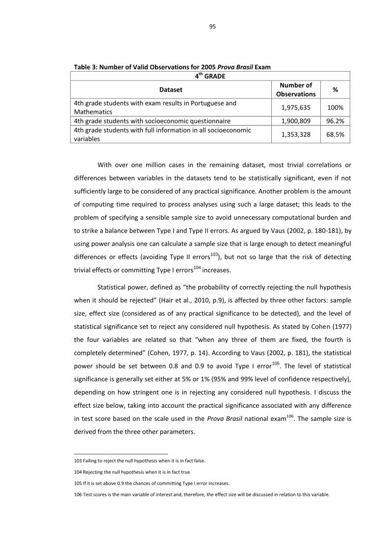
95
Table 3: Number of Valid Observations for 2005 Prova Brasil Exam
4th GRADE
Dataset Number of
Observations %
4th grade students with exam results in Portuguese and Mathematics
1,975,635 100%
4th grade students with socioeconomic questionnaire 1,900,809 96.2%
4th grade students with full information in all socioeconomic variables
1,353,328 68.5%
With over one million cases in the remaining dataset, most trivial correlations or
differences between variables in the datasets tend to be statistically significant, even if not
sufficiently large to be considered of any practical significance. Another problem is the amount
of computing time required to process analyses using such a large dataset; this leads to the
problem of specifying a sensible sample size to avoid unnecessary computational burden and
to strike a balance between Type I and Type II errors. As argued by Vaus (2002, p. 180-181), by
using power analysis one can calculate a sample size that is large enough to detect meaningful
differences or effects (avoiding Type II errors103), but not so large that the risk of detecting
trivial effects or committing Type I errors104 increases.
Statistical power, defined as “the probability of correctly rejecting the null hypothesis
when it should be rejected” (Hair et al., 2010, p.9), is affected by three other factors: sample
size, effect size (considered as of any practical significance to be detected), and the level of
statistical significance set to reject any considered null hypothesis. As stated by Cohen (1977)
the four variables are related so that “when any three of them are fixed, the fourth is
completely determined” (Cohen, 1977, p. 14). According to Vaus (2002, p. 181), the statistical
power should be set between 0.8 and 0.9 to avoid Type I error105. The level of statistical
significance is generally set either at 5% or 1% (95% and 99% level of confidence respectively),
depending on how stringent one is in rejecting any considered null hypothesis. I discuss the
effect size below, taking into account the practical significance associated with any difference
in test score based on the scale used in the Prova Brasil national exam106. The sample size is
derived from the three other parameters.
103 Failing to reject the null hypothesis when it is in fact false.
104 Rejecting the null hypothesis when it is in fact true
105 If it is set above 0.9 the chances of committing Type I error increases.
106 Test scores is the main variable of interest and, therefore, the effect size will be discussed in relation to this variable.

96
6.2.2 The Prova Brasil proficiency scale and how to gauge differences in test scores
(“effect size”)
Fourth grade test scores in Prova Brasil are expressed using a proficiency scale that
ranges from 125 to 325 points in Portuguese Language and from 125 to 350 points in
Mathematics. These represent the score intervals at which meaningful cognitive skills can be
identified and assessed amongst fourth and eighth grade examinees based on item response
theory107. A performance level is associated with each interval of the scale, based on a set of
cognitive skills characterising the expected learning achievements of students at that level.
Although the cognitive skills are different for each discipline and for each level of the scale,
results are comparable across grades and across time. Students who demonstrate skills at one
level also have the abilities represented in the lower levels of the scale. The Ministry of
Education does not set minimum performance levels to be achieved at the end of each grade
by discipline. The educational system is highly decentralised in Brazil, with the 27 states and
5,564 municipalities having autonomy in the organisation of the curriculum across grades and
the learning objectives for each grade. Hence, the national exam proficiency scale and test
score results are understood to be references based on which schools and school systems can
assess their educational objectives and, eventually, establish achievement goals for each
grade108.
In order to attribute practical significance to differences in test scores three alternative
measures are considered for each discipline: (i) an equivalent in amount of time of schooling
necessary to achieve a certain level of cognitive skills; (ii) an equivalent in percentage of the
interval between two adjacent cognitive levels (25 points); and (iii) an equivalent in standard
deviations observed in national exam results.
Using the scale range associated with meaningful cognitive skills for each discipline,
differences in mean test scores can be assessed considering an ideal mean number of points
per year necessary to achieve the top ranks of the scale (as shown in Table 4). On average, the
expected gains in cognitive skills for each year of schooling are equivalent to 25 points in
Portuguese Language and 28 points in Mathematics. This means that after four years of
regular schooling, a fourth grade student is expected to achieve 225 points in Portuguese
107 The same scale is used in the exam for the eighth grade, for which the top ranges of the scale are possibly achieved. However, as this research looks only at the effects on test scores at the fourth grade level, in general the highest scores are not expected to go beyond 300 points.
108 For instance, the State of São Paulo uses the same proficiency scale for the SARESP, the state level exam, in which students are classified into four different achievement levels (below basic, basic, adequate, and advanced) according to their scores.

97
Language109 and 237.5 points in Mathematics. By the end of the eighth grade, the student
would have achieved the upper bounds of the Mathematics and Portuguese scales110. By
considering the proficiency scale levels in such an ideal mode, fractions of one scale level can
be associated with months of schooling. For instance, one month of schooling equals 2.8
points in Portuguese Language and 3.1 points in Mathematics111. These figures can then be
taken as references for significant differences in assessing achievement gaps or potential
effects of BF on test scores, the expected effect size.
Table 4: Proficiency scale limits and average points per month to achieve the upper limit of the scale
Discipline Lower bound
Upper bound
Range Years of
schooling
Average points per
year
Average points
per month
Mathematics 125 350 225 8 28 3.1
Portuguese 125 325 200 8 25 2.8
An alternative criterion is to take the interval between two adjacent cognitive levels
and calculate differences in mean test scores as percentages of one cognitive level (as
described in Table 5). Associating the measured differences in test scores to percentages of
cognitive skills achieved by a student over one academic year creates practical meaning. For
instance, in Portuguese Language, an effect size of 2.5 points is associated with a 10%
difference in acquired cognitive skills, 5 points with 20%, 6.2 points with 25%, and so on.
Table 5: Points in test scores as percentages of one cognitive level in the proficiency scale
Discipline (%)
10% 20% 25% 50% 75% 100%
Mathematics 2.8 5.6 7 14 21 28
Portuguese 2.5 5 6.2 12.5 18.7 25
109 I consider here the progress achieved in four years in relation to the lower bound of the scale (125 points), for which meaningful learning was consistently measured.
110 This is a linear and, therefore, rather simplistic way of interpreting progress through the different cognitive levels of the proficiency scale. Nevertheless, the objective here is to offer a way of interpreting differences in test scores for which the approximation suffices.
111 I consider nine months of school attendance per year based on the mandatory minimum of 200 days per year in any grade of basic education.

98
A third possibility is to look at the distribution of test scores and to assess the practical
significance of observable differences as fractions of one s.d. Table 6 shows the main
descriptive statistics for test scores in Mathematics and Portuguese Language based on all
valid observations in the dataset for the fourth grade in 2005.
Table 6: Test Score in Mathematics and Portuguese – 4th grade 2005 – all valid observations
Discipline N mean s.d. p10 p25 p50 p75 p90
Mathematics 1,353,328 185.3 39.4 137.1 158.3 182.2 210.3 238.3
Portuguese 1,353,328 178.3 41.3 125.9 148.7 176.0 204.9 233.2
The test score distribution approximates to a normal distribution112. Sixty-eight
percent of students are found within one s.d. from the mean, approximately 95% lie within
two s.d., and 99.7% within three s.d. from the mean. One s.d. is approximately 40 points
measured on the proficiency scale for Mathematics and Portuguese Language. Differences in
test scores can be associated to fractions of one s.d., as shown in Table 7113. In this case,
differences as fractions of one s.d. can locate students at different points of the distribution.
For instance, a difference of 16 points in test scores between two groups of students
represents 0.4 of one s.d. This difference places the two groups at points of the distribution as
far as the median and the 65th percentile (182 and 198 points respectively114) in Mathematics.
Table 7: Points in test scores as fractions of one standard deviation in observable result for 2005
s.d. 0.1 0.2 0.3 0.4 0.5 … 1.0
Points 4 8 12 16 20 … 40
The three ways of interpreting points in the proficiency scale can be helpful in gauging
differences in test scores in terms of time of schooling, share of cognitive skills, or fractions of
an s.d. They also give us references to judge what a practically significant difference is when
assessing test scores using the proficiency scale, and I use them to interpret results in this
thesis. Any of the equivalent scales above can be used to calculate a reasonable sample size to
be used in the forthcoming analysis.
112 Skewness is 0.4 for both disciplines and kurtosis is 3.1 in Mathematics and 3.0 in Portuguese Language.
113 Once the standard deviation is very close for Portuguese and Maths I use an approximation of 40 points to calculate the
fractions in the table.
114 The 65th percentile of the distribution is 197.6 points on the scale.

99
6.2.3 Sample
The three different ways of attributing practical significance to differences in test
scores discussed above can give us an idea of the effect size one can expect to be meaningful
when assessing differences in means or coefficients in multiple regression analysis. For
instance, a test score value of 2.5 points represents 10% of one cognitive level in Portuguese
Language and can be used as a parameter to perform the statistical power analysis to calculate
the sample size necessary to achieve a balance between Type I and II errors. The null
hypothesis of zero test score difference between groups or zero effect on test scores of a given
variable can be tested against an alternative hypothesis of differences as small as 2.5 points by
randomly selecting at least 9,360 observations, as shown in Table 8115. This is the minimum
sample size required to detect an effect size that is equivalent to approximately 10% of one
cognitive level (or one month of schooling, or yet .06 of one s.d.) according to the conventional
use of α=.05 (statistical significance) and (1-β) = 0.8 (statistical power).
Table 8: Sample size and effect sizes (power=0.8 and alpha=.05)
Equivalence Effect Size Sample
Size
differing means 2.5 9360
regression slopes 2.5 9180
Note: two-sided test
A final remark on setting a sensible sample size is regarding the relative importance
given to the two possible errors in making statistical inferences. For example, by fixing power
at 0.8 and α=.05, we also set how we value the two possible errors. The probability ratio
between Type II error and Type I error is given by:
⁄
According to Cohen (1977, p.5), the ratio β/α provides the relative importance given to
each type of error by the researcher. In the case above, I implicitly consider the possibility of
committing Type I error to be four times more serious than making the Type II error, that is, I
consider the error of rejecting a true null hypothesis to be four times more important to avoid
than the error of failing to reject the null when it is actually false. This balance between Type I
and II errors pushes towards the necessity of stronger evidence to assert differences in test
scores between groups or significant effects on test scores.
115 The power analysis is performed using the software PS Power and Sample Size Calculations - Version 3.0, January 2009.
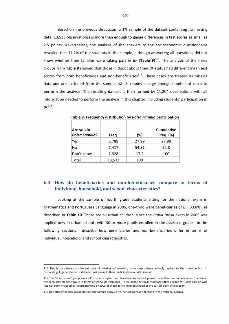
100
Based on the previous discussion, a 1% sample of the dataset containing no missing
data (13,533 observations) is more than enough to gauge differences in test scores as small as
2.5 points. Nevertheless, the analysis of the answers to the socioeconomic questionnaire
revealed that 17.2% of the students in the sample, although answering all questions, did not
know whether their families were taking part in BF (Table 9)116. The analysis of the three
groups from Table 9 showed that those in doubt about their BF status had different mean test
scores from both beneficiaries and non-beneficiaries117. These cases are treated as missing
data and are excluded from the sample, which retains a large enough number of cases to
perform the analysis. The resulting dataset is then formed by 11,204 observations with all
information needed to perform the analysis in this chapter, including students’ participation in
BF118.
Table 9: Frequency distribution by Bolsa Família participation
Are you in Bolsa Família? Freq. (%)
Cumulative Freq. (%)
Yes 3,788 27.99 27.99
No 7,417 54.81 82.8
Don’t know 2,328 17.2 100
Total 13,533 100
6.3 How do beneficiaries and non-beneficiaries compare in terms of
individual, household, and school characteristics?
Looking at the sample of fourth grade students sitting for the national exam in
Mathematics and Portuguese Language in 2005, one-third were beneficiaries of BF (33.8%), as
described in Table 10. These are all urban children, since the Prova Brasil exam in 2005 was
applied only in urban schools with 30 or more pupils enrolled in the assessed grades. In the
following sections I describe how beneficiaries and non-beneficiaries differ in terms of
individual, household, and school characteristics.
116 This is considered a different case of missing information, since respondents actually replied to the question but, in responding it, generated an indefinite position as to their participation in Bolsa Família.
117 The “don’t know” group scores 11.6 points higher than beneficiaries and 8.1 points lower than non-beneficiaries. Therefore, this is an intermediate group in terms of school performance. These might be those students either eligible for Bolsa Família who had not been included in the programme by 2005 or those in the neighbourhood of the cut-off point of eligibility.
118 One student is also excluded from the sample because his/her school was not found in the National Census.

101
Table 10: Bolsa Família participation (2005)
Are you in Bolsa Família?
Freq. %
No 7,416 66.2
Yes 3,788 33.8
Total 11,204 100.00
6.3.1 Student Characteristics
As shown in Table A - 1 there are remarkable differences between beneficiary and
non-beneficiary students in terms of demographic characteristics. The proportions of
beneficiary students in the North and especially in the Northeast, the poorest regions in Brazil,
are significantly higher than in the Centre-South regions. White students are significantly less
represented amongst beneficiaries compared to non-beneficiaries, whereas Afro-descendant
minorities, mixed-race groups, as well as indigenous groups and Asians are significantly more
represented amongst beneficiaries. Finally, looking at the distribution of students by age in the
two groups, those fourth graders at the right age-for-grade in 2005 (10 years old) appear in a
significantly higher proportion in the non-beneficiary group, whereas students aged 11 years
and older are proportionally more represented amongst beneficiaries. The proportion of boys
in the beneficiary group is slightly higher than that of girls.
The second set of characteristics displayed in Table A - 2 also shows significant
differences between beneficiaries and non-beneficiaries as to their school history. While 40%
of BF students have experienced at least one grade repetition over their years at school, the
proportion for non-beneficiaries is much lower (24%). The same is seen in the proportion of
those who have dropped out in past years. Roughly 10% of beneficiaries have abandoned
school in previous years, whereas this figure is lower amongst non-beneficiaries (around 7%).
Both retention and dropout are contributors to the overage indicator, which is 4.6 p.p. higher
for beneficiaries in the sample. Also, non-beneficiaries attended pre-school education in higher
proportions (79%) than beneficiaries (71%)119. Another important aspect distinguishing
students from both groups is the impressions of students regarding the attention they receive
in the classroom. Apparently, a much higher proportion of beneficiaries perceive themselves
to have been neglected in the classroom (22%) than do non-beneficiaries (14%). Also, there is
relatively less school mobility (ability to change schools) for beneficiaries compared to non-
beneficiaries (3 p.p.).
119 Although the proportion figures for those who declared to have attended pre-school are statistically equivalent, when taken together with the proportions of kindergarten attendance, the differences is 7 percentage points lower for beneficiaries.

102
The last set of variables in Table A - 3 accounts for students’ habits, reporting on
characteristics of students’ time allocation while not in school and their expectations as to
continuing in school. As the time spent watching television increases on the scale, the
difference in the proportions between the two groups increases in favour of non-beneficiaries.
This reveals that beneficiaries tend to spend fewer hours than non-beneficiaries watching
television. However, this result does not necessarily mean that beneficiaries are spending their
spare hours engaged in educational activities. In fact, as the differences in the next variable
show, beneficiaries spend more hours engaged in domestic work. In addition, the proportion
of beneficiaries in paid work is around 7 p.p. higher than that of non-beneficiaries. This could
also explain why beneficiaries are at a disadvantage when it comes to the share of students
who declare that they complete their homework120. The last variable in the table expresses
students’ expectations in relation to study and work after finishing compulsory education. The
majority of students in both groups expect to continue in school (≈ 60%) after completing their
fundamental education, either in combination with work or not. Nevertheless, many students
(≈30% in both groups) still did not know at that point (fourth grade) whether they would be
studying, working, or doing both in the future. Curiously, beneficiaries are slightly ahead in the
group declaring that they would be only studying in the future. This might express the
influence of BF on families and on children’s aspirations of continuing in school.
6.3.2 Household Characteristics
As expected, the material environment in beneficiary households is poorer when
compared to non-beneficiaries. As Table A - 4 shows, almost 10% of BF households do not
have running water and the proportion of those without power supply is almost double that of
their non-beneficiary counterparts (4% to 2%). In terms of durable goods, two patterns are
observed. Basic goods such as televisions, radios, and refrigerators are common even amongst
BF households (around 90% of respondents declare that they have these goods at home).
Differences between beneficiaries and non-beneficiaries range from 3 to 7 p.p. when
comparing those families without such goods. For goods such as VCRs, freezers, washing
machines, vacuum cleaners, and cars, the proportional difference between BF and non-BF
households for those not having such goods ranges from 7.5 to 16 p.p. With respect to housing
infrastructure, almost 4% of BF households do not have a bathroom and 1.5% of BF families
live in houses with no bedroom. These proportions are twice those of non-BF households.
120 The trends in the percentages are basically equal for Portuguese Language and Mathematics.

103
In terms of learning environment, Table A - 5 shows that non-BF households are at an
advantage compared to BF households. Approximately 60% of BF-households have less than
20 books; 13% do not even have a dictionary. Surprisingly, differences with non-BF households
are not substantial (4 and 3 p.p. respectively). More surprising is the fact that there is no
statistically significant difference between the two groups when asked if they have a peaceful
place to study at home. When it comes to computer and Internet access, the differences are
larger. Eighty-seven percent of BF households do not have a computer (against 75% of non-BF
households) and the proportion of non-BF households with Internet is double that of
beneficiary households.
Although BF households have a slightly higher proportion of female-headed families,
the two groups do not differ significantly in terms of parenting structure, as shown in Table A -
6. However, BF family sizes tend to be significantly larger, and the differences between the two
groups increase with the number of family members. BF beneficiaries are clearly at a
disadvantage where parental education is concerned. As described in Table A - 7, the BF group
has lower a proportion of mothers and fathers with secondary education or higher, whereas
the non-BF group has a lower proportion of parents with four years of education or less when
compared to the BF group. An interesting statistic is the 25% of students declaring that they do
not know their mothers’ level of education, and the 36% stating that they do not know their
fathers’ level of education. These proportions are statistically equivalent for beneficiaries and
non-beneficiaries. Beneficiaries also appear to be at a slight disadvantage (around 1 to 2 p.p.)
in relation to parental encouragement for students to pursue activities such as doing
homework, reading, going to school, and studying. BF parents are also less engaged in
attending school meetings.
The material disadvantages of BF-households are expected, given that the programme
is designed to target the poorest families. Nevertheless, the disadvantages of BF students at
home go beyond their material environments, and include family structure, parents’
characteristics, and level of parental encouragement. The question of whether the material
and learning environment is more influential on children’s outcomes than family structure and
parents’ characteristics is analysed later in this chapter.
6.3.3 School Characteristics
School infrastructure is assessed in terms of school size, facilities, and available
equipment. School facilities are measured by an index ranging from zero to one, computed

104
using binary variables for 34 items included in the National School Census in 2005121. School
libraries, computer rooms, and laboratories are also examined separately from the general
facilities index, because they represent resources directly linked to pedagogical purposes. A
second index for school equipment, ranging from zero to one, measures the availability of 19
items included in the School Census122. Two variables related to school organisation measuring
student-teacher ratio and class size are compared for the two groups. The former is a proxy for
the intensity of teacher interaction with students. For instance, in many primary schools in
Brazil the four basic areas of study123 for grades 1 to 4 are divided between two (sometimes
amongst four) teachers. Also, some school projects include special teachers for library,
computer, physical education, and arts activities, decreasing that ratio and enabling students
to have more options for teachers to support them. These two variables are measured for
grades 1 to 4 altogether, since they are not disaggregated by grade in the available data. The
student-teacher ratio is correlated with class size124, although the two indicators measure
different aspects of school organisation. Finally, teachers’ characteristics are described in
terms of teachers’ education and in relation to class management by discriminating between
those who assign homework to students on a regular basis and those who regularly correct the
homework.
School resources differ significantly for beneficiaries and non-beneficiaries. As
displayed in Table A - 8, beneficiaries tend to attend smaller schools on average, which could
explain why they also attend schools with fewer resources when it comes to school facilities.
Beneficiaries are found in higher proportions in schools without libraries or reading rooms,
computer rooms, or laboratories. Also, for the two calculated indexes (facilities and
equipment), differences, however small, are in favour of non-beneficiaries. Student-teacher
ratio and class size do not differ significantly between the two groups and have lower
statistical significance (Table A - 9). Although beneficiaries tend to attend schools with a
slightly higher student-teacher ratio, the available data reveals a trend in favour of BF students
in relation to class size. However, the difference in teachers’ education is substantial between
the two groups. There is a 7 p.p. difference in the proportion of teachers with higher
education, with beneficiaries attending schools where teachers tend to be less qualified (as
121 The facilities include administrative rooms, resource rooms, sport areas, infant education spaces, sanitation facilities, alimentation areas, special education resource rooms, laboratories, and meeting rooms. The index is calculated by dividing the number of facilities in the school by the total number of facilities assessed in the National School Census.
122 The category includes devices such as audio-video equipment, photocopy machines and printers, overhead and PowerPoint projectors.
123 Mathematics, Portuguese Language, Social Studies, and Sciences.
124 The correlation coefficient is 0.54.

105
shown in Table A - 10). Also, beneficiaries are more represented in schools where teachers do
not tend to correct the homework for both disciplines (around 3 p.p. difference). However, no
significant differences are found between beneficiaries and non-beneficiaries regarding
teachers who do not assign homework. School characteristics do not favour the already
disadvantaged BF group. On the contrary, instead of compensating for family background by
supplying an improved school environment, education systems seem to reinforce inequalities
between the two groups, as beneficiaries attend schools that are less well-resourced than
those attended by non-beneficiaries.
At this point is important to highlight that all of the differences presented between
beneficiaries and non-beneficiaries may, in fact, be downgraded, since by October 2005 not all
eligible families were registered in the programme125 (MDS, 2005). It is likely that there are
children amongst the non-beneficiaries for which the observed characteristics are likely to be
very similar to those of beneficiaries. If this is true, the differences between the two groups are
underestimated. In addition, as mentioned, Prova Brasil is only applied in urban schools; 23%
of BF beneficiaries are enrolled in rural schools126 that are not surveyed, probably further
reducing the estimated differences between the two groups.
In sum, looking at how the two groups are distributed in relation to individual,
household, and school characteristics it can be seen that, on average, BF students are not only
socially disadvantaged (as expected for those eligible for the programme). They are also in a
situation of educational disadvantage, entrenched in their personal school histories and in the
schools they attend, which are, in many respects, less well-resourced than the schools
attended by non-beneficiaries. As a result, the educational gap extends to school outcomes,
measured by performance in test scores, as shown in the next section.
6.4 The achievement gap between beneficiaries and non-beneficiaries
I now look at the characteristics of the test score distribution, how test scores differ
between beneficiaries and non-beneficiaries, and how the mean test score varies according to
specific students’ socioeconomic and school characteristics available in the dataset. The
characteristics described in the previous section distinguish students and their performance on
the exam. These characteristics also partially explain the existing achievement gap between
beneficiaries and non-beneficiaries, and this section will also identify which of those amongst
125 According to the Ministry of Social Development, in October 2005 there were 8 million families already registered in Bolsa Família out of an estimated 11.2 million eligible families.
126 This figure is based on available data from 2007 for all beneficiary children.

106
them are the most relevant. Inasmuch as BF can influence some of these factors, it can
potentially contribute to reducing the achievement gap.
6.4.1 Test scores distribution and association with income
Table 11 shows the main statistics for the fourth grade test score distribution
considering the sample taken from the 2005 Prova Brasil national dataset.
Table 11: Test Score in Mathematics and Portuguese – 4th Grade/ 2005 Variable N mean s.d. p10 p25 p50 p75 p90 skewness kurtosis
Mathematics 11,204 186.1 39.9 136.6 158.4 183.2 212.3 240.0 0.3 3.0 Portuguese 11,204 179.0 42.1 125.5 148.2 176.9 206.2 234.9 0.3 2.9
Based on the values for skewness and kurtosis127 as well as on the shape of the
distributions depicted in Graph 10 and Graph 11, it can be concluded that the test score
distribution for both disciplines assumes, with good approximation, the symmetrical
characteristic of a normal distribution. Based on this approximation and the properties of the
normal distribution, inferences can be made about the population parameters using estimated
parameters from the sample.
Graph 10: Test Score Distribution – Mathematics 4th grade
127 Skewness and kurtosis statistics for a normal distribution are 0 and 3 respectively.
0
.002
.004
.006
.008
.01
Den
sity
100 150 200 250 300 350Test Scores
Prova Brasil 2005: 4th grade - Maths
Histogram

107
Graph 11: Test Score Distribution – Portuguese 4th grade
Fourth grade test scores in Portuguese Language and Mathematics for beneficiaries
and non-beneficiaries are reported in Table 12. On average, BF beneficiaries perform less well
than non-beneficiaries and below the national mean in both disciplines. The dispersion of
results amongst beneficiaries is slightly smaller than for non-beneficiaries. The distributions for
both disciplines by group are shown in Graph 12 and Graph 13.
Table 12: Average 4th grade test scores in Mathematics and Portuguese by participation in Bolsa Família
4th Grade Test Scores
Are you in Bolsa Família?
No Yes
N Mean s.d. Min. Max. N Mean s.d. Min. Max.
Mathematics 7416 191.6 40.5 79.1 330.6 3788 175.4 36.5 84.10 330.41
Portuguese 7416 185.7 42.7 75.7 321.0 3788 166.0 37.6 81.0 321.2
Graph 12: Mathematics test score distribution by BF participation
0
.002
.004
.006
.008
.01
Den
sity
50 100 150 200 250 300
Test Scores
Prova Brasil 2005: 4th grade - Portuguese
Histogram
Mean=191.6
Mean = 175.4
0
.005
.01
.015
0
.005
.01
.015
100 200 300 400
No
Yes
Den
sity
Test Scores - MATHS - 4th gradeProva Brasil 2005
Are you in Bolsa Familia?

108
Graph 13: Portuguese test score distribution by BF participation
Table A - 11 and Table A - 12 report the statistical tests for equality of mean test
scores in Mathematics and Portuguese for the two sub-groups in the sample (beneficiaries and
non-beneficiaries of BF). The respective differences ∆=16.2 and ∆=19.7 between the two
groups are statistically significant and are equivalent to 65% and 77% of one cognitive level in
the Prova Brasil proficiency scale. This means that, on average, beneficiaries are lagging behind
by approximately two-thirds of one cognitive level in Mathematics and by three-quarters in
Portuguese. Those differences correspond to approximately 0.4 and 0.5 s.d. from the national
mean. The differences can also be translated into five and seven months of schooling
respectively. Thus, we can see that although the two groups do not differ substantially in terms
of the observed variance in each discipline, they do differ as to the mean achievement in test
scores in both subjects, both in statistical terms and in practical significance. Why should this
be the case? What can explain the gap?
Beneficiaries perform less well than non-beneficiaries on average. They come from the
poorest households in the sample according to BF eligibility rules and they tend also to be
disadvantaged in many respects that can negatively influence their performance at school.
These disadvantages include the material conditions and learning environment at home, and
family structure or parents’ characteristics (including level of education, support, and
encouragement for children’s education). As stated by Jencks in his classic book, Inequality,
“the way a family brings up its children is obviously influenced by its economic position”
(Jencks, 1972, p.78). The association between a family’s income level and children’s school
outcomes has long been reported in the literature (as discussed in chapter two), despite the
controversial debate on the extent of such influence and whether it is a causal relationship.
Mean = 185.7
Mean = 166.0
0
.005
.01
0
.005
.01
100 200 300
No
Yes
Den
sity
Test Scores - Portuguese - 4th grade
Are you in Bolsa Família?
Prova Brasil 2005

109
Using Prova Brasil 2005 data, that association can also be found in the case of Brazilian
children.
Because the socioeconomic variables available in Prova Brasil 2005 do not include
household income, I use a proxy to estimate the mean household income and then look at the
association with the mean test score. The proxy variable measures the number of durable
goods in the household (household goods index)128. In examining the test score mean values
by that proxy, a clear association
between the mean test scores in both
disciplines and the durable goods index
can be observed, as shown in Graph 14.
The dotted lines represent the mean test
score value for the entire sample of
fourth grade students in Mathematics
and Portuguese Language. Across the
range of values for durable goods, the
mean test score in Mathematics is higher
than in Portuguese. Assuming that the
index for durable goods indirectly
indicates the expected socioeconomic
status in terms of the mean household per capita income, it can be argued that, on average,
the higher the household income per capita the higher the child’s school outcomes as
measured by test scores. That, in principle, could explain the differences in test scores
between beneficiaries and non-beneficiaries. To see whether that is the case, I look at the
same association shown in Graph 14 for beneficiaries and non-beneficiaries when analysed
separately.
As shown in Graph 15 and Graph 16, the mean test score for beneficiaries follows a
different pattern. While the mean test score in both disciplines for non-beneficiaries
continuously increases with the proxy for the mean household income per capita, the mean
test scores for BF children do not present the same trend over the goods index. The test score
128 The validity of this variable as a proxy for the mean household income per capita is tested using 2005 data from the National Household Sample Survey (PNAD) for a subset of the same durable goods surveyed in the Prova Brasil socioeconomic questionnaire in 2005 (radios, televisions, washing machines, refrigerators, freezers, and computers). The A- Graph 1 in the appendix presents this association. This proxy is used here only to illustrate the association between family income and students’ achievement in test scores. This is a very inefficient estimator of the household per capita income, as can be seen by the size of the standard deviation and the loss of accuracy as we move upwards in the goods index scale presented in Table A - 13. This means that a very poor family can also have a high goods index, although the association with the mean household income per capita is valid on average for the entire rank of goods index.
Graph 14: Mean test scores by household goods index

110
gap between the two groups does not exist for the first range of the goods index values (up to
0.3 in Mathematics and 0.2 in Portuguese). That could be explained by the fact that non-
beneficiaries at those associated levels of income probably have family situations that are
more similar to those eligible to take part in BF than to their non-beneficiary counterparts,
although they were not yet registered in 2005129. The two groups then detach from each other
and the gap in terms of mean test scores increases across the levels of the goods index. Why
does this happen? Why does the beneficiary group’s mean not follow a clear increasing
pattern (tending to decrease across the upper ranks of the goods index)?
An evident explanation is that the durable goods index, as a proxy for household per
capita income, does not account for the variance in this variable, and it also loses accuracy as
we move upwards on the scale as made clear by the increasing s.d. presented in Table A - 13.
This means that a very poor family can also have a high goods index in the sample. Although
the association between mean test scores and mean household income per capita (as
measured by the goods index) is valid, on average, for the entire rank of goods index in the
population, the goods index is an inaccurate proxy for the average income for the beneficiary
group. This group is located at the lower extreme of the income distribution in each level of
the goods index. In fact, since the threshold for a family to take part in the programme in 2005
was R$ 100130 (approximately US$ 45) per capita, we can assume that for the beneficiary group
the income level is actually constrained throughout the ranks of the goods index, while that
“ceiling” does not apply for non-beneficiaries. In that sense, the trend lines in Graph 15 and 129 As explained earlier, by 2005 the number of poor families registered in the programme was around 8 million out of 11.2 million estimated poor families.
130 This threshold was established by the Presidential Decree No 5.209, 17 September 2004, for families with school-age children. For families in extreme poverty without children, the threshold was 50 reais per capita (approximately US$ 23 in 2005).
Graph 15: Mean test scores (Maths) by household goods index and participation in Bolsa Família
Graph 16: Mean test scores (Port.) by household goods index and participation in Bolsa Família

111
Graph 16 are, in fact, representing the achievement gap in test scores between the two groups
at different levels of non-beneficiaries’ income, since the mean household income per capita
for the non-beneficiary group increases while the beneficiaries’ mean household income is
roughly within the same band. Therefore, on average, the achievement gap between
beneficiaries and non-beneficiaries increases with the increasing gap in the household per
capita income.
Nevertheless, there are important factors other than income intervening in children’s
outcomes that also characterise the condition of deprivation, and that might contribute to the
gap between those groups across income levels. For instance, as previously described in this
chapter, beneficiaries attend schools where teachers tend to be less qualified. If teachers’ pre-
service education is positively correlated with students’ test scores, then the negative
difference in test scores for beneficiaries could be explained, at least partially, by the fact that
they are attending schools with less qualified teachers. It might be the case that the difference
in test scores between the two groups is due also to the fact that beneficiaries tend to be in
the labour force in higher proportions than non-beneficiaries. This would make the time
allocated to school activities, including homework and study at home, more restricted for
beneficiaries. Parents’ characteristics could also have an influence in producing that difference,
since beneficiaries’ parents tend to be less educated on average than the parents of non-
beneficiaries. If parents with more education tend to be more effective in supporting children
in school activities at home, the difference in test scores could be due to the education gap
between the parents of the two groups. Controlling for variables such as these will give us a
better understanding of at least some of the factors other than income explaining that
difference.
6.4.2 How do test scores vary according to Bolsa Família participation taking into
account specific characteristics of students, families, and schools?
One way to condition out possible influences on the mean test score difference
between beneficiaries and non-beneficiaries is to estimate the coefficient associated with the
indicator of programme participation while controlling for other possible factors in a
regression function, as described below. Using multiple regression analysis, this section
explores how test scores vary according to different factors related to students’ social
background and school environment, particularly family participation in BF. Different models
are created by introducing additional explanatory variables in an attempt to assess their
influence on the observed gap between beneficiaries and non-beneficiaries. By adding sets of

112
variables in the successive models, I examine how their inclusion interferes with the size and
direction of the estimated coefficients already in the model, especially the parameter α
associated with the variable indicating BF participation. The general model to be estimated is
represented below, whose variables are described in the following paragraphs.
Model 1
∑
In Model 1 the variable yi represents the test score for the student i; Xki represents the
observed characteristic k for the student i; BFi is a dummy variable expressing whether the
student’s family takes part in BF; and ui is the error term expressing all other factors affecting
test scores that are not included in the model. The factors (Xki), to be introduced in the model,
are those describing student, household, and school characteristics.
Since all available variables in the 2005 Prova Brasil socioeconomic questionnaire are
categorical, in some cases containing several levels, I reduced the number of categories
whenever convenient for the sake of simplification and parsimony. This is done by collapsing
variable levels based on the substantial similarity of the categories involved and also on the
differences observed in test scores between the categories. For instance, taking the students’
school history variables and plotting the mean test score in Portuguese Language for each
category against the overall mean (Graph 17) we observe that all the variables in the set can
be collapsed into binary values.
No
Many times
Some times
No
Yes, twice >Yes, once
Yes, twice >
No
Yes, once
No, private
Yes
No, public
Kindergarden
Pre-school
1st grade
Yes
No
15
016
017
018
019
0
Mea
n te
st score
Overage Start Grade Never changed school Failure Dropout Neglected
4th grade - Portuguese
Mean Test Score by Student School History
Graph 17: Mean Test Score by Student School History

113
Some of the categories are clustered on one side of the red line, which represents the
mean test score considering all students in the sample (179 points). For instance, the overage
variable is already a binary variable131, but the entrance grade variable can also be collapsed
into two categories: those students entering at any pre-school132 level and those starting in the
first grade. School swap can also be collapsed into those who have changed schools and those
who did not change schools before fourth grade. Failure at any grade during the first four
years of schooling can be reduced to two categories: those who failed and those who did not
fail; the same is applied to dropouts. Finally, the impression of being neglected in the
classroom can be also converted into a binary variable by collapsing those declaring to have
felt neglected many times or sometimes, so forming a common category of students who
experienced isolation in school, against those declaring not to have had such an experience.
The same logic is applied to all the other categorical variables used in the regression analysis
(except region)133. The mean test score in Portuguese Language, plotted by the remaining
categorical variables, is displayed in A- Graph 2 to A- Graph 7 in the appendix; and the
resulting sets of variables used in the regression analysis are described in Table 13134.
131 It is constructed by considering students who are two years or more above the recommended age (10 years old) for the fourth grade as overage students.
132 At the time the questionnaire was created, pre-school in Brazil was formally understood to be for children ages of 4 to 6 years old (a non-compulsory level of education) and was informally grouped into “maternal” education (for 4 year-olds), “jardim de infância” (for 5 year-olds), and “pré-escola” (sometimes meaning any of the previous and/or for 6 year-olds). As the questionnaire uses three categories, I translate them here as follows: “jardim de infância / maternal” is designated as “kindergarten”; “pré-escola” is designated as “pre-school”, and “primeira série” is designated as the first grade. The first two categories are collapsed into “pre-school” in line with the official definition.
133 In the case of the variables indicating durable goods, they are used to create a new variable (durable goods index) ranging from zero to one.
134 Table A - 14 to Table A - 16 in the appendix show the statistical difference between beneficiaries and non-beneficiaries with respect to these variables.

114
Table 13: Description of variables used to estimate Model 1
VARIABLES DESCRIPTION D
emo
grap
hic
C
har
acte
rist
ics
Bolsa Família Dummy variable equal to 1 if the pupil is BF beneficiary.
Male Dummy variable equal to 1 if the pupil is male.
Non-white Dummy variable equal to 1 if the pupil is non-white.
Sch
oo
l H
isto
ry
Overage Dummy variable equal to 1 if the pupil is two years or more above the recommended age for the 4
th grade (10 years-old)
Pre-school Dummy variable equal to 1 if the pupil started school before the 1st
grade.
Same school Dummy variable equal to 1 if the pupil has not changed school since the 1
st grade.
Fail Dummy variable equal to 1 if the pupil has failed any grade in past years.
Dropout Dummy variable equal to 1 if the pupil has dropped out any time in past years
without returning until the end of the academic year.
Neglected Dummy variable equal to 1 if the pupil declares feeling neglected in the classroom.
Hab
its
and
Ex
pec
tati
on
s
Watch-TV Dummy variable equal to 1 if the pupil declares watching TV at home.
Domestic work (2h or more)
Dummy variable equal to 1 if the pupil declares working at home for two or more hours a day.
Child Labour Dummy variable equal to 1 if the pupil declares being engaged in any form of work outside home.
Do Homework Port. Dummy variable equal to 1 if the pupil declares doing Portuguese Language homework at least once in a while.
Do Homework Maths Dummy variable equal to 1 if the pupil declares doing Mathematics homework at least once in a while.
Intend to continue studies
Dummy variable equal to 1 if the pupil declares intention to continue studies after concluding compulsory education.
Mat
eria
l En
viro
nm
ent
Electricity Dummy variable equal to 1 if the pupil declares living in a house with power supply.
Tap Water Dummy variable equal to 1 if the pupil declares living in a house supplied with piped water.
Bedroom Dummy variable equal to 1 if the pupil declares living in a house with at least one
bedroom.
Bathroom Dummy variable equal to 1 if the pupil declares living in a house with at least one bathroom.
Dictionary Dummy variable equal to 1 if the pupil declares living in a house with at least one dictionary.
Peaceful place to study
Dummy variable equal to 1 if the pupil declares having a peaceful place to study at home.

115
VARIABLES DESCRIPTION
Books ≥ 20 Dummy variable equal to 1 if the pupil declares living in a house where there are 20 or more books.
Computer Dummy variable equal to 1 if the pupil declares living in a house with a computer (with or without internet).
Goods (0-10) Number of durable goods at pupil’s home measured amongst 10 items surveyed in the socioeconomic questionnaire.
Fam
ily
Stru
ctu
re Family size (≥ 7) Dummy variable equal to 1 if the pupil declares living in a house with 7 or more
people. Both parents Dummy variable equal to 1 if the pupil declares living with both parents.
Par
ents
’ C
har
acte
rist
ics
Mother Educ. (post-primary)
Dummy variable equal to 1 if the pupil declares the mother has completed secondary school or College.
Father Educ. (post-primary)
Dummy variable equal to 1 if the pupil declares the father has completed secondary school or College
Parents in school meetings
Dummy variable equal to 1 if the pupil declares parents often attend school meetings.
Parents encouragement (0-4)
Index number ranging from 1 to 4 measuring parents incentives to pupil’s education. The four binary components are: incentive to study, incentive to do homework, incentive to read and incentive to go to school.
Sch
oo
l In
fra-
Stru
ctu
re Facilities (0.0 - 1.0) Index number ranging from 0 to 1 measuring the availability of school facilities
amongst 34 items measured by the National School Census in the school attended by the pupil.
Equipment (0.0 – 1.0) Index number ranging from 0 to 1 measuring the availability of school equipment amongst 19 items measured by the National School Census in the school attended by the pupil.
Teac
her
s
Student/teacher ratio Number of pupils enrolled in grades 1 to 4 divided by the number of teachers working in grades 1 to 4 in the school attended by the pupil.
Prop. teachers HE Proportion of teachers with higher education working in grades 1 to 4 in the school attended by the pupil.
Teacher correct homework (Port.)
Dummy variable equal to 1 if the pupil declares teacher often corrects Portuguese Language homework.
Reg
ion
North Dummy variable equal to 1 if the pupil’s school is located in the North region.
Northeast Dummy variable equal to 1 if the pupil’s school is located in the Northeast region
Central-West Dummy variable equal to 1 if the pupil’s school is located in the Central-West region
South Dummy variable equal to 1 if the pupil’s school is located in the South region

116
(1) Student Characteristics and Test Scores
The regression analysis is carried out using test scores in Portuguese Language as the
dependent variable. Table 14 reports the regression coefficients and robust standard errors for
the three models encompassing students’ characteristics and how the coefficient for BF
participation changes across these models.
Table 14: Regression of Portuguese Test Score on STUDENT CHARACTERISTICS – 4th grade (1) (2) (3) (4) VARIABLES Portuguese Portuguese Portuguese Portuguese
Bolsa Família -19.7*** -18.5*** -14.1*** -13.0*** (0.787) (0.784) (0.761) (0.752)
Male -7.8*** -5.7*** -4.8*** Demographic (0.768) (0.736) (0.738) Characteristics Non-white -9.5*** -6.3*** -6.0*** (0.809) (0.771) (0.757)
Overage -7.4*** -4.7*** (1.266) (1.261) Pre-school 11.9*** 10.8*** (0.831) (0.823) Student’s Same school -0.5 -0.3 School History (0.745) (0.733) Fail -17.3*** -16.2*** (0.827) (0.816) Drop -7.1*** -4.7*** (1.335) (1.321) Neglected -10.4*** -9.1*** (0.733) (0.724)
Watch TV 6.2*** (0.990) Domestic Work (2h or more) -9.1*** (0.965) Child labour -13.3*** (1.003) Student’s Do Homework Port. 10.0*** Habits and Expectations
(1.415)
Do Homework Maths 3.4* (1.813) Intend to continue studies 3.6*** (0.735)
Constant 185.7*** 195.1*** 193.1*** 174.8*** (0.496) (0.778) (1.153) (2.380) Observations 11,204 11,204 11,204 11,204 R-squared 0.049 0.070 0.162 0.191
Robust standard errors in parentheses *** p<0.01, ** p<0.05, * p<0.1
Student characteristics alone explain 19% of the variance in test scores and reduce the
gap between beneficiaries and non-beneficiaries by around 34% (from -19.7 to -13.0 points).
Several factors stand out as contributors to students’ performance in test scores. Male and
non-white students are at a disadvantage in the Portuguese exam, regardless of their status as
117
beneficiaries or non-beneficiaries. Other factors related to students’ school histories, habits,
and expectations reveal potential influences on their performance.
School history has strong explanatory power with respect to test scores, since its
inclusion more than doubles the explained variance, as seen in the R2 reported in model (3).
Three factors stand out: (i) early childhood education, as measured by pre-school
participation; (ii) the experience of failing; and (iii) the experience of being neglected in the
classroom. First, pre-school attendance holds a significant and positive coefficient in the
regression model on test scores achievement, estimating approximately 0.2 to 0.3 s.d. increase
on average. In the literature, early childhood education is strongly supported as a major
contributor to students’ future performance at higher grades in their school life (Leuven and
Oosterbeek, 2007; Esping-Andersen, 2009, p. 132-7). Pre-school not only prepares children for
primary school, but, in general, also means better nutritional care in childhood for the poorest
children. It can also bridge the transition between home and school for the youngest, giving
them more self-confidence and precocious stimulus for school activities. Amongst BF
beneficiaries, those who attended pre-school are less likely to have dropped out or failed
during the first four years of primary school135.
Second, by failing a grade during the early school years a child can see his/her results
in Portuguese at the fourth grade reduced by approximately 0.4 s.d. according to model (4). By
driving a child to repeat a grade the school system is probably inflicting a deleterious effect on
her/his self-esteem, causing more harm than benefit in the school years to come. There are no
learning gains in repeating a grade; on the contrary, on average repeaters perform less well
following this experience. It is also worth noting that when the variable for grade failure is
included in the model, the overage coefficient loses statistical significance after all controls are
considered (see Table A - 17). This is not surprising, since failing a grade is an obvious cause of
being overage136 in subsequent grades. ‘Overage’ is a cumulative or stock variable recording
students’ previous school histories. Either by failing and consequently repeating a grade, or by
dropping out and returning to the same grade in the following year, the pupil enters the
overage group and increases the school age-grade distortion.
135 Amongst beneficiaries, 36% of those who attended pre-school failed a grade over their first four years of primary education, against 49% of those who did not attend pre-school. For non-beneficiaries, the figures are 21% and 38% respectively. For both groups, early childhood education is positively associated with fewer chances of failing a grade.
136 The overage variable indicates those pupils two years or more above the recommended age for the fourth grade (10 years-old). Overage has been reported in the literature as a relevant factor associated with students’ school achievement. In general, students who experienced multiple repetitions and/or late entrance to school end up composing a group ahead of the recommend age for grade. They also perform worse in school, on average.

118
Third, being ignored in the classroom has a significant negative effect on test scores, as
estimated in the model, and is a subjective element concerning students’ perceptions of
teachers’ attitudes towards them137. The feeling of being neglected or dispensed insufficient
attention in the classroom can negatively affect students’ self-esteem and can also contribute
to their isolation and loss of interest in school matters. On average, the lack of attention and
support from teachers felt by students is roughly associated with a 0.2 s.d. decline on test
scores.
The second set of individual characteristics analysed is students’ habits and
expectations about their future schooling. Three major factors stand out: (i) home chores; (ii)
child labour; and (iii) homework. First, a significant negative effect on students’ performance is
captured by the variable indicating home chores done by children for two hours or more on a
daily basis. By allocating time to domestic work, children lose around 0.2 s.d. on average in
their performance. Second, and in the same direction, being involved in any form of child
labour138 negatively impacts students’ performances, and is the second largest effect amongst
all the variables (0.3 s.d.). These two variables have independent effects on test scores. Third,
students’ habits of doing homework (in this case, Portuguese Language homework) have a
significant positive effect on test scores (0.2 s.d.). Whether the student does mathematics
homework has no effect on Portuguese test scores, but having expectations of carrying on
studies after completing fundamental education is positively correlated with test scores.
(2) Household Characteristics and Test Scores
Household factors, when taken alone, explain 14% of the variance in test scores and
also explain some of the differences in test scores between beneficiaries and non-
beneficiaries, as shown in Table 15 (a reduction of 26% from -19.7 to -14.6).
137 The dummy variable captures those students stating different levels of experience in feeling ignored in the classroom, ranging from “many times” to “once in a while”, against not having or rarely having such a feeling.
138 Child labour here refers to any form of outside home work in which children allocate time.

119
Table 15: Regression of Portuguese Test Score on HOUSEHOLD CHARACTERISTICS – 4th grade (1) (2) (3) (4) VARIABLES Port_4th Port_4th Port_4th Port_4th
Bolsa Família -19.7*** -16.7*** -15.8*** -14.6*** (0.787) (0.792) (0.791) (0.785)
Electricity 17.4*** 16.2*** 13.2*** (2.233) (2.220) (2.196) Tap Water 11.3*** 10.6*** 9.0*** (1.319) (1.304) (1.293) Bedroom 12.9*** 12.3*** 10.7*** (3.846) (3.748) (3.648) Material Bathroom 11.7*** 11.4*** 10.4*** Environment (2.191) (2.177) (2.118)
Dictionary 9.5*** 9.4*** 7.2*** (1.214) (1.202) (1.189) Peaceful place to study 5.4*** 4.5*** 1.9* (1.066) (1.062) (1.057) Books ≥ 20 -3.4*** -2.6*** -3.8*** (0.855) (0.852) (0.838) Computer 3.7*** 3.7*** 1.3 (1.188) (1.177) (1.174)
Goods (0 - 10) 1.7*** 1.4*** 0.7*** (0.245) (0.244) (0.243)
Family size (≥ 7) -10.5*** -9.5*** Family (0.863) (0.856) Structure Both parents 4.4*** 3.8*** (0.809) (0.801)
Mother Educ. (post-primary) 8.4*** (1.058) Father Educ. (post-primary) 3.2*** Parents’ (1.048) Characteristics Parents in school meetings 8.0*** (0.756) Parents encouragement (0-
4) 5.8***
(0.491)
Constant 185.7*** 111.7*** 115.7*** 101.7*** (0.496) (4.628) (4.565) (4.602) Observations 11,204 11,204 11,204 11,204 R-squared 0.049 0.093 0.106 0.137
Robust standard errors in parentheses *** p<0.01, ** p<0.05, * p<0.1
Factors related to the household’s material environment, although explaining only a
minor part of the variance in test scores, are very good discriminators of the poorest families.
Households with no bathroom or no bedroom, or as yet deprived of power and water supplies
are probably amongst the poorest in the country. Children from families living in such
environments are at a significant disadvantage, as can be seen by the associated coefficients
shown in Table 15. Looking at material factors related to what I call the “learning environment
at home” (dictionaries, books, computers, and a peaceful place to study) the dummy variable
for dictionary is the only one to keep its significance, even when all other controls are included
120
in the regression (Table A - 17)139. The amount of durable goods does not hold any practical
significance for test scores in the context of the other household characteristics.
Family structure (size and having both parents) is also influential on test scores. Larger
families in deprived contexts generally face more hardships, but can also provide extra hands
to work as breadwinners. Large families in the examined sample are associated with the
presence of child labour140 and can suggest less time allocated per child when education
support at home is considered. This is reflected in the negative coefficient associated with
families with seven or more members living in the same household (a reduction of 0.2 s.d.).
Results also show an advantage for children living with both mother and father, as opposed to
those living with a lone parent or with no parents at all. This can reflect the household’s
income, but also more support from parents and a more stable environment for children.
Looking at the disaggregated data, lone parenting has a negative association with children’s
performance (with lone fathers as the worst).
Parents’ characteristics, particularly the mother’s education, are positively associated
with children’s performances on test scores. This can reflect two different circumstances.
Mothers can be more present in children’s day-to-day life, even when at work or raising
children on their own; they can also play the main role as caregivers in the family, while
fathers are the main breadwinners. It is worth noting that children whose parents hold a
secondary school degree are at more of an advantage in relation to children whose parents
have less than four years of education, than children whose parents hold a degree in higher
education. Other results can help to understand this trend. A higher proportion of parents with
secondary education attend school meetings (66%)141 and they also have a higher mean in the
index for parents’ encouragement for children’s education (3.78). A possible explanation is
that parents’ who achieved secondary education are keener to make an extra effort so that
their children can achieve higher levels of education. Parents’ encouragement for children’s
education and attendance at school meetings are also significantly correlated with test scores.
Nevertheless, the relationship between parents’ attendance in school meetings and test scores
could actually be working in the opposite direction. Parents whose children perform better at
school end up feeling proud of them and they are willing to go to school to hear compliments
from teachers, whereas parents whose children are performing poorly or are known by their
139 In this case, having a computer becomes statistically significant.
140 Cross-tabulation between child labour and family size shows that the larger the family size, the higher the proportion of children engaged in child labour.
141 The percentage for higher education holders is 64%, for fundamental education (eighth grade) holders it is 59%, and for those with fourth grade or less it is 57%.

121
bad behaviour at school may feel embarrassed or be unwilling to attend school meetings. Both
factors remain significant, even after controlling for all variables in the full model (Table A - 17)
representing a 0.1 s.d. increment for test scores.
(3) School Characteristics and Test Scores
The regression of Portuguese Language test scores on school factors is reported in
Table 16. The output shows that school factors not only explain the smallest share of the
variance in test scores so far (around 10%), but is also the set of factors that has the smallest
effect in reducing the observed gap between beneficiaries and non-beneficiaries in test scores
(from -19.7 to -16.8, around a 15% reduction).
Table 16: Regression of Portuguese Test Score on SCHOOL CHARACTERISTICS – 4th grade (1) (2) (3) (4) Beta for VARIABLES Portuguese Portuguese Portuguese Portuguese Model (4)
Bolsa Família -19.7*** -17.3*** -17.3*** -16.8*** -0.189 (0.787) (0.784) (0.783) (0.778)
Facilities (0.0 - 1.0) 29.1*** 27.2*** 21.9*** 0.056 Infrastructure (4.100) (4.110) (4.144) Equipment (0.0 – 1.0) 36.7*** 35.2*** 30.2*** 0.107 (2.980) (2.982) (3.050)
Student/teacher ratio -0.3*** -0.3*** -0.052 (0.046) (0.046) Teachers Prop. teachers HE 8.2*** 0.064 (1.236) Teacher correct
homework (Port.) 10.2*** 0.102
(0.862)
Constant 185.7*** 158.6*** 169.0*** 158.5*** (0.496) (1.371) (2.002) (2.097) Observations 11,204 11,204 11,204 11,204 R-squared 0.049 0.081 0.085 0.099 Robust standard errors in parentheses *** p<0.01, ** p<0.05, * p<0.1
In interpreting the coefficients for the index numbers (facilities and equipment) it
should be noted that as the maximum value is 1.0 (meaning that 100% of the surveyed
facilities / equipment exists in the school) the coefficient actually represents a “full” expected
effect; that is, the expected increase in the student test score if a school has 100% of the
surveyed facilities (equipment) as compared to one with no facilities (equipment) at all. For
example, the coefficient for facilities (21.9) reported in model (4) says that if a school has, for
instance, 50% of the facilities surveyed in the National School Census, on average, and holding
all other factors constant, a student’s test score in Portuguese is expected to be around 11

122
points higher in comparison to what it would be if the school had no facilities at all. In order to
facilitate the comparison between the coefficients I report the standardised beta coefficients
in the last column of Table 16 for model (4).
School infrastructure has a positive association with test scores, both in terms of
facilities and in equipment available, the latter presenting an estimated effect that doubles
that for facilities (see standardised betas). Student-teacher ratio has a negative effect; an
increment of 10 students per teacher is expected to reduce a student’s test score by three
points in the exam scale, though this is less than one-tenth of an s.d. The effect size of student-
teacher ratio compares to that of school facilities, but in the opposite direction. Teachers’
education is positively associated with students’ results, but has a smaller effect than the
practice of correcting homework in the class on a regular basis. A gain of around 10 points, or
0.25 s.d., is estimated for a student whose teacher usually assigns and corrects the homework.
This factor compares to the effect associated with a fully-equipped school. Part of these results
does not hold when the “full model” is analysed, as shown in Table A - 17.
6.4.3 What explains the achievement gap between beneficiaries and non-
beneficiaries?
As summarized in Table 17142 the test score gap in Portuguese Language between
beneficiaries and non-beneficiaries, taken at face value, is around 20 points in the proficiency
scale (model (1)). This corresponds to 80% of one cognitive level in that scale, which is also
equivalent to approximately seven months of schooling or 0.5 s.d. in the observable results for
the 2005 national exam. This prima facie value is reduced inasmuch as additional factors are
considered, while estimating the performance gap between the two groups as shown in Table
17. Students’ characteristics reduce the gap by 34%, amongst which the subset of variables
standing for students’ school history is by far the most significant set of factors explaining that
gap, since it reduces the gap by around 24% after taking into account demographic
characteristics (gender and race). An additional 8% reduction is observed due to factors
describing students’ habits (time allocation when not at school) and expectations. Household
characteristics contributed to a reduction of the gap by 15.4%; the major contributors are the
household material environment and parents’ characteristics. School characteristics and
geographic region have rather weak explanatory power when compared to the first two sets of
characteristics, reducing the gap by 4.5% and 2.9% respectively. Curiously, adding teachers’
142 Details can be seen in Table A - 17.

123
attributes does not change the gap any further. The three teacher-related variables do not
explain any portion of the differences in test scores captured by the BF indicator variable.
Table 17: Test score gap between beneficiaries and non-beneficiaries – Portuguese 4th grade Students’ Characteristics Household Characteristics School Characteristics Region (1) (2) (3) (4) (5) (6) (7) (8) (9) (10)
CONTROL ADDED
No control
Demog. School History
Habits Expect.
Material Environ.
Family Structure
Parents Charact.
Infra-structure
Teachers Region
Bolsa Família
-19.7*** -18.5*** -14.1*** -13.0*** -12.0*** -11.6*** -11.0*** -10.5*** -10.5*** -10.2***
(0.787) (0.784) (0.761) (0.752) (0.757) (0.757) (0.754) (0.750) (0.748) (0.745)
∆% Gap - -6.1% -23.8% -7.8% -7.7% -3.3% -5.2% -4.5% 0.0% -2.9%
- - - -34.0% - - -15.4% - -4.5% -2.9%
Observ. 11,204 11,204 11,204 11,204 11,204 11,204 11,204 11,204 11,204 11,204 R
2 0.049 0.070 0.162 0.191 0.206 0.210 0.224 0.232 0.235 0.244
Robust standard errors in parentheses *** p<0.01, ** p<0.05, * p<0.1
Despite attempts to “absorb” the differences in test scores by controlling for
observable attributes usually applied in production-function studies, the performance gap still
holds, although reduced by around 50% (from 20 to 10 points). The limitation of the available
variables in capturing all relevant factors affecting test scores can explain the remaining
achievement gap. The explanatory econometric models attempted in this chapter explain, at
best, no more than 24% of the observed variance in test scores. If non-observable variables are
also correlated with participation in BF, then the remaining gap could be reduced even further
by their inclusion in the model. Child poverty is probably only partially characterised by the
available socioeconomic data from Prova Brasil 2005143 and the omitted variables are captured
in the BF dummy variable. This means that participation in the programme still conceals
characteristics other than those explored in this chapter that explain why BF recipient children
tend to perform worse than their counterparts.
6.5 Conclusions
In this chapter I have investigated BF beneficiaries’ achievement in test scores as
compared to non-beneficiaries. First, I looked at differences between beneficiaries and non-
beneficiaries regarding individual, household, and school characteristics. Second, I considered
whether or not significant differences in test scores exist between beneficiaries and non-
beneficiaries. Third, I investigated whether differences regarding the observed characteristics
can, to some extent, explain the test sore gap between the two groups.
143 Since household income is not available for students in Prova Brasil, poverty cannot be properly dimensioned and characterised, even in the very limited sense of monetary poverty.

124
Beneficiaries are disproportionally concentrated in the Northeast region of Brazil, are
more represented amongst boys and non-whites, and tend to be overage in a higher
proportion than non-beneficiaries. Beneficiaries are more often those with poor school
records in terms of pre-school participation, grade failure, and dropouts, and also tend to be
amongst those who declare that they have been neglected in the classroom. Household
conditions also tend to put beneficiaries at a disadvantage. They not only live in more crowded
and materially poorer households, but they are also more likely to be engaged in domestic or
paid work, compromising the time dedicated to study at home. Their parents are often less
educated and less supportive of school-related activities. Beneficiaries also tend to attend less
well-resourced schools, either in terms of infrastructure or human resources. Despite all these
disadvantages, beneficiaries seem to share with non-beneficiaries an optimistic perspective on
their future. When asked about continuing studies beyond fundamental education, they are no
different from non-beneficiaries. A majority of both groups aims at achieving secondary
education. However, beneficiaries are lagging behind in the national exam compared to their
non-beneficiary peers — a gap that increases with income inequality.
The analysis of the three blocks of variables, namely student, household, and school
characteristics, reveals how influential those factors are in explaining the achievement gap
between beneficiaries and non-beneficiaries. Student characteristics have significant
explanatory power with respect to how students perform on the national exam, explaining
19% of the variance in test scores. Particularly relevant are variables reporting children’s past
experiences in school, especially regarding pre-school attendance, failing any grade, and
experiencing a lack of attention or isolation in the classroom. These factors alone can
represent an estimated difference of 28 points in the test scores for Portuguese Language, a
difference equivalent to 0.7 s.d. (equivalent to one cognitive level or one year of schooling).
Habits at home in terms of how children have their time allocated when not at school also
have an influence on their test scores. Harmful effects are associated with time allocated to
any form of child labour, either at home or outside the home, while doing homework is clearly
beneficial. As to students’ expectations about their future after finishing the compulsory cycle
of fundamental education, a positive association with test scores is observed for those who
express the intention of either being only a student or combining study and work in the future.
Household characteristics taken in isolation from other variables explain 14% of the
variance in test scores, but add only 3.3 p.p. in the explained variance after students’ individual
characteristics are controlled for. Household material poverty, family structure, and parents’
education and commitment to their children’s education are also associated with achievement

125
in test scores. Although a household’s material conditions cannot fully describe poverty, the
estimated differences in test scores observed suggest that severe material deprivation has a
deleterious effect on students’ performances144. Living in a large family reduces test scores
(around 0.1 s.d.), while living with both parents can compensate for half of that reduction.
Mothers’ education has a strong influence on test scores (0.15 s.d.) while fathers’ education is
only marginally significant, with only one-quarter of the mothers’ influence. Both parents’
encouragement and participation in school meetings are positively associated with test scores
(0.1 s.d.).
School factors are the least influential amongst the investigated variables. The
proportion of teachers with higher education is not relevant, nor is the number of facilities and
the student-teacher ratio. Only school equipment and teachers’ practices of assigning and
correcting homework are significant, although only the latter holds practical significance.
Finally, regional differences still hold and explain a significant 1% of the variance in test scores.
Inasmuch as individual and household social disadvantages are more relevant than
school factors in explaining the achievement gap between beneficiaries and non-beneficiaries,
one might expect policies focused on mitigating some of the social disadvantages (such as BF)
to be more promising in reducing the achievement gap. In this case, demand-side
interventions linking social assistance with education would be more successful in improving
school results for children found in the conditions such as those described for BF beneficiaries
than “pure” educational policies focused on school inputs and processes.
144 For instance, children living in homes without power supply, piped water, or sanitation facilities such as bathrooms.

126
Chapter 7. Looking for evidence of Bolsa Família effects on school
outcomes
7.1 Introduction
The long-term poverty reduction objective of Bolsa Família (BF) relies on its capacity to
deliver substantive social and educational benefits to children in the present. That is, effects
should be seen during the time when children are expected to be in school, attending classes
on a regular basis, learning, and progressing towards upper levels of the educational system.
Only by influencing children’s educational outcomes can BF expect to contribute to children’s
future social and economic opportunities, thereby reducing the risk of future poverty. As
discussed in chapter three, most of the research produced thus far about the impacts of CCTs
on educational outcomes has focused on school enrolment and attendance rates, and has
gathered consistent evidence of positive and significant effects on participants’ schooling
insofar as access and attendance is concerned (Fiszbein and Schady, 2009). However, the lack
of evidence of the contribution of CCTs to beneficiaries’ school performance, progress, and
completion of basic education has raised some scepticism regarding the value of these
initiatives in promoting long-term objectives of human capital accumulation. If that is true,
then CCTs will fail poor children in their promise to bring them out of the intergenerational
poverty cycle.
Despite the achievement gap between beneficiaries and non-beneficiaries discussed in
chapter six, BF’s socio-educational rationale (see chapter four) predicts that by taking part in
the programme children will improve their educational outcomes. These improvements will
not only be in terms of enrolment at the proper age and in higher attendance rates, as
reported in the literature, but also in terms of learning outcomes, promotion rates, and
completion of basic education. The first hypothesis analysed in this chapter is that time of
participation is a key variable in assessing whether BF has any significant contribution to
beneficiaries’ educational outcomes. This hypothesis is underpinned by four ideas: (i)
permanent income145 defines families’ patterns of consumption and well-being; (ii) permanent
income can be affected by assured cash transfers over time and produce changes in the
household’s pattern of consumption146; (iii) it takes time for improvements in consumption
145 Permanent income is usually measured as income averaged over a period of time. In this sense, cash transfers would accrue
to permanent income after a time lag.
146 Patterns of consumption can also improve slowly or proportionally less than the amount of cash transferred due to possible
contra-effects of the programme on families’ income, for instance, if losses of income occur due to reduction in child labour as a

127
patterns to have an impact on the home environment and to benefit children147; and (iv) the
conditionalities on education, health, and nutrition do not reach families before a time lag of
some months, since operational aspects of the programme implementation impose some
delays between the start of receiving benefits and the family being supervised (even for the
more straightforward required responses such as school enrolment and attendance). These
ideas suggest that the length of time of participation should be considered in any model
proposed to capture BF’s effects on children’s educational outcomes.
The second hypothesis is that the amount of cash transferred to families in per capita
terms matters inasmuch as BF is concerned with short-term poverty alleviation and with
reducing families’ credit constraints that could prevent investments in children’s education.
This second hypothesis can be sustained by three basic economic ideas: (i) direct and indirect
costs of education must be compensated if poor families are expected to value of keeping
their children in school against their other immediate needs; (ii) opportunity costs,
represented by the forgone earnings once children go to school, are relative to local labour
market characteristics, being higher in more affluent regions, states, and towns; and (iii) the
potential effect of cash transfers in changing household decisions and children’s environments
at home will depend on the share of household per capita income it represents. Therefore, BF
effects may differ based on the relative importance cash transfers have in families’ budgets,
and the amount of cash paid to families should be considered in any model proposed to
capture BF’s effects on children’s educational outcomes.
In this chapter I look for evidence of the effects of BF on school outcomes by testing
the hypotheses that time of participation and per capita cash transfer value are important
factors in assessing those effects. I investigate school level outcomes in terms of tests scores in
Portuguese Language and Mathematics, and pass-grade and dropout rates of fourth grade
students in 2007. Can differences in those indicators across schools be associated with the
level of BF participation, considering the mean time of participation in the programme and the
cash value transferred to families? First, I briefly describe the school level cross-sectional
national data gathered to carry out the analysis, which includes schools that took part in the
national exam (Prova Brasil) in 2007 (section 7.2). I describe the main characteristics of these
schools in terms of composition and resources, contrasting this with the distribution of BF
beneficiaries (section 7.3). A discussion follows on how those schools compare with respect to
consequence of the educational conditionalities. In addition, consumption can also be substituted for debt payments or small
investments in productive assets (MDS, 2007).
147 Including their nutritional, health, and general well-being that can contribute to a better disposition to study and learn.

128
their BF participation and school outcomes, and how BF factors are correlated with such
outcomes (sections 7.4 and 7.5). An interactive model is proposed to capture potential effects
of BF factors on school outcomes using regression analysis (section 7.6). The resulting analysis
is reported in the following subsections with a focus on a subsample of schools in the fifth
quintile of the distribution of BF intake concluding the section. Finally, conclusions and
limitations are discussed in sections 7.7 and 7.8.
7.2 Data and Sample
A cross-sectional national dataset at the school level was constructed for the analysis
in this chapter. Three different sources of administrative records from the Federal Government
in Brazil were used: (1) the Prova Brasil 2007 dataset, which contains socioeconomic variables
from fourth grade pupils and their families as well as the results of test scores for Portuguese
Language and Mathematics148; (2) the Bolsa Família dataset containing information on the
main variables to be used in the analysis - number of beneficiaries by school in 2007149, cash
transfer, length of time of participation in BF, and household per capita income and; (3) the
National School Census 2007 dataset, from which variables for several school characteristics
are retrieved. All these datasets contain information at the individual level. However, it was
not possible to link an individual’s participation in BF to their test score results. The only
possible link amongst those three sources of data was through the school code. Therefore, all
variables describing student, household, and school characteristics were aggregated at the
school level and represent mean values of the indicators at that level.
In 2008, the National Institute for Pedagogical Studies and Research (INEP) released
the results of the Prova Brasil national exam, administered in 2007 by urban public schools
with more than 20 pupils in the fourth grade. Official results were announced for a total of
37,262 schools (in 5,483 municipalities) by INEP. This number represents 34.2% of the public
schools in Brazil with fourth grade pupils, and the number of pupils registered in the national
exam in those schools represents 67% of fourth grade pupils in public schools (Table 18). The
smaller number of public schools with published results derives from the scope of the national
exam (only urban schools with more than 20 pupils enrolled in the assessed grade) as well as
148 Although the available dataset contains individual results on the national exam for each pupil, the variables used in the
analysis as the school mean achievement in test scores in both subjects were not calculated by the author. Instead, the official
result by school released by the National Institute for Pedagogical Studies and Research (INEP) in 2008 was used, which already
corrected the mean results by school according to the sample size in each school and the necessary parameters to achieve a
significant result at the school level.
149 One of the BF databases is the School Attendance Record, which keeps the attendance rate for each beneficiary student and
also the school code that allows for identification of the student’s location.

129
the set of rules required to validate the school results as statistically representative150. Also,
participation in the national exam is by agreement with municipal and state education systems
and although the vast majority takes part in it, some may not. Finally, for security151 or
climate152 reasons, schools might not open on the day of the exam or students might not be
able to reach the school site. The Prova Brasil dataset with 37,262 schools is therefore used as
the primary dataset into which the other variables are merged.
Table 18: Number of 4th grade schools and pupils in 2007
School Description Number of
schools
Percentage over the
total number of
schools
Percentage over the
total number of
public schools
Number of 4th grade pupils
(1)
Percentage over the
total number of
pupils
Percentage over the
total number of pupils in
public schools
Schools with results in Prova Brasil 2007
37,262 30.2% 34.2% 2,303,707 60.0% 66.6%
Urban Public Schools with 4th grade pupils
39,922 32.4% 36.6% 2,747,421 71.6% 79.4%
Public Schools with 4th grade pupils
109,103 88.4% 100% 3,459,028 90.2% 100%
Schools with 4th grade pupils (Public and Private)
123,382 100%
3,836,615 100%
(1) The first figure is based on the Prova Brasil dataset and represents the number of pupils registered in the national exam in 2007 in schools for which results were officially released. The other figures are the enrolments according to the National School Census 2007.
The first dataset merged was the National School Census 2007. Technically, all 37,262
schools should be found in the National School Census dataset but, in fact, 326 schools did not
match as fourth grade schools, corresponding to 0.9% of the schools with results for the
national exam. That difference is due to schools’ staff miscoding the grades of students when
filling out the electronic form online153 to respond the annual school census. Somehow in these
schools all fourth grade students were coded as enrolled in a different grade154. In these cases
150 For instance, the number of pupils sitting for the exam must be at least 10, otherwise the school result is considered not
statistically representative and is not released.
151 For instance, it is possible that in urban conflict zones in big cities schools are unable to open due to armed disputes between
gangs.
152 In regions subject to floods or droughts, students can be prevented from attending school on the day of the exam, and/or the
school may not be open.
153 In 2007 a new electronic system was introduced nationally to collect school data at the individual level, requiring schools to fill
out an electronic form that replaced the old paper and pencil system.
154 For instance, the school CAIC Albert Sabin (school code 53009649) located in the Federal District (Brasília) coded all its 853
primary education pupils (first to fourth grade) as if they were all enrolled in the first grade.

130
it was not possible to identify the total number of fourth grade students for those schools and I
had to exclude those schools from the dataset155. The sample was reduced to 36,936 schools.
Another inconsistency was found in the resulting dataset. In 1,038 schools the number
of fourth grade pupils enrolled according to the national census was lower than the number of
pupils sitting for the exam in 2007. Some schools had also misinformed the National Census by
counting fewer pupils in the fourth grade than were, in fact, enrolled. In addition, after
bringing in variables from the BF dataset, another set of schools was found to have more
beneficiaries than enrolled pupils in the fourth grade (811). This process also found 242
schools out of the 36,936 for which no BF beneficiaries existed (these schools were set to zero
proportion BF intake schools). As such, a diagnostic of measurement error in the number of
fourth grade students was performed156 and, in the end, all 1,738 schools with inconsistencies
between the number of fourth grade pupils and the number of beneficiaries or the number of
pupils sitting for the national exam were withdrawn from the sample, amounting to a dataset
of 35,198 schools. I also excluded 18 federal schools from the sample to restrict the sample to
schools managed by either municipalities or states. Finally, eight schools with missing values
for schools outcomes were also excluded, leading to a final sample of 35,172 schools (Table
19).
Table 19: Number of schools in the sample
School Sample Number of
schools Percentage
over the total
Schools with results in Prova Brasil 2007. 37,262 100%
After exclusion of 326 schools without records for 4
th grade pupils in the National Census.
36,936 99.1%
After exclusion of 1,738 with inconsistencies in the number of 4
th grade pupils.
35,198 94.5%
After exclusion of federal schools (18) and schools with missing values for school outcomes (8).
35,172 94.4%
155 Not knowing the total number of fourth grade pupils in a school prevents the calculation of the proportion of Bolsa Família
beneficiaries in the school (a key factor to be used in the analysis).
156 I test if differences in the proportion of schools by region and state are statistically significant if schools with inconsistencies
are excluded from the sample. No statistically significant differences between the remaining consistent cases and the original
cases are found across regions and states.

131
7.3 Where do Bolsa Família beneficiary children study?
In the reduced sample of 35,172 schools (as described in the previous section) a total of
2,621,427 students were enrolled in 2007, 878,650 of which were beneficiaries of BF (34%)
and 2,211,048 (84%) of which took part in the national exam (Prova Brasil 2007).
Table A - 18 shows figures for schools by region as well as for fourth grade pupils,
students sitting for the exam, and beneficiaries in those schools. The majority of schools and
pupils are located in the Northeast and Southeast regions — the most populated regions in
Brazil and also the poorest and wealthiest regions respectively in terms of GDP per capita157.
The schools in the Northeast have the highest concentration of beneficiaries, followed by
those in the Southeast. These regions hold some 71% of school children whose families
participate in BF.
Most of the analysis developed in this section takes into account how schools differ
when considered in terms of their main characteristics, including resources, composition, and
performance. It also considers how those characteristics vary according to the intake of BF
beneficiaries in each school. By taking the proportion of beneficiaries by school, I create a
categorical variable to stratify schools per quintile of BF intake and, in what follows, I describe
a range of student, household, and school characteristics according to the level of BF intake in
schools.
As presented in Table A -
19, a large proportion of schools
(58%) has less than 40% of pupils
taking part in the programme, and a
small percentage (3.7%) has 80% or
more pupils as beneficiaries158.
Graph 18 describes a positive
skewed distribution in which 50% of
schools has no more than 34.8% of
BF intake and 90% has less than 66.7% (Table 20). The majority of beneficiaries (65%) attend
schools with between 20% and 60% of BF intake and only 6.4% of beneficiaries are enrolled in
schools with 80% or more BF intake. These figures suggest that there is a balance in terms of
157 According to the Brazilian Institute for Geography and Statistics (IBGE), in 2008 the Northeast GDP per capita was R$ 7,487.55
while for the Southeast it was R$ 21,182.68 (some 2.8 times higher).
158 There are 222 schools (0.63%) with no beneficiaries and 87 schools (0.25%) with 100% of pupils as beneficiaries of BF.
01
23
4
Pe
rcent
0.00 20.00 40.00 60.00 80.00 100.00%BF
Graph 18: Distribution of schools by percentage of BF intake

132
beneficiaries’ distribution in schools according to the level of BF intake. There is no significant
concentration of beneficiaries in schools with high BF intakes, which would, for instance, be
characterised by a negative skewness reflecting a more economically segregated school
composition for beneficiaries. Inasmuch as school composition might have a significant impact
on students’ performance, any indication of a negative skewed distribution would connote an
additional disadvantage for beneficiary pupils. A less diversified school composition would
create fewer opportunities for beneficiaries to integrate with more advantaged classmates, to
benefit from eventually higher expectations amongst teachers and parents, and to participate
in a more challenging academic environment159.
Table 20: Percentage of BF intake in schools (quantiles)
Percentiles
5 10 25 50 75 90 95
%BF 6.7 10.6 20.3 34.8 51.6 66.7 76.5
Graph 19 displays Bolsa
Família characteristics by quintiles of
beneficiaries in schools. The average
cash value transferred to households
increases as the proportion of BF rises
in the school, as well as the mean
time of participation in the
programme (see also Table A - 20).
Schools with high BF intakes are very
likely to be located in poorer
communities, a fact reflected in the
household per capita income and in the higher mean cash paid to households (probably due to
the basic flat-rate component of BF cash transfers160). If these schools are in the poorest areas,
then they are also expected to have a longer mean time of participation, as observed,
indicating that municipalities have prioritised the poorest families in the programme
registration process. In fact, as described in Table A - 21, not only is the mean household per
159 As described in the previous chapter, beneficiary pupils tend to perform less well than non-beneficiaries on average, which
suggests that schools with higher concentrations of beneficiaries also have lower levels of performance and, as a consequence, are
less academically challenged.
160 The Bolsa Família cash transfer has two components, one basic flat-rate paid to families living below the administrative cut-off per capita income that characterises extreme poverty (70 reais per capita) and an additional variable component paid to families living in poverty (below R$140 per capita) with children between 6 and 15 years old.
Graph 19: BF indicators by groups of schools according to BF intake (%)

133
capita income roughly 30% lower in schools in the fifth quintile of BF intake compared to those
in the first quintile, but also the mean household size increases from 4.7 to 5.0 members,
indicating another reason why the mean cash transfer paid to households is higher in the fifth
quintile. Poor families with more children receive more money due to the variable component
of the BF benefit, which is based on the number of children in the family.
School composition
regarding students’ characteristics
by quintiles of beneficiaries in
schools is shown in Graph 20161.
Participation by gender is balanced
between quintiles with equivalent
proportions of girls and boys in all
levels of BF intake (see Table A -
22). However, non-whites appear
in higher proportions in schools at
the upper quintiles, with a
difference of 15 p.p. Schools with
more than 80% BF intake also have
higher proportions of overage pupils (32%) compared to schools with less than 20% BF intake
(14%), in part because they also outnumber the latter in terms of the proportion of pupils who
have failed a grade (0.44 to 0.24). Pre-school attendance amongst schools with the lowest
proportions of beneficiaries is higher (0.78) than in those schools with the highest proportions
of beneficiaries (0.70). A pupil attending a school in the fifth quintile of BF intake is 1.7 times
more likely to be found in child labour than those attending schools in the first quintile. In sum,
the level of participation in BF is not the only factor in school composition that distinguishes
schools from each other. Pupils’ previous experience at school, including educational
opportunities in early years, and incidence of child labour are main factors associated with
school outcomes that also distinguish schools with different proportions of beneficiaries.
161 See also Table A - 22.
Graph 20: Students’ characteristics by BF intake (%)

134
School composition in
terms of household
characteristics is shown in
Graph 21162. The proportion of
parents with post-primary
education tends to diminish as
the proportion of BF intake
increases (0.39 to 0.21 for
mothers and 0.41 to 0.20 for
fathers). The same trend is
found for the durable goods
index163 (varying from 0.64 to
0.43). On the other hand, the proportion of students with large families (seven or more
people) increases from 0.19 in the first quintile to 0.32 in the fifth quintile. As to the female-
headed household indicator, there is no significant variation across groups of schools based on
level of BF intake; all groups have an average value of around 0.24 for the proportion of pupils
living in female-headed households.
Schools with high BF intake rates are those assisting the children of the poorest
families and are also the least resourced in the system (Graph 22, Graph 23, and Graph 24164).
162 See also Table A - 23.
163 This index is calculated in the same way as described in chapter six.
164 See also Table A - 24 and Table A - 25.
Graph 23: Teachers with higher education (%), class size and school day (min.) Graph 22: School Infrastructure
Graph 21: Households’ characteristics by BF intake (%)
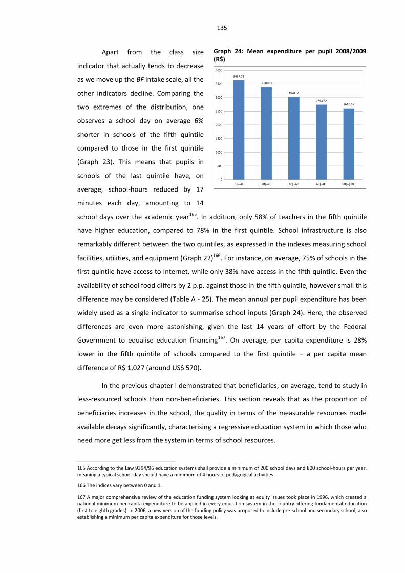
135
Apart from the class size
indicator that actually tends to decrease
as we move up the BF intake scale, all the
other indicators decline. Comparing the
two extremes of the distribution, one
observes a school day on average 6%
shorter in schools of the fifth quintile
compared to those in the first quintile
(Graph 23). This means that pupils in
schools of the last quintile have, on
average, school-hours reduced by 17
minutes each day, amounting to 14
school days over the academic year165. In addition, only 58% of teachers in the fifth quintile
have higher education, compared to 78% in the first quintile. School infrastructure is also
remarkably different between the two quintiles, as expressed in the indexes measuring school
facilities, utilities, and equipment (Graph 22)166. For instance, on average, 75% of schools in the
first quintile have access to Internet, while only 38% have access in the fifth quintile. Even the
availability of school food differs by 2 p.p. against those in the fifth quintile, however small this
difference may be considered (Table A - 25). The mean annual per pupil expenditure has been
widely used as a single indicator to summarise school inputs (Graph 24). Here, the observed
differences are even more astonishing, given the last 14 years of effort by the Federal
Government to equalise education financing167. On average, per capita expenditure is 28%
lower in the fifth quintile of schools compared to the first quintile – a per capita mean
difference of R$ 1,027 (around US$ 570).
In the previous chapter I demonstrated that beneficiaries, on average, tend to study in
less-resourced schools than non-beneficiaries. This section reveals that as the proportion of
beneficiaries increases in the school, the quality in terms of the measurable resources made
available decays significantly, characterising a regressive education system in which those who
need more get less from the system in terms of school resources.
165 According to the Law 9394/96 education systems shall provide a minimum of 200 school days and 800 school-hours per year, meaning a typical school-day should have a minimum of 4 hours of pedagogical activities.
166 The indices vary between 0 and 1.
167 A major comprehensive review of the education funding system looking at equity issues took place in 1996, which created a national minimum per capita expenditure to be applied in every education system in the country offering fundamental education (first to eighth grades). In 2006, a new version of the funding policy was proposed to include pre-school and secondary school, also establishing a minimum per capita expenditure for those levels.
Graph 24: Mean expenditure per pupil 2008/2009 (R$)

136
7.4 How do schools compare as to Bolsa Família participation and observed
outcomes?
Given the scenario described in the previous section, it is expected that a relationship
will be found between school outcomes and proportion of beneficiaries in schools. Graph 25
and Graph 26 (see also Table A - 26) confirm the expected trend for the mean test scores in
Mathematics and Portuguese Language on the 2007 national exam and for school
performance indicators (pass-grade and dropout rates) in the same year. Results in
Mathematics are consistently higher than in Portuguese Language across groups (Graph 25).
The gap between the first and fifth quintiles reaches some 27 points for Mathematics and 26
points in Portuguese Language; these figures roughly represent one cognitive level difference
in the proficiency scale168. In Graph 26 a drop in pass-grade rates of around 9 p.p. between the
extreme quintiles of schools is observed. The difference in dropout rates between the two
groups reaches 2.7 p.p., that is, a rate three times higher for schools with more than 80%
beneficiaries in relation to those with less than 20% BF intake.
School outcomes would not be significantly different, given the previously described
characteristics of schools with high BF intakes. Social disadvantage and school inequality add
to the reproduction of a vicious cycle in which poor children access poor education and end up
failing in the school system and in accessing better paid jobs in the future. However, as
mentioned earlier, BF beneficiaries are not concentrated in schools situated in the last two
quintiles of BF intake. In fact, only 25% of beneficiaries attend schools in which more than 60%
of their students take part in the programme, and these schools do not differ significantly in
168 In Chapter six I discuss three different ways of interpreting differences in test score achievements on the national exam.
16
0.0
017
0.0
018
0.0
019
0.0
020
0.0
0
Test S
core
0|--20 20|--40 40|--60 60|--80 80|--|100Proportion of BF intake
Portuguese Maths
4th grade - 2007
Test Scores in Maths and Portuguese
Graph 25: School achievement in test scores by BF intake (%)
1.5
2.0
2.5
3.0
3.5
4.0
Dro
pout
rate
(%)
82
84
86
88
90
92
Pass-g
rade r
ate
(%)
0|--20 20|--40 40|--60 60|--80 80|--|100Proportion of BF intake
Pass-grade rate Dropout rate
4th grade-2007
Pass-grade and Dropout rates
Graph 26: School performance indicators by BF intake (%)

137
terms of composition, resources, and results169, and are the least resourced in the system.
There is a distribution of beneficiaries across quintiles of schools by BF intake that could
attenuate the negative effects of school composition and school resources for a large
proportion of children participating in the programme. However, one must not forget that
one-quarter of beneficiaries study under the worst conditions available in the system.
7.5 Bolsa Família factors and school outcomes
Participation of children in BF differs across schools, not only in terms of the share of
students taking part in the programme, but also in relation to the length of time of
participation, the per capita cash transferred to families, and their level of poverty measured
by household per capita income. Therefore, I consider the correlation coefficients between
these BF factors and school outcomes as a first step in the analysis of the possible influence of
BF on school results.
Looking at the correlation coefficients between BF intake and school outcomes in
Table 21, a substantial negative correlation is observed for mean test scores and a moderate
correlation for pass-grade and dropout rates. A high proportion of BF intake is associated with
low performance at the school level, as measured by the mean test scores and mean pass-
grade and dropout rates. The mean household per capita income of beneficiary families170 is
positively correlated with school outcomes171. This result shows that differences in the level of
poverty amongst beneficiary families might influence school results.
169 See Graph 20 to Graph 26.
170 The indicator household per capita income in the data is measured only for BF households, therefore not reflecting the
average per capita income of all families whose children attend school, only the beneficiary families.
171 In the case of dropout a negative correlation coefficient implies a reduction in dropout rates with increases in household per
capita income representing an improvement in performance.

138
Table 21: Pearson’s correlation coefficient between BF factors and school outcomes
Bolsa Família variables at the school level School outcomes
% B
F in
take
BF
ho
use
ho
ld
per
cap
ita
inco
me
Tim
e o
f p
arti
cip
atio
n
Per
cap
ita
Cas
h T
ran
sfer
Pas
s-gr
ade
rate
Dro
po
ut
rate
Mat
hem
atic
s
Po
rtu
gues
e
% BF intake 1.00
BF household per capita income -0.33* 1.00
Time of participation 0.16* -0.23* 1.00
Per capita Cash Transfer 0.19* -0.71* 0.05 1.00
Pass-grade rate -0.24* 0.30* -0.10* -0.17* 1.00
Dropout rate 0.18* -0.26* 0.05* 0.16* -0.58* 1.00
Mathematics -0.45* 0.45* -0.14* -0.29* 0.36* -0.30* 1.00
Portuguese -0.47* 0.45* -0.15* -0.28* 0.38* -0.32* 0.93* 1.00
Note: Pairwise calculation with correlation coefficients statistically significant at 0.01% level indicated by *.
Table 21 also allows us to interpret another two key correlations between BF factors
and school outcomes. Time of participation and per capita cash transfer are negatively
correlated with all four indicators of school outcomes, that is, as the mean number of months
of participation in BF increases, the observed outcomes, on average, worsen. The same results
are seen for increasing values of per capita cash. The negative correlation with school
outcomes holds, even when analysed at different quintiles of BF intake as Table A - 27
describes for the case of test scores in Portuguese Language and time of participation in BF.
The last result seems to deny, from the outset, the hypotheses I test in this chapter;
that time of participation in BF and the cash value paid to families will be found as key
variables explaining potential positive effects of BF on children’s school outcomes. The
problem, however, is that face value correlation coefficients between two variables taken in
isolation can be misleading, since it does not allow for other possible interactions from factors
that can simultaneously affect both variables, producing a correlation coefficient that is not
only due to the examined relationship, but carries external influences as well. For instance,
because household per capita income is negatively correlated with time of participation172 (-
0.23), it might be that this correlation would bias the observed (negative) correlation between
time of participation and school outcomes. As per capita income decreases, school outcomes
also decrease, therefore, a longer time of participation masks low income as the driving force
behind poor school outcomes. The same happens with per capita cash, with a much stronger
172 An expected result considering that the higher the average per capita income for beneficiary families in a given school, the less likely those families were to have been prioritised in the registration process to take part in the programme, resulting in a shorter time of participation on average.

139
coefficient (-0.71), showing that the poorer the family the higher the per capita cash paid to
them173. A first useful way to control for multiple influences on the correlation coefficient
between two variables is to use partial and semipartial correlation coefficients.
As an example, Table 22 reports the partial and semipartial correlation coefficients
between the test scores in Portuguese Language and each of the BF factors examined. The
partial correlation coefficient expresses the correlation of each of the BF factors with test
scores, holding the others constant. The semipartial correlation discounts the mutual
influences of each BF factor on each other, while assessing their correlation with test scores. In
the case of time of participation in BF, the partial correlation coefficient is still negative but is
much closer to zero and below the conventional significance level. As to the coefficient for per
capita cash transfer, it becomes significantly positive. This means that the simultaneous
correlation of per capita income with test scores, time of participation in BF, and per capita
cash transfer were blurring the correlations with test scores of these two BF factors. It is
evident that even by employing a simple and rather crude approach, the initial negative
correlation of time of participation and cash with school outcomes dramatically changes. A
more sophisticated way of dealing with such confounding effects is to make use of multiple
regression analysis.
Table 22: Partial and semi-partial correlation coefficients between Portuguese Test Scores and BF factors
Variable Partial Corr. Semipartial
Corr. Significance
Value
% BF intake -0.37 -0.33 0.00
BF household per capita income
0.29 0.25 0.00
Time of participation
-0.01 -0.01 0.11
Per capita cash transfer
0.05 0.04 0.00
In order to explore further the relevance of time of participation and cash value on
school outcomes, in the next section I estimate several multiple regression models using cross-
sectional data, in which I explore potential effects and interactions between time of
participation and per capita cash on school outcomes and discuss potential causes of bias
influencing that relationship. Controls will be created in an attempt to purge those sources of
bias.
173 In fact, families below the extreme poverty line receive a fixed R$ 50 in additional to the variant component due to the
number of children in the family, potentially making the per capita cash higher for the poorest families.

140
7.6 The model and analysis
Using the cross-sectional data at the school level described earlier, I estimate a model
using multiple regression analysis in which I examine the marginal effect174 of the proportion
of beneficiaries in BF – moderated by time of participation and per capita cash value – on
school outcomes. The hypothesis to be tested is that although the proportion of beneficiary
students in schools is expected to be negatively correlated with school outcomes, due to what
has been called the “programme placement effect”, this trend would have diminishing
marginal effects across schools depending on the average time of participation in the
programme and also on the mean cash value paid to families. If confirmed, these trends will
signal a positive contribution of BF on school outcomes, going beyond the broadly explored
and disseminated positive effects on enrolment and attendance.
7.6.1 From the hypotheses to the econometric model
As the proportion of beneficiaries is thought to affect school outcomes, a simple
econometric model to describe and estimate that effect can be expressed as follows:
(I)
where Yi is the school outcome of interest for school i175, PropBFi is the proportion of
beneficiaries in a school i, and εi is the error term capturing the variation in the school
outcome not accounted for the variable PropBF. The coefficient α0 in this model is held
constant across schools and represents the average or expected value of the school outcome Y
when PropBF is zero. The coefficient α1 is also held constant and gives the marginal variation
on Y due to a unit increase in PropBF, that is, the “effect” of the proportion of beneficiaries on
school outcomes. In such a model, α0 and α1 are the parameters to be estimated.
In order to test the hypotheses of time and cash as two key factors moderating the
effect of PropBF on school outcomes (α1), these variables must be introduced in model (I). This
is done in two steps.
First, the parameter α1 is allowed to vary across schools by making it dependent on the
mean time of participation in each school. I make the effect α1 a linear function of the variable
174 “Marginal effects” is used here since it is normally referenced in the econometrics literature. The term “effect”, however,
does not necessarily mean causal effect. The “marginal effect” or simply “effect” of a variable X on Y is, in fact, the partial
derivative of Y in respect to X; that is, the marginal variation of Y associated with an infinitesimal change in X.
175 The subscript “i” indicating the unit of analysis (school) will be omitted to simplify the notation.

141
Time, which can be thought of here as the moderator or intervening variable, responsible for
changing the effect of PropBF on Y, as described in equation (II).
(II)
The coefficient δ2 gauges how the effect of PropBF on school outcomes changes by a unit
increase in the mean time of participation in BF. The coefficient δ1 gives the mean effect of
PropBF when time of participation is zero176. The error term ε1 is necessary to allow a non-
deterministic dependency of α1 on Time.
Likewise the coefficient α0 can also be expressed as a function of Time in order to allow
the intercept in expression (I) to vary across schools to reflect differences on the mean school
outcome derived from mean time of participation when the proportion of beneficiaries is
zero177.
(III)
Now substituting (II) and (III) into (I):
(IV)
Expression (IV) shows that making the effect of PropBF on Y conditional on Time
generates a model with an interactive term (PropBF x Time) and an error term
that will not have a constant variance across schools, since it depends on the
variable PropBF. As argued by Kam and Franzese (Kam and Franzese, 2007, pp. 128-129) the
heteroskedasticity (non-constant variance) can be easily addressed in the regression by using
the White’s procedure to generate a consistent variance-covariance matrix and, therefore, to
correct the coefficient-estimates’ standard errors in the estimated model178.
The second step is to integrate the variable Cash in the model. The hypothesis here is
that time of participation changes the effect of PropBF on school outcomes differently from
school to school depending on the level of cash paid to families in each school. This
176 Although unlikely in the data, it is technically possible that schools with beneficiaries have zero time of participation, since this
variable is measured as months of participation and beneficiaries with less than 30 days in the programme would allow such a
case to exist (there is only one school in the sample that fits this case).
177 It might be argued that allowing the intercept to vary with Time would make no practical sense, since it represents the mean
value for school outcome (e.g. test score) when the proportion of beneficiaries is zero. I will argue for the maintenance of a variant
intercept (α0) later in this chapter.
178 This is done in STATA using the option “robust” for the regression command.
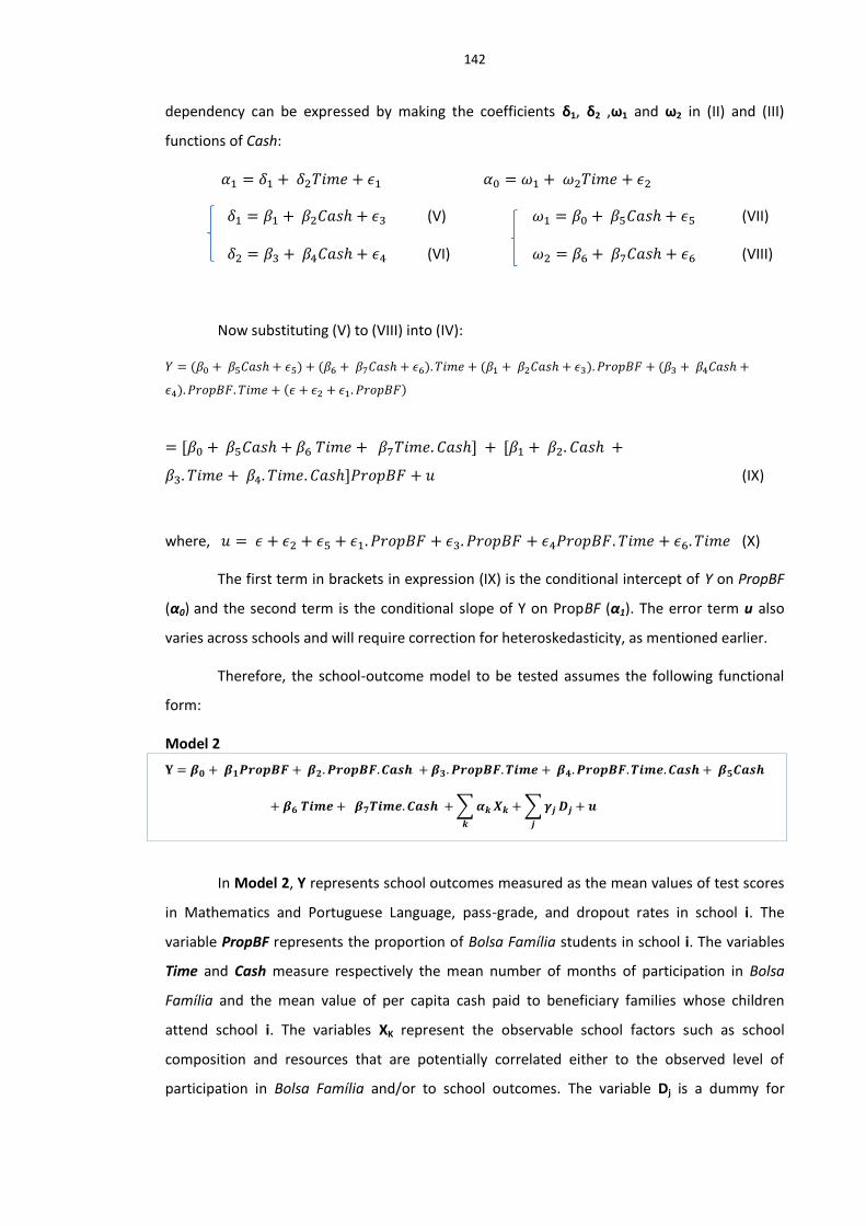
142
dependency can be expressed by making the coefficients δ1, δ2 ,ω1 and ω2 in (II) and (III)
functions of Cash:
(V) (VII)
(VI) (VIII)
Now substituting (V) to (VIII) into (IV):
(IX)
where, (X)
The first term in brackets in expression (IX) is the conditional intercept of Y on PropBF
(α0) and the second term is the conditional slope of Y on PropBF (α1). The error term u also
varies across schools and will require correction for heteroskedasticity, as mentioned earlier.
Therefore, the school-outcome model to be tested assumes the following functional
form:
Model 2
∑
∑
In Model 2, Y represents school outcomes measured as the mean values of test scores
in Mathematics and Portuguese Language, pass-grade, and dropout rates in school i. The
variable PropBF represents the proportion of Bolsa Família students in school i. The variables
Time and Cash measure respectively the mean number of months of participation in Bolsa
Família and the mean value of per capita cash paid to beneficiary families whose children
attend school i. The variables XK represent the observable school factors such as school
composition and resources that are potentially correlated either to the observed level of
participation in Bolsa Família and/or to school outcomes. The variable Dj is a dummy for

143
region. Finally, u represents the disturbance term capturing the variance in school outcomes
not explained by the variables included in the model.
Model 2 brings the three main factors associated with the BF programme at the school
level as explanatory variables of school outcomes: the share of pupils taking part in the
programme, the mean time of participation, and the mean cash transfer paid to families. It is
an interactive model since the key BF factors being analysed (PropBF, Time, and Cash) enter
into the model as product terms, meaning that these variables can be thought of as
moderators of each other. For instance, Time and Cash can be regarded as moderators of the
variable PropBF or, conversely, being moderated by PropBF and by one another, since the two
factors interact with each other. It is a symmetric model in which one variable (e.g. Time)
modifies, and in fact conditions, the effects of the other variables, and vice-versa.
In interactive models the estimated parameters cannot be directly interpreted as
effects (Kam and Franzese, 2007, pp.19-20). This means that coefficients β1 to β7 in Model 2,
taken in isolation, cannot tell us the estimated effects on the outcome Y. Each variable
involved in interaction terms has multiple effects, depending on the levels of the other
variables with which it interacts. For this reason, the estimated effects of each of the variables
of interest (PropBF, Time, and Cash) must be assessed using the conditional effects expressions
as described below.
Equation 1
Equation 2
Equation 3
These are simply the partial derivatives expressing the marginal effects of PropBF,
Time, and Cash on school outcomes. Taking, for instance, Equation 1 above, the effect of
PropBF on school outcomes Y is not given by the coefficient β1 as the mean estimated effect
for all schools. The role played by the other variables (Time and Cash) in the proposed model is
to moderate the effect the proportion of beneficiaries (PropBF) has on school outcomes,
making it change according to those two characteristics in each particular school. Equation 1
tells us that although the “programme placement effect” potentially has a negative effect on
school outcomes (it brings more disadvantaged children to school), the programme

144
mechanisms in operation through the cash transfer (reduction of immediate poverty) and the
conditionalities on health, nutrition, and education might potentially be positively contributing
to the improvement of school outcomes over time. This will empirically be supported if the
combination of the estimated β1, β2, β3, and β4 yields a positive and statistically significant
marginal effect of PropBF at some values of Time and Cash, or if a negative marginal effect of
PropBF can be proven to diminish across different values of Cash and Time.
Because interactive models with all the constitutive terms are mathematically
symmetrical, it is also possible to analyse the marginal effects of Time and Cash (as in Equation
2 and Equation 3) as being moderated by PropBF in each school and by one another. Both
directions of analysis are mathematically possible, although it seems more intuitive to think of
PropBF as the focus variable, whose influence on test scores is modified according to Time and
Cash. In fact, the reasoning I developed to construct Model 2 implicitly assumes this direction
of events: children in school first need to be registered in the programme (PropBF≠0); families
then start receiving a monthly per capita cash transfer (Cash≠0); and they receive the transfer
for a certain period of time (Time≠0)179. Besides, Equations 2 and 3 suggest that marginal
effects of Time and Cash might be estimated (in the case β5 or β6 were statistically different
from zero), even if the proportion of beneficiaries was zero. This sounds counterintuitive, since
no effect of Cash or Time should be expected when there are no beneficiaries in the school.
The above-mentioned difficulty with Equations 2 and 3 derives from the first term in
brackets of expression (IX). That term results from making the intercept in expression (I)
conditional on Time and Cash. It is worth noting that Equation 1 does not change if that term is
dropped from the model. Dropping that term from expression (IX) only changes Equations 2
and 3, which lose the first two terms, ) and ( ) respectively, the
parts predicting an implausible result. This might suggest the exclusion of that term from
expression (IX) to eliminate the implausibility and eventually work with Equations 2 and 3 as
well. However, allowing the intercept α0 in expression (I) to vary as function of Time and Cash
is statistically necessary. As I argue later in this chapter, it ensures that all constitutive terms180
are included in the model and thus circumvents bias in the estimated coefficients entering
Equation 1. Therefore, I consider PropBF as the variable whose effect on school outcomes is
moderated by the other two varying characteristics of BF in each school (Cash and Time),
making Equation 1 central to the analysis.
179 I followed a path in developing the model that brought Time and then Cash into the model, but the order in which these two
variables enter into the model is irrelevant once PropBF is fixed as the focus variable.
180 By “constitutive terms” I mean (following Kam and Franzese (2007)) all variables composing the interaction terms in the
model.

145
7.6.2 Selecting controls for families’ and schools’ characteristics
A set of covariates is also included in Model 2 (∑ representing variables to be
controlled for in estimating the model so to reduce the potential influence of omitted
variables. Omitted variables are variables not included in the model that can seriously bias the
estimation of any of the coefficients βk due to simultaneous correlations with the dependent
variable and one or more of the independent variables already in the model. In Section 7.3 I
described many school factors related to school composition and resources that might be
simultaneously correlated with school outcomes and the level of participation in BF181,
particularly with the variables being investigated (Time and Cash). If a particular observable
school characteristic affecting school outcomes such as geographic location is correlated with
BF factors and is not included in the model, the risk of bias in estimating β1, β2, β3, and β4
(parameters of interest to estimate the marginal effect of PropBF) increases considerably. For
example, the Northeast region is the least developed region in Brazil and its school outcomes,
on average, tend to be lower than for schools in the other regions. It is very likely that
municipalities in the Northeast were amongst the first to be mobilised and to have families
included in the programme due to its poverty levels. Consequently, the tendency is that
schools in that region have larger proportions of beneficiaries and also have longer mean times
of participation in the programme. These schools also tend to score lower in school
outcomes182. Therefore, the coefficients associated with marginal effects of BF participation on
school outcomes would be biased if regions were omitted from the model. Geographic
location is a relevant variable to be included in the model, as it potentially influences school
outcomes and also is correlated with the variables of interest183.
It might also be the case that unobservable variables influencing the level of
participation in the programme in each school would also be correlated with school outcomes.
For instance, the level of information amongst families in relation to their rights and the
possibility of registering for the programme could be driving the different proportion of BF
families in each school. Those differences in information probably reflect different levels of
181 In section 7.5 I discussed how correlation coefficients between BF factors and school outcomes could be affected by the
influence of other variables in a way that could even change the sign of the correlation.
182 For example, schools in the Northeast have an average of 52% of students participating in BF, mean time of participation of 31
months, and schools received 158 points in Portuguese test scores. The Southeast has 30% participation in BF, 28 months’ mean
time of participation, and 179 points in Portuguese test scores.
183 I also consider estimating separate models for each region, which allows the parameters of interest related to BF participation
and the coefficients on all the other variables included in the model to differ across regions.

146
knowledge and skills amongst parents in BF targeted families, that is, human capital gaps184.
Different levels of human capital amongst parents are also correlated with differences in the
quality of support children can have at home and, thus, with children’s school outcomes. As a
result, schools with high proportions of BF students may reflect those families with high levels
of human capital amongst the poor. The estimated effects of participation in BF on school
outcomes in this case would be biased upwards. A proxy variable to the level of information
should be included in the model to control for those differences in human capital amongst
parents. The proportion of parents holding post-primary education degrees at the school level
is available in the dataset and can be used as a proxy for human capital in this case.
The same reasoning can be extended to other variables that potentially influence
school outcomes and can also be correlated with participation in BF and/or with Time and
Cash. How can these variables be identified? Although an exhaustive identification of such
variables is not possible, I select those from the socioeconomic questionnaire of Prova Brasil
and from the National School Census that fall into that criterion to try to reduce the potential
bias in the estimates. First I identify the socioeconomic factors associated with participation in
BF and examine the partial correlation coefficients of these factors with school outcomes.
Then I look at a set of school characteristics and their partial correlation with BF participation
and school outcomes. The relevant controls to be included in Model 2 are those variables that
are correlated with participation in the programme and that are also correlated with any of the
school outcomes.
To identify the socioeconomic variables associated with participation in BF, I estimate
a logit model to test a set of socioeconomic characteristics of students and their families as
predictors of the probability of participation in BF185. From the 25 socioeconomic variables
tested, 14 were found to be statistically significant as predictors of participation in BF, from
which 13 are available in the 2007 dataset to be aggregated at the school level. Table A - 28
reports the partial correlation coefficients of the socioeconomic and school characteristics
with school outcomes186 and BF factors, and indicates those to be introduced as controls in
Model 2.
184 Gary Becker refers to search for information about incomes as one of the forms of human capital amongst others, such as
schooling, on-the-job-training, medical care, and migration (see Becker, 1993,p.11).
185 The logit model is estimated using the dataset of Prova Brasil 2005 from the previous chapter, since only in 2005 was
participation in Bolsa Família identified in the socioeconomic questionnaire.
186 Only 11 socioeconomic variables are reported in the table. Two variables (piped water at home and books at home) were not
included, as they are related to material conditions at home already captured by household per capita income and the durable
goods index.

147
All socioeconomic variables selected as predictors of participation in BF and school
factors correlated with BF have statistically significant partial correlation coefficients with at
least one of the school outcomes investigated (see Table A - 28). Initially, I considered all those
variables as controls in Model 2. However, there is a caveat: by including as controls those
variables correlated both with school outcomes and participation in BF, and which are also
expected to change as result of the policy being implemented, we risk neutralising the
expected effect of BF in the regression. This engenders what is called “over controlling”
(Wooldridge, 2009, p.203). In Table A - 28, three socioeconomic factors fall into this category:
the proportion of child labour, the overage rate, and the durable goods index. For instance, BF
cash transfers and conditionality on minimum school attendance rate create conditions to
reduce the propensity of child labour amongst beneficiary families. Since child labour
negatively affects school outcomes, one way in which BF could be effective in improving
students’ school achievements would be to reduce the propensity of child labour amongst
poor families. By including child labour as a control in Model 2, and considering the ceteris
paribus framework for interpreting regression results, we would attempt to measure BF effects
on school outcomes holding the proportion of child labour constant, that is, freezing one of the
variables that could be the one changing as a result of the programme and causing some
improvements to school outcomes. The same thinking can be extended to the overage rate
and the durable goods index variables. Finally, a control for the proportion of pupils sitting for
the exam in each school is also included in the model. This control is important, because it is
possible that schools with high BF intakes have lower rates of participation in the exam187. In
the last column of Table A - 28 I indicate the variables included as controls in estimating Model
2 and the full description of the variables entering Model 2 is presented in Table 23.
187 This can happen either if beneficiary students do to not turn up on the exam day, or if schools tend to be selective by
excluding some of the beneficiaries from taking part in the exam. In fact, the correlation coefficient is -0.1 (ρ=0.000) showing that
there is a small but significantly negative correlation between BF intake and the proportion of students sitting for the exam.

148
Table 23: Description of variables used to estimate Model 2
VARIABLES DESCRIPTION
Bo
la F
amíli
a Fa
cto
rs
PropBF Proportion of 4
th grade BF beneficiaries in the school.
Cash Mean per capita cash paid to BF beneficiary families of 4
th
grade pupils in the school. Time Mean number of months of participation in BF of 4
th grade
pupils’ families in the school.
Sch
oo
l Co
mp
osi
tio
n (
stu
den
ts’ a
nd
ho
use
ho
lds’
ch
arac
teri
stic
s)
BF households’ per capita income Mean household per capita income of BF beneficiary families of 4
th grade pupils in the school.
Prop. of Boys Proportion of boys amongst the 4
th grade pupils in the school
who sat for the national exam in 2007. Prop. of Non-whites Proportion of non-whites amongst the 4
th grade pupils in the
school who sat for the national exam in 2007. Prop. Pre-school Proportion of pupils who attended pre-school amongst the 4
th
grade pupils who sat for the national exam in 2007. Prop. Failed Proportion of pupils who have failed any grade in past years
amongst the 4th
grade pupils who sat for the national exam in 2007.
Prop. in Large Families (7 or more) Proportion of pupils who live in families with 7 or more
members amongst the 4th
grade pupils who sat for the national exam in 2007.
Prop. Fem. Headed Household Proportion of pupils who live in female headed households
amongst the 4th
grade pupils who sat for the national exam in 2007.
Prop Mothers with post-primary education
Proportion of pupils whose mothers have completed secondary school or College amongst the 4
th grade pupils who
sat for the national exam in 2007. Prop Fathers with post-primary education Proportion of pupils whose mothers have completed
secondary school or College amongst the 4th
grade pupils who sat for the national exam in 2007.
Prop. Students sitting for the exam Proportion of 4
th grade pupils in the school who sat for the
national exam in 2007.
Sch
oo
l Res
ou
rces
Class size Number of enrolments in classes with 4th
grade pupils divided by the number of classes with 4
th grade pupils.
School day (hrs./day) Mean number of hours in a school day for 4
th grade pupils.
Prop. Teachers with HE Proportion of teachers working in 4
th grade classes who have
higher education. Utilities index Index number ranging from 0 to 1 measuring whether the
school has access to: piped water, power supply, sewage, and garbage collection.
Facilities index Index number ranging from 0 to 1 measuring the availability
of school facilities amongst 13 items measured by the National School Census.

149
VARIABLES DESCRIPTION
Equipment index Index number ranging from 0 to 1 measuring the availability of school facilities amongst 9 items measured by the National School Census.
Expenditure per pupil 2008/2009 Average expenditure per pupil in fundamental education
calculated in the school system to which the school is administratively subordinated using available data for 2008 and 2009.
Reg
ion
s
1.North Dummy variable equal to 1 if the school is located in the North region.
2.Northeast Dummy variable equal to 1 if the school is located in the
Northeast region. 3.Central-West Dummy variable equal to 1 if the school is located in the
Central-West region. 5.South Dummy variable equal to 1 if the school is located in the
South region.
Test
Sc
ore
s
A2007Port School mean test score result in 2007 for Portuguese Language.
A2007Math School mean test score result in 2007 for Mathematics.
7.6.3 Results (I): Testing the model
Table 24 reports the results of the regression coefficients and robust standard errors
of test scores in Portuguese Language on BF factors at the school level once the controls
described earlier are applied. Column (1) reproduces the first simple model described in
expression (I), added with the control variables. Because it has no interaction term, a
straightforward interpretation of the coefficient β1 is possible. As expected, β1 is significant and
negative reflecting the “programme placement effect” resulting in the association between
schools’ high proportions of beneficiaries with low achievements on test scores. The model
predicts a reduction of one-tenth of a point on the mean test score in Portuguese Language by
increasing one percentage point in the proportion of beneficiaries in schools. Column (2)
includes in the model the variables of interest, Time and Cash, as interactive terms with the
proportion of beneficiaries (PropBF). These are the terms in the model whose coefficients
enter the expression for the marginal effect of PropBF. As mentioned earlier, this model
assumes that the intercept α0 in expression (I) does not depend on Time and Cash, and implies
the exclusion of the first two terms in Equation 2 and Equation 3, although not affecting
Equation 1. Column (3) includes all the constitutive terms of the interactions with PropBF

150
entering in Model 2 to test whether the exclusion of these terms from the model affects the
coefficients of interest β1 to β4.
Table 24: Regression of test scores (Portuguese Language) on Bolsa Família factors controlling for schools’ socioeconomic composition and resources.
(1) (2) (3) VARIABLES Portuguese Portuguese Portuguese
PropBF (β1) -0.109*** -0.216*** -0.385*** (0.004) (0.062) (0.089) PropBF x Cash (β2) 0.006* 0.012** (0.003) (0.005) PropBF x Time (β3) 0.005** 0.008*** (0.002) (0.003) PropBF x Time x Cash (β4) -0.000** -0.000* (0.000) (0.000) Cash (β5) -0.172 (0.137) Time (β6) -0.073 (0.080) Time x Cash (β7) -0.003 (0.005)
Controls Yes Yes Yes
Constant (β0) 161.109*** 161.193*** 169.115*** (1.320) (1.337) (2.836) Observations 33,857 33,805 33,805 Adjusted R-squared 0.523 0.522 0.523
Robust standard errors in parentheses *** p<0.01, ** p<0.05, * p<0.1
The coefficients in column (3) show that neither Time nor Cash (or Time x Cash) have
statistically significant coefficients (shaded area) if not interacting with the proportion of
beneficiaries in the model. At first glance, this can suggest that those terms can be excluded
from the model without causing any problem. In fact, as argued earlier, their exclusion would
yield a more intuitive expression for the marginal effects of Time and Cash by eliminating the
first two terms in Equation 2 and Equation 3, which suggest that even though PropBF=0
marginal effects of Time and Cash would still be expected. However, there are several caveats
to note. First, these variables are jointly significant, meaning that the null hypothesis of all
three coefficients being simultaneously zero can be rejected with a high level of statistical
significance188. Second, as argued by several authors (Friedrich, 1982; Brambor, Clark and
Golder, 2006; Kam and Franzese, 2007) once researchers use an interactive model, all
constitutive terms should be included, otherwise the risk of incurring in inferential errors
dramatically increases. This recommendation is supported even though the coefficients of
188 The F-test yields F=22.56 (p=0.0000)

151
some (or all) constitutive terms are not statistically distinguishable from zero (as is the case in
column (3)). The reason is that the other parameters of interest (β1 to β4) will be estimated
with bias if the constitutive terms are dropped from the model. As can be seen in Table 24
(column (2)), all coefficients on the remaining terms change either in size or significance if
Time, Cash, and Time x Cash are not included in the model. The bias is due to the fact that the
excluded terms are correlated with those remaining in the model189 and are also correlated
with test scores190. Finally, as argued earlier, the exclusion of those terms implicitly assumes
that the intercept of Y on PropBF (α0 in expression (I)) is not conditional on Cash and Time,
thereby imposing a fixed intercept into the model. The consequence is that the slope (α1) for
different values of Time and Cash will have to change to allow crossing at the same intercept
(α0), even though these changes of slopes are not the best fit to the empirical data. Given the
results in Table 24 and based on these arguments, I adopt Model 2 as described in column (3)
to estimate the coefficients on BF factors for all school outcomes.
Table 25191 reports coefficients and robust standard errors for different school
outcomes. Although the non-significance of the coefficients in columns (3) and (4) may raise
some doubt about the relevance of BF factors for the last two outcomes in Table 25, the test
for joint significance of those factors interacting with PropBF reject the null hypothesis of β1 to
β4 equal to zero. Due to the interactive model, the relevance of the remaining constitutive
terms, as argued earlier, rely on the role those terms have, if absent, in creating biased
estimates of β1 to β4. The estimated coefficients presented in Table 25 will be used in the
following section to assess the marginal effects of BF factors on school outcomes.
189 This should be obvious, since the remaining variables are interactions with those being dropped from the model.
190 Note that their coefficients in column (3) are not exactly zero and their magnitudes are comparable to the other coefficients.
191 Table A - 29 reports the coefficients and robust standard errors for all variables included in Model 2.

152
Table 25: Regression of school outcomes on Bolsa Família factors controlling for school composition and resources. (1) (2) (3) (4) VARIABLES Portuguese Maths Pass-grade Dropout
PropBF (β1) -0.385*** -0.390*** -0.071 0.001
(0.089) (0.101) (0.067) (0.028)
PropBF x Cash (β2) 0.012** 0.011** 0.004 -0.000
(0.005) (0.006) (0.004) (0.002)
PropBF x Time (β3) 0.008*** 0.007** 0.001 -0.001
(0.003) (0.003) (0.002) (0.001)
PropBF x Time x Cash (β4) -0.000* -0.000 -0.000 -0.000
(0.000) (0.000) (0.000) (0.000)
Cash (β5) -0.172 -0.290* 0.142* -0.020
(0.137) (0.159) (0.083) (0.035)
Time (β6) -0.073 -0.093 0.049 0.006
(0.080) (0.092) (0.047) (0.019)
Time x Cash (β7) -0.003 -0.003 -0.004 -0.000
(0.005) (0.005) (0.003) (0.001)
Controls Yes Yes Yes Yes
Constant 169.115*** 187.238*** 62.618*** 16.689*** (2.836) (3.244) (1.996) (0.895) Observations 33,805 33,805 33,805 33,805 Adjusted R-squared 0.523 0.491 0.320 0.294
Test for joint significance of coefficients on terms including PropBF Ho: β1= β2= β3= β4=0 F-test 172.5 139.6 5.735 22.27 Prob > F 0 0 0 0
Robust standard errors in parentheses *** p<0.01, ** p<0.05, * p<0.1
7.6.4 Results (II): Marginal effects of BF intake on school outcomes
How can the results in Table 25 be interpreted? What do they indicate about the
relevance of BF factors on school outcomes? As BF factors enter into the model in an
interactive form, we cannot have a straightforward interpretation of the meaning of the
coefficients βk in respect to school outcomes. Considering the ceteris paribus nature of the
regression analysis framework, it does not make any sense to ask for the effect of a unit of
change, for instance, in PropBF, while holding PropBF x Time and the other terms interacting
with PropBF constant. In this case, the slope of the relationship between school outcomes and
the proportion of beneficiaries (PropBF) in the school depends on the values of Time and Cash
as referenced in Equation 1 reproduced below.
The point estimation of the marginal effect will vary according to the estimated
coefficients β1 to β4 and in respect to the values of the moderator variables Time and Cash.
Every point estimation will have a confidence interval and significance level, both of which

153
require the estimated variance of the marginal effect of PropBF on school outcome ( (
)
)
in order to be calculated. This will also depend on the values of Time and Cash and is given by
the expression below192:
Equation 4
(
)
( ) ( )
( ) ( )
( ) ( )
( )
( ) ( )
( )
Therefore, in order to estimate the marginal effect given by Equation 1 for a particular
outcome (Y), a pair of values for Time and Cash must be chosen. A reasonable initial approach
is to estimate at “typical” values of the moderator variables in the sample of
schools. Table 26 shows the mean values and s.d. for school outcomes and BF factors
nationally and by region.
Table 26: Mean and standard deviation for school outcomes and Bolsa Família factors
Region Portuguese Maths Pass-grade
rate Dropout
rate PropBF Time Cash
North 162.8 177.7 85.1 4.0 41.2 27.6 18.2
12.8 13.1 12.4 5.5 19.4 6.2 2.6
Northeast 157.9 174.2 80.3 5.9 52.1 30.9 18.7
13.8 14.4 13.8 7.5 20.0 5.8 2.3
Central-West
174.1 190.5 90.5 2.5 32.1 25.9 16.6
14.7 15.9 9.2 4.8 18.5 6.0 3.0
Southeast 179.0 197.3 89.4 1.3 30.1 27.8 16.5
17.0 18.8 10.3 3.2 18.3 6.3 3.0
South 181.2 200.1 91.6 0.6 27.7 29.6 15.9
15.1 17.0 8.6 1.8 17.8 7.1 3.4
Brazil 171.5 188.9 86.9 2.8 37.1 28.8 17.2
18.2 19.9 12.1 5.4 21.4 6.5 3.1
Using Model 2193 to estimate the coefficients entering Equation 1 and Equation 4, the
marginal effect of PropBF on school outcomes can be estimated at the mean values of Time
and Cash at the national level and by geographic region as reported in Table 27.
192 The STATA command “lincom” calculates the point estimate, the standard error, and the degrees of freedom, which then can
be used to calculate the t-statistic and the level of significance.
193 When estimating by region, the covariate “region” is dropped from the model. When regressing pass-grade and dropout rates
test scores are included as covariates in the model.

154
Table 27: Marginal effects of PropBF on school outcomes by region estimated at the mean value of Cash and Time.
School outcome Brazil Regions
North Northeast Central-West Southeast South
Portuguese -0.110*** -0.075*** -0.069*** -0.122*** -0.099*** -0.173***
Maths -0.112*** -0.073*** -0.069*** -0.126*** -0.093*** -0.186***
Dropout rate -0.016*** - -0.024*** - - -
Pass-grade rate 0.011*** - 0.014** - - -
*** p<0.01, ** p<0.05, * p<0.1, - Not significant
Table 27 shows a “positive” marginal effect of PropBF on dropout and pass-grade
rates194 nationally and for the Northeast region. These are “positive” marginal effects in the
sense that, on average, in schools where beneficiary families have been participating in BF for
a period of about 2 1/2 years and receiving an average of R$ 17.2 per capita, the proportion of
beneficiaries in the school is correlated with more students being promoted and fewer
students abandoning school over the academic year. In other words, a higher proportion of
beneficiaries in those schools is not deteriorating those indicators, but improving them.
However, Table 27 also indicates that BF intake has a consistent negative marginal
effect, nationally and across regions, regarding school performance on the national exam for
both Portuguese Language and Mathematics, when estimated at the mean values of Time and
Cash195. This result both contrasts and seems to contradict the national positive marginal
effects of BF intake on pass-grade rates. It suggests that schools with proportionally larger
numbers of beneficiaries (after controlling for test scores) are not retaining proportionally
more students, although they hold poorer results on average for the national exam. If schools
with higher proportions of BF intake perform worse on the national exam, better pass-grade
rates would not be expected, at least where promotion is based on learning outcomes as
measured by the national exam196.
The result here says something different and allows us to raise some hypotheses. It
might be the case that poor social background expressed by participation in BF influences the
decision on grade-retention in the opposite direction than would be expected based on test
score results. Families’ socioeconomic conditions might play a role in smoothing schools’
194 Here, “positive” means that an increase in the proportion of beneficiaries is associated with a reduction in dropouts (negative
sign) and an increase in pass-grade rates (positive sign).
195 It is also clear that these effects are not different between the two disciplines. This is an expected result, since test scores in
Portuguese and Mathematics are strongly correlated (see Table 21, Pearson’s coefficient=0.93)
196 In fact, Table 21 shows positive correlation coefficients between pass-grade rates and mean test scores in both disciplines.

155
internal criteria for not promoting students. As a result, the pass-grade rate would be
“inflated” by a factor proportional to the share of students from disadvantaged socioeconomic
backgrounds. In this case, higher pass-grade rates associated with BF intake would not reflect
improvements in learning, but attenuation of the retention criteria due to socioeconomic
disadvantage. On the other hand, it is more likely that the reduction in the dropout rate due to
BF intake, as expressed by the negative marginal effect of PropBF (-0.016), is the factor
contributing to the increase in the pass-grade rate. In fact, since pass-grade, dropout, and
grade failure are complementary rates (their sum equals one), we can say that the marginal
reduction in the dropout rate must be followed by marginal increases in one or both of the
other two indicators. Because the marginal effect on pass-grade is smaller than the marginal
effect on dropout rate in absolute terms, one can conclude that both grade-failure and pass-
grade rates are increasing as a result of BF intake. It is a positive result in the sense that not
only are more pupils staying in school until the end of the academic year, but also in that more
students are being promoted to the next grade, even considering that the grade-failure rate
would be increasing as well.
What about the test scores? The marginal effects of PropBF on test scores in Table 27
are all negative, both nationally and across regions. Although the results presented in Table 27
provide some evidence of the partial effects on school outcomes associated with BF intake,
those are marginal effects estimated at just one point (mean values of Time and Cash)
amongst several possibilities. Equation 1 tells us that changes in the Cash value, for instance,
will produce different marginal effects with different statistical significances. In this sense, the
resulting marginal negative effect of BF intake on test scores nationally and across regions,
reported in Table 27, cannot be taken as a general result, only as the estimates calculated at
the mean values of Cash and Time. As stressed by Kam and Franzese (2007), it is misleading to
talk about “generally positive” or “generally negative” effects of variables involving linear
interactions based only on point estimates. In order to provide a more complete picture of the
marginal effects when estimating an interactive model, those authors strongly recommend the
use of graphs, in which the estimated conditional effects and confidence intervals are plotted
against a range of meaningful values of the conditioning variables.
Graph 27 shows the marginal effects of BF intake on Portuguese Language test scores
at the national level plotted against time of participation in BF, holding fixed the cash transfer
at its mean value (R$ 17.2)197. The dashed lines (hourglass shape) represent the 95%
confidence interval of the estimated partial effect ( ), which is plotted on the 197 Since the marginal effect depends on two variables, a two-dimensional graphical representation requires fixing one of them.
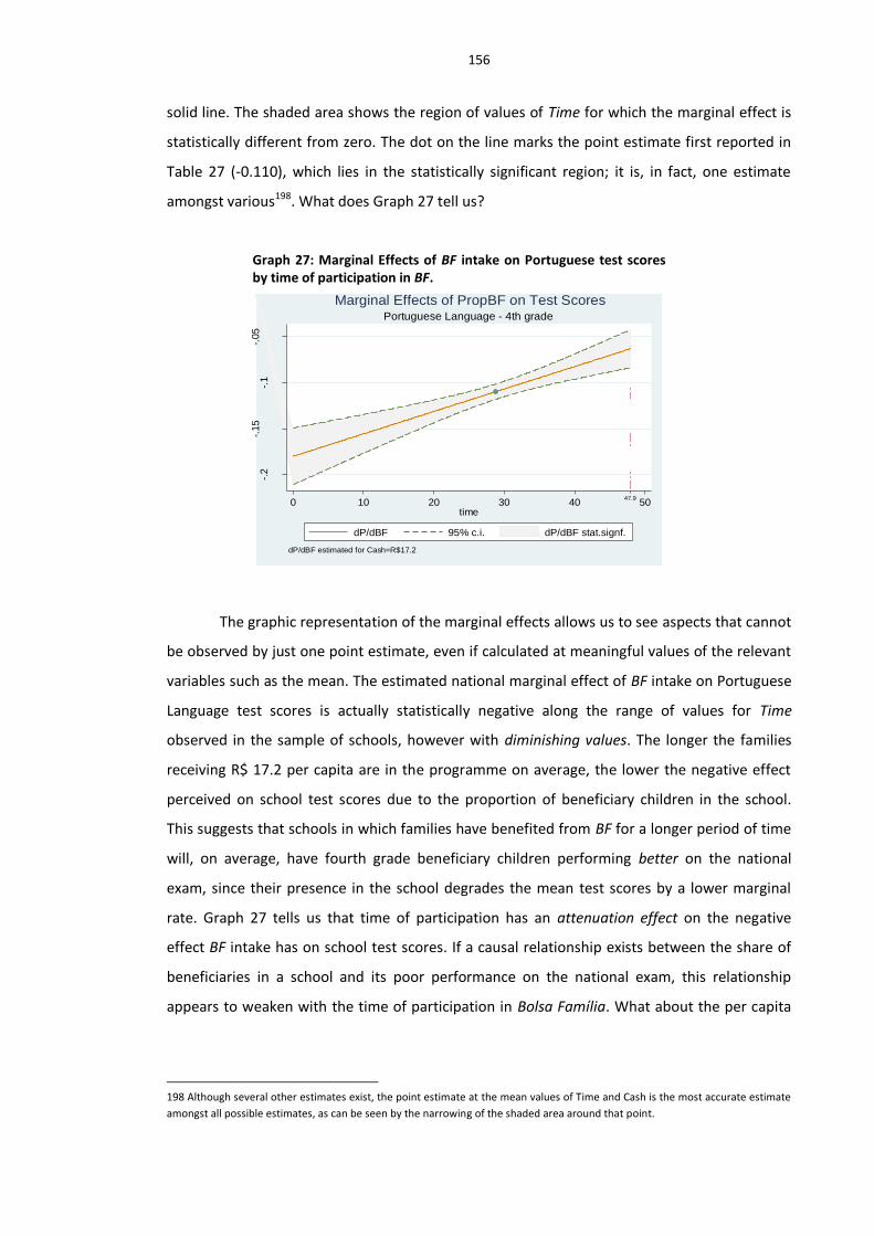
156
solid line. The shaded area shows the region of values of Time for which the marginal effect is
statistically different from zero. The dot on the line marks the point estimate first reported in
Table 27 (-0.110), which lies in the statistically significant region; it is, in fact, one estimate
amongst various198. What does Graph 27 tell us?
The graphic representation of the marginal effects allows us to see aspects that cannot
be observed by just one point estimate, even if calculated at meaningful values of the relevant
variables such as the mean. The estimated national marginal effect of BF intake on Portuguese
Language test scores is actually statistically negative along the range of values for Time
observed in the sample of schools, however with diminishing values. The longer the families
receiving R$ 17.2 per capita are in the programme on average, the lower the negative effect
perceived on school test scores due to the proportion of beneficiary children in the school.
This suggests that schools in which families have benefited from BF for a longer period of time
will, on average, have fourth grade beneficiary children performing better on the national
exam, since their presence in the school degrades the mean test scores by a lower marginal
rate. Graph 27 tells us that time of participation has an attenuation effect on the negative
effect BF intake has on school test scores. If a causal relationship exists between the share of
beneficiaries in a school and its poor performance on the national exam, this relationship
appears to weaken with the time of participation in Bolsa Família. What about the per capita
198 Although several other estimates exist, the point estimate at the mean values of Time and Cash is the most accurate estimate
amongst all possible estimates, as can be seen by the narrowing of the shaded area around that point.
-.2
-.15
-.1
-.05
47.90 10 20 30 40 50
time
dP/dBF 95% c.i. dP/dBF stat.signf.
dP/dBF estimated for Cash=R$17.2
Portuguese Language - 4th grade
Marginal Effects of PropBF on Test Scores
Graph 27: Marginal Effects of BF intake on Portuguese test scores by time of participation in BF.

157
cash? Does it also have a moderation effect on the negative association BF intake has on test
scores at the school level?
By estimating the marginal effect line described in Graph 27 for different values of per
capita cash, we can observe how Cash influences the BF intake marginal effect on Portuguese
test scores at the national level. Figure 8 shows the marginal effect lines for different
percentiles of Cash199. The point estimate (-0.110) is also plotted as a reference point200. The
scale on the vertical axis is fixed between -0.3 and +0.1 to allow the observation of changes on
the slope.
Figure 8: Marginal Effects of BF intake on Portuguese test scores by time of participation at different percentiles of per capita Cash.
Figure 8 shows the same trend of diminishing negative marginal effects along time of
participation for different values of Cash. It also indicates that for higher values of Cash, the
marginal effect line shifts up at the same time as its slope decreases. The shift upwards for
higher values of per capita cash suggests that the marginal effect of BF intake not only
decreases with time of participation, but also with increases in the value of the benefit201. For
199 The following percentiles are estimated: 5th, 25th, 50th, 75th, and 95th.
200 Graph 27 is replicated in Figure 8(c). Notice that the mean for cash coincides with the median.
201 Notice that the point estimate (-0.110) is below the marginal effect line for higher values of per capita cash and above for
lower cash values.
-.25
-.2
-.15
-.1
-.05
dP
ort
/ d
BF
47.9
0 10 20 30 40 50Time
Cash=R$12.2
(a)
-.2
-.15
-.1
-.05
dP
ort
/ d
BF
47.9
0 10 20 30 40 50Time
Cash=R$15.3
(b)
-.2
-.15
-.1
-.05
dP
ort
/ d
BF
47.9
0 10 20 30 40 50Time
Cash=R$17.2
(c)
-.16-.14-.12-.1
-.08-.06
dP
ort
/ d
BF
47.9
0 10 20 30 40 50Time
Cash=R$19.1
(d)
-.12-.11-.1
-.09-.08
dP
ort
/ d
BF
47.9
0 10 20 30 40 50Time
Cash=R$22.1
(e)

158
instance, schools with an average of 12 months of participation in BF with families receiving,
on average, R$ 15.3 per capita (25th percentile) have an estimated marginal effect due to the
proportion of beneficiaries equal to -0.166. Those schools where families receive R$ 19 per
capita (75th percentile) have an estimated marginal effect of -0.136. However, the slope of the
marginal effect line also diminishes as per capita cash increases. Thus, the rate at which the
marginal effect declines with time of participation is lower for higher values of cash. In other
words, Time loses its attenuation power over the marginal effect of BF intake as the benefit
value increases. This variation in the slope is given by the partial derivative of Equation 1 in
relation to Time as expressed below202:
Equation 5
A graphic representation of the decline on the slope of the marginal effect line, based
on the estimated coefficients β3 and β4 and cash values ranging within the available data, is
displayed in Graph 28. The higher the cash value, the lower the variation rate of the BF
marginal effect with time of participation. For values of Cash over R$ 24.80 per capita,
increases in time of participation will not have any positive influence in reducing the marginal
effect of BF intake. This result suggests the
existence of a threshold for the positive moderation
effect Time exerts on the marginal effect of PropBF.
This threshold lies on the 99th percentile, meaning
that less than 1% of the schools in the sample has
such high mean values for per capita cash transfer.
Therefore, a large majority of schools in 2007 were
still able to accumulate gains from time of
participation in BF.
The inverse can also be shown. A threshold
is also predicted by the model that limits the
moderation effect Cash has on the marginal effect of PropBF. For instance, instead of plotting
the marginal effect of BF intake against time of participation, Figure A- 1 plots it against per
capita cash. Each graph in Figure A- 1 shows the estimated marginal effect lines for different
percentiles of Time. It can also be seen that the model predicts decreasing negative marginal
effects over increasing values of Cash, although with diminishing slopes over the variable Time.
202 It is in fact the second derivative of Y on PropBF and Time.
Graph 28: Variation of the slope with cash value

159
At the 95th percentile of time of participation, the slope is negative, an indication that the
possible gains on the mean test scores due to increases in the value of the benefit have
reached (and outstripped) a threshold now defined by the variable Time. Equation 6 below
gives the variation rate of the marginal effect of BF intake (slope) with Cash, which depends on
Time. Graph 29 shows a positive slope that diminishes with time of participation, where
crossing zero when Time is equal to 37.2. Beyond this threshold, increases in per capita cash
will not have any positive influence in reducing the marginal effect of BF intake. This value lies
on the 90th percentile of the distribution of schools by Time so that there is only 10% of the
sample with higher values for that variable. This
suggests that 90% of the schools in 2007 were still
improving their average test scores had families
received more per capita cash over the previous
months or years of participation.
Equation 6
To understand the meaning of such
thresholds, we need to look again at Equation 5
and Equation 6. The negative estimated β4 in
Equation 5 indicates that as the value of the per capita cash transfer increases, the marginal
gains for test scores due to time of participation in BF is attenuated. Likewise, the negative
coefficient β4 in Equation 6 implies that as time of participation increases, the marginal gains
for test scores due to the per capita value of the benefit diminishes203. These are compensating
effects and can be interpreted in terms of the relative importance of these two BF factors for
improvements in test scores. For instance, time of participation in BF, as a generator of
eventual gains for the schools’ mean test scores, is increasingly of minor relevance as the value
of per capita cash transfer increases. In other words, by paying more to families in per capita
terms, the time lag necessary for a certain effect on test scores as a result of participation in
the programme will be shorter. On the other hand, for low per capita cash, time of
participation becomes more relevant for any improvement to be observed in test scores.
203 These relationships can also be inferred from Equation 2 and Equation 3 by rewriting those equations as:
⁄
⁄
Because β4 is negative, the slope measuring the variation of the marginal effect of Cash (Time) with BF intake decreases with
increases in Time (Cash).
Graph 29: Variation of the slope with time of participation

160
Therefore, the negative β4 suggests a substitute effect between these two BF factors, meaning
that policy-makers, by allowing a more generous stipend to families, will probably observe
improvements in test scores in a shorter period of time; conversely, by paying lower levels of
benefits, policy-makers will wait longer for the expected results.
So far we have seen that conclusions about marginal effects based only on point
estimates such as those described in Table 27 are misleading when interactions occur in the
model being tested. The conclusion that the proportion of beneficiaries has a constant
“generally negative” effect on test scores, based on the point estimates presented in Table 27,
is not correct. It assumes an invariant marginal effect regardless of the two programme factors
most likely to affect children’s performance at school: the per capita cash value paid to families
and the duration of the programme for those children. By examining the estimated marginal
effect of BF intake along a series of values of Cash and Time, our conclusion completely
changes. In fact, the results suggest that test scores are changing (improving), as consequence
of either the value of the benefit paid to families or the time spent in the programme. In order
to see more clearly the magnitude of these improvements, I will now look at the predicted test
scores in Portuguese Language based on the estimated model at different values of Time and
Cash.

161
7.6.5 Results (III): Predicted Test Scores and Bolsa Família factors
By analysing differences in predicted test scores across different values of BF intake,
per capita cash, and time of participation using the estimated Model 2, it is possible to infer
how influential BF factors are with respect to school achievement in test scores under different
combinations of BF factors. For instance, Figure 8(a) shows how the negative marginal effect of
BF intake decreases with time of participation while per capita cash is held at the fifth
percentile (R$ 12.2). The decreasing negative marginal effect is expected to translate into
diminishing gaps between schools with low and high BF intakes as time of participation
increases. This gap reduction is illustrated in Table 28, which shows the predicted values of
Portuguese Language test scores for different values of BF intake and Time, holding cash fixed
at R$ 12.20204 and the remaining covariates at their mean values. Reading down the first
column one sees that schools in which beneficiary children have been enrolled for one year in
BF, the estimated gap between the two extremes of the BF intake rank205 is -19.1 points in the
proficiency scale, while in schools where the mean time of participation reaches four years
204 The predicted values in Table 28 are representative of the Southeast region (the reference category in Model 2). The indicated
gaps will be the same for any region although the predicted test scores will vary. This is because the dummy variable Dj for region
enters the model as an additive variable only, not interacting with the term moderating the slope (α1) that characterises the
variation of test scores with BF intake. The dummy for region shifts the fitted model up and down, depending on the value of its
coefficient γj.
205 Although one could argue that the group of schools with 0% BF intake and 12 months of participation is a nonsense that group
can be thought of as representing those schools with a very low proportion of BF students (e.g. < 0.1%).
Table 28: Predicted Test Scores (Portuguese) by BF intake and Time of Participation in BF (Cash=R$12.20)
BF intake
(%) 12 24 36 48 ∆
0 181.7 180.4 179.1 177.8 -3.9
10 179.8 179 178.1 177.3 -2.5
20 177.9 177.5 177.2 176.8 -1.1
30 176 176.1 176.3 176.4 0.4
40 174.1 174.7 175.3 175.9 1.8
50 172.2 173.3 174.4 175.5 3.3
60 170.2 171.8 173.4 175 4.8
70 168.3 170.4 172.5 174.6 6.3
80 166.4 169 171.5 174.1 7.7
90 164.5 167.6 170.6 173.7 9.2
100 162.6 166.1 169.7 173.2 10.6
∆ -19.1 -14.3 -9.4 -4.6
Time of Participation (months)

162
that gap is just -4.6 points. This represents a 14.5-point reduction in the gap (76%) equivalent
to 0.85 s.d.206. By reading across each of the rows in Table 28, it is also noticed that in schools
where beneficiaries represent more than 30% of the students, a positive and increasing
difference in test scores is estimated between those with, on average, one and four years of BF
participation. The largest difference is estimated in schools in which all children are
beneficiaries in BF. The 10.6-point positive gap represents a gain of 0.62 s.d. in the mean test
score for those schools with four years in BF in relation to those with just one year.
The predicted values shown in Table 28 are plotted in Figure 9 with 95% confidence
intervals for the estimates included. This shows how the slope measuring the negative effect
of BF intake on test scores diminishes as time of participation increases. As Time increases, the
fitted line reduces its inclination indicating the attenuation effect of time of participation on
the negative relationship observed between BF intake and test scores. As consequence, a
reduction in the gap between schools at different levels of BF intake across different values of
Time is also detected.
206 See Table 26 for standard deviations of school outcomes. I use the values for the Southeast region since the estimates are
calculated for that region.
160
170
180
190
160
170
180
190
0 50 100 0 50 100
12 24
36 48
Predicted Test Score c.i.
Po
rt
%BF
Graphs by time
Cash=R$ 12.2
Predicted Test Scores(Port) by %BF
Figure 9: Predicted Test Scores (Portuguese) for different periods of participation in BF.

163
The reduction in the gap is better evaluated by overlapping the confidence intervals as
illustrated in Graph 30, in which the fitted lines for two different values of Time (12 and 48
months) are plotted together with their confidence intervals. It shows that not all differences
presented in each row of Table 28 are statistically significant. In fact, only values of BF intake
above 45% have estimated positive gaps that are statistically significant different from zero207.
As the proportion of beneficiaries increases the relevance of time of participation becomes
more and more discernible, since BF students tend to dominate the mean school test score.
For schools with very low proportions of beneficiaries, whatever happens to this group will not
affect the school mean in any meaningful way. In the context presented in Graph 30208 only
schools with more than 45% of students taking part in BF are likely to notice differences in the
mean test score over time.
So far I have explored the potential effect of BF on school outcomes based on an
interactive model in which three factors associated with participation in the programme were
considered: proportion of beneficiaries in school, mean time of participation, and mean per
capita cash paid to families. The model tested (Model 2) considered all schools in the sample,
i.e. schools in which those three factors are shown to be variable and influential on school
outcomes. Two of those factors (Time and Cash) were found to be moderators of the marginal
effect of BF intake in a way that suggests a positive effect of BF on school outcomes. In the
next subsection I analyse a subsample in which schools lie in the same quintile of BF intake
207 A statistically significant difference is also observed for values below 15%. However, it is very unlikely that in schools with less
than 15% BF intake any factor involving those participants will be of major relevance in determining school achievement in test
scores.
208 Schools with a mean cash of R$ 12.20 and household and school resources around the mean value.
Graph 30: Predicted Test Scores (Portuguese) for one and four years of participation in BF.
16
016
517
017
518
018
5
0 20 40 60 80 10015 45
PropBF
1 yr 4 yrs
Cash=R$ 12.2 (5th p.)
Predicted Test Scores(Port) by %BF

164
(the fifth quintile). For this subsample it is shown that one of the BF factors (BF intake) is not
relevant to school outcomes, since all schools are very similar in respect to that factor. The
direct effects of Time and Cash on school outcomes are then estimated using a simplified
version of Model 2.
7.6.6 Results (IV): Focusing on the 5th quintile of BF intake.
I now analyse a subsample of schools in which one of the BF factors – the proportion
of beneficiaries – can be considered constant across all schools in terms of its influence on
school outcomes. I take only schools from the fifth quintile of BF intake, that is, schools in
which more than 80% of pupils are beneficiaries in BF. By doing this, the interaction model
discussed in the previous subsections is simplified, as is the analysis of the marginal effects of
Time and Cash, since they will no longer depend on a third variables (on PropBF). The analysis
of marginal effects of Time and Cash on school outcomes for this subsample is also relevant
inasmuch as this is the less well-resourced group of schools and also the one in which pupils’
families come from the most disadvantaged socioeconomic backgrounds (as discussed in
section 7.3). Any significant positive marginal effect of BF factors on school outcomes will be
estimated in a far more adverse school context than in the previous section.
I start by testing the assumption that PropBF is not relevant for school outcomes in
schools of the fifth quintile. Using Model 2, I test whether the coefficients on terms involving
the variable PropBF are jointly significant. As reported in Table 29, the null hypothesis stating
β1=β2=β3=β4=0 is not rejected for all school outcomes. It is expected that in schools where
more than 80% of the students are beneficiaries, outcomes are not significantly influenced by
changes in the proportion of beneficiaries. Although not all students in these schools are
necessarily enrolled in the programme, a large majority of beneficiaries tend to determine the
mean school outcome. Therefore, the terms including PropBF can be excluded from the model.

165
Table 29: Regression of school outcomes on BF factors controlling for school composition and resources (5th quintile of BF intake) (1) (2) (3) (4)
VARIABLES Portuguese Mathematics Pass-grade Dropout
PropBF (β1) -0.808 0.093 3.306 -0.874
(2.403) (2.774) (2.478) (1.011)
PropBF x Cash (β2) 0.052 0.005 -0.184 0.030
(0.129) (0.150) (0.134) (0.056)
PropBF x Time (β3) 0.028 0.005 -0.094 0.025
(0.081) (0.094) (0.083) (0.033)
PropBF x Time x Cash (β4) -0.002 -0.000 0.005 -0.001
(0.004) (0.005) (0.005) (0.002)
Cash (β5) -2.415 0.469 16.777 -3.105
(11.495) (13.283) (11.881) (5.016)
Time (β6) -1.328 0.045 8.272 -2.486
(7.184) (8.288) (7.333) (2.943)
Time x Cash (β7) 0.077 0.000 -0.457 0.080
(0.388) (0.450) (0.398) (0.165)
Controls Yes Yes Yes Yes
Constant 188.216 147.056 -245.311 105.225 (214.904) (246.734) (219.735) (90.664)
Observations 1,277 1,277 1,277 1,277
Adjusted R-squared 0.297 0.256 0.195 0.156
Test for joint significance of coefficients on terms including PropBF
Ho: β1= β2= β3= β4=0
F-test 0.781 0.982 0.749 1.895
Prob > F 0.538 0.416 0.559 0.109
The model to be estimated then turns into a simplified version of Model 2 that
includes only two interacting BF factors – Cash and Time:
Model 3
∑
∑
The set of covariates is the same as in Model 2209 (see Table 23) and the intercept is
also allowed to vary according to region by the inclusion of the dummy variable Dj. Table 30
reports coefficients and robust standard errors on BF factors for different school outcomes, as
well as the F-statistic to assess the joint significance of those factors210. The results show that
the null hypothesis stating that BF factors are jointly insignificant as predictors of test scores in
Portuguese Language and pass-grade rates can be rejected (at the 5% level). In the case of test
scores in Mathematics, we cannot confidently reject the null hypothesis. It can be inferred that
BF factors are, in this case, irrelevant at the national level for test scores in Mathematics in
schools pertaining to the fifth quintile of BF intake. However, the null hypothesis is rejected for
209 As in Model 2 when regressing pass-grade and dropout rates test scores are included as regressor. Also, the dummy for region
is excluded when running the model for subsamples by region.
210 See Table A - 30 in the appendix for the full set of variables.

166
the Northeast (at the 10% level) and South regions (at the 0.1% level) if the test for
Mathematics is run by region (see Table A - 31).
In the case of dropout rate, at first glance the temptation is also to conclude for the
joint insignificance of BF factors at the national level, since the F-statistic also yields a rho value
above the conventional levels of statistical significance. However, here some caution is
needed. The fact that β2 is marginally significant (ρ=0.098) cannot be ignored211. As stressed by
Wooldridge (Wooldridge, 2009, p.149) it is statistically possible that a group of insignificant
variables is clustered with a significant variable, yielding a jointly insignificant result at the
conventional levels. Logically, if the hypothesis of β2=0 is rejected, even with marginal
confidence, an inconsistency is engendered if one does not likewise reject the null Ho:
β1=β2=β3=0, although the F-statistic may suggest the opposite. This conflict between the t-
test for an individual variable and the F-test for a group of variables cannot be resolved
without some critical judgement on the part of the researcher. I will, at this point, reject the
null (Ho) for dropout rates and move on to estimate the marginal effects of Time and Cash. If,
in fact, BF factors are not relevant for dropout rates at the national level, this will become
evident in the confidence intervals plotted with the estimated marginal effects of Time and
Cash in the forthcoming paragraphs. Moreover, the test run by region shows that the null
hypothesis can be rejected for the Northeast and Central-West regions at the 10% level (see
Table A - 32).
Table 30: Regression of school outcomes on Cash and Time (5th quintile of BF intake) (1) (2) (3) (4)
VARIABLES Portuguese Mathematics Pass-grade Dropout
Cash (β1) 2.258*** 1.024 0.445 -0.531
(0.826) (0.948) (0.902) (0.342)
Time (β2) 1.168** 0.485 -0.038 -0.329*
(0.503) (0.575) (0.558) (0.199)
Time x Cash (β3) -0.068** -0.034 0.004 0.015 (0.027) (0.031) (0.030) (0.011)
Controls Yes Yes Yes Yes
Constant 115.438*** 153.806*** 48.463** 28.554***
(17.502) (19.907) (19.018) (7.221)
F- statistic for the joint significance of
Bolsa Família factors (Ho:β1=β2=β3=0)
F(3,1252) =
3.45
F(3,1252) =
1.50
F(3,1250) =
2.86
F(3,1250) =
1.75
ρ = 0.0161 ρ = 0.2136 ρ = 0.0359 ρ = 0.1543
Observations 1,277 1,277 1,277 1,277
Adjusted R-squared 0.297 0.256 0.196 0.155 *** p<0.01, ** p<0.05, * p<0.1
211 Also β1 is not only sizable but is estimated with ρ=0.120.

167
As argued earlier, given the interactive nature of the model being tested, the
coefficients in Table 30 do not coincide with the effects of the variables involved in the
interaction (Time and Cash). The meaningful effects are, in fact, the marginal effects of Time
and Cash, which depend upon two coefficients and on the values of the other variable212.
The estimated marginal effects of Time and Cash on school outcomes (Y) are given by
the expressions:
Equation 7
Equation 8
The variances of the marginal effects are estimated by the expressions below, which
are used to calculate the standard errors of the estimated marginal effects213:
Equation 9
(
)
( ) ( )
( )
Equation 10
(
)
( ) ( )
( )
Once the coefficients β1, β2, and β3 are estimated for each school outcome, a set of
general hypotheses can be tested as to whether or not BF factors have any influence on school
outcomes. Three general hypotheses are tested for each school outcome214 at the national
level in relation to each BF factor (Time and Cash) for the schools on the fifth quintile of BF
intake: (i) Do BF factors affect the school outcome? ; (ii) Do BF factors improve the school
outcome? ; (iii) Do the effects of BF factors on the school outcomes depend on each other?
Table 31 describes the hypothesis to be tested for each school outcome and BF factor, the
statistical test used, the result, and the conclusion.
212 The same happens to the variance of the marginal effects, upon which the statistical significance of the estimated marginal
effects depend.
213 Again, the STATA command “lincom” does the job of generating the estimates for the marginal effect as well as the standard
error and degrees of freedom so to allow the statistical significance to be calculated.
214 All school outcomes are tested except for the test scores in Mathematics, since we failed to reject the null hypothesis
(β1=β2=β3) at the national level in that case.

168
Table 31: Hypothesis tests for effects on school outcomes School
outcome (Y)
Bolsa Família factor
Hypothesis to be tested
Ho (Null hypothesis):
Test Result Conclusion
Test
Sco
re in
PO
RTU
GU
ESE
Cas
h
Does Cash affect test score?
β1= β3=0 F-test F=3.878
Prob. > F = 0.0209 Cash affects test
score.
Does test score increase with
Cash? β1+ β3.Time ≤ 0
Multiple t-tests (for
each value of Time)215
Multiple results to be assessed by plotting the marginal effects
of Cash across different values of
Time.
(Discussed in the text)
Does the effect of Cash on test
score depend on Time?
β3=0 t-test t=-2.52
Prob. > |t| = 0.012
The effect of Cash on test score
depends on Time.
Tim
e
Does Time affect test score?
β2= β3=0 F-test F=4.073
Prob. > F = 0.0173 Time affects test
score
Does test score increase with
Time? β2+ β3.Cash ≤ 0
Multiple t-tests (for
each value of Cash)216
Multiple results to be assessed by plotting the marginal effects
of Time across different values of
Cash.
(Discussed in the text)
Does the effect of Time on test
score depend on Cash?
β3=0 t-test t=-2.52
Prob. > |t| = 0.012
The effect of Time on test score
depends on Cash.
PA
SS-G
RA
DE
RA
TE
Cas
h
Does Cash affect pass-grade
rates? β1= β3=0 F-test
F=4.286 Prob. > F = 0.0140
Cash affects pass-grade rates.
Does pass-grade rate improve with Cash?
β1+ β3.Time ≤ 0
Multiple t-tests (for
each value of Time)217
Multiple results to be assessed by plotting the marginal effects
of Cash across different values of
Time.
(Discussed in the text)
Does the effect of Cash on pass-
grade rate depend on
Time?
β3=0 t-test t=-0.14
Prob. > |t| = 0.892
The effect of Cash on pass-grade rate does not depend
on Time.
Tim
e
Does Time affect pass-grade
rates? β2= β3=0 F-test
F=0.161 Prob. > F = 0.851
Time does not affect pass-grade
rates
Does pass-grade improve with
Time? β2+ β3.Cash ≤ 0
Given the previous
result no test is needed.
N/A
Since Time does not affect pass-grade
rate the latter cannot improve
either.
Does the effect of Time on pass-
grade rate depend on
Cash?
β3=0 t-test t=-0.14
Prob. > |t| = 0.892
The effect of Time on pass-grade rate does not depend
on Cash218.
215 As stressed by Kam and Franzese (2007), in the context of linear-interactive models, hypotheses tests for the sign of the
dependency tend to be ambiguous since the estimated value (e.g. β1+ β3.Time) might be positive, negative, or null depending on
the values of the variable interacting (e.g. Time). For this reason, the assessment of how test scores vary with Cash will be
assessed using graphs for marginal effects, as developed in the previous subsection.
216 See note 218.
217 See note 218.
218 This test is also unnecessary given that the first test had already failed to reject the null hypothesis leading to the conclusion
that Time has no effect on pass-grade rate. Since Time has no effect on pass-grade rate this effect does not exist and therefore
cannot depend on anything else.

169
School outcome
(Y)
Bolsa Família factor
Hypothesis to be tested
Ho (Null hypothesis):
Test Result Conclusion
DR
OP
OU
T R
ATE
Cas
h
Does Cash affect dropout rates?
β1= β3=0 F-test F=1.33
Prob. > F = 0.2649
Cash does not affect dropout
rates.
Does dropout rate decrease
with Cash? β1+ β3.Time ≥ 0
Given the previous
result no test is needed.
N/A
Since Cash does not affect dropout rates
the latter cannot decrease either.
Does the effect of Cash on
dropout rate depend on
Time?
β3=0
Given the previous
result no test is needed.
N/A
Since Cash does not affect dropout rates
the latter cannot depend on Time.
Tim
e
Does Time affect dropout rates?
β2= β3=0 F-test F=2.47
Prob. > F = 0.0852 Time affects
dropout rates
Does dropout decrease with
Time? β2+ β3.Cash ≥ 0
Multiple t-tests (for
each value of Cash)219
Multiple results to be assessed by plotting the marginal effects
of Time across different values of
Cash.
(Discussed in the text)
Does the effect of Time on
dropout rate depend on
Cash?
β3=0 t-test t=- 1.38
Prob. > |t| = 0.168
The effect of Time on dropout rate
does not depend on Cash.
For Portuguese Language we can confidently reject the null hypothesis of no effect of
Time and Cash on test scores and also conclude that the effects of Time on test scores depend
on the level of Cash and vice-versa. As to whether those effects are associated with
improvements on test scores can only be assessed at particular values of each BF factor upon
which the marginal effect depends (to be assessed later in this section). Pass-grade rate seems
to be affected by Cash, but not by the mean time of participation in BF, and the effect of Cash
does not depend on the value of Time either. In other words, time of participation turns out to
be irrelevant to pass-grade rates and also does not change the effect that Cash has on that
outcome. The sign of that effect can be assessed later using graphical analysis. Finally, dropout
rate is not affected by the value of cash, but we can marginally reject the hypothesis of no
influence of Time (at the 10% level). The effect of Time does not depend on the value of cash
and its direction is better assessed using graphical analysis later in this subsection220.
The hypotheses tested do not give us any idea about the size of the effects of Time and
Cash on school outcomes when they happen to be considered statistically different from zero.
One way of looking at the size of the marginal effects estimates given by Equation 7 and
Equation 8 nationally and regionally is by estimating those effects at meaningful values of the
219 See note 218.
220 I do not develop the same set of hypotheses step-by-step as I did for the national level by region. The results by region are
reported for the point estimates, in the same way I presented in section 7.6.4, in Table 33.

170
variables upon which they depend. For instance, taking the mean values of Cash and Time
nationally and by region for schools in the fifth quintile of BF intake (Table 32), the estimated
marginal effects of Time and Cash and level of significance are reported in Table 33221.
Table 32: Mean and standard deviation of school outcomes and Bolsa Família factors in schools of the fifth quintile of BF intake
Region Portuguese Mathematics Pass-grade rate
Dropout rate
Time Cash
North 159.1 175.2 83.0 4.3 27.6 17.8 12.1 11.9 14.2 6.0 5.6 2.1
Northeast 154.7 171.4 80.9 4.9 31.8 18.6 13.3 14.6 13.2 6.8 5.4 2.0
Central-West 168.3 184.3 91.0 2.1 25.7 17.6 13.4 14.8 9.3 3.5 5.7 2.7
Southeast 169.2 188.9 86.2 1.7 30.8 16.7 15.1 18.1 14.4 2.8 5.8 1.9
South 164.9 182.9 86.5 0.9 31.9 17.5 12.4 15.3 13.9 3.1 5.9 1.9
Brazil 158.0 175.0 82.4 4.1 31.1 18.2 14.5 16.3 13.6 6.2 5.8 2.2
Table 33: Marginal effects of Time and Cash on school outcomes by region, estimated at the mean values of cash and time for schools in the fifth quintile of BF intake
*** p<0.01, ** p<0.05, * p<0.1, - Not significant
Although the point estimates in Table 33 are insufficient to assess the whole of the
marginal effects associated with BF factors222, they allow us to gauge the magnitude of those
effects and see how they differ across regions for particular values of Time and Cash. For
instance, at the national level, the marginal effect of Time on dropout rates (-0.061) suggests
that, for schools in which the mean value of cash paid to families is R$ 18.20, each additional
10 months of participation in the programme is associated with a reduction of 0.6 p.p. in the
dropout rate. As I did not reject the hypothesis of β3=0 in Equation 8 for time of participation
221 The shaded areas mark the “positive” marginal effects, that is, those effects associated with improvements in school
outcomes.
222 As argued in subsection 7.6.4 they are only one amongst several estimates that can be more properly assessed by graphical
analysis.
North NortheastCentral-
WestSoutheast South
TimeBF - - - - - -
CashpcBF - - - - - -
TimeBF - - -0.190** - - -
CashpcBF - - - - - -3.010***
TimeBF -0.061* - - - - -
CashpcBF - - - -0.908** - -
TimeBF - - - - - -
CashpcBF 0.570*** - 0.420* - 2.209*** -
Pass-grade
rate
School
outcome
Portuguese
Maths
Dropout
rate
Bolsa
Família
factor
Brazil
Regions

171
(see Table 31), I conclude that the marginal effect of Time on dropout does not depend on the
level of cash paid to families for that group of schools. This does not mean that the estimated
effect of time will occur for every value of cash223, but that when the marginal effect of Time is
different from zero this will not differ across different levels of cash, and one can assume that
the estimate at the mean value of cash (0.061) is the national mean effect of Time on dropout
rates for schools with a large majority of pupils registered in BF. Likewise, the national
marginal effect of Cash on pass-grade rates does not depend on Time. Therefore, the
estimated marginal effect (0.570) at the mean value of time (31 months) represents the
national average effect of a unit increase of per capita cash on pass-grade rates for children
attending the most disadvantaged schools, independent of how long they have been in the
programme. One real (R$) increase in the per capita cash value is associated with a 0.6 p.p.
increase in pass-grade rates. This estimate gives us a significant and high associated effect of
Cash on pass-grade rates for those schools in which that indicator is the lowest observed
amongst schools (see Graph 26).
Across regions we can also observe significant marginal effects of Cash on pass-grades
and dropout rates. In the Central-West, a reduction of 0.9 p.p. in dropouts is estimated for an
increase of one real (R$) in the mean per capita cash paid to families in schools of the region
with a mean time of participation of 26 months. In the Northeast, a marginal effect on pass-
grade rates of a 0.4 p.p. increase for each additional real (R$) on the mean value of per capita
cash paid in schools of the region is estimated at a 10% significance level. In the Southeast, the
marginal effect of Cash is estimated with high level of significance and is also the highest,
suggesting an increase of 2.2 p.p. in pass-grade rates for a one real (R$) increase in mean per
capita cash224. Again, these are only point estimates at the mean values of Cash and Time and
cannot translate the whole picture of how those effects vary according to changes in those
variables.
In the same way, the predominant absence of significant marginal effects of Cash and
Time for test scores nationally and across regions in Table 33 cannot be taken as a general
result. Not only do both Cash and Time affect test scores in Portuguese Language at the
national level (see Table 31), but those variables also affect each other’s effects on test scores.
It is possible that the effects of BF factors are also detectable for test scores in Mathematics if
223 I will show later the interval of cash values for which the marginal effect of time is statistically different from zero.
224 One can raise the question why there is a higher effect in the Southeast compared to the Northeast. Perhaps better school
conditions in the Southeast play a role in the final results of beneficiaries.

172
the analysis is drawn from the national to the regional225. As discussed earlier, by looking at
single point estimates alone, one can draw incorrect conclusions about the relevance of BF
factors for school outcomes. Therefore, in the following paragraphs I present the marginal
effect lines of each BF factor at the national level for different school outcomes.
7.6.6.1 Test Scores
The full description of the marginal effects reported in Table 33 requires graphical
representation of Equation 7 and Equation 8, including the confidence intervals at each
estimated point. This means that for each cell in Table 33 a graph is needed226 to show the
variation of the marginal effect. The interval of values for which the marginal effects are
estimated is also limited to the real range of the values of Time and Cash in the sample of
schools in the fifth quintile (Table A - 33 and Table A - 34). Graph 31 and Graph 32 show the
marginal effect lines of Cash and Time on test scores in Portuguese Language at the national
level.
225 Remember that results in Table 31 are valid only for the national level and that, in the case of Mathematics, the test by region
revealed joint significance of β1, β2, and β3 for the Northeast and South regions (Table A - 31), which explain the two significant,
although negative, marginal effects estimated for Mathematics in Table 33 in those regions.
226 I display here only the marginal effect lines for the national level.
-2-1
01
23
27.310 20 30 40 50
time
dP/dC 95% dP/dC stat.signf.
dP/dC estimated for the 5th quintile of BF intake
Protuguese Language- 4th grade
Marginal Effects of CASH on Test Scores - NATIONAL
Graph 31: Marginal Effects of CASH on Portuguese Test Scores
-1-.
50
.51
19.4 25.310 15 20 25
cash
dP/dT 95% dP/dT stat.signf.
dP/dT estimated for 5th quintile of BF intake
Portuguese Language - 4th grade
Marginal Effects of TIME on Test Scores - NATIONAL
Graph 32: Marginal Effects of TIME on Portuguese Test Scores

173
Based on the range of significant estimates in Graph 31, it can be argued that in
schools of the fifth quintile of BF intake the value of per capita cash paid to poor families not
only affects test scores in Portuguese Language, but it does so in a positive direction227. The
significant marginal effects vary between 1.67 when time of participation is around 9 months
(the minimum value) to 0.42 when time is around 27 months (25th percentile), a four-fold drop
across the range of values for time of participation. This shows a diminishing marginal effect of
Cash with Time, the rate of which is given by the estimated coefficient β3 in Table 30 (-0.068).
The slope in Graph 31 describes that trend. The question of whether test scores in Portuguese
Language increase with cash (raised in Table 31) can now be answered by analysing the
interval in which the marginal effect line in Graph 31 is significant and positive, which is the
case for values of Time below 27 months. As expressed in Equation 7, the partial effect of Cash
depends on the initial value of Time at which it is estimated. The longer families have been in
the programme, on average, the lower the expected gain in test scores (Portuguese) due to a
one real increase in the per capita cash for those families. This result suggests that potential
positive effects on test scores due to increases in the per capita cash transfer to families are
constrained by a timeframe within which that policy is more likely to generate educational
benefits. The maximum gain from cash transfer increments on test scores would materialise if
it occurred at early stages of participation in BF. Even in less well-resourced schools, such as
those with more than 80% of children enrolled in BF, the analysis so far suggests that children
would benefit educationally from higher values of cash transferred to their families through
higher test scores on the national exam, provided that any increase in cash occurs before they
have been enrolled in BF228, on average, for 27 months.
Graph 32 shows a decreasing marginal effect of Time along values of per capita cash.
Although the estimates are positive for the initial range of cash values, they are not statistically
distinguishable from zero (at a 5% level of significance) for values lower than R$19.40, and
becomes negative above that threshold. This threshold corresponds to the 72nd percentile in
the subsample of schools analysed here. Therefore, for a large majority (72%) of schools, the
marginal gain from time of participation seems to be irrelevant and has a negative contribution
227 This result shows us again how misleading point estimates, such as those presented in Table 33, can be if taken as general
conclusions about the effects of interactive variables.
228 A clear limitation of Model 3 is to not account for the possibility that such marginal gains from increases in per capita cash
may not be the same for every level of household per capita income or for every cash value transferred to families. It is likely that
the marginal effect of cash diminishes with both household per capita income and current value of cash transfer. This non-linear
change of the marginal effect of cash would reflect the idea that one extra real (or dollar) would benefit poor children more than it
would benefit less poor children.

174
for those above the mean value of R$ 19.40 per capita. How do the two marginal effects (of
Cash and Time) combine to change results in schools of the fifth quintile of BF intake?
The reasoning behind marginal effects can be counterintuitive at times, so it is worth
exploring an example to clarify their implications for test scores229. Consider two schools, A
and B, from our group of high BF intake schools. In 2007, the year of the national exam, these
two schools have equivalent school composition and school resources in terms of the variables
described in Table A - 30 (these variables are fixed at their mean values). They are also located
in the same region in Brazil (Southeast). Assume that both schools have families with an
average of 24 months of participation in BF by the time they take part in the national exam.
During the previous two years before the exam, however, the two schools experienced
different courses of benefits paid to families. In school A, families were paid an average of R$
13.60 per capita/month230 over their entire period in BF. In school B, families had an increase
in the benefit after 12 months of enrolment in the programme, increasing the average per
capita cash to the 95th percentile of the distribution (R$ 19.70). How would this affect their
outcomes?
Differences in test scores in Portuguese Language obtained by schools in 2007 are
predicted according to finite changes in Time and Cash by the following expressions:
Equation 11
Equation 12
In 2007, School A has two years of participation over which families received an
average of R$ 13.60, as depicted below.
Ex. 1 School A:
c0=R$13.60 c0=R$13.60
t0=0 (Nov2005) t1=12 months (Nov2006) t2=24 months (Nov2007)
By plugging the estimated coefficients (β2 and β3), the per capita cash (c0), and the
period of participation in BF over which the families received the cash transfer (t2-t0) into
229 References to test scores in this subsection refer to achievements in Portuguese Language unless otherwise specified.
230 This is equivalent to the fifth percentile of the per capita cash distribution in the Southeast (see Table A - 33).

175
Equation 11, one can estimate the expected difference in test scores in 2007231 due to the
combined effects of time of participation and cash transfer.
School A is expected to have a mean test score in Portuguese Language that is 5.84
points higher than a school from the same group that has just started in BF in 2007, with
families receiving the same cash (c0)232.
Families in School B had an increase in their benefit, raising the average per capita
cash at the school level to R$ 19.70 after 12 months in BF, as represented below.
Ex. 2 School B:
c0=R$13.60 c1=R$19.70 c1=R$19.70
t0=0 (Nov2005) t1=12 months (Nov2006) t2=24 months (Nov2007)
We now need both equations to estimate the gain in test scores, since both Time and
Cash change for school B. The increase in cash after 12 months splits the period into two parts
and three contributions to test scores have to be estimated as follows:
Between t0 and t1:
At t1:
Between t1 and t2:
The resulting gain in test scores for school B is given by adding up the partial
contributions:
School B is expected to have a mean test score in Portuguese that is 9.66 points higher
than a school from the same group that has just started in BF, receiving, on average, R$ 13.60
per capita per family. Notice that the estimated gain in test scores due to the increase in per
capita cash in Nov 2006 will have a “discount” over the next 12 months by an amount
proportional to the second term in the programme, as shown by the negative value of ∆Y3.
Nevertheless, the model still predicts a gain in test scores for school B that is 3.82 points higher
than school A, suggesting that the mid-term variation in Cash contributes positively to test
scores in school B. If the raise of cash for school B in November 2006 had achieved a value
231 Notice that because there was no change in the value of cash over the period we do not need equation 12, since there are no
predicted gains due to variations in the per capita cash to be estimated.
232 In this example I am not considering the statistical significance of the expected difference in test scores, which will be
assessed later in this subsection.

176
lower than the threshold of R$ 19.40, the estimated ∆Y3 would not have been statistically
different from zero233, meaning that the “discount” would not have applied to the gains in test
scores due to the increase in cash234. On the other hand, if the change in the value of cash had
occurred after school B had completed an average of 27 months of participation in BF, it would
have a null contribution to gains in test scores in 2007, since that value of Time delimits the
zone of statistically positive marginal effects of Cash (see Graph 31). This example illustrates
how BF factors, through marginal effects, are associated with expected differences in test
scores, also explaining how those factors interfere with each other by attenuating one
another’s effect.
Table 34 reports a set of finite estimated differences in test scores and level of
statistical significance for changes in time of participation, evaluated at different levels of per
capita cash235. The values of cash range from the minimum to the maximum figures found in
the national sample of the fifth quintile group. As anticipated in Graph 32, for values of per
capita cash higher than R$ 19.40 [for which the marginal effect of time is statistically
significant (and negative)] the estimated differences in test scores are also found to be
statistically significant. It can be seen from Table 34, for instance, that the difference in test
scores ∆Y1 (=2.92) estimated in Ex. 2 (for cash=13.60 and ∆time=12) lies somewhere in the
third row, between the minimum value and p5, and is not statistically significant236. Likewise,
in the same example (Ex. 2), the estimated difference ∆Y3 (=-2.06) for cash=R$ 19.70 and
∆time=12 is close to the estimated value in the third row and fifth column of Table 34 (=-1.9)
and is statistically significant.
Table 35 reports the estimated differences in test scores for increases in per capita
cash by fractions of one s.d. (of the national sample) at different levels of Time, ranging from 0
to 48 months237, and level of statistical significance. Taking, for instance, the estimated
difference ∆Y2 (=8.80) from Ex. 2, it can be located in Table 35 somewhere in column five
(time=12) between the two last rows, indicating a significance level of 1% for that estimate.
233 It is because the marginal effect of time is not statistically different from zero below that threshold, as shown in Graph 32.
234 Notice also that the estimated ∆Y1 is also not statistically significant because the cash value for which it is estimated (R$
13.60) has a positive (around 0.25) but not statistically significant marginal effect of time. Taking into account the level of
statistical significance (5%) the more likely estimate for ∆Y would be 6.74 (∆Y2 - |∆Y3|).
235 The estimates in Table 34 are calculated using Equation 11 in a Stata algorithm.
236 In fact, the estimated difference ∆Y1 using the algorithm in Stata gives us a more accurate value of 3.03 and significant at the
10% level.
237 As shown in Table A - 34 the range of values for time of participation within the fifth quintile group varies between 9 and 48
months. However, I keep the out of range values of 0 and 6 months to see how changes in per capita cash would influence test
scores when schools have less time in BF.

177
For values of Time above 27 months, the estimated differences in test scores due to increases
in values of cash are no longer statistically significant (as predicted in Graph 31).
Table 34: Differences in test scores (Port) by per capita cash and variation in TIME (NATIONAL)
Positive differences in test scores by increases in time of participation shown in Table
34 are only marginally significant and for the very lowest values of per capita cash observed in
the sample238. One might conclude that time in BF is not important at all for children in this
group of schools, but that is not the case (as we saw in Table 33, time of participation in BF is
the factor contributing to reductions in dropout rates). The estimated null gain refers to how
extra time in the programme would affect test scores, and this effect seems not to be relevant
in the face of the influence of the cash transfer itself, unless cash values are at the top of the
distribution. For high values of cash, time of participation plays a “discount” function, as
shown in Ex. 2, attenuating potential gains in test scores due to increases in cash.
238 Even at extreme values the estimate cannot be taken with much confidence, since very few schools are situated in the
neighbourhood of those values.
CASH
∆time min p5 p25 p50 p75 p95 max
11.50 14.90 16.80 18.20 19.60 21.90 25.40
6 2.3 1.0 0.2 -0.4 -0.9 -1.9 -3.3
10% - - - 5% 1% 1%
12 4.7 1.9 0.4 -0.7 -1.9 -3.7 -6.6
10% - - - 5% 1% 1%
18 7.0 2.9 0.6 -1.1 -2.8 -5.6 -9.9
10% - - - 5% 1% 1%
24 9.4 3.9 0.8 -1.5 -3.8 -7.5 -13.2
10% - - - 5% 1% 1%
30 11.7 4.8 1.0 -1.9 -4.7 -9.4 -16.5
10% - - - 5% 1% 1%
36 14.1 5.8 1.2 -2.2 -5.6 -11.2 -19.7
10% - - - 5% 1% 1%
42 16.4 6.8 1.4 -2.6 -6.6 -13.1 -23.0
10% - - - 5% 1% 1%
48 18.8 7.7 1.6 -3.0 -7.5 -15.0 -26.3
10% - - - 5% 1% 1%

178
Table 35: Differences in test scores (Port) by time of participation and variation in CASH (NATIONAL)
By reading through the estimates in Table 35, one observes that differences in test
scores increase with increasing variations of per capita cash, but decrease given a particular
∆cash with longer mean time of participation, becoming non-significant beyond an estimated
threshold of 27 months for all values of ∆cash. This trend suggests that potential gains in the
mean test score, as a contribution of increases in cash transfer, are maximised for the shortest
time of participation in the programme. In schools in which families have more than two years
on average in BF, children have benefitted and accrued gains over that period and apparently
will not improve further in their achievements in test scores by new increments in the level of
the benefit. Considering the national s.d. in test scores for the group of schools analysed (14.5
points), the estimates in Table 35 show that for one s.d. increase, on average, in per capita
cash (R$ 2.16) at the start of participation in BF, an expected gain of 0.34 s.d. (4.9 points) in
test scores is estimated. This means, for instance, a move for a school from the median to the
62nd percentile or from the 39th percentile to the median. However, this estimated gain is 3.5
times lower if the school has a mean time of 24 months’ participation in BF, achieving only
0.10 s.d. improvement in the mean test score.
The estimates above suggest that any educational gain in terms of learning outcomes
for the poorest group of schools in the sample derives mainly from the initial incentives
dispensed by BF, materialised in the per capita cash value transferred to families. Higher values
TIME
∆cash/s.d. ∆cash 0.00 6.00 12.00 18.00 24.00 30.00 36.00 42.00 48.00
0.25 0.54 1.2 1.0 0.8 0.6 0.3 0.1 -0.1 -0.3 -0.5
1% 1% 1% 1% 5% - - - 10%
0.50 1.08 2.4 2.0 1.6 1.1 0.7 0.2 -0.2 -0.6 -1.1
1% 1% 1% 1% 5% - - - 10%
0.75 1.62 3.7 3.0 2.3 1.7 1.0 0.4 -0.3 -0.9 -1.6
1% 1% 1% 1% 5% - - - 10%
1.00 2.16 4.9 4.0 3.1 2.2 1.4 0.5 -0.4 -1.3 -2.1
1% 1% 1% 1% 5% - - - 10%
1.25 2.70 6.1 5.0 3.9 2.8 1.7 0.6 -0.5 -1.6 -2.7
1% 1% 1% 1% 5% - - - 10%
1.50 3.24 7.3 6.0 4.7 3.4 2.1 0.7 -0.6 -1.9 -3.2
1% 1% 1% 1% 5% - - - 10%
1.75 3.78 8.5 7.0 5.5 3.9 2.4 0.9 -0.7 -2.2 -3.7
1% 1% 1% 1% 5% - - - 10%
2.00 4.32 9.8 8.0 6.3 4.5 2.7 1.0 -0.8 -2.5 -4.3
1% 1% 1% 1% 5% - - - 10%
2.25 4.86 11.0 9.0 7.0 5.1 3.1 1.1 -0.9 -2.8 -4.8
1% 1% 1% 1% 5% - - - 10%
2.50 5.40 12.2 10.0 7.8 5.6 3.4 1.2 -0.9 -3.1 -5.3
1% 1% 1% 1% 5% - - - 10%
2.75 5.94 13.4 11.0 8.6 6.2 3.8 1.4 -1.0 -3.4 -5.9
1% 1% 1% 1% 5% - - - 10%
3.00 6.48 14.6 12.0 9.4 6.7 4.1 1.5 -1.1 -3.8 -6.4
1% 1% 1% 1% 5% - - - 10%

179
of cash or increments in benefits delivered, on average, before two years of participation in BF
is achieved, is likely to positively change expected results in test scores. Given the estimated
timeframe of two years, any expected contribution of BF to children’s achievement in test
scores seems to depend on the initial level and eventual increases in cash value taking place
over that initial period.
7.6.6.2 Dropout and Pass-grade rates
I now briefly turn to dropout and pass-grade rates to see how these outcomes are
affected by BF factors, and how these effects vary across different values of Cash and Time.
While testing the hypotheses in Table 31 (subsection 7.6.6) we saw that per capita cash
appears as an influential factor in pass-grade rates, but time of participation did not. Also, we
saw that the effect of cash does not depend on the variable Time. On the other hand, time of
participation turned out to be an influential factor on dropout rates, whereas per capita cash
did not, and that effect does not depend on cash either. I also estimated both national
marginal effects for schools of the fifth quintile of BF intake (see Table 33), showing that for
the mean values of cash and time (R$ 18.20 and 31 months), the expected marginal effect of
Time on dropout was -.061 and the marginal effect of Cash on pass-grade rate was 0.570. A
more complete picture of these marginal effects is shown in the graphs below (Graph 33 and
Graph 34), which plot the estimated marginal effects across the fifth quintile sample’s range of
values of Time and Cash as well as the 95% confidence interval, with shaded areas showing the
region of statistical significance at the 5% level.
The marginal effect line for dropout rates in Graph 33 confirms that per capita cash is
not significant across the range of values for Time, reflecting that amongst schools in the fifth
-1-.
50
.5
48.110 20 30 40 50
time
dD/dC 95% dD/dC stat.signf.
dD/dC estimated for the 5th quintile of BF intake
Dropout Rate - 4th grade
Marginal Effects of CASH on Dropout - NATIONAL
Graph 33: Marginal effect of CASH on DROPOUT rate

180
quintile of BF intake, differences in the mean cash value paid to families do not matter with
respect to the school dropout rate. This does not imply, however, that cash itself is not
relevant to keeping children in school and avoiding higher dropout rates239. This means that if
there is a per capita cash threshold for which schools below or above that threshold would
perceive significant differences in dropout rates, that threshold is not part of the range of
values for per capita cash in the sample; therefore, such an effect cannot be detected. As the
lowest mean per capita cash amount received in that group of schools is R$ 11.50 (see Table A
- 33), one can say that above that cash level no reduction in dropout rates is expected as a
result of increases in per capita cash in schools with more than 80% of students in BF.
According to the marginal effects estimates plotted in Graph 34, time of participation
has an effect on dropout rates for values of per capita cash below R$ 17.80, with its marginal
effect increasing (in absolute terms) as cash value decreases. Nevertheless, although the
marginal line has an estimated positive slope, we cannot reject the null hypothesis (β3=0 as
shown in Table 31). In fact, one can see that a horizontal line, or even a line with a negative
slope, could easily fit the confidence interval (dashed lines), replacing the one plotted in the
graph. As such, although we can say with 95% confidence that Time has a negative marginal
effect on dropout rates for values of cash below R$ 17.80, we cannot say that this marginal
effect is statistically different across values of cash. The two extreme significant marginal
effects are presented in Table 36 with the confidence interval. We see that estimates here are
very inaccurate, and any value ranging between -0.318 and a practical zero effect could be
considered. The best guess, however, is in the value of cash found within the significant region
239 Because the analysis carried on here does not include comparisons with schools where BF is not operating, it is not possible to
detect effects of cash transfers on dropout rates. It is only possible to detect whether different levels of cash would matter for
those schools with a majority of students enrolled in BF.
-.3
-.2
-.1
0.1
.2
17.8 25.310 15 20 25
cash
dD/dT 95% dD/dT stat.signf.
dD/dT estimated for 5th quintile of BF intake
Dropout Rate - 4th grade
Marginal Effects of TIME on Dropout - NATIONAL
Graph 34: Marginal effect of TIME on DROPOUT rate

181
that is the closest to the mean (R$ 18.20), where the estimate is more accurate. This estimate
is -.069 for cash equal to R$ 17.70, which is quite close to the estimate at the mean value (see
Table 33). Accordingly, it can be said that for schools with per capita cash below R$ 17.80, one
additional year in BF is associated with some 0.8 p.p. reduction in dropout rates. However, if
families are, on average, receiving amounts above that threshold, time of participation does
not seem to retain its relevance.
Table 36: Marginal effect of Time – confidence intervals Per capita cash Marginal effect of time 95% c.i.
R$ 11.50 -0.160 [-0.318, -.0017]
R$ 17.70 -.069 [-0.136, -.0007]
According to the marginal effect line plotted in Graph 35 per capita cash has a positive
effect on pass-grade rates, but statistical significance occurs only for schools where
participation in BF is approximately between two and three years. The estimated effect at the
mean value of time (31 months), as mentioned, is 0.570 and does not vary statistically across
values of Time. This result estimates an increase by 0.6 p.p. in pass-grade rates for an R$1
increase in per capita cash. Time of participation has no effect on pass-grade rate, as shown in
the test conducted in Table 31 (see Graph 36).
-10
12
23.1 37.610 20 30 40 50
time
dA/dC 95% dA/dC stat.signf.
dA/dC estimated for the 5th quintile of BF intake
Pass-grade rate - 4th grade
Marginal Effects of CASH on Pass-grade rate - NATIONAL
Graph 35: Marginal effect of CASH on PASS-GRADE rate
-.4
-.2
0.2
.4
25.310 15 20 25
cash
dA/dT 95% dA/dT stat.signf.
dA/dT estimated for 5th quintile of BF intake
Pass-grade rate - 4th grade
Marginal Effects of TIME on Pass-grade rate - NATIONAL
Graph 36: Marginal effect of TIME on PASS-GRADE rate

182
7.7 Conclusions
In this chapter I have shown evidence of positive contributions of BF to school
outcomes by examining variations in per capita cash and time of participation in the
programme. However, a downside of the educational context surrounding that policy is also
revealed, since educational resources clearly deteriorate as the level of BF intake increases in
schools240. This latter suggests the existence of what I have referred as a regressive education
system, in which the more disadvantaged the socioeconomic context of families and children,
the less public funding provided to schools. As a consequence, poorer children attend less
well-resourced schools. School outcomes tend to deteriorate for schools with high BF intakes,
and an estimated gap of one cognitive level on the national exam proficiency scale is found
between the two extreme quintiles. In the same vein, dropout rates are three times higher and
pass-grade rates are 9 p.p. lower for the fifth quintile of BF intake schools, compared to
schools in the first quintile. At the same time, the correlation coefficients between school
outcomes and BF household per capita incomes suggest that the level of poverty amongst BF
families can make a difference for the aggregated result of the school, supporting the
hypothesis that BF would have a positive effect if cash transfers were sufficient to
counterbalance some of the negative effects of poverty level on school outcomes.
Based on the linear-interactive model tested, it was demonstrated how BF factors
interact in predicting changes in school outcomes. The negative effect BF intake has on test
scores, for instance, is reduced according to increases either in time of participation or in per
capita cash paid to families. However, these two BF factors were found to have substitute
effects. As cash value increases, the attenuation effect of time of participation on the negative
influence of BF intake on test scores is reduced. On the other hand, in schools with high mean
times of participation in BF, the attenuation effect of cash on the negative effect of BF intake
on test scores also diminishes. Thresholds were also estimated, limiting those attenuation
effects for Cash and Time. For values of per capita cash over R$ 24.80, increases in time of
participation no longer have any expected positive influence in reducing the marginal negative
effect of BF intake on test scores. In turn, for time of participation in BF beyond 37 months
(around three years), increases in per capita cash ceases to have a diminishing effect on the
negative marginal effect BF intake has on test scores. These thresholds were still out of reach
for the large majority of schools in the sample. As consequence, most schools were still in the
240 The analysis of the distribution of beneficiaries in the school systems also showed that the majority of BF children attend
schools with less that 60% BF intake, representing a relative advantage given that, as the proportion of beneficiaries increases,
school conditions worsen in terms of resources.

183
process of improving their average test scores, either by families receiving higher per capita
cash amounts or by accumulating more months in the programme.
The analysis of predicted test scores in Portuguese Language across a range of values
for BF intake and Time [holding Cash fixed at the fifth quintile (R$ 12.20)] showed that positive
and statistically significant differences are expected in test scores for schools with more than
45% beneficiaries when time of participation varies from one to four years in the programme.
For instance, a positive gain in test scores of 10.6 points (0.62 s.d.) is estimated for schools in
which all children take part in BF, when time of participation increases by three years.
Likewise, a 14.5-point (0.85 s.d.) reduction is estimated in the achievement gap between
schools in the two extremes of the BF intake distribution, when time of participation increases
from one to four years. The analysis suggests that the maximum gain from time of
participation occurs at the lowest levels of per capita cash and the maximum gain from per
capita cash occurs at the lowest values of time in BF. This shows that the BF time-effect is a
substitute for the BF cash-effect, although both BF factors positively contribute to mean school
test scores.
The analysis focusing on the fifth quintile of BF intake reveals that both Cash and Time
have significant marginal effects on school test scores in Portuguese Language but not in
Mathematics at the national level. Pass-grade rates are improved by the amount of per capita
cash paid to families, and dropout rates are reduced as long as time in the programme
increases. In schools with a mean time of participation of 31 months, the model predicts a 0.6
percentage point increase in pass-grade rates for an R$1 increase in per capita cash. Likewise,
an estimated 0.6 percentage point reduction in dropout rates is expected in schools with an
average of R$18.20 per capita cash for each additional ten months that families remain in BF.
Regionally, cash value appears to be more influential than time of participation with respect to
pass-grade and dropout rates. “Positive” and significant marginal effects of cash are detected
for the Northeast, Central-West, and Southeast regions.
As for test scores in Portuguese Language, for schools of the fifth quintile, the
significant marginal effects of cash are estimated, ranging from 1.67 for 9 months in BF to 0.42
when time of participation reaches 27 months. Beyond 27 months, no significant effect of cash
is predicted. As pointed out earlier, the maximum gain on test scores from cash increments
would materialise if cash amount increases were to occur at the early stages of participation in
BF. For instance, by increasing per capita cash by one s.d. (R$ 2.16) at the start of the
programme, test scores are expected to improve by 0.34 s.d. (4.9 points). However, the gain
will be 3.5 times lower if the school has a mean time in BF of 24 months, achieving only 0.10

184
s.d. improvement in the mean test score (1.4 points). In schools with more than two years on
average in BF, children have benefitted and accrued gains over that period and will not
improve further in their achievements in test scores through new increases in the level of the
benefit. Time seems to be irrelevant in this group of schools for test scores and, in fact, has a
diminishing effect over the gains yielded by increases in per capita cash for values above R$
19.40. The overall conclusion concerning learning outcomes, as measured by the national
exam, is that any educational gain for the poorest group in the sample derives mainly from the
initial incentives dispensed to families. Higher values of cash or increments in benefits
delivered before two years of participation in BF is achieved are likely to positively change the
expected results in test scores. After that, the investment seems to be ineffective inasmuch as
learning outcomes are concerned.
Can the positive effects of BF factors (Time and Cash) on school outcomes, as
estimated in this chapter, be attributed to improvements in beneficiaries’ performance at
school? Moreover, can those improvements be seen as a direct effect of BF on beneficiaries’
educational outcomes? The analysis in this chapter, in fact, does not estimate the impact of BF
on beneficiaries’ educational outcomes, since the estimated effects refer to school results
measured based on the whole group of students (beneficiaries and non-beneficiaries).
Nevertheless, this fact does not invalidate the conclusion that the estimated improvement in
school results is ultimately due to the betterment of beneficiaries’ performance at school as a
consequence of participation in BF. Although I do not estimate the impact of BF on
beneficiaries’ outcomes, I estimate the improvement in school outcomes based on parameters
of BF (Time and Cash) and attribute that improvement to a better performance by the group of
students in schools to whom those parameters apply – the BF beneficiaries. The available data
do not allow the estimation of the size of the improvement for beneficiaries, but it allows for
inference about that improvement. This conclusion can be reached by reasoning about and
excluding alternative explanations.
The first alternative explanation for the results presented in the empirical analysis is
that the non-beneficiaries are the ones with improving results, but this should be systematic
and associated with the two BF factors tested in the models (Time and Cash). This alternative
explanation seems very unlikely, since the schools with higher values of Time and Cash are also
the schools with the highest incidence of poor students and, as a consequence, these are
schools where non-beneficiaries tend to be very similar to beneficiaries, thereby having a
tendency to achieve worse instead of better results. Moreover, the analysis using the
subsample of schools in the 5th quintile of BF intake demonstrated effects of Time and Cash on

185
school outcomes that could only be associated with beneficiaries’ performance given the fact
that, on average, in those schools 88% of students are beneficiaries and thereby determine the
school results.
The second alternative explanation is that beneficiaries are improving relative to non-
beneficiaries, but due to reasons other than participation in BF. This explanation requires that
whatever other reason accounts for beneficiaries’ improvement should also be correlated with
the two BF parameters investigated (Time and Cash) and could not include any of the factors
for which the models tested in this chapter control for. It points to alternative policies focused
on the same group of BF participants and schools that are able to affect the same school
outcomes examined. In addition to being correlated with the two BF parameters analysed
(Time and Cash), such a hypothetical policy would need to have national coverage to
systematically affect all schools across the country, and would need to operate such that its
outcomes could be confused with the outcomes of BF. A policy with such characteristics, to the
best of my knowledge, did not exist in 2007.
7.8 Limitations
In this chapter a cross-sectional multivariate model using an interactive hypothesis
was estimated to gauge potential educational contributions at the school level derived from
poor families’ participation in BF. Despite the effort and rigour in applying those techniques,
some caution in interpreting the stretch of the findings must be kept in mind. In dealing with
policy evaluation, several problems can challenge the results. In the case of BF some issues
have to be considered. In this section I comment on them.
First, the differences in school outcomes are estimated considering the entire group of
pupils in each school, not only the beneficiary group, even when the sample is restricted to
schools with more than 80% beneficiaries. This means that I have estimated what the
literature of programme evaluation calls the “average treatment effect”; that is, I have
estimated what is expected to happen, for instance, with the schools’ mean in test scores, not
with the beneficiaries’ mean test scores in schools. Because the available data did not allow
me to link test scores (or information on who passed or dropped out) with the pupils’ status of
participation in BF, the analysis in this chapter is restricted to the mean effect on the entire
group of pupils. It can be concluded that the estimated effects would be even higher if
evaluated only for the beneficiaries, in which case we would have the “treatment on the
treated effect”.

186
Second, specification issues can be raised in relation to the models tested in this
chapter. The specified models do not allow for variations in the marginal effects of BF factors
across different school and household characteristics as defined by the covariates. The models
only allow for variations across BF factors. This gives the marginal effects an invariant status
across different contexts that might not be true241. That said, the results are not invalidated,
though caution is required in their interpretation. The results represent national (or regional)
average effects, and as such are subject to variations once we move to more specific contexts.
In addition, the estimated interactive model does not consider diminishing returns of per
capita cash with household per capita income or with the very cash value paid to families. It is
a well-established result in the economics literature that a one currency unit increase in per
capita terms for a poor family will have a higher effect than the same unit transferred to a less
poor family. This suggests that a non-linear model is generally a better fit than linear models
when income is amongst the explanatory variables. A common form of dealing with the
diminishing returns hypothesis, as stressed by Mayer (1997, p.66), is to estimate the effect of
income using the natural logarithm of income as the independent variable. Therefore, a
different specification for the models estimated in this chapter might include the logarithm
form of the variable Cash (Ln (Cash)) and its interaction with household per capita income (Ln
(Cash) x RFPC) in addition to the other terms. Likewise, it might also be considered that the
variable time of participation (Time) would have a diminishing effect with household per capita
income and with time in the programme itself. This hypothesis would lead to the inclusion of a
log form for Time (Ln (Time)) and its interaction with household per capita income (Ln (Time) x
RFPC) in the model. Despite all of this, the estimated model in this chapter showed a
diminishing effect of per capita cash and time of participation through the interaction term
(Cash x Time), which introduces a non-linear component into the model. The interaction term
reflects the per capita gain over a period of participation in the programme and, as such,
translates the increase in families’ permanent income in per capita terms. The higher the
increase in the per capita permanent income, the lower the effect of an additional real in per
capita cash transfers on school outcomes. Therefore, the linear-interactive model242 does
capture diminishing effects of Time and Cash by using interaction terms in the specification.
241 For instance, by estimating the model by region, we see that some differences emerge as to the potential effects of BF factors.
It might be the case that in allowing coefficients to vary across other household and school characteristics, we would see different
pictures emerging.
242 The term “linear” here means linear in the parameters estimated, not in the explanatory variables; therefore, there is no
contradiction with what is said above, that the interaction term (Cash x Time) introduces a “non-linear” component in the model.

187
Third, measurement errors in explanatory variables can create bias in the estimates
and lead to incorrect conclusions. For instance, because BF was created by merging previously
existing programmes and by migrating beneficiaries from the Bolsa Escola programme to BF
over the implementation process, school composition in 2007 in terms of time of participation
in BF may be inaccurate in some cases. For instance, 448 schools, representing 1.3% of the
sample (35,172), had families completing, on average, more than 48 months in BF by January
2008243. In these schools, many families were migrated from Bolsa Escola to Bolsa Família
between October and December 2003, while BF was operating under a Provisional
Government Act244. Because the recorded date in BF was reset to zero when those families
were migrated, their time in BF does not include the period in which they were participating in
Bolsa Escola. The “lost” time can reach up to two years and three months, since the first
payments under the previous programme began in June 2001. Thus, the variable Time for
those schools has a measurement error that can cause some bias in the estimated coefficients.
As Bolsa Escola was also a CCT programme for education, time spent in that programme might
have also changed the “initial” conditions in BF for those families in ways that cannot be
controlled for by looking only at the available variables in 2007. In other words, schools where
families had taken part in Bolsa Escola might eventually have better results compared to those
schools in which families started only in BF. The potential educational “gain” from the previous
time in Bolsa Escola would be absorbed as an “initial condition,” as if no intervention had
taken place and, therefore, biased coefficients would lead to biased marginal effects of BF.
Nevertheless, the number of schools affected is proportionally low (1.3% of the sample), and
just one out of 1,295 schools from the fifth quintile group is included in that group. Therefore,
this problem is essentially eliminated for the last group of schools, as is the risk of bias.
Finally, cross-sectional analysis can fail the assumption of equivalent groups when
comparing schools by holding constant a set of variables, no matter how significant they might
be as predictors of the outcome of interest. If the schools compared differ in some relevant
characteristic that can affect the outcome of interest, and which is also correlated with the
explanatory variables of interest (BF factors), then the estimated coefficients would be biased.
The analysis developed in this chapter was based on an attempt to model the effects of BF
factors deemed to influence school outcomes by controlling other determinants (household
and school characteristics) that are simultaneously correlated with school outcomes and with
the BF factors investigated. By using 2007 cross-sectional data, an implicit assumption is made
243 Mean time of participation varies between 48.1 and 51 months in the subsample.
244 The Bill creating Bolsa Família was passed in the National Congress in January 2004 (Law 10.836, January 9, 2004).

188
that after controlling for those variables schools are equalised in all possible characteristics
that could explain different outcomes amongst schools with differences in BF parameters.
Therefore, differences in school outcomes would be associated with (and explained by)
variations in those parameters.
For instance, suppose that two schools, B and B’, are considered equal in all measured
aspects, including BF intake, but differ in the other two BF parameters (Time and Cash). As
represented in Figure 10, this assumption is equivalent to comparing the two schools in 2007
as if they had come from the same initial conditions in 2004, when BF was created, and had
followed different trajectories between 2004 and 2007, depending only on the two
characteristics associated with BF (the average time families had been in BF since 2004 and the
average per capita cash received during that period). As the schools were considered
equivalent in all possible characteristics explaining test scores that were also correlated with
BF factors, they would have the same average test score in 2004 had the national exam taken
place that year. Under this assumption, the estimated difference in the mean test scores
between the two schools in 2007 is thus taken as the “true” effect of BF factors on test scores
(Y).
However, that assumption might be wrong if, for instance, some unknown,
unsuspected, or unobservable characteristic of schools or households highly correlated with
test scores and BF factors was, in fact, creating a difference in test scores in 2004 that
remained undetected. In this case, as illustrated in Figure 11, school B’ is no longer a good
counterfactual model for school B; that is, school B’ cannot represent the state of school B in
2004. As a consequence, the estimated difference in test scores ( ) in 2007 based on the
previous assumption is biased. In order to correct for that bias it would be necessary to know
Figure 10: Assumption behind cross-sectional comparison.

189
the difference in test scores in 2004 between school B and B’ (the “baseline bias”), and to
discount that difference from the estimated difference in 2007 through a procedure known as
difference-in-differences or double-difference estimation.
Figure 11: Potential bias in cross-sectional comparison.
The problem in implementing that approach with BF is that there is no baseline, either
for 2004 or for any year before that. There was no national exam in place that could provide
measures of learning outcomes significant at the school level before 2005, when BF was
already in place for two years. Therefore, I cannot, for instance, match schools’ performances
in test scores and school composition (student and household characteristics)245 prior to the
implementation of CCTs in Brazil to look at differences achieved in test scores over time
according to variations in BF factors. Characteristics of individuals, households, and schools
prior to the implementation of targeted CCT programmes in Brazil can be a source of bias and
cannot be fully captured by regression analysis using cross-section data, which basically assess
differences at one point in time controlling for a set of observable characteristics. Even
controlling for many of the factors that could affect both school outcomes and participation in
the programme in terms of the mean values of time and cash and the proportion of
beneficiaries in schools, the possibility that other unobservable variables would be operating
and interfering with observed outcomes before the implementation of CCT programmes
cannot be disregarded.
An option is to look for an alternative post-programme baseline and then try to apply
the double difference estimation relative to that baseline. For instance, using Prova Brasil 2005
and 2007, it is possible to create a two-period panel data to analyse differences in test scores
245 These variables come from the socioeconomic questionnaire applied in Prova Brasil as of 2005.

190
associated with the level of BF participation, although the 2005 to 2007 interval does not cover
the before-after programme period. As described in Figure 12, a baseline for school outcomes
in 2005 will allow us to proceed with a difference-in-differences technique and to estimate
due to BF intake in 2007, but it will be an effect relative to 2005246.
Figure 12: Double difference estimation
It must be noted that the baseline bias in 2005 might carry an undetected effect of BF
factors between 2004 and 2005 and, therefore, the “true” BF effect in 2007 would be
discounted as a result of the unknown level of baseline bias before BF had been implemented
in 2004. In addition, the cohort of fourth grade students in the two national exams is different,
which might raise questions about any assumption of invariant school composition between
the two years. Nevertheless, the two years of panel data will allow us to yield a more robust
analysis of the potential effects of BF on school outcomes than allowed by the cross-sectional
analysis developed in this chapter. This is the approach proposed in the next chapter.
246 This approach was used in the research commissioned by the Ministry of Social Development in 2005, which assessed several
Bolsa Família impacts by creating a post programme base-line to be used as a reference in a panel studies ((MDS, 2007))

191
Chapter 8. Panel data analysis (2005-2007) of Bolsa Família contribution
to school outcomes
8.1 Introduction
In the previous chapter I explored differences in school characteristics and outcomes
showing that schools with high BF intake, on average, perform worse than schools with low
proportions of BF beneficiaries. That educational gap mirrors the structural inequalities
between schools with high and low numbers of poor children. However, the idea that CCTs can
increase long-term human capital accumulation amongst children of poor families raises the
hypothesis that this gap must be reducing over time. Using cross-sectional analysis, it was
shown that the length of time of participation and the value of cash transferred to families are
significant factors explaining improvements in school outcomes. However, the cross-sectional
analysis holds an implicit assumption: after controlling for the set of characteristics included in
the model, schools are equalised in all possible aspects that could explain different outcomes
between schools with different BF parameters, such as time of participation and cash value.
In this chapter, a step forward is made in modelling and controlling school
characteristics that might interfere with the estimated BF effects on school outcomes. A two-
year panel (2005-2007) is used in a school-and-time fixed effects model to estimate the
marginal effects of BF intake over time. The idea behind the proposed model is rather simple:
if schools are equivalent in the relevant characteristics that might explain different outcomes
between 2005 and 2007, then differences observed in the marginal effect of BF intake on
those outcomes are the result of participation in BF. That is, those differences can be
attributed to the programme’s effects on school outcomes.
The caveat is the fact that the two interactive key factors associated with BF
participation at the school level used in the previous chapter (mean time of participation and
per capita cash value for each family) are not available for 2005. Therefore, effects associated
with different combinations of those BF factors cannot be estimated in the panel. However,
the relevance of time as a key variable in assessing BF effects on school outcomes can be
investigated, since the panel analysis relies on comparisons of the same schools across time.
By including an interaction term with the variable measuring BF intake and a dummy for year,
the model proposed in this chapter can capture changes of the BF-intake effect on school
performance over time. Those changes, I argue, are another way of providing evidence of BF’s
contribution to school outcomes.

192
In the next section, I briefly describe the data structure and the problems found in
gathering relevant variables in a sample of schools to form the panel (section 8.2). Then I
describe how school composition, resources, and outcomes changed between 2005 and 2007,
as well as their composition in terms of BF intake (section 8.3). This is followed by a
presentation of the school-and-time fixed effects model (section 8.4) and estimated results
(section 8.5). Finally, conclusions and limitations are discussed in section 8.6.
8.2 Panel Data of Schools
The data structure used in this chapter follows what has been defined as a panel data
structure. The distinctive character of panel (or longitudinal) data is its construction, which
involves at least two observations of the same units of analysis on the same set of variables at
different points in time (White, Payne and Lakey, 2000; Wooldridge, 2009). It differs from the
cross-sectional data structure used in the previous chapters, since the latter comprises
measures of a set of variables for different individuals or units of observation at one point in
time247. Several authors emphasise that even when observations are collected at different
points in time, the data structure can still depart from a panel type (Finkel, 1995; White, Payne
and Lakey, 2000; Menard, 2002). This is the case in the repeated-cross-sectional data structure,
in which the same variables are measured at different points in time over possibly different
units of observation, although the sampling procedure to select the units each time the data
collection takes place can ensure comparability over time248. This is also the case with time-
series data and aggregate time-series (or pooled cross-sectional data). In the former, data is
collected for one or several variables for the same unit at several points in time (e.g.
expenditure per pupil for a particular country in several years), while in the latter structure one
simply aggregates data on a set of common variables for units (not necessarily the same) at
different points in time (e.g. mean test scores by school over several years). The data
structures encompassing time variation across observations, including those without any
necessity of having the same units of observation, are generally referred to as longitudinal
data. Some authors will distinguish these data structures from the panel data type (Finkel,
1995; Menard, 2002), regarding the latter as a special structure of longitudinal data in which
247 In fact, the synchronic aspect of cross-sectional data in many practical situations is approximated in that the collected data for
different sets of variables may take place at different moments, although the time link can still be established across units for the
same year. This is the case, for instance, for the data collected in 2007 by the National School Census (31st of March), the Prova
Brasil dataset (November) and the Bolsa Família (October/November).
248 This is the case, for instance, of the National Household Sample Survey (PNAD) that takes place in Brazil every year. The
national sample each year keeps its national and regional representativeness and allows comparisons of demographic and
socioeconomic variables across time, although the families in the sample can actually be different from one survey to the other.

193
there is no room for different units of observation. White, Payne and Lakey (2000) also
distinguish another special case of longitudinal data: cohort data. The authors define cohort
data as a sample of “units that pass through a defining event at about the same time, and are
then followed over time” (White, Payne and Lakey, 2000, p.9). Therefore, cohort data can be
thought of as a panel data with a common link between units characterised by a particular
occurrence at the time data is collected. As described next, the sample of schools used in this
chapter can be characterised as a panel of the last type – that is, a cohort of schools whose
common link is participation in the first national exam in 2005.
The panel of schools with fourth grade pupils for 2005 and 2007 is derived from the
administrative records of the standardised national tests in Portuguese Language and
Mathematics (Prova Brasil). The panel also includes the socioeconomic data of the students
and their families collected on the day of the exam. In addition to school outcomes and school
composition data retrieved from Prova Brasil datasets, information on school resources for
those years, derived from the National School Census, is also included in the panel data.
Finally, the number of beneficiaries in each school is introduced from two different sources.
For 2005, beneficiaries by school are identified based on one item in the socioeconomic
questionnaire applied during the national exam in that year, which asks exam-takers whether
they were beneficiaries of BF. For 2007, beneficiaries by school are identified based on the
records of BF for school attendance, which provides the number of beneficiaries in each school
in November 2007 (the same month of the application of Prova Brasil 2007).
The original databases required massive data management to allow merging and
organisation in a panel format. Particularly relevant is the management of missing values for
the number of beneficiaries by school in 2005, given that many pupils did not reply to the
specific question on participation in BF. Although the large size of the Prova Brasil 2005
dataset (around 1.9 million pupils) allowed the listwise deletion performed in chapter six
without compromising a random sample for that analysis, the same process could not be used
here. The process of aggregating data by school to organise the panel required a missing value
analysis at the school level. Given its extension, the analysis and discussion of the procedures
adopted to work out a solution for missing values is included in the appendix (A) of this
chapter.
As described in the previous chapter, the number of schools with official results on the
national exam falls short of the total number of schools with fourth grade pupils. This is
partially due to the scope of the exam, which covers only public urban schools with a minimum
of 20 pupils enrolled in the assessed grade in 2007 (30 in 2005); partially due to the rules

194
required to yield statistically valid samples at the school level; and partially due to the
voluntary nature of the exam for subnational governments. Besides, for each year, some
schools were excluded from the sample before being merged into the panel due either to a
high proportion of missing values in key variables for the analysis or due to inconsistencies in
measurements detected by cross-examination using different sources of data. The
consolidated set of schools for each year was then united in a balanced panel, with 23,747
schools as described in Table 37.
Table 37: Number of schools in the panel data
Year
Schools with 4th grade (Regular
Fundamental Education)
Public Schools with 4th grade
(Regular Fundamental
Education)
Urban Public Schools with
4th grade (Regular
Fundamental Education)
Urban Public Schools with
official results in Prova Brasil
Urban Public Schools after
consolidation1,
2
Urban Public Schools in the
panel data 2005/2007
2005 134,694 118,292 40,361 27,951 26,239 23,747
2007 123,382 109,103 39,922 37,262 35,172
1) For 2005: exclusion of 1,596 schools with 50% or more missing values on the variable identifying participation in Bolsa Família (Q44); exclusion of 72 schools from state of Rio Grande do Norte (RN); exclusion of 35 schools with missing data for school outcomes; exclusion of 9 federal schools.
2) For 2007: exclusion of 2,064 schools with measurement error in the number of fourth graders based on the National School Census checked by cross-examination with data from Bolsa Família programme and from Prova Brasil; exclusion of 18 federal schools and 8 schools with missing data for school outcomes.
Some real and potential limitations of the sample of schools used in the panel data
analysis are worth mentioning. Although it is a large sample of schools, the existing restrictions
in the application of Prova Brasil in 2005 and 2007 limit the scope of schools to the urban units
with more than a certain number of pupils enrolled in the examined grades249. This
significantly reduces the number of schools assessed by Prova Brasil, as many schools are small
with few pupils enrolled in the fourth grade. Nevertheless, the number of pupils taking part in
the exam is large, since those schools not included in the exam tend to be multi-grade schools
located in rural areas, generally with one or two classrooms with less than 20 pupils, and only
one teacher who is also in charge of administrative tasks. Because the sample does not cover
rural areas or very small urban schools, it is not representative of groups of rural children,
multi-grade classrooms, multi-grade schools, and schools with only one teacher. These
exclusions bring up an issue raised by White, Payne and Lakey (2000, p.6), that “nationally
representative samples are not necessarily representative of sub-groups” in society. Bearing in
mind these limitations, the forthcoming analysis is expected to shed some light on how school
outcomes changed between 2005 and 2007, and on whether BF played a role in such changes.
249 At least 30 pupils in 2005 and 20 pupils in 2007 were expected to attend the fourth grade of fundamental education for a
school to take part in Prova Brasil.

195
8.3 School outcomes, school composition, and school resources (2005-
2007)
The set of variables grouped in the panel, their mean values, and s.d. by year is
described in Table 38.
Table 38: School outcomes, school composition and school resources 2005-2007
By looking at the mean values of the variables in Table 38 one can see that all school
outcomes improved between 2005 and 2007, except for test scores in Portuguese. On the
other hand, school composition essentially remained the same in the sample of schools,
although a small increase is observed in the durable goods index, the proportion of fathers
with post-primary education, and the proportion of children living in female-headed
households. The average proportion of beneficiaries in BF increased as expected250, as did the
proportion of pupils taking part in Prova Brasil. School resources clearly improved between
those years, including the proportion of teachers with higher education and school
infrastructure (notably IT facilities), not to mention the average class size, which also
250 In 2007, the estimated number of poor families (11.2 million) was covered by the programme.
VARIABLES
School Outcomes Mean s.d. Mean s.d
Mean Test Score PORT 172.1 17.3 172.3 17.8
Mean Test Score MATHS 179.7 17.5 189.8 19.7
Pass-grade rate 84.8 12.6 87.4 11.4
Dropout rate 4.3 7.1 2.8 5.1
School Composition
Students' Characteristics
Prop. of boys 0.51 0.08 0.50 0.09
Prop. of non-whites 0.65 0.17 0.66 0.17
Prop. over-age 0.23 0.16 0.23 0.16
Prop. who have failed any grade 0.33 0.15 0.34 0.16
Prop. who attended pre-school 0.74 0.14 0.73 0.14
Prop. in child labour 0.16 0.08 0.15 0.08
Households' Characteristics
goodsindx (durable goods indice) 0.52 0.11 0.54 0.12
Prop. whose mother has post-primary education 0.29 0.15 0.30 0.16
Prop. whose father has post-primary education 0.30 0.16 0.32 0.17
Prop. living in female headed households 0.20 0.08 0.24 0.11
Prop. living in large families (7 or more) 0.25 0.12 0.24 0.12
Prop. in Bolsa Familia 0.35 0.15 0.38 0.21
Prop.students in Prova Brasil 0.82 0.14 0.84 0.13
School Resources
Facilities index 0.44 0.17 0.47 0.17
Equipment Index 0.60 0.23 0.63 0.21
Utilities index 0.86 0.17 0.87 0.16
Computer room available 0.28 - 0.40 -
Laboratory for Sciences available 0.11 - 0.11 -
Library/Reding room available 0.63 - 0.66 -
Class Size (1st-4th) 28.4 5.3 26.5 4.9
Prop. of teachers with higher education (1st-4th) 0.54 0.34 0.66 0.30
Number of Schools
2005 2007
23,747 23,747

196
diminished by around two pupils per classroom. In the next subsections I look at the changes
that occurred between 2005 and 2007 that are conditional on the proportion of BF
beneficiaries by school.
8.3.1 School outcomes across years
Using 23,747 schools in the two years’ worth of panel data, Table 39 reports mean
values of school outcomes by level of BF intake for the fourth grade in 2005 and 2007, the
mean differences between the two years and the gap between the first and fifth quintiles. In
Portuguese Language, although no significant overall difference is observed between 2005 and
2007, the mean test score increased for all groups except for the first quintile of BF intake.
There is also a positive increasing difference as we move from the second to the fifth quintile,
the latter improving 12 times more than the former. In Mathematics, an overall improvement
is observed in the mean test score of around 10 points in the proficiency scale, as well as a
similar pattern of increasing gains across the quintiles, although at a more moderate rate.
Increasing improvements across groups of schools according to BF intake can also be noticed
for the pass-grade and dropout rates between the two years. An increase of 7 p.p. in pass-
grade rates and a reduction of 3 p.p. in dropout rates are observed for the fifth quintile, these
figures being seven times higher than observed for the first quintile. These figures show that
schools with higher proportions of beneficiaries saw greater improvements between those
years compared to those with lower proportions of BF participation — a trend illustrated in
Graphs 39 to 42.
Table 39: School outcomes by level of BF intake across years – 4th grade
2005 2007 2005 2007
2005 2007 Mean Mean Mean Mean
4,044 5,442 187.6 185.3 -2.3 ** 194.2 203.4 9.2 **
10,729 8,274 173.7 174.1 .5 * 181.1 191.7 10.6 **
7,600 6,288 164.2 166.0 1.8 ** 172.4 183.1 10.7 **
1,320 2,879 157.8 160.5 2.7 ** 166.9 177.7 10.7 **
54 864 152.8 158.7 5.9 ** 160.7 175.5 14.7 **Total 23,747 23,747 172.1 172.3 .2 - 179.7 189.8 10.1 **
34.8 26.5 -8.3 ** 33.4 27.9 -5.5 **
2005 2007 2005 2007
2005 2007 Mean Mean Mean Mean
4,044 5,442 90.7 91.5 .9 ** 1.7 1.3 -.4 **
10,729 8,274 85.8 88.2 2.4 ** 3.7 2.5 -1.3 **7,600 6,288 81.5 85.2 3.7 ** 6.0 3.6 -2.4 **
1,320 2,879 78.6 83.6 5.0 ** 7.4 4.1 -3.3 **
54 864 75.6 82.6 7.1 ** 7.3 4.3 -3.0 **Total 23,747 23,747 84.8 87.4 2.6 ** 4.3 2.8 -1.6 **
15.1 8.9 -6.2 ** -5.6 -3.0 2.6 **
(1) – Not signif icant, * signif icant at 5% level; ** signif icant at 1% level.
20|--40
40|--60
60|--80
80|--|100
20|--40
40|--60
60|--80
80|--|100
0|--20
0|--20
∆ ∆Signi f.(1) Signi f.(1)Level of BF intakeObservations
Dropout rate
∆ ∆Signi f.(1) Signi f.(1)
(1st-5th)
Level of BF intake
Test Score PORT Test Score MATHS
Pass-grade rate
Observations
Inter-quantile gap
Inter-quantile gap
(1st-5th)

197
Graph 37: Mean Test Score in PORTUGUESE 2005-2007
Graph 38: Mean Test Score in MATHS 2005-2007
Graph 39: Mean Pass-grade rate 2005-2007

198
Graph 40: Mean Dropout rate 2005-2007
The gap between schools in the first and fifth quintiles of BF intake narrowed between
2005 and 2007; that is, a reduction in inequality of outcomes between schools primarily
serving beneficiary children and their counterparts took place over the two years. The last row
of Table 39 shows the figures for the gap reduction in p.p. between the first and fifth quintiles.
The gap remains large for test scores in Portuguese Language and Mathematics (around one
cognitive level) in 2007, but smaller by 8.3 points in the first case and by 5.5 points in the
second case. The gap reduction is also remarkable for pass-grade and dropout rates, reaching
6.2 p.p. and 2.6 p.p. respectively. These gap reductions are good signals and allow us to raise
the question of whether BF might play a part in helping that progress.
8.3.2 School composition and school resources across years
School outcomes clearly improved between 2005 and 2007, and did so increasingly for
schools with higher shares of BF beneficiaries. This is reflected in the inter-quintile gap
reduction shown in Table 39. An immediate question is what could explain those
improvements. Why did schools with higher proportions of beneficiaries improve more than
those with lower shares of BF intake? Is it an associated effect of BF or something else?
Looking at changes in school composition and school resources across those years, one can
find some plausible explanations for the decreasing inter-quintile gap in school outcomes.
As to school composition (student and household characteristics), basically all the influential
factors on school outcomes251 changed in favour of schools in the top quintiles of BF intake. As
shown in Table A - 45, the inter-quintile gap in characteristics such as the proportions of
251 See Table A - 29 in the previous chapter for the estimated coefficients of school outcomes on school composition and school
resources using cross-sectional data for 2007.

199
overage children, pre-school participation, and grade failure in previous years decreased
significantly by 8 p.p., 5 p.p., and 4 p.p. respectively between 2005 and 2007. Although with
smaller variations, the inter-quintile gap in child labour also decreased by 0.2 p.p. and
demographic characteristics such as gender and race (also correlated with school
performance) changed in favour of better outcomes for the last quintile of BF intake. Much
stronger changes are observed in household characteristics between 2005 and 2007, as shown
in Table A - 46. The inter-quintile gaps in parents’ education dropped by 10 p.p. for mothers
and 7 p.p. for fathers. The proportion of children living in large families also saw a significant
inter-quintile gap reduction of 6 p.p. and the standard of living of those children in schools
with high BF intakes improved, as measured by the index for durable goods at home, yielding a
5 p.p. reduction in the gap between the first and the fifth quintiles of BF intake. The proportion
of female-headed households increased in all groups of schools by basically the same amount
(4 p.p.), therefore, very little inter-quintile change is observed. These results indicate that
although school composition in 2007 (as already shown in the previous chapter) constituted a
more disadvantaged environment in schools with high BF intakes, that disadvantage
diminished between 2005 and 2007. This can partially explain the different patterns of
improvements in school outcomes between those years according to the level of BF intake.
The different cohorts of fourth grade students in 2005 and 2007 may explain
differences in the levels of socioeconomic disadvantage across schools observed between
those years (even in schools with high levels of BF intake). As we saw in the previous chapter,
beneficiary households’ per capita incomes in 2007 were negatively correlated with length of
time of participation in BF, which means that the poorest families probably had priority in
registration for the programme. As a consequence, schools in 2005 with high proportions of
beneficiaries were probably enrolling, on average, a poorer group of fourth grade pupils than
in 2007. For instance, fourth grade children sitting for the exam in November 2005 might have
been included in BF only over the previous two years, while attending either the third or fourth
grades252. On the other hand, fourth grade children in 2007 might have been included after
2005 while also attending the third and fourth grades. The latter third and fourth grade group
is likely to be better off than the former, since they were included in the programme later. As
we look at more recent national exams for the fourth grade, chances are that the school
composition in schools with high BF intake is less disadvantaged than that of schools
represented in previous exams, which could explain the better school outcomes.
252 It is also possible that children included in BF between October and December 2003 were attending the second grade that
year.

200
School resources in terms of infrastructure, teachers’ education and class size also
changed between 2005 and 2007 across levels of BF intake. A trend towards a less unequal
educational system finds support in Table A - 47 and Table A - 48. Although schools with high
BF intakes are less well-resourced than those in the first quintiles in both years, the inter-
quintile gap (between first and fifth quintiles) is reduced by significant levels in all but one of
the eight school factors analysed between 2005 and 2007. For instance, gaps in the equipment
and facilities indices drop by 16 p.p. and 7 p.p., respectively253. The existing inter-quintile gap
in the proportion of schools with computer rooms, science laboratories, and libraries (or
reading rooms) is reduced by 10 p.p., 6 p.p., and 12 p.p. respectively. The inter-quintile gap in
class size (for first to fourth grades) changed from an average of one pupil more in the fifth
quintile to one pupil less, and the proportion of teachers with higher education (working in the
first to fourth grades) increased by 14 p.p. in the fifth quintile, reducing the inter-quintile gap
by 5 p.p. These gap reductions tell us a more optimistic story about the distribution of school
resources between social groups, as represented by the share of BF beneficiaries in each
school. As argued in the previous chapter, a regressive education system can be identified in
2007 but, when compared to 2005 indicators, a trend towards a less unequal education system
cannot be disregarded. Since those school factors are good predictors of school outcomes254,
they may also explain the inter-quintile gap reduction in school outcomes between 2005 and
2007.
The less unequal distribution of school resources amongst schools according to the
level of BF intake might be the result of a more targeted and deliberate education policy for
disadvantaged schools. Although this might be the case in some instances255, it is also possible
that better resourced schools in 2005 received more beneficiaries (or had more of their pupils
registered as beneficiaries) in 2007, considering that BF expanded between those years. If that
were the case, then those schools would migrate to a higher BF intake group along with their
already better school inputs. It is also possible that less well-resourced schools with high BF
intakes in 2005 may have had fewer beneficiaries in 2007, either because they took more non-
participant enrolments, or because they lost BF pupils between those years. In this case, they
253 The utilities index is the only school factor for which the inter-quintile gap increases between 2005 and 2007. However, this is
because that index improved for all groups of schools and remained invariant for the fifth quintile, thereby enlarging the gap by 3
p.p.
254 See footnote 251.
255 One cannot disregard the decentralised character of the Brazilian education system, in which state and municipal policies play
a definitive role in shaping the patterns of educational inequality observed in the country, but are also in position to promote
changes in those patterns. In addition, national policies implemented by the Ministry of Education, although supplementary in
character, play an important role in overcoming inequalities between regions.

201
would migrate to lower BF intake groups and contribute to changes in the allocation of school
resources between levels of BF intake. In the next subsection I look at the transitions schools
may have undergone across BF intake groups between 2005 and 2007.
8.3.3 Transitions across BF intake groups between 2005 and 2007
Table 40 reports the transitions of schools across levels of fourth grade BF intake
between 2005 and 2007. For instance, the first row shows that amongst schools in the first
quintile in 2005, the large majority (62.7%) remained in that group in 2007, 27.7% migrated to
the second quintile, 6.8% to the third, and so on. The table also shows the total share of
schools in each quintile that migrated downwards, remained in the same group, or migrated
upwards between 2005 and 2007. The figures reveal several insights about the transitions
between the two years. School composition in terms of BF intake changed significantly
between 2005 and 2007. With the exception of the first quintile, all groups had more than 50%
of schools migrating to another level of BF intake. That migration did not always occur towards
high BF intake groups, as one might presume given that between 2005 and 2007 BF was in the
process of including more families to achieve the target number of 11.2 million families
estimated to be living in poverty. Although a large majority of schools in the first three
quintiles in 2005 either remained in the same group or migrated to higher BF intake groups, it
can be observed that large shares of schools migrated downwards amongst the last two
quintiles. The proportion of schools remaining in the same group across years diminishes for
high levels of BF intake, as can be seen by the figures for the percentage not migrating256. The
transitions shown in Table 40 could explain the inter-quintile gap reduction in school resources
described in the previous subsection.
Table 40: Transition table for 4th grade BF intake
256 This does not mean that these schools have not seen changes in the proportions of BF students, but that the change was not
enough to move the schools to another group.
Level of BF Level of BF intake 2007 (%) % % %
intake 2005 (%) 0-20 20-40 40-60 60-80 80-100 migrating not migrating Total
downwards migrating upwards
0-20 62.7 27.7 6.8 2.4 0.5 0.0 62.7 37.3 100.0
20-40 22.0 43.5 23.8 8.4 2.3 22.0 43.5 34.5 100.0
40-60 6.1 29.7 38.8 19.5 5.9 35.9 38.8 25.4 100.0
60-80 5.8 17.3 38.0 28.7 10.2 61.1 28.7 10.2 100.0
80-100 1.9 11.1 33.3 37.0 16.7 83.3 16.7 0.0 100.0
Total 22.9 34.8 26.5 12.1 3.6 100.0

202
The different cohorts of beneficiaries in the two national exams and the transitions of
schools across groups of BF intake might fully explain the reduction in the outcome gaps
between the first and fifth quintiles of BF intake, discussed in subsection 8.3.1. If that is the
case, then any claim of BF contribution to that improvement could be illusory. The panel data
analysis in the next section allows us to examine whether BF participation at the school level
has any share in explaining those improvements in school outcomes. By controlling for the
observed changes in school composition, resources, and proportion of beneficiaries between
2005 and 2007, the panel data analysis can discount the effects of those changes from the
observed improvement in school outcomes. Moreover, as I explain in the next section, the
panel data analysis also allows us to control for any other factor that differs across schools but
that is invariant between those two years, as well as any temporal trend that might affect all
schools in the same way.
8.4 Panel Data Model
In this section I use a common set of school outcomes and school context (composition
and resources) variables, respectively, as dependent (Y) and independent variables (X) for the
years 2005 and 2007 (as described in Table 38) to estimate a model using panel data
techniques. The advantage of using panel data is the possibility of estimating models that
control for school fixed effects across time (“fixed effects” or “unobserved effects” models), as
well as for time effects across schools (“time fixed effect models). In the absence of
experimental data, as is the case in this research, using models based on panel data is an
important way to reduce the omitted variable problem and to emulate an “experiment” in the
absence of one. This possibility represents a clear advantage of panel data analysis over cross-
sectional analysis, as developed in the previous chapter. As stressed in the literature (Finkel,
1995; White, Payne and Lakey, 2000), panel data explicitly incorporates change over time in
the analysis; it offers a stronger framework for the analysis of causal relationships between
variables; and it provides a more robust model for the evaluation of the effects of policies and
programmes. By using a panel, each individual unit of analysis (e.g. school) becomes its own
effective control if: (a) any relevant characteristic interfering both with the outcome of interest
(Y) and with the independent factor being tested (X) is invariant with time within each unit; (b)
any relevant time variant factor affecting Y and X equally affects each unit of analysis; and (c)
any relevant factor affecting Y and X that may vary across time and across units of analysis are
included in the model being estimated. Using the panel data framework, I estimate a model to
test the hypothesis that positive changes in fourth grade school outcomes observed between

203
2005 and 2007 can be associated with BF participation. As in the previous chapter, Time is
considered a relevant variable in assessing potential contributions of BF to educational
outcomes. However, the time-effect here is assessed by examining changes in the partial
effect of BF intake over the two-year period of the panel.
Model 4 describes what is referred to in the econometric literature as the two-way
fixed effect model. It brings together both the control for any variation across time that affects
all schools in the same way and might interfere with the outcome Yit (represented by the
dummy variable Dt) and the control for what could vary between schools and affect the
outcome Yit but is constant across time (represented by Ai). The model also allows for
variations in school factors (school composition (Xit) and resources (Sit)) that might be
simultaneously changing over time and across schools, and that could also be correlated with
the outcome Yit.
Model 4
In Model 4, any school factors that may affect educational results in any particular
school and potentially do not change over time (e.g. administrative level and education system
to which the school is linked; management model; school geographic location; etc.) is
represented by the term Ai in the model. Even if not available in the data (unobserved), the
influence of these factors on outcomes can be managed by estimating a school-fixed-effects
model. The term Ai allows each school to have a difference in its outcomes that is due only to a
set of characteristics that are specific to unit i (therefore, different across schools) and that do
not vary across time. By “fixing” (over time) these school factors in the model, we avoid the
omitted variable problem caused if any factor is correlated with any regressor in the model at
the same time that it affects the dependent variable under analysis (Yit).
Likewise, any factor that might vary across time and simultaneously affect all schools
between 2005 and 2007 (e.g. a new national education funding policy; an extension of the
school cycle; a new national textbook programme etc.) is captured by the coefficient β2 on the
time dummy variable (Dt). However, the marginal effect of the dummy for year (Dt) on school
outcomes is allowed to vary according to the level of BF intake – a variation captured by the
coefficient β3. This coefficient can tell us whether there is any significant change in the

204
marginal effect of BF intake between 2005 and 2007 that could suggest a positive contribution
of BF to school outcomes over time.
Finally, to avoid bias in estimating the parameters of interest β1, β2, and β3, a set of
school factors (Sit) and student and household characteristics (Xit) is also included in the model.
These are factors that may vary across time and schools and that are simultaneously
correlated with students’ outcomes and level of BF intake in each school (e.g. parents’ and
teachers’ education, incidence of large families, class size, etc.). The full description of the
variables entering in Model 4 is presented in Table 41.
Table 41: Description of variables used to estimate Model 4
VARIABLES DESCRIPTION
Bo
lsa
Fam
ília
BF (%) Percentage of 4
th grade BF beneficiaries in the school.
Year2007 Dummy variable equal to 1 if year is 2007 and equal to 0 if
year is 2005.
Sch
oo
l Co
mp
osi
tio
n (
stu
de
nts
’ an
d h
ou
seh
old
s’ c
har
acte
rist
ics)
Prop. living in female headed households Proportion of pupils who live in female headed households amongst the 4
th grade pupils who sat for the national exam
in a specific year. Prop. whose mother has post-primary education
Proportion of pupils whose mothers have completed secondary school or College amongst the 4
th grade pupils
who sat for the national exam in a specific year. Prop. whose father has post-primary education
Proportion of pupils whose fathers have completed secondary school or College amongst the 4
th grade pupils
who sat for the national exam in a specific year. Prop. of boys Proportion of boys amongst the 4
th grade pupils in the
school who sat for the national exam in a specific year. Prop. of non-whites Proportion of non-whites amongst the 4
th grade pupils in the
school who sat for the national exam in a specific year. Prop. who attended pre-school Proportion of pupils who attended pre-school amongst the
4th
grade pupils who sat for the national exam in a specific year.
Prop. living in large families (7 or more) Proportion of pupils who live in families with 7 or more
members amongst the 4th
grade pupils who sat for the national exam in a specific year.
Prop. who have failed any grade Proportion of pupils who have failed any grade in past years
amongst the 4th
grade pupils who sat for the national exam in in a specific year.
Sch
oo
l
Re
sou
rce
s
Computer room Dummy variable equal to 1 if the school has a computer room.
Laboratory Dummy variable equal to 1 if the school has a laboratory
room.

205
VARIABLES DESCRIPTION
School Food available Dummy variable equal to 1 if the school offers free school meals to pupils.
Library/Reading room Dummy variable equal to 1 if the school has a library or
reading room available. Facilities index Index number ranging from 0 to 1 measuring the availability
of school facilities amongst 13 items measured by the National School Census in both years (2005 and 2007).
Equipment Index Index number ranging from 0 to 1 measuring the availability
of school facilities amongst 8 items measured by the National School Census in both years (2005 and 2007).
Internet available Dummy variable equal to 1 if the school has Internet
available. Utilities index Index number ranging from 0 to 1 measuring whether the
school has access to: piped water, power supply, sewage, and garbage collection.
Class Size (1
st to 4
th grade) Number of pupils enrolled in grades 1 to 4 divided by the
number of 1st
to 4th
grade classes. Prop. teacher with HE (1
st to 4
th grade) Proportion of teachers working in 1
st to 4
th grade classes
who have higher education.
Test
Sco
res
Mean Test Score PORT School mean test score result for Portuguese Language in a specific year.
Mean Test Score MATHS School mean test score result for Mathematics in a specific
year.
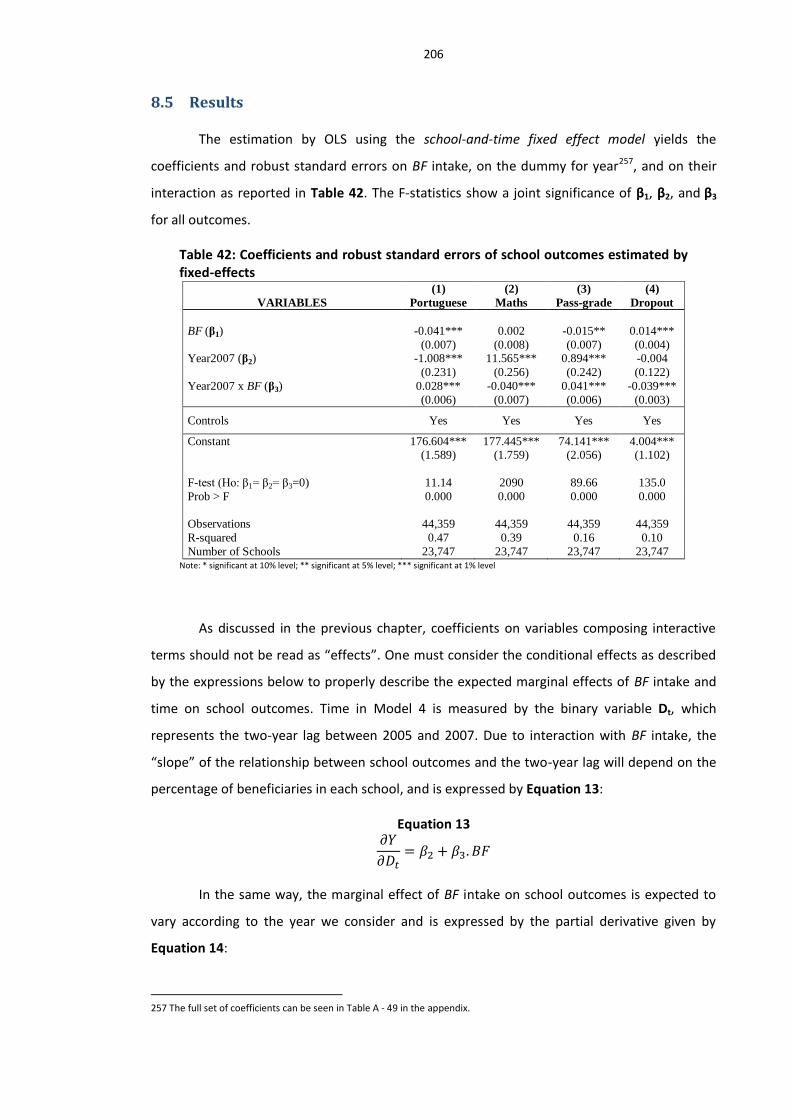
206
8.5 Results
The estimation by OLS using the school-and-time fixed effect model yields the
coefficients and robust standard errors on BF intake, on the dummy for year257, and on their
interaction as reported in Table 42. The F-statistics show a joint significance of β1, β2, and β3
for all outcomes.
Table 42: Coefficients and robust standard errors of school outcomes estimated by fixed-effects
(1) (2) (3) (4)
VARIABLES Portuguese Maths Pass-grade Dropout
BF (β1) -0.041*** 0.002 -0.015** 0.014***
(0.007) (0.008) (0.007) (0.004) Year2007 (β2) -1.008*** 11.565*** 0.894*** -0.004
(0.231) (0.256) (0.242) (0.122)
Year2007 x BF (β3) 0.028*** -0.040*** 0.041*** -0.039***
(0.006) (0.007) (0.006) (0.003)
Controls Yes Yes Yes Yes
Constant 176.604*** 177.445*** 74.141*** 4.004*** (1.589) (1.759) (2.056) (1.102)
F-test (Ho: β1= β2= β3=0) 11.14 2090 89.66 135.0
Prob > F 0.000 0.000 0.000 0.000
Observations 44,359 44,359 44,359 44,359
R-squared 0.47 0.39 0.16 0.10
Number of Schools 23,747 23,747 23,747 23,747 Note: * significant at 10% level; ** significant at 5% level; *** significant at 1% level
As discussed in the previous chapter, coefficients on variables composing interactive
terms should not be read as “effects”. One must consider the conditional effects as described
by the expressions below to properly describe the expected marginal effects of BF intake and
time on school outcomes. Time in Model 4 is measured by the binary variable Dt, which
represents the two-year lag between 2005 and 2007. Due to interaction with BF intake, the
“slope” of the relationship between school outcomes and the two-year lag will depend on the
percentage of beneficiaries in each school, and is expressed by Equation 13:
Equation 13
In the same way, the marginal effect of BF intake on school outcomes is expected to
vary according to the year we consider and is expressed by the partial derivative given by
Equation 14:
257 The full set of coefficients can be seen in Table A - 49 in the appendix.

207
Equation 14
Equation 13 and Equation 14 can be used to analyse changes in marginal effects
related to BF intake on school outcomes over time. Consider, for instance, the case in which Y
represents test scores in Portuguese in Equation 14. Although that marginal effect is assumed
to be constant across schools, it will be allowed to vary between 2005 and 2007 according to
the coefficient on the dummy Dt (β3). The parameter β1 is, thus, an estimate of the average
effect of BF intake on school test scores for the year 2005 (Dt=0). It estimates by how many
points the mean test score is expected to change on average for each percentage point
increase in the proportion of beneficiaries in a given school in that year. Due to the
“programme placement effect”, schools with higher BF intakes are expected, on average, to
perform worse than schools with lower proportions of BF beneficiaries – a result confirmed by
the negative and significant β1 in Table 42 in the case of Portuguese (-0.041). On average, a 10
p.p. increase in BF intake is associated with a 0.4-point reduction in the school mean test score
in Portuguese in 2005.
The coefficient β3 in Equation 14 comes into effect when the dummy variable for time
is equal to one (Dt=1), which is true when the year is 2007. This means that β3 estimates the
average difference of the BF intake effect between 2005 and 2007. There are three possible
results for β3:
If β3 = 0 → there has been no change in the BF intake effect on test scores between 2005 and 2007.
If β3 > 0 → the negative BF intake effect on test scores has been reduced between 2005 and 2007.
If β3 < 0 → the negative BF intake effect on test scores has increased between 2005 and 2007.
The null hypothesis (Ho) to be tested in the case of test scores is against the
alternative hypothesis (Ha) . The alternative hypothesis predicts a positive change in
test scores associated with BF intake between 2005 and 2007. If H0 is rejected, it implies that
the negative marginal effect of BF intake on Portuguese test scores in 2005 is reduced in 2007
on average by β3 for each percentage point in BF intake. This would mean that between 2005
and 2007, marginal gains in test scores due to BF intake took place, reflecting potential
positive effects of participation in BF. Figure 13 illustrates the linear relationship between test
scores and BF intake in each year in the case β3 > 0 given β1<0.

208
Figure 13: Hypothesis of diminishing marginal effect of BF intake on school outcome (Y)
In order to systematically address the full set of hypothesis to be tested regarding the
different school outcomes, three questions are considered based on Equation 14: (i) Does BF
intake affect the school outcome Y?; (ii) Does BF intake degrade the school outcome Y?; (iii)
Does the effect of BF intake on the school outcome Y improve over time? The last question
holds the central hypothesis of interest, which relates to the potential contribution BF might
make to school outcomes over time. Table 43 describes the hypothesis to be tested for each
school outcome, the statistical test used, the result, and the conclusion based on the
estimated models in Table 42.

209
Table 43: Hypothesis tests for the effects of BF intake on school outcomes School
outcome (Y)
Hypothesis to be tested (Ha)
Ho (Null) Test Results Conclusion
Po
rtu
gues
e
Does BF intake affect test scores in Portuguese?
β1 = β3 = 0 F-test F = 15.98
Prob > F = 0.000
BF intake affects Portuguese test scores
Do test scores decrease with BF intake?
β1 + β3.Dt ≥ 0
One-tail t-tests: i) Dt=0: β1≥0 (t-test) ii) Dt=1: β1 + β3 ≥ 0 (t-test)
i) t = -5.61 Prob.>|t|=0.000 ii) t = -2.47 Prob.>|t|=0.007
i) Test scores decrease for Dt=0 (2005) ii) Test scores decrease for Dt=1 (2007)
Does the effect of BF intake on test scores improve over time?
β3 ≤ 0 One-tail t-test t = 4.44 Prob.>|t|=0.000
The effect of BF intake on test scores improves between 2005 and 2007.
Mat
hem
atic
s
Does BF intake affect test scores in Mathematics?
β1 = β3 = 0 F-test F = 30.37 Prob > F = 0.000
BF intake affects Mathematics test scores
Do test scores decrease with BF intake?
β1 + β3.Dt ≥ 0
One-tail t-tests: i) Dt=0: β1≥0 (t-test) ii) Dt=1: β1 + β3 ≥ 0 (t-test)
i) t = 0.19 Prob.>|t|=0.425 ii) t = -6.36 Prob.>|t|=0.000
i) Test scores do not decrease for Dt=0 (2005) ii) Test scores decrease for Dt=1 (2007)
Does the effect of BF intake on test scores improve over time?
β3 ≤ 0 One-tail t-test t = -5.70
Prob. > |t|=0.999
The effect of BF intake on test scores does not improve between 2005
and 2007.
Pas
s-gr
ade
Does BF intake affect pass-grade rates?
β1 = β3 = 0 F-test F = 29.78 Prob > F = 0.000
BF intake affects pass-grade rates
Do pass-grade rates decrease with BF intake?
β1 + β3.Dt ≥ 0
One-tail t-tests: i) Dt=0: β1≥0 (t-test) ii) Dt=1: β1 + β3 ≥ 0 (t-test)
i) t = -2.01 Prob.>|t|=0.022 ii) t = 4.99 Prob.>|t|=0.999
i) Pass-grade rates decrease for Dt=0 (2005)
ii) Pass-grade rates do not decrease for Dt=1(2007)
Does the effect of BF intake on pass-grade rate
improve over time? β3 ≤ 0 One-tail t-test
t = 6.72
Prob. > |t|=0.000
The effect of BF intake on pass-grade rates
improves between 2005 and 2007.
Dro
po
ut
Does BF intake affect dropout rates?
β1 = β3 = 0 F-test F = 98.62 Prob > F = 0.000
BF intake affects dropout rates
Do dropout rates increase with BF intake?
β1 + β3.Dt ≤ 0
One-tail t-tests: i) Dt = 0: β1 ≤ 0 (t-test) ii) Dt = 1: β1 + β3 ≤ 0 (t-test)
i) t = 3.49 Prob.>|t|=0.000 ii) t = -8.15 Prob.>|t|=1.000
i) Dropout rates increase for Dt=0(2005)
ii) Dropout rates do not increase for Dt=1(2007)
Does the effect of BF intake on dropout rate
improve over time? β3 ≥ 0 One-tail t-test
t = -12.39
Prob. > |t|=0.000
The effect of BF intake on dropout rates
improves between 2005 and 2007.

210
Based on the results in Table 43, it can be concluded that BF intake influences all four
of the school outcomes analysed. In 2005, all school outcomes, except Mathematics,
deteriorate with BF intake. However, as assessed by the third hypothesis, the negative impact
of BF intake on school outcomes is reduced between 2005 and 2007 for test scores in
Portuguese, pass-grade rates, and dropout rates. The magnitude of the marginal effects of BF
intake on school outcomes in both years is given in Table 44, nationally and by region258.
Table 44: Marginal Effect of BF intake on school outcomes by region estimated for 2005 and 2007
Note: * significant at 10% level; ** significant at 5% level; *** significant at 1% level
Although the point estimates in Table 44 give us the full picture of the marginal effect
of BF intake in each year259, a graphical representation of Equation 14 helps to depict not only
the point estimates, but also their confidence intervals and the changes that occurred between
2005 and 2007. Figure 14 shows the average national marginal effects of BF intake on school
outcomes in each year of the panel. Since the confidence intervals do not overlap for any of
the outcomes, the marginal effects are all statistically different between 2005 and 2007.
Figure 14: Marginal effects of BF intake on school outcomes by year (NATIONAL)
258 The estimates by region derive from restricting the sample of schools to each region before regressing Model 4.
259 Because the marginal effect of BF intake varies only with the dummy Dt, there are only two possible values to be estimated.
2005 2007 2005 2007 2005 2007 2005 2007 2005 2007 2005 2007
Portuguese -0.041*** -0.013** -0.043** 0.015 -0.015 -0.005 -0.093*** -0.018 -0.068*** 0.000 -0.045*** -0.028**
Maths 0.002 -0.038*** -0.016 -0.009 0.005 -0.002 -0.040 -0.024 -0.027 -0.022 0.000 -0.055***
Dropout rate 0.014*** -0.025*** 0.011 -0.017* 0.016 -0.019** 0.020 -0.020 0.002 -0.014*** 0.009** -0.006**
Pass-grade rate -0.015** 0.026*** -0.054*** 0.021 -0.020 0.020* -0.040* 0.016 0.021 0.051*** -0.045*** 0.010
Region
BrazilSchool Outcome North Northeast Central-West Southeast South
-.05
0
.05
-.05
0
.05
2005 2007 2005 2007
Math Port
Pass-grade Dropout
dY/dBF 95% c.i.
Year
Graphs by outcome

211
For test scores in Portuguese, although the marginal effect is still negative in 2007, it
clearly diminishes in absolute terms in relation to 2005 results, suggesting that, on average,
schools with higher percentages of participants in BF improved more than schools with lower
BF participation rates between 2005 and 2007. That improvement occurred despite schools’
time invariant characteristics and despite those factors related to school composition and
school resources controlled for (as listed in Table A - 49). This trend is even stronger for the
North, Central-West, and Southeast regions (see Figure A- 2). In the South, although the point
estimate seems to improve in Table 44, the marginal effects are not statistically different from
each other. In the Northeast, neither in 2005 nor in 2007 is the BF marginal effect statistically
distinguishable from zero260. These results suggest a potential benefit to schools’ test scores in
Portuguese due to participation in BF nationally and in three of the five regions.
The estimated change in the marginal effect of BF intake on pass-grade rates also
shows improvements between 2005 and 2007, becoming positive at the national level in 2007.
While in 2005 a 10 p.p. increase in BF intake was associated with a 0.15 p.p. decrease in pass-
grade rates, in 2007 the same variation in BF intake is associated with a 0.26 p.p. increase in
pass-grade rates. The same trend of improvement is statistically distinguishable (at the 5%
level) in the North and South regions, and is also noted in the other regions, although with
more statistical ambiguity (see Figure A- 3). Schools also present lower dropout rates
nationally by percentage point of BF intake in 2007, as compared to 2005. While in 2005 10
p.p. more beneficiaries are associated with an increase in dropout rates by 0.14 p.p., in 2007
the same variation in BF intake is associated with a decrease in dropout rates by 0.25 p.p. All
regions perceive improvements by proportion of beneficiaries, although it is only in the
Northeast, Southeast, and South that improvements are statistically distinguishable261 from
zero, as shown in Figure A- 4.
With test scores in Mathematics, there is a different picture, as the national average
marginal effect becomes negative in 2007 after being not different from zero in 2005. Looking
at the results by region (see Figure A- 5), one sees no significant marginal effect for BF intake,
except in the South in 2007. Technically, in analysing by region, no change in the BF intake
marginal effect is detected between 2005 and 2007, since all confidence intervals overlap. The
more plausible conclusion is that no improvement took place by region related to BF intake.
The national result, however, may suggest that the relationship between the share of
260 The regression coefficients for the Northeast in the school fixed-effects model (β1 β2 and β3) are jointly statistically
insignificant. This means that schools in that region did not observe any change in the mean test score in Portuguese between
2005 and 2007 due either to time trends or to variations in BF intake.
261 The South at 5% and the Northeast and Southeast at 10%.

212
beneficiaries in a school and poor performance in Mathematics is getting stronger over time,
instead of attenuating as a potential consequence of participation in Bolsa Família.
Nevertheless, some caution is necessary in this interpretation, because despite the control
factors in estimating Model 4, a large and significant increase in Mathematics test scores took
place between those years, as attested by the coefficient β2 for Mathematics in Table 42. By
plotting the marginal effect of the dummy variable for the year by the proportion of
beneficiaries (Equation 13), we can see how the effect of the two-year lag affects school
outcomes differently according to the value of BF intake. We can also clearly see what happens
with Mathematics (Figure 15).
Figure 15: Marginal effects of time on school outcomes by level of BF intake (NATIONAL)
Figure 15 shows the marginal effects of time for different values of BF intake for each
of the four school outcomes. In fact, the plotted marginal effects of Dt on school outcomes are
the estimated differences in those school outcomes between 2005 and 2007 at different
values of BF intake. For Portuguese test scores, pass-grade, and dropout rates the marginal
effect translates into better results for higher levels of BF intake, confirming the
results previously discussed. In the case of Mathematics, it can be seen that the two-year lag
has a positive and significant effect on test scores for all values of BF intake. However, those
schools with lower proportions of beneficiaries seem to have gained more of whatever
explains the general improvement of test scores in Mathematics between those two years. It is
-4-3
-2-1
0
60 20 40 60 80 100
% of BF
dDropout/dDt 95% c.i. stat.signf.
Dropout
02
46
1000 20 40 60 80 100
% of BF
dPass/dDt 95% c.i. stat.signf.
Pass-grade
-10
12
3
28 480 20 40 60 80 100
% of BF
dPort/dDt 95% c.i. stat.signf.
Portuguese
68
10
12
0 20 40 60 80 100% of BF
dMath/dDt 95% c.i. stat.signf.
Maths

213
even possible that the factor(s) causing the improvement of test scores for low BF intake
schools are different from those explaining the improvement detected for high BF intake
schools. For instance, if special programmes focused on Mathematics teaching had been
introduced, reaching more advantaged schools between those years, it would be possible to
observe a faster improvement for schools at the bottom of BF intake distribution, while those
at the top of the distribution might lag behind despite the possible gains accrued by poor
children from participating in BF. In sum, the negative marginal effect of BF intake estimated
for test scores in Mathematics in 2007 reflects the larger improvement obtained by schools
from the lower ranks of BF intake, rather than the decline of the results of those holding larger
shares of beneficiaries, since the latter also observed improvements in test scores. The
problem is that in the case of Mathematics, the possible gains from BF are probably
overshadowed by the gains obtained by more advantaged schools during that period. Without
knowing what factor explains the gains over time for low BF intake schools, it is not possible to
include it in the model in order to purge those effects from the time effect captured by the
dummy Dt262.
8.6 Conclusions and Limitations
The initial analysis of the two years of panel data in this chapter showed that school
outcomes improved between 2005 and 2007, with increasing gains for schools at the top of
the BF intake distribution. As a result, the performance gap between schools in the first and
fifth quintiles of BF intake diminished over those years. At first glance, these changes may
suggest a positive contribution of BF to school outcomes. However, it was also shown that
school composition in terms of student and household characteristics, as well as school
resources, changed between 2005 and 2007 across levels of BF intake. Those are influential
factors on school outcomes, and the observed changes were shown to benefit schools in the
top quintiles of BF intake. In addition, schools also changed in terms of their share of
beneficiaries between those years, suggesting that the observed improvements at the top of
the BF intake distribution might be due to transitions of schools to different groups of BF
intake. The different cohorts of pupils (and beneficiaries) in the two national exams, and the
transitions of schools across groups of BF intake, might give the impression that larger shares
262 One of the possible explanations for the improvement in test scores in Mathematics in 2007 raised by the Ministry of
Education is the Mathematical Olympiad created nationally in 2004 and first run in 2005. In 2005, it reached 31,031 public schools
in 93.3% of municipalities in Brazil and in 2007 a total of 38,450 schools took part in the competition covering 98.1% of
municipalities in Brazil. By the time this research was finished, the information on which schools took part in each year in the
Olympiad was not made available. Therefore, it was not possible to test if the Mathematical Olympiad was acting as an omitted
variable for the national exam’s results in Mathematics.

214
of BF participation, in itself, was causing the observed improvements in school outcomes
across years. A school-and-time fixed effects model tested the hypothesis that BF participation
holds a share in explaining the observed improvements in school outcomes (despite changes in
school composition, resources, and proportion of beneficiaries).
The estimated school-and-time fixed effects model (Model 4) manages to control for a
set of school compositional characteristics and resources over time, as well as for time
invariant school characteristics and school invariant trends over time. By avoiding several
potential confounding factors, the panel analysis allows us to capture changes in the marginal
effect of BF intake across time. The results show that, although the proportion of beneficiaries
has a deteriorating effect on school outcomes in 2005 (except in Mathematics), that effect is
reduced between 2005 and 2007 for test scores in Portuguese and becomes positive for pass-
grade and dropout rates. The two-year period positively affects schools at higher levels of BF
participation more than those at the bottom of the BF intake distribution for those school
outcomes, a trend also observed at the regional level. In Mathematics, however, results are
blurred by unknown factors that somehow positively affected low BF intake schools more than
high BF intake schools. Despite this, the overall results support the idea that marginal gains
associated with BF intake over time potentially reflect direct contributions of BF to school
outcomes.
However, some caveats remain. First, Model 4 does not allow for a clear-cut pre/post
policy change assessment, since Prova Brasil started in 2005 when BF had already been in
place for almost two years, amounting to eight million families. The panel data makes use of
an alternative post-programme implementation baseline that allows measures of change in
relation to 2005. Therefore, the estimated effects are relative to 2005 and do not translate the
full picture of how BF might be influencing school outcomes over time. Second, the coefficient
estimated on the interaction term (β3) might be translating other policies targeted towards
schools or families in deprived areas coinciding with BF targeted families. In this case, the
improvements related to the marginal effect of BF intake might not be a result of BF itself, but
of other educational policies driven towards high BF intake school communities. Nevertheless,
given the highly decentralised political system in Brazil, it is unlikely that local initiatives would
create a national effect, if not part of a nationally-induced programme. By 2007, no nation-
wide policy was in place to add extra resources to schools based on the level of participation in
BF. The likelihood is that any marginal gain related to BF intake is, in fact, an effect of the cash
transfer and its conditionalities. Third, the lack of information on characteristics related to
participation in BF, such as the value of the cash transfer and length of time of participation for
215
each family in both years in the panel, prevents any conclusion about the relevance of these
factors to the improvements estimated by the BF intake marginal effect. However, the
consistency between the results found in the panel analysis with those arising from the cross-
sectional analysis developed in the previous chapter strongly suggests that the improvements
in school outcomes between 2005 and 2007 are, in fact, a direct contribution of the benefits
BF brings to the educational opportunities of children of low-income families.

216
Chapter 9. Main Findings
9.1 Introduction
The investigation of whether Bolsa Família makes any positive contribution to the
educational outcomes of economically disadvantaged children in Brazil followed the analysis of
three empirical questions that can be summarised as follows:
What can explain the achievement gap between BF beneficiaries and non-
beneficiaries in the national exam?
Do time of exposure and per capita cash paid to families in BF positively
influence school results and reduce the achievement gap between high-BF-
intake schools and low-BF-intake schools?
Did schools observe any improvement in outcomes between 2005 and 2007
that can be associated with the level of BF participation in each school?
In pursuing answers to these questions I first explored some of the direct
consequences of poverty on children’s opportunities and outcomes as reported in the
literature, particularly outcomes in education. Several of the mechanisms operating through or
moderated by family income discussed in the literature suggest that many of the current
attempts to address unequal educational achievements and to promote the education for
children of low-income families by merely addressing intra-school factors are likely to fail. How
income is distributed in society is at least as important as the way society allocates educational
resources to different social groups to promote equal educational opportunities. In this sense,
some equality of outcomes is required as a base upon which equality of opportunities can be
made effective (Esping-Andersen, 2009). Parent’s incomes are, in many respects, the starting
point for children’s present and future outcomes, and schools cannot compensate for many
socially inherited conditions. The playing field in the present is simply not level for millions of
children, even when schools are available. It is at this point that the human capital theory
collapses. It works for children and youths who are able to benefit from what schools have to
offer. But benefitting from schools requires some social minimums that many children may fall
short of. This recognition invites a rethinking of the human capital paradigm. Policy-makers
should start by asking a different question: what reduction of child poverty can do for schools
and education in the present? This question presents a new challenge to policy-makers in
integrating socio-educational policies to tackle socio-educational inequalities. Perhaps income
transfer is not the sole response, but it is a necessary one.

217
The theoretical models discussed in this thesis explaining the relationship between
family income and children’s outcomes allow us to envisage at least four main influences
relevant to educational outcomes: (i) parents’ capacity to invest time and money in children’s
education; (ii) social experiences mediating and moulding children’s values, behaviours,
choices, and expectations that affect their development; (iii) parents’ capacity to cope with
psychological distresses that can affect their ability to support and maintain a healthy
environment for children; and (iv) school functioning for economically disadvantaged children.
Attacking income inequality and poverty amongst families is not only relevant to directly
addressing parents’ capacities to provide a better home and social environment for children’s
education, but also might be very important in resetting the school functioning for the children
from the most disadvantaged families.
Empirical studies developed over the last 40 years in the US (reviewed in chapter two)
show that cash transfer programmes may have significant effects on the educational outcomes
of children of low-income families. Positive impacts of welfare and anti-poverty programmes
were found in respect to enrolment and graduation in high school, attendance rates,
comportment, academic achievement, and years of schooling. Based on those studies, I
identify some general aspects which policy-makers should pay attention to for an effective
cash transfer policies. First, early interventions are vital in mitigating the potential damages to
education, since most evidence recognises that children arrive at school already at very
different levels of readiness to benefit from any learning experience. Moreover, young children
attending lower grades are more likely to benefit from additional income paid to their families
than older children or those in higher grades. This is probably because the youngest are more
dependent on their parents; they have less freedom of choice and are the most affected by
parents’ circumstances in a way that can have an impact on their education. Second, cash
transfer policies must be able to affect families’ permanent income, thereby affecting the
patterns of consumption in the household. Any policy in this respect must avoid irregular,
insufficient, or transient hand-outs that are incapable of affecting household permanent
income. Third, time of exposure to cash transfer programmes is relevant in gauging effects on
educational outcomes, particularly learning (three or more years in most of the studies). This is
consistent with the idea that cash transfer policies must endure so to affect permanent income
and patterns of consumption that can, in turn, change the environment for children. It is also
consistent with the idea that learning outcomes are probably the most difficult and take the
longest to be influenced by cash transfer policies. Fourth, the effect of income increases on
educational outcomes also varies with the level of poverty. It turns out that the poorer the

218
family is, the more relevant the impacts of the cash transfer for children. The cash value
relative to the household per capita income is a key factor in explaining the potential effect
cash transfers may have on children’s educational outcomes. These are general findings that
should guide policy-makers in designing cash transfer policies in which children’s educational
outcomes are amongst the main objectives.
I also discussed in this thesis the role conditional cash transfer programmes may have
in mitigating poverty’s effects on children’s educational outcomes in developing countries. A
significant amount of research has demonstrated the operational efficacy of these
programmes in targeting the poor and in producing expected social outcomes, such as
alleviating poverty in the short term, increasing health and nutritional conditions for children,
and assuring higher levels of enrolment and attendance in school. If for no other reason, these
results alone could justify public investments in CCTs. However, human capital accumulation is
at the core of the long-term objectives, as stated in most CCT blueprints. As argued in chapter
three, human capital accumulation can only be justified if CCTs can make any positive
contribution to the learning outcomes, promotion, and completion rates of beneficiary
children. So far, research on CCTs has failed to produce any convincing evidence of these
effects, particularly the first, for which null or even negative effects have been reported in the
literature. Nevertheless, this absence of results contrasts with the large collection of social
experiments and longitudinal studies reviewed in chapter two showing the effects of welfare
and anti-poverty programmes on the educational outcomes of beneficiary children. Amongst
the many possible reasons that researchers have failed in detecting CCTs’ effects on learning
outcomes, two stand out. First, the timeframe in which studies on CCTs have been carried out
tend to be shorter than the timeframe in which research in the US was able to detect many of
the educational effects, particularly learning outcomes. Second, the value of cash paid by CCTs
to families has, so far, found very little space in the analysis of CCT effects on education.
Working with these two testable hypotheses, I come to the core of the empirical analysis in
this thesis: the investigation of whether Bolsa Família in Brazil is contributing to achievement
in standardised test scores in Portuguese Language and Mathematics of fourth grade students,
as well as to pass-grade, and dropout rates.
Bolsa Família (and its predecessor Bolsa Escola) has been recognised in the literature
as a main contributor to the staggering reduction in poverty and inequality in Brazil since the
early 2000s. The question remaining is whether by reducing poverty and inequality in the short
term, BF can also be an effective policy in creating human capital amongst the poor in the long
term. The condition for that to occur relies on the potential effects BF might have on

219
promotion and completion rates, which, in turn, depend on the possibility that beneficiaries
will experience improvements in learning outcomes, as described in the socio-educational
framework proposed in chapter four. Evidence in the literature so far has shown clear positive
effects on increasing school enrolment and attendance, and on reducing dropout rates. These
are immediate outcomes derived from the institutional rules requiring families to enrol their
children and to ensure that they attend school at a minimum rate per month. The more
challenging effect of improvements in learning outcomes had not been studied yet on a
national scale in Brazil, due in part to the lack of national test score data at the school level
until very recently. When studies of CCT programmes in other countries have tried to evaluate
effects on test scores or any other measure of learning outcomes, no effect was detected
either. That key missing link is at the core of analysis in this thesis.
I have found evidence which strongly suggests that, in the case of BF, the effects on
learning outcomes do exist, as do effects on pass-grade and dropout rates. I have found this by
exploring, in tandem, the two conditions so far absent from research on this topic: time of
exposure and cash value paid to families. In the next sections I summarise the main results and
limitations of the empirical analysis.
9.2 The achievement gap between beneficiaries and non-beneficiaries
In the first part of the empirical analysis, I examined the achievement gap between
beneficiaries and non-beneficiaries in Prova Brasil 2005 and how differences in terms of
individual, household, and school characteristics explain that gap. My analysis shows that, on
average, beneficiaries perform less well than non-beneficiaries by 16 points in Mathematics
and by 20 points in Portuguese Language. Those differences are equivalent to two-thirds and
three-quarters of one cognitive level, respectively, or 0.4 and 0.5 s.d. from the national mean.
These gaps can be translated into months of schooling, as equivalent to five and seven months
respectively. The achievement gap between beneficiaries and non-beneficiaries increases with
income inequality, as measured by a proxy variable (durable goods index) showing that family
income is associated with achievement in test scores in Brazil. The extension of that
association was further examined in chapter six by exploring a set of individual, household,
and school characteristics that may intervene with children’s educational outcomes, and that
are also correlated with the condition of being a beneficiary of BF.
The analysis in chapter six shows that beneficiaries are at a disadvantage, not only in
terms of family income (which is an eligibility criterion to take part in BF). In addition to living

220
in more crowded and materially poorer households, beneficiaries are more likely to be
engaged in domestic or paid work and receive less encouragement from parents for school
related activities (parents who are generally less educated as well). Beneficiaries are more
prevalent amongst those students who did not attend pre-school and have experienced grade
failure and dropouts in past years. These students feel more marginalised in the classroom
than non-beneficiaries and tend to study in less well-resourced schools, either in terms of
infrastructure or teacher quality. Despite all this, beneficiaries share with non-beneficiaries the
same expectations regarding achieving secondary education. The multiple disadvantages of
beneficiaries are significant and explain part of the achievement gap mentioned above.
Once specific characteristics of students, families, and schools are taken into account,
the analysis of test score differences in Portuguese Language according to BF participation
reveals the relative weight of those factors in explaining the achievement gap. Students’ past
and present experience in school and students’ time allocation when not at school are major
contributors, explaining 28% of the achievement gap between beneficiaries and non-
beneficiaries (after accounting for gender and race). A difference as large as 28 points in
Portuguese Language (equivalent to one year of schooling) is estimated to derive from not
attending pre-school, failing any grade in previous years, and experiencing a lack of attention
from teachers when attending the fourth grade. Another difference of 20 points is attributed
to involvement in domestic and any form of paid job outside the home. By not being able to do
homework, students lose another seven points in test scores, on average. Those losing in all
these respects are more likely to be beneficiaries.
Household characteristics explain another 15% of the gap between beneficiaries and
non-beneficiaries. The material environment at home seems to be even more relevant than
parents’ characteristics, such as education and participation in school meetings. For instance, a
child who lives in a house with bathroom and bedroom, with access to running water and
electricity, has, on average, a test score higher by 28 points in Portuguese Language (one year
of schooling) compared to a child whose household has none of these facilities. Parents with
post-primary education is associated with no more than an additional eight points in test
scores, while parental participation in school meetings is associated with an additional four
points. Still significant, but less influential than the previous factors, is the family structure in
terms of the size and presence of both parents in the household. Together, these factors are
associated with seven points more on the average test score in Portuguese. These results show
the importance of material poverty to students’ performance at school relative to other
aspects within the household context.

221
Students’ individual characteristics, together with household characteristics, explain
44% of the existing gap between beneficiaries and non-beneficiaries in Portuguese tests
scores. By introducing school-related factors (infrastructure, student-teacher ratio, teachers’
education, and practice of assigning homework) the additional proportion to the explained gap
is just 4.5%. These results suggest that the achievement gap is, in large part, due to conditions
not related to school supplies or to teachers’ related variables. Instead, it is what happens (or
does not happen) at home and what children bring (or do not bring) to school that makes the
bulk of the difference. However, I do not disregard the influence of schools on children’s
outcomes. What students experience at school in the years prior to and during the fourth
grade is relevant, as shown by the large share of the achievement gap explained by the set of
variables that I call “students’ school history” (pre-school attendance, grade failure in previous
years, and feeling of being neglected in the classroom). Nevertheless, socioeconomic
disadvantages seem to play a major role in explaining why BF beneficiaries lag behind in school
achievement compared to non-beneficiaries. By focusing on socioeconomically disadvantaged
families, BF is expected to mitigate some of the harmful effects of poverty on the educational
opportunities and outcomes of children of low-income families, and to contribute to reducing
the achievement gap hitherto discussed.
9.3 The influence of Bolsa Família on school outcomes
In the second part of the empirical analysis I focused on investigating the central
hypothesis of this thesis: that time of participation in Bolsa Família (BF) and the per capita cash
paid to families are central variables influencing the potential effect of BF on school results for
beneficiary children (test scores, pass-grade, and dropout rates). Using data from Prova Brasil
2007, I first explored the differences between schools in terms of composition, resources, and
outcomes, asking whether schools’ results are associated with the level of BF intake, with the
mean time of participation in the programme, and with the cash value transferred to families.
The distribution of school resources and outcomes by level of BF intake is clearly
biased against schools holding large shares of beneficiaries. Once participation in BF is
considered a proxy variable for poverty incidence by school, it can be said that school
conditions (and outcomes) deteriorate as the incidence of poverty increases. I have referred to
this as a characteristic of a regressive education system, in which the more disadvantaged the
socioeconomic context of families, the poorer resourced the schools are for their children. The
consequence of both high concentration of poor children and less well-resourced school
environment is low performance in all four indicators analysed in this thesis (test scores in

222
Portuguese and Mathematics, pas-grade, and dropout rates). An achievement gap of one
cognitive level (or one year of schooling) exists between schools in the first quintile (0% to
20%) and those in the fifth quintile (80% to 100%) of BF intake. Dropout rates are, on average,
three times higher and pass-grade rates 9 p.p. lower for schools in the fifth quintile compared
to schools in the first quintile. At the same time, the correlations between the mean school
outcomes and BF households’ per capita incomes suggest that changes in the severity of
poverty amongst poor families can affect the overall school result. Can those gaps be different
if families take part in BF for a period of time that changes poverty conditions so as to benefit
children’s school outcomes?
The analysis in chapter seven shows that BF factors at the school level (intake, mean
time of participation, and mean per capita cash) interact in predicting changes in school
outcomes. All four outcomes at the school level are functions of those three BF factors, even
after controlling for several household and school characteristics. An “average school” in terms
of time of participation (two and a half years) and mean per capita cash (R$ 17.2) has an
estimated improvement due to BF participation on both dropout and pass-grade rates of 0.2
and 0.1 p.p. respectively for each 10 p.p. increase in BF intake. This means that between two
schools with same composition (except the level of BF participation), the same school
resources, and located in the same region, the one with high proportion of beneficiaries will
perform better in terms of pass-grade and dropout rates263. This evidence suggests a
contribution of BF to two school outcomes for which the poorest students are clearly at a
disadvantage. What about test scores — the missing link?
The analysis shows that although schools with higher proportions of beneficiaries tend
to perform worse on the national exam, that negative effect reduces as average time of
participation and average per capita cash increases. Schools in which families have
participated in BF for a longer period of time or in which families have been paid a higher per
capita benefit, beneficiary children perform better on the national exam, since their presence
in the school degrades the mean test score by a lower marginal rate. In addition, the variables
Time and Cash were found to have substitute effects on test scores; although the results
strongly suggest that both Time and Cash have positive effects on test scores for beneficiaries,
these effects interfere with one another in opposite directions. In other words, as per capita
cash value increases, beneficiaries’ performance improves, but the positive contribution of
time of participation to their performance diminishes. In the same way, as time of
participation increases, beneficiaries’ performance improves, but the positive contribution of 263 A positive marginal effect of BF intake is also found for the Northeast region.

223
per capita cash to their performance diminishes. The net effect, however, is a gain in test
scores for beneficiaries due to both time of participation in the programmes and per capita
cash transferred to families.
Due to the substitute effect, the gains promoted by Time and Cash on test scores are
limited by one another. I estimated the threshold for increases in the variable Time beyond
which the positive contribution of Cash to test scores is completely annulled. For time of
participation beyond three years, increases in the mean per capita cash of families have no
extra benefit for the average performance of beneficiary children on tests scores. In the same
way, a threshold exists for Cash beyond which increases in time of participation brings no
additional contribution to test scores. That threshold is around R$ 25 per capita. In 2007, the
large majority of schools were far from those limits, meaning that the large majority of
beneficiaries could still benefit from either more time in the programme or higher cash
transfers to their families.
So far, the conclusion that BF contributes to the school mean test score through the
two factors analysed in this thesis (Time and Cash) does not tell us the practical significance of
that contribution. To determine this significance, I used the interactive model to estimate the
predicted gap between schools at extreme points of the distribution of BF intake (0% and
100%) when time of participation varies between one and four years264. A reduction in that
gap of 14.5 points in Portuguese Language test scores (76%), or 0.85 s.d., was estimated when
time of participation increased from one to four years. In schools where all children are
beneficiaries, an increase of 10.6 points (0.62 s.d.) was estimated when exposure to the
programme increased by three years. It was also shown that the mean test score is affected by
time of participation only in schools where the proportion of beneficiaries is above 45%. These
results show that even small marginal effects can be translated into significant changes of
mean results at the school level.
In order to estimate the direct marginal effects of Time and Cash on school outcomes, I
used a subsample of schools from the fifth quintile of BF intake (80% to 100%). For this group,
the proportion of beneficiaries can be considered invariant across schools in terms of its effect
on school outcomes. Pass-grade rates were estimated to improve by 0.6 p.p. for a one real
increase in the mean per capita cash amount paid to families. This effect is invariant with time
of participation in the programme, suggesting that an equivalent effect on pass-grade rates
can be expected across schools, independent of the mean time of exposure to BF. On the
264 The per capita cash value was fixed at the fifth percentile (R$ 12.20) for these estimates.

224
other hand, time of participation has no effect on pass-grade rates for this group of schools.
Dropout rate is expected to fall by 0.6 p.p. for each additional 10 months of participation in BF.
Differences in the mean per capita cash paid to families do not matter with respect to dropout
rates for the schools in the fifth quintile of BF intake. This result suggests that above the
minimum per capita cash value observed in the subsample (R$ 11.50), no reduction in dropout
is expected to occur as a result of any increase in per capita cash.
Regarding effects on test scores, only Portuguese is affected by BF factors in schools
of the fifth quintile, not Mathematics265. On average, until 27 months of participation, results
in Portuguese Language benefit from cash increases by a rate between 0.4 and 1.7 points per
real increased. The magnitude of this seemingly tiny marginal effect can be seen in the
estimated gain in test scores of 0.34 s.d. due to an increase of one s.d. in the per capita cash
(R$ 2.16)266. The results show that for schools of the fifth quintile of BF intake, after two years
in the programme, no significant extra gain will be observed in test scores if per capita cash is
augmented. Any improvement in test scores for the poorest group of schools seems to come
from the initial incentives provided by the programme. Differences in time of participation did
not turn out to be positively associated with test scores for this group and, in fact, the results
suggest that Time has a “discount effect” on any gains obtained from cash transfers for values
above R$ 19.40.
These results strongly suggest that BF factors (intake, time of participation, and per
capita cash) matter for school outcomes, but some caveats must be borne in mind. The
relevance of BF effects varies across regions and probably across schools. However, the
estimates reported in this study assume homogeneous effects across schools. Therefore, the
results represent national (or regional) average effects that might differ in more specific
contexts. The results are also estimated for schools as a whole, not for the group of
beneficiaries in particular. As such, the estimated effects reported can be considered average
treatment effects (ATE), that is, what is expected to happen, for instance, with schools’ mean
test scores not with beneficiaries’ mean test scores in schools. The estimated effects would
probably be higher if estimated for beneficiaries only [average treatment on the treated effect
(ATTE)]; however, this was not possible with the available data. Finally, the validity of the
results depends on the ability of the conditional mean independence assumption to hold up. In
other words, validity depends on the assumption that schools used in the analysis are
265 Although the estimated coefficients for Mathematics had the same sign as those for Portuguese Language, showing the same
trend, they were not statistically significant; therefore, no conclusion is possible with respect to BF influence on Mathematics.
266 When increased at the very beginning of participation in BF.

225
comparable once relevant differences are accounted for in the regression model. Schools are
considered equivalent, on average, with respect to all characteristics that could affect
outcomes and at the same time be correlated with BF factors whose effects are analysed using
cross-sectional data. This last limitation (the comparability between schools) was addressed in
a more robust analysis when I moved from cross-sectional to panel data analysis, as described
next.
In chapter eight I took a step forward to circumvent the limitation imposed by the
cross-sectional analysis by using two years of panel data (2005-2007) to estimate a school-and-
time fixed effects model and to test the hypothesis of a positive change in school performance
between those two years due to participation in BF. The initial analysis shows that the
unadjusted school outcomes improved between 2005 and 2007, with those schools at the top
of the BF intake distribution observing higher gains. As a consequence, the performance gap
between schools in the first and fifth quintiles of BF intake diminished over the two years.
However, school composition and resources also changed between those years, benefiting
those schools with high levels of BF intake proportionally more. This is a positive result in itself,
since the regressive feature of the education system mentioned earlier seems to be reversing;
school resources, for instance, are improving more in schools with high proportions of
beneficiaries. Therefore, the changes in resources and composition, inclusive in terms of BF
intake, might be the driving force behind the improvements in school outcomes for schools on
the top of BF intake distribution.
The estimation of a school-and-time fixed effects model allowed me to control for both
time invariant school characteristics and for trends over time that were invariant across
schools. In addition, a set of controls for school composition and resources were included in
the model to account for possible school characteristics that might change across time and
across schools. The panel analysis allowed the exam of how BF intake affects school outcomes
and, more importantly, whether that effect was changing over time as a potential result of
direct benefits from participation in BF. The results showed that BF intake influences all four
school outcomes analysed. More importantly, the negative impact of BF intake on school
outcomes was found to be diminishing between 2005 and 2007 for test scores in Portuguese
Language, and became positive for pass-grade and dropout rates.
On average schools with higher proportions of beneficiaries improved more than
schools with lower levels of BF participation. In Portuguese, the negative effect of 10 p.p. more
beneficiaries in a school changed from -0.4 points on average to -0.1 between 2005 and 2007,
a 75% reduction. The 10 p.p. more in BF intake was associated in 2005 with 0.15 p.p. decrease

226
in pass-grade rates, while in 2007 it was associated with a 0.26 p.p. increase; for dropout rates
that change was from a 0.14 p.p. increase in 2005 to a 0.25 decrease in 2007 for each
additional 10 p.p. in BF intake. The results differ across regions. An anomalous result was
found in Mathematics, for which the effect of BF intake does not improve between 2005 and
2007, but instead becomes negative after being null in 2005. A possible explanation could be
found by looking at how the effect of the two-year period affected test scores in Mathematics
across different values of BF intake. It was shown that schools with high BF intakes improved
between 2005 and 2007, although less than schools with low BF intakes. The hypothesis raised
is that an omitted variable (possibly the National Mathematical Olympiad that started in 2005)
benefitted schools at the bottom of the BF intake distribution more than schools at the top of
the distribution. It is even possible that the reasons for the improvements observed for schools
with proportionally fewer beneficiaries is different from those explaining improvements in
schools with proportionally more beneficiaries. In this case, any possible gain from BF is
probably overshadowed by those obtained by more advantaged schools. Apart from that
anomaly, the results in general show marginal gains associated with BF intake over time, which
potentially reflect direct contributions of BF to school outcomes.
Again, some caveats must be borne in mind. The panel analysis does not account for a
pre/post policy change assessment; all changes are measured in relation to 2005, one year
after Bolsa Família had started and four years after Bolsa Escola had been launched. Second,
the positive changes observed in the marginal effect of BF intake might still be due to the
overlapping of policies other than BF with schools or families assisted by BF. Nevertheless, that
possibility is unlikely unless it is part of a national policy whose targeting mechanism was
somehow connected to participation in BF and that could affect educational results nationally.
There is no evidence that such a policy took place between those years. Finally, I could not test
the two key variables (time of participation and per capita cash) in the panel analysis since
these variables were not available for 2005. Nevertheless, the consistency of the results
related to the marginal effect of BF intake between the cross-sectional and panel analyses
strongly suggests that at least part of the improvements in school outcomes observed
between 2005 and 2007 is a direct contribution of BF to the educational outcomes of
economically disadvantaged children in Brazil.
Several policy implications can be considered from this set of findings, and several
areas for further research can be identified, which I refer to in the next sections.

227
9.4 Policy implications
In addition to the policy recommendations for an effective cash transfer policy to
achieve educational objectives mentioned in section 9.1, this thesis adds some other aspects
to be considered by policy-makers in the Brazilian context. First, there is an urgent need to
address inequality in standards of education supply in Brazil, as evidenced by the impoverished
educational conditions of schools with high proportions of BF beneficiaries. By extension, BF
participation by school can be used as a proxy for poverty incidence in schools and to target
educational policies focused on improving equity in education systems. Second, given the
major influence of pre-school participation on children’s school outcomes and the clear
disadvantage of BF recipient children in attending pre-school, special attention should be given
to BF families in promoting access to pre-school programmes aside from the nutritional and
health care assistance already promoted by the programme. Third, once per capita cash values
seem to make a difference for children’s educational outcomes, cash transfers should be
tailored based not only on the number of children in the family, but also on the level of per
capita poverty and on regional labour market conditions in order to achieve similar relative
effects for children living in different circumstances. Regional adjustments in the benefit by
proxy variables for the opportunity cost of having children engaged only in studying, such as
labour market attractiveness (wage levels), incidence of child labour, and living cost indexes
(e.g. basic food basket costs) are possible criteria to be considered. Fourth, the substitute
effect between time of participation and the value of the benefit implies that the BF cash-
effect on educational outcomes is maximised when families initially start in the programme.
After three years, for instance, no benefit for test scores is expected from increases in cash,
this threshold being lower (two years) for the poorest schools (with high BF intakes). Policy-
makers might consider different readjustment policies based on time of participation and level
of poverty, granting higher rates to the poorest families with a shorter time in the programme.
Fifth, it is also possible that the substitute effect is reset between school cycles267 (from
primary to lower secondary for example), meaning that a higher benefit per child could be
offered once they achieve the fifth grade and the first year of secondary school. This would
work as an incentive to progress towards upper grades268 and potentially maximise impacts on
education outcomes. Sixth, the large majority of schools in 2007 could still benefit from
increases in the value of cash paid to families (99% of the schools) and from families
267 The marginal effect of cash on school outcomes might pick up again after transition to an upper level of education. This
hypothesis should be further investigated.
268 A similar scheme was operating in the first CCT programme in Brazil (Federal District 1995) as a savings account that
beneficiaries could access after completing secondary school.

228
continuing for longer periods in the programme (90% of schools). Increases in the value of the
benefit occurred on several occasions since 2007269 and, based on the results of this thesis,
probably contributed to improvements in educational outcomes in the large majority of
schools.
These are some aspects that might be considered by policy-makers once attention is
paid to the educational contributions of BF in Brazil. Nevertheless, given the multipurpose
characteristics and large-scale coverage of the programme, policy-makers must consider how
adjustments in the benefit scheme or in other aspects of the policy are communicated to the
population, how they may affect families’ perceptions and reactions to the programme, and
how eventual changes may affect the programme’s objectives other than education. This
makes the task of adjusting BF a real challenge for policy-makers. However, greater progress
for children’s educational outcomes may rely on that task.
9.5 Final remarks and indications for further research
Throughout this thesis I have argued that the impact of poverty on children’s
educational opportunities can be, to some extent, mitigated by welfare and anti-poverty
programmes. The analysis of the BF case in Brazil has shed some light on how this new policy
initiative combining cash transfers with conditionalities on education, health, and nutrition can
influence school outcomes and deliver the long-term policy objective of human capital
accumulation for children of low-income families. Particularly, I addressed one expected effect
so far not found in the literature, which I called the missing link to a future free of poverty:
learning outcomes. I demonstrated that effects on learning outcomes are related to two
parameters of the programme so far not explored by researchers: length of time of exposure
and the value of cash transferred to families. Positive effects on learning outcomes were found
even in schools of the fifth quintile of BF intake; the least resourced schools mostly attended
by beneficiaries. In addition, pass-grade and dropout rates were also found to improve in
association with those two parameters of BF.
Bolsa Família helps to improve educational outcomes by mitigating some of the
multiple social disadvantages of beneficiary families that ultimately negatively impact
children’s outcomes. BF is expected to have a direct impact on household patterns of
consumption and investment by changing household capacities, behaviours, and choices that
can benefit children’s health, nutrition, and education. Children’s education directly benefits
269 June 2008, July 2009, March 2011, and June 2012.

229
from healthier and nourished children, from the level of support received from less stressed
parents, and from better material and learning conditions at home, which eventually impact
children’s school performance. In addition BF can compensate for direct and indirect costs of
education for parents, reduce the incidence and intensity of child labour (which favours more
study hours), and help households to manage risks by reducing the incidence of negative
coping strategies that can negatively affect children’s education. Resource allocation within
the household tends to change to benefit children also, because women are empowered as
the main recipients of the benefit and tend to make choices in the best interests of the whole
family, particularly children. Conditionalities attached to the programme can also impact
children’s education by creating incentives for enrolment at the proper age and for health and
nutritional monitoring, by requiring a minimum attendance (that also contributes to
reductions in child labour), and by bringing to school those who otherwise would not be
enrolled.
How do BF costs compare to its educational benefits? The multiple effects expected
from BF relates to its capacity of increasing family income and of linking families to social
assistance, health, and educational services. To produce a cost-effectiveness analysis of BF is
not an easy task given the multiplicity of its expected effects, the mobilisation of social services
beyond the BF budget, and the educational and social costs associated with not intervening to
rescue families from conditions of extreme poverty. In 2011 the BF budget was equivalent to
0.39% of the GDP and in June 2012 it has raised to 0.46% of the GDP with the creation of an
extra benefit for families living below the extreme-poverty line with children aged 0 to 6270. It is
still a relatively low-cost programme given its scale, and it is compatible with the Brazilian
budgetary capacity. In addition, the good targeting, the low risk of deviations (by the use of an
electronic card), and the multiple benefits to families contribute to making BF one of the most
successful programmes in fighting poverty and in promoting social development in the world.
By adding the results of this thesis to the now vast literature on CCTs, it can be argued that far
from representing an opportunity cost for educational policies, CCTs can be potential allies in
creating educational opportunities for those whose access to the benefits of education
depends on more than the provision of schools (even good ones).
Research can look further into the case of Bolsa Família to investigate the effects on
test scores for eighth grade pupils. Is cash transfer still significant for school outcomes once
beneficiaries reach the upper grades? Also, by studying interactions between BF participation
and school characteristics, including teachers’ practices, researchers would be able to make 270 It is part of the new initiative called Caring Brazil to support extreme poor families with children at pre-school age.

230
further conclusions about how relevant school factors are in adding value to the benefits of
cash transfers on school outcomes. Another relevant extension of research would be an
investigation of the impacts of BF on transition rates (fourth to fifth grade and eighth grade to
the first year of secondary school). Improvements in test scores, reductions of dropout rates,
and increases in pass-grade rates, as reported in this thesis, do not guarantee that transition to
fifth grade is improving as a consequence of participation in the programme. In addition,
studies on the potential effects of BF on completion rates are missing in the literature, both for
compulsory education271 and secondary school. These outcomes are important pathways
towards the accumulation of human capital and for increasing the opportunities of children to
escape poverty in the future.
271 I consider here the compulsory period of nine years, prior to the most recent change in the Constitution, which will come into
force in 2016.

231
REFERENCES
Adato, Michelle 2008. Integrating survey and ethnographic methods to evaluate conditional cash
transfer programs, Discussion Paper 810, Washington, D.C.: International Food Policy Research Institute.
Adato, Michelle & Roopnaraine, Terry 2004. Un analisis social de la ‘Red de Proteccion Social (RPS) en Nicaragua. Washington, D.C.: International Food Policy Research Centre.
Aguerrondo, Inés 2000. Can Education Measure up to Poverty in Argentina? In: REIMERS, F. (ed.) Unequal Schools, Unequal Chances - The Challenges to Equal Opportunity in the Americas. Cambridge: DRCLAS/Harvard University.
Ahmed, Akhter U. & Arends-Kuenning, Mary 2002. Do crowded classrooms crowd out learning? Evidence from Food for Education Programme in Bangladesh, Washington: International Food Policy Research Institute.
Ahmed, Akhter U. & Ninno, Carlo del 2002. Food for Education Program in Bangladesh: An Evaluation of its Impact on Educational Attainment and Food Security FCND Discussion Paper, 138, 1-65. Washington D.C.: International Food Policy Research Institute.
Allison, Paul D. 2002. Missing Data, London, Sage Publications. Amaral, Carlos; Santos, Eleonora; Blanco, Fernando & Ramos, Sílvia 1998. Programas de renda mínima e
bolsa-escola concepção, gestão e financiamento, Planejamento e Políticas Públicas, Brasília: Instituto de Pesquisa Econômica Aplicada - Ipea.
Attanasio, Orazio; Meghir, Costats & Schady, Norbert 2010. Mexico's conditional cash transfer programme. The Lancet, 375, 980-980.
Baird, Sarah; McIntosh, Craig & Özler, Berk 2011. Cash or Condition? Evidence from a Cash Transfer Experiment. The Quarterly Journal of Economics.
Ballantine, Jeanne 1998. Education and the Process of Stratification. In: BALLANTINE, J. (ed.) The Sociology of Education. A Systematic Analysis. Upper Saddle River, NJ: Prentice Hall.
Balter, Lawrence & Tamis-LeMonda, Catherine S. 2003. Child Psychology: A Handbook of Contemporary Issues, Philadelphia, Psychology Press.
Barrera-Osorio, Felipe; Bertrand, Marianne; Linden, Leigh & Perez-Calle, Francisco 2008. Conditional Cash Transfers in Education: Design Features, Peer and Sibling Effects Evidence from a Randomized Experiment in Colombia. Research Working papers, 1, 1-57.
Barrientos, Armando & DeJong, Jocelyn 2004. Child Poverty and Cash Transfers. CHIP Report No. 4. Child Poverty Research and Policy Centre.
Barrientos, Armando & Santibáñez, Claudio 2009. New Forms of Social Assistance and the Evolution of Social Protection in Latin America. Journal of Latin American Studies, 41, 1-26.
Barros, Ricardo Paes de & Carvalho, Mirela de 2003. Desafios para a Política Social Brasileira, Texto para Discussão, 985, Brasilia: Instituto de Pesquisa Econômica Aplicada - Ipea.
Barros, Ricardo Paes de; Carvalho, Mirela de; Franco, Samuel & Mendonça, Rosane 2006. Uma Análise das Principais Causas da Queda Recente na Desigualdade de Renda Brasileira, Textos para Discussão, 1203, Brasília: Instituto de Pesquisa Econômica Aplicada - Ipea.
Barros, Ricardo Paes de; Henriques, Ricardo & Mendonça, Rosane 2001. A Estabilidade Inaceitável: Desigualdade e Pobreza no Brasil, Texto para Discussão, 800, 1-24. Brasilia: Instituto de Pesquisa Econômica Aplicada - Ipea.
Barros, Ricardo Paes de; Henriques, Ricardo & Mendonça, Rosane 2002. Pelo Fim das Décadas Perdidas: Educação e Desenvolvimento Sustentado no Brasil, Textos para Discussão, 857, 1-17. Brasília: Instituto de Pesquisa Econômica Aplicada - Ipea.
Barros, Ricardo Paes de; Mendonça, Rosane; Santos, Daniel Domingues dos & Quintaes, Giovani 2001. Determinantes do Desempenho Educacional no Brasil, Texto para Discussão, 834, 1-33. Brasilia: Instituto de Pesquisa Econômica Aplicada - Ipea.
Bastagli, Francesca. 2008. The design, implementation and impact of conditional cash transfers targeted on the poor: An evaluation of Brazil’s Bolsa Família. PhD, London School of Economics and Political Science.
Becker, Gary Stanley 1993. Human Capital : a Theoretical and Empirical Analysis with Special Reference to Education, London, The University of Chicago Press.

232
Behrman, Jere R.; Sengupta, Piyali & Todd, Petra E. 2000. El impacto de PROGRESA sobre el rendimiento escolar durante el primer año de operación, Discussion Paper, Washington D.C.: Food Policy Research Institute.
Behrman, Jere R.; Sengupta, Piyali & Todd, Petra E. 2005. Progressing through PROGRESA: An Impact Assessment of a School Subsidy Experiment in Rural Mexico. Economic Development & Cultural Change, 54, 237-275.
Behrman, Jere R.; Parker, Susan W. & Todd, Petra E. 2009. Schooling Impacts of Conditional Cash Transfers on Young Children: Evidence from Mexico. Economic development and cultural change, 57, 439-477.
Bernstein, Basil 1970. Education cannot compensate for society. New Society, 387, 344-7. Blanden, Jo & Gregg, Paul 2004. Family Income and Educational Attainment: a review of approaches and
evidence for Britain, CEE Discussion Papers, 41, 1-40. London: Centre for the Economics of Education, LSE.
Blau, David M. 1999. The Effect of Income on Child Development. Review of Economics & Statistics, 81, 261-276.
Blow, Laura; Goodman, Alissa; Kaplan, Greg; Walker, Ian & Windmeijer, Frank 2005. How important is income in determining children's outcomes? A methodology review of econometric approaches, 1-62. London: Institute of Fiscal Studies.
Bonal, Xavier 2007. On global absences: Reflections on the failings in the education and poverty relationship in Latin America. International Journal of Educational Development, 27, 86-100.
Borraz, Fernando & Gonzalez, Nicolas 2009. Impact of the Uruguayan Conditional Cash Transfer Program. Cuadernos de Economía, 46, 243-71.
Bourdieu, Pierre 1974. The school as a conservative force. In: EGGLESTON, J. (ed.) Comtemporary Research in the Sociology of Education. Methuen.
Bourdieu, Pierre & Passeron, Jean Claude 1977. Reproduction in Education, Society and Culture, London, Sage.
Bourguignon, Francois; Ferreira, Francisco H. G. & Leite, Phillippe G. 2003. Conditional Cash Transfers, Schooling, and Child Labor. World Bank Economic Review, 17, 229-253.
Bowles, Samuel & Gintis, Herbert 1976. Schooling in Capitalist America: Educational Reform and the Contradictions of Economic Life, New York, Basic Books.
Bradshaw, Sarah & Víquez, Ana Quirós 2008. Women Beneficiaries or Women Bearing the Cost A Gendered Analysis of the Red de Proteccion Social in Nicaragua. Development and Change, 39, 823-844.
Brambor, Thomas; Clark, William Roberts & Golder, Matt 2006. Understanding Interaction Models: Improving Empirical Analyses. Political Analysis, 14, 63-82.
Brauw, Alan de; Gilligan, Daniel O.; Hoddinott, John; Moreira, Vanessa; Roy, Shalini & Murphy, Michael 2012. Impact Evaluation of Bolsa Família 2: Implementation, attrition, operations results, and description of child, maternal, and household welfare, 1-320. Washington, DC: International Food Policy Research Institute
Brint, Steven 1998. Schools and Social Selection:opportunity / Schools and Social Selection: inequality. In: BRINT, S. (ed.) Schools and Societies. London: Thousand Oaks.
Britto, Tatiana Feitosa de 2008. The Emergence and Popularity of Conditional Cash Transfers in Latin America. In: BARRIENTOS, A. & HULME, D. (eds.) Social Protection for the Poor and the Poorest: Concepts, Policies and Politics. Houndmills, Hampshire: Palgrave Macmillan.
Brooks-Gunn, Jeanne & Duncan, Greg J. 1997. The effects of poverty on children. Future of Children, 7, 55-71.
Bryman, Alan 2004. Social Research Methods, Oxford Univesity Press. Cacciamali, Maria Cristina; Tatei, Fábio & Batista, Natália Ferreira 2010. Impactos do programa Bolsa
Família federal sobre o trabalho infantil e a frequência escolar. Revista de Economia Contemporânea, 14, 269-301.
Camargo, José Márcio. 1993. Os miseráveis. Folha de São Paulo, 27/3/1993. Campos, Antonio Claret. 2007. Transferência de renda com condicionalidades e desenvolvimento de
capacidades: uma análise a partir da integração dos programas Bolsa Família e Vida Nova no município de Nova Lima. Tese de Doutorado, Fundação Oswaldo Cruz.
Cardoso, Eliana & Souza, Andre Portela 2004. The Impact of Cash Transfers on Child Labor and School Attendance in Brazil, Working Paper Series, 04-W07, 1-52. Department of Economics, Vanderbilt University.

233
Castiñeira, Berta Rivera; Nunes, Luis Currais & Rungo, Paolo 2009. The impact of conditional cash transfers on health status: The Brazilian Bolsa Familia programme. Rev. Esp. Salud Pública, 83, 85-97.
Chaudhury, Nazmul & Parajuli, Dilip 2010. Conditional cash transfers and female schooling: The impact of the female school stipend programme on public school enrolments in Punjab, Pakistan. Applied Economics, 42, 3565-3583.
Chenoweth, Karin 2007. It`s being done, Cambridge, Harvard Education Press. Clarke, Alan & Dawson, Ruth 1999. Evaluation Research - An Introduction to Principles, Methods and
Practice, London, Sage. Cohen, Ernesto & Franco, Rolando 2006. Transferencias con corresponsabilidad en América Latina. Una
mirada Latinoamericana., Mexico, Fac. Ciencias Soc. (FLACSO). Cohen, Jacob 1977. Statistical Power Analysis for the Behavioral Sciences, London, Academic Press. Coleman, James Samuel 1966. Equality of Educational Opportunity. Washington: U.S. Dept. of Health,
Education, and Welfare - Office of Education. Coleman, James Samuel & Hoffer, Thomas 1987. Public and Private High Schools, New York, Basic Books. Creswell, John W. 2002. Research design: qualitative, quantitative, and mixed method approaches,
London, SAGE. Dahl, Gordon & Lochner, Lance 2008. The Impact of Family Income on Child Achievement: Evidence
from the Earned Income Tax Credit, Working Paper, 14599, 1-44. Cambridge: National Bureau of Economic Research.
Duncan, Greg J. & Brooks-Gunn, Jeanne 1997. Consequences of growing up poor, New York, Russell Sage Foundation.
Duncan, Greg J.; Morris, Pamela A. & Rodrigues, Chris 2011. Does money really matter? Estimating impacts of family income on young children's achievement with data from random-assignment experiments. Developmental Psychology, 47, 1263-1279.
Duncan, Greg J. & Murnane, Richard 2011a. Whither Opportunity? Rising Inequality, Schools, and Children's Life Chances, New York, Russell Sage Foundation.
Duncan, Greg J. & Murnane, Richard J. 2011b. Introduction: The American Dream, Then and Now. In: DUNCAN, G. J. & MURNANE, R. J. (eds.) Whither Opportunity? Inequality, Schools, and Children's Life Chances. New York: Russell Sage Foundation.
Duryea, Suzanne & Morrison, Andrew 2004. The Effect of Conditional Transfers on School Performance and Child Labor: Evidence from an Ex-Post Impact Evaluation in Costa Rica, Working Paper, 505, 1-28. Washington D.C.: Inter-American Development Bank.
Enders, Craig K. 2010. Applied Missing Data Analysis, New York, The Guilford Press. Esping-Andersen, Gosta 2009. The Incomplete Revolution - Adapting to Women's New Roles, Cambridge,
Polity Press. Fernald, Lia C. H.; Gertler, Paul J. & Neufeld, Lynnette M. 2009. 10-year effect of Oportunidades,
Mexico's conditional cash transfer programme, on child growth, cognition, language, and behaviour: a longitudinal follow-up study. The Lancet, 374, 1997-2005.
Ferreira, Francisco H. G.; Filmer, Deon & Schady, Norbert 2009. Own and sibling effects of conditional cash transfer programs: theory and evidence from Cambodia, Policy Research Working Paper, 5001, 1-41. Washington DC: The World Bank.
Ferreira, Francisco H.G. 2000. Os Determinantes da Desigualdade de Renda no Brasil: Luta de Classes ou Heterogeneidade Educacional?, Texto para Discussão, 415, 1-29. Rio de Janeiro: PUC-RJ.
Ferreira, Francisco H.G.; Leite, Phillippe G. & Litchfield, Julie A. 2006. The Rise and Fall of Brazilian Inequality: 1981-2004, World Bank Policy Research Working Paper, 3867, 1-40. Washington D.C.: The World Bank.
Filmer, Deon & Pritchett, Lant 1998. The Effect of Household Wealth on Educational Attainment - demographic and health survey evidence, Policy Research Working Paper, 1980, 1-38. Washington D.C.: The World Bank.
Filmer, Deon & Schady, Norbert 2008. Getting Girls into School: Evidence from a Scholarship Program in Cambodia. Economic Development & Cultural Change, 56, 581-617.
Filmer, Deon & Schady, Norbert 2011. Does more cash in conditional cash transfer programs always lead to larger impacts on school attendance? Journal of Development Economics, 96, 150-157.
Filmer, Deon & Shady, Norbert 2009. School Enrollment, Selection and Test Scores, Policy Research Working Paper, 4998, 1-43. Washington D.C.: The World Bank.
Finkel, Steven E. 1995. Causal Analysis with Panel Data, London, Sage Publications.

234
Fishlow, Albert 1972. Brazilian Size Distribution of Income. American Economic Association: Papers and Proceedings, 391-402.
Fiszbein, Ariel & Schady, Norbert 2009. Conditional Cash Transfers - Reducing Present and Future Poverty, Washington D.C., World Bank.
Foguel, Miguel N. & Barros, Ricardo Paes de 2010. The effects of conditional cash transfer programmes on adult labour supply: An empirical analysis using a time-series-cross-section sample of Brazilian municipalities. Estudos Econômicos, 40, 259-293.
Friedman, Milton 1957. A Theory of the Consumption Function, Princeton, Princeton University Press. Friedrich, Robert J. 1982. In Defense of Multiplicative Terms in Multiple Regression Equations. American
Journal of Political Science, 26, 797-833. Fuller, Bruce; Dellagnelo, Lucia; Strath, Annelie; Bastos, Eni Santana Barretto; Maia, Mauricio Holanda;
Matos, Kelma Socorro Lopes de; Portela, Adelia Luiza & Vieira, Sofia Lerche 1999. How to Raise Children's Early Literacy? The Influence of Family, Teacher, and Classroom in Northeast Brazil. Comparative Education Review, 43, 1-35.
Gennetian, Lisa A. & Miller, Cynthia 2002. Children and Welfare Reform: A View from an Experimental Welfare Program in Minnesota. Child Development, 73, 601-620.
Gitter, Seth Richard & Barham, Bradford L. 2009. Conditional Cash Transfers, Shocks, and School Enrolment in Nicaragua. The Journal of Development Studies, 45, 1747-1767.
Glewwe, Paul & Kassouf, Ana Lucia 2012. The impact of the Bolsa Escola/Familia conditional cash transfer program on enrollment, dropout rates and grade promotion in Brazil. Journal of Development Economics, 97, 505-517.
Governo do Brasil 2001. Lei no 10.219, de 11 de abril de 2001. Brasilia: Diário Oficial da União. Governo do Brasil 2007. Objetivos de Desenvolvimento do Milênio - 3o Relatório Nacional de
Acompanhamento. In: PRESIDÊNCIA DA REPÚBLICA (ed.). Brasília: Instituto de Pesquisa Econômica Aplicada - Ipea.
Governo do Brasil 2010. Objetivos de Desenvolvimento do Milênio - 4o Relatório Nacional de Acompanhamento. In: PRESIDÊNCIA DA REPÚBLICA (ed.). Brasília: Instituto de Pesquisa Econômica Aplicada - Ipea.
Grosh, Margaret E.; Del Ninno, Carlo; Tesliuc, Emil & Ouerghi, Azedine 2008. For Protection and Promotion: The Design and Implementation of Effective Safety Nets, Washington D.C., The World Bank.
Haddad, Mônica A. 2008. Bolsa Família and the Needy: is allocation contributing to equity in Brazil? Journal of International Development, 20, 654-669.
Hair, Joseph F.; Black, William C.; Babin, Barry J. & Anderson, Rolph E. 2010. Multivariate Data Analysis - a global perspective, Upper Saddle River, NJ, Pearson.
Hakim, Catherine 2000. Research Design - successful designs for social and economic research, London, Routledge.
Hall, Anthony 2006. From Fome Zero to Bolsa Família: Social Policies and Poverty Alleviation under Lula. Journal of Latin American Studies, 38, 389-709.
Hall, Anthony 2008. Brazil's Bolsa Familia: A Double-Edged Sword. Development and Change, 39, 799-822.
Hall, Anthony & Midgley, James 2004. Social Policy for Development, London, Sage. Hallinger, Philip & Murphy, Joseph F. 1986. The Social Context of Effective Schools. American Journal of
Education, 94, 328-355. Hanlon, Joseph; Barrientos, Armando & Hulme, David 2010. Just Give Money to the Poor, Sterling, VA,
USA, Kumarian Press. Hanushek, Eric A. 1986. The economics of schooling: production function and efficiency in public
schools. Journal of Economic Literature, 24, 1141-1177. Hanushek, Erick [no date]. Non-Labor-Supply Responses to the Income Maintenance Experiments, 1-25. Hasan, Amer 2010. Gender-targeted conditional cash transfers: Enrollment, Spillover Effects and
Instructional Quality, Policy Research Working Paper 5257, 1-59. Washington DC: The World Bank.
Haveman, Robert H. & Wolfe, Barbara 1994. Succeeding Generations: On the Effects of Investment in Children, New York, Russell Sage Foundation.
Haveman, Robert & Wolfe, Barbara 1995. The Determinants of Children's Attainments: A Review of Methods and Findings. Journal of Economic Literature, 33, 1829-1878.

235
Hoffmann, Rodolfo 2006. Transferências de renda e a redução da desigualdade no Brasil e cinco regiões entre 1997 e 2004. Econômica, 8, 55-81.
Illich, Ivan 1970. Deschooling Society, London, Marion Boyars Publishers Ltd. Ipea 2007. Boletim de Políticas Sociais - Acompanhamento e Análise, Edição Especial, 13, 1-377. Brasilia:
Instituto de Pesquisa Econômica Aplicada - Ipea. Janvry, Alain de; Dubois, Pierre & Sadoulet, Elisabeth 2007. Effects on School Enrollment and
Performance of a Conditional Cash Transfers Program in Mexico, CEPR Discussion Papers, 6069, 1-44. London: Centre for Economic Policy Research.
Janvry, Alain de; Finan, Frederico & Sadoulet, Elisabeth 2007. Local governance and efficiency of conditional cash transfers: Bolsa Escola in Brazil, 1-35. University of Berkeley.
Jencks, Christopher 1972. Inequality - A Reassessment of the Effect of Family and Schooling in America, Harmondsworth, Middlesex, England, Penguin Books.
Kam, Cindy D. & Franzese, Robert J. 2007. Modeling and interpreting interactive hypotheses in regression analysis, University of Michigan Press.
Langoni, Carlos Geraldo 1973. Distribuição da Renda e Desenvolvimento Econômico do Brasil, Rio de Janeiro, Expressão e Cultura.
Leuven, Edwin & Oosterbeek, Hessel 2007. The Effectiveness of Human-Capital Policies for Disadvantaged Groups in the Netherlands. In: WOESSMAN, L. & PETERSON, P. E. (eds.) Schools and the Equal Opportunity Problem. Lobdon: MIT Press.
Lewis, Oscar 1998. The culture of poverty. Society, 35, 7-9. Lignani, Juliana de Bem; Sichieri, Rosely; Burlandy, Luciene & Salles-Costa, Rosana 2011. Changes in food
consumption among the Programa Bolsa Família participant families in Brazil. Public Health Nutrition, 14, 785-792.
Lima, Flávia Emília Leite de; Rabito, Estela Iraci & Dias, Márcia Regina Messaggi Gomes 2011. Nutritional Status of the adult population in the Bolsa Família Program in Curitiba, State of Paraná, Brazil. Revista Brasileira de Epidemiologia, 14, 198-206.
Little, Roderick J. A. 1987. Statistical Analysis with Missing Data, New York, John Wiley & Sons. Maluccio, John A. & Flores, Rafael 2004. Impact evaluation of a conditional cash transfer program FCND
discussion papers, 184, 1-89. Washington D.C.: International Food Policy Research Institute (IFPRI).
Marulanda, Nohra Rey de & Guzmán, Julio 2003. Inequidad, desarrollo humano y política social; importancia de las condiciones iniciales, Documento de Trabajo del INDES, 1-42. Washington D.C.: Instituto Interamericano para el Desarrollo Social/BID.
Mayer, Susan E. 1997. What Money Can't Buy - Family Income and Children's Life Chances, London, Harvard University Press.
Maynard, Rebecca A. 1977. The Effects of the Rural Income Maintenance Experiment on the School Performance of Children. American Economic Review, 67, 370-375.
Maynard, Rebecca A. & Murnane, Richard J. 1979. The Effects of a Negative Income Tax on School Performance: Results of an Experiment. The Journal of Human Resources, 14, 463-476.
McDonald, John F. & Stephenson, Stanley P. 1979. The Effect of Income Maintenance on the School-Enrollment and Labor-Supply Decisions of Teenagers. The Journal of Human Resources, 14, 488-495.
McLoyd, Vonnie C. 1990. The Impact of Economic Hardship on Black Families and Children: Psychological Distress, Parenting, and Socioemotional Development. Child Development, 61, 311-346.
MDS 2005. Dados dos Programas do Ministério Social e Combate a Fome. Brasília-DF: Secretaria de Avaliação e Gestão da Informação.
MDS 2007. Avaliação de impacto do programa Bolsa Família. In: SAGI (ed.). Brasília: Ministério do Desenvolvimento Social e Combate a Fome.
MDS 2011. RI Síntese dos Programas Sociais. Brasilia. Menard, Scott 2002. Longitudinal Research, London, Sage Publications. Meyer, Bruce D. 1995. Natural and Quasi-Experiments in Economics. Journal of Business & Economic
Statistics, 13, 151-161. Mincer, Jacob 1974. Schooling, experience and earnings, New York, Columbia University Press. Mincer, Jacob 1993. Studies in human capital : collected essays of Jacob Mincer, Aldershot, Edward
Elgar. Moore, Rob 2004. Education and Society - Issues and Explanations in the Sociology of Education,
Cambridge, Polity Press.

236
Morgan, Stephen L. & Winship, Christopher 2007. Counterfactuals and Causal Inference - Methods and Principles for Social Research, Cambridge, Cambridge University Press.
Morley, Samuel & Coady, David 2003. From Social Assistance to Social Development: Targeted Education Subsidies in Developing Countries. Washington DC: International Food Policy Research Institute.
Morris, Saul S.; Olinto, Pedro; Flores, Rafael; Nilson, Eduardo A. F. & Figueiró, Ana C. 2004. Conditional cash transfers are associated with a small reduction in the rate of weight gain of preschool children in northeast Brazil. The Journal of Nutrition, 134, 2336-2341.
Mortimore, Peter & Whitty, Geoff 2000. Can school improvement overcome the effects of disadvantage?, London, Institute of Education University of London.
Murnane, Richard J. & Willett, John B. 2011. Methods Matter - Improving Causal Inference in Educational and Social Research, New York, Oxford University Press.
Oliveira, Ana Maria Hermeto Camilo de; Andrade, Mônica Viegas; Resende, Anne Caroline Costa; Rodrigues, Clarissa Guimarães; Souza, Laeticia Rodrigues de & Ribas, Rafael Perez 2007. Primeiros Resultados da Análise da Linha de Base da Pesquisa de Avaliação de Impacto do Programa Bolsa Família. In: VAITSMAN, J. & PAES-SOUSA, R. (eds.) Avaliação de Políticas e Programas do MDS - Resultados. Brasília: Ministério do Desenvolvimento Social e Combate à Fome.
Oosterbeek, Hessel; Ponce, Juan & Schady, Norbert 2008. The Impact of Cash Transfers on School Enrollment: Evidence from Ecuador. Research Working papers, 1, 1-26.
Osório, Rafael Guerreiro; Soares, Fábio Veras; Medeiros, Marcelo & Zepeda, Eduardo 2007. Conditional Cash Transfers in Brazil, Chile and Mexico: impacts upon inequality, Working Paper, 35, 1-21. Brasília: International Poverty Centre.
Paes-Sousa, Rômulo; Santos, Leonor Maria Pacheco & Miazak, Édina Shisue 2011. Effects of a conditional cash transfer programme on child nutrition in Brazil, Bulletin of the World Health Organization, 7, 496-503. World Health Organization.
Pampel, Fred C. & Williams, Kirk R. 2000. Intimacy and Homicide: compensating for missing data in the SHR. Criminology, 38, 661-680.
Paxson, Christina & Schady, Norbert 2007. Does Money Matter ? The Effects of Cash Transfers on Child Health and Development in Rural Ecuador, Research Working Papers, 1-53. Princeton University.
Piperata, Barbara A.; Spence, Jennifer E.; Da-Gloria, Pedro & Hubbe, Mark 2011. The nutrition transition in amazonia: Rapid economic change and its impact on growth and development in Ribeirinhos. American Journal of Physical Anthropology, 146, 1-13.
Pitt, Mark M.; Rosenzweig, Mark R. & Gibbons, Donna M. 1993. The determinants and consequences of the placement of Government Programs in Indonesia. In: VAN DE WALLE, D. & NEAD, K. (eds.) Public Spending and the Poor: theory and evidence. Baltimore: The John Hopkins University Press.
Ponce, Juan & Bedi, Arjun S. 2010. The impact of a cash transfer program on cognitive achievement: The Bono de Desarrollo Humano of Ecuador. Economics of Education Review, 29, 116-125.
Raffo, Carlo; Dyson, Alan; Gunter, Helen; Hall, Dave & Jones, Lisa 2007. A review of research on the links between education and poverty. York: Joseph Rowntree Fundation.
Rawlings, Laura B. 2005. A New Approach to Social Assistance: Latin America's Experience with Conditional Cash Transfer Programmes. International Social Security Review, 58, 133-161.
Rawlings, Laura B. & Rubio, Gloria 2003. Evaluating the Impact of Conditional Cash Transfer Programs: Lessons from Latin America, Research Working papers, 1-25. Washington DC: The World Bank.
Rawlings, Laura B. & Rubio, Gloria M. 2005. Evaluating the Impact of Conditional Cash Transfer Programs. World Bank Research Observer, 20, 29-56.
Reardon, Sean F. 2011. The Widening Academic Achievement Gap between the Rich and the Poor: New Evidence and Possible Explanations. In: DUNCAN, G. & MURNANE, R. (eds.) Whither Opportunity? Rising Inequality, Schools, and Children's Life Chances. New York: Russell Sage Foundation.
Reimers, Fernando 2000a. Educational Opportunity and Policy in Latin America. In: REIMERS, F. (ed.) Unequal schools, unequal chances: the challenges to equal opportunity in the Americas. Cambridge: Harvard University and David Rockefeller Center for Latin American Studies.

237
Reimers, Fernando 2000b. Perspectives in the Study of Educational Opportunity. In: REIMERS, F. (ed.) Unequal Schools, Unequal Chances - The Challenges to Equal Opportunity in the Americas. Cambridge, MA: Harvard University and David Rockefeller Center for Latin American Studies.
Reimers, Fernando (ed.) 2000c. Unequal Schools, Unequal Chances - The Challenges to Equal Opportunity in the Americas, Cambridge, MA: Harvard University and David Rockefeller Center for Latin American Studies.
Reimers, Fernando; Silva, Carol DeShano da & Trevino, Ernesto 2006. Where is the “Education” in Conditional Cash Transfers in Education?, 1-81. Paris: UNESCO.
Reis, Mauricio 2010. Cash transfer programs and child health in Brazil. Economics Letters, In Press, Accepted Manuscript.
Resende, Anne Caroline Costa & Oliveira, Ana Maria Hermeto Camilo de 2007. Avaliando Resultados de um Programa de Transferência de Renda: o Impacto do Bolsa-Escola sobre os Gastos das Famílias Brasileiras. Estudos Econômicos, 38, 235-265.
Reville, Paul. 2011. Bolder, Broader Action: Strategies for Closing the Poverty Gap [Online]. Bethesda: Editorial Projects in Education, Inc. Available: http://blogs.edweek.org/edweek/futures_of_reform/2011/05/bolder_broader_action_strategies_for_closing_the_poverty_gap.html [Accessed 23 December 2011 2011].
Rossi, Peter H.; Lipsey, Mark W. & Freeman, Howard E. 2004. Evaluation - a systematic approach, London, Sage.
Rutter, Michael; Maughan, Barbara; Mortimore, Peter; Ouston, Janet & Simith, Alan 1979. Fifteen Thousand Hours, London, Open Books.
Salkind, Neil J. & Hanskins, Ron 1982. Negative Income Tax: the impact on children from low-income families. Journal of Family Issues, 3, 165-80.
Schady, Norbert & Araujo, Maria Caridad 2006. Cash Transfers, Conditions, School Enrollment, and Child Work : Evidence from a randomized experiment in Ecuador. Research Working papers, 1, 1-30.
Schady, Norbert & Araujo, Maria Caridad 2008. Cash Transfers, Conditions, and School Enrollment in Ecuador. Economia, 8, 43-77.
Schiefelbein, Ernesto & Farrel, Joseph P. 1982. Eight years of their lives : through schooling to the labour market in Chile, Ottawa, International Development Research Centre - IDRC.
Schultz, T. Paul 2000. Impacto de PROGRESA sobre las tasas de asistencia a la escuela en la población de la muestra de evaluación, Discussion paper, 1-53. Washington, D.C.: International Food Policy Research Institute.
Schultz, T. Paul 2001. School subsidies for the poor : evaluating a Mexican strategy for reducing poverty, FCND Discussion Paper, 102, 1-63. Washington, D.C.: International Food Policy Research Institute.
Schultz, Theodore W. 1961. Investment in Human Capital. American Economic Review, 51, 1-17. Schultz, Theodore W. 1963. The Economic Value of Education, New York, Columbia University Press. Schwartzman, Simon 2005. Education-oriented social programs in Brazil : the impact of Bolsa Escola, 1-
28. São Paulo: Instituto de Estudos do Trabalho e Sociedade. Sen, Amartya 1999. Development as Freedom, Oxford, Oxford University Press. Silva, Michelle Morais 2008. Opportunity NYC: A performance-based conditional cash transfer
programme. A quantitative analysis, Working Paper, 49, 1-23. Brasilia: International Poverty Centre and Columbia University.
Simões, Armando. 2003. Conceptualizing poverty in the Bolsa Escola program (Brazil): limits of the monetary approach. MSc, London School of Economics.
Simões, Armando 2006. Los programas de transferencia: una complementariedad posible y deseable. In: MOLINA, C. G. (ed.) Universalismo básico: Una nueva política social para América Latina. Washington D.C. - México D.F.: Banco Interamericano de Desarrollo - Editorial Planeta.
Skoufias, Emmanuel 2006. PROGRESA y sus efectos sobre el bienestar de las familias rurales en México. Research Report 139. Washington, D.C.: International Food Policy Research Institute.
Soares, Fabio Veras; Soares, Sergei Suarez Dillon; Medeiros, Marcelo & Osório, Rafael Guerreiro 2006. Cash Transfer Programmes in Brazil: Impacts on Inequality and Poverty, Working Paper, 21, 1-35. Brasília: International Poverty Centre.
Soares, Sergei Suarez Dillon 2008. O Ritmo de Queda na Desigualdade no Brasil é Adequado? Evidências do Contexto Histórico e Internacional, Texto para Discussão, 1339, 1-21. Brasília: Instituto de Pesquisa Econômica Aplicada - Ipea.

238
Souza, Alberto de Mello e 1979. Financiamento de educação e acesso a escola no Brasil, Coleção Relatórios de Pesquisa, 42, Rio de Janeiro: Ipea/IPES.
Tavares, Priscilla Albuquerque 2008. Efeito do Programa Bolsa Família sobre a Oferta de Trabalho das Mães, 1-19. São Paulo: ANPEC.
Tawney, Richard Henry 1931. Equality, Allen & Unwin. Townsend, Peter 2010. The Peter Townsend Reader, Bristol, The Policy Press. Vaitsman, Jeni; Andrade, Gabriela Rieveres Borges de & Farias, Luis Otávio 2009. Social protection in
Brazil: what has changed in social assistance after the 1988 Constitution. Ciência & saude coletiva, 14, 731-741.
Valencia Lomelí, Enrique 2008. Conditional Cash Transfers as Social Policy in Latin America: An Assessment of their Contributions and Limitations. Annual Review of Sociology, 34, 475-499.
Vaus, David de 2002. Analyzing Social Science Data, London, SAGE Publications. Villatoro, Pablo 2005. Conditional cash transfer programmes: experiences from Latin America. CEPAL
review, 86, 83-96. Villatoro, Pablo 2007. Las transferencias condicionadas en América Latina: luces y sombras. In: CEPAL
(ed.) SEMINARIO INTERNACIONAL: “Evolución y desafios de los programas de transferencias condicionadas”. Brasiília (DF), Brasil: CEPAL - Ipea.
Waiselfisz, Julio J.; Abramovay, Miriam & Andrade, Carla 1998. Bolsa Escola -Melhoria Educacional e Redução da Pobreza, Brasilia, Unesco.
Weiss, Carol H. 1972. Evaluation Research, Englewood Cliffs, NJ, Prentice Hall. White, Michael; Payne, Joan & Lakey, Jane 2000. Longitudinal Data for Policy Analysis. London: Office for
National Statistics. Williams, Kirk R. & Flewelling, Robert L. 1987. Family, Acquaintance,and Stranger Homicide: alternative
procedures for rate calculations. Criminology, 25, 543-560. Wooldridge, Jeffrey M. 2009. Introductory Econometrics, South-Western - Cengage Learning. World Bank 2001. Brazil. “An Assessment of the Bolsa Escola Programs.”. Washington DC: The World
Bank.

239
APPENDIX Chapter 6: Tables and Graphs
Table A - 1: Student’ characteristics (I)
Demographic Characteristics Are you in Bolsa Família? (B) – (A)
p.p. Significance
level(1) No (A) Yes (B)
Region North 9.7% 11.9% 2.2 **
Northeast 18.5% 31.3% 12.8 **
Centre-West 9.8% 8.3% -1.5 **
Southeast 41.4% 32.7% -8.7 **
South 20.6% 15.7% -4.9 **
Gender Female 51.0% 47.9% -3.1 **
Male 49.0% 52.1% 3.1 **
How do you consider yourself?
White 41.1% 30.9% -10.2 **
Mixed-Race 45.2% 49.5% 4.3 **
Black 7.8% 11.7% 3.9 **
Asian 2.3% 3.5% 1.2 **
Indigenous 3.5% 4.4% 0.9 *
How old are you? 8 years-old or less 0.6% 0.9% 0.3 -
9 years-old 5.1% 4.1% -1.0 *
10 years-old 52.9% 36.9% -16.0 **
11 years-old 24.7% 30.7% 6.0 **
12 years-old 8.4% 14.5% 6.1 **
13 years-old 4.1% 6.9% 2.8 **
14 years-old 2.2% 3.9% 1.7 **
15 years-old or more 2.1% 2.1% 0.0 -
(1) – Not significant, * significant at 5% level; ** significant at 1% level.

240
Table A - 2: Student’ characteristics (II)
Students' school history Are you in Bolsa Família? (B) – (A)
p.p.
Significance level(1) No (A) Yes (B)
Overage No 91.7% 87.1% -4.6 **
Yes 8.3% 12.9% 4.6 **
At which grade did you begin school?
Kindergarten 38.5% 32.5% -6.0 **
Pre-school 40.2% 39.0% -1.2 -
1st grade 21.3% 28.6% 7.3 **
Have you been studying at this school since 1st grade?
Yes 57.0% 60.0% 3.0 **
No, but always in public schools
29.7% 30.3% 0.6 -
No, I studied in private schools
13.4% 9.7% -3.7 **
Have you ever failed a grade?
No 75.6% 60.2% -15.4 **
Yes, once 17.7% 29.1% 11.4 **
Yes, twice or more 6.7% 10.7% 4.0 **
Have you ever abandoned school during the academic year?
No 92.6% 89.5% -3.1 **
Yes, once 5.8% 8.0% 2.2 **
Yes, twice or more 1.6% 2.5% 0.9 **
Do you feel neglected in the classroom?
Many times 13.8% 22.3% 8.5 **
Once in a while 30.7% 28.8% -1.9 *
Never or rarely 55.5% 49.0% -6.5 **
(1) – Not significant, * significant at 5% level; ** significant at 1% level.

241
Table A - 3: Student’ characteristics (III)
Students' habits and expectations Are you in Bolsa Família? (B) – (A)
p.p.
Significance level(1) No (A) Yes (B)
In a school day, how many hours do you watch TV?
Don`t watch 14.1% 18.0% 3.9 **
Up to 1h 29.7% 31.9% 2.2 *
1h to 3h 17.5% 14.5% -3.0 **
3h to 4h 10.6% 9.8% -0.8 -
More than 4h 28.1% 25.7% -2.4 **
In a school day, how many hours do you spend in domestic work?
Don`t do 32.7% 29.6% -3.1 **
Up to 1h 37.7% 37.9% 0.2 -
1h to 2h 14.5% 15.0% 0.5 -
2h to 3h 6.3% 7.2% 0.9 -
More than 3h 8.7% 10.3% 1.6 **
Do you work? No 87.8% 80.8% -7.0 **
Yes 12.2% 19.2% 7.0 **
Do you do your Portuguese Language homework?
Always or almost always
76.7% 72.5% -4.2 **
Once in a while 16.4% 19.1% 2.7 **
Never or rarely 2.8% 3.7% 0.9 **
There is no homework
4.1% 4.7% 0.6 -
Do you do your Mathematics homework?
Always or almost always
79.7% 75.6% -4.1 **
Once in a while 15.9% 18.7% 2.8 **
Never or rarely 1.6% 2.9% 1.3 **
There is no homework
2.8% 2.9% 0.1 -
When you finish fundamental school you intend to:
study only 25.0% 27.7% 2.7 **
work only 7.6% 8.3% 0.7 -
study and work 36.7% 32.9% -3.8 **
Don`t know 30.7% 31.2% 0.5 -
(1) – Not significant, * significant at 5% level; ** significant at 1% level.

242
Table A - 4: Household Characteristics (I)
Material Environment Are you in Bolsa Família? (B) – (A)
p.p.
Significance level(1) No (A) Yes (B)
Power supply at home? No 2.1% 3.7% 1.6 **
Yes 97.9% 96.3% -1.6 **
Piped water supply at home? No 7.6% 9.3% 1.7 **
Yes 92.4% 90.7% -1.7 **
Color TV at home? Yes, ONE 50.5% 64.2% 13.7 **
Yes, MORE than ONE 43.6% 26.2% -17.4 **
No 5.9% 9.6% 3.7 **
Radio at home? Yes, ONE 54.1% 60.8% 6.7 **
Yes, MORE than ONE 38.4% 29.0% -9.4 **
No 7.5% 10.3% 2.8 **
Video at home? No 55.1% 70.0% 14.9 **
Yes 44.9% 30.0% -14.9 **
Bathroom at home? Yes, ONE 69.9% 79.8% 9.9 **
Yes, MORE than ONE 28.1% 16.6% -11.5 **
No 2.0% 3.6% 1.6 **
Bedrooms at home? Yes, ONE 12.9% 15.0% 2.1 **
Yes, TWO 39.2% 40.6% 1.4 -
Yes, THREE 33.4% 29.8% -3.6 **
Yes, FOUR or MORE 13.7% 13.0% -0.7 -
No .7% 1.5% 0.8 **
Fridge at home? Yes, ONE 83.5% 79.0% -4.5 **
Yes, MORE than ONE 10.6% 8.4% -2.2 **
No 5.9% 12.6% 6.7 **
Freezer at home? No 63.0% 73.2% 10.2 **
Yes 37.0% 26.8% -10.2 **
Washing Machine at home? No 37.9% 52.1% 14.2 **
Yes 62.1% 47.9% -14.2 **
Vacuum Cleaner at home? No 77.2% 84.7% 7.5 **
Yes 22.8% 15.3% -7.5 **
Does your family have a CAR?
Yes, ONE 37.0% 25.9% -11.1 **
Yes, MORE than ONE 14.6% 10.1% -4.5 **
No 48.4% 64.0% 15.6 **
(1) – Not significant, * significant at 5% level; ** significant at 1% level.

243
Table A - 5: Household Characteristics (II)
Learning Environment Are you in Bolsa Família? (B) – (A)
p.p.
Significance level(1) No (A) Yes (B)
Dictionary at home? No 9.4% 12.6% 3.2 **
Yes 90.6% 87.4% -3.2 **
Bookshelf with more than 20 books at home?
No 54.9% 59.1% 4.2 **
Yes 45.1% 40.9% -4.2 **
Peaceful place for studying at home?
No 15.1% 16.1% 1.0 -
Yes 84.9% 83.9% -1.0 -
Computer at home? Yes, WITH internet 17.8% 8.4% -9.4 **
Yes, WITHOUT internet 7.1% 5.0% -2.1 **
No 75.1% 86.6% 11.5 **
(1) – Not significant, * significant at 5% level; ** significant at 1% level.
Table A - 6: Household Characteristics (III)
Family Structure Are you in Bolsa Família? (B) – (A)
p.p.
Significance level(1) No (A) Yes (B)
How many people live with you?
Alone or with one person 2.8% 2.6% -0.2 -
With 2 people 12.2% 7.0% -5.2 **
With 3 people 24.0% 16.8% -7.2 **
With 4 or 5 people 40.9% 42.9% 2.0 *
With 6 to 8 people 14.7% 21.0% 6.3 **
With more than 8 people 5.4% 9.7% 4.3 **
With whom do you live?
Mother and Father 69.0% 67.3% -1.7 -
Mother only 18.2% 20.2% 2.0 **
Father only 3.1% 3.2% 0.1 -
Neither Mother nor Father, with other people
9.8% 9.3% -0.5 -
(1) – Not significant, * significant at 5% level; ** significant at 1% level.

244
Table A - 7: Household Characteristics (IV)
Parents' Characteristics Are you in Bolsa Família? (B) – (A)
p.p.
Significance level(1) No (A) Yes (B)
Which grade does your mother or female carer completed?
No schooling or less than 4th grade
8.7% 13.6% 4.9 **
4th grade 25.0% 32.5% 7.5 **
8th grade 14.0% 12.9% -1.1 -
Secondary School 16.9% 10.0% -6.9 **
College 10.3% 6.7% -3.6 **
Don`t know 25.2% 24.5% -0.7 -
Which grade does your father or male carer completed?
No schooling or less than 4th grade
7.9% 12.2% 4.3 **
4th grade 19.7% 24.6% 4.9 **
8th grade 12.6% 11.9% -0.7 -
Secondary School 14.0% 8.0% -6.0 **
College 10.4% 7.6% -2.8 **
Don`t know 35.4% 35.7% 0.3 -
How often do your parents or care givers attend school meetings?
Almost always or always 61.3% 56.8% -4.5 **
Once in a while 31.7% 35.2% 3.5 **
Never or rarely 7.1% 8.0% 0.9 -
Are you incentivised to study by your parents or care givers?
No 4.0% 5.3% 1.3 **
Yes 96.0% 94.7% -1.3 **
Are you incentivised to do your homework by your parents or care givers?
No 6.2% 8.0% 1.8 **
Yes 93.8% 92.0% -1.8 **
Are you incentivised to read by your parents or care givers?
No 12.9% 14.8% 1.9 **
Yes 87.1% 85.2% -1.9 **
Are you incentivised to go to school by your parents or care givers?
No 4.8% 6.9% 2.1 **
Yes 95.2% 93.1% -2.1 **
(1) – Not significant, * significant at 5% level; ** significant at 1% level.

245
Table A - 8: School Characteristics (I)
School Infra-structure Are you in Bolsa Família?
(B) – (A) Significance
level(1)
No (A) Yes (B)
School size (2)
Mean 12.5 11.7 -0.8 **
Facility Index Mean 0.31 0.28 -0.03 **
Equipment Index Mean 0.49 0.45 -0.04 **
Library/Reading room No 31.1% 36.4% 5.3 p.p. **
Yes 68.9% 63.6% -5.3 p.p. **
Computer room No 62.6% 71.5% 8.9 p.p. **
Yes 37.4% 28.5% -8.9 p.p. **
Laboratory No 87.1% 91.2% 4.1 p.p. **
Yes 12.9% 8.8% -4.1 p.p. **
(1) – Not significant, * significant at 5% level; ** significant at 1% level.
(2) Given by the average number of classrooms in use.
Table A - 9: School Characteristics (II)
School Organisation Are you in Bolsa Família?
(B) – (A) Significance
level(1) No (A) Yes (B)
Student-teacher ratio Mean 27.1 27.5 0.4 *
Class size Mean 29.5 29.3 -0.2 *
(1) – Not significant, * significant at 5% level; ** significant at 1% level.
Table A - 10: School Characteristics (III)
Teachers’ Characteristics Are you in Bolsa Família? (B) – (A)
p.p.
Significance level(1) No (A) Yes (B)
Teachers’ education
Primary Education 0.2% 0.4% 0.2 *
Secondary Education 40.1% 46.9 6.8 **
Higher Education 59.6% 52.6% -7.0 **
Teacher and Homework
Does your teacher correct the Portuguese Language homework?
Always or almost always
77.7% 74.6% -3.1 **
Once in a while 16.7% 18.0% 1.3 -
Never or rarely 1.8% 3.4% 1.6 **
There is no homework 3.8% 4.0% 0.2 -
Does your teacher correct the Mathematics homework?
Always or almost always
80.2% 77.7% -2.5 **
Once in a while 15.5% 16.7% 1.2 -
Never or rarely 1.7% 2.8% 1.1 **
There is no homework 2.6% 2.8% 0.2 -
(1) – Not significant, * significant at 5% level; ** significant at 1% level.

246
Table A - 11: Two-sample t-test with unequal variances for differences in Mathematics test scores between BF and non-BF for the 4th grade
BF Group Observations Mean Std. Err. Std. Dev. [95% Conf. Interval]
No 7417 191.6 .470 40.49 190.6 192.5
Yes 3788 175.4 .593 36.52 174.2 176.5
Combined 11205 186.1 .377 39.94 185.3 186.8
Diff 16.2 .757 14.7 17.7
diff = mean(No) - mean(Yes) t = 21.41
Ho: diff = 0 Satterthwaite's degrees of freedom = 8353.67
Ha: diff < 0 Ha: diff != 0 Ha: diff > 0
Pr(T < t) = 1.0000 Pr(|T| > |t|) = 0.0000 Pr(T > t) = 0.0000
Table A - 12: Two-sample t-test with unequal variances for differences in PORTUGUESE test scores between BF and non-BF for the 4th grade
BF Group Observations Mean Std. Err. Std. Dev. [95% Conf. Interval]
No 7417 185.6 .496 42.71 184.7 186.6
Yes 3788 166.0 .612 37.65 164.8 167.2
Combined 11205 179.0 .398 42.11 178.2 179.8
Diff 19.7 .787 18.1 21.2
diff = mean(No) - mean(Yes) t = 25.00
Ho: diff = 0 Satterthwaite's degrees of freedom = 8521.63
Ha: diff < 0 Ha: diff != 0 Ha: diff > 0
Pr(T < t) = 1.0000 Pr(T > t) = 0.0000 Pr(T > t) = 0.0000
A- Graph 1: Mean Household Income Per Capita by Durable Goods (PNAD 2005)
Table A - 13: Summary statistics for household per capita income by durable goods (PNAD 2005)
Household Per Capita Income (v4621)
Valid N Mean (R$) Standard Error of
Mean Standard Deviation Median
Durable Goods
0.00 3,121 165.04 3.30 184.31 108.00
1.00 8,405 170.87 1.98 181.69 120.00
2.00 16,051 222.67 2.07 262.70 150.00
3.00 48,941 306.73 1.92 424.84 213.00
4.00 25,406 582.08 5.22 832.42 366.00
5.00 15,521 1,057.29 10.99 1,369.19 645.00
6.00 6,854 1,683.66 26.83 2,221.21 1,070.50

247
A- Graph 2: Mean test score (Port) by students’ demographic characteristics
A- Graph 3: Mean test score (Port) by students’ habits and expectations
A- Graph 4: Mean test score (Port) by households’ material environment
A- Graph 5: Mean test score (Port) by households’ learning environment
A- Graph 6: Mean test score (Port) by family structure
A- Graph 7: Mean test score (Port) by parents’ characteristics
Center-West
North
South
Southeast
Northeast
10 yrs-old
13 yrs-old
15 yrs-old
8 yrs-old
12 yrs-old
14 yrs-old
9 yrs-old
11 yrs-old
Black
Indigenous
White
Yellow
Brown
Female
Male
15
016
017
018
019
0
Mea
n te
st score
Gender Race Age Region
4th grade - Portuguese
Mean Test Score by Demographic Characteristics
Study and work
Study only
Don't know
work onl
Some times
No
Yes
There is no hwkSome timesThere is no hwk
Never or
Yes
Yes
No
More tha
Up to 1h1h to 2h
2h to 3h
Don't doMore than 4h
3h to 4h
Don't watch
1h to 3h
Up to 1h
15
016
017
018
019
0
Mea
n te
st score
Watch TV Home Chores Work Do Hwk Port Do Hwk Maths Expectations
4th grade - Portuguese
Mean Test Score by Student Habits and Expectations
Yes, ONE
Yes, MOR
No
Yes
No
Yes
No
No
Yes
Yes, ONE
No
Yes, MOR
Yes, FOU
No
Yes, TWO
Yes, THR
Yes, ONE
Yes, MOR
Yes, ONE
No
No
Yes
Yes, ONE
No
Yes, MOR
Yes, ONE
No
Yes, MOR
Yes
No
Yes
No15
016
017
018
019
0
Mea
n te
st score
Ele
ctr
.
Wate
r
TV
Ra
dio
VC
R
Bath
room
Bedro
om
Frid
ge
Fre
eze
r
Wash M
ach.
Vac.c
len
aer
Ca
r
4th grade - Port
Mean Test Score by Material Environment
Yes, WITYes, WIT
No
Yes
No
Yes
No
Yes
No
16
517
017
518
018
519
0
Mea
n te
st score
Dictionary Peaceful place More than 20 Books Computer
4th grade - Port
Mean Test Score by Learning Environment
Mother and father
Neither mother nor fatherMother only
Father only
With 6 to 8
With more than 8
With 3
Alone or with 1 With 4 or 5
With 2
16
017
018
019
0
Mea
n te
st score
Family Size Parenting Structure
4th grade - Port
Mean Test Score by Family Structure
No
YesYes
No
Yes
No
No
Yes
Never or rarely
Once in while
Almost always or always
No or less 4th
8th grad
College
4th grad
Secondar
Don't know
College
No or less 4th
8th grad
Secondary
Don't know
4th grad
15
016
017
018
019
0
Mea
n te
st score
Moth
Edu
c
Fath
Educ
Pare
nt S
ch
Me
eting
Pare
nt In
cen
t. s
tud
y
Pare
nt In
cen
t. H
mk
Pare
nt In
cen
t. R
ead
Pare
nt In
cen
t. S
choo
l
4th grade - Port
Mean Test Score by Parents' Characteristics

248
Table A - 14: Students’ characteristics
Students’ Characteristics
Are you in Bolsa Família?
(B) – (A) p.p.
Significance level(1) No (A) Yes (B)
Demographic Characteristics
Male Yes 49.0% 52.1% 3.1 **
Non-white Yes 58.9% 69.1% 10.2 **
Region North 9.7% 11.9% 2.2 **
Northeast 18.5% 31.3% 12.8 **
Centre-West 9.8% 8.3% -1.5 **
Southeast 41.4% 32.7% -8.7 **
South 20.6% 15.7% -4.9 **
School History
Overage Yes 8.3% 12.9% 4.6 **
Student did pre-school Yes 78.7% 71.4% -7.3 **
Student in the same school since 1st grade Yes 57.0% 60.0% 3.0 **
Ever failed Yes 24.4% 39.8% 15.4 **
Ever dropped out Yes 7.4% 10.5% 3.1 **
Students feeling neglected in the classroom
Yes 44.4% 51.0% 6.6 **
Habits and Expectations
Watch TV Yes 85.9% 82.0% -3.9 **
Do Domestic Work 2h or more a day Yes 15.0% 17.5% 2.5 **
Do you work? Yes 12.2% 19.2% 7.0 **
Do homework Port. at least once in a while Yes 93.0% 91.6% -1.4 **
Do homework Maths at least once in a while
Yes 95.6% 94.2% -1.4 **
Intend to study after concluding primary school
Yes 61.7% 60.5% -1.2 -
(1) – Not significant, * significant at 5% level; ** significant at 1% level.

249
Table A - 15: Households’ characteristics
Households’ Characteristics Are you in Bolsa Família?
(B) – (A) Significance
level(1) No (A) Yes (B)
Material Environment
Power supply at home? Yes 97.9% 96.3% -1.6 **
Tap water at home? Yes 92.5% 90.7% -1.8 **
At least one bedroom in the house? Yes 99.3% 98.5% -0.8 **
At least one bathroom in the house? Yes 98.0% 96.4% -1.6 **
Durable Goods Index Mean 0.57 0.48 -0.09 **
Dictionary at home? Yes 90.6% 87.4% -3.2 **
Peaceful place for studying at home? Yes 84.9% 83.9% -1.0 -
Bookshelves with more than 20 books at home? Yes 45.1% 40.9% -4.2 **
Computer Yes 24.9% 13.4% -11.5 **
Family Structure
Large family (7 or more) Yes 20.1% 30.7% 10.6 **
Stable family (Father and Mother present) Yes 69.0% 67.3% -1.7 -
Parents’ Characteristics
Mother with post-primary education Yes 36.3% 22.0% -14.3 **
Father with post-primary education Yes 37.7% 24.2% -13.5 **
Parents often attend school meetings Yes 61.3% 56.8% -4.5 **
Parents encouragement for children’s education (0-4)
Mean 3.72 3.65 -0.07 **
(1) – Not significant, * significant at 5% level; ** significant at 1% level.
Table A - 16: Schools’ Characteristics
Schools’ Characteristics Are you in Bolsa Família?
(B) – (A) Significance
level(1) No (A) Yes (B)
School Infra-Structure
School size (2)
Mean 12.5 11.7 -0.8 **
Facility Index Mean 0.31 0.28 -0.03 **
Library/Reading room Yes 68.9% 63.6% -5.3 **
Computer room Yes 37.4% 28.5% -8.9 **
Laboratory Yes 12.9% 8.8% -4.1 **
Equipment Index Mean 0.49 0.45 -0.04 **
School Organisation
Student/Teacher ratio (1st
- 4th
grades) Mean 27.1 27.5 0.4 *
Teachers’ Characteristics
Proportion of teacher with higher education (1st
- 4th
grades) Mean 0.60 0.53 -0.07 **
Teacher always correct homework Port Yes 77.7% 74.6% -3.1 **
(1) Not significant, * significant at 5% level; ** significant at 1% level. (2) Given by the average number of classrooms in use.

250
Table A - 17: Portuguese test scores and groups of characteristics (students, households and schools)
VARIABLES Students’ Characteristics Household Charact. School Characteristics Region
(1) (2) (3) (4) (5) (6) (7) (8) (9) (10) Port Port Port Port Port Port Port Port Port Port
Dem
ogr
aph
ic
Ch
arac
teri
stic
s
Bolsa Família -19.7*** -18.5*** -14.1*** -13.0*** -12.0*** -11.6*** -11.0*** -10.5*** -10.5*** -10.2***
(0.787) (0.784) (0.761) (0.752) (0.757) (0.757) (0.754) (0.750) (0.748) (0.745)
Male -7.8*** -5.7*** -4.8*** -5.4*** -5.5*** -5.4*** -5.5*** -5.6*** -5.6*** (0.768) (0.736) (0.738) (0.736) (0.734) (0.728) (0.725) (0.724) (0.719)
Non-white -9.5*** -6.3*** -6.0*** -5.0*** -4.6*** -4.5*** -4.1*** -3.8*** -3.1*** (0.809) (0.771) (0.757) (0.761) (0.760) (0.755) (0.753) (0.755) (0.759)
Sch
oo
l H
isto
ry
Overage -7.4*** -4.7*** -3.6*** -3.1** -2.6** -1.6 -1.4 -0.6 (1.266) (1.261) (1.265) (1.272) (1.266) (1.269) (1.268) (1.261)
Pre-school 11.9*** 10.8*** 9.7*** 9.2*** 8.5*** 8.5*** 8.3*** 8.0*** (0.831) (0.823) (0.823) (0.824) (0.821) (0.816) (0.816) (0.813)
Same school -0.5 -0.3 -0.7 -0.8 -0.9 -1.4* -1.6** -2.1*** (0.745) (0.733) (0.727) (0.726) (0.721) (0.718) (0.717) (0.716)
Fail -17.3*** -16.2*** -15.0*** -14.5*** -13.7*** -13.5*** -13.3*** -12.7*** (0.827) (0.816) (0.813) (0.815) (0.811) (0.807) (0.808) (0.805)
Dropout -7.1*** -4.7*** -3.7*** -3.5*** -2.1 -1.9 -1.6 -1.4 (1.335) (1.321) (1.316) (1.319) (1.311) (1.313) (1.314) (1.314)
Neglected -10.4*** -9.1*** -8.8*** -8.7*** -8.2*** -8.1*** -7.8*** -7.5*** (0.733) (0.724) (0.719) (0.717) (0.712) (0.709) (0.709) (0.706)
Hab
its
and
Ex
pec
tati
on
s
Watch-TV 6.2*** 4.7*** 4.6*** 4.6*** 4.5*** 4.5*** 4.4*** (0.990) (0.997) (0.995) (0.986) (0.980) (0.978) (0.972)
Domestic work (2h or
more)
-9.1*** -8.6*** -8.3*** -8.0*** -7.9*** -7.8*** -7.8***
(0.965) (0.957) (0.954) (0.947) (0.942) (0.940) (0.936) Child Labour -13.3*** -13.1*** -13.0*** -12.4*** -12.1*** -12.0*** -11.6***
(1.003) (0.999) (0.997) (0.992) (0.985) (0.985) (0.978) Do Homework Port. 10.0*** 9.0*** 8.6*** 7.6*** 7.5*** 6.6*** 6.8***
(1.415) (1.401) (1.397) (1.381) (1.377) (1.402) (1.399) Do Homework Maths 3.4* 3.3* 3.3* 2.3 2.2 1.4 1.5
(1.813) (1.790) (1.781) (1.765) (1.763) (1.781) (1.770) Intend to continue studies 3.6*** 2.9*** 2.9*** 2.0*** 2.0*** 1.9*** 2.0***
(0.735) (0.731) (0.729) (0.726) (0.722) (0.721) (0.717)
Mat
eria
l En
viro
nm
ent
Electricity 11.4*** 11.0*** 9.3*** 9.2*** 9.1*** 9.4***
(2.217) (2.209) (2.192) (2.184) (2.185) (2.171) Tap Water 8.1*** 7.7*** 6.9*** 6.0*** 5.6*** 5.2***
(1.257) (1.254) (1.247) (1.241) (1.244) (1.248) Bedroom 10.4*** 10.2*** 9.4*** 9.5*** 9.1*** 8.2**
(3.607) (3.577) (3.510) (3.431) (3.419) (3.410) Bathroom 7.1*** 7.1*** 6.8*** 6.0*** 5.6*** 4.9**
(2.139) (2.134) (2.100) (2.099) (2.110) (2.108) Dictionary 6.1*** 6.2*** 5.0*** 5.0*** 5.1*** 5.4***
(1.144) (1.139) (1.134) (1.132) (1.131) (1.122) Peaceful place to study 1.7* 1.3 -0.3 -0.1 -0.3 -0.3
(1.008) (1.006) (1.008) (1.008) (1.009) (1.003) Books ≥ 20 -1.8** -1.4* -2.2*** -1.0 -0.6 1.2
(0.802) (0.802) (0.796) (0.799) (0.801) (0.815) Computer 3.5*** 3.5*** 1.9* 2.2** 2.3** 2.9***
(1.102) (1.099) (1.109) (1.101) (1.101) (1.099) Goods (0-10) 0.6*** 0.5** 0.2 -0.5* -0.5** -1.2***
(0.236) (0.236) (0.237) (0.242) (0.242) (0.250)
Fam
ily
Stru
ctu
re Family size (≥ 7) -6.1*** -5.7*** -5.2*** -5.0*** -4.8***
(0.830) (0.826) (0.825) (0.825) (0.825) Both parents 2.0** 1.8** 2.2*** 2.1*** 2.1***
(0.770) (0.767) (0.765) (0.764) (0.759)
Par
ents
’ C
har
acte
rist
ics
Mother Educ. (post-
primary)
5.8*** 5.9*** 5.8*** 6.5***
(1.002) (0.992) (0.993) (0.991)
Father Educ. (post-primary) 1.6* 1.4 1.5 1.7* (0.994) (0.987) (0.988) (0.985)
Parents in school meetings 5.0*** 4.8*** 4.6*** 4.2*** (0.726) (0.723) (0.726) (0.725)
Parents encouragem. (0-4) 4.6*** 4.3*** 4.2*** 4.0*** (0.479) (0.477) (0.476) (0.476)
Sch
oo
l
Infr
a-St
ruct
ure
Facilities (0.0 - 1.0) 12.5*** 9.9** 2.4 (3.812) (3.868) (3.956)
Equipment (0.0 – 1.0) 22.2*** 20.0*** 12.7*** (2.810) (2.869) (2.930)
Teac
her
s
Student/teacher ratio -0.2*** -0.0 (0.043) (0.045)
Prop. teachers HE 3.4*** 1.5
(1.143) (1.169)
Teacher correct homework (Port.)
2.7*** 2.8***
(0.848) (0.844)
Reg
ion
North -10.7***
(1.368)
Northeast -12.3***
(1.122)
Central-West -7.1***
(1.308)
South -0.5
(1.015)
Constant 185.7*** 195.1*** 193.1*** 174.8*** 131.1*** 132.9*** 121.7*** 112.0*** 118.5*** 129.2***
(0.496) (0.778) (1.153) (2.380) (4.828) (4.821) (4.847) (4.857) (5.058) (5.137)
Observations 11,204 11,204 11,204 11,204 11,204 11,204 11,204 11,204 11,204 11,204
R-squared 0.049 0.070 0.162 0.191 0.206 0.210 0.224 0.232 0.235 0.244
Robust standard errors in parentheses Level of Statistical Significance: *** p<0.01, ** p<0.05, * p<0.1

251
APPENDIX Chapter 7: Tables and Figures
Table A - 18: Number of schools, students, beneficiaries and students in the exam by region
Region Schools
Enrolments 4th grade
Students sitting for the 2007 exam
Number of Beneficiaries
N % N % N % N %
North 3142 8.9% 250718 9.6% 204960 9.3% 98541 11.2%
Northeast 10103 28.7% 628202 24.0% 488374 22.1% 318766 36.3%
Central West 2933 8.3% 195977 7.5% 168482 7.6% 56376 6.4%
Southeast 12508 35.6% 1162473 44.3% 1018905 46.1% 304095 34.6%
South 6486 18.4% 384057 14.7% 330327 14.9% 100872 11.5%
Total 35172 100.0% 2621427 100.0% 2211048 100.0% 878650 100.0%
Table A - 19: Number of schools, students, beneficiaries and students in the exam by school proportion of BF intake
BF intake (%)
Schools Enrolments 4th
grade
Students sitting for
the 2007 exam
Number of
Beneficiaries
N % N % N % N %
0|--20 8490 24.1% 775723 29.6% 676779 30.6% 90220 10.3%
20|--40 12014 34.2% 942152 35.9% 788868 35.7% 277383 31.6%
40|--60 9050 25.7% 600605 22.9% 494959 22.4% 292280 33.3%
60|--80 4323 12.3% 238471 9.1% 197107 8.9% 162246 18.5%
80|--|100 1295 3.7% 64476 2.5% 53335 2.4% 56521 6.4%
Total 35172 100.0% 2621427 100.0% 2211048 100.0% 878650 100.0%
Table A - 20: Bolsa Família characteristics by school proportion of BF intake
BF intake (%)
Number of
Beneficiaries
Cash Transfer
to Households
Per Capita Cash
Transfer
Months of
participation in
BF
%BF
N % Mean s.d. Mean s.d. Mean s.d. Mean s.d.
0|--20 90220 10.3% 75.84 17.11 16.57 4.13 27.58 8.21 11.56 5.29
20|--40 277383 31.6% 80.09 12.99 16.79 2.84 28.39 5.86 29.70 5.74
40|--60 292280 33.3% 85.37 11.54 17.60 2.51 29.46 5.59 48.97 5.71
60|--80 162246 18.5% 89.85 9.90 18.14 2.26 30.59 5.58 68.14 5.59
80|--|100 56521 6.4% 90.94 9.10 18.22 2.16 31.08 5.76 87.95 5.98
Total 878650 100.0% 82.06 14.17 17.17 3.10 28.85 6.48 37.15 21.39

252
Table A - 21: Bolsa Família household characteristics by school proportion of BF intake
BF intake (%)
BF Household Income BF Household Per Capita
Income BF Household Size
Mean s.d. Mean s.d. Mean s.d.
0|--20 252.31 90.97 54.98 17.70 4.66 .80
20|--40 243.93 69.61 52.11 14.15 4.81 .58
40|--60 219.70 63.91 46.55 13.35 4.88 .55
60|--80 195.87 58.12 40.85 12.20 4.99 .59
80|--|100 186.97 56.69 38.80 12.00 5.04 .62
Total 231.58 75.10 49.46 15.43 4.82 .65
Table A - 22: School composition as to pupils’ characteristics by school proportion of BF intake
BF intake (%)
Prop. of boys Prop. of non-
whites
Prop.
overage
Prop. who
have failed
any grade
Prop. who
attended
pre-school
Prop. in child
labour
Mean s.d. Mean s.d. Mean s.d. Mean s.d. Mean s.d. Mean s.d.
0|--20 .50 .08 .57 .19 .14 .13 .24 .14 .78 .13 .11 .08
20|--40 .50 .10 .65 .17 .22 .15 .33 .15 .74 .14 .14 .08
40|--60 .50 .11 .70 .16 .28 .16 .39 .16 .71 .14 .17 .09
60|--80 .50 .11 .72 .15 .31 .16 .42 .16 .70 .15 .19 .10
80|--|100 .50 .11 .72 .14 .32 .16 .44 .16 .70 .16 .19 .11
Total .50 .10 .65 .18 .23 .16 .34 .17 .74 .14 .15 .09
Table A - 23: School composition as to households’ characteristics by school proportion of BF intake
BF intake (%)
Prop. whose
mother has
post-primary
education
Prop. whose
father has
post-primary
education
Durable Goods
Index
Prop. living in
female headed
households
Prop. living in
large families
(7 or more)
Mean s.d. Mean s.d. Mean s.d. Mean s.d. Mean s.d.
0|--20 .39 .17 .41 .18 .64 .11 .23 .10 .19 .10
20|--40 .29 .15 .32 .16 .56 .10 .24 .11 .23 .12
40|--60 .24 .14 .26 .15 .49 .10 .24 .12 .28 .13
60|--80 .21 .14 .22 .15 .44 .09 .24 .11 .31 .13
80|--|100 .21 .14 .20 .15 .43 .09 .23 .11 .32 .14
Total .29 .16 .31 .18 .54 .12 .24 .11 .25 .13

253
Table A - 24: School characteristics by school proportion of BF intake (I)
BF intake (%)
Classrooms
in use Class Size
School Day
(min) % HE teachers
Computers
available
Mean s.d. Mean s.d. Mean s.d. Mean s.d. Mean s.d.
0|--20 11 6 28.79 6.17 269.10 46.85 77.90 29.58 11 10
20|--40 11 6 28.21 6.57 263.98 45.41 70.99 34.41 9 9
40|--60 10 6 27.53 6.76 257.20 38.28 64.76 38.04 7 7
60|--80 9 6 26.76 7.14 253.66 32.80 58.73 40.59 6 7
80|--|100 9 5 26.51 7.57 252.24 26.56 58.39 41.87 5 6
Total 11 6 27.94 6.68 261.77 42.44 69.09 36.01 9 9
Table A - 25: School characteristics by school proportion of BF intake (II)
BF intake
(%)
Internet
School
Food
available
Utilities
Index
Facilities
Index
Equipment
Index
Mean expenditure
per pupil
2008/2009 -
Fundamental
Education
% % Mean s.d. Mean s.d. Mean s.d. Mean s.d.
0|--20 75.5% 96.1% .93 .14 .52 .17 .71 .18 3637.73 1184.05 20|--40 62.6% 95.1% .88 .16 .48 .17 .66 .20 3388.03 1191.97 40|--60 50.3% 94.9% .85 .17 .43 .16 .60 .22 3028.64 1115.25 60|--80 41.2% 94.2% .81 .18 .39 .16 .54 .23 2743.52 995.85
80|--|100 37.8% 94.0% .79 .19 .37 .15 .52 .23 2610.67 956.17 Total 60.2% 95.1% .87 .17 .46 .17 .63 .22 3244.22 1183.14
Table A - 26: School outcomes by school proportion of BF intake – 4th grade 2007
BF intake (%)
Portuguese Mathematics Pass-grade rate Dropout rate
Mean s.d. Mean s.d. Mean s.d. Mean s.d.
0|--20 183.89 17.59 201.79 19.29 91.10 9.72 1.39 4.36
20|--40 172.99 16.05 190.47 18.06 87.43 11.81 2.65 5.51
40|--60 165.27 15.45 182.25 17.13 84.78 12.53 3.60 5.72
60|--80 159.90 14.80 176.96 16.39 83.00 13.13 4.06 5.58
80|--|100 158.00 14.51 175.03 16.27 82.42 13.61 4.11 6.25
Total 171.47 18.16 188.86 19.91 86.91 12.12 2.82 5.44

254
Table A - 27: Test Scores (Portuguese) by BF intake and months of participation in the programme
BF intake (%)
Months of Participation
0 to 6 6 to 12 12 to 18 18 to 24 24 to 30 30 to 36 36 to 42 42 to 51
Mean Mean Mean Mean Mean Mean Mean Mean
0|--20 190.00 186.85 184.96 185.09 183.70 182.42 181.65 182.13
20|--40 . 175.89 173.21 173.81 173.71 172.68 169.55 166.78
40|--60 . 171.18 167.56 166.18 166.37 164.88 161.65 159.32
60|--80 . 171.89 160.63 160.87 161.51 159.77 156.43 154.85
80|--|100 . 162.03 162.25 162.38 159.49 157.45 154.84 151.67
Total 190.00 184.40 177.62 174.45 171.79 169.30 167.12 170.35

Table A - 28: Partial correlation coefficients of socioeconomic variables and school factors with school outcomes and Bolsa Família factors (selection of controls)
Variables School outcomes Bolsa Família factors
Selected Controls Portuguese Maths Pass-grade rate
Dropout rate
PropBF Time Cash
Soci
oec
on
om
ic V
aria
ble
s
BF households’ per capita income 0.146*** 0.139*** 0.080*** -0.008 -0.075*** -0.191*** -0.687*** ●
Prop. of Boys -0.039*** 0.011* 0.001 -0.018*** -0.022*** -0.006 -0.002 ●
Prop. of Non-whites -0.012** -0.032*** 0.004 -0.026*** 0.045*** -0.011* 0.043*** ●
Region 0.147*** 0.177*** 0.038*** -0.116*** -0.081*** 0.094*** -0.079*** ●
Overage Rate 0.056*** 0.057*** -0.135*** 0.179*** -0.038*** -0.043*** -0.015*** ○
Prop. Pre-school 0.132*** 0.152*** -0.007 -0.007 0.013** -0.006 -0.020*** ●
Prop. Failed -0.101*** -0.090*** -0.140*** -0.013** 0.082*** 0.023*** -0.021*** ●
Prop. in Child Labour -0.259*** -0.217*** -0.052*** 0.058*** 0.077*** 0.039*** -0.002 ○
Goodsindx 0.080*** 0.061*** 0.004 0.003 -0.260*** -0.073*** 0.044*** ○
Prop. in Large Families (7 or more) -0.172*** -0.140*** -0.024*** -0.012** 0.038*** 0.043*** -0.220*** ●
Prop Mothers with post-primary education 0.127*** 0.098*** 0.025*** -0.013** -0.060*** 0.011* 0.009 ●
Prop Fathers with post-primary education 0.043*** 0.024*** 0.004 -0.011* -0.071*** 0.003 0.031*** ●
Prop. Fem. Headed Household -0.006 -0.017*** -0.015*** 0.004 0.009 -0.021*** 0.106*** ●
Sch
oo
l Fac
tors
Class size -0.040*** -0.045*** -0.054*** -0.004 -0.095*** -0.014** 0.026*** ●
School day (hrs/day) 0.023*** 0.027*** -0.013** -0.021*** -0.033*** -0.037*** -0.017*** ●
Prop. Teachers with HE 0.035*** 0.040*** 0.004 -0.029*** -0.012** 0.020*** -0.006 ●
Utilities index 0.033*** 0.031*** -0.063*** 0.066*** -0.016*** 0.015*** 0.012** ●
Facilities index -0.026*** -0.018*** -0.028*** -0.002 0.008 0.019*** 0.005 ●
Equipment index 0.065*** 0.067*** -0.010* -0.003 0.036*** -0.009 -0.017*** ●
Expenditure per pupil 2008/2009 -0.009 -0.003 -0.004 -0.039*** -0.090*** -0.096*** 0.013** ●
Prop. Students sitting for the exam 0.099*** 0.081*** 0.219*** -0.317*** 0.086*** -0.004 -0.023*** ●
*** p<0.01, ** p<0.05, * p<0.1

256
Table A - 29: Regression of school outcomes on BF factors, school composition and school resources.
(1) (2) (3) (4)
VARIABLES Portuguese Maths Pass-grade rate Dropout rate
Bola
Fam
ília
Facto
rs
PropBF (β1) -0.385*** -0.390*** -0.071 0.001
(0.089) (0.101) (0.067) (0.028)
PropBF x Cash (β2) 0.012** 0.011** 0.004 -0.000
(0.005) (0.006) (0.004) (0.002)
PropBF x Time (β3) 0.008*** 0.007** 0.001 -0.001
(0.003) (0.003) (0.002) (0.001)
PropBF x Time x Cash (β4) -0.000* -0.000 -0.000 -0.000
(0.000) (0.000) (0.000) (0.000)
Cash (β5) -0.172 -0.290* 0.142* -0.020
(0.137) (0.159) (0.083) (0.035)
Time (β6) -0.073 -0.093 0.049 0.006
(0.080) (0.092) (0.047) (0.019)
Time x Cash (β7) -0.003 -0.003 -0.004 -0.000
(0.005) (0.005) (0.003) (0.001)
Sch
ool
Com
posi
tion
(st
ud
en
ts’
an
d h
ou
seh
old
s’
ch
aracte
ris
tics
)
BF households’ per capita income 0.101*** 0.102*** 0.057*** -0.011***
(0.008) (0.009) (0.006) (0.003)
Prop. of Boys -9.934*** -2.584*** -0.948 -0.119
(0.848) (0.914) (0.652) (0.322)
Prop. of Non-whites -2.791*** -5.185*** 2.131*** -1.193***
(0.570) (0.658) (0.442) (0.209)
Prop. Pre-school 12.728*** 16.402*** 1.166** -0.871***
(0.581) (0.665) (0.497) (0.268)
Prop. Failed -8.220*** -7.240*** -23.923*** 5.128***
(0.583) (0.658) (0.513) (0.256)
Prop. in Large Families (7 or more) -26.301*** -25.021*** -1.449** 0.860***
(0.779) (0.867) (0.655) (0.309)
Prop. Fem. Headed Household 0.871 -0.571 -2.341*** 0.473*
(0.774) (0.846) (0.580) (0.266)
Prop Mothers with post-primary education 16.110*** 14.164*** 1.003* -0.929***
(0.709) (0.779) (0.554) (0.280)
Prop Fathers with post-primary education 5.814*** 3.635*** 0.539 -0.882***
(0.652) (0.713) (0.523) (0.255)
Prop. Students sitting for the exam 10.497*** 9.286*** 18.653*** -12.482***
(0.598) (0.682) (0.551) (0.334)
Sch
ool
Reso
urces
Class size -0.091*** -0.125*** -0.071*** -0.006
(0.011) (0.013) (0.010) (0.005)
School day (hrs./day) -0.002 -0.002 0.004** -0.004***
(0.002) (0.002) (0.001) (0.001)
Prop. Teachers with HE 0.013*** 0.017*** 0.001 -0.005***
(0.002) (0.002) (0.002) (0.001)
Utilities index 4.083*** 3.796*** -1.124*** 1.038***
(0.510) (0.590) (0.434) (0.202)
Facilities index -0.593 0.155 -3.493*** 0.489***
(0.505) (0.573) (0.394) (0.170)
Equipment index 4.503*** 5.361*** -0.519 -0.341*
(0.413) (0.467) (0.365) (0.179)
Expenditure per pupil 2008/2009 -0.000*** -0.000*** 0.000 -0.000***
(0.000) (0.000) (0.000) (0.000)
Regio
ns
1.North -5.367*** -8.161*** 1.628*** 1.138***
(0.319) (0.359) (0.271) (0.116)
2.Northeast -8.019*** -9.992*** -1.120*** 2.058***
(0.256) (0.284) (0.219) (0.100)
3.Central-West -4.246*** -6.195*** 3.395*** 0.675***
(0.289) (0.328) (0.202) (0.098)
5.South -0.094 -0.475 3.752*** -1.471***
(0.264) (0.311) (0.187) (0.077)
Test
Scores A2007Port 0.060*** -0.008*
(0.009) (0.004)
A2007Math 0.013* 0.002
(0.008) (0.004)
Constant 169.115*** 187.238*** 62.618*** 16.689***
(2.836) (3.244) (1.996) (0.895)
Observations 33,805 33,805 33,805 33,805
Adjusted R-squared 0.523 0.491 0.320 0.294
Robust standard errors in parentheses (*** p<0.01, ** p<0.05, * p<0.1)
Southeast region (4) is the reference dummy.

257
Figure A- 1: Marginal Effects of BF intake on Portuguese test scores by per capita cash at different percentiles of Time.
Note: The dashed segments indicate non-statistical significant marginal effects.
-.2
-.15
-.1
-.05
0
dP
ort
/dB
F
30.6 41.9
0 10 20 30 40cash
Time=18.4
-.2
-.15
-.1
-.05
0
dP
ort
/dB
F35.1 41.9
0 10 20 30 40cash
Time=24.7
-.14-.12-.1
-.08-.06-.04
dP
ort
/dB
F
39.341.9
0 10 20 30 40cash
Time=28.9
-.12-.1
-.08-.06
dP
ort
/dB
F
41.9
0 10 20 30 40cash
Time=33
-.1-.095-.09-.085-.08-.075
dP
ort
/dB
F
41.9
0 10 20 30 40cash
Time=39.4

258
Table A - 30: Regression of school outcomes on BF factors, school composition and school resources for schools in the 5th quintile of BF intake
VARIABLES Portuguese Maths Pass-grade Dropout
Bola
Fam
ília
Facto
rs
Cash 2.258*** 1.024 0.445 -0.531
(0.826) (0.948) (0.902) (0.342)
Time 1.168** 0.485 -0.038 -0.329*
(0.503) (0.575) (0.558) (0.199)
Time x Cash -0.068** -0.034 0.004 0.015
(0.027) (0.031) (0.030) (0.011)
Sch
ool
Com
posi
tion
(st
ud
en
ts’
an
d h
ou
seh
old
s’
ch
aracte
ris
tics
)
BF households’ per capita income 0.162*** 0.059 0.013 -0.023
(0.042) (0.050) (0.042) (0.021)
Prop. of Boys -12.524*** -7.552* -2.000 -0.338
(3.648) (4.240) (3.211) (1.356)
Prop. of Non-whites 7.804*** 5.178 2.583 -1.421
(2.744) (3.338) (2.771) (1.114)
Prop. Pre-school 7.289*** 10.830*** 2.520 0.001
(2.399) (2.814) (2.839) (1.832)
Prop. Failed -7.132*** -5.234* -23.991*** 5.064***
(2.471) (2.947) (2.721) (1.687)
Prop. in Large Families (7 or more) -21.120*** -19.009*** 3.071 0.249
(3.160) (3.491) (3.327) (1.433)
Prop. Fem. Headed Household 2.773 -0.096 -8.317** 2.821*
(3.694) (4.304) (4.003) (1.507)
Prop Mothers with post-primary
education 13.223*** 13.970*** 2.345 -2.175
(3.485) (3.761) (2.969) (1.332)
Prop Fathers with post-primary
education -2.999 -4.121 0.775 -0.594
(3.038) (3.363) (2.716) (1.282)
Prop. Students sitting for the exam 10.773*** 14.114*** 19.023*** -13.505***
(3.031) (3.447) (3.078) (1.627)
Sch
ool
Reso
urces
Class size -0.044 -0.075 -0.125** 0.023
(0.047) (0.058) (0.050) (0.022)
School day (Min./day) -0.013 -0.006 0.012 -0.005
(0.014) (0.016) (0.012) (0.004)
Prop. Teachers with HE 0.003 -0.002 -0.002 -0.004
(0.009) (0.010) (0.009) (0.005)
Utilities index 4.694** 4.067 0.191 0.648
(2.240) (2.630) (2.041) (1.006)
Facilities index 6.712** 4.469 0.600 0.313
(3.097) (3.522) (2.875) (1.172)
Equipment index -0.810 3.622 0.715 -0.848
(1.953) (2.295) (2.054) (0.865)
Expenditure per pupil 2008/2009 -0.001** -0.000 -0.001** -0.000
(0.000) (0.001) (0.000) (0.000)
Regio
ns
1.North -5.264*** -8.829*** -0.376 1.638**
(1.899) (2.165) (1.924) (0.714)
2.Northeast -11.181*** -13.502*** -1.504 1.257***
(1.416) (1.681) (1.335) (0.464)
3.Central-West -4.826** -7.693*** 4.999*** 0.396
(1.939) (2.357) (1.725) (0.657)
5.South -3.234 -5.016** 2.891 -1.701**
(1.966) (2.476) (2.232) (0.660)
Test
Scores
A2007Port 0.130*** -0.029
(0.046) (0.025)
A2007Math -0.004 0.015
(0.039) (0.022)
Constant 115.438*** 153.806*** 48.463** 28.554***
(17.502) (19.907) (19.018) (7.221)
F- statistic for joint significance F(3,1252) = 3.45 F(3,1252) = 1.50 F(3,1250) = 2.86 F(3,1250) = 1.75
of Bolsa Família factors ρ = 0.0161 ρ = 0.2136 ρ = 0.0359 ρ = 0.1543
Observations 1,277 1,277 1,277 1,277
Adjusted R-squared 0.297 0.256 0.196 0.155
Robust standard errors in parentheses
*** p<0.01, ** p<0.05, * p<0.1

259
Table A - 31: Regression of test scores in MATHS on BF factors for schools in the 5th quintile of BF intake by region
North Northeast Central-West Southeast South VARIABLES Maths Maths Maths Maths Maths
Cash (β1) 2.637 0.900 -6.268 3.920 11.704*** (3.211) (1.268) (4.778) (4.511) (4.125) Time (β2) 1.800 0.209 -2.831 2.038 7.902*** (1.904) (0.764) (2.767) (2.352) (2.326) Time x Cash (β3) -0.109 -0.021 0.169 -0.126 -0.462*** (0.107) (0.040) (0.166) (0.139) (0.129)
Controls Yes Yes Yes Yes Yes
Constant 92.914 149.884*** 250.591** 81.044 97.331 (59.218) (26.808) (100.786) (85.044) (116.763) Observations 99 906 61 159 52 Adjusted R-squared 0.046 0.130 0.207 0.130 0.650 F-test (H0: β1=β2=β3=0) 0.551 2.321 0.976 0.301 7.623 Prob. > F 0.649 0.074 0.413 0.824 0.001
Robust standard errors in parentheses *** p<0.01, ** p<0.05, * p<0.1
Table A - 32: Regression of Dropout rate on BF factors for schools in the 5th quintile of BF intake by region
North Northeast Central-West Southeast South VARIABLES Dropout Dropout Dropout Dropout Dropout
Cash 0.937 -1.271** -0.618 0.122 -0.590 (1.499) (0.527) (1.054) (0.585) (1.314) Time 0.929 -0.771** 0.180 -0.114 -0.293 (0.972) (0.308) (0.638) (0.298) (0.758) Time x Cash -0.052 0.037** -0.011 0.007 0.018 (0.054) (0.016) (0.037) (0.018) (0.043)
Controls Yes Yes Yes Yes Yes
Constant -2.050 47.884*** 41.892 7.558 4.588 (31.325) (11.252) (25.703) (11.185) (23.741) Observations 99 906 61 159 52 Adjusted R-squared 0.241 0.128 0.186 0.003 -0.066 F-test (H0: β1=β2=β3=0) 1.100 2.378 2.449 0.894 0.108 Prob. > F 0.354 0.0685 0.0784 0.446 0.955
Robust standard errors in parentheses *** p<0.01, ** p<0.05, * p<0.1

260
Table A - 33: Mean per capita cash values at different points of the distribution by region for schools in the 5th quintile of BF intake.
region min p5 p25 p50 p75 p95 max
North 12.6 14.6 16.4 17.7 19.0 21.8 24.5
Northeast 12.8 15.6 17.2 18.5 19.9 22.2 25.4
Central-West 11.5 13.5 15.8 17.6 19.7 21.7 22.6
Southeast 11.9 13.6 15.3 16.9 18.0 19.7 22.3
South 11.9 13.9 16.7 17.3 18.9 20.3 21.1
Total 11.5 14.9 16.8 18.2 19.6 21.9 25.4
Table A - 34: Mean time of participation at different points of the distribution by region for schools in the 5th quintile of BF intake.
region min p5 p25 p50 p75 p95 max
North 13.2 18.1 23.7 27.1 31.4 37.9 38.8
Northeast 14.2 23.0 28.1 31.8 35.6 40.6 47.0
Central-West 8.7 17.2 22.5 24.3 30.1 33.6 37.6
Southeast 15.2 22.7 26.0 30.7 34.4 40.0 48.2
South 18.7 19.8 28.5 32.1 35.8 40.0 45.7
Total 8.7 21.7 27.0 31.3 35.1 40.2 48.2

261
APPENDIX Chapter 8 (A): Analysis of missing values for the number of Bolsa Família beneficiaries by school in 2005
The process of collapsing variables by school to generate school level variables for use
in the panel data analysis requires some clarifications as to how missing values are handled. It
is important to look at how the original missing values in the student level dataset of
socioeconomic variables from Prova Brasil 2005 are characterised, and how to justify the
deletion of cases with missing values, either at the individual or school levels.
There are two potential problems in excluding missing values in the original datasets at
the individual level before collapsing variables by school without a clear diagnostic on the
extension and distribution of missing values. The first problem is the risk of creating a biased
sample with respect to the variables of interest, if cases with missing values systematically
differ from cases with valid values. Second is the problem of the potential impact of exclusions
on the study’s sample size (see Hair et al., 2010, Chapter 2). To produce a diagnostic of the
extension of the missing data problem in the original Prova Brasil 2005 dataset at the student
level, attention is given to three considerations: (1) What is the proportion of cases with
missing values for each variable? (2) What is the proportion of variables with missing values for
each case? (3) What is the overall proportion of cases with missing values?
The original dataset for the results in Prova Brasil 2005 has 1,975,635 records of
students’ test scores and socioeconomic characteristics. However, not all schools included in
the original dataset had their results officially recognised and announced by INEP, due to
either a reduced number of students writing the exam (affecting representativeness) or for not
complying with some of the norms of the national exam. Excluding these schools from the
dataset, the number of students’ records is reduced to 1,883,779.
Table A - 35 reports the number and percentage of missing values for each of the
original variables in the dataset. The relevant variables are those for socioeconomic
characteristics (Q*) and those representing school outcomes (A2005*). Amongst the
socioeconomic variables, the percentage of missing values reaches about 7% of the
observations in most cases. This means that the incidence of missing values is fairly distributed
amongst variables. However, there is a problem with the variables Q44 (participation in BF),
Q20 (mother’s education), and Q21 (father’s education). These variables have an option “Don’t
Know” that is coded as missing value (.a), which raises the level of missingness in these
variables to 24%, 33%, and 42% of the cases, respectively. Table A - 36 reports the number and

262
percentage of missing values in the dataset for the new variables (most of them dummies) to
be included in the analysis at the school level after aggregating individual data. The new metric
variable for durable goods in the household (Goodsindx) depends on several of the original
variables, and as result is missing in 15% of the cases272. The same high proportion of missing
values is observed in the derived variables BF, Motheduc, and Fatheduc.
Table A - 35: Number and percentage of missing values by original relevant variable +---------------------------------------------------------------------------------------------------
Unique
Variable Obs=. Obs=.a %Miss Obs≠. values Min Max
+---------------------------------------------------------------------------------------------------
PK_COD_ENTIDADE 1883779 >500 1.10e+07 5.30e+07
A2005aprov_4ª 1,895 0.1% 1881884 >500 0 100
A2005Math 1883779 >500 113.46 290.94
A2005Port 1883779 >500 106.64 288.65
codigo_alu 1883779 >500 19 6.96e+07
Q1 112,255 6.0% 1771524 2 0 1
Q2 136,543 7.2% 1747236 5 1 5
Q4 161,895 8.6% 1721884 8 1 8
Q7 126,984 6.7% 1756795 3 1 3
Q8 127,077 6.7% 1756702 3 1 3
Q9 129,516 6.9% 1754263 2 0 1
Q12 133,234 7.1% 1750545 3 1 3
Q13 130,410 6.9% 1753369 2 0 1
Q14 132,746 7.0% 1751033 2 0 1
Q15 136,140 7.2% 1747639 2 0 1
Q16 122,349 6.5% 1761430 3 1 3
Q18 140,074 7.4% 1743705 6 1 6
Q19 140,957 7.5% 1742822 4 1 4
Q20 146,697 477,605 33.1% 1259477 5 1 5
Q21 143,704 654,319 42.4% 1085756 5 1 5
Q24 135,897 7.2% 1747882 2 0 1
Q25 135,356 7.2% 1748423 3 1 3
Q28 138,219 7.3% 1745560 2 0 1
Q35 133,391 7.1% 1750388 3 1 3
Q37 141,206 7.5% 1742573 3 1 3
Q44 151,322 306,980 24.3% 1425477 2 0 1
+---------------------------------------------------------------------------------------------------
272 The reason that the percentage of missing values is higher for Goodsindx than for its individual component variables is
because in any case with a missing component, a missing value is attributed to the index.

263
Table A - 36: Number and percentage of missing values by new relevant variables +--------------------------------------------------------------------------------------------------
Unique
Variable Obs=. Obs=.a %Miss Obs≠. values Min Max
-------------+--------------------------------+----------------------------------------------------
PK_COD_ENTIDADE 1883779 >500 1.10e+07 5.30e+07
A2005aprov_4ª 1,895 0.1% 1881884 >500 0 100
A2005Math 1883779 >500 113.46 290.94
A2005Port 1883779 >500 106.64 288.65
codigo_alu 1883779 >500 19 6.96e+07
Male(Q1) 112,255 6.0% 1771524 2 0 1
Non_white(Q2) 136,543 7.2% 1747236 2 0 1
Over_age(Q4) 161,895 8.6% 1721884 2 0 1
Pre_school(Q35)133,391 7.1% 1750388 2 0 1
Dfail(Q37) 141,206 7.5% 1742573 2 0 1
ChildLab(Q28) 138,219 7.3% 1745560 2 0 1
Goodsindx* 288,072 15.3% 1595707 11 0 1
Famsize(Q18) 140,074 7.4% 1743705 2 0 1
Motheduc(Q20) 624,302 33.1% 1259477 2 0 1
Fatheduc(Q21) 798,023 42.4% 1085756 2 0 1
FemHHead(Q19) 140,957 7.5% 1742822 2 0 1
BF(Q44) 151,322 306,980 24.3% 1425477 2 0 1
+---------------------------------------------------------------------------------------------------
* Composed by Q7,Q8,Q9,Q12,Q13,Q14,Q15,Q16,Q24,Q25.
Table A - 37 reports the frequency distribution of the percentage of missing variables
by student for the variables listed in Table 38 (Chapter 8). The overall percentage of cases with
missing values at the student level is 63%. It also shows that some 82% of the cases have less
than 11.8% of missing variables, a relative acceptable level to support different approach
methods to circumvent the missing value problem. A “complete case” approach (listwise
deletion) at the individual level is possible by keeping only 37% of the cases for which there are
no missing variables. Because the available dataset is huge, even a high proportion of losses
would not be a problem, provided that the resulting sample has no bias, that is, if deleted
cases with missing values do not systematically differ from the cases with valid values kept in
the sample in respect to the variables of interest273.
273 This was the procedure adopted in Chapter six, where only cases with no missing values were kept in the dataset from which a
smaller sample of 1% of cases was randomly selected to proceed with the analysis.

264
Table A - 37: Distribution of the percentage of missing variables by students considering the variables in Table A - 36. -----------------------------------------------------
Percent_miss Freq. Percent Cum.
-----------------------------------------------------
0.00 701,153 37.22 37.22
5.88 466,419 24.76 61.98
11.76 383,645 20.37 82.35
17.65 147,911 7.85 90.20
23.53 36,069 1.91 92.11
29.41 18,953 1.01 93.12
35.29 12,440 0.66 93.78
41.18 9,702 0.52 94.29
47.06 7,679 0.41 94.70
52.94 7,942 0.42 95.12
58.82 6,492 0.34 95.47
64.71 6,409 0.34 95.81
70.59 78,777 4.18 99.99
76.47 188 0.01 100.00
----------------------------------------------------
Total 1,883,779 100.00
However, the listwise approach is not recommended in the current case since it can
potentially compromise the resulting dataset at the school level to be created by data
aggregation using students’ cases as a base. First, the process of excluding any case with
missing variables from the dataset at the individual level may strongly affect the number of
valid cases for a particular variable x1 at the school level, implying that the sample size by
school can be significantly reduced by that approach. Second, any random pattern of
missingness for x1 at the individual level does not necessarily reflect at the school level. As a
consequence, biased school indicators calculated upon x1 can occur. This is because the
listwise process excludes not only cases with missing values in the particular variable x1 given a
school s1, but also cases in s1 with missing values in any x2, x3…xn, removing cases in s1 with
non-missing values of x1. In fact, the more random missing values there are amongst variables
at the individual level, the more likely it is that the listwise process substantially reduces the
number of valid cases for x1 in school s1. Therefore, the collapsing process of variables by
school is accomplished without eliminating missing values from the individual level dataset in
order to achieve an “all available subset” of cases with valid values for the variables of interest
by school.

265
After collapsing the variables of interest described in Table 38 by school, a missing
table is generated with the number and percentage of missing values in each variable by
school. This allows an assessment of the extension and pattern of missing values at the school
level. The aggregated variable distribution statistics are reported in Table A - 38.
Table A - 38: Mean, standard deviation, and quantiles of the proportion of missing values by relevant variables across schools
variable | mean sd p25 p50 p75 p90 p95
-------------+----------------------------------------------------------------------
Q44Perc | 24.56 18.98 14.75 20.31 27.27 37.04 62.69
Q1Perc | 6.76 20.73 0.00 1.01 3.23 8.33 37.78
non_whiteP~c | 8.04 21.21 0.00 2.00 4.96 12.90 41.67
over_agePerc | 9.22 22.00 0.00 2.20 5.56 19.80 61.54
pre_school~c | 7.84 20.75 0.00 2.00 4.84 12.07 45.83
DfailPerc | 8.33 21.16 0.00 2.27 5.41 13.21 48.00
Q28Perc | 8.13 20.80 0.00 2.44 5.56 11.76 40.82
goodsindxP~c | 16.05 20.69 6.00 10.26 16.98 28.07 60.00
famsizePerc | 8.06 20.97 0.00 1.86 4.49 13.59 49.06
motheducPerc | 33.49 18.09 23.44 29.89 37.50 48.48 70.00
fatheducPerc | 42.92 16.93 32.86 40.00 48.57 59.32 78.08
FemHHeadPerc | 8.27 21.11 0.00 2.47 5.66 12.16 42.31
+-----------------------------------------------------------------------------------
Number of observations: 27,951 schools.
The main variable of interest to be used in the panel data is the proportion of BF
beneficiaries by school (PropBF), calculated based on the variable Q44, which has 24.6% of
missing values on average across schools and a high s.d. (19.0). Table A - 39 shows a high
incidence of missing values for Q44 in schools from all regions, particularly from the Southeast
and Northeast regions, as well as a large variation between schools in these regions as shown
by the high s.d.
Table A - 39: Mean, standard deviation, and quantiles of the proportion of missing values in Q44 across schools by region
region | mean sd min p25 p50 p75 p90 p95 max
------------+------------------------------------------------------------------
North | 16.93 7.63 0.00 11.84 16.26 21.01 26.47 30.00 80.00
Northeast | 25.06 20.32 0.00 14.29 20.00 27.42 40.00 87.14 100.00
Central-West| 18.43 8.28 0.00 13.21 17.72 22.64 28.21 32.00 100.00
Southeast | 29.44 24.32 0.00 16.84 22.39 29.56 50.72 100.00 100.00
South | 22.75 10.22 0.00 15.63 21.57 28.57 36.36 41.54 98.41
------------+--------------------------------------------------------------------
Total | 24.56 18.98 0.00 14.75 20.31 27.27 37.04 62.69 100.00

266
The differences in the incidence of missing values in Q44 by school suggest that the
proportion of beneficiaries will be relatively accurate in schools with a very low percentage of
missing values, but will be potentially biased in schools with high rates of missingness. For
instance, the proportion of beneficiaries will be underestimated in a particular school if
participants are overrepresented amongst those not responding the question Q44274. This also
means that the parameter to be estimated regarding the effect on school outcomes associated
with participation in BF will be biased, since the inaccuracy in measuring PropBF implies a
measurement error in the explanatory variable that will be correlated with both the outcome
of interest and the explanatory variable itself. For instance, considering the simple regression
model below, where school outcome (yi) is regressed on the ‘true’ value of PropBF for school
“i”, if PropBF is measured with an error then the explanatory variable to be regressed in the
model will be the observed (and biased) PropBF* instead of the ‘true’ PropBF.
→
observed ‘true’ error
The measurement error of PropBF will be discharged in the error term, but will be correlated
with both PropBF* and yi. Because ui contains ωi and PropBF* depends on ωi, there is a
correlation between PropBF* and ui that causes bias and inconsistency in the estimator of α1.
In order to have the best measure of PropBF as possible, I employ a technical
adjustment to calculate the proportion of beneficiaries by school in 2005 to allow the
incorporation of the maximum number of schools with missing values in the variable Q44 into
the analysis. The adjustment is based on the procedures adopted by Williams and Flewelling
(1987) and Pampel and Williams (2000). Two methods are considered. The first method is a
simple adjustment assuming that the distribution of cases with missing values in Q44 equals
the distribution of cases with non-missing values within a given school. It is a simple
extrapolation of the composition of known cases to unknown cases. The second method uses
274 The previous analysis of missing data carried out to allow the analysis in Chapter six showed that those answering “Don’t
know” in Q44 are more like beneficiaries than non-beneficiaries in terms of test scores, as well as in relation to other individual
and family characteristics. However, because in 2005 BF had not yet achieved full coverage of eligible families, that resemblance
can, in fact, reflect eligibility instead of participation.

267
the additional information about the cases with missing values in each school to produce a
more accurate estimation of the distribution of Q44. The latter procedure requires two
conditions to work: (i) the additional information must be known for a significant proportion of
cases with missing values in Q44; (ii) The variable(s) containing the additional information must
have a correlation with Q44.
To illustrate the alternatives for dealing with the missing values, I take a particular
school275 where the dummy variable for BF (Q44) is distributed as shown below:
[Q44=1] 12 cases (19.3%)
[Q44=0] 44 cases (71%)
[Q44=.] 6 case (9.7%)
[Total] 62 cases (100%)
By simply calculating the proportion of beneficiaries without taking into account the
fact that there is a portion of students for which the value of Q44 is missing yields the result in
(a).
(a) PropBF=([Q44=1]/Total)x100 = (12/62)x100=19.3%
In formula (a) we use all cases to calculate the percentage of children in BF, even
knowing that some of the cases have missing values. Implicitly, it is assumed that all missing
values have Q44=0, since they are counted for the denominator but not for the numerator. It
is a strong and certainly wrong assumption, for there would be no particular reason why all
missing values would have the same null value. The ‘true’ value of PropBF amongst children
who sat for the exam in that school is between 19.3% and 29% depending on how the missing
values are distributed as to the binary variable. It is the case that for binary variables the
difference in the percentages between the two extreme values for that proportion is precisely
the percentage of missing values.
A more reasonable assumption is that missing values would be distributed in the same
way as non-missing values in the same school. This is the idea behind the first adjustment
method mentioned above. The calculation of the BF participation rate for the school in the
example using this approach is:
(b) If PropBFadj1=([Q44=1]/([Total]-[Q44=.]))x100 = 21.4%
275 School code: 11000201.

268
This assumption certainly yields a better estimation of the `true’ value of PropBF than
we get from formula (a). This adjustment method simply uses the valid cases for Q44 in each
school and calculates their participation rates. Because the result relies only on the valid cases
in the school, it is sensitive to the number of those valid cases as a random sample of the
students in that school. Inasmuch as the number of valid cases increases (sample size
increases), the standard error in estimating the proportion of beneficiaries reduces, yielding a
more accurate estimate of PropBF. Also, for the valid cases to be a random sample of the
students in that school, we must assume that the process leading students to not answer Q44,
or the fact that they do “not know” the answer to that question, is neither related to their
status as beneficiaries of BF nor to any other individual characteristics included in the analysis.
In other words, it relies on the assumption that the mechanism behind the missing values is a
missing completely at random type – MCAR (Little, 1987; Allison, 2002; Enders, 2010). This
mechanism can be represented as follows:
Q44 Pr[Q44=.] (missing) ↕ ↕ Q28 Z (omitted variable)
This figure is adapted from Enders (2010), in which Z represents omitted variables
associated with the unknown process(es) leading to the missing values in Q44. The other
associations represented in the figure are the correlation between the probability of missing
value in Q44 ([Pr[Q44=.]) and the values of Q44 that are missing, the correlation between
Pr[Q44=.] and another variable (Q28), which can also be correlated with Q44. The MCAR
assumption first requires that although Z is unknown, it does not include Q44 as an influential
factor yielding missing values; that is, there must be no association between the students with
missing values in Q44 and their own status as to BF participation. Secondly, the MCAR requires
that any other student characteristic to be included in the analysis not be associated with the
missingness in Q44; that is, it is also not part of Z. For instance, the condition of being engaged
in child labour (represented by the dummy variable Q28) must not be an associated factor with
the student not responding about his/her BF participation (Pr[Q44=.]). These two associations
are crossed out in the figure as prohibited associations if MCAR assumption is to be held.
The second adjustment method to calculate PropBF takes advantage of the association
between participation in BF and child labour (Q44 ↔ Q28) and the available information on
child labour (Q28) for those students with missing values in Q44 to estimate their Bolsa Família
participation rate. The two conditions that must be satisfied for the second method to be valid
hold for Q44 and Q28 (Table A - 40):

269
i) 75% of the students with missing values in Q44 have valid values for Q28276.
ii) There is a significant correlation between participation in BF and being in child
labour.
Table A - 40: Cross-tabulation of Q44xQ28, Pearson’s chi-square and Cramer’s V statistics
Are you in |
Bolsa | Do you work?
Familia? | No Yes . | Total
-----------+---------------------------------+----------
No | 779,768 111,547 12,794 | 904,109
| 52.69 42.00 9.26 | 47.99
-----------+---------------------------------+----------
Yes | 411,859 98,786 10,723 | 521,368
| 27.83 37.20 7.76 | 27.68
-----------+---------------------------------+----------
. | 28,647 14,202 108,473 | 151,322
| 1.94 5.35 78.48 | 8.03
-----------+---------------------------------+----------
Don't Know | 259,704 41,047 6,229 | 306,980
| 17.55 15.46 4.51 | 16.30
-----------+---------------------------------+----------
Total | 1,479,978 265,582 138,219 | 1,883,779
| 100.00 100.00 100.00 | 100.00
Pearson chi2(6) = 1.0e+06 Pr = 0.000
Cramér's V = 0.5200
The difference with the first method described above is that, instead of applying the
unconditional probability distribution function (f(x)) for the non-missing cases over the missing
cases (assuming that f(Q44≠.)=f(Q44=.)), we apply the conditional distribution function
(f(x1|x2)) for the non-missing cases over the missing cases (assuming that
f(Q44≠.|Q28)=f(Q44=.|Q28). The formula for the adjusted rate is277:
∑ (
)
Where, [Q44=1] is the number of students answering “yes” in Q44 (BF participants); “i" is the
possible conditions related to Q28 (0, 1 or missing); ni is the number of valid cases of Q44 for
condition “i"; mi is the number of missing values of Q44 for condition “i"; and N is the total
number of students in the school.
Table A - 41 displays the cross-tabulation of Q44 and Q28 for the school in the
example.
276 Using data at the student level in dataset \temp\BASE2005_04tem.dta in a cross tabulation of Q44 and Q28 343,600 out of
458,302 students with missing data in Q44 have non-missing values for Q28.
277 This expression is adapted from the study by (Pampel and Williams, 2000)

270
Table A - 41: Cross-tabulation of Q44xQ28 for school “11000201”. Are you in
Bolsa
Família?
Do
you work?
No [Q28=0] Yes [Q28=1] . [missing] Total
No [Q44=0] 41 2 1 44
Yes [Q44=1] 9 3 0 12
.[missing] 4 2 0 6
Total 54 7 1 62
The calculation of PropBF using the second adjustment method for the example
discussed earlier is described below.
The result is very close to the one obtained by using the first simple adjustment
method. However, to test for significant differences between the two methods of adjustment
across schools, I take a 10% sample of 2,624 schools from the dataset and test the two results
as to:
i) differences in the mean value of PropBF;
ii) the correlation coefficient between the two adjusted results;
iii) the seemingly unrelated regression to test for significance difference between
the coefficients calculated using different methods to replace missing values in
Q44.
The results are reported below (Table A - 42, Table A - 43 and Table A - 44):

271
Table A - 42: Paired t-test ------------------------------------------------------------------------------
Variable | Obs Mean Std. Err. Std. Dev. [95% Conf. Interval]
---------+--------------------------------------------------------------------
PropBFadj1 | 2624 .3812203 .003168 .1622799 .3750083 .3874323
PropBFadj2 | 2624 .3578529 .0030174 .1545671 .3519361 .3637696
---------+--------------------------------------------------------------------
diff | 2624 .0233675 .0004552 .02332 .0224748 .0242601
------------------------------------------------------------------------------
mean(diff) = mean(PropBF - PropBFadj) t = 51.3293
Ho: mean(diff) = 0 degrees of freedom = 2623
Ha: mean(diff) < 0 Ha: mean(diff) != 0 Ha: mean(diff) > 0
Pr(T < t) = 1.0000 Pr(|T| > |t|) = 0.0000 Pr(T > t) = 0.0000
Table A - 43: Pearson's correlation coefficient between PropBF by different methods of adjustment
| PropBFadj1 PropBFadj2
-----------+------------------
PropBFadj1 | 1.0000
PropBFadj2 | 0.9903 1.0000
Table A - 44: Seemingly unrelated regression of Portuguese Test Scores on PropBF ----------------------------------------------------------------------
Equation Obs Parms RMSE "R-sq" chi2 P
----------------------------------------------------------------------
A2005Port 2624 1 16.05802 0.1581 381.16 0.0000
2A2005Port 2624 1 16.1797 0.1453 341.32 0.0000
----------------------------------------------------------------------
------------------------------------------------------------------------------
| Coef. Std. Err. z P>|z| [95% Conf. Interval]
-------------+----------------------------------------------------------------
A2005Port |
PropBFadj1 | -18.78054 .9619485 -19.52 0.000 -20.66593 -16.89516
_cons | 178.6573 .4658606 383.50 0.000 177.7443 179.5704
-------------+----------------------------------------------------------------
2A2005Port |
PropBFadj2 | -18.99094 1.027937 -18.47 0.000 -21.00566 -16.97622
_cons | 178.2938 .4699224 379.41 0.000 177.3727 179.2148
------------------------------------------------------------------------------
Testing for equal coefficients [A2005Port]PropBFadj1 - [2A2005Port]PropBFadj2 = 0
chi2( 1) = 1.42
Prob > chi2 = 0.2342

272
Although the mean values for the two adjusted rates are statistically different, the two
rates are strongly correlated and the hypothesis for equality of coefficients in the regression
analysis cannot be rejected at the 5% level. The results suggest the two methods of counting
the missing values for Q44 into the analysis will not yield different results in regression
analysis278. However, I will opt here for the conditional adjustment based on the child labour
variable. During the BF implementation process, poor families whose children were at risk of
child labour were targeted for inclusion in the programme when not receiving any other
benefit. Also, even those families whose children were already participants in the Child Labour
Eradication Programme (PETI) but were living below the administrative per capita income
threshold for BF eligibility were also migrated to BF279. These policy implementation aspects
justify the selection of the child labour variable as a predictor of the distribution of
beneficiaries amongst those children not responding about their status as to BF participation.
Given the discussion above and the inspection of the data at school level, the following
steps are taken regarding the missing value problem in Q44 for 2005 data:
1) Schools with 50% or more missing values in Q44 are excluded from the sample
(1,596). Some 85% of these schools are concentrated in two states (RJ and RN). Five hundred
and twenty eight schools (33%) out of the excluded 1,596 are schools from Rio Grande do
Norte (RN) state. Schools from RN withdrawn from the sample for that state had a major
problem with the application of the socioeconomic questionnaire in 2005, as reported by INEP.
Some 88% of its schools have more than 50% missing values for Q44. The state of RJ has 832
schools with more than 50% missing values, but it represents only 37% of its schools. The
analysis will be carried out without the state of RN.
2) Schools with missing values in any of the outcome variables are excluded from the
sample (there are 35 schools missing values for pass-grade rate).
3) Federal schools are excluded from the sample, as there are fewer than 10 and these
schools do not represent the average public school in Brazil.
4) The variable PropBF is adjusted for the share of missing values according to the
school distribution of incidence of child labour (Q28).
278 I also used another strong predictor of participation in BF to calculate the adjusted PropBF: the dummy variable for failing a
grade (Dfail). This variable also generated values of PropBF that were very close to the values obtained by the simple adjustment
method, with the same results in the tests for mean differences, correlation, and differences in the regression coefficients.
279 The only families who could remain in PETI were those whose benefits received in the PETI were higher than the prospect
benefit to be paid by Bolsa Família.

273
Considering the above steps in dealing with the missing values in Q44, I assume:
(a) The missing values of Q44 in each school are distributed according to the
distribution of non-missing values of Q44 conditional on child labour;
(b) The process leading students to not answer Q44 is not related to their status in BF.
In other words, I assume that missing values in Q44 follow a missing at random pattern (MAR);
(c) The percentage of beneficiaries in each school in 2005 (not known) is equivalent to
the percentage of beneficiaries sitting for the exam in each school (known through variable
Q44);
(d) The last assumption is inverted for 2007 data, that is, the percentage of
beneficiaries sitting for the exam in 2007 (not known) is assumed as equal to the percentage of
beneficiaries by school (known).

274
APPENDIX Chapter 8 (B): Tables and Figures
Table A - 45: Student characteristics by BF intake 2005-2007
Table A - 46: Household characteristics by BF intake 2005-2007
Table A - 47: School infrastructure by BF intake 2005-2007
2005 2007 2005 2007 2005 2007
Mean Mean Mean Mean Mean Mean
0|--20 .51 .50 -.01 ** .54 .57 .02 ** .13 .14 .01 *
20|--40 .51 .50 -.01 ** .647 .653 .01 * .21 .21 .00 -
40|--60 .51 .50 -.01 ** .71 .70 -.01 * .30 .28 -.02 **
60|--80 .51 .50 -.01 ** .73 .72 -.01 ** .35 .31 -.05 **
80|--|100 .49 .50 .01 - .75 .73 -.03 - .40 .32 -.08 **
Total .51 .50 -.01 ** .65 .66 .00 * .23 .23 -.01 **
.024 .005 -.02 ** -.21 -.16 .05 ** -.26 -.18 .08 **
2005 2007 2005 2007 2005 2007
Mean Mean Mean Mean Mean Mean
0|--20 .24 .24 .00 - .81 .77 -.04 ** .111 .107 -.004 **
20|--40 .319 .325 .006 ** .74 .73 -.01 ** .15 .14 -.01 **
40|--60 .39 .39 .00 - .701 .706 .005 * .18 .17 -.02 **
60|--80 .44 .42 -.02 ** .68 .70 .02 ** .21 .18 -.02 **
80|--|100 .47 .43 -.04 - .69 .69 .01 - .193 .186 -.007 -
Total .335 .338 .003 * .74 .73 -.01 ** .16 .15 -.01 **
-.23 -.19 .04 ** .13 .08 -.05 ** -.082 -.080 .002 **
(1) – Not signif icant, * signif icant at 5% level; ** signif icant at 1% level.
Inter-quintile gap
(1st-5th)
Signi f.(1)
Prop. in child labour
Signi f.(1)
∆Level of BF intake
Prop. who have failed
any grade
Prop. who attended pre-
school∆ Signi f.(1)
Prop. over-age
∆Signi f.(1) Signi f.(1)
∆
Level of BF intake ∆ ∆
Inter-quintile gap
(1st-5th)
Signi f.(1)
Prop. of boys Prop. of non-whites
2005 2007 2005 2007 2005 2007
Mean Mean Mean Mean Mean Mean
0|--20 .63 .64 .01 ** .42 .40 -.02 ** .43 .43 .00 -
20|--40 .53 .56 .03 ** .295 .300 .005 * .31 .32 .02 **
40|--60 .46 .49 .03 ** .23 .25 .01 ** .24 .26 .02 **
60|--80 .41 .44 .03 ** .19 .22 .03 ** .20 .23 .03 **
80|--|100 .37 .43 .06 ** .14 .22 .08 ** .15 .22 .07 **
Total .52 .54 .02 ** .29 .30 .01 ** .30 .32 .01 **
.26 .21 -.05 ** .28 .18 -.10 ** .28 .21 -.07 **
2005 2007 2005 2007
Mean Mean Mean Mean
0|--20 .20 .23 .03 ** .17 .18 .02 **
20|--40 .20 .24 .04 ** .23 .23 .00 -
40|--60 .21 .25 .04 ** .30 .28 -.02 **
60|--80 .20 .24 .04 ** .34 .31 -.04 **
80|--|100 .20 .24 .04 ** .36 .31 -.05 **
Total .20 .24 .04 ** .25 .24 .00 **
.00 -.01 -.01 ** -.19 -.13 .06 **
(1) – Not signif icant, * signif icant at 5% level; ** signif icant at 1% level.
Inter-quintile
(1st-5th)
∆ Signi f.(1)
Level of BF intake
Prop. living in female
headed households
Prop. living in large
families (7 or more)
∆ Signi f.(1) ∆ Signi f.(1) ∆ Signi f.(1)
∆ Signi f.(1)
Level of BF intake
Inter-quintile
(1st-5th)
Prop.mother has post-
primary education
Prop.father has post-
primary educationGoodsindx
2005 2007 2005 2007 2005 2007
Mean Mean Mean Mean Mean Mean
0|--20 .526 .535 .01 * .71 .71 .00 - .91 .93 .02 **
20|--40 .46 .49 .03 ** .62 .65 .02 ** .87 .88 .01 **
40|--60 .39 .44 .05 ** .53 .59 .06 ** .83 .85 .02 **
60|--80 .32 .40 .08 ** .43 .53 .10 ** .80 .82 .02 **
80|--|100 .30 .39 .08 ** .35 .51 .16 ** .81 .79 -.01 -
Total .44 .47 .03 ** .60 .63 .03 ** .86 .87 .01 **
.22 .15 -.07 ** .36 .20 -.16 ** .10 .14 .03 **
2005 2007 2005 2007 2005 2007
Prop. Prop. Prop. Prop. Prop. Prop.
0|--20 .43 .51 .08 ** .21 .18 -.02 ** .75 .77 .01 -
20|--40 .30 .43 .12 ** .12 .12 .00 - .67 .69 .02 **
40|--60 .19 .34 .14 ** .07 .08 .01 * .54 .61 .06 **
60|--80 .12 .26 .15 ** .04 .06 .02 ** .41 .53 .12 **
80|--|100 .06 .24 .18 ** .02 .06 .04 - .37 .51 .14 *
Total .28 .40 .12 ** .11 .11 .00 - .63 .66 .03 **
.38 .28 -.10 ** .19 .12 -.06 ** .38 .26 -.12 **
(1) – Not signif icant, * signif icant at 5% level; ** signif icant at 1% level.
Computer room Sc. Laboratory Library/Reding room
Level of BF intake
Inter-quintile gap
(1st-5th)
∆ Signi f.(1) ∆ Signi f.(1) ∆ Signi f.(1)
∆ Signi f.(1) ∆ Signi f.(1) ∆ Signi f.(1)
(1st-5th)
Utilities indexFacilities index Equipment Index
Level of BF intake
Inter-quintile gap

275
Table A - 48: Class size and teachers (1st- 4th grades) by BF intake 2005-2007
Table A - 49: Fixed-effects regression coefficients and robust standard errors of school outcomes on BF intake, school composition, and school resources – 4th grade.
(1) (2) (3) (4)
VARIABLES Portuguese Maths Pass-grade Dropout
Bols
a F
am
ília
BF (%) -0.041*** 0.002 -0.015** 0.014***
(0.007) (0.008) (0.007) (0.004)
Year2007 -1.008*** 11.565*** 0.894*** -0.004
(0.231) (0.256) (0.242) (0.122)
Year2007*BF (%) 0.028*** -0.040*** 0.041*** -0.039***
(0.006) (0.007) (0.006) (0.003)
Sch
ool
Com
posi
tion
(st
ud
en
ts’
an
d
hou
seh
old
s’ c
haracte
ris
tics)
Prop. living in female headed households 1.261 2.141** -0.254 -0.649
(0.926) (0.973) (0.807) (0.408)
Prop. whose mother has post-primary education 6.335*** 5.931*** 1.699** -1.238***
(0.859) (0.940) (0.808) (0.446)
Prop. whose father has post-primary education -0.674 -0.410 -0.440 0.854**
(0.785) (0.843) (0.703) (0.362)
Prop. of boys -7.704*** -0.006 -0.574 -0.471
(0.892) (0.959) (0.798) (0.415)
Prop. of non-whites -0.188 0.372 -0.241 -0.278
(0.716) (0.801) (0.630) (0.317)
Prop. who attended pre-school 8.650*** 8.876*** 1.621** -1.489***
(0.810) (0.902) (0.773) (0.426)
Prop. living in large families (7 or more) -16.332*** -13.122*** -1.706* 0.595
(1.004) (1.090) (0.993) (0.535)
Prop. who have failed any grade -16.206*** -13.258*** -0.630 0.969**
(0.783) (0.877) (0.802) (0.422)
Sch
ool
Reso
urces
Computer room -0.170 -0.085 -0.121 -0.035
(0.237) (0.260) (0.230) (0.115)
Laboratory -0.756* -0.520 -0.666* 0.212
(0.401) (0.439) (0.374) (0.160)
School Food available 1.236*** 0.736 -0.297 0.092
(0.423) (0.451) (0.408) (0.230)
Library/Reading room 0.555** 0.792*** -0.206 0.042
(0.232) (0.261) (0.227) (0.120)
Facilities index -0.423 -3.157*** 3.112*** -0.544
(0.923) (1.016) (0.892) (0.473)
Equipment Index 1.678*** 1.429** 1.158** -0.922***
(0.568) (0.632) (0.570) (0.295)
Internet available 0.598*** 1.038*** 0.309* 0.002
(0.162) (0.178) (0.160) (0.086)
Utilities index 0.953 1.417 0.645 -1.097*
(0.931) (1.030) (0.921) (0.564)
Class Size (1st to 4th grade) -0.050** -0.044* -0.055** 0.074***
(0.022) (0.025) (0.025) (0.016)
Prop. teachers with HE (1st to 4th grade) 1.233*** 0.790** -1.166*** 0.323*
(0.357) (0.392) (0.349) (0.176)
Test
Scores Mean Test Score PORT 0.063*** -0.015**
(0.011) (0.006)
Mean Test Score MATHS 0.001 0.016***
(0.010) (0.005)
Constant 176.604*** 177.445*** 74.141*** 4.004***
(1.589) (1.759) (2.056) (1.102)
Observations 44,359 44,359 44,359 44,359
R-squared 0.47 0.39 0.16 0.10
Number of PK_COD_ENTIDADE 23,747 23,747 23,747 23,747
2005 2007 2005 2007
Mean Mean Mean Mean
0|--20 27.85 26.99 -.87 ** .67 .76 .09 **
20|--40 28.42 26.51 -1.91 ** .57 .68 .12 **
40|--60 28.67 26.27 -2.40 ** .47 .61 .14 **
60|--80 28.43 26.19 -2.24 ** .39 .54 .15 **
80|--|100 29.06 26.06 -3.00 ** .40 .54 .14 **
Total 28.41 26.50 -1.91 ** .54 .66 .12 **
-1.21 .93 2.14 ** .26 .22 -.05 **
(1) – Not signif icant, * signif icant at 5% level; ** signif icant at 1% level.
∆ Signi f.(1)Level of BF intake
Inter-quintile gap
(1st-5th)
Prop. HE teachers (1st-4th)
∆ Signi f.(1)
Class Size (1st-4th)

276
Figure A- 2: Marginal effects of BF intake on test scores (Portuguese) by region
Figure A- 3: Marginal effects of BF intake on pass-grade rates by region
Figure A- 4: Marginal effects of BF intake on dropout rates by region
-.15
-.1
-.05
0
.05
-.15
-.1
-.05
0
.05
2005 2007 2005 2007 2005 2007
Brazil North Northeast
Central-West Southeast South
Port 95% c.i.
Year
Graphs by region
-.1
-.05
0
.05
-.1
-.05
0
.05
2005 2007 2005 2007 2005 2007
Brazil North Northeast
Central-West Southeast South
Pass-grade 95% c.i.
Year
Graphs by region
-.05
0
.05
-.05
0
.05
2005 2007 2005 2007 2005 2007
Brazil North Northeast
Central-West Southeast South
Dropout 95% c.i.
Year
Graphs by region

277
Figure A- 5: Marginal effects of BF intake on test scores (Mathematics) by region
-.1
-.05
0
.05
-.1
-.05
0
.05
2005 2007 2005 2007 2005 2007
Brazil North Northeast
Central-West Southeast South
Maths 95% c.i.
Year
Graphs by region