A University of Sussex DPhil thesis  

Available online via Sussex Research Online:  

http://eprints.sussex.ac.uk/ 

This thesis is protected by copyright which belongs to the author. 

This thesis cannot be reproduced or quoted extensively from without first 

obtaining permission in writing from the Author 

 

The content must not be changed in any way or sold commercially in any 

format or medium without the formal permission of the Author 

 

When referring to this work, full bibliographic details including the 

author, title, awarding institution and date of the thesis must be given 

 

Please visit Sussex Research Online for more information and further details 

1

The Programmable Spring: Towards physical

emulators of mechanical systems

William Tudor Bigge

D.Phil

University of Sussex

2010

2

Declaration

I hereby declare that this thesis has not been and will not be, submitted in whole or in part to another University for the award of any other degree.

Signature

3

Acknowledgements

When I first enrolled at the University of Sussex to do an MSc in Evolutionary and Adaptive

Systems I arrived with no formal science qualifications or training, save those I obtained at

school. My first big acknowledgement therefore goes to Inman Harvey for betting on me by

accepting me onto the course, and for his continued support and encouragement throughout

my DPhil.

During my study at the University of Sussex, which I undertook on a part time basis, I

was also employed as the robotics lab technician. This experience has been of great value and

allowed me to work with other researchers on a number of stimulating projects, as well as

giving me an opportunity to assemble a suite of tools and materials in a dedicated lab that

made many of the practical aspects of my own research much easier. The experiences and

knowledge I have gained by working as the lab technician have inevitably contributed to the

work presented in this thesis. I am grateful again to Inman Harvey for earmarking me for this

job, and the opportunity it offered, but also to Phil Husbands for his continued support, and

the constant trickle of funds to support the lab, fund my research, and provide me with an

income. I am also grateful to the many other members of faculty and fellow DPhil students at

Sussex who I have worked alongside over the years.

Thanks are also due to my parents who have provided financial and moral support

though this process. I also owe a great deal to my Wife Tara who arrived in my life towards the

start of my DPhil and has provided endless support, both financial and emotional, and plentiful

advice from her own experience of completing a PhD. My Daughter Darcy, who arrived in at

the start of my final year, also deserves thanks for being delightful and keeping me awake at

night when I was supposed to be writing my thesis.

4

Preface

Some of the work presented in this thesis expands on two earlier publications documenting

this research. The first is a conference paper “Programmable Springs: Developing Compliant

Actuators for Autonomous Robots” [1] and was presented at the “Towards Autonomous

Robotic Systems” (TAROS) conference in 2006, where it received the Springer books best

paper award. The second publication is an extended version of this first paper, published in

the Journal of Robotics and Autonomous Systems in 2007, and entitled “Programmable

springs: Developing actuators with programmable compliance for autonomous robots” [2].

The term ‘Programmable Spring’ is not entirely appropriate for the system I have

developed during the course of this thesis, but it has established itself as catchy term for

referring to my research. More appropriate descriptions might be ‘Mechanical Systems

Emulator’, ‘Programmable Compliance Actuator’ or ‘Programmable Spring Damper’, but these

are less catchy and I suspect the original term will persist.

5

UNIVERSITY OF SUSSEX

William Tudor Bigge

Submitted for the degree of DPhil

The Programmable Spring: Towards physical emulators of

mechanical systems

Summary

The way motion is generated and controlled in robotics has traditionally been based on a philosophy of rigidity, where movements are tightly controlled and external influences are ironed out. More recent research into autonomous robots, biological actuation and human machine interaction has uncovered the value of compliant mechanisms in both aiding the production of effective, adaptive and efficient behaviour, and increasing the margins for safety in machines that operate alongside people. Various actuation methods have previously been proposed that allow robotic systems to exploit rather than avoid the influences of external perturbations, but many of these devices can be complex and costly to engineer, and are often task specific.

This thesis documents the development of a general purpose modular actuator that can emulate the behaviour of various spring damping systems. It builds on some of the work done to produce reliable force controlled electronic actuators by developing a low cost implementation of an existing force actuator, and combining it with a novel high level control structure running in software on an embedded microcontroller. The actuator hardware with its embedded software results in a compact modular device capable of approximating the behaviour of various mechanical systems and actuation devices. Specifying these behaviours is achieved with an intuitive user interface and a control system based on a concept called profile groups. Profile group configurations that specify complex mechanical behaviours can be rapidly designed and the resulting configurations downloaded for a device to emulate.

The novel control system and intuitive user interface developed to facilitate the rapid prototyping of mechanical behaviours are explained in detail. Two prototype devices are demonstrated emulating a number of mechanical systems and the results are compared to mechanical counterparts. Performance issues are discussed and some solutions proposed alongside general improvements to the control system. The applications beyond robotics are also explored.

University of Sussex September 2009

6

Contents

1 Introduction 1

1.1 The problem of intelligence 2

1.1.2 The problem of action 3

1.1.3 The advantages of compliance 4

1.1.4 The problem of research 7

1.1.5 Exactly which problem am I trying to solve 9

1.2 Overview of thesis 11

1.2.1 A soft touch – Historical approaches to actuation 11

1.2.2 Early attempts at reproducing the Series Elastic Actuator 12

1.2.3 Electronic and mechanical design overview 13

1.2.4 A detailed overview of the control system 14

1.2.5 Examples of the Programmable Spring actuator in use 15

1.2.6 Design Issues and solutions 16

1.2.7 Future work and directions 17

1.2.8 Conclusions 18

1.3 Contributions 18

2 A soft touch – Historical approaches to actuation and the development of force

controlled robots 20

2.1 The beginnings of AI research 20

2.1.1 New AI and behaviour based robotics 23

2.2 Compliance in rhythmical manipulator tasks 27

2.2.1 Compliance in walking and running robots 28

2.2.2 Compliant grippers 30

2.2.3 Evolutionary robotics and Morpho-functional machines 31

2.3 Summary: The value of compliance 33

2.4 Types of compliance 33

2.4.1 Terminology of compliance and impedance 33

2.4.2 Passive and active compliance, structurally and mechanically

7

controlled stiffness 35

2.5 Direct drive electric actuators 37

2.6 Joint torque controlled actuators 38

2.7 The Series Elastic Actuator 39

2.8 MACCEPPA: Mechanically Adjustable Compliance and Controllable

Equilibrium Position Actuator 41

2.9 AMASC: Actuator with Mechanically Adjustable Series Compliance 42

2.10 VSA: Variable Stiffness Actuator 43

2.11 PAM: Pneumatic Artificial Muscles or Mckibben actuators 44

2.12 Discussion 45

2.12.1 Selecting an actuator for this research 47

3 Early attempts at reproducing the Series Elastic Actuator 48

3.1 Crank turning experiment 49

3.2 Experimental setup 50

3.3 An early experiment and a change of goal 51

3.4 Converting the PD force controller to an antagonistic controller for

walking 52

3.5 Creating force tables from graphs 53

3.5.1 Problems with using tables for dynamic functions 55

3.6 Biasing and scaling angles to modify tables 56

3.6.1 Summing pairs of profiles for antagonistic actuation 57

3.6.2 Creating hysteresis with angle thresholds 58

3.7 Actuators as general purpose mechanical emulators 59

3.8 Summary 59

4 The Programmable Spring: Electronic and mechanical design overview 61

4.1 Designing an elastic force transducer 61

4.1.1 Rubber force transducer 64

4.1.2 Tuning fork 67

4.1.3 Torsion spring 69

4.1.4 Plastic beam 70

8

4.1.5 Problems with rotating sensors 70

4.1.6 Direct drive 72

4.1.7 Summary of force sensor designs 72

4.2 Electronic design 73

4.2.1 Peripheral communications 74

4.2.2 Signal conditioning and pre-processing 75

4.2.3 Early prototype version 76

4.3 Control hardware version 1.0 76

4.4 Control hardware Version 2.0 78

4.5 Version 2.0 Series Elastic Actuator modifications 80

4.6 Physical design 81

4.7 Motor and gearbox 82

4.8 Summary 83

5 The Programmable Spring: A detailed overview of the control system 84

5.1 Force profiles for arbitrary spring functions 85

5.1.1 Damping profiles 87

5.1.2 Force graphs and surfaces 88

5.2 Actuating with force profiles 90

5.2.1 Vertical biasing and scaling 92

5.3 Profile groups for multimodal behaviour 93

5.3.1 Profiles 94

5.3.2 Modulators 95

5.3.3 Conditionals 95

5.4 Software structure 95

5.4.1 Actuator firmware 96

5.4.2 The configuration application 97

5.5 The profile group system in detail 99

5.6 Profile modulators 100

5.6.1 Scale and bias 100

5.6.2 Internal oscillator 101

5.7 Threshold groups 102

5.8 Group triggers 104

9

5.9 Profile interaction 104

5.9.1 Profile switching 104

5.9.2 Inter-profile communications 105

5.9.3 Profile timer 106

5.10 Uniform damping 106

5.11 Motor and force 107

5.11.1 Enable force control 107

5.11.2 Enable motor power 107

5.12 External inputs and outputs 109

5.12.1 RS232 serial communications 109

5.12.2 Downloading configuration data 110

5.12.3 Commanding the actuator 110

5.12.4 Exchanging data with the RS232 serial bus 110

5.12.5 CAN bus 113

5.12.6 Analogue and digital I/O: Details of the non-serial communication

options 114

5.12.7 Digital input and output 115

5.12.8 Analogue input and output 115

5.13 Special modes 116

5.13.1 Profile summation 117

5.14 Profile independent settings 118

5.15 Execution order 119

5.15.1 Execution speed 119

5.16 Summary 120

6 Examples of the Programmable Spring actuator in use 122

6.1 Data representations 122

6.1.1 Control system speed and power output 123

6.1.2 Experimental setups 124

6.2 Simple spring damping systems and modulators 125

6.2.1 Linear and non-linear springs 125

6.2.2 Simple linear springs with damping 129

6.2.3 Modulating springs and dampers with the bias and scale 132

10

6.2.4 Some issues with profile based damping 134

6.3 Latches, oscillators and multi-profile systems 136

6.3.1 A simple latch with hysteresis 136

6.3.2 Turing a latch into an oscillator 137

6.3.3 A variable rate oscillator 138

6.4 Reactive behaviour 139

6.4.1 A simple two state pinball flipper with no damping 140

6.4.2 Adding damping to refine the behaviour 141

6.4.3 A velocity dependent flipper 142

6.5 Robotic legs 144

6.5.1 A two degree of freedom leg with a stepping reflex 144

6.5.2 Coupling a pair of legs for coordinated reflex stepping 147

6.5.3 Compensating for variable gaits 148

6.6 Summary 148

7 Design issues and solutions 151

7.1 Stability and fidelity 152

7.1.1 Processing power 153

7.1.2 Programming methodology 154

7.1.3 Look-ahead algorithms 154

7.1.4 Prioritising performance improvements 155

7.2 General performance limitations 156

7.2.1 Instantaneous force limitations 156

7.2.2 Velocity limitations 156

7.2.3 A perfect source of force 158

7.2.4 Damping stability 159

7.3 Specific issues with profile based control 159

7.3.1 Unobtainable equilibrium 159

7.3.2 Scaling and biasing in software and hardware 160

7.4 Improvements to the core elements of the profile group system 162

7.4.1 Inverting variables in the user interface 162

7.4.2 Adding variable modifiers 163

7.4.3 Adding separate bias and scale for damping profiles 164

11

7.4.4 Biasing and scaling along the velocity axis 166

7.4.5 Profile versus angle velocities 167

7.4.6 Increasing the size of profiles beyond the angular limits 167

7.4.7 Raster or vector profiles 169

7.4.8 Improvements to the threshold system 169

7.5 Using multiple profile groups 170

7.5.1 Proportional mixing 171

7.5.2 Profile switching schemes 171

7.5.3 Emulating changing mechanical advantages for antagonistic actuation 172

7.5.4 Summing multiple profiles 173

7.5.5 Momentum 174

7.5.6 Noise 174

7.6 Improvements to the peripheral profile elements 176

7.6.1 Data communication interfaces and network configuration downloads 176

7.6.2 Data communication protocols 177

7.6.3 Digital and analogue interfaces 178

7.6.4 Improving oscillator functions 179

7.6.5 Neural oscillators 180

7.6.6 Additional sensing 181

7.7 Additional operating modes 182

7.7.1 Muscle mode 182

7.7.2 Force mirroring 183

7.8 Hardware derivatives and refinements 183

7.8.1 Infinite impedance gearing 184

7.8.2 Clutches for zero impedance without energy input 185

7.8.3 Distributed power and robot rigor mortis 186

7.9 Summary 186

8 Future work and directions 190

8.1 From force profile to force surfaces 191

8.2 Re-engineering the user interface and profile group system 192

8.3 Actuator morphology 194

8.4 Adding even more features 196

12

8.5 Alternative uses for profile based control 197

9 Conclusions 198

9.1 Achievements 199

9.1.1 Principles concerning compliance, motors and sensors in robots 200

9.2 Weak points 201

9.3 Continued development and commercial exploitation 201

Bibliography 204

13

List of Figures

Figure 1.1: Hondas ASIMO robot alongside a passive dynamic walking robot 5

Photos:

http://asimo.honda.com/

http://ruina.tam.cornell.edu/hplab/downloads/picsnfigs/armed_walker2.jpg

Figure 1.2: The hobby servo 8

Photos:

http://www.futaba-rc.com/

http://www.hitecrobotics.com/

http://www.robotis.com/zbxe/main

http://www.hitecrobotics.com/

Figure 1.3: A range of small robots 9

Photos:

http://www.lynxmotion.com/

Figure 2.1: Stanford Universities robot SHAKEY 22

Photo by Marshall Astor

http://en.wikipedia.org/wiki/File:Shakey.png

Figure 2.2: Contrasting traditional 'top down' approaches to control 25

Figure 2.3: A Series Elastic Actuator 39

Figure 2.4: Schematic diagram of a Series Elastic Actuator 40

Figure 2.5: The MACCEPPA actuator 42

Figure 2.6: The ASMAC actuator and its schematic representation 43

Reproduced from:

Hurst, J.W., J. Chestnutt, and A. Rizzi. An Actuator with Physically Variable Stiffness for

Highly Dynamic Legged Locomotion. in IEEE International Conference on Robotics and

Automation. 2004: IEEE.

Figure 2.7: The Variable Stiffness Actuator 44

Figure 2.8: A Pleated Pneumatic Artificial Muscle 45

Photo:

http://lucy.vub.ac.be/gendes/actuators/muscles.htm

14

Figure 3.1: COG, a humanoid torso developed at MIT 49

Photo: Sam Ogden

Figure 3.2: A single jointed arm with a crude Series Elastic Actuator 51

Figure 3.3: A graph representing force to angle relationships 53

Figure 3.4: Using look up tables to define functions 55

Figure 3.5: A force table can be modified by applying a bias and scale 56

Figure 3.6: Two sets of force tables 57

Figure 3.7: Using pairs of tables to create hysteresis 58

Figure 4.1: Linear and rotary elastic force transducers 62

Figure 4.2: A spring weight gauge and pulley wheel 63

Figure 4.3: A rubber based force 64

Figure 4.4: The output voltage of a rubber force transducer 65

Figure 4.5: A force transducer based on a pair of leaf springs 67

Figure 4.6: The output voltage of a tuning fork force transducer 68

Figure 4.7: A force transducer using a torsion spring 69

Figure 4.8: The output voltage of a torsion spring force transducer 70

Figure 4.9: Slip rings used to transfer potentiometer signals 71

Figure 4.10: All three force transducers compared 73

Figure 4.11: The motor control circuit board and main control board 77

Figure 4.12: Circuit schematic of the actuator’s main control board 78

Figure 4.13: Circuit schematic of the motor power amplifier 79

Figure 4.14: The motor power amplifier and main control boards 80

Figure 4.15: CAD sketches of three possible actuator variants 81

Figure 4.16: Prototype actuators 82

Figure 5.1: An arbitrary spring profile 86

Figure 5.2: A combined visualization of force profiles 89

Figure 5.3: Visualising force and damping with force surfaces 89

Figure 5.4: Scaling and biasing 90

Figure 5.5: Equilibrium points 91

Figure 5.6: The effects of biasing a profile 92

Figure 5.7: The actuator control and configuration application 97

Figure 5.8: The profile group editor 98

Figure 5.9: A crude profile generator 99

15

Figure 5.10: Setting the scale and bias for the profile group 100

Figure 5.11: Setting the parameters for the internal oscillator 102

Figure 5.12: Setting angle thresholds 103

Figure 5.13: Configuring group triggers 104

Figure 5.14: Conditional profile switching 105

Figure 5.15: Inter-profile communications 106

Figure 5.16: Motor and force enable controls 107

Figure 5.17: RS232 serial communications 111

Figure 5.18: The CAN bus 113

Figure 5.19: Networks of actuators 114

Figure 5.20: Digital and analogue outputs 115

Figure 5.21: Profile summation 117

Figure 5.22: Actuator settings 118

Figure 6.1: A pair of linear mechanical springs 126

Figure 6.2: A linear spring profile designed to match the mechanical equivalent 126

Figure 6.3: A linear spring profile compared to a mechanical equivalent 127

Figure 6.4: A pair of simple non-linear mechanical springs 128

Figure 6.5: A non-linear spring profile designed to match the mechanical equivalent 128

Figure 6.6: A non-linear spring profile compared to a mechanical equivalent 128

Figure 6.7: Creating a damped equilibrium point 130

Figure 6.8: A plot showing the angle over time as the lever is deflected 130

Figure 6.9: A unidirectional damper and spring 131

Figure 6.10: Two plots of the actuator’s trajectory across a force surface 131

Figure 6.11: A single spring with inverse damping 132

Figure 6.12: Angle plots for two linear spring profiles 133

Figure 6.13: Angle plots for plain and damped linear spring profiles 134

Figure 6.14: Comparing the effects of damping 135

Figure 6.15: Creating a latch 136

Figure 6.16: Latch behaviour 137

Figure 6.17: Creating an oscillator 137

Figure 6.18: Force surface traces of the simple oscillator in motion 138

Figure 6.19: An oscillator with complex damping 138

Figure 6.20: Force surface traces of the complex oscillator in motion 139

16

Figure 6.21: An actuator fitted with a pin-ball flipper arm 140

Figure 6.22: Two profiles used to create a reactive pin-ball flipper 140

Figure 6.23: A plot showing the pin-ball flippers angle against time 141

Figure 6.24: A pin-ball flipper with damping 142

Figure 6.25: The behaviour of the damped pin-ball flipper 142

Figure 6.26: The behaviour of a velocity dependent flipper 143

Figure 6.27: A two degree of freedom leg joint 145

Figure 6.28: The shoulder actuator’s three profiles 146

Figure 6.29: Angle data from the shoulder and knee actuators 147

Figure 7.1: Unobtainable equilibrium points 160

Figure 7.2: Scaling and biasing limitations 168

Figure 7.3: Two different antagonistic actuation systems 172

Figure 8.1: A full force surface with geometric threshold areas 192

Figure 8.2: Three possible actuator morphologies to suit different tasks 195

1

Chapter 1

Introduction

Although it may not be apparent to the casual observer robots play a big part in the lives of

most people. Behind every consumer gadget, every automobile, indeed almost anything that

is ’manufactured’ will be some kind of robot that reliably, precisely and blindly obeys its

instructions, forming an essential link in the modern manufacturing technology chain.

Since their first appearance in industry during the 1960’s these industrial robots have

steadily transformed manufacturing, replacing slow and inaccurate human operators in

numerous jobs. One of the most notable areas where they first found significant use is in the

automobile industry where almost the entire manufacturing process of a car can be

automated, with robots performing tasks from the transfer of materials between

manufacturing stages to welding, assembly and final testing. In more recent times they have

arguably been a key enabler in the electronics industry where they are used in the automated

production of electronic circuits whose ever smaller components require such accurate

placement as to render assembly by hand a hopelessly uneconomic and unreliable process. To

give an example, the motherboard found in a typical PC today might contain upwards of a

thousand components with dimensions of under a millimetre square, all of which have to be

accurately placed on the circuit board.

With the explosion of robotic technology in the manufacturing industries one might

have expected robotics to quickly and easily reach beyond the confines of the factory and into

our everyday lives; indeed both science and science fiction has a long history of predicting the

rise of the domestic or service robot, and these ideas of automatons that might live and work

alongside their human masters can be traced right back through the automatons that were

popular in the 1700’s and beyond to Greek legend of the god Hephaestus who built himself

mechanical servants [3]. Despite this long history of ideas, ambition and the explosion in the

technology of automation we are only just starting to see robots in our homes or offices and

these robots, despite all the precision, power and speed of their industrial counterparts, would

seem to be less capable in general terms than the average ant.

2

1.1 The problem of intelligence

At first glance the reason why industrial robots have not leapt out of the factory and into our

living rooms is that of intelligence. In an industrial setting where a robot has to repeatedly pick

up small electronic components and place them on a circuit board, the demands made on the

robot are for accuracy and repeatability. We want the robot to pick up a component from a

specific location and place it at another and we want it to do this nonstop with a specified

degree of accuracy each time. In this environment there are no significant unexpected events

that the robot has to deal with, the circuit board is always in the same place, as are the

components it is to be populated with and those unpredictable, soft and easily damaged

human beings are kept well away from the robot outside its clearly delineated working

envelope. In short, we construct the environment within which these robots work so that they

are not required to make any difficult decisions or cope with any unexpected events, and as

such do not require any ‘intelligence’ to operate.

Following from this it would seem obvious that in order to get our industrial robots to

leap out of the factory and into the living room without obliterating the unsuspecting (and

unexpected) human occupant we need to equip our robots with intelligence, or at the very

least we need to make the robot capable of sensing and reacting to unplanned obstacles in its

environment in a way that is not detrimental to the obstacle, or the robot.

It is probably worth mentioning at this point Isaac Asimov’s famous three laws of

robotics [4], not because of any significance they have to the problem of intelligent robotics

but because they are both famous, and practically useless. Although they are intended to

prevent robots harming humans they can only be applied to a robot that meets quite specific

and demanding criteria. The three laws are stated as follows.

1. A robot may not injure a human being or, through inaction, allow a human being to come

to harm.

2. A robot must obey orders given to it by human beings, except where such orders would

conflict with the First Law.

3. A robot must protect its own existence as long as such protection does not conflict with the

First or Second Law.

All well and good in principle but in order for a robot to behave according to these rules

the robot must be capable of reliably identifying human beings in its environment, of

3

understanding and obeying commands issued by a human, and most significantly of

understanding the consequences of its actions and inactions in relation to human safety.

In reality some of the first mass production domestic robots quite rightly ignore these

rules. Robots designed to vacuum your living room floor mitigate the problem of human

interactions by being small, lightweight and slow. They operate with simple but sensitive

sensors to avoid obstacles and use simple behaviours to achieve their (apparently) simple goal

of cleaning your floor. Robots like these are autonomous in the sense of operating on their

own in unplanned environments but they also lack any of the intelligence required to enact

Asimov’s laws.

Although Asimov’s laws place some specific cognitive demands on any robot required to

enact them the modern field of artificial intelligence does not restrict itself to developing

methods of producing the complex problem solving behaviour we tend to refer to as

‘cognition’ and most commonly associate with humans. A significant strand of research within

AI and with a specific bearing on robotics emerged in the 1980’s with the emphasis on simple

but intelligent behaviour. The so called ‘bottom up’ approach, pioneered by Rodney Brooks [5-

7], concentrated on developing simple interacting behaviours which would collectively

generate what we recognise as more advanced ‘intelligence’.

It is clear that AI research over the decades has progressed along multiple, often

antagonistically opposing strands, and has made significant if often invisible contributions to

our everyday lives, however the dream of robots in society still appears to be many steps

away.

1.1.2 The problem of action

The problem of adding intelligence to a robot is certainly a hard one but simply adding

intelligence to a traditional industrial robot, be it a top down cognitive system or a bottom up

behaviour based system, is not yet enough to produce a robot with all the behaviour it might

need if it is to operate in a world populated with humans.

The industrial robot in its natural environment is required to perform repeatedly and

with accuracy but it is not required to adapt and as such the control methods used to regulate

the motors that generate motion in the robot’s joints are designed to maintain specific angles

and velocities. Any perturbation that alters a position or trajectory away from its pre-ordained

goal is ruthlessly ironed out to ensure that the joint and the robot in general can perform its

prescribed actions with absolute accuracy and reliability. The consequence is that when the

4

robot joint encounters an unexpected or undetected obstacle in its way it will simply apply as

much force as it is capable of in order to keep moving – not a good scenario if that obstacle is

you or me.

A result of this method of control is that all the robot’s actions must be determined, to a

certain degree, before movement commences. This begs the question of whether there is any

advantage in allowing some of the robot’s movements to be determined, or perhaps guided,

directly by the environment it is in rather than by or via the control system. In fact it turns out

that this question has already been answered.

1.1.3 The advantages of compliance

In the 1980’s Tad McGeer produced a bipedal robot capable of autonomously walking down a

slight incline [8, 9]. Given that companies like Sony and Honda were producing seemingly

spectacular humanoid robots that could walk up and down stairs McGeer’s robot might seem

rather unimpressive if it wasn’t for the fact that it contained no control system, sensors or

motors of any kind. McGeer’s walking mechanism relied on a concept known as passive

dynamics where the movement of the legs was determined to a large degree by the physical

environment it was in and the shape or morphology of the robot. Instead of using a

mechanism to power the legs, carefully and precisely placing them in front of it in pre-

determined foot falls, McGeer’s mechanical legs swung forward under the power of gravity in

a manner similar to human walking, deriving the power it needed from the slope it was gliding

down and the control it needed from the way its particular physical construction interacted

with its environment.

McGeers work is a good illustration of a property known as compliance and it is, in this

context, the degree to which a mechanical joint can be moved or perturbed by an external

force. In the case of a passive dynamic walker the main joints - the knees and hips - are totally

compliant and can be freely moved around within certain limits. The only significant (and

essential) mechanical constraint placed on these joints was a stop on each knee to prevent

them bending past a certain point.

5

Figure 1.1: Hondas ASIMO robot alongside a passive dynamic walking robot built by Steven Collins at Cornell University and inspired by the work of Tad McGeer.

Although obviously useful in a walking robot where this passive compliance generates

dramatically more efficient motion, other research has begun to illustrate how an ability to

actively control the forces in a robot joint can have advantages over just controlling the angle

or speed. In the case of a passive dynamic walker we would need to add some form of

actuation system if we wanted to get the robot to walk on flat ground or up a slope. Simply

replacing the passive joints in the walking system with traditional stiff position controlled

actuators will rob the robot of the very ability we are trying to enhance so it is necessary to use

a method of actuation, of imparting movement into the joint, which is sensitive to forces it

encounters.

Stepping away from walking systems for a moment we can see plenty of other areas

where autonomous robots and other robotic devices that need to operate alongside humans

can potentially benefit from compliant joints. If we wish to build a robotic hand capable of

grasping soft, easily damaged objects then using the industrial control paradigm of angle and

velocity control requires an additional set of sensors in the hand and an extra level of control.

We need pressure sensors in the fingers to measure the gripping force and a control system to

6

adjust the angle of the fingers in order to maintain the correct pressure. In reality it would be

far simpler to ignore the angle of the finger and instead specify how much force the actuator

controlling a finger should apply.

Moving up the arm we can see the same benefits in equipping the wrist, elbow and

shoulder joints in a robot arm with force rather than just angle controlled actuators. This has a

particular importance when the arm is required to interact with humans where we might

ideally want the arm to use only as much force as it needs to move itself, but not enough to

damage an undetected object in its path.

In effect what we really want for these kinds of robot are actuators that have some of

the same properties as their biological equivalent – the muscle. The way biological muscles

work, typically (or simplistically) in opposing pairs around a joint, and relying on their

contraction to pull the joint in a direction gives our arms, legs, and hands some very desirable

compliant properties. By relaxing the muscles in my leg it can become passive and swing

under the force of gravity just like McGeer’s walking mechanism. Contracting specific muscles

to a greater extent can exert a controllable force on the joint in a particular direction and

contracting or relaxing opposing pairs of muscles can make a joint more or less stiff.

The issue of compliance is steadily being addressed to a certain degree through various

pieces of research which have also helped to demonstrate how useful it is to have control over

the forces an actuator can produce when trying to achieve certain tasks. In order to actually

advance this research it has been necessary to address an underlying problem; how can we

make motors behave more like muscles? Or to put it in more general terms, how do we make

actuators with controllable compliance?

There are, to date, a number of different solutions to this problem that have been

developed by various research groups. They all have different methodologies and properties

and some of them will be explained in a little more detail in the next chapter. What has

become clear to me, and to other researchers in the last few decades, is that the industrial

robots + artificial intelligence equation is not enough to get robots out of the lab or factory. In

order to have a chance at effectively functioning in the real world you need good, appropriate

sensors and critically, in many circumstances, you literally need a soft touch.

7

1.1.4 The problem of research

Before moving on to explain what this thesis is really about it will help at this point to take a

big step sideways from the problems discussed above and briefly focus on a different problem

of robotics and research; It is very expensive!

In order to experiment with real robots in the real world it is often necessary to engage

in some quite complex mechanical engineering as well as developing and working with

electronics hardware and various computer systems. Because of the expense and time

involved it can be quite attractive to employ computer simulations to perform the research,

either in the form of simplified two dimensional worlds or more sophisticated three

dimensional physical simulators. Whilst a lot of good work can be done in simulation it is also

very easy to avoid some of the complexities of realising a design.

In a simulation the complexities of the gearbox design, the location mass and torque of

the motors, their associated control electronics and the routing of the control cables can easily

be ignored to produce a mechanism that, whilst theoretically feasible, is practically

unrealisable.

Physical engineering can be expensive and complex, sometimes requiring access to tools

and equipment costing tens of thousands of pounds but there do exist plenty of ‘off the shelf’

parts that can be selected for a given research project. A legacy of the industrial robot

paradigm is the plethora of actuation devices and associated control systems that are available

off the shelf for use in whatever robot you intend to build. But of course this assumes that you

want to build a robot with stiff joints that utilises position and velocity based control.

In many respects this is similar to the way software engineers can draw on pre-existing

libraries to produce large and complex software applications with relative ease. Instead of

writing the software for generating graphical representations from scratch you can employ a

pre-written library that contains all the functions you need.

8

Figure 1.2: The hobby servo on the far left has recently been adapted for the emerging hobby robotics market with manufacturers producing versions of actuators specifically for robot builders, and new companies producing

them specifically for these markets. The primary enhancements to these products are generally an increase in torque output and provision of sensory feedback to an external controller.

At the bottom end of the vast library of actuation devices that the robot builder can

draw on is the almost ubiquitous ‘Hobby Servo’ shown in figure 1.2. Originally developed for

radio controlled model vehicles these devices use an electric motor, gearbox and angle

feedback sensor coupled to an electronic control system. By sending an appropriate signal to

the Servo you can command it to obtain and hold a specific angle, and so by sourcing that

signal from something like a joystick you can easily control the steering in a radio controlled

car. This simple and cheap angle controlled actuator has become a common sight in many a

research robot as they provide a convenient means of producing various parts of a robot like

legs, arms and grippers, without the need for complex engineering and tooling. The built in

control system also makes the resulting robot easy to command, provided you are primarily

interested in controlling angles.

Outside the research community these same devices can also be seen everywhere in the

growing hobby robot builder circles across the globe. Again I would argue that this is for two

reasons, firstly they are dirt cheap and available for less than £10 in some instances, and

secondly the control method makes them appear to be an ideal device for controlling robots.

Of course these devices are cheap and that means that the fidelity of their control

system is not high and their parts are sometimes low grade and wear out quickly, but of course

with any mass market product like this there are more expensive, better built versions for

people with deeper pockets. Moving beyond these devices we can find more expensive high

fidelity actuators for more accurate or more powerful robots, but the general control

methodology will usually be the same for anything designed to control jointed mechanisms,

9

often with added layers of complexity like the ability to specify not only the joint’s angle but to

control its speed and acceleration.

Figure 1.3: A range of small robots constructed by a company called Lynxmotion, intended for the hobbyist and all using position controlled servos.

To cut a long story short, you can build a fully articulated, foot tall, humanoid bipedal

robot for a few hundred pounds, in fact there is a whole range of pre-designed kits available

for people to buy on the internet. What you can’t do is get them to walk like a human, walk

like Tad McGeer’s robot. They are mechanically incapable of the behaviour you need in order

to produce this kind of robot and no amount of clever programming, no application of

cognition, can change this.

1.1.5 Exactly which problem am I trying to solve?

In more recent years some of the problems I have outlined above have been addressed, in

particular those relating to the dominant ‘stiffer is better’ industrial control paradigm. A

number of approaches to controlling compliance in robotic mechanisms have been proposed

by various research groups, some appear to be better than others and some are even available

as off the shelf products.

My own entry into the area of compliant actuators and their application in robotics is in

many respects just a means to an end. With a background in the arts, sculpture in particular,

and a keen interest in science fiction, my interest in robotics is as much about the aesthetics of

10

form, function and behaviour in intelligent machines as it is about the science (of which I am

also deeply interested). To put it another way – I want to make cool robots that can do cool

and possibly intelligent things. This is perhaps a slightly flippant way of expressing my goals so

a more formal and scientific way of putting it would be; I am interested in understanding some

of the underlying principles of morphology, behaviour and control that can be used to give

robots the kind of physical competence in the real world that we are used to seeing in even

quite simple biological entities.

In the process of pursuing this vague goal one thing became very apparent. I was having

a lot of trouble finding the types of actuator I needed to make the robots I wanted to make, be

it a bipedal walking robot after McGeer, or a multi-legged insect robot, or a multi-jointed arm

and manipulator. In other words the libraries of parts that I was drawing on to construct

robots and try out new ideas appeared to be lacking some important volumes.

This then is the root of my motivation for the work presented in this thesis; to take some

of the emerging ideas about compliance and produce something that would suit all the

applications I had in mind. From this root comes some more generalised ideas concerning how

the problems I am trying to solve relate to others working in the field and how, or if, a general

purpose compliance based actuator could be of value to the robotics community. In that

sense there is a small degree of product design behind this work.

To sum up this introduction, I am not trying to solve any problems of intelligence in

robotics, at least not in this thesis. It seems clear to me from research over the last few

decades that the issue of intelligence as applied to real robots cannot be entirely solved whilst

the industrial control paradigm dominates the way their physical movement is controlled. In

order to push intelligent robotics forward we need new methods of controlling limbs in robots,

and this is starting to happen. In order for robotics research to advance it really helps if the

technology they are built from is cost effective, easy to use and has appropriate functionality.

If we want to try and solve some of the many interesting problems of intelligence and how

machines can behave in a seemingly intelligent manner then we first need to develop the right

tools, and in the case of real robots these tools are as much about hardware and mechanics as

they are about software and algorithms.

11

1.2 Overview of thesis

This thesis begins with a look at the background to compliance in robotics and what kinds of

problems it can solve, along with examples of existing solutions, and an account of the work

that led directly to the development of the ideas as the core of this thesis.

In subsequent chapters I will provide a detailed overview of the Programmable Spring

system developed during my research, outlining how its particular combination of hardware

and embedded software has the potential to allow actuators to physically emulate a large

variety of normally passive mechanical devices. A series of examples of the hardware in use

will be used to illustrate the various properties of the Programmable Spring system and the

results of these demonstrations will then discussed. The problems with the current system will

also be highlighted before concluding with a detailed discussion of potential enhancements

that can both address the identified faults and improve the system.

The use of mathematics has been kept to a minimum within this thesis. To a large

degree I have concentrated on designing a system that is general purpose and not tied to any

specific hardware. It is not a computational implementation of an abstracted set of equations

but an attempt to craft useful behaviour from a combination of mechanical and electronic

components. In this respect the important issues are with the structure of the software and

the use of hardware to achieve my goals.

The experimental and analysis sections of this thesis do concern the performance of real

hardware and would benefit from a detailed mathematical analysis of the systems dynamics. I

have not provided this because to do that type of analysis justice would require skills in

mathematics that I do not yet have, and consequently would yield results that are unreliable

and full of error.

1.2.1 A soft touch – Historical approaches to actuation

Although my introduction tells a story about the problems associated with the way industrial

robots are controlled, and how applying artificial intelligence does not solve anything, this is a

topic that deserves a more thorough treatment. The first part of chapter two will cover this in

a little more detail.

There was a small revolution in artificial intelligence research in the 1980’s that is

associated with, and I will argue parallel to, the conflict between the industrial actuator

paradigm and what is actually required for autonomous robots. This revolution, led by Rodney

12

Brooks at MIT, turned the traditional approach to AI on its head by arguing that simple reactive

behaviour should come first with cognition coming later. This so called ‘bottom up’ approach

to robotics was a direct contrast with the older ‘Top down’ approach.

This focus on action (or re-action) rather than planning has helped to highlight the

benefits of using actuation systems that can react to, rather than resist, perturbations in the

environment. These avenues of research have also led, in more recent years, to new concepts

such as Morpho-functional machines [10] , the idea that your physical form and the way you

move can help solve problems that traditionally would be considered a problem for cognition.

The second half of chapter two will take a look at some of the designs that have been

put forward as viable methods of controlling compliance or impedance in robotic joints.

Although the concept of compliant actuators is not exclusive to autonomous robotics I will be

concentrating on a small selection of devices that have been developed with robotics

specifically in mind, as well as giving a few examples of devices that exhibit compliance that

might be suitable for robotics but were not specifically developed for it. Two of the

approaches outlined in this chapter are ones that have been used in my own work. This

section of the thesis will also help to clarify some terminology and concepts surrounding the

idea of compliance and the various forms it can take. It will also provide an opportunity for

some discussion of the advantages and disadvantages of the various actuators presented.

1.2.2 Early attempts at reproducing the Series Elastic Actuator

The core concept presented in this thesis has a quite specific origin, arising out of an early

attempt to replicate some existing research on the use of Series Elastic Actuators [11] to

control the movement of a robot arm. The purpose of replicating this work was partly to try

and validate a variant of an existing compliant actuator design but in the course of developing

the experimental apparatus not only did it become apparent that the experiment I was

replicating may not have been as useful as I thought, but that a control method employed in

this work could be modified and generalised to produce some potentially interesting effects.

This then represents the genesis of the work presented in this thesis and as such chapter

three serves to set the starting point and context for the next few chapters and provides a

brief overview of the concept at the core of this thesis, namely the use of discrete profiles to

describe how angles and velocities are translated into forces within the actuator, and how this

allows for the creation of arbitrary spring damping systems for a suitably equipped actuator to

emulate.

13

1.2.3 Electronic and mechanical design overview

Because this research is dependent on the development of specific hardware on which a

control system can be implemented it is important to document the technical details of the

hardware being used. As with many hardware based research projects it has gone through

many design iterations and spawned numerous variants but there are some core pieces of

equipment that are required for the system to operate and the experiments detailed in later

chapters rely on these designs.

The hardware used can be easily divided into two categories, mechanical and electronic,

although both are to some degree inter-related. The first part of chapter four will focus on the

mechanical design for a force or torque transducer designed to produce an electronic signal

proportional to the torque being transferred between some external load and the motor and

gearbox of an actuator. This type of sensor is vital for any actuator that is required to exhibit

so called active compliance where its use of sensors and appropriate control hardware can

make the actuator ‘behave’ as if it has certain compliant properties.

Although there are existing designs for this type of sensor and they are employed in a

certain type of active compliant actuator there were none suitable for the application I had in

mind and, whilst I do not claim to have produced anything close to ideal, there are some

design solutions presented here with the potential to meet my design criteria.

The precise criteria I was aiming for concerned the requirement for constructing a

compact and low cost compliant actuator and as such any torque transducer employed would

also have to be compact, relatively simple to construct, reliable, repeatable, and without the

need for constant or regular calibration.

In the latter half of chapter four I will move on to document the electronics used in my

research. The central component of this is a microcontroller based device capable of reading

various sensors, generating appropriate signals for controlling an electric motor and

communicating with the outside world. Although such a platform is fairly general and ought to

be easy to produce there are some specific requirements relating to the performance of the

actuator that have influenced the design. These same performance requirements and

problems will be familiar to anyone working on the practicalities of motion control and

although I have gone some way to provide solutions the designs presented here do not

represent anything close to an ideal solution and in some areas would probably benefit from

expertise and knowledge that I do not currently have.

14

These designs did provide a platform that was good enough to effectively demonstrate

the control system developed in this thesis. As well as detailing the hardware used in my

research the technical overview provided in this chapter also documents some technical

features of the hardware that are referred to in the next chapter. The implications of the

design choices made here and how they influence the actuator’s performance are covered in

later chapters.

1.2.4 A detailed overview of the control system

The key ingredient of the ideas presented in this thesis is a software system for specifying the

mechanical properties of an actuator. Chapter four provides an overview of the mechanical

and electronic hardware that such a system requires in order to operate. Chapter five moves

on to the software and provides a detailed account of the various elements that constitute the

Programmable Spring system.

Before the details of the control system are explained a more comprehensive

explanation of the concept that underpins it is required. Although an overview of the general

idea was provided in chapter three this initial idea of profiles to define angle and velocity to

force transformations is expanded to accommodate a variety of extra features. All these

features are organised into a framework consisting of discrete functional entities called profile

groups which contain not only the velocity and force profiles from chapter two but a set of

utility functions to modify these profiles at run time, provide thresholds to check variables

against limits and to specify how the various hardware interfaces interact with the profile

group.

With a number of these profile groups stored in the control system’s memory it is

therefore possible for a correctly configured system to switch between any of the stored

profile groups on certain conditions, derived either from within the actuator’s internal

parameters or based on an external signal.

The list of features incorporated into the current system is fairly long but all have been

chosen for specific reasons that relate to how the actuator might be used in various

applications. The majority of this chapter is therefore a list of these features and the functions

that they can currently perform. In order to make sense of the way the software has been

designed a short explanation of how the underlying code is constructed has also been included

to help ground some of the terminology I have used to describe the system.

15

The main intent behind the design of this profile group control system is actually to

remove the demands of software development from the end user. To this end I also

developed a configuration utility with a graphical user interface that can be used on a personal

computer to configure the actuator and its various profile groups. The features explained in

this chapter are therefore illustrated by screenshots of this utility being used to configure the

actuator.

An important consequence of developing this utility has been the development of a

visualisation tool that will generate what I have termed a force surface from the configuration

data for a particular profile group. This force surface is a three dimensional representation of

the forces the actuator will generate for every angle and every velocity that it is capable of

achieving on its own. This visualisation has some implications for future work based on this

thesis which I will cover in a later chapter but it is also useful as a method for plotting and

visualising the actuator’s behaviour.

1.2.5 Examples of the Programmable Spring actuator in use

Although chapter five provides a detailed description of the software features and the

methods used to invoke them it may not be obvious why some or all of these features are

necessary, or what they might be used for in the context of robotics research. Chapter six

provides a series of examples of an actuator configured to produce various behaviours which

will help to illustrate why these features are useful.

Throughout these demonstrations I have made use of an in built feature of the control

system described in the previous chapter that provides for a standardised packet based

communication system for actuator to host and actuator to actuator communications. In the

majority of examples this functionality is used to capture data from the actuator, for example

the output angle, so the various behaviours can be visualised. A tool built into the

configuration utility also allows data from the actuator to be plotted in real time on top of the

force surface described above. This has the effect of visualising the behaviour as a trajectory

through a state space rather than a progression over time.

The single profile system introduced in chapter three, and fleshed out in chapter five,

provides a method of configuring a force generating actuator to behave as any arbitrary spring

damping system within the mechanical limitations of the particular hardware. The first set of

examples illustrate how various simple spring and spring damping systems can be quickly and

easily configured using the graphical utility before being downloaded for the actuator to

16

emulate. These simple spring damping systems are the followed up by demonstrations of how

the various modifying or modulating parameters incorporated in each profile group can be

used to modify the properties of the current profile group when the actuator is working. The

effects that can be produced include the tightening or loosening of spring and damping

constants to adjust the apparent compliance, as well as shifting profiles along the angle and

force axes to move any equilibrium points around and generate movement.

Moving on from these simple examples I will then introduce some more complex

behaviour using multiple interacting profile groups. With a single profile group there are some

mechanical behaviours that cannot be generated, specifically hysteresis or other types of

behaviour that require bifurcation points. The simplest example of this is to use a pair of

profile groups that swap between each other when an angle threshold is passed. I will show

how this can be used to generate latching behaviour as well as an oscillator.

Expanding on these examples I will also demonstrate how multiple profile groups can be

used to make complex behaviour, the first of which is a reactive mechanism akin to an

automatic pin-ball flipper. This simple spring based mechanism will be refined by adding

conditional damping to improve the behaviour. The final section of this chapter will

demonstrate how groups of actuators can be configured to communicate with each other. The

examples focus on a simple leg mechanism that will step automatically when perturbed

beyond a certain point.

At various points in this chapter you will see examples of how the current

implementation of both the hardware and software introduce problems with the behaviour of

the actuator, most notably in the stability of the system under certain conditions. These

problems will be noted as they occur but a discussion of the reasons behind them and the

possible solutions will be dealt with in the next chapter.

1.2.6 Issues and solutions

The examples detailed in chapter six serve both to illustrate the versatility of the

Programmable Spring control system in its ability to physically emulate mechanical systems,

but also to highlight some performance issues with the actuator as it exists today. One of the

key performance problems with the current design is system stability, but this is also a

problem inherent in any type of motion control problem. Unwanted oscillations can be a

serious headache for the designer and in the case of the Programmable Spring system they are

easy to achieve. There are a number of solutions that can be offered to help stabilise the

17

system but each comes with a cost so I begin this chapter with a look at the issue of instability,

the causes of it and what can be done to mitigate or eliminate it.

The use of the profile system for generating forces from angles and velocities is versatile

but their discrete nature and the way they can be used to specify equilibrium points for the

mechanical output can cause some interesting problems, in particular a phenomenon called

unobtainable equilibrium where an apparent stable equilibrium point is practically

unachievable. This issue, along with some other unwanted effects that may result from this

profile control system warrant some exploration and I will look at how some of these

conditions occur and if they can be avoided by improved or altered design.

Once the more technical issues to do with the design have been dealt with the middle

sections of this chapter will take a look at how the existing profile group system as defined in

chapter five can be built on to add new functionality, and ask the important question of how

many features are actually needed for this to be a useful device. To begin with I will look at

how some of the existing features might be altered to improve their functionality. This will be

followed by a more general look at what additional new features might genuinely be of benefit

in a device like this.

The latter part of this chapter will take a look at some of the variations on the general

idea that might have specific and useful applications, for example how particular

configurations of mechanical gearing can be more advantageous in some applications than

others and how additional mechanical features might be added to improve performance for

some applications.

1.2.7 Future work and directions

Although I used chapter seven to analyse the actuator and control system, and to suggest a

large number of improvements that could be made, there are a number of alternative ways in

which a control system might be constructed, and some variations to the existing system that

may be worth exploring.

The use of force and damping profiles for the existing system, and the way they can be

visualised as force surfaces, provides an interesting avenue for development. I will take a brief

look at how this system could be expanded to produce an explicit force surface where the user

is able to define arbitrary force outputs for all angles and all velocities. In addition I will discuss

the possibility of creating geometric thresholds on this force surface.

18

The way I have designed the user interface is, and always will be, an on-going development

and I will take a look at how it might be improved. This leads on to an examination of an

alternative method of producing a control system inspired by some simple physical simulation

software. This approach entails embedding a simple two dimensional physics simulator in the

actuator, and allowing the user to graphically construct a series of mechanical components

around the actuator’s output. The embedded simulator would then compute the force output

of this virtual assembly, taking into account the forces and velocities imposed from

interactions with the real world, and generate a force and velocity for the device.

Towards the end of this chapter I will briefly discuss the question of ergonomics, namely what

physical forms these actuators might take if designed for a particular market. I will also take at

look at how some more advanced featured might be included in a design, namely the use of

electronically adjustable mechanical stops to restrict the range of motion that the actuator can

achieve.

1.2.8 Conclusions

The conclusion of this thesis will briefly summarise the work and highlight some of the main

contributions it has made. I will also look at some of the things that might have benefitted the

thesis, but which have not formed a significant part of this work to date.

The emphasis of this research in developing practical actuation systems that have

programmable compliance, and which can be produced at low cost, makes some consideration

of the commercial potential of this work worthy of a little discussion, so the final part of the

conclusion will look briefly at the future of this research from a commercial perspective, and

also at how a few of the concepts produced during this research might be worth investigating

from an academic perspective.

1.3 Contributions

This thesis has concentrated on solving practical problems associated with the development of

low cost, low complexity actuators, designed to produce controlled compliance and intended

for use in autonomous robotics. The main contributions of this thesis are:

The development and testing of a series of elastic torque sensing devices designed to

produce a coupling between a motor and robotic joint that provides a degree of compliance

and sensor feedback to facilitate active force control.

19

The development of designs for a compact, cost effective, easy to manufacture and

scalable force sensor, allowing the basic design to be adapted to different tasks.

The development of a high level control system that, when used in conjunction with a

force controlled actuator, can approximate the behaviour of a large variety of arbitrary spring

damping systems.

The extension of the core control system to allow an actuator to reproduce the

behaviour of more complex systems that exhibit hysteresis and allow for reactive behaviours.

A demonstration of how this type of control system can be used with the actuator

hardware to produce a general purpose emulator of mechanical systems.

This control system has also been demonstrated in a real robotic system and illustrates

how it can be used to craft complex, reactive systems that can produce useful behaviours.

Some limitations of this approach have been clearly illustrated, and the limits of what

behaviours are achievable have been detailed, along with a lengthy analysis of these

limitations and how they can be addressed to produce better systems.

Alongside the development of a practical piece of hardware this research has also

developed some novel tools for graphically defining spring damping behaviours, and produced

some potentially valuable visualisation tools for illustrating the behaviour of force and velocity

generating actuators.

20

Chapter 2

A soft touch – Historical approaches to actuation and the

development of force controlled robots

In order to better understand why the idea of controllable compliance is relevant and useful to

the field of autonomous robotics it helps to examine the historical background to the field and

see how various ideas and approaches have been tried over the years. The introduction in

chapter one provided part of this context by illustrating how the control paradigm developed

for industrial robots presents problems when applied to non-industrial robots. This realisation

is situated in the wider context of artificial intelligence or AI, which can be considered an

umbrella under which the various attempts to develop autonomous robots fall.

This chapter is divided into two halves with the first part taking a look at the general

field of AI to examine how it has been applied to robotics over the years. I will not be

concentrating on the details of early AI research but will try and give a general idea of its scope

in order to focus in on what aspects of it are directly relevant to, and have been applied to

robotics. This early context provides a counterpoint to more recent work that has to a large

degree overturned earlier ideas about AI and robotics, and has also helped develop ideas

about the value of compliant control in robots and demonstrate its benefits.

The second half of the chapter will look at some of the actuation systems that have been

proposed for robots that provide various forms of compliance control. This will not be an

exhaustive review but will help illustrate the range of solutions available including the two

systems that I have attempted to implement during my own research. I will also explore the

advantages and disadvantages of these various solutions and clarify some of the terminology

associated with them.

2.1 The beginnings of AI research

Although the term Artificial Intelligence first appears around the mid 1950’s the underlying

ideas about the practical possibility of making machines that exhibit what we might call

intelligence go back to the beginning of the 20th century, often using the term machine

intelligence to describe these endeavours. These various ideas which included insights into the

functioning of the brain as well as new mathematical tools and the development of the first

21

computers were combined with ideas from and became formalised as an academic discipline

in 1956 where the term Artificial Intelligence first came into use [12].

In general terms this early work into AI was based around the idea of getting a machine

to solve problems that it was generally thought could only be solved by a human intelligence.

Some of the early work appeared to produce astonishing results in this area [13] but to a

certain degree these early successes helped to demonstrate how some problems that were

thought to require intelligence simply required the application of a correct set of rules, and

that some of the problems of intelligence were dramatically harder than were previously

thought. Much of this early work was also hampered by the speed of early computers,

although to some this might have appeared to be the only barrier. What is important to point

out here, in the context of this thesis, is that the idea of an artificial intelligence was not

directly related to a physical entity, put simply it was considered that intelligence could be in

the form of a brain in a box that was not directly associated with any particular physical body,

except for the actual computer on which the AI software was running. As such it was not

intimately related to the idea of robotics and how a machine might physically act in the world

but rather about how a machine might reason about the world.

Some early attempts at applying AI to robotics involved the application of these

reasoning systems to a mobile robotic platform. These early attempts, most notably SHAKEY

the robot developed at the Stanford Research Institute [14], employed techniques from

computer vision and natural language processing in order to get the robot to perform

supposedly intelligent tasks. These attempts were only moderately successful and eventually a

new approach to robotics and AI in general was proposed.

The traditional approach to AI, and its application to robotics, had been focussing on the

idea of logical problem solving or what we might generally call cognition and symbolic

reasoning. The machine would have a system for reasoning about information it received and

coming to conclusions or specifying actions based on its reasoning. In the mid 1980’s MIT

researcher Rodney Brooks helped to introduce a fundamental shift in the approaches to

robotics and AI. He advocated what has been termed the bottom up approach to intelligence

where the emphasis was on developing a multitude of simple reactive or reflex behaviours for

a machine.

22

Figure 2.1: Stanford Universities robot SHAKEY in its case at the Computer History Museum.

In his now classic paper ‘Elephants Don’t Play Chess’ [7] Brooks argued that the focus of

symbolic reasoning and representation that was dominating AI research was fundamentally

flawed and was leading to stagnation in the field of research. His proposed alternative was to

concentrate on tight sensor motor couplings in machines and on the importance of being

physically situated and embodied. In other words he argued that a machine needed to have a

physical body and the ability to physically act in the world before it could be intelligent.

Brooks summarises this approach in the abstract to ‘Elephants Don’t Play Chess’ as follows.

“The traditional approach has emphasized the abstract manipulation of symbols,

whose grounding, in physical reality has rarely been achieved. We explore a research

methodology which emphasizes ongoing physical interaction with the environment as

the primary source of constraint on the design of intelligent systems.”

The traditional symbolic reasoning approach to AI is now frequently referred to a GOFAI

or ‘Good Old Fashioned AI’, a term first used in 1986 by John Haugeland in his book ‘Artificial

Intelligence: The Very Idea’ [15]. The alternative approach, led by Brooks, has arguably re-

invigorated the field, in particular with respect to robotics. That is not to say however that the

traditional approaches are without merit and both avenues of research are still active. It is

easy for someone not directly involved in AI research to look at the grand claims of the mid

20th century and conclude that AI research has failed to live up to its promise and produce

23

anything useful, but in reality its products are in constant use, they are just not easily

recognisable as such.

2.1.1 New AI and behaviour based robotics

Applying the traditional symbolic reasoning AI methodologies to a robot can lead to some

unfortunate problems. A simple example would be a robot designed to navigate across a room

to a certain landmark. The robot might start by examining the world with its camera,

identifying or classifying objects between it and its target and then drawing up a plan of action

involving a series of motor actions that will move it part or all of the way across the room, in

other words it would attempt to use logic and reason to solve the ‘problem’ of navigating

across the space. All fine in principle but if the environment changes whilst the robot is

moving then it needs to re-work its plan. With this methodology it is not obvious why you

would need anything different than a conventional high stiffness industrial style actuator to

control any of your robot’s moving parts, after all, once it has drawn up its plan it would want

the actuators to produce precisely the required movements in order to achieve its goals.

The new methodology pioneered by Brooks took a slightly different approach by firstly

asking why the robot needed to reason about the world in order to get across the room.

Instead the robot ought to begin moving across the room and directly react to local obstacles

as it came across them using simple behaviours and tight coupling between sensors and

motors. In order to cross the room the robot did not need to know anything about the

obstacles in its way beyond having some ability to detect their presence, in other words if one

of the obstacles was a waste paper bin it was not necessary for the robot to ‘know’ that it was

a bin or to hold a concept of waste paper, it just needed to react to an encounter with the bin

such that it found its way around the obstacle. With this approach it starts to become

apparent that some degree of compliance in the robot’s joints might be beneficial. Because

the robot is required to react to encounters as they happen, rather than avoiding them by

planning in advance, it is inevitable that it will encounter obstacles and as such it is important

that these encounters do not damage either the robot or the obstacle. Equally as important of

course is that the robot is able to sense these encounters when they happen. Although it

could be argued that it is better for the robot to avoid all obstacles and that planning its way

around them is preferred, in reality it is a monumentally difficult task, both from a sensory and

a computational perspective, to build a robot that can constantly detect and plan avoiding

action for all possible encounters when moving around in an unconstrained environment.

24

An early robot developed by Brooks is helpful in demonstrating how obstacles could be

dealt with by the robot’s limbs themselves rather than by a high level reasoning and planning

unit. The robot Genghis [16] was developed to show how a distributed, non-symbolic control

system could be used to allow a multi-legged robot to crawl across uneven terrain. Physically

the robot consisted of six legs, each with two degrees of freedom and these were controlled

by a collection of what Brooks referred to as Augmented Finite State Machines, simple

behaviour units that interacted with each other.

In the process of crawling across a room the robot might encounter an obstacle (a ridge

or step) which it needs to climb over. In order to do this it simply monitored the amount of

electrical current being used by the motors responsible for swinging its legs forward to take a

step. When this current rose above a certain level this indicated that the leg had encountered

an obstacle and the control system responded by raising the height of the leg in the hope of

clearing the obstacle. A similar system was also employed when placing the leg on the ground

to ensure that no single leg would end up taking the full weight of the robot. Although it was

not explicitly compliant this mechanism relied on direct feedback from the leg motors in order

to modify the leg behaviour in response to an unexpected encounter. This is in direct contrast

to the industrial model of actuation where the planned trajectory or the desired angle of the

joint is paramount and any unexpected perturbations like this must be ironed out by applying

more power.

Genghis was an early example of a control methodology that Brooks termed

Subsumption Architecture [5] and which went against a more traditional ‘top down’ approach.

Figure 2.2 helps to illustrate how the two approaches compare. The premise was that

sophisticated robot control systems could be built up in layers of successively more

sophisticated task orientated control systems, with layers interacting with each other in an

ordered hierarchy. The simplest layers controlled the simplest behaviour like object avoidance

with additional layers having the ability to interfere with the operation of layers below it, or as

Brooks puts it, they can subsume their behaviour. In simple terms a layer on top can examine

and subsume a layer below but the layer below has no awareness of the layers above. This

approach was proposed to allow a robot’s control system to be built up incrementally without

having to constantly re-engineer the simple bottom layer behaviours.

25

Figure 2.2: Contrasting traditional 'top down' approaches to control (left) with Subsumption Architecture (middle and right).

This method of control was subsequently used in a more complex robot that took the

form of a fully articulated humanoid torso called Cog [17] designed to help explore a plethora

of ideas relating to behaviour, physical embodiment and human robot interaction. A notable

element in the design of COG was the actuation system used in the arms which included a

compliant element (a spring) between each electric motor and the actual joint. With the help

of a feedback sensor to detect the degree of deflection on the spring it was possible to

measure the force being transferred between the joint and the motor and, with the right kind

of control system, to regulate that force. This system effectively gave the robot the ability to

control the amount of force it could apply to each joint.

A very important distinction needs to be made here regarding the notion of force and

how it is applied. In both examples cited above the actuators used were electric motors which,

in order to generate sufficient torque at the correct speed, required a gearbox. The effect of

providing a gearbox can influence what is commonly termed the ‘back-drivability’ of the

motor, in simple terms this is about how much force you need to apply to the output of the

gearbox in order to cause the motor to turn. Typically electric motors tend to run at speed

ranges up to several thousand revolutions per minute, but robot joints are only required to

move at a speed comparable to human motion, at the most a few hundred revolutions per

minute. This means that the extra speed of the motor can be converted into torque with the

aid of a reduction gear. When seen from the motor’s perspective a reducing gearbox can be

turned with little effort but results in less movement at the other end – it converts speed to

torque – however from the other end the gearbox converts torque to speed. The upshot of

this is that higher gear reductions are less back-drivable – If you want to get the motor to turn

by moving the output shaft then you need to apply a lot of force.

Put more formally this property is usually referred to as the actuator’s impedance, its

resistance to attempts to move it. In the example of the robot Genghis, sensing the effects

26

that the environment had on the leg was done by measuring the electrical current consumed

by the motor. The more work the motor had to do to move the leg the more current it would

consume. Unfortunately because the motor and the leg are at opposite ends of the gearbox

there is a good degree of information lost as perturbations from the environment feed back to

the motor, more importantly however is the fact that this form of sensing only works when the

motor is being powered (when it is trying to move the leg). In a worst case situation we might

have a gearbox that has almost infinite impedance making it impossible to back-drive. In this

situation no amount of force applied to the leg from the environment will cause the motor to

move, making it impossible for the robot to detect if its leg is being bent unless it is also trying

to move its leg at the same time.

In contrast to this the actuation method used on COG included a spring in between the

output of the gearbox and the joint. With a sensor to measure the degree of deflection in this

spring and a control loop to feed this back to the motor is was possible to command the motor

to try and maintain a specified degree of spring deflection. By placing the force sensing

element as close to the joint as possible they ensured that as little information as possible was

lost through the gearbox and by decoupling the force sensing from the activity of the motor

they also ensured that the robot was able to sense forces being applied to its joints even when

the motor was switched off. This combination of factors and features has the useful effect of

rendering the specific impedance of the gearbox irrelevant to the problem of controlling the

apparent impedance of the joint. Put simply if you want the joint to become limp and floppy

you can command the actuator to maintain zero spring deflection and the sensor to motor

feedback control will drive the motor to ensure that there is as little torque being transferred

through the joint as possible.

This actuator became known as the Series Elastic Actuator [11] and later on I will take a

look at it in more detail. First though I will return briefly to COG and outline a few important

issues surrounding the choice of actuator.

This force control approach to actuation used by COG provided a novel way for the

robot to interact with the world. Instead of imposing planned movements on its joints and

expecting the environment to give way to its demands this robot was able to scale the degree

to which the environment would affect its actions. By setting the forces in the joints to zero

the arms would go limp with their movement entirely regulated by its physical form and the

effects of gravity, much like a person with their arms relaxed. Because each joint had sensors

27

for measuring its angle it was also possible to apply forces that increased as the joint moved

away from specified angles to create the effects of springs holding the joint in position.

In terms of the robot’s ability to generate useful behaviour this approach has two main

benefits. Firstly, because COG is designed as a humanoid torso, and intended to interact

directly with people, it presents a potential risk of injury to anyone entering its working

envelope. By employing actuators that can behave as a totally compliant system it is possible

to build in safety mechanisms that will limit the amount of force the robot can exert, and to

implement a so called ‘kill switch’ that can force all the joints to zero torque, effectively

making the robot go limp on command.

Secondly, the robot’s sensitivity to forces from the environment has the potential to

improve its performance at certain tasks. These performance gains can be realised in two

ways, as an improvement in the energy efficiency of certain movements and as a reduction in

the computation required to perform certain actions, which effectively translates into

improved energy efficiency. A number of papers were published that highlighted the

advantages associated with this type of actuator [18-20], one of which helped to formulate

some of the ideas presented in this thesis.

2.2 Compliance in rhythmical manipulator tasks

The research with COG discussed in the previous section concerned the use of oscillators to

generate co-ordinated behaviour in the various arm joints [19]. COG was equipped with Series

Elastic Actuators for each degree of freedom of its arms, along with angle sensors in each joint.

A distributed control system was then implemented consisting of a simple neural network

driving each actuator. The neural networks were designed to function as oscillators with the

ability to become entrained to an input frequency, this frequency could either be derived from

a fixed oscillating source or from one of the joint sensors. Individual neural oscillators were

not connected together so co-ordination of the various joints had to be achieved by means of

their physical coupling (the fact that they were all part of the same arm).

Each joint was configured to behave like a variable spring damper by using an angle

sensor to determine the force to be generated. By specifying a target angle and setting the

force output according to how far the actual angle deviated from this target the joint would

behave as if it were being held at this target angle (the set-point) by a pair of springs. By

adding in a variable based on the velocity of this error they could also add damping to the arm.

Both the spring and damping forces could be varied in magnitude by adjusting a scaling

28

variable for each. In effect this is a traditional PD or proportional derivative controller that one

might find in position controlled systems.

The work was motivated by research into the way humans use this interaction of the

neural and physical to organize rhythmical movement [21-23] and how the central pattern

generators responsible for invertebrate locomotion may also rely on these couplings. Using

these simple control systems COG was able to perform various tasks, for example turning a

crank handle, sawing or playing with a slinky toy. These behaviours all required the co-

ordination of several joints and the motion of the arms as a whole was constrained in several

ways by the environment it was in. Traditionally a way to generate behaviour for these kinds

of tasks might have been to model the various constraints in order to generate the correct

joint trajectories in order to complete the tasks. With this new simpler approach there was no

need for any explicit modelling because the joint trajectories were guided by a combination of

the environmental constraints, the physical properties of the arm and the neural oscillators.

2.2.1 Compliance in walking and running robots

Mathematical models of walking have examined the energetic efficiency of walking

mechanisms and the relationship between physical properties like leg length and the resulting

stride length and frequency. Early work by Alexander and Goldspink [24] developed models to

describe the energetic costs of various bipedal gaits and later work by Mochon and McMahon

[25] developed a ballistic model of bipedal walking that focused on how the leg behaved

whilst swinging forwards under the body in a pendulum like fashion. Work by Alexander [26]

also looked at how animals employed springs to aid various aspects of walking and running, for

example to improve energetic efficiency and stability, and explored how these principles could

be applied to the design of walking and running robots.

The ballistic model of leg motion developed by Mochon and McMahon was built on by

Tad McGeer [8, 9] with the development of passive dynamic walking mechanisms. His bipedal

walker was able to travel down a slight incline completely unaided without power or control by

exploiting the natural dynamics of the mechanism and environment. This passive dynamic

walker functioned like a glider in that it used the slope it was on to provide power, in a sense it

glided down the hill.

McGeer’s walker was physically similar to a pair of human legs and the walking gait it

generated when traversing the slope looks remarkably realistic, particularly when compared to

the humanoid robots like Honda’s ASIMO. What was important about its gait was the fact that

29

the leg motion was entirely determined by the physics of the mechanism interacting with the

environment.

The same basic behaviour can be observed in the way people walk where the forward

motion of the leg is determined by natural dynamics rather than by muscle co-ordination.

When a human takes a step the trailing leg will swing forwards like a pendulum, allowing the

foot to fall in front of the walker as the knee locks. The rest of the walking motion is

perpetuated with the input of a small amount of energy from the muscles to keep you moving

plus some co-ordinating activity by muscles to maintain balance.

Although similar in some respects to a pair of human legs McGeer’s walker was powered

by the slope it was on and was limited in its degrees of freedom so no control was required to

prevent it falling sideways. In order to get a robot to walk on flat ground we need to add

motors that can drive the leg joints. If we were to try and produce a walking robot like this

using conventional industrial style actuators it would fail because their motion cannot be

guided by external perturbations. What is required is an actuation mechanism that can apply

power for part of the gait (when the leg is on the ground and driving the robot forward) and

then remove power and remain totally compliant for the rest of the gait, allowing the leg to

swing forwards naturally.

Some attempts have been made to produce robots like this, all relying on specially

adapted actuators that can apply torque only when needed or control the degree of passive

compliance in a joint. Work at Cornell University by Collins, Ruina, Tedrake and Wisse [27] has

extended McGeer’s work by adding power to a bipedal walking mechanism whilst work by Van

Ham et al [28] on the biped ‘Lucy’ investigated the use of pneumatic artificial muscles as a

method of controlling passive behaviour. Fully articulated humanoid robots have also been

created in simulations that combine actuated joints with minimal control to exploit natural

dynamics whilst providing control over balance [29, 30]. Unfortunately it is relatively easy to

produce a simulation of the kind of variable compliance actuator required to produce this

behaviour, whereas producing this type of actuator as a real physical entity is more

problematic.

Detailed studies of biological systems that walk and run have also helped illustrate the

benefits of compliance and the helpful interactions between mechanism and environment.

Running in particular relies on the fact that muscles and tendons can functions as springs, as

shown by Alexander [26], and can be used as temporary energy storage devices during the

30

running cycle. Much of the extensive knowledge regarding biological motion is dealt with in

Alexander’s book “Principles of Animal Locomotion” [31].

An important thing to note about both the cyclic tasks performed by COG and the

walking and running tasks is that they are very efficient in terms of energy. By exploiting

natural dynamics these robotic systems are able to tune their behaviour, specifically the cyclic

motion of the joints, to match the natural frequencies found in the environment they are

interacting with. This produces motion that is energy efficient and in some circumstances, like

in the example of the passive leg swing, requires no energy at all.

In multi-legged insect like robots we can see some obvious uses for compliance [32, 33].

Any robot with more than three legs has the problem of distributing its weight more or less

evenly on all or most of its legs. With a conventional position controlled actuator in the leg

joints the robot must either know the precise topology of the ground it is standing on, or have

sensors in the legs to detect the weight. With force controlled actuators you effectively

already have sensors to detect the weight of the robot and when combined with angle sensing

you can easily craft a control system that will make leg joints behave more like a suspension

system. One could define such a system to match the suspension systems found in vehicles

[34, 35] , or even use an actuation method like this to replace the suspension system in a

vehicle with a virtual equivalent. This would produce an advantage of allowing the mechanical

properties of the suspension to be altered in real time but would of course require energy.

In the same way that the experiments with COG used the force actuators and the angle

sensors to create virtual spring dampers [19] the robot can have leg joints with controllable

springs so they can automatically compensate for uneven terrain. Some work has already

been done in applying compliance and the use of virtual spring dampers as a model of muscles

for multi-legged walking, for example Kimura et al. [36] used virtual spring dampers to control

each joint, along with central pattern generators to produce adaptive dynamic walking.

2.2.2 Compliant grippers

It is worth pointing out briefly the various benefits that compliance can have for grippers and

other manipulators. We have already seen how a robot arm can benefit from controlled

compliance, both in terms of safety when operating in an unpredictable environment and in

generating efficient behaviour; it should also be obvious why a robot gripper would benefit

from compliance, particularly if you ever have cause to shake a robot by the hand, but the

ability to control force and compliance in robotic grippers extends beyond the field of

31

autonomous robotics and into industrial robotics, and there is a body of work exploring these

designs and their control [37-39].

When designing a gripper for unconstrained use, in other words use on objects of

unknown size, shape and pliability, it would be prudent to give the gripping surfaces some

method of sensing the pressure they are applying. A gripper equipped with such a sensory

system, for example a pressure sensitive pad on the gripper’s surfaces, could use a

conventional actuator to control movement with the pressure sensors used to adjust the

grippers position in order to maintain a certain level of force [40]. This is a sensible solution

but it produces a gripper that can only sense the force it is applying if the sensor itself is in

contact with the object it is grasping. We can imagine a scenario where an odd shaped object

is contacted by the gripper in a manner that misses the pressure sensitive surface, which in

turn prevents the gripper from accurately sensing the object. To prevent this we would need

to coat the entire gripper with pressure sensitive material, making it more like a human hand

with its vast array of sensors built into the skin [41].

Although this full sensory copy of a human hand might be good it is also technically

complex, possibly too complex for some robots. If the gripper is constructed with compliant

actuators it effectively transforms all the actuated parts into sensors, albeit crude ones. To put

it another way, it doesn’t matter how the gripper contacts the object, as long as the object

provides resistance to the grasping motion it can be sensed by the actuator. This of course can

then be augmented by the use of touch sensors on the grippers’ surface to increase the

sensitivity for appropriate tasks.

2.2.3 Evolutionary robotics and Morpho-functional machines

Evolutionary robotics [42] is an approach to robot design that employs genetic algorithms to

design the robot’s physical morphology and control system. Evolving the controller for a pre-

designed robotic platform is quite common, but allowing evolution to modify the physical

parameters of the robot can also produce valuable results, in some cases increasing the

effectiveness of the evolutionary process [43, 44].

The general approach involves evaluating a series of candidate controllers or

configurations, initially generated at random, by applying them to a problem. When each

candidate in the population is evaluated it is given a fitness score before members of the

population are picked out and used to generate a new population of candidates that have

features inherited from the parent population. The probability of a parent ‘breeding’ in this

32

way is related to its fitness so the fitter individuals have a greater chance of reproducing and

the resulting population also has slight random modifications or mutations made to individuals

to introduce variety and novelty. This process is then repeated with the new population

producing successively better and better candidates for the task.

The use of simulation has been vital in evolutionary robotics as a tool to speed up the

rate at which candidate controllers can be evaluated, and to make feasible the idea of evolving

the physical form of the robot. The material and temporal costs of constructing thousands of

different physical robots and evaluating each one against a fitness heuristic are limiting factors

when trying to extend the process beyond simulation. When evolution is applied only to the

control system it can be possible to evolve these systems in situ rather than in a simulator

using static (tethered) robots that can operate unsupervised for long periods [45].

With any simulated evolutionary design there is an issue of mismatches between the

simulation and the physical world [46, 47]. Any simulation has to approximate reality and it is

inevitable that some corner cutting, done to improve computational efficiency and make the

simulation run at a practical speed, will introduce differences between the simulated and the

real. In some instances this can be a problem where the evolved control system has become

adapted to features in the simulation that do not exist in the real world. Although some

solutions have been proposed involving the masking of certain aspects of the simulation with

random noise it is inevitable that some ‘tweaking’ may be required to get an evolved design to

work in reality [48, 49]. Producing robots that can be tweaked in this way can be challenging

from an engineering perspective and there could be a case made that joints with controlled

compliance can provide a method of adjusting the mechanical properties of designs even if

those joints are passive in nature. In other words we could use suitable actuators to emulate

the mechanisms we are attempting to develop.

Evolutionary approaches to walking robots after the passive dynamic designs of McGeer

and others have produced some interesting designs, some of which rely on providing evolution

with the means of adjusting joint stiffness dynamically during walking, or with adjusting joint

properties as an inherited trait [29]. These approaches have produced interesting results but

the complexities and expense of producing real robots to validate the simulations can mean

that these approaches remain as simulations, particularly given the difficulties of producing

joints with the right compliant properties.

The details of the way a robot physically interacts with its environment are being

recognized more and more as having the potential to assist dramatically in generating

33

competent behaviour in robotic mechanisms. The idea of morpho-functional machines [50,

51] has been put forward as a class of machine that can solve tasks not just with the

application of some control system but by a combination of control and variable morphology.

Central to this are Rodney Brooks’ ideas about embodied robotics [7, 52] and the importance

of being physically embodied and situated in the environment. Morpho-functionality extends

these ideas to include the ability to physically as well as behaviourally adapt to the

environment. Hara and Pfeifer explore these ideas in detail in their book “Morpho-functional

Machines: The New Species: Designing Embodied Intelligence”.

Whilst the concept of morpho-functionality takes in many aspects of a robot design,

from sensors through to body shape, a key element in any design is the actuator used to

generate motion. If there is to be an emphasis on reconfiguring physical morphologies then

we can use conventional stiff actuators to change a robot from one rigid shape to another but

if we have a suitable controlled compliant actuator we can potentially reconfigure the

apparent mechanical properties of the joint and turn a rigid robot into an assemblage of spring

dampers.

2.3 Summary: The value of compliance

It should be clear from the numerous examples of robots that have benefitted from some form

of compliant control that the old ‘stiffer is better’ paradigm does not and should not apply to

autonomous robots, to other devices that have to operate in unconstrained environments, or

to devices that replicate some of the adaptive behaviours seen in nature.

The exciting new areas of research opened up by concepts of Morpho-functionality and

the designs for passive dynamic walkers required that new methods of generating motion in

robotics be developed in order to exploit some of the complex interactions between machine

and environment that rigid actuators normally inhibit.

2.4 Types of compliance

In the next few sections I will take a look at some of the compliant actuator systems that have

been proposed for robots but before that it will help to examine more precisely what is meant

by the term compliance.

2.4.1 Terminology of compliance and impedance

In general terms I have been using the word compliance to refer to the degree to which a

mechanical joint can have its position altered by an external influence. Put simply, if I have a

34

lever, how easy is it for me to move that lever. For a totally compliant system the lever will

move easily to wherever I want it to, appearing as if there is almost no friction or other

impediment to its motion. A total lack of compliance would therefore be a lever that resists

any attempt by me to move it. The degree of compliance does not imply that the lever is not

connected to any mechanism that can produce motion itself, in other words in the case of a

lack of compliance the lever may still be able to move under its own power but won’t be

influenced by forces applied to it. This property of a mechanical system is often referred to as

impedance – how much it impedes attempts to influence it – and can also be referred to as

back-drivability, particularly when dealing with motor and gearbox combinations.

Mechanical gearboxes provide a good source, and example, of impedance. If we begin

with an electric motor on its own we have a device that is relatively easy to manipulate, which

will not generate much torque, but will generate plenty of velocity. In order to increase the

torque we add a gearbox which takes some of the speed the motor is able to produce and

converts it to torque, however the higher the ratio of the gearbox we choose the harder it

becomes to turn the motor by applying a torque to the output. In very general terms the

higher the gear reduction the greater the impedance of the resulting system. In reality there

are various types of gear we could use, some of which have impedance properties that are not

dependent on the gear ratio. A good example would be a worm drive where one gear in the

form of a screw is used to turn a cog. This type of gearbox can produce high reductions in a

single stage but is almost impossible to drive from the other direction, in other words it has

effectively infinite impedance regardless of the gear ratio.

The example of the worm drive is important because it highlights an important subtlety

in the way torque can be considered in an actuator. We can consider two hypothetical

systems side by side, the first is an ideal electric motor that generates torque proportional to

the voltage applied to it and has mechanical impedance that is inversely proportional to the

torque, in other words at zero voltage it is totally compliant and with increasing voltage it will

apply an increasing force. If an opposing force is met that is equal to the generated force the

motor will stop and if the opposing force is greater than that generated the motor will move

backwards.

The second system is identical but includes a 1:1 ratio worm drive at its output. This

system can still apply a precisely controlled force to the output but in contrast to the first

system no amount of external force will cause the motor to move, even at zero voltage. If it is

commanded to apply a certain force and encounters an equal opposing force the motor will

35

stop but if the opposing force is greater than that generated then the motor will simply remain

stopped. In these systems the direction of transmission is one way and is analogous to a one

way valve. This difference has a bearing on some of the work discussed later in the thesis

because although both systems are generators of force or torque only one of them is a

receiver of torque.

In strict terms the word compliance is the inverse of stiffness and relates to how easily

deformed an elastic structure is. My usage of the term is not as strict as this and extends to

cover assemblies as well as structures. In other words a mechanical joint made of metal but

free to move unimpeded about an axis of rotation is not an elastic structure and cannot be

deformed but the rotating element is compliant with respect to this axis of rotation. This

notion of compliance is quite specific and constrained with respect to the joint’s degree of

freedom. With respect to the notion of impedance such a system would offer either zero or

very low impedance, depending on how relevant any inherent friction in the joint is to its

purpose. I will be using the term compliance for the most part to refer to the stiffness of a

joint or collection of joints and as such the term relates to constrained degrees of freedom

rather than to any elastic properties of a structure in general. It is also consistent with the use

of this term within existing literature on compliant actuators.

2.4.2 Passive and active compliance, structurally and mechanically controlled

stiffness

The concept of passive compliance is fairly simple and, as stated above, relates to how easily a

joint can be affected by the external environment. I will make some distinctions here between

what I would term uniform and conditional compliance. Uniform compliance would simply

mean that a given degree of freedom has the same compliance across its full range of motion,

whilst conditional compliance would offer varying resistance across different angles. One

example would be a freely rotating joint that offers no resistance, save that presented by

mechanical stops that prevent it from rotating beyond an angular limit, and an identical joint

that includes a large spring designed to pull the joint to one end of its angular range. The

spring does not inhibit movement totally and it is possible to move the joint by applying a

force; however the greater the degree of movement required the greater the force needed. In

this sense this second example has compliance that is conditional on the angle of deflection.

Compliant mechanisms can be placed in three basic categories, namely active

compliance, structurally controlled stiffness and mechanically controlled stiffness. Within these

three categories there is some ambiguity and overlap so I will clarify what I mean.

36

Active compliance would apply to any mechanism that uses an actuator, sensor and

controller to regulate the apparent compliance of a joint. This would typically involve inserting

some instrumented deformable element between the actuator and the load and then driving

the actuator to maintain a specified deformation, which in turn would produce a controlled

force at the output.

Structurally controlled stiffness is an approach where an active system, an actuator, is

used to adjust the apparent shape or structure of a passively compliant element. An example

would be to adjust the available length of a leaf spring connected to a joint. Reducing the

length of the spring will make the joint stiffer.

Mechanically controlled stiffness is a method that involves actively controlling the points

at which a compliant element connects to a mechanical joint. An example of this would be a

spring connecting two halves of a joint where the point at which one end of the spring

connects to one side of the joint, and the tension of the spring, can both be independently

adjusted. Even though the spring used in a system like this is fixed, the control over its tension

and relative position alter the way it influences the joint.

Types of structural compliance do not need to be limited to an explicitly rotating joint.

The design of compliant structures [53] for example could involve creating hinged joints from

single flexible elements or monolithic devices with many degrees of movement. These

compliant structures rely on the deformation of parts of their structure and tend to be most

suited to devices with limited degrees of freedom. Some work has been done on integrating

actuation and sensing into compliant structures to create controllable compliant systems and

this has shown some potential in a range of applications from gripping mechanisms to semi-

rigid, variable profile aerofoils [54].

An actively controlled compliant mechanism will typically contain a passive compliant

element, but this does not have to be fixed. Taking a mechanically or structurally controlled

compliant element and integrating it into an actuator and control loop that can maintain

specified deformations in the compliant element produces an actively compliant device with

adjustable passive compliance.

Active compliant mechanisms have an advantage in that they can produce the

appearance of varying compliance, sometimes with properties that would normally require an

extra mechanism, for example damping. They achieve this at the expense of energy because

37

they employ some form of actuator that has to constantly drive the system in order to produce

the required behaviour.

Structurally and mechanically controlled systems can be much more energetically

efficient because their natural compliance can be tuned to a particular task and will only

require energy when their compliant properties are being tuned. The compliant behaviour

they produce is a product of their physical configuration and as such requires no energy input.

The disadvantage is that these systems can be very limited in the types of compliance they

generate.

Although it is possible to design mechanical compliance into a system where the desired

compliance is known my own goals are a little less specific and I am more interested in general

purpose approaches to generating compliant behaviour. In the following sections I will

describe a selection of compliant actuation systems most of which have been developed with

robotics in mind.

2.5 Direct drive electric actuators

It is possible to construct a crude but effective compliant actuator using a conventional DC

motor on its own. Without a gearbox present many DC motors can be easily rotated by hand

having relatively low impedance. When a voltage is applied to the motor it will generate a

proportional amount of torque which will decrease as the angular velocity of the motor

increases. The amount of electrical current the motor uses is typically proportional to the

torque it is generating. By employing an electric motor directly in a robot without a gearbox it

is therefore possible to produce a joint that has low impedance to external perturbation and

can generate a variable torque, adding feedback control to regulate the current can then

produce a more precisely controlled torque. Removing the transmission stage from the

actuator also has the advantage of removing any backlash normally present in the gearbox.

Direct drive motors have been proposed for robotic manipulators [55] but electric motors

typically have a torque speed relationship that provides low torque across a wide range of

speed, so the use of a gear reduction is required to convert some of this speed into torque.

Generating useful levels of torque at relatively low speeds with direct drive requires larger,

heavier actuators and presents a problem when used on mobile robots where power resources

and weight budgets are limited.

For autonomous robotics direct drive presents a useful solution for actuation, but only in

some specific applications. Where the robot is tethered and can access a constant power

38

source direct drive can work well but the power demands make their use on autonomous

mobile robots problematic. It is possible to construct systems that use a combination of a high

torque motor and low ratio, low friction transmission to produce a geared motor with a

reasonable degree of compliance and good control over the torque output however these

systems still have to compromise over the torque output they can deliver.

2.6 Joint torque controlled actuators

Adding a gearbox of any significant ratio to a motor can severely limit its ability to control

torque and compromises any natural compliance in the system. Typically a gearbox will

multiply the inertia and friction of the motor by the square of the gear ratio which, although

useful for position control applications is problematic when seeking compliance. These

problems have been addressed by adding a force sensor between the gearbox and the load to

produce Joint torque controlled actuation [56]. Although these designs have been refined and

used to produce some high performance controlled compliant robots [57] some limitations to

these devices have been noted [58]. In particular they suffer from problems dealing with

sudden, unexpected impacts that occur faster than the system can respond to.

Joint torque control has been widely used as the basis for haptic devices. These have

their origin in the use of master arms that allowed users to handle radioactive waste remotely

[59] but the original devices were purely mechanical. The development of numerical control

methods allowed these manipulators to be motorised to increase their power and impart

forces back to the user in a more realistic manner. As the technology developed it was realised

that these force controlled devices could be used to interact with virtual environments by

controlling the movements of a user [60] [61] [62]. The same concepts have also been

employed in the development of powered exoskeletons [63]. One notable thing about all

these applications is that although some early demonstrator systems were effectively a single

motor with torque control [60] more complex systems with many degrees of freedom did not

employ torque control for individual motors but relied on a multi axis force torque sensor on a

handle at the end of the robotic arm. An operator would interact via this handle, and a

computer would generate the required velocities and positions for each motor in the robotic

arm in order to produce the desired output.

Two main techniques for generating the apparent compliant behaviour of these haptic devices

are reluctance control and admittance control. Reluctance control [64] involves feeding back

force to the user in response to the motion they generate whilst admittance control involves

feeding time varying positions back to the user in response to measured forces [65-67].

39

2.7 The Series Elastic Actuator

The Series Elastic Actuator [11] is an enhancement to the joint torque controlled actuators and

works by adding an elastic element between the transmission and the load. This elastic

element is instrumented so as to generate a signal proportional to the deformation of the

elastic element. This signal is then used to inform a control loop that can drive the motor to

maintain a desired elastic deflection. In general terms this is the same as joint torque control

but the amount of movement afforded by the elastic element is many orders of magnitude

higher than that of the seemingly rigid coupling.

Figure 2.3: A Series Elastic Actuator made by Yobotics1 (shown without the control electronics).

Figure 2.3 shows a commercially available Series Elastic Actuator produced by Yobotics.

Figure 2.4 is a schematic representation of the system. The version produced by Yobotics is in

the form of a linear actuator although earlier experimental versions have been revolute rather

than linear and a low cost revolute elastic sensor has also been proposed [68] which I will

discuss in chapter 4.

The Series Elastic Actuator presents a number of benefits over stiff actuators, including

direct drive and joint torque controlled devices. The inclusion of the series elasticity and

sensor coupled to a closed loop control system allows the user to command the actuator to

generate a specified degree of deflection in the elastic element. As well as providing a direct

method of controlling the force output of the actuator this elastic coupling also serves to make

1 http://yobotics.com/

40

the impedance of the transmission disappear giving previously high impedance gears the

appearance of low impedance.

Figure 2.4: Schematic diagram of a Series Elastic Actuator.

The compliant element in the drive makes the actuator a lot easier to control and

reduces the demands on any controller, a simple PD or Proportional Derivative controller can

be sufficient, it also exhibits low impedance over wide frequency ranges and the choice and

design of the elastic element can be adapted to suit different performance requirements. In

addition to these advantages the Series Elastic Actuator also removes the effects of gear

backlash, reflected inertia and torque ripple with the elastic coupling working to iron out these

effects.

The elastic element can act as a shock absorber preventing damage to gear teeth during

unexpected collisions and it can function as a short term energy storage system to aid efficient

motion, particularly in cyclic or harmonic tasks.

The way the Series Elastic Actuator is able to turn a relatively low cost and low quality

motor and transmission into a good source of force is obviously appealing given my goal of

producing a low cost compliant actuator. The protection from shock that the elastic element

offers is also beneficial given that an autonomous robot is likely to encounter unexpected or

un-sensed obstacles which may result in collisions and potential damage. The potential for

using the elastic element as a mechanical energy store during cyclic motion (by loading and

unloading the spring) also acts as a beneficial feature for certain tasks requiring energy

efficiency.

It is worth noting that this storage is only energy efficient if the transmission in the

actuator is of high impedance, otherwise energy is required to prevent the external force from

driving the motor backwards instead of loading the spring. It should also be noted that

because the actuator achieves controlled impedance by an active method it requires a

constant input of energy to achieve the desired behaviour. Even setting the actuator to zero

force still requires that the motor actively move to maintain zero deflection of the elastic

41

element, however in this state the motor is not required to drive any load, just to track angle

and so in most cases will be working fairly efficiently.

The Series Elastic Actuator does have limitations and care needs to be taken when

implementing the general idea as a specific piece of hardware in order to get appropriate

performance. One limitation is how fast the motor is able to move the output. It is possible

for an external force to load the elastic element too fast for the motor to keep up with,

resulting in a large error between the target impedance and the actual impedance. The choice

of elastic element becomes fairly important in these respects particularly if one is concerned

with how much passive compliance a joint has. It is possible to choose a spring with a large

spring constant to produce an elastic element where a small deflection equates to a large load

or conversely to pick a spring with a low constant but a large working length. Some work has

been done to explore these design issues [69].

A variant of the Series Elastic Actuator has also been explored that used a pair of

coupled actuators. Called a Coupled Micro-Macro Actuator [70, 71] it consisted of a Series

Elastic Actuator connected in series with a low power direct drive actuator. This arrangement

allowed the SEA to provide low frequency high amplitude forces whilst a small, low impedance

direct drive element provided high frequency low forces directly to the load. A variant of this,

the Distributed Macro-Mini Actuation Approach, presents a similar method of using a low

frequency Series Elastic Actuator in conjunction with a high frequency direct drive system but

instead distributes the two actuators in different parts of a robotic arm in order to reduce

weight in the arm [72].

Finally, the elastic element in the Series Elastic Actuator also provides a degree of

passive compliance alongside the active compliance present when the control system is

working. During a critical failure this type of actuator will still have its passive compliance even

when the active system has failed. This could be a very useful feature for safe operation but

only if the passive compliance is within a useful range.

2.8 MACCEPPA: Mechanically Adjustable Compliance and Controllable

Equilibrium Position Actuator

The MACCEPPA actuator or Mechanically Adjustable Compliance and Controllable Equilibrium

Position Actuator developed by Van Ham [73] is a type of mechanically controlled compliant

joint that employs a pair of position controlled actuators that between them control the

position of a sprung joint and the tension in the spring. This translates into a joint held at a

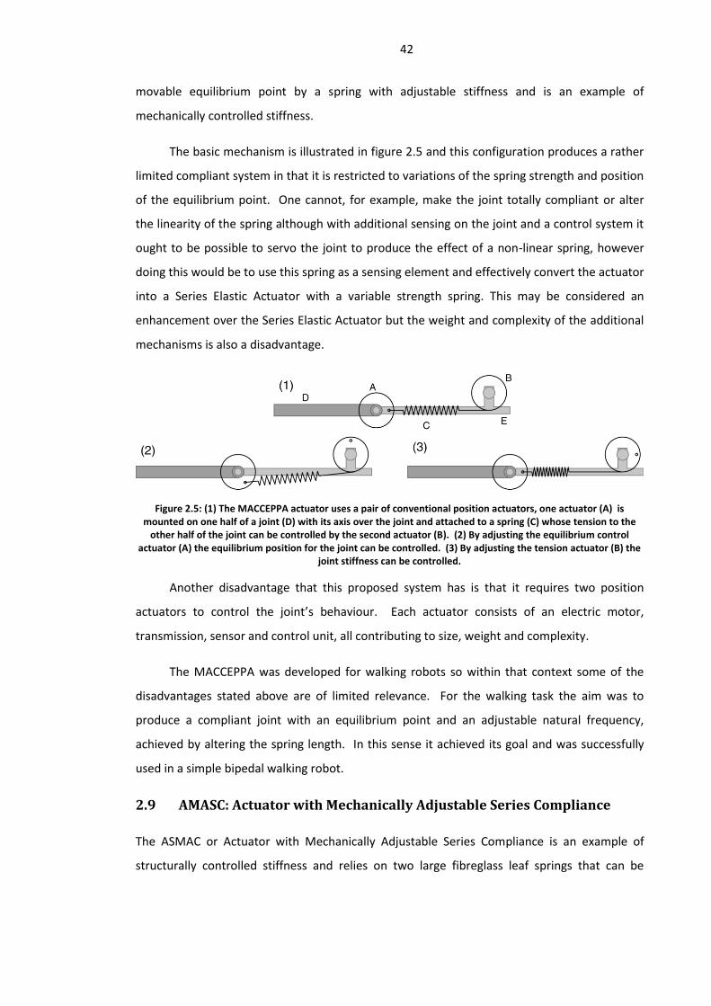
42

movable equilibrium point by a spring with adjustable stiffness and is an example of

mechanically controlled stiffness.

The basic mechanism is illustrated in figure 2.5 and this configuration produces a rather

limited compliant system in that it is restricted to variations of the spring strength and position

of the equilibrium point. One cannot, for example, make the joint totally compliant or alter

the linearity of the spring although with additional sensing on the joint and a control system it

ought to be possible to servo the joint to produce the effect of a non-linear spring, however

doing this would be to use this spring as a sensing element and effectively convert the actuator

into a Series Elastic Actuator with a variable strength spring. This may be considered an

enhancement over the Series Elastic Actuator but the weight and complexity of the additional

mechanisms is also a disadvantage.

Figure 2.5: (1) The MACCEPPA actuator uses a pair of conventional position actuators, one actuator (A) is mounted on one half of a joint (D) with its axis over the joint and attached to a spring (C) whose tension to the

other half of the joint can be controlled by the second actuator (B). (2) By adjusting the equilibrium control actuator (A) the equilibrium position for the joint can be controlled. (3) By adjusting the tension actuator (B) the

joint stiffness can be controlled.

Another disadvantage that this proposed system has is that it requires two position

actuators to control the joint’s behaviour. Each actuator consists of an electric motor,

transmission, sensor and control unit, all contributing to size, weight and complexity.

The MACCEPPA was developed for walking robots so within that context some of the

disadvantages stated above are of limited relevance. For the walking task the aim was to

produce a compliant joint with an equilibrium point and an adjustable natural frequency,

achieved by altering the spring length. In this sense it achieved its goal and was successfully

used in a simple bipedal walking robot.

2.9 AMASC: Actuator with Mechanically Adjustable Series Compliance

The ASMAC or Actuator with Mechanically Adjustable Series Compliance is an example of

structurally controlled stiffness and relies on two large fibreglass leaf springs that can be

43

adjusted via an actuator to alter the stiffness of a joint [74]. A second actuator allows the

equilibrium position of the joint to be controlled.

Figure 2.6: The ASMAC actuator (left) and its schematic representation (right).

The ASMAC is, like the MACCEPPA, designed for walking and running robots and

produces conditional compliance about a controllable equilibrium point. It is intended to

provide variable stiffness in the sense of creating an equilibrium point for the joint at an angle

which can be adjusted and with a spring force that can also be adjusted. In this sense the

degree of compliance is very limited but the adjustable passive springs do allow for an

energetically efficient system when applied to the right tasks. One major disadvantage of this

system is the complexity of the mechanical design, resulting in a large and presumably heavy

device.

2.10 VSA: Variable Stiffness Actuator

A third actuator that uses mechanically controlled stiffness is the Variable Stiffness Actuator

proposed by Tonietti et al. [75]. Like the previous two that have been discussed it employs a

pair of actuators to dually control the stiffness and equilibrium position of a sprung joint.

Figure 2.7 illustrates this design which employs a triangular arrangement of toothed pulley

wheels. One pulley connects to the mechanical output whilst the remaining two are powered

by electric motors. All three are coupled together by a pulley belt and between each pulley

wheel a certain amount of slack is maintained and tensioned by three sprung idle wheels.

Moving both motors synchronously allows the equilibrium position of the output to move,

whilst adjusting one motor at a time (or both in opposition) allows the tension of the springs to

be altered, affecting the stiffness of the joint.

44

Figure 2.7: The Variable Stiffness Actuator. The output lever connects to a pair of motors via a toothed pulley wheel and belt which is tensioned by three springs. Varying the relative positions of the two motors can tighten

or loosen the joint whilst moving the motor’s synchronously will move the lever’s equilibrium point.

This design has the same benefits as the previous two, namely that of energetic

efficiency, but also has the expense of requiring a pair of actuators to operate a single joint.

2.11 PAM: Pneumatic Artificial Muscles or McKibben actuators

All the previous actuators have been examples of electrically powered devices, although the

Series Elastic Actuator is not limited to electric drive. The PAM actuator by contrast is an air

powered device that has been used in some experimental robotics.

The design originally called the McKibben Artificial Muscle is based on the concept of a

conventional pneumatic piston where air pressure is used to force a plunger along a tube,

generating movement. The PAM variant dispenses with the rigid tube and plunger and

instead uses air pressure to inflate a rubber bag with a braided outer sheath. As the bag is

inflated the braids cause it to contract in length and as such it can be used as a single direction

actuator capable of pulling on a load. In this sense it is similar to a biological muscle which can

pull but not push.

This uni-directionality means that pairs of actuators are required to fully control a one

degree of freedom joint. When compared to electric devices the pneumatic air muscle is

relatively simple and light weight but, when the mechanisms required to deliver pressurised air

are factored in, these weight advantages begin to disappear.

45

Figure 2.8: A Pleated Pneumatic Artificial Muscle from Vrije Unversiteit Brussel, shown in three stages of contraction as the internal air pressure is increased.

When operating together as an antagonistic pair these actuators can function to alter

the stiffness and equilibrium point of a joint in the same fashion as the previously outlined

devices, however unlike these electrically driven and spring tensioned systems the PAM has a

non-linear response to its actuation position (length) and the force it generates. The PAM is

also naturally compliant because it relies on gas pressure to actuate and this gas is

compressible. A variant of the PAM called the PPAM or Pleated Pneumatic Artificial Muscle

has been developed [76] that reduces some friction and hysteresis problems associated with

the design. A large number of other variants have also been developed and a good overview

of the technology is provided by Daerden & Lefeber [77].

2.12 Discussion

The range of actuators presented above is by no means exhaustive but they represent some of

the mechanisms that have been designed for robotic applications over the past decade or so.

There are some other actuators that I have not mentioned, for example the use of shape

memory alloys and electro active polymers, which can be used as antagonistic actuators but

are still experimental in nature.

All of the actuators presented here possess a degree of natural compliance; however the

Series Elastic Actuator and direct drive systems do not have directly variable compliance in the

sense of being able to adjust the passive stiffness of a joint. The Series Elastic Actuator can

behave as a variable stiffness joint given the right control system, as can the direct drive

system.

46

Although the three passively adjustable compliant actuators described in sections 2.8-10

allow for control over passive joint stiffness and equilibrium position, this is restricted to

stiffness in the sense of the strength of a pair of springs that prescribe the equilibrium

position. If we want to introduce damping into the joint then we must either modify the

mechanism to include a variable damper, with added complexity and mass, or we can drive the

equilibrium position actuator to reproduce the effect of damping. The advantage of having

adjustable passive compliance where it requires no energy input to maintain a specific

compliance setting, only to adjust it, is offset by the fact that the compliance is highly limited.

The springs’ linearity is fixed regardless of their adjusted stiffness and the more general

structure of the joint, namely an equilibrium point with adjustable springs, is also fixed. One

cannot, for example, remove the springs from the joint entirely, or separate them in the

manner of an antagonistic joint with relaxed muscles. Although it is possible to reproduce

these effects by adding a control system to adjust the equilibrium point, this is in effect

reproducing the behaviour of the Series Elastic Actuator so although one could argue that the

resulting ‘Series Elastic Actuator with Adjustable Passive Compliance’ is the best of both worlds

it is also a more complex and heavier device, and only presents an advantage in circumstances

where this passive compliance can be heavily utilised.

With the PAM and PPAM actuators we have the same problem but with the added

complication introduced by the force and contraction non-linearity inherent in these designs.

The energetic efficiency of the passive adjustable compliance mechanisms can in part be

replicated by the direct drive system as well as the Series Elastic Actuator, although this

depends on the specific mechanical implementation. An electric motor can function as a

generator and produce electrical energy when the motor is moved, this is a technique often

found in electric vehicles where kinetic energy of the vehicles’ motion is reclaimed under

breaking, a technique typically called ‘regenerative breaking’. It can be possible to use this

property in a similar manner to a mechanical spring by absorbing kinetic energy from a joint in

motion. With a spring this energy will be returned immediately to the joint with high

efficiency but with the regenerative motor this energy will be stored in a battery or capacitor

where it can be re-used by any of the electrical systems. Although the electronic version is less

efficient at re-cycling energy than a mechanical spring it does offer a more flexible method

because the reclaimed energy can be stored for long periods and re-used anywhere in the

system.

47

2.12.1 Selecting an actuator for this research

Within the selection of actuators above we can find designs that may be a best fit for various

different tasks however the goals of this research are to develop a general purpose controlled

compliance actuator and as such the most versatile design is the most appropriate.

The Series Elastic Actuator presents the most useful design in this respect because it is

relatively simple but functions as a good source of force that is independent of position. The

direct drive motor also presents a good solution as a source of force but it generates low

torques whilst being relatively heavy and power hungry which is an issue, particularly if used

with mobile (battery powered) robots.

Because of its general functionality I have based most of my work on the Series Elastic

Actuator as a design worth developing and applying to various robotic tasks. In the next

chapter I will outline some of the early attempts to refine and simplify the Series Elastic

Actuator in order to produce a low cost revolute system based on this design. This will help to

illustrate how experiments with this design led to the conception of the ideas at the heart of

this thesis and which formed the basis for the rest of my research, namely the design of an

electro-mechanical emulator for mechanical joints.

48

Chapter 3

Early attempts at reproducing the Series Elastic Actuator

The previous chapter explored how controlled compliance can be of value in creating robots

that perform well at certain tasks. It also examined some designs for actuators that could be

used in these types of robot. I will now move on to document my own foray into this field.

This chapter will discuss some early experimental work I started but later abandoned as some

discoveries during design and testing of these experiments led me to change the focus of my

research, which in turn led to the work presented in this thesis. This chapter helps to provide a

context for the genesis of this thesis and introduces a few key concepts that underpin the rest

of the work.

My early attempts to develop controlled compliance actuators concerned their

application in powered passive dynamic walking robots where we required an actuator that

could apply torque to a joint at certain points during walking whilst remaining fully compliant

at other points. In parallel to this was an interest in building manipulators with inherent

compliance for safe human robot interaction. Both these avenues of interest required the use

of actuators that could control the force they generate and the Series Elastic Actuator was

selected as a basis for my own work because of its relative simplicity and good performance.

The Series Elastic Actuator designs developed at MIT and later commercialised through

Yobotics present a linear actuation system and are designed to be operated in a muscle like

fashion to control a rotary joint, although unlike a muscle it is capable of both pushing and

pulling. For my own work I wanted to integrate the actuator into a single degree of freedom

joint along with sensors for the joint’s angle. This also required the production of a revolute

rather than linear elastic force sensor.

The basic design for the joint consisted of a motor and gearbox driving an output lever

via an instrumented elastic coupling. This coupling connected the motor to the lever via a set

of silicone rubber bushes such that torque transmitted through the bushes would cause them

to compress. This would then be reflected in the instrumentation which measured the angle

difference between the two halves of the coupling. This setup therefore provided a crude

49

method of measuring the force at the joint and was then used by a simple control circuit to

drive the motor. The control circuit consisted of a microcontroller which would read the force

sensor and an implementation of a proportional derivative or PD algorithm that would drive

the motor to maintain a specified deflection in the coupling. A more detailed description of

this elastic force sensor and its control system are covered in the next chapter.

In order to validate, at least in general terms, the behaviour of this actuator I attempted

to construct a two jointed planar arm that could be used to replicate a series of experiments

performed with the robot COG.

3.1 Crank turning experiment

The experiments performed with COG, which used Series Elastic Actuators in its arm joints,

was used to test ideas regarding the benefits of compliance in generating robust adaptive

motion using minimal control [18-20]. The robot was set up with an arm connected to a crank

and the intention was to produce motion in the arms using simple neural oscillators driving

each of the Series Elastic Actuators. None of the actuators were connected electronically; the

only means by which they could communicate was physically via the environment and the

robot’s mechanical structure.

Figure 3.1: COG, a humanoid torso developed at MIT.

Although not directly incorporating angle sensing, the Series Elastic Actuators used in

COGs arms were employed for every joint, and each of these joints incorporated an angle

sensor. A simple compliant control system was devised whereby each degree of freedom was

controlled by specifying an angular set-point, which in turn was used to generate an error

50

signal. This error signal and the error velocity were both then multiplied by respective gain

values (one for the error and one for the error velocity) before being summed and used to set

the force output of the Series Elastic Actuator.

The resulting system, in terms of an individual actuator and its angle sensor, then

behaved like a controllable linear spring damper where the joint was held at an equilibrium

point (the set-point) by a pair of spring dampers. The strength of these spring dampers could

be determined dynamically by altering the error and error velocity gain values. This system

was, within certain limits, functionally equivalent to the structurally or mechanically controlled

compliant mechanisms described in the previous chapters but relied on software to generate

the effect of springs and the resulting equilibrium point. It also had the advantage of including

damping as a separate controlled parameter.

The experiment showed that with simple neural oscillators controlling the angle set-

point for each degree of freedom the robot arm would naturally ‘find’ a cyclic motion that

would drive the crank perpetually around. They found that this system was relatively immune

to changes in various parameters and required no communication between actuators, save

that which was gained through physical coupling. This result was in stark contrast to how the

problem of generating the right motion to turn the crank would be solved by traditional angle

and velocity controlled actuators. The traditional solution would require some analysis of the

crank and the kinematic constraints it imposed on the movement of the arm before a set of

motion parameters could be planned and executed, resulting in the arm reproducing the

correct motion and driving the crank. In short the simple compliance of the joints and the way

it allowed the kinematic constraints to modulate the neural oscillators removed the

requirement for more complex sensing, analysis and inverse kinematics.

The apparent success of this approach to joint control provided me with a starting point

for my own investigation; in particular it seemed a good way to test my own compliant

actuator.

3.2 Experimental setup

Rather than attempting to reproduce a fully articulated arm I chose to reduce it to the simplest

system that could perform the crank turning task whilst requiring a degree of co-ordination

between the actuators to achieve this. The arm, a section of which is shown in figure 3.2,

consisted of a two jointed mechanism with one end fixed to a frame, and the other end driving

a lever via the elastic actuator. A second elastic actuator was attached to the end of the lever

51

to form an elbow to another lever. The end of this lever then attached to a crank handle

which was instrumented so the number, rate and direction of turns could be recorded.

Figure 3.2: A single jointed arm with a crude Series Elastic Actuator built into the joint. To complete the mechanism a second actuator would be attached to the end of the arm creating an elbow.

Rather than replicate exactly the neural control system used by Williamson et al. I had

intended to start with a simple software oscillator generating a saw tooth signal that would be

used to specify the force outputs of the elastic actuators. I had hypothesised that by adding a

modulating variable to the oscillator and linking it to the angle I might be able to produce a

system that would settle into a cyclic motion and perpetually turned the crank without having

to instantiate the more computationally complex neural net controller used by Williamson.

3.3 An early experiment and a change of goal

The process of constructing the arm and testing led to an observation that even the simplest of

oscillator would generate cyclic (Crank turning) motion without any force control. When

testing the motor controllers and ensuring that the mechanism was capable of turning the

crank I connected the motor controllers to a joystick so the X and Y axis provided a source for

setting each motor’s drive voltage. By moving the joystick left and right I could move one

motor and by moving it up and down I could control the other.

I discovered that simply by moving the joystick in a circular fashion the arm would turn

the crank and by adjusting the speed of my movement the arm would also adjust its rate. This

was unsurprising in the sense that my motion of the joystick was co-ordinating both motors

but it did make it apparent how easy it was to produce the correct motion and this appeared in

part to be due to the compliance inherent in each joint. Although the force control system had

not been implemented the rubber bushings that were used to couple the motor to the load

provided a degree of natural compliance that helped with the task.

52

These observations led me to consider that this experiment, in particular my over

simplification of Williamsons setup might be of little value.

3.4 Converting the PD force controller to an antagonistic controller for

walking

Rather than abandon the experiment entirely I decided to re-focus my work by looking at how

a Series Elastic Actuator could be used to reproduce the effect of a pair of antagonistic,

muscle-like actuators, acting to control the arm. This was of particular relevance to attempts

at creating powered passive dynamic walking systems.

In contrast to the cyclic arm tasks the walking task required that the joint became

completely passive at certain times to allow the leg of a bipedal robot to swing forwards in the

manner of a pendulum. The sprung and damped equilibrium point system used in the arm

experiments by Williamson et al only allowed the forces in the joint to be set to zero by setting

the proportional and derivative gains of the controller to zero, however when re-instating

compliant control one would also re-instate the equilibrium point which, without extra

software might end up in a different place to the leg joint. It seemed that a better method was

to instantiate a kind of virtual antagonistic pair of spring dampers that could be shifted about

the leg joint’s angle. This would allow you to create a zone of compliance, a range of angles

where no force was applied by the actuator, bounded by a set of adjustable spring dampers.

These spring dampers could then be moved around to alter the size of this compliant zone

and, if brought together, replace it with an equilibrium point.

Figure 3.3 illustrates this concept with the graph representing the angle of the joint and

the force output of the elastic actuator. Two virtual springs, X and Y were created by

specifying a starting angle and a spring constant. For each spring a force value could be

calculated by measuring the distance that the joint had gone beyond the spring start position

and multiplying it by the spring constant. Moving the start positions around had the effect of

moving the springs around whilst adjusting the spring constants would alter their stiffness. An

identical set of constants could then be used to specify damping for each spring. With this

setup not only could you move each spring around independently and create zones of zero

impedance, you could also create asymmetrical compliant joints where the spring damper on

one side of the equilibrium point was different than the other.

53

Figure 3.3: A graph representing force to angle relationships. The desired or target force on the vertical axis is plotted against the measured angle along the horizontal axis. A starting angle (A or B) represents the start of a spring (X and Y) whose strength is determined by a spring constant variable, this is represented by the slope of

the line on the graph. Altering the spring constant variable will alter the slope and altering the starting angle will move the spring around.

3.5 Creating force tables from graphs

The graph in figure 3.3 marks the genesis of the rest of the work in this thesis. It is a visual

depiction of a complex mechanical spring system in a rotating joint but it is defined by a series

of equations that describe the mapping of angle to force. Whilst this is nice and simple when

generating the linear springs shown in the graph it becomes more complex if we want to add

extra spring systems to the joint or if we want to make these springs non-linear. With

increasingly complex springs we might find that the resources needed to compute the required

functions could easily outstrip the resources available on an embedded controller that one

might use in this type of actuator, and that of course assumes that a suitable non-linear

function can be devised.

An alternative to this problem of a computed spring system would be to approximate

the spring function using a look up table. Instead of computing the force output for the elastic

actuator the control system could simply look up a pre-defined value in memory and apply it.

It would then be possible to specify any force value for any quantised angle, allowing you to

specify arbitrary spring functions across all angles and with a similar system for damping we

could also specify damping across all angles. With this system the actuator would be pre-

configured with user data in the two look up tables and its control loop would consist of simply

reading its angle and angle velocity, looking up the appropriate force value for the current

angle then subtracting out the current velocity multiplied by the damping value for the current

angle. The result of this calculation would then be passed to the elastic actuator control

system as a force for it to generate.

54

The number of angles that the actuator could be at, and consequently the number of

values required to build the look up table, could be impossibly high were it not for the fact that

converting a finite angle to a digital value requires that we reduce the actual angle to a

discrete, quantised value. In other words we can only read the actuator’s angle with a limited

resolution. In the case of the class of microcontroller that we would expect to control this type

of actuator we might get 10 or 12 bits of resolution resulting in angle values that can be

anywhere between 0 and 1023 or 4095. If we were to assume that the resolution of the force

generating control system (the PD controller responsible for the elastic actuator) was similar

then, with ten bit resolution for our angle sensor, our look up table becomes 1024x2 bytes in

size or 2048 bytes (I assumed that each force value would use no more than two bytes of

memory). If we add in a similar look up table for damping then we end up using 4096 bytes to

describe what could be a totally arbitrary spring damping function across all measurable angles

for the actuator. The cost of this with respect to memory is minimal and easily accommodated

by most microcontrollers.

Of course the memory demands will increase as we increase the resolution of digital

conversion applied to the angle sensor but the resolution limits placed on us by the hardware

also apply to the computed spring systems previously described. In some instances the ten bit

resolution described above is more than required and a smaller look up table can be used in

conjunction with an interpolation algorithm to make up values for intermediate angles.

Figure 3.4 illustrates a spring and a damping table and shows how arbitrary values can

be used to define complex spring damping systems for the actuator to reproduce. The force

and damping values are used in conjunction with the angle velocity to calculate a final force

value for a given angle as follows:

Tf = Fa-(V*Da)

Where Fa is the value in the force table for the current angle, V is the angle velocity and

Da is the value in the damping table for the current angle. The value of Tf is the target force

used to command the Series Elastic Actuator.

The method of computing a damping force in this system produces an effect

approximate to viscous damping where the magnitude of the damping force scales with

velocity. This type of damping is the same as that used in the experiments with COG and is

inherited from more traditional motion control approaches where the derivative term of a PD

controller also produces a damping force that scales with velocity, and is analogous to viscous

55

damping. Other types of damping also exist in mechanical systems and can better capture

some effects found in natural systems, for example in sliding friction where the friction of a

static object on a surface is higher than when it is in motion. These issues are discussed in

chapter 7.

Figure 3.4: Using look up tables to define functions can allow arbitrary spring and damping systems to be defined. The force table (top) illustrates a variety of spring systems defined with force values across angles and the damping table (bottom) illustrates how similarly versatile damping zones can be defined across all angles,

including negative damping values which would amplify rather than resist motion. Areas of equilibrium exist where the values are at zero force, and these can either be stable or unstable.

3.5.1 Problems with using tables for dynamic functions

The use of look up tables might seem attractive in terms of being able to create arbitrarily

varied springs and dampers across all angles; however it requires a relatively large amount of

data to describe a complete system compared to the computed version. If we take a simple

example with an identical pair of linear springs that create an equilibrium point then describing

this with the look up table will require 2048 bytes (assuming we use the same resolutions as

described above) but describing it in terms of an equilibrium point and a spring constant may

only require four bytes, two for the equilibrium point and two for the spring constant. If we

also want damping for the springs then we need another two bytes as opposed to another

2048 for the look up table.

This difference in data quantity becomes a serious problem when we want to modify the

parameters of the springs, dampers and equilibrium points whilst the actuator is working.

Assuming we are communicating with the actuator over a serial data link then in order to do

56

this with the computed system we need only transfer between four and six bytes, but the look

up tables require up to 4096 bytes. The advantage of the arbitrary spring and damping

functions is countered by the increase on communication overheads and the problem of how

the system should behave whilst new data is being uploaded.

3.6 Biasing and scaling angles to modify tables

If we want to reproduce some of the same functionality of the computed linear spring system

with our look up table, namely the adjustable spring constants and movable equilibrium point,

without incurring the communications overhead then we need to introduce some method of

modifying the look up table, or at the very least its results.

If we want to move any equilibrium points about then we can actually achieve this

relatively easily by biasing the angle that the control system is reading. By sending the

controller a single variable and adding this to the angle as read by the controller it will index a

different force and damping value than normal.

Figure 3.5: A force table can be modified by applying a bias and scale to the angle used to index its values. The values in the normal (unmodified) table are shown along with the apparent values after the angle is scaled by 0.5 or biased by 60 degrees. An equivalent computed system would calculate a spring force by using a set-point (A) which can be moved to different angles (for example B), and a spring constant multiplied by the distance of the

angle from the set-point. Doubling the spring constant (C) will produce a steeper slope (D) which is equivalent to scaling the measured angle by 0.5.

We can apply a similar technique to alter the spring constants defined in the profile by

scaling the apparent angle of the actuator. If we want to make the springs stronger or weaker

then we simply multiply the measured angle (relative to the equilibrium point) by a control

variable and this will have the effect of altering where in the look up tables the value is

obtained with respect to the actual angle.

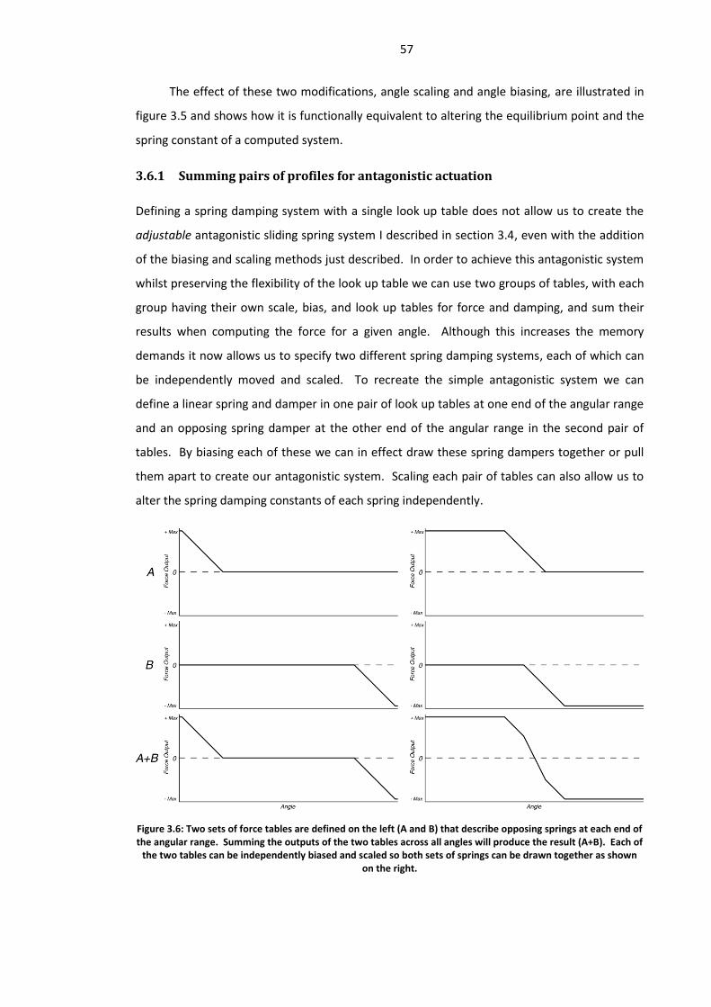
57

The effect of these two modifications, angle scaling and angle biasing, are illustrated in

figure 3.5 and shows how it is functionally equivalent to altering the equilibrium point and the

spring constant of a computed system.

3.6.1 Summing pairs of profiles for antagonistic actuation

Defining a spring damping system with a single look up table does not allow us to create the

adjustable antagonistic sliding spring system I described in section 3.4, even with the addition

of the biasing and scaling methods just described. In order to achieve this antagonistic system

whilst preserving the flexibility of the look up table we can use two groups of tables, with each

group having their own scale, bias, and look up tables for force and damping, and sum their

results when computing the force for a given angle. Although this increases the memory

demands it now allows us to specify two different spring damping systems, each of which can

be independently moved and scaled. To recreate the simple antagonistic system we can

define a linear spring and damper in one pair of look up tables at one end of the angular range

and an opposing spring damper at the other end of the angular range in the second pair of

tables. By biasing each of these we can in effect draw these spring dampers together or pull

them apart to create our antagonistic system. Scaling each pair of tables can also allow us to

alter the spring damping constants of each spring independently.

Figure 3.6: Two sets of force tables are defined on the left (A and B) that describe opposing springs at each end of the angular range. Summing the outputs of the two tables across all angles will produce the result (A+B). Each of

the two tables can be independently biased and scaled so both sets of springs can be drawn together as shown on the right.

58

Figure 3.6 illustrates the results of summing two force profiles to produce an

antagonistic system with the springs pulled apart and then drawn together.

3.6.2 Creating hysteresis with angle thresholds

The examples so far have illustrated how we can use look up tables instead of computed

functions to specify arbitrary spring damping systems in an actuator. The inclusion of a second

set of spring damping tables and the method of biasing them with respect to the angle allows

us to create independently adjustable antagonistic springs. What this approach can’t do is

allow us to create hysteresis in the system. What if we want the entire spring damping system

to be replaced with a different one when the actuator passes a certain angle in order to create

behaviours like latching?

If two sets of spring damping tables are available in the actuator, as is required for the

antagonistic system, we can also employ them to create this hysteresis. Instead of using them

concurrently and summing their outputs we use them individually and specify an angle for

each that, when passed, will cause the control system to swap over to the alternate set of

tables.

Figure 3.7: Using pairs of tables to create hysteresis. Force Table A is given an angular threshold X and force table B is given an angular threshold Y. When using table A, and the system’s angle goes below X, it will swap over to table B. Going above threshold Y will cause it to swap back to table A. The arrows indicate how and where the

system alternates between the two tables with respect to its current angle. With the two force tables as defined above the behaviour will reproduce that of a symmetrical sprung latch.

By allowing one set of angle thresholds to be defined for each set of spring dampers,

alongside the biasing and scaling that each already has, we can now create more complex

classes of spring damper that include hysteresis. Figure 3.7 illustrates how a pair of spring

tables can be given thresholds for their angles that cause the actuator to jump over and start

using the alternative set of tables. In this example the result will be a mechanical latch that

remains in one position until perturbed beyond its threshold, at which point it will prefer the

alternate position. If memory resources permit it then we can also include even more groups

59

of look up tables and their associated parameters allowing us to configure the actuator to

reproduce even more complex mechanical behaviours.

3.7 Actuators as general purpose mechanical emulators

Using multiple look up tables grouped with a set of modifying variables and conditional checks

can potentially be used to allow a force controlled actuator to emulate various mechanical

spring damping systems. The way these spring damping systems can be easily represented

visually also means that they can potentially be specified intuitively by literally drawing the

spring function that you want. This insight into the versatility and ease of use that this

approach offered had the effect of ending my tentative excursion into creating compliant arms

and legs for robots and instead shifted the focus of my work on to refining and understanding

how the approach outlined above could be used to turn force controlled actuators into general

purpose emulators of mechanical joints.

By putting a high level of functionality into a modular device and providing an easy

method of configuring the various parameters, the process of experimenting with dynamic

robotic systems could become far easier than trying to construct entirely bespoke systems.

With the correct physical design an actuator could be easily employed to create a variety of

joints with a minimal amount of engineering, and by embedding a control system

incorporating the table based behaviours into each device it would be possible to rapidly and

easily reconfigure the mechanical properties of the joints. Even if a joint only required some

fixed spring or damper one could, in an experimental situation, employ one of these devices to

emulate the fixed springs allowing their values to be altered in software rather than by re-

engineering the hardware.

3.8 Summary

Previous chapters have tried to provide both a justification for the use of controlled

compliance in robotic systems and a historical context for their development, followed by

some examples of devices that have been developed for autonomous and biologically inspired

robots. This chapter has looked specifically at how my own early experiments with creating

compliant robots led to the actuator and control system that has been the focus of my

research ever since. This illustrates how my early work with specific robotic systems, namely a

simple arm and a powered passive dynamic walking system, led me into these attempts to

create a more generalised actuator that I could use to create these robots.

60

I have used the term damping in this chapter to refer to a force that opposes motion

and which is proportional to velocity, this type of damping is a standard component of motion

control systems, in particular PID and PD controllers where the derivative term (D) is typically

referred to as damping. In mechanical terms this type of damping is a model of viscous

damping but it is not the only type of damping force that exists.

As I previously stated in my introduction, the subject of this thesis is in many respects a

means to an end. I want to make robots with interesting, dynamic and adaptive behaviour and

it is a lot easier to do this when you have access to the appropriate component parts. The

remainder of this thesis will expand on the control concept that I have outlined in this chapter.

I will begin by providing some more detail of the mechanical and electronic designs that I have

experimented with in an attempt to create a relatively compact modular actuator with an

integrated controller that could reproduce all of the functionality I have described here.

Once I have covered the mechanical and electronic designs used in my research I will

move on to describe the control system itself. This represents a more refined version of the

system of look up tables and thresholds described in this chapter and following that I will

provide some examples of how this control system can be used to create a variety of

mechanical systems within a single actuator and then with multiple interacting actuators.

Chapter 6 will also provide results from real devices using these configurations and also help to

highlight some issues and limitations of the system. These limitations, and others such as the

types of damping that the system can produce, will then be discussed in more detail in chapter

7 where I will also propose some solutions to problems, and enhancements to the control

system.

61

Chapter 4

The Programmable Spring: Electronic and mechanical design

overview

The previous chapter has introduced a method of creating tables of data to act as a transfer

function between a force controlled actuator’s angle and angular velocity, and its force output.

This can potentially allow you to sculpt arbitrary spring damping systems for the actuator to

emulate. By adding extra tables grouped together with controllable thresholds for angle, and

a method of switching between the different tables we can emulate spring damping systems

with hysteresis. By summing different tables and biasing the apparent angle we can emulate

the action of antagonistic pairs of adjustable springs and dampers. These concepts form the

core of a potentially novel control system that allows a force controlled actuator to emulate a

variety of mechanical systems. In the chapter following this I will take a detailed look at how

this concept has been expanded into a more comprehensive control system, but first I will take

a look at some of the hardware that has been developed on which this control system will run.

I will start by examining the issue of elastic force sensors which are required if a Series

Elastic Actuator is to be used as the basis for the force controlled actuator. Following this I will

detail the electronics used to control the actuator and then give some consideration to the

actuator’s morphology. Describing these electronic designs is important as they detail some

features that are exploited by the control system and as such the proceeding chapter will

reference them at various points.

4.1 Designing an elastic force transducer

Designing and making a bespoke elastic force transducer might at first seem to be a trivial task;

after all it essentially consists of a spring and a sensor to measure the degree of compression

or deflection of the spring. In reality the task is a little more complex and resulted in a number

of different designs, some better than others. Some of the constraints that made this design

process more difficult were those imposed by the actuator design I had in mind. I wanted to

produce a compact unit with a revolute output; this was in contrast to the normal

embodiment of a Series Elastic Actuator which had a linear output. Producing a linear force

62

transducer is a relatively simple design task as it consists of a pair of compression springs and a

sliding potentiometer to measure displacement. An alternative design that still employed

compression springs had been proposed [68] but this was not suitable for my purposes

because of its awkward shape. The principle of the linear system and the rotary derivative are

shown in figure 4.1.

Figure 4.1: Linear and rotary elastic force transducers. Left: A linear elastic sensor using a pair of die springs to transfer the force between a linear actuator and an output and employing a linear potentiometer to sense the

spring deflection. When there is zero force difference the sensor remains in the centre (A) and generating a force difference will change the spring compression (B). Right: A revolute elastic coupling using a pulley, cable and

piston arrangement to operate a pair of die springs. A potentiometer mounted on the axis of rotation would be used to measure the spring deflection caused by a force difference between the input and output. Parts C and D

show how force differences affect spring compression.

One key advantage cited for using compression springs in both of these designs was the

fact that they could be purchased ‘off the shelf’ as stock parts rather than requiring the

production of potentially expensive custom torsion springs. My own design limitations

required that any torque transducer would be capable of driving a rotating shaft and fitting

into a compact housing, so it was difficult to find any off the shelf parts from which a suitable

design could be created.

A cost consideration I made during the design process was that of manufacturability.

Because one of my goals was to create a functional building block for general purpose robotics

research any design for the torque transducer that was too costly or difficult to manufacture

would undermine that goal.

In terms of the mechanical performance of the sensor it had to perform several

functions. Because it was designed to drive a rotating shaft in both directions it needed to be

capable of sensing force in both directions. As force was applied to the device it would need to

transfer it across the elastic element to its other half and, in the process, cause the elastic

element to deform and the two halves of the transducer to alter their relative angles. This

deformation had to be proportional to the forces being transferred through the sensor and

63

have a maximum deformation that was greater than the maximum torque that the motor

could generate. The force sensor also had to return to the same position each time the same

force differential was applied so that it did not require constant re-calibration.

In the following sections I will describe a number of candidate designs for simple elastic

force sensors. Three of the designs were constructed and evaluated with a test rig to establish

how they responded to a varying torque.

I constructed a very simple manual force measurement system using a spring based

hanging weight gauge as shown in figure 4.2. This spring weight gauge pulled on a cable that

wrapped around a pulley which could be attached to one half of the rotary sensor; the other

half of the sensor was fixed to a bench to prevent it from moving. The pulley was six

centimetres in diameter so by pulling on the weight gauge it was possible to control the

number of Newton meters of torque applied to the sensor. The sensor was equipped with a

potentiometer connected as a potential divider to a power supply and a multi-meter, allowing

the sensor’s displacement to be read electronically. The response of the potentiometer to

angular change is linear with a tolerance of approximately one percent and it was powered

from a symmetrical +/- 6 volt power supply so that the sensor, when at rest, would produce a

reading of approximately zero volts. These values were then normalised to a range of +/- 1.0

across the full voltage range.

These were not intended to be precise tests of the sensors but were intended to map

out the force to displacement characteristics of each sensor. A series of readings from the

multi-meter were taken as the pull on the gauge was slowly increased. All the results shown in

the following sections show a plot of the voltage output of the potentiometer against the force

displayed by the spring gauge as the tension is increased. The tests were repeated for both

directions of rotation with positive forces denoting clockwise rotation of the pulley and

negative denoting counter clockwise.

Figure 4.2: A spring weight gauge and pulley wheel attached to one of the rotary force sensors.

64

4.1.1 Rubber force transducer

The first attempt to create a revolute elastic force transducer appeared to provide an ideal

solution and involved the use of rubber as the elastic element. Figure 4.3 illustrates the design

alongside a photograph of a test device. The basic design involved a round barrel shaped

enclosure with a pair of internal tabs. At one end of the barrel a hole accommodated a

bearing and the other end accommodated another bearing seated in a removable cap This cap

could be constructed from a spur gear and acted to connect the motor and transmission to the

sensor.

Figure 4.3: A rubber based force sensor consisting of an outer barrel and inner shaft coupled together with rubber bushes via tabs on each part of the device. Normally the rubber keeps the two parts in a central position (A) but

a force difference will cause one pair of rubber bushes to compress (B). The outer part would be driven via a spur or bevel gear and transfer the torque to the output shaft via the rubber. A potentiometer can be used to

measure the displacement.

The output shaft fitted through the centre of the barrel and was kept in place by the

bearings. This shaft had a pair of tabs attached to it which were situated inside the barrel so

that the barrel could rotate by approximately sixty degrees relative to the shaft before the tabs

inside the barrel and the tabs on the shaft came into contact and prevented any more

movement in that direction.

A series of rubber bushes were fashioned that would fit snugly on either side of the

shaft’s tabs so that it was held in a position half way between the barrel tabs. When fully

assembled any force differential applied to the device would be transferred from one half to

the other by these rubber bushes, which in turn would deform at a rate proportional to the

force differential. This deformation could be measured by a hollow centre potentiometer

attached to the barrel of the sensor with the shaft poking through the centre of the

potentiometer so that relative angular differences between the barrel and shaft could be

measured.

65

One apparent issue with the use of rubber as the elastic element was the fact that the

way it deformed in response to applied force was non-linear. This meant that the reading

from the potentiometer would not be linearly proportional to the force difference. This may

not be a problem in that one could linearise the signal using software on a microcontroller, but

the exact nature of the non-linearity could affect how the final devices behaves mechanically

which in turn may require a more complex control algorithm.

The sensor was tested using the apparatus and method described above. The results

are shown in figure 4.4 and illustrate an interesting S shaped or sigmoidal response to force.

At low forces the amount of movement in the sensor is high and as the force increases the

angular displacement relative to a unit of applied force decreases.

Figure 4.4: The output voltage of a rubber force transducer as it is subjected to varying forces.

The result of using a sensor like this would be to produce a force generator that had high

sensitivity to low forces with an increasing insensitivity to variations in high forces. It might be

argued that this is actually an advantage for some tasks, for example a manipulator might be

required to exert large forces at some times but also to perform delicate tasks at others. An

analysis of the way spring design affects the performance of Series Elastic Actuators can be

found in the PhD thesis of David William Robinson at MIT, and he notes in his conclusion the

following with respect to non-linear springs [69]:

“Non-linear stiffening springs - Biological springs (tendons) are stiffening. One

theory behind this is that at low forces or during contact tasks the low stiffness helps

maintain stability. At much higher forces, low stiffness is unnecessary and may be even

undesirable.

Some initial theoretical and experimental work has been done previously in

applying non-linear stiffening springs to the actuators in fixed base robots [citation

66

omitted]. In this thesis, I show that there is a fundamental trade of between large force

bandwidth and impedance when choosing a spring stiffness. Low impedance requires a

soft spring whereas a soft spring reduces the large force bandwidth. Using a non-linear

stiffening spring may be a bridge between these requirements.

Stable control of series elastic actuators with non-linear springs may be as

simple as using a scheduling control gain that is a function of spring deflection. As the

spring stiffness increases, the control gain decreases proportionally. This keeps the loop

gain of the system constant and within stability margins.”

His analysis suggests that a non-linear spring may be of benefit to the general control of

the Series Elastic Actuator however he also notes the following about the properties of rubber

in particular:

“Hysteresis and materials - Most physical springs have some hysteresis. The die

compression springs used in this thesis have very little hysteresis and were assumed to

be linear in the control. It is suspected that with increased spring hysteresis, the

actuator becomes more difficult to control. For example rubber springs are often used

for vibration isolation because of inherent hysteresis and damping properties. Air

springs are often used for high force applications. However, they too have

thermodynamic hysteresis properties. Quantifying the effects of hysteresis would be an

important step to using new materials and springs in the actuators.”

The issue of hysteresis with respect to the stability of the elastic actuator is an important

one and hysteresis is a particular problem with rubber, especially in relation to a property

known as compression set. When compressed for long periods of time rubber will start to

deform permanently, this is usually known as compression set and is not a property usually

found in metal springs when they are used within their elastic limits. Compression set in a

sensor of the type outlined here can be a serious problem with respect to the calibration and

response of the sensor over time. If a sensor in a robotic joint were to be subjected to a

prolonged displacement, for example a leg joint supporting a body whilst the robot is inactive,

the sensor would begin to lose its calibration. One serious effect of this would be that the zero

force angle of the sensor would shift – this is the relative angle of the two halves of the sensor

at which there is no displacement of the elastic elements. If one elastic element becomes

deformed then this position will shift and if both become deformed there may even be a gap

between the two elastic elements that introduces backlash in the sensor.

67

Despite the potential offered by rubber as the elastic element in a force sensor, not to

mention the ease with which such a sensor could be manufactured, the problems with

hysteresis are serious and no obvious solution presents itself apart from the wholly impractical

approach of re-calibrating the sensor every time it is used. For these reasons I eventually

abandoned the idea of using rubber and sought a better solution.

4.1.2 Tuning fork

The second design I developed involved a tuning fork arrangement where a pair of leaf springs

kept a cam, attached to a central shaft, in place. The mechanism and a photograph is shown in

figure 4.5.

Figure 4.5: A force transducer based on a pair of leaf springs in a ‘tuning fork’ arrangement. The output of the sensor remains in the central position when at rest (A) and will deflect one of the two leaf springs when a force is

applied (B).

When a differential force is applied between the sensor body and shaft the cam will

push against one set of leaf springs causing them to deflect. The principal reason for the

design of this sensor was that spring steel could be used to construct the leaf springs and, at

the scale and force ranges I was working to, these springs could be easily created in our lab

using a set of shears. The body of the sensor was constructed from polyurethane poured into

a mould and the central cam consisted of a small bearing mounted on a tab that was fixed

onto the shaft. The bearing helped prevent any sliding friction as the cam bent the leaf springs

and slid along their length.

Some consideration had to be given to the design of the sensor body, particularly where

the leaf springs were fitted. They were clamped in place with a metal tab inside the sensor

body and a curved wall prevented them bending too much at the clamping point, this was

important in allowing a strong spring to be used in a small package without causing a

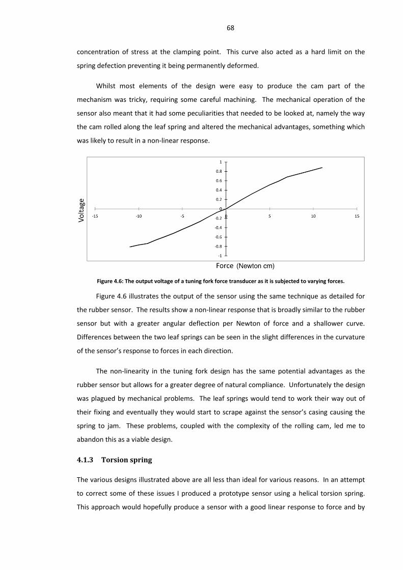
68

concentration of stress at the clamping point. This curve also acted as a hard limit on the

spring defection preventing it being permanently deformed.

Whilst most elements of the design were easy to produce the cam part of the

mechanism was tricky, requiring some careful machining. The mechanical operation of the

sensor also meant that it had some peculiarities that needed to be looked at, namely the way

the cam rolled along the leaf spring and altered the mechanical advantages, something which

was likely to result in a non-linear response.

Figure 4.6: The output voltage of a tuning fork force transducer as it is subjected to varying forces.

Figure 4.6 illustrates the output of the sensor using the same technique as detailed for

the rubber sensor. The results show a non-linear response that is broadly similar to the rubber

sensor but with a greater angular deflection per Newton of force and a shallower curve.

Differences between the two leaf springs can be seen in the slight differences in the curvature

of the sensor’s response to forces in each direction.

The non-linearity in the tuning fork design has the same potential advantages as the

rubber sensor but allows for a greater degree of natural compliance. Unfortunately the design

was plagued by mechanical problems. The leaf springs would tend to work their way out of

their fixing and eventually they would start to scrape against the sensor’s casing causing the

spring to jam. These problems, coupled with the complexity of the rolling cam, led me to

abandon this as a viable design.

4.1.3 Torsion spring

The various designs illustrated above are all less than ideal for various reasons. In an attempt

to correct some of these issues I produced a prototype sensor using a helical torsion spring.

This approach would hopefully produce a sensor with a good linear response to force and by

69

using a metal spring and controlling the string strength with respect to the desired working

angle it would never be pushed beyond its working range.

The main problem I faced with producing a design like this was that the required spring

was not available as a stock item from spring manufacturers. The design required a torsion

spring with a non-contacting coil arrangement where neighbouring coils did not make contact

with each other. This arrangement removed any friction caused by coils sliding against each

other and is a source of hysteresis. The springs also needed to be short, having at most a

couple of turns to provide a high spring constant over a limited working angle.

Unlike the rubber or the tuning fork sensors the torsion spring sensor requires only a

single spring if it behaves the same when being wound or unwound; this is not necessarily the

case and spring manufacturers recommend that torsion springs are loaded so that they wind

up (reduce their diameter) rather than are unwound, but for the sake of simplicity I have used

a single spring. It is possible to design a similar device to the one I will describe but using a pair

of pre-loaded torsion springs working in opposition to each other in order to produce a

mechanically correct and symmetrical design.

Figure 4.7: A force transducer using a torsion spring to couple a gear to an output shaft. The device is shown in cross section on the left and a photograph of the prototype fitted to an actuator on the right.

In order to avoid the cost of getting a torsion spring custom made I managed to find a

strong compression spring and adapt it to fit a mechanism that would wind or unwind the

spring in response to a force differential between a shaft and a gear. This use of a

compression spring had the automatic advantage of producing a torsion spring without

touching coils that would rub and cause friction. This device is illustrated in figure 4.7 and

consists of a spur gear mounted on the shaft with a pair of bearings so it is free to rotate

around the shaft. The torsion spring is secured at one end to the spur gear and at the other

end it attaches to a coupling that in turn is clamped to the shaft. Force is transferred between

70

the shaft and the gear by the spring, resulting in an angular deflection in proportion to the

force difference. This is measured by a potentiometer on the shaft.

The same force test was applied to the torsion spring sensor in order to map out its

characteristics. As can be seen in figure 4.8 the sensor’s response is linear as expected.

Although a non linear spring might be preferred for performance reasons a linear spring

presents a simple mechanical solution which can be used to directly re-create a revolute Series

Elastic Actuator.

Figure 4.8: The output voltage of a torsion spring force transducer as it is subjected to varying forces.

4.1.4 Plastic beam

A fourth option was considered but never reached a stage where it could be properly tested.

This approach involved creating an instrumented compliant structure using a single piece force

transducer which consisted of a central shaft collar connected to an outer barrel by a series of

spokes, all manufactured from a single piece of polycarbonate. Any force difference between

the inner and outer parts would cause the spokes to distort as the two halves moved relative

to each other, and a potentiometer or other angular displacement sensor could then be used

to measure this displacement.

This design had some potential but it relied on the plastic having sufficient spring like

properties and a lack of hysteresis. Manufacturing a device with enough precision proved

difficult and I was unable to produce anything that could be reliably tested.

4.1.5 Problems with rotating sensors

One small issue that appeared with all the designs presented so far is that each is in the form

of a device that attaches to a rotating shaft and is required to rotate itself, although not

71

indefinitely. Because these devices include a potentiometer or other electronic displacement

sensor they need some method of delivering power to the sensor and returning a signal.

Simply connecting a cable from the sensor to a controller has worked for early designs

but the constant movement of the sensor introduces mechanical stress in the connecting

cable. This can eventually lead to metal fatigue and the failure of the electronics. In the force

control tasks presented here this can be critical because the sensor will normally return a

reading that is fifty percent of its working range when there is zero force differential in the

sensor. If a wire breaks and part of the electrical connection is lost then the signal can jump

instantly to a maximum or minimum reading, which may result in the control system applying

full power to the motor as it tries to compensate for this apparent error.

The cable also introduces some physical load on the sensor as it will typically have some

elastic properties and exert a force as it moves around. This effect meant that I had to be

careful in ensuring that the cables were orientated so they were free to move, because in

some circumstances strain on the cable would cause the actuator’s output to move when no

other forces were acting on it.

Figure 4.9: Slip rings used to transfer potentiometer signals from the rotating shaft to the main control board.

The issues of fatigue and mechanical loading were slightly enhanced by my desire to fit

the actuator into as compact a package as possible, although careful design could mitigate the

problem. The most recent version of the actuator employed a set of slip rings that allowed the

electrical signals to be passed from the rotating shaft to a circuit without the need of cables. A

photograph of this mechanism is shown in figure 4.9. These slip rings were made from brass

and as such were not ideal due to their tendency to build up a layer of corrosion which would

introduce noise into the signal. This was dealt with during the work for this thesis by a

combination of regular cleaning and working the actuator’s output backwards and forwards to

allow the metal fingers to clean their tracks on the rings. For a more permanent solution a set

72

of slip rings could be manufactured that have non corroding contacts with multiple points of

contact in order to minimize the possibility of noise.

4.1.6 Direct drive

Because of the complexities of producing the force sensors I explored the option of direct or

almost direct drive as a way of producing an actuator that would allow me to test various parts

of the higher level control system. The motor and gearbox that I had been using happened to

be a high quality drive that used a Maxon motor and 19:1 ratio planetary gearbox. The

gearbox ratio was sufficient to generate a useful force with the five watt motor but it also had

very low impedance. The highly linear behaviour of the motor in terms of voltage, torque and

speed, coupled with this low impedance drive resulted in a system that was naturally

compliant and could approximate a force output merely by regulating the voltage. The main

disadvantage of this setup was the inertia of the gearbox and motor and the way that the force

generated by the motor would diminish as the velocity increased.

4.1.7 Summary of force sensor designs

In terms of generating a reliable signal with no hysteresis the torsion spring is clearly the

winner as an elastic force sensor. The non-linear characteristics of the rubber sensor might be

desirable but it may be possible to devise a variant of the torsion spring system that could

produce these characteristics as well. The problems with having to manufacture custom

torsion springs are only minor in the grand scheme of things and with correctly designed

springs it is possible to design a sensor with the right characteristics that is also easy to

manufacture. The problems of transferring the signals from the rotating sensor to a fixed

controller are also solvable.

The torsion spring design offers the greatest degree of flexibility in terms of being able

to create sensors with different characteristics. The angular range in relation to the spring rate

can be controlled by choosing springs with different constants and numbers of coils. We could

for example create a sensor with an angular range that covers over 360 degrees. The linear

behaviour of the spring makes the sensor easy to scale up or down to match motors with

different torque ranges. By comparison the rubber sensor offers the least options for varying

the angular range and the leaf spring is similarly restricted. The three sets of results from the

sections above are reproduced in figure 4.10 to give a better sense of how they compare.

73

Figure 4.10: All three force transducers compared.

One issue that remains with all of these sensors is that they rely on a potentiometer to

measure the displacement. In all my designs I have been using a low torque drive with a final

output shaft made from 4mm diameter steel and this has allowed me to use a low cost and

small sized hollow shaft potentiometer. This allows the potentiometer to be placed anywhere

on the shaft rather than just at one end. Unfortunately although it was easy to find this type

of potentiometer with a 4mm diameter hole it was hard to find a similar device to

accommodate larger shaft sizes without using dramatically more expensive and bulky

industrial devices or getting custom made potentiometers.

The potentiometers also have an electrical angle range of typically three hundred

degrees whilst the elastic sensors were typically designed to operate over a total angular range

of no more than sixty degrees. This meant that the electrical output of the sensor would only

vary by a small percentage of the supplied voltage. Ideally we would want a sensor whose full

scale electrical output was matched to the angular range of the sensor as this would prevent

the need for any amplification prior to sampling.

The potentiometer is also a source of friction and can prevent the sensor from returning

to a precise zero force difference point. One possible solution to this, and to the problem of

the angular range, would be to employ a non-contacting sensor such as a Hall Effect sensor

and magnet so that the displacement is measured by the density and polarity of a permanent

magnetic field. Optical solutions also exist but tend to be more complex and costly.

4.2 Electronic design

As I outlined in earlier chapters one goal of this research is to create a modular functional

actuator with controllable compliant properties that can be used as a building block for robotic

systems. This goal requires that all of the control systems required to produce the desired

74

behaviour be integrated into the actuator’s body rather than existing as a separate physical

module.

The requirements for the control system can be broken down into a number of units.

The first is a power amplifier for driving the motor followed, if required, by a PD control system

that forms a part of the Series Elastic Actuator. On top of this we then need a microcontroller

to interface with the external environment in order to send and receive data, read the

actuator’s output angle and compute the force output using the look up table control system

before communicating this to the force generator.

4.2.1 Peripheral communications

In order to be useful in robotic applications the actuator needs a method of exchanging data

with other devices. An ability to add or augment the actuator’s sensors might also be

considered an advantage. To facilitate digital communications the actuators were equipped

with an RS232 serial port to allow point to point communications with a controlling computer

or another actuator. The serial port was also the means by which configuration data could be

downloaded to the actuator.

A second CAN bus serial communication system was included on some prototypes

because the CAN system allows multiple devices to share a high speed bus and would allow

networks of actuators to be controlled via a single bus. The CAN bus is also a multi master

system which can allow actuators to communicate with each other as well as with a central

controller whilst sharing the same physical bus. Although the hardware was implemented on

some versions of the actuators, this system has never been used and for the purposes of this

thesis its functionality was not required.

In addition to digital serial communications I decided to include some general purpose

inputs and outputs that could allow extra sensors and switches to be attached to an actuator,

or to allow actuators to pass simple signals between each other independently of any serial

communications channels. I decided, somewhat arbitrarily, to include a pair of digital inputs

and a pair of digital outputs alongside a pair of analogue inputs and a pair of analogue outputs.

The digital inputs would detect voltages between zero and five volts and convert them into a

binary ‘true’ of ‘false’ state with the digital outputs translating ‘true’ and ‘false’ states in

software into corresponding voltages on the pins.

The analogue inputs would convert a voltage in the same range as the digital inputs but

result in an integer value proportional to the voltage. For the analogue outputs I have, to date,

75

employed digital to analogue converters to generate a voltage on an output pin; however

dedicated converters can be costly as a component and the value of an analogue output is

questionable on a robotic actuator. I have considered that future versions of the hardware

might be better to employ a pair of digital outputs capable of generating high resolution pulse

width modulation signals that can be used with the addition of an external filter to generate a

controllable voltage. These outputs could be complemented by a set of digital inputs capable

of measuring incoming pulses which would create a pair of channels on each actuator capable

of passing proportional values in digital form.

Exactly how these digital and analogue interfaces were to be used is really a user choice

but a few obvious applications would be for the inclusion of limit switches on a robotic joint so

an actuator could power down if it exceeds a safety threshold. With analogue inputs one

could also add external sensors to modulate the actuator’s behaviour. These channels can also

be used to facilitate inter-actuator communications that are independent of those that make

use of the serial communication ports.

4.2.2 Signal conditioning and pre-processing

The microcontrollers used in the actuator designs feature a ten bit analogue to digital

converter in order to digitise signals from the actuator sensors. Various parts of the control

system rely on measuring the signal velocities as well as their absolute value. In a simple

implementation one might generate velocity values from the actuator’s angle sensor by

subtracting a previous stored angle value from the current reading. The problem with this

approach is that full-scale resolution might only be obtained when the actuator’s output

traverses across its full mechanical range in a single iteration of the control system. In reality

the actual achievable (and useful) angular velocity could be an order of magnitude lower.

In order to obtain high resolution velocity readings I have used an operational amplifier

differentiator circuit to generate and amplify the velocity signal in hardware before being

converted to the digital domain. In addition to delivering maximum resolution this approach

also has the advantage of allowing a velocity to be captured in a single sample. Similar

analogue pre-processing was also be used to generate velocity signals for the Series Elastic

Actuator control system.

I have used Microchip PIC microcontrollers thorough this research, this is as much due

to my familiarity with them as anything else. One property that these devices have in their

analogue capture hardware is the existence of positive and negative voltage reference points

76

(VRef- and VRef+) for the conversion hardware. These can be provided with voltages that

determine the range over which a voltage will be converted. For example if VRef- is supplied

with two volts and VRef+ is supplied with three volts then the converter will generate a value

whose full ten bit range will span the voltages between these points. In other words two volts

will read as zero and three volts will read as 1023 (the largest value ten bits can represent).

This facility can be used to provide a form of amplification to some signals and in later versions

I have included a two channel digital to analogue converter that sets these reference voltages.

This allows the range and scale of each conversion to be controlled in software.

4.2.3 Early prototype version

The very first attempt to create the hardware was a crude assemblage of electronics that were

largely re-cycled from other projects and as such I will not document it in any detail. This

version served to illustrate the concept I was developing and functioned as a useful test bed

for various ideas but, due to the chaotic nature of the control electronics, it was also unreliable

and plagued by signal noise that caused the motor to behave erratically. Lessons learned from

this were used to design a custom set of circuit boards with which I could create a more

sophisticated system.

4.3 Control hardware version 1.0

The first attempt to design a proper control system consisted of two separate circuit boards

which were stacked on top of each other. One board, on the top in figure 4.11, was dedicated

to motor control and contained a PIC18F4431 microcontroller which controlled a set of power

transistors to provide motor control, and an analogue front end that used operational

amplifiers and a digital to analogue converter (DAC). This analogue circuitry performed part of

the function of a PID controller by amplifying the difference between the output of the spring

sensor and the output of the DAC. This signal was then passed to a differentiating amplifier to

generate an error velocity. Both the error and error velocity could then be read by the

microcontroller.

The second circuit board shown on the bottom in figure 4.11 contained a PIC18F4680

microcontroller with an analogue front end that would take a signal from the angle sensor and

generate a velocity using an op-amp differentiator. The board also contained an RS232 line

driver and a CAN bus interface. The CAN bus interface worked with the CAN bus peripheral

included in the microcontroller and the RS232 line driver provided a pair of bidirectional

77

channels, one of which was used for communication with the microcontroller’s USART and the

other could be used to convert data from the other board.

Figure 4.11: The motor control circuit board (top) and main control board (bottom). Both are identical in size and stacked on top of each other using the pins along the top and bottom to communicate. The boards as shown are

slightly larger than life size.

The board also contained a voltage regulator that would convert the incoming supply

voltage (typically 12V) to five volts for the electronics of both boards. A row of pins at one end

of this board provided access to all the external connections, including power input and some

power outputs to go with the digital and analogue I/O pins. Two individual DAC’s provided a

facility for outputting analogue voltages.

This design contained some errors in the actual circuit board routing that necessitated

some difficult modifications. As a result I relied on this set of hardware to help develop parts

of the higher level control system but I did not generate any meaningful experimental data

with it.

78

4.4 Control hardware version 2.0

The second version of the actuator uses a similar dual board design but was designed primarily

to produce a direct drive system rather than a Series Elastic Actuator. Because of this only a

single microcontroller was used and this directly controlled a single integrated motor power

driver. This driver was located on a daughter board stacked underneath the main circuit and

the interconnections between the two were designed to provide a flexible enough interface so

that a microcontroller based Series Elastic Actuator control circuit could be used instead of the

direct drive motor controller.

Figure 4.12: Circuit schematic of the actuator’s main control board.

79

The main control board uses a PIC18f6722 microcontroller which has a much higher

memory capacity than the other devices but lacks a CAN bus interface. It did however have

two USART interfaces and so I provided each with an RS232 level converter. An analogue

processing unit at one end was able to take signals from the actuator’s angle sensor and

generate a velocity signal using an op-amp differentiator. Because the operational amplifier

package contained two amplifiers the second one was used to produce an identical

differentiating circuit. This was not used for anything but could provide the option of

generating a velocity signal from another sensor input, for example the elastic force sensor

could be connected in order to provide active force control using the single microcontroller.

The schematic for this board is shown in figure 4.12 and the motor power amplifier is shown in

figure 4.13. The two complete assembled boards are shown in figure 4.14.

Rather than placing the external connections at one end of the board as I did with the

previous version I instead divided them up between each edge on tabs that were designed to

stick out of the actuator’s casing. Each of the two tabs provided a three pin power connector

for supplying the actuator with power and a double row of pins that provided one RS232

interface, one digital input, digital output, analogue input and an analogue output. The

analogue input and output pins were paired with a five volt power output and ground

reference, and the digital pins were similarly equipped.

Figure 4.13: Circuit schematic of the motor power amplifier.

These two tabs that provided interfaces to the outside were designated as primary and

secondary and in the case of the power connections it was possible to connect several

actuators together in a daisy-chain configuration where power was fed into one side of one

actuator and out of the other side to a second actuator. By dividing up the serial ports

80

between the two halves it was also possible for an actuator to function as a communications

relay by passing data coming in through one serial port out through another.

Figure 4.14: The motor power amplifier and main control boards on the left and in assembled form on the right.

4.5 Version 2.0 Series Elastic Actuator modifications

In order to be able to demonstrate a Series Elastic Actuator version of the system alongside

the simpler direct drive mechanism I was able to use a slightly modified version of the main

controller detailed above to produce a control system that could read the spring deflection

sensor in an elastic force sensor and drive the motor to maintain a desired deflection. The

modification involved converting one of the velocity amplifier circuits to an ordinary inverting

amplifier that scaled the spring sensor’s voltage to a value that was suitable for reading. This

was designed so that the maximum spring deflection that the motor could generate would

produce a signal within about half a volt of its maximum or minimum possible value. This

signal could then be read by the microcontroller to determine the spring deflection but it was

also passed on to the second amplifier circuit where the velocity of the signal was generated

and amplified before being sampled by the microcontroller.

The control algorithm consisted of a modified PD controller. The target force or set-

point was sourced from an analogue input, driven by the main control board. This was

compared to the spring deflection to generate an error which was amplified in software before

being summed with the error velocity. A biasing term for the final motor power, based on the

force target value, was also produced and this was added to the sum of the error and velocity

to produce a value that determined the motor voltage.

The use of the bias term worked well for this particular type of actuator because of the

way it was designed to compress the springs. When the actuator is commanded to deliver

zero torque its motor voltage ought to be zero when its error is zero and the output is not

moving. Because the relationship between voltage and spring compression is close to linear it

is reasonable to assume that for a spring deflection of 50% the motor will require on average

81

50% of its full voltage. We can use this voltage as a starting point for the motor and then apply

the proportional and derivative components in order to correct for any small errors and

hysteresis in the system, and to track a changing set-point.

The circuit board still employed the same motor driver board attached to it but it in turn

was located next to the main control board. The resulting system consisted of three circuit

boards with the main controller sending force target signals to the secondary controller which

generated the signals for the motor driver board. In addition to the analogue signals used to

transmit the force target two of the digital outputs from the main boards redundant motor

control port were connected to the second board’s digital input pins. These were used to send

enable signals to the second board and allowed the force target signal to be overridden with

its value forced to zero, and for the motor voltage to be forced to zero. The circuit schematic

for this modified board is not shown because it is identical to that in figure 4.12 apart from

capacitor C5 being replaced with a wire link, and the output of top operational amplifier

connected to the input of the bottom one.

Although this solution to the problem of creating a Series Elastic Actuator version using

the latest hardware was less than ideal, particularly as it involved using up some of the main

controller’s external outputs, it provided an economic solution and was sufficient for the

purposes of this thesis.

4.6 Physical design

Some consideration has to be given to the physical shape of any design. Because I am aiming

for a device that can be used in a large variety of robotic systems, for example in leg and arm

joints, it may turn out that some shapes of actuator are better suited to certain jobs than

others. With this in mind a choice of different shapes may be more appropriate than a single

‘one size fits all’ solution.

Figure 4.15: CAD sketches of three possible actuator variants designed for constructing various elements in a robot.

82

Figure 4.15 illustrates some possible designs for small form factor designs which are

loosely based on existing hobby servo. There are three basic shapes with two of the designs

using a double ended output to create a degree of symmetry, one with a square body and the

second with a longer, thinner body. The third version has a single rotating output on one end.

Figure 4.16: Prototype actuators. On the left are two early actuator bodies made respectively from hand machined nylon and cast polyurethane. These were used for early proof of concept testing. The final versions

shown on the right came in two different shapes but were identical in terms of mechanical behaviour. They were produced using laser cut polycarbonate and acrylic. These two versions are shown with lever arms attached to

their rotary outputs and were used for the experiments in the following chapters. The length of the actuator on the far right is approximately 125mm long and all the photographs are reproduced at approximately the same

scale. Technical drawings are available on request2.

Figure 4.16 shows some photographs of different actuator bodies that were actually

built, starting from the left with some early hand machined versions and ending with the final

versions, used later in this thesis, on the far right.

4.7 Motor and gearbox

The motor and drive used in all the actuators consists of a 5 Watt DC motor3 and 19:1 ratio

planetary gearbox made by Maxon Motors Ltd4. The final output of the gear is transferred to

the actuator output shaft by a spur or bevel gear with a 2:1 reduction ratio, creating an overall

reduction of 38:1. The motor is capable of delivering 0.0246 Newton meters of torque when

stalled and will produce 10400 RPM under no load at the rated voltage of 12 volts. The

planetary gearbox is very efficient, if rather heavy, and assuming an efficiency of eighty

percent for the transmission we could expect the actuator to deliver 0.748 Newton meters of

torque at the output and a maximum speed of approximately 218 revolutions per minute, or

3.63 per second, under no load conditions. In some respects the gearing and torque output

2 Contact: bbigge@googlemail.com

3 Maxon A-max 22 Ø22 mm Part No. 110121

4 www.maxonmotor.com/

83

are wrong for some robotic applications, and I would hypothesise that it would be more useful

in a robot to have a lower maximum RPM but a higher torque output. The performance

produced by the actuator was sufficient for this thesis but the weight and torque issues

created some problems when trying to construct the demonstration robot walking system that

is described at the end of chapter 6.

4.8 Summary

The design in section 4.2.5 presents the current and most up to date implementation of the

actuator’s hardware but, as will become clear in later chapters the software control system has

become complex and has taken the microcontroller to its limits in terms of computational

power and memory usage. One limitation in this respect has been the use of eight bit

microcontrollers on a system where the majority of the control code uses sixteen bit variables.

Transferring the system to a microcontroller with sixteen or thirty two bit architecture would

mitigate these issues but the existing system proved adequate for experimental purposes. The

effect of computational speed, in terms of architectural constraints and clock speed, affects

the rate at which the software control loop can be closed. This in turn affects the stability and

overall performance of the hardware in some circumstances. These issues are covered in more

detail in chapter seven.

84

Chapter 5

The Programmable Spring: A detailed overview of the control

system

In chapter three I described how a force generating actuator with a finite working range and a

position or angle sensor at its output could have its behaviour specified by using look up tables

to specify what forces it should generate for every measurable angle and how the same

system could be used with reference to velocity to specify arbitrary damping across all angles.

I also described how these tables could be modified by biasing and scaling the apparent angle

and how multiple sets of tables could be used to create various complex behaviours like

latches or antagonistically actuated joints.

Chapter four described the design of the electronic and mechanical parts of a compact

actuator on which a control system based on the ideas in chapter three would be developed.

This chapter will provide a description of this control system as it currently stands and will be

followed by a chapter that demonstrates some of the features of this system in use. This will

help to illustrate why these features have been included, and it will also help to demonstrate

some problems both with the control system and the underlying hardware.

Referring back to one of my objectives, which is to create a general purpose actuator

with controlled compliance for robotics, the ability to easily configure an actuator and to get it

working within a larger system is an important part of the design. One might argue that the

most versatile design is one that simply provides the hardware and allows the user to write

any software they want; however this can lead to protracted development work where code

has to be re-written and debugged for every application. By including a pre-written control

system one can remove the problems of writing bespoke code but only if the control system

provides a level of flexibility that allows you to create the behaviour you want. This is the main

challenge when designing a control system like this but a secondary challenge is designing

something that can be understood. Creating an elaborate and powerful control system is of

little value if other people find that control system impossible to understand and to use.

In order to make my system a little easier to understand and to manage I have tried to

formalise some of the concepts outlined in chapter three. This has required the inclusion of

85

some terminology so I will begin by going back over the general ideas developed in chapter

three before showing how they fit into a more organised and well designed architecture.

Before I get fully into the description of the control system I will also define some other terms

and how they relate to the underlying software. This will also provide an insight into how the

underlying software works. The rest of the chapter will consist of a description of each

component of the control system.

5.1 Force profiles for arbitrary spring functions

When we have an actuator that can generate a controllable force output over a finite range of

angles we can make that actuator behave as if its output is held in place by a pair of springs

and we can alter the angle of the output by shifting these virtual springs about and control the

stiffness by altering the strength of these springs. This can be achieved by generating a force

that is in some way proportional to the angular difference between the output angle and some

target angle we have defined. The limitation of this approach is that the spring behaviour we

can generate is restricted to what can be described by whatever function we use to map angle

to force. For very complex non-linear systems this function might become more and more

computationally demanding and possibly outstrip the capabilities of the embedded processor

used to control the actuator.

This computed spring approach is generating force values for specific finite and discrete

angles, in other words with a microcontroller that measures the angle sensor with ten bits of

resolution any measured angle will be in the range 0 – 1023. Because this is finite we can

replace the computed spring function with an array of values in memory, one for each

measurable angle, and we should be able to reproduce exactly the computed spring function

as a series of values in this array. The resulting array (assuming each variable uses sixteen bits)

would consume 2048 bytes of RAM and could easily be accommodated into the memory of a

low cost microcontroller.

With this array our controller now only has to read its angle and look up the relevant

value in memory in order to reproduce the desired spring behaviour. This operation is the

same regardless of the complexity of the spring; or rather the complexity of a function that can

describe the spring has no effect on the speed of the control system. We do not in fact need a

function to describe our spring system as we can, with a suitable piece of software, literally

draw what we want as a graph on a screen.

86

I have chosen to refer to this array of values as a force profile because it describes a

mapping of measured angles to force output. This profile can describe any arbitrary spring

system for the actuator to emulate, provided it is within the actuator’s force generating

capacity. An example is shown in figure 5.1. This and other figures in this section are, for the

most part, screenshots taken from the actuator configuration utility. I should point out here

that when I refer to the profile as a spring system I am referring to the bi-directional nature of

the actuator’s force generating capacity. If it applies X Newtons of force and the environment

applies –(X+1) Newtons in response then the output will move in the direction determined by

the larger force or, to put it in proper terms, motion is determined by the sum of forces acting

on the rotating output.

Figure 5.1: An arbitrary spring profile that defines a variety of linear, non-linear, constant force and zero force zones. Positive forces will increase the angle and negative forces will decrease it. Points at which the profile

crosses or runs along the zero force line represent equilibrium points or zones, with stable equilibrium existing when the force crosses from positive to negative and unstable equilibrium where the line crosses from negative

to positive.

What it is important to point out here is that in contrast to the computed spring

approach, which relies on calculating the difference between the actual angle and some target

angle, this force profile contains no target angles, errors or any other constructs that might be

familiar to people used to dealing with control systems. Instead we have simply defined forces

to be generated at different angles which in turn will help determine the behaviour of the

system. When specifying a spring system, for example the one in figure 5.1, we end up

producing a system with various equilibrium points and zones. Where we have a force line

that crosses from positive to negative as the angle increases we have created a stable

equilibrium point because the forces will conspire to push the output towards this point.

Where the force crosses from negative to positive we create an unstable equilibrium point.

Where we create a series of angles with zero force we are creating a zone of compliant

stability where the actuator will not generate any forces at all.

87

5.1.1 Damping profiles

If we can use the force profile to describe force output across all angles then we can create a

similar profile to describe how these forces are modulated by the actuator’s velocity. Damping

is essentially the degree to which a system will oppose movement so to generate damping in a

force controlled actuator we need to measure the angular velocity, multiply this by some

damping factor and apply this as a force at the output in opposition to the current movement.

Because the damping is achieved by active control of the force output we are able generate

inverse damping in addition to the normal damping found in mechanical systems. By

specifying a negative value for our damping constant we can make the actuator’s velocity

contribute to, rather than subtract from, the force it is generating.

A simple implementation of a damping profile would consist of an identical look up table

to the force profile but with values for each angle to specify the damping constant, values

which can be positive or negative to generate both normal and inverse damping. The

controller would then function by reading the angle and angular velocity before looking up the

force in the force profile and the damping in the damping profile. The final force that the

system would generate would be the velocity multiplied by the damping value, subtracted

from the latest force value.

We can actually make the damping a little more sophisticated because the velocity of

the actuator can be positive or negative so instead of a single damping profile we can use a

pair to define damping for either direction of motion. I have termed these the positive and

negative damping profiles where the positive damping profile only applies when the angle is

increasing and negative when the angle is decreasing. It is probably worth highlighting a

potential point of confusion here; Individual values for damping can be either positive or

negative, so a positive value will impede motion and a negative value will amplify motion. The

positive and negative damping profiles relate to the direction of motion, not to the sign of the

damping values they contain. I will be using the terms positive and negative damping when

referring to the direction of motion and the terms inverse and normal damping when referring

to the sign of the damping constant and its effect on motion.

By allowing a pair of profiles for damping we open up more opportunities for more

complex behaviours because we can now create zones across angles where the actuator is

highly damped when moving in one direction but completely un-damped in the other

direction. A simple example of this might be a door closing mechanism that offers little

resistance when pushed open but encounters an increasing damping force as it closes in order

88

to prevent it slamming. Indeed with this specific task we could employ inverse damping over a

range of angles that apply as the door opens, along with a constant spring designed to return

the door to the closed position and damping to prevent it slamming shut. The inverse

damping would have the effect of negating the spring forces that normally keep the door

closed whilst the door is being pushed open. When the door is closed, and not in motion, the

spring forces will keep it closed, but any significant movement of the door will result in these

spring forces being negated by the inverse damping effects, allowing the door to be pushed

open with ease.

The way the control system implements the two damping profiles is identical to the

method described for a single damping profile with the exception that the direction of motion

is used to determine which of the two damping profiles are to be used at any given time.

5.1.2 Force graphs and surfaces

Before moving on to how profiles can be modified and how these elements form part of a

larger system it is worth taking a quick look at how the force and damping profiles can be

specified and visualised. As I have outlined previously with the force profile, because it is a

table of values we can represent it as a two dimensional graph with the angle along the

horizontal axis and the force on the vertical axis. When creating tools to specify force profiles

we can employ the same visualisation but allow the user to ‘draw’ the profile on a computer

screen.

We can use exactly the same visualisation and drawing method to create and view the

damping profiles and the particular implementation I have used involves plotting the data

from the force profiles along with the positive and negative damping profiles on a single graph

using three colours to differentiate them. This has seemed to be the best method in terms of

creating a user interface that will allow a user to specify the three profiles, but it needs to be

pointed out that for the force profile the vertical axis represents force, but for the damping

profiles the vertical axis is the intensity of the damping. Figure 5.2 illustrates a combined force

and damping visualization as it appears in the actuator configuration utility I developed for this

research. The force profile is shown in red and positive values refer to forces that will push the

output towards positive angles. Damping for movement in positive directions is shown in

green and positive values (where the graph is above the centre line) specify normal damping

whilst negative values specify inverse damping. Damping for negative motion is shown in blue

and the values work the same as for positive damping. The symbols marking data points on

89

each profile correspond to each index in the profile’s data array and also, in the case of the

damping profiles, serve to indicate the direction of motion to which the damping applies.

Figure 5.2: A combined visualization of force profiles (red), damping profiles for positive motion (green) and damping profiles for negative motion (blue). Arrows at each data point for the damping profiles indicate which

direction of motion they apply to.

Because the force and damping profiles combine to determine the final force output of

the actuator we can use the values specified in them to determine in advance what forces it

will generate for all angles and all velocities. The result can be displayed as a three

dimensional plot, visualized as a map or surface, and provides a useful tool for visualising the

actuator’s behaviour.

Figure 5.3: Visualising force and damping with force surfaces. The force surface on the left has the angle along the X axis and velocity along the Y axis with zero velocity along the centre of the image. Force values are

indicated by brightness with red denoting negative values and blue denoting positive. The alternative visualization on the right indicates force with an arrow that denotes the direction and magnitude of the force for

each velocity and angle.

On the left of figure 5.3 a surface generated from the force and damping profiles from

figure 5.2 is displayed. The angle is shown along the X axis and the angular velocity along the Y

axis so that zero velocity is a horizontal line along the centre of the graph. The force output is

shown as a colour for each point on the surface with blue denoting forces that push the output

90

towards positive angles and red denoting negative forces. The intensity of the colour denotes

the intensity of the force. On the right the same surface has been rendered with arrows

indicating the direction and magnitude of the force.

This method of visualising the results of the profiles can be useful in visually assessing

how the actuator will behave, and it is also possible to plot the trajectory of the actuator on

this surface whilst it is working. This will be used as a method of visualising data from some

experiments in later chapters.

5.2 Actuating with force profiles

The problem with specifying forces and damping using these profiles is that should we wish to

control the movement of the actuator, by shifting any equilibrium points we have created

about, we would need to re-write all the data in the profiles to move them around and this

could involve sending large amounts of data to the actuator. If we wanted to alter the intensity

of the springs or dampers we have specified then we would also have to send new data to the

actuator. This communications overhead is a problem so instead we need a method of

adjusting the properties of the profiles in real time using simple commands.

Figure 5.4: Scaling and biasing. How scaling and biasing can be used to modify a profile.

To produce the effect of moving the profiles we can introduce a method of biasing them

with respect to the system’s angle. This has the effect of shifting all the profiles along the

angle axis, moving any equilibrium points with them. If we want to alter the strength of the

springs and dampers we can introduce a scaling method where we make the profiles larger or

smaller with respect to the angle. Figure 5.4, reproduced from chapter 3, illustrates a very

simple force profile that defines an equilibrium point between two linear springs.

Superimposed on that is the same profile after biasing has been applied and also after scaling

has been applied. In the case of biasing it has the effect of moving the springs and their

91

equilibrium point around, and in the case of scaling it increases the slope of the springs in the

graph which translates to an increase in the strength of the springs.

In reality rather than biasing and scaling the profiles we are actually modifying the angle

as measured by the system. With biasing we simply add the bias value to the angle to get a

new apparent angle that determines where in the profile to source our force and damping

values. With scaling we simply multiply our angle by the scaling value, although it is a little

more complex than it may seem.

When we scale a force profile each individual point along the angle axis gets either

closer or further away from each other as the scale is increased or decreased. This all happens

relative to some point of origin. Figure 5.5 below illustrates a similar spring profile to the one

above and like that example it also has a superimposed plot of the profile after scaling has

been applied. The result is different from the previous example because the un-scaled profile

has its equilibrium point located at twenty degrees rather than zero. The scaling is applied

with respect to the angle and as a result the equilibrium point in the scaled profile has moved

along the angle axis. If we wanted to create a spring system with this equilibrium point and

control the position of this equilibrium point independently of the spring strength then we

would need to ensure that the equilibrium point was always at angle zero otherwise altering

the scale would shift always shift it around, causing undesirable forces at the output.

Figure 5.5: Equilibrium points. How an equilibrium point at angle A will move to angle B when a profile is defined with the equilibrium point away from angle zero.

The solution involves including an independent point of origin or reference point about

which any scaling can occur. This allows a user to place this origin at any angle, and on any

equilibrium point they wanted.

In order to ensure that the scaling and biasing work we also need to ensure that they are

applied in the correct order. If the angle is biased before being scaled relative to the origin

92

then the biased angle has changed with respect to the scaling origin and this may alter the way

the scaling works as different biases are applied.

The process by which scaling and biasing are applied is as follows:

1 Read the Angle

2 Add the bias to the reference point

3 Subtract the result of 2 from the angle.

4 Multiply the result of 3 by the scaling factor

5 Add the reference point to the result of 4

6 Use the result of 5 as the index value to look up the force and damping.

Because the scaled and biased angle produced by this process could end up referring to

an angle outside of the profile’s limits, an additional process is used to cap the result and keep

it inside those limits. The result of this is shown in figure 5.6 and has some issues of its own

when the result of biasing or scaling will reference angles that fall outside the limits of the

profile. The imposed cap on angles means that the force will always be the same as the force

specified at the nearest end of the profile. A potential solution to this, of employing profiles

that extend beyond the mechanical limits of the system, is discussed in later chapters.

Figure 5.6: The effects of biasing a profile. Although the normal profile looks as if it ought to continue to the right in an arc this is actually the limit of the data that defines the profile. When the profile is biased the missing data

is taken from the last part of the profile, producing a flat area.

5.2.1 Vertical biasing and scaling

As I have illustrated above when a simple spring is defined the biasing can be used to adjust

the strength of the spring and control the stiffness of the actuator. Applying this scaling to a

93

system with constant force springs, represented by a flat line on the force profile, would not

result in those springs getting any stronger or weaker.

For this reason, and for reasons of symmetry, a complementary set of biasing and

scaling parameters have been included that affect the vertical axis. In the current

implementation the vertical scaling has an origin that is fixed at zero force rather than having

an independent one like the horizontal scaling. The vertical biasing works in exactly the same

way as the horizontal system but has the effect of adding to or subtracting from any values

extracted from the profile, which produces the effect of shifting the profile up or down the

force axis.

It is worth noting here that the effect of scaling a profile vertically can have the same

effect with respect to spring stiffness as horizontal scaling. In a simple linear spring system

adjustments to the height of the profile using the vertical scale will alter the slope of the spring

profile in the same way as horizontal scaling to create stiffer or weaker springs. There are

some important differences between these systems though, namely that vertically scaling a

constant force spring will increase the force of the spring but scaling the same system

horizontally will not alter the force.

Adjusting the horizontal scale can also affect the way profiles work with respect to

angles, for example defining forces over a narrow range of angles and then reducing the

profiles horizontal scale will reduce the range of angles over which those forces apply, but

scaling vertically will increase or decrease the magnitude of the forces without changing the

angles. In chapter six will see how the use of horizontal scaling can produce instability or

undesired behaviour because of these issues.

Finally, scaling a profile vertically does not have the effect of increasing the magnitude

of damping because the vertical scale is applied to the force value computed from the force

and damping profiles, not to the values in those profiles.

5.3 Profile groups for multimodal behaviour

The force and damping profiles, when combined with the biasing and scaling variables, provide

a good deal of control over the actuator in terms of being able to specify complex arbitrary

spring damping behaviour, and of controlling some of the properties of those spring dampers

in real time with minimal communications overhead.

94

These elements are all designed to work together and naturally form a group. In

chapter three I described how it could be possible to use several of the force and damping

profiles at once and control when they were used by the system.

In order to allow for behaviours like hysteresis, oscillators, antagonistic actuation and

others that rely on several different spring damping systems, the force and damping profiles

along with their modifying variables are all encapsulated into what I have called a profile

group. This group can be expanded to encapsulate a number of other functions and an

actuator can be designed to accommodate a number of different profile groups.

In the following sections I will go through each element within the profile group

detailing their function but first I will try and give an overview of the different elements within

the control system as a whole. This can be broken down into three basic parts, Profiles,

Modulators and Conditionals which make up the profile group system as follows.

5.3.1 Profiles

I have already detailed the profile system in the previous section but to summarise; each

profile group contains one look up table containing force values for all the angles that the

system can measure. In actuality we have used a look up table of 64 elements whilst the

angular measurements range from 0 to 1023 (a ten bit value). The controller uses a simple

linear interpolation algorithm to calculate the required force for the measured angle based on

the nearest two elements in the table. The reasons for using this system relate mainly to the

limited memory capacity of the microcontrollers used in early designs. With a 64 element

profile, and with each element consuming two bytes, the profile consumes 128 bytes of

memory, if we were to move up to 1024 elements then the resulting profile would consume

2048 bytes.

Whilst a full resolution profile might seem an ideal solution I have found that the

existing system is sufficient to generate the behaviour for most of the work produced for this

thesis. There are however some interesting issues relating to the granularity of the profiles

and the use of interpolation that may prove beneficial to actuator stability and behaviour.

These issues will be discussed in following chapters.

The two damping profiles also consist of 64 elements with a linear interpolation to

generate intermediate values. Instead of using two bytes for each element the damping

values are stored as single bytes and represent signed fixed point decimal values with one

decimal place, in other words a damping value of 34 equates to a value of 3.4

95

Together these three profiles produce what amounts to a transfer function between the

actuator’s angle, angle velocity, and the force that the force generator should produce. It is

worth remembering here that the values for damping can be negative as well as positive.

Normally a positive damping value will have the effect of resisting motion because the velocity

is subtracted from the force specified in the force profile, however when a negative damping

value is used the resulting value is inverted and will contribute to velocity. Inverse damping

can therefore be used to produce various effects, for example making the output appear to

have no internal friction, to amplify small perturbations, or to perpetuate motion and generate

cyclic behaviour.

5.3.2 Modulators

As explained above, the scaling and biasing variables can be used to modify the force and

damping profiles. One set of scale and bias variables are used to modulate all three profiles so

adjusting the horizontal bias will affect both the force and damping profiles in the same way.

The source of modulation can be any one of a number of things determined by the user when

the actuator is configured. These can be input from a serial communications network, inputs

from one of the two on-board analogue input pins, or from any other system variable. For

example it is possible to map the actuators angle to the horizontal bias.

5.3.3 Conditionals

Conditionals are Boolean variables that are set when certain conditions are met, and can be

used to trigger changes in actuator behaviour. The angle threshold system that was used in

chapter three to produce latching behaviour generates a conditional value that indicates if the

threshold has been passed or not. Digital input pins can also provide conditional values to

indicate if an input is ON or OFF. The state of any conditional can be read by another element

within the profile group to determine if a change should occur. In the case of an angle

threshold the state of that threshold could be used to set the state of one of the digital output

pins, or to cause the actuator to begin using a different, user defined, profile group.

5.4 Software structure

Before I outline the elements within each profile group I will provide some details on how the

underlying software is structured. This should help make some of the terminology clearer and

it also relates to the way modulators and conditionals are used.

96

5.4.1 Actuator firmware

The control software is written in the C Programming language [78] and compiled for the 8 bit

microcontroller that forms the heart of the actuator using a commercially available compiler5.

The software, the source code of which is available on-line6 or from the author, comprises

almost exclusively of two basic variable types, signed 16 bit integers and unsigned 8 bit

integers, with many of them being used as pointers to values of that type. The two different

variable types relate directly to the modulators and conditionals described earlier, with the 16

bit integers being used for modulators and the 8 bit integers being used for conditionals. One

exception worth clarifying is the use of eight bit integer values that specify damping. As

described in section 5.3.1 these values are stored as signed eight bit values but are treated as

fixed point values with one decimal place. Rather than defining a custom fixed point type for

these variables they were passed as arguments to a function that would perform the desired

fixed point multiplication.

The use of pointers makes for flexible and easy configuration of the various actuator

parameters. To give an example, the horizontal bias in a profile group is realised in the form of

two 16 bit variables, one of these is a fixed user defined default value whilst the other is a

pointer. This pointer specifies the value to be used for the horizontal bias and can either ‘point

to’ the default, or to any other 16 bit variable that is available. This could be the value

captured by an analogue input, a serial input or another system variable.

The conditional variables are, for the most part, Boolean values indicating that a

particular state is active however, these have been realised as 8 bit variables because pointers

to 1 bit variables are not allowed.

When describing the various elements that make up the profile group system I will be

using the term variable to refer to any signed 16 bit value that the system uses and the term

flag to refer to any 8 bit value because, for the most part, these 8 bit values are only used to

indicate a TRUE or FALSE state. Many of the explanations will use phrases like ‘X can be

configured to evaluate Y’ which essentially means that the profile group element being

referred to (X) can be ‘pointed to’ a variable or flag (Y).

5 www.ccsinfo.com

6 www.informatics.sussex.ac.uk/users/wb23/PGS/Code/ActuatorSoftware_1.zip

97

The actuator has a number of possible operating modes defined in software and one of

these is the profile control system. When it is in this mode it will iterate the profile control

software, but the actuator can also be placed into different modes that could be used to run

alternative control systems. Currently there are only two modes, with mode 0 being a default

suspended state where the actuator will do nothing except wait for a command, and mode 1

which implements profile control. The section on serial interfaces will describe how these

modes are invoked.

5.4.2 The configuration application

In order to configure the various parameters for the actuator I created some application

software to handle this. It provides a graphical user interface, running under Windows and

developed with Borland C++ Builder 6. The user interface allows you to configure all the

parameters that make up a profile group, and the actuator as a whole. It also provides some

tools for communicating with the actuator, enabling you to download an entire actuator

configuration or a single profile group, and to send and receive command and control data

packets. The currently selected profile group is displayed in this window in either graph or

surface format, and I have also built in a method of plotting the actuator’s current state onto

the profile visualization when it has been configured to return data packets containing its angle

and angle velocity.

Figure 5.7: The actuator control and configuration application provides a variety of control and communication options for configuring and commanding an actuator as well as providing displays of data returned from the

actuator. It also provides access to individual profile groups for editing and individual profile groups or whole actuator configurations can be saved and read from file.

98

Through the main application you can access the profile editing utility which allows you

to configure all the parameters that make up one profile group. The configuration software

currently provides two methods of defining the damping and force profiles. The principal

method involves using the mouse to draw the required profile on the screen in the form of a

graph. This shows the angle along the horizontal axis, and the force on the vertical axis, as

illustrated by the various screen shots and graphs that have been shown so far. When the

profiles are edited, a force surface is generated that illustrates the actual forces for all angles

and all angular velocities. Certain keyboard keys can be used in conjunction with the mouse to

aid drawing, these include a ‘point to point’ function for drawing straight lines between two

angles, a ‘force to zero’ function to fix the force value at zero for the selected angle, and a

‘horizontal drag’ function that will fix the force at the value the user first selected on a mouse

click whilst they drag along the angle axis – this can be used to define horizontal lines easily.

Figure 5.8: The profile group editor provides access to all the functional units that make up the profile group and also provides a visualization of the force and damping profiles.

The second method for defining the profiles uses a function generator utility that can

produce profiles using a sin or hyperbolic tangent function. This can be invoked through a

menu option that calls up a small window into which various parameters can be entered.

99

Figure 5.9: A crude profile generator window helps to produce smooth profiles based on certain functions.

In the following sections I have illustrated most of descriptions of the elements that

make up a profile group with screenshots from the application software demonstrating how

the specific settings are configured. Source code for the application software is available

online7 or from the author.

5.5 The profile group system in detail

The following sections will outline the various elements that make up a profile group in detail.

These various elements have all been implemented within the prototype actuator however

they are not necessarily the whole story. Many of the features outlined here have been added

during development and testing as it became apparent that various refinements were needed,

or appeared to be useful. It is clear that many more additions to the profile group system may

become necessary but I am also aware that one can have too many features. In designing this

system I have tried to ensure that there is a reasonable balance between the desire to produce

a versatile control system without burdening it with too many bells and whistles.

The various elements that make up the profile group system are, where appropriate,

grouped into sub units that share similar functions. This is partly to make the system easier to

understand, and these sub units are reflected in the way the user interface is designed. Dialog

boxes that are used to configure the various elements usually allow several similar elements to

be configured using tabbed pages within the dialog box. The following sections are grouped in

the same way.

7 www.informatics.sussex.ac.uk/users/wb23/PGS/Code/ApplicationSoftware.zip

100

5.6 Profile modulators

5.6.1 Scale and bias

The main methods for adjusting the properties of the profiles consist of a bias and scaling

parameter for each axis of the profile. The horizontal bias and scale allow the three profiles to

be scaled about a point of origin and then biased along the angle axis, whilst the vertical bias

and scale have the same effect but along the force axis.

Each of these modulating elements has a selectable source, including a default value.

The horizontal bias for example can be configured to source its value from a fixed internal

value set by the user when the actuator is configured. Alternatively it can source this value

from any other modulating variable in the profile group. Using a drop down menu that lists all

the modulating variables the user can pick one, for example an analogue input variable, to

control the horizontal bias. The same system can be used to select which variables control the

vertical bias and scale, and the horizontal scale.

In the case of the biasing variables, their values are added to the angle that the actuator

has read but with the scaling variables we really want to be able to scale the profile down as

well as up, and this requires a value of between zero and one. The variables used to scale the

profiles along each axis are therefore treated not as integers but as signed fixed point

multipliers with two decimal places. To give an example, specifying a horizontal scaling value

of 512 would result in the angle being multiplied by 5.12.

Figure 5.10: Setting the scale and bias for the profile group.

The point along the angle axis about which the profile is to be scaled, termed the

horizontal scale origin, can be set by entering a value into the dialog box. This point is also

represented in the profile visualisation and can be adjusted by dragging it along this axis with

the mouse. By default this appears in the centre of the actuator’s range of motion. There is

101

also the possibility of having a similar vertical scale origin but in the current implementation

this is fixed in software at the zero force value so that any scaling applied to the force axis

happens relative to zero on the force scale.

It should be noted that the vertical bias is effectively a value that is added to the final

output of the profiles, including the damping profiles. This is important because of the

difference we would see if the individual profiles were shifted up and down the vertical axis

before the force output was computed. By adding the bias to the final force a profile group

with zero force and damping values for all angles could be biased to control the force output of

the actuator on its own. Biasing the values from the force and damping profiles before

computing their outputs would mean that damping would have to increase as the bias was

increased. By applying the bias in this way it is possible to use the profile group system to

control just the force output of the actuator, and with the addition of a separate damping

system, uniform damping, which is described later, the profile group system can allow an

external controller to regulate both of these low level variables.

5.6.2 Internal oscillator

With the set of profile group elements described above the actuator can be configured to

reproduce various spring damping behaviours, as well as generate controlled motion by

biasing and scaling the profiles. With some configurations of force and damping profile it is

possible to generate constant oscillating motion in the actuator; for example by using inverse

damping with spring forces at the end of each direction of motion, the actuator output ought

to perpetually bounce from one spring to the other, provided nothing interrupts its motion.

With the addition of multiple profile groups, and the angular thresholds described earlier, it is

also possible to create oscillators by configuring the actuator with profiles that drive the

output towards thresholds, which switch the profile group to an opposing one with another

threshold. The resulting system will oscillate, assuming that no perturbations arrest its

motion, and with the addition of damping, the rate at which it oscillates can be controlled.

This and similar methods provide some crude ways of generating constant motion

within the actuator, but because many of the intended applications for this actuator may

involve the generation of oscillating systems, for example in walking or running mechanisms, it

was considered desirable to include a more controlled method of generating oscillating

behaviour, and one that was not directly tied to a particular variable within the system.

102

Figure 5.11: Setting the parameters for the internal oscillator.

The simplest method was to include an internal oscillator with each profile group that

could generate an oscillating variable. This variable could then be used as a source to

modulate any of the variables within the profile group, for example the horizontal bias could

take its value from the internal oscillator in order to shift an equilibrium point along the angle,

or equally the horizontal scaling could be modulated to alter the stiffness.

The implementation of the oscillator in the current control system is a simple function

that can generate a triangular wave, at a user defined rate, within user defined maximum and

minimum values. This provides the most computationally simple method of generating

oscillations, and simply involves adding a step value to the oscillator output variable with every

iteration of the profile group until one of the limits is reached, at which point the sign of the

step value is inverted. The actual configuration system shown in figure 5.11 allows four

variables to be set. In addition to the step size, a pre-scalar value can be used to prevent the

oscillator updating with every cycle, allowing an effective step size of less than one with

respect to each iteration of the control system. The maximum and minimum values are the

numerical limits within which its output will oscillate.

This presents the simplest but also the least flexible method of generating oscillating

signals internally, and the possibilities for a more comprehensive system are discussed in later

chapters.

5.7 Threshold groups

Each profile group contains four pairs of thresholds. Each pair can be used to check a variable

to see if it has gone over a value (Positive Threshold or PT) or under a threshold (Negative

Threshold or NT). The state of each of these thresholds is represented by a flag variable with a

non zero value indicating that the threshold has been passed.

103

Each pair of thresholds can be assigned a system variable to check, and it will be

compared to the positive and negative threshold values to see if they have been exceeded.

These two values can be set manually or they can be sourced from any other system variable,

allowing a threshold to vary. If a threshold is passed, the system will set that threshold’s status

flag to non zero to indicate that the threshold has been passed. In addition to that there is a

third flag that is set to indicate if either of the two thresholds has been passed. Each threshold

also has an enable setting that can be set to evaluate a flag, using this it is possible for another

part of the system to turn a threshold on or off. When a threshold enable flag evaluates to

zero the threshold is not checked, and when it evaluates to one the threshold will be checked

as normal, and its output flag set accordingly.

The configuration utility will display some thresholds graphically on the profile graph;

these can be seen in the background of figure 5.12. For example if the user specifies a

threshold for the angle, this will appear on the profile graph, and the user can then use the

mouse to drag the two threshold values along the angle axis to the desired position.

Figure 5.12: Setting angle thresholds. A total of four pairs of threshold can be set. In this example the first two have been set to the angle and the second to the force target. As a result, both of these threshold pairs are then displayed on the profile’s visualization as blue and green lines. The threshold limits can be set numerically or by

dragging them with the mouse.

With the thresholds set to check the angle, as illustrated above, any biasing or scaling

applied to the angle will not affect the thresholds. Whilst this may be beneficial in some

circumstances, it may also be useful to allow thresholds that are set to check an angle to be

modified by the biasing and scaling, so that they move in concert with the profiles. In order to

achieve this, a second angle variable is available for a threshold to evaluate, this variable is the

result of biasing and scaling the angle, and so by setting the threshold to evaluate the biased

and scaled angle, rather than the unmodified angle, it will have the effect of modifying the

104

thresholds according to the bias and scale. The thresholds will then maintain their position

relative to the profiles, not to the absolute angle of the actuator.

5.8 Group triggers

There may be instances where a user might want to trigger a state change when either one of

several events occur in a profile group, for example it might be desirable to set a digital output

when any one of several thresholds for several variables have been passed. To facilitate this

each profile group has what is called a group trigger. This trigger contains four inputs that can

each be configured to evaluate any one of the profile’s flag variables. If any of these flags are

non zero the group trigger will set its output to non zero. In addition the group trigger also has

an inverted output that is always the opposite of its normal output. This unit is, in effect, a

four input logical OR gate with normal and inverted outputs.

Figure 5.13: Configuring group triggers. The group trigger allows you to evaluate several flags at once and generate a true or false output if any of its inputs is true. It effectively operates as a four input OR gate.

5.9 Profile interaction

There are two elements within each profile group that deal with how the different groups

within an actuator interact. Normally only one profile group will be active at any one time,

although a special profile summation mode that used pairs of profile groups will be explained

later.

5.9.1 Profile switching

Switching between different profile groups is controlled by a profile switching unit within each

profile group. The user can set up to four conditions that can trigger a switch. Because many

different events can cause a profile group change, the profile switching unit evaluates the four

different conditional triggers in order, and executes the first one to be activated.

Each of the triggers can be configured to evaluate any of the profile group flags and, if

active, will tell the actuator to switch to the user defined alternative profile group.

105

Figure 5.14: Conditional profile switching. Up to four flags can be evaluated in turn and if any one evaluates to true then the control system will swap to the specified profile group. An additional value in the Alt Profile No list

that the user can select from allows the new profile to be chosen at random.

An example configuration would be for the first profile switching element to evaluate

the state of either of the thresholds, and switch to profile 4 if they are active. The second

element would be configured to evaluate the external input 1, and switch to profile group 3 if

it is active. With this configuration the profile group would jump to group 4 if the thresholds

have been passed, if not it would jump to group 3 if external input 1 was active, and if not it

would stay with the current profile.

As well as allowing explicit control over which profile group to jump to when a certain

condition is met, there is also an option that will pick a profile group at random, and switch to

it when the evaluated condition is met.

5.9.2 Inter-profile communications

Normally profile groups do not share any information on their state because only one will be

active at any time, however there may be instances where the state that the actuator was in

when it swaps from one group to another needs to be preserved and applied to the new

group. A good example might be a reactive system where the angular velocity when the joint

passes a threshold could be used to set the horizontal bias for the new profile group.

In order to achieve this there are a specific set of variables for each profile group that

can have their values sourced from anything in their own profile group, but are visible to all

other profile groups as a potential source for modulators or conditionals. Two pairs of global

variables are available, one for modulators and one for conditionals.

106

Figure 5.15: Inter-profile communications. Two variables and two flags can be made visible to other profile groups; these allow some state variables to be preserved for other profile groups to use.

Because a profile groups does not function when it is not active, any values being

mapped to these variables are preserved in the state they were in when the profile group was

switched. It is therefore possible to preserve the angular velocity of the actuator when, for

example, profile group 1 switches to profile group 2, and allow the new profile group to ‘see’

this preserved value.

5.9.3 Profile timer

A simple counter is also included with each profile along with a timing threshold. The active

profile groups timer increments on each iteration of the control system, and if the value passes

its user defined threshold a conditional flag is set to 1. This timer is reset to zero, along with its

threshold flag, every time a profile group becomes active. This timer can be used to

temporarily inhibit parts of the profile group system, for example by switching off a threshold,

when the profile group first becomes active.

5.10 Uniform damping

In addition to the damping profiles explained earlier, I have included a viscous damping value

that applies uniformly across all angles and in both directions for each profile group. This

allows the user to apply damping to the whole system and works in parallel to the conditional

damping that can be specified in the profiles. This uniform damping can have a positive or

negative fixed value, or it can have its value sourced from any other variable.

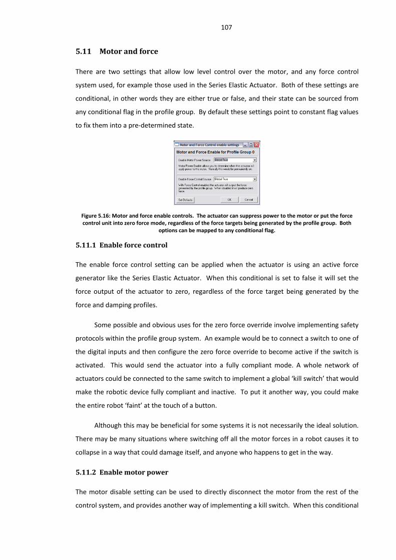
107

5.11 Motor and force

There are two settings that allow low level control over the motor, and any force control

system used, for example those used in the Series Elastic Actuator. Both of these settings are

conditional, in other words they are either true or false, and their state can be sourced from

any conditional flag in the profile group. By default these settings point to constant flag values

to fix them into a pre-determined state.

Figure 5.16: Motor and force enable controls. The actuator can suppress power to the motor or put the force control unit into zero force mode, regardless of the force targets being generated by the profile group. Both

options can be mapped to any conditional flag.

5.11.1 Enable force control

The enable force control setting can be applied when the actuator is using an active force

generator like the Series Elastic Actuator. When this conditional is set to false it will set the

force output of the actuator to zero, regardless of the force target being generated by the

force and damping profiles.

Some possible and obvious uses for the zero force override involve implementing safety

protocols within the profile group system. An example would be to connect a switch to one of

the digital inputs and then configure the zero force override to become active if the switch is

activated. This would send the actuator into a fully compliant mode. A whole network of

actuators could be connected to the same switch to implement a global ‘kill switch’ that would

make the robotic device fully compliant and inactive. To put it another way, you could make

the entire robot ‘faint’ at the touch of a button.

Although this may be beneficial for some systems it is not necessarily the ideal solution.

There may be many situations where switching off all the motor forces in a robot causes it to

collapse in a way that could damage itself, and anyone who happens to get in the way.

5.11.2 Enable motor power

The motor disable setting can be used to directly disconnect the motor from the rest of the

control system, and provides another way of implementing a kill switch. When this conditional

108

is set to false, electrical power will never be applied to the motor, regardless of the state of the

profiles.

Although this can be used to implement a different type of safety protocol than the

system above, it can also be of value with certain specific implementations of actuator

hardware. The prototype actuators being described in this thesis employs a planetary gearbox

to reduce the motor’s speed and increase the torque to a useful level at the output, and as a

result it is possible to back drive the motor by applying a force to the output shaft in order to

manually drive the motor. This relatively low impedance drive is not the only way to construct

an actuator, and it would be equally possible to employ a worm gear that would be impossible

to back drive, or use any other gear system with high impedance. When coupled with the

elastic force sensor any of these drive solutions can be made to behave as a variable

impedance system.

Using active force control lets you vary the apparent impedance of the system by

actively driving the motor in order to maintain a desired deflection within the elastic force

sensor, as a result the system can behave as if it is a variable spring damper, but it does so by

consuming energy. By contrast if we simply replaced the actuator with a real spring, the

system would not require any energy, although we would no longer be able to vary the spring

constant or generate movement in any way.

There are plenty of potential applications where efficient motion can be best produced

with a spring augmented by minimal actuation. These could be in running or hopping tasks,

where certain joints might employ a spring for mechanical energy storage, and an actuator to

add in any energy lost through friction, and to modulate and perpetuate cyclic action. Because

the active force controlled actuator makes use of a spring integrated into the elastic force

sensor, and can employ a high impedance gearbox, it makes sense in some circumstances to

use this spring as a kinetic energy store rather than letting the actuator behave as if it is a

spring, consuming energy in the process.

Equally we can imagine circumstances where we may want to maintain a joint in a

particular position without using energy, for example in a multi legged robot we may want it to

maintain a static stance for a long period without consuming any energy. A high impedance

drive suits this situation, as the joint can remain fixed at around a specified angle without

drawing power, the only movement that will occur within the joint will be that allowed by an

elastic element.

109

The motor power enable setting provides a simple method of implementing these

behaviours when using an actuator with a high impedance drive and active force control. To

give an example, by configuring the motor enable setting to evaluate the state of a threshold

group, and configuring this threshold group to evaluate the force measured by the force

sensor, we can configure a system that will only switch the motor on, and start actively using

the force profiles, when a certain force level has been reached. In this way the system can be

configured to determine when it will make use of the passive springs in the force sensor, and

when it will emulate the spring specified by the force profile.

In actuators without active force control, like the direct drive system, we can use this

mode to switch the actuator into a state that will resist movement by effectively short

circuiting the motor. In these instances the actuator effectively becomes a damper and will

resist attempts to move it.

5.12 External inputs and outputs

The actuator has a number of physical interfaces that allow it to sense and communicate with

the outside world. These are obviously dependent on the specific resources available on the

microcontroller used for the actuator, and for my research I have used two distinct systems so

their differences will be described where appropriate.

5.12.1 RS232 serial communications

The RS232 serial interface provides two functions; these are a method of downloading

configuration data to the device, and a method of exchanging data between devices when

running. Each actuator has a node number for its RS232 communications and will only accept

packets of data destined for that node, except where a packet is marked for node 0. This is

included to ensure that you can establish one-to-one communication with an actuator and

configure it, even if you do not know the node number. Although the RS232 protocol is

designed for point to point communications, this node identifier system has been included

because it is would be possible to change or upgrade the hardware to support a network of

actuators.

In the first version of the actuator the microcontroller had a single serial port interface

and this was used for downloading profile groups and for exchanging data whilst the actuator

was running. In the most current version of the actuator the microcontroller contains a pair of

serial port interfaces but only one of these can be used to download profile groups.

110

5.12.2 Downloading configuration data

The configuration download facility will not be explained in great detail because it is a detail of

the software implementation that does not directly relate to the subject of this thesis. In

simple terms the actuator can accept data for a single profile group at a time, divided up into

seven data packets. These packets contain data for the force profile, the two damping profiles,

the eight bit variable values, eight bit pointer assignments, sixteen bit variables, and sixteen bit

pointer assignments.

When a download is complete the actuator will unpack the data and assign the actual

pointers it is using to the variables specified by the download, before saving all the data to non

volatile flash memory. In addition to downloading up to eight profile groups, an actuator

configuration packet can be sent which specifies which mode the actuator will start in when

powered up (profile control or suspended), which profile group to start with, and the node

numbers for the RS232 communications and the CAN bus if present.

5.12.3 Commanding the actuator

There are a number of serial commands that the actuator will respond to which allow the user

to control basic functions. The actuator has a number of possible operating modes and one of

these is for the profile control system, with another being a default suspended mode. As

already stated, it is possible to configure the actuator to go straight into the required operating

mode when it powers up. Alternatively the actuator can power up into suspended mode, and

a serial command can be sent to switch it into profile control mode (or any other mode built

into the control system). When in a profile group mode the actuator can then be told to

switch back to suspended mode. The profile group that the actuator will start in can also be

configured and controlled by serial commands, so it is possible to tell the actuator to switch

into a particular profile group when it is operating. It is also possible to send a reset command

that forces the microcontroller to restart.

All these commands are made available through the configuration interface so it is

possible to start, stop and reset the actuator by clicking a button on the GUI. A set of sliders

and tick boxes can also be used to send control data, described below, to the actuator.

5.12.4 Exchanging data with the RS232 serial bus

In order to facilitate communication between actuators and other controllers over the serial

bus I have defined a general purpose data packet that can be used for this type of

111

communication. This packet allows an actuator to transmit and receive up to four modulating

variables and four flag variables that, on transmission, are determined by the configuration of

the active profile group, and on reception are immediately available as sources of data for any

of the profile group elements. Each profile group can use two of these data packets, referred

to as group A and B, allowing it to send up to eight variables and eight flags. In the actuator

with a single serial port, both of these packets applied to the single port, but in the latest

version with dual serial ports it is possible to determine which serial port a packet will be

transmitted from. Apart from these details, the way each of these packets work is identical so

I will describe how a single one functions.

When configuring the data packet for a particular profile group the user can, as

illustrated in fig 5.17, select the source for each of the four variables and flags to be

transmitted. Any unused parts are still transmitted and are set to the default zero value.

Figure 5.17: RS232 serial communications. Each profile group can transmit two packets of data per iteration. Each packet is fixed in size, allowing four variables and four flags to be sent. The variables and flags can be sourced from anything visible to the profile group. Timing control can specify that packets are only sent on certain conditions, and specify how frequently packets are transmitted. Actuators can request a reply when

sending packets in order to get data from other actuators.

A condition can be set that determines when the packet is transmitted; this can be

determined by the state of any flag, so when the condition evaluator is set to the global TRUE

flag it will transmit on each iteration of the actuator software. An additional parameter can be

set to make the actuator only transmit once the transmit condition has been met for the

defined number of iterations. For example, setting the auto transmit condition to ON and the

TX Delay value to 10 will make the actuator transmit the data packet every 10th iteration of the

software. In a similar fashion the auto TX condition could be determined by the state of a

112

threshold, in this instance it would only transmit if that threshold has remained active for the

defined number of iterations.

Once the condition for a transmission has been met, the data packet is assembled and

transmitted to the node that has been specified. Each data packet also includes the current

profile group being used, along with the node number for the transmitting actuator and its

current operating mode. The mode would normally only ever be 1 for profile control but it is

included in order to allow the same communication protocol to be used with different

operating modes.

An additional parameter allows you to send a request for a reply along with the data

packet. Any actuator receiving a packet with a reply request will automatically send out a

reply to the transmitting node containing the data specified by the configuration settings for

its current profile group, regardless of whether its auto transmission conditions are met.

Additionally a replying actuator will never request a reply in return, regardless of the

transmission configuration.

On reception of a data packet the control system will extract the values contained in the

packet and place them in a set of variables that the profile group system can use. All incoming

data is stored as variables that are available to all the profile groups, not just the currently

active one.

Because the latest version of the actuator has two serial ports it is possible to configure

one actuator to act like a communications node. With the primary serial port connected to a

controlling computer, and the secondary one connected to another actuator, you can use the

data packet system to route individual variables from one serial port to the other. The speed

at which this data will be passed on is dependent on the settings for the currently active profile

group. Passing on data from one serial port is simply a matter of choosing the incoming serial

variable as the source for the outgoing variable, and it is also possible to send another actuator

a mixture of data from the other serial port, and data about the actuator’s own state. When

configured in this ‘master slave’ relationship you would still want to be able to send low level

commands to each actuator, for example to switch it on or off, so it is also possible to

configure each actuator to pass any of the basic commands, like switching modes or resetting

the CPU, from one serial port to the next. This allows several actuators to be chained together

and to be exchanging packets of data with each other, whilst still allowing a single controlling

computer to start and stop all the actuators at once. What is currently lacking, but would

probably be of value, is some method of downloading configurations to individual actuators

113

within an arrangement like this. Currently the only way to download a configuration is to

connect the appropriate serial port directly to the computer.

5.12.5 CAN bus

The CAN Bus, or Controller Area Network, makes use of a hardware module built into the

microcontroller used in one version of the actuator, and provides the potential for a robust

communication network supporting multiple actuators. Some of the beneficial features of the

CAN system are its speed, operating up to 1Mbps, and its tolerance to noise. It is also

designed as a multi master bus with all the error correction, bus arbitration, and packet

decoding hardware built into the hardware interface. This makes it possible to run multiple

actuators on a single two wire network, each with the potential to communicate with each

other, and any other controllers on the network. Although the configuration interface for the

CAN bus was designed, the underlying code was never implemented and the latest version of

the actuator lacks a CAN module. The explanation of how it works is included to indicate how

this type of bus might be used.

Figure 5.18: The CAN bus. If included a CAN bus can be configured in a similar way to the RS232 serial communications unit. Because it is a network, rather than point-to-point system one actuator can potentially

communicate with many others.

Figure 5.18 shows the configuration options for the CAN bus system and it is very similar

to the RS232 system I have just described. Each profile group has its own configuration

settings and they are divided up into two identical packets, Group A and B. The major

difference between this and the RS232 system is that the user is limited to two variable and

two flags per packet. This is due to the way the standard CAN bus protocol communicates

using packets of eight bytes. Four of these are used to transmit the two sixteen bit variables,

114

with two more for the two eight bit flags. The remaining two bytes are used to transmit

various commands indicating the type of packet being sent.

The CAN Bus has the potential to be used to download actuator configuration settings,

indeed it would be preferable to the RS232 serial bus because the actuator could be updated

remotely over the network rather than requiring a connection direct to the actuator. This

feature has not been implemented yet but is considered an important part of any finished

system.

Figure 5.19 illustrates how both serial communication systems in an actuator with a CAN

bus and RS232 serial interfaces can be used to create complex networks of actuators. It shows

a network of actuators operating on a CAN bus, with some actuators controlling other

actuators over the RS232 serial bus, and other communication links between actuators using

the analogue and digital channels. The flexible packet based communication system allows

actuators to act as simple communication routing nodes, where some data received over the

CAN network can be passed on to the RS232 bus, or data from one RS232 port can be routed

out of the other.

Figure 5.19: Networks of actuators. Illustrating how complex networks of actuators can be constructed using the various communication options available.

5.12.6 Analogue and digital I/O: Details of the non-serial communication options

As described in the section on hardware, each actuator control board has a number of external

connections that the user can access. Currently these consist of a pair of digital input pins, a

pair of digital outputs, a pair of analogue inputs and a pair of analogue inputs.

115

Figure 5.20: Digital and analogue outputs. Both the digital and analogue outputs can be configured for each profile group and, in the case of digital outputs, can be mapped to any conditional flag. Analogue outputs can be

sourced from any system variable and a scaling value allows it to be increased in magnitude.

5.12.7 Digital input and output

The digital inputs provide a source for conditional flags, so a high voltage on a pin represents

TRUE whilst a low voltage represents FALSE. Any element within a profile group that evaluates

flags can use the digital inputs as a source. In order to make the system more flexible the state

of each input pin is copied and inverted to a second flag producing the opposite of the input.

In other words if ‘Digital input 1’ is presented with a positive voltage a variable called ‘ExIn1’

will be set to 1 whilst the variable ‘NOT_ExIn1’ will be set to zero. These flag variables

generated by these inputs can be used for a variety of tasks, one example would be to

configure the motor power enable state to evaluate a digital input, and this could then be

connected to a micro-switch on a joint. When joint passes a limit and the switch is pressed the

actuator’s motor will stop, providing a simple safety mechanism. The status of the digital

inputs is updated on each iteration of the control system.

These inputs are matched by a pair of outputs that can derive their state from any of the

conditional flags in the current profile group. By default they are set to the fixed zero value. A

digital output can, for example, be attached to the flag representing the state of a positive

threshold, so that the output pin will be at zero volts when the threshold is inactive and at five

volts when the threshold becomes active.

5.12.8 Analogue input and output

The analogue inputs can be used to capture real valued signals from external devices such as

sensors. These inputs are captured as a ten bit value before being converted and scaled to a

116

value between -512 and 511. Each value is then available for use within the profile group. For

example the horizontal bias could take its value from one of the two analogue inputs.

To complement the analogue inputs there are a pair of analogue outputs. These can be

configured to take their values from any variable within the profile group, however there is an

additional parameter called the scale. This is a simple integer multiplier that can amplify the

variable to fit within the full range of values that the digital to analogue converter can

produce.

This analogue output scaling is, to be frank, a bit of an ad-hoc solution to a wider

problem with variables within the system. In this particular instance the majority of the

variables tend to work within a range determined by the resolution of the analogue to digital

converter, which generates 10 bit values. These are all scaled to the range -512 to 511. The

digital to analogue converter provides 12 bits of resolution, meaning that a value mapped

straight from an analogue input to the output is effectively scaled down by a factor of four. In

order to get around this I explicitly added in a method of scaling the output variable; however

this problem of variable scales can crop up in other areas and a better solution is discussed in

later chapters.

5.13 Special modes

Whilst the various functions outlined above provide a powerful set of features for configuring

and controlling the compliant behaviour of the actuator, it is unable to produce antagonistic

behaviours that consist of two different spring damping systems working in opposition to each

other, and which are independently controllable. A good example of this is the antagonistic

style actuation found in biology, where groups of muscles which can only exert a pulling force

operate together to control a joint’s motion.

Although it may be desirable to allow the actuator to emulate a biological system, for

example using the ‘Hill type’ muscle model [79], this may require a mode of operation that is

quite specific, and well beyond the range of possibilities that the profile group system is able

to offer. It may be desirable to allow the actuator to approximate some form of antagonistic

actuation using the profile group system and, in order to achieve this, a special mode of

operation involving a pair of profile groups was devised.

117

5.13.1 Profile summation

The profile summation method works with a pair of profile groups at the same time, and sums

their respective force outputs. Figure 5.21, reproduced from chapter three, shows a pair of

profile groups that have been configured to reproduce the behaviour of the simple

antagonistic system described above. In this system each profile group has been given a non-

linear spring at one end of its angle axis such that, when summed together, they produce the

single profile shown at the bottom. By adjusting the horizontal bias for both profile groups

they can be drawn together to restrict the compliant range of the joint, as shown on the right

of figure 5. By adjusting the scale of each profile the stiffness and symmetry of the joint can

also be controlled.

As well as emulating antagonistic joints, the profile summation mode can also be used to

produce other interesting effects. Because the summation applies to the force and damping

profiles in each group it is possible to define one group with a force profile and another group

with a damping profile. Using the same method as above it is then possible to adjust the

relative positions of the damping and force profiles with respect to the angle. By adjusting the

scaling for each it is also possible to individually control the magnitude of spring and damping

forces acting around an equilibrium point.

Figure 5.21: Profile summation. Illustrating how the sum of the outputs of a pair of profile groups can be used to construct antagonistic actuators.

Because the profile summation mode involves two profile groups operating at once, and

because each profile group contains modules that control various elements within the

118

actuator, there is the potential for conflicts when, for example, both profile groups have been

configured to transmit serial data packets. In order to prevent conflicts like this only one of

the profile groups is given full functionality and functions as a ‘master’, with the second profile

group only providing limited functionality.

When the profile summation is enabled it always applies to neighbouring pairs of profile

groups, with the even numbered group acting as the master. In other words profile group 0

can be paired with group 1 with group 0 as the master. All the functions of the master group

are preserved so it has control over serial communications, digital and analogue inputs and

outputs. The slave group can only provide functions related to the force and damping profiles,

so it will only factor in the scaling and biasing modulators when computing an output from its

profiles. Although everything else within a slave group can be configured, only the outputs

from the profiles after biasing and scaling are computed.

The profile summation provides a useful method of adding some of the functionality

described above, but it also has the potential to be significantly improved. Some of these

possible improvements will be discussed in later chapters.

5.14 Profile independent settings

There are a few configuration settings that apply to the actuator as a whole, rather than to

specific profile groups, and although these have been mentioned earlier I will briefly explain

them again for the sake of clarity.

Figure 5.22: Actuator settings. These settings are common to all profile groups.

The first two are the network node numbers or addresses for the two serial

communication settings. These allow the user to give the actuator a unique address for the

RS232 and CAN Bus systems. An actuator address of zero is not allowed, however all actuators

are designed to reply to messages sent to this address. This allows the user to establish

communication with an actuator that has an unknown address (or where the user has

forgotten it) and re-configure it.

119

The remaining two settings are the operating mode and the starting profile. The starting

profile simply determines which profile group the actuator will use when it is powered up,

whilst the operating mode can set the actuator into a variety of different modes. The only two

modes that exist at the moment are mode 0, where the actuator will do nothing except

respond to serial commands, and mode 1 where it will use the profile group system. Other

modes of operation could be included in the future for some alternative control strategies, for

example an explicit emulation of the Hill-type muscle model.

5.15 Execution order

The order in which elements of the profile group are executed during each loop through

the software are as follows:

1. Check both serial buffers and parse the contents if necessary. 2. Read the analogue sensors 3. Read the digital inputs 4. Update the inter-profile communication variables 5. Check to see if profile summation is enabled. 6. Modify the angle using the bias and scale 7. Extract the force and damping values from their arrays 8. Compute the final force value 9. Repeat for the alternative profile if summation is enabled. 10. Check the motor power and force control enable flags. 11. Disable the motor and apply zero force if necessary. 12. Set the force target for the force controller 13. Check the thresholds 14. Check and set the group trigger 15. Set the digital outputs 16. Set the analogue outputs 17. Send serial data packet A and B if required 18. Iterate the oscillator 19. Iterate the profile timer and check its threshold 20. Check the profile switching unit 21. If a switch is demanded change the CurrentProfile variable to the new profile and reset

the timer.

5.15.1 Execution speed

The rate at which a control loop such as the one described above can be closed is an important

factor in the stability and fidelity of any actuator that uses a feedback loop to regulate motion.

An ideal system would allow the loop to close instantly but in reality this is impossible and

some form of delay between sensing the actuators state and generating an output signal is

inevitable.

120

The prototype system I have described was able to close the control loop at a rate of

65Hz. The maximum velocity of the actuator is approximately 1308 degrees per second;

consequently the control system will update every 20 degrees when the actuator is at

maximum velocity. This considerable delay can introduce some stability and fidelity issues

when the system is attempting to approximate spring damping systems that generate high

velocities. Given the way damping and spring forces can be arbitrarily defined across angles it

is entirely possible for the system to skip over, for example, an area of damping that ought to

reduce velocity.

These issues will become apparent in the examples of actuator behaviour detailed in the

following chapter where instability can be seen in systems with large spring and damping

forces that span narrow angles. Understanding these issues is important when trying to create

more stable behaviour and it is possible to calculate a more optimal loop speed.

The hardware imposes a limitation on the number of angles that can be measured. In

our case we have an angle sensor at the output which can measure approximately 300 degrees

of motion and is digitised using a 10 bit analogue to digital converter. This yields a resolution

of approximately 0.3 degrees per bit. A more optimal loop speed would therefore be one that

that, at maximum velocity, updates every 0.3 degrees.

Using the information above on velocity and resolution we can calculate that a loop

speed of 4,360Hz would mean that the actuator can complete an iteration of the control loop

every 0.33 degrees when at maximum velocity. From this we can assume that with an

execution rate of 4.5KHz the system would never skip over any data points on the force and

damping profiles when computing its next force output.

More generally we can use the following equation to determine a minimum acceptable

loop speed for any actuator.

R = ω Q

Where R is the loop speed, ω is the angular velocity in degrees per second and Q is the

sampling resolution in bits per degree.

5.16 Summary

The profile group system as described in this chapter provides some versatile methods of

specifying the actuator’s behaviour in what I hope is a relatively easy to understand, and most

121

importantly, easy to use system. Although the features provide many options for designing

behaviour there will always be times where an extra feature might be useful to generate a

specific behaviour. In the following chapters I will look at the actuator in use, elaborate on

some of the shortcomings of the system, and explore some possible design enhancements that

could be made.

It is worth pointing out that, although the profile group system provides some

sophisticated methods of specifying behaviour, it also preserves the very lowest levels of

behaviour and control. If, for example, the user just wanted to apply a specified force and

read the actuator angle, they can easily configure the actuator to do this. In the case of

generating forces the user can specify a profile group with a uniform zero force profile and

then generate the force they require by applying a vertical bias to shift this zero force line up

or down. If they wanted to control damping then they can also configure the uniform damping

variable to take its value from whatever control variable they desire.

122

Chapter 6

Examples of the Programmable Spring actuator in use

In the previous two chapters I provided details on the electronic and mechanical design of the

actuator, and then the profile group control system that forms the heart of the actuator. The

explanation of the control system provided a few examples of how some of the features might

be used to generate certain behaviours, but only as a method of explaining how these features

worked. In this chapter I will provide a series of examples that demonstrate how the profile

group system can be configured to generate certain behaviours, and provide some data from a

real actuator using these various configurations.

These examples will not only help to illustrate how the various profile group features

can be used to create a number of mechanical effects, but will also highlight some potential

problems with the design. These problems relate both to issues of stability in the system,

particularly when emulating some types of spring system, the fidelity of the system when

trying to emulate certain mechanical properties, and to the limitations of the current control

system.

I will start with a series of simple examples using single profile groups and provide

screenshots from the configuration application illustrating the configurations used. These will

be followed by some examples of multiple profile groups used to create hysteresis, oscillators

and reactive behaviour. Towards the end of the chapter I will provide an example of multi-

actuator configuration illustrating how two or more actuators can be used together to create a

walking mechanism with reflex stepping behaviour.

6.1 Data representations

Throughout these examples I have made use of the force surface visualisations explained in

chapter five. These illustrate the force output of a profile group for every angle and every

velocity, and are presented as a coloured surface where the brightness illustrates the force

magnitude and the colour represents the direction, with red indicating forces pushing the

actuator’s angle down, and blue for forces that will increase the angle. These surfaces are

presented with the angle along the horizontal axis and the velocity along the vertical axis.

123

In order to capture data on the actuator’s behaviour I have made use of the in-built

serial communications system which allows me to output any of up to eight system variables

on every iteration of the control system. A control utility built into the configuration

application allows data to be sent to the actuator using the same packet based system. This

utility can also read incoming data packets from the actuator and log them, allowing variables

like angle and angular velocity to be captured. An additional utility built into the configuration

application can take two of these incoming variables and plot them in real time on the force

surface visualisation as the current angle and velocity, or the profile visualisation as just the

angle. With the force surface this data can be plotted as a point or as a line, and when plotted

as a line the resulting visualisation represents the actuator’s trajectory across the force surface

over time. Where appropriate and useful these visualisations have been captured and are

presented to illustrate the actuator’s behaviour.

Because the serial communications module is used largely for the same purpose

throughout these examples, and for the same purpose between different profile groups, the

configuration application was given an option that allows the settings for serial

communications for one profile group to be replicated across all the other profile groups. This

makes it easy to ensure that, for example, the angle is transmitted as the first variable in a data

packet for every profile group in the actuator, without having to go through each profile group

in turn to set their serial configurations.

6.1.1 Control system speed and power output

The current control system detailed in the previous chapter provides a fair amount of work for

the microcontroller. The majority of the computations are performed on signed sixteen bit

values, but the microcontroller has an eight bit architecture. This produces a control loop that

runs relatively slowly, as a result the profile group control system will complete approximately

sixty five iterations per second. In many respects this is far too slow for what is essentially a

motion control task and some of the effects of this slow update speed, and the resulting

latency between reading sensor inputs and updating its motor output, are manifest in some of

the examples.

Some of these control issues can be addressed easily with faster hardware, particularly

those that relate to the latency between sensing state and computing an output. I will discuss

some of these issues in the next chapter and provide some possible solutions.

124

Although all these examples use the same motor and gearbox combinations, the profile

group configurations could theoretically be downloaded into a different actuator with a

different power output range, but still provide the same functions. When viewing this

research as the basis for an off the shelf hardware component for robot builders it would

probably be desirable for the hardware to be available in a range of form factors and power

outputs to suit different applications.

Because some of these examples are designed to illustrate how the control system can

be used to emulate mechanical behaviour in general, the values for force and velocity are kept

in the range of values as captured by the hardware, and do not directly relate to any absolute

force or velocity. The details of the hardware in chapter 4 provide an indication of the range of

torques and velocities that the prototypes used here can generate. The maximum speed of

the output is approximately 218 rpm or 1308 degrees per second whilst the maximum (stall)

torque is 0.748 newton meters. Roughly speaking for the measurable velocity range of -512 to

511, the actual motor can generate (without any opposing or assisting forces) a maximum

velocity that covers 80% of this range. The angular range is approximately three hundred

degrees and is confined by mechanical stops; however it is possible with one version of the

hardware to use the controllable voltage references to tune the measured angular range to

the mechanical one. This means that for an actuator with a mechanical range of two hundred

degrees it is possible to configure it so that the full range of angles that the hardware can

measure will match the range of angles that it can actually achieve.

For the sake of simplicity then the configuration application and its visualisations are not

related directly to real angles, torques or velocities but to the values captured by the

hardware. If this system were to be developed beyond this thesis, and actuators with a range

of different performance characteristics developed, then it would be more sensible to provide

real values for these graphs that relate to the particular actuator being configured or

controlled. When comparing the actuator behaviour to a real mechanical system the

actuator’s electronic hardware is used to capture this data from the angle sensor, and so it is

presented in exactly the same format, and at the same scale, as data from a complete

actuator.

6.1.2 Experimental setups

There are a variety of different examples here which require the physical actuator to be

mounted in certain ways and with certain attachments. For the simple examples at the start of

the chapter the actuator has been fitted with a lever on its output shaft to turn the actuator

125

into a mechanical joint. This lever also contains a small mass. To demonstrate some

behaviours the actuator is mounted so the lever’s movement is horizontal with respect to

gravity – in other words it is unaffected by gravity regardless of its angle – and the lever is then

manually deflected and released to demonstrate the effects of the profiles on its movement.

6.2 Simple spring damping systems and modulators

The first set of examples will look at configurations using single profile groups to produce

spring like behaviour, and then spring damping behaviour. This will be followed by an example

of biasing and scaling applied to the profiles. The early examples deal only with spring

behaviour. Because of their simplicity they provide an opportunity to compare the actuator’s

behaviour to a real system. For later behaviours, particularly those involving complex spring

dampers, it was considered too complex, time consuming, and of too little value to try and

construct mechanical equivalents of the behaviours being produced. Two examples of

mechanical spring systems, and how the actuator can emulate them, are presented first and I

will discuss the results of these demonstrations before moving on to more complex examples.

6.2.1 Linear and non-linear springs

The first few examples deal with simple springs and demonstrate how the actuator can

reproduce the behaviour of a toy mechanical system. For these examples I have produced two

different, purely mechanical sprung joints, and then configured the actuator to reproduce the

behaviour of the mechanical equivalent. For these first examples I have used two different

versions of the actuator, the direct drive system and the version with the Series Elastic

Actuator force control. To produce the mechanical versions of these examples I have used an

existing actuator, but removed the motor to create a passive rotary joint. The angle sensor

and control circuit are left in place and are used to capture data.

The first system is a simple pair of linear extension springs that create an equilibrium

point in the centre of the actuator’s range of motion. The extension spring had a rate of

approximately 2 newtons per centimetre and the spring would extend or contract by 3 cm over

an angle of ninety degrees. The mechanical version of this system is shown in figure 6.1, along

with a schematic representation. A pulley wheel was attached to the actuator’s output and a

cable wrapped around this was terminated at each end by an extension spring that attached to

the actuator’s body. This had the effect of holding the output at an equilibrium point between

the springs.

126

Figure 6.1: A pair of linear mechanical springs.

To recreate the behaviour of this sprung joint with the actuator I created a simple linear

force profile with an equilibrium point in the centre of the angular range, as shown in figure

6.2. This was configured with the application software, using the ‘point to point’ function, to

draw a force line from a force value at the start of the angle axis to an opposing force value at

the end of the angle axis. This should create the effect of a pair of springs, with an equilibrium

point in the centre where the force line crosses zero on the vertical axis.

Figure 6.2: A linear spring profile designed to match the mechanical equivalent.

This configuration was downloaded to the actuator, and also to the controller in the

mechanical equivalent.

The actuator and its mechanical equivalent were mounted on a bench so that the levers

attached to their outputs could move horizontally. Both levers were then manually deflected

away from their equilibrium points by ninety degrees before being released. The resulting

behaviour was captured, and is shown in figure 6.3. As can be seen there are some

discrepancies between the rate at which the mechanical system oscillates and the emulated

system. With the direct drive system this is to be expected because we are just setting the

voltage of the motor. Although this will translate into torque in a reasonably linear fashion,

this is only true when the motor is stationary, so as the velocity increases so the applied torque

will decrease. The motor itself is capable of driving an oscillation at the same rate as the

mechanical spring, but to do so it would require either some active control of the torque,

127

based on the motor’s current consumption, or some other control scheme that compensates

for the drop in torque as the velocity increases.

Figure 6.3: A linear spring profile compared to a mechanical equivalent. The force surface trajectories for each system are shown below the graph.

I should point out that these results were obtained after some tweaking of the force

profile used in the actuator. Although the spring values of the mechanical system were

known, the profile system does not yet allow you to specify forces in proper terms (as

newtons). In order to determine what values to specify in the profile, the mechanical spring

system was connected to an actuator and a force value applied with increasing magnitude

until the lever became deflected by ninety degrees. In other words the real and the virtual

springs cancelled each other out. This was then used to determine the maximum value at each

end of the force profile.

The second mechanical system shown in figure 6.4 involves creating an equilibrium

point between two non linear springs, and this is achieved by attaching a single extension

spring to a short lever on the rotary output of the passive actuator, with the other end of the

spring attached to the actuator’s body. The extension spring had a rate of approximately 5

newtons per centimetre and the length difference between its resting position and its

extended position when the lever was at ninety degrees was approximately 2cm. When the

output is deflected away from the centre angle the spring is pulled, and because of the

changing mechanical advantage that the short lever exerts as it rotates, the extension of the

spring becomes non linear with respect to the angle.

128

Figure 6.4: A pair of simple non-linear mechanical springs.

In order to reproduce this spring system with the real actuator I used the profile

generator tool in the configuration application to generate the force profile shown in figure

6.5. This used the sine function, and a facility to mirror it horizontally and vertically to produce

a symmetrical spring profile.

Figure 6.5: A non-linear spring profile designed to match the mechanical equivalent.

As with the previous experiment, the outputs of the actuator and the mechanical

equivalent were deflected away from their resting positions by ninety degrees and then

released. The resulting angle and velocity data was captured and is shown in figure 6.6. As

with the previous example a certain degree of tweaking was required in order to find the

correct profile to match the mechanical system.

Figure 6.6: A non-linear spring profile compared to a mechanical equivalent.

The results of the linear and non linear spring behaviours are not great. The Series

Elastic Actuator appears marginally better than the direct drive system but neither is able to

129

reproduce the behaviour of the real springs. Both devices are producing behaviour that is

more like a damped spring. In the case of the direct drive system this performance difference

is to be expected because the motor and gearbox produce a damping effect, and the motor’s

inertia, amplified by the reduction gear, also has an effect on its behaviour. With the Series

Elastic Actuator version the performance is disappointingly poor, but some of this can be

accounted for by the low fidelity and poorly tuned hardware I am using. These performance

issues will be discussed in more detail in the next chapter.

6.2.2 Simple linear springs with damping

The next three examples show how damping can be added to control the behaviour of simple

spring systems. The first example takes the simple linear spring from above, and adds

damping to prevent the spring like oscillations it produces. The second two examples look at a

single spring at one end of the range of motion, firstly with normal conditional damping and

secondly with inverse uniform damping.

The goal with this first example is to replicate, in a crude fashion, the behaviour of a

position control system where we want to cause the actuator’s output to return to the

equilibrium point after being deflected away, but without the oscillations caused as the lever

overshoots the equilibrium point. In order to achieve this we want damping to be applied so it

will arrest the motion of the actuator as it approaches the equilibrium point. Normally with a

position control system the degree of damping will not change with respect to the angle, so to

model this we can specify a level of uniform damping that covers all angles; however with

many position control systems the intention is to get the output to return to an equilibrium

point as fast as possible, so if we apply damping across all angles then we may end up reducing

the velocity of the output at angles where we should actually be generating maximum velocity.

Figure 6.7 shows a simple linear spring profile, but with damping added for each

direction of motion. The force surface that results from this damping is also shown on the

right. In order to produce a system that maintains a degree of compliance, but prevents the

oscillations, I have defined damping that applies only at angles closest to the equilibrium point,

and which rises in magnitude as the angle approaches this point. This is achieved by drawing

damping profiles that rise to a peak at the equilibrium point so that the system has the highest

level of damping at this point.

130

Figure 6.7: Creating a damped equilibrium point. The force surface on the right represents the angle along the X axis and angular velocity on the Y axis.

I was not able to replicate this in a purely mechanical system due to the complexities of

creating the variable dampers, but the experimental procedure was the same in that the

output lever was deflected to ninety degrees and released. The behaviour is recorded in figure

6.8 and includes a plot of the actuator’s trajectory across the force surface.

This is not intended to replicate a high accuracy position control system but, as the

results show, the conditional damping can be used effectively to control the motion of the

actuator and prevent oscillations, whilst maintaining compliance.

Figure 6.8: A plot showing the angle over time as the lever is deflected away from its equilibrium point and released. The inset illustrates the trajectory across the force surface. The lever was deflected and released once

in each direction.

When compared to many traditional position control algorithms there is one element in

my control system that is missing. Whilst it is easy to use the spring and damping profiles to

produce the equivalent of a PD (Proportional Derivative) controller, there is no way of adding

an integral term in order to create a PID controller. There may be no real reason to do this, as

this system is not an attempt to recreate traditional motion control algorithms, but this will be

discussed in the next chapter.

131

The next example reproduces the effect of a spring damper at one end of the actuator’s

range of motion and is designed to prevent the actuator moving beyond a certain position.

Figure 6.9 shows the force and damping defined for this experiment and the resulting force

surface. I have only defined damping to apply in one direction of motion so it will affect the

output when it is moving against the virtual spring, but not when the spring is pushing it back.

Figure 6.9: A unidirectional damper and spring.

For this experiment the actuator is mounted vertically so that the output lever can be

lifted up and dropped to fall against the spring dampers under the pull of gravity. A second

test involved depressing the lever against the virtual spring and then releasing it. The two

resulting behaviours are plotted in figure 6.10.

The effects of the conditional damping are evident in the way the motion of the lever

when dropped is arrested quickly with little bounce back produced by the spring, but when the

lever is pressed against the spring and released it does bounce up before falling back and being

halted by the damper.

Figure 6.10: Two plots of the actuator’s trajectory across a force surface. On the left the trajectory shows how the lever behaves when it is dropped against the springs. On the right the lever is pushed against the springs before

being released.

In the final example I have removed the damping from the previous one and instead

applied a small uniform damping level of -1. This damping applies across all angles and

directions, and I have specified a low negative value. This has the effect of reducing the

influence of friction on the system so with the right amount of damping the system should

behave as if some components of friction, those produced by viscous damping, have been

132

removed completely. As before, the lever is dropped against the virtual springs and the output

behaviour is captured and plotted in figure 6.11.

Figure 6.11: A single spring with inverse damping. The lever is dropped against the spring and bounces back producing a continuous loop.

As can be seen the lever bounces perpetually against the spring, behaving as if there is

no friction to slow it down.

6.2.3 Modulating springs and dampers with the bias and scale

The next set of demonstrations illustrates the use of the bias and scale modulators on some

simple spring damping systems. To start with I have taken the simple damped linear spring

example illustrated in figure 6.7 and configured the profile group to allow me to set the

horizontal scale with a serial control variable sent from the configuration application. I have

also created an identical system but with the damping removed. The horizontal bias is also

configured to take its value from the internal oscillator, which is set to produce a value that

varies between -200 and 200, with the step size set to 8, and prescaler to 1. This produces an

oscillation of approximately 1.5Hz. The actuator is mounted so its output is not affected by

gravity. Sourcing the horizontal bias from the oscillator has the effect of moving the springs

and spring dampers in the two examples along the angle axis, causing the output lever to keep

chasing a constantly changing equilibrium point. The horizontal scale is kept at a fixed value of

1.0 for the first experiment. The results of both the damped and un-damped systems are

shown in figure 6.12.

In the second example I have added a variable horizontal scale value to the previous

experiment. The actuator begins with a scale value set to zero and this is slowly increased by a

value of two, approximately five times per second, until it reaches a value of 500. The result is

to slowly increase the strength of the springs from zero up to a reasonably high value. In the

case of the damped system, the angular range of the damping is reduced as the scaling

increases, but the magnitude remains the same. The scale value of 500 being sent to the

actuator represents an actual scaling of 5.0, so the result, in terms of the way the software

133

works, is to multiply the apparent angle by 5 before looking up the force and damping values

in the profile data arrays.

Figure 6.12: Angle plots for two linear spring profiles, one with and without damping, being biased along the angle axis by an oscillator.

The outputs of both systems are shown side by side in figure 6.13. As can be seen the

systems start by producing no movement, and as the scale value increases they begin to track

the changing equilibrium points more aggressively, before starting to become unstable as the

spring constants increase to their maximum. The plain spring profile produces a much more

unstable behaviour earlier on, but this is simply re-creating the ‘wobble’ seen in the

experiment with a fixed scale above and is to be expected from a system that is, in essence, a

mass, coupled to an oscillating actuator, by a spring. The damped system shows a much more

stable behaviour which tracks the moving equilibrium point smoothly over a range of scales,

but as it approaches higher scales the behaviour begins to show some instability.

The principal reason for this instability is the latency and speed of the control loop.

Because the actuator is capable of moving its output at high speed, and the control loop

operates at a rather slow 65Hz, the output can end up travelling a fair distance between

updates. When the spring forces are high, and the slopes that cross equilibrium points are

steep, it is possible for the actuator to travel from one extreme of force to another without

registering the zero force equilibrium point in the centre. The result is an oscillator that

bounces between these two high force points. Because of the way damping has been defined

across a narrow range of angles, close to the equilibrium point, the scaling has the effect of

making this damping range even narrower. This reduces the damping effect and, due to the

134

problem of control loop speed, increases the chances that the actuator will skip across this

damped region during each iteration, removing damping altogether.

Figure 6.13: Angle plots for plain (top) and damped (bottom) linear spring profiles as their horizontal bias is oscillated and the scale slowly increased.

6.2.4 Some issues with profile based damping

Some interesting issues arise when the biasing of a profile is compared to the more

conventional computed spring damper or mechanical equivalents. At the core of the issue is

the fact that damping is applied to the motion of the actuator’s angle. If we take the example

of COG’s arm from chapter three, where a Proportional Derivative (PD) controller was used to

create a spring damped joint, some interesting differences come to light.

The control system used in COG’s arm relied on a force generating actuator with an

angle sensor in the joint. To create a sprung and damped joint, a control system used an angle

set-point and compared it with the actual angle to generate an error value. This error value

was then multiplied by a constant to generate a spring force, and the error velocity was also

multiplied by a constant to produce a damping force. The sum of these two values was then

applied to the force generator. Although the traditional purpose of a PD controller is to

generate rigid position control by ironing out deviations from a desired angle the application of

this control strategy to a force controlled actuator can produce an approximation of a

compliant mechanism with independent control over the spring and damping forces that

define the compliant behaviour, and which can be used to generate useful behaviour, as

135

demonstrated with the crank turning experiment discussed in chapter three. In this instance

the effect is to produce a sprung and damped joint with an equilibrium angle specified by the

set-point.

With this system the damping is not directly a product of the angular velocity but

instead it is computed from the error signal. If we were to introduce a change in the set point

then the error, and consequently the error velocity, would also reflect this change. The effect

of this would be that sudden changes in the set point would result in large forces at the joint as

the sudden increase in error velocity produced a high damping force in opposition to this

apparent movement.

With the profile system the effect is very different. Here we have a bias instead of a set

point, but we are still able to introduce step changes and instantly shift the bias around.

Unlike the previous example, our damping is directly tied to the angle velocity, and as a result

step changes in the bias will produce no change in the velocity signal. The damping specified

for the joint will only begin to come into effect when the joint begins to move.

In order to illustrate this better, consider the following two spring damping systems

illustrated in figure 6.14. Here I have drawn them as linear mechanical systems but the point

applies equally well to a rotary joint, it is just easier to represent in linear form. Both examples

are of a system with an equilibrium point held between a pair of springs. The other ends of

the springs are attached to a linear actuator allowing the springs, and the resulting equilibrium

point, to be moved about.

Figure 6.14: Comparing the effects of damping. A virtual spring damping system based on set-points and errors is equivalent to the first mechanical system (A) where the springs and dampers are parallel and affected by

movement in the actuator or the output. The profile based spring damping is more like the second system (B) and has a damper that is only affected by movement of the mechanical output.

The first example contains a damper connected in parallel with the springs. This is

mechanically equivalent to the PD controller in COG’s arm in the way that any change in the

input position of the actuator will affect the damper as well as the springs.

In the second example I have moved the damper so it is connected to the output of the

system. With this system a change in the position of the actuator will alter the spring tension

136

but the damping will only come into effect when the joint begins to move. This system is

analogous to a linear spring profile with a specified level of uniform damping that applies

across all angles, or identical damping profiles that are uniform across all angles.

Both of these examples are mechanically valid, however the first example cannot be

reproduced with my control system. This is probably easy to fix by generating a velocity

variable from horizontal bias, and allowing this to be summed with the angle velocity when it is

used to compute the damping forces. This and other issues relating to the way the system can

emulate mechanical spring damping assemblies are important, and I will re-visit this topic in a

bit more detail in the next chapter.

6.3 Latches, oscillators and multi-profile systems

The first set of examples illustrated how various spring damping behaviours can be created

using the profiles for force and conditional damping, and how the scale and bias can be used to

control equilibrium points and spring constants. In this next section I will show how multiple

profile groups with conditional switching can be used to create more complex mechanical

behaviour.

6.3.1 A simple latch with hysteresis

In chapter three I explained how a pair of profiles with angle thresholds could be used to

create latching behaviour. This next example demonstrates this latching system, and how

pairs of profile groups are used to create it.

Figure 6.15: Creating a latch. The two profile groups are mirror images and the actuator will swap from one to the other when a threshold is passed.

Figure 6.15 shows a pair of profile groups, each configured with linear spring systems

that produce an equilibrium point towards one end of the range of motion. The two profiles

are mirror images of each other with respect to the behaviour they generate, and each also

has a threshold set to check the angle. The threshold for each is towards the strong end of its

spring, so the force will tend to push the output away from the threshold. The profile

137

switching unit for each profile group is set to evaluate its threshold and, if active, will switch

over to the other profile group. The arrows in figure 6.15 illustrate how the thresholds will

cause the system to jump to the alternate profile group.

To demonstrate this system in action I mounted the actuator horizontally, and manually

deflected the lever away from one equilibrium point until it latched into the alternate position.

I then manually returned the lever to its original position. The output angle was captured

along with the force output, as specified by the force profile, and the data is shown in figure

6.16.

Figure 6.16: Latch behaviour. A graph of angle and force against time as the latch is manually moved from one position to the other.

6.3.2 Turing a latch into an oscillator

The latch with hysteresis can very easily be converted into an oscillator. Figure 6.17 illustrates

a slightly modified pair of profile groups designed to produce an oscillating output. The two

main alterations are that the springs have been altered to push their equilibrium points further

towards the end of the profile, and their thresholds have been changed so that they are now

at the other ends of the springs, just before the equilibrium points. Each profile will now tend

to push the output towards the threshold which, when triggered, will jump to the other profile

group.

Figure 6.17: Creating an oscillator. The two profile groups are identical to those used for the latch but the angle thresholds have been switched to create an oscillator.

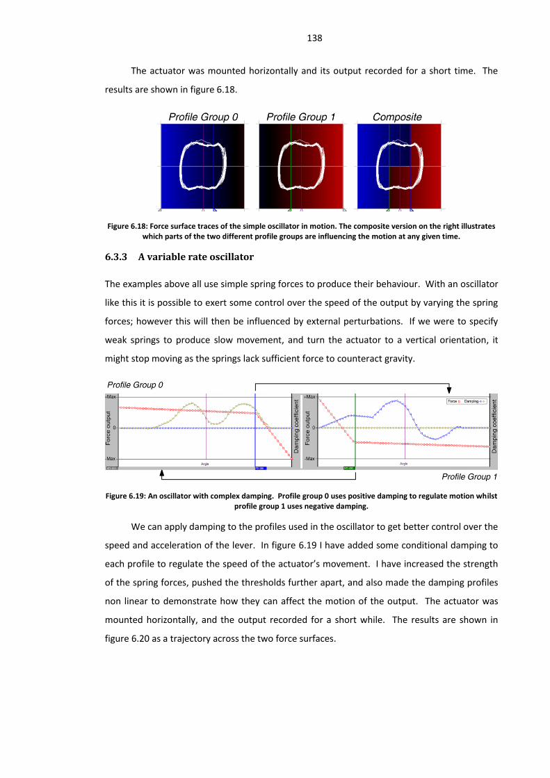
138

The actuator was mounted horizontally and its output recorded for a short time. The

results are shown in figure 6.18.

Figure 6.18: Force surface traces of the simple oscillator in motion. The composite version on the right illustrates which parts of the two different profile groups are influencing the motion at any given time.

6.3.3 A variable rate oscillator

The examples above all use simple spring forces to produce their behaviour. With an oscillator

like this it is possible to exert some control over the speed of the output by varying the spring

forces; however this will then be influenced by external perturbations. If we were to specify

weak springs to produce slow movement, and turn the actuator to a vertical orientation, it

might stop moving as the springs lack sufficient force to counteract gravity.

Figure 6.19: An oscillator with complex damping. Profile group 0 uses positive damping to regulate motion whilst profile group 1 uses negative damping.

We can apply damping to the profiles used in the oscillator to get better control over the

speed and acceleration of the lever. In figure 6.19 I have added some conditional damping to

each profile to regulate the speed of the actuator’s movement. I have increased the strength

of the spring forces, pushed the thresholds further apart, and also made the damping profiles

non linear to demonstrate how they can affect the motion of the output. The actuator was

mounted horizontally, and the output recorded for a short while. The results are shown in

figure 6.20 as a trajectory across the two force surfaces.

139

Figure 6.20: Force surface traces of the complex oscillator in motion. The composite version on the right illustrates which parts of the two different profile groups are influencing the motion at any given time.

It would also be possible to control the overall oscillator rate by adjusting the uniform

damping variable. This will affect the motion of the actuator across all angles and directions,

and works on top of the conditional damping.

6.4 Reactive behaviour

The examples above can be extended to produce much more complex latching and oscillating

systems by adding extra profile groups to the system. By adding new profile groups to the

latching system, and modifying the profile switching units so that these new profile groups are

selected when the right thresholds are passed, it is possible to create a latch that will progress

through multiple states during operation. In a similar fashion we can add more profile groups

to the oscillator example above and produce a system with behaviour that varies across

several oscillations.

It is also possible to combine oscillating and latching systems to produce a number of

intermediate behaviours. We can create a latch that will produce a series of movements when

it is operated before returning to its starting state, or we can produce oscillators that can be

manually halted by introducing stable equilibrium point that would normally be overshot

during oscillations, but can be found when an external force intervenes.

In order to better demonstrate how these multi-state systems can be created and used,

I have used the example of a pin-ball flipper for the following demonstrations. The actuator

has been fitted with a long lever arm on its output shaft, and mounted on the ground so the

lever arm can move horizontally, as shown in figure 6.21. The idea is to create a set of

behaviours to control the actuator so it can react to a ball making contact with the lever. I

have produced a series of examples starting with a simple reactive flipper that uses springs

only and moving on to add damping in order to refine the behaviour. The final example shows

how profiles can pass state information to each other in order to create a flipper with a

response that is dependent on the speed of impact.

140

Figure 6.21: An actuator fitted with a pin-ball flipper arm alongside a large plastic ball.

In all these examples the actuator is tested by rolling a large ball against the lever in

order to trigger the behaviour.

6.4.1 A simple two state pinball flipper with no damping

This first simple example uses two profile groups and two angle thresholds in each to make a

reactive lever. Figure 6.22 shows the two profile groups used. The system begins with group

0, where it has an equilibrium point with a strong linear spring on one side and a weak

constant spring on the other. The threshold is set to trigger when the lever is pushed against

the strong linear spring and, when passed, the actuator will jump to profile 1. In this profile

there is a strong constant spring that drives the lever in the opposite direction towards

another threshold. When this threshold is passed, the actuator returns to profile 0, where the

weak constant spring will return the lever to the equilibrium position.

Figure 6.22: Two profiles used to create a reactive pin-ball flipper.

141

A plot of the actuator’s angle against time is shown in figure 6.23. Although it appears

to work, in reality it took some careful tuning of the spring forces in profile 0 in order to

prevent the actuator from overshooting the equilibrium point and triggering itself again after it

had flipped the ball. To prevent this self triggering problem I had to specify fairly strong spring

forces against which the ball had to push before the flipper threshold was reached, which in

turn meant that I had to roll the ball fairly hard against the lever before it worked. Even with

this careful tuning it would occasionally trigger itself anyway, and it also takes some time to

settle.

Figure 6.23: A plot showing the pin-ball flippers angle against time as a ball is rolled against it. The two lines A and B show where the two angle thresholds are.

6.4.2 Adding damping to refine the behaviour

In order to refine the behaviour from the first example, and make the flipper more sensitive to

perturbations, I added some damping. The resulting configuration is illustrated in figure 6.24

and shows how conditional damping has been applied to both profile groups. In profile group

0 the spring on one side of the equilibrium point has been weakened, and the threshold

moved closer in order to make the device more sensitive. To prevent overshoot I have added

damping along the weak constant spring that peaks as it approaches the equilibrium point, and

I have also increased the strength of the spring in order to get the lever to return to this point

faster. This damping only applies when the lever is returning to this equilibrium point. In

profile group 1 I have added some damping that applies as the actuator reaches the other

angle threshold so that the lever will have begun to slow down as it passes this threshold.

142

Figure 6.24: A pin-ball flipper with damping. Damping for certain angles and directions of motion has been added to provide more control over the flippers behaviour. The inset images show the force surface produced by each

profile group.

Rolling the ball against the lever produces the results shown in figure 6.25. As can be

seen the behaviour is much improved in the sense that the lever is triggered more easily, and

returns to its resting position much more quickly than before.

Figure 6.25: The behaviour of the damped pin-ball flipper as a ball is rolled against it. An inset shows the flippers trajectory over a composite of the two force surfaces as the ball is rolled repeatedly against the flipper.

6.4.3 A velocity dependent flipper

The previous two examples both react by flipping the ball with the same amount of force, so in

this next example I have modified the configuration so that the force used to push the ball is

partly dependent on the velocity of the lever when the threshold was passed. The intention is

to create a system where the flipper will respond gently when the ball strikes it gently, but

with greater force when it strikes hard.

In order to achieve this I need some method of saving the angle velocity from when the

triggering threshold was reached in profile group 0, and using it to modify the spring force

used in profile group 1. Saving this velocity value can be achieved by using the inter profile

variables. As explained in the section 5.9.2 of the previous chapter, these are variables that

belong to each profile group, but are visible to all other profile groups, so we can configure

one of them to source its value from the angle velocity of profile 0, and then use this value in

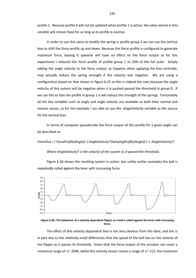
143

profile 1. Because profile 0 will not be updated when profile 1 is active, the value stored in this

variable will remain fixed for as long as its profile is inactive.

In order to use this value to modify the spring in profile group 2 we can use the vertical

bias to shift the force profile up and down. Because this force profile is configured to generate

maximum force, biasing it upwards will have no effect on the force output so for this

experiment I reduced this force profile of profile group 1 to 20% of the full scale. Simply

adding the angle velocity to the force output, as happens when applying the bias vertically,

may actually reduce the spring strength if the velocity was negative. We are using a

configuration based on that shown in figure 6.25 so this is indeed the case because the angle

velocity of this system will be negative when it is pushed passed the threshold in group 0. If

we use this to bias the profile in group 1 it will reduce the strength of the springs. Fortunately

all the key variables such as angle and angle velocity are available as both their normal and

inverse values, so for this example I am able to use the -AngleVelocity variable as the source

for the vertical bias.

In terms of computer pseudocode the force output of this profile for a given angle can

be described as:

ForceOut = ( ForceProfile[Angle]+ ( AngleVelocity*DampingProfile[Angle]) ) + -AngleVelocityT;

Where AngleVelocityT is the velocity of the system as it passed the threshold.

Figure 6.26 shows the resulting system in action, but unlike earlier examples the ball is

repeatedly rolled against the lever with increasing force.

Figure 6.26: The behaviour of a velocity dependent flipper as a ball is rolled against the lever with increasing force.

The effect of this velocity dependent bias is not very obvious from this data, and this is

in part due to the relatively small differences that the speed of the ball has on the velocity of

the flipper as it passes its threshold. Given that the force output of the actuator can cover a

numerical range of +/- 2048, whilst the velocity sensor covers a range of +/- 512, the maximum

144

amount of bias that can therefore be applied to the force will only reach 512 in extreme

circumstances. The velocities generated in the example here only covered a range of about

120, which is less than ten percent of the full force range of the actuator. Without an in-built

method of scaling this velocity signal up to a more useful value, the effect it has on the flippers

response to the ball will always be small. This deficiency in the control system with regard to

the way variables can only be mapped directly to other variables, without any scaling, is

something I will discuss in more detail in the next chapter.

6.5 Robotic legs

The final set of examples take a more practical approach to look at how these actuators can be

used to construct robotic systems with useful properties. I will show how actuators in a simple

pair of legs for a walking robot can be coupled together mechanically and electronically to

produce a single leg with an in-built stepping reflex and a pair of legs that co-ordinate their

stepping behaviour.

Unfortunately there were not enough prototype actuators constructed to make a fully

articulated walking robot, so the system demonstrated here uses only two legs, with a set of

wheels to support the rest of the body. The principle being demonstrated here can be

expanded to accommodate more legs.

6.5.1 A two degree of freedom leg with a stepping reflex

The basic leg joint consists of two actuators, one knee actuator to lift the leg up and down and

one shoulder actuator to swing it forwards and backwards. The basic mechanical arrangement

of the leg, and a pair of legs connected to produce a simple walking mechanism, is shown in

figure 6.27. The walking mechanism included a set of stabiliser wheels to prevent the robot

from toppling over, and remove the need for it to perform the much more complex task of

balancing. Because the actuators produce a relatively low level of torque, but are also fairly

heavy, the knee joints were not powerful enough to overcome the mass of the robot. A

counterweight was added to the rear of the robot which reduced the apparent weight of the

robot for the knee actuators.

For the knee actuator that lifts the leg I have defined a force and damping profile that

presents a strong spring, with some damping to support the robot’s body, and a weaker spring

on the other side of an equilibrium point that prevents the leg dropping too far when it is not

supporting any weight. For the shoulder actuator that will allow the leg to step I have defined

a symmetrical sprung joint, with a small degree of damping, to create an equilibrium point

145

where the joint will want to rest. I have also given this joint a pair of angle thresholds on each

side of the equilibrium point.

Figure 6.27: A two degree of freedom leg joint (right) and a pair of legs connected together (left) to create a simple walking mechanism. Underperformance of the actuators in terms of torque limits necessitated the

inclusion of a counterweight to reduce the weight that the knee actuators were required to lift. A set of stabiliser wheels prevent the robot from falling and a wheel at the end of each leg served to reduce friction when the knee

actuators lift the robot’s body.

These configurations create a leg that will, when combined with other legs, maintain the

robot’s body in a stable static stance. In order to get a leg that can react to perturbations, by

stepping forwards or backwards, we can add a few extra profile groups to each actuator and

get them to co-ordinate each other’s actions.

The thresholds defined for the shoulder actuator can be used to trigger the stepping

behaviour. When the robot is standing, the springs in this actuator should keep it stable, but if

the robot is pushed with enough force then the threshold will be passed as the robot’s leg gets

deflected relative to its body. When this happens we want the leg to lift off the ground and

move in the direction that the robot’s body is being pushed. To achieve this I have configured

the shoulder actuator to activate a digital output when either of its thresholds is passed. The

digital output is then linked to the digital input of the knee actuator, which is configured so

that, if its digital input becomes active, it will switch to an alternate profile designed to lift the

leg.

This alternate profile remains active for as long as its digital input is active, so the

moment the threshold in the horizontal actuator is no longer passed, the vertical actuator will

drop the leg back down to its original position.

146

Although this configuration is nice and simple, and appears to be functional, a quick test

of the leg revealed a slight flaw. When the leg lift is triggered by the threshold, the release of

the leg from contact with the ground allows the springs in the vertical actuator to begin

moving it back towards the equilibrium position, and it immediately falls back inside the

threshold, which in turn drops the leg onto the ground. Although this produces the correct

type of action the movement happens so fast that the leg does not have enough time to step

very far. What I really want is for the leg to return to its horizontal equilibrium position, or

perhaps even go past it in anticipation of more movement of the body in that direction.

In order to get this behaviour I have to add a slightly more complex set of profiles to the

shoulder actuator. The two thresholds now both trigger a jump to a pair of different profile

groups, one for each threshold. Both of these profile groups contain a similar, but stronger,

sprung equilibrium point, and will activate a digital output to signal to the other actuator to lift

the leg. These two profiles also contain a threshold set close to the equilibrium point, but

working in the opposite direction, and in each case when the threshold is passed it will return

to the original profile group. The purpose of these two thresholds is to tell the leg that it can

drop back down when it has returned to its horizontal equilibrium point, but it is necessary for

me to use two different profile groups here because we want the leg to produce the correct

behaviour when stepping forwards and backwards.

Figure 6.28: The shoulder actuator’s three profile’s on the left, and the knee actuator’s two profiles on the right. The knee actuator’s active profile is determined by the shoulder actuator so that, when the ‘Shoulder Normal’

profile is active, the ‘Knee Down’ profile is also active, and when either of the ‘Shoulder Back’ or ‘Shoulder Forwards’ profiles are active, the ‘Knee Up’ becomes active.

This new mechanism works much better and the leg will produce reasonably good reflex

stepping movements in response to perturbations. The profiles used for both actuators, and

their switching relationships, are shown in figure 6.28 and the behaviour of the leg, in terms of

the changing angles of the shoulder and knee joints as it takes two steps forward, is shown in

figure 6.29. Data from the knee joint was not captured directly, but passed using the serial

communications system to the shoulder actuator, before being transmitted and logged.

147

Figure 6.29: Angle data from the shoulder and knee actuators in a leg as it reacts to a perturbation by stepping forwards.

6.5.2 Coupling a pair of legs for coordinated reflex stepping

With a pair of the legs described above, and a supporting mechanism to prevent the robot

falling over, we should be able to make a simple walking system that will walk in the direction

it is being pushed. There is one thing we need to consider though before this is implemented –

what will happen if both legs try to step at the same time? The answer should be obvious in

that the robot will fall over, so we need to devise some mechanism to prevent both legs being

triggered at the same time. To do this we can make use of the way that the threshold system

has an enable parameter for each threshold in a group, and this allows us to switch on and off

a threshold in a profile group. By using this feature, the thresholds that control the stepping

behaviour can be configured to deactivate if a digital input becomes active, and we can then

use the digital output of an actuator in one leg to suppress the stepping action in the other leg.

The result should be a system where the first leg to pass its threshold will take a step, and the

other will take its turn after the first one has completed its step.

When this is implemented we have a simple robot that can automatically take a step

when it is pushed forwards or backwards. To test the robot it was pulled along with a

makeshift leash, and the stepping reflexes in both legs worked to keep the front of the robot

supported off the ground. Capturing reliable data from all four actuators proved problematic

because I was using a computer equipped with only one serial port, and it required two to

capture data from both legs. My attempts to use a USB to serial converter caused problems

because the USB device seemed unable to cope with the speed of the data being transmitted.

The walking behaviour was captured on video, which can be viewed, along with other

examples of actuator behaviour, from the following website:

www.informatics.sussex.ac.uk/users/wb23/PGS/Videos.html

148

This stepping action is crude but effective, and there are plenty of ways in which we

could improve the performance by refining the spring damping systems that control leg

movement as it takes a step. It would also be possible to add a third degree of freedom to

each leg and employ a similar threshold system so the leg could step sideways as well as

forwards and backwards. The legs would occasionally take steps at the same time, presumably

because both stepping reflexes were triggered too close together for one to override the

other.

Employing more legs would also introduce another issue in that we would need to

ensure that several legs all co-ordinate their behaviour to make sure that they did not all take

steps at once. Simply connecting several digital outputs together would not work

electronically, and it would probably require some additional circuitry to achieve the right

behaviour.

6.5.3 Compensating for variable gaits

There is one additional feature we can add to the two leg walking system as it stands, and that

is a method of altering the length of each step according to the magnitude of the perturbation.

We want the leg to take a longer step if the robot is pushed hard.

To add this feature we can use the inter-profile group communication variables as used

in the earlier velocity dependent flipper example. We can configure the horizontal actuator to

copy its angle velocity into one of these global variables, and then use this to bias the profiles

that are used as the leg takes a step. With this configuration the speed at which the joint was

moving when the stepping action is triggered will determine how far the leg travels during the

step, and we should end up with a mechanism that can react better to varying perturbation.

Unfortunately, as I demonstrated with the velocity dependent pin-ball flipper in section

6.4.3, adding this feature is unlikely to make much difference to the effective gait unless we

have some method of scaling up the velocity values to a level that will have the desired impact

on stride length.

6.6 Summary

This chapter has focused on providing example of how different behaviours can be produced

by using various features of the profile group control system. At the start I used a series of

simple mechanical systems created with springs to demonstrate how the actuator could

replicate, or rather approximate, their behaviour. Later examples focused less on replicating

149

real mechanical systems, and instead concentrated on how the control system and compliant

properties could be used to create various types of complex mechanical behaviours. The main

reason for not showing these behaviours side by side with a mechanical equivalent is that they

are sometimes very difficult and time consuming to produce. To some degree this illustrates

how the actuator could potentially be useful when trying to design and validate mechanical

systems without having the time and engineering costs associated with making and refining

purely mechanical systems. When using a system like this to test candidate mechanical

designs the fidelity of the system becomes much more important, and this chapter has also

illustrated some performance issues that affect how well this could be achieved.

With the robotic leg example I tried to illustrate how the controlled compliance could be

used to create more adaptive properties in jointed systems, and how the profile group system

could be used to embed reflex behaviours at the actuator level without reliance on a central

controller. The same principles could be applied to the design of a robotic arm, perhaps

incorporating special damping modes to prevent the arm collapsing too fast when a ‘kill

switch’ is pressed. Although the examples presented here only make use of a small number of

actuators, utilizing a limited number of elements within the profile group system, they have

served to illustrate the versatility of this control system and its potential for constructing

complex mechanical behaviours in systems with many degrees of freedom.

Although the first set of examples were compared to real mechanical systems, and

provided some validation of the control system’s ability to emulate them, this behaviour was

very crude and there is still much more work that would need to be done with respect to how

the actuator’s performance matches up to the mechanical system being emulated. To turn the

situation around a little, one might ask the following question: If I were to design a simple

spring, or spring damping, joint using this actuator, could I take the parameters from the

profile group and construct a mechanical equivalent that would behave the same way?

Currently the answer to this question is no, particularly when considering the simple

spring systems at the start of this chapter, but this poor performance is partly because the

hardware I am using is at an early stage in development, with much room for refinement. The

focus of the work so far, and the purpose of this chapter, is to demonstrate that this approach

could work in principle, and that the set of software tools, in combination with the hardware

and the overlying concept of the profile groups, can be used to create a large variety of

approximate mechanical systems with relative ease and speed.

150

Getting an actual actuator to more precisely match up to real mechanics is a harder task,

and there are certainly some issues and limitations that need to be addressed. Some of these

limitations owe more to the quality of the hardware that I was able to come up with at the

time, and the fact that at some point I had to stop refining the actuator and write the thesis.

In the next chapter I will take a closer look at some of the performance limitations of the

actuator, in particular how the problems of control loop latency and system stability, some of

which are inherent to most control problems, might be reduced, and how the velocity and

torque limitations of the motor affect the fidelity of the force output. Following a discussion

on the performance issues I will take a look at some elements within the existing control

system to see how they might be improved, and also examine what extra features might be

useful. Towards the end of the chapter I will also examine how some additions and variants to

the hardware could be useful for specific applications.

151

Chapter 7

Design issues and solutions

When trying to evaluate and improve the performance of the actuator based on the previous

two chapters there are two distinct parts of the system to critique. On the one hand there is

the high level control system which is designed to allow the actuator to be easily configured to

emulate various mechanical behaviours, whilst on the other hand there is the issue of how

well the actuator is actually able to reproduce these behaviours with the existing hardware.

The first part is to a certain degree a problem of ergonomics and software design

because it is concerned with how easy and functional the system is to use. In the case of this

actuator I am concerned with understanding how the different elements within the profile

group system interact, and how they are used to construct or define behaviour. It is inevitable

that, when constructing a software tool like the control system I have described, some degree

of versatility has to be sacrificed in order to prevent the system becoming so over complicated

that it becomes unusable. Because we are working with a software based system it could be

argued that the best way to allow the user full control is simply to provide the hardware and

allow them to write their own software. This does lead to its own set of problems where the

user could spend days or weeks writing and debugging code for a robot’s actuator, instead of

working on the rest of the robot. By building a high level system such as this one, the aim is to

provide a framework within which an end user can rapidly sketch out a wide variety of

behaviours, and be confident that the system will reproduce the behaviours they have defined.

The second part, that of the real world performance of the actuator, is concerned with

how well the existing hardware performs and how it might be improved. Also related to this is

some consideration of what the ideal performance would be, and what is realistically

achievable. All of the examples presented in the previous chapter are variations of spring

damping behaviour that sit within limits defined by the mechanical design. There is currently

no way to emulate a mechanical stop that isn’t sprung in some way, in other words you cannot

define a mechanical joint with a point beyond which it cannot be moved, and which will not

behave like a spring of some sort. This is not a limitation of the software control system but

rather a fundamental limit of the underlying hardware. Whilst it is possible to design an

152

actuator with software controlled mechanical hard limits like this (and I will briefly outline how

in the following chapter) this adds another level of mechanical complexity to the design.

To begin this chapter I will take a look at the issue of physical performance. These issues

relate largely to the inevitable delay between sensing the actuator’s state, and computing the

output behaviour in response, but also to the velocity and acceleration limits imposed by the

choice of motor and reduction gear, and how they affect the ability to generate controlled

forces at different speeds. Later on in the chapter I will take a look at the profile group system

and examine some of the features in more detail to see how they might be improved. I will

also look at how some of these features affect the physical performance, and uncover some

interesting issues. Towards the end of the chapter I will focus more on what the system ought

to include but doesn’t, covering both software enhancements, as well as some electronic and

mechanical variations on the design that could be considered useful.

7.1 Stability and fidelity

There are a number of issues that affect the stability of the actuator when generating spring

and damping behaviour, as well as its ability to accurately reproduce the behaviour of other

mechanisms it is trying to emulate. Some of the stability problems were demonstrated in the

previous chapter so first I will take a look at their causes, and some possible solutions.

The main cause of instability in the system is that there is always a delay between the

control system measuring the actuator’s state, in this case the angle, and using this

information to compute an output. If we consider the case of the stiff spring with an

equilibrium point then we have a system where a large force can be exerted on the output,

which will tend to generate high velocities. If the actuator is moving at a high velocity towards

the equilibrium point, and the control system is sampling at a given frequency, then the point

at which it measures its angle will be different than the angle at which it applies a newly

calculated force. When this system crosses its equilibrium point it is possible that the system

will read its angle on one side of the point, where it ought to generate a positive force, but

then apply this force on the other side of the point, where is ought to be applying a negative

force. This issue is common to most real world control problems as it is never possible to

translate the input of a control system to the output instantly. In the case of a real spring the

forces are always generated instantly for a given angle, so the most we can hope to do with an

electromechanical equivalent is to mitigate these problems as best we can.

153

7.1.1 Processing power

The instabilities demonstrated with the actuator are particularly bad due to the speed at which

the high level control system can execute a complete cycle, and this is due to the

microcontroller being used. The current system uses a microcontroller with an eight bit

architecture and an 8Mhz system clock. Whilst this might seem to be plenty fast enough for

some motion control tasks, it is barely up to the task that I am asking it to do. When running

the profile group system, the microcontroller is able to complete the control loop at

approximately 65Hz. As explained in section 5.15.1 it is possible to calculate a more

appropriate control loop speed but achieving this speed with the current hardware is

impossible.

The architecture of the microcontroller itself is a major factor in the speed because the

underlying code makes use of signed sixteen bit variables and pointers. If the architecture

were sixteen bit then the number of instructions required for most operations would be cut by

more than half, resulting in more than double the speed. The limited arithmetic capabilities of

this particular microcontroller also introduce performance issues when performing operations

like multiplication. The microcontroller is also relatively slow by modern standards, and at the

time of writing this thesis it is possible to buy microcontrollers in the same cost and energy

consumption bracket as the one I am using, but with 32 bit architecture, faster execution

speed and better arithmetic support.

The speed and power performance of microcontrollers will continue to improve, and as

such they will continue to improve the performance of control systems like mine, so the issue

of speed is unavoidable but non critical to my design. Had I been writing this thesis twenty

years ago the problem might have seemed much more serious. As well as considering

microcontrollers, it is also possible to introduce improvements using custom designed

computational hardware, for example using a Field Programmable Gate Array. Certain aspects

of the control system can be implemented as custom logic, and other elements executed in

parallel. The profile group system can be separated from the external communications so that

incoming data can be accepted and parsed at the same time as the control loop is executing.

When the actuator employs a Series Elastic Actuator, or some other type of force generator,

the control loop for this can be created as a separate functional block within a single

reprogrammable logic unit.

154

7.1.2 Programming methodology

In addition to increasing the speed of the control hardware there are some possible changes

that can be made to the way the software is structured. The current system achieves the re-

configurability by downloading a series of variables and pointer assignments into the device.

The extensive use of pointers means that the processor spends a reasonable amount of time

dereferencing the pointers in order to get to the desired variable. Because the software is

running on a microcontroller with no operating system between it and the underlying platform

it is possible to control, during compilation, precisely where the profile group data functions

are placed in memory. This low level control introduces the possibility of re-structuring the

software to remove or reduce the use of pointers, and consequently increase execution rate.

Going one step further it is possible to turn the configuration utility into a compiler that

takes the various profile group parameters specified by the user, and converts them into

optimised code for the controller. This is potentially the most flexible method of

implementing the control system, and could allow the advanced user even greater flexibility,

but it also introduces more room for errors during configuration and compilation.

None of these things will completely remove the delay between sensing and acting so it

is necessary to look for another option to mitigate the effects of this delay.

7.1.3 Look-ahead algorithms

Because the stability issue is primarily to do with the delay between sensing and acting, it may

be possible to introduce a solution whereby the angle velocity and angle acceleration at a

given point in time can be used to predict where the actuator’s angle will be when the

controller finally generates its output. A ‘look-ahead’ algorithm could be employed so that the

force and damping values obtained from the look up tables are selected for the predicted

angle of the actuator rather than the last measured angle.

The look-ahead algorithm would need to make certain assumptions about the current

and future states of the system, for example it would measure the angle and acceleration at

time t and then compute the expected angle at time t+1 assuming that the current trajectory

remains the same. If the actuator encountered something that altered the velocity in between

time t and t+1 then the prediction would be invalid.

Implementing this algorithm would also need some consideration for how it affects

thresholds that are set to check the angle. We can imagine a situation where the current angle

155

of the actuator is below a threshold but the predicted angle is above the threshold. It might

appear sensible to assume that the threshold will be passed, but there may also be a physical

constraint on the actuator that prevents it actually passing the threshold on this particular

occasion.

On the current actuator, the look-ahead algorithm may help with stability, but the

problems of unexpected perturbations throwing the predictions off are also enhanced because

the slow update rate of the current system means that predictions based on high velocities can

be for angles several degrees ahead, and consequently there is plenty of time for the

prediction to become invalidated. This problem is reduced when the speed of the control loop

is increased, so combining some form of look-ahead algorithm with a faster and more

optimised set of hardware would remove the instability problems for all but the most extreme

cases.

It is probably worth pointing out here that although these stability problems are a

feature of any motion control system, the normal method of dealing with it is to apply some

form of damping. This is because most motion control systems are based around some set-

point or target which the system is trying to each, so by applying damping correctly the system

will arrive at the target without overshooting. With the force profile system there are no set-

points so, although damping could be applied to help stabilise spring systems with equilibrium

points, it also makes it harder to emulate un-damped springs that have properties that

contribute to the instability. The look-ahead approach provides a solution that does not

introduce damping to the behaviour of the system.

7.1.4 Prioritising performance improvements

I have mentioned a number of performance enhancing techniques above so it is worth briefly

discussing which of them are of most value. In terms of software enhancements the addition

of a look ahead algorithm provides a simple and easy way to increase performance, and can be

applied regardless of which other enhancements are used.

From a practical perspective, and given my goal of a low cost solution, the most obvious

candidate solution to improve performance would be to implement the software on a

microcontroller with 32 bit architecture and a faster clock. This would be followed by some

attempts to optimise the execution speed by improving the way the software is structured.

Producing the design on custom or reconfigurable hardware may provide even more

performance but it would be at considerable extra cost.

156

7.2 General performance limitations

The ability of the actuator to match the behaviour of real mechanical systems is limited by a

number of factors, some of which were mentioned at the start of this chapter. It is worth

taking a brief look at what those limitations are.

7.2.1 Instantaneous force limitations

Some real world mechanical properties are impossible to model with the actuator I have

presented in this thesis. It is relatively trivial to produce a mechanical system with a rotating

joint that has a ‘hard stop’ that prevents the joint from moving past a certain limit. This stop

can be a simple metal tab and have virtually no elasticity at all, opposing any force it

encounters with an equal force. In other words it is not a spring of any kind. This could be

represented on a force profile as a transition from zero force to maximum force between two

measurable angles. If we were to specify such a profile with the actuator it would not behave

in the way we actually want.

If we imagine the actuator operating with a profile like this, and we set the actuator up

so that it has a lever on its output which is pulled by the force of gravity against the spring

defined in the profile, the lever would encounter no force as it was being influenced by gravity

until it reached the point in the profile where the force went to maximum. Suddenly the

actuator will apply maximum force and push the lever away from this point. The effect will be

for the lever to keep bouncing off this point perpetually, as it is impossible for it to find any

equilibrium where the force it is generating is equal to the force of gravity.

In order to prevent this we actually need to create a profile that allows this equilibrium

point to be found, and this means designing a profile with enough of a slope to allow a

sufficient range of angles, and consequently forces, for this equilibrium force to exist. The

result will never behave like the hard stop and will always behave as a spring. Although we

might be able to engineer the system to generate stable springs that are very hard, and a

mechanical stop is, when analysed at the microscopic level, a hard spring, this level of

hardness is likely to be well beyond what any reasonable design can produce.

7.2.2 Velocity limitations

With real physical systems force interactions can be virtually instantaneous and sudden

collisions with hard objects can cause a step change in the forces acting on the subject. With a

force generating actuator it is harder to generate instant changes in force output. If we

157

consider the example of the Series Elastic Actuator as the force generating element of the

actuator then it is possible to produce a configuration where the force output can change from

one extreme to another in one time step. This could be produced by a switch from one profile

group to another, and from the control system’s point of view what is being demanded is a

step change in force output. When this is translated into the behaviour of the Series Elastic

Actuator the step change becomes smoothed out because it takes time for the motor to

respond to the new force command and alter the spring deflection.

Similar limitations apply when the output of the actuator reaches its maximum velocity.

If we command a Series Elastic Actuator to apply maximum force and allow the output to

move without restrictions, then as the velocity increases so the force will begin to drop off. At

its maximum velocity the force it is able to apply is zero, even though it is still being

commanded to deliver maximum force.

These two limitations affect how accurately the actuator is able to emulate real

mechanical systems; they are difficult to overcome and need a little consideration. Given that

these limitations are inherent to almost any force generating actuator it is probably better to

consider how to present these limitations to the user, rather than try and devise ways around

them. What I mean by presenting them to the user is that these physical limitations are not

currently reflected in the tools that are used to configure an actuator. The force surface

visualisation presents a good method of trying to convey how the physical limits of the system

will impact on any particular configuration. It would be possible to build in a set of tools that

will compute and visualise the actual force that will be applied when the effects of velocity are

taken into account, rather than just the target force that the force generator will be asked to

produce.

Another limiting factor relates to the interaction between the elastic element used to

sense and transfer force, and the motor used to generate that force. If we take a hypothetical

scenario, where the actuator is applying maximum torque against a static load, causing the

spring sensor to achieve its maximum deflection, and we then remove the load, the spring in

the spring sensor may be capable of accelerating the output at a greater rate than the motor is

capable of producing. If we wanted to maintain the correct force the motor ought to be

accelerating at a rate that matches the output, maintaining the spring deflection, if the motor

is incapable of matching this acceleration then the output can behave erratically and it is

harder to produce a force control system that can cope with this performance problem in a

clean manner. There is a possible method of mitigating this problem mechanically, by

158

introducing some damping into the spring sensor which would constrain its velocity, but this

requires a more complex mechanism.

This problem and the issues of velocity saturation in general, are very clearly illustrated

in the examples at the start of chapter six where the two emulated spring systems fail to

match the velocity and amplitude of the mechanical system. In some respects the two

emulated systems are behaving more like heavily damped springs.

7.2.3 A perfect source of force

Realistically the only way to allow an actuator to accurately emulate mechanical systems is to

use as close to a perfect source of force as is possible. The Series Elastic Actuator, when

constructed from the very best components, and using the most well optimised control loop,

still places limits on the force bandwidth and frequency. Other techniques could be combined,

for example by adding adjustable mechanical compliance to the Series Elastic Actuator, which

may improve on these limitations, but each additional technique adds to the complexity of the

system. Combining various sensing techniques with better control algorithms can lead to

obvious improvements but the choice of motor can also enhance the overall performance.

Some research has focussed not only on improved sensing and control, but on a more

integrated approach that involves customising the motor and transmission to further improve

performance [57, 58]. Some improvements to my own design could be achieved by using

more modern brushless motors, rather than the conventional brushed types used in the

current hardware. Although these motors require a more complex control system to

electronically switch the magnetic coils, as opposed to using mechanical commutation, they

produce better performance as a result, and provide a means of regulating the speed of the

motor which can improve certain aspects of the force control behaviour.

One of my goals is to apply force control to the design of a compact, low cost, actuator

so adding more complexity and cost to the design takes me further from that goal. When

reflecting on the performance problems, particularly those that relate to the mechanical limits

of low cost, low complexity devices, and how this actuator and control system might be of

value when developing robotic systems, it is worth considering what behaviours are actually

useful compared to what would be considered ideal. From my perspective as a robot builder,

the ability to perfectly emulate springs and dampers is less important that the more general

ability to produce spring damper like behaviours.

159

7.2.4 Damping stability

One final performance issue, whose effects can be seen in some of the demonstrations, is the

way the actuator generates viscous damping behaviour. In some examples the velocity of the

system under damping appears slightly noisy. This is not easy to see in some of the results but

becomes very evident when physically interacting with an actuator. If I specify a high level of

uniform damping and nothing else then the actuator ideally ought, when manually moved

around, to feel like a passive damped system. In reality the behaviour is noisy and not as clean

or smooth as one might expect.

This noise is actually an equivalent of the problem of overshoot found in any control

loop and is caused by the force output of the actuator over compensating for the motion of its

output. In one program loop the computed force with respect to the measured velocity will

try and slow the output, but in the next loop this velocity will have dropped to a point where

the applied force is able to accelerate the output. The actual force output, in response to a

constant external force, will therefore vary; effectively the damping, velocity and external

force are creating an implied velocity target which the system oscillates around.

This issue can be addressed by introducing second order damping, basically damping the

damper, and represents a simple modification to the existing control system. This would limit

the amount of overshoot with respect to velocity and produce smoother motion.

7.3 Specific issues with profile based control

There are some interesting issues relating to the profile based control, particularly in relation

to equilibrium points. The way biasing and scaling affect the profiles can also introduce

problems, particularly when the profile is scaled to the extreme.

7.3.1 Unobtainable equilibrium

When defining and displaying a force profile graphically, any equilibrium points are

represented by the force line crossing the zero force point on the vertical axis. When the line

goes from a positive force to a negative force as the angle increases then a stable equilibrium

point is produced, and when the line crosses in the opposite direction an unstable equilibrium

point is produced.

Although these equilibrium points are implied by the visualisation, there are some

instances when they are not actually achievable by the system. Consider the example of a

force profile that goes from maximum positive force at angle x, to maximum negative force

160

and angle x+1, where the angle x and x+1 are values returned by an analogue to digital

conversion with one bit of difference. The equilibrium point in this example will actually fall

directly between two measurable angles and as a result the actuator can never achieve this

stable state. The graph on the left of figure 7.1 illustrates this problem and shows how it is

easy to define a profile with implied, but technically unobtainable, equilibrium points.

This example is only true for a profile where the number of data points in the profile

matches the number of measurable angles, and in the version of the actuator used in this

thesis the actual number of data points that make up the force profile is only 64, as compared

to the 1024 measurable angles. The intermediate forces are generated by a linear

interpolation algorithm which has the benefit of mitigating the effects of these unobtainable

equilibrium points. The graph on the right of figure 7.1 shows a force profile that transitions

from a positive force to a negative force in a single step, but this time there are also sixteen

interpolation points between these two force values, and some of these fall very close to a

zero force value. This system is therefore more likely to have an achievable equilibrium point.

Figure 7.1: Unobtainable equilibrium points. On the left a profile transitions between two measurable angles from positive force to negative force creating an equilibrium point that can never be reached. On the right the

same profile shown with a sixteen level interpolation between each profile element to match it to high resolution angle data.

It might seem at first glance that when designing the profile group system, a force

profile with force values for every measurable angle would be the most appropriate solution as

it offers maximum control, however the examples above illustrate how having less detail in the

force profile with respect to the measureable angles can be better for the system in terms of

stability.

7.3.2 Scaling and biasing in software and hardware

With the existing profile group system the scaling and biasing that is applied to the horizontal

axis of the profile, the angle, is applied in software and has the effect of altering the apparent

angle of the output from the perspective of the force and damping profiles. To produce the

effect of shifting the profile along the angle axis we can simply add the bias to the angle before

161

we use it to look up the force and damping values. Similarly when we scale the profiles we

are, in reality, multiplying the angle by the scaling factor before looking up the profile values.

For the most part these elements of the control system function adequately, but when

the values used for these parameters, in particular the scale, are driven to extremes there are

some potential problems that are not unlike the problems of stability and unobtainable

equilibrium discussed earlier.

If we were, for example, to take a simple linear spring profile and scale it by a factor of

100 we might well produce a profile that consists of a single transition from one force extreme

to the other, much like the example of unobtainable equilibrium. Even if we apply the various

enhancements described earlier to improve stability we might still find that this system is

unstable, particularly if we have force values for every angle instead of the interpolated system

that I currently use.

This situation is very similar to the one where we want to emulate a hard mechanical

stop in the system, but we face limitations due to the resolution of the angle sensing system

and the profile design. Because the problems arising from this are related to the resolution of

the interface between the analogue and digital domains there is a potential solution to the

problem with scaling, and of creating high stiffness profile elements. Instead of applying the

scaling to the measured angle, it might be possible to use an analogue amplification system to

scale the angle up or down before it is converted from analogue to digital. In order to do this

successfully though we would need to apply the bias at the same time to ensure that we were

amplifying the correct portion of the angle sensor’s signal.

The key thing about this method is that the resolution of the profile with respect to the

angle as seen by the control system remains constant, regardless of how much the angle

scaling is increased; instead what we are doing is altering the range of angles across which the

profile actually applies. If the angle exceeds these limits then is simply saturates at the

maximum or minimum measurable value.

Although adding extra electronics to bias and scale the angles in hardware brings some

advantages, it can also introduce a few other issues, for example amplifying the angle can also

increase any noise present in the angle sensor’s signal. The additional cost of adding the extra

hardware may also need to be considered in the context of the intended use of the actuator.

It would seem inappropriate to include sophisticated hardware biasing and scaling on an

actuator intended for the hobby engineer working to a tight budget, particularly if this

162

hardware addresses problems that are not an issue for the job the actuator is being asked to

do.

It is worth pointing out here that the benefits of hardware scaling and biasing only apply

to the angle axis. Although there are a similar set of scaling and biasing elements for the force

axis, the values they work on are derived from the force and damping look up tables, not from

any external sensory input.

7.4 Improvements to the core elements of the profile group system

This next section will look at some of the core elements within the profile group system and

explore how they might be refined. These core elements are the ones that are used to define

and regulate the basic mechanical behaviour of the actuator such as the profiles, the scales

and biases, and the threshold system. It is inevitable that, when designing a control system like

this, the designer faces the temptation to add in extra features that may be useful in obscure

instances, but remain largely unused. To a certain degree the design is constrained by the

limitations imposed by the hardware, namely the rate at which the microcontroller can

execute instructions, and the amount of memory available for storing configuration data and

code. This section will look at a few key limitations and omissions, and make suggestions on

how they could be resolved.

Issues relating to the profile summation system will be dealt with in the section after

this, and once those have been addressed I will move on to look at some of the more

peripheral elements of the profile group such as the external communication system.

7.4.1 Inverting variables in the user interface

Before getting into the detail of the control system there is an element of the configuration

application that needs to be addressed. There are situations where you might want one

variable to affect another in an inverted fashion, for example mapping the positions of a pair

of thresholds to a single variable so that as the variable increases the two thresholds are

drawn together. To achieve this effect at the moment the control system duplicates many of

the system variables with inverted copies of themselves, for example the Angle variable also

has its complimentary -Angle.

An alternative approach to this way of structuring the software would have been to

include a check for various elements in the control system that would invert a variable on

demand. To draw on the example above, if a user wanted to map the Analogue Input 1

163

variable to control the negative threshold position, and -Analogue Input 1 to the positive

threshold position, instead of choosing from either of these variables the user would instead

choose the same single variable as the source for the mapping, and then select an ‘inverted’

option for one of the thresholds.

Currently the reasoning behind duplicating each variable with an inverted copy is an

assumption that the number of instructions required to make inverted copies of each variable

was less that those required to check for an inverted condition for some variables before

applying it. In addition the number of parameters required to specify the configuration of

each profile group would increase if each element that could be mapped to any available

variable also had a parameter to indicate an inversion.

This is all well and good but with a large number of variables available, the act of trying

to select them from the drop down menus in the configuration utility can be clumsy. On

reflection, and assuming that duplicating and inverting variables represents a good solution, it

might be better to hide the large number of options by providing instead an ‘inverted’ tick box

in the configuration utility that, when ticked, will simply re-direct the variable assignment to its

inverted copy.

7.4.2 Adding variable modifiers

As well as the problem of getting access to inverted variables detailed above, there may also

be situations where it is more useful to scale a variable up or down before it is used. One

situation where this has already been applied in the current system is when an analogue

output is generated from a system variable. As explained in chapter five, the analogue output

configuration allows the user to set a multiplication factor so a variable can be scaled up by a

positive whole number. Although this particular instance was an attempt to get around the

difference in scales between the digital to analogue hardware, and the range of values used

internally, there may be plenty of situations where scaling a variable might be used to great

effect. One particular example from chapter six was the use of the inter-profile

communications to create the velocity dependent pin-ball flipper. The ability to scale up the

stored angle velocity from one profile group as it is mapped to another would have improved

this example.

One solution would be to give each element within the profile group that can source

values from a system variable its own scaling factor. Unfortunately this would also drastically

increase the amount of operations that the software was required to perform, particularly as

164

we would probably want these scaling variables to be fractional. It would also introduce a

considerable amount of extra configuration data for the actuator, and result in increased

demands on the available memory. The effect these additions would make to the

performance seem to far outweigh the advantages that they bring, particularly as for many

applications they would not be used.

A potentially better solution would be to introduce some new elements to each profile

group that can perform operations on variables. One such element already exists in the profile

group system, the group trigger unit, which lets you sum the states of up to four flag variables

to generate a single flag. This is essentially a four input OR gate that can be utilised to allow

several conditional elements to affect a single event. For a modulating variable, a similar set of

elements could be introduced that the user could configure to source variables for its inputs,

and generate a new system variable as an output according to some configurable conditions,

for example multiplication, division, addition or subtraction of one variable by another or by a

constant.

The key to adding any feature like this though would be in ensuring that the extra

modules provided reasonable functionality that enhances the flexibility of the system, without

overcomplicating it and introducing more drains on the system’s performance and resources.

The question to be answered here is, are there a minimum number of these processing

modules that it would be useful to include?

A module that can perform basic operations like addition and multiplication seems most

obvious, but it could be argued that there ought to be a facility for computing the rate of

change in a variable, or for integrating a variable over time. The inclusion of some method of

integrating variables may be of particular value when using the profile system to reproduce

more conventional position control algorithms. Currently the profile system can reproduce, to

a large degree, a Proportional Derivative or PD controller but there is no way of implementing

Proportional Integral Derivative or PID control.

7.4.3 Adding separate bias and scale for damping profiles

With the existing system the bias and scale modifiers apply to the force and damping profiles

at the same time. There could be instances where altering the relative scales or positions of

the force and damping profiles to each other is beneficial. One example would be where we

have defined a spring system, and we want to keep that system constant whilst altering the

magnitude of the damping profiles. It is possible to achieve this to a limited degree by using

165

the uniform damping system, but this type of damping is not conditional on the angle or the

direction of movement. We might have, for example, a complex damping profile with normal,

inverse and zero valued areas. If we try to scale it vertically so that the magnitude of each

value increases with respect to zero then we would also end up scaling the force profile at the

same time. In this example, controlling the magnitude of the damping and force profiles

separately is analogous to having individual control over the proportional and derivative gains

in a more traditional PD control loop.

It might be that providing a method of biasing and scaling the force and the damping

profiles separately would add some useful functionality, but it would also add complexity to

the system as a whole. My assumption here is that it is most useful to be able to separate the

force profile from the two damping profiles, so by adding the functionality to control these

separately for both axis of the profile space we would need an additional pair of pointers and

their default variables. This does not seem much in terms of added complexity but it does

increase the number of operations that the controller has to perform in order to generate an

output. It would also introduce problems in how to apply these separate parameters in a

system with hardware biasing and scaling because this might require the hardware to take

measurements using two different analogue configurations.

Although the three profiles are tied to each other with respect to the scaling and biasing

within each profile group, there is a method of controlling them separately if we use the

profile summation mode. By defining the force profile on its own in one profile group, and

then summing its output with a second profile group containing the damping profile, we can

maintain individual bias and scaling control over each of the profiles.

The ability to control the force and damping profiles separately exists by relying on the

profile summation mode, but it could also be argued that separating the force and damping

control within the profile group is better because this functionality is likely to be useful and

frequently employed, particularly for varying the magnitude of damping with respect to force,

and that the complexity increase is not dramatic. It may also be useful for creating

antagonistic actuation schemes that rely on the profile summation method, but also demand

separate force and damping magnitude control for each of the profile groups.

As a final note on this, it appears that the inclusion of a user settable default bias and

scale value for each of these modifiers is largely redundant. When biasing is not being used it

would typically be set to zero and the system already provides a global default zero. When

scaling is not used it would normally default to 1 and this would need to be provided as a value

166

sourced from somewhere, but it is not at all clear to me if these default values would ever

need to be anything other than the values I have just described. Instead of defining a different

default one could simply re-draw the profiles with the desired bias and scale implicit in their

shape.

A better, and perhaps more versatile, solution would be to provide each profile group

with a small collection of user configurable constants to complement the existing default zero

value. If the user did feel the need to set a non standard fixed bias or scale they could use one

of these variables, or they could equally be used as a source for other parameters. Other

elements within the profile group might also benefit from this feature. With a pair of coupled

actuators you may want to configure the oscillator of one actuator so it will control the

horizontal bias of the second to produce cyclic motion, but also implement a safe mode where

switching to a different profile group replaces the variable oscillator output with a fixed

constant value.

7.4.4 Biasing and scaling along the velocity axis

All of the discussion on biasing and scaling has been done on the basis of the force and

damping profiles being two dimensional, as a result we can easily see how they can be shifted

about each axis and have their magnitudes altered to produce different effects. When I

introduced the idea of the force surface I effectively took the three profiles and used them to

generate a three dimensional representation of the forces that would result from these

profiles at all velocities and angles. Unlike the actual profiles, this surface is not a

configuration data set that is stored in the actuator but merely the product of the data in the

three profiles for a given state. One could consider the velocity axis as something that might

benefit from scaling and biasing. Applying this extra modifier would be relatively simple with

the current system as it would require the addition of a couple of pointers to variables that

bias and then scale the velocity. What is unclear to me at present is if this would be a useful

addition to the system.

In terms of seeing the profiles as generating a three dimensional surface of forces, it

seems neater to allow that surface to be scaled and biased about all three dimensions, rather

than just the two currently permitted. Understanding the profiles as generating this surface

does also beg the question of whether the force and damping profiles could simply be replaced

by an explicit surface – A two dimensional look up table of forces for all angles and velocities.

This idea has some interesting potential but it goes beyond what I am doing here, so I will

leave it for the moment and re-visit it briefly in the next chapter.

167

7.4.5 Profile versus angle velocities

In the chapter 6 I discussed an example of a compliant joint with springs and dampers to

maintain an equilibrium point. I discussed the differences between what the profile system

allowed you to create, and what a more conventional proportional derivative based compliant

control would produce. These differences were due to the way that damping was computed

from the angular velocity of the actuator’s output, whereas in the PD system damping was

computed from the velocity of the error between the angle and the equilibrium point.

In order to accommodate this type of system there needs to be some method of adding

the rate of change in a profile’s movement along the angle axis to the angular velocity of the

system as a whole. The simplest approach would be to introduce a new system variable,

generated from the rate of change in whatever variable is being used to set the profile’s

horizontal bias. This could then be added to the angular velocity before being used to

compute the damping.

7.4.6 Increasing the size of profiles beyond the angular limits

The profiles used in all the versions of the actuator I have developed allow for values to be

defined for force and damping across all the angles that the system can measure. In order to

reduce memory consumption the number of values in each profile is restricted to 64, and the

values for intermediate angles are generated with a linear interpolation algorithm. The way

each profile is limited to the range of measurable, or mechanically achievable, angles

introduces some limitations and issues in the way the horizontal biasing and scaling

parameters affect the profiles.

Figure 7.2 shows a simple linear spring profile, alongside a biased version and a scaled

version, and provides a good illustration of the problem. When biasing or scaling along the

angle axis we are effectively allowing measurable angles to look for nonexistent values that lie

outside the range of the profile. In order to deal with, this the current control system will

simply look for the value at the end of the profile, and use that value instead. If we have a

sloping profile like this then the system will produce a flat, constant force area, when it is

looking for values beyond the profile limits. When designing a profile like this we might prefer

that the slope of the profile continues beyond the angular limits, so that this flat area will not

appear when the profile is biased or scaled.

168

Figure 7.2: Scaling and biasing limitations. Moving profiles around can involve having to add missing data.

The same problem does not exist to the same degree with the range of force values that

can be defined at each point in the profiles. For these force values, the maximum range of

forces the system can generate is between -2048 and 2047 (a signed twelve bit integer). This

is largely related to the resolution of the force generating hardware and is stored in the force

profile as a sixteen bit value. This provides plenty of headroom to specify force values that are

well beyond the physical limits of the hardware, effectively allowing the force values to range

from -32,768 and 32,767. Even if the resolution of the force generator were increased to allow

+/- 16,000 units of force, we still have plenty of extra room for specifying higher forces that

may become valid when the profile is biased or scaled vertically.

Allowing the force and damping profiles to extend beyond the angular limits would

seem to be a reasonable idea but this would incur a memory cost. If we assume that we want

to maintain the same 16:1 interpolation ratio between measured angles and data points on

the profile, then doubling the length of the profile will double the memory requirements. In

some respects increasing the length of the profile with respect to the angle is actually illusory,

as doubling the length of the profile is equivalent to keeping it at the same length but doubling

the number of data points, making the ratio 8:1, and then scaling it to twice its length using

the horizontal scale parameter. The question of how to allow the profile to extend beyond the

angular limits is really a question of what would be considered a good, or perhaps minimum

effective ratio of angles to data points in the profile, and also how the profile system is best

presented to the end user in order to be understood and used effectively.

With this in mind I am inclined to suggest that the profiles should be presented to the

user in a way that allows values to be specified beyond the angular limits by at least half the

range of angles on each side –basically make the profile twice as long as the angular range. On

the question of the level of interpolation used, the issue is a little more difficult, particularly in

light of the unobtainable equilibrium and other stability issues discussed above. In terms of

169

design it really comes down to how much memory is available on the controlling hardware and

how much fidelity is required from the device. If I were turning the actuator into a product for

hobby robot builders I might stick with the 16:1 angle to profile ratio, but for a higher quality

‘industrial’ version this ratio might decrease, or equally the resolution of the angle sensor itself

might increase, along with a reduction in the ratio, resulting in a drastic increase in the

absolute size of the profile.

7.4.7 Raster or vector profiles

The profiles described so far all involve a simple look up table, and in one sense they could be

seen as a one dimensional raster image in that they contain discrete values for discrete

contiguous locations. An alternative method of specifying profiles could be employed, with a

slightly more complex data structure, which specifies a series of data primitives in the same

way that vector graphics are defined. This brings a potential performance problem if the

controller has to do more work to compute the specific data points from the vector object, but

it does bring better scalability to the way profile scaling affects curved profiles. It could

potentially result in less memory usage for some types of profile.

The use of vectors to define profiles could also be employed in the user interface,

making it easier to create complex profiles. This could then be translated into a table of values

before the data is downloaded to the actuator.

7.4.8 Improvements to the threshold system

The current system is partly structured around the practicalities of achieving a good level of

reconfigurability in the actuator using the C programming language, and without introducing

too many computational overheads. When the thresholds were designed it seemed easiest to

allow a positive and negative threshold for the variable under scrutiny, so there would not be

an overhead of having to check to see if a threshold was configured to be active if the variable

was greater than, or less than, the threshold. Instead there is an overhead of having to check

two thresholds even if only one is being used.

If I step away from these constraints for a moment, it would appear that a better

implementation of the threshold system would be to have individual thresholds that could be

bound to specific variables, and assigned one of three operators, greater that, less than and

‘has passed’. The first two should be obvious as they replicate the positive and negative

thresholds of the existing system, but the third option could be included to add some extra

flexibility by allowing the threshold’s output to become active when the variable passes it,

170

regardless of the direction that the variable is moving. To put this in clearer terms, the system

would work so that, the first time the threshold checks its variable it will use the state of the

variable to determine which direction the threshold will work. If the threshold is set to 100

and the variable, when first checked, is at 50 then the threshold’s output will become active if

the variable goes above 100. Conversely if the variable, when first checked, was at 150 then

the threshold’s output would become active if it dropped below 100.

A major change to the threshold system would therefore be to allow individual

thresholds to be set to check variables, instead of using positive and negative pairs, and for

each of these thresholds to have the three behaviour options as described above. As with the

existing system, each threshold would also have an enable parameter which would allow

another conditional flag to control when that threshold is actually applied.

7.5 Using multiple profile groups

The profile summation method adds some significant extra functionality to the system,

specifically the ability to create antagonistic actuation schemes. The ability to switch between

different profiles on certain conditions also adds plenty of functionality, but there are some

issues worth considering in how these mixes and transitions work and how they might be

improved.

The existing profile summation method simply takes the output of one profile group,

and sums it with the output of the other. When this is in use the first profile remains in control

of all the other profile group functions, for example setting outputs and checking thresholds,

whilst the secondary profile group just provides force and damping values that are modified

according to its bias and scaling settings.

The profile switching method also uses two profiles, but instead it will switch instantly

and completely between two different profile groups when a certain condition is met. There

would seem to be some potential for combining the way that profile switching and profile

summation occurs.

Before I discuss these things it is worth referring back to the issues of how biasing a

profile along the angle axis needs to integrate the velocity of the bias, as well as the velocity of

the angle, into its damping computation if it is to properly emulate some systems. With

antagonistic devices in particular, we are usually talking about an antagonistic element like a

spring damper that is physically moved with respect to the output, and as such its velocity

needs to be considered with respect to the damping forces generated. The solution proposed

171

earlier, of generating a velocity for the horizontal bias, is largely sufficient to address this

problem. Any implementation of this solution would need to ensure that it also worked

properly for summed profiles. In other words, the velocity output of each profile would need

to incorporate the actuator’s output angle with its own bias velocity.

7.5.1 Proportional mixing

As well as summing the outputs of two profile groups, it may be of value to mix the output of

two groups by a proportional value, for example to generate a force output using 60% of one

profile and 40% of another. This extra feature represents a relatively small addition to the

profile summation system in that it simply requires input from a variable specifying the

proportion of the mix as a signed integer, where zero represents an equal mix. If normal

antagonistic actuation were required you would simply use a value of zero.

7.5.2 Profile switching schemes

The proportional approach to profile summation can be adapted to the way profile switching

occurs. In the current system, profile transitions happen the moment a condition is met, and

can result in step changes in the force output of the actuator. An alternative to these sudden

transitions could be included that allows the force output of the actuator to slowly transition

from one profile group to the next, ideally at a user defined rate. A user could specify in

profile group n that, on passing an angle threshold, would transition to profile group n+1 at a

specified rate.

This approach adds complexity, and also introduces more questions relating to the

specifics of its implementation. An example would be how to apply conditional checking

systems like thresholds whilst the transition is in progress. In some circumstances it might be

beneficial to suppress all conditional events like this whilst in transition, or to delay handing

over control to the new profile group until the transition is complete. The rate at which

profiles are swapped, and the effect of profile swaps on behaviour, may become more critical

when the computational speed of the controller is increased. With the current system it is

possible to configure an actuator to jump between profiles at every step, which is

approximately sixty five times per second. With a faster controller, and an update rate closer

to the ideal in terms of system stability, it may be possible to swap profiles at over 500Hz. This

would have consequences for stability in some configurations, and it also has an impact on

how some of the peripheral features of the profile group would work. A fast update rate for

the profile control might, for example, affect how serial communications occur.

172

These are ideas worth considering, but as yet I do not have a firm opinion regarding

their benefit for the system as a whole, and the consequences of some of these design

decisions need to be thought through and tested in more detail to establish how they impact

performance.

7.5.3 Emulating changing mechanical advantages for antagonistic actuation

Whenever the profile summation mode is used to produce an antagonistic actuator, the

system imposes an assumption about how the virtual antagonistic elements operate the joint.

This limiting assumption is that the joint is being operated as if by cables puling with a fixed

mechanical advantage. Figure 7.3 illustrates this point, and shows two different antagonistic

systems. The first on the left consists of two linear actuators that connect to the joint via

cables. The cables are attached at the joint to a pulley wheel ensuring that the mechanical

advantage remains constant across all angles. In contrast to this, the system on the right has

the cables passing across the joint and attaching to the other side. As the joint angle changes

the mechanical advantage of both actuators also changes, and in different ways for a given

angle.

Figure 7.3: Two different compliant antagonistic actuation systems. On the left a system that maintains a constant mechanical advantage regardless of the joint angle, and on the right a system where the mechanical

advantage varies across angles.

For the system shown on the right we can reproduce the behaviour of the spring

compliance at a specific angle by specifying a profile to describe the system, but using a bias to

shift this profile about would be analogous to rotating the entire mechanism – output and

actuators – all at once. In order to reproduce the effect of altering the positions of the linear

actuators rather than the entire assembly we need to adjust the shape of the profile, not its

position. When using summed profiles to emulate the antagonistic action we still encounter

the same problem.

173

In order to model this type of joint more accurately we could employ the force profile, in

a third profile group, as a way of storing data about the mechanical advantage across the full

range of angles. In this way the mechanical properties of the joint could be drawn out in the

same way that normal spring profiles are. This does not fully encompass the range of possible

joint structures though, as it assumes that the joint morphology is symmetrical. We could

extend this method to allow each of the antagonistic elements a partner profile that describes

its own force-multiplying values across all angles.

The example above of using pairs of profile groups, one for the antagonistic actuator,

and the other to describe its changing leverage on the joint, might seem a little wasteful in the

sense that the second profile group is only being used for the values it has stored in its force

profile, not for any of its other functionality. There may be a case for allowing a pair of profiles

to be specified outside of the normal profile group, that can be used to store data describing

mechanical advantages like those required for some antagonistic actuators. This does of

course use up extra memory, which is why making use of an existing profile group may be

better when trying to fit lots of profiles into microcontrollers with limited memory resources.

The fact that a second profile group is used as a convenient way to store this data could be

obscured from the users’ perspective by tweaking the user interface when it is used to

configure systems that rely on this approach.

7.5.4 Summing multiple profiles

As well as trying to model antagonistic actuators with varying mechanical advantages, there

may also be instances where a joint has other spring and damping properties that are fixed

with respect to the angle. For example, in a muscle style joint we might want to limit the

joint’s range of motion by adding spring dampers that come into effect beyond certain limits.

We could implement these by introducing thresholds and switching to a different profile

group, but this prevents us recreating the effect of allowing one of the antagonistic elements

to pull the joint against one of these limiting spring dampers. Emulating a system like this

could easily be achieved if we are able to sum the outputs of more than two profile groups.

This would also allow for the emulation of variable friction at different angles by providing

control over the damping in the joint independently of the damping in the two antagonistic

spring dampers that form the actuators. Because this ability to emulate friction is based on the

use of the damping profiles it will not adequately capture the effects of sliding friction, only

the effect of viscous damping.

174

There are a multitude of possibilities for how antagonistic joints might be constructed,

and at the moment it is unclear to me how, or indeed if, the profile group system could be

adapted to suit all of them. One important thing to note is that, even if the profile group

system could accommodate the vast range of joint types, this would only be of real value to

the user if the process of defining joint properties was reasonably easy and intuitive. Just

relying on additional features added to the profile group system, and then letting the user

draw out the various profiles, can present problems because the more complex system

specifications can be quite far removed from the system they are emulating in terms of the

way they are visualised for the user. As an addition to the improvements in the control system

it would definitely be worth considering the inclusion of some user tools that allow for a more

intuitive joint and actuation design process.

7.5.5 Momentum

There is one aspect of physics that the use of multiple profiles is unable to emulate, and that is

a mass and its momentum at the output. For this we would need to add some extra elements

that can be used to specify a virtual mass that the actuator is driving, in addition to any real

mass, plus some constants to define friction. There is no obvious and immediate use for

emulating a mass but there may be instances where the actuator is used for some haptic task

where it can be used to make a wheel or lever feel like it is driving a mass.

7.5.6 Noise

The discussions above relate to the idea of emulating mechanical systems, but there is one

aspect of emulation and simulation that has not been covered, and that is noise. Mechanical

noise might appear as an unpredictable variation in the friction of a joint, or in the value of a

modulating variable, and can appear in two forms, as a constant bias or as a moment to

moment variation.

Constant bias noise, roughly speaking, refers to a consistent difference in performance

between the ideal and actual behaviour of a part of the system. Strictly speaking one might

not want to call it noise in the sense that it does not randomly vary when the actuator is

running, but it is analogous to random variations in performance between devices, and can be

used to emulate variations in manufacturing tolerances, or the effects of degradation on

hardware. In the case of a rotating joint this type of noise might appear as a range of angles

that exhibit consistently higher friction than others. Friction effects produced by viscous

damping can easily be emulated with damping profiles however the effect of dry sliding

175

friction, which does not scale with velocity in the same way, cannot be easily reproduced with

the current system.

The moment to moment noise appears as constant random variation in a parameter

within certain bounds, for example small scale variation in the friction of the joint from

moment to moment. This effect is not reproducible with the current profile group system

because it relies on the use of a random variable generator that can produce variables with the

correct distribution in value and time, and a method of adding those variations to a system

parameter.

When thinking about exactly how noise might be integrated into the profile group

system, the constant bias version needs a little thought because, although it is possible to just

tweak values in the profiles to emulate a type of friction, these values will change when, or if,

the profile is scaled. If we are trying to emulate a joint with a ‘sticky area’ across a range of

angles, and a set of springs that move an equilibrium point around, then we need to start using

summed profiles so we can keep the friction profiles static with respect to the angle, whilst

biasing the spring profiles.

Applying constant variable noise to system parameters such as modulating variables

might be easily achieved by adding a noise generator to the profile group system. If we

wanted to add noise to a bias or scale, then we could source its modulating variable from the

noise generator. This would only work for fixed variables and offers no way of, for example,

adding noise to an analogue input that is being used to modulate a bias.

When thinking about emulating physical systems, it seems that the most appropriate

and useful areas where noise can be applied are in the damping forces in the actuator’s angle,

damping forces in any antagonistic elements, and in the biasing and scaling of profiles. In

addition to the two types of noise described above, there may be scope to introduce a profile

based noise method that combines elements of both, by allowing the user to specify the

degree to which damping varies randomly across all angles. This would allow the user to

create angles that are very noisy with respect to damping from one moment to the next, and

other angles that are almost noise free. If this could be combined with a profile describing

constant damping variation across all angles, and both could be scaled in magnitude, then it

may be possible to emulate systems that have varying performance due to manufacturing

tolerances, and whose performance can be artificially degraded over time.

176

The use of damping profiles to emulate friction is problematic in the way they are

designed to reproduce viscous damping where the damping force scales with velocity. In

sliding systems we see that friction tends to be high when the system is static and reduces as

the system starts to move, a behaviour commonly termed ‘stiction’ due to the way sliding

systems will suddenly stick, and un-stick as an applied force is varied. Capturing behaviour like

this with the existing profile system is difficult, although there may be ways of reproducing this

behaviour by using multiple profile groups and velocity thresholds, this would appear

cumbersome. Introducing a separate set of profiles to explicitly define dry friction across all

angles would present the most complete and accurate method of capturing this behaviour, but

at the expense of increasing the memory footprint of each profile.

7.6 Improvements to the peripheral profile elements

This section will look at some of the peripheral elements of the profile group control system,

namely those that are not concerned with directly controlling the mechanical behaviour but

instead deal with things like communication.

The current actuator prototype uses an EIA-232 serial communications link as its primary

method of exchanging data with external devices or other actuators. Because the controller

has two serial ports, both can be used separately to send and receive data; however only one

is used when actually downloading new configurations to the actuator.

If the current actuator were to be refined in the light of some of the earlier discussion, it

would no doubt be given a very different processing unit, which may itself have different

communications peripherals. It is therefore difficult to suggest specific changes that might be

made to the existing control system. There are a number of general points I can make about

how the current system is designed, and what any future system ought to include.

7.6.1 Data communication interfaces and network configuration downloads

Because the current system only allows an actuator to be re-configured by directly connecting

the host PC to the actuator via its primary serial port, it could be very time consuming to

change parameters in actuators that are built into a complex multi-actuator system. A

researcher may, for example, want to apply evolutionary algorithms to the design of the force

and damping profiles in a robot, and might want to download and evaluate new profiles

quickly and easily without having to plug in each actuator in turn. If the actuators were

equipped with a networked serial communications system, either in the form of a multi drop

177

system like EIA-485, or a multi master system like the CAN Bus, then it would be possible to

allow individual nodes on the bus to accept new configuration data.

The ability of the actuators to communicate with each other as well as a host is useful,

particularly if the user wants to generate co-ordinated actions within a small group of

actuators without going through a central control system. The current point-to-point serial

system facilitates this in a limited way, but only certain types of network bus would allow this.

The CAN bus system allows for multiple masters to operate on a single bus, so it would be

possible to use this to allow several actuators to communicate with each other, and to allow a

central unit to exercise control; however there is also the danger of saturating the

communication network with messages. Allowing both point to point and network

communication ports might be a good solution but there is also a danger of complicating the

design, both in terms of software and mechanical design, by adding too many physical

interfaces.

In terms of minimal functionality it would appear to me that the inclusion of a CAN bus

interface is essential, particularly with respect to designing robotic systems that may have

many actuators, and that building in the ability to download configurations to individual nodes

via a network like this is also essential. Including some form of asynchronous point to point

interface like RS232 is also useful for creating tight couplings between actuators, without

crowding any wider network bus. Providing some method of allowing configuration data to be

passed from an actuator on the network to another connected to its other serial port might be

a very valuable feature when working on robots containing large numbers of actuators and

would allow each actuator to be updated through a single connection rather than requiring the

user to plug a cable into each actuator in turn.

Many modern microcontrollers of the type that could be used in an improved actuator

design also tend to include hardware for interfacing to the Universal Serial Bus system.

Allowing physical access to this feature, if available, would be relatively easy. Because the USB

system is a point to point, master slave system, it would be most valuable for connecting small

groups of actuators to a host computer.

7.6.2 Data communication protocols

The EIA-232 and EIA-485 communications protocols are purely electronic in their specifications

and do not specify how transmitted data is to be formatted. When implementing the serial

port communication system on the prototype actuators, I used my own packet based

178

communication system that transmitted data values as raw bytes, in other words a sixteen bit

variable was transmitted literally as two bytes. Although this is technically the most efficient

way of communicating, it contains no error correction protocols. This is a potential problem so

any refinement of these serial communication systems would need to explore more

conventional protocols that use some form of error detection, such as a cyclic redundancy

check. It might also be helpful from the end users point of view to transmit data in human

readable form so that data being transmitted by an actuator over its serial port could be

displayed in a simple terminal emulator application on a desktop computer.

7.6.3 Digital and analogue interfaces

In addition to the serial communications, I included pairs of digital and analogue inputs and

outputs. The practical benefits of including some low level inputs and outputs lie in the ability

to add things like limit switches or simple sensors to an actuator, and tie them directly into the

actuator’s behaviour. They can also be used to provide a method of signalling simple state

information between actuators without consuming bandwidth on the more sophisticated

serial communications interfaces. Because the actuator has two directions of motion there

intuitively seems to be some sense in including pairs of inputs and outputs, regardless of their

specific type.

In terms of the hardware available on a typical microcontroller, it is easy to allow for

digital inputs and outputs, and for analogue inputs. The inclusion of analogue outputs requires

extra hardware because most microcontrollers do not include digital to analogue converters as

standard. The value of including this type of output is also unclear. If the goal is to allow for

single variables to be passed from one actuator to another then it may be better to provide

this facility digitally, by allowing the digital inputs and outputs to operate respectively as pulse

width modulation (PWM) generators, and pulse length measuring inputs. In this way a

variable could be transmitted as the duty cycle of a PWM signal and the effects of noise in an

analogue signal would be removed. The analogue input facility would still be included, as this

allows for very simple devices such as potentiometers to be directly interfaced to the actuator.

It would also be possible to transmit information using a serial encoding scheme but these

interfaces typically require two signal lines, one for the data and the other for a clock

reference. Providing PWM as a basic means of communicating single values between

actuators can be done with a single wire.

In the current system the analogue and digital inputs and outputs are associated with

specific pins that the user can access. At a low level it is possible to assign all these pins as

179

digital inputs or as digital outputs, so a refinement to the current system might incorporate the

pulse generation features with more control over the direction of the pins, so the user can use

them all as inputs or all as outputs.

In the example from the previous chapter on creating legs with stepping reflexes, the

legs needed a method of signalling to each other that they were about to take a step so that

the same reflex would be suppressed in the other legs. When there were only two legs this

was easy, but with multiple legs it gets more difficult because you really need a dedicated

digital input and output for each leg-to-leg signal. A better method would be to allow a single

pin on each leg actuator to perform this function. In electronic terms this involves allowing the

pin to function as an input with a pull up or pull down resistor keeping the input in a default

state when there is nothing connected to the pin, and then allowing the profile group system

to change the pin configuration to function as an output, forcing the pin to either positive or

ground. When all the pins are connected together for all the actuators, the first one to assert

a state will be detected by all the others.

Although exploring the specifics of which microcontroller would be a good candidate for

a revised actuator it is slightly beyond the scope of this chapter, I ought to note that, after

some browsing of the current range of products that fit the bill for this task, there are plenty of

microcontrollers that provide all the input and output configurations that would be useful for

functions like the one above. With a suitable device you could therefore provide pins that can

each be configured as inputs for analogue and with pull up or down resistors, and as outputs in

three states, high, low and floating (unconnected), as well as generating pulse width

modulation waveforms. Offering this flexibility does have some drawbacks because it

becomes easier for the user to accidentally create short circuits, where two connected pins

generate opposing voltages, and potentially damage to the device. Integrating some form of

protection against this would be worth considering.

7.6.4 Improving oscillator functions

Although each profile group includes its own oscillator to generate a changing variable, this

system is crude. All it can do is to iterate a variable up and down between two points at a pre-

determined rate. When its output variable is plotted on a graph the result is a triangle wave.

There would seem to be considerable room for improvement in the design of this unit,

but this has to be balanced with how useful the improvements might be. Some simple

additions that might be considered would be methods of generating sine and square waves,

180

converting the oscillator into a more sophisticated function generator. It would also be useful

to allow some greater control over the oscillation rate. At present this is fixed during

configuration, but the iteration rate of the oscillator could easily be allowed to source its value

from another system variable. Equally, the two limits that define the range of values that the

oscillator can generate could also be mapped by the user to other system variables. There is

also a question concerning the benefits of having an oscillator source that is independent of

the individual profile groups. Currently each has its own oscillator, but that oscillator will halt

when the profile is not active. This is problematic if we want to generate a continuous

oscillating signal that will drive any active profile group.

Exactly how the oscillator could be improved is a question I will leave for the moment

because, to a large degree, it is peripheral to the profile group system and the thesis in

general. There is an aspect of oscillators and cyclic motion generation that does relate to

robotics and it is worth considering one other option for inclusion into the profile group

system.

7.6.5 Neural oscillators

Including a small computational neural network as a part of each profile group is an attractive

proposition because of the way certain types of neural network can be configured to oscillate.

A good deal of research has been done into how continuous time recurrent neural networks

can be used to control walking motion in biologically inspired robots, in particular where

evolutionary algorithms are used to design the networks [19, 48, 80, 81].

Although the benefit of including something like this is appealing from the perspective

of robot design, these networks are also the products of research and as such they are

continually refined, there are also many possible types of network that could be employed in a

system like this [82]. By including one as a fixed part of the system, a researcher would be

forced to use the particular network chosen for the actuator, or the actuator’s network code

would need to incorporate a number of different network implementations for the user to

choose from. From an experimenter’s point of view it might be better to impose a network on

the actuator by coding it to run on a separate system or, even better, to allow a user to add in

their own hand coded module which could operate within the profile group system.

Another issue relating to how a neural network could be added to the system is whether

it ought to be added as a component within each profile group, or as a separate entity with

inputs and outputs that the profile groups can access. Adding a network as a single entity

181

would reduce the amount of configuration data it took as there would only be one per

actuator rather than one per profile group. Using a single network would also allow it to

continue running regardless of which profile group was active, something that is important in

terms of the dynamic behaviour of these networks and important if you need the network

outputs to modulate several different profile groups. In either case, the addition of a small

neural network would add to the computational demands placed on the system.

7.6.6 Additional sensing

The fact that the actuator contains a reasonably powerful microcontroller presents an

opportunity, from a design perspective, to integrate some functions that go beyond just

controlling the motor. With robotics in mind it is worth considering adding extra sensory

systems that may be of benefit to the robot builder. We could for example consider adding

some form of temperature sensing to the device; indeed this is sensible as a method of

detecting problems with the motor or power control electronics, but locating a temperature

sensor away from parts known to get hot could provide a useful source of data as well.

One thing worth considering is the fact that when these actuators are used in robots

they will inevitably move around, so the ability to sense that movement may be of value. It

would be entirely possible to include an accelerometer to provide information on the

actuator’s orientation and motion. Although this might not yield data that is of direct use to

the actuator’s behaviour, having sensors like this distributed amongst actuators in a complex

multi-limbed robot could yield valuable information about the robot’s state to a central control

system. Given the increasing availability and low cost of devices like this, it would certainly

make sense to consider their inclusion into actuators aimed at robotic applications. A similar

argument would also apply to rate gyroscopes, although these are more costly at present, but

with both gyroscopes and accelerometers it would be possible for the individual actuator to

function as an inertial measurement unit and estimate its own orientation and movement.

As generators of motion, it makes sense to at least provide the option of adding the

ability to sense motion in the actuator. For robotic systems this can be very useful, in

particular for trying to correlate changes in the angle and velocity of the actuator’s output to

readings from an accelerometer, and using this to determine how well the robot’s intended

state is reflected in its actual state.

182

7.7 Additional operating modes

The focus of this thesis has been on the profile group system for emulating mechanical

elements, but when considering the actuator as a product aimed at an end user it is worth

taking a look at what other modes of operation might be included in the control software that

can make effective use of the available hardware.

7.7.1 Muscle mode

The profile summation mode offers a method of emulating antagonistic spring dampers but

there are some explicit models of biological actuators that could be emulated by the system.

Given the fact that this device is partly intended for robotics it makes sense to consider a

control mode that explicitly implements some forms of biological muscle emulation.

There is a considerable amount of research into biological muscles, and I will not

attempt to summarise it in any great detail because it falls just outside the scope of this thesis.

As a starting point for including a specific biological muscle mode I would consider an

implementation of A. V. Hill’s model [79], which has been shown to produce a reasonable

approximation of the relationship between velocity and force in a wide range of different

biological muscle types [31]. Used as a starting point, this could then include specific variants

to cover some of the exceptions that have been noted [83].

Because the actuator is bi-directional, and muscles are unidirectional, the muscle mode

would be simulating the effect of a pair of muscles. Within any mode like this it may also be

important to allow for variety in the morphology of the joint being emulated, in particular the

changing mechanical advantages that some muscles have as they move the joint around, as

well as allowing different properties to be specified for the two virtual muscles.

Building biologically realistic joints with more than one degree of freedom, and which

have axes running through a single point, such as a ball joint, are difficult to manufacture and

anyone constructing a robot may prefer to separate the axes out by stacking actuators

together, or to actuate a ball joint using tendon like cables. With a compact actuator, designed

as a single complete unit with one degree of freedom, it is often easiest, and perfectly

functional, to produce multi axis joints by stacking a series of actuators with their axes at right

angles. In systems like this it is worth considering a more integrated method of emulating

muscles acting on multi axis joints, rather than relying on each joint emulating separate pairs

of muscles. It could be possible to extend the control system so a group of actuators that

formed an articulated joint were coupled together via point-to-point communications

183

interfaces, and where one actuator acted as a single interface to the wider control system. An

assembly like this could appear, from a central controller’s point of view, as a single multi-axis

joint, actuated by a group of muscles.

7.7.2 Force mirroring

The ability of the actuator to generate controllable forces with respect to angles provides

some potential for producing systems that generate haptic feedback. It ought to be possible

to couple a pair of actuators together electronically so that each will try and mirror the forces

and angles of the other. Any perturbation in one would be reflected in the other. With a

system like this it would be possible to construct remotely operated robotic systems that

provide tactile feedback to the user. As an example one could construct a pair of robotic arms

that mirror each other’s movement.

There are some problems associated with trying to implement this approach. It ought to

be possible to create a crude ‘force mirror’ between actuators, using the profile group system,

by creating a stiff damped equilibrium point for each actuator and setting the angle of each

actuator to control the horizontal bias of its mirror. This ought to produce a force mirror effect

but it may also be unstable due to communication latencies. For good performance you would

want to define a fairly stiff joint and this may be best achieved using a more conventional

control scheme, where an angle set point is defined in the analogue domain, and the error

amplified before conversion to the digital domain. In any implementation one still has the

problem of how to emulate or generate hard surfaces, and any haptic system built with these

actuators would make hard surfaces ‘feel’ more like rubber.

The hardware required to provide good quality haptic feedback by manipulating the

analogue signals is the same as that required to allow the biasing of the angle in hardware as

described earlier. It ought to be feasible for an actuator with this hardware to include a mode

specifically for force mirroring, and even in an actuator without analogue hardware that can

help with this kind of function there may still be an advantage to crafting a specific force

mirroring mode rather than trying to use or extend the profile group system, particularly with

respect to preventing instability and minimising communication latency.

7.8 Hardware derivatives and refinements

Before concluding this section I will take a look at the hardware used in the actuator, and

propose a few alternative versions or variants that could be beneficial in certain situations.

184

Following this I will summarise this chapter before moving on to look at future directions of

research in the next chapter.

7.8.1 Infinite impedance gearing

Active force control methods such as the Series Elastic Actuator allow the specific impedance

of any gearbox used in the actuator to be rendered invisible at the output [11]. Most

gearboxes have some level of impedance, but it is usually possible to drive them from their

output with enough force. The ability to drive the motor by applying force to the output can

be useful, but in some circumstances it can also be problematic. If we consider a multi-legged

robot that is capable of adopting a static stable stance where it does not require any active

balancing mechanism to stay upright, we may find that although the robot can stand still, it

may still be consuming power as the actuators work to maintain specific joint angles.

Ideally we might want our robot to be capable of standing still for long periods without

consuming power, but if we employ motors that can be driven by perturbations when not

powered then the robot may collapse under its own weight.

In other circumstances we may want actuators with motors that can be back driven

because they can ensure that the robot’s joints have compliant properties even when power is

removed. With the correct hardware it is even possible to use the motor in an actuator to

generate power from movement, usually referred to as regenerative braking. In situations

where the actuator is being used to arrest motion the ability to re-cycle this power could

extend the operating life of an autonomous system, or improve its overall energy efficiency.

These two different physical properties, both with their advantages in certain situations,

make it apparent that, in terms of an off the shelf component, the actuator ought to allow for

both types of drive as options. The control system itself already accommodates these drives to

a limited degree in the way you can inhibit motor activity under certain conditions. This allows

for drives with infinite impedance to be kept in a power down state until a certain degree of

force is encountered, at which point the profile group system can engage the motor and the

active force control. Incorporating profile group control over regenerative braking is not

something I have explored yet as it requires the addition of specific hardware to store and re-

cycle the energy.

185

7.8.2 Clutches for zero impedance without energy input

One of the big drawbacks of the system I have proposed is that it produces all its compliant

behaviour by consuming energy. A genuine compliant joint does not require an energy source

to behave in the way it does, and some actuators can allow for control over the compliance of

a joint without always consuming energy [73-75]. A pair of muscles acting on a joint can be

relaxed, consume no energy, and the joint will become totally compliant.

This energy cost can be a problem if the actuators were to be employed in something

that needed to operate from a limited energy supply, for example an autonomous robot. Back

in chapter two I talked about McGeer’s passive dynamic walking system and it is worth

considering this again here because it illustrates that, in a task like bipedal walking, there are

times when the joints are acting purely under the influence of perturbations, and are not

dependent on active control for their behaviour.

If we wanted to allow the actuators to reproduce this passive behaviour properly, in the

sense of not having to power the motor, then we need a method of decoupling the drive

system from the output. This could be achieved with some form of clutch, but there are a few

issues to consider. Firstly the act of engaging and disengaging the clutch can introduce some

issues in control as the clutch begins to engage the output with the drive. This might cause a

momentary change in force or velocity at the output, but it ought to be possible to minimise

this with an appropriate control strategy for these transitions.

The clutch would need to be energetically efficient, and ideally would latch from one

state to the other so it would only require power when changing state, not whilst maintaining

a state. For certain systems it might be appropriate to include some safety mechanism that

would allow the clutch to be ‘popped’ if enough torque was applied. This could form an

important safety feature for some robotic systems, and would involve designing the clutch so

that it would only partially latch into the engaged position and require power to maintain its

state when higher torques were encountered. In the event that power was removed from the

actuator it would be possible to manually disengage the clutch by applying enough torque to

the joint.

As with any significant addition to the mechanical design of the actuator the benefits of

a clutch would need to be balanced out against the added complexity, and increased likelihood

of failures, particularly if there are alternative ways of achieving an optimal design without

using these actuators.

186

An alternative or possible addition to the use of a clutch could be to incorporate some

active control over the stiffness of the elastic element used for sensing torque. This would, in

effect, involve combining a Series Elastic Actuator with some form of mechanically controlled

compliance, and would require a second actuation system to control that compliance, leading

to an increase in complexity, size and weight.

7.8.3 Distributed power and robot rigor mortis

In keeping with the earlier suggestion that additional sensors could be integrated into an

actuator, in particular for robotic systems, it may also be possible, and prudent for some safety

critical devices, to include a small power storage system in the actuator.

In terms of safety this would allow an actuator to retain active force control even if the

main power supply were interrupted. The actuator could also detect a power failure and

respond by switching to a specific profile group designed to put it, and the mechanism in

general, into a safe state. In a multi-legged walking robot this might mean trying to achieve a

stable static stance or in a bipedal robot it could mean executing a graceful collapse to the

floor.

The inclusion of a small battery system in the actuator would be a requirement if the

actuator had the ability to reclaim power from its motor, but in a system with many actuators

the battery could also form part of a distributed power storage system that would work in

conjunction with a central power supply.

The use of a localised temporary power supply for implementing a safety shutdown of a

robotic system would also have an unexpected side effect. If a robot was designed to detect a

main power failure and go into a controlled compliant safe mode, after a while the distributed

power would fail, and the actuators would become stiff, retaining only the level of compliance

inherent in the force sensors and the transmission. A robot like this suffering from a main

power failure may appear to go limp at first, and then transition to a form of robot ‘rigor

mortis’ as the remains of the power drains away.

7.9 Summary

In chapter six I provided a series of examples showing how the actuator and the profile group

control system could be used to construct behaviour schemes that, in early examples,

attempted to approximate the behaviour of real mechanical systems. In later examples I

demonstrated how the control system could be used to craft complex reactive behaviours in

187

order to perform certain toy tasks. These examples helped to illustrate the potential of the

profile group system as a framework for designing behaviours that could approximate

mechanical systems, but it also demonstrated some problems with the system, both in terms

of the profile group scheme and the performance of the underlying hardware.

As an attempt to produce a reasonably flexible mechanical systems emulator, the

performance of the underlying hardware is important, and at the start of this chapter I

examined the stability issues that related to the speed and fidelity of the control loop. As a

problem that is inherent to almost any control loop, this is soluble to a degree, and I proposed

some specific solutions that relied on improving the underlying hardware to increase the

speed at which the control system would run, and also provide an ability to predict at short

timescales the future state of the actuator in order to compensate for latencies.

I also looked into the problems inherent with the profile based approach to emulating

mechanical systems, and in particular the fact that this system, working in conjunction with a

force controlled output, is realistically only capable of emulating mechanical springs and

dampers, not of emulating rigid constraints.

The profile group system was presented as a framework with the potential to allow the

behaviour of the actuator to be easily and intuitively configured, and to allow it to emulate a

wide variety of physical systems. As a tool for specifying the behaviour of a system it has to

compromise between its usability and flexibility. A number of the features of the profile group

system presented issues; some are of minor importance like the improvements to the

threshold system, whilst others present more serious problems that need solutions.

Of particular interest and import was the potential that the use of multiple simultaneous

profiles offered. My original conception of the profile summation mode was poorly thought

through and only allowed for a pair of profiles to be used as crude antagonistic actuators. As it

turns out there are many more factors to consider when looking at how various real

antagonistic systems, and the joints they act on, actually behave. There are the issues relating

to where on the joint the antagonistic element exerts its force, and how this can produce a

changing mechanical advantage as the joint rotates. There is also the fact that an antagonistic

actuator can have a set of spring damping properties that are separate from properties in the

joint being actuated.

Although these elements cannot be described by the profile group system at the

moment it seems clear that the basic framework, where groups of look up tables can be

188

indexed as a function of the angle and their results used to generate a force, provides a unique

and potentially powerful method of specifying the behaviour of quite complex mechanical

elements.

The versatility of the underlying architecture is all well and good, but if this is to fulfil

one of its goals and function as an easy to use component for engineers, it would need to be

supported by the right tools to help the end user configure the behaviours that they want. The

current method of drawing profiles with the mouse can quickly get confusing when the

mechanical properties involve non-linearity in both springs and dampers, and require multiple

interacting or simultaneous profiles. From the user perspective the configuration tools are, in

many respects, more important than the exact nature of the underlying architecture, provided

that the underlying system does a good job of approximating the desired behaviour, and of

indicating clearly when a particular design would be likely to exceed the limitations of the

device, for example by saturating the velocity.

These core issues on the performance of the hardware, and the architecture of the

software, have some associated issues that relate to the more peripheral elements of the

system, in particular the way the actuator communicates with other actuators or controllers.

The design of these peripheral elements is always conditional on elements like the choice of

microcontroller used but some of these design details can have a big impact on functionality

when considering the actuator as part of a larger system, in particular in robotics. The addition

of extra operating modes that provided specific functionality, like emulating models of

biological muscle, could be considered of great value in something aimed partly at robotics

research, although if the profile group system is versatile enough then it might be capable of

hosting these behaviours as well.

With a more specific focus on robotics, the possibility of including control systems like

neural networks within the profile group system is an interesting idea, particularly considering

that actuators like these might be well suited to walking systems where rhythmic motion is

required. There is also a wealth of possibilities for producing variants of the basic system to

suit a variety of different tasks. The various options for the natural impedance of the

transmission can suite different tasks, but alongside this there are also choices that can be

made in specific details, like the angular range of the elastic force sensor. One might want a

stiff gearbox with a force sensor that, at maximum torque was deflected by only a few

degrees, or alternately a force sensor that could be deflected by over ninety degrees.

189

This wide range of design choices provides food for thought as far as the various

applications for this actuator go, but they can be a little distracting from the central theme of

this thesis. To begin with I was concerned with compliance in autonomous robots, but in

subsequent chapters I have moved on to explore the possibility that an actuator with angle

sensors, controlled force output, and appropriately designed control architecture, can be used

as a tool for approximating the behaviour of a wide variety of systems. The ability of my

system to approximate simple spring damping systems is poor, and some of the performance

and stability issues were addressed in this chapter. Approximating more complex systems, in

particular joints with multiple actuator inputs like antagonistic actuators are a problem for the

current architecture, but I have detailed some modifications that would address this. One

question still remains though, and possibly always will. Should I keep trying to address

shortcomings by refining the control system, or should I take what I have learned and re-think

the entire concept from scratch.

In the next chapter I will take a look at where the future direction of this research lies.

The profile group system and the way force and damping can be specified across a space of

angles presents an interesting possibility for expanding this part of the control concept. The

issue of how this research can be applied to research into robotics is also important. As I

stated towards the start of this thesis, this work is a means to an end so it is important to look

at the end I have in sight.

190

Chapter 8

Future work and directions

The original goal of my research was to look at some of the concepts and designs for compliant

actuators, to take some of these concepts, and generalise them into a self contained system

that I could deploy in a range of robotic systems. Producing a design for an off the shelf

actuator that had configurable compliance properties was always a means to an end, but the

process of designing such a system has inevitably led to some interesting discoveries.

Although my aim was to develop an actuator for robotic systems, the goal of making the

actuator as versatile as possible has produced a control system that could apply beyond its

intended field. As an emulator of mechanical behaviour there are applications in rapid

prototyping and product development where the feel or motion of a particular moving part in

a product might need evaluating. Having access to a small device that can be used to try out

jointed systems with various mechanical properties, without actually having to engineer new

parts may be of value in a product development process.

Although the system is versatile, the previous chapter also highlighted some limitations

in the control system and the way it was able to emulate mechanical properties. One

limitation of the profile group control system concerned the emulation of antagonistic

actuators, or more generally how it could emulate a joint that had multiple changing forces

acting on it. The profile summation approach provides a crude way of emulating antagonistic

systems but there is a need for a more comprehensive approach.

When trying to emulate certain systems, the profile group approach, and in particular

the way forces can be controlled arbitrarily across all angles, presents a novel method for

specifying and controlling motion parameters. The way the damping and force profiles can be

combined to produce a force surface, and the use of thresholds for angle and velocity to send

the system onto a different force surface, presents an even more novel opportunity for

specifying controlling parameters.

To start this chapter I will take a look at how the control system might be developed in

the future, in particular by building on some of the novel properties that the profile group

system has introduced. Some of these novel properties are interesting and worth exploring in

191

greater depth, but in many respects they do not add to the usefulness of the actuator in any

immediately obvious way so I will also take a look at how the control system and mechanical

system might be developed from a more commercial perspective.

8.1 From force profile to force surfaces

The force surface is a nice method of visualising how the three profiles will affect the

actuator’s final behaviour by generating the force values that will apply for all velocities and

angles. As I noted in the previous chapter, there is one amendment to the way this

visualisation works that would be of benefit, and that is to factor in the way the force output

will drop to zero as the actuator velocity saturates. Because the force surface is generated

from the profiles it also has limitations, for example one can define arbitrary damping for all

angles, but one cannot define damping that varies according to velocity unless multiple profile

groups and switching schemes are used.

The force profile could potentially be expanded into the velocity dimension, allowing

you to explicitly define a force output for every angle and every velocity. This would require

considerably more memory in order to store the data, although if one were to create a force

surface with a resolution based on the existing, 64 element, design you would end up with a

two dimensional array of 64X64 sixteen bit words that consumed 8192 bytes, small enough for

most modern microcontrollers to store in their on-board flash memory.

The profiles used in the existing system had a length equal to the angular limits of the

system, and I discussed how it would be preferable for the size of the profile to be extended to

at least twice the angular range. For a full force surface approach it may also be more valuable

to allow for angles and velocities that go beyond the system’s limits, and which would come

into play when the surface was biased and scaled along any of the three dimensions.

The way biasing and scaling was implemented would also have to be given some

consideration. I talked about how biasing and scaling might be extended to include the

velocity axis of the existing system, so if the same were applied to a full force surface then we

would be able to scale and bias the entire three dimensional space with respect to the angle,

force and velocity.

Providing a fully configurable space of forces for all angles and velocities also introduces

some interesting possibilities for enhancing the way thresholds work, at least with respect to

their application to the force surface. With the existing threshold system it would be possible

to box off an area of the force surface by specifying one set of thresholds for the angle and

192

others for the velocity. With an explicit force surface it is possible to replace the threshold

system with geometric boundaries that can curve across the surface. These could then be

used in the same way as the refined threshold methods I discussed in chapter 7, where the

threshold has an operator to determine if it responds to the variable going over, under or

crossing the threshold.

Figure 8.1 illustrates how this threshold idea can be combined with an explicit force

surface to produce a novel if arbitrary system. It consists of some unusual non-linear damping,

and a pair of threshold geometries that can trigger an event when the actuator’s velocity and

angle bring its state inside these shapes.

Figure 8.1: A full force surface with geometric threshold areas.

Combining the idea of an explicit force surface with the use of multiple profiles could

produce even more unusual results, particularly when combined with the geometric threshold

system or with a surface summing method.

8.2 Re-engineering the user interface and profile group system

The explicit force profile approach may allow for some unusual damped behaviour but it is not

immediately clear if these behaviours are of any practical value. Inevitably some techniques or

tools that have novelty, but not much apparent applicability, may find unexpected uses, but

trying to imagine where these applications are may be a largely futile exercise.

The existing profile group system provides plenty of features that can be applied to a

variety of situations to produce interesting and variable mechanical behaviour, but as I

193

indicated in the previous chapter there are some shortcomings, particularly with respect to

emulating antagonistic systems.

Re-designing the profile group system to incorporate some of the refinements I

discussed in chapter seven would certainly be a critical piece of work to follow from this thesis,

but perhaps even more important would be to take a step back and examine in more detail the

types of mechanical joint that might be emulated, and how they can all be achieved under a

common framework. This type of analysis might yield a much better approach to emulating

these systems than the profile group, or it might simply indicate that a few small changes are

needed.

To some degree the exact way that the actuator’s control system is constructed is

irrelevant to the user. Given one of my goals, that of creating a useful and easy to use building

block for robotics research, a key feature would be the user interface and tools that allow you

to use the actuator for whatever purpose you want. The interface as it stands makes some

attempts to provide ease of use by allowing you to draw profiles and select configuration

options from drop down menus, but many of these features are dictated by the structure of

the underlying hardware, and could inhibit rather than aid the users’ intuition.

Facilitating the ease of use of the actuators is a fairly major goal for future work once

the underlying system architecture has been refined. Exactly what this software system might

look like is a good question but there are an increasing number of applications appearing on

the web that illustrate how powerful an intuitive user interface can be. Some recent games

such as Crayon Physics8, or applications such as the 2D physics sandbox Phun9 , present the

user with a completely intuitive interface in which two dimensional shapes can be drawn on

the screen and immediately acquire physical properties. The user is creating objects and

constraints in a two dimensional physics simulator whist the simulation is running. A similar

intuitive interface could be employed as a starting point for sketching out rotating joints with

physical constraints and actuation inputs, so the user could draw out the springs and dampers

that they want to act on their virtual system.

Individual elements that form part of the joint, for example an antagonistic actuator or

the rotating hub of the joint, could be accessed and edited in detail to sketch out their spring

8 http://www.crayonphysics.com/

9 http://www.phunland.com/wiki/Home

194

and damping properties. To a limited degree the actuator’s control system would perform the

function of a physics simulator, reproducing the behaviour of various virtual entities whose

outputs contribute to a force and velocity generated by the actuator. The inherent, and device

specific, performance limitations could also be made clear to the user during the design

process. If the user were to add a large virtual spring to a joint, which would not exceed the

torque limits but could generate a velocity above its limits, it could be annotated graphically to

represent a spring with some inherent damping, and serve to illustrate to the user that some

performance limits may be encountered with their chosen configuration.

The two dimensional approach to sketching out behaviour constraints suits the design of

single actuator configurations because it only has a single degree of freedom. Trying to design

complex systems that consist of large groups of actuators is a harder task, but it would be

possible to draw on examples like Google Sketchup10 which provide intuitive methods for

producing three dimensional designs, and combine it with a reasonable environment for

simulating the physics of the system you have designed, indeed a project already exists to add

physics simulation to Google’s software11.

All these features would of course need to be backed up by a good set of simulation

tools for the actuator so that joint configurations can be sketched out as their component

elements (springs, dampers etc), and the configuration evaluated on a simulated actuator.

Although this intuition driven design interface is appealing and potentially powerful, it

can distract slightly from other potential behaviours that are not just emulations of physical

systems. Some of the highly non linear spring and damping behaviours that the profile system

allows for, and that the force surface approach expands on, allow the user to define quite

sophisticated behaviours that are not always easily realisable as physical systems. Any set of

user tools should try and strike a good balance between the actuator as a physical emulator

and the actuator as a novel behaviour generator.

8.3 Actuator morphology

Designing a clever control system and an even cleverer tool suite is one thing, but as a

physically embodied device the shape and overall mechanical design of the actuator requires

some thought. Throughout this thesis I have generally kept away from talking about the

10

http://sketchup.google.com/

11 http://code.google.com/p/sketchyphysics/

195

specifics of the physical design because, to a large degree, the concept behind the control

system is abstracted away from any specific physical form and could be applied as a design

concept to many different shaped actuator packages at many scales.

That said, as a tool for robot builders it is worth considering what a small scale device

might look like if it were designed for a consumer base consisting of hobbyists and researchers.

There are already some existing examples of what are commonly termed ‘robot servos’ which

vary from slightly modified versions of the ubiquitous radio control servo, to designs that

incorporate features of greater value to robot builders. My own attempts to design an

actuator for these markets have produced three general morphologies which are illustrated in

figure 8.2. The first design has a single output on one end, designed to create joints that can

twist along their axis, whilst the second two follow a more conventional servo design, with one

having a long thin body, and the other with a shorter fatter shape.

Figure 8.2: Three possible actuator morphologies to suit different tasks.

These three basic shapes could be provided at different scales, but for some applications

none of the standard morphologies will be appropriate, so the system as a whole could be

provided as a set of separate components. They would consist of a motor and transmission, a

torque and angle sensor, and a control unit which the user could integrate into their own

designs. Producing a system like this will increase the flexibility, but it also can introduce

performance issues. If the user wants to use their own motor, or introduce additional

components in the transmission, then this can affect how accurately the system is able to

produce emulated behaviour, and would require a degree of calibration and tuning of the

control loops to match the physical properties of the system. This could of course be mitigated

by allowing the user to input some specific performance data for their system.

196

Scaling the actuators up to larger sizes and higher torques ought to be a relatively easy

task, although for some applications it would be worth considering employing a scheme to

improve the performance of the force generator.

All the actuator variants discussed here are based on a system with a limited range of

movement. Constructing an actuator that physically allows for continuous rotation is relatively

easy, but adjusting the control system to accommodate for this is more difficult. The profile

group system assumes finite limits to the range of movement but a continuously rotating

variant would need a profile that wraps around from one end to the other. This is relatively

easy to implement in simple terms, but there may be value in looking at more complex

versions where the behaviour is not repeated with each revolution. With a profile based

system this might involve profiles that specify forces and damping over several revolutions,

and with a physics simulation based approach one might want to allow the user to specify

virtual gears and cams as a part of the mechanism being emulated, which in turn could

generate non repeating behaviour over several revolutions.

8.4 Adding even more features

Some of the limitations I discussed in the previous chapter relating to how well the actuator

can emulate mechanical limits are worth investigation in any future work. Providing hard

limits to a rotary actuator can be very useful in some circumstances, and a low cost solution

would be to include a manually adjustable mechanical stop in the actuator. This might involve

taking a small part of the actuator’s case out, and replacing it in a different position to move

the stop, but it is relatively easy to include in a well thought out design.

Having a pair of dynamically re-configurable hard limits is a much more desirable

feature. A basic implementation of this may be relatively simple and compact. It ought to be

possible to use a low powered micro-motor, driving a worm gear, to move a mechanical stop

around the actuator’s output shaft. The worm gear and stop would need its own position

feedback so it can be driven to a specific angle, but by including a pair of these it would be

possible for the software to position the stops at whatever angle you wanted, and move them

around on demand. By using worm gears which present effectively infinite impedance at the

output, the motors that drive the stops need only be small as they are not required to drive

any significant load. If the stop needed to move whilst resisting a load the main motor would

deliver the torque to move the load, whilst the stop simply tracked its position.

197

8.5 Alternative uses for profile based control

It is worth noting briefly that the use of force and damping profiles could be applied to the

control of more traditional actuation schemes, rather than the compliant systems discussed in

this thesis. A central question, which I have not investigated here, is whether the ability of the

force and damping profiles to specify arbitrary values across varying angles could improve the

performance of a more traditional PD controller. In a conventional setup where a PD controller

is used to maintain a specified angle in an actuator any deviation from the target angle leads to

a linear and proportional increase in the opposing force, whilst the magnitude of the damping

is constant with respect to this error. By contrast a profile based approach would allow for a

non-linear relationship between error and force and for the magnitude of damping to vary

across angles.

198

Chapter 9

Conclusions

This thesis arose from a desire to create robots that could exploit natural dynamics and

produce more adaptive and robust behaviour by using actuators that allowed for control over

the forces they exerted, rather than just by controlling angles. As an enthusiastic robot builder

I found the lack of any general purpose, low cost, actuators that could fulfil this task

frustrating, and this desire for better ‘products’ which I could use to explore the types of

behaviour I was interested in has driven the initial focus of my research away from the

creation of robotic systems, and towards the design of actuators that can produce the

controlled compliant behaviour I needed in order to create these robots.

This thesis, and the work presented in it, is therefore a means to an end, and the work

presented here represents a considerable step towards that end, but I am not there yet.

In the earlier parts of this thesis I looked as some examples of existing compliant

actuation systems and noted some of their limitations, many of which related to the fact that

they were designed with specific tasks in mind. I took one example, the Series Elastic Actuator,

as the basis for my own compliant actuation system because it appeared to be one of the most

versatile methods of controlling compliance, yet offered the potential to be implemented as a

simple, low cost, device. Taking this actuator model and applying it to the control of a robotic

joint led directly to the observation that the conventional method of creating a sprung and

damped equilibrium point using a device like this, by defining an angle set-point and

generating error signals to produce a force output, could be reproduced in part by allowing

forces and damping to be explicitly defined for all angles. The creation of this profile based

system for specifying the compliant properties then led to the realisation that an actuator with

a force regulated output like this, coupled to a control system based on the angle and angle

velocity of a joint, could form the basis of a more general purpose device that could

approximate the behaviour of many complex spring damping systems.

199

9.1 Achievements

The development of the control system that allows arbitrary spring damping systems to be

defined is a novel concept for defining how a force generating device behaves. Although

complex spring and damping systems can be defined mathematically, and the resulting forces

computed, the profile based approach removes many limits on the complexity of the spring

and damping functions, at least within the mechanical limits imposed by the hardware. This

approach also maintains a uniform load on the processor regardless of the complexity of the

spring damping system. For an actuator that is designed to be cost efficient and compact,

these are great advantages and this thesis has demonstrated how a system like this can

reproduce these arbitrary behaviours in a compact package using low cost components.

The use of force and damping profiles is limited but the inclusion of several different

groups of profiles and the ability to switch from one set to another on certain conditions, or to

use pairs of profile concurrently, increased the possibilities for creating complex mechanical

behaviour that could be embedded within the device. Allowing this control system to extend

beyond the single actuator, by creating communication and signalling channels between

actuators, enhances the range of possibilities even further and this is demonstrated in the way

a group of actuators can be configured to produce co-ordinated reflex stepping behaviour in a

simple robot.

The embedded control system allows complex mechanical behaviour to be created using

a structured framework. It offers a good degree of flexibility, whilst removing the problems of

development time and software bugs associated with trying to hand code similar behaviours.

This framework is accessed by a user interface that is intended to facilitate the rapid

development of different behaviours and includes a novel visualisation system, the force

surface, that helps to illustrate the way the user specified force and damping profiles will

translate into actual forces at the output.

The control system relies on underlying hardware to operate and this was based on the

design of the Series Elastic Actuator. In order to produce a system that was both compact and

cost effective I presented a series of designs for elastic torque transducers that could perform

this function. The use of a rubber element in the transducer produced a design with some

potentially useful non-linear properties but I also highlighted the problems associated with

hysteresis when using these materials. The torsion spring design presents a neat and compact

solution that produces a linear torque to deflection mapping with minimal hysteresis, and has

the benefit of allowing the angular range of the sensor to be selected for specific applications

200

by changing the size and rate of the spring. The design is refined and compact enough to be

fitted inside a very small package, as little as a couple of centimetres in diameter and length,

and can be manufactured and assembled easily.

An examination of the various demonstrations, used to show how the actuator could be

configured for various tasks, illustrated some shortcomings in the design of the control system

and in the underlying performance of the hardware. In addressing these issues I also

suggested a number of enhancements to the control system that introduce some novel and

useful properties. The ability to emulate changing mechanical advantages, and to emulate

varied friction and the effects of noise in a rotating joint, all embedded as behaviours within

the actuator module rather than imposed by an external control system, provide a valuable set

of tools when using these devices to study and develop robotic systems, or other systems that

use compliant rotating elements.

Consideration of the ways that the control system and the hardware can be used to

implement safe or default behaviours in the event of a control or power issue are also

pertinent when considering robotic devices that operate in unconstrained environments. The

ability to embed these safety parameters in an individual device is an important and valuable

feature, and the concept of distributing power amongst devices to preserve function during

failures of more centralised controllers would be an interesting an useful addition to the

design.

9.1.1 Principles concerning compliance, motors and sensors in robots

This thesis has concentrated on the practical issues relating to actuator design and control with

the goal of creating a valuable building block for creating autonomous robots. The concepts

and designs detailed here and their application to robotics deserve some brief discussion in

relation to principles of design and behaviour in robots.

The issue of compliance in robotics relates strongly to the idea of morphology, namely

how the physical form of a robot affects its ability to perform tasks and to adapt to the

environment. Morphology covers several aspects of a physical device, for example the length

and shape of a limb and the distribution of mass, but also the mechanical characteristics of

moving parts like joints. We can consider an articulated element constrained by springs to be a

morphological component of a robot but unlike the shape and mass distribution of a limb this

component of morphology can be altered dynamically if a suitable actuation system is used.

This distinction between different morphological components may be a valuable one to keep

201

in mind when considering the design of robotic systems. Mass distributions and limb shape are

aspects of morphology that are fixed during design, whilst springs, dampers and other

mechanical characteristics associated with articulated joints can be adjusted in situ.

It is common practice when describing robotic systems to place sensors and motors or

actuators in two distinct classes, with the former being system ‘inputs’ and the latter ‘outputs’.

When we consider the behaviour of compliant actuators the idea that actuators are output

only devices becomes less clear. A simple light sensor will accept photons from the

environment but return nothing in exchange, whilst a compliant actuator will both accept and

exert influence from the environment. This is perhaps the most important principle I might

draw from this work – motion generation in a robotic system should not be considered as

something that an actuator imposes on the mechanism, it arises through the interaction of

actuator and environment.

9.2 Weak points

This thesis has concentrated on the practical aspects of developing a compact and cost

efficient compliant actuator. A mathematical model of the actuator, and an implementation of

that model as a simulation, may have added to the thesis, but to a certain degree, these

elements would be more valuable after the system has been further refined and the current

performance issues, and the corrective enhancements outlined in chapter seven, have been

put in place. It would have been possible to take the theoretical work concerning the Series

Elastic Actuator and the use of various elastic elements [11, 69], and use these models as a

basis for a simulation, but this would run the risk of ignoring some of the issues relating to

implementing the device using the low cost hardware I was attempting to develop.

In this regard, although some simulations of the system may have been beneficial, I feel

they will be of more benefit as a part of the continuing development where these models can

be designed to accurately reflect a more polished and refined version of the device, and where

they will match empirical measurements of the actuator’s behaviour, rather than reflecting an

ideal, but mechanically unrealistic, system.

9.3 Continued development and commercial exploitation

As I have previously made clear, this research project is a means to an end, but that end has

not been reached yet. To achieve that end I have in mind would require the production of

refined actuators in enough quantity and variety to create a number of different robotic

systems. These refinements include those relating to the hardware and the embedded control

202

system, but also include the development of better user tools to aid configuration and control

of the actuators. The focus on a combination of low cost hardware and a versatile, intuitive

control system, and the utility of the device as an off-the-shelf component for anyone

constructing small robotic systems, make this work a solid starting point for producing a

commercially viable set of designs.

Translating the work presented here into a commercially viable set of products still

requires some work. Alongside the production and validation of more refined and easy to

manufacture hardware, there is a considerable amount of work to be done to re-engineer the

control system to work on a more up to date and powerful microcontroller, and to turn the

user application into a more comprehensive suite of tools. Any development like this would

also benefit from the inclusion of peripheral modules that can tie the various actuators

together into a more comprehensive system. These would include purely mechanical

elements to allow actuators to be easily connected together to form assemblies, and stand

alone computational modules that can provide a platform for centralised control, facilitate

communication across various channels to a large network of actuators, and act as a gateway

from the robot to a more powerful computer system. When combined together, these various

elements could be marketed as a ‘dynamic robotics development kit’.

The production of a suite of hardware modules like this would of course be best

complemented by a powerful set of simulation tools, allowing the user to create and evaluate

simulated morphologies and control systems before testing on a real robotic system. The

provision of tools like this, and the formal mathematical models that they are based on, would

also provide a valuable resource for researchers wanting to use these devices to explore

various aspects of robotics and artificial intelligence, in particular for evolutionary robotics.

There are aspects of the work presented here that are worth exploring from an

academic and theoretical perspective, but which may not have any immediate commercial

value. In particular, the concept of defining actuator performance with explicit force surfaces

presents an interesting avenue of research. The applicability of the profile and surface based

control to other domains outside of force controlled actuators may also be worth pursuing.

As a final note I would have to consider that possibly the best contribution that this

thesis could make to the field of robotics would be for it to lead to some form of commercial

products as described above. As it stands this thesis explores a number of the design issues

relating to the creation of such a device, and proposes a novel method of capturing a wide

variety of behaviours in a structured control system, so although some of the material

203

presented here may be of value to other researchers when developing their own systems, for

those like me interested in building real robots it would be very useful to have a box full of

Programmable Spring actuators on the shelf.

204

Bibliography

1. Bigge, B. and Harvey, I.R. Programmable Springs: Developing Compliant Actuators for Autonomous Robots. in Proceedings of Towards Autonomous Robotic Systems (TAROS) 2006. University of Guildford, Surrey, U.K.: Department of Computing, Imperial College London.

2. Bigge, B. and Harvey, I.R., Programmable springs: Developing actuators with programmable compliance for autonomous robots. Robotics and Autonomous Systems, 2007. 55(9): p. 728-734.

3. Gera, D.L., Ancient Greek Ideas on Speech, Language, and Civilization. 2003, Oxford: Oxford University Press.

4. Asimov, I., Runaround, in Astounding Science Fiction. 1942, Street & Smith: United States.

5. Brooks, R.A., A Robust Layered Control System for a Mobile Robot. IEEE Journal of Robotics and Automation, 1986. 2(1): p. 14–23.

6. Brooks, R.A. and Stein, L.A., Building Brains for Bodies. Autonomous Robots, 1994. 1(1): p. 7-25.

7. Brooks, R.A., Elephants Don't Play Chess. Robotics and Autonomous Systems, 1990. 6: p. 3-15.

8. McGeer, T., Passive dynamic walking. International Journal of Robotics Research, 1990. 9(2): p. 62-82.

9. McGeer, T. Passive walking with knees. in Proceedings of the IEEE international Conference on Robotics and Automation. 1990. Cincinnati, Ohio, USA: IEEE.

10. Hara, F. and Pfeifer, R., Morpho-functional Machines: The New Species: Designing Embodied Intelligence, ed. R. Hara and R. Pfeifer. 2003, Tokyo: Springer-Verlag.

11. Pratt, G.A. and Williamson, M.M. Series elastic actuators. in Proceedings of the IEEE International Conference on Intelligent Robots and Systems. 1995. Pittsburgh, PA.

12. McCarthy, J., Minsky, M.L., Rochester, N., and Shannon, C.E., A Proposal for the Dartmouth Summer Research Project on Artificial Intelligence. 1955.

13. Crevier, D., AI: The Tumultuous History of the Search for Artificial Intelligence. 1993, New York: Basic Books.

14. Nilsson, N.J., Shakey The Robot, in Technical Note. 1984, SRI International.

15. Haugeland, J., Artificial Intelligence: The Very Idea. 1985, Cambridge, MA Bradford Book. 287.

16. Brooks, R.A., Robot that Walks; Emergent Behavior from a Carefully Evolved Network. Neural Computation, 1989. 1(2): p. 253-262.

205

17. Brooks, R.A., Breazeal, C., Marjanovic, M., Scassellati, B., and Williamson, M., The Cog Project: Building a Humanoid Robot, in Computation for Metaphors, Analogy and Agents, C. Nehaniv, Editor. 1998, Springer-Verlag. p. 52–87.

18. Williamson, M.M., Control of Rhythmic Arm Movements. Neural Networks Special Issue on Neural Control of Movement, 1998. 11(7-8): p. 1379-1394.

19. Williamson, M.M. Rhythmic Robot Arm Control using Oscillators. in Proceedings of the IEEE/RSJ International Conference on Intelligent Robots and Systems 1998. 1998. Victoria, BC, Canada: IEEE.

20. Williamson, M.M. Exploiting Natural Dynamics in Robot Control in Proceedings of the Fourth European Meeting on Cybernetics and Systems Research. 1998.

21. Kugler, P.N. and Turvey, M.T., Information, natural law, and the self-assembly of rhythmic movement. 1986, Hillsdale, NJ: Lawrence Erlbaum Associates, Inc.

22. Bingham, G.P., Schmidt, R.C., Turvey, M.T., and Rosenblum, L.D., Task dynamics and resource dynamics in the assembly of a coordinated rhythmic activity. Journal of Experimental Psychology: Human Perception and Performance, 1991. 17(2): p. 359-381.

23. Kay, B.A., Kelso, J.A., Saltzman, E.L., and Schöner, G., Space-time behavior of single and bimanual rhythmical movements: Data and limit cycle model. Journal of Experimental Psychology: Human Perception and Performance, 1987. 13(2): p. 178-192.

24. Alexander, R.M. and G., G., Mechanics and Energetics of Animal Locomotion, ed. R.M. Alexander and G. G. 1977, London: Chapman and Hall. 346.

25. Mochon, S. and McMahon, T.A., Ballistic walking. Biomechanics, 1980. 13(1): p. 49-57.

26. Alexander, R.M., Three Uses for Springs in Legged Locomotion. The International Journal of Robotics Research, 1990. 9(2): p. 53-61.

27. Collins, S., Ruina, A., Tedrake, R., and Wisse, M., Efficient Bipedal Robots Based on Passive Dynamic Walkers, in Science Magazine. 2005. p. 1082-1085.

28. Vanderborght, B., Verrelst, B., Van Ham, R., Van Damme, M., and Lefeber, D. Experimental results on the first movements of the pneumatic biped "Lucy". in Proceedings of the 6th International conference on Climbing and Walking Robots and the Support Technologies for Mobile Machines. 2003: WileyBlackwell.

29. Vaughan, E.D., Di Paolo, E.A., and Harvey, I.R. The evolution of control and adaptation in a 3D powered passive dynamic walker. in Proceedings of the Ninth International Conference on the Simulation and Synthesis of Living Systems. 2004. Tremont Boston Hotel: MIT Press.

30. Vaughan, E.D., Di Paolo, E.A., and Harvey, I.R. The tango of a load balancing biped. in Proceedings of the 7th International Conference on Climbing and Walking Robots. 2004. Madrid: Springer Verlag.

206

31. Alexander, R.M., Principles of Animal Locomotion. 2002, Princeton: Princeton University Press.

32. Espenschied, K.S., Quinn, R.D., Beer, R.D., and Chiel, H.J., Biologically based distributed control and local reflexes improve rough terrain locomotion in a hexapod robot. Robotics and autonomous systems, 1996. 18(1-2): p. 59-64.

33. Barnes, D. Hexapodal robot locomotion over uneven terrain. in Proceedings of the 1998 IEEE International Conference on Control Applications. 1998: IEEE.

34. Gillespie, T.D., Fundamentals of Vehicle Dynamics. 1992, Warrendale, PA: Society of Automotive Engineers. 519.

35. Milliken, W.F. and Milliken, D.L., Race Car Vehicle Dynamics. 1994, Warrendale, PA: Society of Automotive Engineers. 922.

36. Kimura, H., Fukuoka, Y., and Cohen, A.H., Adaptive Dynamic Walking of a Quadruped Robot on Natural Ground Based on Biological Concepts. International Journal of Robotics Research, 2007. 26(5): p. 475-490.

37. Cutkosky, M.R. and Kao, I., Computing and controlling compliance of a robotic hand. IEEE Transactions on Robotics and Automation, 1989. 5(2): p. 151-165.

38. Cutkosky, M.R., Robotic Grasping and Fine Manipulation. 1985, Norwell, MA, USA: Kluwer Academic Publishers. 176.

39. Refaat, M.H. and Meguid, S.A., Accurate modelling of compliant grippers using a new method. Robotica, 1998. 16(2): p. 219-225.

40. Doulgeri, Z. and Karayiannidisa, Y., Force position control for a robot finger with a soft tip and kinematic uncertainties Robotics and Autonomous Systems, 2007. 55(4): p. 328-336

41. Someya, T., Sekitani, T., Iba, S., Kato, Y., Kawaguchi, H., and Sakurai, T., A large-area, flexible pressure sensor matrix with organic field-effect transistors for artificial skin applications. Proceedings of the National Academy of Science, 1994. 101(27): p. 9966-9970.

42. Harvey, I.R., Husbands, P., Cliff, D., Thompson, A., and Jakobi, N., Evolutionary Robotics: the Sussex Approach. Robotics and Autonomous Systems, 1997. 20: p. 205-224.

43. Bongard, J.C. and Paul, C. Making evolution an offer it can’t refuse: Morphology and the extradimensional bypass. in Proceedings of the Sixth European Conference on Artificial Life. 2001. Prague, CZ: Springer-Verlag.

44. Macinnes, I. and Di Paolo, E.A. Crawling out of the simulation: Evolving real robot morphologies using cheap, reusable modules. in Proceedings of the Ninth International Conference on the Simulation and Synthesis of Living Systems. 2004. Boston: MIT Press.

45. Harvey, I., Husbands, P., and Cliff, D. Seeing The Light: Artificial Evolution, Real Vision. in From Animals to Animats 3 - Proceedings of the 3rd International

207

Conference On Simulation of Adaptive Behavior. 1994. Brighton, England: MIT Press/Bradford Books.

46. Miglino, O., Lund, H.H., and Nolfi, S., Evolving mobile robots in simulated and real environments. Artificial Life, 1995. 2(4): p. 417 - 434.

47. Mataric, M. and Cliff, D., Challenges in evolving controllers for physical robots. Robotics and autonomous systems, 1996. 19(1): p. 67-83.

48. Jakobi, N., Evolutionary Robotics and the Radical Envelope-of-Noise Hypothesis Adaptive Behavior, 1997. 6(2): p. 325 - 368.

49. Jakobi, N., Minimal Simulations For Evolutionary Robotics., in COGS. 1998, University of Sussex: Brighton.

50. Kawai, N. and Hara, F. Formation of morphology and morpho-function in a linear-cluster robotic system. in From animals to animats 5 - Proceedings of the fifth international conference on simulation of adaptive behavior. 1998. Univ. of Zurich, Zurich, Switzerland: MIT Press.

51. Hara, F. and Pfeifer, R. On the relation among morphology, material and control in morpho-functional machines. in From Animals to Animats 6: Proceedings of the Sixth International Conference on Simulation of Adaptive Behavior 2000. Paris, France.

52. Brooks, R.A. Intelligence Without Reason. in Proceedings of the 12th International Joint Conference on Artificial Intelligence. 1991. Sydney, Australia: Morgan Kaufmann publishers Inc.

53. Ananthasuresh, G.K. and Kota, S., Designing Compliant Mechanisms. Mechanical Engineering, 1995. 117(11): p. 93-96.

54. Trease, B. and Kota, S. Synthesis of Adaptive and Controllable Compliant Systems with Embedded Actuators and Sensors. in Proceedings of the ASME International Design Engineering Technical Conference. 2006. Philadelphia, PA, USA.

55. Asada, H. and Kanade, T., Design of Direct-Drive Mechanical Arms, in Tech Report. 1981, Carnegie Mellon University: Pittsburgh.

56. Wu, C.H. and Paul, R.P. Manipulator compliance based on joint torque control. in Proceedings of the IEEE Conference on Decision and Control. 1980. Albuquerque, New Mexico.

57. Hirzinger, G., Albu-Schaffer, A., Hahnle, M., Schaefer, I., and Sporer, N. A new generation of torque controlled light-weight robots. in Proceedings of the IEEE International Conference on Robotics and Automation. 2001.

58. Hirzinger, G., Sporer, N., Albu-Schäffer, A., Hähnle, M., and Pascucci, A. DLR's torque-controlled light weight robot III-are we reaching the technological limits now? in Proceedings of the International Conference on Robotics and Automation. 2002: IEEE.

59. Goertz, R.C. Manipulator systems development at ANL. in Proceedings of the 12th Conference on Remote Systems Technology. 1954: American Nuclear Society.

208

60. Paines, J., Optimization of manual control dynamics for space telemanipulation: Impedance control of a force-refecting hand controller. 1987, MIT: Cambridge, massachusetts.

61. Yokoi, H., Yamashita, J., Fukui, Y., and Shimojo, M. Development of the virtual shape manipulating system. in Proceedings of the 4th International Conference on Artificial Reality and Tele-Existence. 1994.

62. Whitney, D.E., Historical perspective and state of the art in robot force control. International Journal of Robotics Research, 1987. 6(1): p. 3-14.

63. Bergamasco, M., Allotta, B., Bosio, L., Ferretti, L., Parrini, G., Prisco, G.M., Salsedo, F., Sartini, G., Scuola, S.S., and Pisa, A. An arm exoskeleton system for teleoperation and virtual environments applications. in Proceedings of the 1994 IEEE International Conference on Robotics and Automation 1994. San Diego, CA, USA: IEEE.

64. Hogan, N., Impedance control: An approach to manipulation: Part I, part II, part III. ASME Journal of Dynamic Systems Measurement and Control, 1985. 107: p. 1-24.

65. Glosser, G.D. and Newman, W.S. The implementation of a natural admittance controller on an industrial manipulator. in Proceedings of the IEEE International Conference on Robotics and Automation. 1994: IEEE.

66. Raibert, M.H. and Craig, J.J., Hybrid position/force control of manipulators. ASME Journal of Dynamic Systems Measurement and Control, 1981. 102.

67. Maples, J. and Becker, J. Experiments in force control of robotic manipulators. in Proceedings of the IEEE International Conference on Robotics and Automation. 1986.

68. Torres-Jara, E. and Banks, J., A Simple and Scalable Force Actuator, in International Symposium of Robotics. 2004.

69. Robinson, D.W., Design and Analysis of Series Elasticity in Closed-loop Actuator Force Control, in Department of Mechanical Engineering. 2000, Massachusetts Institute of Technology: Cambridge. p. 123.

70. Morrell, J.B., Parallel Coupled Micro-Macro Actuators, in Artificial Intelligence Laboratory 1996, Massachussets Institute of Technology: Cambridge.

71. Morrell, J.B. and Salisbury, J.K., Parallel-Coupled Micro-Macro Actuators. The International Journal of Robotics Research, 1998. 17(7): p. 773-791.

72. Zinn, M., Khatib, O., Roth, B., and Salisbury, J.K. A New Actuation Approach for Human Friendly Robot Design. in Proceedings of the IEEE International Conference on Robotics and Automation. 2004.

73. Van-Ham, R., Compliant Actuation for Biologically Inspired Bipedal Walking Robots, in Department of Mechanical Engineering. 2006, Vrije Universiteit Brussel: Brussels. p. 197.

74. Hurst, J.W., Chestnutt, J., and Rizzi, A. An Actuator with Physically Variable Stiffness for Highly Dynamic Legged Locomotion. in Proceedings of ICRA '04 2004 IEEE International Conference on Robotics and Automation. 2004: IEEE.

209

75. Tonietti, G., Schiavi, R., and Bicchi, A. Design and Control of a Variable Stiffness Actuator for Safe and Fast Physical Human/Robot Interaction. in Proceedings of the 2005 IEEE International Conference on Robotics and Automation. 2005.

76. Verrelst, B., Daerden, F., Lefeber, D., Van Ham, R., and Fabri, T. Introducing Pleated Pneumatic Artificial Muscles for the actuation of legged robots: a one-dimensional set-up. in Proceedings of the 3rd International Conference on Climbing and Walking Robots. 2000. Madrid, Spain: WileyBlackwell.

77. Daerden, F. and Lefeber, D., Pneumatic artificial muscles: actuators for robotics and automation. European Journal of Mechanical and Environmental Engineering, 2002. 47(1): p. 11–21.

78. Kernighan, B.W. and Ritchie, D.M., The C Programming Language 2ed. 1988, Upper Saddle River, New Jersey: Prentice Hall.

79. Hill, A.V., The heat of shortening and the dynamic constants of muscle. Proceedings of the Royal Society of London. Series B, Biological Sciences, 1938. 126(843): p. 136–195.

80. Geng, T., Porr, B., and Florentinwörgötter, B., A Reflexive Neural Network for Dynamic Biped Walking Control. Neural Computation, 2006. 18(5): p. 1156 - 1196.

81. Beer, R.D. and Gallagher, J.C., Evolving Dynamical Neural Networks for Adaptive Behavior. Adaptive Behavior, 1992. 1(9): p. 91-122.

82. Lawrence, J. and Luedeking, S., Introduction to neural networks: design, theory, and applications. 6 ed, ed. S. Luedeking. 1994, Nevada City, CA: California Scientific Software. 384.

83. Edman, K.A.P., Mulieri, L.A., and Scubon-Mulieri, B., Non-Hyperbolic Force-Velocity Relationship in Single Muscle Fibres. Acta Physiologica Scandinavica, 1976. 98(2): p. 143-156.