HSEHealth & Safety

Executive

Reliability assessment for containersof hazardous material RACH

Prepared by Technical Software Consultants Limited

for the Health and Safety Executive

OFFSHORE TECHNOLOGY REPORT

2000/095

HSEHealth & Safety

Executive

Reliability assessment for containersof hazardous material RACH

Technical Software Consultants Limited6 Mill Square

Featherstone RoadWolverton MillMilton Keynes

MK12 5RBUnited Kingdom

HSE BOOKS

ii

© Crown copyright 2001Applications for reproduction should be made in writing to:Copyright Unit, Her Majesty’s Stationery Office,St Clements House, 2-16 Colegate, Norwich NR3 1BQ

First published 2001

ISBN 0 7176 2014 X

All rights reserved. No part of this publication may bereproduced, stored in a retrieval system, or transmittedin any form or by any means (electronic, mechanical,photocopying, recording or otherwise) without the priorwritten permission of the copyright owner.

This report is made available by the Health and SafetyExecutive as part of a series of reports of work which hasbeen supported by funds provided by the Executive.Neither the Executive, nor the contractors concernedassume any liability for the reports nor do theynecessarily reflect the views or policy of the Executive.

iii

Table of Contents

1. SUMMARY 1

2. INTRODUCTION 2

3. OBJECTIVES 3

4. BACKGROUND FOR THE RACH PROJECT 4

5. SAMPLE AND DECECT MANUFACTURE 8

5.1. TRIAL SAMPLE 8

5.2. METHOD OF DEFECT MANUFACTURE 85.2.1. Internal Defects: Straight Pipe 85.2.2. External Defects: Straight Pipe 95.2.3. Internal Defects: Bends 95.2.4. Weld Root Defects 95.2.5. Defect Monitoring During Manufacture 95.2.6. Definitive Defect Measurement 9

6. TRIALS 10

6.1. TRIAL DOCUMENTATION 10

7. POD RESULTS 15

8. CORROSION RELIABILITY ANALYSIS 21

9. ANALYSIS OF SERVICE DATA 33

10. SUMMARY AND CONCLUSIONS 37

10.1. SUMMARY 37

10.2. CONCLUSIONS 38

11. ACKNOWLEDGEMENTS 39

12. REFERENCES 40

iv

1

1. SUMMARY

RACH has found that corrosion and erosion are still a problem in offshore process planteven in plain pipes but that under ideal circumstances (bare metal pipe and appropriatescanning patterns) UT thickness measurement can control the problem. It is not alwayspossible to obtain these ideal conditions.

It has been shown that a probabilistic approach to corrosion reliability inspectionscheduling is possible but that probability of detection (POD) data, produced in realisticsamples, and corrosion modelling data are essential prerequisites. RACH Produced thefirst accredited POD data for some eight techniques including sizing accuracy trials butthere is still a need for a larger defect sample and further trials for X-ray equipment andsome of the newer electromagnetic and long range UT systems.

RACH coded the appropriate limit state functions, corrosion modelling data and PODinformation and utilised these in case studies and field trials. Some success was achievedbut the field trials showed that a broad range of defect production scenarios exist and thatfurther corrosion modelling and validation work would be needed before probability basedcorrosion reliability inspection can be confidently used.

2

2. INTRODUCTION

Oil and Gas processing plant used topside on offshore platforms experience a harshenvironment which can lead to corrosion, erosion and possibly failure. Avoidance ofproblems requires periodic inspection and, cost-effective inspection scheduling so that theintegrity is maintained with minimum expenditure.

Inspection for corrosion is a major inspection activity often involving removal of coatings,insulation etc. In more recent constructions the inspection may have to be through fireprotection coatings. In order to schedule inspection and / or take advantage of newer rapidinspection systems it is desirable to have quantified information on the inspectionreliability. This requires the production of Probability of Detection and Probability ofSizing data for currently available corrosion inspection systems. It is also desirable to beable to utilise this information within Reliability Based Inspection Scheduling thatincorporates probabilistic analysis.

The aim of the Project (RACH) was to produce inspection reliability data from a range ofexisting and prototype techniques for corrosion detection and measurement in processplant. This data was then applied with selected corrosion degradation models to produceinspection schedules using reliability analysis to ensure consistent probability of failurelevels.

3

3. OBJECTIVES

One of the major industrial hazards that exists is the potential rupture of piping or weldedpressure vessels used for processing. The UK Offshore Operators Association (UKOOA)issued a list of probable mechanisms of failure [2], which were generally combined underthree headings; internal corrosion fatigue, thermal fatigue and creep. Such an event couldresult in the escape of potentially damaging materials, and this is unacceptable. Thesemechanisms are relevant to onshore and offshore process plant but are particularlyimportant for offshore plant because of the consequences of failure on offshore platforms.The main objective of the RACH project was to show that a Reliability Assessment forContainment of Hazardous material in the offshore process plant was possible and todemonstrate how cost effective safety could be achieved given the advances in inspectionreliability, failure modelling and incorporation of POD into rational based inspectionscheduling.

Criticality Ranking of assets identifies those areas of low risk equipment requiring littlemore than on stream monitoring of the product, to ensure no change in chemistry likely toeffect a change in rate of deterioration, and secondly those assets with a moderate to highrisk in which the deterioration is both detectable and measurable. Current inspectionpractice is often to examine at intervals prescribed by the criticality ranking in accordancewith a code of practice. However, the possible methods of inspection vary in their cost andcapability, and it is not clear when one method can be replaced by another.

Low risk situations can be dealt with relatively simply by looking at the remaining life interms of corrosion predictions, the impact on the operation if the vessel fails or is taken outof service, and the associated hazard in terms of pressure, temperature, toxicity, etc.

Medium and high risk situations require more detailed quantitative analysis linking all theelements of Risk Based Non-intrusive Inspection Management. These include, forexample, the following aspects.

Degradation Modelling, predicting and defining the deterioration mechanisms,deterioration rates, defect morphology, i.e. pitting corrosion, general corrosion, grooving,etc and by a study of the construction of vessels and / or piping, identification of specificdamage location, e.g. vessel top or bottom, oil / water / gas interface, nozzles etc.

Inspection Method to be applied, combined with procedures and reliability.

Statistics to establish the extent of Inspection coverage and scanning patterns.

Defect tolerance, geometries, critical length, depth and width.

These will allow the development of Inspection programmes defining where to inspect,when, how, and how much. A key area requiring quantitative data is that of inspectionreliability for detection of corrosion. For this reason RACH included the conduct ofProbability of Detection (POD) trials on corrosion detection and mapping systems.

Many inspection techniques are now available and will aid inspection for corrosion if theyare implemented correctly. Used conjointly these techniques could identify corrosion and /or cracking. Thus it is technically possible to inspect for all likely failure mechanisms.However all require rigorous trials to establish the relevant POD. This was a major part ofthe RACH project.

4

4. BACKGROUND FOR THE RACH PROJECT

Offshore process plants are made up of pressure containment vessels, pipework andvalves. The pressure vessels may vary in size in terms of length and wall thickness andhave many different operating parameters and design constraints. Depending on whetherthe process is oil, and or, gas producing, these vessels will have different roles. They maybe high-pressure thick wall vessels used for processing and will be subject to mechanicaland thermal fatigue especially at the support welds for internals and, if the gas is sour,there could be the additional problems of hydrogen sulphide attack. The oil process vesselswill have similar problems that may additionally be aggravated by the contents of thecrude oil.

The pipework can be manufactured from a number of products, all of which can sufferfrom a number of different failure modes. General internal and external corrosion anderosion are the major forms of failure but pitting corrosion can also occur. Other modes offailure would include, weld erosion/ corrosion, stress corrosion and corrosion fatigue, weldfatigue, and cavitation.

It was recognised in the early days of oil and gas production that corrosion played a majorrole in the cause of failure in oil process plants. Even in the mid 1980s visual inspectionand corrosion inspection were still the main forms of topside inspection. Programmes werebuilt around visual inspection walkabouts looking for telltale signs of obvious damage toinsulation, rust signs and leaks [3]. This was combined with large programmes ofultrasonic wall thickness measurements using mainly, manual inspection of key areas. Keyarea inspection is useful in monitoring the rate of corrosion in areas which are known frompast history to be susceptible to corrosion or erosion but scanning of an area is much moreuseful when detection of pits and local corrosion or erosion is required. With the former itis important to have accurately calibrated equipment and always return to the same keypoints. Where scanning of an area is required various mechanised ultrasonic inspectionsystems are available but the majority of them are dedicated to specific inspection taskssuch as weld inspection. In 1986 a survey was carried out on the available mechanisedultrasonic systems that could be used for corrosion detection and four systems wereidentified as being capable of meeting specified criteria.

Although emphasis has been put on the use of ultrasonic wall thickness measurement othertechniques have been applied more recently to the problem of inspection through coatings.The major problem here is two fold the cost of removal and replacement of the coating andthe decision as to where to inspect in order to achieve the most economic and reliableinformation from the inspection. Techniques have been developed in an attempt to resolvethese problems. The inspection can be separated into the inspection through thin coatingand the inspection through thick coatings or insulation.

Profile radiography has been used for some years to inspect through insulation todetermine the extent if any of wall thinning by erosion or corrosion and conventionalradiography has been used to detect stress corrosion and corrosion fatigue cracking insteam lines. The problem is that only small areas are inspected at any one time and thatradiation safety means that areas have to be cleared of personnel which can affectproduction. Real time systems have now been developed which by using small radiationsources, collimated beams and real time imaging it is now possible to scan long sections ofinsulated pipe work and detect areas affected by corrosion. Some of these systems havevideo to record the images and densitometers to give indications of depth.

5

Electromagnetic systems have also been developed for inspection through insulation. TheTransient Electro Magnetic Probe (TEMP) system, for example, uses a pulsed eddycurrent technique to penetrate the insulation and the pipe. The resultant magnetic fieldproduces a signal, which changes depending on the penetration of the pipe wall, which hasoccurred. This change is recorded using a receiver coil and the time taken for the change tooccur is compared with the results obtained with the calibration piece. The system thencalculates the wall thickness. The system calculates general wall thinning not localisedpitting

Some of the coatings are used for fire protection and these are cementatious which in itselfproduces inspection problems. These coatings have little mechanical strength and requiresteel hangers, supports and wire mesh to increase their integrity. If water ingress occursthen these can corrode and cause failure. Only one technique has been proven successful atbeing able to detect pitting beneath this coating and also to be able to determine theexistence of the wire mesh. This is a radiation back scatter system developed for theinspection of aircraft components but which has been used in trials to detect pits and thebreakdown in the integral mesh.

Inspection through thin coatings, i.e. up to 6mm, is also necessary and several techniqueshave been developed for this purpose. Ultrasonic techniques can be used to measure bothwall thickness and to detect the length and depth of surface breaking cracks using creepingwave and Time of Flight Diffraction (TOFD). Both of these techniques have limitations.The creeping wave technique can only measure length and the TOFD technique is moresensitive to cracks greater than 3mm deep. The TOFD technique has proved very useful inthe detection of weld root erosion and has been applied manually. When thicker coatingsof the neoprene or coal tar variety are being used then normal shear waves generated byEMATS can be used. Various eddy current techniques have also been used to detectsurface breaking cracks beneath epoxy coatings. The lift off effect produces a rapiddeterioration in sensitivity when pencil probes are being applied but this is reduced whenmore appropriate coils are selected. The ACFM technique has also been developed toinspect through coatings to detect and characterise surface breaking cracks.

Some preliminary trials were carried out at University College London using the creepingwave ultrasonic technique, a multi coil eddy current technique and the ACFM technique toinspect through epoxy coatings. The results showed that all of the techniques could detectthe cracks through the coatings. The creeping wave ultrasonic technique also providedlength information and the ACFM technique could detect and size the cracks.

Magnetic Flux Leakage techniques have also been used to detect and size pits throughcoatings up to 6mm thick. The equipment comes in various forms but can be used to scansmall localised areas of a pressure vessel or plate or to scan pipe sections. These systemsare calibrated using known diameter pits and using appropriate software can then map andsize corrosion as they are scanned along the pipe wall.

Radiographic techniques using X or gamma radiography have been identified that can beused to inspect through thin coatings for the detection of defects such as cracks andcorrosion pits using conventional techniques. Profile and flash radiography can also beused to measure wall thinning.

The above shows that techniques are now available to detect both wall thinning andcracking in thin coated pipework and structures and that techniques are being developedthat can be used for the inspection of thickly coated pipework and structures and thecoatings themselves.

There are a number of varied forms of defects present in offshore process plant but thereare also a large number of inspection techniques becoming available, which if they areapplied correctly and sensibly can provide an effective and economic solution to the

6

inspection programme. One method of applying these techniques is by using risk basedinspection based on criticality ratings and this is used to decide what to inspect and when.Criticality rating systems have been produced by various organisations and they have thesame basic guidelines based on, defining the area of the process, identifying the hazards,assessing the consequence and probability of failure, formulating an inspectionprogramme, reviewing the results and finally modifying the programme after reviewingthe results.

By using the information from past surveys internal corrosion rates can be determined andcriticality ratings given to certain sections of the plant. High risk would be 1mm/ year,medium risk 0.3mm/ year and low risk less than 0.3mm/ year. One of the other majorcorrosion problems is corrosion under insulation. External corrosion of carbon steel pipework located under insulation, which has been damaged allowing the ingress of moisture,is accelerated as the temperature of the pipe work increases. This means that process plantabove a temperature of 30°C should be classed as high risk. With this knowledge it ispossible to plan inspection programmes and scheduling.

The introduction of new techniques which provide information which was not available inthe past has allowed these risk based programmes to be implemented but the programmesshould not be limited to areas which have a large inventory because an initial small failurecan have great consequences. For example, platforms have been shutdown because offailures in a small bore stainless steel and duplex pipework. The Piper Alpha disaster in1988 was caused by one failure leading eventually to complete loss of the platform. Thesubsequent report issued by Lord Cullen was designed to improve all aspects of offshoresafety especially those related to pressurised systems typical of those located on thetopsides of offshore installations. One of the recommendations made by Lord Cullen wasthat the regulatory body should set up and maintain a database of hydrocarbon leaks, spillsand ignitions and that the data should be made available to industry. A database was set upby HSE and is a valuable source for identifying areas at risk. Significantly HSE haverecently reported that around 13% of all hydrocarbon releases are due to corrosion/erosionwith a majority occurring in piping. The main findings of this HSE report are givenbelow.

From the HSE database it has been reported that the average number of hydrocarbon leaksdue to corrosion/erosion over the period Oct 1992-Sept 1998 was 27 per year with nodiscernible trend. The majority were gas leaks (36%), followed by oil (29%), 2 phase(19%) and condensate (15%).

The incidents reported to HSE by no means represent all the corrosion related incidentsthat may have actually occurred. On one installation alone, it was discovered that in oneyear four small hydrocarbon leaks and 24 incidents involving corrosion leaks in drains andvarious water systems had also occurred. Hence the real scale of the corrosion problem isgreater than that represented by the incidents reported above.

Analysis of the data [4] revealed that flowlines, separation, processing and export systemswere affected most by corrosion/erosion. A majority of the incidents were related topiping. In particular, a large proportion involved small bore piping. There could be anumber of reasons for this, including, failure to include them in the inspection programme,difficulty in carrying out non destructive testing or visual inspection due to accessproblems, failure to appreciate their vulnerability to corrosion, a thin wall that can corrodefairly quickly and result in a leak, etc.

The other significant finding was that 30 of the piping incidents involved erosion whichrepresents 26% of all piping incidents and indicates the importance of controlling erosiondamage as well as corrosion. This was illustrated further by the valve incidents where thedamage was predominantly due to erosion.

7

In order to determine the underlying causes, 35 incidents were subjected to a morethorough evaluation.

For the incidents examined, design errors and the associated failure to carry out adequatehazard studies were identified as being responsible for 44% of the total contribution to thefailures. Lack of maintenance and failure to adequately monitor and inspect for corrosionmade a 46% contribution to the failure causation. The failure of an inspection regimecould be attributed to lack of knowledge of corrosion rate and location compounded byinadequate appreciation of the limitations of conventional techniques.

If inspection (rather than design) is chosen as a route to reduce incidence of leaks, it isimportant to have a preventative inspection philosophy in place for the plant operation.This usually takes the form of Risk Based Inspection (RBI). It is clear that the risk of acorrosion failure has previously been underestimated, especially in small bore pipe work.

To carry out a proper analysis for an inspection plan it is necessary to know:

a) The rate and type of defect growth

b) The type of NDT techniques suitable for the application

c) The capabilities and limitation of the inspection technique

d) Value of inspection compared to risk

RACH was designed to solve these problems and, given the HSE analysis, concentratedthe majority of trials on 6” diameter pipe work with some limited trials on bends of 4”diameter. This sample was used with both internal and external corrosion defects to assessthe performance of currently available NDT systems.

8

5. SAMPLE AND DECECT MANUFACTURE

5.1. TRIAL SAMPLE

A corroded pipe sample was produced for the RACH project. This included 168mmdiameter straight pipe of 7.1 and 14.3mm wall thickness (44 specimens), coated pipe (14off) of the same size, and a variety of pipe bend specimen (17 off) obtained from an oldplatform. The straight pipe specimens were manufactured from new pipe and had internaland external defects. The details of this sample are given below.

i. 22 off, 6" nominal bore, schedule 40 pipe (OD 168.3mm, WT 7.1mm), 2.2-2.6metres long.

ii. 22 off, 6" nominal bore, schedule 120 pipe (OD 168.3mm, WT 14.3mm), 2.2-2.6metres long.

iii. 4 off coated pipes, 6" nominal bore (2 off schedule 40, 2 off schedule 120), 2.6metres long.

iv. 9 off, 4" (114.3mm OD) and smaller diameter pipe bends, WT 5.5-6.0mm.

v. 8 off, 8" (219.1mm OD) pipe bends, WT 7.0-9.3mm.

Samples (i) and (ii) were manufactured from new pipe and defects were introduced eitheron the internal or external surfaces. Two defect-free straight pipe samples were alsoincluded, one of each wall thickness. During the trials, the samples containing externaldefects were thermally insulated with 50mm thickness pre-formed mineral wool sectionsand an outer 0.7mm thickness stainless steel protective sheeting.

Samples (iii) were new pipe with an external epoxy paint coating, nominal thickness 400microns. Defects were introduced on the internal surfaces. One defect-free pipe was alsoincluded in the trials.

Samples (iv) were steel pipe removed from service and had internal corrosion introducedon the bends.

Samples (iv) were steel pipe removed from service and had corrosion introduced at thecircumferential weld roots.

5.2. METHOD OF DEFECT MANUFACTURE

5.2.1. Internal Defects: Straight Pipe

Internal defects were produced by using a reverse polarity corrosion cell in saline solution.Defects are formed where the solution is sprayed onto the pipe internal surface, and whereit forms pools in front of the wooden supports for the spray.

The defects manufactured in this way were random, circular or elliptical in shape. Thewater was sometimes heated to speed up the corrosion process. The position of the defectswas varied between pipes by adding more supports and changing the position of thecopper spray pipe. All the defects were located at, or close to, the 6 o’clock or 12 o’clockcircumferential positions.

9

5.2.2. External Defects: Straight Pipe

The external defects were made using specially constructed tanks, which contained thecorrosion cell. This method produced defects of two types, one approximately 100mmalong the circumference by 50mm longitudinal and the other approximately 50mm alongthe circumference by 100mm longitudinal. Defects were randomly positioned along thepipe and were either on the same circumferential position or diametrically opposed.

5.2.3. Internal Defects: Bends

To produce internal defects in bends, a pool of saline solution was made in the bend, andan electrode placed in this pool to provide the corrosion cell.

5.2.4. Weld Root Defects

These were produced by firstly making a groove with a small grinding wheel, then makinga bath using a commercial sealant, and finally creating the corrosion cell as describedabove.

5.2.5. Defect Monitoring During Manufacture

For the internal defects, defect monitoring was carried out using a standard Steelgaugeultrasonic thickness gauge. Measurements were carried out on a 10mm grid over theexpected defect area. An adapted vernier gauge was used to monitor the external defects,also on a 10mm grid.

5.2.6. Definitive Defect Measurement

For the internal defects, the T-scan method was used to produce the characterised dataresults. The external defects were measured using a vernier gauge at 10mm grid intervals.The bends were characterised using a 5mm grid with the thickness gauge. The root defectswere measured by making a replica with dental moulding material and then takingphysical measurements from this mould.

10

6. TRIALS

The RACH trials were conducted at TWI over a period of 23 months. A total of 15separate trials were conducted on selected pipe samples using 10 different equipmenttypes. Figures 1-9 show the general trial arrangement, scanning equipment andinstrumentation. In most cases, trials were carried out by personnel employed by theequipment manufacture. In all cases, measures were taken to ensure that information onthe corrosion defects contained in the pipe samples was not available to personnelconducting the trials.

Table 1 contains details of the samples inspected by each equipment type. The number ofpipes inspected is given in the Table. It should be noted that most of the pipes containedseveral defects hence the number of defects is much greater than the number of pipes.Some of the pipes had no defects. These pipes were used to influence the expectation ofinspectors during the trials.

6.1. TRIAL DOCUMENTATION

Prior to conducting each trial, Bureau Veritas (BV) required the following documentationto be provided. A Trial Notification advising the proposed schedule (to allow BV to attendas necessary), a Test Plan containing essential details of the trial including the type ofsamples to be tested and a Test Procedure document produced by the inspection teams foruse of their particular equipment.

Inspection Equipment Type UncoatedInternal

Flaws

CoatedInternal

Flaws

InsulatedExternal

Flaws

BendsInternalFlaws

Bends,Weld Root

Flaws

T-scan 22 4 N/A N/A N/A

A-scan 22 4 N/A 9 N/A

Magnetic Flux Leakage 19 N/A N/A N/A

Creeping Wave 22 4 N/A N/A

Long Range U/T (A) 7 4 N/A N/A

Long Range U/T (B) 8 N/A N/A

Pulsed Eddy Current (A) N/A N/A 18 N/A N/A

Pulsed Eddy Current (B) N/A N/A 11 N/A N/A

Differential Magnetic Probe N/A N/A 22 N/A N/A

MicroMap 9 4 N/A N/A

TOFD N/A N/A N/A N/A 8(16welds)

Long Range U/T (C) 7

Table 1 Details and number of pipe samples inspected

B) Indicates a repeat trial of A

C) Indicates the use of a different manufacturers equipment to A and B

11

Figure 1 A-Scan equipment in RACH Trial

Figure 2 MFL Pipescan in RACH Trial

Figure 3 CHIME in RACH Trial

12

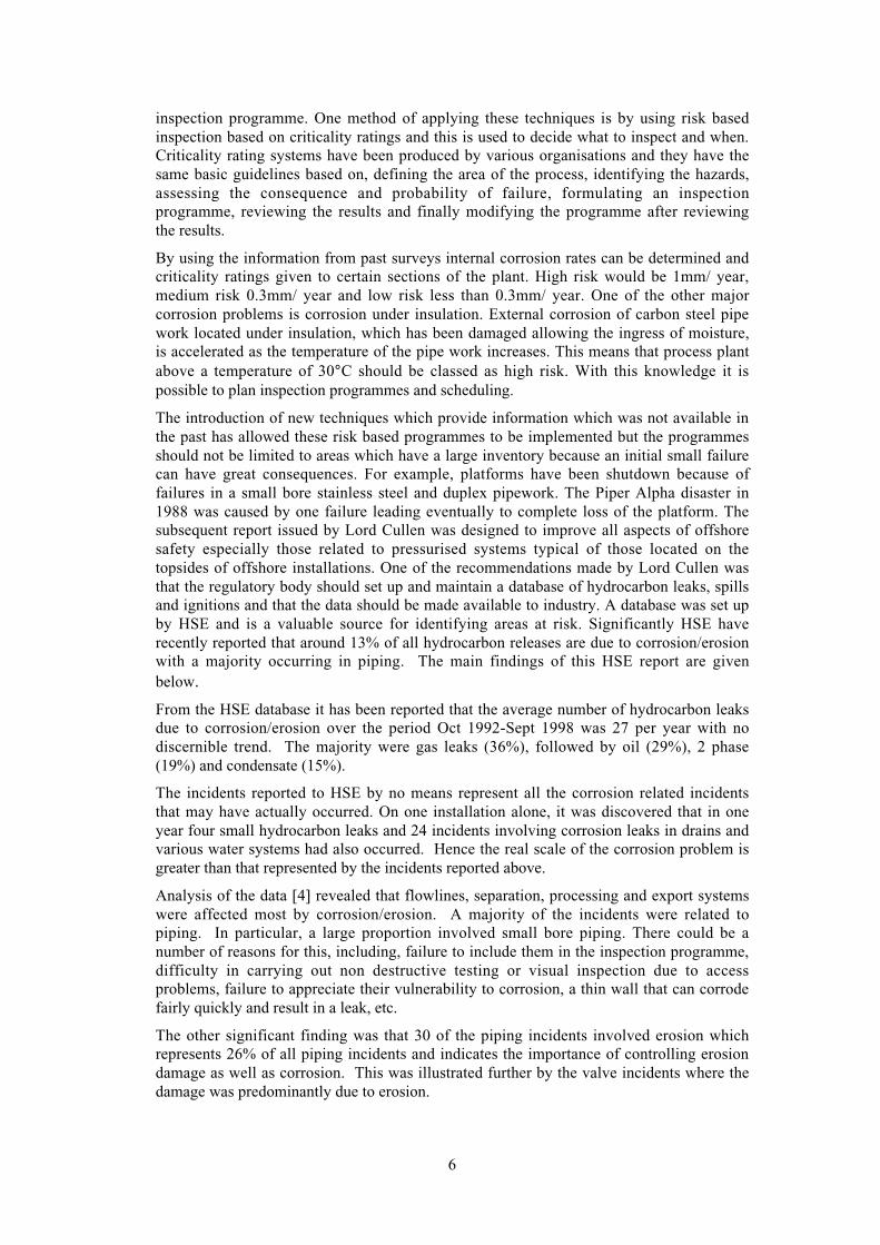
Figure 4 Incotest RACH Trial

Figure 5 LORUS RACH Trial

Figure 6 DMP RACH Trial

13

Figure 7 Micromap RACH Trial

Figure 8 TOFD RACH Trial

Figure 9 Teletest RACH Trial

14

After completion of each trial, BV required the following documentation to be provided. ATrial Report containing details of any changes or revisions to the Test Plan or TestProcedure, and a set of the Trial Results produced by the inspection teams.

15

7. POD RESULTS

Trials were undertaken at TWI under the supervision of BV. The data obtained was interms of defect detection and defect sizing. The sample size was chosen so that in excessof 90 defects were available allowing three groups of 29 defects to be assessed givingthree points on the basic POD curve. From this data the POD at a confidence level of 95%could be determined for the bare pipe trials. For the coated pipe, insulated pipe and bendtrials, a reduced set of defects was used. Tables 2-5 show the main results from the trials.

Table 2 shows the results for the bare pipe trials using A-scan, A-scan with a computerisedpositioning system, magnetic flux leakage and creeping wave.

POD Value(%) for individual defect sizeranges in (mm)

Trial No. Technique 1.3 – 1.8 1.9 – 2.2 2.3 – 2.9 3+

1 A-Scan 33 43 74 90

2 Computerised A-Scan 31 67 100 100

3 Magnetic flux leakage 52 48 35 45

4 Creeping Wave 63 86 84 90

Table 2 POD results for bare pipe

Table 3 shows the results for a second group of trials but this time using coated pipes and areduced sample of defects. The techniques tested included A-scan, A-scan with acomputerised positioning system, and creeping wave. Different defect size ranges werenecessary for Table 3 otherwise the groups would have been too small.

POD Value(%) for individual defectsize ranges in (mm)

Trial No. Technique 1.2 – 2.0 2.1-4.2

5 A-Scan 23 79

6 Computerised A-Scan 85 93

7 Creeping Wave 77 71

Table 3 POD results for coated pipe

Table 4 shows the results for a third group of trials where inspection was attemptedthrough insulation. Only two techniques were used for these trials namely Incotest and thedifferential magnetic probe. Again different groupings have had to be used because of therestricted sample used.

16

POD value (%) for individual defect size(or %wall thickness) ranges

Trial No. Technique 0-34% 35-45% 45%

8 Incotest* 25 40 75

1.4-2.8mm 2.9-4.5mm 4.6+mm

9 Differential MagneticProbe

23 29 56

* Reduced set of defects (only defects consisting of wall thinning over a significant area)

Table 4 POD results for insulated pipe

The final series of trials involved inspection techniques that could be used for relativelylong range inspection. These included LORUS and Teletest and the results are given inTable 5.

POD value (%) for individual defect sizerange (%wall thickness or defect size mm)

Trial No. Technique 0-34% 35-45% 45%

10 LORUS 60 40 60

<3mm >3mm

11 Teletest 25 60

Table 5 Long range inspection data

During the trials it was also possible to measure defect size with some of the inspectionsystems. Figures 10-12 show the results on bare pipe taken during Trials 1,2 & 4. In eachcase the trial data is compared to the characterised data obtained prior to trials. Thus they-axis is the ratio of trial data to characterised wall thickness and the x-axis is the depth ofthe defect as measured in the characterisation work prior to trials.

17

0.0

0.5

1.0

1.5

2.0

2.5

0 2 4 6 8 10

Characterised depth (mm)

Rat

io tr

ial d

ata/

char

acte

rised

dat

a

Figure 10 A-Scan Tested on Bare Steel Cumulated Thickness

0.00

0.50

1.00

1.50

2.00

2.50

0 2 4 6 8 10

Trial data (mm)

Rat

io o

f tria

l / C

hara

cter

ised

dat

a

Figure 11 Micromap Tested on Bare Steel Cumulated Thickness

18

0.00

0.50

1.00

1.50

2.00

2.50

0 2 4 6 8 10

Trial data (mm)

ratio

of t

rial/C

hara

cter

ised

dat

a

Figure 12 CHIME Tested on Bare Steel Cumulated Thickness

Figures 13 & 14 show the results for coated pipes (Trials 5 & 6) and Figure 15 shows theresults for insulated pipe from Trial No. 9.

0.00

0.50

1.00

1.50

2.00

2.50

0 2 4 6 8 10

Trial data (mm)

Rat

io o

f tria

l/Cha

ract

eris

ed d

ata

Figure 13 A-Scan Tested on Coated Steel Cumulated Thickness

19

0.00

0.50

1.00

1.50

2.00

2.50

0 2 4 6 8 10

Trial data (mm)

Rat

io o

f tria

l/Cha

ract

eris

ed d

ata

Figure 14 Computerised A-Scan Tested on Coated Steel Cumulated Thickness

0.00

0.50

1.00

1.50

2.00

2.50

0 2 4 6 8 10

Trial data (mm)

Rat

io o

f tria

l/Cha

ract

eris

ed d

ata

Figure 15 DMP Tested on insulated Steel Cumulated Thickness

Finally a record was kept of any spurious indications for each technique. This informationwas used to produce reliability operating characteristic plots. Figure 16 shows the resultsfor Trials 1-4 and 11, on bare pipes, and Figure 17 shows the results from coated pipes(Trials 5 & 6). Figure 17 also has the result from Trial No. 9 on insulated pipes.

20

0

20

40

60

80

100

0 20 40 60 80 100

Spurious (%)

Pro

babi

lity

of D

etec

tion

(%) A-Scan

ComputerisedAScanMFL

Creeping Wave

Teletest

Figure 16 Reliability Operating Characteristic(ROC) for bare Steel Cumulated Thickness

0

20

40

60

80

100

0 20 40 60 80 100

Spurious (%)

Pro

babi

lity

of D

etec

tion

(%)

A-Scan coated

Computerised A-Scan coated

DMP insulatedpipe

Figure 17 Reliability Operating Characteristic

21

8. CORROSION RELIABILITY ANALYSIS

Reliability analysis is required in situations where values of quantities used in calculationsare not known accurately. Instead of a simple value, a central tendency and spread are usedto describe these quantities.

In corrosion it is necessary to consider two variables, load and strength and estimate bothin probabilistic terms. Figure 18 shows a typical case where the strength exceeds the loadin most circumstances but there is an overlap, the shaded area, and this possible failureregion is regarded as the probability of failure (POF).

The expression (strength – load) >0 represents the situation where a component orstructure is safe and is called the limit state function. These functions can be expressed interms of defect size.

A BµL µS

Probability

Load Strength

Load/Strength units

Figure 18 Basic Structural Reliability

In practice the POF will almost always be a small value (e.g. <10-3) and this needs to becalculated for a structure or component in terms of how it varies due to degradation inservice. Often a related parameter, the reliability index β, is calculated for convenience.The method of derivation is explained below.

The reliability graph shown in Figure 18 can be redrawn as a graph of load againststrength, as shown in Figure 19.

22

Load

StrengthµS

1

2

3

4

A

1 2 3 4 5

µL

B

Load = Strength

c

Failure Region

⟨

Figure 19 Load versus strength reliability diagram

Anywhere that the load is greater than strength (i.e. to the left of the load = strength line)is the failure region. In the particular case of Figure 19 this is represented by the smalltriangle shown (ignoring the tails of the distributions, for simplicity). Again, it can be seenthat decreasing strength or increasing spread increases the area of the triangle and the POF.

If the origin of this graph is set at the central tendency values of load and strength, the load= strength line is displaced, as shown in Figure 20.

34

2

1

321 5

4

5

Strength

Load = Strength Load

A

B

Figure 20 Reliability diagram with axes displaced to central tendency values

23

The effect of inspection is to provide a new estimate of the reliability based on a re-calculated structural strength. The sensitivity and accuracy of the techniques affect thereliability calculations.

The reliability is said to be updated by the inspection process. The updating can be a staticcase (i.e. simply recalculated at the new inspection time) or may include degradationmodels. The latter are needed to produce inspection schedules. Use of knowledge of thedegradation process also allows the possibility of Bayesian updating. This uses apreliminary predicted value of the reliability based on the degradation model from initialconditions or from the last inspection, and performs a different calculation to produce theupdated reliability.

The distance of the load = strength line from the origin can be calculated. Clearly thisdistance will decrease as the strength reduces; beta will also become smaller.

The procedure for calculating the reliability index, β, for a component subjected tocorrosion can be illustrated as follows. In this example the probability distributions for thestrength, and load are given and assumed to be normal. The example particularlyillustrates how time dependent degradation processes such as corrosion can beimplemented in the estimation of the reliability index for a give set of defined variables.

For the standard case involving two distributions of load (L) and strength (S) and where Land S are uncorrelated, the reliability index, β, can be calculated from;

( )22LS

LS

σσ

µµβ+

−= (1)

where Sµ and Lµ are the mean strength and mean load respectively while Sσ and Lσare the standard deviations for the strength and load respectively. This definition of β isinvariant to the definition of the failure function and it is only applicable where the failuresurface depends only on two standard variables S and L. In practice, often the failuresurface depends on more than just two variables but these are often correlated, and thecorrelation coefficients must be used in determining the reliability index. Where severalvariables are involved it is still possible to linearise the safety margin provided that thecorrelation between any pair of basic variables are accounted for by using the appropriatecorrelation coefficients.

The example of this procedure is based on a pipe subjected to corrosion. It assumes thatthe distribution of strength per unit cross sectional area, s, for a pipe is normallydistributed ( )6 ,20 == ssN σµ . In this case it is assumed that A is also normally

distributed, ( )44.0 ,1 == AAN σµ . These two standard uncorrelated variables can beused to determine the overall distribution of strength, S, which will also be normallydistributed with the following parameters.

( ) ??

==

==

64.2

20

22sASA

sASA

σσσ

µµµ(2)

This overall distribution of strength is shown in Figure 21, where it is compared with anormally distributed load ( )2 ,10 == LLN σµ .

24

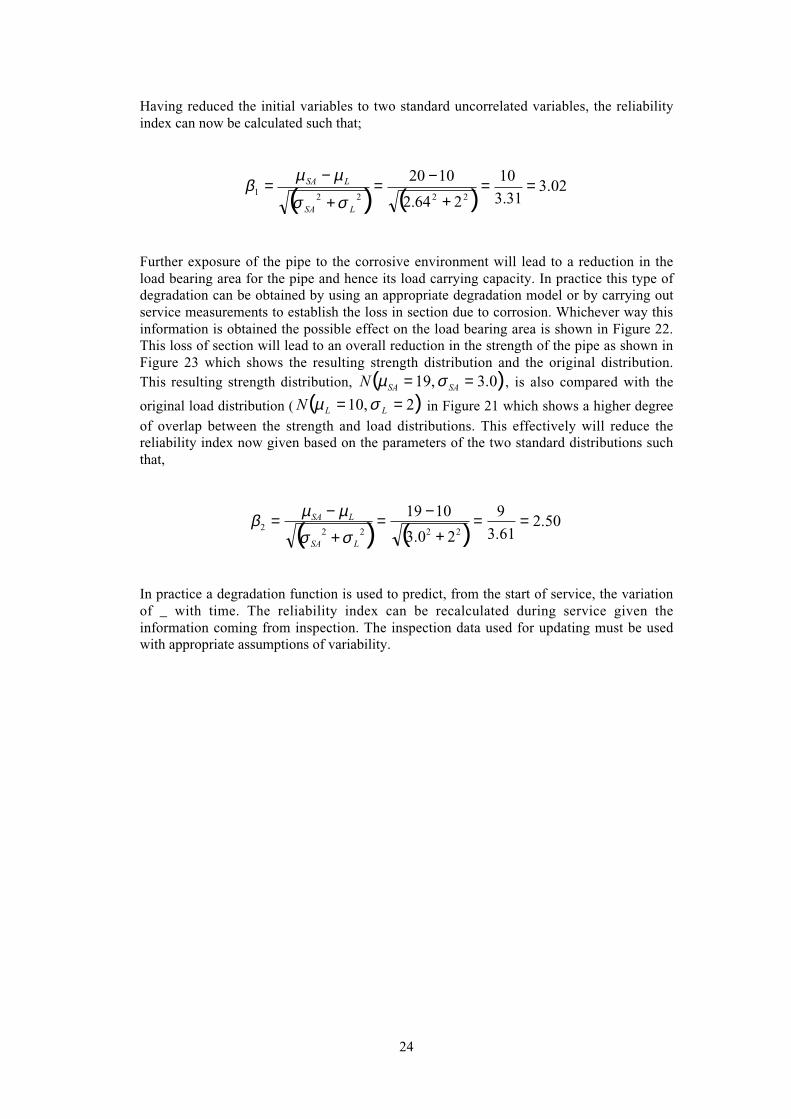
Having reduced the initial variables to two standard uncorrelated variables, the reliabilityindex can now be calculated such that;

( ) ( ) 02.331.3

10

264.2

102022221 ==

+

−=+

−=

LSA

LSA

σσ

µµβ

Further exposure of the pipe to the corrosive environment will lead to a reduction in theload bearing area for the pipe and hence its load carrying capacity. In practice this type ofdegradation can be obtained by using an appropriate degradation model or by carrying outservice measurements to establish the loss in section due to corrosion. Whichever way thisinformation is obtained the possible effect on the load bearing area is shown in Figure 22.This loss of section will lead to an overall reduction in the strength of the pipe as shown inFigure 23 which shows the resulting strength distribution and the original distribution.This resulting strength distribution, ( )0.3 ,19 == SASAN σµ , is also compared with the

original load distribution ( ( )2 ,10 == LLN σµ in Figure 21 which shows a higher degreeof overlap between the strength and load distributions. This effectively will reduce thereliability index now given based on the parameters of the two standard distributions suchthat,

( ) ( ) 50.261.3

9

20.3

101922222 ==

+−=

+

−=LSA

LSA

σσ

µµβ

In practice a degradation function is used to predict, from the start of service, the variationof _ with time. The reliability index can be recalculated during service given theinformation coming from inspection. The inspection data used for updating must be usedwith appropriate assumptions of variability.

25

Original Load and strength distribution

0

0.05

0.1

0.15

0.2

0.25

0.3

0.00 5.00 10.00 15.00 20.00 25.00 30.00 35.00 40.00 45.00 50.00

Load

Pro

bab

ility

Load (L), Original

SA, Original

Figure 21 Distribution of standard variables used in calculating 1β

Distribution of load bearing area

0

0.1

0.2

0.3

0.4

0.5

0.6

0.7

0.8

0.9

1

0.000000 1.000000 2.000000 3.000000 4.000000 5.000000 6.000000

Area Units^2

Pro

bab

ility

Area (A), New

Area (A), Original

Figure 22 Effect of degradation on the distribution of load bearing area for 2β

26

Distribution of strength

0

0.05

0.1

0.15

0.2

0.25

0.3

0.00 5.00 10.00 15.00 20.00 25.00 30.00 35.00 40.00 45.00 50.00

Strength

Pro

bab

ility

SA, New

SA, Original

Figure 23 Effect of degradation of distribution of strength for 2β

Software such as Strurel or Comrel [5] is available for the calculation of β and in RACH[6], Comrel was used in conjunction with limit state functions derived from varioussources (ANSI B 31G [6], RSTRENG) and a corrosion pit growth model.

The aim of the analysis is to quantify the time dependent failure probability. This requiresthe use of the time variant form of COMREL (COMREL –TV). This is more complexthan the time invariant analysis as it requires the consideration of random processes whichare not necessarily stationary with respect to time.

The most important aspects for reliability based inspection scheduling are as follows:

To give assurance of integrity for a given service period (a degradation model is requiredfor this).

Updating of computed reliability using inspection data.

The defect growth model incorporated into RACH is of the form shown in equation (1).

Depth of pit (d) = K t n (1)

Where t is time and K and n are constants depending on the environment, material etc.This is used in conjunction with either of several limit state functions taken from codes(ANSI B 31G, RSTRENG, or API 579 Level 2 and 3).

For integrity assurance one has to adopt a target reliability level. In addition a predictedreliability curve estimated in terms of service life needs to be produced. This then allowsthe choice of inspection interval.

27

The purpose of reliability updating is to reduce the knowledge uncertainty by taking intoaccount the most recent observations (inspection data). This needs to include theuncertainty associated with inspection sizing accuracy.

Two problems exist in terms of the inspection data. One is the accuracy of sizing and theother is the likelihood of detection. The second point also has two aspects ie whether theinspection is in control or whether the detection level is poor. Probability of Detection datawill be relevant to the last of these two but knowledge of the degradation mechanism isnecessary to show which inspection equipment should be used.

The difficulty associated with implementing inspection data into reliability updating, andthe advantages of using more accurate measurements, can be visualised from the followingexample based on three types of inspection data.

Type A produces thickness measurements directly, with a resolution that is expected to begood (1% is shown), and is the type of data expected from ultrasonic thickness gauging.Figure 24 shows an example of a set of readings for one particular application. This typeof data is very dependent on the sampling approach used to collect data. Given full(100%) sampling a distribution like Figure 24 is possible.

0

10

20

30

40

50

60

70

80

90

100

0 5 10 15 20 25

Thickness Loss(% wall)

No

of

Rea

din

gs

Figure 24 Example of high resolution wall thickness readings

Type B is a system that has a known POD of 1-exp(-0.1221x) (where x is the wallthickness loss). This relationship shows, for example, that the equipment has a POD ofapproximately 95% at 25% wall loss. Some flux leakage devices, ACFM, the radiographysystem and the low frequency ultrasonics may have data in a format that can be interpretedin this way.

Type C is a system that separates its received data into 20% wall loss intervals. Due to thelow resolution of Type C 20% of the data recorded as being in the 0-20% range is actually20-40%. In addition 20 % of the data recorded as being in the 20-40% range is actually 0-20% and 20% is 40-60%. Some flux leakage systems produce output in this format.

28

In order to compare the use of these three different types of inspection data an example ofin-service degradation needs to be considered. Figure 25 shows a statistical representationof the result of a particular deterioration mechanism. The graphs show the expectedthickness after periods of 5 years. In practice other deterioration mechanisms will givedifferent forms of this graph. The form may be known from previous plant experience butmay be less well known in new plant or plant where conditions have or will change.

-0.02

0

0.02

0.04

0.06

0.08

0.1

0.12

0.14

0.16

0 20 40 60 80 100

Defect Size

Pro

bab

ility

Den

sity

Year 5Year 10Year 15Year 20

Figure 25 Example of Deterioration Mechanism

As mentioned earlier the limit function can be expressed in terms of defect size. Thus theextra shaded area under the tail of the distribution in Figure 26 can represent theprobability of failure.

29

0

0.05

0.1

0.15

0.2

0.25

0.3

0.35

1 12 23 34 45 56 67 78 89 100 111 122 133 144 155 166 177 188 199

Defect Size

Pro

bab

ility

Wall Thickness/Withdrawal Criteria

Probability of Failure

Figure 26 Probability Density of Defect Size showing Probability of Failure

Combining Figures 25 and 26 can give something like Figure 27, which shows how thePOF varies with time. A point on this curve may be chosen as the target reliability figureat which it may be necessary to take action (for example probability of failure 10-3).

1.00E-08

1.00E-07

1.00E-06

1.00E-05

1.00E-04

1.00E-03

1.00E-02

1.00E-01

1.00E+000 5 10 15 20

Time

PO

F

Figure 27 Change of POF with Time

30

To compare the three types of data the following results are assumed for an inspection atYear 10.

a) Equipment A results are as given in Figure 24.

b) Equipment B results gave no indications of defects.

c) Equipment C results gave 80% of data points in the range 0-20% wall thickness loss and20% data points in the range for 20-40% wall thickness loss.

Firstly, for equipment A, Figure 25 showing, the expected thickness distribution, can becompared with the measured defect distribution given in Figure 24. It can be seen that themeasured distribution agrees closely with the defect distribution after 5 years and theprobability of failure estimated after this inspection (from Figure 27) would be 2x10-8.

To analyse an inspection carried out by Equipment B with no defects detected, it isnecessary to consider the probability of a defect being present together with the POD. Thismay be represented by the diagram in Figure 28. For any particular defect size range, andat any particular time, the probability that there is a defect is given by Area A, and thePOD by Area B. Area A will correspond to the probabilities for individual size rangeswithin the graphs in Figure 25, and Area B will be 0 at zero defect size and increase as thedefect size increases.

Figure 28 Probabilities for an Inspection at a particular time

A- Probability of defect of certain size being present

B- Probability of Detection for that size

Overlap Area-Probability of a defect being present and detected by the inspection

The overlap of the two is the probability that a defect will be present and detected. Thetotal probability over all sizes can be calculated by summing the values for all size ranges.The probability that a defect will be detected using Equipment B at any inspection time,and therefore the probability that an inspection could be carried out with no defects at eachinspection time can be calculated.

If no defects are detected, a choice of an appropriate probability must be made to estimatethe year to which the deterioration has progressed. Suppose that a 10% probability isconsidered acceptable, then, on the basis of the calculations described above, this would

31

give a defect distribution in Year 8 (say) and a POF of 5x10-6. A consideration ofconfidence intervals in this data is likely to be most important in this type of analysis.

The situation for equipment C is rather more complex. Suppose an inspection result gives80% in the range 0-20% wall loss and 20% of results in the range 20-40% loss. Using acorrection for the errors as mentioned earlier, a final estimated defect distribution can becalculated.

If the defect distribution curves in Figure 25 are replotted in 20% ranges, the results of theinspection can be compared directly with the defect distribution for equipment C, as inFigure 29. It can be seen that in this case a reasonable correspondence is with thedistribution in year 10 (giving a POF of 3 x 10-5 ).

0102030405060708090

100

0-20 20-40 40-60 60-80 80-100

Wall Thickness Loss(%)

% o

f D

efec

ts Inspection Results

Year 10 DefectDistribution

Figure 29 Comparison of Inspection Results and Year10 Distribution

The above data gives some idea of how to estimate the current POF from an inspectionresult with known inspection reliability data. In order to assess the date of the nextinspection the target POF needs to be known together with an existing timescale.

If one takes the target POF to be 10-3, and all the inspections above had been carried out inYear 10 then examination of Figure 30 shows that in the case of the inspection carried outby the high resolution device the deterioration mechanism appears to have not taken placeas fast as expected, and the expected progression indicates a life of 8 years beforewithdrawal. Inspection B shows that the target POF will be in Year 15, and Inspection Creaches the target POF in Year 13.

32

1.00E-11

1.00E-10

1.00E-09

1.00E-08

1.00E-07

1.00E-06

1.00E-05

1.00E-04

1.00E-03

1.00E-02

1.00E-01

1.00E+000 5 10 15 20 25

Time(years)

PO

F

POF originally expected

POF given results ofInspection A

POF given results ofInspection B

POF given results ofInspection CTarget POF for withdrawal

=

Figure 30 Effect of Inspections on POF and Lifetimes

33

9. ANALYSIS OF SERVICE DATA

The final example looks at service data and illustrates lack of control in inspection. InRACH a procedure for manual updating for inspection scheduling for corrosion defectswas developed. This was used for assessing a service case history. The steps are asfollows:

Establish the ‘a priori’ curve for β as a function of time.

Choose a minimum target reliability level (β) and hence decide on the date for inspection.

Specify an inspection method which is able to detect a defect size equal to the onepredicted.

Update the predicted defect size by using the inspection outcome and continue theprediction from that point to give an ‘a posteriori’ curve.

The service example is based on a mature system installed in 1983 in the North Sea for a20 year life. The topside pipework was inspected frequently with A-scan and occasionallywith A-scan incorporating a computerised positioning system. Thus two sorts of inspectiondata are available for analysis representing two inspection strategies. Both strategies arebased on UT data but one with a specified grid along the pipe (referred to as UT) the othera detailed measurement of wall thickness for the whole pipe (referred to as µMap)

Annual data using these two approaches is shown in Table 6. Examples of individual setsof data are shown in Figures 31 and 32.

Line Number Date Inspected Nominal WTMinimum Reading

RecordedTechnique

1 09/03/1995 9.27 7.2 UT

30/06/1996 9.27 6 UT

15/04/1997 9.27 5.79 Map

28/08/1998 9.27 5.25 UT

31/08/1997 9.27 4.75 UT

25/10/1998 9.27 2 Map

2 21/09/1991 7.78 9 UT

30/06/1996 7.78 8.99 UT

15/04/1997 7.78 1.79 Map

28/08/1997 7.78 7.75 UT

Table 6 In-Service inspection data

34

Wall Thickness for Line 1

0

1

2

3

4

5

6

7

8

94 95 96 97 98 99

Inspection Date

Thic

knes

s (m

m)

UT

Umap

Log. (UT)

Figure 31 Historical Inspection Data

Wall Thickness for Line 2

0

2

4

6

8

10

90 92 94 96 98

Inspection Date

Thic

knes

s (m

m)

UT

Umap

Log. (UT)

Figure 32 Historical Inspection Data

The historical data can be seen to be very dependent on the inspection strategy. Figures 31& 32 appear to show two types of behaviour, widespread corrosion or localised corrosion.Line 1 for example appears to give similar results for UT and µMap. Thus even without100% coverage significant wall loss was detected. The corrosion in the pipe must havebeen widespread.

A check on the distribution measured by µMap, seen in Figure 33, confirms this as manydefects were detected and the average remaining wall thickness was between 5 and 6mm.

35

This represents nearly 50% wall loss for the average measurement. Thus even UT wasmeasuring significant corrosion.

Line 2 Micromap data for 1997

0

10

20

30

40

50

1 3 5 7 9 11 13 15 17

Thickness range

No

of

occ

urr

ence

s

Figure 33 Line distribution of measured wall thickness

In contrast Line 2, Figure 32, shows wide differences between UT and µMap. In thesecases the UT inspection was not sufficiently in control and was not detecting thesignificant flaws. The detailed MicroMap data for 1997 showed that the distribution wasvery different to that shown in Figure 33 and that only a few were around 2 mm and thenormal distribution was centred around 10mm. Thus with only a few measurements thesignificant defects may be missed.

The analysis can be expressed in a different way using the software developed with RACHfor a probabilistic assessment. This can be done in association with the trials dataproduced for the µMap technique.

The trials data showed that wall thickness loss in excess of say 2.5 mm could be detectedwith a very high POD at a high confidence level. In addition the accuracy of wall lossprediction approached a very high accuracy at about 3 mm loss. Thus periodic use ofµMap on line with a corrosion allowance of 3.2 mm (as in the present case) would ensuredetection before failure.

A-scan trials data showed that a wall thickness loss nearer to 4 mm is needed beforereaching a very high POD and that in combination with a persistent underestimate of 20%the periodic use of this technique would not guarantee detection within the corrosiveallowance of 3.2 mm.

Given appropriate choices for the degradation model it is also possible to produce therelevant β values necessary for inspection scheduling. Figure 34 shows this schedulingdata for Line 2, produced using the RACH software.

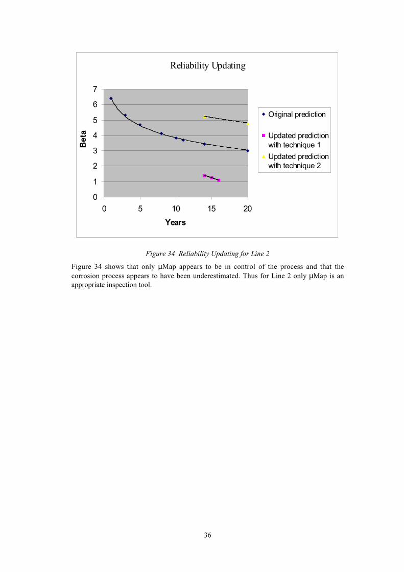
36

Reliability Updating

0

1

2

3

4

5

6

7

0 5 10 15 20

Years

Bet

a

Original prediction

Updated predictionwith technique 1

Updated predictionwith technique 2

Figure 34 Reliability Updating for Line 2

Figure 34 shows that only µMap appears to be in control of the process and that thecorrosion process appears to have been underestimated. Thus for Line 2 only µMap is anappropriate inspection tool.

37

10. SUMMARY AND CONCLUSIONS

10.1. SUMMARY

The initial reviews and the information received from the Health and Safety Executive,Shell and Marathon showed that the project needed to address the problem of corrosionand erosion in pipework. This is still a cause for concern and can give problems includingthe release of hydrocarbons.

Corrosion modelling identified three types of corrosion (general, local metal loss, andpitting corrosion) and produced typical growth rate equations. These together with thelimit state functions were coded into the COMREL reliability program to give corrosionreliability inspection scheduling. The version used in this work was the Time Variant sothat updating from in-service data was possible. In essence this program produces thevalue of β for a particular situation (where β is related to the failure probability and forscheduling is a more convenient program output).

β values are produced in a particular case for specific intervals in a service life, and, givena target value of β for safety purposes, an inspection schedule is constructed. Theunknown or unforeseen possibilities of damage in service are taken into account by thecalculated values of β based on in-service data. Thus an updated β curve can be comparedto the original β curve and amendments made to the inspection schedule based on acomparison of these curves.

Demonstration trials involved, inspection reliability trials, laboratory trials and field trials.The preliminary survey of POD data revealed that there was nothing suitable for thedetection of isolated local metal loss or pitting and, given the importance of this data forprobabilistic based inspection scheduling, POD trials were necessary.

The trials were conducted under the supervision of BV, in order to give manufacturersassurance of impartiality, at the facilities of TWI using the sample produced at UCL. Strictcontrol of data and interpretation was enforced by BV and the results are given onsignificant first step in the provision of quantitative data on inspection reliability forcorrosion.

The results showed that 100% inspection with UT could, in the best circumstances, giveexcellent results in terms of defect detection and sizing. Other results also showed thatsome of the newer techniques although promising in terms of economic use still requiredfurther development before they could achieve the benefits of low cost and high qualitydata.

Laboratory trials and field trials were based on the data produced in the project especiallythe information on corrosion modelling and corrosion reliability inspection scheduling.For the laboratory trials advantage was taken of the corrosion pit production for the PODsample. Attempting various inspection schedules was possible in this laboratory basedwork and could be verified given the access to real defect growth rates. Two particularinspection systems were utilised and compared using the predicted values. The basicdifference between the inspection systems was that in one case the scanning pattern forthickness measurement was quite broad giving the possibility of missing or undersizingsome corrosion pits. The results showed that for the broad scanning pattern the β valueswere insensitive to the defect population and were invariably low in value, something akinto loss of control of the process. The ideal scanning pattern of the other system gave good

38

results and a consistent updating behaviour. The results also showed that both of the limitstate functions coded gave relatively similar predictions.

The field trials were based on a Marathon platform and produced an interesting variety ofsituations. The most frequent situation was of single mode behaviour in that normalsampling showed how the defect population varied with time in service. However bimodalbehaviour also existed and caused problems for the operator. It was necessary in thesecircumstances to have two inspection systems, conventional thickness mapping and µ Mapa more intense and elaborate survey. µ Map located and sized defects in both populations,general corrosion and local metal loss / pitting. It was clear from this work that anyoccasional periodic check with µ Map linked to more regular conventional wall –thicknesssurveys could give control of the degradation process.

10.2. CONCLUSIONS

The RACH project has provided data and analysis methodology suited for rationalinspection scheduling. The defect sample and POD trials results together with defectgrowth rate models and limit state functions used in conjunction with COMREL –TV, hasallowed the development of corrosion reliability analysis.

The results show that thickness measurement can be very accurate but that samplingpattern have a strong influence on the detection of corrosion.

All of the information on NDT equipment and procedures is stored on the RACH databasetogether with the inspection reliability results [8].

a) Corrosion and erosion are still a problem in offshore process plant even in plainpipes.

b) A wide range of NDT equipment is now available for detection of wall loss andwith 100% inspection and removal of cladding very good results can be obtained.In more difficult situations such as inspection through thick coating improvementin NDT equipment is still needed.

c) Probability based inspection scheduling is now possible but requires informationon the defect distribution and the change in distribution during service life. Inservice measurements are necessary to provide the input but this needs to be donethrough consideration of the probability of detection.

d) Eight techniques were subjected to rigorous trials to give POD and sizing accuracydata. Of these the 100% thickness measurement UT systems used on bare metalwere very successful. It was not possible to include X-ray techniques and thiswork is still necessary.

e) Corrosion modelling was studied and reviewed and typical growth rates and limitstate functions were coded for corrosion reliability inspection scheduling. Fieldtrials showed that the software based on COMREL-TV could be applied to servicedata in principal but that the nature of corrosion could be quite complex leading toa combined distribution of defects. Further modelling and validation work isrequired before the probability based corrosion reliability inspection can beconfidently used.

39

11. ACKNOWLEDGEMENTS

The RACH Partners would like to acknowledgement the financial support of the EUDGXVII (THERMIE Programme), Shell UK Exploration and Production, Marathon OilUK Limited and the Health and Safety Executive.

12. REFERENCES

1) Reliability Assessment for Containers of Hazardous Materials Contract NumberOG/112/95/Fr-UK Thermie DGXVII.

2) DRAFT Document prepared by the UKOOA Inspection Engineering Work Group“Guidelines for the use of Criticality Assessment to Establish InspectionRequirements for Pressure Systems on UK Offshore Oil & Gas Installations. 18October 1991.

3) Still, J.R., Nelson, P., Development of Corrosion Monitoring in the Offshoreproduction Industry. British Journal of NDT Vol. 34 No. 7 July 1992.

4) Patel, R., Rudlin, J., Analysis of Corrosion/Erosion Incidents in Offshore ProcessPlant and Implications for Non-destructive Testing. Insight Vol.42 No.1 January 2000.

5) Strurel - RCP. Reliability Consulting Programs, Barerstr. 48, D-80799 Munich,Germany.

6) RACH Report on Reliability Studies 99/302/00.

7) ASME B31G (1991): Manual for determining the remaining strength of corrodedpipelines.

8) RACH Final Report, September 1999 Available from TSC Inspection Systems, 6 MillSquare, Featherstone Road, Wolverton Mill, Milton Keynes MK12 5RB, UK.

Printed and published by the Health and Safety ExecutiveC0.35 4/01

OTO 2000/095

£20.00 9 780717 620142

ISBN 0-7176-2014-X