offshore vertical axis wind turbine with floating and...
TRANSCRIPT

General rights Copyright and moral rights for the publications made accessible in the public portal are retained by the authors and/or other copyright owners and it is a condition of accessing publications that users recognise and abide by the legal requirements associated with these rights.
• Users may download and print one copy of any publication from the public portal for the purpose of private study or research. • You may not further distribute the material or use it for any profit-making activity or commercial gain • You may freely distribute the URL identifying the publication in the public portal
If you believe that this document breaches copyright please contact us providing details, and we will remove access to the work immediately and investigate your claim.
Downloaded from orbit.dtu.dk on: Jun 04, 2018
Offshore Vertical Axis Wind Turbine with Floating and Rotating Foundation
Vita, Luca; Friis Pedersen, Troels; Aagaard Madsen , Helge
Publication date:2011
Document VersionPublisher's PDF, also known as Version of record
Link back to DTU Orbit
Citation (APA):Vita, L., Friis Pedersen, T., & Aagaard Madsen, H. (2011). Offshore Vertical Axis Wind Turbine with Floating andRotating Foundation. Kgs. Lyngby, Denmark: Technical University of Denmark (DTU).

Ris
ø-Ph
D-R
epor
t
Offshore Floating Vertical Axis Wind Turbines with Rotating Platform
Luca Vita Risø-PhD-80(EN) August 2011

Risø-PhD-80(EN)
Author: Vita, LucaTitle: Offshore floating Vertical Axis Wind Turbines with Rotating Platform Division: Wind Energy Division
Risø-PhD-80(EN) August 2011
The fast growth of the wind energy market has increased the strategic importance of offshore wind energy, addressing the need for new offshore wind turbine concepts.
This work deals with a new offshore floating wind turbine concept, using a Vertical Axis Wind Turbine (VAWT) as rotor and a floating rotating platform as foundation. My research investigates the feasibility and the potentials of the concept.
The first step of my research is the study of the loads acting on the floating VAWT. Since the platform is rotating, a water stream generates a hydrodynamic force on the structure, known as Magnus effect. Also a friction moment acts on the platform. A CFD investigation is carried out to find out the non dimensional force coefficients at different rotational speeds of the platform.
The second step is to adapt a numerical solver, to carry out a numerical simulation of the concept. I used the software HAWC2 from Risø DTU and I added some DLLs to make it capable of investigating a floating VAWT.
I design the new concept for three different sizes:
- A 2MW size, mostly used during the code adaptation process to evaluate the code.
- A 5MW size, which I selected as the proper size for a baseline model.
- A 1kW size, which I designed as a downscaled model to use for experimental test verifications.
The last step of my investigation is a rough estimation of the economical potentials of the new concept, compared to an offshore floating HAWT concept.
(The thesis is submitted to the Danish Technical University in partial fulfilment of the requirements for the PhD degree)
ISSN 0106-2840 ISBN 978-87-550-3924-7
Contract no.:
Group's own reg. no.: 1125007-01
Sponsorship: Wind Energy Department and DeepWind fp7 European Project Cover : Artistic view of the DeepWind concept.
Pages:164 References:
Information Service Department Risø National Laboratory for Sustainable Energy Technical University of Denmark P.O.Box 49 DK-4000 Roskilde Denmark Telephone +45 46774005 [email protected] Fax +45 46774013 www.risoe.dtu.dk

iii Risø-PhD-80(EN)
Contents CONTENTS ...................................................................................................................... III
ACKNOWLEDGMENTS ..................................................................................................... VI
PREFACE ........................................................................................................................ VII
NOMENCLATURE .......................................................................................................... VIII
1 INTRODUCTION ........................................................................................................ 1
1.1 OBJECTIVES ................................................................................................................ 1
1.2 STATE OF THE ART ........................................................................................................ 1
1.2.1 Background: wind power offshore market ......................................................... 1
1.2.2 Brief history of VAWT and floating wind turbines .............................................. 2
1.2.3 Numerical tools for floating VAWTs ................................................................... 9
1.3 THESIS OUTLINE ......................................................................................................... 10
1.4 DESIGN APPROACH ..................................................................................................... 12
2 DEEPWIND CONCEPT .............................................................................................. 16
2.1 MAIN CONCEPT DESCRIPTION ....................................................................................... 16
2.2 COMPONENTS ........................................................................................................... 16
2.2.1 Rotor ................................................................................................................. 16
2.2.2 Blades ............................................................................................................... 17
2.2.3 Generator ......................................................................................................... 17
2.2.4 Anchoring ......................................................................................................... 18
2.2.5 Safety system.................................................................................................... 18
2.2.6 Control strategy ................................................................................................ 19
2.3 STRATEGIES FOR INSTALLATION AND OPERATION AND MAINTENANCE ................................... 19
2.3.1 Installation ........................................................................................................ 19
2.3.2 Operation and Mantenaince (0&M) ................................................................. 19
2.4 CONCEPT POTENTIALS ................................................................................................. 20
2.5 SPECIFIC CHALLENGES ................................................................................................. 20
2.6 METHODOLOGY FOR THE INVESTIGATION OF THE CONCEPT AND AVAILABLE CONFIGURATIONS ... 21
2.6.1 First Configuration (Sea bed configuration) ..................................................... 21
2.6.2 Second Configuration (Torque arm fixed configuration) .................................. 22
2.6.3 Third Configuration (Mooring fixed configuration) .......................................... 22
2.7 PROGRESS BEYOND THE VAWT STATE OF THE ART ........................................................... 22
3 LOADS AND DYNAMICS OF A FLOATING VERTICAL AXIS WIND TURBINE .................. 24
3.1 FORMULATION OF THE PROBLEM .................................................................................. 24
3.2 AERODYNAMIC LOADS ON A TWO BLADED VAWT ............................................................ 26
3.3 WAVE‐INDUCED LOADS ............................................................................................... 28
3.3.1 Formulation of the problem and assumptions ................................................. 28
3.3.2 Regular waves and statistical description ........................................................ 28
3.3.3 Hydrostatic loads .............................................................................................. 30
3.3.4 Radiation loads ................................................................................................. 31
3.3.5 Diffraction loads ............................................................................................... 31
3.3.6 Morison’s formulation and the viscous loads and damping ............................. 32

iv Risø-PhD-80(EN)
3.4 EQUATION OF MOTION AND NATURAL PERIODS ................................................................ 33
4 LOADS FROM A WATER STREAM PASSING THE ROTATING PLATFORM .................... 35
4.1 LOADS ON A ROTATING CYLINDER IN A WATER STREAM, PREVIOUS STUDIES ............................ 35
4.2 METHODOLOGY OF THE STUDY ..................................................................................... 37
4.3 RESULTS................................................................................................................... 38
4.4 DISCUSSION .............................................................................................................. 40
4.5 CONCLUSIONS AND SUGGESTIONS FOR FURTHER INVESTIGATIONS ........................................ 42
5 CONCEPT SCALING .................................................................................................. 44
5.1 POSSIBLE METHODOLOGIES .......................................................................................... 44
5.2 PHYSICAL SCALING OF THE PHENOMENA: MODEL SCALING .................................................. 44
5.3 FEASIBILITY APPROACH: CONCEPT SCALING ...................................................................... 46
5.4 ECONOMICAL AND PRODUCTION APPROACH: EVALUATION OF CONCEPT UPSCALING ................ 47
6 NUMERICAL CODE TO INVESTIGATE THE CONCEPT .................................................. 48
6.1 HAWC2 .................................................................................................................. 48
6.1.1 Structural formulation ...................................................................................... 48
6.1.2 Hydrodynamic module ..................................................................................... 48
6.2 ADDED DLLS ............................................................................................................ 49
6.2.1 VAWT aerodynamics ........................................................................................ 49
6.3 FORCES ON THE ROTATING PLATFORM ............................................................................ 51
6.3.1 Generator module ............................................................................................ 53
6.3.2 Generator control ............................................................................................. 53
6.4 FIXED SETUP ............................................................................................................. 53
6.4.1 Physical properties ........................................................................................... 53
6.4.2 Description of external conditions .................................................................... 54
6.4.3 Model set up ..................................................................................................... 55
6.4.4 Reference systems ............................................................................................ 55
6.5 CALCULATION POINTS ................................................................................................. 57
6.6 OTHER SOFTWARE USED FOR NUMERICAL SIMULATIONS .................................................... 57
7 FIRST DESIGN: 2MW ............................................................................................... 58
7.1 DESIGN SPECIFICATIONS .............................................................................................. 58
7.1.1 Rotor design ..................................................................................................... 58
7.2 LOAD CASES AND CODE SET UP ...................................................................................... 60
7.2.1 Wind speed ....................................................................................................... 60
7.2.2 Currents ............................................................................................................ 60
7.2.3 Waves ............................................................................................................... 61
7.3 RESULTS................................................................................................................... 61
7.3.1 Load case 0 ....................................................................................................... 62
7.3.2 Load case 1 ....................................................................................................... 63
7.3.3 Load case 2 ....................................................................................................... 65
7.3.4 Load case 3 ....................................................................................................... 67
7.4 DISCUSSION .............................................................................................................. 68
8 BASELINE MODEL: 5MW ......................................................................................... 70
8.1 DESIGN SPECIFICATIONS .............................................................................................. 70
8.1.1 Site description ................................................................................................. 70

v Risø-PhD-80(EN)
8.1.2 Rotor design ..................................................................................................... 72
8.1.3 Platform design ................................................................................................ 76
8.2 SIMULATIONS ............................................................................................................ 79
8.2.1 Load cases description ...................................................................................... 79
8.2.2 Results .............................................................................................................. 79
8.3 DISCUSSIONS OF THE RESULTS ...................................................................................... 85
9 DOWNSCALED MODEL: 1KW ................................................................................... 87
9.1 DESIGN .................................................................................................................... 87
9.1.1 Site description ................................................................................................. 87
9.1.2 Downscaling considerations ............................................................................. 88
9.1.3 Rotor design ..................................................................................................... 89
9.1.4 Platform design ................................................................................................ 91
9.2 RESULTS FROM NUMERICAL SIMULATIONS....................................................................... 95
9.2.1 Natural frequencies of the rotor ....................................................................... 96
9.2.2 On land configurations ..................................................................................... 98
9.2.3 Discussion on the results of the on land configuration ................................... 100
9.2.4 Offshore simulations ...................................................................................... 101
9.2.5 Discussion on results and recommendations on the platform design ............ 105
9.3 CONCLUSIONS ......................................................................................................... 106
10 COST MODELS FOR OFFSHORE FLOATING WIND TURBINES ................................... 108
10.1 COST ANALYSIS OF WIND ENERGY ................................................................................ 108
10.2 DEEPWIND EVALUATION ........................................................................................... 110
11 CONCLUSIONS ...................................................................................................... 117
BIBLIOGRAPHY ............................................................................................................. 121
APPENDIX A ‐ STRUCTURAL INPUT FOR THE NUMERICAL CALCULATIONS ...................... 130
5MW ................................................................................................................................ 130
Tower ........................................................................................................................... 130
Blades .......................................................................................................................... 131
1KW .................................................................................................................................. 133
Tower ........................................................................................................................... 133
Blades .......................................................................................................................... 134
APPENDIX B – ATTACHED PAPERS ................................................................................. 136
A NOVEL FLOATING OFFSHORE WIND TURBINE CONCEPT............................................................. 136
A NOVEL CONCEPT FOR FLOATING OFFSHORE WIND TURBINES: RECENT DEVELOPMENTS IN THE CONCEPT
AND INVESIGATION ON FLUID INTERACTION WITH THE ROTATING FOUNDATION ................................. 148

vi Risø-PhD-80(EN)
Acknowledgments My work has been carried out in the Wind Energy Division at Risø DTU, Roskilde, Denmark. The research has been supervised by Professor Troels F. Pedersen, Senior Researcher Uwe S. Paulsen and Professor Helge A. Madesn.
After three years of work, I have a broad list of people to acknowledge.
If a ranking can be made, when it comes to thank a list of people, my first thanks go to Test and Measurements program (TEM) in Wind Energy Division at Risø, which has also been my first Danish “home”. Thank to all of you to show me that outstanding work can be made with fun.
I own also some personal acknowledgment among the research community at Risø.
Special thanks go to Troels F. Pedersen, to be a reference rather than just a supervisor during these years and to Uwe S. Paulsen for always challenging me with new ideas and thoughts. And thanks to both of them for their incredibly enthusiastic way of working and for bringing me jogging under the rain in Norway.
My gratitude goes to Helge for his help in the aerodynamic part of the thesis and to Torben for his help with HAWC2. Thanks also to Frederik Zahle for the help with the CFD calculations in Chapter 4 and to Per H. Nielsen for his valuable help in dimensioning the blades and in explaining me things.
I am grateful to Poul Hummelshøj to give me the possibility of working on this project, even though there was not a project yet.
I own my gratitude to Uwe S. Paulsen, Troels F. Pedersen, Flemming Rasmussen and Helge A. Madsen to share with me their novel concept idea and let me participate in it.
Part of this work is included in the fp7 European granted project DeepWind. Thanks to all the partners in the project, for their help and contributions.
I would like to acknowledge Stefan Crstensen from DHI for the help in evaluating the met-ocean conditions at the sites, Joachim Reuder from Oceanor for the access to the met-ocean data at Sletringen, Norway and Wei He from Statoil for her suggestions and her challenging curiosity.
Thanks to all the people who have spoilt me during my “thesis lethargy”, especially to Damien, Nikolas and Braulio for their discreet moral support. I am very grateful to Gireesh for his help in reviewing the thesis and supporting me during the process.
Last but absolutely not least, thank to my little Italian world, which I always find there, every time I land in Italy. Grazie.
Eventually I own also an answer to a question I got at my very first day at Risø: yes, I really like to work on vertical axis wind turbines.

vii Risø-PhD-80(EN)
Preface
This work deals with a new concept for floating Vertical Axis Wind Turbine (VAWT), started at Risø-DTU in 2007. The concept has been later called DeepWind concept [1], taking name from the EU granted project DeepWind. In the current work, when I mention DeepWind, I refer to the concept.
During 2007-2008 Risø-DTU prepared a series of reports [2] as a result of a consultancy project for StatOil. The reports were meant to respond to Statoil’s interest in new alternative designs for floating wind turbines, with emphasis in the possible use of VAWTs. In the last report [3] the new concept was presented to Statoil, as a possible candidate for a new floating VAWT design. The report included also a plan on the possible steps for a successful exploitation of the concept potential.
In 2008, the present PhD project started, aiming at exploiting the feasibility and potential of the new VAWT floating concept.
The study was meant to find out the most relevant challenges that could influence the feasibility of the concept and its advantages. Some codes (mainly HAWC2 and a BEM code for VAWT) needed some adaptation in order to reach a satisfactory accuracy for a first evaluation of the concept and of its feasibility.
From 2010 the Ph.D. project was financed, as part of the fp7 European project DeepWind (2010-2014).

viii Risø-PhD-80(EN)
Nomenclature
ax, ay, az Components of the acceleration of the fluid particles, according the potential-flow theory
[m/s2]
Aij Terms of the added mass matrix [kg] - [kg m2]
Aij(2d) 2D added mass coefficients [kg] - [kg m2]
Aw Water plane area [m2]
B Buoyancy [kg]
Bij Terms of the damping matrix [kg/s] - [kg m2/s]
c Chord of the blade [m]
Cd 2D drag coefficient of the platform in oscillatory flow and of the airfoils in
aerodynamics. .
[-]
CD Drag coefficient of the platform in oscillatory
flow .
, or drag coefficient in the
Morison’s equation
[-]
Cij Terms of the restoring matrix [kg m/s2] - [kg m2/s2]
Cl 2D lift coefficient of the tower in oscillatory
flow and of the airfoils in aerodynamics.
.
[-]
Cm Mass coefficient in Morison’s equation [-]
CM Inertial coefficient in Morison’s equation [-]
CP Power coefficient of the rotor,
.
[-]
dx,dy,dz Displacements of the water plane section of
the tower [m]
D Diameter of the rotor tower [m]
DOF Degrees of freedom of the floating system [-]
f1p First odd frequency of the rotor, [Hz]

ix Risø-PhD-80(EN)
f2p First even frequency of the rotor, [Hz]
fP Peak frequency of the wave spectrum [Hz]
fw Wave frequency [Hz]
Fd Hydrodynamic drag force for length unit [N/m]
FD Hydrodynamic drag force [N/m]
fs Safety factor, [-]
FD Hydrodynamic drag force on the tower [N]
Fi Exiting force or exiting moment of the
mode i
[N] - [Nm]
Fl Hydrodynamic lateral force per meter [N/m]
FL Hydrodynamic lateral force [N]
Fn Froude number, [-]
g Acceleration of gravity, 9.81 [m/s2]
h Water depth [m]
H Rotor height [m]
Hg Height generator box [m]
H0 Clearance of the rotor, from the mean water
level or from the ground [m]
Hs Significant wave height [m]
H100 Wave height with annual probability of
exceedance of 10-2 [m]
HP Length of platform (draft) [m]
Htot Total length of the tower, Htot= Hg+HP+ H0+H
[m]
Ixx, Iyy, Izz Inertia moment around the x, y and z axis [km m2]
k Wave number, k=w2/g,
for finite water depth is k tanh(hk)=w2/g
[1/m]
KC Keulegan-Karpenter number, 2 [-]

x Risø-PhD-80(EN)
Lr Reference length [m]
M Mass [kg]
Mij Terms of the Mass matrix [kg] - [kg m2]
N Number of blades [-]
pD Dynamic pressure [kg/(ms2)]
P Power output [kW]
Q Torque on the shaft [Nm]
R Maximum radius of the rotor [m]
RP Maximum external radius of the platform [m]
RT Maximum external radius of the rotor tower [m]
Re Reynolds number, Re=LrUr, with Lr and
Ur, characteristic length and reference
velocity at the site
[-]
Sw Swept rotor Area [m2]
Sii 2nd water plane moment of inertia [kg m2/s2]
Tx, Ty
Lateral and longitudinal components of the
aerodynamic force [N]
Tw Wave period [s]
Th Thickness of the tower [m]
Tni Natural periods of the floating structure in
the i DOF [s]
Tp Peak period of the wave spectrum [s]
ux,uy,uz Water particle velocity components in
oscillatory flow according the potential-flow
theory
[m/s]
U Water current speed [m/s]
v0 Free wind speed at the equatorial height of
the rotor [m/s]
xi Risø-PhD-80(EN)
V Displaced volume of water [m3]
zB Vertical position of the centre of buoyancy [m]
zG Vertical position of the centre of gravity [m]
Speed ratio on the tower, rRT/U [-]
w Waves direction respect to wind speed
direction [deg]
c Current direction respect to wind speed
direction
[deg]
Potential function in potential-flow theory [-]
Tilt angle [deg]
0 Tilt angle at the start [deg]
Tip speed ratio, Rr/v0 [-]
w Wavelength, w gTw2/(2),
for finite depth: wtanh(2hw gTw2/(2)
[m]
i Displacements in the i DOF [m] - [deg]
Kinematic viscosity [m2/s]
Free stream air density [kg/m3]
W Free stream water density [kg/m3]
Solidity of the rotor, Nc/Rr [-]
s Design stress [N/m2]
max Yield stress of the material [N/m2]
p Peak circular frequency of the wave spectrum [radians/s]
Rotational speed of the rotor (low speed
shaft) [rpm]
w Circular wave frequency, w=2/Tw [radians/s]
a Wave amplitude, a=Hs/2 [m]

1. Introduction
1 Risø-PhD-80(EN)
1 Introduction 1.1 Objectives In my work, I aim at achieving the following objectives: (1) investigate the main potentials and challenges of a new concept for deep offshore wind power (DeepWind concept); (2) develop or adapt the necessary numerical tools to simulate the concept with an acceptable accuracy; (3) design DeepWind for three possible sizes; (4) have a first estimate on the feasibility of the concept in its economical and technological potential.
1.2 State of the art
1.2.1 Background: wind power offshore market The new European targets for wind energy address a strategic role to offshore wind energy. There are some relevant reasons, to move wind energy production from land to offshore:
- Better wind resources, because of the very low roughness of the water and of the absence of obstacles.
- Offshore constructions have almost no restrictions concerning noise and visual impact.
- The limited availability of land, especially in Europe, suggests the exploitation of the sea.
- The possible involvement of new competitors, such as Oil and Gas companies (O&G), could bring new values in the market, in terms of both investments and technology.
These arguments constitute the basis for the very ambitious schedule for the European renewable energy development. According to the European annual report [4], in 2007 the annual wind energy production was 119TWh, of which only 4TWh (3%) was from offshore installations. In 2030, the same report predicts, in a neutral scenario, an annual energy production from wind power of 935TWh, with a share of offshore energy to be 50% (469TWh). This achievement will be possible with an expected growth in the new offshore power installation of 28% each year over the next 10 years.
Such high expectations are up against severe economical and logistical issues:
- In the offshore environment, the turbines experience more severe loads, due to waves and currents. Wind loads are higher as well.
- The harsh environment results in more difficult and expensive installation procedures, as well as O&M. Moreover this can affect the reliability of the machines.

1. Introduction
2 Risø-PhD-80(EN)
- There are a few logistic problems, due to water depth and distance from shore. There is also need for a grid connection in remote offshore sites and EU seems to be aware of the issue [5].
- Transport on land of huge structures, from production to harbour, while it is not possible to manufacture the turbine near the shore.
- Dismantling can be costly and repowering has not been tried yet. - There are still barriers caused by lack of clear regulations. In some countries
the rules are still very complicated and politically dependent, in some other countries regulation is totally absent. A more uniform policy (at least at European level) may in the future solve this problem.
- The sea is not an unlimited open space, the way it looks. In fact there is plenty of restrictions and most of the waters close to shore are already booked for other purposes (i.e. military, transportation, protected wildlife areas, industries). The consequence is that often the available places are not the most logistically favourable ones: European shallow waters will probably be overcrowded quite soon.
As a result of these observations, another report from EU [6] addresses an important cost issue: in average, the cost of offshore wind energy is 2400 Euro/kW versus 1250 Euro/kW on shore (data 2008).
This discrepancy, between the very optimistic forecasts and the present cost of energy, can be more generally explained observing that offshore wind energy is not yet a mature technology. In particular, there is still a lack of integration between two mature technologies, such as O&G offshore industry and wind power production.
The production of offshore wind power began in Denmark, seeking for new space to erect wind farms and for better wind resources. The new installations were put in shallow waters and the distance from shore was limited, therefore only few adaptations were needed to move wind turbines to the sea. Nowadays offshore wind power has got new ambitions and dimensions, aiming at exploiting much more challenging sites. Therefore, it is not anymore reasonable to produce offshore wind energy just by moving wind turbine technology from land into waters.
The design of modern offshore wind turbines needs to take specific site assessment and requirements better into account. A successful design should be the result of a fully integrated study, involving different disciplines and technologies. Moreover the design could be more successful if it will focus on a specific target, selecting a range of potential offshore sites. New specific offshore concepts are also needed in order to cut off the cost (to be competitive with the onshore market) and to exploit the wind resources not affordable with current technologies.
It is finally not just a question to appoint the best concept or the best turbine, but more realistically to select the most suitable solution, for a specific available site.
1.2.2 Brief history of VAWT and floating wind turbines In the current work, mentioning VAWT, I refer to the Darrieus concept, patented in 1926 [7], I disregard the other types of VAWTs developed in the past years.

1. Introduction
3 Risø-PhD-80(EN)
When in the 70s, the energy crisis addressed for the first time a serious need for some new sources of energy alternative to fossil fuels, VAWT seemed perhaps to be the best candidate for wind power exploitation. After less than 20 years VAWTs was the big looser in the development of the modern wind turbines. This happened between the 70s and the 90s.
In a Darrieus rotor, since the airfoils are rotating, the relative velocity of the flow passing the airfoils is the vector addition of the wind speed and the tangential speed
induced by the rotation . The angle of attack of the airfoils is varying periodically
during one revolution and its value depends on the tip speed ratio, =R/v0. In
particular, decreases as increases. At low the efficiency of the blade airfoils drops because of stall. Commonly this effect occurs in VAWT in two cases: at very high wind speed causing the stall of the rotor; at very low rotational speed, causing
the turbine not to be capable of self-starting. Therefore, values of sufficiently large
are needed: in this way never exceeds the limit of stall during a revolution and the blade element works at high efficiency, transmitting a high torque to the rotor.
However, the values of cannot be increased indefinitely. Indeed for values of too
large, becomes very small and the airfoils has low efficiency. Moreover the projection of the lift force on the chord direction is decreasing with the decreasing of
.
Thus a blade element has low efficiency at both very low and high and the turbine needs to operate in a range of favourable tip speed ratios, in order to work efficiently.
An important consequence of the periodicity of the angle of attack is that the loads on each blade are also periodic, with a frequency depending on the rotational frequency of the rotor. This brings us to two conclusions:
- The blades experience periodic loads, which affect their fatigue-life. - The forces and moments transmitted from each blade to the tower are
periodical with an amplitude and a frequency dependent on the number of blades of the rotor. It is easy to demonstrate that the two bladed rotors have the maximum amplitude of the periodic oscillations.
Darrieus rotors can be generally divided in two sub-groups, depending on the rotor shape:
- Curved blades
- Straight blades, also known as giromill.
When the blades are straight, all the blade elements have the same distance from the rotational axis. Then, at a fixed time t and neglecting the variation of v0 with the height, all the elements of one blade experience the same tip speed ratio. Thus in
principle it is possible to run the rotor at a selected , which is the optimum for all
the blade airfoils. The same is not achievable with curved blades, because changes
along the blade. Therefore, optimizing the value of giromil rotors reach higher values of maximum efficiency, measured in terms of Cp. On the other hand, the blades need support connection arms, which would produce parasite drag and reduce

1. Introduction
4 Risø-PhD-80(EN)
the Cp. The effect of constant along the blade also reduces the range of tip speed ratio to have an acceptable efficiency, since in theory, all the elements would stall at the same time. Thus the peak for giromill will be higher and less broad, compared to curved blades. Straight blades have also been used, combined with cambered airfoils and pitch passive control, to increase the torque at the start in order to have self-starting capability [8].
Curved blades are characterized by having varying along the blades, causing each
element stalling at different wind speed (at constant ). The most significant advantage of this type of VAWT is the possibility to use a Troposkien shape (from
the Greek , turning, and rope), [9]. A Troposkien blade is shaped like a perfect flexible cable of uniform density and cross section, spinning around a vertical axis at constant rotational speed. In this way the stress caused by the centrifugal loads will be transferred as tensional stress in the blade direction and no flatwise moment will be acting on the blade. This characteristic is very important to increase the fatigue life-time of the rotating structures, considering the periodic aerodynamic loads acting on the blade.
Most of the VAWTs erected between the 70s and the 90s had a diameter less than 35m and used curved blades. The Sandia Laboratory in Albuquerque (NM), has been one of the most active institute in research on VAWT. There are available data for at least three of the Sandia vertical axis rotors:
- A 2m diameter [10], that was primarily built for wind tunnel test [11]. The blades had a Troposkien with NACA 0012 airfoils. The results of the experiments showed a strong influence of the Reynolds number on the power production and an optimum solidity (at fixed Re) between 0.2-0.25.
- A 5m [12] was built as a proof-of-concept machine in 1974. A maximum Cp of 0.39 was reached with a solidity of 0.22. They also calculated the value of Cd0 of the turbine, spinning the turbine at no wind condition. The results show a decreasing of Cd0 as the Reynolds number increases.
- A 34m 500kW [13] was erected and used as a test bed case [14]. The turbine was in operation for eleven years (1987-1998) and it has been a milestone in VAWT development, since several studies were carried out on it: an investigation was carried out on resonance response [15]; new geometric configurations were tested, such as tapered blades with 3 different chords and first laminar airfoils for wind turbines [16]; a direct-drive, variable speed generator was used to control the turbine [17].
A comparative investigation on two possible geometries was carried out by Sandia and FloWind Corp. on a 300kW machine [18]. They considered the effects of increasing the rotor ratio, defined as height over diameter, from 1.31 to 2.78. That would require an increase of the swept area and probably of the cost. FloWind also succeeded in using pultruded jointless blades, even though the level of pultrusion technology was not mature.
In 1988 EOLE, so far the largest VAWT ever erected, started operations. It was developed from Hydro-Quebec and the National Research Centre of Canada, while the rotor was manufactured by Versatile Vickers shipyard. The turbine had a height
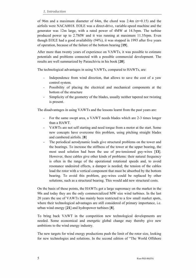
1. Introduction
5 Risø-PhD-80(EN)
of 96m and a maximum diameter of 64m, the chord was 2.4m (=0.15) and the airfoils were NACA0018. EOLE was a direct-drive, variable-speed machine and the generator was 12m large, with a rated power of 4MW at 14.5rpm. The turbine produced power up to 2.7MW and it was running at maximum 11.35rpm. Even though EOLE had a good availability (94%), it was stopped in 1993 after five years of operation, because of the failure of the bottom bearing [19].
After more than twenty years of experience on VAWTs, it was possible to estimate potentials and problems connected with a possible commercial development. The results are well summarized by Paraschiviu in his book [20].
The technological advantages in using VAWTs, compared to HAWTs, are:
- Independence from wind direction, that allows to save the cost of a yaw control system.
- Possibility of placing the electrical and mechanical components at the bottom of the structure
- Simplicity of the geometry of the blades, usually neither tapered nor twisting is present.
The disadvantages in using VAWTs and the lessons learnt from the past years are:
- For the same swept area, a VAWT needs blades which are 2-3 times longer than a HAWT.
- VAWTs are not self starting and need torque from a motor at the start. Some new concepts have overcome this problem, using pitching straight blades and cambered airfoils. [8]
- The periodical aerodynamic loads give structural problems on the tower and the bearings. To increase the stiffness of the tower at the upper bearing, the most used solution had been the use of pre-tensioned guy-wires [13]. However, these cables give other kinds of problems: their natural frequency is often in the range of the operational rotational speeds and, to avoid resonance undesired effects, a damper is needed; the tension of the cables load the rotor with a vertical component that must be absorbed by the bottom bearing. To avoid this problem, guy-wires could be replaced by other solutions, such as a structural bearing. This would add new structural costs.
On the basis of these points, the HAWTs got a large supremacy on the market in the 90s and today they are the only commercialized MW size wind turbines. In the last 20 years the use of VAWTs has mainly been restricted to a few small market spots, where their technological advantages are still considered of primary importance, i.e. urban wind energy [21] and hydropower turbines [8].
To bring back VAWT in the competition new technological developments are needed. Some economical and energetic global change may thereby give new ambitions to the wind energy industry.
The new targets for wind energy productions push the limit of the rotor size, looking for new technologies and solutions. In the second edition of “The World Offshore
1. Introduction
6 Risø-PhD-80(EN)
Renewable Energy Report” [22], published by the British Department of Trade and Industry, VAWT has been pointed as a possible solution for large wind turbines:
“The idea of large megawatt VAWTs is an interesting one […] Lower levels of blade stress occur on VAWTs as opposed to their horizontal counterparts, therefore allowing them be built to a higher capacity. Cost is obviously a key issue and even now it is believed that above 5 MW, large capacity VAWTs could prove to be more cost effective than their traditional tribladed horizontal cousins”
VAWT could be then a candidate for next generation offshore wind turbine, larger than 5MW.
Meanwhile, offshore wind industry is struggling to solve other logistic issues, often independent from the selected turbine. One of the most challenging problems is the erection of wind turbines in deep waters. It is commonly accepted that for offshore sites deeper than 50m, the floating platforms are more economical convenient than the monopoles, used for shallow waters [23], [24], [25].
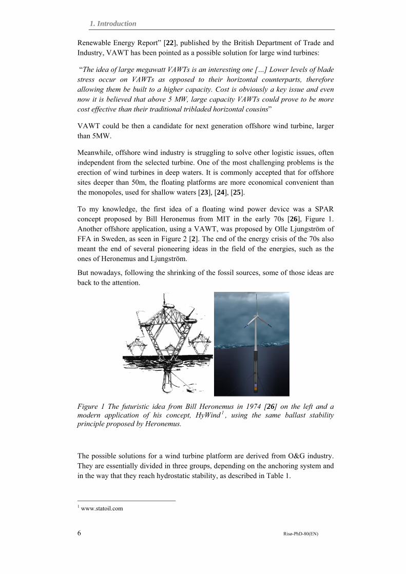
To my knowledge, the first idea of a floating wind power device was a SPAR concept proposed by Bill Heronemus from MIT in the early 70s [26], Figure 1. Another offshore application, using a VAWT, was proposed by Olle Ljungström of FFA in Sweden, as seen in Figure 2 [2]. The end of the energy crisis of the 70s also meant the end of several pioneering ideas in the field of the energies, such as the ones of Heronemus and Ljungström.
But nowadays, following the shrinking of the fossil sources, some of those ideas are back to the attention.
Figure 1 The futuristic idea from Bill Heronemus in 1974 [26] on the left and a modern application of his concept, HyWind 1 , using the same ballast stability principle proposed by Heronemus.
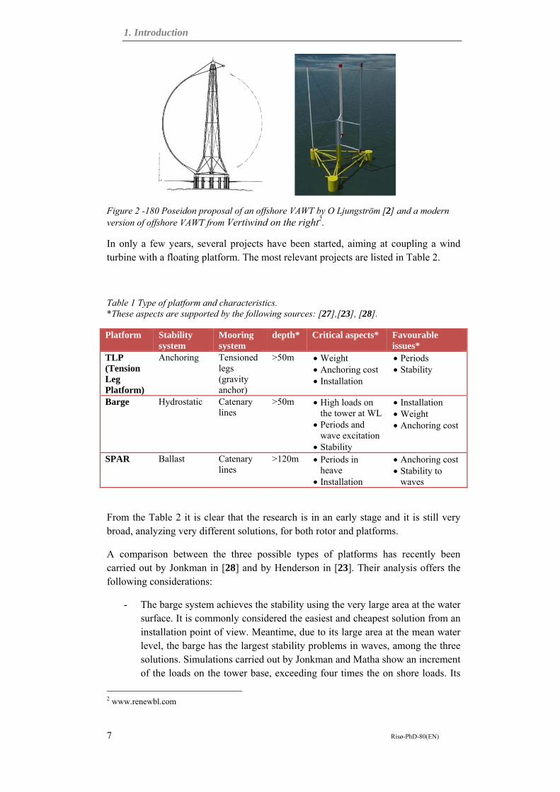
The possible solutions for a wind turbine platform are derived from O&G industry. They are essentially divided in three groups, depending on the anchoring system and in the way that they reach hydrostatic stability, as described in Table 1.
1 www.statoil.com
1. Introduction
7 Risø-PhD-80(EN)
Figure 2 -180 Poseidon proposal of an offshore VAWT by O Ljungström [2] and a modern version of offshore VAWT from Vertiwind on the right2.
In only a few years, several projects have been started, aiming at coupling a wind turbine with a floating platform. The most relevant projects are listed in Table 2.
Table 1 Type of platform and characteristics. *These aspects are supported by the following sources: [27],[23], [28].
Platform Stability system
Mooring system
depth* Critical aspects* Favourable issues*
TLP (Tension Leg Platform)
Anchoring Tensioned legs (gravity anchor)
>50m Weight Anchoring cost Installation
Periods Stability
Barge Hydrostatic Catenary lines
>50m High loads on the tower at WL
Periods and wave excitation
Stability
Installation Weight Anchoring cost
SPAR Ballast Catenary lines
>120m Periods in heave
Installation
Anchoring cost Stability to
waves
From the Table 2 it is clear that the research is in an early stage and it is still very broad, analyzing very different solutions, for both rotor and platforms.
A comparison between the three possible types of platforms has recently been carried out by Jonkman in [28] and by Henderson in [23]. Their analysis offers the following considerations:
- The barge system achieves the stability using the very large area at the water surface. It is commonly considered the easiest and cheapest solution from an installation point of view. Meantime, due to its large area at the mean water level, the barge has the largest stability problems in waves, among the three solutions. Simulations carried out by Jonkman and Matha show an increment of the loads on the tower base, exceeding four times the on shore loads. Its
2 www.renewbl.com

1. Introduction
8 Risø-PhD-80(EN)
potential seems to be mostly restricted to sites where met-ocean conditions are favourable, i.e. a bay rather than open ocean. However some improvements seem to be possible, using a tri-floater configuration, as in the Norwegian project WindSea and in WindFloat from the US. In this project the stability is improved with a novel system of pumps, moving water between the three columns [29].
- The TLP has been, so far, the most exploited concept. The stability is obtained with tensioned cables anchored to the sea bed. Jonkman and Matha show that a turbine mounted on this platform experiences loads very close to the on-shore configuration. On the other hand, the turbine has the largest value of displaced water among the three selected configurations and installation would be challenging, especially because of the anchors. Above that Henderson and Witch notice that in case of failure of one of the wires, the turbine would flip and it would probably collapse in the water.
- The SPAR aims at exploiting deepest sites, at least 120m, as aimed by HyWind [30]. SPAR strength points are in its simple and reasonable light design and in the low wave loads due the small section at the water surface level. In their simulations, Jonkman and Matha found loads similar to the TLP platform, a part from slightly higher bending moments at the tower bottom. Henderson and Witch notice that, contrary to TLP, the failure of one of the anchors would not affect dramatically the stability of the platform. However, they emphasize the challenges connected with installation of such a platform, at sites where a vertical installation (used for HyWind prototype) would not be possible. Indeed in this case the turbine should be towed-out horizontally and then tilted up. This procedure may cause severe loads on the structure, due to the gravitational loads of the rotor and the nacelle mounted at the tower top. During analysis of HyWind concept, Larsen pointed out also a resonance problem due to the interaction of one of the floating natural frequencies (which are very low) with the pitch control of the turbine [33]. He solved the problem by using an adapted control system, whose lowest control-structure natural frequency is lower than the lowest resonance frequency of the tower. Nevertheless, this type of interaction is probable to occur in such kind of constructions and they have to take into account during the design phase. Eventually, Henderson emphasizes also the small design space for such a turbine, due to the many restrictions on the design parameters. An alternative SPAR design, using a tensioned leg anchoring system, was proposed and investigated with a fully coupled dynamic analysis by Withee [34].
Another comparative analysis of SPAR and TLP systems has been presented by Lee and Sclavounos in 2005 [35], who conducted a numerical stability investigation mounting a 5MW HAWT on the two platforms. The results did not show any instability and the authors believe that both the concept would have technological potentials.

1. Introduction
9 Risø-PhD-80(EN)
Table 2Projects on floating offshore wind turbines
Project Name Partner Leader
Status and target of the of project
Platform Rotor
DeepWind Risø Paper/ Academic SPAR VAWT
HyWind [30] Statoil, NO Demonstration / Commercial
SPAR HAWT
MIT/NREL TLP [31] MIT/NREL, US
Paper/ Academic
TLP HAWT
JOIA SPAR [32] JOIA (Japan Ocean Industries Association)
Paper and Prototype / academic and commercial
SPAR HAWT
BLUEH 3 BLUEH, UK Prototype/ Commercial
TLP HAWT
VERTIWIND4 Technip, FR Paper /Commercial TLP VAWT ITI Energy barge [31] Glasgow
University, UK
Paper/ Academic
Barge (squared semi-submerged platform)
HAWT
WindFloat5 Principle Power, US
Paper /Commercial Barge (tri-floater jacket)
HAWT
WindSea6 Statkraft, NO
Paper /Commercial Barge (tri-floater jacket)
HAWT
Sway7 Sway, No Demonstration/ Commercial
Spar HAWT
1.2.3 Numerical tools for floating VAWTs
The development of numerical codes for investigation of the performances of VAWTs started in the 70s. It is possible to distinguish between two groups of numerical methods:
- The BEM codes (based on the Blade Element Momentum theory), also known as stream-tube codes. They are based on the disk actuator theory, imposing the total forces on the blade to be equal to the change in momentum of the stream flow passing through the rotor. The main advantage of this model is the very fast computational time. On the other hand, the code has low accuracy at high tip speed ratio (low rotational speeds) and high solidity.
- The vortex codes, usually based on the Biot-Savart formulation of the vorticity. Their results are commonly considered to be more accurate. Their
3 http://www.bluehgroup.com
4 http://www.technip.com/en/press/technip-launches-vertiwind-floating-wind-turbine-project
5 http://www.principlepowerinc.com/products/windfloat.html
6 http://www.windsea.com
7 http://sway.no

1. Introduction
10 Risø-PhD-80(EN)
use is limited by high computational time and convergence problems at low tip speed ratio.
The first BEM codes were using a single stream tube comprehending the whole rotor. Strickland improved the accuracy with the multi-streamtube formulation, [36]. He divided the rotor into many different stream-tubes, allowing to evaluate the variation of the flow in the two direction perpendicular to the direction of the flow. A further improvement to the model has been carried out by Paravischivoiu, who added another actuator disk to the model, considering the different induced velocities in the upstream and downstream part of the rotor [20].
Another development was achieved by Madsen [37], replaced the plane actuator disk with an actuator cylinder. In this way the velocity field is dependent from the all three directions and not only the two perpendicular to the stream, as in Stricklands dissertation [36].
The BEM codes are mainly used, because of their rapidity, in development of aero-elastic codes. That is also the case for the most used software for simulating offshore floating wind turbines. There are at least a few codes, which couple the aero-hydro-dynamics of the system platform-wind turbine.
At Risø DTU, a hydrodynamic module has been integrated in the aero-elastic code HAWC2, [33], [38], [30]. HAWC2 uses a multi-body formulation, allowing the user to model each component of the turbine as a separate body. The implementation of each body is carried out adopting a finite element theory. The code will be further described in Chapter 6.
Software, currently available for the simulation of fully coupled dynamics of floating wind turbines, has been part of a comparative program under the IEA organization [39].
1.3 Thesis outline Based on this status of the art, I outline my work to solve the proposed objectives.
First of all, in chapter 2, I describe the concept as presented in 2009 and 2010 [1], [40]. I describe the components, justifying their choice in a global design context, bearing in mind that the main goal is to investigate the concept feasibility, rather than its optimization. I dedicate the last part of the chapter to the differences with the former VAWT technology, arguing how some of the typical VAWTs limitations are overcome in this new concept.
The design of an offshore floating wind turbine involves both aerodynamics and hydrodynamics. Then in Chapter 3 I introduce the problem of the floating bodies in the time domain, as formulated by Faltinsen [27] and Newman [41]. My objective is not to have a full comprehensive set of equations, since I will later use a numerical code including an accurate formulation of the floating problem. My objective in this chapter is instead to develop a simplified model to utilize as a preliminary tool for the design of the turbine and the platform. In this model the aerodynamic loads are considered as an external force exciting the system.

1. Introduction
11 Risø-PhD-80(EN)
The DeepWind concept has a peculiarity with respect to the other platforms so far used for wind turbines: the platform is integrated in the tower rotor and it is rotating in the water. Because of this feature, the platform will be loaded with additional external hydrodynamic loads. Indeed a cylinder rotating in a fluid stream experiences a lift force (known as Magnus effect) and a drag force, whose intensity depends on the rotational speed, the radius and the stream velocity. Additionally, a friction moment too acts on the cylinder. Due to the very high Reynolds numbers of a DeepWind MW design, there is not enough literature on this topic. In Chapter 4 I present a study on the forces, conducted with Frederik Zahle at Risø DTU and mainly based on the paper presented at the OMAE conference in 2010 [42]. The results are limited to a few data. However, the values of Cl are very high (up to 10.4) and the Magnus effect needs to be added to the loads in the floating model formulation. Eventually, another aspect needing further investigation is whether and in which magnitude the rotation would alter the flow regimes around the cylinder. This alteration may indeed affect the dependency of the platform behaviour from the no-dimensional numbers commonly used in hydrodynamics.
One of the preliminary aspects in the design and evaluation of the concept is to evaluate the right size for the wind turbine. I decided to adopt a 5MW design as a baseline model. At the present time, this would be a realistic magnitude for a new offshore wind turbine. Additionally, it is also the rated power of the NREL 5MW baseline HAWT defined in [43]. This turbine is broadly used as a reference turbine for offshore platform investigations and it has also been used on a SPAR buoy, recalling the HyWind design, [44]. Even though the size of DeepWind baseline turbine is 5MW, the concept demonstration has to pass through the design of a much smaller demonstrator, as suggested in [3]. Then in Chapter 5 I focus on the challenges connected with the downscaling of the concept from MW to kW size.
My numerical simulations of the concept are mainly conducted with the hydro-aero-elastic code HAWC2, developed at Risø DTU. The code has been used to design the HyWind concept and to simulate other floating wind turbines. HAWC2 has also been selected along with other codes, for a code-to-code verification under Subtask 2 of the International Energy Agency Wind Annex XXIII. [39]. Even though the code has been developed for HAWTs, it has a multi-body formulation, allowing in principle any type of geometry. In chapter 6, I describe the necessary additions to the code, in order to be able to simulate numerically the concept. My work has mostly regarded the development of appropriate computer codes to simulate the aerodynamic loads on each blade element, the control of the rotational speed of the generator and the hydrodynamic loads and friction due to the rotation of the platform.
The chapters 3-6 give the necessary tools to design the floating VAWT. In the chapters 7, 8 and 9 I present the study of three possible sizes, 1kW, 2MW and 5MW. The work is divided in three sections, including the design specifications, the results from numerical simulations and a discussion on the results.
As a result of my work, in Chapter 10 I present an evaluation of the concept and a rough comparison with another floating wind turbine which uses a SPAR platform. Since my study is based on several simplifications, a realistic complete comparison
1. Introduction
12 Risø-PhD-80(EN)
between the two concepts is not possible. Therefore beyond my evaluation, I added some considerations on the possible strategy to obtain a useful tool to compare offshore floating concept.
In Chapter 11, I wrap up my work and I propose some recommendations for the further development and verifications of floating VAWTs with rotating platform.
1.4 Design approach There are two possible approaches to start the design of a floating wind turbine:
- A floating turbine is a very robust turbine mounted on a platform, which need to be stable enough to not create problems to the turbine operations.
- A floating turbine refers to the problem of a complex type of platform, on which additional aerodynamic loads are acting.
Both the two sentences are fundamentally right and they reflect the approach to the problem commonly used by people with different backgrounds, i.e. wind energy or offshore industry.
In this work, my aim is to have an approach to the DeepWind concept that is an integration of the two philosophies above. That requires an iterative process in the evaluation of the concept, which would ideally bring us not to the best rotor neither to the best platform, but to the best integrated system. However, since the main objective of my thesis is the feasibility rather than the optimization, some of the design choices are primarily based on their proven reliability.
There are several constraints in designing a floating VAWT with a spar platform. I grouped them in three groups:
- Structural constraints, limiting the loads on the structure. - Stability constraints, consisting in maximize the natural periods (to avoid the
dominant wave periods), increase the stiffness in pitch and in heave. - Cost constraints, addressing a general reduction in the mass of the structure.
The most relevant dependency of the design from these constraints are shown in Figure 4, following the design philosophy described by Henderson [23]. Several design parameters have a multiple dependency from different requirements, showing the necessity of an iterative and integrated design process. The conflicting requirements reduce significantly the concept design space, as shown in Figure 3, where the simplified case of the design of a spar buoy support structure with constant section is illustrated. The design space is limited by different constraints, which make not feasible many values of the draft and of the radius of the platform. The resulting blank area is the available space for designing the spar buoy. In fact the design is more complex, because of a larger number of variables and constraints and the resulting geometry of the spar buoy is more complex.
My approach to solve this problem is described in Figure 5. The process starts from the fixed external conditions at the selected site, including wind, waves and currents. I consider a shear effect for the wind and the currents but I don’t consider the

1. Introduction
13 Risø-PhD-80(EN)
turbulence effects. Linear theory for regular waves is used to model the oscillatory flow.
The external conditions are transferred to:
- The aerodynamic module, consisting of a BEM code. I used the code to select the dimensions of the rotor (chord, length and diameter) and to calculate the aerodynamic loads on the tower. Considering the bending and the torsion moment applied on the structure, I dimension the cross section of the tower at the mean water level.
- A wave module, to calculate the wave-induced loads on the structure, knowing the dimensions of the tower at the water surface.
- A current module, to compute the loads on the rotating platform, including lateral force (Magnus effect), drag and friction.
All the loads converge to the design of the SPAR platform, taking into account the stability of the system in a steady state (hydrostatic equilibrium) and the resonance frequencies of the system. The wave-induced loads are recalculated with the values of the underwater structure, using an iterative process.
The design obtained with this simplified model is used as input in the aero-elastic software. The verification on the design includes: structural strength and deformations; verification of the maximum loads; verification of the natural periods; stability of the system in terms of tilt angle and maximum displacements.
The process is iterated until the design is acceptable.
Radius of the platform [m]
Dra
ft o
f th
e p
latfo
rm [m
]
Stiffness in Pitch (C55)
Cost Structural strengthHydrodynamic loads (Magnus effect)Heave Period (Tn3)
Friction
Figure 3 Design space area for the rotating supporting structure of a floating VAWT.

1. Introduction
14 Risø-PhD-80(EN)
Figure 4 Most relevant design drivers and constraints
Benefits in increasing the design variable
Benefits in decreasing the design variable
Variables of the design
Stability drivers (to maximize)
Structural constraints (to reduce)
Surface section area (Aw)
Draft of the platform (HP)
Rotor Rotational
speed ()
Max Radius platform (RP)
Natural periods of the platform (Tn3, Tn4)
Wave induced loads (diffraction + radiation)
Torque on the shaft (Q)
Magnus effect and friction (Fl, Mf)
Hydrostatic restoring in pitch (C44)
Hydrostatic restoring in heave (C33)
Cost reduction
Platform Weight (W)

1. Introduction
15 Risø-PhD-80(EN)
Figure 5 Design layout
External conditions: Wind Waves Currents
Aerodynamics (DDMST): Performances Aerodynamic
Loads Dimension of
the rotor
Tower design: Dimensions Weight
distribution
Platform design: Dimensions Weight
distribution
Loads from currents: Lateral force Drag Friction
Wave-induced loads: Hydrodynamic Diffraction Radiation Viscous effects
Verification (HAWC2): Extreme loads Period
verification Maximum
Displacements
Final design

2. DeepWind concept
16 Risø-PhD-80(EN)
2 DeepWind concept 2.1 Main concept description This work regards the concept shown in Figure 6 and described in [1]. The design consists of a Darrieus rotor, whose tower is extended underwater, in order to act as a spar buoy. The whole system is rotating and generates power with a generator placed at the tower bottom and fixed at the anchoring system.
The water is working as a rolling bearing, damping the dynamic effects of the bending moment on the turbine.
Figure 6 Artistic view of the concept
Before starting the description of the components, a clarification is needed. At the present stage the design of the concept has two purposes: demonstrate the feasibility of the concept and create a baseline model to test technological improvements. Therefore the number of uncertainties in the design has to be limited to the minimum and proven technologies should be used, when possible. This approach will justify most of the technological choices on the components described in the next paragraphs. A similar approach has been used by Hendricks [45] for the design of the baseline 6MW HAWT, included in the DOWEC project.
2.2 Components
2.2.1 Rotor The rotor is a vertical-axis wind turbine. The Darrieus rotor has been selected among the many design solutions proposed for VAWTs in the past years. The reasons for this choice are:
- The simplicity of the concept design, that is at the basis of the entire design. Darrieus rotor gives better up-scaling potential and it matches with the other components described in the next paragraph (i.e. blades and control system).
2. DeepWind concept
17 Risø-PhD-80(EN)
- The possibility of using blades with Troposkien shape, which can reduce the bending moment on the blades due to the centrifugal force [9], [20].
- The reasonable efficiency of the Darrieus rotor, rated to Cp around 0.4 and close to the values reached with HAWTs [20].
- The long record of research and development in the past years, as mentioned in Chapter 1. The acquired experience on this rotor can facilitate the feasibility evaluation of the concept.
2.2.2 Blades The blades for a Darrieus rotor, as in Figure 6, are between two and three times longer than a HAWT of the same rated power [20]. The length can be reduced using straight blades, but then the rotor would additionally need some connection arms. Eventually, curved blades have been selected also considering the possibility of Troposkien shape, as previously mentioned.
The blades for a VAWT are characterized by a simple design and in principle they can be produced with a constant geometry along the length, without tapering. This allows the use of pultrusion for the manufacturing process, that would allow a significant reduction in the costs [46]. The pultrusion process of GRP seems quite promising for large blade profiles, and the material strength of pultruded GRP is much better than for hand layed-up GRP for horizontal-axis wind turbines. Migliore estimates a reduction in the manufacturing costs around 50 and 74%, that would permit to produce blades for VAWTs at competitive cost (compared to blades for HAWTs).
2.2.3 Generator There are a few solutions to generate power using the torque transmitted to the bottom of the platform. Some solutions are presented in the concept description in [1].
Here I will focus on three solutions using a generator placed in the bottom of the submerged structure.
The configurations are:
The generator is mounted inside the submerged foundation at the bottom and rotates with the rotor. The shaft is extended through the foundation bottom and fixed to the torque arms, Figure 7-a.
The generator is mounted outside the foundation and fixed to the torque arms. The shaft is fixed to the torque arms, Figure 7-b.
The generator is fixed on the sea bed and the shaft is fixed to the rotating structure, Figure 7-c.

2. DeepWind concept
18 Risø-PhD-80(EN)
Figure 7 Possible configurations for the generator
Additionally the generator is used for two other tasks:
- it must work as a motor to start the Darrieus rotor, since this kind of turbine is not self starting.
- it has to operate at variable speed to control the turbine operations.
2.2.4 Anchoring The torque and the thrust are transmitted through the tower to the bottom of the structure. The platform is anchored to the sea bed with a catenary mooring system. The forces are transferred through the mooring lines, but to take the torque two or more rigid arms are necessary, as seen in Figure 8.
Figure 8 Torque arms to connect the rotor to the anchoring system, dimensions of the arms are exaggerated for visualization
A solution involving other types of anchoring system, such as the tensioned wires proposed by Withee [34], is not suitable due to the high values of the torque to be absorbed. Another limitation regards the point to connect the anchoring system. In a similar concept for HAWTs, i.e. Hywind [30], the mooring lines are attached on the platform above the centre of gravity. In this concept, this is not possible because the platform is rotating and this solution would require a big and expensive bearing. Therefore the mooring lines are attached at the bottom of the platform and they do not give contribution in restoring the turbine in pitch and roll.
When the generator is placed on the sea bed, as in Figure 7-c, the mooring lines are not needed and the torque is transferred directly to the ground.
2.2.5 Safety system The VAWTs are weaker than HAWTs in avoiding overspeeding conditions. Indeed the most common HAWTs are nowadays pitch controlled and can use aerodynamic brakes in addition to a mechanical system. VAWTs need a big mechanical brake

2. DeepWind concept
19 Risø-PhD-80(EN)
system at the bottom of the structure, sometimes consisting of two brakes, one on each shaft (low and high speed), [2].
For a floating VAWT, water brakes can be used as overspeeding protection. The system consists of drag devices, deploying from the rotating submerged foundation in case of overspeeding conditions, Figure 9.
Figure 9 Sketch of the water brakes system
2.2.6 Control strategy Compared to a HAWT, the rotor does not need a pitch neither a yaw control system. The power control is obtained by rpm control of the rotor speed [17]. Also this solution allows a simple design and it is in principle favourable for up-scaling purposes.
A control based on the rotational speed has also some limitations, bringing severe periodical loads on the generator connection.
2.3 Strategies for installation and operation and maintenance
2.3.1 Installation The rotor and the foundation can be towed to the site. In case of a two-bladed rotor, the whole structure, without counterweight, can float and lay horizontally on the water line. Counterweight can be gradually added, to tilt down the turbine. In case that the generator is mounted inside the foundation, it can be inserted from the top of the structure. This is a typical installation in O&G industry and it would be more favourable than for HAWTs, because the lower weight at the top of the tower would reduce the bending moment on the structure during the procedure.
2.3.2 Operation and Mantenaince (0&M) Some specific solutions are available for the maintenance of the turbine.
Moving the counterweight from the bottom of the foundation upwards is possible to tilt up the submerged part for service. An outside generator can be serviced and marine growths on the rotor can be removed.

2. DeepWind concept
20 Risø-PhD-80(EN)
In case of internal arrangement of the generator, it is possible to place a lift inside the tubular structure to have easy access from the top of the turbine to the submerged part.
2.4 Concept potentials The most obvious advantage of the concept is its simple design. The whole construction is simply a rotor, embedded in and supported by the water itself. Another example of the simple concept is the blades. Rather large blade sections can be pultruded in GRP by production facilities that are indeed rather small. In principle, a production facility can be put on a ship, and the blades can be produced offshore in lengths of kilometres. Otherwise the blade could be manufactured at the harbour avoiding the limitations connected with on land transportation.
Another advantage is in the control system. It needs no yawing system to position the rotor into the wind and no pitching of blades is necessary to regulate power. The Darrieus rotor is stall-regulated at high wind speeds, or the power can be down-regulated by reducing the rotor speed. Over-speeding protection can be made very efficient and small using water brakes.
An advantage of the concept is that the rotor may be tilted by moving the ballast in the tube, during installation and maintenance.
2.5 Specific challenges In [1], the most important challenges have been pinpointed, which need to be investigated in order to validate the feasibility of the concept.
The rotating tower is subject to hydrodynamic loads, due to the interaction to a waterstream. This will create further limitations in the design and it will overload the submerged structure. Moreover there are some losses due to the friction of the platform in the water. This issue addresses special requirements on the platform maintenance, to control an excessive marine growth.
The advantage that the generator with a high mass may be put in the bottom of the rotor tube generates another challenge. The positioning of the generator in the bottom makes maintenance and exchange of the component very complicated. Methods for lifting up the generator through the tube, eventually in smaller parts, must be developed.
Even though the Darrieus rotor was developed significantly during the 70's and 80's it is still considered a challenge to make blades for this design in a cost-efficient way. The most promising method seems to be pultrusion of GRP in full blade length sections that are bent into the blade shape and glued together.
The most significant tower difference compared to the horizontal-axis wind turbine is that the rotor torque must be absorbed in the sub-sea systems. This may be through the use of torque arms connected to the anchoring system or through drag elements in the water. The torque of the Darrieus rotor varies with the position on the rotation and this varying torque will also have to be absorbed through the anchoring system.

2. DeepWind concept
21 Risø-PhD-80(EN)
2.6 Methodology for the investigation of the concept and available configurations
The complexity of the floating VAWT suggests the possibility to decompose the investigation in different steps, based on the number of DOF (degrees of freedom). We decided to develop the concept, investigating three configurations with different DOF. The degrees of freedom of the three configurations are summarized in the table below, the yaw motion is not considered because it is in the direction of the rotational speed of the rotor.
Table 3 Degrees of freedom of the three configurations
Surge Sway Heave Pitch Roll 1st Configuration (Sea bed configuration)
X X
2nd Configuration (Fixed torque arm configuration)
X X X
3rd Configuration (Mooring fixed configuration) X X X X X
2.6.1 First Configuration (Sea bed configuration) The generator is directly fixed on the sea-bed and the shaft is extended to the sea bottom, as in Figure 7-a. The shaft has two rotational degrees of freedom: it can tilt back and forth and to the sides (pitch and roll).
Figure 10 Schematic drawing of the first configuration (sea bed configuration)
This configuration is not fully floating, it has not translational degrees of freedom and the forces are transferred vertically between the rotor and the sea bed. However, the equilibrium in pitch and roll is achieved with the same principle of a moored anchored floating turbine. Also the equilibrium between the buoyancy and the gravity loads is equally necessary, to avoid high loads on the bottom bearings.
The sea bed configuration has been selected to be investigated first, in order to verify that the concept works without serious vibrations and instabilities. Therefore the current work is focused on the study of this configuration.

2. DeepWind concept
22 Risø-PhD-80(EN)
2.6.2 Second Configuration (Torque arm fixed configuration) The generator is mounted on a torque arm. Compared to the sea-bed configuration the shaft has one more translational degree of freedom, i.e. it can move up and down (heave).
Figure 11 Schematic drawing of the second configuration (torque arm fixed configuration)
This configuration has been selected for next test in Roskilde Fjord.
2.6.3 Third Configuration (Mooring fixed configuration) Three torque arms are mounted to the generator box. The torque arms are connected to the sea bed by a mooring system. Compared to the previous configuration the shaft has two more translational degrees of freedom (sway and surge).
Figure 12 Schematic drawing of the third configuration (Mooring fixed configuration)
2.7 Progress beyond the VAWT state of the art Blackwell in 1974 [47] pointed out three reasons to prefer VAWTs technology to HAWTs:
1. Independence of the VAWTs operation from the wind direction
2. Generator placed at the bottom
3. Simplicity of the tower construction.

2. DeepWind concept
23 Risø-PhD-80(EN)
More than 35 years after, those are the same mostly used arguments to bring VAWTs back in the market.
Thus, the question is “why those arguments, which were not good enough forty years ago, should be valid today?”
The goal of this concept is to demonstrate that those arguments can finally make VAWTs competitive, if they are combined with the right new technological development and ideas. In particular, there are two limitations concerning old VAWTs technology, which DeepWind concept aims at overcoming.
The first is the cost of blades that was a serious limitation for VAWT development. The pultrusion process had made strong progresses compared to forty years ago. Its use has already been considered for HAWTs, for the high cost reduction in the production, [46]. So far this solution has been limited by the shape of the blades for HAWTs, which need to be tapered using different airfoils. For VAWTs pultrusion represents an important improvement over one of the most relevant limitations of their design.
The second novelty concerns the use of guy wires or of costly bearings, which were affecting the cost-effectiveness of VAWTs. DeepWind design uses the water as a roller bearing, aiming at preventing severe vibration on the tower and avoiding bearings above the sea water. The idea to use the ocean as a bearing is common to another concept, developed in Sweden8, called SeaTwirl. The developer of this other concept claims to have conducted studies at Gothenburg Univeristy, proving the feasibility of the use of the water as a bearing.
8 http://seatwirl.com
3. Loads and dynamics of a floating vertical axis wind turbine
24 Risø-PhD-80(EN)
3 Loads and dynamics of a floating vertical axis wind turbine
3.1 Formulation of the problem The design of a floating VAWT is driven by two types of parameters:
- Structural endurance to the loads (ultimate strength and fatigue). - Dynamic stability of the system, stability of the structure and of the motion
(translational and rotational)
In this chapter I introduce the loads acting on the turbine and the corresponding dynamics. A few clarifications are needed:
- I use a simplified model, aiming at having a general insight into the concept and to identify the most relevant parameters for a pre-design of the concept, see Figure 5. I will introduce in the following paragraphs the needed assumptions for the respective simplifications.
- When it is in a water stream, the turbine experiences some specific hydrodynamic loads, due to the rotation of the foundation. Considering the novelty of these loads on a wind turbine, I have chosen to discuss the currents-induced loads in a broader way in a separate chapter (Chapter4). However these loads can be added to the equation of the dynamics as further external loads.
An offshore floating turbine is subject to higher loads than on land. Therefore more robust structures are commonly used to dimension the structure. However the real challenge in the design of these machines is to integrate the rotor design in the project of the floating platform. The sketch in Figure 13 shows the different aerodynamic and hydrodynamic loads acting on the system. The reaction forces of the anchoring are not included in the figure and I will not consider them in my further discussion.
The met-ocean conditions are described using the concept of sea state. A sea state is a statistical description of the met-ocean conditions at a site with respect to waves, and it is described with the significant height Hs, the peak period TP and the power spectrum. Joint description of currents and wind can be added to the sea state. The sea state varies with the time, but in the formulation I will use in the next sub-chapters, the sea state is supposed to be a stationary random process. This is a reasonable assumption for the relative short periods used for averaging statistical met-ocean data (i.e. one hour) and for the length of the time series of steady state numerical simulations.

3. Loads and dynamics of a floating vertical axis wind turbine
25 Risø-PhD-80(EN)
Figure 13 Simplified sketch of the loads acting of the floating VAWT. Magnitudes and directions are not fully indicative of the real loads. Wind speed is defined along the y-axis
In this chapter, I consider the floating turbine as a rigid body having six degrees of freedom, corresponding to the three rigid translations and three rigid rotations, respect to the three axes. The six types of motion are described in Figure 13 and Table 4. As emphasized in Table 4, the most critical motions for a SPAR platform are the displacement on the z axis (heave) and the rotational modes around the x and y axis (pitch and roll).
Figure 14 Degrees of freedom for a floating VAWT
In other references, as [27], the pitch motion is described as the motion around the y-axis. My choice is to select the pitch as the motion generated by the aerodynamic thrust (the wind direction is selected on the y-axis in the numerical solver).
The z-axis is often pointing upwards in other studies, also this choice is made to be consistent with the reference system of the numerical solver.
Wsp: Wind speed
U: Water current speed
A, T: wave amplitude and period
T: Aerodynamic force on the rotor (thrust and side force)
Q: Aerodynamic torque
L: Hydrodynamic side force, perpendicular to the water current direction
Fm: Hydrodynamic forces in oscillatory flow (Morrison formulation)
Mf: Friction Moment

3. Loads and dynamics of a floating vertical axis wind turbine
26 Risø-PhD-80(EN)
Table 4 Definition of the DOF of a floating VAWT
Index DOF Displacement Critical for spar system
1 Surge translation on the x axis [m] No
2 Sway translation on the y axis [m] No
3 Heave translation on the z axis [m] Yes
4 Pitch rotation around the x axis
[degrees] Yes
5 Roll rotation around the y axis
[degrees] Yes
6 Yaw rotation around the z axis
[degrees] No
A floating body has three main types of motion
- Wave-induced motion: Induced by the hydrodynamic loads in an oscillatory flow, as I will discuss accordingly to the linear potential theory and the Morison’s formulation.
- High frequencies motion: it mainly occurs at resonance conditions. It is a common design procedure, to dimension the structure in order to have natural periods out of the range of dominant wave frequencies. However resonance conditions can occur to the second order non linear wave conditions
- Drift motion: it consists of the translational motion (main drift) and its second order components (slow-drift). It can be generated by external loads, such as from wind and currents, or by second order non linear effects.
In chapter 3 I only consider the wave-induced motion, disregarding non linear effects and supposing the displacements of the turbine to be small.
Apart from the waves, the other external loads acting on the turbine (i.e. aerodynamic and water currents loads) will be added as further external loads in the equation of the motion. The problem will then describe the wave-induced motion of a floating VAWT, subject to aerodynamic and current loads.
3.2 Aerodynamic loads on a two bladed VAWT I consider the aerodynamic loads on the turbine, as the total aerodynamic forces and moments acting on the tower. In this simplified model, I will disregard the inertial loads deriving from the centrifugal force.
All the aerodynamic loads on a VAWT are periodical, as shown in the VAWT introduction in Chapter1. The amplitudes and the periods of the oscillations depend on the number of blades. A three bladed rotor is characterized by more regular loads and lower periods. The plot of the thrust force on the tower presents three low and quite broad peaks in a revolution.

3. Loads and dynamics of a floating vertical axis wind turbine
27 Risø-PhD-80(EN)
On the opposite, the thrust produced by a 2 bladed rotor has 2 high and sharp peaks per revolution. In this chapter I will consider the aerodynamic loads from a 2 bladed rotor, following the design of chapter 2.
The basic aerodynamic loads to dimension a VAWT are:
- The longitudinal force in the wind direction (thrust) Ty:
cos 2
is the component of the aerodynamic force in the y direction is the
variation in a revolution, is the half rotational frequency of the rotor
(corresponding to the period needed for a blade to cover an arch of 180
degrees), .
- The transverse force perpendicular to the wind Tx:
cos 2
- The torque
cos 2
For a two bladed rotor, which is the design considered in this work, the following applies:
~ ~
~
Where ~ indicates the same order of magnitude.
These equations express a useful approximation, describing the relevance of the periodical components, in the loads on a 2 bladed VAWT.
The aerodynamic forces can be divided in two halves and applied on the rotor as in Figure 13, generating a moment Mb on the tower, having its maximum value on the cross section at the mean surface level. These loads are useful here, to define the external loads in the equations of the motion of the floating body.
Additionally the loads are used to calculate the maximum stress on the turbine. Compared to a HAWT, the tower of a floating VAWT is subject to a lower stress
from Mb, , due to the lower height of the centre of the rotor. On the other
hand the tower is loaded with an additional torsion moment, generated from the
reaction of the generator, corresponding to a stress on the external surface
of the cylinder. (With RT external radius of the tower, IP polar moment of inertia of
the section and stress on the surface of the tower).

3. Loads and dynamics of a floating vertical axis wind turbine
28 Risø-PhD-80(EN)
3.3 Wave-induced loads
3.3.1 Formulation of the problem and assumptions There are different possibilities to investigate the steady-state wave-induced loads on a floating body. Here, I use the academic theories based on a frequency-domain approach and I write the resulting equations in the time domain. A more detailed description of these theories can be found in [41], [27] and [48]. An alternative approach to the wave-induced problem is reported by Jonkman [31], where he described the “true linear hydrodynamic model”.
All the references above use the linear theory of the wave propagation to solve the equations of the motion of the floating body. This means that the loads and the
motions induced by the waves are proportional to the wave amplitude, a. This
assumption is acceptable for sea states far from the breaking wave limit, i.e. for aw
sufficiently small, where w is the wavelength.
Under the linear theory it is possible to apply the superposition of the effects. The hydrodynamic loads on a platform in oscillatory flow (excluded the loads due to currents) are then composed of three contributions:
- Hydrostatic loads, which are present independently from the waves and consisting of the buoyancy and the restoring terms (excluded the restoring from external forces, such as the reaction force of the mooring lines).
- Diffraction loads, corresponding to the loads on the body, when this is supposed to be fixed in an oscillatory flow. They consist of scattering wave loads and the Froud-Krylov force and moment.
- Radiations loads, due to the waves irradiated from the body, when the body itself is forced to oscillate (in each of the six DOF) in steady water at the same frequency of the exciting waves. They are composed of added mass (inertial) and damping (viscous) loads.
In my simplified model, I calculate the diffraction and radiation loads using the potential theory. Then to estimate the viscous terms, disregarded by the potential formulation, I use the Morison’s equation.
3.3.2 Regular waves and statistical description Some additional assumptions are necessary to apply the potential theory: the fluid is supposed to be inviscid and incompressible and the motion is irrotational. Under
these conditions it is possible to find a velocity potential function , that satisfy the
Laplace equation: 0.
A velocity potential is obtainable imposing four boundary conditions: the body surface is supposed to be impermeable, imposing the normal velocity equal to zero; the same conditions is applicable at the sea bottom equalizing the vertical velocity to zero; the water pressure at the sea surface is equal to the atmospheric pressure (free surface dynamic condition) and the fluid particle on the free surface will continue to
belong to the same surface ( =0, kinematic free surface condition).

3. Loads and dynamics of a floating vertical axis wind turbine
29 Risø-PhD-80(EN)
It is possible to demonstrate, [41], that a solution of Laplace equation that satisfies the four conditions is:
Φ cos Eq.1
Where k=2 is the wave number and w is the circular wave frequency; the waves are propagating in the x direction and the z axis is oriented downwards, as in Figure
14. Here, the water depth is considered infinite, represents the potential function of a two-dimensional plane progressive regular wave system, propagating along the positive x direction with the surface elevation described by the equation:
sin
For finite water depth (h), the equation Eq.1 becomes:
Φ
cos , with k satisfying the identity
tanh
Integrating the potential function, it is possible to derive the equation of the free
surface , the velocity and the acceleration of the water particles and the dynamic pressure pD.
The description of random irregular waves is achievable by superimposing multiple regular waves. The free surface of an irregular wave propagating on the x axis is obtainable by superimposing the amplitudes of N regular waves:
∑ sin ,
With 0j the phase angle of the j wave.
The values of each amplitude aj are related to the wave spectrum at a particular site. The most used wave spectrum is the JONSWAP (Joint North Sea Wave Project), [48]. The IEC standards for offshore wind turbines [49], recommends the following formulation for the JONSWAP spectrum:
0.3125 exp 1.25 1 0.287 .
In the formula, fP and TP are respectively the peak wave frequency and period, Hs is
the significant wave height, fw the wave frequency, is a shape parameter defined in
the standards depending on the sea state and is a parameter varying with the wave frequency.
For equal to 1, the equation above describes the Pierson-Moskowitz (PM) spectrum. This has a lower and broader peak compared to the JONSWAP spectrum. The standards recommend that PM spectrum is used for fatigue calculations and the JONSWAP to evaluate extreme sea states, as well for shallow water sites.

3. Loads and dynamics of a floating vertical axis wind turbine
30 Risø-PhD-80(EN)
Eventually the IEC standards gives also indications on the calculation of the zero crossing wave periods, to evaluate the range of the significant wave periods, in which resonance is likely to occur [49].
In open-sea conditions, it is commonly used, as range of significant waves, the frequencies interval between:
0.04Hz<fw<0.2Hz,
Corresponding to the periods:
5s<Tw<25s.
3.3.3 Hydrostatic loads The hydrostatic loads consist of the restoring terms, which are proportional to the
displacement i, and of the gravitational loads acting only on the z axis (buoyancy).
, 1,6 1,6
i3 is the Kronecker-Delta function, w is the density of the water, V the displaced
volume of water without considering the effect of displacement i, Cij are the terms of the restoring matrix. The first right-hand term in the equation above is the
buoyancy of the body without considering the displacements i of the body itself. As argued by Jonkman [31], this term is often disregarded, because it is equalized by the total weight of the structure and the anchoring system. Nevertheless to catch the dynamics of the system it is important to evaluate the relative positions of the centre of gravity and the centre of buoyancy. Therefore it is a good practice to decouple the two centers. Moreover from a design aspect, the vertical equilibrium is not given, instead it is an important parameter to adjust during the iterative design process.
The second right-hand side terms are the loads originated by the change in the
hydrostatic forces and moments, subsequently to the rigid displacement i of the platform.
For an axial symmetric body (i.e. a cylindrical platform) the matrix has only five terms not null [27], [31]:
0 0 0 0 0 00 0 0 0 0 0
0 0 0 0
0 0 0 0 0
0 0 0 0
0 0 0 0 0 0
Where, zB and zG, represent respectively the position on the z axis of the centre of buoyancy and of gravity.
The terms in the matrix are:
3. Loads and dynamics of a floating vertical axis wind turbine
31 Risø-PhD-80(EN)
- C33 is the buoyancy, as argued above. - C53=C35 is the restoring moment of the coupled motion heave-roll, due the
action of the water plane area. - C44 and C55 are the restoring terms in pitch and roll. They are composed of
two terms. A moment generated by the relative positions of the centre of gravity and the centre of buoyancy; another moment related to the water plane area. For platform with L>>Aw, such as a SPAR buoy, the first term is dominant over the second.
3.3.4 Radiation loads A system of radiating waves is created by the forced oscillations of the floating body in still water. The loads on the body generated by these waves are the radiation loads:
,
An exact derivation of the equation of Aij is described by Jonkman in [31]. Here, I will refer to the engineered methods introduced in other references [27], [41].
Since these loads are generated by the oscillation of the body, Aij and Bij are dependent on the body shape and on the frequency of the oscillations.
In this paragraph I disregard the terms Bij and I will consider the viscous effect using the Morison’s formulation.
To calculate Aij, the most used method is the strip theory. This consists of integrating the 2d coefficients Aij
2D, calculated for a cross section, along the main length of the body (i.e. the platform length for a SPAR). Newman reports the 2D coefficients of added mass for the most common cross sections [41]
3.3.5 Diffraction loads These are the loads acting on the platform, when it is considered fixed. They are composed of two terms:
- The Froude-Krylov force, which are the loads generated by the undisturbed pressure field, as calculated from the wave potential theory.
- The loads from wave diffraction, caused by the perturbed pressure field.
From the potential flow, for waves propagating in the x axis, the dynamic pressure of a fluid particle in the undisturbed wave field is:
coshcosh
sin
For a slender structure, whose dimension is smaller than the wavelength (for a SPAR
D<<), the diffraction forces are:
, ,

3. Loads and dynamics of a floating vertical axis wind turbine
32 Risø-PhD-80(EN)
Sl is the lateral surface of the platform, Aij are the added mass terms as discussed in the former chapter and aij are the acceleration of a fluid particle according to the potential theory.
3.3.6 Morison’s formulation and the viscous loads and damping Morison found an engineering approximation to express in-line forces induced by the waves on a slender structure, whose diameter is smaller than the wavelength.
Morison’s force acts on the direction of the wave propagation and the value dF on a strip dz of a vertical cylinder, is:
0.5 | | Eq.2
u is the velocity of a fluid particle and is the acceleration.
The first right hand term is the drag force of the radiation problem and CD is the drag coefficient.
The second right hand term is the inertial force and CM is the inertia coefficient.
CM can be expressed as CM=1+Cm, where Cm is the hydrodynamic mass coefficient, that is equal to 1 for circular cylinders [50].
Considering the body moving relative to the flow with velocity ur, the in-line force on a strip dz is:
0.5 | |4 4
The last two right hand terms correspond to the hydrodynamic mass force and the Froude-Krylov force as discussed in the potential flow theory.
The non dimensional coefficients CM and CD can be related to some characteristic parameters of the platform. The most important values to consider to estimate CM and CD are:
Keulegan-Karpenter number: 2
Reynolds number:
Re/KC:
The dependence of the Morison’s coefficients has been largely investigated and it is reported in books [27], [41] and [50]. For instance, the dependence of KC states the existence of two regimes.
At 0<KC<<20-30, the inertial term of the equation Eq.2 is dominant and the cylinder is in an inertia-dominated regime.
At KC>20-30, the wave amplitude is much larger than the characteristic length of the body and the fluid separate from the body’s boundary. At this conditions it is

3. Loads and dynamics of a floating vertical axis wind turbine
33 Risø-PhD-80(EN)
possible to observe a rapid decrease of the inertial term (inertial crisis) and the cylinder is in a drag-dominated regime.
Another important parameter is the ratio w/D and, for w>>D, the first term of equation Eq.2 corresponds to the wave-induced loads calculated with the potential theory.
3.4 Equation of motion and natural periods
Applying Newton’s second law and considering the loads mentioned so far, it is possible to write the equation of the motion for a floating body:
F M Ad ηdt
Bdηdt
C η 1 ,6
The left hand term is the complex amplitude of the external exciting force, i.e. the wave-induced loads. Mij are the terms of the mass matrix that, considering again the symmetry around the plane x-z, is equal to:
0 0 0 00 0 0 00 0 0 0 00 0 0
0 0 0 00 0 0 0
The other terms Aij, Bij and Cij are respectively the added mass, damping and restoring coefficients.
By imposing for the displacements:
And 0
Dividing by , one obtains a system of six equations in the real numbers domain:
1,6 Eq.3
The simplifications above can be justified with the following additional assumptions:
- The floating body oscillates at the same wave amplitude and frequency at every instant
- The coupled effects are disregarded. In case of spar buoys this means in particular not to consider the coupling of the pitch-heave and pitch-roll motions. Once again, I emphasize that I use this simplification only in the simplified model for a pre-design of the platform. The coupled motions are fully taken into account in the aero-elastic simulations with HAWC2.

3. Loads and dynamics of a floating vertical axis wind turbine
34 Risø-PhD-80(EN)
From equation Eq.3, it follows that the equation of the natural periods, for an undamped floating body, is:
2 Eq.4
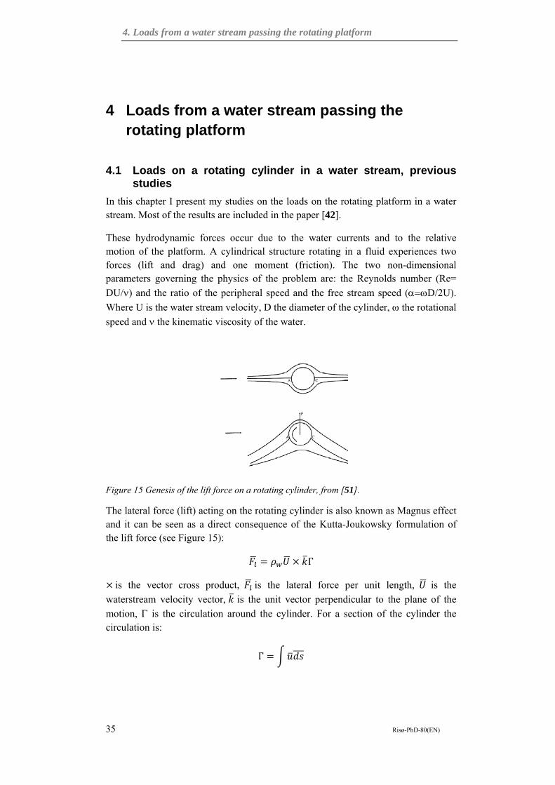
4. Loads from a water stream passing the rotating platform
35 Risø-PhD-80(EN)
4 Loads from a water stream passing the rotating platform
4.1 Loads on a rotating cylinder in a water stream, previous studies
In this chapter I present my studies on the loads on the rotating platform in a water stream. Most of the results are included in the paper [42].
These hydrodynamic forces occur due to the water currents and to the relative motion of the platform. A cylindrical structure rotating in a fluid experiences two forces (lift and drag) and one moment (friction). The two non-dimensional parameters governing the physics of the problem are: the Reynolds number (Re=
DU/) and the ratio of the peripheral speed and the free stream speed (D/2U).
Where U is the water stream velocity, D the diameter of the cylinder, the rotational
speed and the kinematic viscosity of the water.
Figure 15 Genesis of the lift force on a rotating cylinder, from [51].
The lateral force (lift) acting on the rotating cylinder is also known as Magnus effect and it can be seen as a direct consequence of the Kutta-Joukowsky formulation of the lift force (see Figure 15):
Γ
is the vector cross product, is the lateral force per unit length, is the
waterstream velocity vector, is the unit vector perpendicular to the plane of the
motion, is the circulation around the cylinder. For a section of the cylinder the circulation is:
Γ

4. Loads from a water stream passing the rotating platform
36 Risø-PhD-80(EN)
is the integral of the scalar product between the vector (water velocity at the
edge of the cylinder boundary layer) and the vector (element of the lateral surface of the cylinder). If the cylinder is in still water, the circulation is null and there is no force on the cylinder. When the cylinder starts spinning in a viscous fluid, the viscosity creates a circulation around the cylinder and a lateral force on the surface of the cylinder:
The magnitude of the vector per unit length can be written as proportional to the dynamic pressure:
0.5
Where D is the diameter of the cylinder and Cl is the no-dimensional lift coefficient.
The first studies on a rotating cylinder were carried out by Prandt [52]. He stated that
the Cl increases linearly with until an asymptotic value, i.e. ClMax=4, that results from integrating the pressure around the cylinder when the two stagnation points on the cylinder are coincident. In the last 50 years many numerical, theoretical and experimental studies have been carried out, as well summarized by Mittal [53] and Padrino [54].
Unfortunately most of the studies are numerical simulations at low Re (<103) and
low . The typical Reynolds values for DeepWind’s platform are greater than 106. The first numerical study was made by Glauert [55], who solved the two dimensional Navier-Stokes equations. Glauert’s results show that the lift increases
linearly and indefinitely with , exceeding the limit of Prandtl. Other studies show different results: Chew [56] confirms in his numerical studies the results of Prandtl; however the experiments by Tokumaru [57] and the numerical model by Mittal [53] show a value of the lift higher than the limit of Prandtl, even if an asymptotic value
is observed as well. The value of when the vortex shedding ceases and the lift
tends to an asymptotic value is called limit (L).The value of L depends on Re. For very low Re (Re<160) this value is a logarithmic function of Re, for Re>103 it
seems to be constant, i.e. L =2 [53].
Some numerical results at higher Re (104<Re<106) are presented by Chang [58]. The stopping of vortex shedding is shown and the Cl seems to decrease at high Re. Unfortunately, the numerical simulations at high Re are very limited in time because of convergence problems and it is not possible to predict a fully developed regime.
The boundary layer around a rotating cylinder is described by Padrino [54] and Wang [59] for Re<1000. The friction torque coefficient is reported and it seems to decrease by the Re number. Another possibility to calculate the friction of a rotating cylinder at high Reynolds numbers is shown by Theodorsen in [60].

4. Loads from a water stream passing the rotating platform
37 Risø-PhD-80(EN)
4.2 Methodology of the study This study is based on a CFD investigation conducted on a rotating cylinder in a water stream. The diameter of the cylinder and the rotational speeds are consistent with the possible design of a 2MW machine. The simulation is repeated for different rotational speeds, corresponding to the operating conditions of the wind turbine at different wind velocities. The power curve used for this study is in Figure 16, along with the aerodynamic thrust force on the rotor. The dots highlighted in the chart represent the four operating conditions of the rotor presented in this chapter.
wsp [m/s]
0 5 10 15 20 25 30
P [
W]
-5,0e+5
0,0
5,0e+5
1,0e+6
1,5e+6
2,0e+6
2,5e+6
T [
N]
0
1e+5
2e+5
3e+5
4e+5
5e+5
0
1e+5
2e+5
3e+5
4e+5
5e+5
PowerThrust
Figure 16 Power curve and Thrust curve. The dots correspond to the conditions considered for the study of the hydrodynamic forces on the structure [42]. In the table on the right, the most relevant properties of the rotor and the platform used for this study
The results are used to calculate the forces and moments acting on the structure at different operating conditions and the friction losses in terms of percentage of the nominal power.
All the computations are carried out with the EllipSys2D pressure based incompressible Reynolds averaged Navier-Stokes flow solver written by Michelsen [61,62] and Sørensen [63]. The code uses the finite volume method, solving for the primitive variables u, v, w, and p, in general curvilinear coordinates. The variables are stored in a collocated grid arrangement, and odd/even pressure decoupling is avoided using the Rhie-Chow interpolation.
The iterative PISO algorithm is used to advance the solution in time using a second-order accurate scheme. The convective terms are discretized using the Quadratic Upstream Interpolation for Convective Kinematics Scheme, QUICK, and the viscous terms are discretized using central differencing. The momentum equations are solved decoupled from each other using a red/black Gauss-Seidel point solver. To accelerate the convergence of the pressure-correction equation, a multi-grid solution strategy is implemented combined with the additive Schwarz method, where each sub-domain is solved simultaneously. To further accelerate the convergence of the solution, grid and time step sequencing is used.
The simulations were carried out using a combination of steady state and unsteady formulations. Due to the low free stream velocity, convergence was very slow, and
Specifications of the turbine used for the investigation
Power [kW] 2000
Rotor Diameter [m] 67
Rotor Height [m] 75
Rotational speed at rated power
[rpm] 15.0
Maximum diameter of the platform
[m] 5
Platform length [m] 85

4. Loads from a water stream passing the rotating platform
38 Risø-PhD-80(EN)
as such the unsteady simulations were started from an initial steady state guess. The time step used in the unsteady simulations was set to Δt=0.01 s. Fully turbulent flow was assumed over the cylinder using the k-ω SST turbulence model. The mesh corresponding to a y+ of less than two. The outer boundary was placed 100 cylinder diameters away from the cylinder. The rotational speed was prescribed on the cylinder surface to account for the rotation.
The loads on the cylinder are estimated as 2D coefficients, defined as:
,.
,.
Eq.5
,.
2
Fl, Fd and Mf are respectively the lateral force, the drag and the friction moment
acting on a cylinder of unit length, rotating at rotational speed in a water stream of velocity U.
Fl is defined positive according to the rules of the vector cross product; Fd is positive when points against the water stream; Mf is positive when it is opposite to the rotational speed of the cylinder.
4.3 Results The numerical simulations have been carried out at an inflow velocity of 1m/s corresponding to Re= 5 106, based on a 5m diameter.
The calculations are repeated at four operating conditions, corresponding to different
rotational speeds. The speed ratios and the corresponding rotational speeds are listed in Table 5.
Table 5 speed ratios corresponding to the selected rotational speeds
1.4 2.9 3.9 5.2
[rpm] 5.5 11 15 20
Due to the variation of from 1.4 to 5.2) different flow regimes are expected around the cylinder at different operating conditions.
The results and the analysis of the flow regime are reported for the different speed ratios.

4. Loads from a water stream passing the rotating platform
39 Risø-PhD-80(EN)
=1.4
At the lowest speed ratio, the separated shear layer becomes unstable in the wake which gives rise to some unsteadiness in the lift and drag on the cylinder due to beginning vortex shedding Figure 17. The lift coefficient was found to be equal to 3.99, the Cd to 0.180 and the Cm to 0.0307.
Figure 17 Vorticity contours around the cylinder at 1.4, U=1m/s.
=2.9
The increased rotation delays the separation of the shear layer which causes the flow to be steady in the wake of the cylinder. An approximately linear increase of lift is
measured compared to 1.4 resulting in a Cl of 9.5.
=3.9
This speed ratio is representative of rated power conditions (=15rpm). Due to the relatively high rotational speed, the flow is highly influenced downstream and upstream. The high rotational speed causes the flow to be entirely steady around the cylinder, eliminating vortex shedding which would otherwise be present on a cylinder in this Reynolds number range [48]. This is illustrated in Figure 18 and Figure 19, where the vorticity magnitude and pressure coefficient contours are plotted.
The resulting forces on the cylinder are considerable with a lift coefficient Cl equal to 10.1, corresponding to a total force of 25.2 kN/m, and a drag coefficient Cd=-0.016 (40N/m).
Cd is negative, because the drag force changes its direction, and it acts as a thrust on the cylinder. This is an interesting aspect that is new in literature, to my knowledge. Further numerical and experimental investigation would be needed to confirm this effect. Additionally, to the physical relevance of the result, the existence of a negative drag force at rated power conditions, it would mean a negative contribution to the damping of the aerodynamic longitudinal loads.
The friction moment coefficient is equal to 0.013, corresponding to a friction moment per length unit of 324 Nm/m.

4. Loads from a water stream passing the rotating platform
40 Risø-PhD-80(EN)
Figure 18 Pressure coefficient contours around the cylinder at 3.9, U=1m/s.
Figure 19 Vorticity contours around the cylinder at =3.9, U=1m/s.
=5.2
At the highest rotational speed, the flow bears the same characteristics as for =3.9 with a slightly increased Cl, the drag is still acting as a thrust and the Cm is the double compared to the previous conditions.
The results in terms of non dimensional coefficients are reported in Table 6.
Table 6 Non dimensional coefficients at different rotational speeds
CL CD CM 1.4 (5.5rpm) 3.99 0.180 0.0307 2.9 (11rpm) 9.50 0.0009 0.06914 3.9 (15rpm) 10.1 -0.016 0.12973 5.2 (20rpm) 10.4 -0.043 0.2493
4.4 Discussion In Figure 20, the data of Cl obtained with EllipSys2D at Re 5 106 are plotted with the data reported by Tokumaru. The Cl seems to be insensitive to the increasing of the
Reynolds number for values of between 3 and 4. At higher values of Tokumaru achieves higher values of Cl than EllipSys2D and this can be due to 3D effects. In Figure 20, I also plotted the experimental data from Prandtl [52] and Reid [64]. The data of Tokumaru show a Cl around 10.0 at Re 3.8 103. In the experiment of Reid, Cl achieves a value between 9.0 and 10.0 at Re 4.7 104. The data from Prandtl underestimate Cl, but that is probably due to the low ratio of the cylinder span and the diameter used in Prandtl’s experiment. Numerical computations for Re<103 report Cl greater than 10 [54], [55].

4. Loads from a water stream passing the rotating platform
41 Risø-PhD-80(EN)
Figure 20 Values of Cl from EllipSys2D at Re 5 106 (○), from Reid at Re 4 104 (□) and 5.6 104 (☆), from Prandtl at Re 5.2 104 (▲), from Tokumaru at Re 3.8 103 (◊). Data from [57].
In Table 7, the lift, the drag and the friction moment are reported for length unit. At rated power conditions, a lift of 2.52 104N/m acts on the submerged foundation.
Table 7 Dimensional loads per length unit, at different rotational speeds
Lateral force Fl
Drag force Fd
Friction moment Mf
[N/m] [N/m] [Nm/m] 1.4 (5.5rpm) 9950 450 76.5 2.9 (11rpm) 23720 2.2 172.5 3.9 (15rpm) 25148 -41 323.7 5.2 (20rpm) 25860 -106 622
Assuming the current to be constant with the water depth, the total force, integrated over the whole structure would be 2.14 106N, which is almost ten times larger than the value of the aerodynamic force.
At rated power conditions the friction moment per length corresponds to a power of 508W/m. The total power consumption from friction is 43.2kW, corresponding to a friction to the nominal power ratio of 2.2%. The same analysis has been carried out with the data suggested by Theodorsen in [60]. In his data, Theodorsen suggests to compute the friction moment per unit length on revolving cylinders using the
formula Mf= CfD42/16, where Cf is the skin friction factor that Theodorsen calculates with an empirical logarithmic formula:
06 4.07 , with Re=D2
The Cf results to be 2.22 10-3 at Re 5 106 and Mf=644 Nm/m. The ratio of friction to nominal power is then 4.3%.
In Figure 21, the data from Thodorsen and from EllipSys2D are compared at the four rotational speeds.

4. Loads from a water stream passing the rotating platform
42 Risø-PhD-80(EN)
Figure 21 Power losses to the nominal power versus α. The blue line is obtained by using the formula reported in [60] by Theodorsen and the red dots are the values achieved by EllipSys2D.
Both the data seem to follow an exponential fit curve, but the Theodorsen’s formula overestimates the friction moment for higher rotational speeds.
In Table 8, the forces and the friction moment acting on the turbine at the four operating conditions are summarized (U=1m/s is considered). In all the conditions, the thrust is small compared to the lift force acting on the underwater foundation. The power friction is compared to the power production at the same rotational speed and not to the nominal power. The power friction has a maximum of 5.6% during operational conditions. However, for a stall-regulated rotor the rpm must be limited
to a constant speed in order to develop the stall. The rotational speed for =5.2 is therefore perhaps overestimated for the operative conditions. On the other hand, the
investigation at large values of was relevant for the study of the Magnus effect,
especially to evaluate the trend of Cl at high and the sign of Cd.
Table 8 Forces acting on the turbine, power production and power friction at the four operating conditions
Hydrodynamic lateral force Fl
Aerodynamic thrust Ty
Hydrodynamic friction
Mechanical power
Friction /power
[kN] [kN] [kW] [kW] [-] 1.4 845.7 65.81 3.71 0.00 / 2.9 2016.2 186.85 16.69 1050 0.012 3.9 2137.6 239.65 43.20 1960 0.022
5.2 2198.1 400.00 109.49 1900 0.056
4.5 Conclusions and suggestions for further investigations The investigations, carried out in EllipSys2D, show force coefficients consistent
with other results at lower Re [57]. At nominal power conditions (at =3.9) a Cl of 10.1 is achieved when the solution of the flow appears steady.
Vortex shedding was observed only for the lowest rotational speed (at =1.4).

4. Loads from a water stream passing the rotating platform
43 Risø-PhD-80(EN)
It has to be stressed that from these studies, the hydrodynamic forces are the most important parameters in the design of the concept. Therefore it is important to know the ocean currents before this concept can be applied.
Further investigations have to concern the variation of the forces in both time and space domain. Indeed the results of this paper concern the forces for a 1D inflow stream at U=1m/s. In steady water conditions, the thrust is the larger force acting on the structure.
Shear and turbulence effects need also to be taken into account in the definition of the waterstream velocity and in a 3D flow, the different sections of the platform may additionally be loaded with forces in different directions.
The influence of the rotation on the flow regimes around the cylinder is another aspect needing further investigations. Indeed from CFD computations, at relatively high rotational speed the fluid seems to be attached to the surface of the cylinder and no vortex shedding is observed. This might mean a different dependency of the loads on the structure from the classical non dimensional numbers, i.e. the dependency of Cm and CD from KC.
The friction moment, acting in the direction opposite to the foundation rotation seems to have a limited effect on the power production, i.e. 2.2% at rated power conditions. A higher value (4.3%) is achieved by using the literature [60].
A negative drag force was recorded at the higher rotational speeds. This is not a constraint for the dimension of the structure but it could affect the damping of the aerodynamic thrust.
However it is stressed that experimental results would be needed to fully validate the numerical results. Unfortunately, to reproduce these types of flow regimes would require a quite complex experimental set up. It should reflect the high Re and the high distortion of the flow around the cylinder, which is expected from numerical simulation. Also, the ratio of the cylinder span to the diameter should be correctly reproduced, as described by Tokumaru in his experimental set up and results [57].

5. Concept scaling
44 Risø-PhD-80(EN)
5 Concept scaling
5.1 Possible methodologies Supposing that we have a baseline design of a concept, then there are at least three possible approaches in looking at the problem of scaling it.
One approach is physical and aims at reproducing the same physical phenomena in different scales. This approach is used for the design of downscaled models and prototypes, in order to investigate the dynamics of the concept baseline design in controlled conditions and eventually to prove the feasibility of the concept itself.
A second way follows a feasibility approach and tries to optimize the concept to make it feasible at different scales. This is the typical procedure to adapt the baseline design to different sizes.
A third possible approach is economical and investigates the mass and economic laws necessary to scale the baseline design. It is commonly used to estimate the cost variation linked to the uspscaling of a concept either of a single sub-component.
5.2 Physical scaling of the phenomena: model scaling The most relevant parameter to scale the physics of floating bodies is the Froude number [48],
Eq.6
Where g is the gravity acceleration, Lr is the reference length and u is the flow velocity and in case of absence of the currents it is equal to the velocity of a fluid particle in waves. The Froude number is the ratio of the inertial over the gravitational forces and it has to be constant, in order to scale correctly the inertia of a floating system. This condition is equivalent to keep the acceleration of the water particles constant in oscillatory flow.
The geometry of the body can be scaled with a linear function, defining a linear scale:
Λ
Where is the scale factor, the suffix s stands for scaled and the suffix b for baseline model. With the length scale factor it is also possible to scale the volume, the area and, considering a uniform density, the mass (see Table 9).
Then from the hypothesis Fn=cost and considering the Eq.6, the scale factor for the time unit is:
√Λ
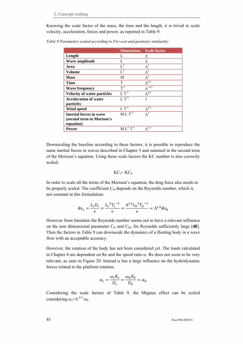
5. Concept scaling
45 Risø-PhD-80(EN)
Knowing the scale factor of the mass, the time and the length, it is trivial to scale velocity, acceleration, forces and power, as reported in Table 9.
Table 9 Parameters scaled according to Fn=cost and geometry similartity.
Dimensions Scale factor Length L Wave amplitude L Area L2
Volume L3
Mass M
Time T
Wave frequency T-1
Velocity of water particles L T-1
Acceleration of water particles
L T-2 1
Wind speed L T-1
Inertial forces in wave (second term in Morison’s equation)
M L T-2
Power M L2 T-3
Downscaling the baseline according to these factors, it is possible to reproduce the same inertial forces in waves described in Chapter 3 and summed in the second term of the Morison’s equation. Using these scale factors the KC number is also correctly scaled:
KCs= KCb
In order to scale all the terms of the Morison’s equation, the drag force also needs to be properly scaled. The coefficient CD depends on the Reynolds number, which is not constant in this formulation:
Λ .
νΛ .
However from literature the Reynolds number seems not to have a relevant influence on the non dimensional parameter CD and CM, for Reynolds sufficiently large [48]. Then the factors in Table 9 can downscale the dynamics of a floating body in a wave flow with an acceptable accuracy.
However, the rotation of the body has not been considered yet. The loads calculated
in Chapter 4 are dependent on Re and the speed ratio . Re does not seem to be very
relevant, as seen in Figure 20. Instead has a large influence on the hydrodynamic forces related to the platform rotation.
Considering the scale factors of Table 9, the Magnus effect can be scaled
considering s=-0.5b.
5. Concept scaling
46 Risø-PhD-80(EN)
Using the same scale factors, it is possible to scale also the forces of the wind on the
structure: v0s=v0b 0.5.
So far, I showed that it is possible to scale properly all the dynamics of a floating body, i.e. the platform of a floating turbine. In order to scale the whole system, it is still necessary to scale the aerodynamic forces on the rotor. The tip speed ratio,
, remains constant with the scale factors defined above, allowing a proper
scale of the rotor properties.
However when applied to reality this scaling approach has some limitations:
- This method can be applied only for test in controlled conditions. It is impossible otherwise to find a location which would fulfil all the required scale factors on wind, waves and current characteristics.
- The variation of the wind speed can be very large and eventually unrealistic in dimensioning a small model turbine. Therefore, in order to have a working small model, the wind speed and the rotational speed of the model wind turbine need to be adjusted.
- Changing the rotational speed would affect the proper scaling of the Magnus effect. Therefore, the flow stream velocity would also need a proper
adjustment to keep =cost.
This is a good method to study the physics of a full scale machine in a downscaled
model, but it is not an option to scale a concept design.
5.3 Feasibility approach: concept scaling The methodology described above can be useful to study the dynamics of a system with a scaled model and it can give a rough estimation of the full scale design in a new size. However it cannot be used to vary properly the design of a concept. A method with this purpose has to be capable to consider an efficiency factor rather than a length scale. To scale a VAWT rotor, a similarity approach can be used, assuming the efficiency of the rotor not varying in a limited range of Reynolds numbers. Than the maximum Cp of the rotor can be considered constant for a
constant tip speed ratio =R/v0.
If we consider the following equation for the power of the rotor:
0.5ρv A CP 0.5ρSCPω R
λ
And assuming the swept area of the rotor proportional to R2,
·
Then the power at a fixed tip speed ratio is equal to:
Cost · ω R

5. Concept scaling
47 Risø-PhD-80(EN)
This relationship allows scaling the power of the rotor according to the radius and
the rotational speed, for a fixed . Other similar formula can be used with the some purpose.
In design scaling, local effects of particular external conditions have to be considered. Examples are the effects of the Reynolds number on the design of small rotors which I will describe later in Chapter 9 and of the gravity in dimensioning blades for large sizes, as it will be discussed in Chapter 8.
The dimension of the platform is depending largely from the site and the location is not necessary scaled as the size. Therefore an appropriate design has to be achieved independently from any scale law.
5.4 Economical and production approach: evaluation of concept upscaling
This approach brings up new issues, such as the choice of the materials and of the manufacture process. Up -scaling studies on HAWTs are present in literature [65] and [66], and also old studies on VAWTs exist [67]. The goal of those studies is to guess the curve of the cost and mass of the components and eventually of the whole wind turbine, based on the technological learning curve and on the selection of a design with the best upscaling potential. I will discuss how this approach can be used to DeepWind in the Chapter 10.

6. Numerical code to investigate the concept
48 Risø-PhD-80(EN)
6 Numerical code to investigate the concept 6.1 HAWC2
6.1.1 Structural formulation For the numerical evaluation of the design, I use HAWC2, an aero-hydro-servo-elastic code developed by Risø DTU. The code is capable to simulate the structural response of a pitch controlled HAWT subject to aerodynamic and hydrodynamic loads, as in [30] and [33]. The core program has a multibody formulation, which in principle gives the possibility to describe any arbitrary geometry, including a VAWT.
The structure of the turbine is described as composed by several bodies, each one with an own reference system. The structural response of each body is implemented with finite element method (FEM), using Timoshenko beam formulation and assuming small deflections within the bodies. The bodies are coupled with algebraic constraints, which allow large rotations and traslations. The use of algebraic constraints automatically adds the internal reaction forces and moments on the connected elements. Different constraints are possible, such as fixed relative position, bearings and cardanic joints. More details about code capabilities are described in [38]. Figure 22 represents the multibody formulation in a glance.
Figure 22 Sketch describing the multibody formulations and the links between the individual bodies, from [38].
The aerodynamic module for a HAWT is implemented with a BEM code but it is not used in this context.
6.1.2 Hydrodynamic module The hydrodynamic module is part of the core program. The external conditions are implemented, including:
- Regular or irregular waves, according to the linear theory. The JONSWAP spectrum formulation is used for irregular waves, allowing directional spreading. Wheeler profile stretching is used for shallow waters.
- Unidirectional currents can be added. The direction is kept constant with the water depth, while there are a few possibilities to model the water shear profile. In my calculation I use a power law formulation, as I will describe later.

6. Numerical code to investigate the concept
49 Risø-PhD-80(EN)
The hydrodynamic wave-induced loads are computed using the Morison’s formulation and assuming slender bodies. The coefficients CD and CM need to be specified in the main input file for a finite number of sections of the platform.
The axial damping contributions are added at the end of the nodes, while the dynamic pressure is considered as a concentrated force and it is applied at the ends of the nodes and also distributed on conical shaped surfaces.
The hydrostatic loads are considered as concentrated forces and moments due to static pressure distributions and are distributed on the bodies.
6.2 Added DLLs HAWC2 allows the use of DLLs (Dynamic Link Library) to transfer arrays of data and to apply external forces on specific elements.
I have added some DLLs to make the code capable of investigating the DeepWind concept.
This approach allows some flexibility in adapting and testing the added sub-routines. However there are also some relevant restrictions, such as a large quantity of data to transfer, a larger input file to adapt at each new geometry and longer computation time. A further implementation of some of these DLLs in the main program will make computation more robust and faster.
6.2.1 VAWT aerodynamics I implemented the aerodynamic loads on the rotor with a BEM code for VAWTs connected to the main program with a DLL link.
The DLL routine takes input data from the main program: the position of the blade and the values of the wind velocity along the rotor height. Then the value of the wind velocity on each blade element is extrapolated.
The output array consists of the aerodynamic loads to apply on each element in the local coordinate system.
Other two external input files contain the geometrical data of the blade elements of the rotor and the aerodynamic coefficients of the airfoils for a given number of Re. It is possible to specify the values of the aerodynamic coefficients in the hysteresis loop, if such data are available.
The DLL routine has a double disk multistream tube (DDMST) formulation, based on the multistream tube model from Strickland [36] and with the double disk modification from Paravischivoiu [20]. The code follows the implementation of the induction calculation in Paulsen [68] at Risø DTU.
The first formulation of the stream tube theory used a single actuator disk and a single stream tube, see Figure 23.

6. Numerical code to investigate the concept
50 Risø-PhD-80(EN)
Figure 23Sketch describing the stream tube theory, from [69].
Strickland improved the model, dividing the rotor in several stream tubes [70]. A further modification from Paravischivoiu consists of using two actuator disks in tandem instead of the single disk used by Strickland [20]. Watching the rotor from the top, the two actuator disks divide the rotor area in two parts, one upstream and another one downstream. Each of the two actuator disks describes a surface of discontinuity and in the output of the first actuator disk is the input velocity for the second one. Figure 24 clarify the physical idea of the model, compared to previous versions. Coupled with the theory of the blade element, this formulation forms a system of independent equations equal to the number of variables.
Figure 24 Sketch describing single stream tube theory (left), multi stream tubes theory (centre) and double disk theory (right)
I do not mention here the details on the derivation of the equations, broadly described in [20], but I briefly describe the way the routine is implemented:
- First the relative velocities and angle of attacks are calculated at the azimuthal (orbital) positions of the each element, by vector summation of the wind speed and the relative velocity of the blade element.
- A stream tube with two actuator disks is considered for each element of each blade.
- The induced velocity in the upstream part of the rotor is calculated and it is used to calculate the input velocity in the downstream part of the tube.
- The values of the aerodynamic coefficients, at the local values of Re and angle of attack, are interpolated.
Stream tube theory: The free stream flow has pressure p0 and velocity U. When the flow approaches the rotor it expands. The actuator disk is included in the tube and it is a surface of discontinuity for the pressure, which pass from the value p1 to p2. A wake is generated behind the rotor but considering a control surface at a sufficiently large distance from the rotor, the pressure returns to the free stream value p0. The flow velocity is instead decreased to the value Ue=U(1-a), where a is defined as the induction generated by the rotor. The loss of moment in the flow is equal to the force generated by the flow on the rotor.

6. Numerical code to investigate the concept
51 Risø-PhD-80(EN)
- The total force on the tube is calculated and there is an iteration process to calculate the final values of the induction.
- The tangential and normal forces on the elements are computed and written in output.
Some additional features included in the DLL are:
- For angles of attack larger than the angle of static stall of the profiles, the hysteresis data of the airfoils can be used, if specified in the input.
- The data are interpolated on the Reynolds number to take the variability of the local Reynolds number with the azimuthal angle into account.
One of the most common issues in VAWT code development is the reliability of the airfoils data. I mostly used NACA 0018 profiles and I used different sources to collect airfoils data, depending of the Reynolds number range:
- Risø experimental data on a NACA0018, Paulsen [68]. The data from wind tunnel experiments include hysteresis loop values. The range of Reynolds number is between 5.3 104 and 3.96 105.
- Sandia data [71], from wind tunnel test on NACA0012 and NACA 0015 at limited range of Re. The data are extended to 104<Re<107 and to other symmetric NACA airfoils (0018, 0021, 0025), with the use of an airfoil section characteristics synthesizer computer code.
- TU Trento experimental and interpolated data for NACA 0018 and 0015 in the range 4.14 104<Re<2.97 106.
- Tu Delft data [72], from wind tunnel experiments on NACA 0018 and a cambered airfoil with 20% thickness, i.e. DU 06-W-200. The data are included in the range 3 105<Re<106.
6.3 Forces on the rotating platform In this DLL routine I compute the loads on the structure discussed in Chapter 4.
The loads are expressed as functions of non dimensional coefficients, as in Eq.9. As for the aerodynamic coefficients, the hydrodynamic coefficients are tabled in an input file.
The geometry of the platform is given in an input file. From the main program I transfer the water stream velocity at different water depths and the relative speed of each element of the platform.
The water velocity on each element is calculated by interpolation. Adding the relative motion of the tower, I obtain the velocity of the water on the surface of each element.
The lateral force, the in-line force and the friction moment on each element are calculated with the hydrodynamic coefficients from the input tables and transferred in output.
Also for this DLL, the greatest limitation is on the tabled coefficients. Unfortunately, I have, so far, only few data. For small Re ( ~10 ), values consistent with the demonstrator 1kW turbine, I use the data from the literature, [57].

6. Numerical code to investigate the concept
52 Risø-PhD-80(EN)
For the MW sizes (Re>106), there are no data in the literature and I have only very few data from CFD calculations. In this case I disregard the influence of the
Reynolds variation and I consider the variation of the coefficients linear with , for
<3.
The effect of coupling the hydrodynamic lateral force FL with the aerodynamic loads is showed in Figure 25. Two simulations were run on a floating 2 bladed VAWT (configuration 1 in section 2.6.1), in still water and the results show the motion of
the cross section of the platform at the mean water level and the tilt angle is the inclination of the platform with respect to the inertial horizontal plane, measured at the bottom cardanic connection. In my simulations in the next chapters, I use this angle to define the inclination of the platform, rather than the pitch angle or the roll angle. The wind is in the y direction and it is increased linearly from 5m/s to 25m/s.
Figure 25Effect of the Hydrodynamic force FL, from top left in clockwise order: dx (transverse to wind direction), dy (in wind direction) and the tilt angle for a VAWT running in still water at wind speed 5<v0<25m/s.
In one simulation (red line) the hydrodnamic DLL is disconnected, in the second (blue line) the DLL is connected to the aerodynamic code. The motion of the platform generates a relative velocity between the platform and the still water. Therefore additional hydrodynamic forces act on the platform. At the start the forces are negligible because of the low rotational speed. After 1000 time steps, the turbine rotates fast enough to generate a force on the x axis, caused by the motion on the y axis driven by the aerodynamic thrust. In general the hydrodynamic lateral force generates another strong coupling between the two motions on the x axis and y axis (pitch/roll, surge/sway), already linked by the gyroscopic effects. From Figure 25 more specific observations can be made about the effects of the lateral force on the dynamics:
-1.1
-0.6
-0.1
0.4
0.9
0 2000 4000 6000 8000 10000
Dx
[m]
Time steps
With FlWithout Fl
0.0
2.0
4.0
6.0
8.0
10.0
0 2000 4000 6000 8000 10000
Dy
[m]
Time steps
With Fl
Without Fl
-6.0
-5.0
-4.0
-3.0
-2.0
-1.0
0.0
0 1000 2000 3000 4000 5000 6000 7000 8000 9000 10000
Tilt
ang
le [D
eg]
Time steps
With FlWithout Fl

6. Numerical code to investigate the concept
53 Risø-PhD-80(EN)
- The main period of the motion oscillations shrinks, for both the translational motions of the tower section and the tilt angle.
- The amplitude of the oscillations of the tilt angle is slightly reduced and these variations are due to damping by the effect of the hydrodynamic forces.
- The further coupling of the motions of pitch and roll creates another variation over time, which is visible in the chart of dx, where the amplitude of the oscillations is varying during the time.
6.3.1 Generator module
The generator DLL simulates a slip induction generator, based on [73]. A slip model is included, as well as a soft starter. In order to smooth the power output (considering the strong torque ripple of Darrieus turbines), a first order low pass filter is applied on the power output. It is possible to consider the losses in the generator at different values of slip.
All the input data are written in the main input and the output array includes the produced electrical power and the torque on the shaft. Eventually the generator works also as a motor to start the turbine until reaching a rotational speed fixed in input.
6.3.2 Generator control The turbine can be controlled by regulating the rotational speed of the variable speed generator. I implemented a control based on Sandia’s experience on the control of the 17m VAWT [17].
Four rotational speeds and four wind speeds can be specified through the input array.
The control varies the rotational speed according to the wind speed v0 and to the input variables.
Since the system has a very large inertia, I considered a limit value for the acceleration of the rotor. Mostly I used a maximum acceleration of 0.1rad/s2. When the acceleration is not enough to reach the expected rotational speed, the control is delayed and the turbine runs to a lower rotational speed.
6.4 Fixed setup There are some values, hypothesises and assumptions which are essential to evaluate the results of the next chapters. Some of these values are common to all the simulations and I report them in this paragraph.
6.4.1 Physical properties The physical properties of the fluid are kept constant. The values I considered are shown in Table 10.

6. Numerical code to investigate the concept
54 Risø-PhD-80(EN)
Table 10 Characteristic of the fluids
Fluid Kinematic Viscosity Density [m2/s] [kg/m3] Air 1.51 10-5 1.21 Water 1.31 10-6 1025
During the design and the simulations, I used different materials to describe the components. Their characteristics are listed in Table 11. The properties of aluminium and steel are the most common used in engineering design, in particular for the steel I use the same value used in the Dutch DOWEC project [74]. To describe the properties of the fiberglass in pultrusion, I refer to the values pointed by Migliore and Chaney in their study of feasibility on pultruded blades for HAWTs [46].
Table 11 Properties of the materials used during the simulations
Material Young Module (E) G Density [Mpa] [Mpa] [kg/m3] Steel 2.1 1011 8.1 1010 7850 Aluminium 7.0 1010 2.8 1010 2700 Fiber glass 2.07 1010 7.59 109 1800
6.4.2 Description of external conditions Wind
The wind direction is always along the y axis. The vertical wind shear along the z axis is described by the power law:
, Eq.7
v0: reference wind speed at the equator elevation
z: local elevation from mean water level
z0: the reference elevation at the half of the rotor height.
: power coefficient set to 0.14, as from offshore standard, [49].
The wind speed shear generated in the code is not related to the computed water currents and waves. Tubulence effects are not considered.
Currents
Water currents are computed with the water shear profile described by the equation:
, Eq.8
Where:
z: local water depth
U(z): water speed at local water depth
6. Numerical code to investigate the concept
55 Risø-PhD-80(EN)
U0(t): water speed at the mean water surface
h: water depth
power coefficient set to 0.5.
The direction of the currents is defined in input from the angle c, formed by the currents with the wind direction. c is positive for currents coming from the right when looking in the wnd direction at default conditions.
Waves
Regular waves are modelled for given a, TP and water depth in input. Irregular
waves are computed using the JONSWAP spectrum, with the shape parameter equal to 3.3.
The direction of the waves is described by the angle w, which is defined positive
with the same conventions used for c.
6.4.3 Model set up The numerical results included in the next chapters regard the first configuration of the concept (Figure 10), sea bed configuration. To model the floating VAWT I used different bodies:
- A cylindrical tapered tower - 2 blades with a relative angle of 180 degrees - A generator box - A base.
The base is fixed to the sea bed in all the 6 DOF. This element is necessary because it is not possible to anchor the generator at the sea bed with a cardanic joint.
The generator box is instead connected to the base with a cardanic joint, fixing the three translational DOF and the yaw, around the z axis. Then the generator can rotate, with respect to the basement, back and forth and to the sides (pitch and roll).
The tower is fixed to the generator box with a bearing that allows only one rotational degree of freedom, i.e. the yaw around the vertical axis, z.
The blades are fixed to the tower in all the 6 DOF.
6.4.4 Reference systems The model of the turbine is shown in Figure 26 along with the used reference systems. The base reference system is solidal to the inertial reference system and I neglected in the sketch.
The properties of each coordinate system respect to the inertial one are given in Table 12.

6. Numerical code to investigate the concept
56 Risø-PhD-80(EN)
Figure 26 Reference systems used to describe the floating VAWT.
Table 12 Reference system description
Reference system Properties Global reference system XG, YG, ZG (g.r.s.)
Inertial reference system XG, YG lay on the mean water plane ZG directed towards the seabed
Generator box reference system Xgb, Ygb, Zgb (gb.r.s.)
The origin is on the first node of the gear box body
At t=0 the three axis are parallel to axis of the g.r.s.
During the simulation the system is free to rotate around Xgb and Ygb
Tower reference system XT, YT,ZT (t.r.s.)
The origin is on the first node of the tower body
ZT rotates around Zgb at r XT and YT are parallel and solidal to
Xgb and Ygb Blade reference system XB, YB,ZB (b.r.s.)
The origin is on the first node of the blade body
XB, YB and ZB are solidal and parallel to XT, YT and ZT
Local reference system XL, YL,ZL (l.r.s)
The origin is on the first node of the element
ZL is tangential to the blade centerline
XL lays in the plane formed by the two blades; it is perpendicular to the blade centreline and it is directed towards the tower.
YL is parallel to YB. Wind speed reference system Xw, Yw,Zw (w.r.s.)
Xw, Yw and Zw are solidal and parallel to XT, YT and ZT

6. Numerical code to investigate the concept
57 Risø-PhD-80(EN)
The direction of the wave propagation and of the water stream flow (marine currents) will be referenced to the inertial coordinate system and will always be in the horizontal plane, i.e. the currents have no vertical component.
6.5 Calculation points During numerical simulations even though I change the design and the dimensions, I record the results at the same points on the turbine. These points are plotted in Figure 27 and described in the next table.
Figure 27 Position of the measurements points on the floating VAWT, dimensions are not
indicative of the real design.
6.6 Other software used for numerical simulations Other programs have been used in the current work for some dedicated tasks.
- The CFD software EllipSys2D from Risø DTU, to calculate the force and moment coefficient in currents.
- Some other routines or calculations have been implemented using other software: Matlab, Compaq Visual Fortran, Excel, Sigma plot.
Points N.
Body Position on the body
1 Tower top 2 Blade centre root 3 Blade lower root 4 Tower blades connection 5 Tower mean water level 6 Tower bottom 7 Generator
box bottom

7. First iteration design: 2MW
58 Risø-PhD-80(EN)
7 First design: 2MW The 2MW turbine was the first attempt to design a DeepWind concept turbine for numerical simulation and evaluation. Previously, studies had been conducted on 3 sizes (1MW, 5MW, 20MW) without fully integrating the design of the rotor with the design of the platform [75].
One reason to select a 2MW design was to have a size comparable with the Hywind concept, which was designed for 2.3MW. However the 2MW design was mostly used as a first base design to develop the code and to investigate the effects of the hydrodynamic forces on the rotating platform.
Before describing the study on the 2MW, I would like to make a few clarifications:
- The design had several changes during the time. To facilitate the understanding to the reader I have selected only the results analysis coming from one design.
- Some components and some aspects of the design have not been fully described in detail, mainly due to the purpose of the study.
- The 2MW has been used for the investigation of the Magnus effect on the rotating platform. This has eventually resulted in higher hydrodynamic loads than expected and the design is not fully tailored for those hydrodynamics forces and moments.
- The code has been developed in parallel to the design, therefore the study on the 2MW has been carried out with a preliminary and simplified version of the DLL and of the coupling with HAWC2.
7.1 Design specifications
7.1.1 Rotor design The solidity of the rotor (=Nc/R), is equal to 0.19. This value is a compromise
between the optimization of the rotor performances (higher values of ) and the
reduction of the cost (0.1 is the optimum value), [20].
The aspect ratio of the rotor, defined as ratio between height and diameter, is 1.12. Also this value is a compromise between the optimum, discussed by Paraschivoiu to be around 1.3 [20], and the reduction of the costs, obtained by reducing the height. It is useful to stress that a taller rotor in turn also requires a deeper foundation. This means higher costs in terms of: longer structure, larger forces on the submerged part and larger values of the frictional losses to the nominal power. The properties of the rotor are included in Table 13.
The turbine has a cut-in wind speed of 5 m/s, a cut-out wind speed of 25 m/s and the rated power is achieved at 14m/s, consistent with offshore environment and high
wind resources. The rotational speed is regulated in order to work at the of maximum efficiency, i.e. considering the solidity and the Reynolds number of the
rotor, =5.2. is kept equal to 5.2 untill the maximum rotational speed is reached,
i.e. 14rpm. Then the rotational speed remains constant and decreases. Meanwhile,

7. First iteration design: 2MW
59 Risø-PhD-80(EN)
the power increases until reaching the rated power of 2.35MW at 14m/s. From this condition the power is kept constant, reducing the rotational speed, untill a wind speed of 17.25m/s and a rotational speed of 12.5rpm. For wind speed higher than 17.25m/s, the rotational speed is kept constant and the power is reduced until 1.63MW at 25m/s, when the turbine is stopped. The power and the corresponding rotational speeds are shown in Figure 28.
This control is different from the power curve showed in Figure 16 of chapter 4. In that case the power was kept constant while increasing the rotational speed. As discussed before, that would be a less robust control because a reduction in the wind speed can cause an increase of the power. Therefore in the study included in this chapter, I have decided to control the rotor by reducing the rotational speed as explained above.
Figure 28 Power curve and rotational speed of the rotor.
The design process has followed the process described in section 1.4, although it has not been tailored to take into account very high loads due to the currents. The platform is tapered to reduce the wave-induced loads near the surface and the dimensions are reported in Table 13.
Table 13 Main design parameters of the 2MW turbine.
0
2
4
6
8
10
12
14
16
0.0E+00
5.0E+05
1.0E+06
1.5E+06
2.0E+06
2.5E+06
0 2.5 5 7.5 10 12.5 15 17.5 20 22.5 25 27.5
rota
tion
al s
peed
[rp
m]
Pow
er [
W]
Wind speed [m/s]
Power Rotational speed
2MW Specifications Rotor Diameter [m] 67
Rotor Height [m] 75
Chord of the blade [m] 3.2
Torque at rated power [Nm] 1.4 106 Thrust at rated power [N] 2.4 105 Rotational speed at rated power
[rpm] 15.0
Diameter of the tower above the water level
[m] 4.0
Maximum diameter of the platform (Tapered tower)
[m] 7
Total water displacements [m3] 3000
Total length [m] 183

7. First iteration design: 2MW
60 Risø-PhD-80(EN)
The design and the simulations investigate the 1st configuration (sea bed configuration) described in 2.6.1 with the bottom of the platform fixed at the sea bed and without translational degrees of freedom.
7.2 Load cases and code set up The 2MW VAWT was not tested referring to a specif site. Instead I selected some conditions to investigate the behaviour of the turbine and to verify the code was working properly.
Here, I present the results from four simulations, corresponding to different combinations of wind, waves and currents, as summarized in Table 14. In each load case, the turbine is started up by the generator. At the time of these simulations, there were some limitations in the code:
- The aerodynamic loads are integrated on each blade and they are applied directly on the tower (i.e. no aerdynamical loads are applied on the blade elements)
- The relative speed of the platform is not considered in the calculations of the hydrodynamic lateral force Fl.
The simulations were run at constant wind speed, therefore the control showed in Figure 28 is not implemented. Instead when the rotational speed reaches the rated level of 15rpm, it is kept constant by the generator.
A summary of the load case is shown in Table 14.
Table 14 Load cases summary
Wind Waves CurrentsLoad case 0 X 1st load case X X 2nd load case X X 3rd load case X X X
7.2.1 Wind speed The vertical variation of the wind speed v0 along the z axis is described by the power law in equation Eq.7 of Chapter 6.4.2. The used values are
v0: 14m/s, it is constant over the time.
z0: 52.5m.
: 0.14 as for offshore standard, [49].
7.2.2 Currents Water currents are computed, whit a direction (x axis) transversal to the wind (y
axis), i.e. c=90deg

7. First iteration design: 2MW
61 Risø-PhD-80(EN)
The water velocity is constant, 1.0m/s at the water surface and zero at the sea bottom. The water shear profile is described by equation Eq.8 in paragraph 6.4.2 (see Figure 29). I used the following values:
U0(t)=cost= 1m/s
0.5
Figure 29 Water shear profile
7.2.3 Waves The angle w between the wind and the waves is set equal to 90deg. Thus, regular waves are modeled on the x direction. The significant wave height is 4.0m and the wave period is 9.0s. The moderate intensity of the sea state is justified with the intention to test the effect of the hydrodynamic currents loads. Figure 30 shows plot of the velocity of waves at the surface level, icluding the height of the waves.
Figure 30 z coordinate of the water surface plane (left ) and oscillatory flow at the water surface (right) for the wave condition used.
7.3 Results The load cases are investigated in the time domain and in the frequency domain using an FFT transformation. In all the four cases the turbine was started from a
condition of =0 and =0, with and respectively the rotational speed and the tilt angle of the floating turbine.
The results of the computations for the four load cases are presented in two sections: time domain and frequency domain. The parameters considered in the investigations are:

7. First iteration design: 2MW
62 Risø-PhD-80(EN)
- Displacement dx and dy of the tower cross section at the mean water surface level, point 5 in Figure 27.
- Force Fx and Fy measured on the tower at the bottom of the blades (15m above the water surface level), point 4 in Figure 27.
- Bending moment Mx and My measured at the water surface cross section of the tower, point 5 in Figure 27.
- Vertical force Fz measured at the bottom of the tower, point 6 in Figure 27.
All the variables are calculated in the global reference system of Figure 26.
7.3.1 Load case 0 The turbine is tested in still water to observe the dynamic response of the turbine in absence of hydrodynamic external loads. The aerodynamic loads are present and have a large variability, as shown in Figure 31. The time series is divided into starting conditions (30s-60s) and rated conditions (300s-350s). As neither waves nor rotational speed are present, the forces are equal to zero at the starting of the turbine. At the rated conditions the forces consist of the harmonic aerodynamic side force Fx, with a null mean value; and the aerodynamic harmonic thrust force Fy with mean value of 2.39 105N.
The displacements dx and dy of the platform at the mean surface level are plotted in Figure 32. The maximum value of the tilt angle is 1.5 degrees and it is recorded at the start of the rotor.
Figure 31 Fx, Fy on the tower section 15m above the sea (Point 4 in Figure 27). First time series (30-60s) with no rotation of the rotor, second time series (300-350s) at rated conditions.

7. First iteration design: 2MW
63 Risø-PhD-80(EN)
Figure 32 Displacements dx and dy (in meters) of the platform at the mean surface level, load case 0
7.3.2 Load case 1 Time domain
In load case 1 the currents are added to the input file and the water velocity is described by the shear profile of Figure 29. The water current direction lays on the x positive direction and the hydrodynamic side force acts on the y axis (positive direction). The aerodynamic loads are the same as in Figure 31.
The response of the turbine to the hydrodynamic and aerodynamic loads is show in Figure 33 in terms of displacements dx and dy. The turbine experiences first a peak at the start of the rotor and a more pronaunced peak at the maximum rotational speed at 15rpm. The corresponding maximum value of the tilt angle is 13.7 degrees. However the motion is damped as the turbine is in equilibrium with the external
loads at an tilt angle .

7. First iteration design: 2MW
64 Risø-PhD-80(EN)
Figure 33 Displacements dx (top) and dy (middle) in meters of the platform at the mean surface level and rotational speed (bottom) - Load case 1
Frequency domain
The power spectral density (PSD) is computed for the most relevant variables recorded on the output. In Figure 34, dx reaches a peak at the f2p frequency (0.5Hz), where f2p is the even rotational freqeuency of the rotor as defined in 3.2. The same it is visible in Figure 35 for the PSD of Fz. The two components of the bending moment reach the peak at the odd rotor rotational frequencies (f1p and f3p), see Figure 36. Finally in Figure 37, the PSD of the component Fx and Fy is shown. The f2p frequency and the higher harmonics are visible.
Figure 34 Density power spectrum of the displacement dx, dy
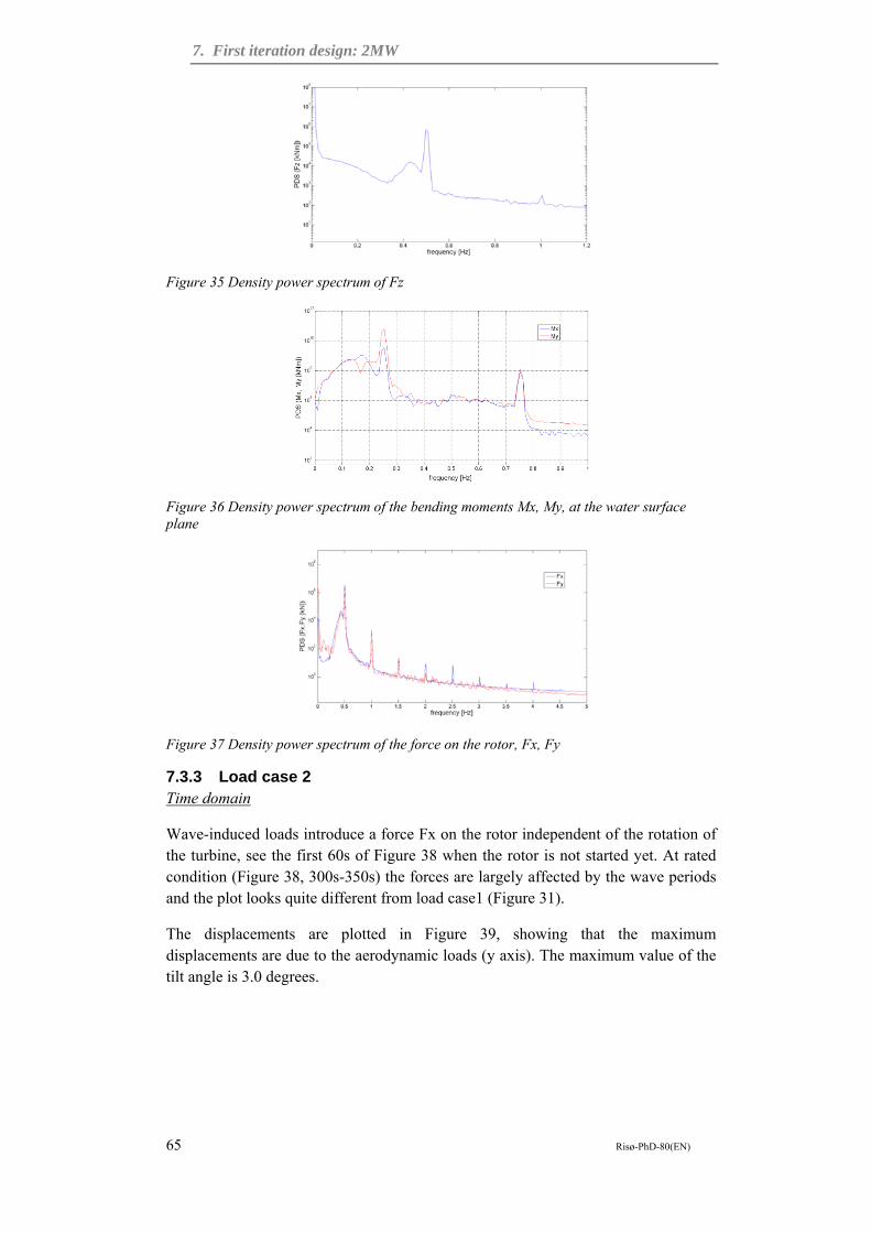
7. First iteration design: 2MW
65 Risø-PhD-80(EN)
Figure 35 Density power spectrum of Fz
Figure 36 Density power spectrum of the bending moments Mx, My, at the water surface plane
Figure 37 Density power spectrum of the force on the rotor, Fx, Fy
7.3.3 Load case 2 Time domain
Wave-induced loads introduce a force Fx on the rotor independent of the rotation of the turbine, see the first 60s of Figure 38 when the rotor is not started yet. At rated condition (Figure 38, 300s-350s) the forces are largely affected by the wave periods and the plot looks quite different from load case1 (Figure 31).
The displacements are plotted in Figure 39, showing that the maximum displacements are due to the aerodynamic loads (y axis). The maximum value of the tilt angle is 3.0 degrees.

7. First iteration design: 2MW
66 Risø-PhD-80(EN)
Figure 38 Fx, Fy on the tower section 15m above the sea. First time series (20-60s) with no rotation of the rotor, second time series (300-350s) at rated conditions.
Figure 39 Displacements dx (top) and dy (bottom) of the platform at the mean surface level - Load case 2
Frequency domain
The waves effect on the displacements of the turbine is visible in Figure 40, where a peak at the wave frequency (0.11Hz) is noticeble. The same peak is achieved for the forces Fz (Figure 42) and Fx (Figure 41). However Fy still shows a stronger dependency of the rotational frequencies, see Figure 41.
Figure 40 Density power spectrum of the displacement dx, dy

7. First iteration design: 2MW
67 Risø-PhD-80(EN)
Figure 41 Density power spectrum of the force on the rotor, Fx, Fy
Figure 42 Density power spectrum of the vertical force Fz
7.3.4 Load case 3 Time domain
The forces acting on the tower above the sea surface with all combined loads do not show significant changes from the forces where only wave loads are added, i.e. Figure 38. Furthemore, hydrodynamic loads are added because of the currents. The displacements are larger than in the previous cases, see Figure 43. The maximum angle of tilt is 13.8 degrees, which is very close to the 1st load case.
Figure 43 Displacements dx (top) and dy (bottom) of the platform at the mean surface level - Load case 3

7. First iteration design: 2MW
68 Risø-PhD-80(EN)
Frequency domain
As the currents are included in the computation of this load case, the wave frequency becomes dominant also in the displacement along the y direction, see Figure 44. Meanwhile, due to the large displacements, the dominant frequency of Fz (Figure 45) is f2p as in the first load case (Figure 35). Both the rotational and the waves frequencies are noticeable for Fx and Fy, in Figure 46.
Figure 44 Density power spectrum of the displacements dx, dy
Figure 45 Density power spectrum of the vertical force on the rotor, Fz
Figure 46 Density power spectrum of the force on the rotor, Fx, Fy
7.4 Discussion The results show a strong coupling between the pitch and the roll motions of the platform. This is partially due to the fact that the turbine acts as a gyro during its

7. First iteration design: 2MW
69 Risø-PhD-80(EN)
motion. This means that when the tower is turning, a moment applied on the x axis causes a reaction moment in the y axis.
The coupling of the two motions is also generated by the nature of the hydrodynamic side force, acting on the direction transverse to the currents direction. Thus a variation of the waves intensity in the x direction will affect also the equilibrium along the y direction, as seen by comparing Figure 34 and Figure 44.
Another strong coupling exists between aerodynamic and hydrodynamic loads. Indeed in wave-induced motion, the dominant period of the aerodynamic forces corresponds to the wave frequency. At the same time, also hydrodynamic forces and the friction moment are strongly dependent on the rotational speed of the rotor.
However, the hydrodynamic loads seem to be dominant on the dynamics of the system. Indeed the turbine operates with a tilt angle strongly dependent on the water currents speed. Once the turbine achieves the equilibrium, the tower experiences an elliptical motion on the water surface plane. The amplitude of the elliptical motion seems to be strongly dependent on the amplitude of the waves.

8. Baseline model: 5MW
70 Risø-PhD-80(EN)
8 Baseline model: 5MW I selected a 5WM size as the baseline model to evaluate the concept. The main reasons to motivate this choice were:
- Offshore wind energy is developing towards larger wind turbines and 5MW is a reasonable target at the present time.
- Looking at an evaluation of the DeepWind concept versus other floating concepts, most of them use as rotor the 5MW horizontal axis rotor from MIT/NREL [43]. This choice is intended to facilitate a future comparative study.
- 5MW is referred to a reasonable size, at which VAWTs can compete with HAWTs, thank to better upscaling potential, [22].
8.1 Design specifications The design follows the iterative process of Figure 5 and takes into accounts the dependencies addressed in Figure 4. However, to help the comprehension, here the design will be presented following a straight consequential line without any feedback in the process.
There are not specific public standards for classification of floating offshore VAWTs. Then I refer to different guidelines: the IEC standard for offshore wind turbines [49], even though it is mainly focused on HAWTs and fixed bottom foundations; the standard from the French Bureau [76] is probably the most relevant one, being specifically meant for floating wind turbines; the standard from DNV [77], which is mainly thought for O&G industry, and is still the most complete guideline on the procedures for modelling waves and currents; the standard from NORSOK [78] addresses procedures and guidelines for offshore structure, with particular emphasis on North Sea conditions.
8.1.1 Site description All the standards mentioned above agree on the need of joint met-ocean data for a correct evaluation of an offshore design. In the current study, in addition to joint statistical data describing waves and wind conditions, there is a necessity of accurate data on the sea currents at the site. A full set of data with these requirements was not available. At a first moment, I collected data from Sletringen, a location just west of Trondheim in Norway, where Oceanor is conducting a measurement campaign. The data included wind at three elevations, wave characteristic values and sea currents at several water depths. Unfortunately some technical problems occurred at the site and at present I have not enough data for a statistical evaluation of the site conditions.
An alternative solution has been proposed from DHI in a report for the DeepWind project [79]. The selected site is the test site used by Statoil for Hywind, situated off of the Norwegian cost of Stavanger, see red dot in Figure 47. Missing statistic data, a selection of the most relevant sea states can be made referring to the standards: [78], [77].

8. Baseline model: 5MW
71 Risø-PhD-80(EN)
First, I selected the main objective of the design verification, which I decided should be the dynamics of the floating turbine in the most extreme external states for operation conditions of the turbine. I assume that the rotor has to work for wind speeds up to 25m/s.
The currents are composed from different terms, depending on the cause which generates them: tidal currents, wind driven currents, coast and ocean currents, local eddy currents, currents over steep slopes, currents caused by storm surge, internal waves. Here, I consider only the first two terms. Missing real data, the maximum value of the tidal currents is estimated from Figure 64 to be 0.2m/s. The wind-driven currents can be obtained as 2% of the hourly average wind speed at an elevation of 10m above the mean water level. Considering v0=25m/s, as the maximum operation wind speed, the maximum value of the wind driven currents is taken equal to 0.5m/s. Therefore the total current velocity at the surface is 0.7m/s. Similar values are also available in literature, as in [80] and [81]. Additionally, these papers show that moving further from the Norwegian cost, relevant underwater currents are present and the concept design would be more challenging.
Figure 47Maximum 100 year tidal surface current [m/s](left). Significant wave height Hs and related maximum peak period TP with annual probability of exceedance of 10-2 for sea-states of 3 h duration. ISO-curves for wave heights are indicated with solid lines while wave period lines are dotted, maps from [78]. The red dot represents the selected site. The 100 year significant wave height H100, can be estimated from Figure 47. Then I considered Hs=14m and TP=16s, as most critical sea state. More moderate conditions can be added for the analysis.
A list of the most critical conditions expected at the site is reported in Table 15. I disregard in my work other external factors, such as ice, snow and earthquakes.
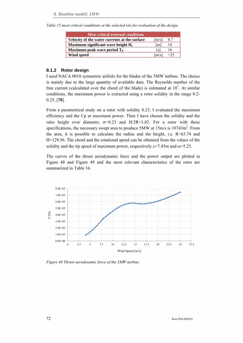
8. Baseline model: 5MW
72 Risø-PhD-80(EN)
Table 15 most critical conditions at the selected site for evaluation of the design.
Most critical external conditions Velocity of the water currents at the surface [m/s] 0.7 Maximum significant wave height Hs [m] 14 Maximum peak wave period TP [s] 16 Wind speed [m/s] <25
8.1.2 Rotor design I used NACA 0018 symmetric airfoils for the blades of the 5MW turbine. The choice is mainly due to the large quantity of available data. The Reynolds number of the free current (calculated over the chord of the blade) is estimated at 107. At similar conditions, the maximum power is extracted using a rotor solidity in the range 0.2-0.25, [70].
From a parametrical study on a rotor with solidity 0.23, I evaluated the maximum efficiency and the Cp at maximum power. Then I have chosen the solidity and the
ratio height over diameter, =0.23 and H/2R=1.02. For a rotor with these specifications, the necessary swept area to produce 5MW at 15m/s is 10743m2. From the area, it is possible to calculate the radius and the height, i.e. R=63.74 and H=129.56. The chord and the rotational speed can be obtained from the values of the
solidity and the tip speed of maximum power, respectively c=7.45m and =5.25.
The curves of the thrust aerodynamic force and the power output are plotted in Figure 48 and Figure 49 and the most relevant characteristics of the rotor are summarized in Table 16.
Figure 48 Thrust aerodynamic force of the 5MW turbine.
0.0E+00
1.0E+05
2.0E+05
3.0E+05
4.0E+05
5.0E+05
6.0E+05
7.0E+05
8.0E+05
0 2.5 5 7.5 10 12.5 15 17.5 20 22.5 25 27.5
F [
N]
Wind Speed [m/s]
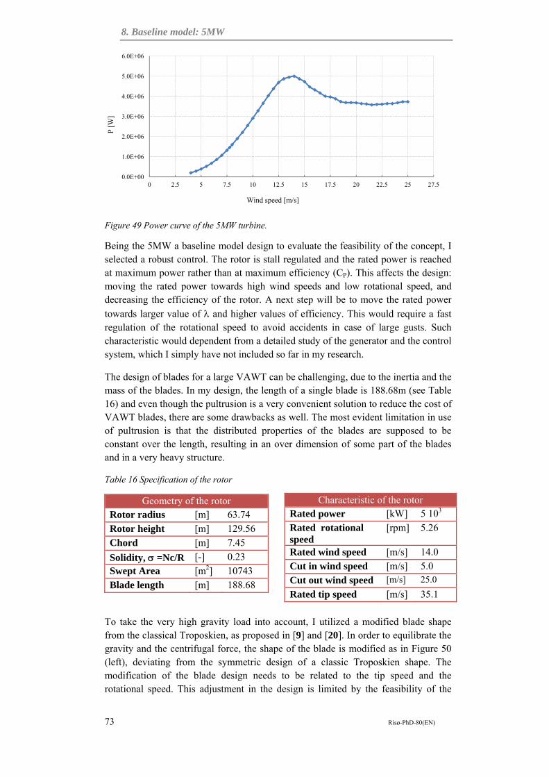
8. Baseline model: 5MW
73 Risø-PhD-80(EN)
Figure 49 Power curve of the 5MW turbine.
Being the 5MW a baseline model design to evaluate the feasibility of the concept, I selected a robust control. The rotor is stall regulated and the rated power is reached at maximum power rather than at maximum efficiency (CP). This affects the design: moving the rated power towards high wind speeds and low rotational speed, and decreasing the efficiency of the rotor. A next step will be to move the rated power
towards larger value of and higher values of efficiency. This would require a fast regulation of the rotational speed to avoid accidents in case of large gusts. Such characteristic would dependent from a detailed study of the generator and the control system, which I simply have not included so far in my research.
The design of blades for a large VAWT can be challenging, due to the inertia and the mass of the blades. In my design, the length of a single blade is 188.68m (see Table 16) and even though the pultrusion is a very convenient solution to reduce the cost of VAWT blades, there are some drawbacks as well. The most evident limitation in use of pultrusion is that the distributed properties of the blades are supposed to be constant over the length, resulting in an over dimension of some part of the blades and in a very heavy structure.
Table 16 Specification of the rotor
Geometry of the rotor Rotor radius [m] 63.74
Rotor height [m] 129.56
Chord [m] 7.45
Solidity, =Nc/R [-] 0.23
Swept Area [m2] 10743
Blade length [m] 188.68
To take the very high gravity load into account, I utilized a modified blade shape from the classical Troposkien, as proposed in [9] and [20]. In order to equilibrate the gravity and the centrifugal force, the shape of the blade is modified as in Figure 50 (left), deviating from the symmetric design of a classic Troposkien shape. The modification of the blade design needs to be related to the tip speed and the rotational speed. This adjustment in the design is limited by the feasibility of the
0.0E+00
1.0E+06
2.0E+06
3.0E+06
4.0E+06
5.0E+06
6.0E+06
0 2.5 5 7.5 10 12.5 15 17.5 20 22.5 25 27.5
P [
W]
Wind speed [m/s]
Characteristic of the rotor Rated power [kW] 5 103
Rated rotational speed
[rpm] 5.26
Rated wind speed [m/s] 14.0
Cut in wind speed [m/s] 5.0
Cut out wind speed [m/s] 25.0
Rated tip speed [m/s] 35.1

8. Baseline model: 5MW
74 Risø-PhD-80(EN)
manufacture process. I considered the design blade shape in Figure 50, which is tailored for a tip speed of 36.3m/s which is very close to the one reported in Table 16 and for 30rpm that is much higher than the rated 5.26 of my design. However, the benefit of the modified shape of the blade is visible in the right picture of Figure 50, where I have plotted two time series of the moment around the local y axis (see Figure 26) at the lower root of the blade (point 3 in Figure 27). In the modified design the load is reduced and the mean value decreases with the increase of the rotational speed, by the effect of the centrifugal force. A further modification to the design is possible and it would be recommended, in order to lower the bending moment on the blade. However, it seems to be challenging to reach the full tensional equilibrium between the gravity and the centrifugal force, with a shape of the blade which is reasonable simple to manufacture. A compromise in the design could then include a possible rise in the rated rotational speed.
Figure 50 Blade shape for a classic Troposkien and Troposkien modified for the effect of Gravity (left). Effect of the blade shape on the bending moment at the low root of the blade (right).
I used the blade structure in Figure 51 and the distributed properties in Table 17 to describe the blade sections over the length. The properties of the material are reported in Table 11. However, in order to avoid major deformations, it has been necessary to reinforce the structure of the blade close to the connection with the rotor. Then I considered stiffer and heavier structure over the two extremities of the blade over a length of 36.7m from the top and 45.5m from the bottom. The length of the central part of the blade is 107m. The final design of the blade has a weight of 1.54 105 kg, as reported in Table 17.
Figure 51 Section for the central part of the blade of the 5MW turbine. 2D sketch with dimensions (left) and 3D drawing (right), kindly provided by Per Hørlyk Nielsen from Risø DTU.
0
0.2
0.4
0.6
0.8
1
1.2
1.4
1.6
1.8
2
0 0.25 0.5 0.75 1
z/H
y/R
Troposkien modiefiedTroposkien
-1.4E+04
-1.2E+04
-1.0E+04
-8.0E+03
-6.0E+03
-4.0E+03
-2.0E+03
0.0E+00
0 1000 2000 3000 4000 5000
My
[kN
]
Samples
Troposkien modified
Troposkien

8. Baseline model: 5MW
75 Risø-PhD-80(EN)
Table 17Properties of the blade.
Undistributed properties of the bladesLength 1 blade [m] 188.68 Weight 1blade [kg] 1.54 105
Distance of the centre of gravity from water level [m] 60.78 Distance centre of gravity from the centre of the tower
[cm] 33.61
Ixx [kg m2] 8.99 108 Iyy [kg m2] 1.14 109 Izz [kg m2] 2.42 108
Table 18 Sectional properties of the blades.
Distributed properties of the blades Linear density [kg/m] 810.0
Area of the cross section [m2] 3.87 10-1
Ix [m4] 1.06 10-2 Iy [m4] 1.19 10-1 E [N/m2] 1.60 1010
To dimension the tower, I consider the simultaneous action of the bending moment and of the torsion moment caused by the reaction torque of the generator, and I have
calculated it at the mean water level. The design stress s at the external surface of the cylinder is:
Eq.9
Where Mb is the maximum value of the bending moment, RT the maximum external radius of the tower, Q the maximum value of the torque and IP the polar moment of
inertia of the section, .
A HAWT experiences only the first term of the equation above, thus a floating VAWT with a rotating foundation has an additional load on the tower. On the other hand, the bending moment applied on a HAWT tower is larger, due to the higher elevation of the application point of the aerodynamic thrust. Eventually the maximum stress on the tower has similar values in the two cases, disregarding any fatigue load. To dimension the tower, I considered a safety factor of 4 defined as
, where max is the material yield strength, as in the material properties of
section 6.4. The wanted safety factor fs can be achieved with a proper dimensioning of the external radius and thickness of the tower section. Also, the selection of the tower section is a result of a compromise between two solutions:
- A slender cylinder with thick walls, that would reduce the wave loads at the mean water level
- A large cylinder with thin walls, which would decrease the weight, optimising the cost.
I have selected a cross section of radius 3.15m and thickness 0.02m.

8. Baseline model: 5MW
76 Risø-PhD-80(EN)
Table 19 Properties of the tower of the rotor.
Geometry of the tower above sea level (rotor) Total length above sea level [m] 145 Clearance from mean water level [m] 15 External radius of the tower [m] 3.15 Thickness of the tower [m] 0.02
8.1.3 Platform design The platform consists of a tapered structure attached to the rotor tower at the main water level. At the connection point, the radius and the thickness are equal to the properties of the tower cross section mentioned above. At 5m below the sea level the cylinder is tapered to reach the maximum diameter of the platform, i.e. 8.3m. The tapered part of the platform is 10m long and the properties are varied linearly between the top section and the bottom section. The geometry of the platform is described in Table 20.
Table 20 Dimensions of the platform.
Geometry of the tower below sea level (platform)
Total length below sea level (HP)
[m] 108
Depth of the slender part (H1)
[m] 5
Radius of the slender part (RT)
[m] 3.15
Thickness of the slender part
[m] 0.02
Length of the tapered part (H2)
[m] 10
Length of the bottom part (H3)
[m] 93
Maximum radius of the platform (RP)
[m] 4.15
Thickness of the bottom part
[m] 0.05
Some ballast has to be added to the bottom to achieve the hydrostatic equilibrium of the platform. I considered the weight of the generator included in the mass of the ballast, placed at the bottom of the platform, with centre of gravity located at 4.78m from the bottom. The total mass of the cylindrical structure (tower and platform), including ballast and generator, is 5680tons with a centre of gravity located at an elevation of 27.84m from the bottom. The water displacements of the platform are 5940m3 and the centre of buoyancy is at 18.57m above the centre of gravity, as stated in Table 21.
Table 21 Undistributed properties of the tower.
Properties of the tower (rotor + platform) Total length (rotor + platform) [m] 253

8. Baseline model: 5MW
77 Risø-PhD-80(EN)
The distribution of the mass and of the volumes has been designed in order to have maximum angle of inclination around 10degrees. The coefficients of hydrodynamic restoring and of the natural periods of the platform are presented in Table 22. I used the parallel axis theorem (or Huygens-Steiner theorem), to include the rotor in the calculation of the natural period of the pitch mode. As shown in the table, the pitch natural period increases considerably due to the large inertia of the rotor. I report also the coefficient and the period of the platform in heave, even though the platform is anchored to the bottom, since the system is supposed to be easily adapted to the configuration with catenary mooring lines.
Table 22 Hydrodynamic restoring coefficients and natural periods in heave and pitch.
Platform stability properties C44=C55 [kg m2/s2] 1.08 109
C33 [kg /s2] 3.06 105 Tn3 [s] 27.59 (0.0362Hz) Tn4 [s] 25.97 (0.0385Hz) Tn4 (including rotor) [s] 33.96 (0.0294Hz) I decided to test the design for the sea states described in Table 15, and for other two more moderate sea states, described in Table 23, with maximum significant height values Hs between 4m and 14m and maximum wave peak period TP between 9s and
16s. For the three sea states I calculated the non-dimensional parameters D/w, oscillatory Reynolds number and KC number and I plotted the values over the local water depth in Figure 52, Figure 53 and Figure 54.
Table 23 Properties of the selected sea states.
Sea states Hs [m] TP [s] Sea State1 4 9 Sea State2 9 13.2 Sea State3 14 16
The values of the D/w are much smaller than 0.2 for all the sea states.From literature and standards the diffraction loads are therefore not relevant for the design, and potential theory can be used. The references are [77], [78], and [48].
9 The properies of the generator a
Weight (included ballast and Generator)9 [kg] 5.64 106
Ixx=Iyy [kg m2] 1.87 1010
Izz [kg m2] 2.12 107
Distance of centre of gravity from tower bottom [m] 27.84 Distance of centre of gravity from centre of buoyancy
[m] 18.57
Total water displacements [m3] 5.94 103
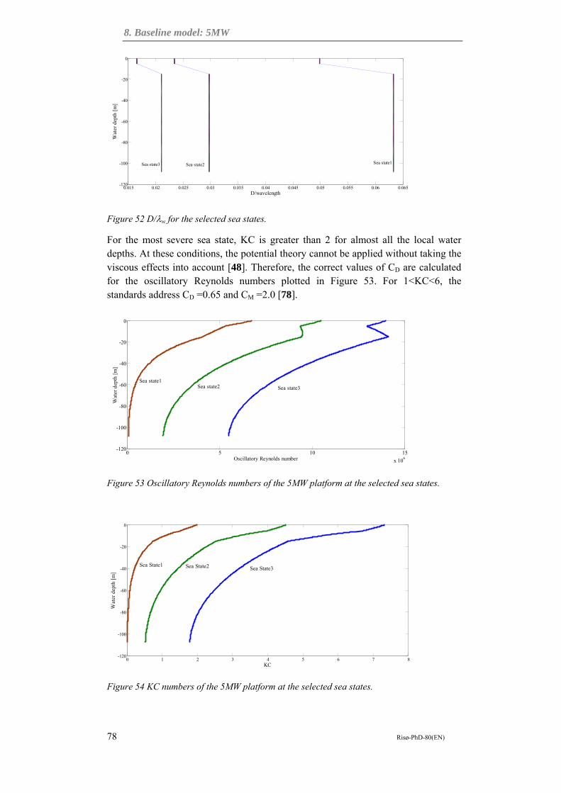
8. Baseline model: 5MW
78 Risø-PhD-80(EN)
Figure 52 D/w for the selected sea states.
For the most severe sea state, KC is greater than 2 for almost all the local water depths. At these conditions, the potential theory cannot be applied without taking the viscous effects into account [48]. Therefore, the correct values of CD are calculated for the oscillatory Reynolds numbers plotted in Figure 53. For 1<KC<6, the standards address CD =0.65 and CM =2.0 [78].
Figure 53 Oscillatory Reynolds numbers of the 5MW platform at the selected sea states.
Figure 54 KC numbers of the 5MW platform at the selected sea states.
0.015 0.02 0.025 0.03 0.035 0.04 0.045 0.05 0.055 0.06 0.065-120
-100
-80
-60
-40
-20
0
D/wavelength
Wat
er d
epth
[m
]
Sea state1Sea state3 Sea state2
0 5 10 15
x 106
-120
-100
-80
-60
-40
-20
0
Wat
er d
epth
[m
]
Oscillatory Reynolds number
Sea state1Sea state2 Sea state3
0 1 2 3 4 5 6 7 8-120
-100
-80
-60
-40
-20
0
KC
Wat
er d
epth
[m
]
Sea State1 Sea State2 Sea State3

8. Baseline model: 5MW
79 Risø-PhD-80(EN)
8.2 Simulations
8.2.1 Load cases description I carried out simulations on the configuration of the system with the generator fixed at the sea bottom described in chapter 2.6.1.
The wind velocity varies linearly in the range 5m/s<v0<25m/s. The shear profile is described from equation Eq.7 in 6.4.2 with the shear factor 0.14.
The current velocity at the surface is 0.7m/s and the water shear profile varies over z, according to equation Eq.8 in 6.4.2 with the shear factor 0.5. I considered the wave properties of the three sea states in Table 23, using both regular and irregular wave formulation. The water depth is taken equal to 110m.
The Morison’s coefficients are selected according to the considerations above with CD=0.65 and CM=2.
To handle the large number of simulations I will use a three digits number to describe each numerical time series, i.e. SimXYZ. Where X is a number describing
the sea state, Y the wave direction w and Z the current direction c, according to the numbers set in Table 24. For instance, the simulations of the sea state2 with
w=90degrees and c=45degrees is called Sim223.
Table 24 Definition of time series simulation indices
Still water Sea state1 Sea state2 Sea state3 Sea state no (TP, a)
0 1 2 3
No waves 180 Deg 90 Deg 45 Deg 0 Deg -45 Deg -90 Deg Wave direction no (w)
0 1 2 3 4 5 6
No currents 180 Deg 90 Deg 45 Deg 0 Deg -45 Deg -90 Deg
Current direction no (c)
0 1 2 3 4 5 6
8.2.2 Results First, I carried out runs in still water and without aerodynamic loads on the rotor, i.e. no wind. In Figure 55, the results from a turbine spinning in still water and started
with an tilt angle 0=10 degrees are plotted.

8. Baseline model: 5MW
80 Risø-PhD-80(EN)
Figure 55 Turbine spinning in still water, started from an inclination angle of 10degrees. Tilt angle time series (top) and PSD of the time series using logarithmic scale (bottom). Note for the top figure: due to the tilt offset of the axis at the start, the vertical position of the turbine is achieved at 10 degrees.
The turbine goes back to the vertical position in a relatively short time and the motion seems well damped. The period of the oscillations matches with the expected natural period of the floating platform in pitch.
A second set of simulations regarded the turbine running in still water and including aerodynamic loads. Figure 56shows the plots of: the displacements dx and dy of the cross section of the platform at the mean water level (point 5 of Figure 27); the tilt
angle and the angular velocity of the platform around the cardanic joint (measured at point 7).
fn=0.29Hz

8. Baseline model: 5MW
81 Risø-PhD-80(EN)
Figure 56 Turbine in still water, from top: 1.tilt angle measured at the bottom of the platform, 2.dx of the cross section at mean water level, 3.dy of the cross section at mean water level, 4.angular velocity of the structure measured at the bottom of the structure. The turbine is in still water and the wind speed varies linearly with time in the interval 5<v0<25.
Figure 57 and Figure 58 report the moments Mx and My measured at the water surface (point5) and the forces Fx and Fy measured at the blade low root connection (point4), respectively. Both the moments and the forces are computed in the global reference system.
Figure 57 Mx(top) and My(bottom) at the water plane section. Turbine in still water and wind speed varying linearly with time in the interval 5<v0<25.

8. Baseline model: 5MW
82 Risø-PhD-80(EN)
Figure 58 Aerodynamic forces Fx (top) and Fy (bottom) on the tower measured at the low root connection. Turbine in still water and wind speed varying linearly with time in the interval 5<v0<25. The forces plotted are the reaction forces, therefore the sign is opposite to the sign of the aerodynamic forces.
The results from the simulations listed in Table 24 are grouped in the histograms of Figure 59 and Figure 60, reporting respectively:
- The minimum value of the SF, considering the total bending moment on the tower (Mb), measured at point 5 of Figure 27. Both the maximum value and the mean value of Mb were recorded. The design was carried out in order to achieve a minimum value of the SF equal to 2 for the maximum loads and to 4 for the mean value of the loads. The mean values were calculated at maximum wind speed and assuring the convergence of the value.
- The maximum values of the tilt angle measured at the bottom of the platform (point 7 of Figure 27) without including the effects of the deformation of the structure.

8. Baseline model: 5MW
83 Risø-PhD-80(EN)
Figure 59 Minimum safety factor SF corresponding to the mean and maximum recorded values of the bending moment Mb at different environmental condition.
Figure 60 Maximum tilt angle for different sea states, the red dashed line states the value of the tilt angle in still water.
The effects of the wave intensity on the stability of the system are investigated in the next charts. Figure 61 shows the time series of the tilt angle for wind speed increasing linearly with time in the range 5m/s<v0<25m/s and with wave direction
w=90degrees. The wave characteristics (a and TP) are dependent of the sea state and the currents are not included in the time series.
0.0
2.0
4.0
6.0
8.0
10.0
12.0
14.0
Sim
110
Sim
111
Sim
120
Sim
122
Sim
130
Sim
133
Sim
140
Sim
144
Sim
143
Sim
145
Sim
160
Sim
166
Sim
210
Sim
211
Sim
220
Sim
222
Sim
230
Sim
233
Sim
240
Sim
244
Sim
243
Sim
245
Sim
260
Sim
266
Sim
310
Sim
311
Sim
320
Sim
322
Sim
330
Sim
333
Sim
340
Sim
344
Sim
343
Sim
345
Sim
360
Sim
366
Sim
001
Sim
002
Sim
004
Sim
006
Sea state1 Sea state2 Sea state3 No Waves
SF [-
]
Max value of Mb
Mean value of Mb
0
2
4
6
8
10
12
Sim
110
Sim
111
Sim
120
Sim
122
Sim
130
Sim
133
Sim
140
Sim
144
Sim
143
Sim
145
Sim
160
Sim
166
Sim
210
Sim
211
Sim
220
Sim
222
Sim
230
Sim
233
Sim
240
Sim
244
Sim
243
Sim
245
Sim
260
Sim
266
Sim
310
Sim
311
Sim
320
Sim
322
Sim
330
Sim
333
Sim
340
Sim
344
Sim
343
Sim
345
Sim
360
Sim
366
Sim
001
Sim
002
Sim
004
Sim
006
Sea state1 Sea state2 Sea state3 No Waves
Incl
inat
ion
angl
e [D
eg]

8. Baseline model: 5MW
84 Risø-PhD-80(EN)
Figure 61 Tilt angle time series in still water and for the three sea states, with no currents and waves with w=90degrees.
For the same external conditions the trajectory of the tower cross section at the mean water level is shown in Figure 62 for the turbine running in still water and in Figure 63 for the turbine operating in sea state 3 (most critical conditions).
Figure 62 Trajectory of the cross section of the tower at the mean water level, still water conditions.
-7.0
-6.0
-5.0
-4.0
-3.0
-2.0
-1.0
0.0
1.0
2.0
3.0
0.E+00 1.E+02 2.E+02 3.E+02 4.E+02
Incl
inat
ion
angl
e [D
eg]
Time [s]
Still water
Sea state 1
Sea state2
Sea state 3
0.0
2.0
4.0
6.0
8.0
10.0
-1.2 -0.8 -0.4 0.0 0.4 0.8 1.2
dy [m
]
dx [m]
Still water

8. Baseline model: 5MW
85 Risø-PhD-80(EN)
Figure 63 Trajectory of the cross section of the tower at the mean water level, still water and sea state 3 with no currents and waves with direction w=90 degrees.
8.3 Discussions of the results The analysis of the floating VAWT in operative conditions shows a strong dependency of the dynamics of the system from the external conditions at the site. I
have selected the maximum value of the tilt angle as the most important parameter to evaluate to stability of the floating wind turbine. In Figure 60 I compare the results from many different ocean external conditions with the maximum tilt angle that I recorded in still water. There are external conditions including severe values of
the currents and the waves, which give values of max lower than in the case of still water. In some cases this is due to the damping effect that currents and waves have on the aerodynamic thrust, when their actions result in a load opposite to the
aerodynamic moment. That is the case of currents with c equal to either 90
or180degrees and waves with w=90 degrees. Particular is the case of currents with
c=45degrees. Indeed, when w=c =45degrees, the currents do not increase the
value of and even act as a damper in the sea state 1 and 2. On the other hand when
the same currents (with direction c=45) are added to waves acting on the wind
direction (w=0degrees), the turbine experiences a strong increase of the tilt angle, up to 12degrees. Other critical situations for the control of the tilt angle seem to occur at currents from -90degrees and waves on the same direction of the wind speed
(w=0degrees). Anyway, the currents are dominant in the determination of the maximum inclination of the turbine and the waves are mainly relevant for the calculations of the amplitude of the elliptic oscillations around the precession axis of the turbine. In Figure 61 to Figure 63, it is shown how the influence of the waves acts on the oscillations of the turbine around its equilibrium.
The moments Mx and My on the tower are also dependent of the currents, especially for the mean value, see Error! Reference source not found. and Error! Reference urce not found.. From the plots, it is visible how the waves influence on the amplitude of the moment variation. The maximum mean values of the moments are
-5.0
-3.0
-1.0
1.0
3.0
5.0
7.0
9.0
11.0
13.0
-12.5 -10.0 -7.5 -5.0 -2.5 0.0 2.5 5.0 7.5 10.0 12.5
dy [m
]
dx [m]
Still water
Sea state 3

8. Baseline model: 5MW
86 Risø-PhD-80(EN)
recorded for currents from 90 and -90 degrees, where sea state 3 shows the most challenging variations.

9. Downscaled model: 1kW
87 Risø-PhD-80(EN)
9 Downscaled model: 1kW The design of a 1kW floating VAWT has been thought as a proof-of-principle for an experimental evaluation of the concept. Several configurations are possible for a 1kW demonstrator, depending on the DOF of the platform and the number of blades of the rotor. In my work I focus on the two bladed rotor anchored at the sea bottom, a configuration described in chapter 2.6.1 and investigated in the 5MW design.
9.1 Design
9.1.1 Site description A 1kW turbine demonstrator (the configurations within the DeepWind project have not been decided yet) will be placed at Roskilde fjord, and I will use this site for my investigations. Due to the uncertainty on the water depth in a range of 4-5m, I selected a conservative value of 4m for the design.
The other characteristics at the location are:
- HS, significant wave height, is 0.9m. - TP, peak period of the wave spectrum, is 3.2s, corresponding to fP=0.31Hz. - The currents are expected to have a vertical averaged speed of 0.1m/s, as
maximum value. The relative Re (on the tower diameter) of the free stream current is 1.2 104.
The values of the currents and the expected wave characteristics have been kindly supplied by DHI in a DeepWind internal report. In the same report it is also recommended the use of the formulas from the Shore Protection manual [82]:
0.283 tanh 0.530 tanh0.00565
.
tanh 0.530
7.54 tanh 0.833 tanh0.0379
tanh 0.833
UA is the adjusted wind speed: 0.71 . , Hs is the significant wave height, TP is the wave peak period, h is the water depth, F is the fetch at which the wind speed is measured. Considering F=6km and v0=20m/s, the results are very close to the values mentioned above, being Hs=0.9m and Tp=3.1s.

9. Downscaled model: 1kW
88 Risø-PhD-80(EN)
With known TP and Hs it is possible to estimate the range of the most representative wave frequencies at the site:
1.05s<Tw<4.25s,
Corresponding to:
0.23Hz (1.47 radians/s) < fw < 0.95Hz (5.98 radians/s) Eq.10
Other characteristic parameters are calculated using linear wave theory for finite water depth [41], [50]. A list of the wave characteristic numbers expected at Roskilde fjord is shown in the table below.
Table 25 Expected conditions at the Roskilde fjord at 4m water depth.
Roskilde Fjord a (wave amplitude) [m] .45
w (wavelength) [m] 14.92 Tp (peak period) [s] 3.2 fp (peak frequency) [Hz] 0.31 p (peak rotational frequency) [rad/sec] 1.96 K (wave number) [1/m] 0.42 Hs (wave significant height) [m] 0.9 h (water depth) [m] 4
9.1.2 Downscaling considerations Applying the scale factors obtained in 5.2, fixed the power scale factor at 5000, the design values would be the ones in Table 26. A design using these values would not be feasible for several reasons. For example the conditions at Roskilde Fjord do not allow using neither a draft of the platform of 9.65m nor a rated wind speed of 4.15m/s.
Table 26 Design obtained applying the scale factors of Chapter 5.
Scale factor Baseline model Downscaled model
Power [kW] 5000 5000 1 Radius of the rotor [m] 11.398 63.74 5.59 Height of the rotor [m] 11.398 129.56 11.36 chord [m] 11.398 7.45 0.65 Tower radius [m] 11.398 4.15 0.28 Draft of the platform
[m] 11.398 108 9.65
Radius of the platform
[m] 11.398 3.15 0.38
Wind speed [m/s] 3.376 14.0 4.15
Therefore, designing the 1kW turbine, I used a design scaling model, as described in Chapter 5.1, rather than a physical downscaling of the baseline model.

9. Downscaled model: 1kW
89 Risø-PhD-80(EN)
9.1.3 Rotor design The selected configuration with two blades is supposed to be the most challenging because of the very high periodic loads on the tower (see section 3.2).
The aerodynamic design of small rotors is dominated by the effects of the Reynolds number. The typical local Re experienced by the blade elements of the demonstrator are plotted in Figure 64 for two elements and two operating conditions (starting and
rated conditions). I define the local Reynolds number as Re=cvlocal/ with c the chord of the blade element, vlocal the local velocity of the element (i.e. the vector
summation of the wind speed and the relative velocity), the kinematic viscosity in air. For small rotors the local Re is commonly lower than 106 and in this range the characteristics of the aerodynamic airfoils are strongly dependent of the variation of Re [71]. For very low viscosity (Re<105) the maximum values of the lift coefficient Cl drop and the stall happens at lower angle of attack. In designing small rotors this effect is taken into account avoiding low values of local Reynolds on the blades airfoils, in the most common range of operation of the turbine. This is achievable increasing the value of the blade chord, however other parameters have to be considered. Variations of the chord affect also the values of the solidity, which is
another fundamental parameter for the design of a VAWT, =cN/R. Several numerical studies on the effect of the solidity at different Reynolds numbers have been carried out, for example by Strickland [36]. The maximum values of efficiency are generally reached for solidity values 0.2-0.25, while the most favorable control is achievable at lower solidity, in the range 0.1-0.2 [20]. However for small rotors, these studies are affected by the Reynolds number and higher values of efficiency are achieved at solidity values larger than 0.25.
Figure 64 Local Reynolds number experienced by two elements of the blade at the start (tip speed ratio 8.38) and at rated conditions (Tip speed ratio 3.2). Chord=.172m
In the design of the demonstrator, other two issues to address are: the values of the rotor dimensions (radius and height) are limited by the water depth; the turbine has to be operative also at low wind speed, overcoming the power losses of the generator and the friction from the water. Based on these considerations, I have selected a rotor
of 2m diameter and 2m height, with two blades of 0.172m chord (=0.34), also referring to the parametrical studies carried out by Trento University [83]. This
0.00E+00
1.00E+05
2.00E+05
3.00E+05
4.00E+05
5.00E+05
6.00E+05
7.00E+05
0 60 120 180 240 300 360
Loc
al R
eyno
lds n
umbe
r
Azimuthal angle [Deg]
Low root element,TSR 8.38 Low root element, TSR 3.2
Equator element, TSR 8.38 Equator element, TSR 3.2

9. Downscaled model: 1kW
90 Risø-PhD-80(EN)
corresponds to a range of local Re included in the interval 0.5 10 6 10 , as reported in Figure 64.
The rotor can reach a mechanical power close to 1.2kW at 13.2m/s and 440 rpm, as in Figure 65. A more detailed description of the aerodynamic performances and loads is available in [83] and [84].
Figure 65 Power curve of the demonstrator.
The tower is a cylinder of 0.085m radius and 2mm wall thickness. The clearance of the blades from the mean water level is set at 0.5m. This value is very close to the wave amplitude, but the choice is supported by the following considerations:
- The turbine is supposed to be stopped in case of extreme conditions. - The lower root of the blades has a low speed, due to the small value of the
local radius. This may avoid major damages in case a wave would hit a blade.
- Design considerations require the rotor to be as light as possible.
Table 27 Rotor dimensions
Rotor characteristics
Blade geometry [-] Troposkien
N, no of blades [-] 2
H, rotor height [m] 2.0
R, rotor radius [m] 1.0
c, blade chord [m] 0.172
, solidity [-] 0.34
H0, blade clearance [m] 0.5
RT, rotor tube radius [m] 0.085
Th, tube wall thickness [m] 0.002
The dimensions of the rotor are listed in Table 27, for a tower built in aluminum and blades in fiber glass. Due the high rotational speed, the centrifugal force acting on the blades of the demonstrator is larger than the gravity. Therefore a classic Troposkien shape has been selected for the blades of the demonstrator [9].
0.0E+00
2.0E+02
4.0E+02
6.0E+02
8.0E+02
1.0E+03
1.2E+03
1.4E+03
0 2 4 6 8 10 12 14 16 18
pow
er [W
]
Wind speed [m/s]

9. Downscaled model: 1kW
91 Risø-PhD-80(EN)
The properties are constant over the span of the blades and they are reported in Table 28.
Table 28 Blade Properties
9.1.4 Platform design Even though I will use only one configuration for my aero-elastic simulations, the design of the platform takes into account that the turbine has to run in the fjord under 3 possible configurations, as in section 2.6. In the second and third configuration the turbine is fixed to the bottom with an anchoring system and there is less available space to design the platform. Therefore I considered the third configuration in order to estimate the more restrictive design constraints.
Due to the wave height, in still water the elevation of the mooring lines needs to be at least 1m over the sea bed. Then the draft length of the platform in water is set to 3m.
The generator box is estimated to have a length of 0.3m, and then the length of the platform is reduced to 2.7m. The simulation of the first configuration needs a 1m extension from the bottom of the tower, which is then fixed at the sea bottom.
Also for the 1kW machine, the design has been finalized after an iterative process. The final dimensions are described in Table 29.
Table 29 Specification of the platform
1kW Demonstrator, platform specificationsLength Mooring lines [m] 1 Generator box diameter and height [m] 0.3 x 0.3 HP (draft) [m] 2.7 HTOT (included rotor) [m] 5.2 RP [m] .13 Radius distribution [-] Constant Weight 1 blade [kg] 3.92 Weight tower (HTOT) [kg] 20.46 Ballast + Generator weight [kg] 138 WTOT [kg] 166.3 Displacements [kg] 164.55
Blade distributed properties
Linear mass density
[kg/m] 1.34
Cross sectional area
[m2] 6.42 10-4
Ix [m4] 8.44 10-9
Iy [m4] 1.47 10-7
E [N/ m2] 1.6 1010
Blade undistributed properties
Mass [kg] 3.92
Length [m] 2.93
Center of gravity (On the z axis)
[m] 0.99
Ixx [m4] 5.80
Iyy [m4] 4.92
Izz [N/ m2] 3.24
9. Downscaled model: 1kW
92 Risø-PhD-80(EN)
The design is tailored for the Roskilde Fjord sea state described in Table 29,
corresponding to the most critical conditions. The ratio D/w is 0.017 which is much smaller than 0.2. Therefore the diffraction loads are not relevant in dimensioning the platform for a 1kW machine, and the structure can be studied as a slender body [48], [78]. The cyclical Reynolds number and the KC number of the platform are plotted over the water depth in Figure 66 and Figure 67. From KC>2 the potential theory is not valid anymore because the fluid separates from the cylinder, the values of the inertial force drops and the drag force is dominant, [78]. However this theory does not consider the rotation of the platform that will delay the separation of the fluid and experimental data would be needed for a correct evaluation of the coefficients CM ad CD. Even though not explicitly mentioned, the values recommended in the standards for CM ad CD are applicable to larger structures and Reynolds numbers >106.Thus they are not indicative
for the 1kW design [78], [77]. I evaluate the drag force coefficient CD considering the experimental results from [48]. For Re in a range of 104 CD starts to increase for KC>0.3 and it reaches an asymptotic value around KC=13. In the range 0.3<KC<13, an approximation for calculation of Cd is reported in [41]:
Cd=0.2KC
The values of CD and FD, at different water depths, have been computed and they are reported in Figure 68.
The contribution in heave and pitch due to the wave-induced loads are calculated with the potential theory using the strip theory in [84].
Figure 66 Range of oscillatory Reynolds numbers for the demonstrator.
0.6 0.8 1 1.2 1.4 1.6 1.8 2
x 105
-3
-2.5
-2
-1.5
-1
-0.5
0
Re
Wat
er d
epth
[m
]

9. Downscaled model: 1kW
93 Risø-PhD-80(EN)
Figure 67 Range of KC numbers for the demonstrator.
The contribution of the lateral hydrodynamic force is computed, considering:
. 5 , , ,
Where Cl is the 2D lift coefficient of a cylindrical section, rotating in a fluid stream of speed U(z), at the local water depth z.
At the site, considering the maximum stream velocity (U=0.1m/s) and maximum
angular speed (440rpm), the speed ratio is 39.15. The free stream Reynolds number is equal to 1.2 104.
While there is a broad literature on Cl variation at the present range of Re, there is not any study, providing Cl on a cylinder for such high values of
[56][55][53][54][52][64]. However all these studies show that Cl reaches a maximum asymptotic value, at increased rotational speed, where Re is of the magnitude 104. This is because the flow becomes fully attached to the cylinder.
Considering the asymptotic value Clmax=4, the force per length unit is:
Fl=.5wU2DCl=10.68N/m
Integrating on the cylinder, the total force and moment applied on the platform are:
FL=28.81N
Mx=10.99Nm.
Therefore, for the downscaled model, the aerodynamic loads are dominant in the design and the effect of the currents is expected not to be significant.
The contributions of the aerodynamic and hydrodynamic loads to the pitch motion are reported in Table 30. I include also the contribution in heave, considering that in principle the design is supposed to work in all the three configurations.
4 5 6 7 8 9 10 11 12 13-3.5
-3
-2.5
-2
-1.5
-1
-0.5
0
KC
Wat
er d
epth
[m
]

9. Downscaled model: 1kW
94 Risø-PhD-80(EN)
Table 30 External loads on the platform.
LOAD PITCH/ROLL HEAVE (frequency of the load)
[Nm] [N] [rad/s]
Wave-induced -523.97cos(wt)
-241.01 sin(wt)
43.94sin(wt) 1.96
Aerodynamic, longitudinal force
496.93 +
460.51cos(2f2pt)
- 48.33
Aerodynamic, lateral constant term
-108.42 +
395.72cos(2f2pt)
- 48.33
Hydrodynamic lateral force
10.99 - -
Figure 68 Cd and Fd for the platform of the 1kW turbine.
From the loads and using equations Eq.3 and Eq.4 in chapter 3, I calculate the most significant stability parameters which are shown in Table 31. The natural periods are calculated for an undamped and unmoored system, the displacement for the steady state of Table 24.
The natural periods are outside the range of the significant wave periods. The turbine
has a large displacement in pitch, i.e. max19.63 + 5.18cos(1.96) deg.
However it should be noticed that these values have been obtained under conservative conditions. Moreover at maximum wave loads, the turbine is supposed not to be operative. Therefore, the two situations of max wave loads and max aerodynamic loads should not happen at the same time.
9. Downscaled model: 1kW
95 Risø-PhD-80(EN)
Table 31 Stability parameters of the platform of the 1kW turbine (positions in g.r.s.)
Platform stability ZG [m] 2.40 ZB [m] 1.54 ZG-ZB [m] 0.86 C55 [kg m2/s2] 1392.87 Tn3 [s] 6.41 n3 [Hz] 0.15 Tn5 [s] 5.68 n4 [Hz] 0.17
3 (from wave-induced loads) [m] .065 cos(1.69t)
4 (from wave-induced loads) [deg] 5.18 sin(1.69t)
4 (from aerodynamic and hydrodynamic constant load)
[deg] 19.63
4 (from aerodynamic periodical terms)
[deg] 0.009 cos(48.33t)
The strong variation of the aerodynamic loads does not influence the equilibrium of the floating turbine. This effect is caused by the very high frequency of the aerodynamic loads. Indeed the equilibrium in pitch for an undamped floating body can be written as:
| |
For large values of the second term on the right hand side can be neglected and the equilibrium is depending on the mean values of the load F4 and the restoring hydrodynamic coefficient C44.
9.2 Results from numerical simulations I carried out many simulations on the demonstrator. Here I report only the most significant results for the evaluation of the 1kW turbine. A more comprehensive study is available in [84].
The results are grouped in different sections:
1. Calculation of the eigen frequencies of the rotor. 2. Simulations on the turbine in on-land configuration to calculate power and
comparison between the two airfoils. 3. Offshore simulations for different external conditions.
In most of the simulations, the turbine runs at constant wind speed and the rotational speed increases until a limit value, after which it is kept constant by the generator. However some simulations are carried out also at variable wind speed, with variable rotational speed. In these simulations, the rotational speed of the generator is adjusted as in Table 32 and Figure 69.
9. Downscaled model: 1kW
96 Risø-PhD-80(EN)
Table 32 Rotational speed and rotational frequency at different wind speeds
Wind speed r rotor n generator f1p
[m/s] [rpm] [rpm] [Hz]
0 – 4 143.24 685.83 2.38
4 – 12.3 143.24 – 441.17 685.83 – 2112.36 2.38 – 7.35
12.3 – 14 441.17 2112.36 7.35
14 – 16 441.17 – 340.0 2112.36 – 1627 7.35 - 5.67
Figure 69 Sim.10, r in red and wsp in blue
The reference systems used for the calculations is the one in Figure 26 and the measurement points are highlighted in Figure 27.
A specific issue in the code setup regards the time step for the numerical simulations of the 1kW turbine. During operations, the rotational speed is increased up to 440rpm, corresponding to a frequency of 7.33 Hz. Using a time step equal to 0.05s (20Hz) as for the 5MW, the code will compute the loads on the blades for maximum three azimuthal angles per revolution. In order to achieve an acceptable level of accuracy I run most of the simulations at 75Hz and 125Hz, corresponding to values of the time step of 0.013 and 0.008.
Another adjustment needed in the setup is the limit values of the residual forces. Indeed HAWC2 uses physical values given as convergence limits. Therefore a new set of values is needed for very small rotors. I used the following values: 1N as residual internal-external force, 0.001 as residual on the increment and 7 10-7 as residual in the constraint equation. Further explanations on these parameters is available in [38].
9.2.1 Natural frequencies of the rotor
I performed some calculations with HAWC2, to verify the natural frequencies of the turbine. The constraints are considered rigid and no damping is included. The values seem to be consistent with the natural frequencies registered by Sandia for the 2m turbine [15]. The first nine natural modes and frequencies for the turbine standing on land are reported in Table 33 and drawn in Figure 70. The natural frequency modes are generally larger than the rotational frequencies of the rotor, apart from the first
mode of the tower out of plane mode, which is close to f2p for r=441.17rpm.

9. Downscaled model: 1kW
97 Risø-PhD-80(EN)
Table 33 First nine natural frequency modes of the 1kW rotor
Mode shape Natural Frequency [Hz]
Mode1 1st tower out of plane 15.79
Mode2 1st tower in plane 16.75
Mode3 1st blade flatwise symmetric 25.04
Mode4 1st blade flatwise antisymmetric 25.61
Mode5 1st rotor twist 26.83
Mode6 1st blade edgewise 28.04
Mode7 2nd rotor twist 35.52
Mode8 2nd tower out of plane 36.51
Mode9 3rd tower out of plane 38.84
Figure 70 First nine natural modes of the rotor
9. Downscaled model: 1kW
98 Risø-PhD-80(EN)
9.2.2 On land configurations Before running offshore simulations, I run some simulations of the turbine in on-land configuration, without using the hydro module. In this configuration, the rotor tower is directly fixed to the generator box, which is placed on the ground (there is no platform). I considered the same design described in 9.1.3 and I increased the stiffness of the tower to avoid structural problems. The goal of these simulations is to have a general understanding of the behavior of the rotor and to test the two different airfoils.
The simulations are listed in Table 34. In all the simulations the turbine it started from a standing vertical position and the spinning is supported from a motor for the first acceleration, see Figure 71.
Table 34 Simulations carried out for land configuration
Simulation N.
v0
[m/s]
Profile r
[rpm]
Frequency acquisition data [Hz]
0 No Aerodynamics
NACA 0018 0-500 75
1 7 constant NACA 0018 251 75
2 7 constant DU 06-W-200 251 75
3 10 constant NACA 0018 358 75
4 10 constant DU 06-W-200 358 125
5 12.3 constant NACA 0018 440 125
6 12.3 constant DU 06-W-200 440 125
7 16 constant NACA 0018 410 75
8 16 constant DU 06-W-200 410 75
9 4 – 16 variable
NACA 0018 Variable 20
10 4 – 16 variable
DU 06-W-200 Variable 20
Figure 71 Sim.1- Rotational speed (blue) and electrical power (red). The green line defines the region where the generator acts as a motor
Motor region
Generator region

9. Downscaled model: 1kW
99 Risø-PhD-80(EN)
The simulations at constant wind speed give more reliable results, because of the lower value of the time step. I used these data to analyze the loads on the turbine in different operational points. In Figure 72 and Figure 73 I plot the forces and the moments on the tower, respectively, at the points 4 and 5 of Figure 27.
Figure 72 Forces on the tower, on land configuration point 4 of Figure 27
Figure 73 Moments on the tower, on land configuration, point 5 of Figure 27
A comparison on the power output with rotors mounting the two airfoils, is shown in Figure 74, considering four wind speeds.
Sim. 1 Sim. 2 Sim. 3 Sim. 4 Sim. 5 Sim. 6 Sim. 7 Sim. 8
Fx max [N] 91.1 89.9 118.9 129.1 169 170.2 211.8 190.1
Fx min [N] -139.6 -141 -171.8 -166.7 -213 -208.1 -242 -206.6
Fy max [N] 121.8 128.6 202.9 205.6 286.8 303.8 289.8 295.1
Fy min [N] -25.1 0 -34 -2.2 -28.1 -10.1 -78 -34.1
-300
-200
-100
0
100
200
300
400Fo
rces
on
the
tow
er [N
]
Sim. 1 Sim. 2 Sim. 3 Sim. 4 Sim. 5 Sim. 6 Sim. 7 Sim. 8
Mx max [Nm] 234.9 245.6 290.9 310.2 427.6 416.6 427.2 410.4
Mx min [Nm] -79.5 -38.4 -57.8 6 -92.8 -12.45 -92.5 -16
My max [Nm] 338.9 335.8 346.3 324.9 423.5 393.9 425.9 400.7
My min [Nm] -209.1 -164.9 -227.4 -263.6 -305.7 -253.3 -306.6 -329.3
-400
-300
-200
-100
0
100
200
300
400
500
Mom
ents
on
the
tow
er [N
m]
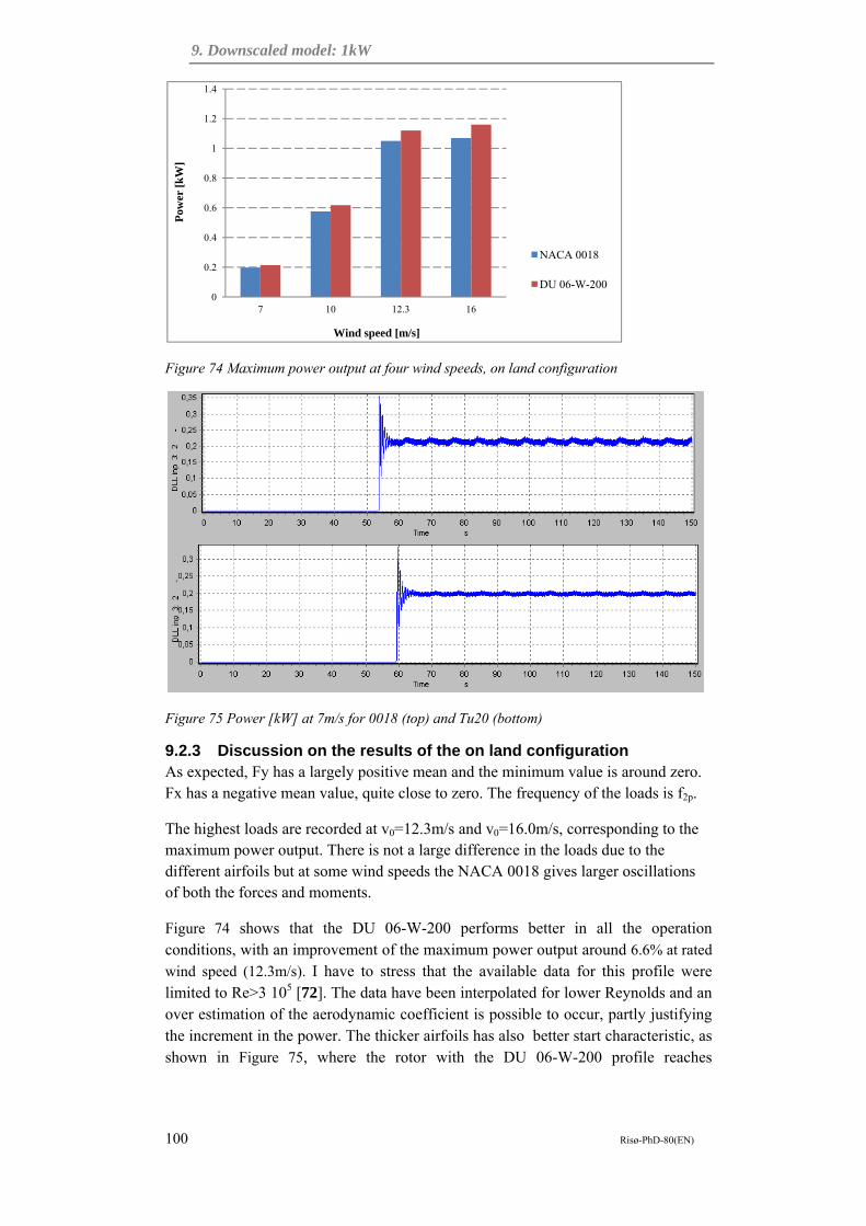
9. Downscaled model: 1kW
100 Risø-PhD-80(EN)
Figure 74 Maximum power output at four wind speeds, on land configuration
Figure 75 Power [kW] at 7m/s for 0018 (top) and Tu20 (bottom)
9.2.3 Discussion on the results of the on land configuration As expected, Fy has a largely positive mean and the minimum value is around zero. Fx has a negative mean value, quite close to zero. The frequency of the loads is f2p.
The highest loads are recorded at v0=12.3m/s and v0=16.0m/s, corresponding to the maximum power output. There is not a large difference in the loads due to the different airfoils but at some wind speeds the NACA 0018 gives larger oscillations of both the forces and moments.
Figure 74 shows that the DU 06-W-200 performs better in all the operation conditions, with an improvement of the maximum power output around 6.6% at rated
wind speed (12.3m/s). I have to stress that the available data for this profile were limited to Re>3 105 [72]. The data have been interpolated for lower Reynolds and an over estimation of the aerodynamic coefficient is possible to occur, partly justifying the increment in the power. The thicker airfoils has also better start characteristic, as shown in Figure 75, where the rotor with the DU 06-W-200 profile reaches
0
0.2
0.4
0.6
0.8
1
1.2
1.4
7 10 12.3 16
Pow
er [k
W]
Wind speed [m/s]
NACA 0018
DU 06-W-200

9. Downscaled model: 1kW
101 Risø-PhD-80(EN)
synchronous rotational speed of the generator faster than the rotor with a NACA 0018 profile.
Eventually, it should be stressed that at high wind speeds, the results are affected by an uncertainty, due to the dynamic stall contribution. Also turbulence might increase those values.
9.2.4 Offshore simulations The rotor and aerodynamic set up is the same used for the on land calculations. In all the simulations I use the profile DU 06-W-200, since it performed better in the previous simulations.
This section includes results from 11 simulations, combining:
- Constant wind speed of 7m/s and 12.3 m/s - Waves of amplitude .4m and period 2s. The wave characteristics have been
reduced considering lower values of v0. The wave directions, w, are 0 and 90 degrees, referred to the wind speed direction.
- Water current of maximum speed 0.1m/s. The current has a power law profile with coefficient 0.5. The directions c of the current are 0 and 90 degrees, referred to the wind speed direction.
The complete list of the simulations is reported in Table 35.
Table 35 Simulations for the offshore configuration
Sim. N. v0 0 Hs TP w c U r
[m/s] [deg] [m] [s] [deg] [deg] [m/s] [rpm]
11 No aerodynamics
5 - - - - - 0
12 No aerodynamics
5 - - - - - 0 - 350
13 7 constant 0 - - - - - 251
14 12.3 constant 0 - - - - - 440
15 7 constant 0 0.45 2 90 - - 251
16 12.3 constant 0 0.45 2 90 - - 251
17 7 constant 0 0.45 2 0 - - 440
18 12.3 constant 0 0.45 2 0 - - 440
19 7 constant 0 0.45 2 0 0 0.1 251
20 12.3 constant 0 0.45 2 0 0 0.1 440
21 12.3 constant 0 0.45 2 0 90 0.1 440

9. Downscaled model: 1kW
102 Risø-PhD-80(EN)
The first two offshore simulations, 11 and 12, do not include aerodynamic loads. I carried out these two runs to verify the dynamic response of the system in absence of aerodynamic loads and evaluated the natural periods in pitch and roll.
The results are shown in terms of dx, dy and dz, displacements of the cross sectional area of the tower at the mean water level. In simulation 11, the turbine is tilted 5 degrees around the x axis, and it is left free to oscillate in the water. In Figure 76 the time series of dx and dy are plotted.
The natural period in pitch and roll are equal and close to 6s, as expected. The roll mode consists only of a vibration mode at the natural frequency. The pitch motion, generated by the inclination of the tower, is larger and quite well damped.
Figure 76Sim11 From top: dx and dy, in meters

9. Downscaled model: 1kW
103 Risø-PhD-80(EN)
Figure 77 Sim12, from the top: 1.r [rpm] 2. Dx [m], 3.dy [m], 4.dz[m]
In sim12, the turbine is also spinning up to 350rpm. In Figure 77, dx, dy and dz are
plotted along with r. The plots allow some observations:
- The natural periods are strongly affected by the rotational speed. At 350rpm, the period of the oscillations is greater than 40s. The same effect is present in both pitch and roll.
- dz, shows a very stiff behavior of the turbine - As expected, at lower rotational speed some high frequency effects are
visible. At high rotational speed, the inertia cancels those effects and the plot appears to be smoother.
- The roll motion generated by the pitch, has a low amplitude, but also a low damping.
The results of the other offshore simulations include:
- Parameters to evaluate the stability of the turbine: mean, max, see Figure 78. These values do not include the deflection of the tower.
- Loads in offshore environment: Mx and My on the mean water level cross section of the tower (point 5), Figure 79.
Time series of the tilt angle are plotted in Figure 80 - Figure 82.
Figure 78 Maximum and mean value of the pitch angle for different offshore external conditions
Sim. 13
Sim. 14
Sim. 15
Sim. 16
Sim. 17
Sim. 18
Sim. 19
Sim. 20
Sim. 21
Pitch angle (mean value) [Deg] 9.28 17.07 11.39 17.18 11.43 18.68 11.38 18.73 17.34
Pitch angle (max value) [Deg] 16.31 23.38 17.85 20.18 18.12 22.42 17.89 22.5 20.11
0
5
10
15
20
25
Pitc
h an
gle
[Deg
]
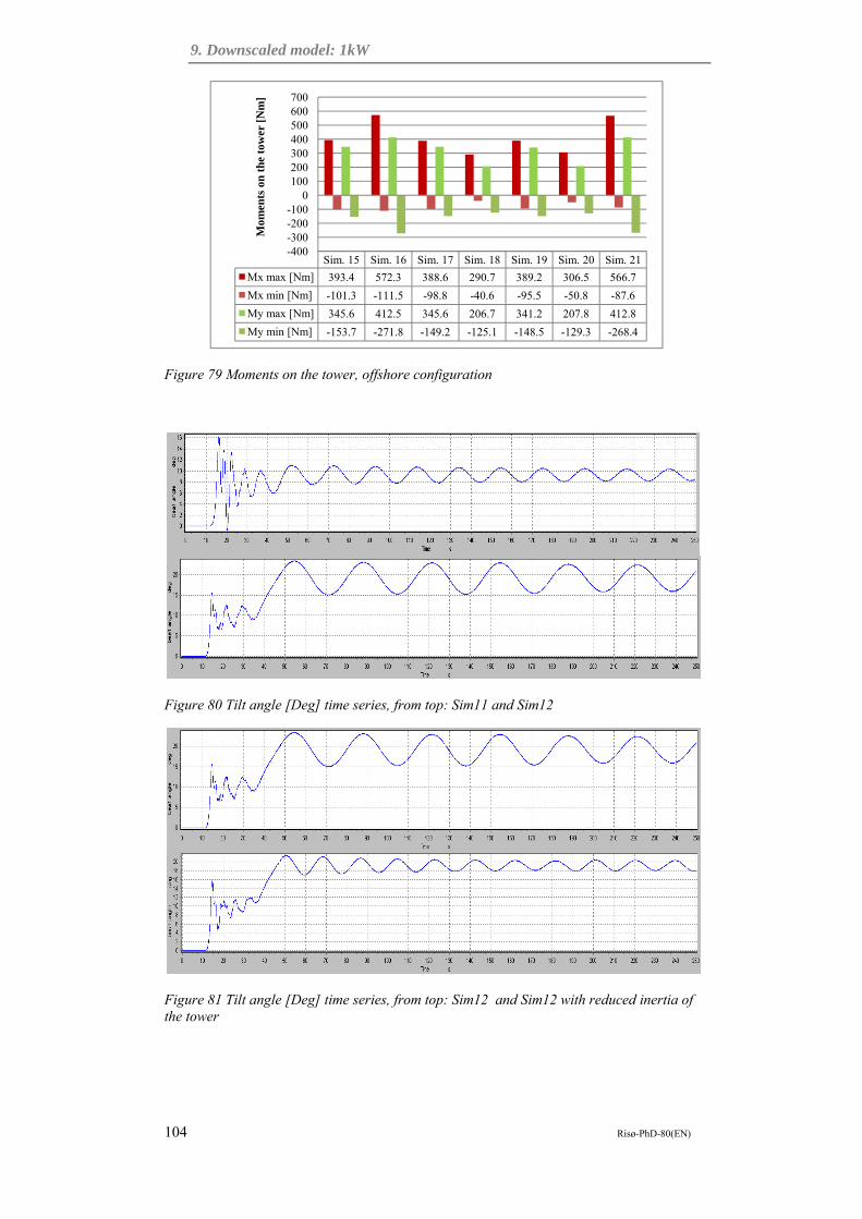
9. Downscaled model: 1kW
104 Risø-PhD-80(EN)
Figure 79 Moments on the tower, offshore configuration
Figure 80 Tilt angle [Deg] time series, from top: Sim11 and Sim12
Figure 81 Tilt angle [Deg] time series, from top: Sim12 and Sim12 with reduced inertia of the tower
Sim. 15 Sim. 16 Sim. 17 Sim. 18 Sim. 19 Sim. 20 Sim. 21
Mx max [Nm] 393.4 572.3 388.6 290.7 389.2 306.5 566.7
Mx min [Nm] -101.3 -111.5 -98.8 -40.6 -95.5 -50.8 -87.6
My max [Nm] 345.6 412.5 345.6 206.7 341.2 207.8 412.8
My min [Nm] -153.7 -271.8 -149.2 -125.1 -148.5 -129.3 -268.4
-400-300-200-100
0100200300400500600700
Mom
ents
on
the
tow
er [N
m]

9. Downscaled model: 1kW
105 Risø-PhD-80(EN)
Figure 82 Tilt angle[Deg] time series. From top: sim17 and Sim18
9.2.5 Discussion on results and recommendations on the platform design
Among the performed simulations, the most challenging one for the equilibrium is at v0=12.3m/s and waves in the same direction as the wind (Sim18 in Figure 79). The water current do not seem to give significant changes (Sim20, in Figure 79).
On the other hand, the most critical loads on the tower, at the mean water level, are recorded for waves or currents perpendicular to the wind speed direction (Sim21 in Figure 79).
The maximum tilt angle do not correspond to the maximum external load, probably due to the strong contribution of the inertial loads.
At low wind speed (7m/s) and 251rpm, the most critical events seem to occur at the starting of the turbine (Figure 80 top). The frequency of the wave loads is still well distinguishable (Figure 82, top).
At v0=12.3m/s and r=440rpm, the periods of the motion in pitch increase strongly (Figure 80, bottom). The contributions of the high frequency loads are less visible (Figure 82, bottom). Meanwhile, the turbine has some larger oscillations, probably due to its inertia.
The loads in Figure 79 are much larger than the loads recorded in the on shore configuration and recorded in Figure 73. However, it is stressed that this may be due to the not scaled effects of the wave-induced loads on the structure, which have a larger relative importance in the downscaled model.
In Figure 81 is shown the importance of the inertia at high rotational speeds. The second plot in the figure is obtained by reducing the inertia of the tower. This causes a strong reduction in the amplitude of the platform oscillations.

9. Downscaled model: 1kW
106 Risø-PhD-80(EN)
9.3 Conclusions The 1kW demonstrator design was first investigated with HAWC2 in on land configuration. The most significant results are:
- The 20% thick airfoil from TuDelft performs better than the NACA0018, based on a power output comparison (around 7% more production), as from Figure 74.
- Some simulations have been carried out at the same conditions investigated in the report from Trento Univeristy [83]. Results from HAWC2 seem quite consistent, as from Figure 75 (top).
Some conclusions have been presented on the loads in offshore configuration:
- Magnus effect seems not to be very relevant, at least in terms of maximum loads.
- The wave loads are quite large and need to be properly modeled. Some experimental results would be recommended to evaluate CD and CM at high rotational speed of the platform.
Aerodynamic loads are dominant for the stability of the platform. The mean value of the longitudinal force (thrust) is the most important parameter.
The periodical variation of the aerodynamic loads, do not affect the equilibrium at high rotational speed
The turbine has equilibrium in pitch, even though it operates at high tilt angles. In the worst condition, the turbine has a tilt angle of 19 degrees, plus fluctuations
The design has been verified with simulations in HAWC2:
- The inertial loads seem to be very important at high rotational speeds and the natural periods are larger than expected. (Figure 77, Figure 80, Figure 81).
- Due to the high frequencies, the periodical aerodynamic loads are not a problem for the stability (Figure 77).
- High rotational speeds and thrust give important values of the tilt angle.
Some limitations of this study should be mentioned:
- Aerodynamic load calculation may change with turbulence effects.
- Dynamic stall can also affects the results at high wind speeds.
Last, some recommendations for possible future work:
- A choice about the anchoring system should be made. Some considerations on this issue are:
To have a positive restoring contribution in pitch, the attachment of the mooring lines has to be above the centre of gravity. This would require a new modification of the design either the use of a bearing around the tower.

9. Downscaled model: 1kW
107 Risø-PhD-80(EN)
In case the mooring lines are not taking any moment, the attachment could be placed at the bottom of the structure.
- In order to improve the stability of the platform, some new configurations for the offshore design could be considered, i.e. conical shaped tower. Other solutions found in the literature have also been mentioned.

10. Cost models for floating offshore wind turbines
108 Risø-PhD-80(EN)
10 Cost models for offshore floating wind turbines
The economics of wind-generated electricity can be studied from two different points of view: the cost to produce electricity and the value of the same electricity in the energy market. The first one addresses mainly technical and financial issues, while the second deals with social and political aspects. The two problems are obviously coupled, but in my dissertation I will consider the production cost (the first of the two mentioned approaches) of wind energy as an independent problem.
In this chapter I organize my research in two tasks:
- A survey of studies carried out in the past ten years - A preliminary evaluation of the concept based on the present possibilities.
First, I introduce some terms which are commonly used in economical studies.
The levelized cost of energy (COE) is defined as:
·
Where
FCR is the fixed charge rate and depends on the currency in which the cost is calculated
ICC is the initial capital cost, corresponding to all the expenses at the moment of the wind farm installation. This term includes the cost of the turbine (rotor and tower), drive train and electrical components (generator, bearings, brakes transformer, cabling and electrical connection), balance of station (foundation, transportation, installation, permits). For offshore wind energy it will additionally include: anchoring and platform, harbour facilities and infrastructure, scour protection, marine operation, special additional permits, proper material treatment for marine environment, use of offshore technologies for installation and decommissioning.
AEP is the net annual energy production.
AOE is the annual operating expenses, mainly consisting of levelized O&M cost: AOE=O&M/AEP. Additional annual expenses connected to permits, leasing and replacement of components can be added.
10.1 Cost analysis of wind energy There are essentially two possible approaches to evaluate the cost effectiveness of wind turbine concepts: the first is based on statistical data and quotations from

10. Cost models for floating offshore wind turbines
109 Risø-PhD-80(EN)
manufactures; the other one is a design model where the data are acquired with an engineering numerical calculation, [85]. The last model has the advantage to be more accurate and adaptable to estimate cost effectiveness of new technological concepts. On the other hand it is usually quite complex and requires a team of expertise to be built and also to be run. The statistical model gives less flexibility in the design phase but it has the high advantage that, after compiled, it can be easily used also by not expert customers.
In the US, a project called WindPACT (Wind Partnership for Advanced Component Technology) was performed to predict cost projections for wind turbine upscaling. The results were grouped in several reports dealing with different terms of the cost of energy (such as composite blades for 80-120m rotors [66], base of station, alternative drive train, rotor and tower). WindINPACT project was not directly providing prices of the wind electricity production, but it was rather giving an estimation of the impact of new technologies on the mass and cost of wind turbine components. Cost functions were developed to scale the cost and the mass of the wind turbines. Starting from WindINPACT reports, NREL has developed a cost model to predict cost of wind-generated electricity [65]. The model essentially consists of a spreadsheet which predicts the COE of a wind farm using simple formulas to calculate each term of a wind farm cost. The formulas are obtained by analysis of statistical data (mainly for wind turbines up to 2MW) and using the upscaling functions from WindINPACT projects (for wind turbines larger than 2MW). One of the problems in developing this kind of model is to have a result durable in the time, which is not affected by financial variables. To overcome this limitation the cost models commonly include economic parameters, such as the inflation rate. NREL model uses the Produce Price Indexes (PPIs) rather than the inflation index. The PPI is released yearly from the US federal government and takes into account the prices of the materials from different industries in the U.S. The PPI is more accurate than the inflation index because it considers the variability of the cost linked to the production cost and to the availability of the rough materials. These indexes can be used only backwards in time to adjust the present prices on the older values, but it cannot be used to forecast future cost of the materials. Another limitation of the model is that, due to the statistical approach of the calculations and to the lack of offshore data, the model is mainly intended for onshore wind energy.
In Netherlands an advanced cost model had been developed specifically for offshore wind energy, within the DOWEC project (Dutch Offshore Wind Energy Converter), [74]. The project was carried out by a consortium and the model follows an approach similar to the one from NREL. All the relevant costs for the complete development of a wind farm were listed and the breakdown of the total cost was obtained. Then the data on the expected costs of each sub-component and sub-action were collected from different partners and reported in a spreadsheet. Finally all the costs are summed up again and used with the AEP and the financial parameters, to calculate the COE. DOWEC emphasizes particularly the importance of the coupling between a cost model and the design of the wind turbines, in order to estimate the cost effectiveness of a new concept design. The project included the design of a baseline 6MW HAWT, to use for evaluating the effect of new design concepts on the COE. The cost model is re-used at each design step, to integrate the cost analysis with the

10. Cost models for floating offshore wind turbines
110 Risø-PhD-80(EN)
technical improvements. An example of the application of this approach is given by Hendriks in the evaluation of different control strategies for HAWT (pitch and stall controls), [86].
Another study on the cost of offshore wind-generated electricity is available in a report from Garrad Hassan, [87]. The study aims at the calculation of the cost of energy production per installed MW but addresses that this value can be largely dependent to the technological concept. The major uncertainty results in the assessment of the O&M costs, which represents a considerable amount in the breakdown of the total cost for an offshore wind farm, i.e. 28% according to [45]. This is mostly due to the lack of available statistical data, which are essential for evaluation of O&M expenses. Another uncertainty in the estimation of the cost of the sub-components and sub-actions is due to the immature state of some technological elements. To overcome this limitation, in the report a progress ratio approach is used, estimating the future reduction in the cost due to technological upscaling, scale in the production and learning process. The report estimates a reduction in the cost of 15% in the short term. Using the same approach Juginger forecast a cost reduction up to 39% in 2020. The 80% of the improvement in cost effectiveness is supposed to come from mutual learning in the different technologies involved in the offshore wind energy [88].
An attempt to evaluate floating offshore wind turbine concepts has been carried out by Wayman [89]. She based her estimations on the capital cost of the considered concepts, disregarding O&M cost and the relevance of financial parameters.
As a conclusion of this overview on the wind energy cost models, I would like to quote Zaaijer from TUDelft: “There is no such thing as ‘the one cost model for offshore wind energy’ […] the cost model must match the target of the application” [85].
10.2 DeepWind evaluation So far, none of the described models is applicable to the DeepWind concept for limitations of the models (regarding both VAWTs and floating foundations) and for the limited development of the concept itself. At the current state of development an estimation of the COE would be pure speculation because the uncertainties in all aspects of parameter estimation would be extremely high. Therefore I have preferred to use a concept to concept comparison as evaluation method.
In my dissertation I consider neither financial nor socio-economic parameters, since I assume that these variables do not affect the value of a concept with respect to another one. I have also decided to not include the O&M costs because of their high variability. This is a strongest assumption, but I consider that in the evolution of new concepts, the ICC is still the most relevant parameter. Therefore I only focus at the capital cost ICC of the EOC formula (64% of the wind farm costs), and I consider the following shares [74]:
- Installation cost (17.2%), including assembly, transportation and installation. - Hardware cost (82.8%), including, rotor, tower, platform and generator box.

10. Cost models for floating offshore wind turbines
111 Risø-PhD-80(EN)
I consider the hardware costs divided in:
- Rotor (20.1%), including hub, blades and pitch control system. - Support structure (35.6%), consisting of tower and foundation (or platform).
There is no reference on the breakdown of these costs between platform and tower. Here I consider the platform to be the 70% of the support structure costs (24.92% of the hardware costs) and the tower the 30% (10.68%)
- Nacelle (25.1%), including generator, gear box and all the sub-components housed in the nacelle.
- Other costs (19%), which are expenses not directly connected to the wind turbine concept, as the electric collection system and the transmission system to shore.
I have selected as a comparative model, OC3-Hywind 5MW design, as described in [44]. There are some clear advantages in this choice. First, Hywind is a good baseline model for a comparison, since it is a proven concept close to commercialization. Moreover the similarity between the two concepts allows some simplifications and reduces the uncertainties on the results. I consider the cost of a single wind turbine, since there are not sufficient data to evaluate the impact of the different concepts in a wind farm layout.
Table 36 Main characteristics of the two concepts. *the data are taken from [44], [28] and [43]
Parameter OC3-Hywind* DeepWind Rated Power [MW] 5 5 Rated rotational speed [rpm] 12.1 5.26
Rated wind speed [m/s] 11.4 15 Tower elevation [m] 97.6 145 Tower weight [kg] 3.47 105 4.45 105 Blades length [m] 61.5 188.68 Weight of 1 blade [kg] 1.77 104 1.58 105
Number of blades [-] 3 2 Blade chord [m] 4.65 – 1.42 (tapered) 7.45 Draft of the platform [m] 120 110 Platform water displacements [m3] 8029 5940
Control systems [-]
Pitch regulation + yaw system
Rotational speed regulation
In order to start, I had to make a further assumption, considering the costs breakdown above valid for both the two wind turbine concepts. I compare the cost of each sub-component in the two concepts.
When it is possible, I base the comparison on available data, such as the mass.
When detailed data are not available, I compare the sub-components using theoretical considerations. Then I rate each sub-component of the VAWT with respect to the respective HAWT component. When my comparison is based on a pure theoretical evaluation, I use 6 possible grades for the evaluations: highly unfavourable, unfavourable, slightly unfavourable, neutral, slightly favourable,

10. Cost models for floating offshore wind turbines
112 Risø-PhD-80(EN)
favourable, highly favourable. These correspond to a percentage variation in the cost, supposed to be respectively: -100%,-50%, -10%, 0%, 10%, 50%, 100%, see Table 38.
ROTOR
The blades for Deepwind are 3.07 times longer and even though only two blades are needed, the value of the weight ratio is larger. Indeed the weight of the two VAWT blades results in 5.95 times the total weight of the three HAWT blades (without including the hub). In his study on HAWTs blades, Cheney states the reduction in the cost due to pultrusion process to be up to 74%, [90]. In another investigation on pultruded blades for HAWTs, the cost of pultruded blades is indicated to be for the 97.74% linearly dependent from the mass, [46]. Therefore, supposing a unitary cost Cblades_H for the three HAWT blades, the relative cost Cblades_V of the VAWT blades is:
1 0.74 0.0226 0.9774 · 5.95 1.518
Then I rated as unfavourable the production of VAWT blades.
However the breakdown of the cost of a HAWT rotor shows that the blades represent only 43% of the total rotor cost, with the other 57% consisting of the hub and pitch control system [74]. These two costs are not present in a VAWT design, therefore I consider the total relative cost of the rotor as:
0.43 · 1.518 0.65
TOWER
Both the towers are built in steel and, considering the cost proportional to the weight of the structure, I obtain:
4.453.47
1.28
I have to stress at least two possible sources of errors:
- The weights have been calculated using different properties for the steel. Indeed the Hywind OC3 is designed considering a density of 8500kg/m3, instead of the typical value of 7850kg/m3 used in my work. The reason of the higher values is to account for the weight of other parts, such as flanges and welds.
- I consider a more conservative value for the clearance of the blades from the water, i.e. 15m instead of 10m. This is mainly due to avoid any possible problems in the calculations but a lower value could be considered. Additionally, the VAWT tower can still be optimized reducing the radius of the height.
Both these two observations are valid also for the discussion on the platform, since the weight distribution has a strong influence on the design of the underwater structure.

10. Cost models for floating offshore wind turbines
113 Risø-PhD-80(EN)
GENERATOR BOX
Here I consider the elements housed in the generator box, which usually for a HAWT are grouped with the name “nacelle costs”. I considered some of the costs to be insensitive to the type of design, such as the computer, the sensors and the electrical converter. These costs make up to 38.5% of the total.
I considered as costly unfavourable for a VAWT, the following sub-components:
- The housing (originally the 2% of the cost), which has to deal with underwater pressure and corrosion. I applied an increasing ratio of 100%.
- The bearings, since they have to take a considerable axial load varying with the time. In HAWT breakdown this cost is set very close to zero, therefore I considered it as part of the generator costs.
- The generator, including gear system, makes up to 52% of the cost and it could in principle be the same for the two concepts. However, some distinctions have to be made. Placing the generator in the bottom, the VAWT has no limitation on the weight of the generator. A direct drive variable speed generator could be used saving the costs of the gear box. On the other hand, some limitations could occur in space. Indeed, the low rotational speed of the rotor makes the dimensioning of the generator to be challenging. Eventually also the cost of the bearings has to be included. An accurate prediction on these costs would require a deep investigation considering several aspects. Therefore, due to the large number of uncertainties, I have chosen a conservative approach, with an increase of 50% in the generator costs.
- The brake system has to be capable to stop the turbine without the support of aerodynamic brakes. Water brakes could solve this problem and cut the costs. Meanwhile I consider these costs to be doubled in a VAWT design. The original share of the brakes in the costs breakdown of a HAWT is 2.5%.
The yaw system, consisting of the 5% of the total cost, is not needed in a VAWT.
Table 37 Cost of the sub-components housed in the generator box.
Generator housing Cost in percentage
Ratio
Housing 2 Highly unfavourable 2 Generator (included gear system and shaft)
52 Unfavourable 1.5
Yaw system 5 Not present 0 Bearings <1 Highly unfavourable - Computer and sensors
26.5 Neutral 1
Electrical conversion 5 Neutral 1 Brake system 2.5 Highly unfavourable 2 Electrical cables 4.5 Neutral 1 miscellaneous 2.5 Neutral 1 TOTAL 1.219

10. Cost models for floating offshore wind turbines
114 Risø-PhD-80(EN)
The total cost of the components housed in the generator box is then:
0.385 .52 · 1.5 0.02 · 2 .025 · 2
1.219
PLATFORM AND ANCHORING
I considered as unchanged the costs for mooring lines and anchors. A best evaluation would require a tailored design of DeepWind according to the 3rd configuration of 2.6.3.
For the platform I considered the same approach used for the tower, considering the cost to be directly proportional to the water displacements. Then it is:
59408029
0.74
INSTALLATION
As described in 2.3.1, DeepWind allows some better possibilities for installation procedure, especially at sites where the turbine has to be tilted up with the rotor already mounted. Meanwhile, no VAWT has ever been installed offshore and an additional cost connected to the learning process should be considered in the first years. Eventually I rated as slightly favourable DeepWind configuration for the installation.

10. Cost models for floating offshore wind turbines
115 Risø-PhD-80(EN)
Table 38 Cost comparison of different sub-components of the capital costs.
Sub-component From OC3Hywind to DeepWind
Cost ratio DeepWind/OC3Hywind
ROTOR 0.65 Blades Unfavourable 1.518 Hub and Picth control
Not present -
TOWER 1.28 Tower structure Unfavourable 1.28 GENERATOR BOX
1.219
Housing Unfavourable 2.0 Generator Unfavourable 1.5 Yaw system Not present - Bearings Highly unfavourable (included in the generator) Computer and sensors
Neutral 1.0
Electrical conversion
Neutral 1.0
Break coupling system
Highly unfavourable 2.0
Electrical cables Neutral 1.0 miscellaneous Neutral 1.0 OFFSHORE STRUCTURES
0.74
Platform Favourable 0.74 INSTALLATION 0.9 Transportation Slightly favourable 0.9 Installation Slightly favourable 0.9
Summing up the values in Table 39, I obtain a relative cost factor of 0.93, meaning a 7% reduction of the capital costs in using DeepWind concept. This preliminary study allows considering DeepWind as a possible competitive concept in a market where Hywind is close to become commercial. Nevertheless, particular care is recommended in use of these values as a demonstration of possible concept superiority. There are still too many uncertainties, which don’t allow any further and definitive conclusion. Among these uncertainties, the most relevant are:
- The analysis of different offshore concepts is very dependent from the site and a cost analysis should be made considering different sites with a considerable number of available data
- The turbines are designed for different rated wind speeds and with a different control system. Thus the AEP is very different (higher for the HAWT design). Also the design of the rotor should be tailored on the site to maximize the AEP.
- The VAWT design has not been optimized, as the HAWT. Some additional iteration in the design process, which would include more detailed descriptions of the components, could reduce the gap in the AEP. A better study on the control possibilities would also better clarify which control strategy can be applied to increase the energy efficiency.

10. Cost models for floating offshore wind turbines
116 Risø-PhD-80(EN)
- The properties used to describe the materials are not the same, as I have mentioned for the steel. And also the safety factors applied on the structure seem to be different.
- The design of the VAWT is mainly thought to use the technologies available on the market nowadays. These technologies have been mostly meant to work on HAWTs and in the future more tailored product for VAWTs could be available.
Table 39 Summation of the sub-components costs
Original share in offshore HAWT wind farm
DeepWind adaptation factor
Final weight compared to OC3Hywind
Rotor 0.17 0.65 0.11 Generator box 0.21 1.22 0.25 Tower 0.09 1.28 0.11 Platform 0.21 0.74 0.15 Other costs 0.16 1.00 0.16 Installation 0.17 0.90 0.15 TOTAL 1.00 0.93

11. Conclusions
117 Risø-PhD-80(EN)
11 Conclusions My work aimed at investigating the feasibility and the potential of a new offshore floating vertical axis wind turbine concept. Driven by this goal, the study has gone through a broad range of disciplines and technological problems. At the end of my dissertation, the state of the knowledge on this new concept is increased thank to new results and meantime additional questions emerged during the study, addressing the need for further investigations.
The most relevant conclusions for the concept evaluations are:
1. The new concept has its greater favourable characteristic in its simplicity. This allows different possible configurations, for example for the rotor and the anchoring system. In the selection of the first configuration to study I followed the approach used by Hendriks to design a baseline HAWT turbine [45]. Since this first design has possibly to be a reference for future calculations and modifications, it has to be based as much as possible on known and proven technology. Following this criteria, the first design decisions have been taken in Chapter 2.
2. From the analysis of the loads, it is emerged the preponderance of the hydrodynamic loads for the stability of the system. This result is extendable to other floating wind turbine concepts and it is consistent with the previous studies. It also means that both the feasible and the optimal design of floating wind turbines are strongly dependent from the site.
3. The coupling between the design and the external conditions is even more evident in DeepWind concept because the rotation of the platform generates new loads, such as a lateral force (Magnus effect), a drag force and a friction moment. The forces and the moment generated by a water stream passing the rotating platform have been numerically computed in Chapter 4. To my knowledge this study has two novelties: the application of these loads to the platform of a wind turbine and the large values of the Reynolds number
(>106) combined to the large number of (>2), where is the ratio of the peripheral speed and the velocity of the water stream. The results show values of the lateral force very close to the value found at lower Reynolds numbers (Re~104) by other authors. These results were expected at high rotational speed, since in both cases Re is larger enough to avoid the separation of the boundary layer. It was unexpected to me the presence of a
negative drag (thrust) at large values of This result needs further investigation and it could affect the platform stability. The friction seems to represent a minor problem in the design, but marine growth could make it worst. Therefore, even though the friction doesn’t represent a significant limit in power production, it could result in an undesired increase in O&M costs.
4. The concept has been tested using the numerical code HAWC2, developed at Risø DTU and capable in handling very different concepts, such as

11. Conclusions
118 Risø-PhD-80(EN)
floating VAWTs. To achieve an acceptable accuracy in my simulations, I added some DLLs to the code, simulating the VAWT aerodynamics and the hydrodynamic loads on the rotating structures. A first 2MW design has been used as a test model to verify the proper functionality of the software and the correct coupling of all hydro and aero- dynamics.
5. A 5MW concept has been designed and tested with HAWC2. The design addressed some challenges, for example in dimensioning of very large blades with constant properties over the length (hypothesis due to the pultrusion process). The large dimensions of the platform results mainly in a regime dominated by inertial forces, apart for the most critical sea states, which generates large KC numbers and significant viscous effects. The
turbine has been designed to run with a tilt angle lower than 10 degrees, in most of the operative conditions, to avoid major structural problems. I carried out simulations at three sea states and for different directions of the currents and of the waves propagation. The turbine operates with a tilt angle
depending on the external conditions. When the turbine is in equilibrium (in absence of large variations of the external conditions) the platform
oscillates around the equilibrium value of and describes an elliptical motion, due to the precession mode of the turbine. The motion of the turbine in the mean water plane is strongly coupled in the x and y axes. Indeed the turbine is subjected to gyroscopic effects generated by the rotation and to the hydrodynamic lateral force generated by the relative motion of the platform respect to the water. From the simulations, the turbine exceeds the inclination of 10degrees ( 12degrees) only for two particular combinations of wave, wind and currents directions. However I didn’t register any significant deformation of
the tower due to the high tilt angle. The greater values of are due to the currents acting perpendicularly to the wind, resulting in a hydrodynamic force on the same direction of the hydrodynamic thrust. The hydrodynamic loads of the currents and the aerodynamic loads have the same magnitude order and when they act on the same direction, the turbine operates close to the vertical position. The dynamic contribution of the waves results in larger amplitudes of the motion of the turbine and in increased loads on the structure.
6. I designed also a 1kW model for experimental investigations. The typical scale factors applied in offshore modelling are described in Chapter 5. However these scale factors cannot be applied without to adjust the rotor design. I eventually decided to design the 1kW floating VAWT, as a small version of the concept rather than as a downscaled model of a 5MW turbine. This is also due to practical reasons in manufacture the small turbine and to the real conditions at the site, which cannot be scaled as a downscaled model would require. A small model, even though not reproducing exactly a larger design, can give important clarifications on the feasibility of the concept (such as the possibility of using the water as a roller bearing) and can possibly address new relevant aspects to investigate. The design of the turbine has been conditioned by the limited depth of the Roskilde fjord. For such shallow waters, the draft of the platform cannot exceed 2.7m and the

11. Conclusions
119 Risø-PhD-80(EN)
turbine is designed to operate at high tilt angle . The numerical simulations confirm this data and show a strong influence of the rotor inertia on the dynamics of the platform. The natural periods of the pitch and roll modes are much larger than expected and I believe this is due to the high rotational speeds. Due to the high rotational speed the stability of the platform is not affected by the strong periodic variation of the aerodynamic loads. Another peculiarity of the small model is that the aerodynamic loads are dominant over the other loads and the turbine is constantly tilted in the wind direction. The Magnus effect doesn’t give significant contribution, due to the low speed of the currents at the site.
7. From my investigation it emerges that there is a large numbers of variables to consider in the study of DeepWind concept and the design space is very narrow. However, I did not find any serious issue, which could invalidate the feasibility of the concept and from a first outlook there are good economical potentials.
The need for further work emerged during this study and I grouped some of the most urgent key aspects, which should be developed first:
1. Due to the novelty of the concept I experienced a lack of appropriated standards. Nothing is specified about the characterization of the vertical water current profile and only small attention is dedicated to turbulence of the water stream and the direction of the currents with respect to the waves. Other limits regard the rotor standards, since VAWTs are not included in the wind turbine standards [49], [76].
2. Other improvements can come from a more precise characterization of the met-ocean conditions at the site. A correct evaluation of DeepWind concept would require a joint of wind, waves and currents data. Additionally, the vertical variation of the currents should be measured, including the velocity and the currents direction.
3. The implementation of the aerodynamic code in a DLL offered some advantages during the development process. However, for further investigations, the integration of the aerodynamic routine in the main code is recommended to decrease the computation time, reduce the number of input files and allow the use of all the features included in the main program (as turbulence, dynamic stall and tower shadow effects).
4. Possible design variations to the concept could be tested: straight blades can allow pitch control and lower the weight, 3 blades to reduce the periodic loads, longer rotor to reduce the cost and the gyroscopic effects. Investigation of the second and third configurations should come parallel to the new design concepts.
5. The rotation in water of the rotor affects the natural frequencies of the system. This can be an important issue to investigate, especially for the demonstrator.
6. The design of the blades for large rotors is resulted to be challenging. Here, I proposed to use to different sections over the blade, even though without changing the chord. Other designes are possible and some further studies are

11. Conclusions
120 Risø-PhD-80(EN)
needed, taking three variables into account: the structural strength of the blade, the manufacture feasibility and the costs.
7. The design of the generator for the 5MW DeepWind concept has to deal with some particular constraints, such as the placement in deep water and the very low rotational speed. The weight is not a limitation in the design, but the dimensions could create problems in dimensioning the platform. An option could be to use more than one generator, for example two 2.5MW generators.
8. Beyond the evaluation of this concept, there is need for new cost models capable to evaluate floating wind turbine concepts. I would distinguish between two possible models. A specific simplified cost model could be useful in the design process of DeepWind concept, to evaluate the possible technological solutions and modifications applicable to the baseline model. Another model could be used to evaluate different floating wind turbine concepts. As learnt from literature a cost model with this potential cannot be exclusively based on statistical data, but it needs an engineering model and a baseline design to use as reference [45], [85]. Both the tasks are challenging due to the many differences among the floating wind turbine concepts describe in Table 2.

Bibliography
121 Risø-PhD-80(EN)
Bibliography [1] L. Vita, U. S. Paulsen, T. F. Pedersen, H. A. Madsen, and F. Rasmussen, "A
novel floating offshore wind turbine concept," in Proceedings of the European Wind Energy Conference (EWEC), Marseille, France, 2009.
[2] U. S. Paulsen, T. F. Pedersen, and L. Vita, "Existing VAWT technologies," Risø DTU (Technical University of Denmark), Roskilde, Denmark, I-2613(EN), 2008.
[3] U. S. Paulsen, T. F. Pedersen, L. Vita, H. A. Madsen, and F. Rasmussen, "Recommendations for floating VAWT technology demonstration and development," Risø DTU (Technical University of Denmark), Roskilde, Denmark, I-2616(EN), 2008.
[4] A. Zervos and C. Kjaer, "Pure Power - Wind Energy scenarios up to 2030," European Wind Energy Association (EWEA), 2008.
[5] N. Fichaux and J. Wilkes, "Oceans of opportunity," European Wind Energy Association (EWEA), Brussels, Belgium, 2009.
[6] S. Krohn, P. Morthorst, and S. Awerbuch, "The economics of wind energy," European Wind Energy Association (EWEA), Brussels, Belgium, 2009.
[7] G. J.M. Darrieus, "Turbine having its rotating shaft transverse to the flow of the current," 1835018, 1926.
[8] D. Coiro, F. Nicolosi, A. De Marco, S. Melone, and F. Montella, "Dynamic behaviour of patented Kobold tidal current turbine: numerical and experimental aspects," in Proceeding of the 4th International Conference on Advanced Engineering Design, Glasgow, UK, 2004.
[9] T. D. Ashwill and T. M. Leonard, "Developments in blade shape design for a Darrieus vertical axis wind turbine," Sandia National Laboratories, Albuquerque, New Mexico (US), SAND86- 1085, 1986.
[10] R. E. Sheldal, "Comparison of field and wind tunnel Darrieus wind turbine data," Sandia National Laboratory, Albuquerque, New Mexico (US), SAND80-2469, 1981.
[11] B. F. Blackwell, Robert E. Sheldahl, and Louis V. Feltz, "Wind tunnel performance data for the Darrieus wind turbine with NACA 0012 blades," Sandia National Laboratory, Albuquerque, New Mexico (US), SAND76-0130, 1977.
[12] R. E. Sheldal, P. C. Klimas, and L. V. Feltz, "Aerodynamic performance of a

Bibliography
122 Risø-PhD-80(EN)
5-metre-diameter turbine with extruded alluminum NACA 0015 blades," Sandia National Laboratories, Albuquerque, New Mexico (US), SAND80-0179, 1980.
[13] T. D. Ashwill, "Measured data fore the Sandia 34-meter vertical axis wind turbine," Sandia National Laboratories, Albuquerque, New Mexico (US), SAND91-222, 1992.
[14] T. D. Ashwill, "Initial structure response measurements and model validation for the Sandia 34-Meter VAWT test bed," Sandia National Laboratories, Albuquerque, New Mexico (US), SAND88-0633, 1990.
[15] T. G. Carne and A. R. Nord, "Modal testing of rotating wind turbine," Sandia National Laboratories, Albunquerque, New Mexico (US), SAND82-0631, 1983.
[16] D. E. Berg, "Structural design of the Sandia 34-meter vertical axis wind turbine," Sandia National Laboratories, Albequerque, New Mexico (US), SAND84-1287, 1985.
[17] M. E. Ralph, "Design and Control of the variable speed generator on the Sandia 34-meter vertical axis wind turbine," in Proceedings of the Windpower Conference, San Francisco, California (US), 1989, pp. 55-59.
[18] FloWind Corporation, "Final project report: high energy rotor development, test and evaluation," Flowind Corporation, Sandia Contract AB-7292, San Rafael, California (US), SAND96-2205, 1996.
[19] P. W. Carlin, A. S. Laxson, and E. B. Muljadi, "The hystory and state of the art of variable speed wind turbine technology," Wind Energy, vol. 6, pp. 129-159, 2003.
[20] I. Paravischivoiu, Wind turbine design, with emphasis on Darrieus concept.: Polytechnic International Pres, 2002.
[21] C. Beller, "Urban wind energy - state of the art 2009," Risø DTU (Technical Universitry of Denmark), Roskilde, Denmark, Risø-R-1668(EN), 2009.
[22] Renewable Energy 2010 target Team Business Development Unit, "The world offshore renewable energy report 2004-2008," London (UK), 2008.
[23] A. R. Henderson and David Witch, "Floating offshore wind energy - A review of the current status and an assesment of the prospects," Wind Engineering, vol. 34, no. 1, pp. 1-16, 2010.
[24] W. Musial and B. Ram, "Large-scale offshore wind power in the United States - Assesment of opportunities and barriers," National Renewable Energy Laboratory, Golden, Colorafo (US), NREL/TP-500-40745, 2010.

Bibliography
123 Risø-PhD-80(EN)
[25] W. Musial and C. Butterfield, "Future for offshore wind energy in the United States," in Proceedings of the Energy Ocean Conference, Palm Beach, FL, 2004.
[26] W. Stoddard, "The life and work of Bill Heronemus, wind energy pioneer," Wind Engineering, vol. 26, no. 5, pp. 335-341, 2002.
[27] O. M. Faltinsen, Sea loads on ships and offshore structures.: Cambridge University Press, 1990.
[28] J. Jonkman and D. Matha, "Dynamics of offshore floating wind turbines - analysis of three concepts," Wind Energy, vol. 14, no. 4, pp. 557-569, 2011.
[29] PrinciplePowerInc., "Column-Stabilized Offshore Platform with Water-Entrapment," WO2009131826.
[30] B. Skaare et al., "Integrated dynamic analysis of floating offshore wind turbines," in Proceedings of the Euorpean Wind Energy Conference (EWEC), Milan, Italy, 2007.
[31] J. Jonkman, "Dynamics modelling and load analysis of an offshore floating wind turbine," National Renewable Energy Laboratory, Golden, Colorado (US), Ph.D. Dissertation NREL/TP-500-41958, 2007.
[32] I. Ushiyama, K. Zechi, and H. Miura, "A feasibility study for floating offshore windfarms in Japanese waters," Wind Engineering, vol. 28, no. 4, pp. 383-398, 2004.
[33] T. J. Larsen and T. D. Hanson, "A method to avoid negative damped low frequent tower vibrations for a floating, pitch controlled wind turbine," in Proceedings of the Conference The science of making torque from the wind, Copenhagen, Denmark, 2007.
[34] J. E. Withee, "Fully coupled analysis of a floating wind turbine system," MIT (Massachussets Institute of Technology), Cambridge, Massachussets (US), PhD Thesis 2004.
[35] K. H. Lee and P. Sclavounos, "Floating wind turbines," in Proceedings of the 20th Workshop on Water Waves and Floating Bodies, Spitsbergen, Norway, 2005.
[36] J. H. Strickland, "The Darrieus turbine: a performance prediction model using multiple streamtubes," Sandia National Laboratories, Albuquerque, New Mexico (US), SAND75-0431, 1975.
[37] H. A. Madsen, "On the ideal and real energy conversion in a straight bladed vertical axis wind turbine," Aalborg University Centre, Aalborg, Denmark, Ph.D. Report ISBN: 87-87681-06-4, 1983.

Bibliography
124 Risø-PhD-80(EN)
[38] T. J. Larsen and A. M. Hansen, "How 2 Hawc2, the user's manual," Wind Energy, Risø DTU (Technical University of Denmark), Roskilde, Denmark, Risø-R-1597, 2009.
[39] J. Jonkman et al., "Offshore code comparison collaboration within IEA wind task 23: Phase IV results regarding floating wind turbine modelling," in Proceedings of the European Wind Energy Conference (EWEC), Warsaw, Poland, 2010.
[40] L. Vita, U. S. Paulsen, T. F. Pedersen, H. A. Madsen, and F. Rasmussen, "DeepWind: a novel floating offshore wind turbine concept," WindTech, vol. 6, no. 4, 2010.
[41] J. N. Newman, Marine Hydrodynamics.: Massachussets Institute of Technology, 1977.
[42] L. Vita et al., "A novel concept for floating offshore wind turbines: recent developments in the concept and investigations on fluid interaction with the rotating foundation," in Proceedings of the International Conference on Ocean Offshore and Arctic Engineering (OMAE), Shanghai, China, 2010.
[43] J. Jonkman, S. Butterfield, W. Musial, and G. Scott, "Definition of a 5-MW reference wind turbine for offshore system development," National Renewable Energy Laboratory, Golden, Colorado (US), Technical Report NREL/TP-500-38060, 2009.
[44] J. Jonkman, "Definition of the floating system for phase IV of OC3," National Renewable Energy Laboratory, Golden, Colorado (US), Technical report NREL/TP-500-47535, 2010.
[45] H. B. Hendriks and alt., "Cost modelling aspects in the design of an offshore wind turbine," in Proceedings of the Offshore wind energy special topic conference, Brussels, Belgium, 2001.
[46] P. G. Migliore and M. C. Cheney, "Feasibility study of pultruded blades for wind turbine rotors," in Proceedings of the ASME/AIAA Wind Energy Symposium, Reno, Nevada (US), 2000.
[47] B. F. Blackwell, "The Vertical Axis Wind Turbine, "how it works"," Sandia National Laboratories, Albuquerque, New Mexico (US), Patent Caution SLA-74-0160, 1974.
[48] B. M. Sumer and J. Fredsøe, Hydrodynamics around cylindrical structures.: World Scientific, 2006.
[49] IEC 61400 – 3 Ed.1, "IEC 61400 – 3 Ed.1: Wind turbines – Part3: Design requirements for offshore wind turbines," 2008.

Bibliography
125 Risø-PhD-80(EN)
[50] B. M. Sumer and J. Fredsøe, Hydrodynamics around cylindrical structures.: World Scientific, 2006.
[51] R. Monti and R. Savino, Aerodinamica. Napoli: Liguori Editore, 1999.
[52] L. Prandtl, "Die Naturwissenschaften (Application of the Magnus effect to the wind propulsion of ships," NACA, Tech Mem. 387, vol.13, 1926.
[53] S. Mittal and B. Kumar, "Flow past a rotating cylinder," Journal of fluid mechanics, vol. 476, pp. 303-334, 2003.
[54] J. C. Padrino and D. D. Joseph, "Numerical study of the steady-state uniform flow past a rotating cylinder," Journal of fluid mechanics, vol. 557, pp. 191-223, 2006.
[55] M. B. Glauert, "The flow past a rapidly rotating cylinder," Proceedings of the Royal Society of London, vol. 242, pp. 108-115, 1957.
[56] Y. T. Chew, M. Cheng, and S. C. Luo, "A numerical study of flow past a rotating circular cylinder using a hybrid vortex scheme," Journal of fluid mechanics, vol. 299, pp. 35-71, 1995.
[57] P. T. Tokumaru and P. E. Dimotakis, "The lift of a cylinder executing rotary motions in an uniform flow," Journal of fluid mechanics, vol. 255, pp. 1-10, 1993.
[58] C. C. Chang and R. L. Chern, "Vortex shedding from an impulsively started rotating and traslating circular cylinder," Journal of fluid mechanics, vol. 233, pp. 265-298, 1991.
[59] J. Wang and D. D. Joseph, "Boundary layer analysis for effect of viscosity on the irrotational flow induced by a rapidly rotating cylinder in a uniform stream," Journal of fluid mechanics, vol. 557, pp. 167-190, 2006.
[60] T. Theodorsen and A. Regier, "Experiments on drag of revolving disks, cylinders and streamline rods at high speeds," National Advisory Committee for Aeronautics, Langley Field, Virginia (US), 793, 1946.
[61] J. A. Michelsen, "Basis 3D - A platform for the development of multiblock PDE solvers," Technical University of Denmark (DTU), Lyngby, Denmark, Technical report AFM 92-05, 1992.
[62] J. A. Michelsen, "Block structured multigrid solution of 2D and 3D elliptic PDE's," Technical University of Denmark (DTU), Lyngby, Denmark, Technical report AFM-94-06, 1994.
[63] N. N. Sørensen, "General purpose flow solver applied to flow over hills," Risø DTU (Technical University of Denmark), Roskilde, Denmark, R-827-(EN),

Bibliography
126 Risø-PhD-80(EN)
1995.
[64] E. G. Reid, "Test of rotating cylinders," NACA, Tech. note 209 1925.
[65] L. Fingersh, M. Hand, and A. Laxson, "Wind turbine design cost and scaling model," National Renewable Energy Laboratory, Golden, Colorado (US), NREL/TP-500-40566, 2006.
[66] Dayton A. Griffin, "WindPACT turbine design scaling studies technical area1 - composite blades for 80 - to 120 - meter rotor," National Renewable Energy Laboratory, Golden, Colorado (US), NREL/SR-500-29492, 2001.
[67] E. G. Kadlec, "Characteristics of future vertical axis wind turbines," Sandia National Laboratories, Albuquerque, New Mexico (US), Sand79-1068, 1982.
[68] U. S. Paulsen, J. Nørkær, and J. E. Nielsen, "Aerodynamisk og svingningsteoretisk undersøgelse af en Darrieusrotor," Risø National Laboratory, Roskilde, Denmark, Risø-M-2451, 1985.
[69] O. de Vries, "Fluid dynamic aspects of wind energy conversion," Brussels, Belgium, AGARDograph 243, 1979.
[70] J. H. Strickland, T. B. Webster, and T. Nguyen, "A vortex model of the Darrieus turbine: an analytical and experimental study," Texas Tech University, Lubbok, Texas (US), SAND79-7058, 1980.
[71] R. E. Sheldahl and P. C. klimas, "Aerodynamic characteristics of seven symmetric airfoil sections through 180-degree angle of attack for use in aerodynamic analysis of vertical axis wind turbines," Sandia National Laboratories, Albuquerque, New Mexico (US), SAND80-2114, 1981.
[72] M. C. Classens, "The design and testing of airfoils for application in small vertical axis wind turbine," TUDelft (Delft University of Technology), Delft, Netherlands, M.Sc. Dissertation 2006.
[73] T. J. Larsen, "Slip generator model implemented in HAWC2 as an external dll," Wind Energy, Risø-DTU (Technical University of Denamark), Roskilde, Denmark, 2005-12-05 J.nr.200500523, 2005.
[74] S. A. Herman, "DOWEC cost model - Implementation," ECN, Petten, Netherlands, DOWEC-F1W2-SH-03-087/00-C, 2003.
[75] U. S. Paulsen, T. F. Pedersen, and L. Vita, "Floating VAWT wind farm concepts," Risø DTU (Technical University of Denmark), Roskilde, Denmark, I-2615(EN), 2008.
[76] Bureau Veritas NI 572 DT R00 E, "Certification and classification of floating offshore wind turbines," 2010.

Bibliography
127 Risø-PhD-80(EN)
[77] DNV-RP-C205, "Environmental conditions and environmental loads, Recommended practice ," 2010.
[78] Norsok standard N-003 Ed.2, "Actions and action effects," 2007.
[79] S. Carstensen, "DeepWind test plan (Milestone 11)," DHI (Danish Hydraulic Institute), 256769-Deepwind, 2011.
[80] T. S. Hopkins, "The GIN (Greenland, Insland and Norway) Sea - A synthesis of its physical oceanography and literature reaview 1972-1985," Earth-Science reviews, vol. 30, pp. 175-318, 1991.
[81] L Otto and Al., "review of the physical oceanography of the North Sea," Netherlands journal of sea research, vol. 26, pp. 161-238, 1990.
[82] Coastal Engineering Research Center (U.S.), Shore protection manual. Vicksburg, Missisipi, US: Department of the army, US Army Corps of Engineers, 1984, vol. 1.
[83] L. Battisti, L. Zanne, and A. Brighenti, "Aerodynamic design of the 2m diameter Darrieus wind turbine," Trento (Italy), 2011.
[84] L. Vita, "Design and aero-elastic simulation of a 1kw floating vertical axis wind turbine," Risø DTU (Technical University of Denmark), Roskilde, Denmark, Risø-I-3204, 2011.
[85] M. B. Zaaijer and alt., "How to benefit from cost modelling of offshore wind farms?," in Proceedings of the European Wind Energy Conference (EWEC), Madrid, Spain, 2003.
[86] H. B. Hendriks and alt., "Application of an advanced cost model in the different design phases of an offshore wind turbine," in Proceedings of the European Wind Energy Conference (EWEC), Copenhagen, Denmark, 2001.
[87] C. A. Morgan, M. H. Snodin, and N. C. Scott, "Offshore wind. Economies of scale, engineering resource and load factors," Garrard Hassan, Bristol (UK), 3914/BR/01, 2003.
[88] M. Junginger, A. Faaij, and W. C. Turkenburg, "Cost reduction prospects for offshore wind farms," Wind engineering, vol. 28, no. 1, pp. 97-118, 2004.
[89] E. Wayman, "Coupled dynamics and economic analysis of floating wind turbine systems," MIT (Massachusetts Institute of Technology), Cambridge, Massachusetts (US), MSc Thesis 2006.
[90] M. C. Cheney, T. Olsen, G. Quandt, and A. Arcidiacono, "Analysis and test of pultruded blades for wind turbine rotors," National Renewable Energy Laboratory, Golden, Colorado (US), NREL/SR-500-25949, 1999.

Bibliography
128 Risø-PhD-80(EN)
[91] Z. Z. Chen, N. J. Tarp-Johansen, and J. J. Jensen, "Mechanical characteristics od some deepwater floater design for offshore wind turbines," Wind Engineering, vol. 30, no. 5, pp. 417-430, 2006.
[92] D. O. Hodgins and B. N. Lea, "A spar buoy design for oceanographic data telemetry," Atmosphere-Ocean journal, vol. 19, no. 2, pp. 158-171, 1981.
[93] Z. Jingrui, T. Yougang, and S. Wenjun, "A study of the combination resonance response of a classic SPAR platform," Journal of vibration and control, vol. 0, no. 0, pp. 1-25, 2010.
[94] W. A. Timmer, "Two dimensional low-Reynolds number wind tunnel results for airfoil NACA 0018," Wind Engineering, vol. 32, 2008.
[95] M. J. Tucker, "The heave response of a spar buoy," Ocean engineering journal, vol. 9, no. 3, pp. 259-270, 1982.
[96] T. R. Camp et al., "Design methods for offshore wind turbines at exposed sites," Garrard Hassan and Partners, Bristol, UK, Final report of the OWTES Project, EU Joule III Project JOR3-CT98-0284 2317/BR/22D, 2004.
[97] J. Cohen et al., "Technology improvemengt opportunities for low wind speed turbines and implications for cost of energy reduction," National Renewable Energy Laboratory, Golden, Colorado (US), Technical Report NREL/TP-500-41036, 2008.
[98] D. E. Dodd, D. E. Borg, and T. D. Ashwill, "The status of the U.S. VAWT program," Sandia National Laboratories, Albuquerque, New Mexico (US), SAND-91-23860, 1991.
[99] A. R. Henderson, "Hydrodynamic loading on offshore wind turbines," Delft University of Technology, Section Wind Energy, Delft, Netherlands, OWTES Task 4.2 Duwind 2003.025, 2003.
[100] B. van Hees and et al., "Study to feasibility of and boundary conditions for floating offshore wind turbines (Drijfwind)," TNO-Bouw, Delft, Netherlands, 2002-CMC-R43, 2002.
[101] F. G. Nielsen, T. D. Hanson, and B. Skaare, "Integrated dynamic analysis of floating offshore wind turbines," in Proceedings of the European Wind Energy Conference (EWEC), Athens, Greece, 2006.
[102] A. R. Henderson, G. M. Watson, M. H. Patel, and J. A. Helliday, "Floating offshore wind farm - an option?," in Proceedings of the Conference of the Offshore wind energy in the Mediterranean and other European seas, Siracusa, Italy, 2000.
[103] D. Matha, "Model development and load analysis of an offshore wind turbine on a tension leg platform, with a comparison to other floating turbine

Bibliography
129 Risø-PhD-80(EN)
concepts," University of Colorado, Boulder, Colorado (US), MSc Thesis NREL/SR-500-45891, 2010.
[104] U. S. Paulsen, T. F. Pedersen, and L. Vita, "Floating VAWT concepts," Risø DTU (Technical University of Denmark), Roskilde, Denmark, I-2614(EN), 2008.
[105] F. L. Ponta and P. M. Jacovkis, "A vortex model for Darrieus turbine using finite element techniques," Renewable energy, vol. 24, pp. 1-18, 2001.
[106] L. Vita, U. S. Paulsen, and T. F. Pedersen, "A novel floating wind turbine concept: new development," in Proceedings of the European Wind Energy Conference (EWEC), Warsaw, Poland, 2010.

Appendix A
130 Risø-PhD-80(EN)
Appendix A - Structural input for the numerical calculations
5MW
Tower r m x
cg
ycg
rix riy xs
ys
E G Ix Iy K kx
ky
A theta_z
xe
ye
0 1.01E+04
0 0 2.916869
2.916869
0 0 2.10E+11
8.10E+10
11.02573849
11.02573849
22.05147697
0.9
0.9
1.29590697
0 0 0
0.02 1.01E+04
0 0 2.916869
2.916869
0 0 2.10E+11
8.10E+10
11.02573849
11.02573849
22.05147697
0.9
0.9
1.29590697
0 0 0
0.04 1.01E+04
0 0 2.916869
2.916869
0 0 2.10E+11
8.10E+10
11.02573849
11.02573849
22.05147697
0.9
0.9
1.29590697
0 0 0
5 1.01E+04
0 0 2.916869
2.916869
0 0 2.10E+11
8.10E+10
11.02573849
11.02573849
22.05147697
0.9
0.9
1.29590697
0 0 0
10 1.01E+04
0 0 2.916869
2.916869
0 0 2.10E+11
8.10E+10
11.02573849
11.02573849
22.05147697
0.9
0.9
1.29590697
0 0 0
20 1.01E+04
0 0 2.916869
2.916869
0 0 2.10E+11
8.10E+10
11.02573849
11.02573849
22.05147697
0.9
0.9
1.29590697
0 0 0
30 1.01E+04
0 0 2.916869
2.916869
0 0 2.10E+11
8.10E+10
11.02573849
11.02573849
22.05147697
0.9
0.9
1.29590697
0 0 0
40 1.01E+04
0 0 2.916869
2.916869
0 0 2.10E+11
8.10E+10
11.02573849
11.02573849
22.05147697
0.9
0.9
1.29590697
0 0 0
50 1.01E+04
0 0 2.916869
2.916869
0 0 2.10E+11
8.10E+10
11.02573849
11.02573849
22.05147697
0.9
0.9
1.29590697
0 0 0
60 1.01E+04
0 0 2.916869
2.916869
0 0 2.10E+11
8.10E+10
11.02573849
11.02573849
22.05147697
0.9
0.9
1.29590697
0 0 0
65 1.01E+04
0 0 2.916869
2.916869
0 0 2.10E+11
8.10E+10
11.02573849
11.02573849
22.05147697
0.9
0.9
1.29590697
0 0 0
70 1.01E+04
0 0 2.916869
2.916869
0 0 2.10E+11
8.10E+10
11.02573849
11.02573849
22.05147697
0.9
0.9
1.29590697
0 0 0
80 1.01E+04
0 0 2.916869
2.916869
0 0 2.10E+11
8.10E+10
11.02573849
11.02573849
22.05147697
0.9
0.9
1.29590697
0 0 0
87 1.01E+04
0 0 2.916869
2.916869
0 0 2.10E+11
8.10E+10
11.02573849
11.02573849
22.05147697
0.9
0.9
1.29590697
0 0 0
91 1.01E+04
0 0 2.916869
2.916869
0 0 2.10E+11
8.10E+10
11.02573849
11.02573849
22.05147697
0.9
0.9
1.29590697
0 0 0
93 1.01E+04
0 0 2.916869
2.916869
0 0 2.10E+11
8.10E+10
11.02573849
11.02573849
22.05147697
0.9
0.9
1.29590697
0 0 0
94 8.08E+03
0 0 2.742732
2.742732
0 0 2.10E+11
8.10E+10
7.791609951
7.791609951
15.5832199
0.9
0.9
1.035763463
0 0 0
96 5.79E+03
0 0 2.569475
2.569475
0 0 2.10E+11
8.10E+10
4.898995642
4.898995642
9.797991285
0.9
0.9
0.74202455
0 0 0
102 3.74E+03
0 0 2.396221
2.396221
0 0 2.10E+11
8.10E+10
2.750779436
2.750779436
5.501558871
0.9
0.9
0.479073245
0 0 0
103 3.08E+03
0 0 2.220327
2.220327
0 0 2.10E+11
8.10E+10
1.945240116
1.945240116
3.890480232
0.9
0.9
0.394584037
0 0 0
106 3.08E+03
0 0 2.220327
2.220327
0 0 2.10E+11
8.10E+10
1.945240116
1.945240116
3.890480232
0.9
0.9
0.394584037
0 0 0
108 3.08E+03
0 0 2.220327
2.220327
0 0 2.10E+11
8.10E+10
1.945240116
1.945240116
3.890480232
0.9
0.9
0.394584037
0 0 0
108.1
3.08E+03
0 0 2.220327
2.220327
0 0 2.10E+11
8.10E+10
1.945240116
1.945240116
3.890480232
0.9
0.9
0.394584037
0 0 0
113 3.08E+03
0 0 2.220327
2.220327
0 0 2.10E+11
8.10E+10
1.945240116
1.945240116
3.890480232
0.9
0.9
0.394584037
0 0 0
120 3.08E+03
0 0 2.220327
2.220327
0 0 2.10E+11
8.10E+10
1.945240116
1.945240116
3.890480232
0.9
0.9
0.394584037
0 0 0
121 3.08E+03
0 0 2.220327
2.220327
0 0 2.10E+11
8.10E+10
1.945240116
1.945240116
3.890480232
0.9
0.9
0.394584037
0 0 0
122.999
3.08E+0
0 0 2.220327
2.220327
0 0 2.10E+1
8.10E+1
1.945240116
1.945240116
3.890480232
0.
0.
0.394584037
0 0 0

Appendix A
131 Risø-PhD-80(EN)
3 1 0 9 9 123 3.08
E+03
0 0 2.220327
2.220327
0 0 2.10E+11
8.10E+10
1.945240116
1.945240116
3.890480232
0.9
0.9
0.394584037
0 0 0
123.001
3.08E+03
0 0 2.220327
2.220327
0 0 2.10E+11
8.10E+10
1.945240116
1.945240116
3.890480232
0.9
0.9
0.394584037
0 0 0
130 3.08E+03
0 0 2.220327
2.220327
0 0 2.10E+11
8.10E+10
1.945240116
1.945240116
3.890480232
0.9
0.9
0.394584037
0 0 0
140 3.08E+03
0 0 2.220327
2.220327
0 0 2.10E+11
8.10E+10
1.945240116
1.945240116
3.890480232
0.9
0.9
0.394584037
0 0 0
150 3.08E+03
0 0 2.220327
2.220327
0 0 2.10E+11
8.10E+10
1.945240116
1.945240116
3.890480232
0.9
0.9
0.394584037
0 0 0
160 3.08E+03
0 0 2.220327
2.220327
0 0 2.10E+11
8.10E+10
1.945240116
1.945240116
3.890480232
0.9
0.9
0.394584037
0 0 0
170 3.08E+03
0 0 2.220327
2.220327
0 0 2.10E+11
8.10E+10
1.945240116
1.945240116
3.890480232
0.9
0.9
0.394584037
0 0 0
180 3.08E+03
0 0 2.220327
2.220327
0 0 2.10E+11
8.10E+10
1.945240116
1.945240116
3.890480232
0.9
0.9
0.394584037
0 0 0
190 3.08E+03
0 0 2.220327
2.220327
0 0 2.10E+11
8.10E+10
1.945240116
1.945240116
3.890480232
0.9
0.9
0.394584037
0 0 0
200 3.08E+03
0 0 2.220327
2.220327
0 0 2.10E+11
8.10E+10
1.945240116
1.945240116
3.890480232
0.9
0.9
0.394584037
0 0 0
210 3.08E+03
0 0 2.220327
2.220327
0 0 2.10E+11
8.10E+10
1.945240116
1.945240116
3.890480232
0.9
0.9
0.394584037
0 0 0
220 3.08E+03
0 0 2.220327
2.220327
0 0 2.10E+11
8.10E+10
1.945240116
1.945240116
3.890480232
0.9
0.9
0.394584037
0 0 0
230 3.08E+03
0 0 2.220327
2.220327
0 0 2.10E+11
8.10E+10
1.945240116
1.945240116
3.890480232
0.9
0.9
0.394584037
0 0 0
240 3.08E+03
0 0 2.220327
2.220327
0 0 2.10E+11
8.10E+10
1.945240116
1.945240116
3.890480232
0.9
0.9
0.394584037
0 0 0
252.56
3.08E+03
0 0 2.220327
2.220327
0 0 2.10E+11
8.10E+10
1.945240116
1.945240116
3.890480232
0.9
0.9
0.394584037
0 0 0
253 3.08E+03
0 0 2.220327
2.220327
0 0 2.10E+11
8.10E+10
1.945240116
1.945240116
3.890480232
0.9
0.9
0.394584037
0 0 0
Blades r m x
cg
ycg
rix riy xs
ys
E G Ix Iy K kx
ky
A theta_z
xe
ye
0 1.01E+03
0 0 2.00E+00
3.00E+00
0 0 2.07E+10
7.58E+09
2.44E-01
2.62E+00
2.16E+00
50
50
5.61E-01
0 0 0
6.86744705
1.01E+03
0 0 2.00E+00
3.00E+00
0 0 2.07E+10
7.58E+09
2.44E-01
2.62E+00
2.16E+00
50
50
5.61E-01
0 0 0
13.67875216
1.01E+03
0 0 2.00E+00
3.00E+00
0 0 2.07E+10
7.58E+09
2.44E-01
2.62E+00
2.16E+00
50
50
5.61E-01
0 0 0
20.3781815
1.01E+03
0 0 2.00E+00
3.00E+00
0 0 2.07E+10
7.58E+09
2.44E-01
2.62E+00
2.16E+00
50
50
5.61E-01
0 0 0
26.96630227
1.01E+03
0 0 2.00E+00
3.00E+00
0 0 2.07E+10
7.58E+09
2.44E-01
2.62E+00
2.16E+00
50
50
5.61E-01
0 0 0
32.95377077
1.01E+03
0 0 2.00E+00
3.00E+00
0 0 2.07E+10
7.58E+09
2.44E-01
2.62E+00
2.16E+00
50
50
5.61E-01
0 0 0
39.54189155
1.01E+03
0 0 2.00E+00
3.00E+00
0 0 2.07E+10
7.58E+09
2.44E-01
2.62E+00
2.16E+00
50
50
5.61E-01
0 0 0
45.47584899
1.01E+03
0 0 2.00E+00
3.00E+00
0 0 2.07E+10
7.58E+09
2.44E-01
2.62E+00
2.16E+00
50
50
5.61E-01
0 0 0
51.04126859
6.97E+02
0 0 2.00E+00
3.00E+00
0 0 2.07E+10
7.58E+09
1.10E-02
1.19E-01
5.55E-01
50
50
3.87E-01
0 0 0
56.35074865
6.97E+02
0 0 2.00E+00
3.00E+00
0 0 2.07E+10
7.58E+09
1.10E-02
1.19E-01
5.55E-01
50
50
3.87E-01
0 0 0
61.3141393
6.97E+02
0 0 2.00E+00
3.00E+00
0 0 2.07E+10
7.58E+09
1.10E-02
1.19E-01
5.55E-01
50
50
3.87E-01
0 0 0
65.90321314
6.97E+02
0 0 2.00E+00
3.00E+00
0 0 2.07E+10
7.58E+09
1.10E-02
1.19E-01
5.55E-01
50
50
3.87E-01
0 0 0
70.1877839
6.97E+02
0 0 2.00E+00
3.00E+00
0 0 2.07E+10
7.58E+09
1.10E-02
1.19E-01
5.55E-01
50
50
3.87E-01
0 0 0

Appendix A
132 Risø-PhD-80(EN)
74.15730217
6.97E+02
0 0 2.00E+00
3.00E+00
0 0 2.07E+10
7.58E+09
1.10E-02
1.19E-01
5.55E-01
50
50
3.87E-01
0 0 0
77.79569038
6.97E+02
0 0 2.00E+00
3.00E+00
0 0 2.07E+10
7.58E+09
1.10E-02
1.19E-01
5.55E-01
50
50
3.87E-01
0 0 0
81.25371717
6.97E+02
0 0 2.00E+00
3.00E+00
0 0 2.07E+10
7.58E+09
1.10E-02
1.19E-01
5.55E-01
50
50
3.87E-01
0 0 0
84.54313097
6.97E+02
0 0 2.00E+00
3.00E+00
0 0 2.07E+10
7.58E+09
1.10E-02
1.19E-01
5.55E-01
50
50
3.87E-01
0 0 0
87.78213097
6.97E+02
0 0 2.00E+00
3.00E+00
0 0 2.07E+10
7.58E+09
1.10E-02
1.19E-01
5.55E-01
50
50
3.87E-01
0 0 0
91.03115125
6.97E+02
0 0 2.00E+00
3.00E+00
0 0 2.07E+10
7.58E+09
1.10E-02
1.19E-01
5.55E-01
50
50
3.87E-01
0 0 0
94.40833191
6.97E+02
0 0 2.00E+00
3.00E+00
0 0 2.07E+10
7.58E+09
1.10E-02
1.19E-01
5.55E-01
50
50
3.87E-01
0 0 0
97.67792203
6.97E+02
0 0 2.00E+00
3.00E+00
0 0 2.07E+10
7.58E+09
1.10E-02
1.19E-01
5.55E-01
50
50
3.87E-01
0 0 0
101.1141423
6.97E+02
0 0 2.00E+00
3.00E+00
0 0 2.07E+10
7.58E+09
1.10E-02
1.19E-01
5.55E-01
50
50
3.87E-01
0 0 0
104.6188546
6.97E+02
0 0 2.00E+00
3.00E+00
0 0 2.07E+10
7.58E+09
1.10E-02
1.19E-01
5.55E-01
50
50
3.87E-01
0 0 0
108.2867177
6.97E+02
0 0 2.00E+00
3.00E+00
0 0 2.07E+10
7.58E+09
1.10E-02
1.19E-01
5.55E-01
50
50
3.87E-01
0 0 0
112.0481049
6.97E+02
0 0 2.00E+00
3.00E+00
0 0 2.07E+10
7.58E+09
1.10E-02
1.19E-01
5.55E-01
50
50
3.87E-01
0 0 0
115.9453119
6.97E+02
0 0 2.00E+00
3.00E+00
0 0 2.07E+10
7.58E+09
1.10E-02
1.19E-01
5.55E-01
50
50
3.87E-01
0 0 0
119.9520177
6.97E+02
0 0 2.00E+00
3.00E+00
0 0 2.07E+10
7.58E+09
1.10E-02
1.19E-01
5.55E-01
50
50
3.87E-01
0 0 0
123.9965739
6.97E+02
0 0 2.00E+00
3.00E+00
0 0 2.07E+10
7.58E+09
1.10E-02
1.19E-01
5.55E-01
50
50
3.87E-01
0 0 0
128.4962351
6.97E+02
0 0 2.00E+00
3.00E+00
0 0 2.07E+10
7.58E+09
1.10E-02
1.19E-01
5.55E-01
50
50
3.87E-01
0 0 0
132.9518852
6.97E+02
0 0 2.00E+00
3.00E+00
0 0 2.07E+10
7.58E+09
1.10E-02
1.19E-01
5.55E-01
50
50
3.87E-01
0 0 0
137.540959
6.97E+02
0 0 2.00E+00
3.00E+00
0 0 2.07E+10
7.58E+09
1.10E-02
1.19E-01
5.55E-01
50
50
3.87E-01
0 0 0
142.5528222
6.97E+02
0 0 2.00E+00
3.00E+00
0 0 2.07E+10
7.58E+09
1.10E-02
1.19E-01
5.55E-01
50
50
3.87E-01
0 0 0
147.0969625
6.97E+02
0 0 2.00E+00
3.00E+00
0 0 2.07E+10
7.58E+09
1.10E-02
1.19E-01
5.55E-01
50
50
3.87E-01
0 0 0
152.0603532
1.01E+03
0 0 2.00E+00
3.00E+00
0 0 2.07E+10
7.58E+09
2.44E-01
2.62E+00
2.16E+00
50
50
5.61E-01
0 0 0
157.0722163
1.01E+03
0 0 2.00E+00
3.00E+00
0 0 2.07E+10
7.58E+09
2.44E-01
2.62E+00
2.16E+00
50
50
5.61E-01
0 0 0
162.3313317
1.01E+03
0 0 2.00E+00
3.00E+00
0 0 2.07E+10
7.58E+09
2.44E-01
2.62E+00
2.16E+00
50
50
5.61E-01
0 0 0
167.4411459
1.01E+03
0 0 2.00E+00
3.00E+00
0 0 2.07E+10
7.58E+09
2.44E-01
2.62E+00
2.16E+00
50
50
5.61E-01
0 0 0
172.7002613
1.01E+03
0 0 2.00E+00
3.00E+00
0 0 2.07E+10
7.58E+09
2.44E-01
2.62E+00
2.16E+00
50
50
5.61E-01
0 0 0
178.0097413
1.01E+03
0 0 2.00E+00
3.00E+00
0 0 2.07E+10
7.58E+09
2.44E-01
2.62E+00
2.16E+00
50
50
5.61E-01
0 0 0
183.3192214
1.01E+03
0 0 2.00E+00
3.00E+00
0 0 2.07E+10
7.58E+09
2.44E-01
2.62E+00
2.16E+00
50
50
5.61E-01
0 0 0
188.679351
1.01E+03
0 0 2.00E+00
3.00E+00
0 0 2.07E+10
7.58E+09
2.44E-01
2.62E+00
2.16E+00
50
50
5.61E-01
0 0 0

Appendix A
133 Risø-PhD-80(EN)
1kW
Tower r m x
cg
ycg
rix riy xs
ys
E G Ix Iy K kx
ky
A theta_z
xe
ye
0 2.850052855
0 0 0.059401
0.059401
0 0 2.10E+11
8.10E+11
3.72E-06
3.72E-06
7.45E-06
0.9
0.9
0.001055575
0 0 0
0.001
2.850052855
0 0 0.059401
0.059401
0 0 2.10E+11
8.10E+11
3.72E-06
3.72E-06
7.45E-06
0.9
0.9
0.001055575
0 0 0
0.5 2.850052855
0 0 0.059401
0.059401
0 0 2.10E+11
8.10E+11
3.72E-06
3.72E-06
7.45E-06
0.9
0.9
0.001055575
0 0 0
1 2.850052855
0 0 0.059401178
0.059401178
0 0 2.10E+11
8.10E+11
3.72E-06
3.72E-06
7.45E-06
2 2 0.001055575
0 0 0
1.5 2.850052855
0 0 0.059401178
0.059401178
0 0 2.10E+11
8.10E+11
3.72E-06
3.72E-06
7.45E-06
2 2 0.001055575
0 0 0
2 2.850052855
0 0 0.059401178
0.059401178
0 0 2.10E+11
8.10E+11
3.72E-06
3.72E-06
7.45E-06
2 2 0.001055575
0 0 0
2.699
2.850052855
0 0 0.059401178
0.059401178
0 0 2.10E+11
8.10E+11
3.72E-06
3.72E-06
7.45E-06
2 2 0.001055575
0 0 0
2.7001
2.850052855
0 0 0.059401178
0.059401178
0 0 2.10E+11
8.10E+11
3.72E-06
3.72E-06
7.45E-06
2 2 0.001055575
0 0 0
2.8 2.850052855
0 0 0.059401178
0.059401178
0 0 2.10E+11
8.10E+11
3.72E-06
3.72E-06
7.45E-06
2 2 0.001055575
0 0 0
3 2.850052855
0 0 0.059401178
0.059401178
0 0 2.10E+11
8.10E+11
3.72E-06
3.72E-06
7.45E-06
2 2 0.001055575
0 0 0
3.199
2.850052855
0 0 0.059401178
0.059401178
0 0 2.10E+11
8.10E+11
3.72E-06
3.72E-06
7.45E-06
2 2 0.001055575
0 0 0
3.2001
2.850052855
0 0 0.059401178
0.059401178
0 0 2.10E+11
8.10E+11
3.72E-06
3.72E-06
7.45E-06
2 2 0.001055575
0 0 0
3.3 2.850052855
0 0 0.059401178
0.059401178
0 0 2.10E+11
8.10E+11
3.72E-06
3.72E-06
7.45E-06
2 2 0.001055575
0 0 0
4 2.850052855
0 0 0.059401178
0.059401178
0 0 2.10E+11
8.10E+11
3.72E-06
3.72E-06
7.45E-06
2 2 0.001055575
0 0 0
5 2.850052855
0 0 0.059401178
0.059401178
0 0 2.10E+11
8.10E+11
3.72E-06
3.72E-06
7.45E-06
2 2 0.001055575
0 0 0
5.199
2.850052855
0 0 0.059401178
0.059401178
0 0 2.10E+11
8.10E+11
3.72E-06
3.72E-06
7.45E-06
2 2 0.001055575
0 0 0
5.2 2.850052855
0 0 0.059401178
0.059401178
0 0 2.10E+11
8.10E+11
3.72E-06
3.72E-06
7.45E-06
2 2 0.001055575
0 0 0
5.2001
2.850052855
0 0 0.059401178
0.059401178
0 0 2.10E+11
8.10E+11
3.72E-06
3.72E-06
7.45E-06
2 2 0.001055575
0 0 0

Appendix A
134 Risø-PhD-80(EN)
Blades r m x
cg
ycg
rix riy xs
ys
E G Ix Iy K kx
ky
A theta_z
xe
ye
0.086023253
2.2365504
0 0 1.03E+00
3.89E-01
0 0 1.00E+10
1.20E+09
1.92E-06
9.26E-08
1.34E-05
50
50
3.20E-03
0 0 0
0.185501894
2.2365504
0 0 1.03E+00
3.89E-01
0 0 1.00E+10
1.20E+09
1.92E-06
9.26E-08
1.34E-05
50
50
3.20E-03
0 0 0
0.277311479
2.2365504
0 0 1.03E+00
3.89E-01
0 0 1.00E+10
1.20E+09
1.92E-06
9.26E-08
1.34E-05
50
50
3.20E-03
0 0 0
0.368284002
1.3046544
0 0 1.03E+00
3.89E-01
0 0 1.00E+10
1.20E+09
1.92E-06
9.26E-08
1.34E-05
50
50
1.86E-03
0 0 0
0.457592457
1.3046544
0 0 1.03E+00
3.89E-01
0 0 1.00E+10
1.20E+09
1.92E-06
9.26E-08
1.34E-05
50
50
1.86E-03
0 0 0
0.544431388
1.3046544
0 0 1.03E+00
3.89E-01
0 0 1.00E+10
1.20E+09
1.92E-06
9.26E-08
1.34E-05
50
50
1.86E-03
0 0 0
0.628835179
1.3046544
0 0 1.03E+00
3.89E-01
0 0 1.00E+10
1.20E+09
1.92E-06
9.26E-08
1.34E-05
50
50
1.86E-03
0 0 0
0.711636146
1.3046544
0 0 1.03E+00
3.89E-01
0 0 1.00E+10
1.20E+09
1.92E-06
9.26E-08
1.34E-05
50
50
1.86E-03
0 0 0
0.790509462
1.3046544
0 0 1.03E+00
3.89E-01
0 0 1.00E+10
1.20E+09
1.92E-06
9.26E-08
1.34E-05
50
50
1.86E-03
0 0 0
0.867086221
1.3046544
0 0 7.00E-01
1.19E-01
0 0 1.00E+10
1.20E+09
1.92E-06
9.26E-08
1.34E-05
50
50
1.86E-03
0 0 0
0.939949106
1.3046544
0 0 7.00E-01
1.19E-01
0 0 1.00E+10
1.20E+09
1.92E-06
9.26E-08
1.34E-05
50
50
1.86E-03
0 0 0
1.009956248
0.29820672
0 0 7.00E-01
1.19E-01
0 0 1.00E+10
1.20E+09
1.92E-06
9.26E-08
1.34E-05
50
50
4.26E-04
0 0 0
1.076559551
0.29820672
0 0 7.00E-01
1.19E-01
0 0 1.00E+10
1.20E+09
1.92E-06
9.26E-08
1.34E-05
50
50
4.26E-04
0 0 0
1.139360825
0.29820672
0 0 7.00E-01
1.19E-01
0 0 1.00E+10
1.20E+09
1.92E-06
9.26E-08
1.34E-05
50
50
4.26E-04
0 0 0
1.199269088
0.29820672
0 0 7.00E-01
1.19E-01
0 0 1.00E+10
1.20E+09
1.92E-06
9.26E-08
1.34E-05
50
50
4.26E-04
0 0 0
1.256093379
0.29820672
0 0 7.00E-01
1.19E-01
0 0 1.00E+10
1.20E+09
1.92E-06
9.26E-08
1.34E-05
50
50
4.26E-04
0 0 0
1.310324366
0.29820672
0 0 7.00E-01
1.19E-01
0 0 1.00E+10
1.20E+09
1.92E-06
9.26E-08
1.34E-05
50
50
4.26E-04
0 0 0
1.362821985
0.29820672
0 0 7.00E-01
1.19E-01
0 0 1.00E+10
1.20E+09
1.92E-06
9.26E-08
1.34E-05
50
50
4.26E-04
0 0 0
1.413625529
0.29820672
0 0 7.00E-01
1.19E-01
0 0 1.00E+10
1.20E+09
1.92E-06
9.26E-08
1.34E-05
50
50
4.26E-04
0 0 0
1.463715448
0.29820672
0 0 7.00E-01
1.19E-01
0 0 1.00E+10
1.20E+09
1.92E-06
9.26E-08
1.34E-05
50
50
4.26E-04
0 0 0
1.513805367
0.29820672
0 0 7.00E-01
1.19E-01
0 0 1.00E+10
1.20E+09
1.92E-06
9.26E-08
1.34E-05
50
50
4.26E-04
0 0 0
1.56460891
0.29820672
0 0 7.00E-01
1.19E-01
0 0 1.00E+10
1.20E+09
1.92E-06
9.26E-08
1.34E-05
50
50
4.26E-04
0 0 0
1.617106529
0.29820672
0 0 7.00E-01
1.19E-01
0 0 1.00E+10
1.20E+09
1.92E-06
9.26E-08
1.34E-05
50
50
4.26E-04
0 0 0
1.671337517
0.29820672
0 0 7.00E-01
1.19E-01
0 0 1.00E+10
1.20E+09
1.92E-06
9.26E-08
1.34E-05
50
50
4.26E-04
0 0 0
1.728161807
0.29820672
0 0 7.00E-01
1.19E-01
0 0 1.00E+10
1.20E+09
1.92E-06
9.26E-08
1.34E-05
50
50
4.26E-04
0 0 0
1.78807007
0.29820672
0 0 7.00E-01
1.19E-01
0 0 1.00E+10
1.20E+09
1.92E-06
9.26E-08
1.34E-05
50
50
4.26E-04
0 0 0
1.850871344
0.29820672
0 0 7.00E-01
1.19E-01
0 0 1.00E+10
1.20E+09
1.92E-06
9.26E-08
1.34E-05
50
50
4.26E-04
0 0 0
1.917474647
0.29820672
0 0 7.00E-01
1.19E-01
0 0 1.00E+10
1.20E+09
1.92E-06
9.26E-08
1.34E-05
50
50
4.26E-04
0 0 0
1.98748179
0.29820672
0 0 7.00E-01
1.19E-01
0 0 1.00E+10
1.20E+09
1.92E-06
9.26E-08
1.34E-05
50
50
4.26E-04
0 0 0
2.060344675
0.29820672
0 0 7.00E-01
1.19E-01
0 0 1.00E+10
1.20E+09
1.92E-06
9.26E-08
1.34E-05
50
50
4.26E-04
0 0 0
2.13692 1.3046 0 0 7.00E 1.1 0 0 1.00E 1.20E 1.9 9.2 1.3 5 5 1.8 0 0 0
Appendix A
135 Risø-PhD-80(EN)
1434 544 -01 9E-01
+10 +09 2E-06
6E-08
4E-05
0 0 6E-03
2.21579475
1.3046544
0 0 1.03E+00
3.89E-01
0 0 1.00E+10
1.20E+09
1.92E-06
9.26E-08
1.34E-05
50
50
1.86E-03
0 0 0
2.298595716
1.3046544
0 0 1.03E+00
3.89E-01
0 0 1.00E+10
1.20E+09
1.92E-06
9.26E-08
1.34E-05
50
50
1.86E-03
0 0 0
2.382999507
1.3046544
0 0 1.03E+00
3.89E-01
0 0 1.00E+10
1.20E+09
1.92E-06
9.26E-08
1.34E-05
50
50
1.86E-03
0 0 0
2.469838439
1.3046544
0 0 1.03E+00
3.89E-01
0 0 1.00E+10
1.20E+09
1.92E-06
9.26E-08
1.34E-05
50
50
1.86E-03
0 0 0
2.559146893
1.3046544
0 0 1.03E+00
3.89E-01
0 0 1.00E+10
1.20E+09
1.92E-06
9.26E-08
1.34E-05
50
50
1.86E-03
0 0 0
2.650119416
1.3046544
0 0 1.03E+00
3.89E-01
0 0 1.00E+10
1.20E+09
1.92E-06
9.26E-08
1.34E-05
50
50
1.86E-03
0 0 0
2.741929002
1.3046544
0 0 1.03E+00
3.89E-01
0 0 1.00E+10
1.20E+09
1.92E-06
9.26E-08
1.34E-05
50
50
1.86E-03
0 0 0
2.841407643
2.2365504
0 0 1.03E+00
3.89E-01
0 0 1.00E+10
1.20E+09
1.92E-06
9.26E-08
1.34E-05
50
50
3.20E-03
0 0 0
2.927430895
2.2365504
0 0 1.03E+00
3.89E-01
0 0 1.00E+10
1.20E+09
1.92E-06
9.26E-08
1.34E-05
50
50
3.20E-03
0 0 0

Appendix B- Attached papers
136 Risø-PhD-80(EN)
Appendix B – Attached papers
A Novel Floating Offshore Wind Turbine Concept
L. Vita, U.S.Paulsen, T.F.Pedersen, H.A.Madsen,F.Rasmussen Risø-DTU Technical University of Denmark, Roskilde, Denmark
Abstract:
This paper will present a novel concept of a floating offshore wind turbine. The new concept is intended for vertical-axis wind turbine technology. The main purpose is to increase simplicity and to reduce total costs of an installed offshore wind farm. The concept is intended for deep water and large size turbines.
Keywords: offshore, floating, vertical-axis wind turbine, novel concept.
1. Introduction
Wind energy is more needed than ever. The offshore sector is in focus for development of larger and more cost effective projects. Horizontal-axis "state of the art" wind turbines have been erected on seabed foundations in shallow water wind farms. Up-scaling of the wind turbines and positioning at deeper waters are in progress, and floating concepts at deep waters,, like HyWind [1], Sway [2] and BlueH[3], are investigated. New ideas and innovative concepts may lead the way for further development of floating offshore wind turbines. Vertical-axis concepts are re-vitalized in offshore environments (eurowind [4] and NOVA [5]) and some of them are floating, like Ecopower [6] and SELSAM [7].
This paper deals with ideas of a novel floating offshore wind turbine concept which may point to future very large wind turbines in very large wind farms at deep waters. The basic ideas of the concept are described, and technical details of subcomponents and procedures for operation and maintenance are discussed. A vision regarding a future

Appendix B- Attached papers
137 Risø-PhD-80(EN)
utilization of the novel concept is presented, and finally a status of the work done on the concept is made.
2. A novel floating offshore concept
In search of a simple and novel concept offering cost reduction potential in comparison to present horizontal-axis wind turbine applications, we have adapted technology elements known from vertical-axis wind turbines, floating offshore platforms, pultrusion, generators, power controls and wind turbine safety philosophy.
In particular, we suggest a vertical-axis concept consisting of a Darrieus rotor as the energy capturing device, and a long vertical rotating tube transitioning into a submerged buoy-like part which is connected to the sea bed (Figure 83).
Figure 83 Artistic view of the concept
The concept combines:
a 2 or 3 bladed Darrieus wind turbine rotor which does not need a yawing mechanism, neither a top-mounted heavy nacelle;
an innovative offshore rotating foundation for deep-sea which does not need a main bearing;
new technology in blade manufacture for large rotors;
simple controls;
simple safety philosophy.
3. Description of the basic components
Appendix B- Attached papers
138 Risø-PhD-80(EN)
Some specific technological solutions are proposed for the components of the turbine.
3.1 Rotor
The rotor is a vertical-axis wind turbine. Many different technical solutions have been proposed during the last 40 years, but we have chosen the Darrieus rotor. The mean reasons are: simplicity of the concept, reasonable efficiency, good economy, and a long record of research and development in the past.
3.2 Blades
The blades are characterized by a simple design (constant geometry along the length). The pultrusion process of GRP seems quite promising for large blade profiles, and the material strength of pultruded GRP is much better than for hand layed-up GRP for horizontal-axis wind turbines. It seems possible to design the rotor at a cost comparable to horizontal-axis wind turbines.
3.3 Transmission System
Many generator configurations are possible with the generator placed in the bottom of the submerged structure. The generator must in this case also be able to start the Darrieus rotor.
We see five potential configurations:
The generator is mounted inside the submerged foundation at the bottom and rotate with the rotor. The shaft is extended through the foundation bottom and fixed to the torque arms, Figure 84a.
The generator is mounted outside the foundation and fixed to the torque arms. The shaft is fixed to the torque arms, Figure 84b.
The generator is fixed on the sea bed and the shaft is fixed to the rotating structureFigure 84c.
Two generators are placed in two turbine gondolas, fixed to the tubular structure. The turbine gondolas each consist of a turbine and a generator and through the rotation in the water they convert the rotor power into electricity, Figure 85
The conversion of the power can be obtained by a drag device, rotating slowly at the bottom of the structure, Figure 86. The configurations in Figure 3 and 4 both absorp the rotor torque in the water and torque arms are thus not necessary.

Appendix B- Attached papers
139 Risø-PhD-80(EN)
Figure 84 Different configurations for the placement of the generators
Figure 85 Configuration with two gondolas with turbines and generators
Figure 86 Drag device for torque absorption in the water
3.4 Safety System
Instead of air brakes we propose water brakes for overspeeding protection. The system consists of drag devices, that in overspeeding conditions are deployed from the rotating submerged foundation (Figure 87).
Sea bed a b c

Appendix B- Attached papers
140 Risø-PhD-80(EN)
Figure 87 The safety system consisting of drag devices
3.5 Control System
The turbine does not need a pitch neither a yaw control system. The power control is obtained by rpm control of the rotor speed.
3.6 Anchoring Part
The torque and the thrust are transmitted through the foundation to the bottom of the structure. The foundation is anchored to the sea bed with tensioned wires. The forces are transferred through these wires. To take the torque two or more rigid arms are necessary (Figure 88).
Figure 88 Torque arms and anchoring wires
3.7 Installation

Appendix B- Attached papers
141 Risø-PhD-80(EN)
The rotor and the foundation can be towed to the site. In case of a two-bladed rotor, the whole structure, without counterweight, can float and lay horizontally on the water line. Counterweight can be gradually added, to tilt down the turbine. In case that the generator is mounted inside the foundation, it can be inserted from the top of the structure.
3.8 O&M
Some specific solutions are available for the maintenance of the turbine. Moving the counterweight from the bottom of the foundation upwards is possible to tilt up the submerged part for service. An outside generator can be serviced and marine growths on the rotor can be removed. It is possible to place a lift inside the tubular structure to have easy access from the top of the turbine to the submerged part.
4. Advantages and challenges
The novel floating offshore wind turbine concept has some evident technical advantages, but on the other hand, some severe challenges are foreseen.
4.1 Advantages
The most obvious advantage of the concept is its simple design. The whole construction is simply a rotor, embedded in and supported by the water itself. The simple design is exemplified in the rotor tube which in principle can be made as one long tube like a wind turbine tower is made today. Another example of the simple concept is the blades. Rather large blade sections can be pultruded in GRP by production facilities that are indeed rather small. In principle, a production facility can be put on a ship, and the blades can be produced offshore in lengths of kilometres. The simplicity of the concept is underlined by the balancing of the forces in the water. The rotor is allowed to tilt, which makes it possible to transfer the rotor thrust to the shaft in the bottom from where it is further transferred to the seabed by anchor chains.
Another advantage of the concept is the simple way it can be regulated by the generator. The generator can start the rotor from stand still, regulate power by stall, and stop the rotor as a brake. It needs no yawing system to position the rotor into the wind, and it is not sensitive to inclined flow due to the tilting of the rotor, and no pitching of blades is necessary to regulate power. The Darrieus rotor is stall-regulated at high wind speeds, or the power can be down-regulated by reducing the rotor speed. Overspeeding of Darrieus wind turbines is a problem, but in this case the overspeed protection can be made with water brakes rather than with air brakes. Water brakes are much more efficient that air brake, which means that overspeeding protection can be made very and small.

Appendix B- Attached papers
142 Risø-PhD-80(EN)
An advantage of the concept is that the rotor may be tilted by moving the ballast in the tube. During installation and maintenance (3.7, 3.8)
The vertical-axis wind turbine concept seems to have an advantage for very large systems. The gravitational blade loads are the dominant fatigue loads for horizontal-axis wind turbines. They increase significantly with the increasing sizes, while the gravitational of vertical-axis turbines are constant during rotation.
4.2 Specific challenges
A number of challenges of the novel floating offshore design should be mentioned. First of all, the fundamental question whether the concept works properly according to the idea must be verified. The rotating foundation will have a certain friction with the water which will reduce the net amount of power. This friction will increase as marine growths build up on the surface. It is an open question whether this friction will increase to a significant amount or whether the friction can be kept low by reducing the biomass build up with ordinary bottom ship painting. At present, a silicone based paint, which significantly reduces the build up, is on the market.
The shaft sealing in the bottom of the rotor is also a challenge since the pressure difference over the bearings put high requirements to the sealing. Meanwhile, this technical problem is similar to the sealing problem of propeller shafts on sea vessels. It is therefore anticipated that solutions from shipbuilding or submarine construction technology building can be transferred to this wind turbine design.
The advantage that the generator with a high mass may be put in the bottom of the rotor tube generates another challenge. The positioning of the generator in the bottom makes maintenance and exchange of the component very complicated. Methods for lifting up the generator through the tube, eventually in smaller parts, must be developed. In case the generator is mounted outside the rotor, methods to tilt up the generator must be found.
Even though the Darrieus rotor was developed significantly during the 70's and 80's it is still considered a challenge to make blades for this design in a cost-efficient way. The most promising method seems to be pultrusion of GRP in full blade length sections that are bent into the blade shape and glued together. A substantial development work is needed to make such blades commercial compared to the horizontal wind turbine blades of today.
The most significant foundation difference compared to the horizontal-axis wind turbine is that the rotor torque must be absorbed in the sub-sea systems. This may be through the use of torque arms connected to the anchoring system or through drag elements in the water, either with turbine gondolas or drag plates. The torque of the Darrieus rotor varies

Appendix B- Attached papers
143 Risø-PhD-80(EN)
with the position on the rotation and this varying torque will also have to be absorbed through the anchoring system. This additional dynamic effect has to be considered in the design.
5. Status of development
The concept emerged from a brain storming in 2007. A PhD study was initiated in August 2008.
5.1 Present status
First part of the PhD study has been to develop a vertical-axis rotor code. A double stream tube code has been implemented (in Fortran language) to provide some preliminary results. Some rough dimensions for two specific sizes have been determined, see Table 1.
Table 40 Dimensions and characteristics of 2 MW and 20 MW rotors
Size 2MW 20MW
Rotor Radius (m) 40 120
Rotor Height (m) 80 240
Chord (m) 2.5 11
Torque at rated power (N*m)
5 107 1.4 106
Thrust at rated power (N) 2.5 106 2 105
Rotational speed at rated power (rpm)
4.1 13.3
The submerged structure needs to be dimensioned for each of the two sizes. The submerged part has:
To ensure the buoyancy to float
To balance the weight of the structure and the vertical component of the thrust force.
To ensure, with the counterweight, the equilibrium of the structure.
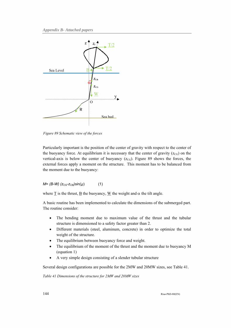
Appendix B- Attached papers
144 Risø-PhD-80(EN)
Particularly important is the position of the center of gravity with respect to the center of the buoyancy force. At equilibrium it is necessary that the center of gravity (zCG) on the vertical-axis is below the center of buoyancy (zCG). Figure 89 shows the forces, the external forces apply a moment on the structure. This moment has to be balanced from the moment due to the buoyancy:
M= (B-W) (zCG-zCB)sin() (1)
where T is the thrust, B the buoyancy, W the weight and the tilt angle.
A basic routine has been implemented to calculate the dimensions of the submerged part. The routine consider:
The bending moment due to maximum value of the thrust and the tubular structure is dimensioned to a safety factor greater than 2.
Different materials (steel, aluminum, concrete) in order to optimize the total weight of the structure.
The equilibrium between buoyancy force and weight.
The equilibrium of the moment of the thrust and the moment due to buoyancy M (equation 1)
A very simple design consisting of a slender tubular structure
Several design configurations are possible for the 2MW and 20MW sizes, see Table 41.
Table 41 Dimensions of the structure for 2MW and 20MW sizes
R
W
B
T/2
O
Sea bed
Sea Level
ZCG
ZCB . .
T/2
y
Figure 89 Schematic view of the forces
z zr

Appendix B- Attached papers
145 Risø-PhD-80(EN)
Size 2MW 20MW
Radius of the rotor structure
(m) 2 3
Radius of the submerged
part (m) 6 6.5
Thickness (m) 0.03 0.03
Total weight (tons) 2300 13000
Rotor length (m) 80 240
Total length (m) 161 345
5.2 Next Development
The next step in the technological development is the implementation of an aeroelastic and hydrodynamic coupled code. At Risø DTU a code has been developed for horizontal-axis floating turbines, HAWC2 [8]. The PhD project is ongoing to implement an aerodynamic subroutine for VAWT to HAWC2 . Indeed the equilibrium and the loads on a floating HAWC have been studied [9,10]. The influence of the rotation of the structure and of the cycling loads of a VAWT rotor is now being investigated.
Another subroutine to add is a subroutine to calculate the friction force around the rotating foundation. Preliminary studies indicate that this drag is insignificant (around 1% of the power). A more detailed analysis is needed, that includes other variables: influence of marine growths, change of roughness, current and waves.
In the meantime some future developments have been planned. In 2010 a kW size prototype will be built and tested in Roskilde fjord. This will be a concept test to verify the feasibility of the concept. A one year friction experiment will explore on friction and marine growths around a rotating cylindrical structure.
Looking forward (2011-2015), also an upscaling phase has been planned. A first demonstration project is planned with a turbine size in the order of 100kW. In the meantime feasibility studies of a MW scale turbine will go on a parallel track.
6. Commercial perspectives
Large scale wind energy systems at highly potent wind resource areas are key candidates for significant contributions to the energy supply. The most potent wind resource areas

Appendix B- Attached papers
146 Risø-PhD-80(EN)
on the earth are deep sea offshore sites, and the potentially most interesting wind energy system for deployment at such sites are floating multi-MW size wind turbines. The primary markets are at deep sea offshore sites along the coasts of for example Norway, France, Spain, the Pacific and Atlantic Ocean (USA) and Asia (China and Japan) and close to big cities. Along with development, optimized floating concepts could be commercialized for places like the North Sea or coastal shallow seas. On the long term exploitation of the wind resources in the "roaring forties" on the southern planet can be made possible with this concept combined with battery or hydrogen tankers that supports energy to coastal cities.
New business opportunities might enter the market in the marine operations and shipping sector, and in the shipyard industry. They will develop sea vessels accordingly with handling, manufacturing and operation of these large wind systems in mind:
Ships with towing capacity and with pultrusion factory on board
Shipping companies might trade electricity with battery ships gathering electricity from remote offshore wind farms.
Floating factories might be developed for very large concepts (support structure for instance made with concrete composites)
The new concept contributes significantly with added value of technology to the wind industry if the concept is developed and demonstrated under real conditions. Within this perspective, the new concept may become an interesting competitor to concepts like HYWIND[1], SWAY[2], BLUEH[3] and NOVA[5], presently being closer to demonstration.
References
1. Hywind Floating wind power production. Alexandra Bech Gjørv Oil & Energy
2006-05-24
2. sway.no
3. www.bluehgroup.com
4. A needed change in orientation. Pierce, WindTech international October 2007
5. www.nova-project.co.uk
6. www.ecopowerusa.com
7. www.selsam.com
8. How 2 HAWC2, The user’s manual, T.J. Larsen and A.M. Hansen. Risø-R-1597, 2008

Appendix B- Attached papers
147 Risø-PhD-80(EN)
9. Responses of Floating Wind Turbines to Wind and Wave Excitation, Master thesis in Ocean Engineering, K. H. Lee, Massachusetts Institute of Technology, 2005
10. Loads Analysis of Floating Offshore Wind Turbine Using Fully Coupled Simulation, Wind power 2007; J.M. Jonkman, M.L. Buhl, Los Angeles, California, 2007
Appendix B- Attached papers
148 Risø-PhD-80(EN)
Proceedings of the ASME 2010 29th International Conference on Ocean, Offshore and Arctic Engineering OMAE2010 June 6-11, 2010, Shanghai, China
OMAE2010-20357 A Novel concept for floating offshore wind turbines: Recent developments in the Concept and invesigation on fluid Interaction with the rotating foundation
Luca Vita Risø DTU
Frederik Zahle Risø DTU
Uwe S. Paulsen Risø DTU
Troels F. Pedersen Risø DTU
Helge A. Madsen Risø DTU
Flemming Rasmussen Risø DTU
Risø National Laboratory for Sustainable Energy
DTU, Technical University of Denmark
Roskilde 4000 Denmark
Appendix B- Attached papers
149 Risø-PhD-80(EN)
ABSTRACT This paper describes the recent developments regarding a new concept for deep sea offshore vertical axis wind turbines. The concept utilizes a cylindrical foundation rotating in the water. The 2D Navier-Stokes solver EllipSys2D has been used to investigate the interaction between the rotating foundation and a water flow stream passing the turbine. Lift and drag forces, and the friction moment on the rotating foundation of the turbine have been computed. The calculations are repeated for different operating conditions of the wind turbine on a range of rotational speeds. The Reynolds number, based on the diameter of the foundation, is 5×10⁶.
Keywords: Vertical Axis Wind Turbine, Floating, Offshore, deep sea, rotating cylinder, lift, friction.
1. Introduction
The fast growth of the wind energy market has increased the strategic importance of offshore wind energy. The European annual report [2] predicts a growth in the European wind energy production from 119 TWh (2007) to 935 TWh (expected in 2030). The electricity production from offshore wind energy is expected to increase from 4 TWh (2007) to 469 TWh (expected in 2030). Thus the share of the offshore production will increase from 3% to 50%. On the other hand, the economic wind energy report from EU [3] (2009) addresses an important cost issue: in average, the cost of offshore wind energy is 2400 Euro/kW versus the 1250 Euro/kW of the on shore (data 2008), with a quite different cost break down in the two cases.
This scenario defines the border lines of a new market, distinct from the ongoing onshore wind energy. If we consider offshore wind energy as a new independent market, it is not reasonable to produce offshore wind energy just moving wind energy technology from onshore out into shallow waters. New specific offshore concepts are needed in order to reduce the cost (to be competitive with the onshore market) and to exploit the considerable offshore wind energy resources.
One of the key challenges is the possibility to optimize wind energy systems for deep water sites with floating wind turbines. This new technology becomes attractive for water deeper than 50 m, and it pushes the limit of the water depth to several hundred meters.
The authors presented in [1] a new concept for floating offshore wind turbines (Figure 90), that is suitable for deep water. The concept has an extremely simple design which simplifies its up-scaling. The main characteristic is that the floating foundation is rotating in the water.
In [1], the most important challenges have been pinpointed, which need to be investigated in order to validate the feasibility of the concept. These challenges consist of: the investigation of the hydrodynamic forces acting on the rotating structure in a water flow stream; the torque absorption at the bottom of the rotor and the dynamic loads on the shaft; the control system; the maintenance strategy for the underwater components.

Appendix B- Attached papers
150 Risø-PhD-80(EN)
Figure 90 Artistic view of the concept.
This paper deals with the hydrodynamic forces generated by a water stream passing the rotating foundation. These forces occur due to the water currents and due to the motion of the foundation. A cylindrical structure rotating in a fluid experiences two forces (lift and drag) and one moment (friction). The two non-dimensional parameters governing the physics of the problem are: the Reynolds number (Re=
Dv/U) and the ratio of peripheral speed and the freestream speed (R/U). The first studies on a rotating cylinder were carried out by Prandt [16]. He found that the
CL (lift coefficient) increased linearly with until an asymptotic value, i.e.
CLMax=4. In the last 50 years many numerical, theoretical and experimental studies have been carried out, as well summarized by Mittal [7] and Padrino[5].
Unfortunately most of the studies are numerical at low Re (<1000) and low . The typical values for our floating foundation are in order of Re=106. The first numerical study was made by Glauert [6], who solved the two dimensional Navier-Stokes equations. Glauert’s results show that the lift increases linearly and indefinitely with
, exceeding the limit of Prandtl. Other studies show different results: Chew [8] confirms in his numerical studies the results of Prandtl; however the experiments by Tokumaru [4] and the numerical model by Mittal [7] show a value of the lift higher than the limit of Prandtl, even if an asymptotic value is observed as well. The value
of when the vortex shedding ceases and the lift tends to and asymptotic value is
called limit L).The value of L depends on Re. For very low Re (Re<160) this
value is a logarithmic function of Re, for Re>1000 it seems to be constant, i.e. L =2 [7].
Some numerical results at higher Re (104<Re<106) are presented by Chang [9]. The stopping of vortex shedding is shown and the lift seems to decrease at high Re. Unfortunately, the numerical simulation at high Re are very limited in time because of convergence problems and it is not possible to predict a fully developed regime.

Appendix B- Attached papers
151 Risø-PhD-80(EN)
The boundary layer around a rotating cylinder is described by Padrino [5] and Wang [11] for Re<1000. The friction torque coefficient is reported and it seems to decrease by the Re number. Another possibility to calculate the friction of a rotating cylinder at high Reynolds numbers is shown in [10] by Theodorsen.
In the present paper the forces and the friction moment on the rotating structure are calculated by numerical simulation, using the code EllipSys2D developed in collaboration between DTU and Risø DTU. The simulation is repeated for different operating conditions of the wind turbine at different rotational speeds. The results
show a steady solution for and the maximum lift coefficient achieved is 10.4
(for
The results are used to calculate the force acting on the structure at different operating conditions and the friction losses in terms of percentage of the nominal power.
2. Concept description The concept consists of a Darrieus rotor whose tower is extended underwater, in order to act as a spar buoy. The whole system is rotating and generates power with a generator placed at the tower bottom and fixed at the anchoring system.
Figure 91 Darrieus rotor, torque arms and mooring system, top-view.
Figure 92 Darrieus rotor, floating foundation and torque arms, trimetric-view.

Appendix B- Attached papers
152 Risø-PhD-80(EN)
Three rigid torque arms connect the generator to the mooring system and absorb the torque (Figure 91 and Figure 92).
Due to its simplicity many solutions are available for the design. Some specific solutions have been selected and they are described below.
ROTOR
A 2 bladed Darrieus rotor has been selected. The choice of 2 blades is to facilitate the installation procedure and to minimize the production costs [12].
BLADES
The blades have a constant geometry along the length. They can be realized in GRP (reinforced glass fibers) by a pultrusion process. Their cost is expected to be comparable to the blades for horizontal axis wind turbines.
SAFETY SYSTEM
Since the whole system is rotating, it is possible to use water brakes as safety system. They consist of drag devices deploying from the rotating foundation in over-speeding conditions (Figure 93).
Figure 93 Water brakes (safety system).
CONTROL SYSTEM
The control system is achieved by controlling the rotational speed of the generator. At cut-out the turbine is stopped by the generator and the safety system.
No yaw system is needed for VAWTs.
GENERATOR
The generator has several functions:
Appendix B- Attached papers
153 Risø-PhD-80(EN)
- To generate power. - To start the turbine, since the VAWTs are not self starting. - To control the system by varying the rotational speed. - To act as a brake in over-speeding condition. - To stop the turbine.
In order to control the turbine, the generator has to be a variable speed generator. Due to its placement in the bottom of the structure, it acts as a counterweight. Therefore the generator has no restrictions due to the weight.
The multi-pole permanent magnet generators seem to fit these prerequisites.
ANCHORING SYSTEM
As mentioned, torque arms are necessary to absorb the torque at the bottom of the structure. The dimension of the anchoring system is the most critical since it has to absorb the reaction forces (torque, thrust and hydrodynamic forces) at the bottom of the structure.
Specific procedures for installation and O&M are suggested as well.
INSTALLATION
Using a two bladed rotor, the turbine and the foundation can be towed to the site by a ship. The structure, without counterweight, can float horizontally in the water. Ballast can be gradually added to tilt up the turbine.
O&M
Moving the counterweight in the bottom of the foundation is possible to tilt up the submerged part for service, in particular build up of marine growths. It is possible to place a lift inside the tubular structure for easy access from the top of the turbine to the submerged part.
3. Sizes and performances The design of the Darrieus rotor and of the rotating foundation are coupled
The design of the underwater part is a compromise between several issues:
- Balancing the forces and the moments due to the weigh, the buoyancy and the aerodynamic thrust. This objective is achieved by varying the volumes of the submerged foundation and the values of the counterweight.
- Reducing the radius and the rotational speed to avoid critical hydrodynamic forces and friction losses
- Reducing the total length, in order to reduce forces and moments and to reduce the production costs.
In Table 42, the dimensions of the concept are shown for 2 MW and 20 MW. The simple concept design facilitates up-scaling.

Appendix B- Attached papers
154 Risø-PhD-80(EN)
Table 42 Dimensions of the rotor and of the rotating foundation, for 2 MW and 20 MW
Size 2MW 20MW
Rotor Diameter (m) 67 120
Rotor Height (m) 75 240
Chord (m) 3.2 11
Torque at rated power (N×m)
1.4×10⁶ 5×10⁷
Thrust at rated power (N)
2.4×10⁵ 2.5×10⁶
Rotational speed at rated power (rpm)
15.0 4.1
Radius of the rotor tower above the water level (m)
2 3
Radius of the submerged part of the tower (m)
2.5 6.5
Total weight (tons) 2300 13000
Total length (m) 160 345
However a full study of a 20 MW machine requires more in depth knowledge of the concept, the different materials and deep water site conditions.
A more detailed investigation has been carried out on the 2MW size.
The solidity of the rotor (=Nc/R), is equal to 0.19. This value is a compromise
between the optimization of the rotor performances (higher values of ) and the
reduction of the cost (0.1 is the optimum value), [12].
The aspect ratio of the rotor, defined as ratio between height and diameter of the rotor, is 1.12. Also this value is a compromise between the optimum, discussed by Paraschivoiu to be around 1.3 [12], and the reduction of the costs, obtained by reducing the height. It is useful to stress that a taller rotor in turn also requires a deeper foundation. This means higher costs in terms of: longer structure, larger forces on the submerged part and larger values of the frictional losses to the nominal power.
Numerical simulations have been performed using a multiple stream tube model, developed at Risø-DTU. The airfoil used for the simulation is a NACA 0018.

Appendix B- Attached papers
155 Risø-PhD-80(EN)
In Figure 94, power coefficient Cp and the power are plotted versus the tip speed
ratio (=R/wsp).
0 2 4 6 8 10
Cp
0,0
0,1
0,2
0,3
0,4
0,5
P [
W]
0,0
5,0e+5
1,0e+6
1,5e+6
2,0e+6
2,5e+6
CpP
Figure 94 Power and Cp versus the tip speed ratio.
In the next charts the thrust and the power versus the wind speed (
Figure 95) are reported, and the power versus the rotational speed (
Figure 96). The turbine has a cut-in wind speed of 5.5 m/s, a cut-out wind speed of 28 m/s and the rated power is achieved at 15m/s, consistent to offshore environment and high wind resources.
At wind speeds higher than 15m/s, the power is kept constant by increasing the rotational speed. This possibility is risky because a negative variation in the wind speed can cause a positive variation of the power. Therefore it would require a very fast and accured rotational speed control system.
An alternative solution could be to keep constant the rotational speed at wind speeds higher than 15m/s. In this case the power would decrease as in Figure 94 and no instability could occur.
On figure 6 and figure 7, four operational points correspond to four rotational speeds. They are representative of four operational conditions of the turbine:
- 5.5rpm (starting of the rotor) - 11rpm (corresponding to the peak of the Cp) - 15rpm (corresponding to the peak of P) - 20rpm (rotor constant power at high wind speed, corresponding to the
maximum value of the thrust) The forces acting on the submerged foundation at these four operating points are analysed. The flow around the cylinder is computed: the lift, the drag and the friction moment are calculated.

Appendix B- Attached papers
156 Risø-PhD-80(EN)
wsp [m/s]
0 5 10 15 20 25 30
P [
W]
-5,0e+5
0,0
5,0e+5
1,0e+6
1,5e+6
2,0e+6
2,5e+6
T [
N]
0
1e+5
2e+5
3e+5
4e+5
5e+5
0
1e+5
2e+5
3e+5
4e+5
5e+5
PowerThrust
Figure 95 Thrust and Power versus the wind speed. The red dots refer to operating points (rotational speeds) and are selected for further investigation.
[rpm]
0 5 10 15 20
P [
W]
-5,0e+5
0,0
5,0e+5
1,0e+6
1,5e+6
2,0e+6
2,5e+6
Figure 96 Power curve versus the rotational speed. The red dots refer to operating points (rotational speeds) and are chosen to investigate the hydrodynamic forces.
4. CFD COMPUTATIONAL TOOL For all computations, the EllipSys2D pressure based incompressible Reynolds averaged Navier-Stokes flow solver written by Michelsen [13,14] and Sørensen[15] is used. The code uses the finite volume method, solving for the primitive variables u, v, w, and p, in general curvilinear coordinates. The variables are stored in a collocated grid arrangement, and odd/even pressure decoupling is avoided using the Rhie-Chow interpolation.
The iterative PISO algorithm is used to advance the solution in time using a second-order accurate scheme. The convective terms are discretized using the Quadratic Upstream Interpolation for Convective Kinematics Scheme, QUICK, and the viscous terms are discretized using central differencing. The momentum equations are solved decoupled from each other using a red/black Gauss-Seidel point solver. To accelerate the convergence of the pressure-correction equation, a multi-grid solution

Appendix B- Attached papers
157 Risø-PhD-80(EN)
strategy is implemented combined with the additive Schwarz method, where each sub-domain is solved for simultaneously. To further accelerate the convergence of the solution, grid and time step sequencing is used.
The simulations were carried out using a combination of steady state and unsteady simulations. Due to the low freestream velocity, convergence was very slow, and as such the unsteady simulations were started from an initial steady state guess. The time step used in the unsteady simulations was set to Δt=0.01 s. Fully turbulent flow was assumed over the cylinder using the k-ω SST turbulence model. The mesh which was used was a curvilinear mesh using an O-type grid with a first cell height corresponding to a y+ of less than two. The outer boundary was placed 100 cylinder diameters away from the cylinder. The rotational speed was prescribed on the cylinder surface to account for the rotation.
5. RESULTS The numerical simulations have been carried out at an inflow velocity of 1m/s corresponding to Re= 5×10⁶.
The calculations are repeated at four operating conditions, corresponding to different
rotational speeds. The speed ratios and the corresponding rotational speeds are listed in Table 5.
Table 43 speed ratios corresponding to the selected rotational speeds
1.4 2.9 3.9 5.2
[rpm] 5.5 11 15 20
Due to the variation of from 1.4 to 5.2) different flow regimes are expected around the cylinder at different operating conditions.
The results and the analysis of the flow regime are reported for the different speed ratios.
=1.4
At the lowest speed ratio the separated shear layer becomes unstable in the wake which gives rise to some unsteadiness in the lift and drag on the cylinder due to beginning vortex shedding (Figure 17). The lift coefficient was found to be equal to 3.99, the CD to 0.180 and the CM to 0.0307.

Appendix B- Attached papers
158 Risø-PhD-80(EN)
Figure 97 Vorticity contours around the cylinder at 1.4, U=1m/s.
=2.9
The increased rotation delays separation of the shear layer which causes the flow to be steady in the wake of the cylinder. An approximately linear increase of lift is
measured compared to 1.4 resulting in a CL of 9.5.
=3.9
This speed ratio is representative of rated power conditions (=15). Due to the relatively high rotational speed, the flow is highly influenced downstream and upstream. The high rotational speed causes the flow to be entirely steady around the cylinder, eliminating vortex shedding which would otherwise be present on a cylinder in this Reynolds number range. This is illustrated in Figure 18 and Figure 19, where the vorticity magnitude and pressure coefficient contours are plotted.
The resulting forces on the cylinder are considerable with a lift coefficient CL of 10.1, corresponding to a total force of 25.2 kN/m, and a drag coefficient CD=-0.016 (40N/m). The drag force changes its direction, respect to the lower rotational speed and it acts as a thrust.
The friction moment coefficient is equal to 0.013, corresponding to a friction moment of 324 Nm/m.
Figure 98 Pressure coefficient contours around the cylinder at 3.9, U=1m/s.
Figure 99 Vorticity contours around the cylinder at 3.9, U=1m/s.

Appendix B- Attached papers
159 Risø-PhD-80(EN)
=5.2
At the highest rotational speed, the flow bears the same characteristics as for 3.9 with a slightly increased CL, the drag is still acting as a thrust and the CM is the double than in the previous conditions.
6. DISCUSSION The force coefficients calculated for the different rotational speeds are summarized in Table 44.
Table 44 Forces and moment coefficients at different
CL CD CM
1.4 (5.5rpm)
3.99 0.180 0.0307
2.9 (11rpm)
9.50 0.0009 0.06914
3.9 (15rpm)
10.1 -0.016 0.12973
5.2 (20rpm)
10.4 -0.043 0.2493
The values of CL are surprisingly close to the values reported by Tukumaru in [4]. Tokumaru compares his experimental data with the experimental data from Prandtl [16 ] and Reid [17]. The data of Tokumaru show a CL around 10.0 at Re 3.8×10³. In the experiment of Reid, CL achieves a value between 9.0 and 10.0 at Re 4.7×10⁴. The data from Prandtl under estimate the CL, but that is probably due to the low ratio of the cylinder span and the diameter used in Prandtl’s experiment. Numerical computations for Re<103 report CL greater than 10 [5,6].
In
Figure 100, the data obtained by using EllipSys2D at Re 5×10⁶ are plotted with the data reported by Tokumaru. The CL seems to be insensitive to the increasing of the
Reynolds number for values of between 3 and 4. At higher values of Tokumaru achieves higher values of CL than EllipSys2D and this can be due to 3D effects.

Appendix B- Attached papers
160 Risø-PhD-80(EN)
0 2 4 6 8 10 12
CL
0
2
4
6
8
10
12
14
16
18
Tokumaru Re=3.8x10³
Reid Re=4.0x10⁴
Reid Re=5.6x10⁴
Prandtl Re=5.2x10⁴
EllipSys2D Re=5.0x10⁶
Figure 100 Values CL from EllipSys2D at Re 5×10⁶(○), from Reid at Re 4×10⁴ (□) and 5.6×10⁴ (☆) [17], from Prandtl at Re 5.2×10⁴ (▲) [16], from Tokumaru at Re 3.8×10³ (◊) [4]. Data from [4].
In Table 45, the lift, the drag and the friction moment are reported for length of unity.
At rated power conditions, a lift of 2.52×10⁴N/m acts on the submerged foundation. The total force, integrated over the whole structure is 2.14×10⁶N, being much larger than the value of the aerodynamic force.
Table 45 Forces and moment per length at different
Lift (N/m) Drag (N/m) Friction moment (N×m/m)
1.4 (5.5rpm)
9950 450 76.5
2.9 (11rpm)
23720 2.2 172.5
3.9 (15rpm)
25148 -41 323.7
5.2 (20rpm)
25860 -106 622
At rated power conditions the friction moment per length corresponds to a power of 508W/m. The total power consumption from friction is 43.2kW, corresponding to a friction to the nominal power ratio of 2.2%. The same analysis has been carried out with the data suggested by Theodorsen in [10]. In his data, Theodorsen suggests to

Appendix B- Attached papers
161 Risø-PhD-80(EN)
compute the friction moment per length unit on revolving cylinders using the
formula MF= CFD42/16, CF is the skin friction factor that Theodorsen calculates with an empirical logarithmical formula. The CF results to be 2.22×10⁻³ at Re 5×10⁶ and MF=644 Nm/m. The ratio of friction to nominal power is 4.3%.
In
Figure 101, the data from Thodorsen and from EllipSys2D are compared at the four rotational speeds.
Both the data seem to follow an exponential fit curve, but the Theodorsen’s formula overestimates the friction moment for higher rotational speeds.
0 1 2 3 4 5 6 7
Po
wer
loss
es to
the
nom
inal
pow
er
0,00
0,05
0,10
0,15
0,20
0,25
Theodorsen formulaData from EllipSys 2D
Figure 101 Power losses to the nominal power versus . The blue line is obtained by using the formula reported in [10] by Theodorsen and the red dots are the values achieved by EllipSys2D.
In Table 8, the forces and the friction moment acting on the turbine at the four operating conditions are summarized (U=1m/s is considered). In all the conditions, the thrust is small compared to the lift force acting on the underwater foundation. The power friction is compared to the power production at the same rotational speed and not to the nominal power. The power friction has a maximum of 5.6% during operational conditions.
Table 46 Forces acting on the turbine, power production and power friction at the four operating conditions
Lift [kN] Thrust [kN]
Friction power [kW]
Power [kW]
Friction /power
1.4 845.7
65.81 3.71 0.00 /
2.9 2016.2
186.85 16.69 1050 0.012
3.9 2137.6
239.65 43.20 1960 0.022
5.2 2198.1 400.00 109.49 1900 0.056

Appendix B- Attached papers
162 Risø-PhD-80(EN)
7. CONCLUSIONS A concept for floating offshore wind turbines has been presented, including the dimensions and the characteristic curves of the rotor. The main challenge for the concept development is the study of the hydrodynamic forces on the rotating foundation. Four operation conditions have been selected and the forces have been investigated for each of them.
The investigations, carried out in EllipSys2D, show force coefficients consistent
with other results at lower Re [4]. At nominal power conditions (at =3.9) a CL of 10.1 is achieved when the solution of the flow appears steady.
Vortex shedding was observed only for the lowest rotational speed (at =1.4).
The force coefficients calculated by numerical simulations are used to calculate the forces acting on the rotating foundation. For rated power conditions
(=3.9,=15rpm) a force of 2.52×10⁴ N/m is achieved. The total force on the submerged foundation is of 2.14×10⁶ N that is almost 10 times larger than the thrust at the same conditions. It has to be stressed that from these studies, the hydrodynamic forces are the most important parameters in the design of the concept. Therefore it is important to know the ocean currents before this concept can be applied.
Further investigations have to concern the variation of the forces in both time and space domain. Indeed the results of this paper concern the forces for a 1D inflow stream at U=1m/s. In steady water conditions, the thrust is the larger force acting on the structure. In a 3D flow, the different sections of the submerged foundation may additionally be loaded with forces in different directions.
The friction moment, acting in the direction opposite to the foundation rotation, is used to calculate the total friction on the foundation, in terms of power losses. At rated power conditions, the friction to nominal power ratio is 2.2%, a higher value (4.3%) was achieved by using the literature [10].
However it is stressed that experimental results would be needed to fully validate the numerical results. Unfortunately, to reproduce the flow regimes investigated in this paper correctly, it would require a quite complex experimental set up. It should reflect the high Re and the high distortion of the flow around the cylinder, which is expected from numerical simulation. Also, the ratio of the cylinder span to the diameter should be correctly reproduced, as described by Tokumaru in his experimental set up and results [4].
NOMENCLATURE
CP= Power coefficient of the rotor
CPMAX= Max value of the power coefficient of the rotor
Appendix B- Attached papers
163 Risø-PhD-80(EN)
CD= Drag coefficient of the cylinder (rotating foundation)
CF= Skin friction coefficient of the cylinder (rotating foundation)
CL= Lift coefficient of the cylinder (rotating foundation)
CLMAX= Maximum value the lift coefficient of the cylinder (rotating foundation)
CM= Friction moment coefficient of the cylinder (rotating foundation)
D= Diameter of the submerged foundation
L= length of the submerged foundation
MF= Friction Moment
N= Number of blades
P= Power of the rotor
PMAX= Max value of the power
R= Radius of the rotor
U= Water stream flow velocity
c= Chord length
p= Pressure
u,v,w= Components of the velocity U
wsp= Wind speed
= speed ratio of peripheral speed and the stream speed
L= speed ratio limit
= Tip speed ratio
= Kinematic viscosity of the water
= Density of the water
= Solidity of the rotor
= Rotational speed of the rotor
REFERENCES
1. Vita L., Paulsen U.S., Pedersen T.P., Madsen H.A., Rasmussen F., (2009). “A Novel Floating Offshore Wind Turbine Concept” EWEC2009, Marseille, France

Appendix B- Attached papers
164 Risø-PhD-80(EN)
2. “Pure Power-Wind Energy Scenarios up to 2030” (2008) European Wind Energy association
3. S. Krohn, P. Morthorst, S.Awerbuch (2009) “The Economics of Wind Energy” European Wind Energy Association
4. P.T. Tokumaru, P.E.Dimotakis (1993) “The lift of a cylinder executing rotary motions in an uniform flow” J. Fluid Mechanics, vol.255
5. J.C. Padrino, D.D. Joseph (2006) “ Numerical study of the steady-state uniform flow past a rotating cylinder“, J. Fluid Mechanics, vol. 557
6. M.B. Glauert (1957) “The flow past a rapidly rotating cylinder” Proceedings of the Royal Society of London, vol.242
7. S. Mittal, B. Kumar (2003) “Flow past a rotating cylinder”, J. Fluid Mechanics, vol.476
8. Y.T. Chew, M. Cheng, S.C. Luo (1995) “A numerical study of flow past a rotating circular cylinder using a hybrid vortex scheme”, J. Fluid Mechanics, vol. 299
9. C.C. Chang, R.L. Chern (1991) “Vortex shedding from an impulsively started rotating and translating circular cylinder”, J. Fluid Mechanics, vol.233
10. T. Theodorsen, A. Regier (1946) “Experiments on drag of revolving disks, cylinders and streamline rods at high speeds”
11. J.Wang, D.D. Joseph “Boundary layer analysis for effect of viscosity on the irrotational flow induced by a rapidly rotating cylinder in a uniform stream”, J. Fluid Mechanics, vol.557
12. I. Paravischivoiu (2002) “Wind Turbine Design, with emphasis on Darrieus concept”, Polytechinc International Pres
13. Michelsen JA (1992) “Basis3D - a Platform for Development of Multiblock PDE Solvers.”, Technical Report AFM 92-05, Technical University of Denmark
14. Michelsen JA (1994) “Block structured Multigrid solution of 2D and 3D elliptic PDE's.” Technical Report AFM 94-06, Technical University of Denmark
15. Sørensen NN (1995) “General Purpose Flow Solver Applied to Flow over Hills.” Risø-R-827-(EN), Risø National Laboratory, Roskilde, Denmark
16. L. Prandtl (1925) Die Naturwissenschaften, vol. 13, pp. 93-108. (English transl: Application of the “Magnus Effect” to the wind propulsion of ships. NACA Tech. Mem. 387, June 1926.)
17. Reid E.G. (1925) “Test of rotating cylinders”, NACA Tech. Note 209

Risø-PhD-80(EN)
Risø DTU is the National Laboratory for Sustainable Energy. Our research focuses on development of energy technologies and systems with minimal effect on climate, and contributes to innovation, education and policy. Risø has large experimental facilities and interdisciplinary research environments, and includes the national centre for nuclear technologies.
Risø DTU National Laboratory for Sustainable Energy Technical University of Denmark Frederiksborgvej 399 PO Box 49 DK-4000 Roskilde Denmark Phone +45 4677 4677 Fax +45 4677 5688 www.risoe.dtu.dk