Offshore Wind Energy Installation and Decommissioning Cost Estimation in the U.S. Outer Continental Shelf Authors Mark J. Kaiser Brian Snyder November 2010 Prepared under MMS Contract M10PC00065 by Energy Research Group, LLC Baton Rouge, Louisiana 70820

ii

iii

DISCLAIMER

This report was prepared under contract between the BOEMRE and Energy Research Group. This report has been technically reviewed by the BOEMRE and approved for publication. Approval does not signify that the contents necessarily reflect the views and policies of the BOEMRE, nor does mention of trade names or commercial products constitute endorsement or recommendation for use.

REPORT AVAILABILITY

A complete copy of this report may be downloaded from the BOEMRE Technology Assessment & Research (TA&R) Program’s website at http://www.mms.gov/tarprojects/. This project is numbered as TA&R project 648.

CITATION

Suggested citation: Kaiser, M.J. and B. Snyder 2011. Offshore Wind Energy Installation and Decommissioning

Cost Estimation in the U.S. Outer Continental Shelf. U.S. Dept. of the Interior, Bureau of Ocean Energy Management, Regulation and Enforcement, Herndon, VA. TA&R study 648. 340 pp.

ACKNOWLEDGMENTS The authors wish to thank the Bureau of Ocean Energy Management, Enforcement and Regulation Technology Assessment and Research Branch for funding this study and Lori Medley, Greg Adams, and Bob Mense for critical and insightful comments associated with the work.

ACRONYMS AWC: Atlantic Wind Connection BOEMRE: Bureau of Ocean Energy Management Regulation and Enforcement CBP: Customs and Boarder Protection CFR: Code of Federal Regulations COP: Construction and operation plan CZMA: Coastal Zone Management Act EIS: Environmental impact statement EPACT: Energy Policy Act of 2005 FERC: Federal Energy Regulatory Commission GAP: General activities plan GOM: Gulf of Mexico GSOE: Garden State Offshore Energy HVAC/HVDC: High voltage alternating current/high voltage direct current MARAD: Maritime Administration NEPA: National Environmental Policy Act OCS: Outer continental shelf OSV: Offshore supply vessel OWEZ: Offshore Windfarm Egmond aan Zee PPA: Power purchase agreement REC: Renewable energy credit RPS: Renewable portfolio standard SAP: Site assessment plan SPIV: Self-propelled installation vessel

v

ABSTRACT

Offshore wind power shows promise as a means of carbon neutral electrical generation. In the U.S., offshore wind is expected to commence development between 2015-2020 and will occur primarily in federal waters administered by the Bureau of Ocean Energy Management Regulation and Enforcement (BOEMRE). In order to protect the public interest, BOEMRE is required to ensure that adequate financial assurance exists for wind farm decommissioning in the case the operator defaults or is unable to perform according to the terms of the lease instrument. Consequently, BOEMRE requires information on the expected costs of offshore wind decommissioning. In this report we develop estimates of offshore wind installation and decommissioning costs using a bottom-up engineering based approach and compare with total capital cost and installation cost estimates generated through a reference class approach. We find that installation costs are typically 5 to 15% of overall capital costs and that decommissioning costs are roughly half of installation costs, or roughly 100,000 to 160,000 $/MW. Decommissioning costs and financial assurance depends on the methods developed for decommissioning and regulations concerning the circumstances under which components may be left in place.

vi

vii

TABLE OF CONTENTS

Page

ABSTRACT v 

TABLE OF CONTENTS vii 

LIST OF FIGURES xv 

LIST OF TABLES xix 

EXECUTIVE SUMMARY 1 

1.  OFFSHORE WIND DEVELOPMENT STATUS 4 1.1 Offshore Wind in Europe ......................................................................................................4 1.2 Offshore Wind in the U.S......................................................................................................8 

1.2.1 Cape Wind..................................................................................................................12 1.2.2 Coastal Point Energy-Galveston ................................................................................13 1.2.3 Bluewater Wind-Delaware.........................................................................................14 1.2.4 Deepwater-Rhode Island ............................................................................................15 1.2.5 Garden State Offshore Energy ...................................................................................15 

1.3 Factors Impacting U.S. Development .................................................................................15 1.4 Atlantic Wind Connection...................................................................................................16 

2. OFFSHORE WIND ENERGY SYSTEM COMPONENTS 18 2.1 Meteorological Systems ......................................................................................................18 2.2 Support System ...................................................................................................................19 

2.2.1 Foundation..................................................................................................................19 2.2.2 Transition Piece..........................................................................................................25 2.2.3 Scour Protection .........................................................................................................26 

2.3 Wind Turbine ......................................................................................................................27 2.4 Electricity Collection and Transmission .............................................................................28 2.5 Offshore Substation.............................................................................................................31 2.6 Commissioning....................................................................................................................32 

3. STAGES OF OFFSHORE DEVELOPMENT 33 3.1 Project Location ..................................................................................................................33 

3.1.1 Baseline ......................................................................................................................33 3.1.2 State Waters................................................................................................................33 3.1.3 Outer Continental Shelf..............................................................................................33 

3.2 Development Process ..........................................................................................................33 3.2.1 Lease Acquisition.......................................................................................................33 3.2.2 Assessment .................................................................................................................34 3.2.3 Design.........................................................................................................................34 3.2.4 Construction ...............................................................................................................34 3.2.5 Commissioning...........................................................................................................35 

3.3 Texas Offshore Wind Lease Terms and Conditions ...........................................................35 3.3.1 General Conditions.....................................................................................................35 3.3.2 Galveston Island Lease Terms ...................................................................................38 

viii

TABLE OF CONTENTS (continued)

Page

3.4 Energy Policy Act of 2005 ..................................................................................................40 3.5 Federal Offshore Wind Lease Terms and Conditions.........................................................40 

3.5.1 Types of Access Rights ..............................................................................................40 3.5.2 Auction Method..........................................................................................................41 3.5.3 Leasing Process ..........................................................................................................42 3.5.4 Lease Terms ...............................................................................................................43 3.5.5 Development Process .................................................................................................44 3.5.6 Project Plans...............................................................................................................44 3.5.7 Decommissioning.......................................................................................................44 

4. OFFSHORE PROJECT CHARACTERISTICS 46 4.1 Infrastructure .......................................................................................................................46 

4.1.1 Design Requirements are Site-Specific and Multi-Dimensional ...............................46 4.1.2 Configuration is Dictated by Prevailing Wind Directions and Aesthetic Appeal......47 4.1.3 System Capacities Reflect Farm Purpose...................................................................48 4.1.4 Turbine Selection Has Broad Impacts on System Design..........................................51 4.1.5 Physical and Engineering Laws Induce System-Level Homogeneity .......................51 4.1.6 Cost Comparisons are Facilitated by System Homogeneity ......................................51 

4.2 Markets................................................................................................................................52 4.2.1 Tradeoffs in Vessel Selection and Availability..........................................................52 4.2.2 Installation Vessel Market Transparency is Poor.......................................................52 4.2.3 Varying Levels of Competition..................................................................................52 4.2.4 Learning Curve Uncertainty.......................................................................................53 4.2.5 U.S. Project Economics and Financing Strategies .....................................................54 

4.3 Contracts..............................................................................................................................55 4.3.1 Construction Contracts Define Cost Categories.........................................................55 4.3.2 Risk Allocation and Cost............................................................................................56 4.3.3 U.S. Offshore Wind Will Likely Be Developed Using Multi-Contracting................58 

4.4 Data Limitations..................................................................................................................59 4.4.1 Small Samples and Diverse Project Characteristics...................................................59 4.4.2 Small Samples Also Limit Analytic Techniques .......................................................59 4.4.3 No U.S. Projects are Under Construction ..................................................................59 4.4.4 European Markets Differ in Fundamental Ways from U.S. Market ..........................59 

4.5 Cost......................................................................................................................................60 4.5.1 Vessel Dayrates are Market-Driven and Dynamic.....................................................60 4.5.2 Impact of Catastrophic Failures .................................................................................60 4.5.3 Port Facility and Location Impact Cost......................................................................60 4.5.4 Weather Risk Is Common in all Offshore Construction ............................................60 4.5.5 Public-Private Interface Impacts Cost Structure ........................................................61 4.5.6 All Cost Estimates are Uncertain ...............................................................................63 

4.6 Decommissioning................................................................................................................63 4.6.1 Decommissioning Timing is Defined by Regulatory Requirements .........................63 4.6.2 Each Decommissioning Project Is Unique.................................................................63 

ix

TABLE OF CONTENTS (continued)

Page

4.6.3 Decommissioning Operations Are Low-Tech and Routine .......................................64 4.6.4 Learning Opportunities Will Develop........................................................................64 

4.7 Exposure and Liability ........................................................................................................64 4.7.1 Joint and Several Liabilities .......................................................................................64 4.7.2 Each Lease Represents a Different Level of Decommissioning Risk........................64 4.7.3 Bonding Protects the Public Interest ..........................................................................64 4.7.4 Exposure Limits Vary With a Number of Factors .....................................................65 4.7.5 U.S. Government is the Party of Last Resort .............................................................65 4.7.6 Bonding Cannot Provide Complete Protection from Noncompliance Risk...............65 4.7.7 Financial Failures in Offshore Wind May Be Less of a Threat .................................65 4.7.8 All Bonding Procedures Have Limitations and Constraints ......................................65 

5. INSTALLATION STRATEGIES AND OPTIONS 67 5.1 Foundation Installation........................................................................................................67 

5.1.1 Monopiles...................................................................................................................67 5.1.2 Jackets and Tripods ....................................................................................................70 5.1.3 Factors Impacting Installation....................................................................................70 5.1.4 U.S. Foundation Installation.......................................................................................71 

5.2 Turbine Installation .............................................................................................................71 5.2.1 Transport ....................................................................................................................71 5.2.2 Installation..................................................................................................................72 5.2.3 Factors Impacting Installation....................................................................................76 5.2.4 U.S. Turbine Installation ............................................................................................76 

5.3 Cable Installation.................................................................................................................76 5.3.1 Inner-Array Cable ......................................................................................................78 5.3.2 Export Cable...............................................................................................................78 5.3.3 Factors Impacting Installation....................................................................................80 5.3.4 U.S. Cable Installation ...............................................................................................80 

5.4 Substation Installation .........................................................................................................80 5.5 European Installation Time Statistics..................................................................................81 

5.5.1 Data Source ................................................................................................................81 5.5.2 Foundation..................................................................................................................81 5.5.3 Turbine .......................................................................................................................83 5.5.4 Cable...........................................................................................................................85 5.5.5 Substation ...................................................................................................................86 5.5.6 Reference Class Statistics...........................................................................................87 

6. INSTALLATION AND VESSEL SPREAD REQUIREMENTS 88 6.1 Vessel Categorization..........................................................................................................88 

6.1.1 Main Installation Vessels ...........................................................................................88 6.1.2 Cable-Laying Vessels.................................................................................................91 6.1.3 Vessel Spreads............................................................................................................92 

6.2 Factors Impacting Vessel Selection ....................................................................................94 6.2.1 Foundation..................................................................................................................94 

x

TABLE OF CONTENTS (continued)

Page

6.2.2 Turbine .......................................................................................................................94 6.2.3 Cable...........................................................................................................................95 6.2.4 Substation ...................................................................................................................96 

6.3 Support Spread Size and Composition................................................................................96 6.3.1 Foundations ................................................................................................................96 6.3.2 Turbines......................................................................................................................96 6.3.3 Cable...........................................................................................................................97 6.3.4 Example European Spreads........................................................................................97 6.3.5 Potential U.S. Spreads................................................................................................99 

6.4 U.S. Vessel Procurement.....................................................................................................99 6.4.1 Jones Act ....................................................................................................................99 6.4.2 U.S. Fleet Circa 2010 ...............................................................................................101 6.4.3 Newbuilding.............................................................................................................102 

7. MODELLING INSTALLATION VESSEL DAYRATES 105 7.1 European Installation Vessel Costs ...................................................................................105 7.2 Gulf of Mexico Market Trends .........................................................................................106 

7.2.1 Liftboat Dayrates......................................................................................................106 7.2.2 Jackup Rig Dayrates.................................................................................................106 7.2.3 OSV Dayrates...........................................................................................................108 7.2.4 Newbuild Cost..........................................................................................................108 

7.3 Dayrate Components .........................................................................................................109 7.3.1 Operating Expenses..................................................................................................109 7.3.2 Returns on Investment..............................................................................................110 7.3.3 Finance Costs ...........................................................................................................110 7.3.4 Dayrate .....................................................................................................................111 

7.4 Dayrates as a Proportion of Newbuild Costs ....................................................................112 7.5 Newbuild Program ............................................................................................................114 7.6 Dayrate Estimation in the U.S...........................................................................................116 

7.6.1 Limitations ...............................................................................................................116 7.6.2 Assumptions .............................................................................................................117 7.6.3 Results ......................................................................................................................117 

7.7 Mobilization Costs ............................................................................................................118 7.7.1 Tug Transport...........................................................................................................118 7.7.2 Self-Propelled Transport ..........................................................................................119 7.7.3 Heavy-lift Vessel Transport .....................................................................................119 7.7.4 Example....................................................................................................................120 

7.8 Total Vessel Costs.............................................................................................................122 7.9 Theoretical Model Development.......................................................................................124 

7.9.1 Leasing Dayrates ......................................................................................................124 7.9.2 Newbuilding Dayrate ...............................................................................................125 

8. INSTALLATION COST ESTIMATION – REFERENCE CLASS APPROACH 127 8.1 Cost Categories .................................................................................................................127 

xi

TABLE OF CONTENTS (continued)

Page

8.1.1 Capital and Operating Expenditures ........................................................................127 8.1.2 Capital Cost Categories............................................................................................127 

8.2 Comparative Method.........................................................................................................127 8.3 Source Data .......................................................................................................................128 

8.3.1 Sample Set................................................................................................................128 8.3.2 Exclusion..................................................................................................................128 8.3.3 Reference Class ........................................................................................................128 8.3.4 Adjustment ...............................................................................................................129 8.3.5 Normalization...........................................................................................................134 

8.4 Capital Expenditures .........................................................................................................134 8.4.1 Summary Statistics...................................................................................................134 8.4.2 Time Trends .............................................................................................................134 8.4.3 Economies of Scale ..................................................................................................136 8.4.4 Regression Models ...................................................................................................137 

8.5 Installation Cost Estimation ..............................................................................................142 8.5.1 Model Assumption ...................................................................................................142 8.5.2 Model Results...........................................................................................................145 8.5.3 Uncertainty Bounds..................................................................................................145 

8.6 Model Limitations .............................................................................................................147 8.6.1 Sources of Error and Bias.........................................................................................147 8.6.2 Reference Class Constraints.....................................................................................148 

9. INSTALLATION COST ESTIMATION – ENGINEERING APPROACH 150 9.1 System Description ...........................................................................................................150 

9.1.1 User Data..................................................................................................................150 9.1.2 System Data..............................................................................................................150 9.1.3 Model Output ...........................................................................................................150 

9.2 User Input..........................................................................................................................151 9.2.1 Project Characteristics..............................................................................................151 9.2.2 Vessel Selection .......................................................................................................152 9.2.3 Installation Strategy..................................................................................................152 9.2.4 Adjustment Factor ....................................................................................................153 

9.3 System Data.......................................................................................................................153 9.3.1 Vessel Specification .................................................................................................153 9.3.2 Expected Time..........................................................................................................153 9.3.3 Expected Dayrate .....................................................................................................154 

9.4 Installation Stage Computations........................................................................................154 9.4.1 Foundation and Turbine Installation ........................................................................154 9.4.2 Cable Installation......................................................................................................157 9.4.3 Substation Installation ..............................................................................................162 9.4.4 Scour Protection .......................................................................................................162 9.4.5 Mobilization .............................................................................................................162 

9.5 Model Parameterization ....................................................................................................162 

xii

TABLE OF CONTENTS (continued)

Page

9.5.1 Vessel Data...............................................................................................................162 9.5.2 Foundations ..............................................................................................................163 9.5.3 Turbines....................................................................................................................164 9.5.4 Cables .......................................................................................................................165 9.5.5 Substation .................................................................................................................165 9.5.6 Scour Protection .......................................................................................................166 9.5.7 Mobilization .............................................................................................................166 

9.6 Parameter Verification ......................................................................................................166 9.6.1 Temporal Parameters................................................................................................166 9.6.2 Output Costs.............................................................................................................168 

9.7 Hypothetical 300 MW Windfarm .....................................................................................169 9.7.1 Component Costs .....................................................................................................169 9.7.2 Total Costs................................................................................................................170 9.7.3 Sensitivity Analysis..................................................................................................171 

9.8 U.S. Proposed Projects ......................................................................................................173 9.8.1 Cape Wind - Massachusetts .....................................................................................174 9.8.2 Bluewater Wind - Delaware.....................................................................................175 9.8.3 Coastal Point - Galveston.........................................................................................176 

9.9 Model Limitations .............................................................................................................176 

10. STAGES OF DECOMMISSIONING 178 10.1 Regulatory Requirements................................................................................................178 10.2 Decommissioning Bonds.................................................................................................178 10.3 Financial Instruments ......................................................................................................179 10.4 Stages of Offshore Wind Decommissioning...................................................................179 

10.4.1 Project Management and Engineering ...................................................................179 10.4.2 Turbine Removal....................................................................................................180 10.4.3 Foundation and Transition Piece Removal ............................................................182 10.4.4 Met Tower and Substation Platform Removal.......................................................184 10.4.5 Cable Removal .......................................................................................................185 10.4.6 Scour Protection .....................................................................................................185 10.4.7 Site Clearance and Verification..............................................................................185 10.4.8 Material Disposal ...................................................................................................186 

11. WEIGHT ALGORITHMS 188 11.1 Tubular Weight Algorithm..............................................................................................188 11.2 Foundations .....................................................................................................................189 

11.2.1 Monopile ................................................................................................................190 11.2.2 Transition Piece......................................................................................................191 11.2.3 Grout.......................................................................................................................192 

11.3 Tower and Turbine ..........................................................................................................194 11.3.1 Tower .....................................................................................................................194 11.3.2 Turbine ...................................................................................................................194 

11.4 Cable................................................................................................................................195 

xiii

TABLE OF CONTENTS (continued)

Page

11.5 Substation ........................................................................................................................196 

12. DECOMMISSIONING COST ESTIMATION 197 12.1 Decommissioning Stages ................................................................................................197 12.2 Turbine Removal.............................................................................................................197 

12.2.1 Input .......................................................................................................................198 12.2.2 Self-Transport Model .............................................................................................198 12.2.3 Barge Model...........................................................................................................199 12.2.4 Unconventional Model...........................................................................................200 12.2.5 Parameterization.....................................................................................................200 12.2.6 Example..................................................................................................................202 

12.3 Foundation Removal .......................................................................................................202 12.3.1 Input .......................................................................................................................203 12.3.2 Single-Vessel..........................................................................................................203 12.3.3 OSV Support ..........................................................................................................204 12.3.4 Parameterization.....................................................................................................204 12.3.5 Example..................................................................................................................205 

12.4 Cable................................................................................................................................206 12.4.1 Parameterization.....................................................................................................206 12.4.2 Example..................................................................................................................206 

12.5 Substation and Met Tower ..............................................................................................207 12.6 Scour Protection ..............................................................................................................208 12.7 Site Clearance..................................................................................................................208 

12.7.1 Per-Turbine.............................................................................................................208 12.7.2 Whole Farm............................................................................................................208 12.7.3 Example..................................................................................................................209 

12.8 Material Disposal Costs ..................................................................................................209 12.8.1 Processing Costs.....................................................................................................210 12.8.2 Scrap Value ............................................................................................................210 12.8.3 Landfill Cost...........................................................................................................211 12.8.4 Transport Costs ......................................................................................................211 12.8.5 Reefing ...................................................................................................................211 12.8.6 Example..................................................................................................................212 

12.9 Cape Wind Decommissioning Scenarios ........................................................................212 12.10 Decommissioning Costs at Proposed Offshore Wind Farms ........................................212 12.11 Discussion .....................................................................................................................215 

12.11.1 Proposed U.S. Wind Farms Bonding Requirements ............................................215 12.11.2 Limitations ...........................................................................................................216 

REFERENCES 217 

xiv

xv

LIST OF FIGURES

Page Figure 1.1. Wind Farms over 100 MW Online and Under Construction - October 2010 .............. 4 Figure 1.2. Capacity of European Offshore Wind Farms, Online and Under Construction as of

October 2010................................................................................................................... 5 Figure 1.3. Number of Offshore Wind Farms Built per Year and Average Capacity of New

Farms Greater than 100 MW. ......................................................................................... 5 Figure 1.4. Offshore Wind Capacity Additions and Cumulative Capacity. .................................. 6 Figure 1.5. Offshore Wind Farms Planned for the German Sector of the North Sea .................... 7 Figure 1.6. Round 1 (Yellow) and 2 (Red) Wind Farms in the Thames Estuary, UK................... 8 Figure 1.7. Proposed U.S. Offshore Wind Projects ....................................................................... 8 Figure 1.8. BOEMRE Planning Areas......................................................................................... 11 Figure 1.9. Proposed Cape Wind Turbine and Cable Array ........................................................ 12 Figure 1.10. Location of Coastal Point Leases ............................................................................. 14 Figure 1.11. Proposed Garden State Offshore Energy Project ..................................................... 16 Figure 1.12. Proposed Atlantic Wind Connection and Hypothetical Wind Farms....................... 17 Figure 2.1. Cape Wind (Left) and Coastal Point Energy Meteorological Towers ...................... 18 Figure 2.2. Components of a Monopile Foundation .................................................................... 20 Figure 2.3. Components of a Tripod Foundation......................................................................... 21 Figure 2.4. The Taklift 4 Placing a Tripod Foundation at Alpha Ventus .................................... 21 Figure 2.5. Components of a Jacket Foundation.......................................................................... 22 Figure 2.6. A Jacket Structure Supports the Substation at Alpha Ventus.................................... 23 Figure 2.7. Components of a Gravity Foundation ....................................................................... 24 Figure 2.8. The Eide Barge 5 Lifting a Gravity Foundation at Nysted ....................................... 25 Figure 2.9. The Hywind Turbine and Support Structure ............................................................. 25 Figure 2.10. The Hywind Turbine being Towed Offshore ........................................................... 25 Figure 2.11. Transition Piece at Horns Rev II .............................................................................. 26 Figure 2.12. An Assembled Rotor Being Lifted onto a Nacelle at Nysted................................... 27 Figure 2.13. Diagram of a Nacelle................................................................................................ 29 Figure 2.14. Inside of a Nacelle and Relative Size ....................................................................... 29 Figure 2.15. Layout of Lillgrund .................................................................................................. 30 Figure 2.16. Layout of Middelgrunden......................................................................................... 31 Figure 2.17. Substation Being Lifted onto Monopile at Gunfleet Sands...................................... 32 Figure 4.1. Forces Acting on an Offshore Wind Turbine ............................................................. 46 Figure 4.2. Layout of the Horns Rev Wind Farm......................................................................... 47 Figure 4.3. Layout of Scroby Sands Wind Farm .......................................................................... 48 Figure 4.4. Layout of Middelgrunden........................................................................................... 48 Figure 4.5. Layout Schematics of Selected Offshore Wind Farms............................................... 49 Figure 4.6. Offshore Wind Farm Capacity Installation by Year................................................... 50 Figure 4.7. Number and Total Capacity of Wind Farms by Size Class........................................ 50 Figure 4.8. Relationship between Inner-Array Cable Length and Farm Capacity and Farm Area

and Number of Turbines ..............................................................................................52 Figure 4.9. Self-Propelled Installation Vessel and Jack-Up Barge Tradeoffs .............................. 53

xvi

Figure 4.10. Supply and Demand Factors Influencing Installation Vessel Dayrates ................... 54

LIST OF FIGURES (continued)

Page

Figure 4.11. Hypothetical Learning Curves for Offshore Wind, and Actual Placement of the European Market......................................................................................................... 54

Figure 4.12. Scroby Sands EPC Contract Structure ..................................................................... 57 Figure 4.13. Nysted Multi-Contract Structure .............................................................................. 58 Figure 4.14. Activities at Port Staging Areas ............................................................................... 61 Figure 4.15. Average June (Top), January (Middle) and Annual Wind Speeds........................... 62 Figure 5.1. Monopile upending frame .......................................................................................... 68 Figure 5.2. Hammer Placed on the Top of a Monopile Before Driving ....................................... 68 Figure 5.3. Diagram of a Monopile Foundation Driven into the Seabed. .................................... 68 Figure 5.4. Transition Piece Being Placed over Monopile. .......................................................... 69 Figure 5.5. The Taklift 4 Placing a Tripod Foundation at Alpha Ventus ..................................... 69 Figure 5.6. Jacket and Transition Piece at Beatrice ...................................................................... 70 Figure 5.7. Diagrammatic Representation of Installation Methods.............................................. 72 Figure 5.8. Installation of a Single Blade at Lynn and Inner Dowsing ........................................ 73 Figure 5.9. Lifting a Fully Assembled Tower onto a Transition Piece at Rhyl Flats ................... 74 Figure 5.10. Installation of an Assembled Rotor at Alpha Ventus ............................................... 74 Figure 5.11. Nacelle and Blades in the Bunny Ear Configuration at Kentish Flats ..................... 75 Figure 5.12. The Sea Energy Leaving Port with Two 55 m Towers, Two Bunny-Eared Nacelles

and Two Additional Blades .......................................................................................... 75 Figure 5.13. The Rambiz Installing a Fully Assembled Turbine at Beatrice................................ 75 Figure 5.14. Tracked ROV Operated by the MV Resolution ........................................................ 77 Figure 5.15. A J Tube Being Installed on a Transition Piece ....................................................... 78 Figure 5.16. Horizontal Directional Drilling at OWEZ................................................................ 79 Figure 5.17. The Barge UR101 Beached at Lynn and Inner Dowsing ........................................ 79 Figure 6.1. The KS Titan II Liftboat............................................................................................. 90 Figure 6.2. The Sea Jack under Tow ............................................................................................ 90 Figure 6.3. The JB 114, a MSC SEA 2000 Jackup Barge ............................................................ 90 Figure 6.4. The MV Resolution Working at Barrow..................................................................... 90 Figure 6.5. The Heavy Lift Vessel Rambiz Installing a Turbine at the Beatrice Project.............. 91 Figure 6.6. The Eide 28, an Export Cable Laying Vessel............................................................. 91 Figure 6.7. The Nico, a Modified Offshore Supply Vessel Installing Inner-Array Cable............ 92 Figure 6.8. The Polar Prince, another Cable Laying Vessel........................................................ 92 Figure 6.9. A Rigid Hull Inflatable Boat Used for Personnel Transfer and Utility Work at

Gunfleet Sands .............................................................................................................. 93 Figure 6.10. The Forth Jouster, a 26 m Multicat.......................................................................... 93 Figure 6.11. Diagram of Factors Affecting Lift Height and Capacity.......................................... 95 Figure 6.12. The Spread at Thanet Windfarm by Week ............................................................... 97 Figure 6.13. The Spread at Gunfleet Sands Offshore Wind Farm by Week ................................ 98 Figure 7.1. Average Large Liftboat Dayrates in the Gulf of Mexico ......................................... 106 Figure 7.2. Average Jackup Dayrates in the Gulf of Mexico ..................................................... 107

xvii

Figure 7.3. Average OSV dayrates in the Gulf of Mexico ......................................................... 107 Figure 7.4. Average Newbuild Costs of 300 Foot Water Depth Jack-Up Drilling Rig.............. 108  

LIST OF FIGURES (continued)

Page

Figure 7.5. Shipbuilding Price and Earnings Cost Indices ........................................................ 109 Figure 7.6. Hypothetical Mobilization Locations ...................................................................... 120 Figure 8.1. Diagrammatic Depiction of Alternative Methods of Adjusting Costs for a

Hypothetical €500 Million Wind Farm Built in 2000 ................................................ 131 Figure 8.2. Offshore Wind Farm Capital Expenditure and Time of Contract for Total Sample.

Capacity Size in MW Expressed in Bubble Form. ..................................................... 136 Figure 8.3. Relationship Between Installed Capacity and Normalized Capital Expenditures.... 138 Figure 8.4. Relationship Between Water Depth and Normalized Capital Expenditures ............ 138 Figure 8.5. Relationship Between Distance to Shore and Normalized Capital Expenditures .... 141 Figure 8.6. Relationship Between European CRU Steel Index and Normalized Capital

Expenditures ............................................................................................................... 141 Figure 8.7. Relationship Between Capacity and Capital Expenditures ...................................... 142 Figure 9.1. User-Specified Properties and the Project Parameters They Influence.................... 151 Figure 9.2. Illustration of Self-Transport and Barge Models...................................................... 155 Figure 9.3. Sensitivity of the Self-Transport Model to Changes in Capacity, Distance to Port . 172 Figure 9.4. Sensitivity of the Self-Transport Model to Changes in Turbine Capacity ............... 172 Figure 9.5. Sensitivity of the Self-Transport Model to Changes in Dayrate, Installation Time. 172 Figure 9.6. Installation Time and Cost Range for High and Low Spread Requirements ........... 173 Figure 10.1. Traditional Offshore Turbine Decommissioning Options and an Alternative ....... 181 Figure 10.2. Proposed Alternative Turbine Removal Method.................................................... 182 Figure 10.3. Foundation Removal - External Cut....................................................................... 183 Figure 10.4. Foundation Removal - Internal Cut........................................................................ 183 Figure 11.1. Scale of Windfarm Tubular Components............................................................... 189 Figure 11.2. Components of a Wind Turbine Foundation .......................................................... 190 Figure 11.3. Transition Piece Height Estimation........................................................................ 191 Figure 11.4. Grout Weight Estimation........................................................................................ 193 Figure 12.1. Traditional Turbine Removal Cost at Cape Wind by Assumed Discount Factor .. 203 Figure 12.2. U.S. Heavy Metal Steel Scrap Price....................................................................... 211 

xviii

xix

LIST OF TABLES

Page Table 1.1. Offshore Wind Capacity by Nation – October 2010 ..................................................... 7 Table 1.2. Proposed U.S. Offshore Wind Farms and Development Status – October 2010 .......... 9 Table 2.1. Estimated Distribution of Foundation Types of Offshore Wind Farms ...................... 20 Table 2.2. Weights of Commonly Used Offshore Turbines ......................................................... 27 Table 3.1. Lease Terms for Galveston Island Wind Farm............................................................ 39 Table 3.2. BOEMRE Auction Methods........................................................................................ 41 Table 3.3. Frequency of NEPA/CZMA Reviews Based on Instrument Held .............................. 42 Table 3.4. Commercial Lease Cash Flows.................................................................................... 43 Table 4.1. Turbines Used in Offshore Wind Farms...................................................................... 51 Table 4.2. Offshore Wind Developers in Europe and Potential Developers in the U.S. .............. 55 Table 4.3. Contract Types by Windfarm and Year of Construction............................................. 56 Table 5.1. Number of Offshore Lifts and Approximate Weights for Alternative Turbine

Installation Methods and Turbines........................................................................................ 76 Table 5.2. Sources of Information on Installation Activities at Select Offshore Wind Farms ..... 81 Table 5.3. Offshore Wind Farm Installation Requirements – Foundations.................................. 82 Table 5.4. Rate of Foundation Installation by Number of Foundations in Boat Days per

Foundation ............................................................................................................................ 83 Table 5.5. Offshore Wind Farm Installation Requirements – Turbines ....................................... 83 Table 5.6. Rate of Turbine Installation by Installation Method in Boat Days per Turbine .......... 84 Table 5.7. Rate of Turbine Installation by Number of Turbines in Boat Days per Turbine......... 84 Table 5.8. Rate of Turbine Installation by Installation Method and Number of Turbines in Boat

Days per Turbine................................................................................................................... 84 Table 5.9. Offshore Wind Farm Installation Requirements – Cables........................................... 85 Table 5.10. Rate of Cable Installation by Cable Distance in km/Day .......................................... 86 Table 5.11. Export Cable Installation Time by Voltage and Distance ......................................... 86 Table 5.12. Average Estimated Times Required by Installation Phase and Development Size... 87 Table 5.13. Summary of Time Estimates for Installation of Wind Farm Components in Boat

Days per Unit ........................................................................................................................ 87 Table 6.1. Vessels Used in Offshore Wind Farm Construction in Europe ................................... 89 Table 6.2. Vessel Capabilities by Work Type .............................................................................. 94 Table 6.3. Estimated Potential Spreads by Vessel Type and Activity.......................................... 96 Table 6.4. Average Number of Support Vessels Required per Construction Vessel at Thanet and

Gunfleet Sands ...................................................................................................................... 98 Table 6.5. Elevating Vessels Active in the U.S. and/or with U.S. Flags Capable of Offshore

Wind Farm Construction..................................................................................................... 101 Table 6.6. Non-Elevating Vessels Active in the U.S. or with a U.S. Flag Capable of Offshore

Wind Farm Construction..................................................................................................... 102 Table 6.7. Specification of Newbuild Designs ........................................................................... 103 Table 6.8. U.S. Commercial Shipbuilders Capable of Building Turbine Installation Vessels ... 104 Table 7.1 Operating Expenses for Selected Commercial Vessels in the Gulf of Mexico (2009-

2010) ................................................................................................................................... 110

xx

Table 7.2. Dayrates Estimated for Alternative Cost Scenarios................................................... 111 Table 7.3. Regression Analysis of the Lease Dayrate Model ..................................................... 112

LIST OF TABLES (continued)

Page

Table 7.4. Turbine Installation Vessel Dayrates as a Percentage of Capital Costs .................... 113 Table 7.5. Estimated Dayrates for a Developer Using Their Own Newbuilt Vessel, Sold at the

Conclusion of the Project.................................................................................................... 116 Table 7.6. Regression Analysis of Costs to a Developer of Newbuilding their own Vessel...... 116 Table 7.7. The Range of Vessel Dayrates under Alternative Assumptions and Models ............ 118 Table 7.8. Mobilization Distances Between Alternative Locations ........................................... 121 Table 7.9. Ranges of Mobilization Costs by Method of Mobilization ....................................... 121 Table 7.10. Total Vessel Cost for a One-Year Installation Project ............................................ 123 Table 8.1. Wind Farms Included in the Sample and Reference Class........................................ 129 Table 8.2. Impact of Alternative Methods for Adjusting Costs.................................................. 131 Table 8.3. Inflation and Exchange Rate Cost Normalization Assumptions ............................... 132 Table 8.4. Capital Costs of Offshore Windfarms in the Total Sample ....................................... 133 Table 8.5. Comparison of Normalized Capital Costs by Source (Million $/MW)..................... 135 Table 8.6. Offshore Wind Farm CAPEX by Year of Initial Operation ...................................... 136 Table 8.7. Average CAPEX by Installed Capacity..................................................................... 136 Table 8.8. Offshore Wind Farm CAPEX by Capacity and Year Online (Million $/MW)......... 137 Table 8.9. Summary of Capital Cost Regression Model ............................................................ 140 Table 8.10. Component Cost Estimates of Offshore Wind Farms (No Inflation Adjustment) .. 144 Table 8.11. Estimates of Offshore Installation Costs Available in the Literature ...................... 144 Table 8.12. Estimated Offshore Wind Farm Installation Costs .................................................. 146 Table 8.13. Mean Installation Cost by Capacity and Year Online (Million $/MW) .................. 147 Table 9.1. Definition of Terms Used in Foundation and Turbine Installation Models .............. 159 Table 9.2. Example Parameterization and Calculation Steps of the Self-Transport Model ....... 160 Table 9.3. Example Parameterization and Calculation Steps of the Barge Model ..................... 161 Table 9.4. Turbine and Foundation Installation Vessel Parameters ........................................... 163 Table 9.5. Total Spread Dayrate Costs by Vessel Category and Transport System................... 163 Table 9.6. Parameterization Range for Factors Influencing Foundation Installation Time........ 163 Table 9.7. Foundation Installation Time as a Function of Turbine Capacity ............................. 164 Table 9.8. Parameterization Range for Factors Influencing Turbine Installation Time ............. 164 Table 9.9. Turbine Installation Time by Capacity and Vessel Type .......................................... 164 Table 9.10. Number of Export Cables and Substations Required by Distance to Shore and

Generation Capacity............................................................................................................ 165 Table 9.11. Ranges of Mobilization Costs by Mobilization Distance and Vessel Type ............ 166 Table 9.12. Alternative Parameterizations Impacting Foundation Installation Time and Output

Time per Foundation........................................................................................................... 167 Table 9.13. Alternative Parameterizations Impacting Turbine Installation Time and Output Time

per Turbine.......................................................................................................................... 167 Table 9.14. Parameter Verification from European Windfarms................................................. 168 Table 9.15. Hypothetical 300 MW Windfarm - Foundation and Turbine Installation Cost....... 169 Table 9.16. Hypothetical 300 MW Windfarm - Cable, Substation, Scour protection Costs ...... 170

xxi

Table 9.17. Hypothetical 300 MW Windfarm - Total Costs ...................................................... 171 Table 9.18. Parameters and Model Output Installation Cost Estimate at Cape Wind ................ 174

LIST OF TABLES (continued)

Page

Table 9.19. Installation Cost Estimate at Bluewater Wind and Coastal Point (Million $) ......... 176 Table 11.1. Tubular Steel Weight (Pounds per Linear Foot) per Diameter and Wall Thickness189 Table 11.2. Specifications and Estimated Weights of Monopiles at Selected Wind Farms....... 189 Table 11.3. Monopile Dimensional Specification Estimates...................................................... 190 Table 11.4. Transition Piece Dimensional Specification Estimation ......................................... 191 Table 11.5. Weights of Transition Pieces at Selected Wind Farms............................................ 192 Table 11.6. Weight of Cement Grout Used in Turbine Foundations.......................................... 193 Table 11.7. Tower Weights by Turbine Type............................................................................. 193 Table 11.8. Tower Length and Weight at Selected Offshore Wind Farms................................. 194 Table 11.9. Weight of Turbine Components .............................................................................. 194 Table 11.10. Proportional Material Usage in Large (4 MW) Turbines ...................................... 196 Table 11.11. Weights of Jackets at Selected Offshore Wind Farms........................................... 196 Table 12.1. Vessel Costs and Capacities for Turbine Removal.................................................. 201 Table 12.2. Spread Dayrate Costs for Turbine Removal by Vessel Category and Transport

System................................................................................................................................. 201 Table 12.3. Turbine Removal Time by Turbine Capacity and Vessel Type .............................. 201 Table 12.4. Parameterization Range for Factors Influencing Turbine Removal ........................ 201 Table 12.5. Turbine Removal Cost Estimates at the Cape Wind Farm ...................................... 202 Table 12.6. Time per Foundation for Alternative Foundation Removal Methods ..................... 205 Table 12.7. Foundation Removal Cost Estimates at Cape Wind................................................ 205 Table 12.8. Cable Removal Cost Estimates at Cape Wind......................................................... 207 Table 12.9. Temporal Components of Substation and Met-Tower Removal ............................. 207 Table 12.10. Estimated Site Clearance and Verification Costs at Cape Wind ........................... 209 Table 12.11. Disposal Options by Component ........................................................................... 209 Table 12.12. Estimated Onshore Component Cutting Costs ...................................................... 210 Table 12.13. Wind Farm Components, Disposal Weights, and Expected Cost and Revenue at

Cape Wind .......................................................................................................................... 214 Table 12.14. Decommissioning Cost Summary at Cape Wind .................................................. 215 Table 12.15. Decommissioning Costs at Proposed U.S. Windfarms.......................................... 215 

xxii

xxiii

1

EXECUTIVE SUMMARY

Wind power is among the fastest growing electrical generation systems in the world. In 2009, 10,000 MW of new onshore wind generation capacity were added in the United States which represented 40% of the total new generation capacity. There is currently no national mandate for renewable energy generation, however, several states, including many coastal states, have renewable portfolio standards which require that a certain percentage of a state’s electricity generation come from renewable sources. For many coastal states, offshore wind power is one feasible option for meeting these goals. In Northern Europe, a significant fraction of wind power growth has occurred offshore where winds are typically stronger and more constant; by contrast, in the U.S. there are currently no offshore wind farms operational or under construction. The slow progress in offshore wind development in the U.S. is due to several factors including poor economics, less government involvement, environmental concerns, a lack of public acceptance, poorly capitalized development companies, and the lack of a regulatory system for leasing. By mid-2010, the Bureau of Ocean Energy Management, Regulation and Enforcement (BOEMRE) had created a regulatory system, several developers had signed power purchase agreements and formed partnerships with larger companies to facilitate financing, and public resistance had subsided in many areas. Construction of several offshore wind farms is expected within the next few years. The BOEMRE is responsible for regulating offshore wind energy development in federal waters and has developed a regulatory framework for leasing land. Regulations specify that developers seeking to lease federal land must provide financial assurance to ensure that funds are available to remove all structures and clear the site at the conclusion of the lease. Identifying the proper value of this assurance is imperative; if the assurance is set too low, the government may be left financially responsible for decommissioning operations; if the assurance is set too high, an unnecessary cost for developers is created. BOEMRE regulations specify that financial assurance requirements will be set on a case-by-case basis depending on project specifications, but the methodology for determining the costs of decommissioning and the requisite assurance values await the construction plans of developers. The purpose of this report is to develop a methodological framework to assess installation and decommissioning costs and to parameterize these models to better understand installation and removal processes and costs in order to assist state and federal government agencies in the determination of bonding requirements. The models developed provide a range of parameterizations and outputs to reflect confidence in the estimation. Regulators may desire to set the required value of bond levels above the estimated decommissioning costs to reduce financial risk. Chapters 1 through 4 provide introductory material. In Chapter 1 the current status of offshore wind farms in Europe and the U.S. is discussed. Information on generation capacity and capacity growth in Europe are presented. The European market is the dominant world market in offshore wind generation and given the number of installation vessels that will soon be delivered to European firms, future large capacity additions are probable. In Chapter 2 the system components of wind farms are defined. In Chapter 3 the general stages of wind development are

2

reviewed from a contractual perspective and offshore state and federal leasing regulations are reviewed. Chapter 4 provides a conceptual basis for subsequent chapters. The factors that influence project costs, cost estimates, and liability are discussed and comparisons to the European wind market and U.S. oil and gas market are made. Relative to oil and gas decommissioning offshore wind decommissioning risk is expected to be lower due to the existence of power purchase agreements; catastrophic failure is less likely with smaller impacts; and there will be opportunities for economies of scale in decommissioning operations. Basic decommissioning methods are expected to be broadly similar to the oil and gas industry. Compared to European markets, U.S. markets are expected to use multi-contracting, have different financing requirements and different weather risks, but are expected to be similar in physical layout and basic installation requirements. In Chapter 5 installation methods are discussed and data on installation times for turbines, monopiles and cable projects in Europe are analyzed. This analysis is used to inform estimates of installation costs and decommissioning times and sets a baseline for future expectations. Turbines and foundations are usually installed at a rate of four days per unit, with foundation installation proceeding slightly faster than turbine installation. Installation times on a per unit basis were slightly lower for developments over 60 units than for smaller developments. Installation times for inner-array and export cable are 0.3 and 0.7 km/day, respectively, and rates increase when larger quantities of cable are laid. These results suggest that economies of scale may exist in operations. In Chapter 6 the vessels required for installation and decommissioning, their dayrates and required spreads are discussed. A small number of existing vessels may contribute to the offshore wind industry in the U.S. and include liftboats, jackup barges and shearleg cranes. However, all of these vessels are active in other markets and none are specialized for offshore wind installations. Due to possible constraints arising from the Jones Act vessels may be newbuilt for the U.S. market. The decision to newbuild will be a separate investment decision from the decision to construct a wind farm and will require the expectation of a steady demand for vessel services. By contrast, spread vessels are widely available in the U.S. and are not expected to be an impediment in development. In Chapter 7 models of installation vessel dayrates are developed. There is no U.S. market for turbine installation vessels and so quantitative analysis is employed to predict future vessel costs. Three models are developed to understand dayrates and their likely uncertainty bounds. Dayrates for a generic liftboat, jackup barge and self-propelled installation vessel are expected to be $35,000, $64,000 and $134,000 respectively. The ranges of costs are significant, typically from 50% to 200% of the expected cost. We find that the costs to a developer of building their own installation vessel and selling it for its depreciated value at the conclusion of the project are generally lower than leasing a vessel but enjoin a different set of risks. Mobilization costs are estimated and found to be a small proportion of total project costs and on the order of hundreds of thousands to a few million dollars, depending on mobilization method and distance.

3

In Chapters 8 and 9 two methods are presented to estimate the installation costs of offshore wind farms in the United States. In Chapter 8, a reference class approach is employed. Data on total capital costs of a representative sample of offshore wind farms was prepared, and under the assumption installation costs vary between 10 to 30% of capital expenditures, installation cost is estimated. Total capital costs average $3.6 million per MW and installation costs range from $360,000 to $1,080,000 per MW. Capital costs per MW have increased over the past ten years, likely due to increasing demand for turbines and vessel services, and generally increasing commodity costs. In Chapter 9 an engineering model of installation cost is developed based on the expected duration of installation activity and the daily vessel costs. Installation costs are found to be a smaller proportion of total costs relative to the reference class approach, generally 200,000 to 550,000 $/MW, or 5 to 15% of capital costs. The difference could be due to differences in system boundaries, changes over time in the proportion of costs attributable to installation, or the exclusion of project engineering costs. Using the engineering models, the installation costs at three planned U.S. wind farms (Cape Wind, Bluewater Delaware, and Coastal Point Galveston) in various stages of development were estimated; installation costs range from $130,000 to $370,000 per MW at the three farms. Sensitivity analysis was performed to identify the variables most responsible for uncertainty and risk. In Chapter 10, the regulations that specify decommissioning bonds, the stages of decommissioning and expected work flows are outlined. An alternative method for turbine removal which involves felling the turbine like a tree, rather than removing it piece-by-piece with a large elevating vessel, is proposed. If feasible, this method will dramatically reduce decommissioning liability. The formulation of viable alternative removal methods such as felling illustrates the uncertainty in decommissioning procedures and cost estimation early in the life cycle of development. In Chapter 11 component weights are estimated for the structural components of wind farms and are used to estimate the scrap value and disposal costs of wind farm decommissioning in Chapter 12. For foundation components, the unit weight ranges between 1.5 to 2.5 ton per linear foot depending on wall thickness and diameter. The weight of the monopile-grout-transition piece assembly which must be cut and removed is found to be on the order of 200 tons, and significantly influenced by water depth. This weight, while significant, may be lifted by most vessels in the industry. In Chapter 12 engineering models of removal and disposal costs are developed and applied to planned U.S. wind farms. The scrap value of steel in the foundations, towers, and turbines is included, but is found to be small relative to removal costs. Under standard removal methods, decommissioning costs are roughly half of installation costs (100,000 to 160,000 $/MW) and vary with the components that must be removed; if cables or scour protection are allowed to remain in place, costs decline by approximately 15%. Decommissioning costs are dominated by turbine removal costs and when alternative methods for turbine removal are allowed, the costs are reduced by 50% compared to standard methods. Foundation removal costs are generally low, but can increase dramatically if a vessel capable of lifting the foundation is required to be onsite throughout the monopile cutting process.

4

1. OFFSHORE WIND DEVELOPMENT STATUS

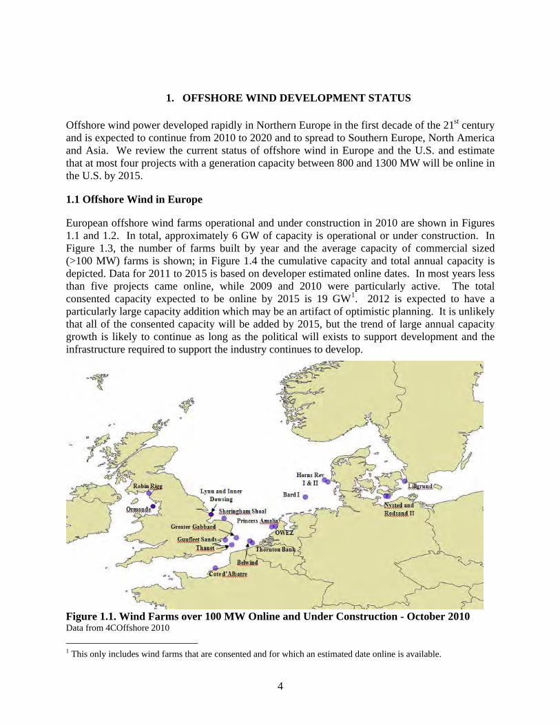
Offshore wind power developed rapidly in Northern Europe in the first decade of the 21st century and is expected to continue from 2010 to 2020 and to spread to Southern Europe, North America and Asia. We review the current status of offshore wind in Europe and the U.S. and estimate that at most four projects with a generation capacity between 800 and 1300 MW will be online in the U.S. by 2015.

1.1 Offshore Wind in Europe

European offshore wind farms operational and under construction in 2010 are shown in Figures 1.1 and 1.2. In total, approximately 6 GW of capacity is operational or under construction. In Figure 1.3, the number of farms built by year and the average capacity of commercial sized (>100 MW) farms is shown; in Figure 1.4 the cumulative capacity and total annual capacity is depicted. Data for 2011 to 2015 is based on developer estimated online dates. In most years less than five projects came online, while 2009 and 2010 were particularly active. The total consented capacity expected to be online by 2015 is 19 GW1. 2012 is expected to have a particularly large capacity addition which may be an artifact of optimistic planning. It is unlikely that all of the consented capacity will be added by 2015, but the trend of large annual capacity growth is likely to continue as long as the political will exists to support development and the infrastructure required to support the industry continues to develop.

Figure 1.1. Wind Farms over 100 MW Online and Under Construction - October 2010 Data from 4COffshore 2010

1 This only includes wind farms that are consented and for which an estimated date online is available.

5

Figure 1.2. Capacity of European Offshore Wind Farms, Online and Under Construction as of October 2010 Data from 4COffshore 2010

Figure 1.3. Number of Offshore Wind Farms Built per Year and Average Capacity of New Farms Greater than 100 MW Data from 4COffshore 2010; industry press

6

Figure 1.4. Offshore Wind Capacity Additions and Cumulative Capacity Data from 4COffshore 2010; industry press Table 1.1 shows offshore wind capacity by nation and total consented, generating, and under construction capacity. The total capacity is 24.5 GW. Total capacity is greater than capacity online by 2015 (19 GW) due to several large consented farms which are not planned to be online before 2015. As of October 2010, the UK had the largest wind generation capacity in Europe with 1,341 MW of nameplate capacity and 971 MW under construction. This represents 44% of European offshore wind capacity and 41% of capacity under construction. In 2011, offshore wind is expected to account for 1 to 2% of UK electricity generation2. Including consented projects, Germany has 9 GW of offshore wind capacity which, if built, would account for 4 to 5% of national generation. Thus, in the near to mid-term offshore wind in Europe will be a small but not insignificant contributor to total electrical generation. Planned offshore wind farms in Europe are geographically concentrated. Figure 1.5 shows the planned offshore wind farms in the German sector of the North Sea; Figure 1.6 shows development for Round 1 and 2 in the UK’s Thames estuary. Similar patterns hold for parts of Denmark, the Netherlands and Belgium. The density of offshore wind concessions illustrates the enthusiasm for offshore wind development among European policy makers and the relative lack of conflict with other users of the North Sea. Growth in the European offshore market will depend principally on the ability of developers to manage cost and the supply chain to meet demand. Growth across the entire supply chain is required if European nations are to meet national targets. Specifically, newbuilt installation 2 Assuming a capacity factor of 0.35 and national production similar to 2005-2010 average.

7

vessels, additional foundation manufacturing capacity, and the development of specialized offshore wind turbines with their own manufacturing supply chain independent of the onshore wind industry are required (EWEA 2009).

Table 1.1. Offshore Wind Capacity by Nation – October 2010 Nation Consented

(MW) Under Construction

(MW) Operational

(MW) Total (MW)

United Kingdom 2,596 971 1,341 4,908 Denmark 418 7 855 1,280 Belgium 864 330 300 1,494 Netherlands 3,250 0 247 3,497 Sweden 1,266 0 164 1,430 Germany 8,657 448 73 9,178 Finland 400 0 30 430 Ireland 0 0 25 25 Norway 365 0 2 367 Romania 500 0 0 500 Estonia 1,000 0 0 1,000 Italy 162 92 0 254 France 0 105 0 105 Total 19,078 2,353 3,037 24,468 Data from 4COffshore 2010; Industry press

Figure 1.5. Offshore Wind Farms Planned for the German Sector of the North Sea Source: BSH 2010

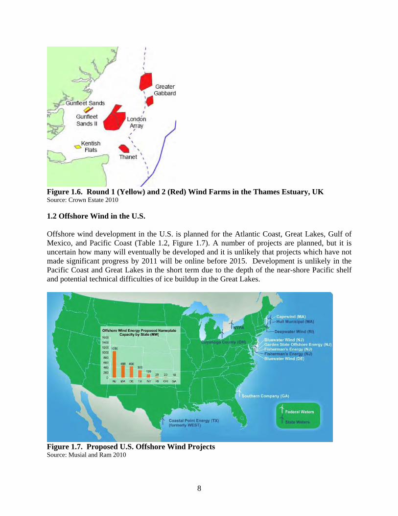
8

Figure 1.6. Round 1 (Yellow) and 2 (Red) Wind Farms in the Thames Estuary, UK Source: Crown Estate 2010

1.2 Offshore Wind in the U.S. Offshore wind development in the U.S. is planned for the Atlantic Coast, Great Lakes, Gulf of Mexico, and Pacific Coast (Table 1.2, Figure 1.7). A number of projects are planned, but it is uncertain how many will eventually be developed and it is unlikely that projects which have not made significant progress by 2011 will be online before 2015. Development is unlikely in the Pacific Coast and Great Lakes in the short term due to the depth of the near-shore Pacific shelf and potential technical difficulties of ice buildup in the Great Lakes.

Figure 1.7. Proposed U.S. Offshore Wind Projects Source: Musial and Ram 2010

Table 1.2. Proposed U.S. Offshore Wind Farms and Development Status – October 2010 Developer Wind Park Location Jurisdiction Capacity

(MW)Online by

2015* Status

EMI Cape Wind Cape Cod Federal 468 L Commercial lease executed; PPA signed; awaiting financing

Coastal Point Galveston Offshore Wind Galveston State 150 L Lease issued; waiting on Corps of Engineers approval

Coastal Point Jefferson, Brazoria, Corpus Christi, & Brownsville

Texas State 1800 U Lease issued.

NYPA Long Island Offshore Wind Park

Long Island Federal 350-700 U On-hold for several years; recently applied for BOEMRE limited lease

Bluewater Wind Delaware Federal 200-600 L PPA signed; BOEMRE limited lease issued

Southern Company Georgia Federal U Offered BOEMRE lease; not executed

Hull Municipal Hull Offshore Wind Massachusetts State 12-20 U Estimated development costs prohibitive; unlikely to move forward

Deepwater Wind Block Island Rhode Island State 29 L PPA signed Deepwater Wind Garden State Offshore Energy New Jersey Federal 350 P BOEMRE limited lease issued Fisherman’s Energy New Jersey Federal 330 P BOEMRE limited lease issued Fisherman’s Energy Atlantic City New Jersey State 20 L Applied for state permits;

launched wind monitoring buoyBluewater Wind New Jersey Federal 350 P BOEMRE limited lease issued Baryonyx Rio Grande Texas State 1000-1200 U State lease issued Baryonyx Mustang Island Texas State 1000-1200 U State lease issued GLOW/LEEDCo Cuyahoga Lake Erie State 20 L Agreed to supply contract with

GE NYPA Great Lakes State 120-500 U Issued RFP Total 6199-7737

Note: * L denotes likely; P denotes possible; U denotes unlikely

10

11

Demonstration and commercial projects are planned in both state and federal waters. Large scale developments in state waters are most advanced in Texas, but development could also occur offshore Maine, New York and Massachusetts, and possibly in the Great Lakes. One of the main obstacles for state water development is the aesthetic buffer that coastal residents may demand. Most development is expected to occur in federal waters, particularly the Northern and Mid-Atlantic regions (Figure 1.8) where wind speeds are highest, state renewable portfolio standards exist, high population densities are found, and capacity limitations and transmission bottlenecks occur. The South Atlantic region has a geographic advantage since the continental shelf is particularly shallow, but wind speeds are lower and onshore generation capacity is not as constrained.

Figure 1.8. BOEMRE Planning Areas Source: BOEMRE 2010 The Bureau of Ocean Energy Management, Regulation, and Enforcement (BOEMRE) have issued three limited leases offshore New Jersey and one lease off of Delaware for resource evaluation. Limited leases allow for the construction of met towers and other monitoring activities, but do not allow for commercial development. The New Jersey leases were awarded to Fisherman’s Energy, Bluewater Wind and Deepwater Wind. The Delaware lease was issued to Bluewater Wind. Southern Company was offered a limited lease offshore Georgia but it has not been executed (Musial and Ram 2010). Table 1.2 summarizes the most advanced projects in federal and state waters which we classify as likely, possible, and unlikely to be online by 2015 corresponding to our subjective assessment of a 90%, 50%, and 10% chance of installation. The judgments are speculative but are based on the status and size of the project, the financial capacity of the developer, regulatory evolution, local political enthusiasm, and expected economic conditions. We also assume that an adequate supply chain develops in the region. Negative movement in any of these factors will impair

12

progress in development. We estimate that nameplate online capacity in 2015 will be on the order of 887 to 1,287 GW. A description of projects most likely to begin construction follows. 1.2.1 Cape Wind Cape Wind is planned in Nantucket Sound on the south side of Cape Cod (Figure 1.9). It is approximately 6 miles from land and in a relatively shallow (3 to 15 m) area called Horseshoe Shoals. The Cape Wind project is to be composed of 130, 3.6 MW turbines placed on monopile foundations. Total nameplate capacity is 468 MW and it will be one of the largest offshore wind developments in the world. The staging area is to be Quonset, Rhode Island, approximately 100 km from the offshore site. The development plan is very similar to those undertaken in existing commercial offshore wind farms in Europe.

Figure 1.9. Proposed Cape Wind Turbine and Cable Array Source: MMS 2008 Cape Wind was originally proposed in 2001 and was under the jurisdiction of the Army Corps of Engineers; in 2005 jurisdiction was assigned to BOEMRE. Cape Wind was approved for

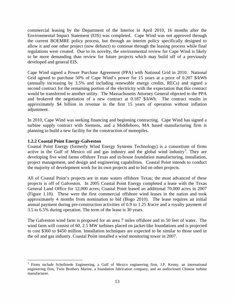
13

commercial leasing by the Department of the Interior in April 2010, 16 months after the Environmental Impact Statement (EIS) was completed. Cape Wind was not approved through the current BOEMRE policy process, but through an interim policy specifically designed to allow it and one other project (now defunct) to continue through the leasing process while final regulations were created. Due to its novelty, the environmental review for Cape Wind is likely to be more demanding than review for future projects which may build off of a previously developed and general EIS. Cape Wind signed a Power Purchase Agreement (PPA) with National Grid in 2010. National Grid agreed to purchase 50% of Cape Wind’s power for 15 years at a price of 0.207 $/kWh (annually increasing by 3.5% and including renewable energy credits, RECs) and signed a second contract for the remaining portion of the electricity with the expectation that this contract would be transferred to another utility. The Massachusetts Attorney General objected to the PPA and brokered the negotiation of a new contract at 0.187 $/kWh. The contract results in approximately $4 billion in revenue in the first 15 years of operation without inflation adjustment. In 2010, Cape Wind was seeking financing and beginning contracting. Cape Wind has signed a turbine supply contract with Siemens, and a Middleboro, MA based manufacturing firm is planning to build a new facility for the construction of monopiles. 1.2.2 Coastal Point Energy-Galveston Coastal Point Energy (formerly Wind Energy Systems Technology) is a consortium of firms active in the Gulf of Mexico oil and gas industry and the global wind industry3. They are developing five wind farms offshore Texas and in-house foundation manufacturing, installation, project management, and design and engineering capabilities. Coastal Point intends to conduct the majority of development work for its own projects and to bid on other projects. All of Coastal Point’s projects are in state waters offshore Texas; the most advanced of these projects is off of Galveston. In 2005 Coastal Point Energy completed a lease with the Texas General Land Office for 12,000 acres; Coastal Point leased an additional 70,000 acres in 2007 (Figure 1.10). These were the first commercial offshore wind leases in the nation and took approximately 4 months from nomination to bid (Bogo 2010). The lease requires an initial annual payment during pre-construction activities of 0.9 to 1.25 $/acre and a royalty payment of 3.5 to 6.5% during operation. The term of the lease is 30 years. The Galveston wind farm is proposed for an area 7 miles offshore and in 50 feet of water. The wind farm will consist of 60, 2.5 MW turbines placed on jacket-like foundations and is projected to cost $360 to $450 million. Installation techniques are expected to be similar to those used in the oil and gas industry. Coastal Point installed a wind monitoring tower in 2007.

3 Firms include Schellstede Engineering, a Gulf of Mexico engineering firm, J.P. Kenny, an international engineering firm, Twin Brothers Marine, a foundation fabrication company, and an undisclosed Chinese turbine manufacturer.

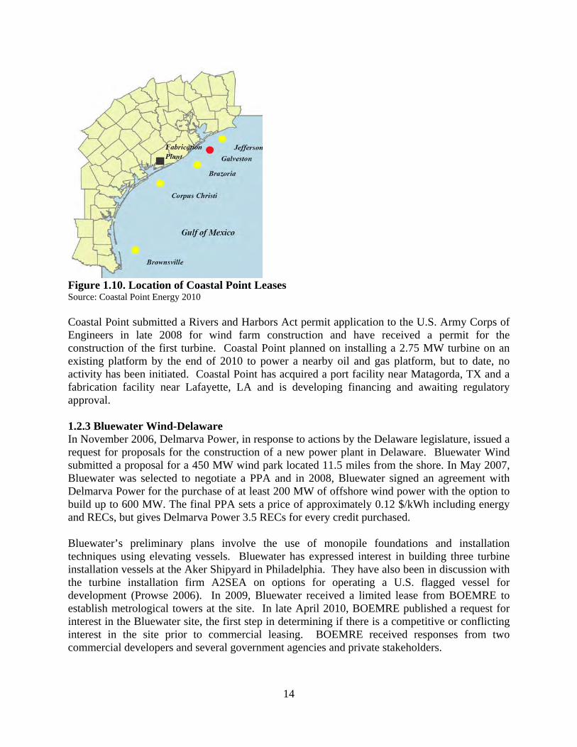
14

Figure 1.10. Location of Coastal Point Leases Source: Coastal Point Energy 2010 Coastal Point submitted a Rivers and Harbors Act permit application to the U.S. Army Corps of Engineers in late 2008 for wind farm construction and have received a permit for the construction of the first turbine. Coastal Point planned on installing a 2.75 MW turbine on an existing platform by the end of 2010 to power a nearby oil and gas platform, but to date, no activity has been initiated. Coastal Point has acquired a port facility near Matagorda, TX and a fabrication facility near Lafayette, LA and is developing financing and awaiting regulatory approval. 1.2.3 Bluewater Wind-Delaware In November 2006, Delmarva Power, in response to actions by the Delaware legislature, issued a request for proposals for the construction of a new power plant in Delaware. Bluewater Wind submitted a proposal for a 450 MW wind park located 11.5 miles from the shore. In May 2007, Bluewater was selected to negotiate a PPA and in 2008, Bluewater signed an agreement with Delmarva Power for the purchase of at least 200 MW of offshore wind power with the option to build up to 600 MW. The final PPA sets a price of approximately 0.12 $/kWh including energy and RECs, but gives Delmarva Power 3.5 RECs for every credit purchased. Bluewater’s preliminary plans involve the use of monopile foundations and installation techniques using elevating vessels. Bluewater has expressed interest in building three turbine installation vessels at the Aker Shipyard in Philadelphia. They have also been in discussion with the turbine installation firm A2SEA on options for operating a U.S. flagged vessel for development (Prowse 2006). In 2009, Bluewater received a limited lease from BOEMRE to establish metrological towers at the site. In late April 2010, BOEMRE published a request for interest in the Bluewater site, the first step in determining if there is a competitive or conflicting interest in the site prior to commercial leasing. BOEMRE received responses from two commercial developers and several government agencies and private stakeholders.

15

1.2.4 Deepwater-Rhode Island In 2008, Rhode Island solicited bids for the development of a commercial scale offshore wind farm. Deepwater Wind (formerly Winergy) was selected in early 2009. Two projects are planned; a small, 8 turbine, 29 MW wind farm off of Block Island in state waters, and a farm composed of 107, 3.6 MW turbines (385 MW) approximately 20 miles offshore in 40 to 45 m water depths. Deepwater Wind has developed a novel4 plan for installing turbines, but thus far, has not secured a limited lease from BOEMRE. Deepwater negotiated a 20 year PPA with National Grid for the purchase of electricity from the Block Island wind farm. The contract price was 0.244 $/kWh, but the contract was rejected by the Rhode Island Public Utility Commission for being too costly. After it was rejected, the Rhode Island legislature passed a law requiring the Public Utility Commission to re-evaluate the project against more lenient standards, but the law requires Deepwater to disclose its development costs and the PPA contains provisions for price reductions if costs are lower than anticipated. The Public Utility Commission approved the PPA, but the constitutionality of the law is being challenged in court. 1.2.5 Garden State Offshore Energy-New Jersey Deepwater Wind and PSEG Global, a sister company of New Jersey’s major regulated gas and electricity provider, plan to develop the Garden State Offshore Energy (GSOE) project, a 350 MW facility 17 miles off of New Jersey (Figure 1.11). GSOE began in response to a solicitation from the New Jersey Board of Public Utilities. The proposed technology is similar to that used in the Deepwater Rhode Island project. Deepwater received a limited lease from BOEMRE and plans to install a mobile wind monitoring buoy on the site in the near future.

1.3 Factors Impacting U.S. Development

Offshore wind development in the U.S. is expected to be constrained in the near term by three main factors: financing and PPAs, regulation, and the supply chain. A number of companies are interested in offshore wind development, however, their high costs and uncertain risks make financing difficult. Financing will rely on the ability of developers to negotiate favorable PPAs. Recently negotiated PPAs have provided developers with high expected returns, but have been challenged by regulators and politicians due to cost pass-through to ratepayers. The success of PPA’s will depend on local electricity markets, federal and state greenhouse gas policies and grid operators’ expectations of future hydrocarbon costs. One of the major impediments to the development of offshore wind may be the evolution of shale gas because plentiful natural gas supplies will translate to cheaper electric utility rates and large reserves will change utilities expectations of future electricity costs. The rate of leasing by BOEMRE in federal waters and regulatory approval by the Army Corps of Engineers in state waters is uncertain. Cape Wind has now been approved, but its lease was not processed through the new BOEMRE regulations. No federal commercial lease has been 4 Deepwater Wind plans on using 4-pile jacket foundations transported to site by barge. The complete turbine is expected to be assembled onshore (although one blade may be installed after clearing bridges) and skidded onto a specially constructed, H-shaped jackup barge. The barge will transport the turbine and jackup next to each foundation. The height of the barge’s deck will be elevated so that it is level with the top of the foundation and the turbine will be skidded over the foundation and secured.

16

awarded via the current BOEMRE regulations and the time between the Notice of Interest and the offer of a commercial lease and the time between submission and approval of a development plan are unknown.

Figure 1.11. Proposed Garden State Offshore Energy Project Source: Garden State Offshore Energy 2010 Offshore wind development cannot occur without a reliable and efficient supply chain. Turbine installation vessels may be particularly hard to procure. Assuming that the average time to install a 3.6 MW turbine is one week, approximately 2,000 boat days are required to install 1 GW of capacity. To install this capacity in four years, an average of at least two, and likely three vessels, would be required. This is a significant but manageable hurdle.

1.4 Atlantic Wind Connection

In October 2010, Google and Good Energies, an energy investment firm, announced plans to build a 6 GW HVDC transmission line in the federal waters of the Atlantic Ocean called the Atlantic Wind Connection. Initially, the plans call for a 150 mile cable connecting northern New Jersey to Delaware at a cost of $1.8 billion. The total project would run 350 miles from New Jersey to Norfolk, VA and cost $5 billion (Figure 1.12). The stated purpose of the cable is two-fold: to transport electricity from inexpensive markets in Virginia to more expensive markets in

17

New York and New Jersey and to bring offshore wind power to shore. If built, both the power capacity and the length would make it among the largest submarine cables in the world.

Figure 1.12. Proposed Atlantic Wind Connection and Hypothetical Wind Farms Source: Atlantic Wind Connection 2010 The transmission line may have positive effects on the offshore wind market, but may also create additional issues. The cable would likely smooth out fluctuations in power output from wind farms built along the route, making offshore wind more reliable and valuable (Kempton et al. 2010). Additionally, the cable could transmit power from areas where electricity prices are low, to higher price areas, potentially making the economics of development more favorable. However, the movement of offshore wind power from the area in which it is produced to another region may prove problematic for local stakeholders. The governors of several states (Delaware, Maryland, Rhode Island, New Jersey) have supported offshore wind power as a means of meeting state Renewable Portfolio Standards (RPS). However, if power generated off the coast of one state was sold to the grid operator in another state, the power would not count towards RPS goals and the public may be less likely to support offshore wind if the resultant electricity is exported to another state. Additionally, it is possible that the cable would not be economic for every wind farm. The decision to link into the Atlantic Wind Connection would be complex and based on the price structure of the local and terminal markets, transmission costs, the distance to shore, the capacity of the wind farm, expected capacity factor, and the costs of HVAC and HVDC substations. It is also not clear how much of the cable capacity would be dedicated to wind production. The AWC would likely be a merchant transmission line and may be allowed by the Federal Energy Regulatory Commission (FERC) to sell capacity based on negotiated rate-based contracts (rather than cost based contracts used for most generation). At least 50% of the capacity would be

18

allocated through a non-discriminatory, open-access auction, with the remaining 50% potentially sold to “anchor” customers. Thus, transmission rights would be allocated to the customers who are most capable and willing to pay for access and this may or may-not be offshore wind generators. There are a number of outstanding issues associated with the Atlantic Wind Connection that at present remain speculative.

2. OFFSHORE WIND ENERGY SYSTEM COMPONENTS

An offshore wind farm is a power plant that consists of a number of turbines connected with an internal grid for power transfer, one or more substations – located on or offshore – and an export cable to transmit the power to the local grid. Offshore wind farms are complex, capital intensive engineering projects in the early stages of technical development. The principal components include turbines, towers, foundations, electric collection and transmission systems, and other balance of plant items. The purpose of this chapter is to define the components of offshore wind systems.

2.1 Meteorological Systems

A meteorological mast (or met tower) is the first structure installed during the planning stages. The purpose of a met tower is to evaluate the meteorological environment and living resource data within the project area. Examples of the Cape Wind, Massachusetts, and Coastal Point Energy (formerly West), Texas, met towers are shown in Figure 2.1. A mast consists of a foundation, platform with boat loading, meteorological and other instrumentation, navigational lights and marking, and related equipment. A met tower is installed in a manner similar to a monopole foundation or jacket structure, but the diameter and weight is considerable smaller.

Figure 2.1. Cape Wind (Left) and Coastal Point Energy Meteorological Towers Source: Cape Wind 2010; Coastal Point Energy 2010

19

A mast collects wind data at multiple heights by intersecting the wind with an anemometer to verify the project area’s meteorology. Sensors also collect data on: vertical profiles of wind speed and direction; air temperature and barometric pressure; ocean current velocity and direction profiles; sea water temperature; marine mammal presence; avian presence; bat presence. Permit authorizations for the installation of monitoring systems are obtained through the U.S. Army Corps of Engineers (Nationwide permits 5&6), the U.S. Coast Guard (Private Aids to Navigation) and the BOEMRE (Limited lease). The data from the meteorological mast serves to test power performance, perform due diligence evaluation, and facilitate estimates of operation maintenance management. Ideally, a met-tower should be located upwind of the project area in the prevailing wind direction.

2.2 Support System

The support system refers to the foundation, transition piece, and scour protection. The primary purpose of the foundation is to support the turbine. A transition piece is attached to the foundation to absorb tolerances on inclination and simplify tower attachment. Scour protection helps to ensure that environmental conditions do not degrade the mechanical integrity of the support system. 2.2.1 Foundation Foundation technology is designed according to site conditions. Maximum wind speed, water depth, wave heights currents, and surf properties affect the foundation type and design. The size and weight of the turbine and tower are also key components. Within a wind farm, each foundation is customized to the water depth and soil type at its particular location. Extreme loading conditions and frequency are important design parameters. Four basic types of foundations have been used in offshore wind farms: monopiles, jackets, tripods and gravity foundation. Additionally, a single 2.3 MW demonstration turbine has been installed on a floating foundation. Foundations are prefabricated onshore in one piece, carried offshore by barge or towed, launched at sea, and set on bottom by a crane or derrick barge. Monopiles Monopiles are large diameter, thick walled, steel tubulars that are driven (hammered) or drilled (or both) into the seabed (Figure 2.2). Outer diameters usually range from 4 to 6 m and 40 to 50% of the length is inserted into the seabed. Design codes and standards specify the thickness and the depth the piling is driven depends on the design load, soil conditions5, water depth, and environmental conditions. Pile driving is more efficient and less expensive than drilling. Monopiles are currently the most common foundation in shallow water (less than 20 m) development (Table 2.1) due to its lower cost and simplicity, but because they are limited by depth and subsurface conditions, they will decline as wind development moves to deeper water. However, in nascent markets such as the U.S., and for the near term future, monopiles are expected to be heavily employed.

5 In soft soil regions, deeper piles and thicker steel are required.

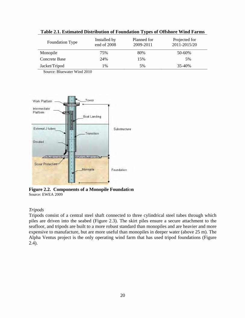
20

Table 2.1. Estimated Distribution of Foundation Types of Offshore Wind Farms

Foundation Type Installed by end of 2008

Planned for 2009-2011

Projected for 2011-2015/20

Monopile 75% 80% 50-60% Concrete Base 24% 15% 5%

Jacket/Tripod 1% 5% 35-40% Source: Bluewater Wind 2010

Figure 2.2. Components of a Monopile Foundation Source: EWEA 2009 Tripods Tripods consist of a central steel shaft connected to three cylindrical steel tubes through which piles are driven into the seabed (Figure 2.3). The skirt piles ensure a secure attachment to the seafloor, and tripods are built to a more robust standard than monopiles and are heavier and more expensive to manufacture, but are more useful than monopiles in deeper water (above 25 m). The Alpha Ventus project is the only operating wind farm that has used tripod foundations (Figure 2.4).

21

Figure 2.3. Components of a Tripod Foundation Source: EWEA 2009

Figure 2.4. The Taklift 4 Placing a Tripod Foundation at Alpha Ventus Source: Alpha Ventus 2010

22

Jackets Jacket foundations are an open lattice steel truss template consisting of a welded frame of tubular members extending from the mudline to above the water surface (Figure 2.5). Piling6 is driven through each leg of the jacket and into the seabed to secure the structure against lateral forces. Jackets are robust and heavy structures and require expensive equipment to transport and lift. To date, jacket foundations have not been used extensively due to the preference for shallow, near shore environments. At around 50 m, jacket structures are required. Jackets have been used for two of the deepest developments, Beatrice (45 m) and Alpha Ventus (30 m), supporting large 5 MW turbines. Jackets are also commonly used to support offshore substations (Figure 2.6). Theoretically, jackets can be used in deep water (100s of meters), although economic considerations may limit their deployment to water under 100 m.

Figure 2.5. Components of a Jacket Foundation Source: EWEA 2009

6 Jackets and tripods are attached to the subsurface using piles. However, designs could be modified to use suction caissons. In this case, a cylindrical steel caisson (resembling an overturned bucket) is allowed to sink to the seabed under its own weight (Byrne et al., 2002). Suction is then applied to the inside of the caisson and water is pumped out. The resulting pressure differential causes the caisson to be driven into the seabed.

23

Figure 2.6. A Jacket Structure Supports the Substation at Alpha Ventus Source: Alpha Ventus 2010 Gravity Foundations Gravity foundations are concrete structures that use their weight to resist wind and wave loading (Figure 2.7). Gravity foundations require unique fabrication facilities capable of accommodating their weight (either drydocks, reinforced quays or dedicated barges). Gravity foundations have been used at several offshore wind farms, including Middelgrunden, Nysted, Thornton Bank and Lillgrund. Gravity foundations are less expensive to build than monopiles, but the installation costs are higher, due largely to the need for dredging and subsurface preparation and the use of specialized heavy-lift vessels (Figure 2.8). The deepest gravity foundations in operation are in Thornton Bank (27 m). Gravity foundations are most likely to be used where piles cannot be driven and the region has dry-dock facilities for concrete construction (Volund 2005). In the North Sea, gravity foundations have also been used in the offshore oil and gas industry, but in the U.S. there has been no use of concrete structures for offshore oil and gas operations and no plan to use them in offshore wind development. In Europe, gravity foundations will likely continue to fill an important niche for shallow to moderate water depth wind farms where drivability is a concern. However, they are unlikely to be widely used (if at all) in the U.S. waters.

24

Figure 2.7. Components of a Gravity Foundation Source: EWEA 2009 Floating Structures As water depth increases, the use of a steel platform will be limited by economic considerations. In the offshore oil and gas industry, the water depth limit for fixed platforms is about 450 m (1,500 ft), but in the offshore wind industry, the limit is likely to be less than 100 m. Floating structures consist of a floating platform and an anchoring system. There are several alternative designs for floating turbine foundations all of which are variations on the spar and tension-leg concepts in the oil and gas industry (Figure 2.9). The Hywind concept is being developed by Statoil Hydro. A pilot turbine was placed in waters off Norway in summer 2009 (Figure 2.10). The foundation consists of an 8.3 m diameter, 100 m long submerged cylinder secured to the seabed by three mooring cables. Hywind was towed horizontally to a fjord and partially flooded and righted. Additional ballast was then added and the turbine was installed on top. The assembled turbine was towed out to sea and the anchors placed. Blue H has developed a deepwater concept based on the tension leg platform. A prototype has been deployed off the coast of Italy and another is planned off the southern coast of Massachusetts. The Blue H concept consists of a two blade turbine placed on top of a buoyant, semi-submerged steel structure attached to a counterweight on the seabed. Plans are to assemble the turbine and foundation onshore and tow it to the offshore site.

25

Figure 2.8. The Eide Barge 5 Lifting a Gravity Foundation at Nysted Source: DONG Energy 2010a.

Figure 2.9. The Hywind Turbine and Support Structure Source: StatoilHydro 2009

Figure 2.10. The Hywind Turbine being Towed Offshore Source: StatoilHydro 2010 2.2.2 Transition Piece After the foundation is installed, a transition piece is placed on top of the foundation to levelize horizontal inaccuracies (Figure 2.11). Transition pieces pass through the majority of the water column but do not rest on the seabed; boat fenders, access ladders, access deck, handrails are

26

attached on the outside, and electrical components such as a transformer, switchgear, control equipment, and cables may be included. For monopole foundations, the gap between the pile and transition piece is normally filled with cement grout. For jackets and gravity foundations, transition pieces are installed in port and would not require a separate offshore lift, and do not contain boat landings, electrical conduits or other accessory components as these are installed elsewhere on the foundation.

Figure 2.11. Transition Piece at Horns Rev II Source: DONG Energy 2010b 2.2.3 Scour Protection When a structure is placed in a current and the seabed is erodible, scour may lead to structural instability. Scour refers to the removal of sediment from the area around the base of a support structure. Scour protection requirements depends on the current and wave regime at the site, the substrate and foundation type. Low tech and relatively inexpensive methods are usually adequate to address the problem. Commonly employed measures of scour protection include dumping rock of different grade and placing concrete mattresses around the foundation. For monopole foundations, a layer of small rocks may be installed prior to or following pile driving; later, after cabling is installed, large cover stones may be placed around the foundation (Gerwick 2007). Monopiles, gravity foundations, and tripods require significant scour protection, while piled jackets require little or no scour protection (den Boon et al., 2004; Seidel 2007; Larsen et al., 2005). In some cases, the entire wind farm may be enclosed by a rock wall to minimize currents and scour.

27

2.3 Wind Turbine

The wind turbine refers to a collection of components: Tower Nacelle Hub Blades

The tower is attached to the transition piece, and the nacelle is attached to the tower, followed by the hub and one or more blades (Figure 2.12). There are several different options for installation which will be discussed in the next chapter. The blades and hub are also called the rotor.

Figure 2.12. An Assembled Rotor Being Lifted onto a Nacelle at Nysted Source: DONG Energy 2010a Offshore turbines range from 2 to 5 MW and typical weights of the components are shown in Table 2.2. Component size and weight varies with the electrical capacity of the turbine, the rotor dimensions, and the selection of blade, hub, and nacelle material and equipment. Turbines are an established commodity but offshore technology is still in the early stages of evolution and will continue to develop in the future. Clipper, AMSC and Dongfang are all reported to be developing 10 MW offshore turbines.

Table 2.2. Weights of Commonly Used Offshore Turbines Turbine Capacity (MW) Blade length (m) Tower (t) Rotor (t) Nacelle (t) Siemens 3.6-107 3.6 52 180-200 95 125 Vestas V90-3 MW 3 44 100-150 42 70 Repower 5 M 5 61.5 210-225 120 300

Source: Company data

28

Tower The tower provides support to the turbine assembly and the balance of plant components, including a transformer located in the base7, a yaw motor located at the top, communication and power cables. The tower also provides a ladder and/or an elevating mechanism to provide access to the nacelle. Towers are tubular structures consisting of steel plate cut, rolled, and welded8 together into large sections. In installation, tower sections are bolted to each other during assembly, or are pre-assembled at port. Tower height is determined by the diameter of the rotor and the clearance above the water level. Typical tower heights are 60 to 80 m giving a total hub height of 70 to 90 m when added to the foundation height above the water line. Tower diameter and strength depend on the weight of the nacelle and expected wind loads. Nacelle The nacelle houses the generator, gearbox, and monitoring, communications, control and environmental maintenance equipment (Figure 2.13). The nacelle is principally composed of a main frame and cover. The main frame is the element to which the gearbox, generator and brake are attached, and must transmit all the loads from the rotor and reaction loads from the generator and break to the tower (Manwell et al. 2002). Nacelles are large units and typically the heaviest and highest lift. The relative size of a nacelle is depicted in Figure 2.14. Hub The hub is a cast steel structure. The hub transmits horizontal wind loads from the blades to the nacelle, transmits rotational energy to the gearbox via a low speed shaft, and is one of the most highly stressed components of the turbine (Hau 2006). The hub also contains motors for controlling blade pitch. Blades Blades are airfoils made of composite or reinforced plastics. The blades are bolted to the hub either onshore or offshore. Due to their construction materials, low weight, and long length (50 to 60 m), blades are sensitive to high winds during lifting operations. The size and shape of assembled configurations complicates onshore and offshore transport.

2.4 Electricity Collection and Transmission

Cables connect the turbines and the wind farm to the electrical grid. Collection cables connect the output of strings (rows) of turbines depending on the configuration and layout of the wind farm. The output of multiple collection cables are then combined at a common collection point or substation for transmission to shore.

7 The turbine transformer is either located up tower in the nacelle or at the base of the turbine (down tower). Turbine transformers take the energy generated by the turbine and convert it to approximately 34.5 kV for connection with the collection system. 8 Manufacturers purchase steel as hot-rolled plates which are cold rolled and welded using standard machinery.

29

Figure 2.13. Diagram of a Nacelle Source: DOE 2010

Figure 2.14. Inside of a Nacelle and Relative Size Source: Vattenfall 2010 Inner–Array Cable The inner-array cables connect the wind turbines within the array to each other and to an offshore substation if present. The turbine generator is low voltage (usually, less than 1 kV, often 500 to 600 V) which is not high enough for direct interconnection to other turbines. A turbine transformer steps up the voltage to 10 to 36 kV for cable connection. Inner-array cables are connected to the turbine transformer and exit the foundation near the mudline. The cables are buried 1 to 2 m below the mudline and connect to the transformer of the next turbine in the string. The power carried by cables increases as more turbines are connected and the cable voltage may increase to handle the increased load. The amount of cabling required depends on

30

the layout of the farm, the distance between turbines, and the number of turbines. Cable layouts for Lillgrund and Middelgrunden are depicted in Figures 2.15 and 2.16. The hole in the center of Lillgrund is due to shallow water.

Figure 2.15. Layout of Lillgrund Source: Jeppson et al., 2008 Export Cable Export cables connect the wind farm to the onshore transmission system. Export cables are buried to ensure that they do not become exposed, and in some places, export cables may require scour protection. At the beach, cables will come onshore and may be spliced to a similar cable and/or connected to an onshore substation. Water depths along the cable route, soil type, coastline types, and many other factors determine the cable route, time and cost. At the onshore substation or switchyard, energy from the offshore wind farm is delivered to the power grid. If the point of interconnection (POI) voltage is different from the submarine transmission, transformers are used to match the POI voltage; otherwise, a switchyard is used to directly interconnect the wind farm. At this point, power generated is metered and purchased via a Power Purchase Agreement with a local utility or by entering the Independent System Operator's merchant market.

31

Figure 2.16. Layout of Middelgrunden Source: Middelgrundens Vindmollelaug 2010 Export cables are composed of three insulated conductors protected by galvanized steel wire. Medium voltage cables are used when no offshore substation is installed and usually range between 24 to 36 kV. High voltage cables are typically 110 to 150 kV and are used with offshore substations. High voltage cables are able to carry more power than a medium voltage cable but are heavier and wider in diameter. High voltage cable may weigh 50 to 100 kg/m while medium voltage cable may weigh 20 to 40 kg/m.

2.5 Offshore Substation

The purpose of an offshore substation is to minimize transmission losses by transforming the voltage of the electricity generated at the wind turbine to a higher voltage suitable for transmission to shore. The substation is sized with the appropriate power rating (MVA) for the project capacity, and steps up the line voltage from the collection system voltage to a higher voltage level, usually that of the POI. Power that flows on higher voltage lines will minimize line loss and increase the overall efficiency of the system. All offshore wind farms require substations, but not all substations are located offshore. The need for offshore substations depends upon the power generated and the distance to shore which determines the tradeoffs between capital expenditures and transmission losses (Wright et al., 2002). The components of offshore substations include voltage transformers, switchgear, back up diesel generator and tank, accommodation facilities, j-tubes, and medium and high voltage cables

32

(Figure 2.17). Substations are positioned within the wind farm at a location that minimizes export and inner-array cable distance. Substations are typically 500 tons or more and are placed on foundations similar to those used for turbines. Onshore substations also include equipment to monitor power quality, such as voltage stability and harmonic disturbances, and SCADA systems allow the behavior of the entire system to be monitored and controlled.

Figure 2.17. Substation Being Lifted onto Monopile at Gunfleet Sands Source: Offshore Wind Power Marine Services 2010

2.6 Commissioning

Commissioning refers to the activities after all components are installed but before commercial operations begin. This includes electrical testing, turbine and cable inspection, and related quality control activities. The communication and control systems are tested to enable the turbine controllers to be accessed remotely from the control room.

33

3. STAGES OF OFFSHORE DEVELOPMENT

There are many steps involved in developing an offshore wind farm. The objective of the developer is to recover costs and maximize profits while the objective of the landowner varies with ownership. A private owner will typically want to maximize income while public ownership requires environmental stewardship, a fair return on use, development goals, and other objectives. The purpose of this chapter is to outline the stages of offshore wind development and review the structure of existing state and federal offshore wind leases. We begin by defining project location.

3.1 Project Location

Offshore areas are subject to various federal and state authorities. Which federal agency has lead responsibility for regulatory oversight depends on the location and type of project. Depending on the specific locale, more than one state or federal agency may exercise jurisdiction. All offshore jurisdictions are defined in reference to the following technical demarcations. 3.1.1 Baseline The baseline is the boundary line dividing the land from the ocean and is described in terms of nautical9 mile (nm). The baseline is defined as the mean low lower water level along the coast as shown on official U.S. nautical charts. It is drawn across the mouths of rivers and the entrances to bays, and along the outer points of complex coastlines. 3.1.2 State Waters Generally, offshore state waters cover the area from the baseline out 3 nm, although it is to 9 nm for the offshore Gulf coasts of Texas and Florida, as well as Puerto Rico. This area of state jurisdiction was granted by the Submerged Lands Act of 1953 (43 U.S.C. §1301 et seq.). The federal government may regulate commerce, navigation, power generation, national defense, and international affairs within this area, while states have the authority to manage, develop, and lease resources throughout the water column as well as on and under the associated sea bed. 3.1.3 Outer Continental Shelf The federal government administers the outer continental shelf (OCS), which comprises the submerged lands, subsoil, and sea bed lying between the seaward extent of the states’ jurisdiction and the seaward extent of federal jurisdiction. Typically, this is the area between three and 200 nm.

3.2 Development Process

3.2.1 Lease Acquisition The first step in developing an offshore wind farm is to acquire a wind lease from the landowner. For offshore wind, the landowner is either the state or federal government, depending on the location of the site. For public lands, the government is responsible to ensure environmentally

9 A nautical mile is 1.15 statute miles.

34

sound and safe development and a fair return to the public. All lease terms and provisions are negotiated in advance and are publicly disclosed. 3.2.2 Assessment After a company acquires a lease, the next step in development is to determine the wind potential and conduct preliminary environmental studies. During assessment, engineering studies are performed, and if the property is considered commercially viable, financing is arranged, power purchase agreements are negotiated, and the capacity and placement of turbines is determined. If the property is not suitable for development because of its wind resources or other impediments such as permitting problems, transmission interconnection issues, unfavorable power purchase price, or financing constraints, the wind lease terminates or the company does not exercise its option to develop. For commercially viable projects, the next stage is design and construction. 3.2.3 Design Offshore wind projects are designed for the location in which they operate. Because every location is unique in terms of geological factors (seabed depths and morphology, seafloor composition, geology, seabed stability), meteorology and oceanography (wind, waves, currents, tidal range, seasonality), man-made factors (port infrastructure, shipping density, restricted areas, commercial fishing activities, oil and gas development, pipelines, submarine cables, buoys, dredging activity, shipwrecks, coastal construction, security threats), environmental factors (benthic, fish and shellfish, birds, marine mammals), landing site (utilities, geology, beach and near shore stability, weather exposure, environmental factors), and permitting, every project is unique in its scope, development, and installation. 3.2.4 Construction Construction activities include the procurement of goods, fabrication, assembly, and installation processes. Fabrication, assembly and installation is the second largest cost category behind procurement. Construction normally includes the raw material cost (e.g., steel) and the cost to fabricate piling, transition pieces, and jacket structures, as well as the cost to assemble turbines. Fabrication may occur at the staging area or another location, and depending on the degree of integration and pre-assembly required, one or more staging areas may be employed. Procurement and Delivery Procurement and delivery involves acquiring equipment and delivering it to the staging area. Equipment includes meteorological instruments, turbines (towers, nacelles, hub, blades), cable, transformers, supervisory control and data acquisition (SCADA) systems, fiber optics, and other goods that do not require fabrication. Turbines are the primary capital expenditure and are purchased according to a fixed cost and schedule of delivery. Turbines are delivered to the staging area and assembled according to the installation strategy. Turbines with the same generating capacity can have different weights, costs, and reliabilities and developers will base selection on a combination of these factors. The capacity of the turbine will determine the number required and the model will set lift weights and vessel capabilities. Similarly, the decision to install high or medium voltage cable, and the voltage and weight of that cable will impact capital and installation costs. Fabrication and Assembly

35

Foundations and transition pieces will be constructed near or at the staging area from sheet steel, or may be delivered to site via road, rail or barge. Assembly activities may occur onshore or offshore and the degree of onshore assembly will impact installation costs. By reducing the number of offshore lifts, the time required by the installation vessel will decline but the lifting capacity requirements will increase. At the extreme, a complete turbine assembly will require one lift using a heavy-lift vessel. Installation After a suitable number of turbines and/or foundations are available at the staging area, offshore installation may begin; however, if supply disruptions and delays occur, this will have significant negative consequences on installation expenditures. Installation occurs over three primary stages according to the unit being installed:

Foundation Turbines Cable

One or more marine vessels is required and the installation activities may be performed together or independent of one another. The basic process flow is as follows:

(1) Installation of the foundation, transition piece and scour protection; (2) Erection of the tower and turbine; (3) Installation of the electric service platform (if applicable); (4) Installation of the inner-array cables and scour protection; (5) Installation of the export cables and onshore transition.

Installation is defined as all activities to transport and install wind farm components from the onshore staging base to the onshore transition of the export cable. These activities include the cost to load the foundations, transition pieces, tower, turbines, substation, and cables from port; the cost to transport and install/erect individual elements; and all the support vessels directly associated with the operation (e.g., crew boats, tugs, and supply vessels) and may not be distinguished. Offshore substation installation costs are included, but after cables reach shore, the costs to build (or upgrade) an onshore substation and onshore grid connection may or may not be included depending on the system boundary. 3.2.5 Commissioning After a wind farm is tested and commissioned, it is ready for commercial production and power injection into the grid.

3.3 Texas Offshore Wind Lease Terms and Conditions

3.3.1 General Conditions Authority The Commissioner of the Texas General Land Office (GLO) acts for and on behalf of the Permanent School Fund, and grant leases of state-owned lands to pursue wind development. Money earned by the Land Office is constitutionally dedicated to the Texas Permanent School Fund. Granting Clause

36

The granting clause provides the lessee the exclusive right to research and develop wind resources, to convert wind resources on the leased premises to electricity, and to collect and transmit that electricity to market. Phases of the Lease The terms and conditions of offshore leases are defined in terms of two phases:

Phase I: Research and Analysis Phase II: Development and Production

Phase I is the research and analysis phase of the lease, where under an approved research plan, the lessee studies the wind resources at the site through meteorological towers, and performs other tests, such as soil and water samples, to determine the feasibility of commercial wind development. Phase I is of fixed duration and may be extended at the discretion of the GLO. Environmental studies on avian and bat interaction and migration patterns are required to be performed during this time, and the lessee is required to submit progress reports on a quarterly basis and a final report. At the end of Phase I, the lessee has an option to submit a production plan or to terminate the lease. In the case of termination, the lessee will need to remove all meteorological towers and instrumentation facilities, and any other improvements. Phase II of the lease is the construction and production phase, in which an approved production plan is constructed and wind electricity is generated. The duration of the construction period and option to extend depends on the size of the proposed facility and other factors specific to the lease. The construction period is typically for 30 years as long as there is commercial production of wind generated electricity. At the end of the production period, the lessee may enter into negotiations for a lease extension. At the end of Phase II, or in the case of default or termination, the lessee is required to return the greenfield status of the area. Reservations The full use of the leased premises, except for those granted to the lessee and to the extent that the use and/or rights do not materially interfere with the lessee’s operations, are reserved to the State of Texas. Additional use of the lease may include recreational activities or exploring for and producing the minerals that may be located within the surface boundaries of the premises. The lessee’s approved production plan contains the amount of acreage the lessee will retain for the project. The lessee also agrees to coordinate plans and cooperate on activities to minimize interference with other operations. Retained Acreage After production, the lessee will retain only that acreage that has been developed for production of wind electricity. Each wind turbine will retain an agreed amount of acreage, along with the wind easement, but all acreage outside the retained boundaries shall be released. Removal Deposits The lessee is required to deposit a bond, an irrevocable letter of credit, or a cash deposit in an amount sufficient to cover the surface and subsurface restoration costs and the estimated removal of the meteorological towers, wind turbines, and other related improvements prior to initiating

37

construction. In Phase I, the removal deposit is to be based on the estimated quantity or type of research equipment the lessee intends to install. In Phase II, the removal deposit is based on the estimated project capacity. In both cases, if the amount of research equipment or generation capacity exceeds the estimated quantities at the time the bond is invoked, an increase in the removal deposit may be required. Reporting Requirements Reporting requirements are made at every major milestone during each period. In Phase I, a research plan is submitted for review and approval before initiating any physical activities on the lease, consisting of: administrative information, projected schedule and discussion of research methods and activities, proposal areas of operations and placement of meteorological towers, wind resource data/information gathered, and plans outlining required environmental impact studies. During Phase I, quarterly progress reports are made, including copies of all studies, data, surveys, or test reports complied or completed during the period. Proprietary data are to remain confidential for a period of no less than 24 months from the delivery of the reports. At the completion of Phase I, a final report is to be submitted describing the lessee’s schedule and method for removing meteorological towers. After delivery of the Phase I final report, the lessee may exercise its option to terminate the lease or submit a production plan for review and approval, which will include: administrative information, projected schedule and discussion of proposed production activities, analysis of market potential, research plan test data, and development strategy. The development strategy includes information related to the number, size, and location of each turbine installed; the type and manufacture of the turbines; the amount of retained acreage required by each turbine, and the improvement expected to be made. Phase II consist of a Construction Period and Production Period. Quarterly construction and installation progress reports are to be submitted during Phase II up to the production commencement10 date. A final construction report is to be submitted prior to production. At the end of Phase II, a final report describing the scheduling and method for removing the wind turbines and other improvements is to be submitted. The lessee is required to provide copies of the contracts under which electricity is to be sold, and all subsequent agreements and amendments to those contracts. Assignment The lease may not be assigned, nor the leased premises subleased, without the prior written consent of the lessor. A change in ownership in the lessee’s business entity in excess of a specific amount is subject to approval. Ownership of Improvements The lessee shall own all improvements on the lease, but the lessor reserves the right to retain the lower section or platform structure that supports the wind turbines for creating or maintaining an artificial reef. The lessor may elect not to have the lower section removed, and in such case, the lessee will be excused from its obligation to remove the lower section. 10 Depending upon the development plan, the Construction Period may overlap the Production Period.

38

Insurance The lessee must carry policies of insurance and/or bonds in amounts specified by federal or state requirements, or under limits determined by the GLO, prior to the commencement of work and through the expiration of the lease. Required coverage and typical limits are as follows: workers compensation –statutory; general liability and comprehensive auto - $1 million per occurrence; officers and director’s liability, maritime, and environmental pollution – reasonable limits. 3.3.2 Galveston Island Lease Terms Location The Galveston-Offshore Wind, L.L.C. leases are located on blocks 187L and 188L in the Gulf of Mexico and comprise 11,355 acres approximately 7 miles offshore. The effective date of the lease was March 2005 (Table 3.1). Research and Construction The research period is for a 2-year term with an extension that can be negotiated. The construction period is for 4 years with a possible 2-year extension. Annual Rent An annual rent of $10,000 applies between the effective date of the lease and the production commencement date Production Royalty A production royalty is based on a percentage of gross revenue (GR) which varies with the year of production t, beginning from the production commencement date (t=0), as follows:

ROY =

Yearst

Yearst

Yearst

GR

GR

GR

3017

169

80

055.0

045.0

035.0

Gross revenue is defined as the total amount of money or other considerations11 received from the sale of wind-generated electricity before deductions. For electricity produced by wind turbines that are attained more than 40 months after the beginning of Phase II, the production royalty is increased to 3.85%, 4.95%, and 6.05%, respectively. Minimum Annual Royalty A minimum annual royalty (MAR) is specified as follows:

MAR=

Yearst

Yearst

Yearst

3017

169

80

000,064,1$

000,836$

000,616$

and guarantees a minimum income to the state over the life of the lease. The lessee shall pay the positive difference, if any, between the MAR and the aggregate quarterly production royalty. The MAR does not apply to partial commencement production.

11 Other considerations include ancillary environmental benefits, such as credits, credit certification, or similar items, including renewable energy certificates, but excluding federal production tax credits, investment credits, or other tax credits.

39

Qualified Interruption and Force Majeure A lessee may qualify for a reduction in its MAR if there is a qualified interruption of commercial production, arising from mechanical failures, equipment shortages, or other similar industry shortcomings that are not the result of lessee’s negligence. In such cases, the MAR is replaced by the year’s actual production rate. If the lessee is prevented from complying with any express or implied convent, by reason of war, terrorism, rebellion, riot, strikes, Acts of God, rule, or regulation of government authority, that are beyond the control of the lessee’s obligation to comply with such covenant, shall be suspended. Hurricanes, storms, or collision with a vessel are typical force majeure events.

Table 3.1. Lease Terms for Galveston Island Wind Farm

Operator Galveston Office Wind, L.L.C. Effective date Lease size 11,355 acres Location 5-10 miles offshore Galveston Island Research period 2 years + negotiated extension Construction period 3 years + 2 years extension Production period 30 years Project capacity Minimum 150 MW No. turbines x unit capacity 50 × 3 MW Annual rent $10,000/yr during research and construction period Production royalty Production period

(year) Percentage of gross revenuea,b

(%) 1-8 3.5 9-16 4.5 17-30 5.5 Minimum annual royalty Production period

(year) Minimum royaltyc

($ per MW installed) 1-8 616,000 9-16 836,000 17-30 1,145,800 Royalty in-kind Yes Force majeure and qualified interruption conditions

Applies to construction phase, production phase, and minimum annual royalty payments

Removal deposit Applies to research equipment, wind turbines, and/or related improvements in an amount sufficient to cover restoration, removal, and other costs. May take the form of a bond, letter of credit, or cash.

Notes: a. If commercial production commences more than 40 months after the beginning of Phase 2, the production royalty is increased to 3.85%, 4.95%, and 6.05%, respectively.

b. Gross revenue is defined as the total amount of money or other consideration received; e.g., ancillary environmental benefits) from the sale of wind-generated electricity.

c. A reduction in the minimum annual royalty is possible if there is a qualified interruption of commercial production

40

3.4 Energy Policy Act of 2005

Section 388 of the Energy Policy Act of 2005 (EPACT), Public Law 109-58 (H.R. 6), enacted August 8, 2005, authorizes the U.S. Department of the Interior to grant leases, easements, or rights-of-way (ROW) on the Outer Continental Shelf for the development of renewable energy and to allow for alternate uses of existing facilities on the OCS. The Outer Continental Shelf Lands Act (43 U.S.C. §1331-§1337) stipulates that energy developers operating on the OCS are required to have a federal lease for their project. Originally limited to oil and gas resources, §8 of the Outer Continental Shelf Lands Act was amended by EPACT to include energy from sources other than oil and gas, naming the Department of the Interior the lead agency. EPACT stipulates that BOEMRE authority does not supersede the existing authority of any other agency for renewable energy project permitting and BOEMRE was not granted jurisdiction over areas within the boundaries of the National Park System, national wildlife refuges, national monuments, or the National Marine Sanctuary System. The National Environmental Policy Act of 1969 (NRPA, 42 U.S.C. §4332) stipulates that federal agencies must prepare an environmental impact statement (EIS) on major federal actions with potential for significant changes to the quality of the human environment. BOEMRE has determined that establishing the Alternative Energy and Alternate Use (AEAU) Program and rulemaking constitute a major federal action and has completed a programmatic EIS on its proposed AEAU Program.

3.5 Federal Offshore Wind Lease Terms and Conditions

3.5.1 Types of Access Rights The BOEMRE will issue lease access rights for commercial development and site assessment and technology testing of renewable energy facilities. There are two types of leases (commercial and limited) and two processes for awarding leases (competitive and noncompetitive). The BOEMRE will also issue RUE and ROW grants and alternate use RUEs. A commercial lease provides the lessee full rights to apply for and receive the authorizations needed to assess, test, produce and sell renewable energy on a commercial scale over the term of the lease. Competitive leases for full development and power generation include a 6-mo preliminary term, a 5-year site assessment term, and a 25-year operations term. Non-competitive leases are similar but do not include the initial 6-mo preliminary term. A limited lease conveys access and operational rights for activities that support the production of electricity but not the sale, distribution, or other commercial use exceeding a limit specified in the lease. Limited leases may be issued for site assessment purposes only or for site assessment and development and testing of new or experimental technology. Competitive limited leases are issued for a 6-mo preliminary term and a 5-year operations term and may be renewed but cannot be converted to commercial leases. Non-competitive limited leases are similar but do not include the initial 6-mo preliminary term.

41

RUE and ROW grants authorize the use of a designated portion of the OCS and to allow for construction and use of cable for the purposes of gathering, transmitting, distributing, or otherwise transporting electricity.

Table 3.2. BOEMRE Auction Methods Type of Auction Bid Variable Bidding Process Sealed bidding Cash bonus or operating fee rate

One sealed bid per company per lease or packaged unit

Ascending bidding Cash bonus or operating fee rate

Continuous bidding per lease

Two-stage bidding An operating fee rate in one, both or neither stage and a cash bonus in one, both or neither stage.

Ascending or sealed bidding until: (i) only two bidders remain, or (ii) more than one bidder offers to pay the maximum bid amount. Stage two sealed or ascending bidding commences at some pre-determined time after the end of stage one bidding.

Multiple-factor bidding Factors may include, but are not limited to: technical merit, timeliness, financing and economics, environmental considerations, public benefits, compatibility with state and local needs, cash bonus, rental rate, and an operating fee rate.

One proposal per company per lease or packaged bidding unit.

Source: 30 CFR §285.220 3.5.2 Auction Method There are several different methods that the BOEMRE may apply to auction leases (Table 3.2). Sealed bidding is the simplest and involves a single round of bidding by each participant. The bid variable is the cash bonus12 or a recurring charge known as the operating fee rate13. The bid variable depends on the auction method and is the focus of competition, and if it satisfies the BOEMRE threshold criteria (reservation price) is used to rank and award winners. Operating fees do not apply to limited leases, and so in a limited lease auction the cash bonus is the only bid variable. More complex forms of auction such as ascending bidding, two-stage bidding, and multiple factor bidding may also be employed if the BOEMRE decides that the methodology will work best under particular circumstances (Melnyk and Anderson 2009, Department of the Interior

12 In oil and gas leasing, BOEMRE employs a cash bonus and a fixed royalty rate. 13The operating fee rate is based on BOEMRE estimates of what the lease should produce, and is determined from the installed capacity, expected capacity factor, and regional power price. Unless specified otherwise, the operating fee rate is 2% at the time of commercial operations.

42

2009). The BOEMRE also reserves the right to reject any and all high bids regardless of the amount offered or bidding system used. 3.5.3 Leasing Process To ensure that use of the OCS provides a fair return to the U.S. government, BOEMRE regulations establish a competitive process for issuing leases and grants. The leasing process follows a well-defined path that includes several notices and environmental regulations (Table 3.3).

Table 3.3. Frequency of NEPA/CZMA Reviews Based on Instrument Held

Instrument Held

BOEMRE Process

NEPA Documentation and CZMA Review

Competitive Commercial Lease Conduct lease sale and issue decision on plans

1. Lease sale and SAP 2. COP

Noncompetitive Commercial Lease

Negotiate and issue lease 1. Lease issuance and SAP 2. COP

Competitive Limited Lease Conduct lease sale and issue decision on plan

1. Lease sale 2. GAP

Noncompetitive Limited Lease

Negotiate and issue lease 1. Lease issuance and GAP

Competitive ROW, RUE Grant

Conduct ROW, RUE sale and issue decision on plan

1. ROW, RUE sale 2. GAP

Noncompetitive ROW, RUE Grant

Negotiate and issue ROW, RUE grant

1. ROW, RUE issuance and GAP

Source: BOEMRE Final Rules. 194, Table 2 Proposed Sale Notice The areas available for leasing in a proposed sale is to be published in the Federal Register inviting public comment on the terms and conditions of the lease sale, including: lease size, lease term, payment requirements, performance requirements, and lease stipulations. The notice also provides information regarding the auction process and method, including: bidding procedures and systems, minimum bid, deposit amount, and award method. After the BOEMRE considers the public comments, a final sale notice is issued. Noncompetitive Leasing BOEMRE may issue a lease on a noncompetitive basis if it is determined after public notice of a proposed lease that there is no competitive interest. If the BOEMRE determines there is no competitive interest, the lessee must submit a site assessment plan for review and prior to award of a noncompetitive lease.

43

3.5.4 Lease Terms Competitive and noncompetitive leasing terms are broadly similar. Competitive leases deposit 20% of their bid amount at the time of submission, and if the winning bidder, will pay the remainder shortly after being notified it has been awarded the lease. Non winners are returned the deposit. In a noncompetitive lease, an acquisition fee (typically $0.25/ac) must be paid when the lease request is submitted.

Table 3.4. Commercial Lease Cash Flows

Payment Type Amount Timing of Payment Deposit (competitive lease)

20% of bid amount, or as specified

Deposit is paid when the bid is submitted

Acquisition fee (noncompetitive lease)

$0.25 per acre

Acquisition fee is due when submitting a request for a noncompetitive lease.

Balance of bonus As specified in bid award Due within 10 days of receipt of BOEMRE bid acceptance notice.

Financial assurance

$100,000 minimum Due within 10 days of receipt of BOEMRE bid acceptance notice. Additional financial insurance must be provided before the approval of each of the Site Assessment Plan and the Construction and Operations Plan.

Rent $3 per acre for the main lease area (greater of $5 per acre per year or $450 per year for easement acreage)

First six months rent due within 10 days of receipt of BOEMRE bid acceptance notice. Subsequent rent payments due at the beginning of each subsequent one year period.

Cost recovery fees Case specific, depending on cost of preparing environmental impact statements, etc.

Periodic billing based on actual costs incurred during document processing.

Operating fee Unless the fee rate is a bid variable, generally an operating fee rate of 2% would apply during the operations term.

Begins when COP is approved. Payments due per the schedule specified in the lease of Final Sale Notice.

Competitive and noncompetitive lease holders pay the same rents and fees (Table 3.4). During the site assessment term of a commercial lease, annual rents of $3/ac must be paid in advance. Acreage used by easements require an annual rent of $5/ac (minimum of $450/yr) for the entire lease term. After BOEMRE approves a plan authorizing construction, and once commercial generation begins, rent payments stop (except easements) and operating fees begin.

44

3.5.5 Development Process Once a company acquires a lease, ROW grant, or RUE grant, it must submit plans to the BOEMRE for approval prior to development, construction, operations, and decommissioning. Three types of plans are required depending on the type of lease or grant held:

Site Assessment Plan (SAP) Construction and Operations Plan (COP) General Activities Plan (GAP)

The SAP describes the activities a lessee plans to perform for the characterization of their commercial lease or to test technology devices. A COP is required before a lessee may begin construction and/or operations on a commercial lease. The COP describes the construction, operations, and conceptual decommissioning activities. A GAP is required before a lessee or grantee may begin activities on a limited lease or ROW or RUE grant. A GAP describes the meteorological and oceanographic data collection; technology testing; and construction activities, operations, and conceptual decommissioning activities. 3.5.6 Project Plans Assessment and Activities Plans A SAP for commercial leases and GAP for limited leases is a description of specific site characterization studies and plans for observation and measurement facilities. The SAP and GAP are similar in that lease applicants must describe their planned resource assessment and site characterization activities, including: met towers, geophysical and geological surveys, hazard surveys, archaeological surveys, and biological surveys. Construction and Operations Plan A commercial leaseholder must submit and receive authorization of COP before project build out may begin. The COP describes the facilities required for the full commercial project and the construction, operations, and decommissioning processes. The COP will include design drawings, fabrication and installation details of the transmission infrastructure, and information on required easements. The SAP expires once BOEMRE approves the COP and the operations term begins. The BOEMRE considers each SAP, GAP, and COP to be a plan subject to the requirements of the Coastal Zone Management Authority (CZMA). Decommissioning Plan A conceptual description of decommissioning activities is submitted in the SAP, GAP, and COP for environmental review and impact. The description will include anticipated removal methods, easement activity, waste disposal plans, transportation options, and schedule. 3.5.7 Decommissioning All facilities must be removed to a depth of 15 ft below the mudline when they are no longer used for operations but no later than 2 years after the termination of the lease, ROW grant, or RUE grant. Facilities include turbines, foundation structures, pipelines, cables, and other structures and obstructions. Lessees and grant holders must verify clearance within 60 days after a facility has been removed.

45

Decisions on what facilities may remain, approval for alternative removal depths, partial removal and reefing considerations are to be made on a case-by-case basis during the technical and environmental (NEPA) decommissioning review process. Lessees that do not comply with the BOEMRE-approved decommissioning plan risk the forfeiture of the project bond or other financial assurance, as well as civil and criminal penalties under section 24 of the OCS Lands Act. Similar to the offshore oil and gas industry that hold all current and previous working interest and record title owners responsible for site cleanup, all co-lessees and co-grant holders of renewable energy leases are jointly and severally responsible for meeting decommissioning obligations on their leases or grants.

46

4. OFFSHORE PROJECT CHARACTERISTICS

Offshore development in general, and wind projects in particular, are complex, capital intensive engineering endeavors and a large number of factors influence development. The design, logistics, vessel requirements, and physical infrastructure of each offshore farm are unique but a number of similarities exist between projects. Service markets, level of competition, environmental conditions, and government support is regional and country specific, and introduces additional diversity within the sample, and the degree to which the collection of these factors differ will determine how closely the European experience will translate to U.S. markets. The purpose of this chapter is to describe general characteristics of offshore wind farms and the manner in which development and installation costs are related. We consider infrastructure requirements, market conditions, contract structure, data sources, decommissioning requirements and liability issues.

4.1 Infrastructure

Figure 4.1. Forces Acting on an Offshore Wind Turbine Source: Robinson and Musial 2006 4.1.1 Design Requirements are Site-Specific and Multi-Dimensional Offshore wind projects are designed based on site-specific conditions (Figure 4.1) and the tradeoffs inherent in development (Manwell et al. 2007) Principal factors and their impacts on design include:

47

Water depth impacts foundation type and size. Wind regime impacts the selection of turbines, turbine capacity, wind load capacities on

foundations and towers, and weather downtime during installation. Distance to shore impacts the need for an offshore substation and the length of export

cables. Site geology impacts foundation requirements, cable routes, and the cable landing design.

The geology of the seafloor and cable routes impact installation and dredging requirements.

Wave conditions impact the foundation type and design and weather windows during installation.

Currents drive sediment transport, determine scour requirements, and affect sea bottom characteristics.

The type of onshore transition (sandy beach, marshland, hard rock environment, sensitive marine habitat) determines cable installation complexity, vessel selection, and cost.

4.1.2 Configuration is Dictated by Prevailing Wind Directions and Aesthetic Appeal The final configuration of a wind farm depends on the meteorological and oceanographic conditions, the size, number, and type of wind turbines, visual impacts, regulatory requirements, and various other site-specific conditions (Figures 4.2-4.4). The prevailing wind resource is a primary determinant of the layout. Cluster design is often used to minimize visibility from the shore and to maximize turbine density in a given area. The footprints of offshore wind energy facilities are smaller than other types of energy production facilities, but developments extend over a large geographic area and have a broad area of influence (Bishop and Miller 2007). Typically, turbines are spaced 10 rotor diameters apart in the direction of the prevailing wind and 5 rotor diameters apart perpendicular to this direction. The front-to-back and side-to-side spacing are required to avoid wake interference (Figure 4.5).

Figure 4.2. Layout of the Horns Rev Wind Farm Source: Vattenfall 2010

48

Figure 4.3. Layout of Scroby Sands Wind Farm Source: Woodman 2006

Figure 4.4. Layout of Middelgrunden Source: Larsen et al., 2005 4.1.3 System Capacities Reflect Farm Purpose Offshore wind farms are described by several physical and system attributes including nameplate capacity, number and capacity of turbines, water depth, distance to shore, and foundation type. Nameplate capacity reflects the purpose of the windfarm. Projects are classified as demonstration and commercial projects according to nameplate capacity:

Demonstration: < 20 MW

49

Pre-Commercial: 20 - 100 MW Small Commercial: 100 – 250 MW Full Commercial: 250 - 750 MW Large Commercial: > 750 MW

The first offshore wind turbines were installed in Sweden and Denmark as demonstration projects, and from 1992-1998, several prototypes14 were installed throughout Europe. The first pre-commercial projects were installed from 1998-2000. Demonstration projects usually involve less than 5 turbines and pre-commercial projects less than 20. Commercial projects involve at least several dozen and perhaps as many as 150 or more turbines. Figure 4.6 depicts existing and consented European offshore wind farms by nameplate capacity and installation date. The distribution of wind farms by class, including existing and consented projects, is shown in Figure 4.7.

Figure 4.5. Layout Schematics of Selected Offshore Wind Farms (Clockwise from Upper Left: Inner Gabbard, Gunfleet Sands, Horns Rev, and Scroby Sands) Source: Scottish and Southern Energy 2010, DONG 2010, Gerdes et al. 2006.

14 Lely (1994, Netherlands), Tuno Knob (1995, Denmark), Irene Vorrink (1996, Netherlands) were relatively small scale, located in shallow or sheltered waters, and were heavily engineered.

50

Figure 4.6. Offshore Wind Farm Capacity Installation by Year

Figure 4.7. Number and Total Capacity of Wind Farms by Size Class

51

Table 4.1. Turbines Used in Offshore Wind Farms

Note: * Includes wind farms under construction as of October 2010. Source: AWS Truewind 2009 4.1.4 Turbine Selection Has Broad Impacts on System Design Offshore turbines currently range from 2 to 5 MW (Table 4.1). Early projects adopted 2 MW turbines and recent demonstrations have used 5 MW. The Siemens 3.6 MW turbine is currently the most popular offshore model followed by the Vestas V90 3 MW machine. For a given turbine capacity, turbine weight depends on the drive system (direct-drive versus geared). Turbine capacity, rotor diameter and weight determine the number of turbines required for a given system capacity, the type and size of foundations, and the length and power capacities of the inner-array cable system. Generator capacity and capacity factor represent tradeoffs in design. For example, a 3 MW turbine may operate at a higher capacity factor than a 3.6 MW turbine, but generate a lower total energy input (i.e., the 3.6 MW turbine may have larger energy production at high wind speeds while the 3 MW unit may operate for more hours during the year during lower wind speed conditions). 4.1.5 Physical and Engineering Laws Induce System-Level Homogeneity Every wind farm is unique in the factors that define its configuration, design, and installation requirements, but the physical principles involved with extracting energy from the wind and the engineering requirements of design, installation, and operation create system correlations. These correlations describe average behavior of system parameters in terms of one or more known variables. For example, grid-like layouts are optimal in terms of energy generation and minimizing cable requirements, and this common physical feature will be observed via correlations between nameplate capacity, farm area and cable length (Figure 4.8). The number of turbines is also a good predictor of total farm area (Figure 4.8). 4.1.6 Cost Comparisons are Facilitated by System Homogeneity System homogeneity is realized through infrastructure correlations but is also manifest in installation requirements, and to a lesser extent, capital and installation expenditures. Installation sequences and methods usually follow the same basic pattern with only minor modifications and, therefore, despite variations that may arise due to vessel selection and strategy, installation times are expected to remain reasonably consistent across development strategy. To date only a limited number of wind turbines are used for offshore wind development; as demand increases, capital

Manufacturer Model Year Available

Capacity (MW)

Grid Frequency

(Hz)

Rotor Diameter

(m)

Hub Height (m)

Number Installed*

Bard 5 2008 5 50 122 90 80 Multibrid M5000 2005 5 50 116 90 6 Repower 5M 2005 5 50 126 90 44 Siemens 3.6 2005 3.6 50 107 80, 83.5 482 Siemens 2.3 2003 2.3 50, 60 82 60-80 311 Vestas V80 2000 2 50, 60 80 67, 80 208 Vestas V90 2004 3 50, 60 90 80, 105 418

52

expenditures for projects is expected to increase. Homogeneity allows conditions in one geographic region and installation space to be applied to another region and space. Figure 4.8. Relationship between Inner-Array Cable Length and Farm Capacity and Farm Area and Number of Turbines

4.2 Markets

4.2.1 Tradeoffs in Vessel Selection and Availability Many vessel types and spreads can be utilized across each stage of the installation process, and generally speaking, owners seek the minimum cost at an acceptable risk from the fleet of vessels available to perform the work requirements. In practice, a number of tradeoffs and constraints are involved in selection. Cheaper vessels tend to have less transport capacity, require longer work times, and involve a greater vessel spread. Figure 4.9 shows some of the tradeoffs involved in the use of a specialized self-propelled installation vessel versus a less specialized jack-up barge. Vessel availability for wind installation in the U.S. will be constrained in the near-term. 4.2.2 Installation Vessel Market Transparency is Poor The supply and demand of marine vessels and levels of competition varies on a regional basis and leads to differences in market rate, the choice of contracts and experience. The dayrates for offshore wind installation vessels are considered proprietary. Poor market transparency adds to high levels of uncertainty in installation cost. 4.2.3 Varying Levels of Competition Competition for marine vessels may come from within the wind industry or from other markets (civil construction, salvage, oil/gas). The degree of supply chain overlap depends upon the characteristics of the individual markets. In Europe, a large number of projects are at some stage of development and with only a limited number of vessels in operation, price is used to allocate the existing fleet. Price also sends signals to investors in the newbuild market. Competition for marine vessels is also impacted by oil prices. When oil prices are low, operators drill less wells and marine vessels are generally more available. Conversely, high price environments increase demand.

53

Jack-up Barge Self-Propelled Installation Vessel

Advantages Disadvantages Advantages Disadvantages Low dayrates Large spread Small spread High dayrates

Available Longer installation time

Limited supply Typically shorter installation times

Simple to newbuild Slow travel time Fastest travel time Expensive to newbuild Useful in non-wind

applications Harder to maneuver

into harbor Increasingly

popular in Europe May be too expensive for

non-wind applications Lighter; may have

more capacity No dynamic positioning

Increasing capacity requires larger tugs

Figure 4.9. Self-Propelled Installation Vessel and Jack-Up Barge Tradeoffs Figure 4.10 shows idealized supply and demand curves for turbine installation services in U.S. markets. Demand is set primarily by the costs of component supply, energy prices and government policy; installation costs are a relatively small driver of overall demand. As a result, the demand curve is relatively inelastic. At low prices, supply is non-existent as the costs of vessel construction create barriers to market entry. However, once prices adequately cover the costs of vessel construction, supply increases sharply. Factors that shift the supply curve to the right include lower costs for new building or operating vessels, learning, or technological advancements in the installation process. Factors that move the demand curve to the right include government policies to address climate change, increasing costs of hydrocarbon powered electricity, and reduced costs in other parts of the offshore wind supply chain. 4.2.4 Learning Curve Uncertainty In nascent markets like the U.S., efficient operations are not likely to be achieved until regional competition and competencies mature, and so in the short term, learning effects will be constrained. The shape of the learning curve is unknown but will impact costs in the near term (Figure 4.11). As the capacity of offshore wind grows, costs are expected to decline due to learning effects on design, installation and project management, technological improvements, economies of scale, and market development (Bird et al 2005, Lane 2008). However, in Europe capital costs for offshore wind have increased over the past decade. This is likely due to demand

54

for turbine components and vessel services outpacing supply; as new turbine manufacturers and installation vessels enter the market, costs are expected to decline. In the U.S., costs are more likely to follow the hypothetical path; however, costs will also start higher as firms manage risk in a new market, develop U.S. manufacturing facilities, and as vessel options remain constrained.

Figure 4.10. Supply and Demand Factors Influencing Installation Vessel Dayrates

Figure 4.11. Hypothetical Learning Curves for Offshore Wind and Actual Placement of the European Market 4.2.5 U.S. Project Economics and Financing Strategies Projects may be financed through recourse or nonrecourse debt or may be self-financed. In recourse debt, the creditor may seek to recover money from the assets of the debtor; in nonrecourse debt the creditor may seek possession of the windfarm, but would not be able to

55

seek compensation from other assets. In Europe, most windfarms have been recourse debt or self-financed due the financial strength of the project developers. In the U.S., project developers are largely small, private ventures formed specifically for offshore wind development. These companies will either need to seek equity partnerships with larger companies (as in the case of Bluewater Wind and the Garden State Project), or will require nonrecourse debt, as their assets are unlikely to be sufficient for recourse loans (Table 4.2).

4.3 Contracts

Table 4.2. Offshore Wind Developers in Europe and Potential Developers in the U.S.

Europe U.S.

Company Ownership Financing Company Projects Ownership Financing DONG Danish

government & private equity firms

Equity ≈ $8 billion

Bluewater Wind

Delaware Subsidiary of NRG (public)

Parent company market cap ≈ $5 billion

Vattenfall Swedish government

Equity ≈ $20 billion

Deepwater Wind

Rhode Island Private

E.ON. Public Market cap ≈ $44 billion

Coastal Point Energy

Texas Subsidiary of Miller Group (private)

RWE Innogy

Subsidiary of RWE (public)

Parent company market cap ≈ $28 billion

Energy Management Inc.

Cape Wind Private

Centrica Public Market cap ≈ $25 billion

PSEG Garden State Public Market cap ≈ $17 billion

SSE Public Market cap ≈ $16 billion

Fisherman’s Energy

Atlantic City Private

4.3.1 Construction Contracts Define Cost Categories Offshore wind farms have been developed under single EPC contracts and multi-contracts (Table 4.3). In an EPC contract, the developer solicits bids for the turnkey installation of a wind farm with a specified capacity and geographic location. Under a multi-contract approach, development activities are tendered separately and it is the responsibility of the developer or project management firm to manage and negotiate the individual components. The manner in which contracts are written impacts how installation time and cost is reported. Contracts may specify procurement, installation, and commissioning across one or more stages, either singly or in combination. Contracts that specify installation across individual stages (e.g., foundation, turbine, cable) provide the most direct evidence for installation cost since they reflect well-defined activity cost. Unfortunately, for most contracts the cost associated with individual stages are not specified. Supply and installation activities are typically combined across one or more

56

stages, and installation cost needs to be inferred from the composite statistics which creates additional uncertainty15.

Table 4.3. Contract Types by Windfarm and Year of Construction

Windfarm Contract

type Year online

Owners Contractors

Horns Rev I Multi 2002 Elsam; Eltra Vestas; Nexans; A2SEA

North Hoyle EPC 2003 Npower Renewables (RWE)

Vestas; Mayflower

Scroby Sands EPC 2003 E.ON Vestas

Nysted Multi 2003 ENEGI E2; DONG; Sydkraft

ABB; Per Aarsleff; Bonus

Arklow EPC 2003 GE; Airtricity GE

Barrow EPC 2005 DONG; Centrica Vestas; KBR

Kentish flats EPC 2005 Elsam Vestas

Burbo Multi 2007 DONG MT Hojgaard; Siemens

OWEZ EPC 2007 Shell; Nuon Ballast Nedam; Vestas

Princess Amalia Multi 2007 Econcern; Eneco Van Oord; Vestas

Lillgrund Multi 2008 Vattenfall Siemens; Pihl/Hochtief

Robin Rigg Multi 2008 E.ON Subocean, Areva, MT Hojgaard

Lynn/Inner Dowsing Multi 2008 Centrica MT Hojgaard; Siemens; Nexans

Horns Rev II Multi 2009 DONG A2SEA, Nexans, Siemens, Aarsleff

Rhyl Flats Multi 2009 Npower Renewables (RWE)

MT Hojgaard; Ballast Nedham; Siemens

Alpha Ventus Multi 2009 EWE; DOTI; E.ON; Vattenfall

Areva, REPower, Multibrid

Thornton Bank Multi 2009 DEME; SRIW Ecotech Finance; EDF; SOCOFE; RWE; Nuhama

ABB, REPower, DEME

London Array Multi 2012 E.ON; DONG; Masdar MPI, A2SEA, Siemens, Nexans, Per Aarslef, Bilfinger Berger

Gunfleet Sands Multi 2010 DONG Siemends, MT Hojgaard, Pysmian, A2SEA, Ballast Nedam

Sheringham shoal Multi 2011 Statoil; Statkraft Siemens, Nexans, Areva, Visser & Smit, MT Hojgaard, Master Marine

Walney Multi 2011 DONG, Scottish and Southern

Ballast Nedam; Draka; Prysmian

Greater Gabbard Multi 2012 Scottish and Southern; RWE

Flour; Siemens

Lincs Multi 2012 DONG; Siemens; Centrica MT Hojgaard; Siemens

4.3.2 Risk Allocation and Cost In an EPC contract, the developer contracts with one company to provide services across all major work requirements (Figure 4.12). Total price is the bid factor and the level of competition

15 For example, an EPC contract might be written for the design, construction and installation of foundations. In this case, the procurement, construction and installation costs are combined. Engineers may estimate the percentage attributable to each activity and report this value, but this may not be reflective of the actual cost breakdown. The only reliable method of determining installation costs is through a detailed audit.

57

at the time the contract is let plays an important role in determining cost. Risk is priced into services because a large number of uncertain activities need to be performed and it is the responsibility of the contractor to coordinate these activities and manage risk. EPC contracts have been reported to be 20% more expensive16 than similar construction via the multi-contract approach (Gerdes et al. 2006).

Figure 4.12. Scroby Sands EPC Contract Structure Source: Gerdes et al. 2006

16 EPC contracts do have the advantage of making project financing easier as lenders are assured of the project costs.

58

In the multi-contract approach, the developer will contract with several suppliers and installers for components and services, which in many cases, are individual EPC contracts (Figure 4.13). Risk is not borne by a single party, but is spread between the developer and all contractors. As developers have gained experience they have become more capable of in-house project development (Hartley 2006; Gerdes 2006) allowing a shift from EPC to multi-contracting (Penhale 2008). Danish offshore wind farms have traditionally taken a multi-contract approach. Most new large offshore wind projects in the UK and continental Europe are expected to be developed under a multi-contract approach.

Figure 4.13. Nysted Multi-Contract Structure Source: Gerdes et al. 2006 4.3.3 U.S. Offshore Wind Will Likely Be Developed Using Multi-Contracting Multi-contracting will likely be the preferred approach in U.S. offshore development. EPC contracts are typically written when supply of installation services exceeds demand or when contractors have few alternative options (Hartley 2006). In Europe, this is not the case, and European contractors are unlikely to bid on U.S. EPC contracts. In the U.S., there are few firms

EnergiE2, DONG, Sydkraft

Developer and owner

SEAS Transmission Grid owner

SEAS Distribution Project management – electrical system

EnergiE2 Project management

Ramboll Consultant

ABB Cable supply

ABB SCADA

Per Aarslef Foundation

supply

Bonus Turbine supply

COWI Foundation design

A2Sea Turbine

installation

Ballast Nedam Foundations

SEAS Distribution Substation design

Pirelli HV offshore cable supply

ABB HV onshore cable supply

Bladt Transformer

station

59

capable of completing an EPC project which are not already active in the European market, and there is a disincentive for developers to tender contracts with little competition or to a firm with little experience. Indications from U.S. developers also suggest that a multi-contract approach will be favored. Cape Wind, Bluewater Wind, Deepwater Wind and Coastal Point Energy have each conducted development activities that are not consistent with an EPC approach. These activities include signing supply contracts (Cape Wind), conducting detailed design work (Coastal Point Energy), and attempting to finance or design installation vessels (Deepwater and Bluewater).

4.4 Data Limitations

4.4.1 Small Samples and Diverse Project Characteristics In October 2010, there were 41 operating offshore wind farms with a total capacity of 2,911 MW and 12 projects (2,799 MW) under construction. These projects were developed over a period of 15 years and are of widely varying capacity, and because of the small sample size and project diversity, it is necessary to group projects into categories for analysis. As additional attributes are used to categorize the data, the number of elements that populate each category declines, which subsequently impacts the reliability of analysis and creates large variances in parameter estimation. We are thus limited in our ability to compare small samples of diverse projects and to generalize results in a meaningful way. 4.4.2 Small Samples Also Limit Analytic Techniques Small sample sets constrain empirical and statistical techniques and averages are expected to be highly sensitive to the influence of outliers. Econometric techniques cannot be reliably applied and normalized statistical measures must be interpreted carefully. Subjective assessment is necessary in the definition of reference (comparison) classes and assumptions on technology, learning and inflationary factors. If new technological solutions are developed, for example, or better components are manufactured which result in a reduction in costs and execution time, these will not be reflected in approaches that rely on historical trends and current practices and technology. Over time, significant cost escalation has occurred in projects, but whether these trends continue into the future is uncertain, and how they impact U.S. projects is unknown. 4.4.3 No U.S. Projects are Under Construction No U.S. projects have been constructed or are under construction through 2010. A number of offshore projects have been proposed for the East Coast, one project is in planning in the Gulf of Mexico, and another project is under consideration for the Great Lakes. Unfortunately, proposed projects do not lead to a better understanding of the cost divers and factors impacting development. 4.4.4 European Markets Differ in Fundamental Ways from U.S. Market European markets are different from the U.S. market which limits the ability to extrapolate and compare projects and unit cost. The European offshore wind market is well developed, strongly supported by several governments, and strong competition exists for vessel services. Two of the largest offshore wind developers in Europe are state-owned companies (DONG and Vattenfall); these firms may have different ways of valuing risk as well as the political benefits of offshore development. Furthermore, energy prices in Europe and the U.S. are different and European firms may be able to justify higher capital costs due to higher expected revenues.

60

4.5 Cost

4.5.1 Vessel Dayrates are Market-Driven and Dynamic The primary unknown variable in offshore construction cost is vessel dayrate. Competition levels and services are primary determinants of cost, and seasonal variations often exist. High competition stabilizes cost in normal markets, and supply and demand forces are a dominant factor impacting cost volatility. General inflationary pressures will also be present. Decommissioning activities are specialized but are expected to be performed by a wide sector of the industry, and there are no significant barriers to entry which would create abnormal cost pressures. New firms can form relatively quickly and easily if demand and supply imbalances create the conditions for new business ventures to enter the market. 4.5.2 Impact of Catastrophic Failures There are many risks associated with operating offshore. The risk and cost involved in decommissioning destroyed oil and gas infrastructure are higher than under normal conditions, often ranging between 5-20 times more than conventional abandonment. In offshore wind, catastrophic failure could occur due to extreme weather, design problems, or the impact of vessel collision, but the consequences are not expected to be as severe as in oil and gas operations since there are no underground wells that need to be abandoned or flammable materials that pose a hazard. U.S. wind turbines will likely be designed to withstand 100 year storms, however, this does not guarantee safety, especially given increasing wave heights, the duration of leases, and the failure of many recently designed structures over the last few hurricane seasons (e.g., Puskar 2010). The location of the wind farm relative to shipping and tanker lanes increases the chance of collision and an oil spill.

4.5.3 Port Facility and Location Impact Cost Port facilities are critical for the offshore wind industry because they provide manufacturing facilities, marine vessels, and staging area to fabricate, assemble, and load-out the blades, nacelles, towers, transition pieces, and foundations necessary for development (Figure 4.14; clockwise from upper left: temporary storage of components at Scroby Sands, rotor assembly at Nysted, receipt of monopiles by vessel at Greater Gabbard, load out of turbines at Nysted).There are a wide variety of port facilities in the U.S. and their ability to serve the offshore wind market depends on regional expertise, available space, and other factors17. The distance to the staging area determines the time for marine vessels to pick-up material and equipment at port and return to the work site. This will impact vessel spread requirements, work durations and installation costs (Musial and Butterfield 2004). Port location relative to manufacturing sites and transportation networks also determines the transport costs of blades, nacelles and foundations. Foundations can be built at site or transported to the staging area by vessel, while most other components are expected to be transported over land. 4.5.4 Weather Risk Is Common in all Offshore Construction Weather risk is an important factor in offshore work because it can delay operations and cause hazardous conditions. Installation is subject to wind speed, wave height, sea current, and tidal

17 Desirable port characteristics generally include: deepwater, reinforced quaysides, large storage areas, easy access, suitable space and facilities to move foundations. It is likely that investment will be needed by local agencies to upgrade U.S. port facilities.

61

effects. Wind speed may hinder the installation of towers, nacelles, and rotor blades. High waves have the potential to disrupt any part of the installation. In multi-contracts, weather risk is normally transferred to the individual contractors, while in EPC contracts, weather risk is accepted by the primary contractor.

Figure 4.14. Activities at Port Staging Areas Sources: Chatterton 2004, Poulsen 2005, SAL 2010 Weather risk in the U.S. will be different from that experienced in Europe. Figure 4.15 shows the average June, January, and annual wind speeds at 10 m above the ocean surface. Wind speed is correlated to wave heights and so the wind maps provide an indicator of operational downtime. The Northeastern U.S. coast has a similar wind regime to that in Europe, however, the Mid-Atlantic, South Atlantic and Gulf coasts have lower wind speeds than Europe, especially in the summer. The Gulf of Mexico and Atlantic coast are active hurricane corridors, and all sites are potentially at risk to extreme wind and wave stresses. Delays would occur due to preparation of the site for the hurricane, evacuation, and replacement of damaged infrastructure. 4.5.5 Public-Private Interface Impacts Cost Structure State involvement can impact capital costs and significant differences exist between public involvement in Europe and the United States. In addition to directly funding a proportion of capital costs (i.e., the UK Capital Grants Scheme) or government ownership of the developers (DONG and Vattenfall), government policies can impact installation costs through

62

environmental and safety requirements, grid ownership, tax regimes, insurance requirements and other policies. Even in cases where government policies do not directly impact capital costs, they may have indirect impacts. For example, the Production Tax Credit in the U.S. does not directly impact capital expenditures, but instead increases the value of the electricity produced. This can reduce risk for investors who may be willing to accept reduced rates, thereby reducing capital costs (Logan and Kaplan 2008).

Figure 4.15. Average June (Top), January (Middle) and Annual Wind Speeds Source: SWERA 2010

63

In the U.S., capital and installation costs may be influenced by the Jones Act and MARAD Title XI financing, both of which may impact vessel costs; the American Recovery and Reinvestment Act, which provides a 30% tax credit on renewable energy capital costs; the Production Tax Credit which provides tax credits for every kWh of renewable energy produced; the National Environmental Policy Act, which mandates environmental reviews and may require mitigation techniques to be employed; state Renewable Portfolio Standards; local mandates for offshore wind development; administrative costs associated with regulatory compliance; and various labor laws concerning minimum and overtime wages and safety requirements. 4.5.6 All Cost Estimates are Uncertain Accuracy of cost estimation varies with the complexity of the project, market uncertainty, contractual procedures, the impact of uncontrollable factors (i.e., weather), and the maturity of the industry. Cost estimation for offshore wind projects will be impacted by all of these factors.

4.6 Decommissioning

4.6.1 Decommissioning Timing is Defined by Regulatory Requirements Energy companies that operate offshore are obligated to remove all structures, clear the site and verify clearance upon lease termination. Regulations for decommissioning renewable energy facilities and associated structures are described in 30 CFR, Part 285, Subpart I, 285.900-913. All facilities, including pipelines, cable, and other structures and obstructions must be removed when they are no longer used for operations but no later than two years after the termination of the lease, ROW grant, or RUE grant. In both oil and gas and wind decommissioning, the scope of work is determined by BOEMRE regulations; in the case of offshore wind, these regulations were largely modeled after existing oil and gas regulations and are not particularly time sensitive. Endpoints for decommissioning are dictated by the lease instrument, and given the long lead times for project engineering, the requirement to conclude decommissioning within two years of the end of a lease should allow operators to implement the most cost-efficient, rather than the most time-efficient, means of decommissioning. However, decommissioning time requirements are not defined by capacity. Therefore, a 150 MW wind farm has the same decommissioning timeline as a 750 MW wind farm, which may lead to inefficiencies. At large capacities, the requirement to decommission within two years could become limiting and force developers to select time-efficient, rather than cost-effective methods. 4.6.2 Each Decommissioning Project Is Unique Each decommissioning project is unique in terms of the requirements of the operation, structure and site characteristics, equipment used, market conditions, contract terms, time of operation and operator preferences. In oil and gas projects, decisions about when and how an offshore structure is decommissioned involve issues of environmental protection, safety, cost, and strategic opportunity; the timing and methods of removal are influenced by technical requirements as well as preference of the contractor and operator, scale economies and scheduling (Kaiser and Pulsipher 2008). In offshore wind, operational requirements of decommissioning are expected to be narrowly defined.

64

4.6.3 Decommissioning Operations Are Low-Tech and Routine Offshore decommissioning operations in the oil and gas industry are for the most part low-tech and routine involving standard equipment and procedures. The physical requirements of decommissioning and the processes involved have not changed for decades; operations are completed over time scales that range from a few days to several weeks. In offshore wind, decommissioning is also expected to be low tech and routine, but will occur on a much larger spatial and temporal scale than oil and gas projects; for example, one 300 MW decommissioning project will have activity levels similar to an entire year of Gulf of Mexico structure removals.

4.6.4 Learning Opportunities Will Develop Offshore wind decommissioning projects (for installations in the 2011 to 2020 time frame) are expected to be similar: they will be composed of monopile or small jacket foundations; they will be in relatively shallow (under 50 m) water; they will have a turbine tower and nacelle weight of 200-600 tons; they will have a hub height of 65 to 90 m; and there will be 50 or more turbines per project. As a result, there will be opportunities for scale economies and learning within and between decommissioning projects.

4.7 Exposure and Liability

4.7.1 Joint and Several Liabilities All co-lessees and co-grant holders of offshore energy leases are jointly and severally responsible for decommissioning obligations. In the event that the operator cannot meet lease abandonment obligations, the responsibility of decommissioning would fall to co-lessees and working interest participants. According to BOEMRE regulations, “The BOEMRE looks first to the (designated) operator to perform these [decommissioning] obligations. Should the operator be unable to perform the lessee’s obligations, BOEMRE will normally require any or all of the lessee(s) to perform.” If there are no other co-lessees or working interest owners of the property, or if the current owners, either individually or collectively, are not able to perform, then any and all of the previous owners of the leases would be required to assume responsibility: “… If there is no lessee able to perform, BOEMRE will require prior lessee who held the lease during or after the time when the facilities were installed or the obstructions created to perform those functions.”

4.7.2 Each Lease Represents a Different Level of Decommissioning Risk From the operator’s point of view, decommissioning activities represent a cost to be incurred in the future, while from the government’s perspective, decommissioning represents an uncertain event and financial risk. Each offshore wind lease represents a different level of risk to the government which changes over time as properties age, as title holders and operating rights are transferred, and as the financial strength of companies change. The level of risk depends upon the number of current and previous record title holders and their financial capacity, the value of production relative to the cost of decommissioning, and the actual decommissioning expense relative to bonding requirements.

4.7.3 Bonding Protects the Public Interest State and federal governments are exposed to financial liability if a company is unable to perform the requirements of the lease. The objective of a bonding program is to ensure that all entities performing activities under state or federal jurisdiction provide or demonstrate adequate

65

financial resources to protect the government from incurring any financial loss. Securities help ensure that operators comply with all regulatory and lease requirements, including rents, royalties, environmental damage cleanup and restoration activities, decommissioning and site clearance, and other lease obligations. 4.7.4 Exposure Limits Vary With a Number of Factors Government decommissioning exposure is determined by the size of the farm, the complexity of development, the financial strength of the company, and the level of bonding requirements. Ownership history will also play a role since all owners and co-owners are jointly and severally liable for decommissioning. In offshore oil and gas, it is common for properties to change ownership multiple times throughout the life cycle of the asset; it is not clear if this will be the case in offshore wind. 4.7.5 U.S. Government is the Party of Last Resort The government is obliged to pay for decommissioning expense only if: the lessee cannot meet decommissioning obligations, there is no prior lease-holder capable of meeting obligations, the government cannot find a new lessee to take over the lease, and the cost of decommissioning exceeds the value of the bond. In the event that all these events occur simultaneously, government responsibility is determined as the cost of decommissioning less the bond value.

4.7.6 Bonding Cannot Provide Complete Protection from Noncompliance Risk Bonding requirements are meant to provide financial assurance to the government that the owners of a lease will be able to return the property to its greenfield condition upon cessation of operation. Bonds are aimed at reducing – not eliminating – potential financial liability. Decommissioning bonds are meant to protect the government against incurring costs involved with removal and clearance activities and are set at a level that varies with risk tolerance. If bond levels are set at three times the expected cost of decommissioning, for example, the likelihood the government would incur expense due to inadequate bonding is almost negligible, but the cost of doing business is excessive which will reduce, and in many cases eliminate, market participants. There is a need for balance and rational expectations when setting bond levels (Kaiser and Pulsipher 2008).

4.7.7 Financial Failures in Offshore Wind May Be Less of a Threat Offshore wind development has a significant advantage over offshore oil and gas development in terms of default risk to the government. In offshore wind, projects are developed with a Power Purchase Agreement. A Power Purchase Agreement assures the wind operator a set price for produced electricity for the duration of the contract; so as long as the utility (purchaser) remains a going concern, the wind farm does not suffer a catastrophic failure or significantly reduced output, an operator can be reasonably assured of a predictable income for a set period which reduces government risk, at least for the term of the contract. By contrast, in oil and gas, production decline and commodity price fluctuation makes revenue uncertain and marginal near the end of production. 4.7.8 All Bonding Procedures Have Limitations and Constraints The adequacy of any bonding procedure is based on the ability to estimate decommissioning cost accurately for a specific project and future period. Of course, all futures and cost estimates are

66

uncertain, because of project and market uncertainties and informational constraints. Bonding procedures can only capture average characteristics under expected conditions; they cannot identify the specific requirements of decommissioning, what the service market will be at the time of the operation, what problems – if any – will arise in the activity, what options the operator has to reduce cost, etc. Instead, bonding procedures are meant to predict the decommissioning cost of a given project capacity under current market conditions and technology.

67

5. INSTALLATION STRATEGIES AND OPTIONS

The purpose of this chapter is to describe the installation strategies of European offshore wind projects. Three primary stages of installation are identified and the processes involved across each stage and options available are described. Factors impacting each stage of installation are reviewed and we highlight proposed techniques in U.S. offshore developments. We conclude with summary statistics of installation times across stage. Our objective is to quantify and describe work activity statistics and correlations to inform and baseline U.S. development.

5.1 Foundation Installation

The methods for installing foundations are dictated by the foundation type. For each foundation type there is some variance in the installation methods employed, however, the differences are relatively minor. 5.1.1 Monopiles There are a variety of ways in which monopiles can be installed. If one vessel is employed, the vessel may transport and install all foundations followed by the transport and installation of all the transition pieces, or a vessel may simultaneously transport foundation and transition pieces and installs both in sequence. A feeder vessel may also be used to transport foundation and transition pieces for installation. If two or more installation vessels are used, they could operate independently with both vessels installing foundations, or they could operate together with one vessel driving piles and another installing transition pieces. In most cases, the use of two vessels will reduce overall installation time but will not cut installation time in half; therefore, the number of boat days per foundation may increase. Monopiles may be transported to site by the installation vessel, they may be barged to the site, they may be transported by a feeder vessel, or they may be capped and wet towed. The choice depends on several factors: the size and weight of the monopile, the variable deck load of the installation vessel, the crane capacity of the installation vessel, the distance to shore, environmental conditions, and the transit speed. Large installation vessels with heavy lift cranes such as the Sea Jack may be able to carry several monopiles from port and lift them into place. Vessels with lower capacity cranes or lower deck load may not be capable of lifting a monopile clear of the water and may need to use a wet tow. After arrival on site the pile is upended so that it is sitting vertically on the seabed. This is accomplished by a crane and/or a specialized pile gripping device and is the step which usually defines the required crane capacity (Figure 5.1). A hydraulic hammer is placed on top of the pile and it is driven into the seabed to a predetermined depth (Figure 5.2). The time to drive the piles depends on the soil type, diameter and thickness of the piles, and the weight of the hammer. A rocky subsurface may prevent driving operations, in which case a drill will be inserted into the pile to drill through the substrate. Drilling adds to the time to install foundations. At the conclusion of pile installation, the pile extends from several dozen meters below the mudline, to just above the water line (Figure 5.3). The depth the pile is driven into the seabed is determined

68

by the soil type and design load, and typically, about 30-50% of the total length is below the mudline.

Figure 5.1. Monopile Upending Frame Source: MPI 2010

Figure 5.2. Hammer Placed on the Top of a Monopile Before Driving Source: de Vries 2007

Figure 5.3. Diagram of a Monopile Foundation Driven into the Seabed

After the monopile is secured in the seabed, a transition piece is lifted and grouted onto the pile (Figure 5.4). The length of the transition piece is usually smaller than the water depth at the site, and thus, will not reach the bottom of the seabed. In some cases the transition piece may be bolted. The transition piece is typically installed immediately after piling by the same vessel that drove the pile, but if two vessels are employed in installation, a separate vessel may follow behind the foundation installation and install the transition piece.

69

The area around the monopile may be protected with rocks to guard against erosion (scour protection). This is accomplished by side dumping barges or other less expensive vessels. Scour protection may also be laid before piling operations commence.

Figure 5.4. Transition Piece Being Placed over Monopile Source: Ampelmann 2010

Figure 5.5. The Taklift 4 Placing a Tripod Foundation at Alpha Ventus Source: Alpha Ventus 2010

70

5.1.2 Jackets and Tripods Jackets and tripods are barged from the fabrication yard to the construction site and are lifted into place by heavy lift vessels (Figure 5.5). For the moderate water depths (30 to 50 m) in which they have so far been installed, jackets and tripods weigh between 500 and 800 t. Some newbuild elevating vessels also have the lift capacity to place these foundations. The piles used to secure jackets and tripods to the seafloor are significantly smaller in diameter and length than monopile foundations, and operations are similar to the offshore oil and gas industry. Piles are either driven through sleeves at each corner of the jacket or the jacket may be placed over pre-driven piles. The sleeves are grouted to the pile or may be deformed to hold the pile in place. A transition piece is pre-attached to save a lifting operation (Figure 5.6). Scour protection is less critical for jackets and tripods than for monopiles.

Figure 5.6. Jacket and Transition Piece at Beatrice Source: Siedel 2007

5.1.3 Factors Impacting Installation Foundation type will impact the time required for installation. Gravity foundations, jackets and tripods take longer to install than monopoles, and because they are heavier, will also require more expensive lift vessels. Soil type can impact installation time, because if rocks exist below the mudline, piles will need to be drilled rather than driven, and if the surface is erodible, scour protection will be required which will increase the vessel spread and add time to installation. Soil type and maximum design loads determine the required insertion depth to maintain a stable foundation. If the installation vessel transports the foundations, the distance to port and the number of foundations carried per trip determines the travel and loading time required. Installation vessel

71

travel time may be eliminated by transporting foundations on barges or towing them to the site. Thus, a larger spread may be used to compensate for a long distance to port. The number of installations impacts both the total time and the time required per foundation. Small or experimental developments are likely to use different methods than larger developments. Further, learning may occur over the course of a development, speeding installation (Barthalemie et al. 2001), and for large projects, would offer greater learning opportunities. Ideally, offshore work would occur in the seasons with the most favorable weather, however, this is frequently not possible and work often occurs in the winter where weather downtime is more common. Foundation installation is not as sensitive to wind conditions as turbine installation, but work over the winter is still associated with weather delays. In New England winter weather is not as severe, but may still cause delays. Other concurrent activities may also impact foundation installation time. For example, the MV Resolution has in the past installed inner-array cable with foundation operations. This process may impact foundation installation times. 5.1.4 U.S. Foundation Installation U.S. foundation installation will generally follow the European experience. Sites close to shore and in shallow water are less expensive and risky than deepwater sites and will be commercially developed before deepwater sites. Monopiles will be the preferred choice in shallow water and jackets or tripods will be the preferred choice in deeper water. Gravity foundations are unlikely to see significant use in U.S. waters. It is possible that deepwater, floating foundations will one day become commercially and technically viable, but this seems unlikely over the next decade or so. In the Cape Wind project, developers have proposed barging 3-4 monopiles per trip from Quonset, Rhode Island, 63 miles to Nantucket Sound. A jackup barge with crane will lift the monopiles from the transport barge and place them in position for pile driving operations. After the foundation is secured, a transition piece will be lifted and set atop the foundation and grouted.

5.2 Turbine Installation

Turbines are installed after foundations are in place. Installation may be done by the same vessel that installed the foundations or a different vessel may be used. 5.2.1 Transport In general, all of the components for one or more turbines are transported and installed together; in at least one case (Horns Rev 1) one vessel carried and installed the turbine towers while another vessel followed behind and installed the rotor and nacelle. Most frequently, a single vessel both transports the turbine components and performs installation. It is also possible to use a feeder vessel, such as an elevating barge or other stabilized vessel, to transport the turbine components offshore, but this approach has not been popular because of the risk associated with offshore transfers. The decision to use a feeder vessel will depend largely on the transit speed and costs of the installation vessel, the deck load, the size of the turbine components and the distance to shore.

72

5.2.2 Installation There are a large number of options for turbine installation. When delivered, turbines typically consist of seven individual components, including three blades, at least two tower sections, the nacelle and the hub. Some degree of onshore assembly is performed to reduce the number of offshore lifts and the degree of pre-assembly will impact vessel selection and installation time. Offshore lifts are risky and are susceptible to delay due to wind speeds, so preference is usually to minimize offshore assembly.

Figure 5.7. Diagrammatic Representation of Installation Methods The methods used for offshore turbine installation are classified in terms of the number of lifts required (from most to least). See Figure 5.7 for a diagrammatic description. We assume that towers are preassembled onshore into at most two sections.

1. Nacelle and hub joined onshore: The tower is installed separately in two lifts, followed by the nacelle with the rotor hub pre-attached. All three blades are lifted separately. This method involves the least amount of onshore assembly and was used at Sprogo and Lynn and Inner Dowsing (Figure 5.8). At Lynn and Inner Dowsing this method was chosen

73

because there was a long distance between the port and the offshore site and this method allowed for an efficient use of deck space permitting a large number of turbine components to be carried in a single trip.

Figure 5.8. Installation of a Single Blade at Lynn and Inner Dowsing Source: Centrica 2010

2. Tower assembled onshore: The tower is assembled onshore and installed in a single lift.

The nacelle and hub are lifted together and all three blades are installed separately. This method was used at Rhyl Flats and Burbo Bank (Figure 5.9). As in Method 1, it has the disadvantage of requiring separate lifts for each blade; the lifts are also susceptible to delays due to high winds. However, since the blades are not preassembled, they can be transported more easily, potentially allowing for a larger number of turbine components to be carried in the same deck space. Other than the deck area savings associated with not preassembling rotors, there is little reason to lift blades separately as the assembled rotor is unlikely to weigh more than the nacelle, and would therefore not be the weight limiting lift.

3. Rotor assembled onshore: The tower is transported offshore in two pieces and lifted in two lifts. The nacelle is lifted separately. The rotor and all three blades are assembled onshore, transported to the offshore site and lifted. This method distributes the weight among the lifts and removes the need for individual blade lifts. This method requires four lifts and was employed at Nysted, Alpha Ventus (Figure 5.10), Lillgrund, Horns Rev 2, Middlegrunden, Arklow and Thornton Bank.

4. Rotor and nacelle in bunny ear configuration: The tower is transported in two pieces to the offshore site and lifted in place. The nacelle, rotor and two of the blades are assembled onshore, transported and lifted into place. The third blade is lifted independently. In this case the lift capacity for the nacelle, rotor and blade assembly is generally limiting, however, the difference between the tower weight and the nacelle assembly weight is usually small. This method requires four lifts and has been used at Horns Rev, North Hoyle, Barrow, Scroby Sands and Kentish Flats (Figure 5.11).

74

5. Tower assembled onshore, rotor and nacelle in bunny ear configuration. The tower is assembled onshore and installed in a single lift. The rotor is installed in the bunny ear configuration and the last blade is installed separately. This method has been used at Princess Amalia and OWEZ and requires only three offshore lifts (Figure 5.12). This method also evenly distributes the weights among the two heaviest lifts.

6. Entire turbine assembled onshore: The tower, nacelle, rotor and all three blades are assembled at the dockside or on a barge. The turbine may be lifted from the dock by the installation vessel, or otherwise transported offshore and lifted onto the foundation. This method requires a heavy lift vessel with at least 500 t lift capacity and was employed at Beatrice, a demonstration project (Figure 5.13). The one-lift approach has not been employed at any large scale project, but various proposals have been suggested for future developments.

The method used for turbine installation determines the maximum weight lift required which in turn determines the minimum crane capacity requirement of the vessel. The method used to install turbines is determined by available vessels, crane capacity, and their costs; the turbine model; and the desire to minimize the number of offshore lifts. Table 5.1 defines the approximate maximum lift weights for vessels using the six installation methods described. The crane capacity of the existing turbine installation fleet ranges from 100 to 1200 t.

Figure 5.9. Lifting a Fully Assembled Tower onto a Transition Piece at Rhyl Flats Source: RWE npower 2010

Figure 5.10. Installation of an Assembled Rotor at Alpha Ventus Source: Alpha Ventus 2010

75

Figure 5.11. Nacelle and Blades in the Bunny Ear Configuration at Kentish Flats Source: Vattenfall 2010

Figure 5.12. The Sea Energy Leaving Port with Two 55 m Towers, Two Bunny-Eared Nacelles and Two Additional Blades Source: NordzeeWind 2008

Figure 5.13. The Rambiz Installing a Fully Assembled Turbine at Beatrice Source: Talisman Energy 2006

76

Table 5.1. Number of Offshore Lifts and Approximate Weights for Alternative Turbine Installation Methods and Turbines

Maximum weight (metric tons) Number of lifts

Typical limiting lift Siemens 3.6-107

Vestas V90 3 MW

Repower 5M

6 Nacelle 125 70 305 5 Tower or nacelle 180-200 150 300 4 Nacelle 125 70 300 4 Nacelle/rotor assembly 190 105 380 3 Tower or nacelle/rotor assembly 180-200 150 380 1 Total assembled weight 400-420 262 655

5.2.3 Factors Impacting Installation There are several factors which influence turbine installation time, including weather, the number of turbines installed, the number of vessels used, concurrent activities, and distance to port. Turbine installation is sensitive to weather delays due to the height of lifts required and the operating constraints imposed by meteorological conditions18. Distance to port may also be important because there are fewer options for transporting components that do not involve the use of the installation vessel. Additionally, turbine installation times will be impacted by the degree of onshore assembly and the installation method, both of which are impacted by the turbine size and the vessel capabilities. It is possible that new methods will reduce installation time. Installers may develop a more efficient offshore logistics system which will reduce risk associated with offshore transfers and allow the installation vessel to remain on site. Similarly, if installation vessel supply becomes less constraining, installers may seek to develop an assembly line approach. It has also been suggested that the degree of onshore assembly may increase in the future (Prowse 2009), although opportunities for further onshore assembly may be limited by deck space, crane capacity and the sensitivity of the nacelle, which requires a delicate lift. 5.2.4 U.S. Turbine Installation For U.S. projects in development the method of turbine installation has not been finalized. The Cape Wind developers plan to use a self-propelled elevating turbine installation vessel to carry the components of 6 to 8 turbines per trip which suggests that preassembly will be limited. The tower is to be assembled in two sections, and then the nacelle, hub, and blades will be raised and secured. Pre-assembly will depend on the vessel specification and size of the deck layout. Bluewater Wind has expressed interest in building one or more self-propelled turbine installation vessels but financing and other relevant details have yet to be worked out. Deepwater Wind is planning on building a purpose built heavy-lift vessel and using Method 6 for installation.

5.3 Cable Installation

There are several methods for offshore wind cable19 installation:

18 Lifting operations typically require wind speeds < 8 m/s and swells < 0.5 m. 19 Submarine power cable installation is documented by Worzyk (2009).

77

1. Simultaneously lay and bury using plow: The plow is pulled by a cable laying vessel or barge and the cable is fed to the plow by a turntable placed on the vessel. The plow buries the cable in a trench approximately 2 m deep typically using a high pressure water jet. The water jet fluidizes the sand or mud and the cable sinks into the trench. The fluidized sediment remains in the trench and buries the cable. This is the most common method of installation, especially for export cables. This method has been used for inner-array cables at Scroby Sands and Rhyl Flats and is proposed at Cape Wind; it has been used for export cables at North Hoyle, Scroby Sands, Barrow, Rhyl Flats, OWEZ, Lynn and Inner Dowsing, and Gunfleet Sands.

2. Simultaneously lay and bury using tracked ROV: This method is similar to Method 1 but uses an ROV instead of a plow (Figure 5.14). It is typically limited to inner-array cable due to the size and quantity of cable the ROV can carry. This method has been used for inner-array cables at North Hoyle, Barrow, and Lynn and Inner Dowsing.

3. Pre-excavate: Pre-excavate a trench using a backhoe dredge, lay cable in the trench using a cable laying vessel and fill the trench with the dredge. This method may utilize floating cables over the trench via air bags, or may lay cables directly in the trench. This has been used for inner-array and export cables at Lillgrund and Middlegrunden. It was also used for a small section of export cable at Barrow.

4. Lay and trench: Lay cable on the seabed with a cable laying vessel and later trench the cable with an ROV. This method has been used for inner-array cable at Kentish Flats, Gunfleet Sands, and Horns Rev 2 and for export cables at Princess Amalia

5. Pull and trench: Pull cables among turbines using a winch and later bury with a cable laying vessel. This method is only useful for inner-array connections and was used at Horns Rev 1.

6. Combination: A combination of methods may be used, especially for landing export cable in which one method is used for the majority of the cable and an alternative method is used for landing. A combination of methods was used for the export cable at Barrow.

Figure 5.14. Tracked ROV Operated by the MV Resolution Source: Bowind 2008

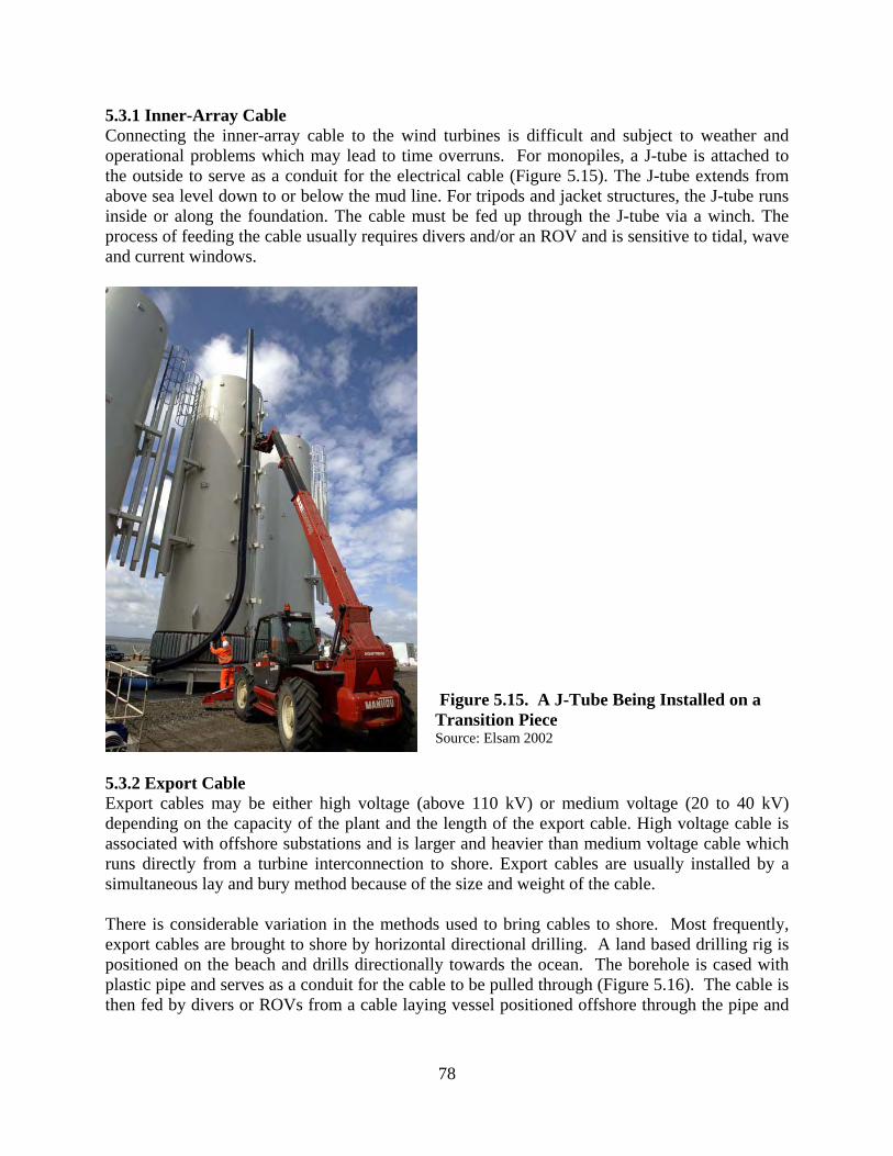
78

5.3.1 Inner-Array Cable Connecting the inner-array cable to the wind turbines is difficult and subject to weather and operational problems which may lead to time overruns. For monopiles, a J-tube is attached to the outside to serve as a conduit for the electrical cable (Figure 5.15). The J-tube extends from above sea level down to or below the mud line. For tripods and jacket structures, the J-tube runs inside or along the foundation. The cable must be fed up through the J-tube via a winch. The process of feeding the cable usually requires divers and/or an ROV and is sensitive to tidal, wave and current windows.

Figure 5.15. A J-Tube Being Installed on a Transition Piece Source: Elsam 2002

5.3.2 Export Cable Export cables may be either high voltage (above 110 kV) or medium voltage (20 to 40 kV) depending on the capacity of the plant and the length of the export cable. High voltage cable is associated with offshore substations and is larger and heavier than medium voltage cable which runs directly from a turbine interconnection to shore. Export cables are usually installed by a simultaneous lay and bury method because of the size and weight of the cable. There is considerable variation in the methods used to bring cables to shore. Most frequently, export cables are brought to shore by horizontal directional drilling. A land based drilling rig is positioned on the beach and drills directionally towards the ocean. The borehole is cased with plastic pipe and serves as a conduit for the cable to be pulled through (Figure 5.16). The cable is then fed by divers or ROVs from a cable laying vessel positioned offshore through the pipe and

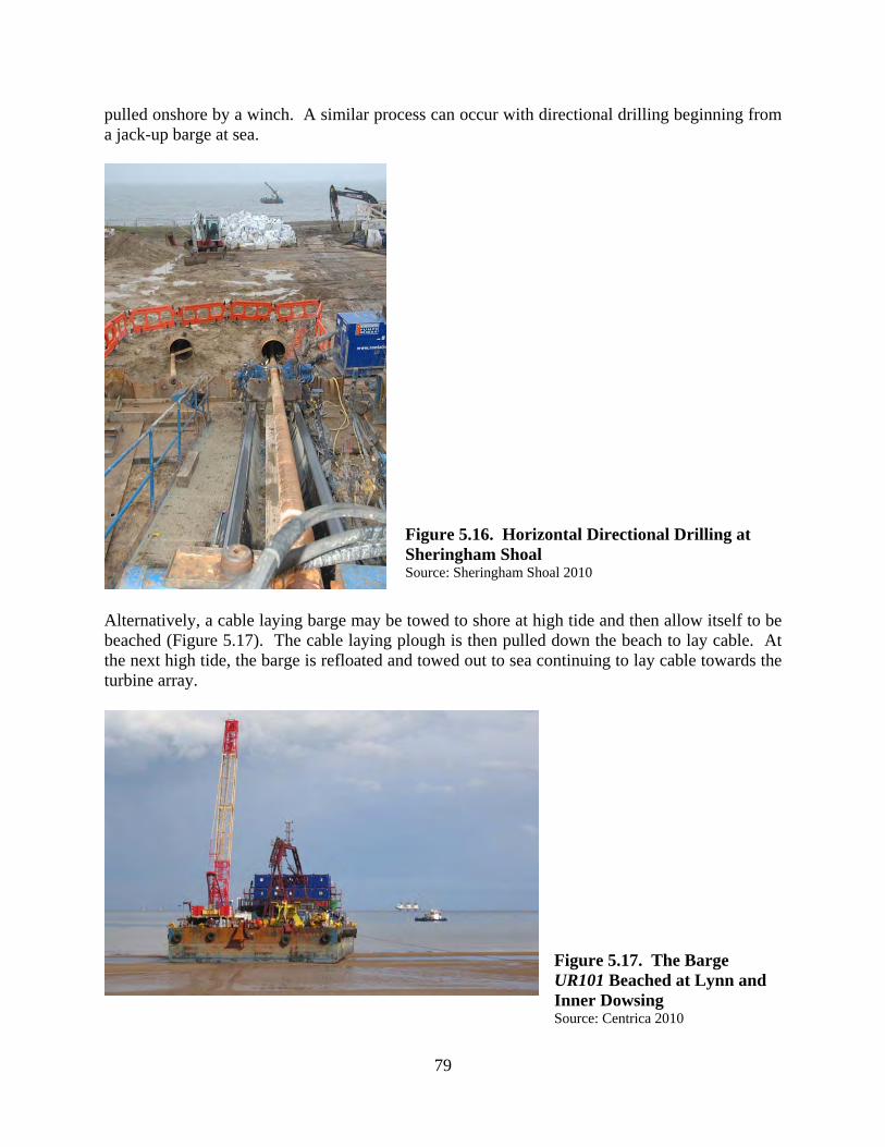
79

pulled onshore by a winch. A similar process can occur with directional drilling beginning from a jack-up barge at sea.

Figure 5.16. Horizontal Directional Drilling at Sheringham Shoal Source: Sheringham Shoal 2010

Alternatively, a cable laying barge may be towed to shore at high tide and then allow itself to be beached (Figure 5.17). The cable laying plough is then pulled down the beach to lay cable. At the next high tide, the barge is refloated and towed out to sea continuing to lay cable towards the turbine array.

Figure 5.17. The Barge UR101 Beached at Lynn and Inner Dowsing Source: Centrica 2010

80

5.3.3 Factors Impacting Installation The time to install inner-array cabling depends on the number of turbines and layout, soil type, depth of burial, and scour protection requirements. The time to install export cable depends on the distance to the onshore substation, soil type, depth of burial, scour protection, and onshore transition. In shallow water, water depth does not play a significant role in installation time. The process of laying cable is affected by the weight and length of the cable. Inter-turbine cables are generally transported and installed in lengths approximately equal to the distance between turbines (usually, less than 800 m), while export cables are at least as long as the distance to shore (3 to 60 km). As a result, a length of inner-array cable may weigh 10 to 20 tons, while an export cable may weigh 500 to 700 tons for a nearshore (10 km) wind farm. The sizes and weights of cable impact the vessels required and the installation time. Burial depth is influenced by soil type, the probability of scour and government regulations. Increases in the required burial depth increase the likelihood of coming into contact with subsurface conditions that are unsuitable for burial. Scour protection may be required to ensure the necessary depth is maintained. The method and vessels used can impact the installation time. Installation is fastest when using dynamically positioned vessels as the mooring spread does not need to be frequently repositioned. If Method 3 is used, the time that the cable laying vessel is required would be short, but the total time to install cables would be long due to the time needed to excavate and fill the trench. Likewise, an ROV operated from a turbine installation vessel might not be the most time-efficient solution, but the fact that it allows a single vessel to complete two jobs simultaneously could make it preferred over alternatives. For export cable, the length of cable installed may impact installation rate, and as length increases, the rate of installation may increase. Cable laying on the seafloor is expected to proceed rapidly, but landfall and connecting to an offshore substation will involve additional time. The time required for landfall and connection is independent of the length and depends on coastline type and the presence of sensitive habitats. 5.3.4 U.S. Cable Installation In the Cape Wind development plan, the inner-array cable will be installed using jet plowing with a support tug and barge. Scour mats and rock armor will require diver support. The export cable will make landfall via a horizontal borehole drilled from the land toward the offshore exit point. A transmission cable will be pulled through the conduits from a pre-excavated pit landward, and a temporary cofferdam will be utilized and backfilled after the operation is complete.

5.4 Substation Installation

Offshore substations are placed on monopile, jacket or gravity foundations. The same foundation used for the turbines may be used or a different foundation applied. Similar installation techniques for foundations are used for the substation foundation and in some cases, the substation foundation is installed at the same time as the rest of the foundations.

81

The transformer is assembled onshore. It may be transported by barge or lifted off the dock by the crane of a heavy lift vessel and transported to site. Once at site, the superstructure is placed on the foundation and secured into place. After the superstructure is secured, a significant amount of finishing work must still be done, however, this does not require significant vessel assistance.

5.5 European Installation Time Statistics

The purpose of this section is to evaluate and synthesize installation experiences of European wind farms. Our objective is to quantify and describe work activity statistics and correlations to inform and baseline future U.S. development. A reference class based on projects of a similar nature is used to compute statistics (see section 5.5.6). 5.5.1 Data Source Table 5.2 shows the primary sources used for installation time data and identify the best published descriptions. Secondary sources and related gray material are not referenced. For some aspects of installation, no information, or poor quality information, was available. For other aspects, detailed and accurate information was available. Installation times are reported across multiple activities and were not normalized for distance to staging area, weather disruptions, and similar events. The unit time statistics include the impact of these factors and are therefore the total time to install the system rather than the time to install any single component. Table 5.2. Sources of Information on Installation Activities at Select Offshore Wind Farms

Wind Farm Sources Horns Rev 2 Lindvig 2009 Horns Rev 1 Elsam 2002 Middelgrunden Larsen et al. 2005*; Sorensen et al. 2002 North Hoyle Carter 2007* Alpha Ventus Alpha Ventus 2010 Nysted Volund et al. 2004; Gerdes et al. 2006 Thornton Bank Gerdes et al. 2006; C-power 2010 Scroby Sands Gerdes et al. 2006; Douglas-Westwood and Ode 2005* Kentish Flats BERR 2007b Lynn & Inner Dowsing Centrica 2010 Barrow BoWind 2008*; BERR 2007a Q7/Princess Amalia De Vries 2007 OWEZ Gerdes et al. 2006; NoordzeeWind 2008* Lillgrund Vattenfall 2010; Jeppsson et al. 2008*

Note: * indicates a particularly detailed description of the installation process 5.5.2 Foundation Table 5.3 summarizes information on the time required to install foundations20 where reliable data were available. Monopile installation, including transit time, weather delays and transition piece placement, takes on average 3.7 days per pile (SD = 2.1). Installation time ranged from 1.8

20 We consider foundations to be composed of the monopile and transition piece.

82

to 8.6 days per foundation. Excluding Arklow (a small, seven turbine project), the average time per foundation decreased to 3.3 days per monopile (SD = 1.5).

Table 5.3. Offshore Wind Farm Installation Requirements – Foundations

Project name Number of major

vessels

Length of time

(months)

Foundation type

Number of foundations

Installation rate (days per foundation)

Middlegrunden 1 2 gravity 20 3 Nysted 1 131 gravity 73 5.3 Thorton 1 1.1 gravity 6 5.5 Lillgrund 1 14 gravity 48 8.8 Sprogo 0.5 gravity 7 2.1 Gravity Average 4.9 Horns Rev 2 1 5.5 mono 92 1.8 North Hoyle 2 4 mono 30 4 (5.5)2 Rhyl Flats 1 3 mono 25 3.6 Scroby Sands 1 3.5 mono 30 3.5 Kentish Flats 1 2 mono 30 2 Lynn & Inner Dowsing 1 8 mono 54 4.4 Barrow 1 7 mono 30 7 Princess Amalia 1 6 mono 60 3 OWEZ 1 4 mono 36 3.3 Horns Rev 1 2 4 mono 80 1.5 (3) 2 Burbo Bank 1 1.8 mono 25 2.2 Robin Rigg 1 mono 60 Arklow 1 2 mono 7 8.6 Monopile Average 3.7 (4.0) Notes: (1) Includes time for dredging which would not require major installation vessels.

(2) Number in parenthesis is boat days per foundation. (3) Boat days for North Hoyle is not twice the time because the two vessels did not operate for the same period of time.

In two cases, monopiles were driven by one vessel and transition pieces were installed by a second vessel. In these cases, it is the number of boat days21 rather than the total time that is the meaningful statistic. After adjusting the total installation time for these cases, the average time increased to 4.0 boat days per foundation (SD = 2.0). Excluding Arklow, average time per foundation was 3.6 boat days per monopile (SD = 2.1). Installation rates as a function of project size is shown in Table 5.4. For 30 foundations or less, 4.6 boat days per foundation is required, which decreases to 3.8 boat days/foundation for 30-60 foundation installations, and 2.6 boat days/foundation when 60 or more foundations were installed. Indications of scale economics are observed. 21 A boat day is one boat used for one day. Two boats used for one day would equal two boat days.

83

Table 5.4. Rate of Foundation Installation by Number of Foundations in Boat Days per

Foundation

Number of Foundations

Installation time (days/foundation)

Number of observations

≤ 30 4.6 7 30 to 60 3.8 2 ≥60 2.6 3

There are only two projects that used jacket or tripod foundations (Beatrice and Alpha Ventus) and both are small scale test projects. It is unlikely that their methods will be replicated on a large scale and are not considered.

Table 5.5. Offshore Wind Farm Installation Requirements – Turbines

Project Number of major vessels

Duration of Installation (months)

Number of turbines

total

Installation rate

(days/turbine)

Installation method

Lillgrund 1 2.5 48 1.6 3 OWEZ 1 3.5 36 2.9 5 Kentish flats 1 4 30 4.0 4 Scroby Sands 1 3 24 3.8 4 Nysted 1 3 72 1.3 3 Horns Rev 1 2 4 80 1.5 (3.0)* 4 Burbo Bank 1 1.5 25 1.8 2 Princess Amalia 2 11 60 5.5 (9.5)* 5 Middlegrunden 2 1.25 20 1.9 (3.8)* 3 North Hoyle 2 3 30 3.0 (6.0)* 4 Alpha Ventus 1 1.5 6 7.5 3 Thornton Bank 2 2.5 6 12.5 (25.0)* 3 Robin Rigg 2 9 60 4.5 (9.0)* 4 Horns Rev 2 1 6 91 2.0 3 Lynn and Inner Dowsing 1 3.5 54 1.9 1 Barrow 1 5 30 5.0 4 Arklow 1 2 7 8.6 3 Average 4.1 (5.7)*

Note: * Number in parenthesis is boat days per foundation. Princess Amalia boat days are not twice the total time because one vessel was not used for much of the project. 5.5.3 Turbine Table 5.5 depicts the time required to install turbines. The average time to install a turbine was 4.1 days (SD = 3.0). In six of the 18 cases, two vessels were employed and so activity time was normalized on a boat day basis. The average time to install a turbine was 5.7 boat days (SD =

84

5.7). When small projects were excluded (Thornton Bank, Alpha Ventus and Arklow), the average dropped to 4.0 days per turbine (SD = 2.6). In some cases, turbines were installed in under 2 days per turbine including at Lynn and Inner Dowsing, Horns Rev 2, Nysted, Lillgrund and Burbo Bank. The relationship between the installation rate and method of installation method is presented in Table 5.6. Methods 1 and 2 required less than 2 boat days per turbine; Methods 3, 4 and 5 were associated with longer average installation times. This trend is unexpected and is likely due to small sample size.

Table 5.6. Rate of Turbine Installation by Installation Method in Boat Days per Turbine

Installation method

Number of observations

Average rate (SD) (days/foundation)

1 1 1.9 2 1 1.8 3 7 7.1 (8.4) 4 6 5.1 (2.2) 5 2 6.2 (4.7) 6 0

Table 5.7 shows the relationship between the installation rate and the total number of turbines installed. A general trend of faster installation with increasing turbine number provides evidence of learning. The sample sizes are too small and the standard deviations are too large, however, to make any definitive statement regarding turbine number and installation time.

Table 5.7. Rate of Turbine Installation by Number of Turbines in Boat Days per Turbine

Number of turbines Number of observations

Average rate (SD) (days/foundation)

<10 3 13.7 (9.8) 10 to 30 6 4.1 (1.4) 31 to 60 5 5.0 (3.9)

>60 3 2.1 (0.9) Table 5.8. Rate of Turbine Installation by Installation Method and Number of Turbines in

Boat Days per Turbine

Installation Method Number of Turbines 1 2 3 4 5 6 ≤ 30 1.8 11.2 4.7 30 to 60 1.9 1.6 2.9 ≥ 60 1.7 6 9.5

85

In Table 5.8, the two-factor interaction between installation method and number of turbines are depicted. The statistical limitations associated with small sample size are compounded when more than one factor is added to analysis because the number of elements within individual categories may not be adequately populated. We cannot draw any useful conclusions from Table 5.8. 5.5.4 Cable Cable can be laid rapidly but the connection points at turbines (through J-tubes) and pull-ins to shore are subject to weather and operational problems. Table 5.9 depicts the total time required to install export and inner-array cables at offshore wind farms and the installation time per km of cable. Export cables were laid at an average rate 0.7 km/day (SD = 0.4) and inner-array cables were laid at an average rate of 0.3 km/day (SD = 0.1). Export cables rates ranged between 0.2 to 1.4 km/day. For inner-array cables, rates ranged from 0.1 to 0.6 km/day.

Table 5.9. Offshore Wind Farm Installation Requirements – Cables

Length (km) Total time (days) Installation rate (km/day)

Project Number of export cables

Export cable

Inner-array cable

Export cable

Inner-array cable

Export cable

Inner-array cable

Middlegrunden 2 3 14 30 0.47 Nysted 1 11 48 Horns Rev 1 1 57 90 0.63 North Hoyle 2 12 15 49 105 0.5 0.14 Scroby Sands 3 4 17 60 60 0.2 0.28 Barrow 1 26 22 130 1501 0.2 0.15 Lillgrund 1 7 22 52 90 1.4 0.24 Robin Rigg 2 13 32 603 1803 0.4 0.18 Alpha Ventus 1 60 16 Thornton Bank 2 36 51 70 161 1.0 0.32 Rhyl Flats 3 11 18 604 90 0.6 0.20 Kentish Flats 3 10 21 30 60 1.0 0.35 Lynn and Inner Dowsing 6 7 19 Princess Amalia 1 28 45 30 150 0.9 0.30 Horns Rev 2 1 42 70 OWEZ 3 15 27 403 903 1.1 0.30 Burbo Bank 3 19 21 Sprogo 5 Average 19 29 0.7 0.3 Notes: 1. Cables laid by ROV while turbine were assembled; therefore includes time for transit by turbine

installation vessel 2. Does not include pre-excavation or delays due to ship damage 3. Planned times 4. Approximate installation times.

These duration estimates are conservative and uncertain. In general, reports of vessel utilization for cable laying are not as common as those for foundation and turbine installation, and so the

86

sample size is smaller. Water depth, distance to port, burial depth22, and scour protection factors are incorporated in the unit time statistics. Table 5.10 shows the installation rate by total cable length for export and inner-array cables. The rates are fairly uniform by type and do not appear to vary significantly with distance. Export cable has a faster lay rate than inner-array cable, likely due to the smaller number of connections that have to be made and reflecting the efficiency of a larger vessel.

Table 5.10. Rate of Cable Installation by Cable Distance in km/Day

Distance (km)

Number of Observations

Average rate (km/day)

<20 4 0.3 (0.1) 20-30 4 0.3 (0.1) 31 to 50 2 0.2 (0.1)

Inner array

>50 2 0.5 (0.2) <20 2 0.8 (0.8) 20 to 30 5 0.6 (0.3)

Export

>30 3 0.9 (0.1) In Table 5.11, export cable installation time by voltage and distance is depicted. Medium voltage cable is smaller and lighter than high voltage cable and has a faster lay rate; further, as distance increases, so does the lay rate, perhaps reflecting learning effects or more efficient operations.

Table 5.11. Export Cable Installation Time by Voltage and Distance

Length (km) High Voltage

(>132 kV) Medium Voltage

(< 36 kV) Average ≤ 30 0.57 0.73 0.66 > 30 0.85 1.00 0.90 Average 0.68 0.78

5.5.5 Substation There is little reliable data on substation installation. The best record of the installation of a substation is from Thanet, where the jacket and substation were installed by the Stanislaw Yudin in four days. The Cape Wind EIS states that installation of its substation will require one month, but much of this time will be spent doing finishing work, and heavy-lift vessel support will only be required for a few days during this time. Foundation installation requires approximately the same amount of time and same vessels required for monopile or jacket installation. From the information in Table 5.3 we would expect a substation monopile foundation to take approximately 4 days for installation, slightly longer if a jacket is used. Placement and securing of the substation could be accomplished in as little as one day. However, since a slow moving heavy lift vessel is required to travel to the site, one or more days would need to be added, depending on the distance to the staging area.

22 For the most part, burial depth falls within a narrow range and is probably undetectable across the sample.

87

5.5.6 Reference Class Statistics The reference class for U.S. offshore installations is defined as follows. First, we consider 100 MW nameplate generation capacity for commercial development. Monopiles are considered the most likely foundation strategy for shallow water (< 30 m) development in U.S. waters and gravity foundations are excluded. We consider installed projects and projects under construction in 2010. Projects built before 2000 are not considered. We consider all contract types and European offshore regions to ensure breadth of coverage. Projects built outside Europe are not considered because of differences in supply chains, labor rates, contract types, and government involvement. Based on the data in Tables 3, 5 and 9, estimated values for shallow water monopile, turbine, inner-array cable, export cable, and substation installation are presented in Table 5.12 for demonstration (≤100 MW, ≤30 turbines) and commercial (>100 MW, >30 turbines) development. In Table 5.13, an alternative reference class for commercial development is provided that is slightly broader and uses more of the existing data set. Here we only excluded wind farms with less than 10 turbines, but for export and inner-array cables, all values were included; test projects (Alpha Ventus and Thornton Bank) were also maintained. The ranges in Table 5.13 are the full range of observed values for installation of each component rather than a function of the standard deviation. In general, using two standard deviations will give similar results, however, the two standard deviations often encompassed zero and occasionally excluded observed results from the upper ranges of installation time. Given the small sample size, we believe using the full range of observed values is the more conservative approach.

Table 5.12. Average Estimated Times Required by Installation Phase and Development Size

Farm Size Installation Duration (boat days)

Capacity Number of turbines

Monopile (days/pile)

Turbine (days/ turbine)

Inner-array Cable (km/day)

Export Cable (km/day)

≤ 100 MW ≤ 30 4.6 7.2 0.26 0.49 > 100MW > 30 3.1 3.9 0.32 0.98

Table 5.13. Summary of Time Estimates for Installation of Wind Farm Components Commercial in Boat Days per Unit

Component Unit Average SD Range Monopile and transition piece Boat days/component 3.6 2.1 1.8–5.5 Tower and turbine Boat days/ component 4.0 2.6 1.3-9.5 Inner-array cable km/day 0.7 0.4 0.2-1.4 Export cable km/day 0.3 0.1 0.2-0.6 Substation Boat days/component 4-10

88

6. INSTALLATION AND VESSEL SPREAD REQUIREMENTS

The purpose of this chapter is to describe the marine vessels required to develop offshore wind farms. Many vessel types and spreads can be utilized across each stage of the installation process, and generally speaking, owners seek the minimum cost at an acceptable risk from the fleet of vessels available to perform the work requirements. In practice, a number of tradeoffs and constraints are involved in selection. We begin by classifying main installation vessels, cable installation vessels, and spread vessels. Main installation vessels are used to install foundations, turbines and substations. Cable installation vessels install inner-array or export cable. Spread vessels support the other two categories through crew and material supply, anchor handling or towing. We discuss factors impacting vessel requirements, selection and activity durations. We also discuss vessel spread composition and size and conclude with a discussion of methods for procuring vessels in the U.S.

6.1 Vessel Categorization

6.1.1 Main Installation Vessels Main installation vessels are grouped according to liftboats, jackup barges, self-propelled installation vessels (SPIV), or heavy lift vessels. Liftboats, jackup barges and SPIVs are collectively referred to as elevating vessels because they elevate above the water line. SPIVs are also frequently called turbine installation vessels (TIV) because they are used almost exclusively for these operations. We use the term turbine installation vessel to refer to any vessel capable of installing turbines or foundations and SPIV as a specific class of TIV. Basic information on the most commonly used European installation vessels are given in Table 6.1. Liftboats Liftboats are self-propelled barge-shaped vessels typically with three legs and a triangular hull. They are usually smaller than other installation vessels and travel between 4 to 6 knots. Liftboats have long legs which allow them to work on high turbines, even with short-boomed cranes (Figure 6.1). Liftboats are not frequently used in Europe but are commonly used for oil and gas construction in the shallow water GOM. Liftboats range in size from small vessels capable of carrying 75 tons and lifting 50 tons to much larger vessels capable of carrying 750 tons and lifting 500 tons. Large liftboats (capable of lifting 200 or more tons with deckloads of at least 500 tons) are capable of carrying one to two turbines23. Jackup Barges Jackup barges are not self-propelled, typically have four legs and range significantly in size. They are usually smaller than liftboats. Figure 6.2 shows a large jackup barge (the Sea Jack) while Figure 6.3 shows a small jackup barge (the JB 114). The Sea Jack has a crane capacity of 800 t and a deck load of 4000 t while the JB 114 has a crane capacity of 280 t and a deck load of 1250 t. Thus, while these vessels are structurally similar, their capabilities are quite different. A small jackup barge may be able to carry two turbines while a large jackup might carry six to

23 Recall that a turbine refers to a collection of components – tower section(s), hub, nacelle, and blades.

89

eight turbines. Depending on tug power, jackup barges would be expected to travel at 4 to 8 knots.

Table 6.1. Vessels Used in Offshore Wind Farm Construction in Europe

Vessel Vessel type Operational water depth

(m)

Max crane capacity (t)

Wind farms

Sea Power SPIV 24 100 Horns Rev 1, Lillgrund, Horns Rev 2 Sea Energy SPIV 24 100 Kentish Flats, Scroby Sands, Nysted,

Princess Amalia, Horns Rev 1 Rambiz Sheerleg crane >100 3,300 Beatrice, Thornton Bank, Nysted Sea Jack Jackup barge 35 1,300 Princess Amalia, Arklow, Scroby Sands Svanen Heavy lift vessel >100 8,700 OWEZ, Rhyl Flats, Gunfleet Sands Titan 2 Liftboat 60 400 Rhyl Flats Buzzard Jackup barge 45 750 Alpha Ventus, Thornton Bank JB 114 and 115 Jackup barge 50 280 Alpha Ventus Thailf Heavy lift vessel >100 14,200 Alpha Ventus Eide Barge 5 Sheerleg crane >100 2,000 Middlegrunden, Nysted, Lillgrund, Sprogo Taklift 4 Sheerleg crane >100 1,600 Alpha Ventus Kraken and Leviathan

SPIV 40 200-300 Walney, Greater Gabbard

Resolution SPIV 35 300 Robin Rigg, Barrow, Kentish Flats, North Hoyle, Lynn and Inner Dowsing

Excalibur Jackup barge 30 220 North Hoyle, Lisa A Jackup barge 50 600 Rhyl Flats MEB JB1 Jackup barge 40 270 Middlegrunden, North Hoyle, Yttre

Stegrund Goliath Jackup barge 50 Up to 1200 Sea Worker Jackup barge 40 400 Robin Rigg; Gunfleet Sands SPIV Self-propelled installation vessels are large self-propelled vessels with four to six legs (Figure 6.4). Most SPIVs are elevating and ship-shaped, however, they may also be column stabilized (e.g. Sea Energy and Sea Power) or barge shaped (Wartsilla TIV). They are distinguished from jackup barges by propulsion and distinguished from liftboats by size and leg number. They have variable deck loads of up to 6,500 t and they travel at 8 to 12 knots. Depending on deck load, deck space and degree of onshore assembly, they could carry ten or more turbines; however, due to onshore assembly, they would be unlikely to carry more than six to eight turbines. Heavy-Lift Heavy-lift vessels are barge-shaped hulls with high capacity cranes; they lack an elevating system, and may or may not be self-propelled (Figure 6.5). They may be dynamic positioned or conventionally moored. Heavy-lift vessels include shearleg cranes, derrick barges, and other floating cranes. They are rarely used to install turbines, but may be used for foundation work, for carrying fully assembled turbines, or for installing substations. They travel at 4 to 8 knots.

90

Figure 6.1. The KS Titan II Liftboat Source: Semco 2010

Figure 6.2. The Sea Jack under Tow Source: DONG Energy 2010b

Figure 6.3. The JB 114, a MSC SEA 2000 Jackup Barge Source: Drydocks World 2010

Figure 6.4. The MV Resolution Working at Barrow Source: BoWind 2008

91

6.1.2 Cable-Laying Vessels Cable-laying vessels are used to lay the power cable between turbines and to shore. Export cable laying vessels are large barges or self-propelled vessels dedicated specifically for cable laying operations (Figure 6.6). These vessels typically have a turntable capable of spooling over 1000 tons (typically approximately 5,000 t, or approximately 100 km) of cable and may operate a cable laying plow or ROV. Inner-array cables may be laid by a variety of vessels, and because the size of the cable and the distance between connection points is considerably smaller than export distances, the vessel requirements are less demanding and may be installed with a modified supply vessel (Figures 6.7, 6.8). Modified offshore supply vessels are typically dynamically positioned and capable of operating a cable laying ROV24 or plow. However, it is also common for the main installation vessel and the export cable vessel to be employed in inner-cable laying.

Figure 6.5. The Heavy Lift Vessel Rambiz Installing a Turbine at the Beatrice Project Source: Talisman Energy 2008

Figure 6.6. The Eide 28, an Export Cable Laying Vessel Source: VSMC 2010

24 The ROV may carry a spool of cable itself or may be supplied with cable by the installation vessel.

92

Figure 6.7. The Nico, a Modified Offshore Supply Vessel Installing Inner-Array Cable Source: DONG Energy 2009c

Figure 6.8. The Polar Prince, another Cable Laying Vessel Source: Troll Windpower 2009 6.1.3 Vessel Spreads Support vessels are required for all installation stages but the size and composition of the support spread will vary over the course of installation depending on the capability of the main installation vessel and the scope of work. There are several classes of spread vessels used in offshore wind installations including crewboats, multicats, tugs, dive support vessels, dredging/scour vessels and other vessels. Crewboats (also called wind farm support vessels) are 10 to 25 m long and carry between 10 to 15 people. They range from small rigid hulled inflatable boats (RIBs; Figure 6.9) to 20 m catamarans. In addition to their personnel transfer role, RIBs are often used as utility vessels for energizing turbines, enforcing safety zones, conducting environmental studies, or supporting shallow water divers.

93

Figure 6.9. A Rigid Hull Inflatable Boat Used for Personnel Transfer and Utility Work at Gunfleet Sands Source: DONG Energy 2009c Multicats are multipurpose vessels, typically 12 to 30 m in length and usually equipped with a small (under 50 t) crane and a large open deck (Figure 6.10). They are primarily used for anchor handling and may be used for light transport duties, diver support, and other tasks. Multicats are not common in the U.S.

Figure 6.10. The Forth Jouster, a 26 m Multicat Source: DONG Energy 2009c Dive support can be conducted from a variety of vessels with minor modifications. Dive support vessels provide a place to launch, supply, communicate with and recover shallow water divers; they are much smaller than vessels used in the offshore oil and gas industry as the divers operate at shallow water and do not require saturation equipment.

94

Dredging and scour protection vessels are highly variable depending on the application. In their simplest form they may consist of a backhoe excavator placed on a spud barge. More sophisticated dynamically positioned trailing suction hopper dredges are also used for gravity foundations. Scour protection is typically placed by a side dumping barge but could also be placed by a utility vessel. Ocean going tugs are used to tow deck barges and non self-propelled vessels from the shore base to the offshore site. In many cases they are equipped with a small crane for anchor handling. These vessels are typically 1500 to 5000 hp.

6.2 Factors Impacting Vessel Selection

Vessels are matched with projects based on economic and technical factors. Technical demands depend on the stage of installation. Requirements for foundation installation are different than for turbine and cable installation. 6.2.1 Foundation Foundations may be installed by any main installation vessel, but are less likely to be installed by liftboats due to their low crane capacity (Table 6.2). Important factors in foundation installation are crane capacity and water depth. In some cases, vessels with crane capacities below the foundation weight may be used in combination with specialized pile gripping devices or monopiles may be floated to site. In shallow areas, water depth can limit the choice of vessel and barge shaped hulls may be preferred. Crane lift height is usually not an important factor because foundations only need to clear the vessel deck. Transit speed is also not critical because there are alternative methods for foundation transport that do not require the installation vessel to move back and forth from port.

Table 6.2. Vessel Capabilities by Work Type

Installation Activity Vessel Class Foundation Turbine Cable Substation Liftboat U Y N N Jackup barge Y Y N Y SPIV Y Y Y Y Heavy lift Y U N Y Note: U is unlikely 6.2.2 Turbine Turbines may be installed by any main installation vessel, but are less likely to be installed by heavy-lift vessels due to the height and sensitive nature of the lifts (Table 6.2). Heavy-lift vessels are capable of installing completely assembled turbines. Important factors in turbine installation are variable load, crane specification and deck space. Variable load dictates the weight of turbine components carried per trip. Crane height and leg length determine if a vessel can install turbines at a given hub height. Crane lift capacity determines the number of lifts required per turbine and sets limits on the degree of onshore

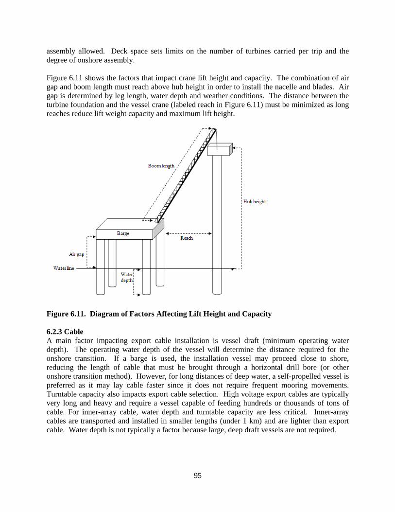
95

assembly allowed. Deck space sets limits on the number of turbines carried per trip and the degree of onshore assembly. Figure 6.11 shows the factors that impact crane lift height and capacity. The combination of air gap and boom length must reach above hub height in order to install the nacelle and blades. Air gap is determined by leg length, water depth and weather conditions. The distance between the turbine foundation and the vessel crane (labeled reach in Figure 6.11) must be minimized as long reaches reduce lift weight capacity and maximum lift height.

Figure 6.11. Diagram of Factors Affecting Lift Height and Capacity 6.2.3 Cable A main factor impacting export cable installation is vessel draft (minimum operating water depth). The operating water depth of the vessel will determine the distance required for the onshore transition. If a barge is used, the installation vessel may proceed close to shore, reducing the length of cable that must be brought through a horizontal drill bore (or other onshore transition method). However, for long distances of deep water, a self-propelled vessel is preferred as it may lay cable faster since it does not require frequent mooring movements. Turntable capacity also impacts export cable selection. High voltage export cables are typically very long and heavy and require a vessel capable of feeding hundreds or thousands of tons of cable. For inner-array cable, water depth and turntable capacity are less critical. Inner-array cables are transported and installed in smaller lengths (under 1 km) and are lighter than export cable. Water depth is not typically a factor because large, deep draft vessels are not required.

96

6.2.4 Substation Substation topsides typically weigh 500 to 2000 tons. The installation vessel must have the crane capacity to lift the substation. Lift height is usually not critical as substations are generally not tall, however, if a substation needed to be elevated significantly due to potential wave heights, lift height could be a factor, especially for shear-leg cranes. To date, substations have been installed by heavy-lift vessels; as crane capacity of jackup barges and liftboats increases, they could be used to install substations.

6.3 Support Spread Size and Composition

The required spread depends on the specifications of the vessels used, the installation procedures, environmental conditions, safety regulations and the size of the project. Several potential spreads required to support main installation vessels are shown in Table 6.3. In all cases, jackup barges will require one tug for propulsion, while SPIVs and liftboats will not. Jackup barges will require some vessels for anchor handling. It is possible that liftboats or SPIVs would need anchor handling, however, we consider this unlikely. For general navigational purposes, jackups are likely to require one tug and one crew/utility vessel. SPIVs and liftboats will usually require one crew/utility vessel.

Table 6.3. Estimated Potential Spreads by Vessel Type and Activity

Number of tugs

Number of barges

Number of utility/crew boats

Vessel type Component Transport system min max min max min max SPIV Foundations Barge/float 2 3 0 3 2 4 SPIV Foundations Self-carry 0 0 0 0 1 3 SPIV Turbines Self-carry 0 0 0 0 1 3 Jackup Foundations Barge/float 3 4 0 3 2 4 Jackup Foundations Self-carry 1 2 0 0 1 3 Jackup Turbines Self-carry 1 2 0 0 1 3 Liftboat Turbines Self-carry 0 0 0 0 1 3 6.3.1 Foundations In addition to general navigation and support, spreads are required for transporting supplies. Foundations may be carried by the installation vessel, barged to the site, or floated. If the installation vessel carries the foundations, no additional spread vessels are needed. If the foundations are barged, two tugs and two barges will be needed to ensure a constant supply of foundations to the offshore site. If the foundations are floated, two tugs would be required. While monopiles may be floated, transition pieces are not; they could be carried by the installation vessel or barged. Therefore, in most cases, zero to two tugs and barges are required for foundation supply. 6.3.2 Turbines Turbine components are most likely to be carried by the installation vessel and would not require additional vessel support. If components are carried by a feeder vessel, it is highly likely that such a vessel would be self-elevating and/or dynamically positioned. A barge pulled by a tug is unlikely to allow for safe turbine transfers at sea. Therefore, a turbine feeder system would

97

require the addition of another main installation vessel rather than the addition of tugs, barges, or crew/utility vessels. 6.3.3 Cable Cable laying vessels also require spreads. Both self-propelled and non-self-propelled vessels require at least one general purpose crew/utility vessel and one dive support vessel or other support vessel. Additionally a non-self-propelled vessel requires tugs for propulsion and anchor handling. Due to the frequency of mooring positioning and the number of mooring lines, at least two tugs are likely required. 6.3.4 Example European Spreads Figures 6.12 and 6.13 show the number of vessels on site by week for the Thanet and Gunfleet Sands developments. In each case, weekly notices to stakeholders were released detailing the activities and vessels on site. Both wind farms are UK commercial sized projects (172 and 300 MW for Gunfleet and Thanet, respectively) developed in the 2009-2010 period. Both are built on monopile foundations. Gunfleet Sands is 7 km from shore and developed by DONG, Thanet is 12 km offshore and developed by Vattenfall. Perhaps the most significant difference is that Thanet contains 100, 3 MW turbines while Gunfleet Sands contains 48, 3.6 MW turbines. The minimum spread at Thanet is one main installation vessel (in this case the non-self propelled Sea Jack), two crewboats, two tugs and one other vessel. When a second installation vessel was added (the self-propelled Resolution) the spread increased to four tugs, two crewboats, and one guard vessel, however, one of these tugs was often used to move supply barges on inland waterways. As cable laying began in week 27, the number of multicats and crewboats increased. The maximum number of vessels operating at any one time was 32; this occurred when two jack-ups, three cable lay vessels and one heavy-lift ship were all on site.

Figure 6.12. The Spread at Thanet Windfarm by Week Source: Vattenfall

98

At Gunfleet Sands (Figure 6.13), despite a smaller number of turbines, a larger spread was often used. The minimum number of vessels operating at one time was twelve. Typically, the spread consists of one self-propelled main installation vessel (the Titan 2), one tug towing one barge, one cable laying catamaran, two to three multicats with at least one supporting cable laying and one supporting the installation vessel, approximately 10 crewboats and at least 3 other vessels. We calculated the average number of support vessels per construction vessel for Thanet and Gunfleet Sands. Multicats, crewboats, barges, tugs, diving support and other vessels were considered as support vessels and main installation vessels, cable laying vessels and dredging/scour vessels were considered as construction vessels. At Thanet the average number of support vessels per construction vessel was 3.9; at Gunfleet Sands the average was 6.6. These data are further classified by support vessel type in Table 6.4. The data show significant variation in the total number of vessels required for support as well as variance in the types of vessels used.

Figure 6.13. The Spread at Gunfleet Sands Offshore Wind Farm by Week Source: Gunfleet Sands Notice to Mariners

Table 6.4. Average Number of Support Vessels Required per Construction Vessel at Thanet and Gunfleet Sands

99

Vessel Type Thanet Gunfleet Sands Crew 1.3 3.2 Tug 1.6 0.9 Mulitcat 0.2 1 All Others 0.7 1.5 Total 3.9 6.6

6.3.5 Potential U.S. Spreads The utilization of barges, tugs, and small crewboats (RIBs) is unlikely to differ in the U.S. and Europe. However, due to the availability of some vessel types, U.S. spreads may differ from European spreads. Multicats are unlikely to be used in the U.S. because they are not common. Instead, small utility boats similar to those used in the GOM oil and gas industry could be employed for anchor handling, dive support, commissioning, and other activities. In Europe, most crewboats are smaller than those used in the GOM oil and gas industry. Small crewboats from the GOM oil and gas industry could be used, or more specialized vessel could be newbuilt in local shipyards. Such specialized vessels may allow for safer crew transfers. There are a large number of dynamically positioned offshore supply vessels in the GOM which could be mobilized to wind farm sites. These vessels could be used to shuttle wind farm components from shorebases to offshore wind facilities25. This would allow for the use of smaller vessels (such as liftboats) to be used for turbine installation, and could eliminate the need for some barges and tugs.

6.4 U.S. Vessel Procurement

Main installation vessels may be procured for the U.S. offshore wind market by moving vessels from other U.S. industries or newbuilding. Vessels could also be mobilized from Europe, but high level of European activity and the requirements of the Jones Act will constrain the European fleet. 6.4.1 Jones Act The Jones Act (the Merchant Marine Act of 1920) requires that all commerce between two U.S. ports be carried on a U.S. flagged, crewed and owned vessel. The definition of a port includes any area on the OCS. The Jones Act is enforced by the Customs and Border Protection (CBP) Agency and the Maritime Administration (MARAD). There are several activities that are excluded from the Jones Act via administrative policy developed by CBP as well as activities exempted from the Jones Act under specified circumstances. Customs and Border Protection CBP is tasked with determining when vessels are engaged in coastwise transport and subject to the provisions of the Jones Act. For the past several decades, CBP has promulgated a liberal definition of “vessel equipment”, which is not subject to the provisions of the Jones Act. In general, the CBP has allowed non-U.S. vessels to carry merchandise (typically pipelines, 25 For example, the Hornbeck 250 class OSVs are dynamically positioned, have 185 x 45 ft decks, cruise at 10 knots and can carry over 2000 t of deck load. The typical duty of these vessels involves dynamically positioning next to a stationary rig or platform and offloading cargo. This is similar to the process that would be required to supply turbine installation vessels.

100

jumpers, risers, and umbilicals) from a U.S. port to a location on the OCS as long as the same vessel installed the merchandise. CBP has allowed non-U.S. liftboats to transport and install equipment including decks, generators, jackets, boat landings and related equipment from U.S. ports to locations on the OCS. In these cases, the CBP has ruled that the material being carried is not merchandise but vessel equipment as it is required for the vessel to perform its intended “mission”. In July 2009, CBP issued a decision which would restrict the definition of vessel equipment. According to CBP, the definition of equipment as codified in the Tariff Act of 1930 is “portable articles necessary and appropriate for the navigation, operation or maintenance of the vessel and for the comfort and safety of the persons on board.” This definition does not reference the mission of the vessel. Material such as pipelines, wellheads, or platform decks were deemed unnecessary for the navigation, operation or maintenance of the vessel and CBP’s previous enforcement of the Jones Act was deemed to be contrary to the legislative intent. As a result, CBP revoked numerous rulings allowing foreign pipelaying vessels and liftboats to operate in coastwise trade (Ressin 2009). In October 2009, the CBP withdrew its July decision revoking its previous rulemaking citing a significant public response on both sides of the issue. They indicated that new policy would be announced in the near future (Quillen 2010). In separate rulings independent of the definition of vessel equipment, the CBP allows non-U.S. crane vessels to lift and install jackets and other structures on the OCS, provided the crane does the movement, not the vessel itself. The CBP also allows the transport of material from a U.S. port to a location on the OCS as long as the location on the OCS is a dynamically positioned vessel (CBP 2010). MARAD Independently, MARAD manages exemptions to the Jones Act. These are separate from CBP’s rulemaking and involve vessels that are deemed to be engaged in coastwise transport. There are two classes of vessels that may be granted exemptions26: small passenger vessels and barges and other vessels used in the offshore petroleum industry. Small passenger vessels capable of carrying up to twelve people and over three years old may be granted exemptions. Vessels must be greater than 5 net tons (approximately 24 feet), must be owned by a U.S. citizen and may not carry cargo. The launch barge program allows for the use of foreign vessels to transport platform jackets offshore if no suitable U.S. vessel is available. The program applies to any vessel capable of loading, transporting and launching, or installing a jacket. It is limited to the offshore oil industry. Relevance to Offshore Wind Under existing rulemaking, the Jones Act may not apply to turbine or foundation installation. Turbine and foundation installation is similar to a liftboat carrying and installing a deck on an offshore jacket. Cable installation is similar to pipelaying. Under current rulings, the only vessels that would need to comply with the Jones Act would likely be barges and tugs. However, CBPs interpretation of what constitutes vessel equipment is under review and it is possible that the definition will be tightened to exclude foreign turbine installation vessels or cable installation vessels from transporting wind farm components. 26 Additionally, exemptions may be granted for national defense or in emergencies.

101

6.4.2 U.S. Fleet Circa 2010 We compiled a list of U.S. vessels capable of contributing to the construction of offshore wind farms. We assume that an elevating vessel must have a crane capacity of at least 200 tons to be potentially useful27. Further, we assume that any non-elevating crane vessel with a lift capacity greater than 500 tons is also potentially useful, especially for placing foundations and offshore transformer stations and driving monopiles. There are a limited number of vessels currently working in the U.S. capable of installing offshore wind turbines (Tables 6.5 and 6.6). Most of these vessels are in the GOM offshore oil and gas industry, although some are used for marine salvage or in civil construction. We do not consider conversions of existing vessels nor do we consider derrick barge/pipe lay vessels or semisubmersible vessels with extreme lifting capacity28. Table 6.5. Elevating Vessels Active in the U.S. and/or with U.S. Flags Capable of Offshore

Wind Farm Construction

Name Owner Vessel type Crane capacity (short t)

Water depth

capacity (m)

Max hook height (ft)

Deck load

(short t)

2009 Dayrate estimate (1000 $)

Superior Influence Superior Lift boat 200 60 120 750 30 Superior Respect Superior Lift boat 200 60 120 750 30 Superior Storm Superior Lift boat 250 55 100 500 30 Superior Gale Superior Lift boat 250 55 100 500 30 Superior Champion Superior Lift boat 200 55 100 500 30 Jacob CS Liftboats Lift boat 200 60 130 450 38 Mammoth Elevator EBI Lift boat 400 50 150 300 Karlissa A Titan Jack up barge 300 50 180 1000 25 Karlissa B Titan Jack up barge 300 50 180 1000 25

Source: personal communication with company personnel Based on the information in Table 6.6, it seems likely that there is sufficient U.S. non-elevating heavy-lift capacity; there are a large number of derrick barges and shear leg cranes available in the U.S. However, there are a relatively small number of elevating vessels capable of installing offshore wind turbines and those that do exist are not particularly well suited to this task. The large liftboats, for example, the Superior Storm or Superior Respect are potentially capable of lifting rotors and nacelles to 70 m, especially in shallow water. However, they only have 500 to 750 t variable deck loads and would have difficulty carrying more than one or two, 3 to 3.6 MW turbines at a time. Tables 6.5 and 6.6 also give 2009 dayrates from the oil and gas or marine construction industries. These rates are vessel-only spot rates and do not include spreads. Contract terms, durations and dayrates are likely to be different in the offshore wind sector.

27 Liftboats with crane capacities of 150 tons would limit the type of offshore turbine used to less than 3 MW. 28 We do not consider derrick/barge pipelay vessels or semisubmersible heavy-lift vessels because their capabilities and cost exceed those required for wind applications.

102

Table 6.6. Non-Elevating Vessels Active in the U.S. or with a U.S. Flag Capable of Offshore Wind Farm Construction

Name Owner Vessel type Crane

capacity (short t)

Max hook height (ft)

Dayrate estimate,

2009 (1000 $)

Location

Lili Bisso Bisso Marine Shear leg 600 200 GOM Cappy Bisso Bisso Marine Shear leg 700 155 GOM Big T T&T Marine Shear leg 600 150 GOM Mr 2 Hooks Laredo Shear leg 800 110 50 GOM Illuminator Laredo Shear leg 513 130 50 GOM IOS 800 International Shear leg 800 175 75-100 GOM Chesapeake DonJon Shear leg 1000 230 Atlantic Left Coast Lifter American Bridge-

Flour Shear leg 1700 328 NA* Pacific

Taklift 1 Smit Shear leg 800 260 GOM Titan II Global Industries Crane vessel 880 206 GOM William Kallop Offshore Specialty Derrick barge 1750 272 150 GOM Superior Performance

Superior Derrick barge 880 170 80 GOM

Raeford Offshore Specialty Derrick barge 700 205 GOM Swing Thompson Offshore Specialty Derrick barge 1320 206 150 GOM Superior Pride Superior Derrick barge 880 170 67.5 GOM DB 16 J Ray McDermott Derrick barge 600 231 GOM DB 50 J Ray McDermott Derrick barge 4400 262 350-500 GOM Atlantic Horizon Caldive Derrick barge 500 205 GOM Pacific Horizon Caldive Derrick barge 700 213 GOM DB General General Const. Derrick barge 700 200 96 Pacific EP Paup Manson Derrick barge 1000 210 139 GOM Wotan Manson Derrick barge 500 115 Pacific Arapaho Tetra Derrick barge 800 200 150 GOM DB 1 Tetra Derrick barge 615 200 150 GOM Source: personal communication with company personnel. Note: * Left Coast lifter was built for the construction of the Bay Bridge in CA by the developers. Building costs were approximately $50 million and it has never been used on a dayrate chartered contract. 6.4.3 Newbuilding Table 6.7 shows the specifications of the most popular newbuild designs. Vessels may be elevating, dynamically positioned or conventionally moored, they may be self-propelled or towed, they may have lift capacities from 100 to 5,000 t or more and they may have variable loads of 500 to 4,000 t or more. All new building for the wind industry is currently composed of elevating vessels. Among the most frequent European newbuild designs are the SEA 2000 and the NG 9000. These two vessel designs differ in their capabilities and represent two alternative methods for

103

turbine installation; the SEA 2000 is relatively small, inexpensive jackup barge while the NG 9000 is a large, expensive SPIV. The SEA 2000 (Figure 6.3) has a 55.5 m long by 32.2 m wide hull with a variable load of 1,600 t. It can be equipped with a 1200 t crane. The 2009 costs for a newbuilt SEA 2000 was about $60 to $65 million. The NG is 130.8 m long and 39 m. It is ship-shaped, self-propelled, dynamically positioned and capable of 12 knots. It is equipped with an 800 t crane, has a variable load of 6,500 t and a deck area of 3,200 m2. A NG 9000 costs about $160 million to build. Either vessel would be capable of installing turbines and monopiles, but would differ in spread requirements, and overall work durations. There are several shipyards in the U.S. capable of building self-propelled turbine installation vessels and several others capable of building large turbine installation barges. Table 6.8 shows the shipyards most likely to build turbine installation vessels or barges. Shipyards were included if they delivered a large OSV, a large, deep draft vessel (excluding naval vessels), a liftboat, or an oceangoing barge in the past two years (Colton 2010).

Table 6.7. Specification of Newbuild Designs

Design Water depth (m)

Number of legs

Crane capacity (t)

Total number built and under build

Variable load (t)

Self propelled speed (kn)

MC NG 9000 45 4 800 3 6500 12 MSC SEA 2000 40 4 1200 4 1600 NA MSC SEA 2750 45 4 1 3000 NA MSC SEA 3250 45 4 1 3800 NA MSC NG 7500 40 6 1000 2 6000 12 MSC NG 2500 52 4 300 2 1300 8 MSC NG 5300 45 4 500 1 2600 8 Semco 280 50 3 400 1 500 NA Wartsila 50 4 800 0* 4100 6 Note: *Three are planned for construction but not under build

104

Table 6.8. U.S. Commercial Shipbuilders Capable of Building Turbine Installation Vessels

Builder Typical Vessels Location Aker Philadelphia Product carrier Philadelphia PA Atlantic Marine OSV AL &FL Bay Shipbuilding Barge Sturgeon Bay WI Signal (Bender) Rig, OSV MS, TX, AL Boconco Liftboat Bayou La Batre AL Bollinger Barge, OSV Amelia; Lockport LA Candies Shipbuilding OSV Houma LA Conrad Industries Liftboat Morgan City Corn Island Shipyard Barge Lamar IN Dakota Creek Industries OSV Anacortes WA Eastern Shipbuilding OSV, Barge Panama City FL Elevating Boats, Inc. Liftboat Laffite LA GD NASSCO Product carrier San Diego Gunderson Marine Barge Portland OR Halimar Shipyard Liftboat, OSV Morgan City LA Keppel AMFELS Rig Brownsville TX Le Tourneau Rig Vicksburg MS Leevac Industries OSV Jennings LA North American Sbldrs. OSV Larose LA Quality Shipyard OSV Houma LA Rodriguez Boatbuilders Liftboat Bayou La Batre AL SENESCO Barges North Kingstown RI Thoma-Sea Shipbuilders OSV Lockport LA US Barge Barge Portland OR VT Halter Marine RV, Barge, OSV MS Zidell Marine Barge Portland OR Semco Liftboat Laffite LA

Source: Colton (2010)

105

7. MODELLING INSTALLATION VESSEL DAYRATES

The costs to a U.S. developer to lease an installation vessel are subject to a large degree of uncertainty due to supply-demand conditions, willingness to pay, and regulatory requirements. European dayrates are not widely reported and are unlikely to be reflective of U.S. cost due to the strong competition for vessels in Europe and the manner in which installation services are provided. Dayrates for liftboats in the U.S. GOM are transparent and widely reported, and these vessels may be used for wind development, but once the vessels leave their operating region the cost dynamics will change. Developers may decide to build a new vessel for wind installation but the costs and risks of the lease vs. own decision option varies widely. The purpose of this chapter is to estimate ranges for vessel dayrates for U.S. offshore wind installation. We begin with anecdotal information on European dayrates and discuss cost trends in the Gulf of Mexico market. We then estimate vessel dayrates using three model frameworks: dayrate components, by assuming dayrates are a percentage of vessel capital costs, and by constructing a model for a developer-owned vessel. Mobilization costs are estimated and parameterized to create estimates of total costs by vessel type and mobilization distance. We conclude with the algebraic development of the models. This material is of a specialized nature and the reader may wish to skim it over lightly on first reading or return to it at a later time.

7.1 European Installation Vessel Costs

Dayrates for similar vessels operating in different regions will differ due to local supply and demand conditions, willingness to pay, and regulatory structure. There is anecdotal information on European installation vessel data that serve as a comparison for the U.S. market. In 2009, SeaJacks signed contracts for the installation of wind turbines at Walney and Greater Gabbard. Both contracts were for approximately 15 months duration and used identical newly built SPIVs (Kraken and Leviathan). Effective dayrates were computed by dividing the value of the contract by the number of days of operation, yielding $148,000 and $176,000 (excluding mobilization costs). In late 2008 and early 2009, Master Marine signed contracts for the Service Jack and Service Jack 2. Both vessels are newbuilt SPIVs. The Service Jack contract was for three years with Conoco Phillips (serving as an accommodation platform); the Service Jack 2 contract was for nine months installing turbines at Sheringham Shoal. The effective dayrates are estimated to be $330,000 and $380,000. Both vessel are large (110 m long and 50 m wide) and capable of operating in deep water (300 ft). Conversations with several vessel brokers and published information (Morgan et al., 2003; Durnford-Slater, Pers. Comm) indicate that elevating installation vessel dayrates typically range from approximately $50,000 to $150,000 depending on the capabilities of the vessel.

106

7.2 Gulf of Mexico Market Trends

The cost to build a vessel and the dayrates that the owner realizes are market-based and independent. Historically, the capital expenditures on newbuilds were amortized over the life of the asset and a designated utilization rate was used to set vessel dayrates. In competitive markets, dayrates change with changes in supply and demand and changes in operating costs caused by increased fuel prices. 7.2.1 Liftboat Dayrates Figure 7.1 shows the average spot liftboat dayrates from 2004 through 2010 for vessels owned by Superior Energy Services operating in the GOM. The 5-year average dayrate for the 230-245 class29 liftboats was $23,600 (SD = $5,700) and the average dayrate for 250 class vessels was $31,200 (SD = $7,800). Dayrates for 265 class vessels were slightly higher, on average $37,500 (SD = $3,400). The cost differential in vessel classes reflects the water depth capabilities and variable load and the market demand. Over time, there is significant variability in dayrates. A two standard deviation interval for the 230-245 class yields a range of [$12,220-$35,000] and for the 250 class [$15,600-$46,800].

Figure 7.1. Average Large Liftboat Dayrates in the Gulf of Mexico Source: Superior Energy quarterly reports 7.2.2 Jackup Rig Dayrates Jackup rigs are used for drilling and dayrates are well documented throughout the world's offshore regions. Figure 7.2 shows the GOM average dayrate by water depth. The average dayrate from 2005 to 2009 was approximately $86,000 (SD = $38,000) for rigs capable of operating in 300 ft water depth and $107,000 (SD = $41,000) for larger rigs. Individual dayrates are highly variable; among operating jackups in 2009, for example, dayrates ranged from $28,000 to $398,000. While jackups rigs are somewhat similar to the vessels required for

29 Class indicates leg length (in ft) and is approximately 50 to 70 ft greater than maximum operating water depth.

107

offshore wind development in terms of capital costs and conceptual design, they are used very differently and will have different dayrates.

Figure 7.2. Average Jackup Dayrates in the Gulf of Mexico Source: Bailey et al. 2010

Figure 7.3. Average OSV dayrates in the Gulf of Mexico Source: Workboat 2002-2010

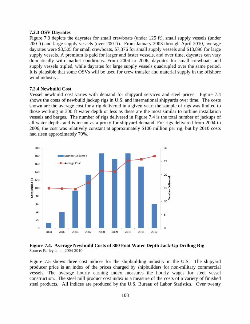
108

7.2.3 OSV Dayrates Figure 7.3 depicts the dayrates for small crewboats (under 125 ft), small supply vessels (under 200 ft) and large supply vessels (over 200 ft). From January 2003 through April 2010, average dayrates were $3,505 for small crewboats, $7,376 for small supply vessels and $13,898 for large supply vessels. A premium is paid for larger and faster vessels, and over time, dayrates can vary dramatically with market conditions. From 2004 to 2006, dayrates for small crewboats and supply vessels tripled, while dayrates for large supply vessels quadrupled over the same period. It is plausible that some OSVs will be used for crew transfer and material supply in the offshore wind industry. 7.2.4 Newbuild Cost Vessel newbuild cost varies with demand for shipyard services and steel prices. Figure 7.4 shows the costs of newbuild jackup rigs in U.S. and international shipyards over time. The costs shown are the average cost for a rig delivered in a given year; the sample of rigs was limited to those working in 300 ft water depth or less as these are the most similar to turbine installation vessels and barges. The number of rigs delivered in Figure 7.4 is the total number of jackups of all water depths and is meant as a proxy for shipyard demand. For rigs delivered from 2004 to 2006, the cost was relatively constant at approximately $100 million per rig, but by 2010 costs had risen approximately 70%.

Figure 7.4. Average Newbuild Costs of 300 Foot Water Depth Jack-Up Drilling Rig Source: Bailey et al., 2004-2010 Figure 7.5 shows three cost indices for the shipbuilding industry in the U.S. The shipyard producer price is an index of the prices charged by shipbuilders for non-military commercial vessels. The average hourly earning index measures the hourly wages for steel vessel construction. The steel mill product cost index is a measure of the costs of a variety of finished steel products. All indices are produced by the U.S. Bureau of Labor Statistics. Over twenty

109

years, the costs charged by shipyards have nearly tripled while the cost of labor has approximately doubled. The cost of steel is more variable but has generally increased.

Figure 7.5. Shipbuilding Price and Earnings Cost Indices Source: Bureau of Labor Statistics 2010

7.3 Dayrate Components

Dayrates are composed of vessel operating expenses, principal and interest payments on debt, and returns on investments (ROI). Estimates of operating costs, finance costs, and ROI for potential U.S. offshore wind installation vessels can be made based on similar marine vessels; summing these components provides an estimate of the dayrate. 7.3.1 Operating Expenses Operating expenses denote all costs borne by a vessel operator beyond capital expenditures. The primary components of operating expense are personnel, fuel cost, insurance, and administrative costs. Vessel type and size determine operating expense. Typical operating expenses for liftboats, jackups, and OSVs in the GOM for 2009-2010 are shown in Table 7.1. The values in Table 7.1 are derived by dividing the annual costs of operation by the number of operating days. In general, operating expenses range between 40 to 65% of dayrates and vary from 5,000 $/day for small liftboats to 40,000 $/day for large drilling rigs. For wind installation vessels, operation expenses will likely lie within the range in Table 7.1. Operating expenses for turbine installation vessels are unlikely to fall below the operating expenses of liftboats because this is an average fleet cost that includes both large and small vessels. Operating expenses are also unlikely to be above the operating costs of jackup rigs, as they are one of the most energy and labor intensive vessels in the market. The size and complexity of the installation vessel will determine where within this range operating expenses fall.

110

Table 7.1. Operating Expenses for Selected Commercial Vessels in the Gulf of Mexico (2009-2010)

Vessel Type Source Daily OpEx

($1000) OpEx as a percentage of dayrate

Jackup Jayaram and Royes 2009 32-40 42-58 Liftboat Hercules 2010; Superior 2010 5-13 62-64 OSV Hornbeck, 2010; Tidewater 2009 6-10 45-48

Operational expenses in dayrate contracts may be divided between the vessel owner and the client. For example, the vessel owner may pay crew expenses and maintenance costs while the client pays for fuel. From the perspective of the wind developer, it is the total operational expense rather than the operational expense included in the contract that is important. As a result, using reported operating expenses for liftboats and jackups likely underestimates the real operating expense to the developer. 7.3.2 Returns on Investment Jayaram and Royes (2009) analyzed financial information of large international drilling rig operators from 1996 to 2008. They used the ratio of EBITDA30 to replacement cost to derive an annual average ROI estimate. Over the study period, ROI ranged from approximately 4 to 14% and averaged 8.5%. Using data from the annual financial fillings of two large, publically traded OSV operators (Tidewater and Hornbeck), we estimated returns in the OSV GOM market between 2005 through 2009. We used the ratio of net income to total assets to estimate the return on investment. Together, the two companies had an average return on investment of 8.3%. We assume risk in the offshore oil and wind sectors and the cost of capital are roughly similar. 7.3.3 Finance Costs Vessels built in U.S. shipyards are frequently financed through private loans insured by the U.S. Maritime Administration (MARAD 2010). These loans may have a term up to 25 years and are typically at fixed interest rates 80 to 120 basis points above a Treasury Bond with the same life to maturity31 (Esber 2004). Typically, vessel construction requires 20% of the cost of the vessel in cash or equity, however, in MARAD backed loans, the down payment can be as little as 12.5%. Most frequently, vessel construction loans require a constant principal payment and declining interest payment over the life of the loan (MARAD 2010). Assuming a $150 million vessel, 80% financed through a MARAD loan over 20 years at 5.5% would give an average amortized monthly payment of $776,145 ($25,871 per day). To this would be added an additional cost of approximately $4,100 per day to recoup the non-financed

30 EBITDA is earnings before interest, taxes, depreciation and amortization and is a commonly used measure of financial performance; it is particularly useful for firms with expensive long-lived assets such as ships. 31 For example, for a vessel financed for 20 years and a yield on a 20 year security of 4.5%, gives an interest rate of 5.3% if 80 basis points are used and 5.7% if 120 basis points are used. The choice of basis points will depend on the return required by the financier.

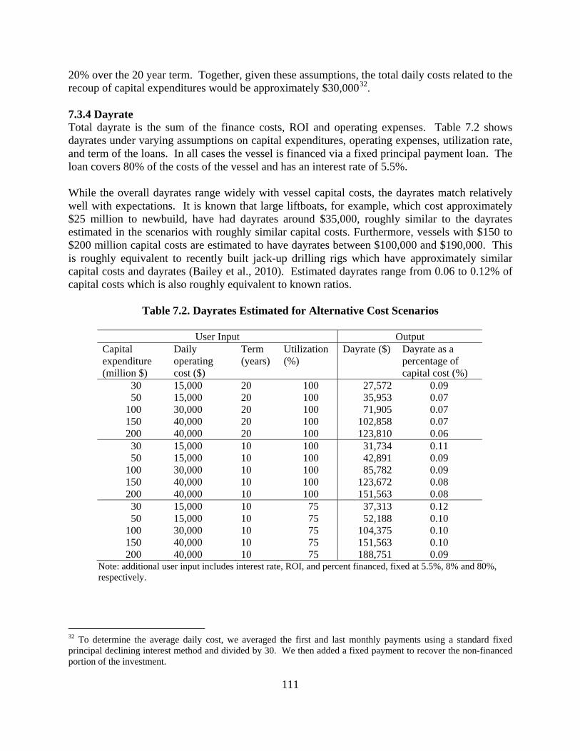
111

20% over the 20 year term. Together, given these assumptions, the total daily costs related to the recoup of capital expenditures would be approximately $30,00032. 7.3.4 Dayrate Total dayrate is the sum of the finance costs, ROI and operating expenses. Table 7.2 shows dayrates under varying assumptions on capital expenditures, operating expenses, utilization rate, and term of the loans. In all cases the vessel is financed via a fixed principal payment loan. The loan covers 80% of the costs of the vessel and has an interest rate of 5.5%. While the overall dayrates range widely with vessel capital costs, the dayrates match relatively well with expectations. It is known that large liftboats, for example, which cost approximately $25 million to newbuild, have had dayrates around $35,000, roughly similar to the dayrates estimated in the scenarios with roughly similar capital costs. Furthermore, vessels with $150 to $200 million capital costs are estimated to have dayrates between $100,000 and $190,000. This is roughly equivalent to recently built jack-up drilling rigs which have approximately similar capital costs and dayrates (Bailey et al., 2010). Estimated dayrates range from 0.06 to 0.12% of capital costs which is also roughly equivalent to known ratios.

Table 7.2. Dayrates Estimated for Alternative Cost Scenarios

User Input Output Capital expenditure (million $)

Daily operating cost ($)

Term (years)

Utilization (%)

Dayrate ($) Dayrate as a percentage of capital cost (%)

30 15,000 20 100 27,572 0.09 50 15,000 20 100 35,953 0.07

100 30,000 20 100 71,905 0.07 150 40,000 20 100 102,858 0.07 200 40,000 20 100 123,810 0.06

30 15,000 10 100 31,734 0.11 50 15,000 10 100 42,891 0.09

100 30,000 10 100 85,782 0.09 150 40,000 10 100 123,672 0.08 200 40,000 10 100 151,563 0.08

30 15,000 10 75 37,313 0.12 50 15,000 10 75 52,188 0.10

100 30,000 10 75 104,375 0.10 150 40,000 10 75 151,563 0.10 200 40,000 10 75 188,751 0.09

Note: additional user input includes interest rate, ROI, and percent financed, fixed at 5.5%, 8% and 80%, respectively.

32 To determine the average daily cost, we averaged the first and last monthly payments using a standard fixed principal declining interest method and divided by 30. We then added a fixed payment to recover the non-financed portion of the investment.

112

In Table 7.3, a regression model of the input-output data is presented33. In the model, the output is DAYRATE ($/day) and the input variables include: CAPEX, the capital costs in million dollars; OPEX, the operating cost in dollars per day; TERM, the term of the loan in years; and UTILIZATION, the utilization rate in percent. Return on investment and interest rates were varied to generate output, but are not included as predictors. The regression is significant (R2 = 0.90) and all parameters have the expected sign: as CAPEX and OPEX increase, DAYRATE increases and as the TERM and UTILIZATION increase, DAYRATE decreases.

Table 7.3. Regression Analysis of the Lease Dayrate Model

DAYRATE = α0 + α1CAPEX + α2OPEX + α3TERM + α4UTILIZATION Parameter α0 α1 α2 α3 α4 Estimate 131,253 763 1 -2,125 -1,333 The fixed cost component of the model (α0) is large and positive. We might expect this component to be zero or nearly zero, suggesting that when all factors are set to zero, the dayrate is zero. Note, however, that when UTILIZATION is set to 100, it is approximately equal to the fixed component, cancelling it out. Therefore, the intercept can be interpreted as being approximately zero with fixed costs accruing as the utilization rate decreases. Table 7.3 is useful for assessing the sensitivity of dayrates to changes in parameters and to quickly specify DAYRATE values for any combination of input value within the bounds of the model. For example, we observe that dayrates are particularly sensitive to changes in utilization rate and loan duration; a one percent increase in utilization rate decreases the dayrate by $1,333, and a one year increase in the term decreases the dayrate by $2,125; a one million dollar increase in capital costs increases the dayrate by just $763. For any given value of input variables, the model regression can be used to estimate dayrates. For example, assume CAPEX is $100 million, OPEX is $40,000 per day, TERM is 15 years and UTILIZATION is 90%. Substituting into the regression equation gives:

DAYRATE = 131,235 + 763*(100) + 1*(40,000) - 2,125*(15) - 1,333*(90)

yielding a dayrate of $95,690. The standard error of the estimate is $23,439 giving a 95% confidence interval of $48,812 to $142,568.

7.4 Dayrates as a Proportion of Newbuild Costs

Dayrates can also be estimated from the capital costs of construction (Cole et al. 1997). There are no available data on the relationship between dayrates and capital costs of offshore wind installation vessels, however, this information can be computed for jackup drilling rigs, liftboats and offshore supply vessels to inform our discussion. Superior Energy Services released information on newbuild and dayrate costs for its large (265 class) liftboats. Superior built two vessels in 2009 for a cost of approximately $25 million and 33 To create the data we systematically varied the input parameters and recorded the output.

113

leased these vessels for approximately 37,500 $/day. This gives a dayrate of approximately 0.15% of newbuild cost (Superior 2010). In its 2009 financial statement, Tidewater provided information on the newbuild cost of domestic and international deepwater platform supply vessels, as well as the annual average dayrates of similar vessels. For domestic vessels, the dayrate was 0.075% of newbuild costs while for international vessels the dayrate was 0.1% of newbuild costs (Tidewater 2009). Using data from Bailey et al. (2010), we estimated the dayrate as a proportion of newbuild cost for jackup rigs. We separated rigs built between 2001 and 2004 into those less than or equal to 300 ft water depth and those greater than 300 ft water depth and derived an average contract build price for each vessel type delivered in a given year. We then divided the average annual dayrate per vessel class by the average newbuild cost34. The average ratio of dayrate to newbuild cost across the eight years in the sample was 0.05% and was similar for both water depth categories. The ratio varied from 0.025% in 2002 to 0.11% in 2006. Bailey et al. (2010) also contains information on the current dayrates and current estimated replacement values of 187 operating jackup rigs. This data differs from the data used previously because it is rig-specific while the dayrate information used above was the average annual dayrate of all rigs in a class. On average, the dayrate is 0.07% of the replacement cost and varied for individual rig contracts from 0.02 to 0.17%. Dayrates across a broad spectrum of vessel classes range from approximately 0.05 to 0.15% of newbuild costs. Since the newbuild costs for turbine installation vessels are known, dayrates can be estimated. Table 7.4 shows these estimates based on a fraction of capital cost.

Table 7.4. Turbine Installation Vessel Dayrates as a Percentage of Capital Costs

Assumed Percentage Capital cost (million $)

0.05% 0.10% 0.15%

30 15,000 30,000 45,000

50 25,000 50,000 75,000

100 50,000 100,000 150,000

150 75,000 150,000 225,000

200 100,000 200,000 300,000

34 However, the contract for a vessel delivered in, for example, 2006 would be related not to the dayrate in 2006, but the dayrate at the time of contract writing some years before 2006. To account for this, we lagged newbuild cost by two years to account for the delay between delivery and the writing of the contract. Therefore, the dayrate in 2004 was divided by the cost of a newbuilt vessel delivered in 2006.

114

7.5 Newbuild Program

Instead of leasing a vessel, a developer may choose to newbuild and operate their own vessel. Two of the most advanced U.S. developers (Bluewater and Deepwater) are pursuing this route. This has not been common in Europe over the past decade, but recently the utility company DONG acquired the turbine installer A2SEA and BARD has used its own vessel to construct the BARD 1 offshore wind farm. The total cost to a developer of using their own newbuilt vessel to install a windfarm is the total financed cost of the vessel plus the total operational costs over the duration of activity. Vessel dayrate can be determined by dividing the total costs by the duration of the activity. However, after building the windfarm, the newbuilt installation vessel has remaining value which must be considered. This value can be estimated in one of two ways: we could assume that after the initial installation the developer leases the vessel over the course of its remaining useful or that the vessel is sold for its depreciated value. Models for both alternatives are derived in Section 7.9. It may be more likely that a developer would seek to lease a vessel after using it for their own installation project, however, in the models developed here, this can generate a negative cost for the initial installation if the expected profit from leasing the vessel over its remaining useful life exceeds the costs of the initial installation. For example, imagine a developer newbuilds a vessel and uses it to install a windfarm at a total cost of $250 million. Over the remaining years of the vessel’s useful life the owner may be able to earn more than $250 million by leasing the vessel to other developers. If this is the case, then the effective cost of the original installation becomes negative suggesting that the profits from leasing a vessel will more than compensate for the costs of using the vessel in installation. Therefore, we assume that the vessel is sold for its depreciated value and that at the time of sale, the proceeds are used to pay off the outstanding debt. This method has the advantage of requiring one less variable as ROI is not needed. Table 7.5 shows estimated dayrates assuming a developer sells their newbuilt installation vessel for its depreciated value at the conclusion of the project. In each scenario in Table 7.5 the interest rate was assumed to be 5.5% with 80% of the total vessel costs financed. Dayrates shown in Table 7.5 are composed largely of operating costs which account for 47 to 69% of dayrates. In Table 7.6, a generalized regression model of the data is developed similar to our previous analysis. The output is again DAYRATE expressed in $/day and the input variables include: CAPEX, the capital costs in million dollars; OPEX, the operating cost in dollars per day; TERM, the term of the loan in years; and DURATION, the length of the project in years. The model describes the data with a near-perfect fit. All of the coefficients are of the expected sign. The model is relatively sensitive to operating costs and insensitive to most other parameters. A one dollar increase in operating expenses increases dayrates by one dollar, but a one million dollar increase in capital costs increases dayrates by only $242. The model does have one non-intuitive result: as the term of the loan increases, the dayrate increases. This suggests that it is cheaper for the owner to obtain a shorter loan because the loan is a fixed principal, declining interest loan that is paid off in full before the end of the loan term. As the term decreases, the monthly

115

principal portion of the payment increases, which decreases the monthly interest payment. The intercept is negative, but it is not statistically different from zero.

116

Table 7.5. Estimated Dayrates for a Developer Using Their Own Newbuilt Vessel, Sold at

the Conclusion of the Project

User Input Output Capital

expenditure (million $)

Daily operating cost ($)

Term (years)

Length of project (years)

Dayrate ($) Dayrate as a percentage of capital

costs (%) 30 15,000 20 3 21,641 0.07 50 15,000 20 3 26,068 0.05

100 30,000 20 3 52,137 0.05 150 40,000 20 3 73,205 0.05 200 40,000 20 3 84,274 0.04 30 15,000 10 3 22,364 0.07 50 15,000 10 3 27,274 0.05

100 30,000 10 3 54,548 0.05 150 40,000 10 3 76,822 0.05 200 40,000 10 3 89,096 0.04 30 15,000 10 6 22,003 0.07 50 15,000 10 6 26,671 0.05

100 30,000 10 6 53,342 0.05 150 40,000 10 6 75,014 0.05 200 40,000 10 6 86,685 0.04

Note: Additional user input includes interest rate, percent financed and life of the vessel, assumed fixed at 5.5%, 80%, and 20 years, respectively.

Table 7.6. Regression Analysis of Costs to a Developer of Newbuilding their own Vessel

DAYRATE = α0 + α1CAPEX + α2OPEX + α3TERM + α4DURATION Parameter α0 α1 α2 α3 α4 Estimate -1,016 242 1 159 -416

7.6 Dayrate Estimation in the U.S.

7.6.1 Limitations The newbuild method demonstrates lower costs than the leasing method. If one of the two methods becomes the dominant means of procuring vessels, the use of the other method in cost estimation is unwarranted and would bias the analysis. Since we do not know which method is more likely, we must consider both. The proportional method yielded the largest range of values, making it potentially less useful than the newbuild and leasing models. However, it is the only empirically derived cost estimate included and requires few assumptions. By contrast, both the leasing and newbuild methods depend on a large number of assumptions. In many cases, the impacts of these assumptions on costs were examined through alternative model parameterizations. However, the models also

117

make implicit assumptions about the methods vessel owners use to determine dayrates; the validity and impact of these assumptions is unknown. In all methods, dayrates or operating expenses from one market (e.g. the GOM liftboat or jackup market) are used to estimate costs in another market (the U.S. offshore wind market). This is necessitated by the nature of the problem but can lead to error. Most notably, error could occur through differences in contract structure. In the offshore wind industry in Europe, dayrates are used as a basis for determining contract costs, but the contract is typically a turnkey contract in which the vessel operator is responsible for engineering costs and risk. By contrast, in dayrate contracts, all logistic and engineering risk is held by the project developer. Future U.S. wind contract structure has not yet been set, but the transfer of risk from the developer to the vessel operator will be associated with cost increases. 7.6.2 Assumptions The three methods developed for estimating dayrates are used to generate a range of values - summing dayrate components; dayrates as a proportion of capital costs; and dayrates for developer-owned vessels - are referred to as “lease”, “proportion” and “build”, respectively. We consider liftboats, jackup barges and SPIVs as candidates for turbine installation vessels in U.S. waters. For each parameter, we assign a minimum and maximum value based on limits derived in Chapter 5 and Sections 6.3. We attempt to be conservative in our parameterization so that all reasonable values are included. This increases the variance in our estimates but makes it more likely that a generic vessel dayrate will fall within the specified range. We assume that liftboats will have a capital cost of approximately $25 to $50 million and operating expenses of 10,000 to 20,000 $/day; that jackup barges will have capital costs $50 to $100 million and operating expenses of 15,000 to 25,000 $/day; and that SPIVs will have capital costs of $150 to $200 million and operating costs between 30,000 and 40,000 $/day. We further assume that all loans are for 80% of the total vessel cost at 4.5 to 6% interest over 10 to 20 years. For the Lease method, the expected return on investment is assumed to range from 7 to 9% and the expected utilization ranges from 75 to 100%. For the Proportion method, we assume that the vessel dayrate is 0.05 to 0.15% of capital costs. For the Build method we assume that the vessel life is 20 years and the project duration is 2 to 5 years. 7.6.3 Results Table 7.7 shows the results for the vessel dayrate. The Proportion method gave the largest range of values while the Build method produced the least variable results. The overall expected dayrate range was in most cases set entirely by the proportion method (i.e. both the largest and smallest values were results of the proportional method). This suggests that if we were less conservative in our interpretation of the dayrate as a proportion of capital costs, the ranges would decrease significantly. The Build method generally produced the lowest results; this might indicate that the build method is the least expensive, however, the build method relies on a secondary market for the

118

vessel; if all developers were to undertake the build method, there would be no secondary market and the build method would be much more expensive. Thus, there may be a frequency dependent relationship between method and cost. The average in Table 7.7 is based on the maximum and minimum values parameterized and does not weight alternative parameterizations by their likelihood. However, given what is known about jackup, liftboat and SPIV vessel dayrates, the averages may be relatively close to the actual dayrates.

Table 7.7. The Range of Vessel Dayrates under Alternative Assumptions and Models

Lease Proportion Build Vessel Min Max Min Max Min Max

Expected value

Dayrate range

Liftboat 19,459 57,307 12,500 75,000 15,582 32,767 35,436 12,500-75,000Jackup Barge 33,919 99,614 25,000 150,000 26,164 50,534 64,205 25,000-150,000SPIV 86,756 189,229 75,000 300,000 63,493 91,068 134,258 60,000-300,000

Note: All dayrates are in $/day

7.7 Mobilization Costs

If installation vessels are moved to another operating region, mobilization costs must be considered. There is an assumption in the literature that mobilization costs for offshore wind are “high” (Kempton et al., 2009; Thresher et al., 2008; Green et al., 2007; Musial et al., 2006; Morgan et al., 2003), however, there has been little quantification of these costs. Typically, mobilization costs are amortized into the dayrate for long term charters. Transport costs could be ignored if they are viewed by the operating company as a permanent relocation of an asset to a new market. In the drilling rig and supply vessel market, long distance movements such as those considered here are often considered investment decisions rather than mobilization to be billed to a single project. The cost of mobilization is a function of the distance, the vessel dayrate, the vessel size and the transport method. Three methods for transport exist: self-propel, semisubmersible heavy-lift transport, or tow. Here, we derive formulas for the costs of mobilization. Costs derived are total costs for a given distance. 7.7.1 Tug Transport Tug transport would likely be used for derrick barges and heavy-lift vessels, and may be used for liftboats, which, although self-propelled, typically travel at or below five knots. The costs of using a tug to pull an installation vessel are given by the time in days times the cost per day plus the costs of insurance. Cost per day is composed of three components: the tug dayrate, the fuel use per day, and the installation vessel dayrate during transport. Formally:

(7-1) where X is the tow distance in nautical miles, Vt is the speed (knots) of the tug, D is the installation vessel displacement (tons), T is the tug dayrate per horsepower ($/day·hp), G is the

119

cost of fuel per gallon ($/gal), I is the installation vessel dayrate ($/day), R is the replacement cost of the installation vessel ($) and Nt is the insurance premium (% of replacement cost) associated with wet tows. Both the tug dayrate and fuel use are a function of the tug horsepower given by 0.011DVt

2 (Zahalka 2008) and the tug is assumed to use one gallon of fuel per horsepower per day35. For application, the displacement will typically range from 4,000 and 20,000 t depending on the vessel specification. Tug dayrates per horsepower vary between 1.35 and 2 (Beegle, Pers. Comm.). Vessel dayrate also depends on vessel specifications and if a lower dayrate for transport is offered. The insurance premium for a wet tow is typically 0.15 to 7.5% of replacement cost (Van Hoorn 1990; Van Horn, Pers. Comm; Offshore Shipping 2000).

7.7.2 Self-Propelled Transport Many turbine installation vessels are self-propelled and are capable of mobilizing without vessel support. In this case, the costs would be the travel time multiplied by dayrate plus fuel costs, or

(7-2)

where Vi is the speed (knots) of the installation vessel and Pi is the installed power (hp). The variables X, I and G are the same as defined in Eq. (7-1). We assume that at cruise speed, 80% of the installed power is utilized (EPA 2000). The installed power typically varies from 4000 to 14,000 hp and the speed ranges from 4 to 12 knots. 7.7.3 Heavy-lift Vessel Transport The cost of heavy transport is a function of the dayrates of the semisubmersible lift vessel and the installation vessel, the distance, fuel use and insurance premium. The total cost is the number of days required for transport, times the daily cost, plus the insurance premium plus the dayrate during loading and unloading:

(7-3) where Vs is the semisubmersible speed (knots), S is the semisubmersible dayrate ($/day), Ps is the power (hp) installed on the semisubmersible heavy lift, and Ns is the insurance premium (%). X, I, G and R are defined in Eq. (7-1). The final term in the equation (2*(S+I)) represents the additional cost required to load and unload a vessel on a semisubmersible vessel; it assumes that one day is needed for unloading and loading. Heavy lift transport via semisubmersible36 may allow for lower insurance premiums than a wet tow. Heavy lift ships would also be capable of transporting larger turbine installation vessels and

35 For dimensional analysis, set 0.011DVt

2 equal to tug hp and since fuel use is 1 gal per hp per day, G can be considered as $/hp·d. 36 Heavy lift transport was used for the transfer of the Titan I and Titan II from the construction shipyard in Louisiana to the UK.

120

derrick barges. Heavy lift transport would likely begin to be favored over wet tows for distances over 1,000 to 2,000 miles. For application, the dayrate for a semisubmersible heavy lift vessel ranges from approximately $50,000 to $100,000 (Van Hoorn Pers. Comm; De Jong 2010). The installed power of semisubmersible lift ships (Ps) ranges from 16,000 to 27,000 hp and the insurance premium for semisubmersible transport is approximately 0.2% (Van Hoorn 1990; Van Hoorn Pers. Comm). 7.7.4 Example Table 7.8 shows the approximate mobilization distances between various locations along the U.S. Gulf and Atlantic coast (Figure 7.6). Each location is in a different planning area and is near an area that could become important for offshore wind energy. Based on these distances, we parameterize the models with five distances: 250, 500, 1000, 1500 and 2000 nautical miles.

Figure 7.6. Hypothetical Mobilization Locations We allow liftboats and large turbine installation vessels to be self-propelled but do not allow barges to be self-propelled. We assume all fuel costs 3 $/gallon; that liftboats and self-propelled vessels travel at 4 and 10 knots, respectively; that vessels travel at 7 knots while under tow; that liftboat displacement ranges from 4,000 to 10,000 t; that barge displacement ranges from 10,000 to 15,000 t; that self-propelled installation vessel displacement varies from 15,000 to 20,000 t; that insurance premiums range from 0.15 to 3% for wet tows37 and are 0.2% for dry transport;

37 Depending on the circumstances of the tow, wet tows may have insurance rates above 3%, however, this produces exceptionally high costs making wet tows extremely costly. If insurance premiums are above 3% there is likely to be no case in which they are favored and we therefore exclude this possibility from the analysis.

121

that installation vessel dayrates are equal to the averages given in Table 7.2; and that the replacement costs of vessels are equivalent to the newbuild costs used above.

Table 7.8. Mobilization Distances* Between Alternative Locations

Galveston, TX

Venice, LA

Jekyl Island, GA

Cape Hatteras, NC

Montauk, NY

Nantucket, MA

Venice, LA 300 Jekyl Island, GA 1,200 1,000 Cape Hatteras, NC 1,500 1,300 400 Montauk, NY 1,900 1,700 800 400 Nantucket, MA 1,950 1,750 850 450 75 Monhegan, ME 2,100 1,900 1,000 600 250 150 Note: *All distances are in nautical miles Table 7.9 shows the results. In cases in which the minimum costs of one mobilization method exceeded the maximum costs of another method, we assumed that the more expensive method would not be used and it was removed from the table. As a result, we do not consider liftboats to be transported by heavy lift for 250, 500, 1,000 or 1,500 nautical mile distances, and we do not consider SPIVs to be transported by wet tow or heavy-lift. We did not allow barges to be self-propelled.

Table 7.9. Ranges of Mobilization Costs* by Method of Mobilization

Tow Self-propelled Heavy lift Vessel type

Distance (nm)

Min Max Min Max Min Max Range Expected value

250 104 1,593 106 177 104-177 129500 171 1,686 213 353 171-353 246

1000 304 1,871 425 707 304-707 4791500 437 2,057 638 1,060 437-1,060 712

Liftboat

2000 570 2,243 851 1,413 1,413 2,310 570-1,413 1,061

250 205 3,156 507 801 205-801 504500 335 3,311 686 1,073 335-1,073 698

1000 595 3,623 1,044 1,618 595-1,618 1,0861500 855 3,934 1,402 2,162 855-2,162 1,473

Jackup Barge

2000 1,115 4,246 1,760 2,707 1115-2,707 1,861

250 151 234 151-234 192500 302 467 302-467 385

1000 604 934 604-934 7691500 907 1,402 907-1,402 1,154

SPIV

2000 1,209 1,869 1,209-1,869 1,539Note: *All costs in $1000

122

The ranges in Table 7.9 were determined as the minimum cost associated with the least expensive method including mobilization, to the maximum costs associated with the next best method. The expected values are the averages of all values included in the range. For example, in the first row of Table 7.9, the range is 104 to 177, but does not include 1,593 because we assume that if this cost is accurate it would never be selected due to the availability of cheaper options. Three values are included in the range (104, 106 and 177) and the expected value is the average of these three values. The costs associated with wet tows varied significantly due to unpredictable insurance costs (Roddick 1995). Insurance rates are highly variable because they are determined on a case-by-case basis and depend on a large variety of mostly unobservable factors. If insurance costs are low, wet tows are generally the cheapest option for liftboats and jackup barges. However, when insurance costs are high, wet tows are never the most economic choice. Overall, mobilization costs range from approximately $100,000 to $3,000,000 depending on transport type, distance and vessel type. Relative to the total installation costs of a project, vessel mobilization is likely to be a small fraction in most cases. Jackups and liftboats had multiple options for mobilization while SPIVs had only a single alternative. This caused the ranges for jackup and liftboat mobilization costs to be greater than those for SPIV costs. In reality the existence of multiple transport options for liftboats and jackups might allow for competition and lower costs.

7.8 Total Vessel Costs

Turbine installation vessel dayrates are estimated based on acquisition strategy and mobilization distance. For example, assume a liftboat is built in Louisiana and is mobilized to Delaware for a project with an expected duration of 1 year. From Table 7.7, the dayrate ranges between 12,500 to 75,000 $/day with an expected value of 35,436 $/day. From Table 7.8 the mobilization distance is approximated based the starting and ending location. In this case, the starting location is near Venice, LA and the end point is between Cape Hatteras, NC and Montauk, NY. We select the 1,500 nautical mile mobilization distance as the most applicable. From Table 7.9, the mobilization costs for a liftboat mobilized 1,500 nautical miles ranges from $437,000 to $1,060,000 with an average value of $712,000. To find the total costs of the project we multiply the dayrate by expected duration of the activity and add the mobilization costs. In this case, the total vessel costs range from $5 to $28 million with an expected value of $13 million. Table 7.10 summarizes the total costs of all vessel types and mobilization distances. To apply the table, select a vessel of interest and a desired mobilization distance. The table provides the total cost for one year of utilization with and without mobilization costs. Demobilization costs are not included, so to find the costs for a two year utilization with demobilization at the end of the project, multiply the costs of one year of utilization with mobilization costs by two. The mobilization costs are typically 2 to 5% of the total costs for a one year project. While mobilization costs are not negligible, in most cases they are small compared to the total vessel costs and nearly negligible compared to the total costs for a large project. In general, previous

123

authors have considered mobilization costs to be significant; based on this analysis, these assumptions seem unfounded. Costs increase as the size of the vessel increases; however, these estimates do not include vessel spreads. Different vessel types will require different support spreads and larger vessels such as SPIVs may require smaller spreads, thereby compensating for their higher costs. Similarly, larger vessels may be able to complete a project in less time than a smaller vessel. Despite the large ranges and generally conservative methods, the overall estimates are modest. The total costs for the use of an SPIV for one year are approximately $50 to $110 million. Assuming an SPIV installs turbine and foundations for a $500 million wind farm over the course of a year, installation costs may range from 10 to 22% of total costs, consistent with previous estimates. While the scenarios described in Table 7.10 are associated with a particular vessel, there is nothing in the dayrate estimates that is vessel specific and estimates could be applied to any vessel with similar capital costs. There are vessel specific factors in the mobilization cost estimates including installed power, vessel speed, and displacement, however, because mobilization costs are a small fraction of total costs, these factors are unlikely to change the total cost estimates significantly.

Table 7.10. Total Vessel Cost* for a One-Year Installation Project

Total cost with mobilization Total cost without mobilization Vessel type Mobilization

distance (nm) Average Min Max Average Min Max

250 13,063 4,667 27,552 12,934 4,563 27,375500 13,180 4,734 27,728 12,934 4,563 27,375

1000 13,413 4,867 28,082 12,934 4,563 27,3751500 13,646 5,000 28,435 12,934 4,563 27,375

Liftboat

2000 14,245 5,133 28,788 12,934 4,563 27,375

250 23,939 9,330 55,551 23,435 9,125 54,750500 24,133 9,460 55,823 23,435 9,125 54,750

1000 24,521 9,720 56,368 23,435 9,125 54,7501500 24,908 9,980 56,912 23,435 9,125 54,750

Jackup Barge

2000 25,296 10,240 57,457 23,435 9,125 54,750

250 49,197 22,051 109,734 49,004 21,900 109,500500 49,389 22,202 109,967 49,004 21,900 109,500

1000 49,774 22,504 110,434 49,004 21,900 109,5001500 50,158 22,807 110,902 49,004 21,900 109,500

SPIV

2000 50,543 23,109 111,369 49,004 21,900 109,500Note: *All costs in $1000

124

7.9 Theoretical Model Development

7.9.1 Leasing Dayrates Dayrates associated with a vessel lease (DL) are composed of three factors: the daily finance costs (Fd), the daily operating costs (O) and the daily ROI (Rd):

(7-4) The daily finance costs are composed of the daily principal and interest payment to the lender plus the daily proportion of the down payment. Over the course of a term loan, the monthly interest payment declines with the declining principal; therefore the finance costs (F) could be determined by either the average interest payment or the specific interest payment. For our purposes, the average interest payment is sufficient and simplifies the equations. In this case, the average monthly principal and interest payment (A) is the first payment plus the last payment divided by two:

(7-5)

where S is the total ship cost, P is the proportion financed, T is the term of the loan and I is the interest rate. In Eq. (7-5), the two terms in square brackets in the numerator are the first and last payments, respectively. Within each bracketed term, the first term (SP/12T) is the monthly principal payment, while the second term is the monthly interest payment. The non-financed portion (N) of the capital costs are then:

(7-6) The daily capital costs (F) are then:

(7-7) where Y equals the life of the vessel in years (alternatively, T could be used instead of Y). To account for unutilized days, the daily finance costs can be divided by the expected utilization rate, Ue. The operating costs, O, are derived from reported annual operating costs divided by utilized days and therefore already account for unutilized periods. The daily ROI (Rd) is the total investment (S) times the annual ROI (RA) divided by 365:

Rd

(7-8)

Rd may also be divided by the expected utilization rate Ue.

125

The total dayrate is thus given by:

(7-9)

7.9.2 Newbuilding Dayrate The dayrate for newbuilding is derived differently from the dayrate for leasing. For newbuilding, the daily cost (DN) to the developer is the total financed cost (FT) divided by the duration of the project (L) in years plus the daily operating expense.

(7-10)

This gives the vessel no value after completion of the project; to give value to the vessel we take the total cost of the project minus the total net income (G) from the vessel after the project, and divide by the duration of the project.

(7-11) In this case, G may be either a lump sum value accrued from the sale of the vessel (GS), or it may be revenue generated from the future lease of the vessel (GL). FT is given by the total vessel cost plus the interest paid where the total interest paid is calculated as the average of the first and last interest payments times the total number of interest payments:

(7-12) which simplifies to:

Assuming the vessel is leased, the total vessel net income following use in the initial wind farm (GL) is a function of the dayrate (not including operating costs), and the remaining life of the vessel:

(7-13) where Y equals the total expected life of the vessel, in years. The dayrate, DL, is given in Eq. (7-9) and represents the net income for a similar vessel. Combining the equations and simplifying gives a total dayrate for a newbuilt vessel to be leased after initial use (DNL) of :

(7-14)

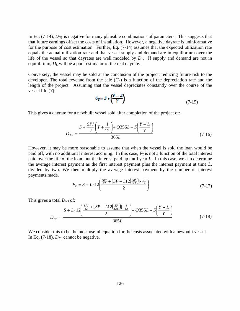
126

In Eq. (7-14), DNL is negative for many plausible combinations of parameters. This suggests that that future earnings offset the costs of installation. However, a negative dayrate is uninformative for the purpose of cost estimation. Further, Eq. (7-14) assumes that the expected utilization rate equals the actual utilization rate and that vessel supply and demand are in equilibrium over the life of the vessel so that dayrates are well modeled by DL. If supply and demand are not in equilibrium, DL will be a poor estimator of the real dayrate. Conversely, the vessel may be sold at the conclusion of the project, reducing future risk to the developer. The total revenue from the sale (GS) is a function of the depreciation rate and the length of the project. Assuming that the vessel depreciates constantly over the course of the vessel life (Y):

(7-15) This gives a dayrate for a newbuilt vessel sold after completion of the project of:

LY

LYSLOT

SPIS

DNS 365

35612

1

2

(7-16)

However, it may be more reasonable to assume that when the vessel is sold the loan would be paid off, with no additional interest accruing. In this case, FT is not a function of the total interest paid over the life of the loan, but the interest paid up until year L. In this case, we can determine the average interest payment as the first interest payment plus the interest payment at time L, divided by two. We then multiply the average interest payment by the number of interest payments made.

2

]12[12 121212

IT

SPSPI

T

LSPLSF (7-17)

This gives a total DNS of:

L

Y

LYSLO

LSPLS

D

IT

SPSPI

NS 365

3562

]12[12 121212

(7-18)

We consider this to be the most useful equation for the costs associated with a newbuilt vessel. In Eq. (7-18), DNS cannot be negative.

127

8. INSTALLATION COST ESTIMATION – REFERENCE CLASS APPROACH

The purpose of this chapter is to review the capital expenditures of European offshore projects and to use this information to infer the installation cost for offshore wind farms in the United States. At present, no offshore wind projects have been developed or are under construction in the U.S., and since there is no direct U.S. experience to draw upon, a comparative (top-down, or reference class) statistical assessment is used in the analysis. We begin by describing cost categories and the basis of the comparative approach. The capital expenditures of European offshore projects are reviewed and analyzed. Capital cost serves as the source data for installation cost estimation and after time and currency adjustment and normalization, a reference class is defined for comparison. Reference class cost estimation has many elements that are advantageous but also some significant drawbacks. A discussion of these advantages and limitations conclude the chapter.

8.1 Cost Categories

8.1.1 Capital and Operating Expenditures The costs associated with developing and operating an offshore wind farm are described in terms of capital and operating expenditures. Capital expenditures (CAPEX) are incurred by purchasing equipment and material to fabricate and install structures. Operating expenditures (OPEX) are incurred through the operation of the physical plant or equipment needed to produce electricity; examples include items such as labor and material, transportation, maintenance and related activity. Normally, capital costs are nonrecurring (i.e., one-time) cost with an expected lifetime greater than one year, whereas operating costs recur for as long as an asset is owned. 8.1.2 Capital Cost Categories For offshore projects, CAPEX is usually classed by:

Development Engineering Equipment Procurement and Delivery Construction

Typically, engineering and development activities contribute 10% or less of the total capital cost of a project. Equipment procurement and delivery is the main cost of offshore development usually ranging between 40-60% of the total project cost (Snyder and Kaiser 2009). Construction involves fabricating, assembly and installation and is the second largest cost category ranging between 20-40% total cost. Installation is a subset of construction activities and typically ranges between 10-30% of the total capital outlay.

8.2 Comparative Method

Significant constraints exist on the manner offshore wind installation cost estimates can be performed. The comparative approach is used as a basis for analogy where project data from a

128

reference class are analyzed to relate to another project or region. If the physical infrastructure in two regions are similar, then the project characteristics may be similar even if other characteristics of development - installation strategies, marine vessels, government regulation, etc. - are different. The implicit assumption of this approach is that the commonalities of offshore wind projects associated with the technology, infrastructure, capital intensity, complexity, and installation requirements outweigh the differences due to environmental, contractual and market conditions. For normalized projects, a reference class approach will yield experience-based statistics. We believe project characteristics and work activities during the early stages of offshore development in the U.S. are likely to be broadly similar to the European experience.

8.3 Source Data

8.3.1 Sample Set Capital expenditures were collected from trade journals, company websites, and academic and government reports. These values were compared using a commercial database (4COffshore) and an industry report (Garrad Hassan 2009). Only wind farms that are operational and generating power, under construction, or for which all capital contracts are finalized are considered. There are a total of 53 offshore wind farms generating power or under construction as of May 2010 (4C Offshore 2010). In addition, there are at least two wind farms for which contracts have been finalized (Lincs and London Array) which gives a total sample of 55 wind farms. 8.3.2 Exclusion Wind farms were excluded from the analysis if there was no reliable information about their costs, if they were built before 2000, or if they were built in Asia. Projects installed before 2000 were excluded because they are primarily of a demonstration character, used small turbines, were placed in benign waters, and are not representative of projects that are currently in development. Projects installed in Asia were excluded because the Asian market is likely to have different costs than the European market. Table 8.1 shows the wind farms included in the sample and the reasons for exclusion. Of the 55 wind farms, 21 were excluded, leaving 34 projects in the total sample. In most cases (13 of 21), wind farms were excluded due to missing data; in four cases, wind farms were excluded due to their age, and in two cases Asian wind farms were excluded. Additionally, the Hywind project was excluded because the reported costs were nearly an order of magnitude higher than the average cost, and Avedore Holmes was excluded as it is not truly offshore. 8.3.3 Reference Class From the 34 wind farms included in the total sample, we created a reference class of wind farms for the purpose of installation cost estimation. In this case, we excluded all wind farms built before 2005 and all wind farms built on non-monopile foundations. The reference class included 18 wind farms. We analyze the capital expenditures of both the total sample and the reference class.

129

8.3.4 Adjustment Costs are adjusted to a single currency (the U.S. Dollar) at a single time (January 1, 2010) to allow for meaningful comparisons. Due to widely varying exchange rates in the sample period, the order in which currency conversion and inflation are performed will impact comparisons.

Table 8.1. Wind Farms Included in the Sample and Reference Class

Name Included in total sample

Reason for exclusion from total sample

Included in reference class

Reason for exclusion from reference class

Arklow Bank Y Y Barrow Y Y Belwind Y Y Burbo Bank Y Y Greater Gabbard Y Y Gunfleet Sands Y Y Horns Rev 2 Y Y Kentish Flats Y Y Lincs Y Y London Array Y Y Lynn/Inner Dowsing

Y Y

OWEZ Y Y Princess Amalia Y Y Rhyl Flats Y Y Robin Rigg Y Y Scroby Sands Y Y Sheringham Shoal Y Y Thanet Y Y Walney Y Y Alpha Ventus Y N FOUNDATION BARD 1 Y N FOUNDATION Beatrice Y N FOUNDATION Blyth Y N AGE Global Tech I Y N FOUNDATION Horns Rev Y N AGE Lillgrund Y N FOUNDATION Middelgrunden Y N FOUNDATION North Hoyle Y N AGE Nysted Y N AGE Rodsand II Y N FOUNDATION Samso Y N AGE Thornton Bank Y N FOUNDATION Utgrunden I Y N AGE Yttre Stengrund Y N AGE Avedore Holme N WD N Baltic I N DATA N

130

Bockstigen N AGE N Breitling N DATA N Cote d'Albatre N DATA N Donghai Bridge N DATA N

Table 8.1. Wind Farms Included in the Sample and Reference Class (continued)

Name Included in total sample

Reason for exclusion from total sample

Included in reference class

Reason for exclusion from reference class

Ems Emden N DATA N Frederikshavn N DATA N Hooksiel N DATA N Hywind N OUTLIER N Kemi Ajos N DATA N Lely N AGE N Roenland N DATA N Setana N GEOG N Sprogo N DATA N Suizhong 36-1 N GEOG N Tricase N DATA N Tuno Knob N AGE N Vindeby N DATA N Vindpark Vanern N DATA N

Notes: DATA = no data, unreliable data, or difficulty finding correlational data; AGE = wind farm built prior to 2000 (total sample) or 2005 (reference class); FOUNDATION = non-monopile foundation; GEOG = excluded for geography; OUTLIER = significant cost outlier; WD = not truly offshore.

There are two options: project costs could be inflated from the year of construction to the present in the reported currency (Euro or Pound), then exchanged to dollars (called inflate first); or project costs could be exchanged to dollars using the exchange rate at the time of construction, then inflated using the U.S. inflation index (called exchange first). See Figure 8.1. We illustrate these options with an example.

131

Figure 8.1. Diagrammatic Depiction of Alternative Methods of Adjusting Costs for a Hypothetical €500 Million Wind Farm Built in 2000 Table 8.2 shows the adjusted costs for a hypothetical €500 million wind farm built between 2000 and 2009. The average Euro and U.S. inflation rates from 2000 to 2009 are 2.57% and 2.16%, respectively. The differences between the two methods are dramatic, especially for wind farms built in the early part of the decade. In most cases, the inflate-first method is less than the exchange-first method. The inflate-first method has less variance because it is a function of two constants (a single exchange rate and a single averaged inflation rate) while the exchange-first method is a function of one variable (the exchange rate at a given time) and one constant (the inflation rate38). We chose to use the inflate-first method since it eliminated one factor that would contribute to variance in cost. Further, while both methods are subject to error due to the fact that capital costs are expended over a period of years rather than at a specific point in time, the effect of this error is likely to be more significant using the exchange first method. The exchange-first method may be more reasonable if the exchange rate at the time of construction impacted contract cost (i.e. if components were sourced from the U.S. and delivered to Europe), but in this case the impact of dollar to euro exchange rate on contract costs is likely minimal.

Table 8.2. Impact of Alternative Methods for Adjusting Costs

Year of completion

Exchange rate

Exchange first

Inflate first

Percent difference

2000 0.92 592.9 866.8 46.2 2001 0.89 559.2 848.4 51.7 2002 0.95 581.9 830.5 42.7 2003 1.13 674.8 813.0 20.5 2004 1.24 722.0 795.8 10.2 2005 1.24 703.9 778.9 10.7 2006 1.25 691.8 762.5 10.2

38 The inflation rate is not truly constant, but was not as variable over the sample period as the exchange rate.

€500

Inflate to 2010 using average currency specific inflation rate

from 2000 to 2009

$460

Convert to $ using 2009 exchange rate

$869

Convert to $ using exchange rate in year of build

€620

Inflate to 2010 using average U.S. inflation rate from 2000 to 2009

$593

Inflate-First Exchange-First

132

2007 1.37 739.2 746.3 1.0 2008 1.47 773.3 730.6 -5.5 2009 1.4 718.0 715.1 -0.4

Project cost data are adjusted using currency inflation rates based on a 10 year average. Exchange rates are based on the average exchange rate in the fourth quarter of 2009. Table 8.3 summarizes the assumptions.

Table 8.3. Inflation and Exchange Rate Cost Normalization Assumptions

Currency Inflation rate (%) Exchange rate to dollars Euro 2.16 1.46 GBP 2.55 1.63 DKK 1.84 0.197 SEK 2.03 0.14 NOK 1.95 0.17

133

Table 8.4. Capital Costs of Offshore Windfarms in the Total Sample

Wind farm Status Capacity (MW)

Cost (Million)

Currency Year online

Source Notes

Alpha Ventus Generating Power 60 250 Euro 2009 Alpha Ventus 2010 Arklow Generating Power 25 45 Euro 2005 Fitzgerald 2005 Bard I Under Construction 400 1400 Euro 2011 European Investment Bank 2010a

Barrow Generating Power 90 123 GBP 2006 BERR 2007a Includes capital grant Beatrice Generating Power 10 35 GBP 2007 Talisman Energy 2007 Includes public sector funding Belwind1 Under Construction 165 614 Euro 2011 European Investment Bank 2010b; Belwind 2010 Blyth Generating Power 4 4 GBP 2000 Pepper 2001 Burbo Bank Generating Power 90 181 Euro 2007 Lemming et al. 2007 Global Tech I Under Construction 400 1200 Euro 2012 European Investment Bank 2010c Greater Gabbard Under Construction 504 1300 GBP 2012 Bradbury 2009 Gunfleet Sands Generating Power 172 3900 DKK 2010 Dong 2007, 2008, 2009a; Stromsta 2010 Horns Rev Generating Power 160 278 Euro 2002 Vatenfall 2010; Gerdes et al., 2006* Includes grid connection Horns Rev II Generating Power 209 3900 DKK 2009 Ministry of Foreign Affairs of Denmark 2010 Kentish Flats Generating Power 90 105 GBP 2005 Vatenfall 2010; BERR 2007b Includes capital grant Lillgrund Generating Power 110 1800 SEK 2007 Vatenfall 2010 Lincs Contracts Signed 270 725 GBP 2012 Lundgren 2009 London Array Contracts Signed 630 2200 Euro 2012 Mastiaux 2010 Lynn/Inner Downsing Generating Power 194 300 GBP 2008 MPI 2010 Middelgrunden Generating Power 40 44.9 Euro 2000 Sorensen et al., 2002 North Hoyle Generating Power 60 82 GBP 2003 Carter 2007* Nysted Generating Power 165 250 Euro 2003 Gerdes et al., 2006* OWEZ Generating Power 108 217.7 Euro 2006 NoordzeeWind 2008* Princess Amalia Generating Power 120 383 Euro 2008 IEA Wind 2009 Rhyl Flats Generating Power 90 190 GBP 2009 May 2009 Robin Rigg Generating Power 180 420 Euro 2008 Mastiaux 2010 Rodsand II Under Construction 207 400 Euro 2011 Mastiaux 2010 Samso Generating Power 23 35 Euro 2003 IEA 2005 Scroby Sands Generating Power 60 73 GBP 2004 Gerdes et al., 2007* O&M removed Sheringham Shoal Under Construction 317 10000 NOK 2011 European Investment Bank 2010d Thanet Under Construction 300 780 GBP 2010 Vatenfall 2010 Thornton Bank Generating Power 30 150 Euro 2009 C-Power 2010 Utgrunden Generating Power 10.5 14 Euro 2000 IEA 2005 Walney Contracts Signed 367 8716 DKK 2011 DONG 2009b; Prysmian 2010Yttre Stengrund Generating Power 10 13 Euro 2001 Barthelmie et al. 2001 Note: Particularly reliable estimate.

134

8.3.5 Normalization All projects were normalized by nameplate capacity and price is expressed in $/MW. Differences in the scope of project costs were taken into account where information was available. For example, the total project cost for Scroby Sands was reported as ₤80.1 million, but 8.5% of the budget covered a five year O&M component; this portion was removed and the final adjusted cost was ₤73.2 million (Gerdes et al. 2006).

8.4 Capital Expenditures

8.4.1 Summary Statistics Table 8.4 shows the nominal capital costs of all offshore wind farms in the sample created by the authors. In Table 8.5, the capital costs from Table 8.4 are depicted along with estimates from a commercial database (4C Offshore) and an industry source (Garrad Hassan; GH). For both our estimates and the 4C Offshore data set, the inflate first method was used. For the GH data, entries were normalized, inflated to 2009 prices, and adjusted to pounds by Garrad Hassan; we then converted to dollars using the 2009 exchange rate. In most cases the values in the three datasets are similar or identical, however, in a few cases the values diverge significantly. Similarity in the values does not imply reliability as the ultimate source of many values is likely to be the same. Differences may be due to the time in which the source estimate was published (i.e. before or after all contracts are finalized), the degree of rounding in the source estimate, the scope of the source39, or methods of adjustment and inflation. We use the average of the three datasets for all subsequent analyses. The average value for all wind farms in the sample was $3.6 million/MW. This estimate is lower than a recent estimate by Ernst and Young (2009) which estimated CAPEX as £3.2 million/MW (approximately $4.8 million/MW at 2009 exchange rates). However, our estimate of $3.6 million/MW is for all wind farms, while the Ernst and Young estimate is for wind farms to be built in the near future. Including only wind farms to be built after 2010, our CAPEX estimate is $4.3 million/MW, similar to the Ernst and Young estimate. The average CAPEX of the reference class is slightly larger than the total sample, while the standard deviation is about half that of the total sample. The reference class is more homogenous than the total sample and is expected to have a smaller variance. The reference class is expected to have more consistent patterns of development and to be reflective of future U.S. development. 8.4.2 Time Trends Historical trends for adjusted, normalized offshore wind CAPEX are shown in Figure 8.2 and Table 8.6. Trends are shown only for the total sample because the reference class is temporally limited. The average cost of offshore wind installation has increased from a low of 2.4 million $/MW from 2000- 2004 to over 4 million $/MW for recent development. Figure 8.2 also shows that price increases have occurred as wind farms have increased in capacity. Capacity increases and learning were assumed to lead to a reduction in offshore wind costs through economies of scale, but factors forcing costs upward have had a greater influence. Reasons for the increase in 39For example, in the Thornton Bank project we used the cost of the first 30 MW phase, while the 4C data reported the estimated cost of the full 300 MW development. Even when normalized for capacity, these estimates differ.

135

project costs have been attributed to several factors, including increasing water depths, increasing commodity costs, reduction and centralization of supply chain competition, and increasing demand for common supply from onshore wind (EWEA 2009).

Table 8.5. Comparison of Normalized Capital Costs by Source (Million $/MW)

Wind farm Authors 4C* GH* Average Alpha Ventus 6.1 6.1 6.6 6.2 Arklow** 2.9 2.9 2.9 Bard I 4.9 4.9 Barrow** 2.4 2.7 2.7 2.6 Beatrice 6.0 6.0 6.0 Belwind** 5.2 2.7 3.9 Blyth 2.0 2.0 2.2 2.1 Burbo Bank** 3.1 3.1 3.1 Global Tech I 4.1 4.5 4.3 Greater Gabbard** 3.9 4.8 6.0 4.9 Gunfleet Sands** 4.4 2.8 4.2 3.8 Horns Rev 2.9 2.9 2.1 2.6 Horns Rev II** 3.7 3.3 4.2 3.7 Kentish Flats** 2.1 2.4 2.3 2.3 Lillgrund 2.4 2.7 2.1 2.4 Lincs** 4.1 4.1 4.1 London Array** 4.8 4.8 4.8 4.8 Lynn/Inner Downsing** 2.6 2.5 3.1 2.7 Middlegrunden 2.0 2.1 1.6 1.9 North Hoyle 2.6 2.5 2.4 2.5 Nysted 2.5 2.5 1.7 2.2 OWEZ** 3.1 2.9 2.7 2.9 Princess Amalia** 4.8 4.4 3.6 4.2 Rhyl Flats** 3.5 3.6 4.4 3.8 Robin Rigg** 3.5 3.6 3.7 3.6 Rodsand II 2.7 2.8 2.7 Samso 2.5 2.2 1.4 2.0 Scroby Sands 2.2 2.3 2.1 2.2 Sheringham Shoal** 5.2 5.2 4.9 5.1 Thanet** 4.1 4.5 5.6 4.8 Thornton Bank 7.3 3.9 7.3 6.2 Utgrunden 2.4 2.2 2.0 2.2 Walney** 4.5 5.1 4.6 4.7 Yttre Stengrund 2.3 2.3 1.7 2.1 Average (SD) - All 3.7 (1.3) 3.4 (1.2) 3.5 (1.7) 3.6 (1.3) Average (SD) – Reference Class** 3.7 (1.0) 3.6 (1.0) 3.9 (1.2) 3.7 (0.9) Note: *4C=4Coffshore (2010), GH = Garrard Hassan (2009);

**= Elements in the reference class. Reference class projects are built after 2005 using monopile foundations and capacity greater than 100MW.

136

Figure 8.2. Offshore Wind Farm Capital Expenditure and Time of Contract for Total Sample. Capacity Size in MW Expressed in Bubble Form.

Table 8.6. Offshore Wind Farm CAPEX by Year of Initial Operation

Year online CAPEX (million $/MW) Number in dataset 2000-2004 2.4 8 2005-2007 3.2 7 2008-2010 4.2 9 2011+ 4.3 9

8.4.3 Economies of Scale The impact of scale economies is difficult to assess since wind farms increased in size over the past decade as prices increased. Table 8.7 shows the cost of wind farms in the total sample by generation category. There is little variation in wind farm costs by capacity, but wind farms over 250 MW are generally more expensive than smaller wind farms, suggesting that economies of scale do not currently govern development. In Table 8.8, the cost of offshore wind farms is presented by capacity and year online. Comparing costs within a time period controls for the effects of time on costs. Comparing across rows, there is no definitive trend of scale economies, however, sample sizes are too small for statistically supported conclusions.

Table 8.7. Average CAPEX by Installed Capacity

Project type Capacity (MW) CAPEX (million $/MW) Number in dataset Demonstration < 20 3.5 3 Pre-Commercial 20 – 100 3.2 11 Small Commercial 100 – 250 3.2 11 Full Commercial 250 – 750 4.6 8

137

Large Commercial > 750 0 Table 8.8. Offshore Wind Farm CAPEX by Capacity and Year Online (Million $/MW)

Capacity (MW) Year online <20 20-100 100-250 250-750 2000-2004 2.2(2) 2.3(4) 2.7(2) 2005-2007 6.0(1) 2.7(4) 2.8(2) 2008-2010 5.2(3) 3.5(5) 4.3(1) 2011+ 3.3(2) 4.6(7) Note: Sample size denoted in parenthesis

8.4.4 Regression Models Regression models of normalized capital costs were constructed based on the linear form:

where Cost is reported in million dollars per MW and variables included installed capacity (MW), water depth (WD, in m), distance to shore (DIS, in km), and a European steel price index, lagged two years so that 2006 steel prices would be used to estimate costs for a wind farm online in 2008 (STEEL). Two indicator variables for gravity (GRAV) and jacket or tripod (JAC) foundations were also included. Indicator variables can be either one (true) or zero (false). For example, if a wind farm uses a gravity foundation, GRAV would be one and JAC would be zero; if a wind farm uses a monopile foundation, GRAV and JAC are zero. The number of turbines and year of installation were removed due to multicolinearity. No interaction terms were evaluated because of the limited size of the sample and constraints on the predictive ability of the variables. Model results are given in Table 8.9. All of the models are statistically significant. Models A-D explain similar proportions of the variance, however, at least one of the coefficients in Models A-C are not significant; therefore, Model D – which contains water depth, steel price and a jacket/tripod indicator variable – is the preferred model. These are the only variables that were consistently significant in the regressions models. The indicator variable for jackets and tripods is a better predictor of cost than the gravity foundation indicator variable. The gravity indicator coefficient was never significant; by contrast the indicator variables for jackets and tripods were usually significant. This implies that for the purpose of capital cost estimation, jackets and tripods should be considered separately. Table 8.9 also shows models for total capital costs. These models explain more of the variance in costs due to the ability of capacity to predict total cost, but are poorly suited to evaluating the impacts of other site-specific variables. Figures 8.3-8.6 show the results of the single variable regressions described in models E-H in Table 8.9. In each case, the models are significant, but do not generally predict a significant portion of the variance. In Figure 8.3, there is a slight positive relationship between capacity and CAPEX; if economies of scale were present, this relationship would be negative. This may be due to the fact that as wind farms increased in size towards the end of the decade, costs increased due to demand from onshore wind. In Figure 8.4, there is a statistically significant relationship

138

between water depth and capital costs; the relationship explains half of the variance in costs. While this is of limited utility as a basis for cost estimation, it does illustrate the importance of water depth on costs. Figure 8.5 shows the influence on distance to shore on CAPEX; the relationship is influenced by two outlying data points associated with two German wind farms (BARD I and Global Tech I). When these outliers are removed, the R2 increases to 0.49. Figure 8.6 shows the influence of steel prices on costs. Steel price index is a reasonable predictor of costs because of its significant role in capital expenditures. Varying the time lag between steel price index and online date did not significantly modify the results.

Figure 8.3. Relationship Between Installed Capacity and Normalized Capital Expenditures

Figure 8.4. Relationship Between Water Depth and Normalized Capital Expenditures

139

140

Table 8.9. Summary of Capital Cost Regression Model

Model α0 α1 α2 α3 α4 α5 α6 R2

A 0.73 0.0011 0.036* -0.0036 0.076 1.59* 0.013* 0.66 B 0.63 0.038* -0.0002 0.023 1.35* 0.014* 0.66 C 0.75 0.0009 0.033* 1.46* 0.013* 0.68 D 0.64 0.037* 1.35* 0.014* 0.67 E 3.03* 0.0031* 0.16 F 2.18* 0.067* 0.51 G 3.03* 0.0241* 0.28

Normalized cost (million $/MW)

H 0.67* 0.020* 0.34 I -110.01* 4.59* 5.66* 0.57 -94.75 27.35 -0.70 0.97 J -222.11* 4.55* 6.49* 0.97

Total cost (million $)

K -121.57* 4.74* 0.96 Note: * Statistically significant (p < 0.05)

141

Figure 8.5. Relationship Between Distance to Shore and Normalized Capital Expenditures

Figure 8.6. Relationship Between European CRU Steel Index and Normalized Capital Expenditures In Figure 8.7, the relationship between capacity and capital expenditures is depicted. Capacity is a very good predictor of capital costs, indicating that capital costs may be reasonably estimated by simply multiplying the average cost per MW by the project capacity.

142

Figure 8.7. Relationship Between Capacity and Capital Expenditures

8.5 Installation Cost Estimation To estimate the installation cost of offshore development, we assume installation cost is a fractional component of capital expenditures. A simple approach to installation cost estimation is required because capital costs are almost never expressed in terms of the categories in which we are interested, namely, procurement, fabrication, assembly and installation. Instead, capital costs are either reported in total, or are broken down into structural components (i.e., turbines, foundation, substation, cabling) to match the way contracts are written. 8.5.1 Model Assumption We assume installation expenditures range between 10 to 30% of total project cost based on a review of available literature. A reasonable expectation on the mean level of installation cost is 20% CAPEX. In Table 8.10, the first three rows estimate the installation cost at three offshore wind farms (Blyth, Scroby Sands, and OWEZ) where reliable data was available. In each case the proportion of total costs ranged from approximately 10 to 30%. The proportion of costs for installation was highest at Blyth, an early small-scale wind farm. The last six rows of Table 8.10 show component installation costs at several different wind farms. Total installation costs as a proportion of capital costs is the sum of turbine, foundation and cable installation. Table 8.10 suggests that each of these activities represents 3 to 6% of capital costs with cable installation being the least expensive and foundation installation being the most expensive. Taken together, these data suggest that approximately 10 to 20% of capital costs are associated with installation. Several generic estimates of offshore wind installation costs also exist (Table 8.11). Estimates range from 10 to 22% of capital costs. Generic estimates are based on model results or industry surveys rather than actual data.

143

144

Table 8.10. Component Cost Estimates of Offshore Wind Farms (No Inflation Adjustment)

Wind farm Scope of work Unadjusted cost (million)

Year Proportion of total cost (%)

Source

Blyth Installation of piles and turbines 1.2 ₤ 2001 31 Pepper 2001 Scroby Sands Offshore installation 16.7 ₤ 2004 23.4 Gerdes et al 2006 OWEZ Installation, including transport 42 € 2008 21 Noordzee Wind 2008 North Hoyle Install 30 monopiles 5 ₤ 2002 6 Maritime Journal 2002 Thanet Install infield and export cables 27 ₤ 2008 3 OilVoice 2008 Robin Rigg Install export cable 7 ₤ 2008 2 4C offshore 2010 Greater Gabbard Install turbines (14 month contract) 62 $ 2009 3 4C offshore 2010 Walney Install turbine (18 month contract) 79 $ 2009 5 4C offshore2010 Sheringham Shoal Install 88 turbines and 2 substation modules 78 € 2009 6 Master Marine 2009

Table 8.11. Estimates of Offshore Installation* Costs Available in the Literature

Source Installation proportion (%) Method Garrad Hassan 2003 22 Generic Model ODE 2007 19 Generic Model DTI 2004 16 Kuhn et al. 1997 7* Generic Model Kooijman et al. 2001 18 Generic Model Schellstsede 2007 9.6 Project Budget Note: * only includes turbine installation

145

8.5.2 Model Results Table 8.12 shows the estimates of installation for existing wind farms in the sample set. The minimum and maximum installation cost is defined to be 10% CAPEX and 30% CAPEX, respectively. The mean estimate for installation is approximately $720,000/MW with a standard deviation of $260,000/MW. Because we are uncertain of both the average capital costs and the proportion of costs attributable to installation, the model gives a large range of potential values. Depending on the user assumptions, three plausible ranges for the installation cost can be adopted based on the average (AVG) and standard deviation (SD) results or the minimum (MIN) and maximum (MAX) of the sample:

I. AVG ± 1*SD II. AVG ± 2*SD

III. MIN – 1*SD, MAX + 1*SD From the model data, these ranges are as follows:

I. $460,000/MW - $980,000/MW II. $200,000/MW - $1,240,000/MW

III. $230,000/MW - $1,470,000/MW For the reference class, the mean estimate increased slightly to $740,000 per MW while the standard deviation declined to $184,000/MW due to the homogeneity of the project data. In this case, the ranges are:

I. $560,000/MW - $924,000/MW II. $372,000/MW - $1,108,000/MW

III. $280,000/MW - $1,386,000/MW Table 8.13 shows the mean installation cost estimate (20%) by year and capacity. Since the mean installation cost estimate is constant, Table 8.13 is derived by multiplying the entries in Table 8.8 by 0.20. The proportion of costs attributable to installation may change with the capacity and year categories shown in Table 8.13 but this not considered in the calculation. 8.5.3 Uncertainty Bounds While the capital costs of future U.S. projects are uncertain, the data suggest that project installation cost between 2005 and 2012 will fall between $372,000 and $1,108,000 per MW, and quite possibly, $560,000 and $924,000 per MW. More of the uncertainty in the estimation is due to variance among projects than differences in our estimates of the proportions of installation cost. If we assume that the mean (20%) value of installation costs is the “real” value, but allow uncertainty in the average capital cost estimate, the range generated by the standard deviation in capital costs alone is $200,000 to $1,240,000 per MW (including all projects). Conversely, if we assume that the mean capital cost is the “real” value, but allow uncertainty around the proportion of capital costs associated with installation (10 to 30%), the range generated by the minimum and maximum installation cost estimates is $360,000 to $1,080,000 per MW. Therefore, given an estimate of capital costs the model can predict the installation costs with increased accuracy.

146

Table 8.12. Estimated Offshore Wind Farm Installation Costs

Installation cost (Million $/MW) Year Wind farm CAPEX (Million $/MW) Min (10%) Mean (20%) Max (30%)

2009 Alpha Ventus 6.25 0.62 1.25 1.87 2005 Arklow 2.89 0.29 0.58 0.87 2011 Bard I 4.90 0.49 0.98 1.47 2006 Barrow 2.61 0.26 0.52 0.78 2007 Beatrice 6.00 0.60 1.20 1.80 2011 Belwind 3.95 0.39 0.79 1.18 2000 Blyth 2.09 0.21 0.42 0.63 2007 Burbo Bank 3.06 0.31 0.61 0.92 2012 Global Tech I 4.28 0.43 0.86 1.28 2012 Greater Gabbard 4.88 0.49 0.98 1.46 2010 Gunfleet Sands 3.80 0.38 0.76 1.14 2002 Horns Rev 2.63 0.26 0.53 0.79 2009 Horns Rev II 3.72 0.37 0.74 1.12 2005 Kentish Flats 2.29 0.23 0.46 0.69 2007 Lillgrund 2.40 0.24 0.48 0.72 2012 Lincs 4.06 0.41 0.81 1.22 2012 London Array 4.80 0.48 0.96 1.44 2008 Lynn/Inner Downsing 2.74 0.27 0.55 0.82 2000 Middlegrunden 1.89 0.19 0.38 0.57 2003 North Hoyle 2.51 0.25 0.50 0.75 2003 Nysted 2.22 0.22 0.44 0.67 2006 OWEZ 2.91 0.29 0.58 0.87 2008 Princess Amalia 4.24 0.42 0.85 1.27 2009 Rhyl Flats 4.01 0.40 0.80 1.20 2008 Robin Rigg 3.60 0.36 0.72 1.08 2011 Rodsand II 2.73 0.27 0.55 0.82 2003 Samso 2.04 0.20 0.41 0.61 2004 Scroby Sands 2.22 0.22 0.44 0.67 2011 Sheringham Shoal 5.07 0.51 1.01 1.52 2010 Thanet 4.75 0.48 0.95 1.43 2009 Thornton Bank 6.16 0.62 1.23 1.85 2000 Utgrunden 2.18 0.22 0.44 0.65 2011 Walney 4.74 0.47 0.95 1.42 2001 Yttre Stengrund 2.10 0.21 0.42 0.63

Average (SD) – All 3.59 (1.28) 0.36 (0.13) 0.72 (0.26) 1.08 (0.39) Average (SD) – Ref. Class* 3.70 (0.92) 0.37(0.092) 0.74 (0.18) 1.11 (0.27)

Note: *Reference class is defined as projects built after 2005 using monopole foundations and minimum capacity 100 MW.

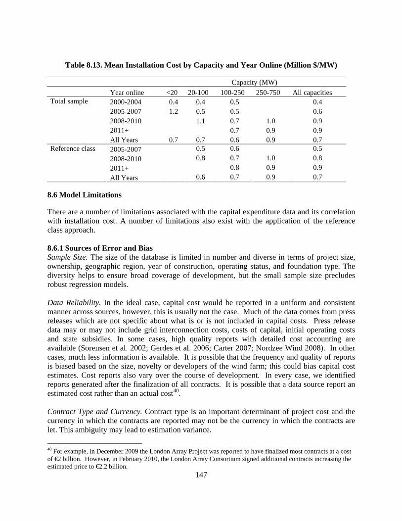
147

Table 8.13. Mean Installation Cost by Capacity and Year Online (Million $/MW)

Capacity (MW) Year online <20 20-100 100-250 250-750 All capacities

2000-2004 0.4 0.4 0.5 0.4 2005-2007 1.2 0.5 0.5 0.6 2008-2010 1.1 0.7 1.0 0.9 2011+ 0.7 0.9 0.9

Total sample

All Years 0.7 0.7 0.6 0.9 0.7 2005-2007 0.5 0.6 0.5 2008-2010 0.8 0.7 1.0 0.8 2011+ 0.8 0.9 0.9

Reference class

All Years 0.6 0.7 0.9 0.7

8.6 Model Limitations

There are a number of limitations associated with the capital expenditure data and its correlation with installation cost. A number of limitations also exist with the application of the reference class approach. 8.6.1 Sources of Error and Bias Sample Size. The size of the database is limited in number and diverse in terms of project size, ownership, geographic region, year of construction, operating status, and foundation type. The diversity helps to ensure broad coverage of development, but the small sample size precludes robust regression models. Data Reliability. In the ideal case, capital cost would be reported in a uniform and consistent manner across sources, however, this is usually not the case. Much of the data comes from press releases which are not specific about what is or is not included in capital costs. Press release data may or may not include grid interconnection costs, costs of capital, initial operating costs and state subsidies. In some cases, high quality reports with detailed cost accounting are available (Sorensen et al. 2002; Gerdes et al. 2006; Carter 2007; Nordzee Wind 2008). In other cases, much less information is available. It is possible that the frequency and quality of reports is biased based on the size, novelty or developers of the wind farm; this could bias capital cost estimates. Cost reports also vary over the course of development. In every case, we identified reports generated after the finalization of all contracts. It is possible that a data source report an estimated cost rather than an actual cost40. Contract Type and Currency. Contract type is an important determinant of project cost and the currency in which the contracts are reported may not be the currency in which the contracts are let. This ambiguity may lead to estimation variance.

40 For example, in December 2009 the London Array Project was reported to have finalized most contracts at a cost of €2 billion. However, in February 2010, the London Array Consortium signed additional contracts increasing the estimated price to €2.2 billion.

148

Exchange Rate Fluctuations. Offshore wind projects have been performed over ten years in several countries and capital costs have been reported in several currencies. Exchange rates fluctuate over time and inflation rates are currency specific. To allow comparisons, all monetary values must be converted to a standardized format; the method of this conversion can cause errors or bias. Normalization. Offshore wind projects are constructed in different environmental conditions and water depths, based upon different technologies and marine vessel spreads, and under different contract requirements. Collectively, these differences create differences in cost. The primary normalization variable is generation capacity; comparisons using a multi-dimensional approach (i.e. multiple regression) are preferred but limited by the size of the data set. Expensing Costs. Project costs may be carried by the developer as overhead. For example, a developer may include support staff or management salaries, facility or equipment costs as overhead. This type of error is likely to produce bias in project comparisons. 8.6.2 Reference Class Constraints There are a number of reasons why the top-down approach is useful for U.S. cost estimation:

Because there is no U.S. activity or project data to draw upon, cost statistics from European

projects are expected to serve as a baseline to U.S. cost.

The infrastructure, technologies, and physical nature of operations and installation requirements in offshore environments are expected to be broadly similar across offshore basins. As long as the similarities of projects dominate the differences (and unfortunately, there is no way to test this assertion until U.S. projects begin construction), the reference class comparison is expected to serve as a useful baseline. If, on the other hand, the differences dominate development, then the reliability of the baseline cost is more limited.

Contract cost is proprietary for competitive reasons, and cost breakdown by stage is either not publicly available or subject to uncertainty because of the manner in which the contract was written. Project CAPEX are available and reasonably certain, and so it is logical to infer installation cost based on assessment of this source data with appropriate assumptions.

Small and diverse sample sets are best characterized by simple statistical measures. Standard deviations allow cost ranges to reflect the level of project uncertainty and scope and the beliefs of the user will dictate which range to select.

The top-down approach is also subject to a number of limitations. The primary obstacles include:

European markets, government support, levels of competition, and marine vessel capability are different than U.S. markets, and if these differences dominate, European cost will be a biased statistic for U.S. projects.

149

European project costs provide guidance on anticipated U.S. cost but do not translate directly. The cost may be subject to escalation or decline factors.

The top down approach relies on historic data which may or may not reflect future realities and is unlikely to be able to account for technical change and learning impacts.

The top down approach assumes that 10 to 30% of capital expenditures are attributable to installation; this assumption is based on limited empirical data. The proportion of costs attributable to installation is variable and future costs may not fall within this range.

150

9. INSTALLATION COST ESTIMATION – ENGINEERING APPROACH

The purpose of this chapter is to develop a model framework to estimate the range of installation costs expected in future U.S. offshore wind development. Our objective is to provide first-order cost estimates based on current technologies and expected market conditions for the period 2011-2016. The model is applicable to shallow water development using monopile foundations and turbine capacities that range between 2.5-5 MW. We begin with an overview of the system and a description of the model input and output. The model framework is outlined and a hypothetical example illustrates the computational procedures. Three U.S. projects in the mid- to late-planning stages (Cape Wind, Bluewater Wind, Coastal Point) are parameterized and installation cost is presented. We conclude with a discussion of the model limitations.

9.1 System Description

9.1.1 User Data Offshore wind farms are characterized by four project descriptors: system generation capacity, turbine capacity, distance to port, and distance to shore. The user is required to provide data on project characteristics, to select a primary installation vessel class and method of installation across each stage of installation, and provide additional information, if known, regarding contract and market conditions expressed through an adjustment factor. 9.1.2 System Data Model-derived data apply empirical relations to compute the inner-array cable length, number of substations required, and the number of export cables. System data specifies vessel configurations, specifications and expected dayrates, unit time statistics per operational stage, and vessel spread requirements. The model derives data from empirical relations based on current project configurations, statistical characteristics computed from the work requirements of installation projects, and vessel dayrates based on hypothetical models. 9.1.3 Model Output Cost calculators based on an engineering approach to estimation are developed across each stage of installation based on project descriptions, user inputs, and system data. In the engineering approach, technical personnel review the requirements of the work activity, and with appropriate assumptions on equipment availability, dayrates, installation methods, time requirements and other factors, estimate the cost of the operation. Each stage of activity is broken down into a number of tasks that must be completed, and once these tasks are defined, a unit cost and time duration is assigned to each. Unit cost and time duration are determined from market and historical data, expert opinion, and other sources. A contingency and weather factor may be incorporated in the estimation. Installation cost is presented according to the following categorization: Foundation, Turbine, Inner-Array Cable, Export Cable, Substation, Scour, and Mobilization.

151

9.2 User Input

Offshore wind farms are characterized by four variables: nameplate capacity (MW), turbine capacity (MW/turbine), distance to port (nautical miles41), and distance to shore (nautical miles). See Figure 9.1. These variables represent the primary configuration variables of offshore wind farms and consolidate the data requirements. The user is required to provide information regarding vessel selection, installation strategy, and contract and market conditions. Default (expected) conditions apply if user data is not specified. Figure 9.1. User-Specified Properties and the Project Parameters They Influence

9.2.1 Project Characteristics Nameplate Capacity The capacity of a wind farm is the main determinant of capital expenditures and is an important parameter in installation cost since the size and number of turbines determines work requirements and vessel selection. Total generation capacity is correlated with the geographic area the turbines require to extract energy from the wind and the cable length to connect individual turbines. Generation capacity and distance to shore determines the need for offshore substations and the number of export cables. Turbine Capacity Turbine capacity for a given system capacity determines the number of turbines and foundations required. Turbine selection, water depth, soil type and wind regime determine the foundation and vessel requirements of installation. Turbine capacity is related to rotor diameter which determines the minimum spacing requirements at the site and inner-array cable length. Distance to Port

41 1 nautical mile = 1.85 km.

152

The distance between the staging area42 and the wind farm determines the time for marine vessels to pick-up material and equipment at port and return to the work site. The number of trips varies with the installation stage, degree of pre-assembly, method of installation, and vessel spread. In turbine installation, it is common practice for the installation vessel to load the turbines at the staging area to avoid offshore transfer operations. For foundation installation, it is common for the installation vessel to remain on site while a vessel spread provides logistical support. For cable installation, distance to port is not expected to be a strong descriptor of operational activity because of the manner in which cable is laid and location of the supply source. Distance to Shore Distance to shore serves as a proxy for the length of export cable required and is a main factor in determining export cable installation cost. Distance to shore is also correlated with water depth which is a factor for vessel selection. Onshore transition type and the presence of biologically sensitive areas will play roles in export cable installation cost but are site-specific and are not considered. Inner-Array Cable Length, Number of Offshore Substations The length of the inner-array cable and number of offshore substations are correlated with the farm generation capacity and distance to shore. If known, they may be provided by the user; otherwise, the model derives expected values for these parameters based on project characteristics. 9.2.2 Vessel Selection The user selects a main vessel for each stage of installation from a list of possible alternatives. When the user selects the vessel type, the model provides transit speed, transport capacity, installation time, dayrate, and spread requirements. The same vessel can be used for foundation and turbine installation and cable laying or separate vessels can be used across each stage. The user can also create a vessel by specifying their own parameters. 9.2.3 Installation Strategy Foundation For foundation installation, two strategies are considered referred to as “self-transport” and “barge”. In self-transport, an installation vessel will pick-up monopiles and transition pieces at the staging area, return to site, and begin operations. In barge installation, a barge will transport the monopiles and transition pieces and the installation vessel stationed at site will perform the required activities; e.g. drive the piles, attach the transition piece, level and grout. We do not allow for monopiles to be wet-towed (floated) to site. Further, we assume that the installation vessel will drive the pile and install the transition piece in sequence. Turbine For turbine installation, all the turbine components - the tower section, nacelle, hub, and blades - will be transported on an installation vessel and assembled at site. The capacity of the vessel to

42 It is possible that more than one staging area will be utilized in fabrication, assembly, and load out, but we do not consider this case. If more than one shore base is utilized, the primary shore base should be selected.

153

transport turbines has a default value by vessel type, but may be modified by the user to account for onshore assembly and reductions in capacity. Cable The methods of installation and vessels that can perform inner-array and export cable installation activities vary widely. For inner-array cable, the most common installation methods involve the use of an ROV operated by either the main installation vessel or a specialized cable-laying vessel. We model only the latter option and assume inner-array cables are installed by a special-purpose vessel. For export cable, installation is carried out in a single continuous operation and transport to and from port is not required43. 9.2.4 Adjustment Factor A user-defined adjustment factor is utilized to discount/escalate cost or activity duration to account for the nature of the activity at the time of operation. The adjustment factor is subjective and depends upon a number of factors that are difficult to predict, including scale economies, learning effects, project novelty, contract terms and levels of competition. An adjustment factor of one indicates no adjustment while an adjustment factor of 1.5 indicates a 50% escalation, and an adjustment factor of 0.5 indicates a 50% discount. Model default value for the adjustment factor is unity. All else equal, we would expect small, near-term projects to have an adjustment factor greater than one due to a lack of scale economies, a slow learning curve, and constrained vessel supply. Application of novel techniques for installation would also induce an adjustment factor greater than one. Assuming that offshore wind development proceeds slowly in U.S. regional markets, one might expect large (> 300 MW), second generation projects with contract finalization after 2020 to have adjustment factors less than one.

9.3 System Data

Parameters enter the model in terms of their maximum, minimum and average value. 9.3.1 Vessel Specification The user selects the vessel class from the available options or creates a new option. Each vessel type is specified by its transport capacity (number of foundations and transition pieces, number of turbine components, tons cable), speed (knots44), expected dayrate ($/day) and installation time (day/foundation, day/transition piece, day/turbine, day/cable km) ranges, and expected spread requirements ($/day). 9.3.2 Expected Time For each stage of activity, a unit time is assigned to perform the work. In foundation and turbine installation, the unit time is derived by model computation based on the user selection of vessel type, installation strategy and distance to port, and the system input of load time, inner-array movement time and installation time. Time is expressed as hours per foundation and hours per turbine. In cable laying, unit time is expressed in days per km installed. For substations and scour protection, a fixed unit time is employed.

43 High voltage export cable is expected to be imported from Europe or Asia by the installation vessel. Transport costs are borne by the developer and would normally be included as part of the installation contract. 44 1 knot = 1.15 mph.

154

9.3.3 Expected Dayrate Each vessel type is associated with an expected dayrate so that selection of the vessel determines the installation dayrate. Vessel type and installation strategy determines the spread requirements and the expected spread dayrate.

9.4 Installation Stage Computations

For each stage of installation, the model computes the expected activity cost as the time required multiplied by the daily cost. Daily cost is the sum of the installation vessel dayrate and the spread dayrate45. Dayrates and spread sizes are determined by user and system input. 9.4.1 Foundation and Turbine Installation Foundation and turbine cost estimates are governed under a similar conceptual framework and are discussed together using the term “unit” to refer to either a foundation or turbine. For foundations, two models are evaluated. In “self-transport”, the main installation vessel transports components, travelling between the support base and the offshore site; in “barge” installation, a feeder barge system is employed (Figure 9.2). For turbines, only the self-transport model is considered; the barge model is rejected due to the risk associated with offshore lifts46. The self-transport models for turbines and foundations are identical in structure and differ only in parameterization. Self-transport In self-transport, the installation vessels pick-up the components for one or more foundations or turbines, deliver them to the work site, and performs installation. Installation proceeds on a per trip basis. The total time per trip is the sum of the travel time, loading time, installation time, and intra-field movement time. When the vessel capacity is exhausted it returns to port for unit replenishment. The total travel time (TRAVEL, hours [h]) is determined by the average speed of the vessel (S, knots [kn]) and the distance to port (D, nautical miles [nm]):

(9-1)

45 Spread dayrate is the sum of the dayrates of all spread vessels required (e.g. tugs, barges, etc.) 46 This reflects current industry practice. In cases where turbine components are supplied by a feeder vessel, the feeder vessel was an elevating main installation vessel. This installation strategy requires a different model structure and is not considered.

155

Figure 9.2. Illustration of Self-Transport and Barge Models Total per-trip installation time (INSTALL, hours [h]), total loading time (LOAD, hours [h]) and total per-trip intra-field movement time (MOVE, hours [h]) are a function of vessel capacity (VC, units/trip) and installation (I, hours [h]), loading (L, hours [h]) and intra-field movement (M, hours [h]) times per turbine: (9-2) (9-3) . (9-4) The total time per trip (TRIP, hours [h]) is the sum of Eqs. (9-1) – (9-4): (9-5) The total time per trip is multiplied by a weather-adjustment factor (W) to account for the proportion of time vessels are able to operate. W = 1 indicates that there are no weather delay, while W = 0.5 indicates that 50% of the time vessels are unable to operate. The weather-adjusted time per trip (ADJTRIP, hours [h]) is:

(9-6)

156

The weather-adjusted time per trip divided by the vessel capacity yields the weather-adjusted installation time per unit (ADJUNIT, hours [h]):

(9-7)

ADJUNIT is compared to known values to determine reasonableness of the assumptions and allows for comparison with the barge model but is not otherwise used in the model. The number of units (NUMUNIT) is computed by the total farm capacity (FC, megawatts [MW]) divided by the turbine capacity (TC, megawatts [MW]):

(9-8)

The number of trips (NUMTRIP) required is determined from the number of units and the vessel capacity:

(9-9)

The installation time (INTTIME, hours [h]) for the total operation is determined from: (9-10) Since the total cost of the project is determined by the total installation time and the daily cost, the total daily cost (TDC, dollars [$]) is the sum of the vessel dayrate (VDR, dollars [$]) and the spread dayrate (SDR, dollars [$]): (9-11) The spread and vessel dayrates are determined from the system input and the user selection of vessel type and installation method (in this case, self-transport). The total cost (COST, dollars [$]) is the installation time (10) normalized to days multiplied by Eq. (9-11):

(9-12)

Cost may be multiplied by the adjustment factor, if desired, to reflect site- and time-specific variations that are not captured in the model framework (e.g., contract type, competition, technology); other fixed costs (project engineering, mobilization) may be added as well. A summary of the model parameters, abbreviations and units is given in Table 9.1 and an example parameterization and calculation steps are provided in Table 9.2. Barge

157

The computational steps of the barge model are illustrated in Table 9.3. In the barge approach, it is assumed that the installation vessel is always supplied with units, so there is no operational downtime47 associated with vessel spread constraints. Since the main installation vessel does not travel to and from port, travel time (TRAVEL) and loading time (LOAD) are not required and the model changes from calculating times per trip to time per unit. The time per unit (UNIT, hours [h]) is the sum of the time to install a unit (I, hours [h]) and move to another intra-field location (M, hours [h]): (9-13) The weather-adjusted time per unit is Eq. (9-13) divided by W:

(9-14)

The total installation time is the product of the weather-adjusted time per unit and the number of units installed: (9-15) As before, the total cost is determined from the product of the time and the daily cost:

(9-16)

9.4.2 Cable Installation Inner-array cables Inner-array cable installation cost (ARRAYCOST, dollars [$]) is determined by the vessel dayrate (ARRAYDR, dollars [$]) and the time required48 (ARRAYTIME, days [d]): (9-17)

47 This is a realistic assumption as long as the vessel spread is adequate. 48 A more complicated model of installation time involving travel time could be developed but was not considered because the data available for parameterization already included transit times. Therefore, adding transit time to the model would double-count.

158

159

Table 9.1. Definition of Terms Used in Foundation and Turbine Installation Models

Variable name

Variable type Models* Description (unit) Value

D User ST Distance to port (nm) FC User ST, B Farm capacity (MW) TC User ST, B Turbine capacity (MW) VC System ST Vessel capacity (number of units) LOAD System ST Load time per trip (h) M System ST, B Inner array move time per unit (h) S System ST, B Vessel speed (knots) I System ST, B Installation time per unit (h) L System ST Load time per unit (h) W System ST, B Weather adjustment factor (%) VDR System ST, B Main installation vessel dayrate ($/day) SDR System ST, B Total spread dayrate ($/day) TDC Computation ST, B Total daily cost ($) VDR +SDR INSTALL Computation ST Installation time per trip (h) VC*I MOVE Computation ST Inner array move time per trip (h) VC*M TRAVEL Computation ST Travel time per trip (h) 2*(D/S) TRIP Computation ST Total time per trip (h) TRAVEL+ LOAD+ INSTALL+ MOVE ADJTRIP Computation ST Weather adjusted time per trip (h) TRIP/W NUMUNIT Computation ST, B Number of units in the farm FC/TC NUMTRIP Computation ST Number of trips required NUMUNIT/VC INTTIME Computation ST Installation time for the total farm (h) ADJTRIP*NUMTRIP COST Computation ST, B Total cost of installation ($) (INTTIME/24)*TDC UNIT Computation B Total time to install one unit and move to next unit (h) I + M ADJUNIT Computation ST, B Weather adjusted time to install one unit and move (h) UNIT/W, (B) or ADJTRIP/VC, (ST) INTTIME Computation B Installation time for the total farm (h) ADJUNIT*NUMUNIT Note: * ST=Self-transport; B= Barge

160

Table 9.2. Example Parameterization and Calculation Steps of the Self-Transport Model

Parameters Step Computation method Example

Determine travel time per trip

Determine installation time per trip

Determine movement time per trip

Determine loading time per trip

Determine total time per trip

Adjust for weather

Determine number of units required

Determine number of trips required

Determine total time required

Determine total daily cost

L = 3 h I = 96 h M = 8 h VC = 4 W = 75% S = 10 knots D = 100 nm VDR = $100,000 SDR = $20,000 FC = 300 MW TC = 3 MW

Determine total cost

161

Table 9.3. Example Parameterization and Calculation Steps of the Barge Model

Parameters

Step Computation method Example

Determine total time per unit

Adjust for weather

Determine no. of units required

Determine total time required

Determine total daily cost

I = 96 h M = 8 h W = 75% VDR = $100,000 SDR = $20,000 FC = 300 MW TC = 3 MW

Determine total cost

ARRAYTIME is determined from the cable length (ARRAYLENGTH, kilometers [km]) divided by the rate (ARRAYRATE, kilometers per day [km/day]) of installation:

(9-18)

Inner-array cable length can be determined through various empirical relations related to rotor diameter and other variables. The relation adopted here describes cable length in terms of farm capacity (FC): (9-19) Export cables Export cable installation cost (EXPORTCOST, dollars [$]) is a function of the installation time (EXPORTTIME, days, [d]) and vessel dayrate (EXPORTDR, dollars [$]): (9-20)

162

EXPORTTIME is set by the cable length (EXPORTLENGTH, kilometers [km]) and the installation rate (EXPORTRATE, kilometers per day [km/day]):

(9-21)

9.4.3 Substation Installation Substation installation is composed of foundation installation and topside installation. We assume that a jacket foundation will be barged to site and placed with a heavy-lift vessel. Pile driving operations secure the jacket to the seabed and represent the primary time in jacket installation. Driving time depends on the soil type, the depth of burial, the size and thickness of the piles, and the number of piles. For topside installation, a heavy-lift vessel is assumed to work for three days. The total cost is the sum of the foundation and topside installation cost. 9.4.4 Scour Protection Scour protection is installed by a barge/tug travelling between port and each turbine site. The total time per trip is composed of loading rock, travel, and installation (dumping) time. Inner-array movement time is ignored. The total tonnage of scour required (TSR, short tons [t]) is given by the tonnage of scour per unit (SPU, short tons [t]) times the number of units (NUMUNIT): (9-22) The number of trips required (SCOURNUMTRIP) is the total scour requirements described by (9-22) divided by the vessel capacity (SCOURVC, short tons [t]):

(9-23)

9.4.5 Mobilization Models for mobilization costs were previously developed (Chapter 7) but since mobilization distances are unlikely to be known until the late planning stages of a project, the user may not feel confident specifying a value. A default value of 1,000 nm is suggested. In either case, a flat-rate based on the average vessel class-specific mobilization cost is added to the total costs. We assume that after project completion the vessel returns to port and demobilization costs are equal to mobilization costs. Spread vessels will be locally supplied in most situations and are assumed to not require mobilization costs.

9.5 Model Parameterization

The model is parameterized based on theoretical and empirical analyses. 9.5.1 Vessel Data In Table 9.4, the turbine and foundation installation vessel parameters are depicted based on the analysis performed in Chapter 6. When the installation vessel is selected, the vessel speed, capacity and dayrates are input into the model. For speed and capacity, the expected value is the average of the range. Table 9.5 summarizes input on spread requirements and costs (from Chapter 5). In developing these costs, the dayrates of tugs, barges and crewboats are assumed to

163

be $10,000/day, $1,750/day and $3,500/day respectively. Spread vessel dayrates were not given a range because the composite dayrate is the relevant variable that will limit the output variance. Vessel spreads are not expected to differ substantially for foundations and turbines.

Table 9.4. Turbine and Foundation Installation Vessel Parameters

Vessel type Speed (kn)

Foundation capacity

Turbine capacity Dayrate range ($/d)

Expected dayrate($/d)

Liftboat 4-6 0 1-2 12,500-75,000 35,400 JU Barge 4-8 2-4 2-6 25,000-150,000 64,200 SPIV 8-12 4-8 6-8 60,000-300,000 134,300

Table 9.5. Total Spread Dayrate Costs by Vessel Category and Transport System

Number of vessels Total dayrate* ($) Vessel type Transport system Tugs Barges Crewboats Min Max Average SPIV Barge 2-3 2-3 2-4 18,500 30,250 24,375SPIV Self-transport 0 0 1-3 2,500 7,500 5,000Jackup Barge 3-4 2-3 2-4 23,500 35,250 29,375Jackup Self-transport 1-2 0 1-3 7,500 17,500 12,500Liftboat Barge 2-3 2-3 2-4 18,500 30,250 24,375Liftboat Self-transport 0-1 0 1-3 2,500 12,500 7,500

Note: * Dayrates of tugs, barges and crewboats are assumed to be $10,000, $1,750 and $3,500, respectively

Table 9.6. Parameterization Range for Factors Influencing Foundation Installation Time

Model Load time, L (h)

Installation time, I (h)

Movement time, M (h)

Weather uptime, W (%)

Self-transport 2-4 (3)* 36-96 (72) 4-8 (6) 75-95 (90) Barge NA 36-96 (72) NA 75-95 (90) Note: * Expected values depicted in parentheses 9.5.2 Foundations Table 9.6 depicts the mean and range of system inputs for loading time, installation time, intra-field movement time and weather uptime. These parameters (together with vessel capacity, speed and distance to port in the self-transport model) determine the time per unit required for installation. The largest single temporal variable in the foundation parameterization is installation time. Installation time consists of the time to drive a pile plus the time to place the transition piece over the monopile, level and grout in place. Pile driving time is estimated based on industry time tables. The depth piles are driven is site-specific and depends upon water depth, soil type, loading requirements and environmental conditions. Most piles to date have been driven 80 to 150 ft into the seabed. Driving rates for 150 to 200 in (4 to 5 m) diameter and 1.5 to 3 in (4 to 8 cm) wall thickness range from 0.2 to 0.4 h/ft. Total pile driving times may thus range from 16 to 60 hours. Time is also required for transition piece placement and grouting. A total installation time range of 36 to 96 hours is considered reasonable in most cases. Wall thickness,

164

pile diameter and insertion depth are determined in part by turbine capacity, and the model is parameterized with short installation times for smaller turbines and longer installation times for larger capacity turbines (Table 9.7). These installation times are chosen to correspond with pile driving times and sizes and to match the overall time distribution.

Table 9.7. Foundation Installation Time as a Function of Turbine Capacity

Turbine capacity (MW)

Installation time range, I (h)

Installation time expected value, I (h)

2.5 36-48 40 3 36-72 54

3.6 48-72 60 4 72-96 84 5 96 96

All capacities 36-96 72 9.5.3 Turbines The mean and range of system inputs for loading time, installation time, intra-field movement time and weather uptime for turbines are shown in Table 9.8. Installation time and vessel capacity may vary with turbine electrical capacity. Increases in turbine capacity will decrease the number of turbines that may be carried per trip and may increase the number of lifts required. The interaction between turbine size, installation time, and vessel choice is shown in Table 9.9, and were estimated based on the data in Table 9.8. Based on the relationship between vessel size and crane capacity, larger, more expensive vessels are assumed to install turbines in fewer lifts and less time than smaller vessels; we assume that a SPIV can install a turbine in half the time required by a liftboat, with a jackup barge approximately intermediate between the two options.

Table 9.8. Parameterization Range for Factors Influencing Turbine Installation Time

Model Load time, L (h)

Installation time, I (h)

Movement time, M (h)

Weather uptime, W (%)

Self-transport 2-6 (4)* 36-120 (72) 4-8 (6) 75-90 (85) Note: * Expected values in parentheses

Table 9.9. Turbine Installation Time by Capacity and Vessel Type

Turbine capacity (MW)

Vessel type Installation time range, I (h)

Installation time expected value, I (h)

LB 72-96 84 JU 48-72 60

2.5 - 3

SPIV 36-48 42 LB 96-120 108 JU 60-96 72

3 - 4

SPIV 48-60 54 LB NA NA JU 72-120 96

4 - 5

SPIV 60-96 72 All capacities 36-120 72

165

9.5.4 Cables Inner-array Inner-array cables are assumed to be installed by either a dynamically positioned self-propelled vessel or a barge-tug system. A medium sized vessel such as a modified offshore supply vessel or a barge-tug spread is expected to have a dayrate of $25,000 (vessels plus ROV) while a larger vessel is expected to have a dayrate of $75,000. Lacking information on vessel type, the model assumes an expected dayrate of $50,000. Installation rate data derived from offshore projects specifies a lay rate of 0.3 km/day with a range of 0.15 to 0.60 km/day. Export High-voltage export cables are heavy and require a large vessel equipped with a high capacity turntable. These vessels are expected to cost approximately 125,000 $/day with a range of $75,000 to $175,000 per day (Howe 2001). Empirically derived export cable installation rates range from 0.2 to 1.4 km/day with an expected value of 0.7 km/day. For a 125,000 $/day vessel laying at 0.7 km/day, the cost of high-voltage cable installation is $178,571 per km49. For medium-voltage export cable, the installation time does not change, but the dayrate is expected to decline slightly. The number of export cables expected in development is obtained from Table 9.10. Cable length is estimated by distance to shore, however, this proxy can be considered a lower bound because of the potential need to avoid sensitive areas or connect to existing onshore infrastructure. Table 9.10. Number of Export Cables and Substations Required by Distance to Shore and

Generation Capacity

Capacity (MW) Distance (km) <100 100-200 200-300 >300

≤10 2* 1-3* 1 2 11 -20 1 1 1 2 21-30 1 1 1 2

Export Cables

>30 1 1 2 2 Substations ≤10 0 0-1 1 1 11-20 1 1 1 2 21-30 1 1 1 2 >30 1 1 1 2

Note: * indicates medium-voltage cable. Relations derived from existing wind farm configurations 9.5.5 Substation Substation foundations are expected to be barged to site; therefore, installation time is simply the time to place the jacket and drive piling, and to apply grout, if required. In some cases a monopile foundation may be used. Pile driving time is expected to range between 0.02 and 0.05 hours per linear foot, assuming pile diameters between 18 to 48 inches and wall thickness of 1 to

49 This compares reasonably well with other estimates. Recently, De Alegria et al. (2009) estimated installation costs for HVAC cable as 100,000 €/km (approximately 134,000 $/km). Other estimates range from 200,000 to 750,000 $/km (Wright et al., 2002; Green et al., 2007; USACE 2004).

166

2 inches. The total pile driving time for 4 to 6 piles, each driven 100 to 150 ft into the seabed will range between 8 and 45 hours with additional time required to reposition the vessel between piles (assumed to be 8 hours total). Most shallow water jackets will weigh between 500 and 1500 tons and require approximately 20 hours to place. Total foundation installation time is expected to range between 1.5 to 3 days. Substation topsides are assumed to require three days to install. We assume a heavy-lift vessel is required for foundation and topside lifting. Heavy-lift vessels are assumed to have dayrates of $80,000 (range $50,000 to $115,000) for lifts under 1000 t, and $150,000 (range $140,000 to $500,000) for lifts over 1000 t. For a lift of unknown weight, we assume $100,000 per day. Additionally, a spread consisting of three tugs, one barge and one crewboat is required at a cost of 19,200 $/day. The number of substations required can be estimated from Table 9.10 based on the distance to shore and farm capacity. 9.5.6 Scour Protection Scour protection is site-specific. In some cases, scour protection may not be needed, while at other locations the amount of protection will vary with the sediment and current conditions (Carter 2007). When needed, the total mass of scour protection required is assumed to be approximately 1250 tons per turbine with a range of 1000 to 1500 tons (Zaaijer and Van der Temple 2004). We assume that a tug and hopper barge travelling at 4 knots with a 1250 t capacity is leased for $8,000 per day. Dumping time is assumed to take 4 hours and loading time is assumed to take 12 hours per trip. 9.5.7 Mobilization Mobilization costs depend on mobilization distances, vessel type, and vessel dayrates. The user may select any mobilization cost from Table 9.11 or the default value of 1000 nm. If dayrates other than the expected dayrates are used, the corresponding mobilization cost should be selected from Table 9.11.

Table 9.11. Ranges of Mobilization Costs* by Mobilization Distance and Vessel Type

Vessel Class Liftboat Jackup barge SPIV Heavy lift Distance (nm) Exp Range Exp Range Exp Range Exp Range

250 129 104-177 504 205-801 192 151-234 273 269-276 500 246 171-353 698 335-1,073 385 302-467 522 476-549

1,000 479 304-707 1,086 595-1,618 769 604-934 1,018 877-1098 1,500 712 437-1,060 1,473 855-2,162 1,154 907-1,402 1,515 1,278-1,6472,000 1,061 570-1,413 1,861 1115-2,707 1,539 1,209-1,869 2,011 1,679-2,196

Note:*All cost in $1000

9.6 Parameter Verification

9.6.1 Temporal Parameters Empirical data on the unit time to install turbines and foundations at existing European wind farms were presented in Chapter 5; these data include travel, loading and installation times as well as weather delays. This empirical data are presented and compared against the weather-adjusted time per unit (ADJUNIT) output from the model to confirm the parameterization. In Table 9.12 the output of a range of assumptions from Table 9.6 are used to estimate the per

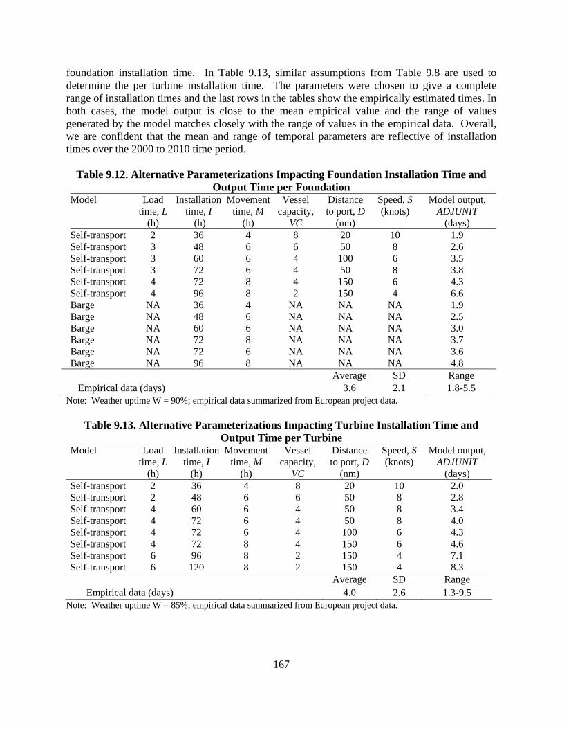
167

foundation installation time. In Table 9.13, similar assumptions from Table 9.8 are used to determine the per turbine installation time. The parameters were chosen to give a complete range of installation times and the last rows in the tables show the empirically estimated times. In both cases, the model output is close to the mean empirical value and the range of values generated by the model matches closely with the range of values in the empirical data. Overall, we are confident that the mean and range of temporal parameters are reflective of installation times over the 2000 to 2010 time period.

Table 9.12. Alternative Parameterizations Impacting Foundation Installation Time and Output Time per Foundation

Model Load time, L

(h)

Installation time, I

(h)

Movement time, M

(h)

Vessel capacity,

VC

Distance to port, D

(nm)

Speed, S (knots)

Model output, ADJUNIT

(days) Self-transport 2 36 4 8 20 10 1.9 Self-transport 3 48 6 6 50 8 2.6 Self-transport 3 60 6 4 100 6 3.5 Self-transport 3 72 6 4 50 8 3.8 Self-transport 4 72 8 4 150 6 4.3 Self-transport 4 96 8 2 150 4 6.6 Barge NA 36 4 NA NA NA 1.9 Barge NA 48 6 NA NA NA 2.5 Barge NA 60 6 NA NA NA 3.0 Barge NA 72 8 NA NA NA 3.7 Barge NA 72 6 NA NA NA 3.6 Barge NA 96 8 NA NA NA 4.8

Average SD Range Empirical data (days) 3.6 2.1 1.8-5.5

Note: Weather uptime W = 90%; empirical data summarized from European project data.

Table 9.13. Alternative Parameterizations Impacting Turbine Installation Time and Output Time per Turbine

Model Load time, L

(h)

Installation time, I

(h)

Movement time, M

(h)

Vessel capacity,

VC

Distance to port, D

(nm)

Speed, S (knots)

Model output, ADJUNIT

(days) Self-transport 2 36 4 8 20 10 2.0 Self-transport 2 48 6 6 50 8 2.8 Self-transport 4 60 6 4 50 8 3.4 Self-transport 4 72 6 4 50 8 4.0 Self-transport 4 72 6 4 100 6 4.3 Self-transport 4 72 8 4 150 6 4.6 Self-transport 6 96 8 2 150 4 7.1 Self-transport 6 120 8 2 150 4 8.3

Average SD Range Empirical data (days) 4.0 2.6 1.3-9.5

Note: Weather uptime W = 85%; empirical data summarized from European project data.

168

9.6.2 Output Costs Installation contracts are proprietary and are generally not publicly available, however, in three recent U.K. projects for turbine installation using SPIVs (Walney, Sheringham Shoal and Greater Gabbard), cost data were made public and is used to serve as a check on parameterization. In cases where the model output deviates from reported data, adjustments to the model parameters to account for known factors yield reasonably accurate cost. This illustrates the unique nature of each project and the need to account for individual project attributes through alternative parameterizations or adjustment factors. Walney Seajacks signed a $70 million turbine installation contract at the Walney windfarm (Blackwell 2009). Walney is composed of 102, 3.6 MW turbines and is 40 nm from port. The effective contract dayrate is $130,000. When these data are input into the model (assuming expected values when not otherwise provided), the average turbine installation time is 3.2 days, the total installation time is approximately 11 months and the estimated cost is $45.9 million (Table 9.14). The difference in cost between the model output and the contract is due to the installation time discrepancy; while both the model and the contract have a similar turbine installation time (1 to 4 per week in the contract and 2.2 per week in the model), the model gives a total work time of 11 months while the contract installation time is 18 months. This discrepancy is due to expected high weather downtime through the winter (DONG 2010). When the weather factor is set at 50%, the estimated cost is $74 million and the total work duration is 17.5 months. While there will be weather delays for U.S. projects, they may not be as severe as those in Europe.

Table 9.14. Parameter Verification from European Windfarms

Contract data Model Output Windfarm Cost

(million $) Duration (months)

Dayrate (1000$)

Cost (million $)

Duration (months)

Cost w/contract dayrate (million $)

Walney 70 18 130 45.9 11 44.5 Sheringham Shoal 101 9 374 37 8.7 104 Greater Gabbard 62 14 147 61.1 13.9 66.7

Sheringham Shoal Master Marine signed a €78 million (approximately $101 million using 2009 exchange rates) contract for turbine installation at the Sheringham Shoal wind farm. Sheringham Shoal will be composed of 88, 3.6 MW turbines and is 20 nm from port. The effective contract dayrate is $374,000. Inserting the default parameters into the model gives an output of $37 million, however, when the model dayrate is changed to reflect the contract dayrate, the model output increases to $104 million (Table 9.14). This suggests that while the model dayrate is too low in this case, the temporal parameters are reasonable. The model dayrate is likely too low because of the extraordinary size and capability of Master Marine’s vessel and high competition for vessel services in the European market; a sister vessel of the one used at Sheringham Shoal received a three year contract for work in the oil industry50 at a dayrate of $300,000. Given the expected pace of development in the U.S. market, we expect the effective dayrate for Master Marine’s 50 For comparison, these dayrates are roughly equivalent to dayrates for semi-submersibles used in the oil and gas industry.

169

vessel to be unrealistic in the U.S. market, unless the project risk is also transferred to the contractor. Greater Gabbard Seajacks signed a $62 million contract to install turbines at the 504 MW Greater Gabbard wind farm. Greater Gabbard is composed of 140, 3.6 MW turbines and is 20 nm from port. The expected installation time is 14 months and the effective dayrate is $147,000. Using model default values yields a cost of $61.1 million and work duration of 13.9 months. Using the dayrate from the contract terms gives an estimated cost of $66.7 million (Table 9.14). In this case, the model output and contract costs match closely.

9.7 Hypothetical 300 MW Windfarm

We illustrate the model using a hypothetical 300 MW wind farm composed of 83, 3.6 MW turbines, 100 nm (185 km) from port and 10 nm (19 km) from shore. Installation vessels are not specified to allow comparisons. Vessel dayrates are fixed at expected values.

Table 9.15. Hypothetical 300 MW Windfarm - Foundation and Turbine Installation Cost

Model Vessel type

Load time, L

(h)

Installation time, I (h)

Movement time, M

(h)

Weather factor, W

(%)

Cost (million $)

Barge JU NA 48 6 90 23.8 Barge JU NA 60 6 90 29.0 Barge JU NA 72 8 75 42.3 Barge SPIV NA 48 6 90 36.3 Barge SPIV NA 60 6 90 44.4 Barge SPIV NA 72 8 75 64.5 Self-transport JU 3 48 6 90 21.0 Self-transport JU 3 60 6 90 25.0 Self-transport JU 4 72 8 75 35.6 Self-transport SPIV 2 48 6 90 31.2 Self-transport SPIV 3 60 6 90 37.7

Foundation

Self-transport SPIV 3 72 8 75 54.5 Self-transport LB 2 96 4 90 23.4 Self-transport JU 2 60 4 90 24.2 Self-transport SPIV 2 48 4 90 30.1 Self-transport LB 4 108 6 85 27.8 Self-transport JU 4 72 6 85 30.8

Turbine

Self-transport SPIV 4 54 6 85 36.6 Self-transport LB 6 120 8 75 34.8 Self-transport JU 6 96 8 75 45.4 Self-transport SPIV 6 60 8 75 46.9

9.7.1 Component Costs Table 9.15 summarizes the cost estimate range for foundation and turbine installation. Jackups and SPIVs are examined using both the barge and self-transport model. In each case, expected values for the vessel speed, capacity, dayrates and spread dayrates are employed. Foundation

170

costs are similar between the barge and self-transport models, but vary by vessel type with jackup barges significantly less expensive than SPIVs. Within a model class and vessel type (and without varying dayrates), the minimum expected cost is approximately 60% of the maximum cost suggesting that variation in activity duration can cause significant uncertainty in cost. A 300 MW wind farm is expected to require approximately 75 km of inner-array cables, and based on its distance from shore (19 km) is expected to require one export cable and substation (from Table 9.10). For mobilization costs, we assume that one heavy-lift vessel, one jackup and one SPIV are mobilized. From Table 9.11, the total mobilization costs are estimated as $2,873,000. The dayrate is constant at $50,000 for inner-array cables and $125,000 for export cables. Given these conditions, Table 9.16 shows cost estimates for cable installation for a variable lay rate. Inner-array cable costs more than export cable, and neither cable installation is as expensive as turbine or foundation installation. The costs of substation installation and scour protection costs are small relative to the total cost and are unlikely to be a major factor.

Table 9.16. Hypothetical 300 MW Windfarm - Cable, Substation, Scour protection Costs

Component Parameterization Lay rate (km/day)

Dayrate ($)

Distance (km)

Cost (million $)

Minimum 0.6 50,000 74.9 6.2 Expected 0.3 50,000 74.9 12.5

Inner array

Maximum 0.15 50,000 74.9 24.0 Minimum 1.4 125,000 37 3.3 Expected 0.7 125,000 37 6.6

Export

Maximum 0.2 125,000 37 23.1 Work duration

(days) Dayrate

($) Spread dayrate

($) Cost

(million $) Substation Minimum 4.2 80,000 19,200 0.42 Expected 5.0 100,000 19,200 0.60 Maximum 5.7 150,000 19,200 0.96 Number of

trips Dayrate

($) Time per trip

(days) Cost

(million $) Minimum 69 8,000 2.75 1.5 Expected 83 8,000 2.75 1.8

Scour protection

Maximum 104 8,000 2.75 2.3 9.7.2 Total Costs Total costs are the sum of the component costs. Table 9.17 shows the expected component costs, the expected total cost, and the costs per stage as a proportion of the total. The total capital costs for a 300 MW wind farm constructed in 2011-2016 are expected to be approximately $1 billion (assuming 3.6 million $/MW). Installation costs are a relatively small proportion of the total costs, approximately 9% in the expected case and up to 14% in the maximum scenario.

Table 9.17. Hypothetical 300 MW Windfarm - Total Costs

Unit Parameterization Foundation1 Turbine2 Inner-array Export Substation Scour Mob Total

171

Minimum 23.8 30.1 6.2 3.3 0.4 1.5 2.9 68.2Expected 29.0 36.6 12.5 6.6 0.6 1.8 2.9 90

Million $

Maximum 42.3 46.9 25.0 23.1 1.0 2.3 2.9 143.5Minimum 34.9 44.1 9.1 4.8 0.6 2.2 4.3 100Expected 32.2 40.7 13.9 7.3 0.7 2.0 3.2 100

Percentage (%)

Maximum 29.5 32.7 17.4 16.1 0.7 1.6 2.0 1009.7.3 Sensitivity Analysis The sensitivity of the self-transport model to changes in farm capacity, distance to port, turbine capacity, installation time, and dayrates is depicted in Figures 3-5. Parameters not otherwise varied are set at their expected values and the costs in the figures represent only the output of the self-transport model for turbine installation. The model scales linearly with farm capacity, dayrate, installation time and distance to port, but nonlinearly with changes in turbine capacity. For every 1 MW increase in farm capacity, the installation cost increases approximately $132,000; for every nautical mile further from port, the cost increases $16,000; for every one-thousand dollar increase in dayrate, the cost increases by $283,000, and for every 1 hour increase in installation time, project costs increase by $569,000. The linearity of the relationship between capacity and cost suggests that economies of scale do not exist relative to farm capacity. The negative relationship shown in Figure 9.4 suggests that there are significant economies associated with increasing turbine size. The sensitivity of the self-transport model to changes in dayrate and installation time is depicted in Figure 9.5. Figure 9.6 depicts changes in vessel class and spread size and the expected per turbine installation time by vessel class. The within-class cost variation shown in Figure 9.6 is due to changing the spread size from the minimum to maximum values (Table 9.5). Given the expected values, liftboats are the least expensive option while SPIVs are more expensive, but as spread costs increase, the difference in vessel costs decrease. Despite the higher cost, SPIVs may be preferred over liftboats due to the expected shorter activity duration. A quicker installation process allows for lower finance costs and lower risks associated with weather delays.

172

Figure 9.3. Sensitivity of the Self-Transport Model to Changes in Capacity and Distance to Port Figure 9.4. Sensitivity of the Self-Transport Model to Changes in Turbine Capacity

Figure 9.5. Sensitivity of the Self-Transport Model to Changes in Dayrate and Installation Time

173

Figure 9.6. Installation Time and Cost Range for High and Low Spread Requirements

9.8 U.S. Proposed Projects

Three U.S. projects in the mid- to late-planning stages are parameterized using publicly available data and cost estimates are derived per stage of installation.

174

9.8.1 Cape Wind - Massachusetts Cape Wind is an offshore project proposed for the south side of Cape Cod and is likely to be one of the first offshore wind developments in the U.S. The BOEMRE has given regulatory approval to project developers, but as of December 2010, construction activities have yet to commence. A detailed Environmental Impact Statement was prepared for the Cape Wind project (MMS 2008) and values from the EIS are utilized. The level of detail provided in the EIS allows for a detailed parameterization. The site selected for Cape Wind is approximately 6 nm from land and will utilize 130, 3.6 MW turbines on monopile foundations for a total nameplate capacity of 468 MW. Foundations are to be installed with a jackup barge using the barge method; turbines are to be installed by a SPIV, similar to European practice. Quonset, Rhode Island is the designated port and is approximately 60 nm to the proposed site. The EIS contains additional information beyond the required user input which can be incorporated into the model. The EIS states the turbine erection is expected to take between 30 and 40 hours per unit (installation time plus inner-array movement time) and that the SPIV is expected to carry 6 to 8 turbines (with transition pieces) per trip. The assumed time to install a monopile is less clear, but the developers state that the monopiles will be installed over an eight month period by two jackup barges. This gives a total time of 480 days and an installation time per monopile (installation time plus inner-array movement time) of approximately 3.7 days (89 hours). Four to 6 spread vessels are expected to support foundation installation, and so the minimum spread cost for a jackup supplied by the barge method is used. For cable installation the EIS estimates that 430 days will be required for the inner-array and 19 days for the export cable. Based on the model parameterization, we would expect installation time to be 537 and 14 days for inner-array and export cables, respectively, but we employ the EIS values. Time to install the substation is estimated as 30 days, however, we suspect this estimate includes a large amount of finishing work (welding on ladders, making electrical connections, etc.) that do not involve the presence of a heavy-lift vessel. Therefore, we employ model estimates for substation installation time. For scour protection, the EIS estimates three days per turbine, and one SPIV, two jackups and one heavy-lift vessel requiring mobilization. The user input and additional input parameters from the EIS are given in Table 9.18. All system parameters not specified in the Table are set at default values. Table 9.18 gives two output costs: one using the EIS input and one using all default parameters. For both outputs, the estimated cost was determined using the expected installation vessel dayrate; the cost range was found by varying the installation vessel dayrate to its minimum and maximum value while leaving all time-related terms constant. Therefore, the maximum and minimum values do not have as great a range as they would if both temporal and dayrate variables were allowed to vary.

Table 9.18. Parameters and Model Output Installation Cost Estimate at Cape Wind

Foundations Turbines Inner-array Export Substation Scour Mob TotalUser input Distance to port

(nm) 60 60

175

Distance to shore (nm)

6

Turbine capacity (MW)

3.6 3.6 3.6

Farm capacity (MW)

468 468 468 468

Vessel type JU SPIV Transport system B ST Spread size Minimum Expected Installation time (h/unit)

84 31

Installation time (d) 430 19 390 Vessel capacity 7

System input

Movement time (h) 5 4 Expected cost 56.0 33.6 21.5 2.4 0.6 3.1 4.0 121.2Maximum cost 102.0 72.9 32.3 3.3 1.0 3.1 7.3 221.9

Output (million $)

Minimum cost 35.0 15.9 10.8 1.4 0.4 3.1 1.5 68.1Expected cost 45.3 56.1 26.9 1.9 0.6 1.4 4.0 136.2Maximum cost 79.4 121.9 40.3 2.7 1.0 1.7 7.3 254.3

Default output (million $) Minimum cost 29.7 26.6 13.4 1.2 0.4 1.1 1.5 73.9 The total cost from the model using the EIS derived input matches relatively closely with the default input and suggests that turbine installation may be more expensive than suggested from the EIS input; this is due to the difference in turbine installation times (60 versus 31 hours in the default and EIS input, respectively). The model output installation cost ranges from $68 to $222 million, with an expected cost of $121 million. These values are slightly lower than the model default cost which ranges from $74 to $254 million with an expected cost of $130 million. Foundations and turbine installation is expected to comprise between 70 to 80% of total installation cost, followed by inner-array cable which accounts for 15 to 19% of the total cost. If Cape Wind is developed at a capital cost of 3.6 million $/MW, the development cost will be approximately $1.68 billion. Expected installation costs range between 7 to 8% of the expected capital costs; the maximum cost range is 13 to 15%. 9.8.2 Bluewater Wind - Delaware Bluewater Wind plans to build a 450 MW wind farm 13 nm off the coast of Delaware. Bluewater Wind signed a Power Purchase Agreement in 2008 and is awaiting regulatory approval and financing. Preliminary planning suggests a development using 3 MW turbines, two substations, and 4 export cables (Bluewater Wind 2010; Musial and Ram 2008). No information on vessel class, supply strategy or port location has been released, however, Bluewater has attempted to secure financing to build its own SPIV (Marine Log 2010) and we assume that an SPIV is the preferred choice for foundation and turbine installation. We assume that the project would use a port facility near Wilmington, DE, approximately 100 nm from the site, and that the barge method is used to supply foundations. All temporal parameters are set to their expected values; dayrates are varied from their minimum to maximum parameterizations. The model output is shown in Table 9.19. The model output installation cost ranges from $84 to $329 million, with an expected cost of $166 million. Foundation and turbine installation is

176

expected to comprise 78 to 85% of total cost; inner-array cable is expected to represent 11 to 15% of total cost. Assuming a capital expenditure of $3.6 million per MW, the installation costs in the expected case are approximately 10% of the total cost.

Table 9.19. Installation Cost Estimate at Bluewater Wind and Coastal Point (Million $)

Bluewater (Delaware) Coastal Point (Texas) Expected Maximum Minimum Expected Maximum Minimum Foundations 66.1 135.2 35.2 7.6 12.7 4.7 Turbines 65.1 142.2 30.3 12.2 23.5 5.7 Inner-array 25 37.6 12.5 4.9 7.4 2.5 Export 4.3 6 2.6 2.6 3.7 1.6 Substation 1.2 2 0.8 0.6 1 0.4 Scour 2.1 2.5 1.6 0 0 0 Mob 1.8 3.6 0.5 0 0 0 Total 165.6 329.1 83.5 27.9 48.3 14.9

9.8.3 Coastal Point - Galveston The Galveston offshore wind project is under development by Coastal Point Energy (formerly WEST) and is planned for Texas State waters approximately 8 nm from shore. The wind farm is designed for 60, 2.5 MW turbines with a total capacity of 150 MW. Tripod foundations are suggested in development plans. Coastal Point has also indicated they will employ a liftboat with a 500 t lift capacity to install foundations and turbines. Public documents indicate that the developers expect foundation installation time to be approximately 1.5 days, consistent with the model estimates for small turbines. We assume that the barge method is used for foundation transport and no mobilization costs are required as liftboat and heavy-lift vessels are common in the Gulf of Mexico. We also assume that scour is not required because of the nature of the foundations. Model output is shown in Table 9.19. The results match relatively well with estimates given by the developers (Schellestede 2008). The developers estimated the costs of foundation and turbine installation as $24.5 million; the expected model output is $19.8 million. The developers expect a total capital cost of $360 million ($2.4 million per MW). At $2.4 million per MW, the expected cost is 8% of the total costs; at $3.6 million/MW, the maximum cost is about 9% of total cost. However, the expected costs assume a vessel dayrate similar to that required for an existing large liftboat. Coastal Point has indicated they may build a larger lift boat which may have costs more similar to the maximum parameterization (Coastal Point Energy 2010).

9.9 Model Limitations

A large number of factors and events impact offshore construction. Selecting a small set of primary variables is only expected to capture a portion of the system complexity. The expectation is that the variables adequately describe the system and proxy the influence of unobservable variables, and in practice, this technique often works reasonably well.

177

There is uncertainty in the duration of work requirements and vessel dayrates and uncertainty in our ability to accurately predict these data from limited and potentially unreliable data. Every factor in the model is subject to these variances, and as these uncertainties propagate through the calculations, cost ranges increase, thus limiting their utility. The expected model results are lower than would be expected from a top-down approach (Chapter 8) unless high dayrate estimates are applied. This may be due to recent capital cost escalation in Europe which has increased total capital expenditures; for a fixed installation cost, increases in capital expenditures will lower the proportion of costs attributable to installation. Therefore, while installation may have been 10 to 30% of total capital costs in the 2002 to 2007 time period, recent increases in non-installation related costs may shrink this proportion. Vessel costs are based on dayrate contracts where the construction and financial risk is held by the developer. In most early European wind farm installations, turnkey contracts transfer the risk to the contractor, leading to higher effective dayrates. In the U.S. no standard contract models have evolved and in this analysis no attempt was made to price this risk; as a result, the expected dayrates may underestimate costs. The model does not include mobilization costs for the export cable laying barge. Cable laying vessels are loaded at the factory, and since there are no factories for marine HVAC cables in the U.S., the barge would be loaded in Europe. Transport costs fall outside of the system boundaries and have not been included in our analysis, and therefore the mobilization of the export cable vessel is not considered. However, these costs could be significant, perhaps in the range of $2 to $10 million. The model was developed and parameterized based on commercial (> 100 MW), monopile projects using 2 to 3 MW turbines installed between 2000 and 2010. Applying the model to U.S. demonstration (< 20 MW) and pre-commercial (20-100 MW) projects, or non-monopile projects will require re-parameterization. Future U.S. developments are likely to use 3.6 to 5 MW turbines and methods, and if vessels and installation times change, or novel techniques or structures are developed outside the realm of established conditions and practice, this will require re-parameterization. At the present time, because no projects have commenced construction in U.S. waters, the ability to calibrate the model is limited, and thus, our confidence in the ability of the model to accurately predict installation cost is similarly limited. We believe our results are the best available give the market and regulatory uncertainties and should be interpreted with a clear understanding of the model caveats for proper application.

178

10. STAGE OF DECOMMISSIONING

Decommissioning requirements for OCS renewable energy facilities require that all facilities be removed and the seafloor cleared of all obstructions at the end of the life of the lease. The purpose of this chapter is to provide an overview of the expected workflows and stages of offshore decommissioning that are likely to arise for offshore wind farms. The offshore wind industry is still in the early years of development, and significant decommissioning activity is not expected for decades. When decommissioning programs are executed, they will have many similarities to the oil and gas industry as well as some significant differences. An understanding of oil and gas decommissioning markets informs our expectations of the general conditions expected to develop in offshore wind. We propose an alternative method for turbine removal that, if feasible, is expected to significantly reduce future decommissioning cost.

10.1 Regulatory Requirements

Energy companies that operate offshore are obligated to remove all structures, clear the site and verify clearance upon lease termination. In federal waters, regulations for decommissioning OCS renewable energy facilities and associated structures are described in 30 CFR, Part 285, Subject I, 285.900-913. All facilities, including pipelines, cable, and other structures and obstructions must be removed when they are no longer used for operations but no later than two years after the termination of the lease, ROW grant, or RUE grant. Requirements for facility removal are described in 285.910: All facilities must be removed to a depth of 15 feet below the mudline. Within 60 days after a facility is removed, the site must be cleared and clearance must be

verified.

The operator may request that certain facilities authorized in the lease or grant be converted to an artificial reef or otherwise toppled in place (285.909). As in the offshore oil and gas industry, all co-lessees and co-grant holders of renewable energy leases are jointly and severally responsible for meeting decommissioning obligations (285.900). In state waters, decommissioning requirements are expected to follow OCS requirements, although at present, state laws are not as well developed. Timing specifications, removal depths, bonding and clearance requirements may vary depending on the state.

10.2 Decommissioning Bonds

Before the BOEMRE will issue a commercial lease or approve an assignment of a commercial lease, the lessee must provide a $100,000 financial assurance which is to be adjusted using the Consumer Price Index – All Urban Consumers (CPI-U) over a 5-year period. For a limited lease, ROW grant or RUE grant, the lessee must provide a $300,000 CPI-U adjusted minimum lease- or grant-specific financial assurance.

179

Before the BOEMRE will approve a Site Assessment Plan (SAP), the lessee must provide a supplemental bond or other financial assurance in an amount determined by the BOEMRE to ensure that all lease obligations are covered, including: the projected amount of rent51 and other expected payments due the Government over the next 12 months; any past due rent and other payments; and the estimated cost of decommissioning met-towers and related facilities as described in the SAP. Before the BOEMRE will approve a Construction and Operations Plan (COP), the lessee must provide a supplemental bond or other financial assurance in an amount determined by the BOEMRE based on the complexity, number, and location of all facilities involved in planned activities and commercial operation. The supplemental financial assurance is in addition to the lease-specific bond and, if applicable, the SAP bond. Before the BOEMRE will allow a lessee to install facilities under the COP, the lessee must provide a decommissioning bond or other financial assurance in an amount determined by the BOEMRE based on the expected decommissioning cost. The decommissioning bond is expected to reflect the actual cost under current technology and prices to remove all the renewable energy facilities. The BOEMRE must also approve the coverage schedule.

10.3 Financial Instruments

To provide evidence of financial responsibility the BOEMRE requires operators to provide insurance, a bond, a lease specific abandonment account, U.S. Treasury notes, or obtain a qualified guarantor. Surety bonds have been the preferred method in the oil and gas sector to satisfy an operator’s obligations and are likely to play a similar role in the offshore wind sector. A surety bond is a guarantee that the surety will perform a duty in the event the lessee is unable to do so. In the case of offshore wind leases, the duty is imposed by law to remove all infrastructure created by development and clear the site to ensure performance of regulatory requirements. Surety bonds are agreements between three parties. These parties are the operator (principal) who is obligated to conduct decommissioning activities in accordance with their lease agreement, the government who acts as an agent of the landowner and is required to ensure successful operations (obligee), and an insurance company (surety) which ensures that money exists to complete decommissioning activities, regardless of the financial capacity of the principal. The surety is only responsible for the insured amount, thus the total costs of decommissioning may not be covered if due to price inflation, low capacity, unexpected circumstances (e.g., hurricane destruction), or a combination of such events, the cost of decommissioning exceed the value of the surety.

10.4 Stages of Offshore Wind Decommissioning

10.4.1 Project Management and Engineering The engineering planning phase of decommissioning consists of a review of all contractual obligations and requirements from lease, operating, production, sales, or regulatory agreements.

51 Rent for OCS limited leases have been set at $3/acre. A fee of $70 for each nautical mile that a ROW crosses is also imposed, along with an additional $5/acre easement for use of the affected area. See Section 3.5.

180

A plan is developed for each phase of the project, and the process of surveying the market for equipment and vessels is initiated. Engineering personnel assess the work requirements and the project management team will report on the options available, including the scope of work that needs to be performed and how best to prepare the bid. Permits are secured from the BOEMRE to remove structures and verify site clearance. All removal options require a disposal plan.

The costs of project management and engineering are difficult to estimate, however, in the early stages of offshore wind decommissioning they may be expected to be high as new techniques and technologies are developed. These techniques may reduce removal costs and could include the use of special purpose decommissioning vessels, methods for toppling turbines, methods for removing copper from cables, methods for floating foundations to the surface, and methods for explosive severance of large diameter piles. 10.4.2 Turbine Removal The first stage in decommissioning begins with the removal of all the wind turbines. In general, turbine removal follows the same process as installation, but reversed. After electrical isolation from the grid and removal of all lubricants, the blades, hub and nacelle will be removed, either singly or together, and the tower section will be unbolted (or cut) and removed. Removal operations occur at the end of the useful life of equipment and are not expected to be as delicate as installation. Since there are several options for turbine installation, several methods exist for removal, and given the expected high cost if vessels similar to installation are required, it is reasonable to assume creative and novel methods will arise. The number of lifts required to remove a turbine depends on the option selected (Figure 10.1). The number of lifts is proportional to time and vessel dayrates will vary with capacity and supply-demand conditions at the time of the operation. The same vessel spread used in installation are likely to be required in a traditional removal because the lift weights have not changed, but the work activity is expected to be somewhat shorter; for a different vessel spread, the installation rates will differ. Workflow The general methodology is as follows: 1. Mobilize vessel and cargo barge to location 2. Cut turbine cables 3. Remove turbine in 1 to 6 lifts 4. Transport all components to an onshore site for reuse, recycling, or disposal.

Reuse, Recycle, Disposal Options The nacelle and hub may be disposed of in a designated landfill or they may be processed to remove steel components to sell as scrap. Blades and cable will be disposed of in a landfill. Towers will be disassembled and sold as scrap steel. Vessel Requirements Based on the size, weight, and height of the turbines, removal operations can be performed with vessels having lift capabilities of 100-200 or more tons. Vessels may be liftboats, jackup barges, or SPIVs. In addition, cargo barges and anchor handling tugs will be required. The cost of cargo

181

barges to transport the turbine components depends on the barge size, mob/demob time and accompanying tugs, and the amount of transported material. Support vessels are assumed to be regionally available and the distance to an onshore facility that can accept the materials will determine the transportation times.

Figure 10.1. Traditional Offshore Turbine Decommissioning Options and an Alternative Alternative Removal Methods Given the high cost of turbine removal, it is reasonable to expect that creative and novel methods will be developed. One method we propose is to fell the turbine in a manner similar to cutting a tree, thereby removing costs associated with disassembly and lifting with heavy-lift vessels (Figure 10.2). All fluids and hazardous material in the nacelle would first be removed, and the turbine tower will be cut and allowed to fall in a controlled manner into the ocean. The turbine would then be lifted onto a barge. The main problems that would need to be overcome under such a scenario are:

Safety; the area must be clear of all personnel, and marine life must be monitored for mammals and sea turtles;

Structural integrity; the turbine component must not hit the water with enough force to break the component.

Flotation; the component must be kept from sinking or easily retrievable after sinking.

182

Weight; a fully assembled turbine may weigh 400 tons and would require a large crane and vessel to lift onto a barge.

Figure 10.2. Proposed Alternative Turbine Removal Method Ensuring flotation of the turbine can be accomplished by making the tower and nacelle watertight. A watertight, submerged turbine tower and nacelle will displace 500 to 1000 tons, and weigh approximately 300 to 500 tons, and will therefore float. However, the nacelle by itself may not be buoyant and might cause the turbine to float vertically. This might require the addition of air bags. The fall of the turbine could be controlled by one or more winches opposing the direction of fall which could be placed on workboats or on nearby turbine foundations. The large weight of the turbine can be overcome by using the buoyancy of the water, cutting the turbine into two or more sections, or using a large crane barge. It is also feasible that some combination of felling and traditional removal methods may be adopted. 10.4.3 Foundation and Transition Piece Removal After the wind turbine is removed, the foundation and transition piece will be removed. It is likely that a vessel different from the turbine removal vessel will perform foundation removals. Cutting Method Foundations are required to be cut 15 ft below the mudline. Mechanical casing cutters, abrasive water jets, diamond wire, or explosives can be used to make the cut at the designated elevation; selection depends upon technical feasibility, environmental conditions, regulatory options, and company preferences. Non-explosive options will likely be preferred because of the size of the monopile and limits on explosive charges. Cutting may be performed internal or external to the monopile. Figure 10.3 depicts the processes required for an external cut; Figure 10.4 depicts the process for an internal cut. For an internal cut, mud is jetted and pumped from the inside of the monopile to the designated below mudline depth; for an external cut, mud will be dredged around the outside of the monopile so that cutting equipment can gain access. The existence of scour protection would add cost and difficulty to an external cut, and for this reason internal cuts are considered more likely. Lifting If the transition piece is grouted onto the monopole, both elements will be lifted together; if the transition piece is attached in another manner, it is conceivable that separate lifts will be performed, but the only economic advantage to performing two lifts is a reduced maximum lift.

183

A reduced maximum lift may translate to a cheaper vessel dayrate, but the incremental benefit is unlikely to account for the additional time required for the operation. A portion of the foundation will remain below the seabed; the transition piece will be removed in its entirety. The weight of the lift is based on the weight of the transition piece, grout, and the cut foundation. The foundation and transition piece will be placed on the removal vessel or cargo barge and returned to shore or to an alternative disposal site.

Figure 10.3. Foundation Removal - External Cut

Figure 10.4. Foundation Removal - Internal Cut Workflow The general methodology for an internal cut is as follows:

1. Gain access to the inside of the pile and set-up jetting and pump equipment 2. Pump mud from inside of monopile

184

3. Cut the monopile 15 feet below the mudline 4. Cut turbine cable at mudline using diver support 5. Remove transition piece and monopile foundation using suitable heavy-lift vessel 6. Transport to onshore location for offloading/disposal or offshore reef site 7. Remove internal equipment and disassemble onshore

Reuse, Recycle, Disposal Options Internal equipment is removed and disassembled and recycled or disposed in an approved landfill. Ancillary material (handrails, boat landing, ladders, etc.) will be disassembled and recycled as scrap steel. Monopiles and transition pieces will be cut into smaller pieces for sale to mini-mills if economic, disposed of in an approved landfill, or transported to an offshore reef site. Vessel Requirements Removal of mud inside the monopile and internal cutting may be performed from a workboat. Excavation by dredge or jetting may be required to overcome the frictional forces during lift. A jackup barge, SPIV or heavy-lift vessel will be required for removal because the lifts are expected to range between 200 and 500 tons. A barge spread for material transport is likely to be used. Alternative Removal Methods Foundations could be removed using novel methods. One possibility would be to float the transition piece to the surface, then tow it to shore, removing the need for a heavy-lift vessel. This would require pumping the mud out of the pile, then cutting the pile, placing an internal water barrier above the cut line, and capping the top of the transition piece. The top of the transition piece could then be connected to a boat or winch and the foundation could be pulled out of the ground and floated. In most cases the pile displacement would be sufficient to float the foundation. Unlike alternative methods of turbine removal, the lower costs of foundation removal may make alternative methods less attractive, and the placement of caps to ensure flotation may not be feasible. 10.4.4 Met Tower and Substation Platform Removal Wind farms will have one or more met towers and possibly one or more substation platforms. These structures may have the same or a different foundation structure relative to the wind turbines. The expected workflow is as follows:

1. Topside structures (meteorological tower, substation transformer) are removed and transported to shore. The met tower may be cut in half or dismantled whole, while the transformer will be lifted whole.

2. For monopile foundations, the monopile will be cut 15 ft below the mudline and removed. For jackets, leg piling will be cut 15 ft below the mudline, and then the piling and jacket will be lifted and removed in a single lift.

3. Transport the structure and superstructure to an onshore or offshore location for offloading/disposal/reefing.

4. Recycle, scrap and landfill.

185

10.4.5 Cable Removal The BOEMRE regulations for power cable and pipeline decommissioning are found at 30 CFR 250.1750-250.1754. OCS pipelines may be left in place when they do not constitute a hazard to navigation, commercial fishing, or unduly interfere with other users. State regulations are similar, but some states require, when feasible, the removal of pipeline segments in the surf zone to a depth of -15 feet MLLW (mean low low water). Regulations on renewable energy power cable decommissioning are not well developed but several options are possible:

Complete removal of all inner-array and export cable through tidelands boundary Leave in place all inner-array and export cable Leave in place a portion of the inner-array and export cable

The decision to remove cable or abandon in place determines the scope of work. In most cases, power cables will not constitute a hazard to navigation, commercial fishing or unduly interfere with other uses, and so are expected to be allowed to remain in place. Power cables may traverse a range of environmental settings, and because burial conditions may change, different solutions are likely to be required. Cable removal will likely be the preferred option when they might interfere with commercial trawling or other activities, they are located in water depths less than -15 feet MLLW or onshore and not deeply buried, or they are located in areas subject to maintenance dredging (Culwell and McCarthy 1998). The removal process involves divers and/or an ROV attaching the cable to a recovery winch. The cable end is retrieved via an engine to drive the cable up onto the recovery vessel. A hydraulic sheer is used to section the cable for storage and transport. Inner-array cable comes in relatively short segments and can be recovered in one piece; if export cable is to be recovered in one piece, a large reel would be needed, or the cable can be cut into pieces as it is recovered. Recovery is not expected to pose technical problems under typical burial conditions due to the high strength of the cable. In-situ abandonment of the inner-array cable would involve cutting the cable at the base of each turbine foundation and bury to a depth of 3 feet. If it is not practical to bury the ends, a concrete cover or mattress may be employed. For export cable a similar procedure would be employed, but at the onshore transition the cable will need to be cut and removed. 10.4.6 Scour Protection It is expected that in many cases scour protection will remain in place in order to minimize disturbance to the seabed and provide a substrate for invertebrates. If scour removal is required, it will be conducted by a mechanical dredge (for rock scour protection) or crane vessel (for concrete mattresses). Scour protection will need to be removed if mandated by regulators or if an external cut is required. 10.4.7 Site Clearance and Verification The last stage in decommissioning is site clearance and verification. Site clearance is the process of removing or otherwise addressing potentially adverse impacts from debris and seafloor disturbances due to offshore wind facilities. Verification is the process of ensuring that site clearance activities are complete.

186

The area encompassed by a commercial wind farm is large, ranging from 0.1 to 0.3 square kilometers per MW capacity, so that a 300 MW wind farm would be expected to cover 30-90 square km. Over a time frame that may exceed 20 years, debris accumulates. Piecemeal salvage is not cost effective and as long as the lost material poses no risk, debris collects over the life of the lease. Once the facilities are removed, however, regulations and lease terms require that the location be left in a state similar to its initial development. In oil and gas operations, regulations specify and contracts are written based on a fixed radius per structure type. In offshore wind farms, there may be up to one hundred or more wind turbines distributed throughout a given area. For clearance purposes, BOEMRE regulations do not specify the area encompassed by the foundation structures. One option is to define the radius of clearance based on the structure function as in oil/gas operations:

Met tower: X ft radius circle centered on the tower52; Monopile foundation with turbine: Y ft radius circle centered on the monopile; Jacket foundations with turbine: Z ft radius circle centered on the platform geometric

center; Monopile/jacket foundations with substation: T ft radius circle centered on the platform

geometric center.

The values of (X,Y,Z,T) would be specified by BOEMRE regulations. Another option is to define the clearance area as the entire wind farm defined by the convex hull created by all the offshore facilities (met tower, turbine, foundations, substation) plus a buffer zone on the boundary of the convex hull. A zone covering the path of the export cables may also be included in defining the area of a wind farm. Current regulations specify that the operator has 60 days from the time an individual structure has been removed to clear the site and verify clearance. An alternative option that may minimize administrative and contractor reporting burden would be to allow clearance to be performed 60 days after the last structure has been removed. There are economies expected to be associated with performing site clearance operations at one time and when other marine vessels are not in the operating theater. In oil and gas operations, the BOEMRE preferred verification technique is to drag a standard trawl net across 100% of the site in two directions. In some cases, alternative site verification techniques such as side scan sonar or documentation of sweep assembly results may be used. Given the large area of windfarms, and the different pattern and magnitude of debris accumulation, it may be reasonable to use or develop alternative methods of site clearance to minimize the negative environmental impacts associated with trawling operations. 10.4.8 Material Disposal There are four methods of disposal for steel and other materials associated with an offshore wind turbine: refurbish and reuse, scrap, dispose of in designated landfills, or place offshore as an artificial reef.

52 For comparison, the radii used in offshore oil regulations are 600 ft for caissons and 1,320 feet for platforms.

187

Opportunities for refurbishing and reusing turbine components, foundations and transition pieces, and power cable are expected to be extremely limited due to the age of the components, the nature of its assembly, and the corrosion arising from operating in a marine environment. Scrapping and recycling are only viable for steel components53, but not all steel components will be economic to be recycled, since the components need to be cut and transported to the point of sale. Cutting steel is expensive, and if the cost to cut and transport steel in saleable units is greater than its resale value, this option will only be pursued if cheaper than the landfill option. Recycle value depends on the weight of the component, cutting cost, scrap steel price, and transportation cost. The transition piece is usually grouted onto the monopile, and so the cost to break the grout adds to the cost to cut the pieces into segments suitable for recycle. In oil and gas decommissioning, scrap often accumulates at onshore yards until scrap steel prices increase to allow a profit to be made on the cutting operations (Kaiser and Pulsipher 2010). It is not clear if the same pattern will hold in other markets where land costs may neither be as abundant nor cheap as in South Louisiana. If a component is not refurbished or scrapped, it will need to be disposed of in a designated landfill. Blades, power cable, some of the nacelle, grout, and marine growth are unlikely to have any resale value and will need to be disposed at a landfill. The cost to dispose depends on the processing cost, transportation cost, and disposal fee. Most of the material from a wind farm is inert and can be disposed of easily; there will be some material that is hazardous, including lubricants and electronics. Some material used in offshore wind farms could be used to make artificial reefs. Singly, monopiles lack the structural complexity required for an artificial reef, however, if a number of monopiles are positioned to achieve structural complexity, then the artificial reef option may be feasible. Other than foundations, no other material would be suitable for reefing54.

53 It is also possible that copper or magnets may be scrapped or recycled, however, the proportional weight of these materials is small. 54 Towers could be used in reef construction but would be easily scrapped.

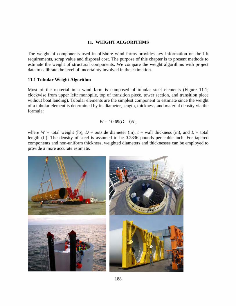
188

11. WEIGHT ALGORITHMS

The weight of components used in offshore wind farms provides key information on the lift requirements, scrap value and disposal cost. The purpose of this chapter is to present methods to estimate the weight of structural components. We compare the weight algorithms with project data to calibrate the level of uncertainty involved in the estimation.

11.1 Tubular Weight Algorithm

Most of the material in a wind farm is composed of tubular steel elements (Figure 11.1; clockwise from upper left: monopile, top of transition piece, tower section, and transition piece without boat landing). Tubular elements are the simplest component to estimate since the weight of a tubular element is determined by its diameter, length, thickness, and material density via the formula:

W = 10.69(D – t)tL,

where W = total weight (lb), D = outside diameter (in), t = wall thickness (in), and L = total length (ft). The density of steel is assumed to be 0.2836 pounds per cubic inch. For tapered components and non-uniform thickness, weighted diameters and thicknesses can be employed to provide a more accurate estimate.

189

Figure 11.1. Scale of Windfarm Tubular Components Source: Weldex DONG Energy 2010b, Liftra,2010, Elsam 2002 In Table 11.1, unit weight in pounds per linear foot is described for a tubular member in terms of outer diameter and thickness. The most common range of weights for monopiles is identified in bold. In Table 11.2, monopile weights were computed via formula and compared to reported weights at selected wind farms. On average, the estimated weights are within 10% of the reported weights. Deviations are due to non-uniform taper and thicknesses; unknown/unreported thickness; and reporting error.

Table 11.1. Tubular Steel Weight (Pounds per Linear Foot) per Diameter and Wall Thickness

Wall Thickness (inches) Nominal Size

(inches) 0.5 1.0 1.5 2.0 2.5 3.0 30 157.7 310.0 457.0 598.6 734.9 865.9 48 253.9 502.4 745.6 983.5 1216.0 1443.2 54 286.0 566.6 841.8 1111.8 1376.3 1635.6 98 521.1 1036.9 1547.4 2052.5 2552.2 3046.7

120 638.7 1272.1 1900.1 2522.8 3140.2 3752.2 150 799.1 1592.8 2381.2 3164.2 3941.9 4714.3 180 959.4 1913.5 2862.2 3805.6 4743.7 5676.4 200 1066.3 2127.3 3182.9 4233.2 5278.2 6317.8

Note: The most common range of weights for monopiles are identified in bold.

Table 11.2. Specifications and Estimated Weights of Monopiles at Selected Wind Farms

Wall thickness Weight Wind farm Length

(m) Outer

diameter (m) Reported

(cm) Assumed

(cm) Reported

(t) Estimated

(t) Kentish Flats 38-44 4.3 4.5 144-184 178-206 Horns Rev 34 4 5 160 164 Horns Rev 2 30-40 3.9 4.0-8.2 150-210 169-226 North Hoyle 50 4 3.0-7.0 5 250 242 OWEZ 45 4.6 4.0-6.0 5 230 250

11.2 Foundations

Foundation lift weight during removal consists of the cut monopile section, the transition piece and the grout. The transition piece is composed of a section of “free” monopile and a section of monopile grouted to the transition piece (referred to as monopile/transition overlap). See Figure 11.2. Monopiles vary in length across wind farms due to varying water depths and geologic conditions.

190

Figure 11.2. Components of a Wind Turbine Foundation 11.2.1 Monopile Monopile weights are frequently reported in development, but in decommissioning it is the weight of monopile removed that is the important factor. Recall that monopiles are cut 15 ft below the mudline as per BOEMRE regulations. Table 11.3 summarizes the monopile removal calculations and assumptions. Table 11.3 assumes a 15 feet below mud line cut, the length of monopile grouted to the transition piece is 1.3 to 1.6 times the pile diameter (Moller 2008; Schaumann et al. 2008), and a wall thickness of 1.5 to 2.5 inches (if exact values are known, they may be utilized).

Table 11.3. Monopile Dimensional Specification Estimates

Specification Unit Assumption Calculation Diameter (D_M) ft 13 to 17 (mean 15) Length of monopile above water (L_MW) ft 3 to 15 (mean 5) Length of total monopile removed (L_TMR) ft WD + 15 + L_MW Monopile/transition overlap factor (OF_MT) 1.3 to 1.6 Length of monopile/transition overlap (L_MT) ft OF_MT * D_M Length of free monopile (L_FM) ft L_TMR – L_MT Wall thickness (WT_M) ft 0.13 to 0.20 Unit weight (UW_M) t/ft 1.25 to 2.25 Weight of total monopile removed (W_TMR) t (WD + L_MW+15)*UW_M Weight of free monopile (W_FM) t UW_M * L_FM Weight of monopile in monopile/transition (W_MMT)

t L_MT * UW_M

To illustrate application of Table 11.3, consider a 15 ft diameter monopile in 30 ft water depth with a wall thickness of 2 inches (Figure 11.3). Assume the pile extends 5 ft above the water line. The total length of the monopile removed is the water depth, plus the 15 feet below mudline, plus the length of monopile above the water line, or 50 ft. The weight of the monopile removed is the length times the unit weight (3,805 lbs/ft, or 1.9 t/ft). Total weight is therefore 50 ft *1.9 t/ft = 95t.

191

The portion of monopile grouted to the transition piece is 1.3 to 1.6 times the pile diameter, or 15 ft*(1.3 to 1.6) = 19.5 to 24 ft. Given the length of monopile/transition overlap and the total length of the monopile, the length of free monopile is the total length minus the length of monopile grouted to the transition piece, or 50 ft – (19.5 to 24 ft) = 26 to 30.5 ft. The weight of free monopile and the weight of monopile grouted to the transition piece is determined by the length times the unit weight: (26 to 30.5 ft)*1.9 t/ft = 49.4 to 58 t. The weight of monopile grouted to the transition piece is (19.5 ft to 24 ft)*1.9 t/ft = 37 to 45.6 t. 11.2.2 Transition Piece If length, diameter and wall thickness of the transition piece is known, weight may be estimated from the tubular steel weight formula. If unknown, values may be estimated as a function of monopile diameter and height above water. Figure 11.3 illustrates the transition piece length estimation method and Table 11.4 gives the calculations, assumptions and nomenclature. Consider a 15 ft diameter monopile that extends 5 feet above the water. Assume the transition piece has a wall thickness of 2 inches (0.17 ft), a height above the water of 50 feet, and an annulus of 0.17 feet (2 inches; 50 mm). Figure 11.3. Transition Piece Height Estimation

Table 11.4. Transition Piece Dimensional Specification Estimation

Specification Unit Assumption Calculation Height above water (H_T) ft 25 to 75 (mean 50) Annulus (A_T) ft 0.17 to 0.4 Length (L_T) ft O_MT + H_T – L_MW Diameter (D_T) ft D_M + (A_T)*2 + (WT_T)*2 Wall thickness (WT_T) ft 0.13 to 0.20 Unit weight (UW_T) t/ft 1.5 to 2.25 Weight (W_T) t UW_T * L_T

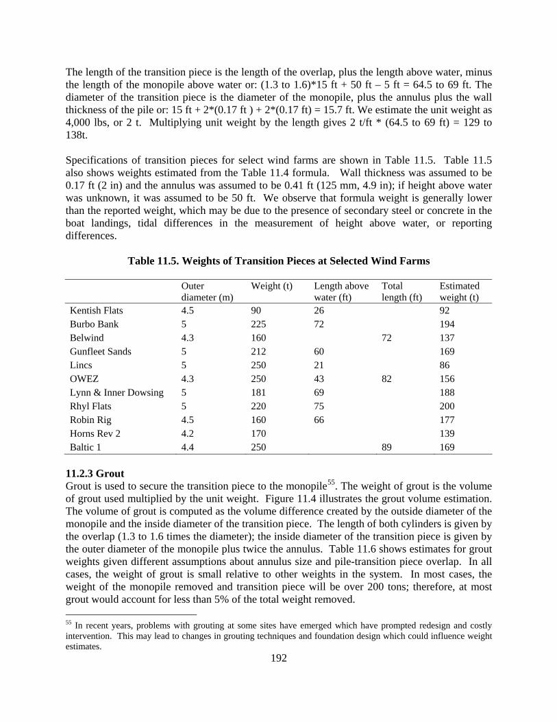
192

The length of the transition piece is the length of the overlap, plus the length above water, minus the length of the monopile above water or: (1.3 to 1.6)*15 ft + 50 ft – 5 ft = 64.5 to 69 ft. The diameter of the transition piece is the diameter of the monopile, plus the annulus plus the wall thickness of the pile or: 15 ft + 2*(0.17 ft ) + 2*(0.17 ft) = 15.7 ft. We estimate the unit weight as 4,000 lbs, or 2 t. Multiplying unit weight by the length gives 2 t/ft * (64.5 to 69 ft) = 129 to 138t. Specifications of transition pieces for select wind farms are shown in Table 11.5. Table 11.5 also shows weights estimated from the Table 11.4 formula. Wall thickness was assumed to be 0.17 ft (2 in) and the annulus was assumed to be 0.41 ft (125 mm, 4.9 in); if height above water was unknown, it was assumed to be 50 ft. We observe that formula weight is generally lower than the reported weight, which may be due to the presence of secondary steel or concrete in the boat landings, tidal differences in the measurement of height above water, or reporting differences.

Table 11.5. Weights of Transition Pieces at Selected Wind Farms

Outer diameter (m)

Weight (t) Length above water (ft)

Total length (ft)

Estimated weight (t)

Kentish Flats 4.5 90 26 92 Burbo Bank 5 225 72 194 Belwind 4.3 160 72 137 Gunfleet Sands 5 212 60 169 Lincs 5 250 21 86 OWEZ 4.3 250 43 82 156 Lynn & Inner Dowsing 5 181 69 188 Rhyl Flats 5 220 75 200 Robin Rig 4.5 160 66 177 Horns Rev 2 4.2 170 139 Baltic 1 4.4 250 89 169

11.2.3 Grout Grout is used to secure the transition piece to the monopile55. The weight of grout is the volume of grout used multiplied by the unit weight. Figure 11.4 illustrates the grout volume estimation. The volume of grout is computed as the volume difference created by the outside diameter of the monopile and the inside diameter of the transition piece. The length of both cylinders is given by the overlap (1.3 to 1.6 times the diameter); the inside diameter of the transition piece is given by the outer diameter of the monopile plus twice the annulus. Table 11.6 shows estimates for grout weights given different assumptions about annulus size and pile-transition piece overlap. In all cases, the weight of grout is small relative to other weights in the system. In most cases, the weight of the monopile removed and transition piece will be over 200 tons; therefore, at most grout would account for less than 5% of the total weight removed. 55 In recent years, problems with grouting at some sites have emerged which have prompted redesign and costly intervention. This may lead to changes in grouting techniques and foundation design which could influence weight estimates.

193

Figure 11.4. Grout Weight Estimation

Table 11.6. Weight of Cement Grout Used in Turbine Foundations

Pile diameter

(m)

Pile overlap as a function of pile

diameter

Annulus width (mm)

Grout volume

(m3)

Weight (t)

4 1.3 50 1.7 2.2 5 1.3 50 2.6 3.5 4 1.6 125 4.9 6.7 5 1.6 125 7.8 10.5

Note: The density of cement is assumed to be 1500 kg/m3 (Zhao et al., 2006).

Table 11.7. Tower Weights by Turbine Type

Turbine Capacity (MW)

Tower (t)

Vestas V80 2 130-200 Vestas V90-3 3 100-150 Siemens 3.6-107 3.6 180-200 Repower 5 M 5 210-225

194

11.3 Tower and Turbine

11.3.1 Tower If turbine tower height, diameter and wall thickness is known or can be reasonably approximated, weight may be calculated via formula. If these variables are not known, they may be estimated from the turbine specifications shown in Table 11.7. The ranges of tower weight for a given turbine are due to differences in hub height. In Table 11.8, the tower length and weight at selected offshore farms are depicted. As the capacity of a turbine increases, weight and load increases, and along with hub height, impacts tower weight. Differences in technology and design account for the variation observed.

Table 11.8. Tower Length and Weight at Selected Offshore Wind Farms

Windfarm Turbine Tower weight (t)

Tower height (m)

Kentish Flats Vestas V90-3 108 62 Horns Rev Vestas V80 160 Gunfleet Sands Siemens 3.6-107 193 60 Alpha Ventus Repower 5 M 210 Burbo Bank Siemens 3.6-107 180 65 Arklow Bank GE 3.6 160 70 Beatrice Repower 5M 225 59

11.3.2 Turbine Turbine rotor and nacelle weights vary based on capacity, blade length, drive type and manufacturer. The most popular European offshore turbines are given in Table 11.9. Much of the weight of the turbine is composed of steel and the turbine can be disassembled and these materials scrapped. However, this may incur significant processing costs because of the manner in which cutting has to be performed. Table 11.10 shows the material composition of turbines by weight. Approximately 70% of the weight of the turbine is composed of steel, some of which may be recycled, depending on processing costs and scrap prices. The steel is primarily in the hub, gearbox and frame, and would be relatively accessible.

Table 11.9. Weight of Turbine Components Turbine Capacity

(MW) Blade length (m)

Rotor (t)

Nacelle (t)

Total (t)

Siemens 2.3-93 2.3 45 60 82 142 Vestas V90-3 3 44 42 70 112 Siemens 3.0-101 3 49 40 73 113 Siemens 3.6-107* 3.6 52 95 125 220 Repower 5 M 5 61.5 120 300 420 Multibrid M5000 5 57 110 199 309 Note: * Cape Wind proposed wind turbines.

195

11.4 Cable

Total cable weight is a function of the weight per meter times the cable length in meters. The weight of cable varies by size and capacity and inner-array cable weight may vary within a wind farm. Export cables generally weigh 50-100 kg/m and inner-array cables weigh 20-40 kg/m.

196

Table 11.10. Proportional Material Usage in Large (4 MW) Turbines

Component Steel (%)

Copper (%)

Other (%)

Proportion of turbine weight* (%)

Blades 2 98 23 Gearbox 96 2 2 30 Generator 93 4 3 8 Frame 85 3 12 20 Hub 100 18 Total 72 1.5 26 100 Note: Turbine weight includes the blades, nacelle and hub. Source: NREL 2008

11.5 Substation

The wind farm substation will be supported on a monopile or jacket foundation. Jackets have more complex geometry and weight depends on framing configuration, the degree of batter, pile requirements, and topsides load. Design philosophy and soil conditions also play a role in determining the amount of steel used in construction. Jacket weights for select wind farms are summarized in Table 11.11 in terms of water depth and topsides load. Topsides for offshore wind substations range in weight from approximately 500 to 2000 tons; the BorWin1 platform is an HVDC platform and is especially heavy. From the data in Table 11.11 we estimated the following functional relationship:

Jacket weight = 12.8 * Water depth0.19 * Topside load0.48

where weight is in metric tons and water depth is in feet.

Table 11.11. Weights of Jackets at Selected Offshore Wind Farms

Wind farm Weight (metric tons)

Water depth (ft)

Topside load (metric tons)

Walney 990 98 1030 Alpha Ventus 750 98 700 Horns Rev 2 800 43 1230 Generic UK, ISC 1200 62 1600 Generic North Sea, ISC 1400 79 1800 Lincs 950 33 2250 Thanet 695 69 1200 BorWin1 1700 130 3200 Greater Gabbard 767 100 2069

197

12. DECOMMISSIONING COST ESTIMATION

Offshore renewable energy facilities are required to be decommissioned and removed and the seafloor cleared of all obstructions at the end of the life of the lease. From the operator’s point of view, decommissioning activities represent a cost to be incurred in the future, while from the government’s perspective, decommissioning represents an uncertain event and financial risk if the operator becomes insolvent or cannot meet its financial obligations under the lease. For this reason, state and federal governments require companies to post a decommissioning bond at the time of construction to ensure that adequate funds exist to remove infrastructure in the future. The level of the bond is usually set at the expected cost to decommission the facilities and may be inflation-adjusted. The purpose of this chapter is to provide first-order decommissioning cost estimates for proposed U.S. offshore wind farms across each stage of activity. Removal and site clearance cost is estimated using empirical and hypothetical relations under current technology and market conditions without inflationary adjustment. Preliminary development plans characterize and define the system and serve as input data for the model. We illustrate the methodology on Cape Wind's proposed project which is furthest along in the development stage. Cost estimates for other proposed U.S. offshore wind farms are also outlined.

12.1 Decommissioning Stages

Decommissioning activities are driven by economics, technology, and strategic requirements, and are governed by federal regulation. Decisions about how an offshore wind farm is decommissioned involve issues of environmental protection, safety, cost, and strategic opportunity, and the options available to developers depends upon regulatory approval and technical feasibility. Deconstruction processes typically occur in well-defined stages in both onshore and offshore operations, and we assume offshore wind farm decommissioning will also occur in well-defined stages. Wind farms will be disassembled using specialized vessels and the material transported to shore or a permitted reef site. The costs to remove each component (turbines, towers, foundations, cables) are estimated independently based on expected work durations and vessel dayrates. Once ashore, material is cut into appropriate sizes and transported to a scrap or disposal site. If the material can be sold, the operation receives income; if the material is disposed of, the operation records a cost. Disposal cost is calculated on a per ton basis and is estimated separately for each wind farm component.

12.2 Turbine Removal

The cost estimation model for turbine removal is identical to the turbine installation model developed previously (Chapter 9), but with modified temporal parameters. All assumptions related to spread size, vessel capacity and vessel speed are identical, however, we assume that the time to disassemble a turbine will be less than the installation time due to the less sensitive

198

nature of the work. Two traditional options and one unconventional approach are described. After removal, turbine components may be carried back to shore by the removal vessel (called “self-transport”), or components may be transferred to a barge and barged back to shore (called “barge”). The choice depends on the costs of barge spreads, removal vessel costs and capacities, and the expected duration of activity. An alternative method based on a "cut-and-fall" approach (called "felling") is described that, if feasible, may significantly reduce expenditures. 12.2.1 Input The user specifies the physical parameters of the wind farm including the distance to port, the farm capacity and the turbine capacity. The user is also required to specify the removal vessel type (JU, LB or SPIV) and the logistical system (self-transport or barge) expected to be employed. The model provides dayrates, vessel capacities, spread requirements and activity durations. Historic dayrates and current technologies are assumed. Activity durations are hypothesized relative to installation requirements. 12.2.2 Self-Transport Model In self-transport, the main vessel will remove and store turbine components until its capacity is reached, at which time it will return to port and offload components. Removal rates are reported on a per trip basis. The total time per trip is the sum of the travel time, loading time, removal time, and intra-field movement time. The total travel time (TRAVEL, hours [h]) is determined by the speed of the vessel (S, knots [kn]) and the distance to port (D, nautical miles, [nm]):

(12-1)

Total per trip removal time (REMOVE, hours [h]), total off-loading time (LOAD, hours [h]), and total per trip intra-field movement time (MOVE, hours [h]) are a function of vessel capacity (VC, number turbines) and removal (R, hours [h]), off-loading (L, hours [h]) and intra-field movement (M, hours [h]) times per turbine:

; ; .

(12-2)

The total time per trip (TRIP, hours [h]) is:

(12-3) A weather-adjusted time per trip (ADJTRIP, hours [h]) is given by:

(12-4)

199

where the factor W accounts for the proportion of time vessels are unable to operate56. The number of trips (NUMTRIP) required is determined from the total number of turbines (NUMTURB) and the vessel capacity:

(12-5)

Removal time (REMTIME, hours [h]) is determined from:

. (12-6) The total daily cost (TDC, dollars per day [$/d]) is the sum of the vessel dayrate (VDR, dollars per day [$/d]) and the required spread dayrate (SDR, dollars per day [$/d]):

. (12-7)

Total project cost (COST, dollars [$]) is removal time normalized to days and multiplied by TDC:

(12-8)

12.2.3 Barge Model In the barge approach, a cargo barge is assumed to always be available to accept turbine components from the removal vessel so that there is no downtime due to logistical constraints. Since the main removal vessel does not travel to and from port, travel time (TRAVEL) and loading time (LOAD) are not required and the model calculates removal time per unit. Total turbine removal time per turbine (TURB, hours [h]) is the sum of the time to remove a turbine (R) and move to another intra-field location (M):

. (12-9)

The weather-adjusted time per turbine is

(12-10)

and the total installation time is the product of the weather-adjusted time per turbine and the number of turbines installed:

(12-11) 56 W = 1 indicates that there is no weather delay; W = 0.5 indicates that 50% of the time vessels are unable to operate.

200

As before, the total cost is determined as the time multiplied by the daily cost:

(12-12)

12.2.4 Unconventional Model Future removal methods are uncertain and alternative methods will likely be developed to reduce decommissioning expenditures. One method we propose is to fell the turbine in a manner similar to cutting a tree, eliminating costs associated with specialized vessels. Fluids and hazardous material in the nacelle would first be removed, the turbine tower would be cut, and the turbine allowed to fall into the ocean. The turbine would then be lifted onto a barge. Significant engineering work would be required to ensure the safety and efficiency of a potential felling operation. Previously, the difficulties with such an operation were outlined (Chapter 10), and it is certain additional refinements will be necessary. The cost of felling is the product of the vessel dayrates and the operational time. The vessels required for a felling operation are uncertain; at a minimum, we expect that one OSV would be required to support cutting and preparatory operations, one barge spread would be required to transport the cut turbine to port, and one additional vessel would be required to perform utility work. At a maximum, these requirements may be doubled. Assuming vessel costs as before (7,500 $/day for OSVs, 10,000 $/day for tugs, 3,500 $/day for crew/utility boats and 1,750 $/day for barges) yields a total dayrate between $22,750 to $45,500. The duration of felling operations are uncertain, and given safety concerns, significant preparatory time may be required to remove sensitive components, and affix guide lines or flotation systems. We expect cutting and lifting of the felled turbine to proceed rapidly. In total, approximately 2 to 4 days are expected to prepare the turbine for cutting and 1 to 2 days are required to cut and recover the turbine. The total time is expected to range between 3 to 6 days per turbine and the total removal cost per turbine is $68,250 to $273,000; the expected cost is $170,000 per turbine. 12.2.5 Parameterization Vessel cost and capacity is input according to Table 12.1. The combination of vessel type and logistical system determines the spread requirements and costs according to Table 12.2. Table 12.3 shows the removal times for turbines of varying capacities. Smaller turbines have shorter removal times due to the ability of the removal vessel to complete the job in fewer lifts. Removal time is estimated from the installation time multiplied by a discount factor (DF) which we assume varies from 0.75 to 0.99 with an expected value of 0.90 (Hewson and Stamberg 2008). The discount factor accounts for the less delicate nature of the removal operation. Current vessel capabilities preclude the use of liftboats in the removal of 4 to 5 MW turbines. Table 12.4 shows the model input for weather factor, movement time, and offloading time. Movement time

201

and weather factor is assumed to be identical to installation operations, but offloading time during removal proceeds slightly quicker than loading time during installation.

Table 12.1. Vessel Costs and Capacities for Turbine Removal

Vessel type Speed (kn)

Turbine capacity Dayrate range ($/d)

Expected dayrate ($/d)

Liftboat 4-6 1-2 12,500-75,000 35,400 JU Barge 4-8 2-6 25,000-150,000 64,200 SPIV 8-12 6-8 60,000-300,000 134,300

Table 12.2. Spread Dayrate Costs for Turbine Removal by Vessel Category and Transport

System

Number of vessels Total dayrate ($) Vessel type Transport system Tugs Barges Crewboats Min Max Expected SPIV Barge 2-3 2-3 2-4 30,500 49,250 39,875SPIV Self-transport 0 0 1-3 3,500 10,500 7,000Jackup Barge 3-4 2-3 2-4 40,500 59,250 49,875Jackup Self-transport 1-2 0 1-3 13,500 30,500 22,000Liftboat Barge 2-3 2-3 2-4 30,500 49,250 39,875Liftboat Self-transport 0-1 0 1-3 3,500 20,500 12,000

Note: The dayrates of tugs, barges and crewboats are fixed at $10,000, $1750, and $3,500, respectively.

Table 12.3. Turbine Removal Time by Turbine Capacity and Vessel Type

Removal time, R (h) Turbine capacity (MW) Vessel type Min Max Expected

LB 65 86 76 JU 43 65 54 2.5 - 3

SPIV 32 43 38 LB 86 108 97 JU 54 86 65 3 - 4

SPIV 43 54 49 LB NA NA NA JU 65 108 86 4 - 5

SPIV 54 86 65 All capacities 32 108 66

Table 12.4. Parameterization Range for Factors Influencing Turbine Removal

Model Offload time, L (h)

Movement time, M (h)

Weather uptime, W (%)

Self-transport (expected value) 2-4 (3) 4-8 (6) 75-90 (85)

202

Barge (expected value) NA 4-8 (6) 75-90 (85) 12.2.6 Example Cape Wind is to be composed of 130, 3.6 MW turbines. A port near Quonset, Rhode Island, approximately 60 nm from the wind farm, is assumed for staging and delivery. We compare barge and self-transport models across all vessel types. All dayrates and work durations are set at their expected levels. Table 12.5 shows the results. Turbine removal costs at Cape Wind are expected to range between $35 to $60 million, depending on vessel and logistical system. These costs are slightly less (approximately 9%) than expected installation costs. Liftboats are less expensive than jackups or SPIVs and the self-transport system is less expensive than the barge system. For comparison, the expected turbine removal costs using the felling method are $22.1 million.

Table 12.5. Turbine Removal Cost Estimates at the Cape Wind Farm

Vessel type Logistical system Cost (million $) SPIV Self-transport 51.5 SPIV Barge 61.0 JU Self-transport 42.1 JU Barge 51.6 LB Self-transport 36.5 LB Barge 49.4 Average 48.7 Alternative method 22.1

Note: ST = self-transport; B= barge Figure 12.1 shows the range of turbine removal costs at Cape Wind under various assumptions of the discount rate. Only expected parameters are input and the range (the height of the bars) is generated by differences in vessel type and logistical method. Figure 12.1 shows that while the discount rate is important, the vessel type and logistical method are also important factors and lead to similar levels of uncertainty.

12.3 Foundation Removal

Foundations need to be cut 15 feet below the seabed before they can be lifted. Several cutting options exist. Internal cuts can be made by divers, mechanical methods, explosives or abrasive water jets; external cuts can be made by divers, diamond wire, explosives or abrasive water jets. In all cases, access is required to perform the cut by jetting material from the inner piling or from the outside. We expect interior cuts to be less expensive than external cutting and to be the preferred option. Two vessel options exist for the internal-cut method based on the vessel that supports cutting operations. In “single-vessel” operations, a SPIV or JU supports cutting operations and is utilized to lift the foundation and place it on a barge. In “OSV support” multiple vessels are used. An OSV is used to support cutting operations and a lift vessel arrives on site only after the foundation is cut; this reduces the total amount of time the larger removal vessel is required. The

203

OSV support option may be less expensive, but would rely on the monopile to be held in place by a short (15 foot) section of buried pile until the lift vessel arrived; this may or may not be technically feasible57. In OSV support, we assume the lift vessel will not incur any downtime while waiting for piles to be cut; in practice, this may require two or more OSVs to be active at a wind farm simultaneously, but for the purpose of cost estimation this is unimportant. In theory, either the barge or self-transport logistical system may be used, but we expect the barge method to be more common. Figure 12.1. Traditional Turbine Removal Cost at Cape Wind by Assumed Discount Factor

12.3.1 Input The user must provide the farm and turbine capacity, the vessel type and the method of operations (OSV support or single-vessel). Additionally, the user may provide input on pile diameter, or a default value provided by the model may be input. 12.3.2 Single-Vessel The total time required in single-vessel removal is calculated on a per foundation basis. Time to remove a foundation is composed of time to stabilize on site (JACKUP, hours [h]), time to pump mud from the foundation (PUMP, hours [h]), time to cut the foundation (CUT, hours per meter [h/m]), pile diameter (D, meters [m]), time to lift the foundation and place on a barge (LIFT, hours [h]), and time to jack the vessel down and move to the next foundation (MOVE, hours [h]). The sum of these times is the total time per foundation (TPF, hours [h]):

(12-13) 57 In water depths less than 15 ft, the foundation above the mudline would be supported by an approximately equal amount of foundation below the mudline, which would likely be adequate to prevent toppling in normal weather conditions prior to the arrival of the heavy-lift vessel. In water depths that exceed 30-50 ft, this approach might not be feasible.

204

.

The total cost of foundation removal is the product of the total time per foundation, the number of foundations (NUMFOUND), and the total daily cost (TDC, dollars per day [$/d]). The number of foundations is determined from the farm capacity divided by the turbine capacity, and the total daily cost is the sum of the vessel and spread dayrates (VDR and SDR):

. (12-14)

The model contains no time discount for vessel type; that is, cutting time (or stabilizing time, lifting time, etc.) do not differ by vessel class and therefore the vessel with the lowest total dayrate (including spread) capable of completing the work will always be the cheapest alternative. Assuming expected vessel and spread costs, this would favor JU. 12.3.3 OSV Support For OSV support, the OSV cost and the main removal vessel costs are summed. The main removal vessel daily cost is the sum of the vessel and spread dayrates. The time per foundation for the removal vessel (TPFr, hours [h]) is composed of time to stabilize at the site, time to lift the foundation and place on a barge, and time to jack the vessel down and move to the next foundation:

. (12-15) The time required for the OSV to cut the monopile (TPFo, hours [h]) is composed of time to jet and pump out mud, and cut the pile, plus time to stabilize at the foundation (STABILIZE, hours [h]) and move to the next foundation:

.

(12-16)

The daily cost of the OSV is the dayrate (ODR, dollars per day [$/d]). We assume that the time for an OSV to stabilize on site and move to the next site is negligible. The total cost for the OSV and lift vessel is then:

. (12-17)

12.3.4 Parameterization Vessel dayrates from Table 12.1 are applied. If JUs are used, the spread consists of two tugs and one barge (SDR = 21,750 $/day); if SPIVs are used, the spread consists of one tug and one barge

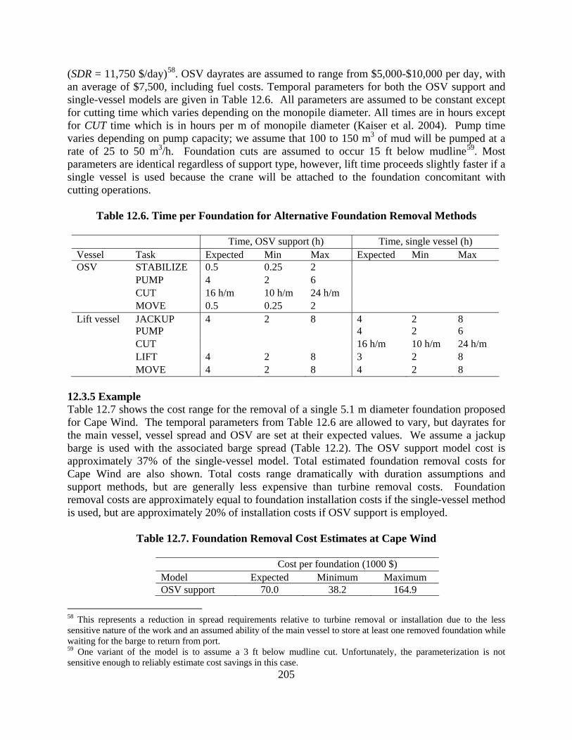
205

(SDR = 11,750 $/day)58. OSV dayrates are assumed to range from $5,000-$10,000 per day, with an average of $7,500, including fuel costs. Temporal parameters for both the OSV support and single-vessel models are given in Table 12.6. All parameters are assumed to be constant except for cutting time which varies depending on the monopile diameter. All times are in hours except for CUT time which is in hours per m of monopile diameter (Kaiser et al. 2004). Pump time varies depending on pump capacity; we assume that 100 to 150 m3 of mud will be pumped at a rate of 25 to 50 m3/h. Foundation cuts are assumed to occur 15 ft below mudline59. Most parameters are identical regardless of support type, however, lift time proceeds slightly faster if a single vessel is used because the crane will be attached to the foundation concomitant with cutting operations.

Table 12.6. Time per Foundation for Alternative Foundation Removal Methods

Time, OSV support (h) Time, single vessel (h) Vessel Task Expected Min Max Expected Min Max OSV STABILIZE 0.5 0.25 2 PUMP 4 2 6 CUT 16 h/m 10 h/m 24 h/m MOVE 0.5 0.25 2 Lift vessel JACKUP 4 2 8 4 2 8 PUMP 4 2 6 CUT 16 h/m 10 h/m 24 h/m LIFT 4 2 8 3 2 8 MOVE 4 2 8 4 2 8

12.3.5 Example Table 12.7 shows the cost range for the removal of a single 5.1 m diameter foundation proposed for Cape Wind. The temporal parameters from Table 12.6 are allowed to vary, but dayrates for the main vessel, vessel spread and OSV are set at their expected values. We assume a jackup barge is used with the associated barge spread (Table 12.2). The OSV support model cost is approximately 37% of the single-vessel model. Total estimated foundation removal costs for Cape Wind are also shown. Total costs range dramatically with duration assumptions and support methods, but are generally less expensive than turbine removal costs. Foundation removal costs are approximately equal to foundation installation costs if the single-vessel method is used, but are approximately 20% of installation costs if OSV support is employed.

Table 12.7. Foundation Removal Cost Estimates at Cape Wind

Cost per foundation (1000 $) Model Expected Minimum Maximum OSV support 70.0 38.2 164.9

58 This represents a reduction in spread requirements relative to turbine removal or installation due to the less sensitive nature of the work and an assumed ability of the main vessel to store at least one removed foundation while waiting for the barge to return from port. 59 One variant of the model is to assume a 3 ft below mudline cut. Unfortunately, the parameterization is not sensitive enough to reliably estimate cost savings in this case.

206

Single-vessel 345.9 211.1 545.5 Total costs (1000 $) OSV support 9,100 4,966 21,437 Single-vessel 44,967 27,443 70,915

12.4 Cable

Cable removal cost estimation procedures are identical for export and inner-array cables. Removal cost is estimated based on the length of cable (in km) divided by the rate of cable removal (in km/d), times the total vessel daily cost ($/d). If cable length is known it may be input into the model; otherwise, distance to shore may be used as a proxy for export cable and inner-array length may be approximated via formula60. Vessel requirements for cable removal are less severe than those for cable installation61 and we assume that low cost vessels, specifically tugs, barges, mechanical dredges and OSVs, will be utilized. In removal, the cable is expected to be cut in several small sections. In general, the ability to remove cable without dredging or jetting depends on the weight and length of the cable, the sediment type, and the capacity of the winch. Vessels with large turntables and ROVs are not required in removal operations. 12.4.1 Parameterization Cable removal time is estimated from the installation rate (km/day) and an inflation factor (IF); IF = 1 indicates that installation and removal occur at the same rate; IF = 2 indicates that removal proceeds twice as fast as installation. For inner-array cables, IF is assumed to range from 1.5 to three, and for export cables, IF ranges from one to two. Installation rates generally range from 0.1 to 0.6 km/d (0.3 km/d average) for inner-array cables and 0.2 to 1.4 km/d (0.7 km/d on average) for export cables. For inner-array cables, the total daily cost is composed of barge spread and OSV cost; diving operations are expected to be supported by the OSV. OSVs are assumed to be large and to cost 15,000 to 25,000 $/day (average $20,000/d) and a barge spread is assumed to cost 7,000 to 17,000 $/day (average $12,000/d). For export cables, an extra vessel is required to help retrieve buried sections of cable. A variety of vessels could complete this task (e.g. OSV, specialized barge spread, dredge spread) and we assume an additional 15,000 $/day is required. 12.4.2 Example Table 12.8 summarizes estimated cable removal costs at Cape Wind. Cable length is taken from company estimates (MMS 2008; Pirelli and ABB 2004). The maximum and minimum costs in Table 12.8 are generated by varying the inflation factor between its maximum and minimum values and leaving all other parameters at their expected values.

60 For example, inner-array cable length (km) is correlated with farm capacity (FC, MW) by:

. 61 Cable laying is more difficult than cable removal due to the vessel requirements and the need to lay cables in a single continuous piece and to bury the cable.

207

12.5 Substation and Met Tower

Substation decommissioning consists of a topside removal plus jacket removal. A heavy-lift vessel will be required to lift the topsides from the jacket and place it on a barge. The same vessel will then perform the jacket lift after the foundation piling has been cut. If the foundation piling is grouted into the jacket legs, the foundation and piling will be lifted together. An OSV will be required to support divers and pile cutting operations and it is expected that the OSV and heavy-lift vessel will remain on site throughout the operation. Therefore, the daily cost consists of the heavy-lift vessel, OSV and barge spread costs, at a total cost between $122,000 and $140,000 per day. Table 12.9 shows the estimated time of the operation.

Table 12.8. Cable Removal Cost Estimates at Cape Wind

Cable type (unit) Calculation Inner-array Export Length (km) Input 130 25 Installation time (km/d) Input 0.3 0.7 Inflation factor Input 2 1.25 Removal rate (km/d) Installation time * Inflation factor 0.6 0.9 Removal time (d) Length ÷ Removal rate 217 28 Total dayrate ($/d) Input 32,000 44,000 Expected cost (1,000 $) Removal time * Total dayrate 6,944 1,232 Maximum cost (1,000 $) Removal time * Total dayrate 9,244 1,571 Minimum cost (1,000 $) Removal time * Total dayrate 4,622 783

A met tower will undergo a similar process but with smaller, less expensive vessels. We assume that a large liftboat or jackup barge and barge spread are mobilized to the site. The topsides are disassembled and placed on a barge and the piles are cut with support from crew on the liftboat. We assume that the daily cost ranges from 47,000 to 76,000 $/day. The daily cost includes 35,000 to 64,000 $/day for a liftboat or jackup and 12,000 $/day for a barge spread. The temporal components are shown in Table 12.9.

Table 12.9. Temporal Components of Substation and Met-Tower Removal

Activity Substation (h) Met tower (h) TRANSIT 12 12 PLACE ANCHOR 1 1 CUT TOPSIDES 12 4 LIFT TOPSIDES 3 3 CUT PILES 48 36 LIFT JACKET 3 3 PULL ANCHOR 1 1 TRANSIT 12 12 TOTAL TIME 92 72 Expected cost (1,000 $) 502 185 Maximum cost (1,000 $) 536 228 Minimum cost (1,000 $) 467 141

208

Substation and met tower removal cost are estimated to range between $467,000 to $536,000 and $141,000 to $185,000, respectively.

12.6 Scour Protection

Scour protection removal may occur before foundation removal (if an external cut is required) or following foundation removal. A mechanical dredge is required to lift rock armor onto a cargo barge; for concrete mattresses dredging methods and costs are likely to be different. Dredging costs for all U.S. Army Corps of Engineer funded projects are analyzed annually and are approximately $5 per cubic yard (including material disposal). However, non-hopper and work similar to scour protection removal can be more expensive, averaging $23 per cubic yard, with some individual projects costing up to $104 per cubic yard (USACE 2010). Given the density of scour protection and the complications of the marine environment, we assume a removal cost of $25 per cubic yard ($33 per m3). Each turbine is assumed to be protected with 1000-1500 tons of rock armor. Metamorphic rock has a density of approximately 2.75 g/cm3 (Smithson 1971); therefore, each foundation is protected by 363 to 545 m3 of rock62. Given these assumptions, removal cost is expected to range between $12,000 and $18,000 per foundation.

12.7 Site Clearance

Site clearance can be conducted across the entire farm or on a per turbine basis. That is, the entire area of the farm could be trawled, or just the area around each turbine to some set radius. Current regulations are defined in terms of a structure basis but the radius of clearance has not been specified. We consider both cases. 12.7.1 Per-Turbine If site clearance operations for wind turbines are similar to caisson and well-protector site clearance in the oil and gas industry and have a similar level of debris removal,63 then empirical data from the oil and gas industry can be used to infer site clearance cost in offshore wind. We assume that the area to a radius of 183 m centered at each turbine will be trawled. Since turbine spacing is typically on the order of seven turbine diameters, the clearance zones would not overlap. We assume that site clearance is approximately $16,000 per foundation (range $6,000 to $26,000; Kaiser and Martin 2009) and the total cost is determined from the number of turbines, substations and met towers times the cost per turbine. 12.7.2 Whole Farm For the entire wind farm, the total project cost is the farm area times the cost per unit area. The area of the wind farm can be input by the user if known or may be estimated via formula64. Site clearance and verification cost is assumed to be 84,000 $/km2 (range 37,000 to 131,000 $/km, Kaiser and Martin 2009); this is the unit cost for oil and gas platforms, however, because the area

62 This is consistent with the 380 m3 of scour placed around the turbines at the Horns Rev 2 wind farm. 63 This is believed to be a reasonable assumption because maintenance and repair operations will mostly occur inside the tower and nacelle assemblies and offshore turbines are unmanned facilities similar to caissons and well protectors. 64 For example, farm area is given by: where AREA is described in square km, RD is the rotor diameter (m), and NT is the number of turbines.

209

of a wind farm is significantly greater than the area of a platform, and the cleanup vessels are on-site and primed for work, we expect some savings due to economies of scale. 12.7.3 Example Application of the site clearance and verification cost algorithm is illustrated for Cape Wind in Table 12.10. The costs of per-turbine clearance are similar but less than the costs of whole farm clearance because the clearance area is smaller, about 23% of the total farm area. Costs range from approximately $1 million to $3.5 million with an expected value of $2 million. These costs may overestimate actual cost due to cheaper dayrates associated with the long term charter of a vessel. Site clearance costs are expected to be a small but non-negligible proportion of removal costs.

Table 12.10. Estimated Site Clearance and Verification Costs at Cape Wind

Model Parameterization Unit Cost Number units

Estimated costs (1000 $)

Per turbine Expected 16,000 $/turbine 132a 2,112 Per turbine Minimum 6,000 $/turbine 132a 792 Per turbine Maximum 26,000 $/turbine 132a 3,432 Whole site Expected 43,000 $/km2 62 km2 2,399b Whole site Minimum 19,000 $/km2 62 km2 1,060b Whole site Maximum 67,000 $/km2 62 km2 3,739b Note: a. includes one met tower and one substation.

b. includes 10% economy of scale discount

12.8 Material Disposal Costs

Disposal costs consist of three components: processing costs, transport costs and scrap profits or landfill costs. There are several disposal options for wind farm components (Table 12.11) and the ultimate disposition of each component will determine total cost.

Table 12.11. Disposal Options by Component

Component Reef Landfill Scrap Leave in place Turbine blades N Y N N Turbine nacelle N Y Y N Turbine tower N U Y N Monopile-transition piece assembly Y Y Y N Monopile Y U Y N Cables N Y N Y Scour protection N U Y Y Substation foundation Y U Y N Substation topsides N Y N N U = Unlikely

210

12.8.1 Processing Costs Material to be scrapped or landfilled incurs processing costs. For landfilled material, processing consists of cutting the pieces into lengths and weights transportable by truck (assumed to be under 40 feet long and under 20 tons). For scrap steel, processing will involve cutting pieces into suitable sizes to be accepted by mini-mills (typically 2 ft x 5 ft). Processing costs may be estimated on either a per foot or per ton basis. There are a variety of methods which may be used to cut monopiles, towers and the monopile/transition piece assembly. The cost to cut tubular steel is determined by local labor expense, the complexity of the cut, thickness of the steel, and the cutting method employed (Kaiser and Pulsipher 2010). A variety of tools may be used to make cuts including oxyfuel torches, thermal lances, abrasive water jets and plasma arcs. We assume that thermal lances will be used due to the material thickness and assumed lack of mechanized cutting facilities. Table 12.12 shows cut time and costs for monopiles, towers and monopile/transition piece assembly. We assume a labor cost of 25 $/h. To determine the total length of cut required to decompose a tubular member into pieces that can be accepted by a mini-mill, we use:

(12-18)

where D is the diameter, C is the circumference, and L is the length of the tubular member, and X and Y is the length and width dimension of a final cut piece, respectively65. Domestic heavy metal steel (HMS) #1 accepted by mini-mills is at least ¼ inch thick and no larger than 5 ft × 2 ft. Lengths and diameters may be input or estimated from the algorithms in Chapter 11.

Table 12.12. Estimated Onshore Component Cutting Costs Cost ($/ft) Component Thickness (cm) Cut rate (cm/s) Material Labor Total Tower 3 0.5 3 0.4 3.4 Monopile 5 0.2 8 1.1 9.1 Monopile/transition* 5 + 7+ 5 0.2, 0.15, 0.2 8 + 10 +8 3.6 29.6 Note: * composed of steel, grout, steel Source: Wang et al., 2004 a & b We assume that the cost of removing the grout from the monopile/transition piece is $20/ton. For processing of substation jackets we assume a cost of 50 to 100 $/ton (Kaiser and Pulsipher 2010). We assume turbine and substation topside processing will be relatively complex and will cost 100-200 $/ton. 12.8.2 Scrap Value Steel is a highly recyclable material that can be sold at a resale value determined by the regional scrap steel price. The value of scrap steel is determined by its weight, quality, size, and the

65 The operators indicate round up and round down, respectively; min indicates the component with the smaller value should be selected.

211

regional supply-demand conditions at the time of sale. The costs of heavy metal scrap HMS #1 steel from 2005 to 2010 are shown in Figure 12.2. The average price over the period was 243 $/t. We assume an average scrap value of 243 $/t with a range of 100 to 380 $/t. 12.8.3 Landfill Cost We define landfill costs as the costs to dispose of anything that is not recycled, reefed, or left in place. We assume that landfilled materials all fit into the category of “construction and demolition” or inert waste. While some hazardous material such as oil and electronic components exist in turbines, they are ignored. Landfill costs for inert and demolition waste material are variable, and we assume they range from 20 to 136 $/ton with an expected cost of 30 $/t (Georgia Department of Community Affairs 2010; Elzarka 2007; Araman et al. 1997). Landfill costs vary regionally and are expected to be lowest in the Southeast and Gulf and highest in the Northeast and Mid-Atlantic States. Figure 12.2. U.S. Heavy Metal Steel Scrap Price

Source: Steel Business Briefing 12.8.4 Transport Costs Both scrap and landfill material must be transported by truck from port to a waste facility. Total transport costs and the transport unit cost are a function of transport distance. Mini-mills are disproportionately located in Gulf, Atlantic, and Great Lake states, particularly Pennsylvania, Texas, South Carolina, New York, New Jersey, Indiana, Illinois and Ohio. We assume a transport cost of 1.6 to 2.4 $/mi (Fairtran 2010) and that a truck carries 24 tons, giving a cost per ton-mile of 0.07 to 0.1 $, with an expected cost of 0.08 $/t-mi. A 200 t turbine tower transported 400 mi to a mini-mill, for example, would cost 0.08 $/t-mi * 200 t * 400 mi = $6,400. Transport costs are small relative to other costs. 12.8.5 Reefing If a reef site can be identified and permitted close to the wind farm, it is possible that reefing will be performed for its ecological value and to reduce disposal, processing and transport costs. If a reef site is further from the wind farm than the distance to port, additional transport cost will be

212

incurred and reefing may not be economic. Since we know neither the distance to port nor the distance to a hypothetical artificial reef, we assume the distances are equal and transport costs are ignored. The total costs of reef disposal, including processing, transport, and landfill costs are assumed to be zero. 12.8.6 Example Table 12.13 shows the expected disposal costs at Cape Wind. We assume the free monopile, monopile/transition piece assembly, and tower are 35, 30 and 225 ft long, respectively. We assume the transport distance is 100 mi and we use the length and weight algorithms presented in Chapter 11. Due to the low cutting costs and large weight, the tower provides the greatest profit. However, even with higher processing costs, the monopile/transition piece assembly can be sold for revenue, suggesting that given this combination of parameters, reefing will not be undertaken. The non-recovered portion of the turbine provides the greatest costs suggesting that economies may be achieved by maximizing the proportion of the turbine recovered. In our model, cables are always costly to dispose of and we expect that in many cases they will be left in place.

12.9 Cape Wind Decommissioning Scenarios

Table 12.14 shows three scenarios for decommissioning operations at Cape Wind. In the first scenario, the cable and scour protection is removed; in the second scenario, cable and scour protection is left in place. In the third scenario, the turbine felling option is employed. The first two scenarios are parameterized with expected values. In both cases the costs are similar and the majority of costs are due to turbine removal. We assume that foundation cutting will be performed by an OSV; if a heavy-lift vessel is required, the total decommissioning costs increase by approximately $35 million and foundation removal becomes as expensive as turbine removal. In both scenarios, it is the removal costs rather than the disposal costs that drive overall decommissioning costs. Overall costs are approximately 100,000 to 140,000 $/MW; these costs are less than 5% of the total capital costs (estimated at 3.6 million $/MW). The turbine felling option is also depicted. Under felling, the turbine removal costs decline from $48.7 to $22.1 million. The range of turbine removal costs using the felling technique is $8.8 to $35.1 million; even in the maximum parameterization felling is less expensive than the expected costs via standard methods. This suggests that the felling option will be a less expensive alternative to standard decommissioning methods if technical obstacles are overcome.

12.10 Decommissioning Costs at Proposed Offshore Wind Farms

Table 12.15 shows decommissioning costs at three proposed U.S. offshore wind farms: Coastal Point (TX), Bluewater Wind (DE), and Garden State (NJ). Input data on the expected system configurations are obtained from public sources, but because of the early stages of development, the input is considered more uncertain than Cape Wind, and thus, the output results will be similarly limited. Turbines are assumed to be removed by SPIV via the self-transport method. Foundations are removed by OSV support, cables and scour are left in place, and expected values are used for all

213

parameterizations. Two of the projects plan to use jacket or tripod foundations rather than monopiles; we model removal costs for these projects as if they were monopiles and ignore scrap income. Estimated decommissioning costs at the three projects ranged from 129,000 to 156,000 $/MW, consistent with estimates for Cape Wind. As in Cape Wind, removal costs were the dominant driver of total cost, and turbine removal accounted for approximately 80% of removal costs. The model output is insensitive to changes in weight, length and diameter assumptions, but is sensitive to changes in assumptions that impact turbine removal time.

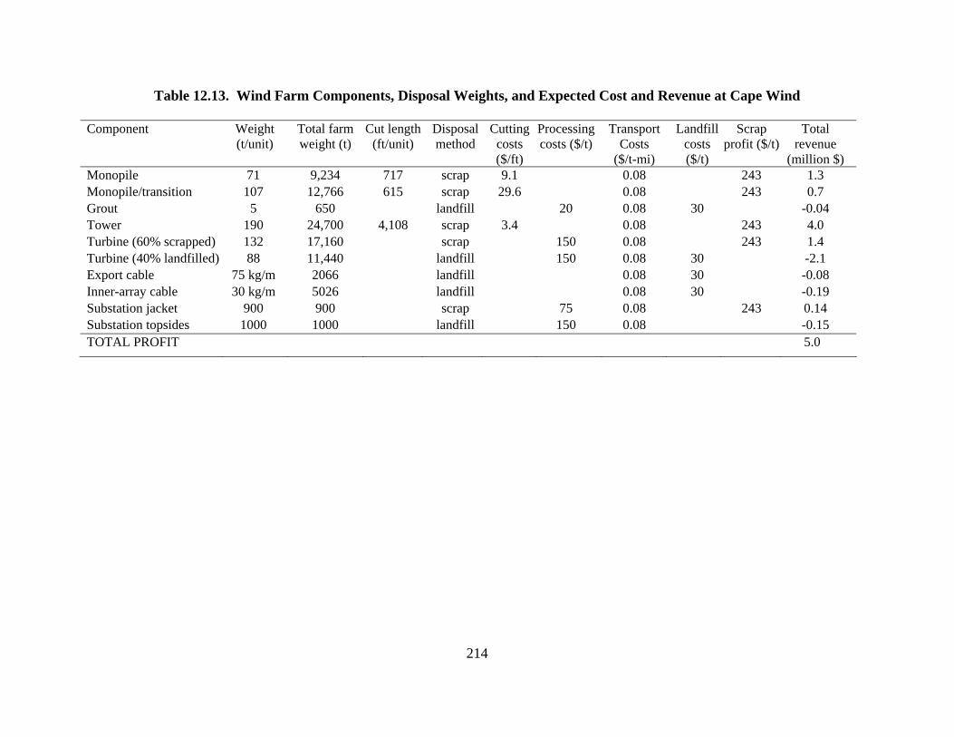
214

Table 12.13. Wind Farm Components, Disposal Weights, and Expected Cost and Revenue at Cape Wind

Component Weight (t/unit)

Total farm weight (t)

Cut length (ft/unit)

Disposal method

Cutting costs ($/ft)

Processing costs ($/t)

Transport Costs

($/t-mi)

Landfill costs ($/t)

Scrap profit ($/t)

Total revenue

(million $) Monopile 71 9,234 717 scrap 9.1 0.08 243 1.3 Monopile/transition 107 12,766 615 scrap 29.6 0.08 243 0.7 Grout 5 650 landfill 20 0.08 30 -0.04 Tower 190 24,700 4,108 scrap 3.4 0.08 243 4.0 Turbine (60% scrapped) 132 17,160 scrap 150 0.08 243 1.4 Turbine (40% landfilled) 88 11,440 landfill 150 0.08 30 -2.1 Export cable 75 kg/m 2066 landfill 0.08 30 -0.08 Inner-array cable 30 kg/m 5026 landfill 0.08 30 -0.19 Substation jacket 900 900 scrap 75 0.08 243 0.14 Substation topsides 1000 1000 landfill 150 0.08 -0.15 TOTAL PROFIT 5.0

215

Table 12.14. Decommissioning Cost Summary at Cape Wind With Cable Removal

(million $) Without Cable Removal

(million $) Stage Component Cost Revenue Cost Revenue Removal Turbines (felling option) 48.7 (22.1) 48.7 (22.1) Foundations 9.1 9.1 Substation 0.5 0.6 Cable - export 1.2 Cable - inner-array 6.9 Met tower 0.2 0.3 Scour 1.9 Site clearance 2.1 2.1 Removal sub-total (felling option) 70.5 (43.9) 60.6 (34.0) Disposal Turbine - nacelle and blades 1.4 1.4 Turbine - tower 4.0 4.0 Foundation 2.0 2.0 Substation-jacket 0.14 0.14 Substation –topsides 0.15 0.15 Cable - export 0.08 Cable - inner-array 0.19 Disposal sub-total 0.6 7.4 0.3 7.4 TOTAL COST (felling option) 63.8 (37.2) 53.5 (26.9)

Table 12.15. Decommissioning Costs at Proposed U.S. Windfarms Windfarm Capacity

(MW) Number

of turbines

Distance to port (nm)

Removal costs

(million $)

Disposal costs

(million $)

Scrap revenue

(million $)

Total cost (million $)

Coastal Point, TX* 150 60 20 24.5 0.9 1.9 23.4 Bluewater, DE 450 150 100 68.3 1.7 10.3 59.7 Garden State, NJ* 350 96 80 47.7 1.8 4.2 45.3

* Projects to use tripod/jacket foundation.

12.11 Discussion

12.11.1 Proposed U.S. Wind Farms Bonding Requirements Bonding requirements for offshore wind farms are most accurately estimated on a case-by-case basis using models like those presented here. It would be inappropriate to determine bonding requirements on a per MW or per turbine basis as decommissioning costs are dependent on the turbine size and capacity, the number of turbines, foundation type, methods of removal, methods of disposal and the components allowed to remain in place. In most cases, we expect decommissioning liability to be about 5-10% of the capital costs of the wind farm. From a regulatory perspective, it is important that operators remain a going concern

216

and generate enough income to satisfy decommissioning requirements at the end of the lease. In the offshore oil and gas industry, an important measure of the capability of an operator to meet their decommissioning obligations is the ratio of reserves in place or annual income to their decommissioning liability (Kaiser 2010). In offshore wind, the equivalent measures would be the value of power generated over the life of the farm (reserves in place) or annually. Power purchase agreements (PPA) are finalized before construction begins, and capacity factors can be reliably estimated from wind speed data. Therefore, unlike oil and gas development, the income of the developer may be reliably forecast well into the future. This should serve to reduce uncertainty associated with default of the operator. For example, Cape Wind signed a PPA with the local grid operator for 0.187 $/kWh and expects a capacity factor of 36%; the term of commercial operations is expected to be 25 years. This gives an annual income of approximately $275 million and a lifetime income of $6.9 billion, far greater than the decommissioning liability. In the offshore oil and gas industry, operators meeting certain financial capability tests are not required to post decommissioning bonds. The Code of Federal Regulations contains no such exception for offshore wind operations, however, such a regulation may be appropriate for some corporations interested in offshore development. For example, Bluewater Wind is a subsidiary of NRG, a company with over $5 billion in market capitalization, and Southern Company, a potential developer of sites off the Southeast coast has a market capitalization of over $30 billion. 12.11.2 Limitations Decommissioning cost models are limited by the need to project current costs and technologies into the future and the development status of a project. While prices may be adjusted for an expected inflation rate, steel prices and vessel dayrates are highly uncertain and have significant direct and indirect impacts on costs. Due to these uncertainties, the range of all model parameters is large. As uncertainties propagate and interact through the calculations, the range of cost outputs increases. Removal technologies are not expected to change dramatically over the time periods considered, however, and so under a traditional scenario changes due to technological improvements are considered to be minor. Novel and creative methods of turbine removal, however, may significantly reduce total decommissioning cost. Some costs were not included in the cost estimates. Specifically, project engineering and management, and port rental were not included. We expect that these costs may add 10% to the total cost estimate.

217

REFERENCES

4COffshore. 2010. Database of Offshore Wind Projects. Lowestoft, UK. Alpha Ventus. 2010. Alpha Ventus. Available at

http://www.alpha-ventus.de/index.php?id=80 Accessed 10-26-2010. Ampelmann. 2010. Ampelmann assists offshore wind turbine installation in the North Sea.

Available from http://www.ampelmann.nl/index.php?id=106. Accessed 11-10-2010.

Araman, P.A., R.J. Bush, A.L. Hammet, and E.G. Hager. 1997. Wood pallets and landfills: Status and opportunities for economic recovery and recycling, In: Proceedings, WASTECON/ISWA World Congress, SWANA 36th Annual International Solid Waste Exposition, October 26-29, 1998, Charlotte, NC. Solid Waste Association of North America. Silver Spring, MD.

Atlantic Wind Connection. 2010. AWC schematic. Available at

http://atlanticwindconnection.com/news/awc-schematic. Accessed 11-10-2010. AWS Truewind. 2009. Offshore wind technology overview. New York-Long Island Offshore

Wind Collaborative. 9998. Bailey, J.E., C.W. Sullivan, and D. Cruise. 2010. Offshore Drilling Monthly. Houston, TX:

Jefferies and Company. Barthelmie, R., S. Frandsen, C. Morgan, T. Henderson, H.C. Sorensen, C. Garcia, G. Lemonis,

B. Hendriks, and B. O’Gallachóir. 2001. State of the art and trends regarding offshore wind farm economics and financing. Presented at the EWEA Special Topic Conference, Brussels, December 10-12, 2001.

Belwind. 2010. Facts and Figures. Available at

http://www.belwind.eu/index.php?page=feiten&lang=en Accessed 10-26-2010.

BERR. 2007a. Offshore wind capital grants scheme. Barrow Offshore Wind Farm 1st annual

report. London. 09/P45. Available at http://webarchive.nationalarchives.gov.uk/+/http://www.berr.gov.uk/files/file50163.pdf Accessed 10-24-2010.

BERR. 2007b. Offshore wind capital grants scheme. Kentish Flats Offshore Wind Farm 2nd

annual report. London 09/P46. Available at http://www.decc.gov.uk/assets/decc/what%20we%20do/lc_uk/ic_business/env_trans_fund/wind_grants/file50164.pdf Accessed 10-24-2010.

218

Bird, L., M. Bolinger, T. Gagliano, R. Wiser, M. Brown, and B. Parsons. 2005. Policies and market factors driving wind power development in the United States. Energy Policy 33: 1397-1409.

Bishop I.D. and D.R. Miller. 2007. Visual assessment of offshore wind turbines: The influence

of distance, contrast, movement and social variables. Renewable Energy 32: 814-831. Blackwell, B. 2009. DONG energy snaps up contracts for Walney. RechargeNews.com. June

30, 2009. Available at http://www.rechargenews.com/business_area/finance/article182126.ece?print=true Accessed 10-24-2010.

Bluewater Wind. 2010. Delaware. Internet website:

http://www.bluewaterwind.com/delaware.htm Accessed 10-24-2010. BOEMRE. 2010. BOEMRE map gallery. Available at

http://www.boemre.gov/offshore/mapping/gallery.htm. Accessed 11-12-2010 Bogo, J. 2010. Texas to Cape Wind; you’re not first yet. Popular Mechanics, May 3, 2010. BoWind. 2008. Construction. Available at http://www.bowind.co.uk/construction.shtml.

Accessed 11-10-2010. Bradbury, J. 2009. Jumbo joins up Greater Gabbard. Offshore Media Group. Available at

http://www.offshore247.com/news/art.aspx?Id=16602. Accessed 10-24-2010. BSH. 2010. North Sea: offshore wind farms. Available at

http://www.bsh.de/en/Marine_uses/Industry/CONTIS_maps/NorthSeaOffshoreWindfarmsPilotProjects.pdf Accessed 11-10-2010.

C-Power. 2010. Investment. Available at http://www.c-power.be/English/investment/index.html.

Accessed 10-26-10. Cape Wind. 2010. News. Available at http://www.capewind.org/Topics.htm. Accessed 10-29-

2010. CBP. 2010. Customs Ruling Online Search System. Available at http://rulings.cbp.gov/

Accessed 10-29-2010. Carter, M. 2007. North Hoyle offshore wind farm: design and build. Institution of Civil

Engineers, Proceedings, Energy 160(1): 21-29. Centrica. 2010. Renewables. Available at

http://www.centrica.com/index.asp?pageid=923#project4. Accessed 11-10-2010. Chatterton, A. 2004. Scroby Sands. UK Offshore Wind 2004, March 3-4, London.

219

Cole, J.C., R.P. Herrmann and R.J. Scott. 1997. Discoverer Enterprise: World's Most Advanced

Drilling Unit. SPE/IADC Drilling Conference, 4-6 March 1997, Amsterdam, Netherlands. 37659-MS.

Colton, T. 2010. Shipbuilding history. Available at http://shipbuildinghistory.com/. Accessed

10-29-2010. Coastal Point Energy. 2010. Introduction to Coastal Point Energy. Available at

http://www.millergroupofcompanies.com/presentations/CoastalPointEnergyPPT3.pdf. Accessed 10-29-2010.

Crown Estate. 2010. Offshore wind energy. Available at

http://www.thecrownestate.co.uk/offshore_wind_energy. Accessed 11-10-2010. Cruz, A.M. and E. Kraussman. 2008. Damage to offshore oil and gas facilities following

Hurricanes Katrina and Rita: An overview. Journal of Loss Prevention in the Process Industries 21(6): 620-626.

Culwell, A.S. and J. McCarthy. 1998. Pipeline and power cable decommissioning, In: Manago,

F. and B. Williamson, eds. Proceedings: Public Workshop, Decommissioning and Removal of Oil and Gas Facilities Offshore California: Recent Experiences and Future Deepwater, September 1997. MMS OCS Study 98-0023: 66-73.

de Alegría, I., J. Martín, I. Kortabarria, J. Andreu, and o. P. Ere. 2009. Transmission alternatives

for offshore electrical power. Renewable and Sustainable Energy Reviews, 13(5), 1027-1038.

De Jong, E. 2010. Ready for a heavy-lift of the share price. SNS Securities. De Vries, E. 2007. North Sea construction: Installing the monopiles for the Dutch Q7 offshore

wind farm. Renewable Energy World, May 1, 2007. Den Boon,J.H., J. Sutherland, R. Whitehouse, R. Soulsby, C.J.M. Stam, K. Verhoeven, M.

Høgedal, and T. Hald. 2004. Scour behaviour and scour protection for monopile foundations of offshore wind turbines. European Wind Energy Conference, November 22-25, London.

Deepwater Wind. 2010. Projects. Available at http://dwwind.com/projects. Accessed 10-29-

2010. Department of the Interior, Minerals Management Services. 2009. Renewable Energy and

Alternate Uses of Existing Facilities on the Outer Continental Shelf. Federal Register 74 (81): 19638-19871. April 29. To be codified at 30 CFR Parts 250, 285, and 290. (“MMS Final Rules”).

220

DOE. 2008. 20% wind energy by 2030. U.S. Department of Energy, Washington, D.C. DOE. 2010. How wind turbines work. Available at

http://www1.eere.energy.gov/windandhydro/wind_how.html. Accessed 11-12-2010. DONG Energy. 2007. Annual Report. Available at

http://www.dongenergy.com/EN/Investor/reports/Pages/annual%20reports2.aspx. Accessed 10-26-2010. DONG Energy. 2008. Annual Report. Available at

http://ipaper.ipapercms.dk/DONGENERGY/Internet/UK/Annualreports/AR2008UK/. Accessed 10-26-2010. DONG Energy. 2009a. Annual Report. Available at

http://www.dongenergy.com/EN/Investor/reports/Pages/annual%20reports2.aspx. Accessed 10-26-2010. DONG Energy. 2009b. DONG Energy sells minority stake in Walney Offshore Wind Farm.

Available at http://www.dongenergy.com/Walney/News/data/Pages/DONGEnergysellsminoritystakeinWalneyOffshoreWindFarm.aspx.

Accessed 10-24-2010. DONG Energy. 2009c. Gunfleet Sands notice to mariners. Available at

www.benfleetyachtclub.org/.../Gunfleet_Wind_Farm_Weekly_Notice_No._043.pdf. Accessed 11-10-2010.

DONG Energy. 2010a. Photo Archive. Available at

http://www.dongenergy.com/Nysted/EN/About_us/Photos/Pages/Photos.aspx. Accessed 11-12-2010.

DONG Energy 2010b. Horns Rev 2-Images. Available at

http://www.dongenergy.com/hornsrev2/en/images_/images_/pages/images_october_2008.aspx. Accessed 11-12-2010.

DONG Energy 2010c. Gunfleet Sands. Available at

http://www.dongenergy.com/Gunfleetsands/GunfleetSands/AboutGFS/Pages/default.aspx. Accessed 11-12-2010.

DONG Energy. 2010d. Walney offshore wind farm. Available at

http://www.dongenergy.com/Walney/Pages/index.aspx. Accessed 10-24-2010. Douglas Westwood and ODE. 2005. Scroby Sands supply chain analysis. Department of Trade

and Industry, London. 334-04

221

Drydocks World. 2010. Jack-up construction vessel. Available at http://www.drydocks-sea.com/services-offshore_wind.html. Accessed 11-10-2010.

DTI. 2004. The World offshore renewable energy report 2004-2008. Department of Trade and

Industry. London. URN 04/393CD. Elsam. 2002. Horns Rev Newsletter. Available at

http://www.hornsrev.dk/Engelsk/nyheder/nyh_aug_02/uk-aug_02.htm. Accessed 11-10-2010.

Elzarka, H. 2007. Making the case for construction waste management. International

Proceedings of the 43rd Annual Conference of the Associated Schools of Construction. Flagstaff, AZ. April 2007.

EPA. 2000. Analysis of commercial marine vessels emissions and fuel consumption data.

Washington DC. EPA420-R-00-002. Ernst and Young. 2009. Cost of and financial support for offshore wind. Department of Energy

and Climate Change. London. URN 09D/534. Esber, B. 2004. Title XI Financing for Vessel and Shipyard Improvement Projects. MarineLink.

Available at http://www.marinelink.com/news/article/title-xi-financing-for-vessel-and-shipyard-improvement-projects/322695.aspx. Accessed 10-28-10.

European Investment Bank. 2010a. Bard I offshore wind farm. Available at

http://www.eib.org/projects/pipeline/2009/20090432.htm. Accessed 10-24-2010. European Investment Bank. 2010b. Belwind: EIB finances Europe’s largest offshore wind farm.

Available at http://www.eib.org/projects/news/eib-finances-europes-largest-offshore-wind-farm.htm. Accessed 10-24-2010.

European Investment Bank. 2010c. Global Tech I offshore wind farm. Available at

http://www.eib.org/projects/pipeline/2009/20090259.htm. Accessed 10-24-2010. European Investment Bank. 2010d. Sheringham Shoal offshore wind farm. Available at

http://www.eib.org/projects/pipeline/2009/20090481.htm. Accessed 10-24-2010. EWEA. 2009. Oceans of opportunity. European Wind Energy Association, Brussels. EWEA. 2009. Wind energy-the facts. Earthscan, London. Fairtran. 2010. Rates and indexes. Available at https://www.fairtran.com/fairtrans/Truckload-

Rate-Index.aspx. Accessed 10-24-2010. Fitzgerald, J. 2005. Wind farm off Wicklow opens. Irish Times, Dublin. May 5, 2005.

222

Garden State Offshore Energy. 2010. Southern New Jersey. Available at

http://www.gardenstatewind.com/?page_id=9. Accessed 10-24-2010. Garrad Hassan. 2009. UK offshore wind: charting the right course. British Wind Energy

Association, London. Georgia Department of Community Affairs. 2010. 2009 Annual solid waste report – Executive

Summary. Atlanta, GA. Available at http://www.dca.state.ga.us/development/research/programs/downloads/2009ExecutiveSummary.pdf. Accessed 10-24-2010.

Gerdes, G., A. Tiedmann, and S. Zeelenberg. 2006. Case study: European offshore wind farms-

A survey for the analysis of the experiences and lessons learnt. DENA. Gerwick, B. C. 2007. Construction of marine and offshore structures, Third edition. Taylor and

Francis, Boca Raton, FL. Green, J., A. Bowen, L.J. Fingersh, and Y. Wan. 2007. Electrical collection and transmission

systems for offshore wind power. Offshore Technology Conference. April 30-May 3 2007, Houston, TX. 19090-MS.

Hartley, K. 2006. The winds of change: EPC contracts for offshore wind farms. Monday

Business Briefing. May 24, 2006. Hau, E. 2006. Wind turbines: fundamentals, technologies, application, economics. Springer-

Verlag, Berlin. Hercules Offshore. 2010. 2009 annual report. Available at

http://phx.corporate-ir.net/phoenix.zhtml?c=192573&p=irol-reportsAnnual. Accessed 10-29-2010.

Hewson, T.A., and J.B. Stamberg. 2008. Beech Ridge Energy LLC financial assurance needs.

Prepared for Mountain Communities for Responsible Energy. October 7. Hornbeck Offshore. 2010. Proxy material and 2009 annual report. Available at

http://ir.hornbeckoffshore.com/phoenix.zhtml?c=132245&p=irol-reportsAnnual. Accessed 10-29-2010.

Howe, B. 2001. Cable properties. Neptune Power. Available at

http://neptunepower.apl.washington.edu/documentation/documentation.html. Accessed 10-24-2010.

IEA. 2005. Offshore wind experiences. International Energy Agency, Paris. IEA Wind. 2009. IEA wind energy annual report 2008. International Energy Agency, Paris.

223

Jayaram, A. and Royes. 2009. Offshore drillers: Normalize it. Credit Suisse. Jeppsson, J., P.E. Larsen and A. Larsen. Technical description of Lillgrund power plant.

Vattenfall. 218258-1. Jenkins, P.B. and A.L. Crockford. 1975. Drilling costs. SPE European Spring Meeting. April 14-

15, 1975. London. 5266-MS. Jha, A. 2008. Offshore wind turbines: extreme wind/wave risk and regulatory needs. AWEA

Offshore Wind Power Workshop. Wilmington, Delaware. Sep. 9, 2008. Kaiser, M.J. 2010. Gulf of Mexico decommissioning market outlook. Offshore Magazine

Webcast. Available at http://www.talkpoint.com/viewer/presentation.asp. Accessed 10-26-2010.

Kaiser, M.J. and J. Martin. 2009. An update on the cost of net trawling operations in the Gulf of

Mexico. Marine Policy 33 (1): 58-63. Kaiser, M.J. and A.G. Pulsipher. 2010. Scrap and storage markets in the Gulf of Mexico-III.

Process workflows and industry structure. Energy Sources, Part B: Economics, Planning, and Policy 5(3): 250-260.

Kaiser, M.J., A.G. Pulsipher, and R.C. Byrd. 2004. Model estimates abrasive cutting costs. Oil

and Gas Journal 102 (39): 44-47. Kaiser, M. J. and A.G. Pulsipher. 2008. A review and update of supplemental bonding

requirements in the Gulf of Mexico. U.S. Department of Interior, Minerals Management Service, Herndon, VA. TA&R study #600. 147 pp.

Kempton, W., P. Mandelstam, M. Mercurio, W. Musial, G. Watson, J. Uliman, and S. Stewart.

2009. Research and development needs for offshore wind. American Wind Energy Association, Offshore Wind Working Group.

Kempton, W., F.M. Pimenta, D.E. Vernon, and B.A. Collie. 2010. Electric power from offshore

wind via synoptic-scale interconnection. Proceedings of the National Academy of Science 107(16): 7240-7245.

Kooijman, H.J.T., M. de Noord, C.H. Volkers, L.A.H. Machielse, F. Hagg, P.J. Eecen, J.T.G.

Pierik, and S.A. Herman. 2001. Cost and potential of offshore wind energy on the Dutch part of the North Sea. EWEA Special Topic Conference Offshore Wind Energy, Brussels. December 10-12, 2001.

Kühn, M., W.A.A.M. Bierbooms, G.J.W. van Bussel, M.C. Ferguson, B, Göransson, T.T.

Cockerill, R. Harrison, L.A. Harland, J.H. Vugts, and R. Wiecherink. 1998. Opti-

224

OWECS Final Report Vol. 0: Structural and economic optimization of Bottom-Mounted Offshore wind energy converters - executive summary. Delft University of Technology. Delft, Netherlands. IW-98139R.

Lane, N. 2008. Issues affecting tidal, wave, and in-stream generation projects. Prepared for

Members and Committees of Congrress. CRS Report for Congress RL 338833. Larsen, J.H.M., H.C. Soerensen, E. Christiansen, S. Naef, and P. Vølund. 2005. Experiences

from Middelgrunden 40 MW offshore wind farm. Copenhagen Offshore Wind Conference. October 26–28, 2005.

Lemming, J.K., P.E. Morthorst, and N.E. Clausen. 2007. Offshore wind power experiences,

potential and key issues for deployment. Riso National Laboratory, Frederiksborgvej, Denmark. RISO-R-1673(EN).

Liftra. 2010. Transport frames. Available at

http://www.liftra.com/html/transport_frames_uk.html. Accessed 11-10-2010. Lindving, K. 2009. A2Sea News. Available from

www.a2sea.com/Admin/Public/DWSDownload.aspx?File=%2FFiles%2FFiler%2FNewsletters%2FA2SEA_NEWS_Spring_2009.pdf robin rigg prowse. Accessed 10-29-2010.

Logan, J. and S.M. Kaplan. 2008. Wind power in the United States: technology, Economic, and

policy issues. Congressional Research Service [CRS]. RL34546. Lundgren, K. 2009. Centrica to build $1.2 billion wind farm, team up with SocGen. Bloomberg,

NY: October 28, 2009. Available at http://www.bloomberg.com/apps/news?pid=newsarchive&sid=ateP2AcRakFI. Accessed 10-26-2010.

Manwell, J.F., C.N. Elkinton, A.L. Rogers, and J.G. McGowan. 2007. Review of design

conditions applicable to offshore wind energy systems in the United States. Renewable and Sustainable Energy Reviews 11: 210-234.

Manwell, J.F., J.G. McGowan and A.L. Rogers. 2002. Wind energy explained-theory, design

and applications. John Wiley and Sons, New York, NY. MARAD. 2010. Title XI Federal Ship Financing Program. Available at http://www.marad.dot.gov/ships_shipping_landing_page/title_xi_home/title_xi_home.ht

m. Accessed 10-29-2010. Marine Log. 2010. Aker Philadelphia eyes wind turbine installation vessels. Available at

http://www.marinelog.com/DOCS/NEWSMMIX/2010feb00220.html. Accessed 10-24-2010.

225

Master Marine. 2009. StatoilHydro and Statkraft have awarded a major contract to Master Marine. Available at http://www.master-marine.no/index.php?option=com_content&task=blogsection&id=1&Itemid=99. Accessed 10-24-2010.

Mastiaux, F. 2010. E.ON Offshore Wind Energy Factbook. E.ON, Düsseldorf, Germany

Available at: http://www.eon.com/en/downloads/EON_Offshore_Factbook_April_2010_EN.pdf. Accessed 10-24-2010.

May, J. 2009. North Hoyle and Rhyl Flats offshore wind farms: Review of good practice in

monitoring, construction and operation. Presentation to Scottish National Heritage, Inverness Scotland. July, 17, 2009.

Melnyk, M.M.W. and R.M. Andersen. 2009. Offshore Power. PennWell. Tulsa, OK. Middelgrundens Vindmollelaug. 2010. About Middelgrunden Wind Cooperative. Available at

http://www.middelgrunden.dk/middelgrunden/?q=en/node/35. Accessed 11-12-2010. Ministry of Foreign Affairs of Denmark. 2009. DONG Energy soon to inaugurate Horns Rev 2

offshore wind farm. Available at http://www.investindk.com/visNyhed.asp?artikelID=22253. Accessed 10-26-2010.

MMS. 2008. Cape Wind energy project: Final environmental impact statement. Minerals

Management Service. Herndon, VA. 2008-040. Moeller, A. 2008. Efficient offshore wind turbine foundations. Power Expo, Zaragoza, Spain,

September 24-25, 2008. Available at http://www.aeeolica.es/doc/powerexpo2008/06-Anders-Moller-DENSIT.pdf. Accessed 10-24-10.

Morgan, C.A., H.M. Snodin, and N.C. Scott. 2003. Offshore wind: economics of Scale,

engineering resource and load factors. Department of Trade and Industry. London. 3914/BR/01.

MPI. 2010. Lynn and inner dowsing wind farm. Available at http://www.mpi-

offshore.com/workboats-projects/lynn-and-inner-dowsing-offshore-wind-farm. Accessed 10-26-2010.

Musial, W.D. and C.P. Butterfield. 2004. Future for offshore wind energy in the United States.

NREL/CP-500-36313. EnergyOcean Proceedings. Palm Beach, FL, June 2004. Musial, W., S. Butterfield, and B. Ram. 2006. Energy from offshore wind: Preprint. Offshore

Technology Conference. Houston TX: NREL/CP-500-39450.

226

Musial, W. and B. Ram. 2008. Status of offshore wind energy projects, policies and programs in the United States. Presented at the 2007 European Offshore Wind Conference, Berlin. December 4–6, 2008. NREL/CP-500-42452.

Musial, W. and B. Ram. 2010. Large scale offshore wind power in the United States:

Assessment of opportunities and barriers. National Renewable Energy Laboratory. Golden, CO. NREL/TP-500-40745.

NordzeeWind. 2008. Offshore Wind Farm Egmond aan Zee General Report. Ijmuiden,

Netherlands. OWEZ_R_141_20080215. Available at http://www.noordzeewind.nl/files/Common/Data/OWEZ_R_141_20080215%20General%20Report.pdf. Accessed 10-24-2010.

ODE. 2007. Study of the costs of offshore wind generation. Department of Trade and Industry. Offshore Wind Power Marine Services. 2010. Gallery. Available at

http://www.offshorewindpower.co.uk/gallery.html. Accessed 11-12-2010. Offshore Shipping Online. 2000. Insurance deal makes tug-barge option attractive. August 25,

2000. Available at http://www.oilpubs.com/v_oso/print.asp. Accessed 10-29-2010. OilVoice. 2008. Subocean announces another multi-million pound offshore windfarm contract.

Oil Voice, London. September 17, 2008. Available at http://www.oilvoice.com/PrinterFriendly/Subocean_Announces_Another_Multimillion_Pound_Offshore_Windfarm_Contract/87adb104.aspx. Accessed 10-24-2010.

Penhale, G. 2008. Rhyl Flats offshore wind project delivery – a client’s perspective. BWEA 30th

Annual Conference. London, October 21-23, 2008. Pepper, L. 2001. Monitoring and evaluation of Blyth Offshore Wind Farm. Department of

Trade and Industry. London. DTI URN 01/686. Pirelli & ABB. 2004. Interstitial optical option for submarine composite cable. Available at

http://www.boemre.gov/offshore/PDFs/CWFiles/123.pdf. Accessed 10-24-2010. Poulsen, S.F. Efficient Installation of offshore wind turbines – lessons learned from Nysted

Offshore Wind Farm. Copenhagen Offshore Wind Conference. October 26-28. Puskar, F. 2010. Assessment of damage and failure mechanisms for offshore structures and

pipelines in Hurricanes Gustav and Ike. BOEMRE. Herdon, VA. TAR No.: 642. Prowse, M. 2009. Installation logistics for UK Round 3 wind farms. BWEA Offshore

Conference, Westminster, UK. June 24 -25. Prowse, M. 2006. A2Sea vessel support letter.

227

Prysmian. 2010. Prysmian will develop the power links for the Walney Offshore Wind Farm, in the Irish sea. Prysmian Energy. Milan. Jan 12, 2010.

Quillen, K. 2010. Stakes are high for Louisiana maritime industry in debate over decades-old

law. The Times-Picayune. New Orleans, LA. January 31, 2010. Ressin, C. 2009. Proposed modification and revocation of ruling letters relating to the Cutoms

position on the application of the Jones Act to the transportation of certain merchandise and equipment between coastwise points. U.S. Customs and Border Protection, Washington, DC. CBP Bulletins and Decisions. July 17, 2009.

Robinson, M. and W. Musial. 2006. Offshore wind technology overview. National Renewable

Energy Laboratory, Golden, CO. NREL/PR-500-40462. Available at http://www.nrel.gov/docs/gen/fy07/40462.pdf. Accessed 10-24-10.

Roddick, B.M. 1995. Towage insurance. Tulane Law Review (70): 679. SAL. 2010. MV "Annette" transports monopiles for the Walney Offshore Project. Available at

http://www.sal-heavylift.com/eng/news#jumpto-81. Accessed 11-10-2010. RWE npower. 2010. Rhyl Flats offshore wind farm picture gallery. Available at

http://www.rwe.com/web/cms/en/394364/rwe-npower-renewables/sites/projects-in-operation/wind/rhyl-flats/summary/picture-gallery/. Accessed 11-10-2010.

Schaumann, P., F. Wilke, and S. Lochte-Holtgreven. 2008 Nonlinear structural dynamics of

offshore wind energy converters with grouted transition piece. European Wind Energy Conference. Brussels. March 31- April 3, 2008.

Schellstede, H. 2008. Wind power: wind farms of the northern Gulf of Mexico. Paper presented

at Offshore Technology Conference, 30 April-3 May 2007. Houston, Texas. 19092-MS. Scottish and Southern Energy. 2010. Greater Gabbard . Available at

http://www.sse.com/SSEInternet/uploadedFiles/Media_Centre/Project_News/Greater_Gabbard/GG-plan.pdf. Accessed 11-10-2010.

Seidel, M. 2007. Jacket Substructures for the REpower 5M Wind Turbine. European Offshore

Wind Conference, December 4-6, Berlin. Semco. 2010. Photo gallery. Available at http://semcollc.com/semco_site_2_006.htm. Accessed

11-10-2010. Sheringham Shoal. 2010. Gallery. Available at

http://www.scira.co.uk/NewsDownloads/gallery.html. Accessed 10-28-2010. Smithson, S. 1971. Densities of metamorphic rocks. Geophysics, 36, 690.

228

Snyder, B. and Kaiser, M. J. 2009. Ecological and economic cost-benefit analysis of offshore wind energy. Renewable Energy (34):1567-1578.

Sørensen, H.C, Hansen, L.K., and Larsen, J.H.M. 2002. Middelgrunden 40 MW offshore wind

farm Denmark-Lessons learned. Renewable Realities – Offshore Wind Technologies. Orkney, UK. October 2002.

StatoilHydro 2009. StatoilHydro to build first full scale floating offshore wind turbine.

Available at http://www.statoil.com/en/NewsAndMedia/News/2008/Pages/hywind_fullscale.aspx. Accessed 11-12-2010.

StatoilHydro 2010. Press gallery. Available at

http://fotoweb.statoil.com/fotoweb/grid.fwx?archiveId=5004. Accessed 11-12-2010 Stromsta, K. 2010. Dong launches 172MW Gunfleet Sands offshore wind project.

Rechargenews.com. June 16, 2010. Available at http://www.rechargenews.com/energy/wind/article217994.ece?print=true. Accessed 10-26-2010.

Superior Energy Services. 2010. Quarterly report which provides a continuing view of a

company's financial position. Available at http://ir.superiorenergy.com/phoenix.zhtml?c=97570&p=irol-sec. Accessed 10-29-2010.

SWERA. 2010. Maps of Wind and Solar Energy. Available at

http://swera.unep.net/index.php?id=map_search&action_method=external_archive_query&datatype=70,79&geoarea=-1&energycategory=17&orderby=geoarea. Accessed 11-10-2010.

Talisman Energy. 2006. Images. Available at http://www.beatricewind.co.uk/press/event_1.asp.

Accessed 11-10-2010. Talisman Energy. 2007. The Beatrice Wind Farm Demonstrator – Fact Sheet.

Available at http://www.beatricewind.co.uk/press/facts.asp. Accessed 10-26-2010. Thresher, R., M. Robinson, and P. Veers. 2008. Wind energy technology: current status and

R&D future. Presented at the Physics of Sustainable Energy Conference University of California at Berkeley. March 1-2, 2008. NREL/CP-500-43374.

Tidewater. 2009. 2009 Annual Report. Available at

http://phx.corporate-ir.net/phoenix.zhtml?c=81406&p=irol-reportsannual. Accessed 10-29-2010.

Troll Windpower. 2009. Infield cable laying. Available at

http://www.trollwindpower.no/?page=69&show=212. Accessed 11-10-2010.

229

USACE. 2004. Cape Wind draft environmental impact statement. U.S. Army Corps of Engineers, New England District, Concord, MA.

USACE. 2010. Analysis of dredging costs. U.S. Army Corps of Engineers.

Available at http://www.ndc.iwr.usace.army.mil//dredge/ddcosts.htm. Accessed 10-24-2010.

Van Hoorn, F. 1990. Semi-submersible heavy lift ships in operation. Schip en Werf 52 (8): 448-

453. Vattenfall. 2010. Wind Farms. Stockholm.

Available at http://www.vattenfall.com/en/wind-farms.htm. Accessed 10-24-2010. Volund, P. 2005. Concrete is the future for offshore foundations. Proc. of Copenhagen

Offshore Wind, October 26-28. Copenhagen, DK. VSMC. 2010. Thornton Bank.

http://www.vsmc.nl/bin/ibp.jsp?ibpDispWhat=zone&ibpPage=S94_FocusPage&ibpDispWho=S94_ThorntonBankITCsbe&ibpZone=S94_ThorntonBankITCsbe&ibpDisplay=view&. Accessed 11-10-2010.

Wang, H., P. Pranda, and Hlavacek. 2004a. Flame-focusing modification of a wire-core thermal

lance. Welding Research October: 283-287. Wang, H., P. Pranda, and Hlavacek. 2004b. The eutectic generation effect and chemical

modification of thermal lance cutting of concrete. Journal of Materials Science 39(23): 7003-7008.

Weldex. 2010. Lifting Equipment. Available at http://www.weldex.co.uk/equipment.html.

Accessed 11-10-2010. Woodman, D. 2006. ODE. POWER German-English Conference, Lowestoft, UK, October 5. Workboat Magazine. 2010. Day rates for fleet utilization.

Available http://www.workboat.com/day-rates.aspx. Accessed 10-29-2010. Wright, S.D., A.L. Rogers, J.F. Manwell, A. Ellis. 2002. Transmission options for offshore

wind farms in the United States. Proceedings of the American Wind Energy Association Annual Conference, 2002 1-12.

Zaaijer, M.B. and J. Van der Templ. 2004. Scour protection: a necessity or a waste of money?

Proceedings of the 43rd IEA Topical Expert Meeting – Critical Issues Regarding Offshore Technology and Deployment: 43-51. Skaerbaek, Denmark.

Zahalka, P. 2008. Bollard Pull.

Available at http://www.vht-online.de/vht2008/pdf/Bollard-Pull.pdf.

230

Accessed 10-28-2010. Zhao, X.L., J. Ghojel, P. Grundy, and L.H. Han. 2006. Behaviour of grouted sleeve connections

at elevated temperatures. Thin-Walled Structures 44 (7): 751-758.