University of Notre Dame AustraliaResearchOnline@ND

Business Conference Papers School of Business

2011

Oil and coal price shocks and coal industry returns: international evidence

Ronald A. Ratti

Mohammad Zahidul HasanUniversity of Notre Dame Australia, zahid.hasan@nd.edu.au

Follow this and additional works at: http://researchonline.nd.edu.au/bus_conference

Part of the Business Commons

This conference paper was originally published as:Ratti, R. A., & Hasan, M. Z. (2011). Oil and coal price shocks and coal industry returns: international evidence. 24th AustralasianFinance and Banking Conference.

This conference paper is posted on ResearchOnline@ND athttp://researchonline.nd.edu.au/bus_conference/38. For moreinformation, please contact researchonline@nd.edu.au.

1

Oil and coal price shocks and coal industry returns: international evidence

M. Zahid Hasana,* and Ronald A. Rattib

aUniversity of Notre Dame Australia, School of Business, Australia

bUniversity of Western Sydney, School of Business, Australia

Abstract

This paper examines the effect of energy price shocks on coal sector stock returns and

supplements studies evaluating the effect of oil prices on the stock price of oil and gas

companies. A 1% increase in coal price return raises coal sector returns by between 0.22%

and 0.30%. This result is robust across developed, emerging and differing groups of Asia-

Pacific and Pacific countries, and is analogous with findings that a 1% increase in oil price

raises the return of oil and gas companies by between 0.14% and 0.38% depending on

country and time period studied. Oil price return also significantly influences coal sector

return even controlling for coal price return. Relatively large increases in coal and oil price

returns have statistically significant and disproportionate effects on raising coal sector

returns. Market return, interest rate premium, and foreign exchange rate risk are also

significant risk factors for excess coal sector stock returns. The sensitivity of coal sector

returns to oil price shocks suggest a role for investment in stocks that rise when energy prices

increase in a well balanced portfolio and in pursuing profitable investment strategies. Natural

gas price returns do not influence coal sector returns in the presence of coal price returns.

JEL Classifications: G12, G15, Q4

Keywords: oil price shocks, coal price shocks, coal stock price

*Corresponding author: Ronald A. Ratti; School of Business, University of Western Sydney, Australia; Tel. No:

+61 02 9685 9346; Fax No. +61 02 9685 9105; E-mail address: r.ratti@uws.edu.au.

2

Oil price shocks and coal industry returns: international evidence

1. Introduction

The connection between oil price and stock market returns has been examined in the

literature with somewhat mixed results. In an early paper, Chen et al. (1986) finds that for the

most part oil prices do not influence stocks prices. Jones and Kaul (1996) in an investigation

of the effect of oil prices on stock returns in Canada, Japan, U.K. and U.S., establish a link

through changes in cash flows on stock prices in Canada and the U.S. Sadorsky (1999) finds

a negative relationship between oil price shocks and aggregate stock returns for the U.S. In

contrast to Huang et al. (1996) who find no significant effect, Ciner (2001) finds a negative

connection between real stock returns and oil price futures. Recent work reporting that oil

price increases lead to reduced stock returns includes O’Neil et al. (2008) for the U.S., the

U.K. and France, Park and Ratti (2008) for the U.S. and 12 European oil importing countries,

and Nandha and Faff (2008) for global industry indices (except for extractive industries).

Driesprong et al. (2008) find that oil price changes influence future company earnings and

also discount rates. Apergis and Miller (2009) however, do not find a large effect of structural

oil market shocks on stock price in eight developed countries. Malik and Ewing (2009) and

Arouri et al. (2011) find significant volatility interaction between oil and stock market

sectors.

The literature examining the effect of oil price on stock prices has paid particularly

close attention to the effect on the stock prices of oil and gas companies. Sadorsky (2001) and

Boyer and Filion (2007) find that positive oil price shocks significantly raise stocks returns

for Canadian oil and gas companies, and El-Sharif et al. (2005) and Mohanty and Nandha

(2011) find a similar result for U.K. and U.S. oil and gas companies, respectively.

Dayanandan and Donker (2011) report that oil price increases have a positive and statistically

significant impact on the accounting profits of oil and gas companies in North America.

3

Ramos and Veiga (2011) analyse the returns of the oil and gas sector in 34 countries and find

that sector returns largely depend on market portfolio and oil price returns. With regard to

quantitative impact, Sadorsky (2001), for example, finds that a 1% increase in oil price raises

the oil and gas equity index by 0.305%. Thus, a rise in oil price has a significant positive

effect on the stock prices of oil and gas companies that is distinct from the effect of oil price

on general stock price indices.

In contrast to work identifying the risk factors of the oil and gas sector and evaluating

the effect of energy prices on the stock returns of oil and gas companies, relatively little

similar work has appeared on the coal sector despite the importance of coal as a source of

energy. Coal meets a major share of world energy requirements and is likely to continue to do

so for an extended time into the future. In recent years coal provides over 23 percent of global

primary energy needs (compared to 36 percent for oil), fuels 39 percent of the world's

electricity industry, and provides almost 70 percent of the energy for global steel production

(Statistical Review of World Energy (2009)).1

This paper examines the effect of oil shocks and coal price shocks on coal sector

stock returns and will supplement studies evaluating the effect of oil prices on the stock price

of oil and gas companies. We examine panel data on coal sector stock price indices available

at country level and evaluate risk factors significant in determining return in the coal sector.

A 1% increase in coal price return raises coal sector returns by between 0.22% and 0.30%.

These results are robust across developed, emerging and groups of Asia-Pacific and Pacific

countries.

1 It is also interesting that there is not much work on the connection between oil price and coal price, in contrast

to papers that have investigated the connections between oil price and natural gas price, for example. Pindyck

(2004) reports that crude oil price returns predict natural gas price returns (but not the other way around).

Ibrahim (2009) finds that over the longer term, natural gas price adjustments to change in crude oil price. Brown

and Yucel (2007) find that natural gas prices adjust to crude oil prices with such consistency that this has lead to

the use of rules of thumb in energy industry that relate natural gas prices to those for crude oil. An exception is

work by Mohammadi (2011) who finds that crude oil prices are not influenced by coal prices and vice versa in

contrast to uni-directional long-run causality from crude oil prices to natural gas prices. Radchenko (2005)

reports that changes in gasoline prices lag changes in crude oil prices.

4

Oil price return also significantly influences coal sector return even controlling for

coal price return. Natural gas prices do not influence coal sector returns in the presence of

coal price returns. Oil price might influence coal sector returns since news about energy

commodities focuses primarily on oil price. Research supports the view that the market for

crude oil is an international market, and market participants may perceive oil price as

providing information for future global demand for energy. Relatively large increases in coal

and oil price returns have statistically significant and disproportionate effects on raising coal

sector returns. The sensitivity of coal sector returns to oil price shocks suggest a role for

investment in stocks that rise when energy prices increase in a well balanced portfolio and in

pursuing profitable investment strategies.

Market return, interest rate premium, foreign exchange rate risk, and coal price

returns are statistically significant in determining the excess coal sector stock returns. A

multifactor market model is used to estimate the expected excess returns to coal company

stock prices. Currency depreciation has a negative impact on the return of coal companies, a

result similar to that found by comparable country studies for oil and gas companies.

Understanding the variables that affect the behaviour of stock prices of coal companies is of

importance to market participants and to policy makers, and be useful to investors and policy

managers for developing efficient hedging policies for dealing with oil and energy price

shocks.

The remainder of the paper is organized as follows. Section 2 describes the data and

the methodology. Section 3 discusses the regression equations and oil price variables. Section

4 presents the results of the research and section 5 concludes the study.

2. Data and methodology

We obtain monthly returns for coal sector indices based on the Datastream industry

classification, created by FTSE and Dow Jones. The system breaks down a country’s stock

5

market into six levels, from aggregate market level to sub-sector levels. Coal sector indices

are in level 4 under the broad classification of basic resources. We find 17 indices of coal

sector available at country level for Australia, Canada, Chile, China, Hong Kong, India,

Indonesia, Japan, New Zealand, Poland, Philippines, Russia, Singapore, Spain, Thailand,

U.K., and U.S. Data are monthly and range from January 1999 to December 2010,

comprising 144 monthly observations. The excess return series for coal sector is given by

natural log difference of current month’s closing price from previous month’s closing price

minus the monthly return on short run government bond for the corresponding country.

Return data are converted to U.S. dollar returns to ensure conformity of the return data across

countries. Data on all variables are from Datastream.

2.1 Methodology

An arbitrage pricing theory approach is taken to investigate the interaction between

stock returns and energy prices. To identify important determinants of coal industry stock

returns we apply a multi-factor arbitrage pricing theory model to panel data. The following

international factor model will be used to link priced risk factors to required rates of return in

assets in the coal sector:

, , , ,

1

k

i t i j j i t i t

j

r Fα β ε=

= + +∑ , 1, 2,.... ,i l= (1)

where ,i tr represents the excess return of the coal sector of country i at time t,

jβ is the factor

loading or systematic risk for risk factor j, and, ,j i tF is the risk factor j, for country i at time t.

The variable ,i tε is a random error term. k is the number of risk factors and l is the number of

countries. The model is estimated assuming fixed effects using ordinary least squares and

random effects panels using generalized least squares (GLS) method. Hausman test results

are obtained for all specifications with the null hypothesis of no correlation between country

effects and the explanatory variables (i.e. the random effects model is the null hypothesis).

6

2.2 The risk factors

In this paper we will estimate versions of equation (1) with various risk factors. In the

basic model the risk factors are taken to be market return, the foreign exchange return, an

interest rate differential, and coal and oil price returns. These variables affect future

investment opportunities and consumption and are perceived as key variables in inter-

temporal asset-pricing models. The roles of market, foreign exchange rate, interest rate, and

oil price as risk factors in explaining gas and oil sector returns have been examined by

Sadorsky (2001), Boyer and Filion (2007), El-Sharif et al. ((2005), and Ramos and Viega

(2011). Extensions of the basic model will consider additional risk factors that influence

excess returns in the coal sector including non-linear transformations of the energy prices and

measures of uncertainty about energy prices.

Global stock return and a benchmark market return of each country are used

alternatively as measures of market exposure of coal sector returns. Koller et al. (2010)

suggest that using global market index to measure market exposure of sector returns avoids

possible distorted results due to the lack of diversification of the stock markets of some

countries. Global stock market and local stock market indices are taken from Datastream. The

excess return series for each market index, converted to U.S. dollar returns, is given by

natural log difference of current month’s closing price from previous month’s closing price

minus the monthly return on short run government bond for the corresponding country.

A short term interest rate differential is utilized as a risk factor. The interest rate

differential is defined as the three-month government bond for each country and the three-

month U.S. Treasury bill rate. The interest rate differential can capture differences in

macroeconomic conditions and in liquidity between the countries. A higher interest rate

differential indicates a less liquid monetary environment. Foreign exchange risk is measured

by the monthly logarithmic difference of the U.S. dollar price of foreign currency. A fall in

7

the foreign exchange variable indicates a devaluation of the local currency against U.S.

dollar. Data on interest rates and foreign exchange rates are from Datastream.

These variables are likely to affect coal stock price by influencing firms’ expected

cash flows and the discount rate at which these cash flows are discounted. The coal sector is

heavily involved in international trade. The value of the local currency has an impact on

revenues in the coal sector, and this in turn influences profitability and cash flow in the

sector. The coal sector is capital intensive and the interest rate is an important variable in

affecting return. When the interest rate fluctuates, profitability, cash flow and returns in the

coal sector are affected.

The price of oil is the West Texas Intermediate (WTI) crude oil futures price

contract. Sadorsky (2011) notes that the WTI crude oil futures price contract are the most

widely traded oil futures contract and serve as a standard in the oil market. Boyer and Filion

(2007) and Sadorsky (2001) favour futures price rather than spot price because spot prices are

more affected by random noise and by transitory shortages and supplies. The price of coal is

ICE Global Newcastle futures contract in U.S. dollar per metric tonne. This is the leading

price benchmark for seaborne thermal coal in the Asia-Pacific region. Oil and coal price

returns are given by the log difference in the monthly data for oil and coal prices. Data on oil

and coal prices are from Datastream.

When coal prices increase, expected profit, profit margins and cash flow in the coal

sector increases and stock price rises. Oil price increases signal greater demand for oil and for

sources of energy that can substitute for oil and that can also meet the underlying demand for

energy reflected in the rising price of oil. Oil prices can be expected to influence returns in

the coal sector if they provide information for coal returns beyond that contained in coal

price.

2.3. Summary statistics

8

Tables 1 and 2 present summary statistics of coal sector returns and excess stock

returns by country. In Table 1 most of countries have positive coal sector excess returns,

with the exceptions being Hong Kong and Japan. Australia, China, Indonesia, and Thailand

on the other hand have relatively high coal sector excess returns over 1999-2010. In Table 2,

the emerging markets have relatively high excess stock returns compared to the developed

stock markets. From Tables 1 and 2 it is evident that returns in the coal sector of a country are

higher than the local market excess stock return. The coal sector also has higher standard

deviation of returns than does the local stock market return.

The global stock market return is positive over 1999-2010. Kurtosis of stock market

excess returns is more than three for all countries and the returns are (mostly) negative

skewed. The coal sector returns also exhibit kurtosis of more than three in all markets except

India. As evidenced by the Jarque-Bera statistics, both coal sector returns and local stock

markets returns are not normally distributed. However, the models to be estimated are linear

and normality is not presumed in order to obtain consistent estimates.

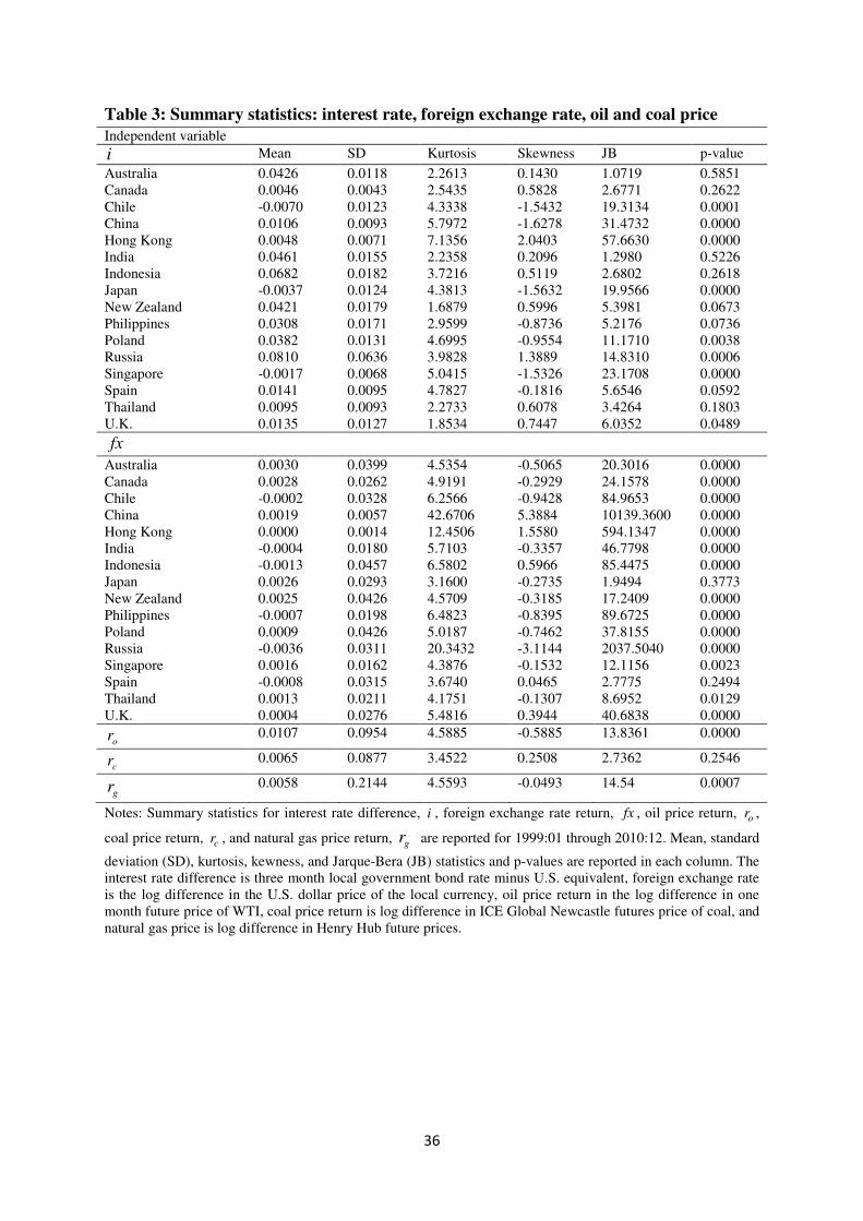
Table 3 presents summary statistics of foreign exchange and interest rate differences

by country. Over the 1999-2010 period most of countries have higher short-term interest rate

than U.S. The interest rate difference between the local three-month government bond rate

and that for the U.S. is positive for thirteen countries and negative for Japan, Chile and

Singapore. Over 1999-2010, on average, ten currencies appreciated against the U.S. dollar

and six currencies did not. The standard deviation of foreign exchange rate change against the

U.S. dollar is highest for Indonesia, New Zealand and Poland. Kurtosis of foreign exchange

rate returns is more than three and these returns tend to be negatively skewed. The null

hypothesis of Jarque-Bera tests is rejected implying the returns are not normally distributed.

Summary statistics on oil price returns, coal returns and natural gas price returns are

provided at the bottom of Table 3. Oil price returns and coal price returns have positive mean

9

monthly values. Oil price returns are higher than the coal price returns by factor of about

65%. The standard deviation of oil price returns is also higher than that for coal price returns,

but in the monthly data only by a proportion of about 8.8%. This is consistent with the

finding by Pindyke (1999) that over 125 years of price data oil price was more volatile than

coal price. Regnier (2007) notes that volatility and relative volatility of energy prices can

vary over time depending on regulation, market structure, output elasticity and

substitutability in use. Oil returns are negatively skewed and coal returns are positively

skewed. The Jarque-Bera statistics imply that the null hypothesis that oil price returns are

normally distributed is rejected and that the null hypothesis that coal price returns are

normally distributed is not rejected.

Figure 1 displays coal price and oil price from January 1999 to December 2010. The

energy prices do tend to track one another. Figure 1 reveals that there were upward jumps in

prices from 2007 that continued until the Global financial crisis in September-October, 2008.

During the Global financial crisis there were significant drops in oil and coal prices, with the

drop in oil price occurring earlier than the drop in coal price. In the monthly data, oil price

peeked in July 2008 and coal price peeked in September 2008. Prices started recovering in

late 2009, with the recovery in oil price starting earlier than that in coal prices. Movement in

prices between oil and coal will diverge depending on circumstances that impact relative

inventories of coal and oil available to users. Coal price achieved a local peak in July 2004.

During this period power generation companies experience low coal reserves during severe

power shortages in China, the world’s largest producer of coal. Figure 2 displays coal price

return and oil price return from January 1999 to December 2010. Both the oil and coal price

return series exhibit large swings in the monthly data. The Figure 2 suggests that the timing

of these swings may not be that strongly related.

10

The correlation matrix of variables is provided in Table 4. Coal and oil price returns

have a positive co-movement and correlation coefficient of 0.22. The highest correlation

(0.66) is between local stock market excess return and global stock market excess return.

These two variables will not appear simultaneously in the same regression. The foreign

exchange rate return and local stock market return have correlation coefficient of 0.42, with

the implication that there is positive co-movement between a strengthening currency and

increasing local stock market returns. The pair wise correlations among the other variables

are not high in absolute value. Coal and oil price returns have a positive co-movement and

correlation coefficient of 0.22. Coal price return volatility has correlations of 0.01, -0.19 and -

0.31, with coal price returns, oil price returns and oil price return volatility, respectively. Oil

price return volatility has correlations of -0.04 and 0.18 with coal price returns and oil price

returns, respectively. It is likely that overall, multicollinearity is not a problem in estimating

linear regression models with these variables.

3. Arbitrage pricing regressions and oil price variables

3.1. The basic regression

In the basic model the risk factors are taken to be market return, the foreign exchange

return, an interest rate differential, and coal and oil price returns. The basic model is given by

, , , , , , ,i t wm wm t in i t fx i t c c o o t i tr r i fx r rα β β β β β µ= + + + + + +

1, 2,.... ,i l= (2)

where ,i tr represents the excess return of the coal sector of country i at time t,

,wm tr represents

the global market excess return at time t, ,i ti is the interest rate difference between the short-

term interest rate of country i and 3-month U.S. T-bill rate, tifx , is the foreign exchange

return (log difference in U.S. dollar price local currency) of country i , ,c tr is the coal price

return, ,o tr is the oil price return, α is a constant, and

,i tµ is an error term. An alternative to

11

the basic model will substitute local market excess return (,lm tr ) in equation (2) for global

market excess return.

If the estimated coefficient of ,o tr ,

oβ , is statistically significant in equation (2), then

oil price return provides information for coal stock returns beyond that conveyed by coal

price return. Rejection of the null hypothesis o cβ β<

indicates that oil price return is at least

as important in explaining coal sector returns as is coal price returns.

In equation (2), the returns ,i tr ,

,wm tr , ,lm tr ,

,c tr and ,o tr are expressed as U.S. dollar

returns. A test of the null hypothesis that the exchange rate has no influence on local currency

returns in the coal sector other than through the impacts on local currency denominated

market (either global or local), coal and oil returns is provided by testing Ho:

1wm fx c oβ β β β+ + + = (or Ho: 1lm fx c oβ β β β+ + + = ). If the null hypothesis is not rejected,

upon substitution, equation (2) becomes (the superscript L indicates local currency-

denominated returns):

, , , , , , ,L L L L

i t wm wm t in in t c c t o o t i tr r i r rα β β β β µ= + + + + +

1, 2,.... ,i l= (2’)

with the foreign exchange term removed, since , , ,

L

z t z t i tr r fx≡ − , , , , ,z i wm lm c o= .

3.2. Energy price volatility

The volatility of energy price returns has also been considered as an influence on

stock returns. Bernanke (1983) and Pindyck (1991) contend that uncertainty is detrimental to

economic activity and that oil price return volatility has a negative impact on economic

activity and the stock market. Veronesi (1999) presents a theoretical model linking economic

uncertainty and stock market volatility, arguing that during periods of high uncertainty

investors are more sensitive to news and that this increases asset price volatility. Sadorsky

(1999) identifies oil price shocks and oil price volatility as playing an important role in

explaining U.S. real stock returns. Park and Ratti (2008) state that increased volatility in

12

energy prices causes greater uncertainty about product demand and future returns on

investment, and affects the present value of future dividends.

Oil and coal return volatility is measured as the moving average of the squared

residuals obtained from AR(1) regressions for oil and coal price returns. The AR(1)

regression equations are given by:

, , 1 ,o t o o o t o tr c rϕ ε−= + + (3a)

, , 1 ,c t c c c t c tr c rϕ ε−= + +

(3b)

The measure of oil and coal price return volatility is given by the residuals from equations

(3a) and (3b), ,

ˆo tε

and

,ˆ

c tε :

( )0.5

1 2

, ,

0

ˆ1m

k t k t j

j

mσ ε−

−=

= +

∑ , ,k o c= (4)

with t = 0 ..., n-m-1 and m=4. Volatility in oil and coal price returns is based on innovations

that are not explained by past oil and coal price changes. Volatility has been measured in this

way by Gallant and Tauchen (1998).

An arbitrage pricing model that captures the effects of energy price volatility is given

by:

, , , , , , , ,i t wm wm t in i t fx i t c c o o t coalvol c t oilvol o t i tr r i fx r rα β β β β β β σ β σ µ= + + + + + + + + , 1, 2,.... ,i l= (5)

where volatility in coal and oil price returns is given by ,c tσ and ,o tσ , respectively.

3.3. Asymmetric effects of oil and coal price returns

Asymmetry in the effect of energy prices on coal sectors will also be examined. In the

literature oil price increases have been found to have a greater influence in absolute value on

the macroeconomic aggregates than have oil price decreases. This asymmetric effect has been

documented by Mork (1989), Hooker (1996; 2002), Hamilton and Herrera (1999) and Balke

et al. (2002), amongst others for the U.S., by Lee et al. (2001) and Zhang (2008) for Japan,

13

by Huang et al. (2005) for Canada, Japan and the U.S., by Cologni and Manera (2000) for the

G-7, by Cunado and Garcia (2003) for most European countries, and by Lardic and Mignon

(2008) for G7 and Europe and Euro area countries. It has long been noted that counter-

inflationary monetary policy responses to oil price increases can lead to the appearance of

asymmetric effects of oil price increases and decreases.

Hamilton (1988) argues that change in energy price creates sectoral imbalance, which

in the presence of imperfect labour mobility results in short-run loss of output, which is

reinforced by oil price increases and mitigated by oil price decreases. Asymmetric effects of

oil price increases and decreases grounded in sectoral reallocations is reported as a basic

finding by Jones et al. (2004) in their survey of the literature on the effects of oil price

shocks. Edelstein and Kilian (2007) contend that a finding of asymmetry is due to not

modelling the effects of tax reform on fixed investment and failure to disaggregate

investment into energy and non-energy related investment.

Asymmetric effects of oil price on real activity have also been grounded in the effects

of uncertainty on real activity. Ferderer (1996) reports that oil price changes affect oil price

volatility and that the latter has a negative effect on the economy. Elder and Serletis (2010)

find that controlling for oil price uncertainty reinforces the negative response in real output to

higher oil prices and ameliorates the gain in real output in response to lower oil prices.

Rahman and Serletis (2011) argue that negative and positive oil price shocks differ in their

impact on the volatility of oil price changes. Asymmetry in the effect of oil price on real

activity may also be due to asymmetric effects of crude oil price on energy prices at the retail

level. Kaufmann and Laskowski (2005) argue an asymmetry arises between crude oil price

and gasoline price due to refinery utilization and optimal inventory behaviour, and between

crude oil price home heating oil due customer contracts.

14

Nandha and Faff (2008) do not observe an asymmetric effect of oil price returns on

global sector returns. Park and Ratti (2008) find evidence of asymmetric effects of oil price

increases and decreases on real stock returns for the U.S. and for Norway, but not for oil

importing European countries. Arouri (2011) notes that asymmetric effects of oil price

increases and decreases on sectoral stock prices may arise because sectors differ with regard

to energy intensity of production, the use of energy associated with the final product, and the

degree of imperfect competition and ability to pass on cost increases to consumers.

To test the asymmetric effect of oil price change on coal sector returns, positive

change in energy price, ,

pos

k tr ( ,k o c= ), is differentiated from negative changes in energy

price, ,

neg

k tr ( ,k o c= ), as follows:

, 1max{0, ln( ) ln( )}pos

k t t tr k k −= − ,k o c= (6a)

, 1min{0, ln( ) ln( )}neg

k t t tr k k −= − ,k o c= (6b)

where tc is the monthly logarithmic change in ICE Global Newcastle futures coal price in US

dollar per metric tonne, to is the 1-month future price of a barrel of WTI (in U.S. dollars).

The model is augmented by incorporating these asymmetric measures of oil and coal

returns into the following equations:

, , , , , , ,

p pos n neg

i t wm wm t i i t fx i t c c o o t o o t i tr r i fx r r r uα β β β β β β= + + + + + + + (7)

ti

neg

tc

n

c

pos

tc

p

cootifxtiintwmwmti rrrfxirr ,,,,,,, µββββββα +++++++= (8)

Examination of asymmetric effect of coal (oil) price return on coal company stock

will be based on inclusion of the oil (coal) price return in the regression equation. Increases

and decreases in coal and in oil price should have positive coefficients in equations (7) and

(8). The effect of oil price as a signal for overall energy demand could lead to asymmetric

effects if rising oil price (and rising demand for energy) is expected to lead to greater use of

coal in the future than falling oil price (and falling demand for energy) for energy is thought

15

to lead to decreased use of coal in future. A change in oil price as change in price of

substitute for coal could also be asymmetric in effect, depending on the circumstances in

which it is possible for substitution between these primary sources of energy. Equation (7)

provides a test of the null hypothesis (Ho:pos neg

k kβ β= , ,k o c= ) that there is no difference

between positive and negative shocks of either oil and coal price returns.

3.4. Net oil price and net coal price changes

The effect of large sustained increases in coal and oil prices will also be investigated.

Net oil price increase, introduced by Hamilton (1996), is designed to capture how unsettling

an unusually large increase in the price of oil is likely to be for the spending decisions of

consumers and firms. It is argued by Lee et al. (1995) that oil price increases at a time when

oil prices have been relatively stable is likely to have a larger effect than an increase in oil

prices at a time when oil prices have been relatively volatile.

Following Hamilton (1996), net energy price increase, tnkpi ( ,k o c= ), and by

analogy net energy price decrease, tnkpd ( ,k o c= ), are defined as:

( )( )1 12max{0, ln( ) ln max ,........, }t t t t

nkpi k k k− −= − ( ,k o c= ) (9a)

( )( )1 12min{0, ln( ) ln min ,........, }t t t t

nkpd k k k− −= − ( ,k o c= ) (9b)

Net energy price increase (decrease) measures the amount by which log price of

energy exceeds (is below) its maximum (minimum) over the last twelve months. Coal sector

returns might react more to a coal or an oil price return that takes coal or oil price to a twelve

month high than a coal or an oil price increase that does not. These nonlinear transformations

have been used in analysis of the macroeconomic effects of oil prices (see for instance

Bernanke et al., 1997; Lee and Ni, 2002). Kilian (2008) argues that net oil price increase may

be a good measure of the exogenous component of oil price movement. Figure 3 displays the

net oil price increase variable ( nopi ). Net oil price increase takes on positive values in 2000,

16

2004-5 and 2007-8. Figure 4 displays the net coal price increase variable ( ncpi ). Net coal

price increase takes on larger positive values in 2004 and 2007.

A Model that captures the effects of net coal price increase and decrease and of net oil

price increase and decrease is given by:

, , , , , , ,nkpi nkpd

i t wm wm t in i t fx i t c c o o t o t o t i tr r i fx r r nkpi nkpdα β β β β β β β µ= + + + + + + + + ,k o c= (10)

Estimation of equation (10) provides a test of the hypothesis (Ho: 0nopi

oβ = ) that coal sector

returns react more to an oil price return that takes oil price to a twelve month high than an oil

price increase that does not. A test of the hypothesis that an oil price decline that takes oil

price below the level seen in the previous twelve months has a differential impact on coal

sector returns compared to an oil price decline that does not is provided by Ho: 0nopd

oβ = .

Also, estimation of equation of (10) provides a test of the null hypothesis ( nopd

o

nopi

o ββ = ) that

coal sector returns do not react differently between oil price returns that take oil price to

either a twelve month high or to a twelve month low. A similar examination can be made of

the hypothesis that coal sector returns react differently to coal price returns that take coal

price to a twelve month high than to coal price returns that take coal price below the level

seen in the previous twelve months.

4. Results

The international factor model equations for excess coal sector returns in section 3

are estimated as a panel. We estimate fixed effects using ordinary least squares and random

effects panels using generalized least squares (GLS) method. Fixed effects method is

advantageous if the country effects are correlated with the explanatory variables. Hausman

test results are obtained for all specifications with the null hypothesis of no correlation (the

random effects model is the null hypothesis). The test results for the equations show that the

null hypothesis cannot be rejected in all cases. In what follows only results for random effect

17

panels are reported.2 Data on coal sector, global and local market returns are winsorized at

the 1st percentile and 99

th percentile to deal with the outliers. It turns out that this procedure

does not greatly affect results.

In Table 5, two sets of results are reported: in panel A with global stock market index

return as market return; and in panel B with local benchmark stock index return as the market

return. In each panel 6 regression equations are reported. Market excess return, the interest

rate difference and foreign exchange return appear in all equations and coal and oil excess

returns and volatilities appear in different combinations in equations in order to determine

whether results obtained from estimating equations (2) and (5) in the text are robust.

Estimates of equations (2) and (5) appear in columns 4 and 6, respectively, in Table 5. Since

equation (5) is the most comprehensive of the equations estimated, the results in column 6 of

Table 5 will be given most attention. In all regressions in Table 5 market excess return, the

interest rate difference, foreign exchange return, coal price return, and oil return and oil

return volatility are statistically significant. The Wald test statistic for panel data indicates the

models are statistically significant.

In Table 5, the coefficient of global market index return,wmβ , in panel A and the

coefficient of global market index return,lwβ , in panel B are statistically different from zero at

1% level of confidence. All these parameter estimates are less than 1, significantly so for the

estimates of lwβ in columns (1) through (6) and for the estimates of

wmβ in columns (5) and

(6).3 These results suggest that the equity of the coal sector is less volatile than market

returns. Since in each column, the estimate of lwβ is less than

wmβ it appears that coal sector

returns are more sensitive to systematic risk in the global economy than to systematic risk in

the local economy. In addition, the R2

results for regressions for coal sector returns are

2 The fixed effect results and Hausman test results are available upon request.

3 For example, a one-tailed test that the market beta in panel A in column (6) is less than 1 has a t-statistic of

1.982 and a one-tailed test that the market beta in panel B in column (6) is less than 1 has a t-statistic of 4.576,

and the 5% and 1% critical values for one-tailed tests are 1.658 and 2.358, respectively.

18

somewhat higher when market risk is measured by global market return than by local market

return. It will be observed later that this pattern is most pronounced for coal returns in

emerging economies. Thus, it is concluded that coal sector returns are strongly influenced by

global market developments.4

The estimate of the coefficient of foreign exchange rate risk (a rise indicates an

appreciation of the local currency) is positive and statistically significant at the 1% level in all

regressions in Table 5. The appreciation of the local currency against the U.S. dollar

generates positive coal industry returns, results similar to the findings of Sadorsky (2001),

Boyer and Filion (2007), and Ramos and Veiga (2011) for oil and gas sector returns. The

result is consistent with a money demand model in which domestic currency and stock

returns move together over the cycle (Solnik and McLeavey (2009)). Real growth is

associated with increased stock returns and a rise in money demand that causes a rise in the

value of the domestic currency. A test of the null hypothesis that the exchange rate has no

influence on local currency returns in the coal sector other than through the impacts on local

currency denominated market, coal and oil returns (Ho: 1wm fx c oβ β β β+ + + = ) is not rejected

in columns 4 and 6 of Table 5. Thus, the hypothesis that the true relationship determining

local currency returns in the coal sector is given by equation (2’) is not rejected.5

The estimate of the coefficient of the interest rate difference is negative and mostly

statistically significant in Table 5. Tighter liquidity in a country tends to lower returns in the

coal sector. This is consistent with monetary tightening signalling macroeconomic slowdown

with a dampening future demand for energy. In addition, the coal sector is capital intensive

4 These results for coal sector returns are different from results found for oil and gas companies by Ferson and

Harvey (1994) and Ramos and Veiga (2011). They find that if anything, local market return has a stronger

influence on oil and gas sector returns than world market portfolio return. 5 Faff and Brailsford (1999) report a similar outcome for most Australian sectors including the oil and gas

sector, in that in an equation with all returns expressed in local currency the exchange is not statistically

significant.

19

and higher interest rates increase the cost of carrying debt and of financing investment with

negative implications for coal sector returns.

4.1. Coal and oil price returns

The coal price return is statistically significant at 1% level in determining excess

return in the coal sector in all the regressions in Table 5. A 1% increase in coal price return

raises the coal company returns by between 0.270% and 0.291%. The results are consistent

with and analogous to findings that oil price returns are positively associated with the returns

of oil and gas companies. Sadorsky (2001) and Boyer and Filion (2007), for example, find

that a 1% increase in oil price raises the return of Canadian oil and gas companies by about

0.300%. Mohanty and Nandha (2011) report that a 1% increase in oil price raises return in the

U.S. oil and gas sector by between 0.207% and 0.378% depending on time period. Ramos

and Viega (2011) report a smaller effect (about 0.144%) of oil price returns on returns in the

oil and gas sector worldwide.

In the coal sector results in Table 5 oil price return is statistically significant at 1%

level in determining excess return in the coal sector in all regressions. The magnitude of the

effect of oil price return on coal sector return is sensitive to whether or not a coal price return

variable appears in the regression. However, in regressions including oil and coal price

returns, a 1% increase in oil price return raises coal sector returns by between 0.120% and

0.132%. Oil prices may have a sizeable impact on coal sector stock when coal price returns

are included in the regression, because among energy commodities, crude oil gets more news

coverage and attention by market participants and researchers. For example, Gogineni (2008)

reports that during the years 2005 and 2006, oil prices figured in the headlines of The Wall

Street Journal on 204 days, and a majority of the accompanying articles attributed stock price

movements the previous day to oil price changes.

20

Participants in the energy markets may perceive oil price as being determined globally

and as reflecting future global demand for energy overall more efficiently than does coal

price. For this reason crude oil price developments have influence on coal sector stocks.

Bachmeier and Griffin (2006) conclude from examination of five crude oils that the world oil

market is a single integrated economic market, but the coal market is not, and that a primary

global energy market overall is only existent in the long run. Humphreys and Welham (2000)

observe that the coal industry by the 1990s had started to emerge as a global industry.

Ekawan and Duchêne (2006) observe that the spot market had become much more important

over time for trade in coal in the Atlantic region, with the fraction of spot market trade rising

from 14% in 1983 to 80% of the total in 2003. It is noted by Ekawan et al. (2006) that spot

markets have also become much more important for trade in coal in the Pacific region. Warell

(2006) find that the market is globally integrated for coal. Li (2010) provides a review of the

growth in an international market in steam coal and concludes that progress toward a fully

developed spot market is well advanced. Li et al. (2010) find a stable long run cointegrating

relationship between price series for coal in Europe and Japan that is supportive of a globally

integrated market for coal.

In results not reported it is found that oil price risk orthogonal to coal price risk,

obtained from the residuals of a regression of oil price return on coal price return, also

significantly influences coal stock returns. The results imply that oil price return increases not

reflected in coal price returns also have a positive effect on coal company stock returns.

4.2. Coal and oil price return volatilities

In Table 5 the result from estimating equation (5), in which the standard deviations of

coal and oil price return volatilities appear, is reported in column 6. The coefficient of coal

return volatility in column 6 in Table 5 is negative but is not statistically significant when

21

market risk factor is measured global stock market returns and is only statistically significant

at the 10% level when market risk factor is measured by local stock market returns. Oil price

return and volatility also appear in this equation. The coefficient of coal return volatility in

column 2 in Table 5 is negative when oil price return and volatility do not appear in the

regression. It is interesting that Ramos and Veiga (2011) find that increased oil price return

volatility is associated with an increase in oil and gas sector returns. Thus, the response of

coal sector returns to coal price return volatility contrasts with results observed for the

response of oil and gas sector returns to oil price return volatility (when sector return is

regressed solely on own product price return volatility).

Oil price return volatility has a negative statistically significant effect at the 1% level

on coal sector returns. This return holds when market risk factor is measured global stock

market returns (panel A) and by local stock market returns (panel B). An increase in oil price

return volatility by its mean value decreases coal sector returns by 13.04% (9.93%) when

market risk factor is measured by global stock market returns (local stock market returns).6

This result is in line with that reported by Park and Ratti (2008) and Sadorsky (1999) that

increased volatility in oil price reduces stock price returns measured by a general index.

4.3. Different groups of countries

This section examines whether results are sensitive to the groups of countries

considered. Issues that arise concern differing degrees of integration into world market by

sectors in emerging countries and the differing effect of coal and oil price indices on coal

sector returns in different markets.

4.3.1. Developed countries vs. Emerging countries

6 The mean of oil (coal) price return volatility defined in equation (4) is 0.0867 (0.0796). The product of the

coefficient of oil price return volatility in Table 5, column 6, panel A (B), -1.5041 (-1.1458), and 0.0867 yields -

0.1304 (-0.0993).

22

The issue of whether risk factors in coal sector returns differ between developed and

emerging countries is investigated in this section. Emerging markets may not be fully

integrated into the global economy and this may give rise to differences in the effect of the

risk factors on coal sector returns. Carrieri and Majerbi (2006) report that returns in emerging

markets are affected more by local than by global risk factors. Basher and Sadorsky (2006)

find that stock markets of emerging countries are more exposed to oil price risk factor than

stock markets in developed countries. Table 6 presents results of the GLS panel estimation of

coal sector returns in developed countries in column 1 and in emerging countries in column 2.

Developed and emerging markets are identified according to MSCI classification.7

The goodness of fit of the regressions measured by R2 is better for explaining coal

sector returns in developed markets than in emerging markets, reflecting the greater volatility

in general in returns in the emerging markets. In column 1 for developed markets it doesn’t

much matter whether the market risk factor is measured by a global market index or a local

market index, since developed markets are well integrated into the global market. In column

2 for emerging markets coal sector returns are more exposed to global market systematic risk

than to local market systematic risk. However, coal sector returns in emerging markets are

less exposed to global market systematic risk than are coal sector returns in developed

markets. In the regression equations disaggregated by developed and emerging markets,

although the estimated coefficient of the interest rate difference is negative it is no longer

statistically significant in most regressions. Foreign exchange rate risk is statistically

significant at the 1% level for both the developed and emerging markets in regressions with

global market risk and less so in regressions with local market risk.

The coefficients of coal price return and oil price return are positive and statistically

significant in regressions for coal sector returns in both developed and emerging markets. In

7 Developed countries are Australia, Canada, Hong Kong, Japan, New Zealand, Singapore, Spain, U.K. and U.S.

Emerging countries are Chile, China, India, Indonesia, Poland, Philippines, Russia and Thailand. Ramos and

Veiga (2011) use MSCI classification in their study of risk factors in oil and gas industry returns.

23

Panel A with global market risk, the exposure of coal sector return to coal price return is

greater than that to oil price return for both developed and emerging markets. This result is

unchanged for the developed countries but is changed for emerging counties when local

market risk is substituted for global market risk.

4.3.2. Asia-Pacific and Pacific countries

Robustness of results will now be examined for Asia-Pacific and Pacific countries.

This will provide a check of robustness of results across regions where the ICE Global

Newcastle futures contract coal price is the leading price benchmark for seaborne thermal

coal. Four sub-groups are considered. Asia-Pacific1 countries are Australia, Canada, Chile,

China, Hong Kong, India, Indonesia, Japan, New Zealand, Philippines, Russia, Singapore,

Thailand and U.S. Pacific1 countries are Australia, Canada, Chile, China, Hong Kong,

Indonesia, Japan, New Zealand, Philippines and Singapore. Asia-Pacific2 countries are Asia-

Pacific1 countries minus Russia and the U.S. Pacific

2 countries are Pacific

1 countries minus

China and Hong Kong.

Estimates of regression equation (2) are reported in columns 3 through 6 for these

four groups of countries. It is found that coal sector returns in the groups of Asia-Pacific and

Pacific markets are exposed to global market systematic risk, foreign exchange and interest

rate risk, and coal price and oil price return. Coal and oil price return have statistically

significant effects on coal sector returns across different groups of country. A test of the null

hypothesis that the exchange rate has no influence on local currency returns in the coal sector

other than through the impacts on local currency denominated market, coal and oil returns is

not rejected in columns 3 through 6 in Table 6 for any of the country groups.

4.4. Asymmetric effects of coal price and oil price changes

Test results for an asymmetric effect of oil and coal price changes on coal sector

returns are reported in Table 7. Estimates of equations (7) and (8) for positive and negative

24

oil and coal price returns are reported in columns 1 and 2, respectively, and estimates of

equation (10) for net oil and coal price returns are reported in columns 3 and 4, respectively.

Positive change in coal price, ,

pos

c tr , is statistically significant at the 1% level of confidence in

column (1) and positive change in oil price, ,

pos

o tr , is statistically significant at the 1% level of

confidence in column (2). The coefficients of the negative oil and price changes are also

statistically significant in columns (1) and (2), but are smaller in magnitude than the

coefficients of the positive oil and price changes. The null hypothesis that positive and

negative coal price shocks have the same coefficient is rejected at the 1% level of confidence

and the null hypothesis that positive and negative oil price shocks have the same coefficient

is rejected at the 10% level of confidence. These results suggest that coal (oil) price increases

have a larger positive impact on coal sector returns than coal (oil) price decreases have on

decreases in coal sector return.

In column 3 of Table 8 the coefficient of net coal price increase is statistically

significant at 5% level. The coefficient of net coal price decrease is negative in column 3. A

Chi-square test of the null hypothesis ncpi ncpd

c cβ β= is rejected at the 1% level. In column 4 of

Table 7 the coefficient of net oil price increase is statistically significant at the 1% level of

confidence. A positive value for net oil price indicates that oil price is trading at a higher

price than that observed over the previous twelve months. Coal sector returns react more to

an oil price return that takes oil price to a twelve month high than an oil price increase that

does not. The coefficient of net oil price decrease is statistically significant at the 10% level.

The coefficient of nopi is larger than that of nopd . A Chi-square test of the null hypothesis

nopd

o

nopi

o ββ = is rejected at the 1% level. Thus, oil price declines that take oil price below the

level seen in the previous twelve months does have a larger impact than a regular oil price

25

decline (at least at the 10% level of confidence) but this differential effect is not as marked as

that for oil prices breaking higher levels.

The pass-through effect of coal and of oil price returns for coal sector returns are

similar to those observed by Ramos and Veiga (2011) for oil price returns on oil and gas

sector returns, in that coal and oil price increases have larger effects than oil price decreases.

In column 5 of Table 7 net oil and coal price increases and decreases appear together. The

asymmetry between positive and negative net oil and coal price changes is again confirmed.

Thus, it can be said that the asymmetry effect is observed in the coal sector returns.

4.5. Natural gas price returns

We augment this study by evaluating the effect of natural gas price returns on the coal

sector returns. This allows examination of whether controlling for natural gas returns renders

the influence of oil price returns on coal sector returns insignificant. Coal and natural gas are

energy sources used for electricity and heating production and not considering the influence

of gas price returns might bias results. In our work we use the log difference of monthly

Henry Hub future price of natural gas- the leading price in natural gas market (a U.S. dollar

index). From Table 2 it can be seen that gas price returns are slightly less than coal price

returns over 1990:01 to 2010:12. The standard deviation of gas price returns is over twice that

for either coal price returns or oil price returns. As for coal price returns (and not for oil price

returns) the Jarque-Bera statistic implies that the null hypothesis that gas price returns are

normally distributed is not rejected. In Table 4 gas and coal price returns have a positive co-

movement and correlation coefficient of 0.07, and gas and oil price returns have a positive

co-movement and correlation coefficient of 0.15. The values of these correlations indicate

that inclusion of oil, coal and gas returns in the same regression do not raise multicollinearity

issues.

26

We use the following model to evaluate the effect of gas price returns on coal sector

returns:

, , , , , , ,i t wm wm t in i t fx i t c c o o t g g i tr r i fx r r rα β β β β β β µ= + + + + + + + (11)

where gr is gas price return. Results from estimating equation (11) are reported in Table 8.

When gas price return is the only energy price appearing in the regression equation, the

coefficient of natural gas price is significant at 10% level (column 1). However, when oil

price return appears in the regression equation the coefficient of gr is not statistically

significant (in column 2 and 3 of Table 8). Both coal and oil price returns are statistically

significant in the presence a gas price return variable, with coefficients of 0.11 and 0.24,

respectively in column 3 of Table 8. The null hypothesis that the effect of oil price return on

coal sector return is less than that of coal price return on coal sector return (Ho: o cβ β< ) is

rejected at the 1% level. Thus, the result that oil price return has a larger impact on coal

sector return than does coal price return is not affected by inclusion of gas price return in the

regression equation.

5. Conclusion

In this paper we examine panel data on coal sector stock price indices available at

country level and evaluate risk factors significant in determining return in the coal sector. The

paper studies the effect of energy shocks on coal sector stock returns and supplements

research evaluating the effect of oil prices on the stock price of oil and gas companies. A 1%

increase in coal price return raises the coal company returns by between 0.27% and 0.29%.

This result is robust across developed, emerging and differing groups of Asia-Pacific and

Pacific countries. The results are consistent with analogous findings that a 1% increase in oil

price raises the return of oil and gas companies by between 0.14% and 0.38% depending on

country and time period studied.

27

The paper finds that oil prices have a significant impact on coal sector returns even in

the presence of coal price returns. A 1% increase in coal price raises coal sector returns by

about 0.12%. This result may follow because news about energy commodities focuses

primarily on oil price. Research supports the view that the market for crude oil is an

international market, whereas the market for coal is only more recently emerging as a global

market. Participants in the market may perceive oil price as serving as the bench mark for

future global demand for energy overall. For this reason crude oil price developments have

influence on coal sector stocks. Natural gas prices do not influence coal sector returns in the

presence of coal price returns.

Coal sector returns react more to an coal price return that takes coal price to a twelve

month high than an coal price increase that does not. The coal sector responds more to a

positive coal price change than to negative coal price change. It should be noted that

estimation of asymmetric effects of coal price change does not erode the statistical

significance of oil price change in affecting on coal sector returns. An asymmetry in the

effect of oil prices on coal sector returns is also observed. Coal sector returns react more to an

oil price increase than to an oil price decrease and more to an oil price return that takes oil

price to a twelve month high than an oil price increase that does not. Increased volatility in oil

price return significantly reduces coal sector return. Increased coal price volatility does not

significantly affect coal sector return.

Market return, interest rate premium, foreign exchange rate risk, and coal price

returns are statistically significant in determining the excess coal sector stock returns.

Currency depreciation has a negative impact on the return of coal companies, a result similar

to that found by comparable country studies for oil and gas companies. The exchange rate

does not significantly influence local currency returns in the coal sector other than through

the impacts on local currency denominated market, coal and oil returns. Understanding the

28

variables that affect the behaviour of stock prices of coal companies is of importance to

market participants and to policy makers for developing efficient hedging policies for dealing

with oil and energy price shocks.

29

References

Apergis, N., Miller, S.M., 2009. Do structural oil-market shocks affect stock prices? Energy

Economics 31-4, 569-575.

Arouri, M.E.H., 2011. Does crude oil move stock markets in Europe? A sector

investigation. Economic Modelling 28, 1716-1725.

Arouri, M.E.H., Jouini, J., Nguyen, D.K., 2011. Volatility spillovers between oil prices and

stock sector returns: Implications for portfolio management. Journal of International

Money and Finance, 30, 1387-1405.

Bachmeier, L., Griffin, J., 2006. Testing for market integration: crude oil, coal, and natural

gas. The Energy Journal 27, 55-71.

Balke, N.S., Stephen, P.A., Yucel, M.K., 2002. Oil price shocks and the U.S. economy:

where does the asymmetry originate. The Energy Journal 23, 27-52.

Basher, S., Sadorsky, P., 2006. Oil price risk and emerging stock markets. Global Finance

Journal17, 224-251.

Bernanke, B.S., 1983. Irreversibility, uncertainty, and cyclical investment. Quarterly Journal

of Economics 98, 115-134.

Bernanke, B.S., Gertler, M., Watson, M., 1997. Systematic monetary policy and the effects of

oil price shocks. Brookings Papers on Economic Activity1, 91-157.

Boyer, M.M. Filion, D., 2007. Common and fundamental factors in stock returns of Canadian

oil and gas companies. Energy Economics 29, 428-453.

Brown, S., Yücel, M., 2008. What drives natural gas prices? The Energy Journal 29, 45-60.

Carrieri, F. Majerbi, B., 2006. The pricing of exchange risk in emerging stock Markets.

Journal of International Business Studies 37, 372-391.

Chen, N.F., Roll, R. Ross, S., 1986. Economic forces and the stock market. Journal of

Business 59, 383-403.

Ciner, C., 2001. Energy shocks and financial markets: nonlinear linkages. Studies in Non-

Linear Dynamics and Econometrics 5, 203-12.

Cologni, A., Manera, M., 2009. The asymmetric effects of oil shocks on output growth: a

Markov-switching analysis for the G-7 countries. Economic Modelling 26, 1-29.

Cunado, J., Garcia, F., 2003. Oil prices, economic activity and inflation: evidence for some

Asian countries. The Quarterly Review of Economics and Finance 45, 65-83.

Dayanandan, A., Donker, H., 2011. Oil prices and accounting profits of oil and gas

companies. International Review of Financial Analysis 20, 252-257.

30

Driesprong, G., Jacobsen, B., Matt, B., 2008. Striking oil: another puzzle. Journal of

Financial Economics 2, 307-327.

Edelstein, P., Kilian, L., 2007. Retail energy prices and consumer expenditures. University of

Michigan.

Ekawan, R., Duchêne, M., 2006. The evolution of hard coal trade in the Atlantic market.

Energy Policy, 34-13, 1487-1498.

Ekawana, R., Duchêne, M., Goetz, D., 2006. The evolution of hard coal trade in the Pacific

market. Energy Policy 34, 1853-1866.

Elder, J. Serletis, A., 2010. Oil price uncertainty. Journal of Money Credit and Banking 42,

1137-1159.

El-Sharif, I., Brown, D., Burton, B., Nixon, B. Russell, A., 2005. Evidence on the nature and

extent of the relationship between oil prices and equity values in UK. Energy

Economics 27, 819-830.

Faff, R.W. Braislsford, T.J., 1999. Oil price risk and the Australian stock market. Journal of

Energy and Finance Development 4, 69-87.

Ferderer, J.P., 2006. Oil price volatility and the macroeconomy. Journal of Macroeconomics

18, 1-26.

Ferson, W., Harvey, C., 1994. Sources of risk and expected returns in global equity markets.

Journal of Banking & Finance 21, 1625-1665.

Gallant, A. Tauchen, G., 1998. Reprojecting partially observed systems with application

to interest rate diffusions. Journal of the American Statistical Association 93, 10-24.

Gogineni, S., 2008. The stock market reaction to oil price changes. Working paper,

University of Oklahoma Norman, no. 73019-0450.

Hamilton, J.D., 1988. A neoclassical model of unemployment and the business cycle. Journal

of Political Economy 96, 593-617.

Hamilton, J.D., 996. This is What Happened to the Oil Price-Macroeconomy

Relationship. Journal of Monetary Economics 38, 215-220.

Hamilton, J.D., Herrera, M.A., 2002. Oil shocks and aggregate macroeconomic

behaviour. Journal of Money, Credit and Banking 36, 265-286.

Hooker, M.A., 1996. What happened to the oil price-macroeconomy relationship? Journal of

Monetary Economics 38, 195-213.

Hooker, M.A., 2002. Are oil shocks inflationary? Asymmetric and nonlinear specifications

versus changes in regime. Journal of Money, Credit and Banking 34, 540-561.

31

Huang, B.N., M.J. Hwang, Peng, H.P., 2005. The asymmetry of the impact of oil price

shocks on economic activities: An application of the multivariate threshold model.

Energy Economics 27, 455-476.

Huang, R.D., Masulis, R.W., 1996. Energy shocks and financial markets, Journal of Futures

Markets 16, 1-27.

Humphreys, D., Welham, K., 2000. The restructuring of the international coal

industry. International Journal of Global Energy Issues 13, 333-355.

Ibrahim, O., 2009. Natural gas markets: How sensitive to crude oil price changes? Munich

Personal RePEc Archive, <http://mpra.ub.uni-muenchen.de/14937/>.

Jones, C.M., Kaul, G., 1996. Oil and the stock markets. Journal of Finance 51, 463-491.

Jones, D.W., Leiby, P.N., Paik, I.K., 2004. Oil price shocks and the macroeconomy: what has

been learned since 1996? The Energy Journal 25, 1-32.

Kilian, L., 2008. Exogenous oil supply shocks: how big are they and how much do they

matter for the US economy? Review of Economics and Statistics 49, 823-852.

Koller, T., Goedhart, M., Wessels, D., 2010. Valuation: Measuring and managing the value

of the companies. 4th edn, John Wiley & Sons, New Jersey.

Lardic, S., Mignon, V., 2008. Oil prices and economic activity: an asymmetric cointegration

approach. Energy Economics 30, 847-855.

Lee, B.R., Lee, K., Ratti, R.A., 2001. Monetary policy, oil price shocks, and the Japanese

economy. Japan and the World Economy 13, 321-349.

Lee, C.F., Chen, G. Rui, O., 2001. Stock returns and volatility on China’s stock

markets. Journal of Financial Research 26, 523-543.

Lee, K. Ni, S., 2002. On the dynamic effects of oil price shocks: a study using industry level

data. Journal of Monetary Economics 49, 823-852.

Lee, K., Ni, S. Ratti, R.A., 1995. Oil shocks and the macroeconomy: the role of price

variability. The Energy Journal 16, 39-56.

Li, R., 2010. The evolution of the international steam coal market. International Journal of

Energy Sector Management 4, 519-534.

Li, R., Joyeux, R., Ripple, R.D., 2010. International steam coal market integration. Energy

Journal 31, 181-202.

Malik, F., Ewing, B.T., 2009. Volatility transmission between oil prices and equity sector

returns. International Review of Financial Analysis 18, 95-100.

Mohammadi, H., 2011. Long-run relations and short-run dynamics among coal, natural gas

and oil prices. Applied Economics 43, 129-137.

32

Mohanty, S., Nandha, M., 2011. Oil risk exposure: The case of the US oil and gas

sector. Financial Review 46, 165-191.

Mork, K.A., 1989. Oil and the macroeconomy when prices go up and down: An extension of

Hamilton’s results. Journal of Political Economy 97, 740-744.

Nandha, M., Faff, R., 2008. Does oil move equity prices? A global view. Energy Economics

30, 986-997.

O'Neil, T.J., Penm, J., Terrell, R.D., 2008. The role of higher oil prices: A case of major

developed countries. Research in Finance 24, 287-299.

Park, J., Ratti, R.A., 2008. Oil price shocks and stock markets in the US and 13 European

countries. Energy Economics 30, 2587-608.

Pindyck, R.S., 1991. Irreversibility, uncertainty and investment', Journal of Economic

Literature 3, 1110-1148.

Pindyck, R.S., 2004. Volatility in natural gas and oil markets. Journal of Energy and

development 30, 1-19.

Pindyck, R.S., 1999. The long run evolution of energy prices. The Energy Journal 20, 1-27.

Radchenko, S., 2005. Lags in the response of gasoline prices to changes in crude oil prices:

The role of short-term and long-term shocks. Energy Economics 27, 573-602.

Rahman, S., Serletis, A., 2011. The asymmetric effects of oil price and monetary policy

shocks: A nonlinear VAR approach. Energy Economics 32, 1460-1466.

Ramos, S.B., Veiga, H., 2011. Risk factors in oil and gas industry returns: International

evidence. Energy Economics 33, 525-542.

Regnier, E., 2007. Oil and energy price volatility. Energy Economics 29, 405-427.

Sadorsky, P., 1999. Oil price shocks and stock market activity. Energy Economics 21, 449-

469.

Sadorsky, P., 2001. Risk factors in stock returns of Canadian oil and gas companies. Energy

Economics 23, 17-28.

Sadorsky, P., 2011. Correlations and volatility spillovers between oil prices and the stock

prices of clean energy and technology companies. Energy Economics.

Solink, B., McLeavy, D., 2009. Global Investments, 6 edn, Pearson Education, New York.

Statistical Reviewof World Energy, 2009. British Petroleum.

Vernosi, P., 1999. Stock market overreaction to bad news in good times: A rational

expectations equilibrium. Review of Financial Studies 12, 975-1007.

Warell, L., 2005. Defining geographic coal markets using price data and shipments. Energy

Policy 33, 2216-2230.

33

Warell, L., 2006. Market integration in the international coal industry: A cointegration

approach. Energy Journal 27, 99-118.

Zhang, D., 2008. Oil shock and economic growth in Japan: a non-linear approach. Energy

Economics 30, 2374-2390.

34

Appendix

Table A: Definition of Variables Variable Symbol Measures

Global market excess return wmr Monthly logarithmic change in the global stock market

index in excess of a 3 month Treasury bill rate. US dollar

return.

Local market excess return lmr Monthly logarithmic change in the local stock market

index in excess of short term interest rate of

corresponding market. US dollar return.

Foreign exchange rate fx Monthly logarithmic change in US dollar price of foreign

currency.

Interest rate difference i Monthly difference between the short term interest rate of

a country and three month US Treasury bill.

Oil price return or Monthly logarithmic change in West Texas Intermediate

crude oil futures price per barrel. US dollar return.

Coal price return cr Monthly logarithmic change in ICE Global Newcastle

futures coal price in US dollar per metric tonne.

Natural gas price return gr

Monthly logarithmic change in Henry Hub natural gas

future prices per million British Thermal Unit.

Oil return volatility oσ Monthly volatility in oil price return

Coal Return volatility cσ Monthly volatility in coal price return.

Positive oil price return pos

or Oil price return if positive, otherwise zero.

Negative oil price return neg

or Oil price return if negative, otherwise zero.

Positive coal price return pos

cr Coal price return if positive, otherwise zero.

Negative coal price return neg

cr Coal price return if negative, otherwise zero.

Net oil price increase nopi Log oil price minus maximum log oil price over

preceding twelve months if positive, otherwise zero.

Net oil price decrease nopd Log oil price minus minimum log oil price over

preceding twelve months if negative, otherwise zero.

Net coal price increase ncpi Log coal price minus maximum log coal price over

preceding twelve months if positive, otherwise zero.

Net coal price decrease ncpd Log coal price minus minimum log coal price over

preceding twelve months if negative, otherwise zero.

Notes: Data from DataStream

35

Table 1: Summary statistics: coal sector returns Dependent Variable

Country Mean SD Kurtosis Skewness JB p-value

Australia 0.0211 0.1006 5.6380 -0.3756 45.14 0.0000

Canada 0.0135 0.2816 7.0958 -0.7525 110.2572 0.0000

Chile 0.0158 0.2953 62.7240 6.5619 2243.18 0.0000

China 0.0242 0.1418 4.7187 -0.0746 17.8578 0.0000

Hong Kong -0.0116 0.2844 5.3912 -1.0207 15.6516 0.0004

India 0.0080 0.0626 2.6554 -0.2052 0.0837 0.9590

Indonesia 0.0239 0.2311 6.4659 0.4132 24.3326 0.0000

Japan -0.0005 0.1699 4.8130 0.7737 34.0764 0.0000

New Zealand 0.0015 0.0253 4.3816 0.5088 4.9077 0.0860

Philippines 0.0126 0.2321 4.7973 0.6948 30.9671 0.0000

Poland 0.0222 0.0941 2.9097 0.5020 0.6774 0.7127

Russia 0.0192 0.2342 4.9022 -0.9502 14.4594 0.0007

Singapore 0.0328 0.2068 3.8280 -0.3065 2.1229 0.3460

Spain 0.0005 0.0790 6.1979 0.8786 65.4522 0.0000

Thailand 0.0247 0.1337 5.5019 -0.7915 52.5921 0.0000

UK 0.0032 0.1766 18.1058 -1.9064 1456.35 0.0000

US 0.0137 0.1376 5.1317 -0.9507 48.9580 0.0000

Notes: Summary statistics of the coal sector monthly excess returns are reported by country over 1999:01

through 2010:12. Mean, standard deviation (SD), kurtosis, skewness, and Jarque-Bera (JB) statistics and p-

values are reported in each column. Return is the first difference of the logarithm of coal sector price in U.S.

dollars minus a short-term interest rate.

Table 2: Summary statistics: market returns Independent Variable

Mean SD Kurtosis Skewness JB p-value

wmr 0.0022 0.0539 4.9842 -0.7852 38.4167 0.0000

lmr

Australia 0.0065 0.0681 5.2655 -0.7670 44.9035 0.0000

Canada 0.0084 0.0661 5.8545 -0.8932 68.0339 0.0000

Chile 0.0110 0.0589 5.2043 -0.5144 35.5056 0.0000

China 0.0160 0.0948 3.6116 -0.0321 2.2692 0.3216

Hong Kong 0.0061 0.0678 3.5371 -0.1296 2.1339 0.3440

India 0.0133 0.1041 3.8844 -0.3518 7.6628 0.0217

Indonesia 0.0111 0.2058 10.3124 0.1861 321.6554 0.0000

Japan 0.0007 0.0554 3.2144 -0.0631 0.3714 0.8305

New Zealand 0.0037 0.0644 3.8119 -0.6411 13.8175 0.0010

Philippines 0.0095 0.0640 4.7661 -0.3109 21.0353 0.0000

Poland 0.0067 0.1022 4.4188 -0.6137 21.1178 0.0000

Russia 0.0227 0.1193 4.6641 -0.4063 20.5763 0.0000

Singapore 0.0100 0.0764 4.6815 -0.2982 19.1000 0.0001

Spain 0.0011 0.0683 4.7838 -0.6516 29.2800 0.0000

Thailand 0.0079 0.0970 4.1966 -0.1289 8.9907 0.0112

U.K. 0.0003 0.0563 5.4545 -0.5253 42.7704 0.0000

U.S. 0.0003 0.0521 4.6841 -0.7494 30.4968 0.0000

Notes: This table reports summary statistics of global stock market excess return ( wmr ) and local stock market

excess return ( lmr ) over 1999:01 through 2010:12. Mean, standard deviation (SD), kurtosis, skewness, and

Jarque-Bera (JB) statistics and p-values are reported in each column. Return is the first difference of the

logarithm of coal sector price in U.S. dollars minus a short-term interest rate.

36

Table 3: Summary statistics: interest rate, foreign exchange rate, oil and coal price

Independent variable

i Mean SD Kurtosis Skewness JB p-value

Australia 0.0426 0.0118 2.2613 0.1430 1.0719 0.5851

Canada 0.0046 0.0043 2.5435 0.5828 2.6771 0.2622

Chile -0.0070 0.0123 4.3338 -1.5432 19.3134 0.0001

China 0.0106 0.0093 5.7972 -1.6278 31.4732 0.0000

Hong Kong 0.0048 0.0071 7.1356 2.0403 57.6630 0.0000

India 0.0461 0.0155 2.2358 0.2096 1.2980 0.5226

Indonesia 0.0682 0.0182 3.7216 0.5119 2.6802 0.2618

Japan -0.0037 0.0124 4.3813 -1.5632 19.9566 0.0000

New Zealand 0.0421 0.0179 1.6879 0.5996 5.3981 0.0673

Philippines 0.0308 0.0171 2.9599 -0.8736 5.2176 0.0736

Poland 0.0382 0.0131 4.6995 -0.9554 11.1710 0.0038

Russia 0.0810 0.0636 3.9828 1.3889 14.8310 0.0006

Singapore -0.0017 0.0068 5.0415 -1.5326 23.1708 0.0000

Spain 0.0141 0.0095 4.7827 -0.1816 5.6546 0.0592

Thailand 0.0095 0.0093 2.2733 0.6078 3.4264 0.1803

U.K. 0.0135 0.0127 1.8534 0.7447 6.0352 0.0489

fx

Australia 0.0030 0.0399 4.5354 -0.5065 20.3016 0.0000

Canada 0.0028 0.0262 4.9191 -0.2929 24.1578 0.0000

Chile -0.0002 0.0328 6.2566 -0.9428 84.9653 0.0000

China 0.0019 0.0057 42.6706 5.3884 10139.3600 0.0000

Hong Kong 0.0000 0.0014 12.4506 1.5580 594.1347 0.0000

India -0.0004 0.0180 5.7103 -0.3357 46.7798 0.0000

Indonesia -0.0013 0.0457 6.5802 0.5966 85.4475 0.0000

Japan 0.0026 0.0293 3.1600 -0.2735 1.9494 0.3773

New Zealand 0.0025 0.0426 4.5709 -0.3185 17.2409 0.0000

Philippines -0.0007 0.0198 6.4823 -0.8395 89.6725 0.0000

Poland 0.0009 0.0426 5.0187 -0.7462 37.8155 0.0000

Russia -0.0036 0.0311 20.3432 -3.1144 2037.5040 0.0000

Singapore 0.0016 0.0162 4.3876 -0.1532 12.1156 0.0023

Spain -0.0008 0.0315 3.6740 0.0465 2.7775 0.2494

Thailand 0.0013 0.0211 4.1751 -0.1307 8.6952 0.0129

U.K. 0.0004 0.0276 5.4816 0.3944 40.6838 0.0000

or 0.0107 0.0954 4.5885 -0.5885 13.8361 0.0000

cr 0.0065 0.0877 3.4522 0.2508 2.7362 0.2546

gr 0.0058 0.2144 4.5593 -0.0493 14.54 0.0007

Notes: Summary statistics for interest rate difference, i , foreign exchange rate return, fx , oil price return, or ,

coal price return, cr , and natural gas price return, gr are reported for 1999:01 through 2010:12. Mean, standard

deviation (SD), kurtosis, kewness, and Jarque-Bera (JB) statistics and p-values are reported in each column. The

interest rate difference is three month local government bond rate minus U.S. equivalent, foreign exchange rate

is the log difference in the U.S. dollar price of the local currency, oil price return in the log difference in one

month future price of WTI, coal price return is log difference in ICE Global Newcastle futures price of coal, and

natural gas price is log difference in Henry Hub future prices.

37

Table 4: Correlation matrix of the variables

World

market

return

Local

market

return

Foreign

exchange

rate

return

Interest

rate

difference

Coal

price

return

Oil

price

return

Natural

gas

return

Coal

price

return

volatility

Oil

price

return

volatility

World

market 1.0000

Local

market 0.6562 1.0000

Foreign

exchange 0.3599 0.4197 1.0000

Interest

rate

difference

-0.0795 -0.0494 -0.0344 1.0000

Coal

return

-0.0636 -0.0777 0.0073 -0.0687 1.0000

Oil return

-0.0734 -0.0842 -0.1214 -0.0494 0.2209 1.0000

Natural

gas return -0.0303 -0.0297 -0.0276 -0.0211 0.0707 0.1543 1.0000

Coal

volatility -0.0654 -0.0280 -0.0845 0.0876 0.0143 -0.1906 -0.0431 1.0000

Oil

volatility -0.1262 -0.0861 0.0156 0.0520 -0.0426 0.1791 -0.0793 -0.3094 1.0000

38

Table 5: Coal sector return equations and oil price shocks

Variables 1 2 3 4 5 6

Panel A

Constant 0.1801***

(0.0710)

0.2875***

(0.0654)

0.1851***

(0.0741)

0.1892***

(0.0721)

0.1650***

(0.0625)

0.3010***

(0.0874)

wmr 0.8907***

(0.0910)

0.8085***

(0.1120)

0.8604***

(0.1147)

0.9012***

(0.1514)

0.8638***

(0.1547)

0.7541***

(0.1241)

fx 0.4987***

(0.1010)

0.5021***

(0.1741)

0.4174***

(0.1047)

0.4321***

(0.1925)

0.4574***

(0.1474)

0.6587***

(0.2001)

i -0.4010**

(0.1923)

-0.3737

(0.2325)

-0.3785**

(0.1873)

-0.3768

(0.2910)

-0.4256***

(0.1900)

-0.2784

(0.2155)

or 0.1787***

(0.0410)

0.1256***

(0.0425)

0.1766***

(0.0587)

0.1198***

(0.0352)

cr 0.2914***

(0.1214)

0.2985***

(0.0901)

0.2890***

(0.0680)

0.2875***

(0.0741)

cσ -1.1514*

(0.6545)

-1.1210

(0.7985)

oσ -1.3785**

(0.6555)

-1.5041***

(0.4123)

Wald χ2 136.20 147.59 122.54 140.36 137.10 162.14

Prob>χ2 0.0000 0.0000 0.0000 0.0000 0.0000 0.0000

2R 0.1514 0.1498 0.1810 0.1817 0.1893 0.1987

2χ test

1wm fx c oβ β β β+ + + =

4.01

(0.405)

5.19

(0.182)

Panel B

Constant 0.1792***

(0.0681)

0.3020***

(0.1110)

0.1839***

(0.0741)

0.1910***

(0.0620)

0.1689***

(0.0654)

0.3008***

(0.1101)

lmr 0.5751***

(0.0912)

0.5241***

(0.1019)

0.5325***

(0.1024)

0.5541***

(0.0743)

0.5311***

(0.0874)

0.5125***

(0.1120)

ifx 0.4014***

(0.1899)

0.4820***

(0.1354)

0.4125***

(0.1641)

0.4597***

(0.1785)

0.4546***

(0.2101)

0.4987***

(0.0541)

ii -0.4641**

(0.2414)

-0.3990*

(0.2375)

-0.4262**

(0.2120)

-0.4049

(0.2260)

-0.4594**

(0.2263)

-0.2987*

(0.1767)

or 0.2042***

(0.0624)

0.1321***

(0.0510)

0.2033***

(0.0347)

0.1241***

(0.0424)

cr 0.2781***

(0.0674)

0.2701***

(0.0489)

0.2872***

(0.0629)

0.2698***

(0.0652)

cσ -1.3990*

(0.8278)

-1.6988*

(0.9876)

oσ -0.9896***

(0.3993)

-1.1458***

(0.3874)

Wald χ2 101.25 137.41 101.21 117.20 108.32 123.56

Prob>χ2 0.0000 0.0000 0.0000 0.0000 0.0000 0.0000

2R 0.1152 0.1411 0.1312 0.1142 0.1312 0.1614

2χ test

1lm fx c oβ β β β+ + + =

5.21

(0.266)

7.24

(0.123)

39

Notes: This table reports results from estimating versions of equation (5):

, , , , , , , ,i t wm wm t in i t fx i t c c o o t coalvol c t oilvol o t i tr r i fx r rα β β β β β β σ β σ µ= + + + + + + + +

The dependent variable is the monthly excess returns of the coal industry indices in U.S. dollars. Explanatory

variables include the global market return (wmr ) or local market return (

lmr ), the log difference in the U.S.

dollar price of local currency ( fx ), difference between the local interest rate and the U.S. interest rate ( i ), coal

price return (cr ), oil price return (

or ), volatility of coal returns (cσ ), and volatility of oil returns (

oσ ). The

model is estimated using random effects GLS method, since the null hypothesis of no correlation of country

effects being correlated with the explanatory variables is not rejected. The standard errors robust to

heteroskedasticity appear in parentheses below parameter estimates, and errors are clustered by country. P-value

appears below 2χ test results. Statistical significance at 1%, 5% and 10% levels of confidence is indicated by

***, ** and *, respectively.

40

Table 6: Coal sector return equations for different groups of countries

Variables 1 2 3 4 5 6

Panel A Developed Emerging Asia-

Pacific1

Asia-

Pacific2

Pacific1 Pacific

2

Constant 0.1582**

(0.0815)

0.1741***

(0.0741)

0.1498**

(0.0752)

0.1751***

(0.0551)

0.1513***

(0.0452)

0.1684***

(0.0447)

wmr 1.1001***

(0.1910)

0.7354***

(0.1474)

1.0432***

(0.1785)

0.8874***

(0.1891)

0.9452***

(0.1525)

0.9573***

(0.2150)

fx 0.4871***

(0.2010)

0.5474***

(0.2010)

0.4258***

(0.1987)

0.4987***

(0.1874)

0.3952***

(0.2014)

0.4235**

(0.2090)

i -0.1618

(0.1241)

-0.0154

(0.1024)

-0.1941*

(0.1132)

-0.0987

(0.0856)

-0.2014

(0.1293)

-0.1118

(0.0987)

or 0.0612**

(0.0309)

0.0754***

(0.0310)

0.0834**

(0.0380)

0.0971***

(0.0298)

0.0925***

(0.0350)

0.1025***

(0.0289)

cr 0.2219***

(0.0914)

0.2651***

(0.0698)

0.2180***

(0.0825)

0.2515***

(0.0791)

0.2421***

(0.0920)

0.2987***

(0.0474)

Wald χ2 214.10 114.37 224.10 184.21 190.20 175.21

Prob>χ2 0.0000 0.0000 0.0000 0.0000 0.0000 0.0000

2R 0.1587 0.1021 0.1710 0.1874 0.1982 0.1692

2χ test: 1wm fx c oβ β β β+ + + =

5.96

(0.114)

5.56

(0.135)

6.20

(0.102)

4.01

(0.260)

4.89

(0.180)

5.19

(0.158)

Panel B

Constant 0.2014**

(0.0921)

0.1914**

(0.0952)

0.1479**

(0.0752)

0.1821***

(0.0624)

0.1415***

(0.0474)

0.1897***

(0.0503)

lmr 0.9874***

(0.1541)

0.4825***

(0.0741)

0.6051***

(0.1025)

0.5959***

(0.1751)

0.5941***

(0.1012)

0.5785***

(0.1954)

ifx 0.2587*

(0.1478)

0.3687**

(0.1756)

0.4021**

(0.1975)

0.4874***

(0.1984)

0.3852***

(0.2062)

0.4354**

(0.2117)

ii -0.3021***

(0.1124)

-0.0541

(0.1974)

-0.2052*

(0.1078)

-0.1025

(0.0765)

-0.2214*

(0.1285)

-0.1285

(0.0887)

or 0.0874**

(0.0470)

0.1895***

(0.0410)

0.0874***

(0.0299)

0.0920***

(0.0301)

0.0895***

(0.0350)

0.1014***

(0.0251)

cr 0.2203***

(0.0889)

0.1474***

(0.0477)

0.2211***

(0.0901)

0.2458***

(0.0758)

0.2335***

(0.0852)

0.2884***

(0.0521)

Wald χ2 184.10 115.17 152.10 161.21 159.20 165.21

Prob>χ2 0.0000 0.0000 0.0000 0.0000 0.0000 0.0000

2R 0.1610 0.1008 0.1524 0.1628 0.1658 0.1705

2χ test: 1lm fx c oβ β β β+ + + =

3.98

(0.263)

3.12

(0.373)

4.72

(0.194)

5.21

(0.157)

4.57

(0.261)

6.24

(0.110)

41

Notes: Table 6 reports results from estimating version equation (2):

, , , , , ,i t wm wm t in i t fx i t c c o o t i tr r i fx r rα β β β β β µ= + + + + + +

The dependent variable is the monthly excess returns of the coal industry indices in U.S. dollars. Explanatory

variables include the global market return (wmr ) or local market return (

lmr ), the log difference in the U.S.

dollar price of local currency ( fx ), difference between the local interest rate and the U.S. interest rate ( i ), coal

price return (cr ), oil price return (

or ), volatility of coal returns (cσ ), and volatility of oil returns (

oσ ).

Country groups are the following. Developed countries are Australia, Canada, Hong Kong, Japan, New Zealand,

Singapore, Spain, U.K. and U.S. Emerging countries are Chile, China, India, Indonesia, Poland, Philippines,

Russia and Thailand. Asia-Pacific1 countries are Australia, Canada, Chile, China, Hong Kong, India, Indonesia,

Japan, New Zealand, Philippines, Russia, Singapore, Thailand and U.S. Asia-Pacific2 countries are Asia-Pacific

1

countries minus Russia and the U.S. Pacific1 countries are Australia, Canada, Chile, China, Hong Kong,

Indonesia, Japan, New Zealand, Philippines and Singapore. Pacific2 countries are Pacific

1 countries minus China

and Hong Kong.

The model is estimated using random effects GLS method, since the null hypothesis of no correlation of country

effects being correlated with the explanatory variables is not rejected. The standard errors robust to

heteroskedasticity appear in parentheses below parameter estimates, and errors are clustered by country. P-value

appears below 2χ test results. Statistical significance at 1%, 5% and 10% levels of confidence is indicated by

***, ** and *, respectively.

42

Table 7: Asymmetric effects of coal price shocks Variables 1 2 3 4 5 Constant 0.1842***

(0.0662)

0.1742** (0.0762)

0.1407* (0.0762)

0.2141***

(0.0829)

0.1595*** (0.0537)

wmr 0.9547***

(0.0942)

0.9969*** (0.0974)

0.9819*** (0.0962)

0.9224***

(0.1987)

1.1045*** (0.1199)

fx 0.4839**

(0.2099)

0.4839** (0.2099)

0.4563*** (0.1934)

0.5958***

(0.1876)

0.4413** (0.2205)

i -0.1952**

(0.1033)

-0.4304*** (0.1352)

-0.4074*** (0.1787)

-0.1587

(0.1110)

-0.2219*** (0.0795)

or 0.1121***

(0.0321)

0.1249*** (0.0413)

0.1274***

(0.0587)

0.1029*** (0.0391)

cr 0.1748***

(0.0513) 0.2144*** (0.0601)

0.2587*** (0.0740)

0.2137*** (0.0528)

pos

cr 0.3237***

(0.1446)

neg

cr 0.1317***

(0.698)

pos

or 0.1252*** (0.0421)

neg

or -0.0801* (0.0493)

ncpi 0.1125** (0.0559)

0.0941** (0.0437)

ncpd -0.0352* (0.0194)

-0.0122 (0.0130)

nopi 0.1010***

(0.0254)

0.0997** (0.0502)

nopd 0.0641*

(0.0377)

0.0536** (0.0269)

2χ test n

c

p

c ββ =

14.22** (0.0213)

2χ test n

o

p

o ββ =

5.22* (0.0750)

2χ test ncpd

c

ncpi

c ββ =

7.55** (0.0229)

5.13* (0.0769)

2χ test nopd

o

nopi

o ββ =

19.25*** (0.0001)

11.56*** (0.0001)

Wald χ2

Prob>χ2

213.22

(0.0000)

195.51 (0.0000)

206.89 (0.0000)

185.14

(0.0000)

2R 0.1821 0.1372 0.1526 0.1241

Notes: This table reports results from estimating versions of equations (7), (8) and (10):

, , , , , , ,p pos n neg

i t wm wm t in i t fx i t c c o o t o o t i tr r i fx r r rα β β β β β β µ= + + + + + + +

, , , , , , ,p pos n neg

i t wm wm t in i t fx i t o o c c t c c t i tr r i fx r r rα β β β β β β µ= + + + + + + +

, , , , , , ,nkpi nkpdi t wm wm t in i t fx i t c c o o t o t o t i tr r i fx r r nkpi nkpdα β β β β β β β µ= + + + + + + + + ,k o c=

The dependent variable is the monthly excess returns of the coal industry indices in U.S. dollars. Explanatory

variables are global market return (wmr ), the log difference in the U.S. dollar price of local currency ( fx ),

difference between the local interest rate and the U.S. interest rate ( i ), oil price return (or ), coal price return (

cr ),positive oil price returns (pos

or ), negative oil price returns (neg

or ), positive coal price returns (pos

cr ),

negative coal price returns (neg

cr ), net oil price increase ( nopi ), net oil price decrease ( nopd ), net coal price

increase ( ncpi ), and net coal price decrease ( ncpd ). The model is estimated using random effects GLS method,

43

since the null hypothesis of no correlation of country effects being correlated with the explanatory variables is

not rejected. The standard errors robust to heteroskedasticity appear in parentheses below parameter estimates,

and errors are clustered by country. P-value appears below 2χ test results. Statistical significance at 1%, 5% and

10% levels of confidence is indicated by ***, ** and *, respectively.

44

Table 8: Effect of natural gas price returns

Notes: This table reports estimation results from following equation (12)

, , , , ,i t wm wm t in i t fx i t c c o o g g i tr r i fx r r rα β β β β β β µ= + + + + + + +

Explanatory variables are global market return (wmr ), the log difference in the US dollar price of local

currency ( fx ), difference between the local interest rate and the US interest rate ( i ), oil price return (

or ), coal price return ( cr ), natural gas price return ( gr ). The model is estimated using random effects

GLS method, since the null hypothesis of no correlation of country effects being correlated with the

explanatory variables is not rejected. The standard errors robust to heteroskedasticity appear in

parentheses below parameter estimates, and errors are clustered by country. P-value appears below 2χ test results. Statistical significance at 1%, 5% and 10% levels of confidence is indicated by ***, **

and *, respectively.

Variables 1 2 3

Constant 0.1028***

(0.0325)

0.1713***

(0.0458)

0.1598***

(0.0421)

wmr 0.8862***

(0.0915)

0.8729***

(0.0743)

0.8652***

(0.0852)

fx 0.3921***

(0.1421)

0.3809***

(0.1400)

0.3658***

(0.0741)

i -0.1915***

(0.0742)

-0.0499*

(0.0265)

-0.0645*

(0.0361)

or 0.1093***

(0.0407)

cr 0.2610***

(0.0611)

0.2377***

(0.0419)

gr 0.0403*

(0.0232)

0.0419

(0.0311)

0.0355

(0.0287)

Wald χ2 284.12 296.39 342.90

Prob>χ2 0.0000 0.0000 0.0000

2R 0.1720 0.1854 0.2317

45

Figure 1: Oil and coal futures prices in US dollars

Notes: Oil price is monthly West Texas Intermediate crude oil futures price in US dollars per barrel.

Coal price return is monthly ICE Global Newcastle futures coal price in US dollar per metric tonne.

Data are from Datastream.

Figure 2: Oil and coal futures price returns

Notes: Oil price return is monthly logarithmic change in West Texas Intermediate crude oil futures

price in US dollars per barrel. Coal price return is monthly logarithmic change in ICE Global

Newcastle futures coal price in US dollar per metric tonne. Data are from Datastream.

0

50

100

150

200

250

1999 2000 2002 2004 2005 2007 2009 2010

History of oil and coal futures prices 1999-2000

Oil Price Coal Price

-0.45

-0.3

-0.15

0

0.15

0.3

0.45

1999 2000 2002 2004 2005 2007 2009 2010

History of coal and oil futures price returns 1999-2010

Oil price return Coal price return

46

Figure 3: Net oil price increase (NOPI)

Figure 4: Net coal price increase (NCPI)

0

0.05

0.1

0.15

0.2

2000 2001 2003 2005 2006 2008 2010

Net Oil price increase from Jan 2000-Dec 2010

NOPI

0

0.05

0.1

0.15

0.2

0.25

0.3

2000 2001 2003 2005 2006 2008 2010 2010

Net Coal price increase from Jan-2000 to Dec 2010