oil product tanker geography with emphasis on the handysize segment

Oil product tanker geography with emphasis on the Handysize segment

RISTO LAULAJAINEN

Laulajainen, Risto (2011). Oil product tanker geography with emphasis on the Handysize segment. Fennia 189: 1, pp. 1–19. Helsinki. ISSN 0015-0010.

Novel movement data are used to chart worldwide mineral oil product ship-ments by Handysize (15,000–59,999 dwt) and larger (60,000+ dwt) tankers. The data are from 2004 which allows comparisons with earlier studies about crude oil shipments. Theory about ship movements and attached freight rates (RP Rule) gets indirect support. Non-existence of global data below the Handysize en-forces the use of fragmentary data from a refinery company and a world-class port. Both data sets are believed to be representative for the purposes used. Ex-port shipments of the refinery company reveal a linear non-logarithmic distance function for vessel classes in the 2,000–67,000 dwt range. The function is practi-cally identical with oil product exports from the said port. The thinking is then extended to larger vessel sizes and crude oil cargoes, the principle of fungibility.

Keywords: distance function, fungibility, Handysize, novel data, oil product tankers

Risto Laulajainen, Department of Human and Economic Geography, Gothen-burg Business and Law School (Handelshögskolan), PO Box 630, SE-405 30 Gothenburg, Sweden. E-mail: [email protected]

Introduction

This report is the final part of a tanker project that was started in 2005 with crude oil tankers (Laula-jainen 2010), and continues now with product tankers carrying light and medium (“clean”) oil distillates, a geographically unchartered corner of our discipline (for terminology, see Stopford 1997). These are the external frames. The overall angle is to chart vessel movements and investigate possi-bilities for rationalizing their routing. The availabil-ity and quality of empirical data is central to such ambition. Some progress has been made down to the Panamax size class (60,000 dwt) but beyond that possibilities deteriorate markedly, as will be-come apparent below. Focus on routing shall not overshadow other fruitful research avenues such as the build-up of maritime supply/demand bal-ances for the some 275 coastal refineries world-wide, or the ownership structure and operating areas of tanker companies, assumedly connected with the availability of shipping finance. These al-ternatives imply book-size reports and must be shelved for the time being.

The idea’s realization remained uncertain for a long time because most product cargoes were thought to be too small and local to rise wider in-terest. There were only a few precedents to look for tangible advice and they were about dry bulk, not tanker, shipping and from time periods when today’s small cargoes were quite normal, if not outright large. Isserlis (1938, Tables IX and X) ana-lyzed 12,491 dry cargo “voyages” by UK-regis-tered vessels of above/below 3,000 grt (4,500 dwt) in 1935, recording sailing frequencies, cargoes, cargotons and gross freight revenues on all signifi-cant trade routes, with loading and discharging ports/regions given in remarkable detail. British ships accounted for 27% of the world tonnage and the ubiquitous Empire comprised 25% of its popu-lation, which made the report a fair proxy about the global market. It only lacked proper analysis. Nossum (1996) continued the tradition by map-ping global dry bulk flows during 1945–1990. Cit-ing escalating data effort, but also reacting to growing vessel size, he raised the minimum size as follows (’000 dwt: 7–8): 10/1945, 14/1960, 18/1968, 40/1978 and 50/1988. The series indi-

URN:NBN:fi:tsv-oa2839

2 FENNIA 189: 1 (2011)Risto Laulajainen

rectly suggests the exclusion of vessels used for minor bulk commodities – or oil products if the study were about tankers. The mapping was done at five-year intervals by variable vessel size class. The major ports are there, but flows receive only verbal commentary. The emphasis was on eco-nomics, not geography, and description over-whelmed analysis. These monographs are paral-leled by numerous reports about shortsea shipping and port overseas connections (forelands). The former are spatially constrained, by definition, and emphasize economics (e.g. Wijnolst et al. 1993; Musso & Marchese 2002). The latter can handle only a few ports, at best, and are constrained in that way (e.g. Matheson 1955; Laulajainen 2011). Closest to the theme comes this author’s excursion to Handysize dry bulk carriers in 1997, in which current data problems surfaced in a diluted form (Laulajainen 2006).

The perception of clean product marginality rested on two ideas. Refineries locate close to mar-kets, to minimize shrinkage during transport and storage, and to respond to host-government prefer-ences. Refining technology is widely available and scale economies are benign enough to allow loca-tion in most industrialized countries (Stell 2003). These shibboleths need to be modified. Refineries are conglomerates of production units with spe-cific threshold sizes and optimal capacities whose mix cannot be decided at will. Capacity can be built only at discrete intervals, whereas consump-tion changes smoothly. Feedstock and output can be varied by selecting suitable technologies but only at a cost. It follows that, although aggregate volumes may be in balance, there still are qualita-tive imbalances to be evened out by product trans-ports. Refineries also supply feedstocks, naphta in particular, for the petrochemical industry which need not be co-located (Chapman 1991: 84–86, 132; Laulajainen & Stafford 1995: 247–250). The other consideration is that refineries are not par-ticularly welcome as neighbors. They occupy sea-board locations which have many competing uses. They pollute environment and are an eyesore. The difficulty to get building permits has pushed much US refining capacity to the Canadian seaboard and small Caribbean islands (Cellineri 1976: 61–68). Capacity growth in the Middle East Gulf (MEG) is partially credited to similar problems in Western Europe and parts of Asia, too. Then there are other factors. Multinationals can maximize op-erational flexibility and minimize taxes and red tape by locating close to, but not within, crude-oil

production areas such as Venezuela (Verlaque 1975: 219; Laulajainen 2011). MEG exemplifies the desire of producing countries to maximize value added. It is not by chance that the largest 120,000 mt (mt = tonne, metric ton) movements in our data are from MEG to Asia Pacific. Most ship-ments are much smaller, however, and quite nu-merous. A typical size might be 30,000 mt and the total number several thousands. But beyond that, the worldwide picture is hazy, to say the least.

Specifically, are product tankers and particular-ly the dominant Handysize class amenable to a profound geographical analysis in the first place? If it is, is route planning feasible, in line with dry bulk and crude oil shipping (Laulajainen 2006, 2008)? For this to be meaningful at oceanic scale, the trading network must have a fair degree of con-nectivity. Another condition is that rates are high enough to make their differentiation, i.e., regional markets, possible. The Handysize segment ends at 25,000 dwt, or 15,000 dwt depending on author, but product transports continue down to 2,000 dwt (Stopford 1997, Table 11.9; Glen & Martin 2002: 263). The wider definition is adopted here because a larger piece of a little-known sector will then be uncovered. The low end is rather opaque but geographical features familiar from previous studies can still be recognized. Neste Oil, the Finnish refinery company, and the port of Amster-dam then play an important role. Three more world-class ports are outlined in a parallel study (Laulajainen 2011). The simultaneous use of sev-eral data sources creates occasionally problems of compatibility, and these are in no way mitigated by their dispersion over extensive geographical ar-eas. Therefore, one shall not expect accounting ac-curacy but accept the wider views offered as a substitute.

The beginning is made by selecting and organ-izing the data of vessel movements, to be substan-tiated later on with refinery and port data. The major trade flows, their connectivity and rate functions are identified after principles developed for dry bulk carriers and “dirty” tankers. The func-tions are applied to vessels typical for each trade and profitabilities explained by respective logisti-cal characteristics. The refinery’s competitive po-sition is set against its relative location, techno-logical sophistication and changing price struc-ture. Its maritime exports are described by a vessel size–distance function, substantiated by similar functions for Amsterdam and the LMIU data at large. To the extent functions from various sources

FENNIA 189: 1 (2011) 3Oil product tanker geography with emphasis on the Handysize …

link smoothly, it is justified to speak about vessel fungibility.

Global market

Two types of data are used for measuring the market size, about vessel movements and vessel charters (fixtures). Movements originate from Lloyd’s Marine Intelligence Unit (LMIU Large and Handy Move-ment Data 2004). The former file is administered, meaning that vessel characteristics, cargo quality and size, loading and discharging ports and sea ca-nals with dates are indicated. The latter is semi-ad-ministered, meaning among others that cargo status and quality are unknown (Appendix 1). An example clarifies the geographical basics.

Consider a 30,000 dwt tanker loading in the fol-lowing sequence: Flushing – Shell Haven – Am-sterdam (multiporting) and unloading everything in Bremen. It sails under one charter, carries three separate cargoes (part cargoes) estimated at 8,000 mt each, and visits four ports. The total sequence comprises three data lines. The three part cargoes combined are a cargo leg. The preceding ballast leg is implied to begin in the latest discharging port. The ballast and cargo legs combined give a full cargo cycle, also called trip.

A vessel’s arrival and departure can be deter-mined by direct observation if nothing else. Its cargo status (loaded/ballast) is a harder nut to crack. Deduction may be the only alternative and it becomes increasingly hazardous when vessel size declines and crude oil carriers are substituted by product tankers. One should be able to tell, for

example, whether a tanker en route from Rotter-dam to Milford Haven, both refinery locations, is in ballast or laden, and with what. The problem has been solved by LMIU down to 60,000 dwt. Thereafter the files are semi-administered which enforces considerable shortcuts by the analyst and constrains his/her activity. The necessary details are elaborated in Appendix 1 and the outcome in Table 1 and Appendix 2. The geographical breakup is a 11-region mesh, which broadly corresponds chartering practice when larger areas are substi-tuted for ports (Fig. 1). The new feature is that the Pacific is given a separate region.

The Handysize segment dominates clean tanker geography. When Panamaxes and Aframaxes oper-ate mainly from the MEG and from/in North Atlan-tic, Handysizes have an integrated worldwide net-work. This is made tangible by trades with at least one cargo per week, the minimum traffic density that allows a degree of route planning on a conti-nental scale (Fig. 2). The system’s connectivity is good. There is only one isolated region, although a closer look also discloses one sink and one source, which either absorbs or generates external car-goes. Then there are imbalances in opposite flows that support differentiated freight rates. The share of local traffic is very large, with three regions cap-turing a 68% share of the total. All this fits per-fectly with the industry’s general characteristics as outlined in the Introduction. Perhaps unexpected-ly, correspondence appears best with the largest crude oil vessels which ply the longest routes (Ta-ble 2). The conclusions are qualified by the caveat that the movements are derived as much as ob-served.

Table 1. Cargo leg overview, 2004.

Upper lim Clean cargoes Dirty cargoesClass ’000 dwt/mt Legs Fixt Ratio Legs Fixt Ratio

Handysize 60/50 12,186 3,383 3.60 n.a. n.a. n.a.

Large 1,100 588 1.87 Panamax 80/67 498 282 1.76 2,227 620 3.67 Aframax 120/100 586 302 1.94 9,081 3,175 2.86 Suezmax 175/145 16 3 n.a. 3,880 1,444 2.69 Vlcc 300/250 0 1 n.a. 3,527 1,271 2.77

Total 13,286 3,971 3.35 18,715 6,510 2.87

Notes: Roundings possible. Selected estimate underlined. Class limits approximate.Sources: Drewry Fixture Data (2004); LMIU Handy Movement Data (2004); LMIU Large Movement Data (2004); LMIU Ves-

sel Data (2004); Woodhouse (2004).


01

0210

09

03

07

06

WCNA

WCSA ECSA

ECNA

CONT

WAFR

SAF

MEG

FE

AUS

08

05

04

Fig. 1. Clean fixture regions – 11-region mesh, 2004. Note: Region 11 is Pacific Ocean. Identification numbers and regional acronyms are used interchangeably.

98

34

32

1

1

35

6

2

18

22

1

2

11

1

1

8

35

1

2

31

1

11

1

1

1

8

11

MEG

AUS

ECNA

ECSA

WCSA

SAF

WCNA

WAFR

FE

CONT

Fig. 2. Clean handysize shipments per week, 2004. Note: Annual shipments/50 rounded upwards to closest integer; n = 244. Sources: LMIU Movement Handy Data (2004).

Fig. 1. Clean fixture regions – 11-region mesh, 2004. Note: Region 11 is Pacific Ocean. Identification num-bers and regional acronyms are used interchangeably.

Fig. 2. Clean handysize ship-ments per week, 2004.Note: Annual shipments/50 rounded upwards to closest integer; n = 244.Sources: LMIU Handy Move-ment Data (2004).

Table 2. Network systemic elements, 2004.

Segment Nodesactive

Arcsno-loop

Systemsseparate

Arcs inlargestnode

Handysize, clean 10 18 2 8

Panamax, dirty 7 5 3 4Aframax, dirty 8 9 3 6Suezmax, dirty 7 9 2 6Vlcc, dirty 7 11 1 7

Note: Region 11 ignored on Handysize line.Sources: Fig. 2; Laulajainen (2008, Table 2).

Rate structure

Rates underlie profitability calculations. Differen-tiated rates reflect differentiated costs, distance- and volume-related costs in particular. Only spot fixtures have the geographical detail to allow ana-lytical conclusions. They were supplied by Drewry Shipping Consultants (Drewry Fixture Data 2004). The smallest vessel was 14,369 dwt and 53 fixtures were below 25,000 dwt. Small vessels are too many and offer too little commission to be of much


interest for international consultants and are mostly traded at local platforms (Fagerholt 2004: 46). Cargo tonne is the preferred size indicator and dwt is often left unreported. LMIU’s Move-ment and Vessel Data, and E.A. Gibson Shipbro-kers’ Tanker Book (Woodhouse 2004) were con-sulted to close such gaps. The remaining cases were allocated to size classes by cargo tonnes (Ta-ble 3). A conversion ratio 1.0 dwt = 0.800 mt was observed.

The link between rate and cost need not be so intimate as to preclude surplus profits. The dirty tanker segment offered indications to that effect (Laulajainen 2008, App. 3). There were 6,500 fix-tures for 18,700 cargo legs in four size classes when there are now 4,000 fixtures for 13,300 car-go legs in three size classes, mostly Handysizes (Table 1). The 11-region set is used for specifying the trades and deriving their rate functions (Fig. 1). The larger classes have only three routes with a meaningful number of fixtures: 3-1, 6-3 and 6-7, plus two local markets in 3-3 and 6-6. There is no sharp boundary between Handysizes and Pana-maxes. Overall, ports are the same and trades have their typical, distance-related vessel sizes (Table 5). Therefore, it is reasonable to consolidate all Handy to Afra fixtures into one set. The number of functions gets almost halved and the 12 trades with an acceptable number of observations leave only 115 fixtures redundant (Table 4). Vessel size is controlled by cargo tonne.

The existence of two parallel rating systems is another, although minor, complication. The domi-nant system is the Worldscale (Worldscale 2004, Preamble 3). Its essential feature is “flatrate” (= WS 100), a tonne rate for a round trip between a given port pair by a standard vessel in standard condi-tions. The actual quotes are related to the flatrate and reflect the state of the market and vessel size. Larger vessels have smaller unit costs when fully employed and WS quotes decline with increasing ship size. The alternative system is Lumpsum, which quotes an undifferentiated total freight case-by-case. Both systems give identical results in identical circumstances (fungible) and their rela-tive use seems to escape rational explanation. There is a pronounced geographical dimension, however – Lumpsum dominates the clean trades 6-3 and 7-9 and is well-entrenched in the local markets 6-6 and 7-7 (Table 4). The fungibility is exploited here and both types of quote are con-solidated into one set which naturally enhances the information value of available data. WS quote and Lumpsum reflect the angle of a cargo owner. The ship owner angle is provided by Time Charter Equivalent (TCE/day). It is derived by dividing total freight revenue minus major costs (bunkers, port charges, possibly capital costs) by the time at sea and in port (cf. Laulajainen 2007, Table 3). The in-dicator is used routinely in time charters.

Weekly rates for each trade are estimated from the function:

Table 3. Fixture overview, 2004.

Clean fixtures Dirty fixturesSegment WS Lump Total WS Lump Total

Class by dwtHandysize 2,320 1,005 3,325 n.a. n.a. n.a.Panamax 156 63 219 483 137 620Aframax 240 62 302 2,808 367 3,175Suezmax 1 2 3 1,345 99 1,444Vlcc 1 0 1 1,169 102 1,271

Class by mtHandysize 41 17 58 n.a. n.a. n.a.Panamax 57 6 63 n.a. n.a. n.a.

Total 2,816 1,155 3,971 5,805 705 6,510% 71 29 100 89 11 100

Note: Twenty of the Handysize fixtures are for cargoes below 20,000 mt.Sources: Drewry Fixture Data (2004); Woodhouse (2004).


Rate = a + b1 * BCTI + b2 * Dist + b3 * Cargo + b4 * Lump + e

in which

Rate = $/mtBCTI = Baltic Clean Tanker IndexDist = nautical miles between regional reference ports (26 regions)Cargo = estimated payload, mtLump = 1/0 variable, 1 when a Lumpsum and 0 when a WS quotea, bi = parameterse = error term.

BCTI (2004) indicates the general state of the mar-ket and is indispensable for explaining temporal data. It should be noted that the clean index does not follow closely the index for dirty cargoes. Since many tankers can be used for both type of cargo, a fair amount of arbitrage is possible.

Distance is necessary because longer transports are more expensive (Worldscale 2004). One-way distance is used to emphasize the point that round voyages (rv, two-way) cannot be assumed. The re-lation is linear when terminal charges are over-looked. When not, approximate linearity can be assumed at long, but not short, distances. Logarith-mic transformation reduced the R-sqrs by about 0.100 and was rejected.

Vessel size measures economies of scale. Cargo tonnage originates from charterparty or is an edu-cated guess, typical for the trade. It functioned equally well as deadweight tonnages. Scale econ-omies suggest linearization by taking logarithms. The effect on R-sqr was negligible, however, and the idea was abandoned.

It appeared plausible that the ratio cargo mt/dwt (= load factor) affects the rate when the charterer is compelled to pay for unused cargo space (part cargo). The idea is connected to the state of the market and therefore tricky to use. Vessel size is probably the ship owner’s reference point in a bull market, whereas in a bear market he/she is content to charge for the cargo tonnes only. In experi-ments, the variable usually lacked statistical sig-nificance and was rejected.

Although fixtures based on WS quotes and Lumpsums appear fungible, they may be used by different types of market actor. A dichotomous variable Lump is consequently added.

The estimation succeeds well. Nine of the twelve equations have R-sqrs at or above 0.50 (Ta-ble 4). The main coefficients, when significant, have logical signs and are internally consistent. The Lump coefficient is inconsistent but it is also the most speculative one. The implied profits are standardized by:

Table 4. Rate functions, 2004.

Trade Fixt. Lump Rate R-sqr SEE Coefficients Interc.% $/mt (adj) BCTI Dist Cargo Lump

1-1 561 0.13 13.19 0.656 2.20 0.00909 0.00328 –0.347 8.7081-3 70 0.00 15.75 0.742 2.02 0.00781 0.00224 –0.167 2.7653-1 575 0.02 24.57 0.742 4.02 0.01872 0.00514 –0.240 –3.556 –8.7433-3 820 0.09 14.47 0.499 3.98 0.01154 0.00436 –0.119 –1.390 –1.7233-4 96 0.03 27.23 0.616 5.07 0.02512 0.00667 –0.417 6.475 –15.9486-3 128 0.97 29.65 0.416 7.21 0.01332 0.00188 –0.156 –14.654 25.9276-5 55 0.05 25.21 0.671 3.02 0.01396 0.00429 –0.161 9.749 –3.8696-6 101 0.64 15.15 0.310 10.12 0.01436 0.00484 –11.0646-7 416 0.01 25.95 0.789 3.84 0.02324 0.00401 –0.197 –13.0057-7 787 0.75 11.61 0.594 2.24 0.00609 0.00069 –0.112 –4.185 9.7167-8 105 0.03 27.59 0.743 3.75 0.01517 0.00433 –0.276 –15.469 0.1497-9 62 0.98 34.42 0.354 6.05 0.01350 0.00368 –2.902Rest 115All 3,967 0.29 18.62 0.691 5.31 0.01242 0.00420 –0.179 –1.971 –1.506

Notes: Based on Handysize, Panamax and Aframax fixtures. Rest consists of small trades. Distances one-way. All coeffi-cients at least 0.05 significant. Trade 7-6 with 34 observations does not support a function.Source: Drewry Fixture Data (2004).


1. selecting for each trade typical input values,2. applying the parameters to get weekly $/mt,3. subtracting bunker costs, the main variable

cost item,4. scaling the net revenues by the total time.

The result is an approximation of the Time Charter Equivalent ($/day). The use of typical rather than average input values facilitates comparison. Simi-lar trades are grouped into five cases (Table 5).

Case A When one macro system (Table 3) in-cludes several local trades, their TCEs tend to stabilize at the same level. See also Case E.

Case B Similar logistics lead to similar TCEs. This is a variation of Case A. The two trades be-gin in Europe and MEG and end in West and East/South Africa, respectively. There are no return cargoes. The distances are the same, the cargoes almost the same

and both trades use the WS system exclu-sively.

Case C Imbalance in opposite trades is reflected in their relative TCEs.

Case D Opportunities for new cargoes at destina-tion are reflected in relative TCEs; the idea has been elaborated by Laulajainen (2007, Table 8 ff).

Case E Lumpsum system, even when inoperative (!), suggests lower TCE, reinforcing the ef-fect of longer distance. The same phenom-enon is visible in Case A.

The conclusions tally well with those derived in previous studies about “dirty” tankers.

A logical continuation would be to apply the Simulator developed for global bulk vessel move-ments (Laulajainen 2006, 2007, 2008). Unfortu-nately, the available data are insufficient for the purpose. The missing movement data about Handysize vessels, in particular, makes the effort

Table 5. Typical TCEs (“profits”) explained, 2004.

Case Trade Variables $/mt TCE CommentaryDist Cargo Lump $’000/d

A Same macro system promotes similar profits in local trades1-1 1,500 30.0 0.00 14.33 31.13-3 1,500 30.0 0.00 15.35 33.56-6 1,500 30.0 0/1 13.74 29.7 Lumpsum inoperative7-7 L 1,500 30.0 1.00 10.65 22.3 Lumpsum 100% WS 1,500 30.0 0.00 14.83 32.3

B Similar logistics lead to similar profits3-4 4,000 30.0 0.00 28.92 29.0 West Africa6-5 4,000 35.0 0.00 24.72 28.9 East Africa

C Imbalance in opposite trades reflected in profits1-3 4,000 35.0 0.00 15.42 16.8 Backhaul (small flow)3-1 4,000 35.0 0.00 26.29 31.0 Fronthaul (large flow)

D Opportunities at destination reflected in profits6-3 6,000 55.0 1.00 30.25 34.0 Better6-7 6,000 55.0 0.00 28.62 35.3 Worse

E Lumpsum although inoperative suggests lower profits7-8 4,000 30.0 0.00 27.73 27.77-9 6,000 30.0 1.00 35.68 24.6 Lumpsum inoperative

Notes: Profit in accounting sense observes also capital charges, such as depreciation and interest on capital, now included in Worldscale’s hire element. $/mt and TCE are annual averages. $/mt does not deduct bunkers, TCE does. $/mt is based on one-way distance and loading time, TCE on round-voyage distance and full port time. Trade 6-3 comprises Suez Canal charges $140,000 ($4,300/day) as a negative item. This is controversial because the WS system ignores canal charges. Trade 6-6 not split into WS and L because Lumpsum coefficient statistically insignificant.Source: Worldscale (2004, Preamble 3).


meaningless. Fixtures can be used to approximate trade volumes but vessel and cargo histories, i.e., time sequences of loading and discharging ports and the weekly availability of cargoes, are needed for applying the formula of Rate Potential, the key-stone of simulated rates. Since this is not possible, it is better to turn attention to a refining company with extensive maritime exports, made mostly with vessels smaller than Handysizes. It is then possible to compare its activity with data from other partial sources, viz. the Port of Amsterdam Authority (2004) and LMIU Handy Movement Data (2004).

Micro level cases

LMIU’s semi-administered movement data (Ap-pendix 1) ends at the 15,000 dwt size. The fre-quent aggregation of ship movements on a partic-ular data line makes the analysis of individual cargo legs impossible. The desire to penetrate to the bottom of matters makes the use of additional sources necessary. Port statistics come first in mind. The normal practice is that ships report at arrival and departure their latest or next port. In Scandinavia, the reports are available for academ-ic research at port and national authorities. “Else-where” they seem to be semi-classified informa-tion, at best. When they are made available it is in an aggregate shape. In a fortunate case, aggrega-tion may be a cascade by commodity group, coun-try and vessel size class. Among four world-class ports contacted (Amsterdam, Antwerp, Rotterdam and Singapore) this happened to be the case in Amsterdam. That is the reason for Amsterdam’s in-clusion.

The favored alternative is naturally access to in-dividual trips (loading–cargo leg–discharging–bal-last leg). Business company databases routinely contain this information. The clou is to get access to it. Companies in general consider locational data about sales, revenues and costs too sensitive for release to the public domain. In our case, Neste Oil, the 2004 export shipments were thought to be only of historical interest, in a rapidly moving mar-ket where the changing price structure of crude oil was a central ingredient (Harki 2009b). Common language and ethnic background undoubtedly helped, too. The same request at some other com-panies operating in the Baltic was flatly turned down. From a wider angle, a refinery may not know where its sales will end if they are distribut-

ed by traders. Neste did not export through traders. Its data file comprised also the smallest shipments, down to 2,000 mt. These features allow a compre-hensive analysis.

Neste Oil is Finland’s dominant oil company, with the government as a majority owner. Its refin-eries in Sköldvik (Porvoo) and in 2004 Naantali imported 9.2 mmt crude oil by sea (Primorsk, Fre-dericia, Kaliningrad, etc.) and 4.3 mmt by rail, and distributed 13.4 mmt products 60/40 domestical-ly/abroad (Fortum Ltd 2004). Maritime transports dominated exports. Their large share and penetra-tion of the North Sea heartland may astonish. The foundation was laid in 1975 when the Sköldvik re-finery had doubled capacity but faced muted de-mand at home, in the aftermath of the 1973 price hike. Fortunately, the surplus could be placed overseas (cf. Rodgers 1958: 349; Chapman 1991: 137–138, 220). This was an eye-opener and the refinery duly became a conduit of Soviet exports in a refined form. The task was facilitated by the extensive dismantling of refinery capacity in the EU in the 1980s, supported by widespread resist-ance to new refineries on the congested seaboard. Operation in constantly changing export markets called for flexibility, possible only by sophisticated technology such as catalytic cracking and hydroc-racking, able to cope with numerous crude quali-ties and convert them to novel, environmentally friendly products. The hefty differential between low-quality and high-quality crudes, some $10/bbl ($73/mt), played directly into Neste’s hands. That benefit has subsequently dwindled to $3.5/bbl (26$/mt) following the closure of low-quality Saudi fields and the upgrading of US refineries – but in 2004 it mattered (Blas 2009).

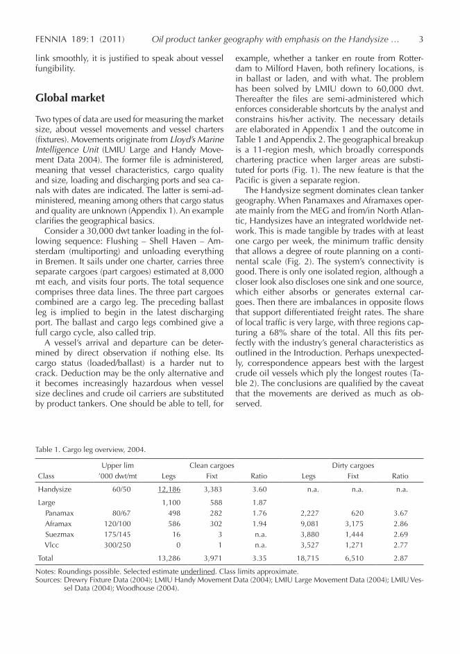
Neste Oil’s operations are evaluated best against its competitors. Most of them were in Scandinavia or the Balticum, or at least exported through its ports (Table 6). Available information calls for care in interpretation. Roughly 60% of Neste’s export tonnage was shipped in vessels small enough to escape the Handysize definition, and the Neste and LMIU data sets are only broadly comparable (Appendix 1). All quoted refineries supplied the lo-cal market, but exports could easily approach the 50/50 mark. Mažeikiu Nafta in Lithuania and Preem in Sweden being typical cases (Preem AB 2004; Maižeikiu Nafta 2005). Russian exports pose the main dilemma because no refinery was on the seaboard (Maižeikiu Lithuanian-owned) and most were far inland. Kirishi is only 110 km from St. Petersburg but Moscow, Yaroslavl and


Rjazan are already 650–900 km from Baltic ports. It is very much a question of rail tariffs, which at such distances comprise up to 10%–12% of the fob cost and are three times higher than pipeline tariffs (Byev et al. 2006: 88–89). Klaipeda even re-ceived crude oil from Kazahstan, a distance of 3,000 km. The terminal is a subport of Klaipeda and exports are registered there. The Gdansk refin-ery was half the size of Sköldvik (Atlas... 2003; George 2003; Lorimer 2003; Stell 2003; Tykkyläi-nen 2003; LMIU Handy Movement Data 2004; Byev et al. 2006: 38–40, 89–90; Surgutneftegaz 2009). Neste was thus in a favorable competitive position in the Baltic (Fig. 3). Competition intensi-fied beyond the Baltic but it was less advanced technologically than one might expect1. Neste considered only the Swedes and Immingham as equals (Harki 2009b). The market shares in the core market Baltic–North Sea, Biscaya–Western Mediterranean tended to stay within 85%–90%, whereas the pull of North America grew on the

North Sea and the relatively modest market in Québec and Maritime Provinces absorbed more than New York (Fig. 3). But geographical closeness alone was not sufficient. Technical excellence tuned to market preferences carried much weight, particularly in California, notwithstanding the dis-tance (9,000 nm) and Panama Canal charges ($140,000). Neste also excelled there with three 35,000–40,000 mt cargoes of high-grade gasoline.

Globally, California is the cul-de-sac of oil logis-tics, with 15% of supplies coming from the out-side, from Alaska and via refineries in the Vancou-ver area. It is comparatively isolated from the Car-ibbean by the congested Panama Canal and from the Asia Pacific by the vast spaces of the ocean. Yet, Korea and Japan were the closest overseas sources and also Neste Oil’s keenest competitors. The surcharge toward Korea, “only” 5,000 nm dis-tant, was 24 $/mt, which wiped away the calcula-tory 23 $/mt refinery margin1. An important reason for the comparatively low Korean presence,

Table 6. Handysize oil product exports from some refineries in NW Europe, 2004.

Company/class Refin. Intake Maritime cargos by Region Cargosno bbl/day mmt 1–3 6–8 Rest Trans

% % %

Neste Oil (Sköldvik, Naantali) 2 252 5.0 419

Aframax 84,000 dwt 0.1 2 Panamax 67,000 dwt 0.4 8 Handysize 15–59,999 dwt 2.4 138 Small 10–14,999 dwt 1.4 129 Mini 2–9,999 dwt 0.7 142

LMIU 15–59,999 dwtFinland (Sköldvik, Naantali) 2 252 1.7 12 85 3 127North Baltic (Russia, Estonia) 1 336 17.1 2 97 1 702Mid Baltic (Latvia, Litva, Kalin.) 1 260 13.2 8 89 4 576Poland (Gdansk) 1 90 1.1 6 85 9 54Denmark (Kalundb, Fredericia) 2 176 1.3 9 90 2 58Sweden (Brofjord, Gothenburg) 3 406 5.1 11 85 4 218Norway (Mongstad, Slagen) 2 310 3.0 11 87 2 145UK (Immingham) 2 447 5.2 17 78 5 195

All LMIU 14 2,277 47.7 7 92 2 2,075

World, Seaboard 275 53,600 781.3 28,500

Notes: Domestic shipments excluded. Canary Isl., Puerto Rico, Virgin Isl. and similar are considered foreign territories. Neste data cargos and tonnes (dwt = 0.8 mt). LMIU data non-treated (100%) transits. Percentages from transits. Roundings possible. Region 1-3 refers to North American Atlantic Coast & Caribbean and Region 6-8 to Baltic & North Sea & Biscaya & W. Mediterranean. They originate from a 26-region mesh. Nynäshamn refinery specialized in bitumen and is outside this study. Global figures without scaling (App. 1).Sources: Stell (2003); LMIU Handy Movement Data (2004); Harki (2009a), Laulajainen (2010, Fig. 4).


450,000 mt or 3% of the market, must have been the refineries’ modest technical sophistication (LMIU Handy Movement Data 20042). Of course, sophistication becomes expensive and is never an end in itself but a vehicle to gain meaningful com-petitive advantage.

Fungibility

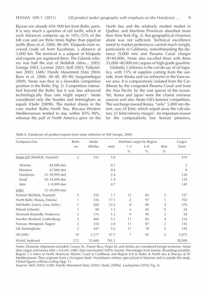
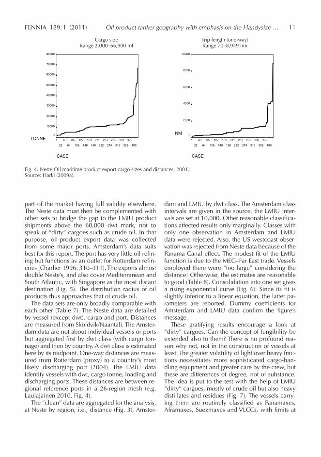
Most of Neste’s cargoes were quite small. Only 60% exceeded the approximate Handysize lower boundary 12,000 mt (15,000 dwt; Fig. 4). A full cargo often consisted of several qualities, up to five, but it was unusual that a vessel discharged in more than one port, and then close to each other. The smallest cargoes, down to 2,000 mt (2,500 dwt), were chemicals, bitumen and bunkers. Fuel

oil cargoes could also be small, 3,000–4,000 mt, but only when channels and ports were shallow. The total share of non-clean cargoes was 3.5%. Distant shipments were always gasoline. Loading in both Sköldvik and Naantali for the same trip was unusual. Distances reflect the refinery loca-tions at the far end of the Baltic. Three zones can be outlined: Northern Europe up to 2,000 nm (one-way), East Coast North America (ECNA) about 4,000 nm and Los Angeles 9,000 nm (Fig. 4).

Cargo size and distance seem to change in tan-dem, tying together the small end of the market and the rest. The link is weak when individual car-goes are considered, but quite strong when trips are aggregated by cargo size and distance. It may even be possible to speak about the fungibility of the oil tanker market; observations made in one

N P Pr

P = PorvooN = NaantaliPr = Primorsk

NESTE OILproduct exports

650

330110

‘000 tonnes

1470

1080

700

60

110

460

Fig. 3. Neste Oil maritime product exports, 2004. Source: Harki (2009a).

Fig. 3. Neste Oil maritime product exports, 2004.Source: Harki (2009a).


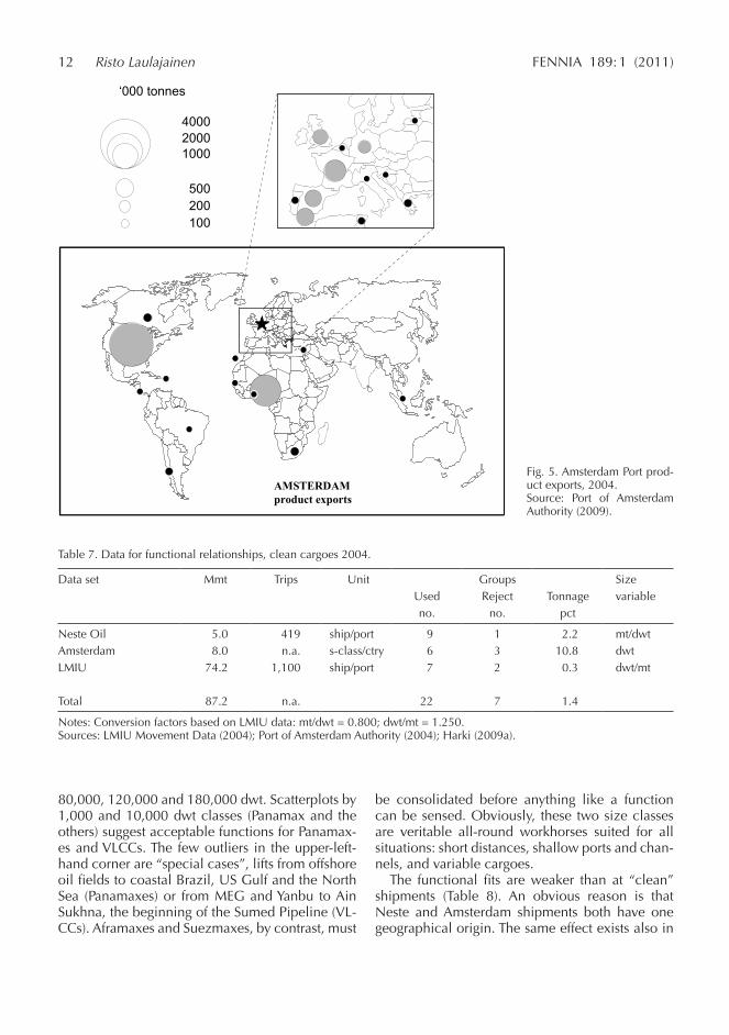
part of the market having full validity elsewhere. The Neste data must then be complemented with other sets to bridge the gap to the LMIU product shipments above the 60,000 dwt mark, not to speak of “dirty” cargoes such as crude oil. In that purpose, oil-product export data was collected from some major ports. Amsterdam’s data suits best for this report. The port has very little oil refin-ing but functions as an outlet for Rotterdam refin-eries (Charlier 1996: 310–311). The exports almost double Neste’s, and also cover Mediterranean and South Atlantic, with Singapore as the most distant destination (Fig. 5). The distribution radius of oil products thus approaches that of crude oil.

The data sets are only broadly comparable with each other (Table 7). The Neste data are detailed by vessel (except dwt), cargo and port. Distances are measured from Sköldvik/Naantali. The Amster-dam data are not about individual vessels or ports but aggregated first by dwt class (with cargo ton-nage) and then by country. A dwt class is estimated here by its midpoint. One-way distances are meas-ured from Rotterdam (proxy) to a country’s most likely discharging port (2004). The LMIU data identify vessels with dwt, cargo tonne, loading and discharging ports. These distances are between re-gional reference ports in a 26-region mesh (e.g. Laulajainen 2010, Fig. 4).

The “clean” data are aggregated for the analysis, at Neste by region, i.e., distance (Fig. 3), Amster-

dam and LMIU by dwt class. The Amsterdam class intervals are given in the source, the LMIU inter-vals are set at 10,000. Other reasonable classifica-tions affected results only marginally. Classes with only one observation in Amsterdam and LMIU data were rejected. Also, the US westcoast obser-vation was rejected from Neste data because of the Panama Canal effect. The modest fit of the LMIU function is due to the MEG–Far East trade. Vessels employed there were “too large” considering the distance! Otherwise, the estimates are reasonable to good (Table 8). Consolidation into one set gives a rising exponential curve (Fig. 6). Since its fit is slightly inferior to a linear equation, the latter pa-rameters are reported. Dummy coefficients for Amsterdam and LMIU data confirm the figure’s message.

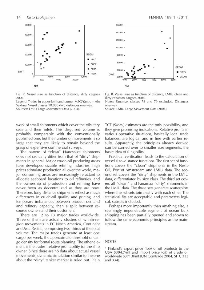
These gratifying results encourage a look at “dirty” cargoes. Can the concept of fungibility be extended also to them? There is no profound rea-son why not, not in the construction of vessels at least. The greater volatility of light over heavy frac-tions necessitates more sophisticated cargo-han-dling equipment and greater care by the crew, but these are differences of degree, not of substance. The idea is put to the test with the help of LMIU “dirty” cargoes, mostly of crude oil but also heavy distillates and residues (Fig. 7). The vessels carry-ing them are routinely classified as Panamaxes, Aframaxes, Suezmaxes and VLCCs, with limits at

Cargo size Trip length (one-way) Range 2,000 – 66,900 mt Range 70 – 8,949 nm

CASE

400

379

358

337

316

295

274

253

232

211

190

169

148

127

106

85

64

43

22

1TONNE

80000

70000

60000

50000

40000

30000

20000

10000

0

CASE

400

379

358

337

316

295

274

253

232

211

190

169

148

127

106

85

64

43

22

1

NM

10000

8000

6000

4000

2000

0

Fig. 4. Neste Oil maritime product export cargo sizes and distances, 2004. Source: Harki (2009a).

Cargo size Trip length (one-way) Range 2,000–66,900 mt Range 70–8,949 nm

Fig. 4. Neste Oil maritime product export cargo sizes and distances, 2004.Source: Harki (2009a).


AMSTERDAMproduct exports

‘000 tonnes

20004000

1000

100200500

Fig. 5. Amsterdam Port product exports, 2004. Source: Port of Amsterdam Authority (2009).

Fig. 5. Amsterdam Port prod-uct exports, 2004.Source: Port of Amsterdam Authority (2009).

Table 7. Data for functional relationships, clean cargoes 2004.

Data set Mmt Trips Unit Groups SizeUsed Reject Tonnage variableno. no. pct

Neste Oil 5.0 419 ship/port 9 1 2.2 mt/dwtAmsterdam 8.0 n.a. s-class/ctry 6 3 10.8 dwtLMIU 74.2 1,100 ship/port 7 2 0.3 dwt/mt

Total 87.2 n.a. 22 7 1.4

Notes: Conversion factors based on LMIU data: mt/dwt = 0.800; dwt/mt = 1.250.Sources: LMIU Movement Data (2004); Port of Amsterdam Authority (2004); Harki (2009a).

80,000, 120,000 and 180,000 dwt. Scatterplots by 1,000 and 10,000 dwt classes (Panamax and the others) suggest acceptable functions for Panamax-es and VLCCs. The few outliers in the upper-left-hand corner are “special cases”, lifts from offshore oil fields to coastal Brazil, US Gulf and the North Sea (Panamaxes) or from MEG and Yanbu to Ain Sukhna, the beginning of the Sumed Pipeline (VL-CCs). Aframaxes and Suezmaxes, by contrast, must

be consolidated before anything like a function can be sensed. Obviously, these two size classes are veritable all-round workhorses suited for all situations: short distances, shallow ports and chan-nels, and variable cargoes.

The functional fits are weaker than at “clean” shipments (Table 8). An obvious reason is that Neste and Amsterdam shipments both have one geographical origin. The same effect exists also in


Table 8. Vessel size as function of distance, clean and dirty cargoes 2004.

Data set Obs. R-sqr SEE Coefficients Interc.(adj) Dist Amst LMIU

CleanNeste Oil 9 0.919 4,649 10.16 4,794Amsterdam 6 0.940 3,145 8.84 –207LMIU 7 0.666 11,703 18,74 9,527

All clean 22 0.956 8,294 11.04 –7,335 41,202 3,352

Dirty (LMIU)Panamax 18 0.468 3,862 5.95 56,582AfraSuez 80 0.304 21,372 10.44 98,215Vlcc 15 0.764 30,886 23.12 136,904

All dirty 26 0.839 37,700 32.42 68.824

LMIUDirty (Pana)/Clean 25 0.767 7,809 10.74 46,402

Notes: Distance one-way, nautical miles. All functions linear. Coefficients significant at about 1% risk.Excluded dirty classes: Panamax 78, 79 (not in All dirty); Vlcc 36, 40, 42.Sources: LMIU Movement Data (2004); Port of Amsterdam Authority (2004); Harki (2009a).

NM

6000500040003000200010000

DWT

140000

120000

100000

80000

60000

40000

20000

0

-20000

DATA

NESTE

LMIU

AMST

Fig. 6. Vessel size as function of distance, clean cargoes 2004. Legend: Large marker Neste Oil; small marker above LMIU; small marker below

Amsterdam Port. Vessel classes, see text. Distances one-way. Sources: LMIU Movement Data (2004); Port of Amsterdam Authority (2004); Harki

(2009a).

Fig. 6. Vessel size as function of distance, clean cargoes 2004.Legend: Large marker Neste Oil; small marker above LMIU; small marker below Amsterdam Port. Vessel classes, see text. Distances one-way.Sources: LMIU Movement Data (2004); Port of Amsterdam Authority (2004); Harki (2009a).

“dirty” shipments: MEG dominates large crude oil cargoes and the effect is visible in the good fit of the VLCC equation. When all the size classes are consolidated and the VLCC outliers above exclud-ed, the joint function is quite acceptable. Not un-

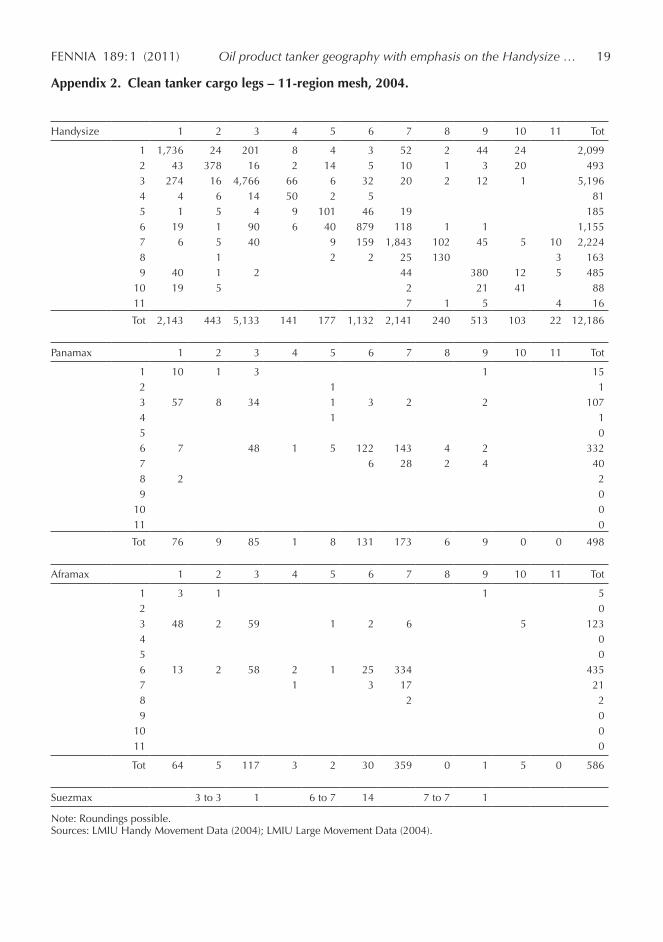
surprisingly, the parameters deviate from the “clean” parameters, a rather crucial test of fungi-bility. Therefore, the “clean” LMIU and “dirty” Panamax data are joined into one set, scatterplot prepared and parameters re-estimated. The “dirty” half has two-thirds of observations but the “clean” half has a wider range (Fig. 8). Therefore, it is im-possible to decide which one dominates. Rather, the “clean” set continues the “dirty” set. This can be interpreted as a kind of proof for the fungibility.

Conclusion

This report took to its task to create a holistic idea about the “clean” oil product shipping market, particularly the thousands of smallish tankers that do not meet the minimum size criterion of a Pan-amax vessel, 60,000 dwt (50,000 mt). To that pur-pose, it has combined existing global and local databases and created from them a tangible idea about the “clean” market, described its structure and commented on its rationality. Because the un-derlying data are not readily available, the results have been extensively tabulated.

Handysize product tankers apparently dominate shipments exceeding 3,000 nm, an opinion based on widely distributed spot fixtures. These accumu-late on large trades and overshadow the dense net-


work of small shipments which cover the tributary seas and their inlets. This disguised volume is probably comparable with the conventionally published one, but the number of movements is so large that they are likely to remain beyond the grasp of expensive commercial surveys.

The pattern of “clean” Handysize shipments does not radically differ from that of “dirty” ship-ments in general. Major crude-oil producing areas have developed sizable refining industries, high prices stimulate production all over the world, ma-jor consuming areas are increasingly reluctant to allocate seaboard locations to oil refineries, and the ownership of production and refining have never been as decentralized as they are now. Therefore, long-distance shipments reflect as much differences in crude-oil quality and pricing, and temporary imbalances between product demand and refinery capacity, than a split between re-source owners and their customers.

There are 12 to 13 major trades worldwide. Three of them are actually clusters of within-re-gion movements in EC North America, Continent and Asia Pacific, comprising two-thirds of the total volume. The major trades generate at least one cargo per week, the approximate threshold of car-go density for formal route planning. The other ele-ment is the trades’ relative profitability for the ship owner. Since there are no data about actual vessel movements, dynamic simulation similar to the one about the “dirty” tanker market is ruled out. Plain

TCE ($/day) estimates are the only possibility, and they give promising indications. Relative profits in various operative situations, basically local trade balances, are logical and in line with earlier re-sults. Apparently, the principles already derived can be carried over to smaller size segments, the basic idea of fungibility.

Practical verification leads to the calculation of vessel size–distance functions. The first set of func-tions covers the “clean” shipments in the Neste Oil, Port of Amsterdam and LMIU data. The sec-ond set covers the “dirty” shipments in the LMIU data, differentiated by size class. The third set cov-ers all “clean” and Panamax “dirty” shipments in the LMIU data. The three sets generate scatterplots where the subsets join neatly with each other. The statistical fits are acceptable and parameters logi-cal, subsets included.

Perhaps more importantly than anything else, a seemingly impenetrable segment of ocean bulk shipping has been partially opened and shown to follow the same economic principles as the main-stream.

NOTES

1 Finland’s export price (fob) of oil products to the USA $394.7/mt and import price (cif) of crude oil worldwide $371.8/mt (UN Comtrade 2004, SITC 333 and 334).

NM

1200010000

80006000

40002000

0

DWT

500000

400000

300000

200000

100000

0

SEGM

VLCC

SUEZ

AFRA

PANA

Fig. 7. Vessel size as function of distance, dirty cargoes 2004. Legend: Trades in upper-left-hand corner MEG/Yanbu – Ain Sukhna.

Vessel classes 10,000 dwt, distances one-way. Sources: LMIU Large Movement Data (2004).

Fig. 7. Vessel size as function of distance, dirty cargoes 2004.Legend: Trades in upper-left-hand corner MEG/Yanbu – Ain Sukhna. Vessel classes 10,000 dwt, distances one-way.Sources: LMIU Large Movement Data (2004).

NM

600050004000300020001000

DWT

130000

120000

110000

100000

90000

80000

70000

60000

SEGM

DIRTY

CLEAN

Fig. 8. Vessel size as function of distance, LMIU clean and

dirty Panamax cargoes 2004. Notes: Panamax classes 78 and 79 excluded. Distances one-way. Source: LMIU Large Movement Data (2004).

Fig. 8. Vessel size as function of distance, LMIU clean and dirty Panamax cargoes 2004.Notes: Panamax classes 78 and 79 excluded. Distances one-way.Source: LMIU Large Movement Data (2004).


2 A rule-of-thumb indicator for technological excel-lence is the total of catalytic treatment charges out of the total crude oil intake. The percentage can be a bit vague because some streams are consecutive while others are parallel. It was 188% at the Conoco Im-mingham refinery, 136% at Sköldvik, 130% at Shell Gothenburg and 116% at Preem Brofjorden. The cor-responding US figures were East Coast 142%, Gulf Coast 146% and California 155%. South Korea’s most active refineries in Onsan and Ulsan had 81% and 51%, respectively (Stell 2003; see also Laulajain-en & Stafford 1995, Figure 5.32).

ACKNOWLEDGEMENTS

Acknowledgement is due to Wally Mandryk (Lloyd’s Marine Intelligence Unit), Brendan Martin (Gibson Shipbrokers), Susan Oatway (Drewry Shipping Con-sultants), Robert Porter (Worldscale Association, Lon-don) and Abbass Vashoeey (Port of Amsterdam Au-thority) for complimentary data and advice, as well as Howard Stafford (University of Cincinnati) for help in mining published data sources. Special thanks are due to Jan van Weesep, Editor-in-Chief of TESG, Utrecht, whose analytical stringency superseded the author’s.

REFERENCES

Atlas zheleznyh i avtomobiljnyh dorog 2003. AST Astrelj, Moscow.

Baltic Clean Tanker Index (BCTI) 2004. Baltic Ex-change, London.

Blas J 2009. Narrow oil spreads put pressure in mod-ern refineries. Financial Times, 24, 23 June.

Byev D, Novikova A, Zelenina J, Zinkina I & Gubano-va O 2006. Logistika neftenalivnyh perevozok. SeaNews, Saint Petersburg.

Cellineri LE 1976. Seaport Dynamics, a Regional Per-spective. Lexington Books, Lexington.

Chapman K 1991. The International Petrochemical Industry. Blackwell, Oxford.

Charlier J 1996. The Benelux seaport system. Tidschrift voor Economische en Sociale Geografie 87: 4, 310–321.

Drewry Fixture Data 2004. Drewry Shipping Consul-tants, London.

Fagerholt K 2004. A computer-based decision sup-port system for vessel fleet scheduling – experi-ence and future research. Decision Support Sys-tems 37: 1, 35–47.

Fortum Ltd 2004. Annual Report. <www.fortum.com/webannualreport2004> 12.4.2010.

George N 2003. Trucks trundle in from Russia while oil pipeline stays closed. Financial Times, 3, 25 November.

Glen D & Martin B 2002. The tanker market: current structure and economic analysis. In Grammenos CTh (ed). The Handbook of Maritime Economics and Business, 215–279. LPP, London.

Harki M 2009a. Exports of oil products 2004. Neste Oil, Helsinki.

Harki M 2009b. Phone interview. Neste Oil, Helsin-ki. 4 March.

Isserlis L 1938. Tramp shipping cargoes and freights. Journal of the Royal Statistical Society 101: 1, 53–146.

Laulajainen R 2006. The Geographical Foundations of Dry Bulk Shipping. Gothenburg School of Busi-ness, Economics and Law, Gothenburg.

Laulajainen R 2007. The geographical foundations of tanker (dirty) shipping. Maritime Policy and Man-agement 34: 6, 553–576.

Laulajainen R 2008. Operative strategy in tanker (dirty) shipping. Maritime Policy and Manage-ment 35: 3, 315–341.

Laulajainen R 2010. Geography sets the tone to tramp routing. International Journal of Shipping and Transport Logistics 2: 4, 364–382.

Laulajainen R 2011. Port-turntable, the foreland con-cept repackaged. Manuscript.

Laulajainen R & Stafford HA 1995. Corporate Geo-graphy. Kluwer, Dordrecht.

LMIU Handy Movement Data (semi-administered) 2004. Lloyd’s Marine Intelligence Unit, London.

LMIU Large Movement Data (administered) 2004. Lloyd’s Marine Intelligence Unit, London.

LMIU Vessel Data 2004. Lloyd’s Marine Intelligence Unit, London.

Lorimer A 2003. Russia’s new oil gateways. Lloyd’s Shipping Economist, 15–18, December.

Maižeikiu Nafta 2005. <http://en.wikipedia.org/wiki/Ma> 12.4.2010.

Matheson MH 1955. The hinterlands of Saint John. Geographical Bulletin 5–6, 65–102. Geographi-cal Branch, Department of Mines and Technical Surveys, Ottawa.

Musso E & Marchese U 2002. Economics of shortsea shipping. In Grammenos CTh (ed). The Handbook of Maritime Economics and Business, 280–304. LPP, London.

Nossum B 1996. The Evolution of Dry Bulk Shipping 1945–1990. Fearnley & Egers, Oslo.

Port of Amsterdam Authority 2004. Trade statistics by country, unpublished.

Preem AB 2004. Annual Report. <www.preem.se/up-load/pdf> 12.4.2010.

Rodgers A 1958. The port of Genova: external and internal relations. Annals of the Association of American Geographers 48: 4, 319–351.

Stell J (ed) 2003. Worldwide refining survey. Oil & Gas Journal, 1–41, 22 December.

Stopford M 1997. Maritime Economics. Routledge, London.

Surgutneftegaz 2009. General information. <www.surgutneftegaz.ru/en/oil/about/> 12.4.2010.


Tykkyläinen M 2003. North-west Russia as a gateway in Russian energy geopolitics. Fennia 181: 2, 145–177.

UN Comtrade 2004. United Nations Commodity Sta-tistics Database, SITC 333 and 334, New York. <http://comtrade.un.org.ezproxy.ub.gu.se> 12.4.2010.

Verlaque Ch 1975. Géographie des transports mariti-mes. Doin, Paris.

Wijnolst N, Peters C & Liebman P (eds) 1993. Euro-pean Shortsea Shipping. LLP, London.

Woodhouse Z (ed) 2004. Tanker Book. E.A. Gibson Shipbrokers, London.

Worldscale 2004. New Worldwide Tanker Nominal Freight Scale. Worldscale Association (London)Ltd & Worldscale Association (NYC) Inc.


A large volume of mineral oil product (“clean”) shipments are made by Handysize vessels of 15,000–59,999 dwt. When the question is sharp-ened to a percentage, only guesstimates can be given. Lloyd’s Marine Intelligence Unit gives a fairly reliable estimate of the “Large” vessel class-es, 60,000 dwt and over. In addition, it has com-piled a semi-administered file of the Handysize class (LMIU Handy Movement Data 2004). About the classes below 15,000 dwt nothing is available worldwide, and it is unlikely that they will be cov-ered by a global census in the near future. Yet, in the Neste Oil database these classes make two-thirds of export legs and one-third of tonnage (Ta-ble 6).

The best that can be done currently is to make use of the Handysize data. Its semi-administered state means many things. A line in the data file ag-gregates 1 to 95 individual “transits” (“legs”/“trips” in this author’s terminology). Analysis of individual legs is thereby ruled out. The emphasis is on ocean traffic and legs from/to/within Great Lakes are also excluded here. Remain 49,200 legs. Liquid car-goes other than mineral oil products are included, such as liquid ammonia and vegetable oils. Ready examples are 100 legs from Ambes, Garonne estu-ary, and 157 legs from Pasir Gudang, Johore Strait. Such loading ports should be excluded here, case by case, but the workload becomes prohibitive. One goes the other way. Since mineral oil prod-ucts originate from corresponding refineries, the seaboard (port) refineries identify important ori-gins with a total of 26,600 legs. One half of them are guesstimated to be cargo legs. Following the same reasoning, 1,400 relevant cargo legs origi-nate from the ports of the former Soviet Union. These ports seldom have refineries that are found far inland at major oil fields and consumption centers. Distances of 1,000–2,000 km by pipeline or rail are quite usual. Return legs from foreign re-finery destinations to these export ports are 1,300, roughly in balance with calculatory cargo legs.

The small size of some port refineries, below 50 bbl/d, may raise doubts about their true export ca-pacity. They are given the benefit of the doubt and retained, a total of 2,000 cargo legs. For example, Amsterdam has only a 10 bb/d refinery but is con-nected by pipeline with Rotterdam’s refineries and handles a large share of its exports (Charlier 1996: 310–311). Because the cargo status of individual

leg strings is not known, multiporting cannot be identified. Multiporting raises the number of port visits 16%–17% in the larger “clean” size classes and the “dirty” tanker segment and should also ap-ply here. The corresponding discount reduces the number of calculatory mineral oil product legs to 12,300.

A factor of unknown magnitude are cargoes swapped between refinery ports, be it for quality difference or company affiliation. They, naturally, are very real ones but complicate the cargo/ballast split. They are identified best by asking cargo own-ers directly during data collection. Observations based on vessel draught are unreliable because pipelines connect refineries and tank farms into vast networks.

All legs 49,166

From seaboard refinery ports 26,568Cargo from seaboard refineries, 50% 13,284From former Soviet ports 2,796Cargo from former Soviet ports, 50% 1,398All cargo 14,682Discount for multiporting, 17% –2,496Oil product legs, 244 per week 12,186Fixtures 3,383Ratio 3.60

Note: Figures rounded.

The cargo legs are tabulated within the 11-region mesh and the cell elements divided by 50 to arrive at average full week cargo flows between the re-gions. The Ratio Legs/Fixtures is compared with clean and dirty vessel classes of 60,000 dwt and above (Table 1). Compatibility is acceptable.

This is how things look at the global level. But it is a good policy to also have a look at the national level when there is an opportunity to do so. Fin-land is a good example, due to the availability of Neste Oil’s export statistics and the author’s famili-arity with local conditions. The LMIU Handy Movement Data (2004) transits are disaggregated as follows. “Refinery” means a refinery location rather than a company or plant.

Appendix 1. LMIU Handysize Movement File, 2004.


From domestic Refinery Other TotalAll Oil All Oil Oil

To foreign refinery 40 40 5 0 40foreign other 43 43 42 0 43domestic refinery 25 13 22 0 13domestic other 19 10 20 10 20

Total 127 106 89 10 116less 50%, remains 63.5 44.5less 17%, remains 53 37 90

Difference 26

Notes: Estimates underlined in the body of table subject to discussion. Direct total estimates in bold. Strictly calculatory total estimate in normal text. Shipments from foreign refineries handled in the context of appropriate countries.

“Refinery” is the source of most oil product car-goes. The two first elements 40 + 43 correspond formally to Neste Oil’s export cargoes in the Handysize class (Table 6). But Neste’s own figure is 138. The difference originates from Bremen (44) and Kalundborg (11) where the vessels were very close to the 15,000 dwt limit used by LMIU. Since the conversion factor from mt to dwt is an approx-imation, the result falls easily within the measure-ment error. Therefore, both counts are used in par-allel as seems fit (Table 6). Transits between the refineries, 25 legs, are inventory balancing or swaps of intermediates and the share of cargo legs can vary within 50%–100%. The smallest possibil-

ity is adopted here. The remaining 19 legs are de-liveries to coastal depots, own or customers’. The corresponding 22 ballast legs are in the “Other” column on the way to “domestic refinery.” The 20 “domestic other” originate from companies other than Neste and have some ballasting matches be-tween port pairs. They need not be oil cargoes at all, but if they are, trader activity is again a possi-bility.

The grand total of 116 cargo legs is thus 26 legs larger than the calculatory total estimate of 90. The calculatory route can be used in a global discus-sion. A national discussion is preferably based on direct observation.


Appendix 2. Clean tanker cargo legs – 11-region mesh, 2004.

Handysize 1 2 3 4 5 6 7 8 9 10 11 Tot

1 1,736 24 201 8 4 3 52 2 44 24 2,0992 43 378 16 2 14 5 10 1 3 20 4933 274 16 4,766 66 6 32 20 2 12 1 5,1964 4 6 14 50 2 5 815 1 5 4 9 101 46 19 1856 19 1 90 6 40 879 118 1 1 1,1557 6 5 40 9 159 1,843 102 45 5 10 2,2248 1 2 2 25 130 3 1639 40 1 2 44 380 12 5 485

10 19 5 2 21 41 8811 7 1 5 4 16

Tot 2,143 443 5,133 141 177 1,132 2,141 240 513 103 22 12,186

Panamax 1 2 3 4 5 6 7 8 9 10 11 Tot

1 10 1 3 1 152 1 13 57 8 34 1 3 2 2 1074 1 15 06 7 48 1 5 122 143 4 2 3327 6 28 2 4 408 2 29 0

10 011 0

Tot 76 9 85 1 8 131 173 6 9 0 0 498

Aframax 1 2 3 4 5 6 7 8 9 10 11 Tot

1 3 1 1 52 03 48 2 59 1 2 6 5 1234 05 06 13 2 58 2 1 25 334 4357 1 3 17 218 2 29 0

10 011 0

Tot 64 5 117 3 2 30 359 0 1 5 0 586

Suezmax 3 to 3 1 6 to 7 14 7 to 7 1

Note: Roundings possible.Sources: LMIU Handy Movement Data (2004); LMIU Large Movement Data (2004).

oil product tanker geography with emphasis on the handysize segment

Documents