oil reservoir properties estimation by fuzzy-neural...

Memoirs of the Faculty of Engineering, Kyushu University, Vol.67, No.3, September 2007

Oil Reservoir Properties Estimation by Fuzzy-Neural Networks

by

Trong Long HO* and Sachio EHARA†

(Received August 16, 2007)

Abstract

Porosity and permeability are two fundamental reservoir properties which relate to the amount of fluid contained in a reservoir and its ability to flow. These properties have a significant impact on petroleum fields operations and reservoir management. Up to now, more than twenty reservoirs have been found in basement rocks all over the world, which were known as un-usual reservoir. They were named un-usual reservoir because of the small number are compared with clastic and carbonate reservoirs. Study on basement reservoir always is difficult task, especially estimation of reservoir properties due to complex nature of the geological model. In this paper, we suggest an efficient method to determine reservoir properties from well log by using fuzzy logic and neural networks. The ranking technique based on fuzzy logic is used for noise rejection of training data for neural networks. By learning the nonlinear relationship between selected well logs and core measurements, the neural network can perform a nonlinear transformation to predict porosity or permeability with high accuracy. The approach is demonstrated with an application to the well data in A2-VD prospect, Southern offshore Vietnam. The results show that this technique can make more accurate and reliable reservoir properties estimation than conventional computing methods. The study plays an important role in projects of development of basement reservoirs in the future. Keywords: Porosity, Permeability, Fuzzy logic, Artificial neural networks, Well log, Basement reservoir, A2-VD prospect

1. Introduction

Vietnam is one of the countries having oil in basement rock. Hydrocarbons were found in fractured basement rock in more than twenty basins all over the world. Such basins are found in

* Graduate Student, Department of Earth Resources Engineering † Professor, Department of Earth Resources Engineering

118 T.L. HO and S. EHARA

Algeria, Argentina, Brazil, Canada, Chile, China, Egypt, India, Indonesia, Russia, United Kingdom, United States and Vietnam (Sircar, 2004). In Vietnam, basement reservoirs are major reservoirs which are providing over 90% of the production rate. Therefore, the basement reservoir has become an attractive target and has been paid a great attention for investigation.

However, because of complex nature of the geological model and the small number of fractured reservoirs compared with clastic and carbonate reservoirs over the world, the researches on the basement reservoir are still limited and the understanding of the basement reservoir is also difficult. Such reservoir was named an “unusual reservoir”.

The area that forms the scope of this study lies in the southern offshore Vietnam, Cuu Long basin, which is ranked first among petroleum potential basins (Fig. 1). Because of its rich lacustrine source rock and unusual fractured basement reservoir, it has become well known not only in Vietnam but also in South-East Asia. The Cuu Long basin is a Tertiary rift basin on the southern shelf of Vietnam. It covers an area of approximately 25,000 km2 (250 km x 100 km). The basin was formed during the rifting in Early Oligocene. Late Oligocene to Early Miocene inversion intensified the fracturing of basement and made it an excellent reservoir.

Basement rock of the Cuu Long basin includes magmatic rocks such as granite, granodiorite, quarzt-diortie, monzodiorite, diorite, and meta-sediments; in them, granite is the basement rock of A2-VD prospect (Dong et al., 2001). The outstanding feature of the petroleum system in this basin is the combination of the Oligocene source rocks with the Mesozoic basement reservoir (Dien, 2001). Many descriptions and analysis of this type of basement reservoir showed that the porosity of the basement reservoir consisted mainly of fractures and vug-cavities due to various processes such as tectonic activities, weathering, hydrothermal and volumetric shrinkage of cooling magma. (Dong et al., 1991, 1994, 1998, 1999; San et al.,1997; Vinh, 1999, Dien, 2001). Among them, the tectonic activity and the hydrothermal processes are practically the main factors that control the porosity of the fracture systems. Recent studies (Cuong, 2001; Schmidt, 2003) proved that the compression event that occurred during Late Oligocene reactivated the pre-existing faults/fractures and created effective porosity inside the basement.

Basin analysis and evolution of basement highs showed that the most effective porosity of the basement reservoirs has a relationship with many factors relating to the basement highs and surrounding sedimentary sequences. This special combination consists of the volumetric shrinkage due to the diagenesis of the Paleogene sedimentary sequences distributed in grabens up-lap slopes of basement highs, the breakable of rigid-brittle and non-bedding basement highs on the hangingbranch of fault systems, and the accumulated capping-mass of Miocene to Quaternary sediments on top the basement high (i.e. the highest area of the basement). The break of buried crystalline basement rocks has lead to the formation of a series of fractures and vugs with diverse shape and size in the environment where there was no filling sedimentary materials and water. This is the most effective porosity type of the basement reservoirs in Cuu Long basin.

Permeability of the basement reservoir in Cuu Long basin is mainly influenced by fracture system, and the high permeability zone is related to fracture zone and shows the fracture development area. Therefore, porosity and permeability are two key parameters of the A2-VD prospect in Vietnam. They are very valuable information for reservoir simulation and developing plans of the prospect in the future. In this paper we will present a method to predict porosity and permeability in basement rock from well log data by using fuzzy logic and neural network, and a case study in the A2-VD prospect, southern offshore Vietnam.

Oil Reservoir Properties Estimation by Fuzzy-Neural Networks 119

Fig. 1 Location of the studied area.

2. Fuzzy-Neural Networks Recognition

Fuzzy logic was first developed by Zadeh (1988) in the mid-1960s for representing uncertain

and imprecise knowledge. It provides an approximate but effective means of describing the behavior of systems that are too complex, ill-defined, or not easily analyzed mathematically. Fuzzy variables are processed using a system called a fuzzy logic controller. It involves fuzzification, fuzzy inference, and defuzzification. The fuzzification process converts a crisp input value to a fuzzy value. The fuzzy inference is responsible for drawing conclusions from the knowledge base. The defuzzification process converts the fuzzy control actions into a crisp control action.

When anything becomes too complex to fully understand, it becomes uncertain. The more complex something is, the more inexact or "fuzzier" it will be. Fuzzy logic provides a very precise approach for dealing with uncertainty which grows out of the complexity of human behavior. Among fuzzy logic techniques, fuzzy ranking is a tool to select variables that are globally related, it allows ranking the level of the globally relationships. Fuzzy ranking is known as a very efficient tool for removing noise of data by evaluating globally relationship between variables.

One of the most successfully applications of artificial neural network is pattern recognition, but the limitation of the neural networks is that their success strongly depends on noise of training data set. Therefore, in this study, we suppose to use fuzzy ranking to reject noise from training data set of the neural network, which is called fuzzy-neural network. The fundamental idea of the fuzzy-neural network approach is shown in Fig. 2.


Fig. 2 Fundamental of the fuzzy-neural network. Consider a data pair (x, y) where x is the event and y is the reaction. The problem is to predict y

when x changes slightly, in a neighbourhood close to x. The fuzzy membership function of (x, y) gives a local prediction of y, according to the information from only (x, y). The fuzzification of the data is done with Gaussian function. Fuzzy membership function is defined as follows;

i

2i

i y.b

xxexp)x(F

, (1)

where b defines the shape of the fuzzy membership curves and is about 10% of data set range. A fuzzy curve function is used to rank noisy data. The fuzzy curve function gives a global prediction y because it consists of the sum of the local predictions (fuzzy membership functions). Fuzzy curve function FC(x) is defined as follows;

n

1iii

n

1ii

y/)x(F

)x(F)x(FC . (2)

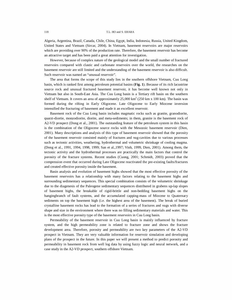
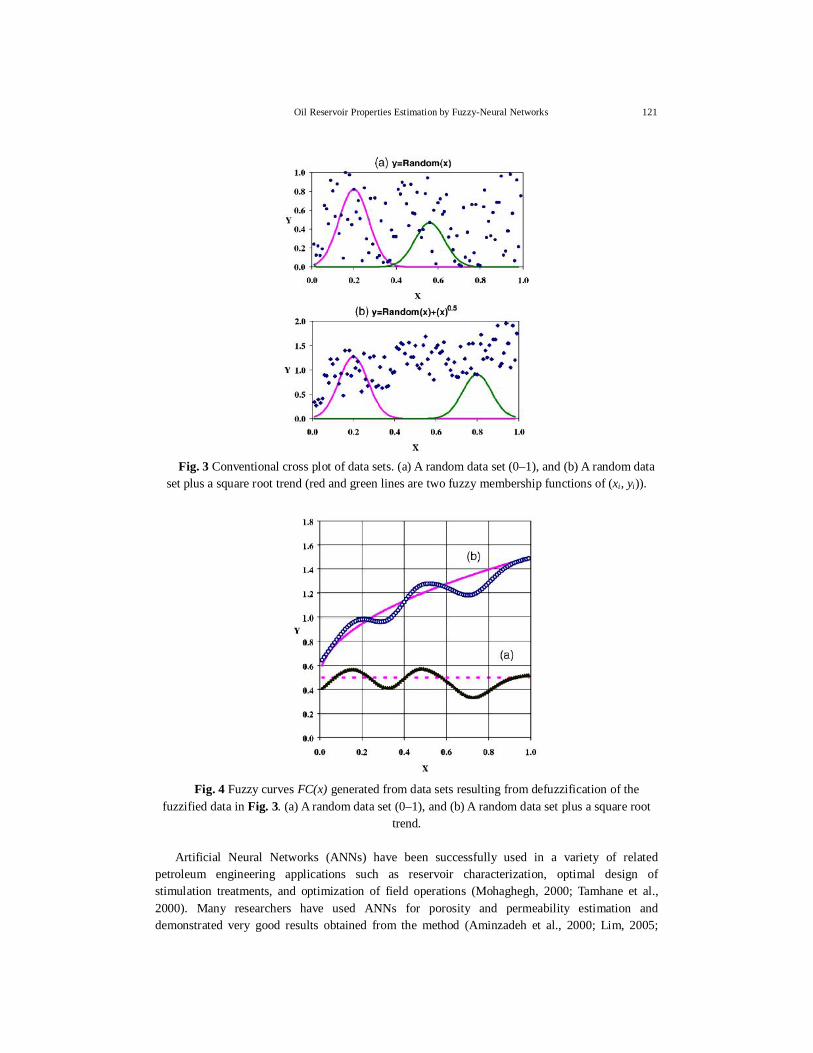
The two fuzzy curves resulting from defuzzification of the fuzzified data in Fig. 3 are shown in Fig. 4 (Weiss et al., 2001). As seen in Fig. 4, the random data set has a no-slope dashed best-fit line while the random data set plus the x0.5 trend has a best-fit line that has a range of about 0.85. The range of fuzzy curves can be used to identify related variables in noisy data sets and rank the input variables for further analysis. The selected well logs then can serve as inputs to regression or neural network to develop multivariate correlations with core measurements. Such fuzzy membership functions have been obtained with the help of a Matlab toolbox for Fuzzy logic (The MathWorks, 2000).

Ranking

Rank.1 Rank.2 Rank.3 Rank.4 Rank.5 Rank.6

Axon

Soma

Dendrite

Nucleus Myelin sheath

Schwann cell

Node of Ranvier

Axon Terminal

Neural Network

Selection best inputs for NN


Fig. 3 Conventional cross plot of data sets. (a) A random data set (0–1), and (b) A random data

set plus a square root trend (red and green lines are two fuzzy membership functions of (xi, yi)).

Fig. 4 Fuzzy curves FC(x) generated from data sets resulting from defuzzification of the

fuzzified data in Fig. 3. (a) A random data set (0–1), and (b) A random data set plus a square root trend.

Artificial Neural Networks (ANNs) have been successfully used in a variety of related

petroleum engineering applications such as reservoir characterization, optimal design of stimulation treatments, and optimization of field operations (Mohaghegh, 2000; Tamhane et al., 2000). Many researchers have used ANNs for porosity and permeability estimation and demonstrated very good results obtained from the method (Aminzadeh et al., 2000; Lim, 2005;


Aminzadeh and Brouwer, 2006). Particularly, most of the successful studies of geophysical problems used the multilayer perceptron (MLP) neural network model which is the most popular among all the existing techniques. The MLP is a variant of the original perceptron model proposed by Rosenblatt (1958) in the 1950s. The model consists of a feed-forward, layered network of McCulloch and Pitts’ neurons (McCulloch and Pitts, 1943). Each neuron in the MLP model has a nonlinear activation function that is often continuously differentiable. Some of the most frequently used activation functions for MLP model are the sigmoid and the hyperbolic tangent functions.

Basically, a neural network is composed of computer-programming objects called nodes. These nodes closely correspond in both form and function to their organic counterparts, neurons. Individually, nodes are programmed to perform a simple mathematical function, or to process a small portion of data. A node has other components, called weights, which are integral parts of the neural network. Weights are variables applied to the data that each node outputs. By adjusting a weight on a node, the data output is changed, and the behaviour of the neural network can be altered and controlled. By careful adjustment of weights, the network can learn. Networks learn their initial behaviour by being exposed to training data. The network processes the data, and a controlling algorithm adjusts each weight to arrive at the correct or final answer(s) to the data. These algorithms or procedures are called learning algorithms.

A key step in applying the MLP model is to choose the weighted matrices. Assuming a layered MLP structure, the weights feeding into each layer of neurons form a weight matrix of the layer. Values of these weights are found using the error back-propagation method. This leads to a nonlinear least square optimization problem to minimize the error. There are numerous nonlinear optimization algorithms available to solve this problem, and some of the basic algorithms are the Steepest Descend Gradient method, the Newton’s method and the Conjugate-Gradient method.

There are two separate modes in which the gradient descent algorithm can be implemented: the incremental mode and the batch mode (Battiti, 1992). In the incremental mode, the gradient is computed and the weights are updated after each input is applied to the network. In the batch mode, all the inputs are applied to the network before the weights are updated. The gradient descent algorithm with momentum converges faster than gradient descent algorithm with non-momentum. Two powerful techniques of gradient descent algorithm with momentum in incremental and batch modes are online back-propagation and batch back-propagation, respectively.

Some researches proposed high-performance algorithms that can converge from ten to one hundred times faster than conventional descend gradient algorithm, for example, the Quasi-Newton algorithm (Battiti, 1992), the Resilient Propagation algorithm - RPROP (Riedmiller and Braun, 1993), the Levenberg-Marquardt algorithm (Hagan and Menhaj, 1999) and the Quick Propagation algorithm (Ramasubramanian and Kannan, 2004). The disadvantage of the Quasi-Newton algorithm and the Levenberg-Marquardt algorithm is long training time due to complex calculations in computing the approximate of the Hessian matrix (Battiti, 1992; Hagan and Menhaj, 1999).

We have considered the mathematical basis of four training techniques, including the online back-propagation, the batch back-propagation, the RPROP and the Quick propagation algorithm, as they are the most suitable techniques. The main difference among these techniques is on the method of calculating the weights and their updating (Werbos, 1994).

The training process starts by initializing all weights with small non-zero values. Often they are generated randomly. A subset of training samples (called patterns) is then presented to the network, one at a time. A measure of the error incurred by the network is made, and the weights are updated in such a way that the error is reduced. One pass through this cycle is called an epoch. This process is repeated as required until the global minimum is reached.


In the online back-propagation algorithm, the weights are updated after each pattern is presented to the network, otherwise batch back-propagation with weight updates occurring after each epoch (Battiti, 1992). The weights are updated as follows;

1twtwtMSEtw ij

ijij

(3)

where wij is the change of the synaptic connection weight from neuron i to neuron j in the next layer, MSE is the least mean square error, is the learning rate, t is the step of training and is the momentum that pulls the network out of small local minima. And then,

wij (t+1) = wij(t) + wij(t) (4) The RPROP algorithm is an adaptive learning rate method, where weight updates are based

only on the signs of the local gradients, not their magnitudes (Riedmiller and Braun, 1993). Each weight (wij) has its own step size or update value (ij), which varies with step (t) according to the following equations;

else 1),-t(

0 )t(w

MSE 1).-t(w

MSE if 1),-t(

0)t(w

MSE 1).-t(w

MSE if 1),-t(

)t(

ij

ijijij

-

ijijij

ij

Δ

∂∂Δ

∂∂Δ

(5)

where 0<- <1<+, and the weights are updated according to:

else 0

0)t(w

Eif ),t(

0)t(w

Eif ),t(-

)t(wij

ij

ijij

ijMS ∂Δ

MS ∂Δ

Δ (6)

The Quick propagation is a training method based on the following assumptions (Ramasubramanian and Kannan, 2004):

1. MSE(w) for each weight can be approximated by a parabola that opens upward, and 2. The change in slope of MSE(w) for this weight is not affected by all other weights that

change at the same time. The weights update rule is

)t(Q)1t(w)t(Q)1t(Q

)t(Qtw ijij

(7)

where Q(t)=MSE/wij(t) is the derivative of the error with respect to the weight and {Q(t-1)-Q(t)}/wij(t-1) is its finite difference approximation. Together these approximate, Newton’s method for minimizing a one-dimensional function f(x) is applied as x=-f’(x)/f ’’(x).

In general, too low learning rate makes the network learning very slowly, whereas too high learning rate makes the weights and error function diverge, so there is no learning at all. In this view, we used fixed values of 0.1 and 0.5 for the learning rate () and the momentum (), respectively. Although using these relatively low values may be time-consuming, they give accurate results.


The activation function (a) used at each hidden layer and the output layer is logistic, and that is a sigmoid function with smooth step. This is expressed by

ue11a

(8)

where u is the output of any neuron in the network (or net function). The derivative of this function has a Gaussian shape, which helps to stabilize the network and to compensate for overcorrection of the weights.

In this study, many paradigms have been tried to find out the most efficient one. And we found that batch back-propagation and quick propagation are two most successful paradigms for the porosity/permeability estimation problem; the difference of the two paradigms is the method of calculating the weights and their updates using Equations (3) and (7).

3. Training and Testing of Fuzzy-Neural Networks

3.1 Training data set 3.1.1 Well log data

A well log is a record of characteristics of the formation traversed by a measurement in the well bore. It provides a means to evaluate the formation characteristics and the hydrocarbon production potential of a reservoir. Logging tools can be grouped into two categories: conventional and unconventional well logs. Conventional well logs are those that are routinely collected at almost all industry boreholes. Unconventional well logs are either too specialized, expensive or too recently developed to be run in every well. For input of training data in this study, we consider eight well log curves which are measured most fully in the A2-VD prospect, that are caliper, sonic, gamma ray, laterlog deep - LLD, laterlog shallow - LLS, microspherically focused log - MSFL, neutron and density logs (Fig. 5).

3.1.2 Core samples data

Core analysis is the process of obtaining information about the properties of the subsurface by the examination of core samples taken from a borehole during drilling. The set of measurements carried out on cores of this study includes porosity and permeability. Core analysis is one of the techniques used for identification and characterization of natural fractures. It can provide quantification of fracture geometry, fracture frequency and the nature of any filling material. Among the disadvantages of core analysis for naturally fractured reservoirs evaluation are:

- It is difficult to assess how representative the core plug is of the reservoir. - Cores that contain fractures of practical significance are often lost in the process of

recovery. - Mechanical fractures are often induced on the cores during the recovery process as a result

of retrieving the core and stress release as the core is brought to the surface. - Core analysis is costly, labor intensive, and subject to the availability of drilled rocks. These factors have directed the industry to employ well logs that are cost-effective and readily

available. Among the advantages of well logs over core analysis are: - Typically cores are obtained over a small portion of the well. Well logs are run over a

significantly larger portion. - Well logs provide in-situ measurements of the formation at reservoir conditions. - Well logs provide a consistent one-dimensional profile of rock properties expressed in terms

of a consistent length scale. Because they are highly affected by the borehole condition, noise needs to be rejected noise before


interpretation. In the A2-VD prospect, cored intervals are short (<5 m) and the recovery is no more than 67% reflecting the high intensity of fracturing in the reservoir. All recovered cores are broken into small pieces, the longest continuous pieces are 30 cm to 50 cm long and come from non-fractured intervals (Hung and Hung, 2004).

Within the core, the preserved fractures are moderately (45° to 70°) to steeply (80° to 90°) dipping with variable widths ranging from < 0.5mm to 3cm. Fractures dipping 45° to 60° are dominant with occasional caverns in their central portions. Most fractures are filled with secondary silica, zeolites, and/or calcite cements. Drilling-induced and exfoliation fractures are also present, at depth, where only the exfoliation fractures are effective in term of lateral drainage. Normally, cores can be oriented using FMI/FMS imaging, but this requires continuous lengths of core with suitable anisotropic features. The recovered cores are always broken, due to the intersection of major fractures; therefore it was not possible to orient the cores using FMI/ FMS. Consequently, the orientation of fractures in cores could not be determined.

In this study, among the recovery cores (67%), we selected 97 good samples for well-representative of fractured porosity and 98 good samples for well-representative of permeability. These core samples were collected at intervals of 3100-3400 meters and 3800-4000 meters at 7 wells of the A2-VD prospect. The core samples measurements were used for output of the training data set (Fig. 5). The fractured porosity in the prospect is defined as interconnected pore volumes of macrofractures, microfractures and vugs. Although core samples selected in this work mainly at intervals with presenting of microfractures and vugs, but they can be used for training a neural network which can predict fractured porosity from well log data.

- Macrofractures Macrofractures are mainly formed by tectonic activities and consist of two intersected systems

creating angles varied from 40o to 120o. Radius of filtrate invasions in macrofracture zones is principally affected by the pressure difference between mud column in the borehole and formation, in another word, it depends on hydrodynamic energies. Macrofracture zones can be observed on both seismic profiles and CAST-V data, their thickness varies from some meters to 60 meters. However, macrofracture zone thickness is dominant in a range of 2-4 meters. Spaces between macrofracture zones of the fractured basement vary from some meters to 100 meters, even some hundred meters.

- Microfractures Microfractures distribute along surfaces of macrofractures. In microfracture rocks, mud filtrate

invasion is resulted mainly from capillary pressure. Utilization of log data to identify microfracture zones is very difficult. In some cases, these zones might be identified by slight increase of DT and NPHI values.

- Secondary vugs Secondary vug systems were formed and developed mainly along surfaces of macrofractures.

The presence of secondary vugs improves significantly the storage capacity of the basement reservoirs.


500

1000

1500

2000

2500

3000

3500

Dep

th (m

)

500

1000

1500

2000

2500

3000

3500

500

1000

1500

2 000

2500

3000

3500

500

1000

1500

2000

2500

3000

3500

Dep

th (m

)

500

1000

1500

2000

2500

3000

3500

500

1000

1500

2000

2500

3000

3500

0 10 15 20 25 50 100 150 200 0 50 100 150 200 250

Caliper DTCO (ms/ft)

GR (gamma)

LLD (Ohmm)

LLS (Ohmm)

MSFL (Ohmm)

0.1 101 105 0.1 101 105 0.1 101 105

NPHI (%)

RHOB (g/cc)

0 0. 1 0.2 0.3 0.4 1 1.5 2 2 .5 3

3500

3000

2500

2000

1500

1000

500

3500

3000

2500

2000

1500

1000

500

Dep

th (m

)

(a) Well log data used as input data for NN

(b) Core samples from which the output of NN is

given

Fig. 5 Training data set.


3.2 Fuzzy ranking In the A2-VD prospect, because of complex well bore conditions in basement rock, significant

noises of log data are present. Therefore, a fuzzy ranking has been used for selecting the best related well logs with core porosity and permeability data. Then, ANNs is used as a nonlinear regression method to develop transformation between the selected well logs and core measurements.

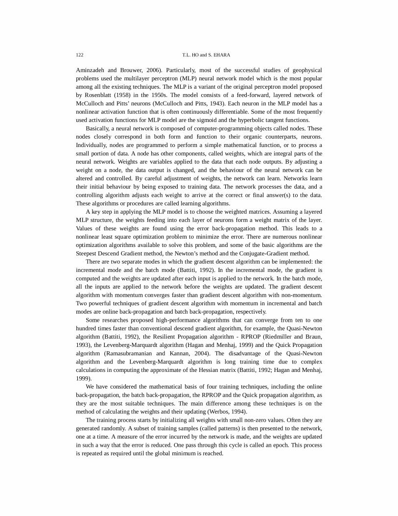
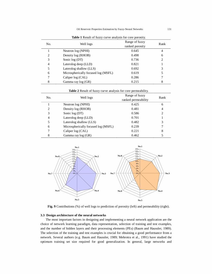
The first step is to determine the strength of the relationships between the variables. We constructed the cross plots between well logs and core measurements, but found weak correlation based on correlation coefficients and visual observations (Figs. 6 and 7). Next, fuzzy curve analysis based on fuzzy logic was utilized to analyse correlation between the variables. Normalized data by the maximum-minimum normalization equation were used for fuzzy curves generation. Figure 8 shows the fuzzy ranked porosity and permeability curves for each well log. These fuzzy curves could identify visual relationship between core measurements and well logs from noisy data sets. Fuzzy curve analysis could help to select the best related well log with core analysis data as input for regressions and neural networks. The ranges of fuzzy ranked curves were used as the ranking criteria. The results of analyzing porosity and permeability fuzzy curves are tabulated in Tables 1 and 2, respectively. We selected six well logs (NPHI, RHOB, DT, LLD, LLS and MSFL) for porosity estimation. NPHI, RHOB, DT, LLD, LLS and GR were chosen for permeability model. The contributions of each well log to prediction of porosity and permeability are shown in Fig. 9.


Neutron Log

0.00

0.10

0.20

0.30

0.40

0.00 0.02 0.04 0.06 0.08 0.10 0.12

Core porosity

Neu

tron

Log

(%)

Sonic Log

5060708090

100110120

0.00 0.02 0.04 0.06 0.08 0.10 0.12

Core porosity

Soni

cLo

g(m

s/ft)

Gamma Ray Log

50

70

90

110

130

150

0.00 0.02 0.04 0.06 0.08 0.10 0.12

Core porosity

Gam

ma

Ray

Log

(gam

ma)

Caliper Log

5

8

11

14

17

20

0.00 0.02 0.04 0.06 0.08 0.10 0.12

Core porosity

Cal

iper

Log

(inch

)

Density Log

1.0

1.5

2.0

2.5

3.0

0.00 0.02 0.04 0.06 0.08 0.10 0.12

Core porosity

Den

sity

Log

(g/c

c)

Laterolog Deep Log

100

1000

10000

100000

0.00 0.02 0.04 0.06 0.08 0.10 0.12

Core porosity

Late

rolo

gD

eep

Log

(Ohm

.m)

Laterolog Shallow Log

100

1000

10000

100000

0.00 0.02 0.04 0.06 0.08 0.10 0.12

Core porosity

Late

rolo

gSh

allo

wLo

g(O

hm.m

)

Microspherically focused Log

10

100

1000

10000

0.00 0.02 0.04 0.06 0.08 0.10 0.12

Core porosity

Mic

rosp

heric

ally

focu

sed

Log

(Ohm

.m)

Fig. 6 Scatter plots of core porosity and well logs.


Neutron Log

0.00

0.10

0.20

0.30

0.40

0 200 400 600 800 1000

Core permeability (md)

Neu

tron

Log

(%)

Sonic Log

5060708090

100110120

0 200 400 600 800 1000


Soni

cLo

g(m

s/ft)

Gamma Ray Log

50

70

90

110

130

150

0 200 400 600 800 1000


Gam

ma

Ray

Log

(gam

ma)

Caliper Log

5

8

11

14

17

20

0 200 400 600 800 1000


Cal

iper

Log

(inch

)

DensityLog

1.0

1.5

2.0

2.5

3.0

0 200 400 600 800 1000


Den

sity

Log

(g/c

c)

Laterolog Deep Log

100

1000

10000

100000

0 200 400 600 800 1000


Late

rolo

gD

eep

Log

(Ohm

.m)


100

1000

10000

100000

0 200 400 600 800 1000


Late

rolo

gSh

allo

wLo

g(O

hm.m

)


10

100

1000

10000

0 200 400 600 800 1000


Mic

rosp

heric

ally

focu

sed

Log

(Ohm

.m)

Fig. 7 Scatter plots of core permeability and well logs.


Neutron Log

0.0

0.2

0.4

0.6

0.8

1.0

0.0 0.2 0.4 0.6 0.8 1.0

Neutron Log

Fuzz

yR

anke

dVa

lue

porositypermeability

Density Log

0.0

0.2

0.4

0.6

0.8

1.0

0.0 0.2 0.4 0.6 0.8 1.0

Density Log

Fuzz

yR

anke

dVa

lue


Gamma Ray Log

0.0

0.2

0.4

0.6

0.8

1.0

0.0 0.2 0.4 0.6 0.8 1.0

Gamma Ray Log

Fuzz

yR

anke

dVa

lue


Sonic Log

0.0

0.2

0.4

0.6

0.8

1.0

0.0 0.2 0.4 0.6 0.8 1.0

Sonic Log

Fuzz

yR

anke

dVa

lue


Laterolog Dee p Log

0.0

0.2

0.4

0.6

0.8

1.0

0.0 0 .2 0.4 0.6 0.8 1 .0

Laterolog Deep Log

Fuzz

yRa

nked

Valu

e



0.0

0.2

0.4

0.6

0.8

1.0

0.0 0.2 0.4 0.6 0.8 1.0


Fuzz

yR

anke

dVa

lue



0.0

0.2

0.4

0.6

0.8

1.0

0.0 0.2 0.4 0.6 0.8 1.0


Fuzz

yR

anke

dLo

g


Caliper Log

0.0

0.2

0.4

0.6

0.8

1.0

0.0 0.2 0.4 0.6 0.8 1.0

Caliper Log

Fuzz

yR

anke

dVa

lue


Fig. 8 Fuzzy ranked porosity and permeability curves for well logs.


Table 1 Result of fuzzy curve analysis for core porosity.

No. Well logs Range of fuzzy ranked porosity

Rank

1 2 3 4 5 6 7 8

Neutron log (NPHI) Density log (RHOB) Sonic log (DT) Laterolog deep (LLD) Laterolog shallow (LLS) Microspherically focused log (MSFL) Caliper log (CAL) Gamma ray log (GR)

0.645 0.498 0.736 0.821 0.692 0.619 0.286 0.215

4 6 2 1 3 5 7 8

Table 2 Result of fuzzy curve analysis for core permeability.

No. Well logs Range of fuzzy

ranked permeability Rank

1 2 3 4 5 6 7 8

Neutron log (NPHI) Density log (RHOB) Sonic log (DT) Laterolog deep (LLD) Laterolog shallow (LLS) Microspherically focused log (MSFL) Caliper log (CAL) Gamma ray log (GR)

0.425 0.481 0.586 0.701 0.482 0.239 0.221 0.462

6 4 2 1 3 7 8 5

0%2%4%6%8%

10%12%14%16%18%20%

No.1

No.2

No.3

No.4

No.5

No.6

No.7

No.8

0%2%4%6%8%

10%12%14%16%18%20%

No.1

No.2

No.3

No.4

No.5

No.6

No.7

No.8

Fig. 9 Contributions (%) of well logs to prediction of porosity (left) and permeability (right). 3.3 Design architecture of the neural networks

The most important factors in designing and implementing a neural network application are the choice of network learning paradigm, data representation, selection of training and test examples, and the number of hidden layers and their processing elements (PEs) (Baum and Haussler, 1989). The selection of the training and test examples is crucial for obtaining a good performance from a network. Several authors (e.g. Baum and Haussler, 1989; Mehrotra et al., 1991) have studied the optimum training set size required for good generalization. In general, large networks and


complicated input patterns require more training examples for an optimum generalization (Kung and Hwang, 1988; Rajavelu et al., 1989). In this study we have designed and implemented two kinds of networks for training and testing of porosity network and permeability network. In both of porosity and permeability networks training cases, it was found that a three-layer network is the most effective.

The architecture of these networks was used as shown in Fig. 10 with one input layer composed of six nodes. These six nodes represent the response of neutron, density, sonic, resistivity (LLS, LLD and MSFL) in porosity network and neutron, density, sonic, gamma ray, resistivity (LLS, LLD) in permeability network. A single hidden layer has five nodes and the output layer has only one node that representing porosity or permeability. With data of this study area, more hidden layers or more neurons of each layer is ineffective and increase unnecessary complex calculations.

The sources of training data for the porosity and permeability networks were selected from well logs data and core samples in corresponding depths of those logs (Fig. 5). We implemented batch back-propagation algorithm for porosity network training, while quick propagation algorithm is more effective in the training case of permeability network.

Fig. 10 Block diagrams of the back propagation neural network.

3.4 Training and testing

Figure 11(a) shows the RMS error as a function of iteration number during training of porosity data set. The error begins high and decreases as the iteration proceeds until it attains an almost

Density

NPHI

Sonic

LLS

GR

LLD

PPeerrmmeeaabbiill iittyy

Hidden layer

Output layer

Connection

weights

(PEs)

Density

NPHI

Sonic

LLS

MSFL

LLD

PPoorroossiittyy

Hidden layer

Output layer

Connection

weights

(PEs)

Input layer Input layer


constant value of about 0.02 after 6291 iterations, hence the network attains convergence. Once the network attains convergence, the weights are adapted and stored in a weight file. Using these adapted weights, the network determines porosity from well logs directly in a few seconds without any more training.

Figure 11(b) shows the RMS error as a function of iteration number during training of permeability data set. In the data set of permeability, the core data are rougher than porosity due to more sensitiveness of permeability in fracture intervals and non-fracture intervals alternately. That is the reason why the error starts off quite high, about 58, but it also decreases continuously to 0.1 after 800 iterations. The convergence of error is attained after 1143 iterations with an error of 0.05.

The networks were trained by trial-and-error for each data representation to produce the lowest errors. In back-propagation, too low learning rate makes the network learning very slow, while an excessively high learning rate makes the weights and error function diverge, so there is no learning at all. In view of this, fixed values of 0.1 and 0.5 were used for the learning rate () and the momentum (), respectively. Although using these relatively low values may be time-consuming, they give accurate results. For training of networks, we used data set from core samples of 70 patterns for porosity NN and 65 patterns for permeability NN. The porosity and permeability networks performance were tested using 27 patterns and 33 patterns testing sets, respectively (Fig. 12).

RMS Error vs Training Time

00.010.020.030.040.050.060.070.080.090.1

0 500 1000 1500 2000 2500 3000 3500 4000 4500 5000 5500 6000 6500 7000Epochs

RM

S E

rror

Traning Error

RMS Error vs Training Time

05

101520253035404550556065

0 100 200 300 400 500 600 700 800 900 1000 1100 1200 1300

Epochs

RM

S E

rror

Traning Error

Fig. 11 RMS errors as a function of iteration number during training of (a) Porosity and (b) Permeability data sets.

(a)

(b)


0.02

0.04

0.07

0.09

0.00

0.11

0.001 9 17 25 33 41 49 57 65 70

Pattern #

Erro

r

Trai

ning

Dat

a

RMS Error Vs. Patternfor all Nodes

0.02

0.04

0.07

0.09

0.00

0.11

0.001 5 9 13 17 21 25 27

Pattern #

Erro

r

Test

ing

Dat

a


0.02

0.04

0.07

0.09

0.00

0.11

0.001 9 17 25 33 41 49 57 65

Pattern #

Erro

r

Trai

ning

Dat

a


0.02

0.04

0.06

0.08

0.00

0.10

0.001 5 9 13 17 21 25 29 33

Pattern #

Erro

r

Test

ing

Dat

a


Fig. 12 RMS errors as a function of training and testing data set patterns of (a) porosity network, and (b) permeability network.

(a)

(b)


4. Fuzzy-Neural Networks Results For a comparative study, both empirical porosity/permeability prediction method (so called

LOG porosity/permeability) and neural networks (so called ANN porosity/permeability) were applied to the selected well log data and the computed results were compared with core measured porosity and permeability.

In the A2-VD prospect, the fractured porosity is calculated by the following equation (JVPC report, 2001):

)3(R23

R32

R1

frtbl

fr

mf

fr

tfr

, (9)

where Rtfr, Rtbl and Rmf - resistivity of fracture reservoir, block and mud filtrate, respectively. The value of the resistivity gradient has been used to estimate the order of magnitude of

formation permeability by Schlumberger log interpretation chart. The chart uses the following equation:

,R1*

DRc

,3.2*cTk

0

2

hw

(10)

where T is a constant, normally about 20, R is the change in resistivity (ohm-m), D is the change in depth corresponding to R (ft), R0 is the 100% water-saturated formation resistivity (ohm-m), w is formation water density (g/cm3), and h is hydrocarbon density (g/cm3).

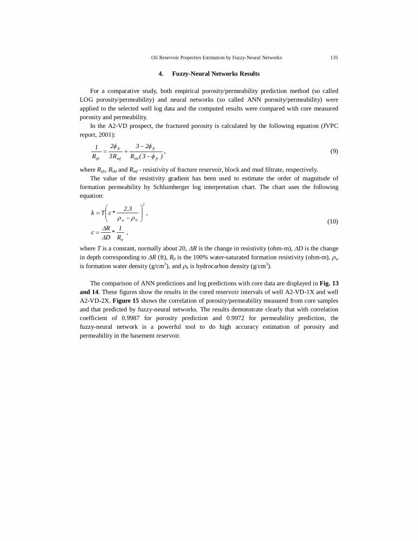
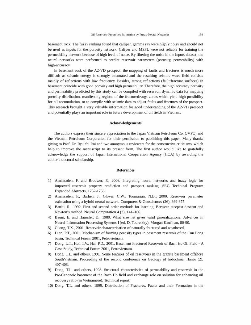
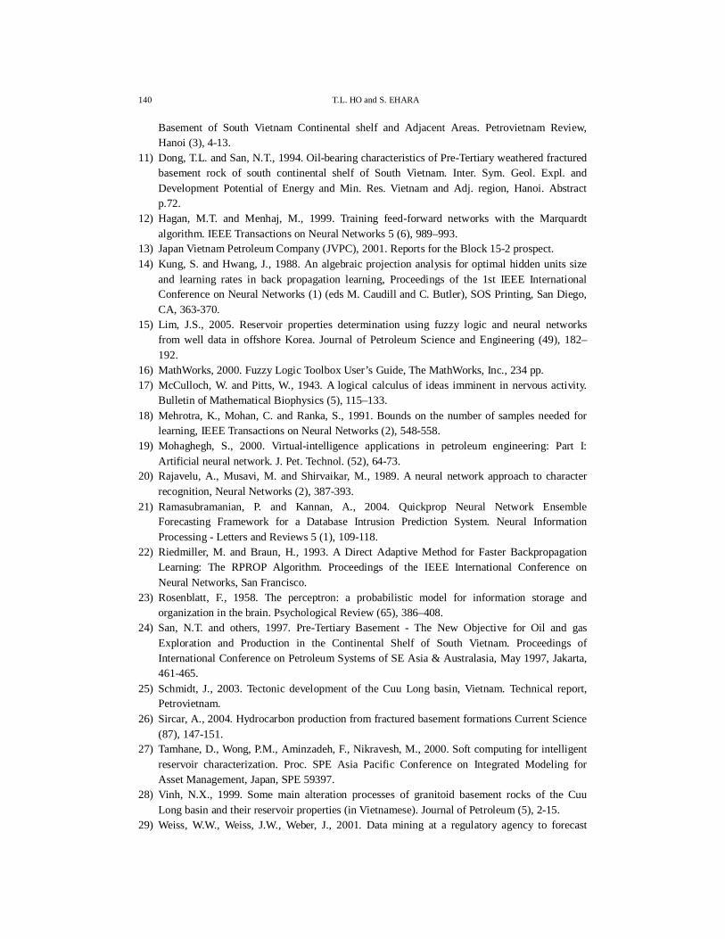
The comparison of ANN predictions and log predictions with core data are displayed in Fig. 13

and 14. These figures show the results in the cored reservoir intervals of well A2-VD-1X and well A2-VD-2X. Figure 15 shows the correlation of porosity/permeability measured from core samples and that predicted by fuzzy-neural networks. The results demonstrate clearly that with correlation coefficient of 0.9987 for porosity prediction and 0.9972 for permeability prediction, the fuzzy-neural network is a powerful tool to do high accuracy estimation of porosity and permeability in the basement reservoir.


(a)

0.03

0.04

0.05

0.06

0.07

3218 3220 3222 3224 3226 3228 3230 3232 3234 3236 3238 3240

depth (m)

poro

sity Core porosity

ANN porosityLOG porosity

(b)

0.03

0.04

0.05

0.06

0.07

3165 3170 3175 3180 3185 3190 3195 3200 3205 3210

depth (m)

poro

sity Core porosity

ANN porosityLOG porosity

Fig. 13 Comparison of porosity predicted by ANN and practical method to that of core samples

in (a) Well A2-VD-1X, (b) Well A2-VD-2X.


(a)

35

40

45

50

55

3960 3961 3962 3963 3964 3965 3966 3967 3968 3969 3970 3971 3972

depth (m)

perm

eabi

lity

(md)

Core permeabilityANN permeabilityLOG permeability

(b)

70

75

80

85

90

95

100

105

3875 3880 3885 3890 3895 3900 3905 3910 3915 3920 3925

depth (m)

perm

eabi

lity

(md)

Core permeabilityANN permeabilityLOG permeability

Fig. 14 Comparison of permeability predicted by ANN and practical method to that of core samples in (a) Well A2-VD-1X, (b) Well A2-VD-2X.


R2 = 0.9987

0

0.02

0.04

0.06

0.08

0.1

0.12

0 0.02 0.04 0.06 0.08 0.1 0.12

Core porosity

AN

N p

oros

ity

R2 = 0.9972

0

200

400

600

800

1000

0 200 400 600 800 1000

Core permeability

AN

N p

erm

eabi

lity

Fig. 15 Porosity and permeability correlation between core samples and neural networks

prediction.

5. Conclusions Because of the small number compared with clastic and carbonate reservoirs, the basement

reservoirs were named un-usual reservoir and has become an attractive target and has been paid a great attention for investigation. In this paper, we introduced an efficient method for the basement reservoir properties estimation using fuzzy-neural networks.

After many trials of various algorithms, a three-layered feed-forward neural network using the Batch Back-Propagation learning algorithm was chosen for porosity network. Meanwhile the Quick Propagation learning algorithm was more effective for permeability network. For the small size training data set, the architectures of the networks were selected based on heuristic method. Input of these networks was well log data sets. Eight logging curves had been used which are gamma ray, calliper, neutron, density, sonic and three resistivity logs (LLS, LLD, MSFL). A fuzzy ranking technique has been deployed to identify noise of well log data by correlation with core measurements. The noise probably occurred due to complex borehole condition in fractured/vugs


basement rock. The fuzzy ranking found that calliper, gamma ray were highly noisy and should not be used as inputs for the porosity network. Caliper and MSFL were not reliable for training the permeability network because of high level of noise. By filtering the noise in the inputs dataset, the neural networks were performed to predict reservoir parameters (porosity, permeability) with high-accuracy.

In basement rock of the A2-VD prospect, the mapping of faults and fractures is much more difficult as seismic energy is strongly attenuated and the resulting seismic wave field consists mainly of reflections with low frequency. Besides, strong reflections (fault/fracture surfaces) in basement coincide with good porosity and high permeability. Therefore, the high accuracy porosity and permeability predicted by this study can be compiled with reservoir dynamic data for mapping porosity distribution, manifesting regions of the fractured/vugs zones which yield high possibility for oil accumulation, or to compile with seismic data to adjust faults and fractures of the prospect. This research brought a very valuable information for good understanding of the A2-VD prospect and potentially plays an important role in future development of oil fields in Vietnam.

Acknowledgements

The authors express their sincere appreciation to the Japan Vietnam Petroleum Co. (JVPC) and

the Vietnam Petroleum Corporation for their permission to publishing this paper. Many thanks giving to Prof. Dr. Ryuichi Itoi and two anonymous reviewers for the constructive criticisms, which help to improve the manuscript to its present form. The first author would like to gratefully acknowledge the support of Japan International Cooperation Agency (JICA) by awarding the author a doctoral scholarship.

References 1) Aminzadeh, F. and Brouwer, F., 2006. Integrating neural networks and fuzzy logic for

improved reservoir property prediction and prospect ranking, SEG Technical Program Expanded Abstracts, 1752-1756.

2) Aminzadeh, F., Barhen, J., Glover, C.W., Toomarian, N.B., 2000. Reservoir parameter estimation using a hybrid neural network. Computers & Geosciences (26), 869-875.

3) Battiti, R., 1992. First and second order methods for learning: Between steepest descent and Newton’s method. Neural Computation 4 (2), 141–166.

4) Baum, E. and Haussler, D., 1989. What size net gives valid generalization?, Advances in Neural Information Processing Systems I (ed. D. Touretzky), Morgan Kaufman, 80-90.

5) Cuong, T.X., 2001. Reservoir characterisation of naturally fractured and weathered. 6) Dien, P.T., 2001. Mechanism of forming porosity types in basement reservoir of the Cuu Long

basin, Technical Forum 2001, Petrovietnam. 7) Dong, L.T., Hoi, T.V., Hai, P.D., 2001. Basement Fractured Reservoir of Bach Ho Oil Field - A

Case Study, Technical Forum 2001, Petrovietnam. 8) Dong, T.L. and others, 1991. Some features of oil reservoirs in the granite basement offshore

SouthVietnam. Proceeding of the second conference on Geology of Indochina, Hanoi (2), 407-408.

9) Dong, T.L. and others, 1998. Structural characteristics of permeability and reservoir in the Pre-Cenozoic basement of the Bach Ho field and exchange role on solution for enhancing oil recovery ratio (in Vietnamese). Technical report.

10) Dong, T.L. and others, 1999. Distribution of Fractures, Faults and their Formation in the


Basement of South Vietnam Continental shelf and Adjacent Areas. Petrovietnam Review, Hanoi (3), 4-13.

11) Dong, T.L. and San, N.T., 1994. Oil-bearing characteristics of Pre-Tertiary weathered fractured basement rock of south continental shelf of South Vietnam. Inter. Sym. Geol. Expl. and Development Potential of Energy and Min. Res. Vietnam and Adj. region, Hanoi. Abstract p.72.

12) Hagan, M.T. and Menhaj, M., 1999. Training feed-forward networks with the Marquardt algorithm. IEEE Transactions on Neural Networks 5 (6), 989–993.

13) Japan Vietnam Petroleum Company (JVPC), 2001. Reports for the Block 15-2 prospect. 14) Kung, S. and Hwang, J., 1988. An algebraic projection analysis for optimal hidden units size

and learning rates in back propagation learning, Proceedings of the 1st IEEE International Conference on Neural Networks (1) (eds M. Caudill and C. Butler), SOS Printing, San Diego, CA, 363-370.

15) Lim, J.S., 2005. Reservoir properties determination using fuzzy logic and neural networks from well data in offshore Korea. Journal of Petroleum Science and Engineering (49), 182– 192.

16) MathWorks, 2000. Fuzzy Logic Toolbox User’s Guide, The MathWorks, Inc., 234 pp. 17) McCulloch, W. and Pitts, W., 1943. A logical calculus of ideas imminent in nervous activity.

Bulletin of Mathematical Biophysics (5), 115–133. 18) Mehrotra, K., Mohan, C. and Ranka, S., 1991. Bounds on the number of samples needed for

learning, IEEE Transactions on Neural Networks (2), 548-558. 19) Mohaghegh, S., 2000. Virtual-intelligence applications in petroleum engineering: Part I:

Artificial neural network. J. Pet. Technol. (52), 64-73. 20) Rajavelu, A., Musavi, M. and Shirvaikar, M., 1989. A neural network approach to character

recognition, Neural Networks (2), 387-393. 21) Ramasubramanian, P. and Kannan, A., 2004. Quickprop Neural Network Ensemble

Forecasting Framework for a Database Intrusion Prediction System. Neural Information Processing - Letters and Reviews 5 (1), 109-118.

22) Riedmiller, M. and Braun, H., 1993. A Direct Adaptive Method for Faster Backpropagation Learning: The RPROP Algorithm. Proceedings of the IEEE International Conference on Neural Networks, San Francisco.

23) Rosenblatt, F., 1958. The perceptron: a probabilistic model for information storage and organization in the brain. Psychological Review (65), 386–408.

24) San, N.T. and others, 1997. Pre-Tertiary Basement - The New Objective for Oil and gas Exploration and Production in the Continental Shelf of South Vietnam. Proceedings of International Conference on Petroleum Systems of SE Asia & Australasia, May 1997, Jakarta, 461-465.

25) Schmidt, J., 2003. Tectonic development of the Cuu Long basin, Vietnam. Technical report, Petrovietnam.

26) Sircar, A., 2004. Hydrocarbon production from fractured basement formations Current Science (87), 147-151.

27) Tamhane, D., Wong, P.M., Aminzadeh, F., Nikravesh, M., 2000. Soft computing for intelligent reservoir characterization. Proc. SPE Asia Pacific Conference on Integrated Modeling for Asset Management, Japan, SPE 59397.

28) Vinh, N.X., 1999. Some main alteration processes of granitoid basement rocks of the Cuu Long basin and their reservoir properties (in Vietnamese). Journal of Petroleum (5), 2-15.

29) Weiss, W.W., Weiss, J.W., Weber, J., 2001. Data mining at a regulatory agency to forecast


water flood recovery. Proc. SPE Rocky Mountain Petroleum Technology Conference, Keystone, Colorado, SPE 71057.

30) Werbos, P.J., 1994. The Roots of Back-Propagation. John Wiley & Sons, Inc. 31) Zadeh, L.A., 1988. Fuzzy Logic, IEEE Computer, 83-89.

oil reservoir properties estimation by fuzzy-neural...

Documents