okun's law: fit at 50? - johns hopkins university

LAURENCE BALL

DANIEL LEIGH

PRAKASH LOUNGANI

Okun’s Law: Fit at 50?

This paper asks how well Okun’s Law fits short-run unemployment move-ments in the United States since 1948 and in 20 advanced economies since1980. We find that Okun’s Law is a strong relationship in most countries, andone that is fairly stable over time. Accounts of breakdowns in the Law, suchas the emergence of “jobless recoveries,” are flawed or exaggerated. Wealso find that the coefficient in the relationship—the effect of a 1% changein output on the unemployment rate—varies substantially across countries.This variation is partly explained by idiosyncratic features of national la-bor markets, but it is not related to differences in employment protectionlegislation.

JEL codes: E24, E32Keywords: unemployment, Okun’s Law, economic fluctuations.

IN 1962, ARTHUR OKUN REPORTED AN EMPIRICAL REGULARITY:a negative short-run relationship between unemployment and output. Many studieshave confirmed this finding, and Okun’s Law has become a fixture in macroeconomicstextbooks. For the United States, many authors posit that a 1% deviation of outputfrom potential causes an opposite change in unemployment of half a percentage point(e.g., Mankiw 2012).

Yet many economists question Okun’s Law. A number of recent papers have titleslike “The Demise of Okun’s Law” (Gordon 2010) and “An Unstable Okun’s Law,

We thank the editor and two referees for very useful comments. We are also grateful to Paul Beaudry,Olivier Blanchard, Dan Citrin, Mai Chi Dao, Davide Furceri, Michael Goldby, Pierre-Olivier Gourinchas,Juan Jimeno, Ayhan Kose, Akito Matsumoto, and seminar participants at the 2012 IMF Annual ResearchConference for helpful comments and suggestions. Jair Rodriguez and Nathalie Gonzalez Prieto providedexcellent research assistance. The views expressed in this paper are those of the authors and do notnecessarily represent those of the IMF or IMF policy.

LAURENCE BALL is a Professor at the Economics Department, Johns Hopkins University (E-mail:[email protected]). DANIEL LEIGH is a Deputy Division Chief at the Western Hemisphere Department, Inter-national Monetary Fund (E-mail: [email protected]). PRAKASH LOUNGANI is a Division Chief at ResearchDepartment, International Monetary Fund (E-mail: [email protected]).

Received June 3, 2013; and accepted in revised form February 16, 2017.

Journal of Money, Credit and Banking, Vol. 49, No. 7 (October 2017)C© 2017 The Ohio State University

1414 : MONEY, CREDIT AND BANKING

Not the Best Rule of Thumb” (Meyer and Tasci 2012). Observers have suggested thateach of the last three U.S. recessions was followed by a “jobless recovery” in whichemployment growth was weaker than Okun’s Law predicts. Studies of internationaldata suggest that Okun’s Law is unstable in many countries (e.g., Cazes, Verick,and Al-Hussami 2011). Some find that the relationship broke down during the GreatRecession of 2008–2009, when there was little correlation across countries betweenthe changes in output and unemployment (e.g., IMF 2010).

These claims matter for the interpretation of unemployment movements and formacropolicy. Okun’s Law is a part of textbook models in which shifts in aggregatedemand cause changes in output, which, in turn, lead firms to hire and fire workers. Inthese models, when unemployment is high, it can be reduced through demand stim-ulus. Skeptics of Okun’s Law question this policy view. McKinsey Global Institute(2011), for example, argues that Okun’s Law has broken down because of problemsin the labor market, such as mismatch between workers and jobs. They stress labormarket policies such as job training, not demand stimulus, as the key to reducingunemployment.

This paper asks how well Okun’s Law explains short-run unemployment move-ments. We examine data for the United States since 1948 and for 20 advancedcountries since 1980. Our principal conclusions are that Okun’s Law is a strongrelationship in most countries, and one that is fairly stable over time. We find somedeviations from a fixed Okun’s Law, but they are usually modest in size. Overall, thedata are consistent with traditional models in which fluctuations in unemploymentare caused by shifts in aggregate demand.

There is one major qualification to the universality of Okun’s Law. While thisrelationship fits the data in most countries, the coefficient in the relationship—theeffect of a 1% change in output on the unemployment rate—varies quite a bit acrosscountries. We estimate, for example, that the coefficient is –0.17 in Japan, –0.48in the United States, and –0.82 in Spain. These differences reflect special featuresof national labor markets, such as Japan’s tradition of lifetime employment and theprevalence of temporary employment contracts in Spain.

Section 1 of this paper introduces Okun’s Law and alternative approaches toestimating it. The rest of the paper demonstrates the good fit of the relation-ship and points out common flaws in analyses that report breakdowns of thelaw.

Section 2 examines U.S. annual and quarterly data over the period 1948–2013.Simple linear versions of Okun’s Law produce coefficients of –0.4 or –0.5, with R2sin the neighborhood of 0.8. We find statistical evidence of some nonlinearity andinstability in the law, but allowing for these factors does not greatly improve its fit tothe data.

Section 3 examines the common claim that U.S. recoveries since the 1990s havebeen “jobless.” We find little evidence that Okun’s Law broke down during theseepisodes. Confusion on this issue has arisen because output grew more slowly in recentrecoveries than in earlier ones, leading to disappointing outcomes for employment.(Galı, Smets, and Wouters 2012 make a similar point.)

LAURENCE BALL, DANIEL LEIGH, AND PRAKASH LOUNGANI : 1415

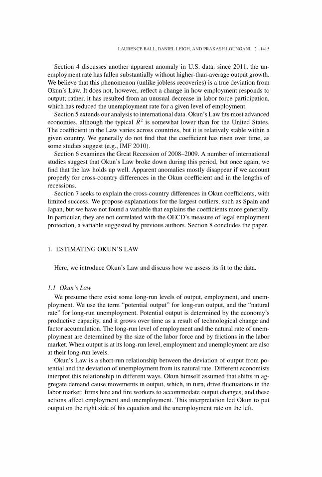
Section 4 discusses another apparent anomaly in U.S. data: since 2011, the un-employment rate has fallen substantially without higher-than-average output growth.We believe that this phenomenon (unlike jobless recoveries) is a true deviation fromOkun’s Law. It does not, however, reflect a change in how employment responds tooutput; rather, it has resulted from an unusual decrease in labor force participation,which has reduced the unemployment rate for a given level of employment.

Section 5 extends our analysis to international data. Okun’s Law fits most advancedeconomies, although the typical R2 is somewhat lower than for the United States.The coefficient in the Law varies across countries, but it is relatively stable within agiven country. We generally do not find that the coefficient has risen over time, assome studies suggest (e.g., IMF 2010).

Section 6 examines the Great Recession of 2008–2009. A number of internationalstudies suggest that Okun’s Law broke down during this period, but once again, wefind that the law holds up well. Apparent anomalies mostly disappear if we accountproperly for cross-country differences in the Okun coefficient and in the lengths ofrecessions.

Section 7 seeks to explain the cross-country differences in Okun coefficients, withlimited success. We propose explanations for the largest outliers, such as Spain andJapan, but we have not found a variable that explains the coefficients more generally.In particular, they are not correlated with the OECD’s measure of legal employmentprotection, a variable suggested by previous authors. Section 8 concludes the paper.

1. ESTIMATING OKUN’S LAW

Here, we introduce Okun’s Law and discuss how we assess its fit to the data.

1.1 Okun’s Law

We presume there exist some long-run levels of output, employment, and unem-ployment. We use the term “potential output” for long-run output, and the “naturalrate” for long-run unemployment. Potential output is determined by the economy’sproductive capacity, and it grows over time as a result of technological change andfactor accumulation. The long-run level of employment and the natural rate of unem-ployment are determined by the size of the labor force and by frictions in the labormarket. When output is at its long-run level, employment and unemployment are alsoat their long-run levels.

Okun’s Law is a short-run relationship between the deviation of output from po-tential and the deviation of unemployment from its natural rate. Different economistsinterpret this relationship in different ways. Okun himself assumed that shifts in ag-gregate demand cause movements in output, which, in turn, drive fluctuations in thelabor market: firms hire and fire workers to accommodate output changes, and theseactions affect employment and unemployment. This interpretation led Okun to putoutput on the right side of his equation and the unemployment rate on the left.


Okun’s interpretation of his law persists in economics textbooks (e.g., Blanchard2011), and it is the interpretation we prefer. Some economists, however, deriveOkun’s Law from a production function in which employment determines output.These authors, such as Prachowny (1993) and Daly et al. (2012), put output on theleft side of the law. One can also interpret Okun’s Law as simply a stylized fact, areduced-form relationship between two endogenous variables. This paper does nottry to determine which interpretation of Okun’s Law is best, but rather focuses on theempirical fit of Okun’s original specification.

Under Okun’s interpretation, Okun’s Law can be derived from two underlyingrelationships. The first is the effect of output on employment, which we express as

Et − Et∗ = γ

(Yt − Yt

∗) + ηt , γ > 0, (1)

where E is the log of employment, Y is the log of output, and *indicates a long-runlevel. Equation (1) captures the idea that firms hire more workers when output rises.

If labor markets were frictionless, we could interpret equation (1) as an invertedproduction function. In that case, the parameter γ is the inverse of the elasticity ofoutput with respect to labor. If we assume that this elasticity is about 2/3, based onfactor shares of income, then γ is 3/2 = 1.5.

However, as pointed out by Okun (1962) and Oi (1962), labor is a quasi-fixed factor.It is costly to adjust employment, so firms accommodate short-run output fluctuationsin other ways: they adjust the number of hours per worker and the intensity of workers’effort (which produces procyclical movements in measured productivity). Becauseof these other margins, we expect that γ , the response of employment to output, isless than the 1.5 suggested by a production function.

The second relationship underlying Okun’s Law is the effect of employment onthe unemployment rate, U:

Ut − Ut∗ = δ

(Et − Et

∗) + μt , δ < 0. (2)

If we assume a constant labor force, then the coefficient δ is approximately −1:the unemployment rate moves one-for-one with log employment. However, as Okundiscussed, an increase in employment raises the returns to job search, which inducesworkers to enter the labor force. Procyclical movements in the labor force dampenthe effects of employment on the unemployment rate, so we expect that δ is less than1 in absolute value.

We derive Okun’s Law by substituting equation (1) into equation (2):

Ut − Ut∗ = β

(Yt − Yt

∗) + εt , β < 0, (3)

where β = γ δ and εt = μt + δηt. The coefficient β in Okun’s Law depends on thecoefficients in the two relationships that underlie the law.

Since γ is less than 1.5 and δ is less than 1.0 in absolute value, the coefficientβ should be less than 1.5 in absolute value. Aside from this bound, however, it isdifficult to pin down the Okun coefficient a priori. The parameter γ depends on


the costs of adjusting employment, which include both technological costs such astraining and costs created by employment protection laws. The parameter δ dependson the number of workers who are marginally attached to the labor force, enteringand exiting as employment fluctuates.

The error term εt in Okun’s Law captures factors that shift the unemployment–output relationship. These factors include unusual changes in productivity or in laborforce participation, which create errors in equations (1) and (2), respectively. Sayingthat “Okun’s Law fits well” means that εt is usually small.

1.2 Estimation

In estimating Okun’s Law, we take two approaches that Okun introduced in hisoriginal article. The first is to estimate equation (3), the “levels” equation. In thiscase, we must estimate the natural rate Ut* and potential output Yt*. We do so bysmoothing the output and unemployment series with the Hodrick–Prescott (HP) filter,trying alternative values of the smoothing parameter as one check of robustness.

The other approach is to estimate the “changes” version of Okun’s Law:

�Ut = α + β�Yt + ωt , (4)

where � is the change from the previous period. This equation can be derived fromthe levels equation under certain assumptions. In particular, if we assume that thenatural rate U* is constant and potential output Y* grows at a constant rate g, thendifferencing equation (3) yields equation (4) with α = −βg and ωt = �εt. If U* andthe growth of Y* vary over time, then we again get (4) but ωt includes terms involving�U* and �Y*.

Equation (4) looks easier to estimate than equation (3) because it does not includethe unobservables Ut* and Yt*. For many countries, however, it is not plausible thatU* and the growth of Y* are constant. If these terms vary, then the component of theerror ωt that depends on �Y* is probably correlated with �Y: actual output growthtends to be high when potential growth is high. As a result, OLS estimates of (4)produce biased estimates of the coefficient β.1

For this reason, we generally prefer to estimate the levels version of Okun’s Law,with U* and Y* measured as accurately as possible. Yet, the differences versionprovides an important robustness check, because some economists question the HPtechnique that we use to estimate U* and Y* (e.g., Phillips and Jin 2015). As we willsee, the two versions of Okun’s Law produce similar results in most (although notall) of our empirical work.

We estimate Okun’s Law with both annual and quarterly data. With annualdata, our specifications are exactly equations (3) and (4): we assume that the

1. Suppose that U* varies over time and �Y* also varies with a mean of g. Then, differencing thelevels equation (3) yields the differences equation (4) with α = −βg and ωt = �εt + �Ut* − β (�Yt* −g). The last component of ωt is presumably correlated with �Yt because increases in the growth rate ofproductivity or the labor force raise both �Y* and �Y.


TABLE 1

UNITED STATES: ESTIMATES OF OKUN’S LAW (ANNUAL DATA, 1948–2013)EQUATION ESTIMATED IN LEVELS: Ut − Ut

∗ = β(Yt − Yt∗) + εt

EQUATION ESTIMATED IN FIRST DIFFERENCES: �Ut = α + β�Yt + εt

Equation in levelsHodrick–Prescott filter λ = 100

β −0.421**

(0.027)Obs 66Adjusted R2 0.801RMSE 0.455Durbin–Watson statistic 1.165

Equation in levelsHodrick–Prescott filter λ = 1,000

β −0.372**


Equation in first differences

β −0.402**

(0.029)α 1.323**


NOTE: Table reports point estimates and Newey–West (1987) standard errors in parentheses. ** and * indicate statistical significance at the1% and 5% percent level, respectively.

output–unemployment relationship is contemporaneous. With quarterly data, we findthat the fit of our equations improves if we include two lags of the output term. Theselags capture the idea that it takes time for firms to adjust employment when outputchanges and for individuals to enter or exit the labor force.

2. OKUN’S LAW IN THE UNITED STATES

This section estimates Okun’s Law for the United States over 1948–2013, checkingthe robustness and stability of this relationship along several dimensions.

2.1 Annual Data

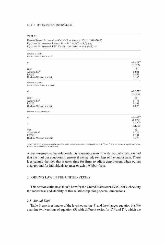
Table 1 reports estimates of the levels equation (3) and the changes equation (4). Weexamine two versions of equation (3) with different series for Ut* and Yt*, which we


TABLE 2

UNITED STATES: ESTIMATES OF OKUN’S LAW (QUARTERLY DATA, 1948Q1–2013Q4)EQUATION ESTIMATED IN LEVELS: Ut − Ut

∗ = β(L)(Yt − Yt∗) + εt

EQUATION ESTIMATED IN FIRST DIFFERENCES: �Ut = α + β(L)�Yt + εt

Equation in levels Equation in differences

Hodrick–Prescott filter λ

1,600 1,600 16,000 16,000

β0 −0.440** −0.251** −0.428** −0.221** −0.288** −0.220**

(0.020) (0.020) (0.023) (0.024) (0.027) (0.018)β1 −0.133** −0.153** −0.140**

(0.026) (0.036) (0.021)β2 −0.122** −0.088* −0.073**

(0.024) (0.035) (0.014)β0+β1+β2 −0.506** −0.462** −0.432**

(0.021) (0.023) (0.035)α 0.239** 0.351**

(0.037) (0.038)Observations 264 262 264 262 263 261Adjusted R2 0.770 0.867 0.786 0.842 0.486 0.647RMSE 0.395 0.299 0.490 0.422 0.285 0.237Durbin–Watson stat. 0.583 0.508 0.377 0.262 1.397 1.396

NOTE: This table reports point estimates and Newey–West standard errors in parentheses. ** and * indicate statistical significance at the 1%and 5% level, respectively.

create by choosing different smoothing parameters in the HP filter. We try smoothingparameters of λ = 100 and λ = 1,000, the most common choices for annual data.

Our three specifications yield similar results. The estimates of the coefficient β arearound –0.4, and the R2s range from 0.72 to 0.80. The levels equation with an HPparameter of λ = 100 yields the best fit by a small margin.

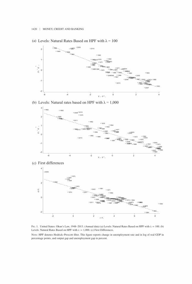
Figure 1 illustrates the fit of Okun’s Law by plotting Ut – Ut* against Yt – Yt*, andthe change in U against the change in Y. We see that our simple versions of the lawexplain most fluctuations in unemployment since 1948.

2.2 Quarterly Data

Table 2 presents estimates of Okun’s Law in levels and changes based on quarterlydata. For the levels specification, we again estimate Ut* and Yt* with the HP filter; wetry smoothing parameters of λ = 1,600 and λ = 16,000, which are common choicesfor quarterly data. We present results with only the current output variable in theequation, and also with two lags included.

For the levels specification with no lags, the estimated Okun coefficients are–0.44 and –0.43, near the estimates with annual data. When lags are included, thecoefficients on the current Yt – Yt* are smaller, and the two lags are significant,implying modest delays in the full adjustment of unemployment to output. The sumsof the coefficients on current and lagged output are –0.51 and –0.46 for the two


(a)

(b)

(c)

FIG. 1. United States: Okun’s Law, 1948–2013. (Annual data) (a) Levels: Natural Rates Based on HPF with λ = 100. (b)Levels: Natural Rates Based on HPF with λ = 1,000. (c) First Differences.

NOTE: HPF denotes Hodrick–Prescott filter. This figure reports change in unemployment rate and in log of real GDP inpercentage points, and output gap and unemployment gap in percent.


0

2

4

6

8

10

12

1950 1960 1970 1980 1990 2000 2010

Actual Fitted

FIG. 2. United States: Actual and Fitted Unemployment Rate, 1948Q2–2013Q4.

NOTE: Figure reports fitted unemployment rate from Okun specification estimated on quarterly data in levels with twolags and natural rates based on Hodrick–Prescott filter with λ = 1,600.

values of λ. When the lags are included, the R2s are as high as 0.87 (for λ = 1,600),a nonnegligible improvement on the R2s with annual data.2

For the changes specification, the quarterly results are slightly less robust. With nolags, the coefficient on the change in output is only –0.29; when lags are included,the sum of coefficients is –0.43, close to the results for the levels specification. TheR2 is on the low side with no lags (0.49), and rises to 0.65 when lags are included.Evidently, in quarterly data, the Okun relationship in changes is somewhat noisierthan the relationship in levels.

We illustrate the fit of our levels specification by calculating fitted values for theunemployment rate. With lags included, these fitted values are

Ut = U ∗t + β0

(Yt − Y ∗

t

) + β1(Yt−1 − Y ∗

t−1

) + β2(Yt−2 − Y ∗

t−2

), (5)

where Ut* and Yt* are long-run levels from the HP filter, and the βs are estimatedcoefficients on the current and lagged output gaps. In this exercise, we use a smoothingparameter of λ = 1,600 in the HP filter. Figure 2 compares the paths over time ofUt and of actual unemployment Ut. We see that unemployment is close to the levelpredicted by Okun’s Law throughout the period since 1948.

2. For the levels specification, we have also estimated a version of Okun’s Law with two lags of thedependent variable, U – U*, as well as current and two lags of Y – Y*. For λ = 1,600, the estimatedcoefficients on the lags of U – U* are 0.95 and −0.26, and the coefficients on current Y – Y* and its lagsare −0.23, 0.06, and 0.01. Using repeated substitution, we can derive a reduced form in which U – U*depends only on Y–Y* and its lags, and the sum of coefficients is −0.49. This equation is qualitativelysimilar to the second column of Table 2, in which the sum of coefficients on Y – Y* and its lags is −0.51.


TABLE 3

OKUN’S LAW AND RECESSIONS

EQUATION ESTIMATED IN LEVELS (1)–(4): Ut − Ut∗ = β(L)(Yt − Yt

∗) + γ (L)Rect + δ(L)(Yt − Yt∗)Rect

+ εt

EQUATION ESTIMATED IN FIRST DIFFERENCES (5)–(8): �Ut = α + β(L)�Yt + γ (L)Rect + δ(L)�Yt Rect + εt

(1) (2) (3) (4) (5) (6) (7) (8)

α 0.351** 0.158** 0.250** 0.122**

(0.038) (0.041) (0.044) (0.040)β0 + β1 + β2 −0.506** −0.488** −0.474** −0.468** −0.432** −0.283** −0.343** −0.248**

(0.021) (0.025) (0.028) (0.028) (0.035) (0.037) (0.038) (0.037)γ 0 + γ 1 + γ 2 0.031 −0.099 0.474** 0.396**

(0.108) (0.108) (0.070) (0.063)δ0 + δ1 + δ2 −0.113* −0.127* −0.432** −0.287**

(0.053) (0.057) (0.114) (0.075)Obs 262 262 262 262 261 261 261 261Adjusted R2 0.867 0.871 0.872 0.874 0.647 0.727 0.689 0.743RMSE 0.299 0.296 0.294 0.292 0.237 0.209 0.223 0.203


2.3 Stability

We have found that simple versions of Okun’s Law, which are linear and fixed overour 66-year sample, yield a good fit to the short-run relationship between output andunemployment. Yet a number of previous studies question the fit of a simple Okun’sLaw. Some, such as Knotek (2007), suggest a nonlinearity: the effect of output onunemployment is larger during recessions than during expansions. Others, such asMeyer and Tasci (2012), suggest that the coefficient in Okun’s Law varies over time.

Here, we examine these ideas. Using quarterly data, we find some evidence ofdeviations from a stable, linear Okun’s Law. However, as shown below, in economicterms, the sizes of these deviations are modest—especially for the levels version ofOkun’s Law. This finding reflects the fact that the simple specifications in Table 2produce R2s as high as 0.87. There is little scope for generalizations of the equationsto improve their fit.

Effects of recessions. We estimate quarterly specifications that allow deviations fromthe usual Okun’s law during NBER recessions. We examine both our levels equation(with λ = 1,600) and our changes equation, and allow recessions to alter Okun’sLaw in two ways. First, we introduce a dummy variable for a quarter that is partof a recession, and two lags of this dummy. These terms allow a fixed effect ofthe recession state on the level or change in unemployment. Second, we includeinteractions between the dummy variable and the output gap or change in output,again with two lags. These terms allow the output coefficient in Okun’s Law to differbetween expansions and recessions.

Table 3 reports the results. For the levels Okun’s law, the estimated effects ofrecessions are modest. The dummy variable and its lags are jointly insignificant,and the interactions between the dummy and output gaps are borderline significant


(t = 2.2). Including these extra terms raises the R2 only from 0.867 to 0.874. Basedon point estimates, the sum of coefficients on the output gap and its lags is −0.47 inexpansions and −0.60 in recessions (−0.60 is the sum of coefficients on the gap plusthe sum of coefficients on the gap–recession interactions).

The equation for unemployment changes suggests larger effects of recessions. Boththe recession dummies and their interactions with output changes are statisticallysignificant, and including those terms raises the R2 from 0.65 to 0.74. These resultsconfirm our earlier finding that the changes version of Okun’s Law is less robust thanthe levels version (see Table 2).

To get a sense of how a recession can shift Okun’s Law, we consider the economyin the first quarter of 2009, the height of the Great Recession. In that quarter, outputgrowth (not annualized) was −1.4%, and its two lags were −2.1% and −0.5%. Therecession dummy and its two lags were all 1. For this observation, the fitted value forthe change in the unemployment rate is 1.0 in our basic changes version of Okun’sLaw, and 1.3 in the version that accounts for recessions. The actual unemploymentchange in 2009Q1 was 1.4.

Time variation in coefficients. For our linear Okun’s Law equations, we test forstability over time, focusing on the sum of coefficients on current output and its twolags. We first test for equality of this sum for the periods 1948–83 and 1984–2014. Wechoose 1984 as a break point because it is the beginning of the “Great Moderation”period in U.S. macroeconomic history. Some researchers suggest that the labor marketchanged during this period; Gali and van Rens (2014), for example, argue thatfrictions in hiring fell, which could increase the responsiveness of employment andunemployment to output fluctuations.

The first part of Table 4 reports results, which are similar for the levels anddifferences versions of Okun’s Law. We find that the sum of output coefficients rosesomewhat in absolute value in our second subsample. For the levels equation, the sumof coefficients is −0.48 before 1984 and −0.61 after; for the changes specification,the corresponding numbers are −0.42 and −0.51. The differences across periods arestatistically significant.

On the other hand, allowing different coefficients for the two periods makes almostno difference for the fit of our equations. Starting from an equation with stablecoefficients, allowing the coefficients to change increases the R2 from 0.87 to 0.88for the levels specification and from 0.65 to 0.66 for the changes specification. Theseresults suggest that an Okun’s Law with constant coefficients is a good approximationto reality.

We also test for the stability of our equations using the Andrews (2003) sup-Waldtest with an unknown break date. Stability is again rejected, with break dates assuggested by the largest Wald statistic of 2003Q4 for the levels equation and 2004Q1for the differences equation. In both cases, the sum of coefficients for the second,shorter subsample is larger in absolute value than the sum for the first subsample. Forthe levels specification, the sum of coefficients is −0.48 before 2003Q4 and −0.78after.


TABLE 4

OKUN’S LAW: ALLOWING FOR A STRUCTURAL BREAK

EQUATION ESTIMATED IN LEVELS: Ut − U ∗t = βt<τ (L)(Yt − Y ∗

t ) + βt≥τ (L)(Yt − Y ∗t ) + εt

EQUATION ESTIMATED IN FIRST DIFFERENCES: �Ut = α + βt<τ (L)�Yt + βt≥τ (L)�Yt + εt

With break With break

Levels Fixed Estimated Changes Fixed Estimatedbaseline τ = 1984Q1 τ = 2003Q4 baseline τ = 1984Q1 τ = 2004Q1

β0 + β1 + β2 −0.506** −0.432**

(0.021) (0.035)t < τ : β0 + β1 + β2 −0.477** −0.476** −0.417** −0.423**

(0.017) (0.016) (0.033) (0.033)t � τ : β0 + β1 + β2 −0.608** −0.778** −0.512 −0.708**

(0.053) (0.029) (0.040) (0.057)F 5.474 84.565 8.861 26.651p 0.020 0.000 0.003 0.000Adjusted R2 0.867 0.876 0.894 0.647 0.658 0.674


Yet, once again, allowing a change in coefficients yields only a modest improve-ment in the fit of Okun’s Law. The R2 rises from 0.87 to 0.89 for the levels equation,and from 0.65 to 0.67 for the differences equation.

We can gain further perspective from Figure 2, which shows the fit of a levelsOkun’s Law with constant coefficients. Starting in the early 2000s, when the Andrewstest identifies a break, we see larger ups and downs in actual unemployment than infitted unemployment. For example, from 2006Q4 to 2009Q4, actual unemploymentrises by 5.5 percentage points (from 4.4% to 9.9%) and the fitted value rises only4.2 points (from 5.0% to 9.2%). This pattern is consistent with a rise in the Okuncoefficients near the end of the sample. However, the deviations between actual andfitted unemployment shown in Figure 2 are modest compared to the fluctuationsin unemployment over time. Again, a stable Okun’s Law appears to be a goodapproximation to reality.3

2.4 Comparison to Okun (1962)

We find that Okun’s 50-year old specification yields a good fit to data from 1948through 2013. Yet our coefficient estimates differ somewhat from those in Okun’soriginal paper. Okun estimated that a 1% increase in output causes the unemploymentrate to fall by about 0.3 percentage points. Inverting this coefficient, he positedthe rule of thumb that a one-point change in unemployment occurs when outputchanges by 3%. Our coefficient estimates, by contrast, are around –0.4 or –0.5. These

3. Some papers (e.g., Meyer and Tasci 2012) argue for instability in Okun’s Law based on rollingregressions. This is an informal test where the amount of estimated instability depends heavily on thewindow width. We prefer the sup-F-test where we can apply the statistical theory developed by Andrews.


TABLE 5

UNITED STATES: REPLICATION AND UPDATE OF OKUN’S (1962) REGRESSION

(QUARTERLY DATA) EQUATION ESTIMATED: �Ut = α + β0�Yt + β1�Yt−1 + β2�Yt−2 + εt

1948Q2–1960Q4 1948Q2–2013Q4

Vintage data Current data

Sample (1) (2) (3) (4)

β0 −0.307** −0.233** −0.288** −0.220**

(0.039) (0.023) (0.027) (0.018)β1 −0.168** −0.140**

(0.030) (0.021)β2 −0.039** −0.073**

(0.019) (0.014)β0+β1+β2 −0.441** −0.432**

(0.044) (0.035)α 0.305** 0.424** 0.239** 0.351**

(0.076) (0.069) (0.037) (0.038)Obs 51 51 263 261Adjusted R2 0.584 0.758 0.486 0.647RMSE 0.382 0.292 0.285 0.237Durbin–Watson stat. 1.625 1.580 1.397 1.396


estimates fit roughly with modern textbooks, which report an inverted coefficientof 2.

Why do our coefficient estimates differ from Okun’s? The natural guess is differ-ences in data—either the sample period or the vintage of the data. But that is not thecase; instead, the differences in results arise from differences in the specification ofOkun’s Law.

This point is easiest to see for the changes version of the law, where the key specifi-cation issue is lag structure. Okun estimates the changes equation, our equation (4), inquarterly data with no lags. Based on data for 1947Q2 through 1960Q4, he reports acoefficient of –0.30. When we estimate the same specification for our longer sample,the coefficient is almost the same: −0.29. For the changes equation, we obtain largercoefficients only if we use annual data or include lags in our quarterly specification(see Tables 1 and 2).

To pin down this issue, Table 5 reports quarterly estimates of the changes equationwith and without lags of output growth. We compare estimates for two periods:our full sample, and 1948Q2–1960Q4, which is our best approximation of Okun’ssample with currently available data. For Okun’s sample, we use 1965Q4 vintagedata for output, which should be close to the data that Okun used.4 With no lags,

4. The 1965Q4 vintage data are the earliest vintage of data for real GNP/GDP availablefrom the Federal Reserve Bank of Philadelphia Real-Time Data Set for Macroeconomists (http://www.philadelphiafed.org/research-and-data/real-time-center/real-time-data/data-files/ROUTPUT/). Theresults are similar if we use the 1948Q2–1960Q4 sample and current (revised) data.

http://www.philadelphiafed.org/research-and-data/real-time-center/real-time-data/data-files/ROUTPUT/

http://www.philadelphiafed.org/research-and-data/real-time-center/real-time-data/data-files/ROUTPUT/


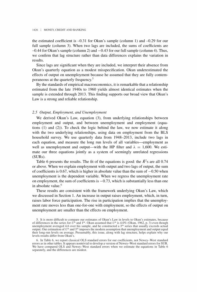
the estimated coefficient is –0.31 for Okun’s sample (column 1) and –0.29 for ourfull sample (column 3). When two lags are included, the sums of coefficients are–0.44 for Okun’s sample (column 2) and −0.43 for our full sample (column 4). Thus,we confirm that lag structure rather than data differences explains the variation inresults.

Since lags are significant when they are included, we interpret their absence fromOkun’s quarterly equation as a modest misspecification. Okun underestimated theeffects of output on unemployment because he assumed that they are fully contem-poraneous at the quarterly frequency.5

By the standards of empirical macroeconomics, it is remarkable that a relationshipestimated from the late 1940s to 1960 yields almost identical estimates when thesample is extended through 2013. This finding supports our broad view that Okun’sLaw is a strong and reliable relationship.

2.5 Output, Employment, and Unemployment

We derived Okun’s Law, equation (3), from underlying relationships betweenemployment and output, and between unemployment and employment (equa-tions (1) and (2)). To check the logic behind the law, we now estimate it alongwith the two underlying relationships, using data on employment from the BLShousehold survey. We use quarterly data from 1948–2013, include two lags ineach equation, and measure the long run levels of all variables—employment aswell as unemployment and output—with the HP filter and λ = 1,600. We esti-mate our three equations jointly as a system of seemingly unrelated regressions(SURs).

Table 6 presents the results. The fit of the equations is good: the R2s are all 0.74or above. When we explain employment with output and two lags of output, the sumof coefficients is 0.67, which is higher in absolute value than the sum of −0.50 whenunemployment is the dependent variable. When we regress the unemployment rateon employment, the sum of coefficients is −0.73, which is substantially less than onein absolute value.6

These results are consistent with the framework underlying Okun’s Law, whichwe discussed in Section 1. An increase in output raises employment, which, in turn,raises labor force participation. The rise in participation implies that the unemploy-ment rate moves less than one-for-one with employment, so the effects of output onunemployment are smaller than the effects on employment.

5. It is more difficult to compare our estimates of Okun’s Law in levels to Okun’s estimates, becauseof differences in the series for U* and Y*. Okun assumed that U* is 4.0% (Okun, 1962, p. 3) even thoughunemployment averaged 4.6 over his sample, and he constructed a Y* series that usually exceeds actualoutput. Our estimation of U* and Y* imposes the modern assumption that unemployment and output equaltheir long-run levels on average. Presumably, this issue, along with lag structure, helps explain why ourlevels results differ from Okun’s.

6. In Table 6, we report classical OLS standard errors for our coefficients, not Newey–West standarderrors as in other tables. It appears nontrivial to develop a version of Newey–West standard errors for SUR.We have compared OLS and Newey–West standard errors when we estimate the equations in Table 6separately, and the differences are modest.


TABLE 6

UNITED STATES: ESTIMATES OF OKUN’S LAW AND UNEMPLOYMENT–EMPLOYMENT RELATION (QUARTERLY DATA,1948Q1–2013Q4)SEEMINGLY UNRELATED REGRESSIONS

Equation in levels

Hodrick–Prescott filter λ = 1,600

Ut −Ut* = β(L)(Yt −Yt

*)+εt Et −Et* = β(L)(Yt −Yt

*)+εt Ut −Ut* = β(L)(Et −Et

*)+εt

β0 −0.240** 0.314** −0.736**

(0.023) (0.035) (0.022)β1 −0.134** 0.181** −0.010

(0.034) (0.051) (0.031)β2 −0.122** 0.176** 0.019

(0.023) (0.035) (0.020)β0+β1+β2 −0.496** 0.670** −0.728**

(0.012) (0.020) (0.013)Obs 262 262 262Adjusted R2 0.869 0.739 0.843Durbin–Watson 0.503 0.503 0.503

NOTE: Table reports point estimates and standard errors in parentheses. ** and * indicate statistical significance at the 1% and 5% level,respectively.

3. JOBLESS RECOVERIES?

Many observers suggest that Okun’s Law has broken down in a particular way:recoveries following recessions have become “jobless,” with weaker employmentgrowth and higher unemployment than Okun’s Law predicts (e.g., Gordon 2010).The recoveries from the last three U.S. recessions—those of 1990–91, 2001, and2008–2009—have all been called jobless. Many economists treat the emergence ofjobless recoveries as a fact to be explained. In 2011, for example, Barcelona’s Centerfor International Economic Research held a conference on “Understanding JoblessRecoveries” that focused on the three U.S. episodes.

We can look for evidence of jobless recoveries in the Figure 2 discussed earlier. Af-ter the 1990 and 2008 recessions, unemployment peaks at higher levels than its fittedvalues according to Okun’s Law. This fact implies some unexplained “joblessness”—but the deviations from Okun’s Law are far too small to suggest a qualitative changein the nature of recoveries. After the 2001 recession, the peak unemployment rate isalmost exactly the same as its fitted value. As we have stressed before, the overallmessage of Figure 2 is that Okun’s Law does not change much over time or phasesof the business cycle.

A potentially important nuance is that economists who discuss jobless recoveries,such as Schreft and Singh (2003) and Gordon (2010), often examine the behaviorof employment rather than the unemployment rate. In principle, a recovery might bejobless in the sense of subnormal employment growth, yet not produce an anomalousrise in the unemployment rate, if labor force participation falls.


Δ

Δ

FIG. 3. United States: Okun’s Law for Employment: Actual and Fitted Values.

NOTE: The label is the first quarter of the recovery.

To investigate this possibility, we examine the behavior of employment duringrecoveries. Specifically, we examine employment growth in the first four quartersafter an NBER trough, the recovery period studied by Schreft and Singh (2003).

In this exercise, we first estimate the normal output–employment relationship inquarterly differences: we regress the change in log employment on the change inlog output and its first two lags. We then compute fitted values of the change in logemployment, average these fitted values over four-quarter periods, and compare theseaverages to actual changes in log employment. Figure 3 shows the results for all four-quarter periods in our sample, and highlights the recoveries following NBER troughs.This figure tells us whether employment growth during recoveries is unusually lowconditional on output growth.7

In Figure 3, the observations marked by black dots are the recovery periods afterthe last three NBER troughs—the allegedly jobless recoveries. In all three episodes,the fitted value of the change in employment is greater than the actual change. Intwo cases, however, the difference is trivial. In the third case—the recovery after theGreat Recession of 2008–09—the difference is somewhat larger, but the observationis hardly an outlier. Overall, the figure shows that employment growth has not beenanomalous in recent recoveries.

If the employment–output relationship has not shifted, then why have observersseen recent recoveries as jobless? Galı, Smets, and Wouters (2012) give the answer:recoveries since 1990 have been weaker than earlier recoveries. We can see thisfact in Figure 3, where gray squares mark the eight recoveries between 1948 and1990. These observations lie above and to the right of the more recent recoveries:actual employment growth is higher and so are fitted values, because of higher outputgrowth. Averaging across the two groups of recoveries, employment growth fell from2.5% before 1990 to −0.1% after 1990, and output growth fell from 7.3% to 2.5%.

7. In the estimated equation for the change in log employment, the constant is −0.46 and the coefficientson the change in log output and its two lags are 0.22, 0.23, and 0.047.


9.5

9.6

9.7

9.8

2007 2009 2011 2013 2015

Real GDP

4

6

8

10

2007 2009 2011 2013 2015

Unemployment rate

11.8

11.9

12

2007 2009 2011 2013 2015

Employment

58

59

60

61

62

63

2007 2009 2011 2013 2015

Employment-to-population ratio

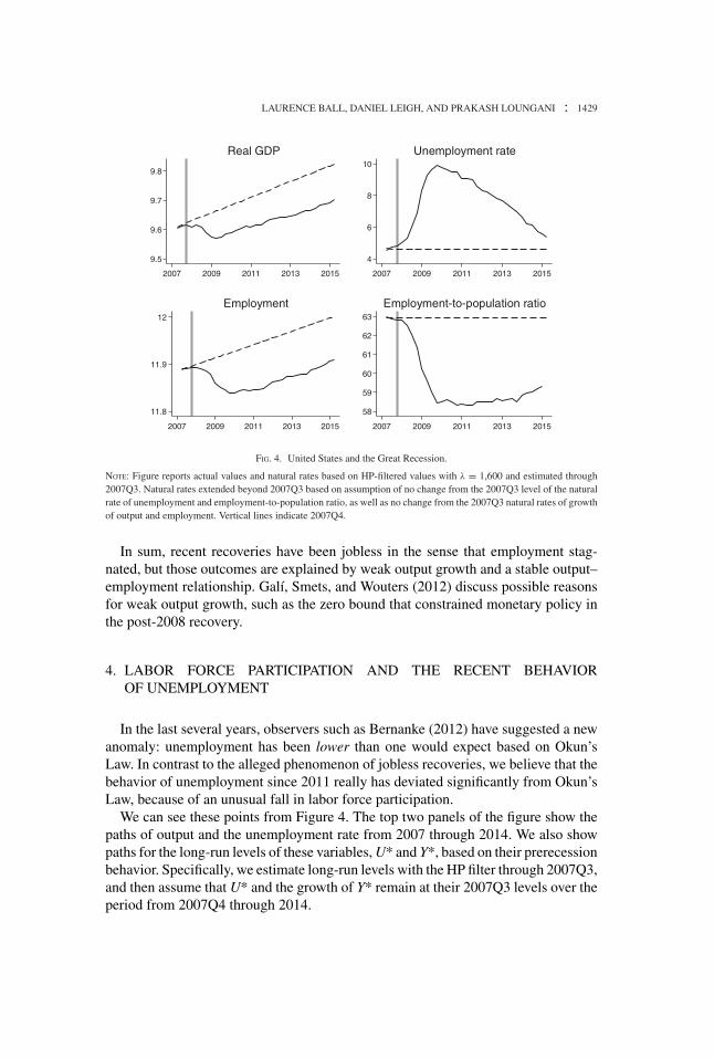
FIG. 4. United States and the Great Recession.

NOTE: Figure reports actual values and natural rates based on HP-filtered values with λ = 1,600 and estimated through2007Q3. Natural rates extended beyond 2007Q3 based on assumption of no change from the 2007Q3 level of the naturalrate of unemployment and employment-to-population ratio, as well as no change from the 2007Q3 natural rates of growthof output and employment. Vertical lines indicate 2007Q4.

In sum, recent recoveries have been jobless in the sense that employment stag-nated, but those outcomes are explained by weak output growth and a stable output–employment relationship. Galı, Smets, and Wouters (2012) discuss possible reasonsfor weak output growth, such as the zero bound that constrained monetary policy inthe post-2008 recovery.

4. LABOR FORCE PARTICIPATION AND THE RECENT BEHAVIOROF UNEMPLOYMENT

In the last several years, observers such as Bernanke (2012) have suggested a newanomaly: unemployment has been lower than one would expect based on Okun’sLaw. In contrast to the alleged phenomenon of jobless recoveries, we believe that thebehavior of unemployment since 2011 really has deviated significantly from Okun’sLaw, because of an unusual fall in labor force participation.

We can see these points from Figure 4. The top two panels of the figure show thepaths of output and the unemployment rate from 2007 through 2014. We also showpaths for the long-run levels of these variables, U* and Y*, based on their prerecessionbehavior. Specifically, we estimate long-run levels with the HP filter through 2007Q3,and then assume that U* and the growth of Y* remain at their 2007Q3 levels over theperiod from 2007Q4 through 2014.


For the first part of the period in Figure 4, from 2007 through 2011, the dataare consistent with Okun’s Law. In 2011Q4, the estimated deviations of outputand unemployment from their long run levels are −10% and 4 percentage points,respectively, suggesting an Okun coefficient of −0.4, close to our estimates for theUnited States since 1948. But after 2011, we see a substantial fall in unemploymentthat is not consistent with Okun’s Law. The output gap widens by about 2 percentagepoints from 2011Q4 to 2014Q4, which should imply a slight rise in unemployment,but the estimated unemployment gap decreases by almost 3 percentage points.

What explains this deviation from Okun’s Law? It was not caused by anomalousbehavior of employment. The bottom two panels of Figure 4 make this point by show-ing the paths of employment and the employment-population ratio (e-pop), along withtheir long run levels (once again estimated through 2007Q3 and then extrapolated).In contrast to the unemployment rate, employment and e-pop do not return towardtheir prerecession paths after 2011. Rather, the gap between employment and its longrun level widens slightly, consistent with the slight increase in the output gap.

Recall that Okun’s Law (equation (3) above) is derived from underlying rela-tionships between employment and output (equation (1)), and between unemploy-ment and employment (equation (2)). Figure 4 suggests that the employment–outputrelationship has not shifted substantially in recent years, but unemployment hasfallen by more than Okun’s Law predicts; in other words, we have seen stability inequation (1) but instability in equation (3). We can reconcile these facts ifequation (2) has shifted—specifically, if the unemployment rate has fallen by morethan we would expect based on employment. That happens if there is an unusualdecrease in labor force participation.

And indeed, there has been a substantial fall in the labor force participation rate,from 66% in 2008Q4 to 63% in 2014Q4. As discussed by Erceg and Levin (2013),this decrease is far greater than expected based on the behavior of output and themodest procyclicality of participation before 2008.

The explanation for the fall in participation is not clear. Some economists citedemographic changes and other trends that began before 2008, such as rising schoolenrollments (e.g., Krueger 2016). Erceg and Levin, by contrast, emphasize the unusualdepth and duration of the Great Recession. In their view, costs of entering andexiting the labor force normally mean that participation does not respond much toemployment fluctuations, but a protracted recession eventually leads workers to exit.

5. OKUN’S LAW IN 20 ADVANCED ECONOMIES

Here, we examine the fit of Okun’s Law in 20 countries: those with populationsabove one million that were members of the OECD in 1985. We use data on outputand unemployment from the OECD.8

8. We present results for OECD data based on national definitions of unemployment. The results aresimilar when we use the OECD’s harmonized unemployment series.


TABLE 7

ADVANCED ECONOMIES: ESTIMATES OF OKUN’S LAW

EQUATION ESTIMATED:QUARTERLY: Ut − Ut

∗ = β0(Yt − Yt∗) + β1(Yt−1 − Yt−1

∗) + β2(Yt−2 − Yt−2∗) + εt

ANNUAL: Ut − Ut∗ = β(Yt − Yt

∗) + εt

Quarterly data (1980Q1–2013Q4) Annual data (1980–2013)

Levels version

β0+β1+β2 Adjusted R2 β Adjusted R2

Australia −0.554** (0.042) 0.748 −0.563** (0.046) 0.785Austria −0.172** (0.029) 0.264 −0.132** (0.035) 0.156Belgium −0.476** (0.056) 0.590 −0.538** (0.097) 0.600Canada −0.524** (0.031) 0.811 −0.443** (0.035) 0.785Denmark −0.434** (0.033) 0.700 −0.434** (0.042) 0.677Finland −0.420** (0.061) 0.694 −0.490** (0.089) 0.749France −0.370** (0.036) 0.672 −0.353** (0.039) 0.665Germany −0.304** (0.055) 0.488 −0.363** (0.091) 0.461Ireland −0.415** (0.043) 0.538 −0.384** (0.049) 0.613Italy −0.217** (0.040) 0.253 −0.295** (0.089) 0.301Japan −0.151** (0.014) 0.643 −0.165** (0.023) 0.705Netherlands −0.451** (0.055) 0.635 −0.520** (0.102) 0.609New Zealand −0.335** (0.059) 0.370 −0.397** (0.058) 0.659Norway −0.261** (0.031) 0.497 −0.272** (0.036) 0.609Portugal −0.310** (0.029) 0.471 −0.308** (0.038) 0.718Spain −0.939** (0.067) 0.742 −0.824** (0.059) 0.866Sweden −0.434** (0.071) 0.638 −0.538** (0.111) 0.607Switzerland −0.256** (0.028) 0.575 −0.222** (0.031) 0.425United Kingdom −0.360** (0.048) 0.665 −0.357** (0.070) 0.559United States −0.563** (0.039) 0.846 −0.476** (0.047) 0.779


5.1 Basic Results

We examine the period from 1980 to 2013. We start our samples in 1980 because,in a number of countries, unemployment was very low in earlier periods. An extremeexample is New Zealand, where unemployment rates between 1960 and 1975 rangedfrom 0.04% to 0.66%. Evidently, some countries’ economic regimes in the 1960s and1970s differed from those of more recent decades, or unemployment was measureddifferently.

For each country in our sample, Table 7 reports estimates of Okun’s Law in levels.We report a version with annual data, with Ut* and Yt* measured with an HP parameterof λ = 100, and a version with quarterly data, with an HP parameter of 1,600 andtwo lags of the output gap in the equation.

The fit is good for most countries, though usually not as close as for theUnited States. The R2 exceeds 0.4 in all countries but Austria and Italy for an-nual data, and for all but Austria, Italy, and New Zealand for quarterly data. The


average R2 for the 20 countries is 0.62 for annual data and 0.59 for quarterlydata.9

The estimated coefficients on the output gap vary considerably across countries.For annual data, most coefficients are spread between –0.27 and –0.55, but three arelower in absolute value (Austria, Japan, and Switzerland), and Spain is an outlier with–0.82. The average coefficient is −0.40. The results for quarterly data are similar:the average of the sum of coefficients is −0.40, and the correlation across countriesbetween this sum and the annual coefficient is 0.94. Spain is even more of an outlierin quarterly data, with a sum of coefficients of −0.94.

Countries with higher R2’s generally have higher coefficients. Japan, however, isan exception: it has fairly high R2s (0.71 in annual data) but low coefficients (–0.17in annual data). Japan’s unemployment movements are small and are well explainedby its output movements and a low coefficient in Okun’s Law.

As a robustness check, Table 8 reports estimates of the differences version ofOkun’s Law, both annual and quarterly. Averaging across countries, the Okun coeffi-cients are somewhat smaller than those in the levels equation: the average coefficientfalls from −0.40 to −0.32 for annual data, and for quarterly data, the sum of coeffi-cients falls from −0.40 to −0.31. Yet, the variation in coefficients across countries isquite similar for levels and differences. For annual data, the cross-country correlationof the level and difference coefficients is 0.92, and for quarterly data, the correlationof the sums of coefficients is 0.94.

5.2 Stability over Time

We now ask whether the Okun’s Law coefficient is stable over time in a givencountry. Previous studies have suggested that it is not stable: Cazes, Verick, andAl-Hussami (2011) find that the coefficient varies erratically in many countries, andIMF (2010) finds that it has generally risen over time. The IMF study’s explanationis that legal reforms have reduced the costs of firing workers.

We have examined the stability of our annual and quarterly specifications of Okun’sLaw in levels (Table 7). An online Appendix presents detailed results. Following ourapproach with U.S. data, we first do simple stability tests with a fixed break date.We break the sample in half, estimating separate coefficients for 1980–96 and 1997–2013.

We find some evidence of instability. With annual data, we reject stability of theOkun coefficient at the 5% level for 7 of the 20 countries. However, in five of theseseven cases, the coefficient is lower in absolute value in the second half of the sample.The average coefficient for the 20 countries is –0.44 in the first half of the sample and–0.34 in the second. The quarterly results are not very different: there is a significantchange in the sum of output coefficients in nine countries, and five of these changesare decreases in absolute value. Our data generally do not support the view that theOkun coefficient has risen over time.

9. We estimate the Okun coefficient for each country with OLS. The results are similar if we estimatethe coefficients jointly in a panel framework with SURs.


TABLE 8

ADVANCED ECONOMIES: ESTIMATES OF OKUN’S LAW

EQUATION ESTIMATED:QUARTERLY: � Ut = α + β0�Yt + β1�Yt−1 + β2�Yt−2 + εt

ANNUAL: � Ut = α + β�Yt + εt

Quarterly data (1980Q1–2013Q4) Annual data (1980–2013)

Changes version

β0+β1+β2 Adjusted R2 β Adjusted R2

Australia −0.410** (0.061) 0.455 −0.461** (0.064) 0.628Austria −0.204** (0.034) 0.108 −0.135** (0.032) 0.168Belgium −0.317** (0.087) 0.177 −0.315** (0.072) 0.357Canada −0.433** (0.070) 0.500 −0.433** (0.049) 0.766Denmark −0.326** (0.034) 0.414 −0.346** (0.043) 0.557Finland −0.354** (0.076) 0.398 −0.347** (0.105) 0.521France −0.331** (0.035) 0.389 −0.274** (0.039) 0.409Germany −0.229** (0.053) 0.290 −0.223* (0.082) 0.245Ireland −0.327** (0.067) 0.376 −0.348** (0.065) 0.528Italy −0.187** (0.056) 0.123 −0.170* (0.073) 0.179Japan −0.075** (0.026) 0.193 −0.079** (0.020) 0.306Netherlands −0.315** (0.054) 0.423 −0.363** (0.094) 0.459New Zealand −0.165** (0.041) 0.109 −0.310** (0.062) 0.408Norway −0.120** (0.038) 0.063 −0.171** (0.040) 0.274Portugal −0.312** (0.043) 0.149 −0.304** (0.040) 0.659Spain −0.744** (0.094) 0.578 −0.802** (0.090) 0.786Sweden −0.423** (0.083) 0.507 −0.388** (0.124) 0.486Switzerland −0.205** (0.034) 0.293 −0.188** (0.045) 0.377United Kingdom −0.322** (0.051) 0.505 −0.326** (0.059) 0.562United States −0.443** (0.049) 0.625 −0.430** (0.047) 0.731


The differences in coefficients across countries are similar in the two time periods.For example, the annual coefficient for Spain is the highest in both periods, and thosefor Austria, Switzerland, and Japan are among the lowest. Overall, the correlation ofannual coefficients across the two periods is 0.42.

For our quarterly specification, we have also performed the Andrews test for a breakat an unknown date. With that test, stability of the sum of coefficients is rejected at the5% level for 13 of the 20 countries. Once again, the number of significant decreasesin coefficients exceeds the significant increases, 8 to 5. The break dates, as identifiedby the largest Wald statistic, vary widely across countries: from 1985 in Canada and1988 in Switzerland to 2008 in Germany and France. This heterogeneity in resultssuggests that there was no international change in Okun’s Law during any particulartime period.10

10. For an alternative perspective, see Daly et al (2014), who argue that Okun’s Law coefficientschanged around 2008 in many countries.


6. OKUN’S LAW IN THE GREAT RECESSION

Skepticism about Okun’s Law has grown in the wake of the Great Recession of2008–09. One reason, emphasized by IMF (2010), Bakker and Zeng (2014), andMcKinsey Global Institute (2011), is that there is little correlation across countriesbetween decreases in output and increases in unemployment during the countries’recessions. Once again, we believe that claims of a breakdown in Okun’s Law areexaggerated.

6.1 Output and Unemployment from Peak to Trough

We can see why a quick look at the data might suggest a breakdown of Okun’s Law.Nineteen of the countries in our sample (all but Australia) experienced a recessionthat began in either late-2007 or 2008, according to Harding and Pagan’s (2002)definitions of peaks and troughs in output. For these countries, Figure 5(a) plots thechange in output from peak to trough against the change in unemployment over thesame period. This figure is similar to one in IMF (2010).

The figure shows that changes in output and unemployment are uncorrelated acrosscountries. When the change in U is regressed on a constant and the change in Y, theR2 is –0.002. Commentators have used subsets of the observations in Figure 5(a) asan evidence against Okun’s Law. McKinsey, for example, points out that Germanyand the United Kingdom had larger output falls than the United States and Spain,yet unemployment increased by less in the UK and fell in Germany. Bakker andZeng (2014) cite Ireland and Spain as countries where unemployment rose more thanOkun’s Law predicts.

Such evidence has led researchers to propose novel factors to explain unemploy-ment changes. IMF (2010) suggests that financial crises and house price busts raiseunemployment for a given level of output. McKinsey suggests that output growthmay fail to decrease unemployment because workers lack the skills for availablejobs.

6.2 Correcting for the Length of Recessions

It is misleading to compare output and unemployment changes during differentcountries’ recessions, because recessions last for varying lengths of time. For theset of recessions in Figure 5(a), the period from peak to trough ranges from twoquarters in Portugal to seven quarters in Denmark. Okun’s Law implies a relation-ship between the changes in unemployment and output only if we control for thisfactor.

To see this point in a simple way, suppose that the changes version of Okun’s Lawholds exactly in quarterly data:

�Ut = α + β�Yt , α > 0, β < 0, (6)


ΣΔ

Σ Δ

ΣΔ

α β Σ Δ

ΣΔ

α β Σ Δ

(a)

(b)

(c)

FIG. 5. The Great Recession: Peak-to-Trough Output and Unemployment Changes. (a) Simple Scatter Plot. (b) Adjustmentfor T. (c) Adjustment for T and Country-Specific Okun Coefficients.

NOTE: � �U and � �Y denote the cumulative peak-to-trough change in the unemployment rate and in the log of realGDP, respectively. T denotes the duration of the recession (peak to trough in quarters). αi and β i denote country-specificOkun coefficients.


where for the moment, we assume that the parameters α and β are the same for allcountries. Let T be the number of quarters in a recession. Cumulating equation (6)over T quarters gives

� �U = α T + β� �Y, (7)

where � indicates the cumulative change over a recession.Recall that α > 0 because potential output grows over time. Thus, holding con-

stant the change in output, a longer recession implies a larger rise in unemployment.With potential output on an upward path, a given absolute fall in output trans-lates into a larger output gap and higher unemployment if it occurs over a longerperiod.

We examine the fit of equation (7) across countries by regressing the cumu-lative change in U during a country’s recession on the cumulative change in Yand the recession length T (without a constant term). This regression yields esti-mates of α = 0.63 (standard error = 0.30) and β = –0.08 (standard error = 0.22).Figure 5(b) plots the cumulative change in U against the fitted values from this regres-sion. We see that the version of Okun’s Law in equation (7) explains a substantial partof the cross-country variation in � �U: the R2 is 0.53. Notice that Spain is less ofan outlier than it was in Figure 5(a). The large increase in Spanish unemployment ispartly explained by the length of Spain’s recession—six quarters, the second longestin the sample.

6.3 Adjusting for Country-Specific Coefficients

We saw in Section 5 that the coefficient in Okun’s Law varies substantially acrosscountries. We now ask whether changes in unemployment during the Great Recessionfit the law, given the usual coefficient for each country. That is, we examine thefit of

� �U = αi T + βi� �Y, (8)

where αi and β i are the parameters of Okun’s Law for country i.We compute the fitted values of � �U implied by equation (8). For αi and

β i, we use estimates of Okun’s Law in changes for annual data over 1980–2013(with αi divided by four to fit the current exercise with quarterly data). The αisaverage 0.84 across countries (0.21 once we divide by four). The β is are given inTable 8.

Figure 5(c) compares the actual and fitted values of � �U. We see that equation (8)fits well: the R2 is 0.77. Again, Spain is a good example. Its large rise in unemploymentis explained almost entirely by the fact that its Okun coefficient β i is unusually large,along with the length of its recession. In other words, Spain did experience a largerrise in unemployment than other countries, but that is what we should expect basedon its historical Okun’s Law.


6.4 A German Miracle?

When economists discuss deviations from Okun’s Law, many stress the recentexperience of Germany. As Figure 5 shows, Germany is the one country whereunemployment fell during its recession, an outcome that is often called a “miracle”(e.g., Burda and Hunt 2011). Many economists explain this experience with work-sharing—decreases in hours per worker—encouraged by government subsidies toemployers who retained workers.

Figure 5(c) confirms that Germany deviated from Okun’s Law during its recession.Its predicted change in unemployment was 2 percentage points, and its actual changewas –0.3 percentage points. This episode reminds us that Okun’s Law does notexplain 100% of unemployment behavior. Yet “miracle” may be an exaggeration ofGermany’s experience. The residual in Germany’s Okun’s Law is modest comparedto cross-country differences in unemployment changes.

7. EXPLAINING CROSS-COUNTRY VARIATION IN OKUN’S LAW

We have seen that Okun’s Law fits the data in most countries, but that the Okuncoefficient differs across countries. What explains these differences? In addressingthis question, we focus on the levels version of Okun’s Law estimated with annualdata.

7.1 Looking for Explanatory Variables

We can gain some insight about the Okun coefficient from Figure 6, which plotsthe estimated annual coefficients for our 20 countries against the average levelof unemployment over 1980–2013 (left panel). We see an inverse relationship: incountries where unemployment is higher on average, it also fluctuates more in re-sponse to output movements. This result is driven primarily by a cluster of coun-tries with low unemployment and low coefficients—Switzerland, Japan, Austria, andNorway—and by Spain, which has very high unemployment and a very high coeffi-cient. It appears likely that the underlying factors that determine the Okun coefficientalso influence average unemployment.

We have looked for the underlying determinants of the Okun coefficient, but ourresults are largely negative. A notable failure is the OECD’s well-known index ofemployment protection legislation (EPL). In theory, greater employment protectionshould dampen the effects of output movements on employment and therefore reducethe Okun coefficient. In Figure 6 (right panel), we test this idea by plotting thecoefficient against the OECD’s overall EPL index (averaged over 1985–2008, theperiod for which it is available). The relationship has the wrong sign, and it isstatistically insignificant.11

11. For New Zealand, the EPL index is available over 1990–2008. We also find no relationship betweenthe Okun coefficient and the various components of the EPL index.


FIG. 6. Explaining Cross-Country Variation in Okun Coefficients (Okun Coefficient versus Candidate Variables).

NOTE: Average unemployment rate denotes 1980–2013 mean. OECD overall employment protection index denotes1985–2008 mean based on available data.

7.2 Individual Countries

We can also learn about the Okun coefficient by examining individual countries.It appears that the labor markets of many countries have idiosyncratic features thatinfluence the coefficient. These features—not one or two variables that we can mea-sure for all countries—probably account for most of the variation in the coefficient.To support this idea, we examine the country with the highest estimated coefficient,Spain, and the three countries with the lowest coefficients (focusing again on thelevels equation with annual data).

Spain. This country’s Okun coefficient, –0.82, is substantially higher in absolutevalue than any other country’s. The natural explanation is the unusually high incidenceof temporary employment contracts. Labor market reforms in the 1980s made iteasier for Spanish employers to hire workers on fixed-term contracts, without theemployment protection guaranteed to permanent workers. Over the 1990s and 2000s,such contracts have accounted for around a third of Spanish employment. Temporarycontracts make it easier for firms to adjust employment when output changes, raisingthe Okun coefficient.

Notice that the OECD’s EPL index assigns a fairly high number to Spain, suggest-ing that it is not easy for Spanish employers to adjust employment. However, closeobservers of Spain argue that the OECD index is not a good measure of flexibility in


this case. One reason is that the OECD does not account for the nonenforcement ofde jure restrictions on fixed-term contracts (Bentolila et al. 2010).

Japan. This country’s Okun coefficient, –0.17, is the second smallest in absolutevalue. The likely explanation is Japan’s tradition of “lifetime employment,” whichmakes firms reluctant to lay off workers. This feature of the labor market is achoice of employers, not a legal mandate, and therefore is not captured by the EPLindex.

Ono (2010) reports that the lifetime employment tradition has weakened somewhatover time. This suggests that Japan’s Okun coefficient may have risen—and indeed,Japan is one of the two countries with a statistically significant increase in thecoefficient from the first half of our sample period to the second (see online Appendix).However, the coefficient is low compared to other countries in both parts of the sample(−0.12 in the first and −0.22 in the second).

Switzerland. This country’s coefficient, –0.22, is the third smallest. A likely expla-nation is the large use of foreign workers in Switzerland. When employment rises orfalls, migrant workers move in and out of the country. Changes in employment areaccommodated by changes in the labor force, and unemployment is stable.

Recall that Okun’s Law is derived from an employment–output relationship, equa-tion (1), and an unemployment–employment relationship, equation (2). We estimatethese two equations for our 20 countries and examine where Switzerland lies in theranges of coefficients. Switzerland’s coefficient in the E-Y equation, 0.49, is nearthe middle of the range for the 20 countries. Switzerland’s coefficient in the U-Eequation is the second smallest, and it is statistically insignificant. These results con-firm that Switzerland’s unusual feature is the nonresponsiveness of unemployment toemployment.

Austria. Austria’s data are puzzling. Its Okun coefficient, –0.13, is the smallest for our20 countries, and we have not found an explanation for this result. When we estimatethe E-Y and U-E relationships, the coefficients are 0.16 and −0.04, respectively. Bothcoefficients are the lowest (in absolute value) for our set of 20 countries and the latterestimate is implausibly small. We leave further investigation of Austria for futureresearch.

8. CONCLUSION

It is rare to call a macroeconomic relationship a “law.” Yet we believe that Okun’sLaw has earned its name. It is not as universal as the law of gravity (which has the sameparameters in all advanced economies), but it is strong and stable by the standards ofmacroeconomics. Reports of deviations from the Law are often exaggerated. Okun’sLaw is certainly more reliable than a typical macrorelationship like the Phillips curve,which is constantly under repair as new anomalies arise in the data.


The evidence in this paper is consistent with traditional macromodels in whichshifts in aggregate demand cause short-run fluctuations in unemployment. At thispoint, we do not claim that the evidence is not consistent with other theories of un-employment, such as those based on sectoral shocks or extensions of unemploymentbenefits. The usefulness of Okun’s Law in testing macrotheories is a topic for futureresearch.

A possible starting point is the fact that the Okun coefficient is far smaller than onewould expect from an inverted production function (even when we put employmentrather than unemployment on the left side of the law). Traditional macro explains thisfact with costs of adjusting employment to aggregate demand shifts. It is not clearwhether a small Okun’s coefficient arises naturally in other models of unemployment.

LITERATURE CITED

Andrews, Donald W. K. (2003) “Tests for Parameter Instability and Structural Change withUnknown Change Point: A Corrigendum.” Econometrica, 71, 395–7.

Bakker, Bas, and Li Zeng. (2014) “Reducing the Employment Impact of Corporate BalanceSheet Repair.” In Jobs and Growth: supporting the European Recovery 2014, edited bySpilimbergo Antonio, Berger Helge, Bas Bakker, and Schindler Martin, pp. 39–66. Wash-ington, DC: International Monetary Fund.

Bentolila, Samuel, Pierre Cahuc, Juan Dolado, and Thomas Le Barbanchon. (2010) “Two-TierLabor Markets in the Great Recession: France vs. Spain.” IZA DP No. 5340.

Bernanke, Ben. (2012) “Recent Developments in the Labor Market.” Speech at theNational Association for Business Economics Annual Conference, Arlington, TX.https://www.federalreserve.gov/newsevents/speech/bernanke20120326a.htm

Blanchard, Olivier. (2011) Macroeconomics, 5th ed. Upper Saddle River, NJ: Prentice Hall.

Burda, Michael C., and Jennifer Hunt. (2011) “What Explains the German Labor MarketMiracle in the Great Recession?” NBER Working Paper No. 17187.

Cazes, Sandrine, Sher Verick, and Fares Al-Hussami. (2011) “Diverging Trends in Unemploy-ment in the United States and Europe: Evidence from Okun’s Law and the Global FinancialCrisis.” Employment Working Papers, ILO.

Daly, Mary C., John G. Fernald, Oscar Jorda, and Fernanda Nechio. (2012) “Okun’s Macro-scope: Output and Employment after the Great Recession.” Manuscript, Federal ReserveBank of San Francisco.

Erceg, Christopher J., and Andrew T. Levin. (2013) “Labor Force Participation and MonetaryPolicy in the Wake of the Great Recession.” IMF Working Paper 13/245.

Galı, Jordi, Frank Smets, and Rafael Wouters. (2012) “Slow Recoveries: A Structural Inter-pretation.” NBER Working Paper No. 18085.

Gali, Jordi, and Thijs van Rens. (2014) “The Vanishing Procyclicality of Labor Productivity.”Warwick Economic Research Papers No. 1062.

Gordon, Robert J. (2010) “Okun’s Law and Productivity Innovations.” American EconomicReview, 100, 11–5.

Harding, Don, and Adrian Pagan. (2002) “Dissecting the Cycle: A Methodological Investiga-tion.” Journal of Monetary Economics, 49, 365–81.

https://www.federalreserve.gov/newsevents/speech/bernanke20120326a.htm


International Monetary Fund (IMF). (2010) “Unemployment Dynamics during Recessions andRecoveries: Okun’s Law and Beyond.” In World Economic Outlook, April 2010: RebalancingGrowth, pp. 69–107. Washington, DC: International Monetary Fund.

Knotek, Edward S. (2007) “How Useful Is Okun’s Law?” Economic Review, 4, 73–103.

Krueger, Alan. (2016) “Where Have All the Workers Gone?” Presented at Federal ReserveBank of Boston 60th Annual Economic Conference. Princeton University & NBER.

Mankiw, N. Gregory. (2012) Principles of Macroeconomics, 6th ed. New York, NY: ThomsonNelson.

McKinsey Global Institute. (2011) “An Economy That Works: Job Creation and America’sFuture.” June 2011 Report.

Meyer, Brent, and Murat Tasci. (2012) “An Unstable Okun’s Law, Not the Best Rule ofThumb.” Economic Commentary, Federal Reserve of Cleveland.

Newey, Whitney K., and Kenneth D. West. (1987) “A Simple, Positive Semi-Definite, Het-eroskedasticity and Autocorrelation Consistent Covariance Matrix.” Econometrica, 55, 703–8.

Oi, Walter Y. (1962) “Labor as a Quasi-Fixed Factor.” Journal of Political Economy, 70,538–55.

Okun, Arthur M. (1962) “Potential GNP: Its Measurement and Significance.” Reprinted asCowles Foundation Paper 190.

Ono, Hiroshi. (2010). “Lifetime Employment in Japan: Concepts and Measurements.” Journalof the Japanese and International Economies, 24, 1–27.

Phillips, Peter C. B., and Sainan Jin. (2015). “Business Cycles, Trend Elimination, and the HPFilter.” Cowles Foundation Discussion Paper No. 2005.

Prachowny, Martin F. J. (1993) “Okun’s Law: Theoretical Foundations and Revised Estimates.”Review of Economics and Statistics, 75, 331–6.

Schreft, Stacey L., and Aarti Singh. (2003) “A Closer Look at Jobless Recoveries.” FederalReserve Bank of Kansas City Economic Review, 88, 45–73.

okun's law: fit at 50? - johns hopkins university

Documents