oligopolistic capacity expansion with subse- quent market
TRANSCRIPT

Final Report 7.12.2017
Oligopolistic capacity expansion with subse-quent market-bidding under transmission constraints (OCESM)

Oligopolistic capacity expansion with subsequent market-bidding under transmission constraints (OCESM)
2/91
Datum: 7. December 2017
Ort: Villigen PSI
Auftraggeberin:
Bundesamt für Energie BFE
Forschungsprogramm EWG
CH-3003 Bern
www.bfe.admin.ch
Auftragnehmer/in:
Energy Economics Group
Paul Scherrer Institut (PSI)
5232 Villigen PSI
www.psi.ch/eem
Chair of Quantitative Business Administration
University of Zurich
Moussonstrasse 15, 8044 Zürich
http://www.business.uzh.ch/de/professorships/qba/
Autor/in:
Evangelos Panos, Paul Scherrer Institute
Martin Densing (PI), Paul Scherrer Institute, [email protected]
Karl Schmedders (PI), University of Zurich
BFE-Bereichsleitung: Matthias Gysler, [email protected]
BFE-Programmleitung: Florian Kämpfer, [email protected]
BFE-Vertragsnummer: SI/501119-01
The authors only are responsible for the content and the conclusions of this report. The views
expressed in this paper do not necessarily represent those of the SFOE.
Bundesamt für Energie BFE
Mühlestrasse 4, CH-3063 Ittigen; Postadresse: CH-3003 Bern
Tel. +41 58 462 56 11 · Fax +41 58 463 25 00 · [email protected] · www.bfe.admin.ch

3/91
Abstract
We investigate the investment and market behaviour of power producers on European electricity mar-
kets. The key driver of investment and production in a liberalised environment is the market price (with
the exception of investments in new renewables, which are also policy driven). Market players usually
do not cooperate to maximise social welfare, such that the assumption of purely production cost re-
lated decisions of a central planner may not be correct. Hence, the main goal is to model prices under
different policy scenarios.
The employed numerical model is a game-theoretic electricity market model for Switzerland and its
surrounding countries. The players are aggregated on country level for this first phase of model devel-
opment that was initiated by this BFE-EWG project. The model is technology detailed having different
power-supply options including also thermal production constraints as well as hydropower energy stor-
age. We analyse different scenarios at the target year 2035, where nuclear power is assumed to be
phased out in Germany and Switzerland, under different assumptions of fossil fuel and CO2 prices, of
availability of lignite power in Germany, and different price-demand elasticities than today.
The main conclusions include that changes in the supply mix in Switzerland (hydro availability, deploy-
ment of new renewables etc.) have minor influence on Swiss wholesale electricity prices; the trade
with the surrounding countries determine the price for Switzerland, which is a price-taker. The gas
price will determine strongly the wholesale price in Switzerland, even when Switzerland is not in-
stalling gas plants in our profit-driven market modelling; new renewables are installed exogenously
driven by the policy per scenario. Nevertheless, under low gas (and CO2) prices, Swiss electricity
price levels and price volatility can stay approximately as of today, even under the expected capacity
changes in Switzerland and surrounding countries.
Zusammenfassung
Untersucht wird das Investitions- und Marktverhalten von Stromerzeugern im Europäischen Marktum-
feld. Der wesentliche Faktor für Investitionen und Stromerzeugung in einem liberalisierten Marktumfeld
ist der Marktpreis (mit Ausnahme der Investitionen in neue Erneuerbare, die auch politikgesteuert sein
können). Marktteilnehmer kooperieren gewöhnlich nicht zur Maximierung eines Gesamtnutzens, so
dass die Annahme einer Entscheidungsfindung eines zentralen Planers aufgrund nur der Produktions-
kosten nicht korrekt ist. Darum ist das Hauptziel die Modellierung von Strompreisen unter verschiede-
nen Politik-Szenarien.
Das verwendete numerische Modell ist ein spieltheoretisches Strommarkt-Modell für die Schweiz und
die umliegenden Länder. Für die erste Modellierungsphase, die durch dieses BFE-EWG Projekt initi-
iert wurde, sind die Marktteilnehmer auf Länderebene aggregiert. Das Model ist technologisch detail-
liert mit verschieden Stromerzeugungs-Optionen, die auch thermische Erzeugungsrestriktionen und
die Energiespeicherung der Wasserkraft beinhalten. Wir analysieren verschiedene Szenarien für das
Jahr 2035 (in dem Kernkraft in Deutschland und der Schweiz nicht mehr existieren) unter verschiede-
nen Annahmen fossiler Brennstoff- und CO2-Preise, der Verfügbarkeit von Braunkohle in Deutsch-
land, und von Preis-Nachfrage Elastizitäten.
Die Schlussfolgerungen beinhalten dass Änderungen im Erzeugungsmix der Schweiz (Verfügbarkeit
von Wasserkraft, Installation neuer Erneuerbarer etc.) einen geringen Einfluss auf die Schweizer

Oligopolistic capacity expansion with subsequent market-bidding under transmission constraints (OCESM)
4/91
Grosshandelspreise haben; der Handel mit den umliegenden Ländern bestimmt den Preis des Preis-
nehmers Schweiz. Der Gaspreis wird den Grosshandelspreis der Schweiz massgeblich bestimmen,
auch wenn die Schweiz keine eigenen Gaskraftwerke baut gemäss unserer profit-orientierten Markt-
modellierung; der Zubau neuer Erneuerbarer ist exogen bestimmt gemäss Szenario-Annahme. Nichts-
destotrotz könnte das Schweizer Preisniveau und die Preis-Volatilität in Szenarien tiefer Gas- und
CO2-Preise ungefähr auf heutigem Niveau bleiben, auch unter Berücksichtigung der erwarteten Kapa-
zitätsverschiebungen in der Schweiz und umliegender Ländern.
Résumé
Nous étudions le comportement sur le marché et en matière d’investissements de producteurs d’élec-
tricité dans le contexte du marché européen. Le facteur clé des investissements et de la production
d’électricité dans un environnement de marché libéralisé est le prix du marché (à l’exception des in-
vestissements dans les nouvelles énergies renouvelables qui peuvent aussi être soutenues par les
pouvoirs publics). Les acteurs du marché ne coopèrent en général pas pour maximiser un bénéfice
global. L’hypothèse selon laquelle les décisions d’un planificateur central ne seraient prises qu’en
fonction des coûts de production n’est donc pas correcte. C’est pourquoi l’objectif principal est de mo-
déliser les prix de l’électricité selon différents scénarios politiques.
Le modèle numérique utilisé est un modèle du marché de l’électricité fondé sur la théorie des jeux et
valable pour la Suisse et les pays environnants. Pour la première phase de modélisation initiée par ce
projet OFEN-EES, les acteurs du marché sont agrégés au niveau national. Le modèle est technologi-
quement détaillé et comporte diverses options de production d’électricité incluant les contraintes liées
à la production thermique ainsi que le stockage de l’énergie hydraulique. Nous analysons différents
scénarios pour l’année 2035 (date à laquelle l’énergie nucléaire devrait être bannie en Allemagne et
en Suisse) en fonction de diverses hypothèses sur les prix du carburant fossile et du carbone, la dis-
ponibilité du lignite en Allemagne et l’élasticité de la demande par rapport aux prix.
Les conclusions montrent que des changements dans le mix de production de la Suisse (disponibilité
de l’énergie hydraulique, introduction de nouvelles énergies renouvelables, etc.) ont une faible in-
fluence sur les prix de gros de l’électricité en Suisse; les échanges avec les pays voisins déterminent
le prix pour la Suisse qui est un preneur de prix. Le prix du gaz déterminera fortement le prix de gros
en Suisse, même si la Suisse ne construit pas de centrales au gaz selon notre modélisation du mar-
ché orientée sur le profit; le développement de nouvelles énergies renouvelables est défini de façon
exogène en fonction de l’hypothèse du scénario. Dans des scénarios de prix bas du gaz et du car-
bone, le niveau et la volatilité des prix en Suisse pourraient néanmoins être à peu près les mêmes
qu’aujourd’hui, même en tenant compte des changement de capacité attendus en Suisse et dans les
pays environnants.

5/91
Contents
Abbreviations / Conventions ................................................................................................................ 7
1. Key Messages ............................................................................................................................. 8
1.1. Project Highlights .......................................................................................................................... 8
1.2. Key Messages ............................................................................................................................... 8
2. Introduction ............................................................................................................................... 10
2.1. Project goals ............................................................................................................................... 10
2.2. Market modelling ......................................................................................................................... 10
2.3. Load periods within the target year ............................................................................................. 14
2.4. Profit optimization problem of each player .................................................................................. 14
2.4.1. TSO’s distribution problem ..................................................................................................... 17
2.5. Technical constraints on thermal generation ............................................................................... 19
2.6. Storage ........................................................................................................................................ 22
2.7. Constraints on production (hourly, daily, seasonally) .................................................................. 24
2.8. Modelling of hydropower storage ................................................................................................ 26
2.9. Numerical model solving ............................................................................................................. 28
2.9.1. Open-Loop: PATH solver ....................................................................................................... 28
2.9.2. Closed-Loop: Diagonalization ................................................................................................ 29
3. Data Input ................................................................................................................................... 30
4. Calibration (Scenario “today”) ................................................................................................ 33
5. Scenarios ................................................................................................................................... 43
5.1. Scenario Definition ...................................................................................................................... 43
5.1.1. Base 2035 Scenario („Base“)................................................................................................. 44
5.1.2. No Lignite Production Scenario (“noLignite”) ......................................................................... 47
5.1.3. Low Gas Price Scenario (“lowGas”) ...................................................................................... 47
5.1.4. Today’s Cost Scenario (“todayCost”) ..................................................................................... 47
5.1.5. High CO2 Price Scenario (“CO2”) ........................................................................................... 48
5.1.6. High Price-Demand Elasticity Scenario (“CO2 + Elast”) ........................................................ 48
5.2. Scenario Results ......................................................................................................................... 49
5.2.1. Future electricity prices .......................................................................................................... 49
5.2.2. Endogenous Production and Investment ............................................................................... 60
5.2.3. Cross-border electricity flows ................................................................................................. 66
5.2.4. Profit of power production ...................................................................................................... 69
6. Auxiliary Results ....................................................................................................................... 73
6.1. Marginal (high-cost) technology .................................................................................................. 73
6.2. Closed Loop results .................................................................................................................... 79
7. Auxiliary Analyses .................................................................................................................... 81

Oligopolistic capacity expansion with subsequent market-bidding under transmission constraints (OCESM)
6/91
7.1. Empirical analysis of supply, price, and demand ........................................................................ 81
7.1.1. Price, Market volume, Demand.............................................................................................. 81
7.1.2. Elasticities of demand-bids at EPEX ..................................................................................... 82
7.1.3. Empirical analysis of merit order curve of Germany .............................................................. 83
7.2. Statistical decomposition of wind and solar availability .............................................................. 85
8. Auxiliary Project Information ................................................................................................... 88
8.1. Dissemination .............................................................................................................................. 88
8.2. Personnel / Acknowledgment ...................................................................................................... 88
9. References ................................................................................................................................. 89

7/91
Abbreviations / Conventions
AT Austria
BEM model Bi-level electricity market model
CAPEX Capital expenditure
CH Switzerland
DE Germany
DE+AT Coupled market area of Germany and Austria
EPEC Equilibrium problem with equilibrium constraints
EPEX European power exchange
FIXOM Fixed Operating & Maintenance costs
FR France
Gas-CC Gas-fuelled combined-cycle plants
GME Italian power market (Gestore Mercati Energetici)
IT Italy
MCP Mixed Complementarity Program
MPEC Mathematical program with equilibrium constraints
NTC Net transfer capacity (between market areas)
OCESM Oligopolistic capacity expansion with sub-sequent market-bidding under trans-
mission constraints
OTC Over-the-counter marketing (not EPEX/GME)
RoR Run-of-River hydropower
TSO Transmission system operator
VAROM Variable Operating & Maintenance costs
Conventions:
Winter Dec + Jan + Feb
Spring Mar + Apr + May
Summer Jun + Jul + Aug
Fall Sep + Oct + Nov
Biomass Biomass + Waste

Oligopolistic capacity expansion with subsequent market-bidding under transmission constraints (OCESM)
8/91
1. Key Messages
1.1. Project Highlights
The project, which was partially financed by the SFOE, helped to better establish Nash-Cournot
market modelling in Switzerland. During the project, a numerical wholesale market model was
developed. The market model is envisaged to be able to capture wholesale (day-ahead) market
price trends under a variety of policy scenarios, which is not possible with purely econometric
or central-planner optimisation models.
Capturing future market prices is challenging because prices are determined by the interplay
between supply- and demand-offers in specific market time slots, leading occasionally to price
peaks (scarcity effects) which cannot be explained only by merit-order cost curves. Assuming
that such scarcity effects as of today will prevail, we investigate how investments in new renew-
ables and how exogenously given fossil fuel prices influence electricity market prices.
With the developed market model, which is still experimental, we can investigate profit-driven
investment decisions in conventional technologies under the assumption that such investments
are entirely driven by market forces (superseding the central planner perspective of power pro-
duction).
1.2. Key Messages
Market prices cannot be sufficiently explained by perfect-competition energy optimisation mod-
els (social welfare maximisation, central planner perspective). Comparison of our market model
in normal and in social welfare (fall-back) mode shows that the social welfare solution underes-
timates prices. Hence, a (numerical) market model that takes into account deviations from mar-
ginal costs is needed for an attempt to forecast future price ranges under different policy options
and to evaluate possible ranges of profit for utilities and consumers.
Electricity market prices in Switzerland are highly determined by the supply mix of the surround-
ing countries. During all numerical experiments, changes in the supply mix in Switzerland (hydro
availability etc.) had minor influences on Swiss electricity prices; the complex interactions with
the surrounding countries determine the price for Switzerland, which is a small player.
Large new gas power plants do not emerge in the domestic Swiss electricity production mix in
all scenarios in the market model. Nevertheless, future gas prices will determine strongly the
electricity price in Switzerland, even Switzerland is not installing gas plants in our profit-driven
market modelling. Moreover, also in the surrounding countries, the gas price becomes a more
determining factor for prices until the chosen time horizon 2035 because the overcapacity in
Germany and France of other conventional capacity and the nuclear power is expected to be
reduced. Under low gas (and CO2) prices, Swiss electricity price levels and price volatility can
stay approximately at today’s level even under the foreseen capacity changes in Switzerland
and in surrounding countries. Because gas-fuelled plants are likely to have a stronger role as
price-setters on the wholesale markets, raising gas and CO2 prices are directly reflected in rais-
ing wholesale prices in all scenarios in most of the load periods. Hence, it seems—at least for
Switzerland—that the fossil fuel (and CO2) prices will be the major price driver and not the
change in supply mixes. That the capacity mix is not the major driver for Swiss prices holds not
true for all surrounding countries. For example, in France, market prices in the future are ex-
pected to drop because of increased domestic wind generation (Section 5.2.1).

9/91
Germany and Switzerland become net importers of electricity because their domestic capacity
is reduced; in the market model, Switzerland is not expanding its capacity apart from more new
renewables (which is modelled as an exogenous, policy-driven deployment). This impacts for
example the Italian market, because France (which will provide exports to Switzerland and Ger-
many in more load periods) and Switzerland cannot export to Italy as frequently as they do today
to (partially) lower Italian prices during high demand periods. Thus, Italian market prices are
expected to stay relatively high (Section 5.2.1).
Oligopolistic capacity expansion with subsequent market-bidding under transmission constraints (OCESM)
10/91
2. Introduction
2.1. Project goals
The goal of the project is to investigate the investment and market behaviour of power producers on
European electricity markets. The major influence factor of the market on investment and production
decisions in a liberalised market environment is the market price (with the exception of investments in
new renewables, which are also driven by policy actions). Moreover, market players do not cooperate
to maximise social welfare. As a result, purely production cost related decisions of a social planner may
no longer be correct. Hence, the main goal of the project is to capture future prices under different policy
scenarios.
The employed numerical model is an electricity market model for Switzerland and its surrounding coun-
tries; the full project name is OCESM (oligopolistic capacity expansion with subsequent market-bidding
under transmission constraints). The game-theoretic model can analyse scarcity price effects, which
can be caused—among others—by imperfect competition (market power). The players are aggregated
on country levels for the first phase of model development that was initiated by this BFE-EWG project
that is now reported. In the BFE-EWG project, we apply for the majority of the results not the full math-
ematical bi-level setting of the market model, which implies a nested game, but retain the investment
and production decision-making in a single game for various reasons (see below).
The analysis with the model attempts to help regulators to identify influencing key factors of future
wholesale electricity price levels (which impacts also electricity prices of final consumers). Small market
areas (e.g. Switzerland) are strongly influenced by other market areas; for example, the analysis indi-
cates that (non-Swiss based) gas-fuelled plants and the corresponding gas fuel prices are an increas-
ingly important factor. Nevertheless, the analysis may provide decision support to stipulate domestic
(EU market compatible) policy measures that may alleviate the adverse side of external factors. The
scientific aim of the project is to build an electricity market model that resembles closely to the real-world
decision-making process as of today and potentially in the future. In a final, stochastic version of the
model, risk-averse decision making of the players is envisaged to be analysed in the year 2018.
2.2. Market modelling
The model structure, which was implemented as a numerical model is as follows. In the first stage of
the market model, players, which are the power producers, invest in capacity expansion, and in a second
stage, the players produce electricity with newly built (and with partially prevailing old stock of) capacity
(Figure 1). The players of power production are aggregated on a country level, and the buyers of
electricity (wholesale consumers) are represented by an elastic price-demand relationship.
The aggregation of the players on country level has two main reasons. The first reason is that the
production portfolio of the large utilities inside a country are in many cases more similar than between
countries, such that the bidding behaviour of the utilities on the market may also be similar; if there exists
approximately only a single large player (company EdF, France), then the aggregation is obviously
reasonable per se. The second reason is that a split of the production capacity of a country into utilities
is difficult to achieve from the viewpoint of available data, and such a split may change over time; for
example, a plant can belong to several utilities (tough the dispatch is usually governed by a singled-out
utility), or fossil generation of a utility may be outsourced (see the recent case of the split of the company
E.ON in Germany).

11/91
The transmission constraints are modelled with aggregated lines taking into account the physical flows
between the countries and with today’s aggregated line constraints based on the net transfer capacities
(in principle, line constraints can be modelled endogenously, but we keep them as of today in this project
because the production capacities are already changing across the scenarios).
Within the model setup, we can investigate optimal decisions under different exogenous factors, for
example, the influence of future energy policy regulations. In the most general numerical setting, the
model is formulated as an EPEC (equilibrium problem with equilibrium constraints). Hence, the market
model implementation in this full setup is as a bi-level market equilibrium model of Nash-Cournot type,
also called closed-loop model formulation.
Figure 1: Structure of the general market model. Two-stage decision model; 1st stage: investment decision; 2nd
stage: selling of production on the hourly (day-ahead) market. Transmission constraints are evaluated with nodal
pricing schemes. In the stochastic setup, players optimise their expected profit over different scenarios.
A Nash equilibrium is defined as: Given the decision of other players fixed, each player cannot improve
its own decision. See also the very simple game of two players in Figure 2.
Figure 2: Simple non-cooperative game. A pair (x, y) denotes reward x of player 1 and
reward y of player 2 under a certain decision of the players. The decision leading to (3, 3)
is a Nash-equilibrium: Under the assumption that the decisions of all other players are fixed,
any change of a player’s decision leads to a worse result for that player.
In the numerical setup that is applied for most of the analyses for this BFE-EWG project, the model is
used in a more straightforward setup, where the investment and the production decisions are on the
same step. This means that the investment and production decision are decided at once together in a
joint equilibrium between the players (open-loop, MCP formulation), whereas in the closed-loop

Oligopolistic capacity expansion with subsequent market-bidding under transmission constraints (OCESM)
12/91
formulation, there are two separate equilibria: First in time, there will be an equilibrium between the
investors to decide on the investments, then another market equilibrium between the producers of
electricity (closed-loop, EPEC formulation). In this closed-loop formulation, the investors’ equilibrium
decisions anticipate that during production there will also be a second equilibrium, the electricity market
equilibrium. If only one load period is considered, the open-loop formulation has the same solution as
the closed-loop formulation, whereas solutions for models with several load periods may differ only
slightly (Wogrin, 2013). In fact, if there is a single load period, then production is proportional to installed
capacity, such that deciding on production also decides on the required investment for such production
to take place (and vice versa). The reasons why the open-loop formulation is preferred over closed-loop
are as follows.
In Section 6.2, we discuss numerical results in the full bi-level setting (closed-loop); in our
numerical experiments, the differences between the closed-loop model (investment and
production decided in strict sequence) and open-loop model (incremental investment decisions
and corresponding production decision; see also next point) were minor such that we cannot
exclude that the differences are attributable merely to numerical inaccuracies. The cause for the
small differences is that investments are minor, because Central Western Europe has currently
too much capacity in relation to current load levels, and approximately at least 75% of that
capacity is expected to be still present in the scenario’s target year of 2035, such that significant
investments that are not policy (exogenously) driven are absent and only the subsequent
production game is important.
The current market and power supply structure in Central Western Europe makes it unlikely that
several power generation companies play together a long-term (20+ years), one-shot
investment game. It is more likely that (as of today) rather smaller, incremental investment
decisions will be made based on short- and medium-term market outlooks, which are then
exploited by corresponding incremental decision-making. In other words, investments and pro-
duction changes are small and incremental to play save. Because the Nash-equilibrium is
usually interpreted as the limit of an iterative game of players’ unilateral decisions which even-
tually converge to an equilibrium, we consider a joint equilibrium of investment and production
decisions (i.e. the open-loop formulation) to be more realistic.
Apart from the game-theoretic market setting, the model has also a fall-back mode of social welfare
maximisation to compare with conventional electricity optimisation models that have a central planner
perspective. The market model is implemented in the software GAMS and is available to the SFOE on
request. We intend to make the model code open source. The major data sets are described in detail in
the following chapters. Here, we merely give an overview of the different classes of input data:
Supply cost curves by plant type and by country; investment costs per technology
Capacities, potentials, and availabilities (load factors) of the plant types
Loads for each country; elasticity of day-ahead market
Transmission capacity between the countries (nodes)
Estimated market parameter (denoted by θ) to explain the difference between the modelled
supply cost curve and observed prices (caused by scarcity effects)
Many of the data are grouped by the 4*24 = 96 load periods of the model, which represent a typical
day in each of the four seasons of the year. The major output of the model is:
Optimal capacity expansion for each player

13/91
Electricity prices
Electricity flows between players
Optimal production per technology.
The main feature of the market model is the output of wholesale (day-ahead) electricity prices instead
of marginal costs; the marginal cost is the variable production cost of the technology that has highest
variable costs of all technologies selected to produce by the hourly market clearing. Secondary outputs
are the production per technology in the countries (nodes) to satisfy the load; such production mixes are
also a usual output of social welfare maximisation models.
As said, the main purpose of the market model is capturing prices on the day-ahead market. Though, a
large part of the load is satisfied by other forms of contracting, which includes bilateral forward contract-
ing, bilateral short-term contracting, futures, and other derivative contracts with physical delivery.
Moreover, some producers have also their own end-consumer base. It can be assumed that if the num-
ber of market participants increases and becomes very large, the trade on a standardized exchange
platform becomes more relevant than bilaterally negotiated contracting. On the other hand, the hedging
strategies and forecasts of the utilities are expected to become more sophisticated, such that forward
and future contracting may become more important than day-ahead in the future. These two develop-
ments may partially net each other. Moreover, any calibration of the market model is only possible to
today’s prices by capturing the scarcity effects (peak prices) of today’s day-ahead market (because the
day-ahead market of the future is not known; if the day-ahead market regime changes completely, then
the impact on scarcity effects in future market regimes is unknown). Based on this reasoning, we as-
sume the following.
In the model, the day-ahead market share of total power load (in each geographical region)
stays approximately the same as of today. For example, as of today (2015/2016), the volume
of the day-ahead market is approximately 45% of the load in the DE+AT region, 38% in CH,
22% in FR, and 39% in IT (the share of IT is based on proxy data).
To match the load levels of each country, the model calculates the production amount that is not
traded on the day-ahead market, too. As discussed above, this part of the load is currently sat-
isfied by a diverse mix of forward and short-term contracting, over-the-counter agreements and
direct marketing to end-users, and the future share of such contracting may grow or shrink. We
do not attempt a detailed modelling of this heterogeneous part of the load; we just ensure that
the (short-term price-elastic) volume of the day-ahead market plus the non-day-ahead-market
share match together the load that is given exogenously by the different scenarios. This is
achieved through iterative model runs, where the linear demand-price curve is shifted such that
the load is approximately matched.
In summary, several players, which are chosen for this project to represent the aggregated production
portfolios of whole countries, compete for the electricity supply in Switzerland and its neighbouring coun-
tries on the electricity day-ahead market. In fact, implemented (but not used) is the feature that each
player can have her portfolio of power plants to be located at different grid nodes, which in turn do not
have to be in the same country (in the data input in this project: nodes = countries). The base version of
the model is non-stochastic with an average seasonal availability of wind and solar power generation
(in this project), but the stochasticity is fully implemented and will be numerically tested next year.
Oligopolistic capacity expansion with subsequent market-bidding under transmission constraints (OCESM)
14/91
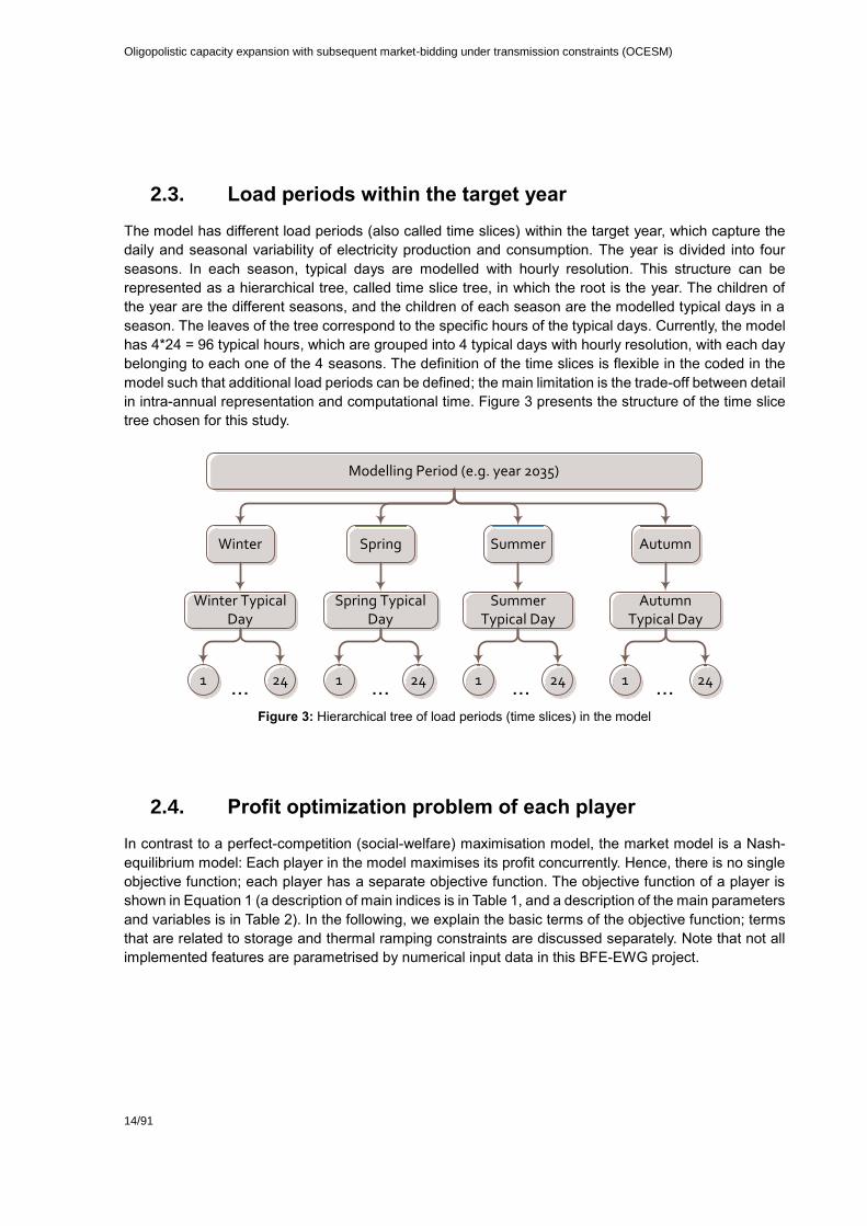
2.3. Load periods within the target year
The model has different load periods (also called time slices) within the target year, which capture the
daily and seasonal variability of electricity production and consumption. The year is divided into four
seasons. In each season, typical days are modelled with hourly resolution. This structure can be
represented as a hierarchical tree, called time slice tree, in which the root is the year. The children of
the year are the different seasons, and the children of each season are the modelled typical days in a
season. The leaves of the tree correspond to the specific hours of the typical days. Currently, the model
has 4*24 = 96 typical hours, which are grouped into 4 typical days with hourly resolution, with each day
belonging to each one of the 4 seasons. The definition of the time slices is flexible in the coded in the
model such that additional load periods can be defined; the main limitation is the trade-off between detail
in intra-annual representation and computational time. Figure 3 presents the structure of the time slice
tree chosen for this study.
Figure 3: Hierarchical tree of load periods (time slices) in the model
2.4. Profit optimization problem of each player
In contrast to a perfect-competition (social-welfare) maximisation model, the market model is a Nash-
equilibrium model: Each player in the model maximises its profit concurrently. Hence, there is no single
objective function; each player has a separate objective function. The objective function of a player is
shown in Equation 1 (a description of main indices is in Table 1, and a description of the main parameters
and variables is in Table 2). In the following, we explain the basic terms of the objective function; terms
that are related to storage and thermal ramping constraints are discussed separately. Note that not all
implemented features are parametrised by numerical input data in this BFE-EWG project.
Modelling Period (e.g. year 2035)
Winter Spring Summer Autumn
Winter Typical Day
Spring Typical Day
Summer Typical Day
Autumn Typical Day
1 24 1 24 1 24 1 24... ... ... ...

15/91
Table 1: Selected indices of the model
In-dex
Description
𝒏 Grid node, 𝒏 = 𝟏, 𝟐, … , 𝑵, where the numbers correspond to counties: AT, DE, FR, IT, CH
𝒊 Player, 𝒊 = 𝟏, 𝟐, … , 𝑰. Currently, in the numerical parametrisation of the market model, play-ers equal countries
𝒋 Power plant type, 𝒋 = 𝟏, 𝟐, … , 𝑱.
𝒌 Transmission line between nodes, 𝒌 = 𝟏, 𝟐, … , 𝑲
𝒔 Probabilistic scenario in the stochastic version of the model, 𝒔 = 𝟏, 𝟐, … , 𝑺
𝒍 Load period, 𝒍 = 𝟏, 𝟐, … , 𝑳
𝑪(𝒕𝒔) Set of load periods which are below 𝒕𝒔 in the tree of time slices (i.e. the load periods that
belong to time slice 𝒕𝒔)
Table 2: Selected parameters of the model (see below for special parameters for storage, ramping, and flow con-
straints)
Parameter Unit Description
�̃�𝑖 - Risk-free return available for player 𝑖. This parameter is not used in this
project. It is meant as a risk-free investment alternative for a player (in-
stead of investing in power supply capacity)
𝛿𝑠 - Weight of probabilistic scenario 𝑠 (stochastic version of the model; not
used for this project)
𝑡𝑙 hours Duration of load period 𝑙
�̃�𝑛𝑖𝑗 EUR/MWh Investment + fixed O&M cost for newly built technology 𝑗 in node 𝑛 for
player 𝑖. The EUR amount is proportional to the number of modelled load
periods per year. The assumed discount rate is 5%.
𝑝𝑛𝑙𝑠0 EUR The intercept of (linear) inverse demand-bid function. Used for elastic
day-ahead market
�̃�𝑛𝑖𝑗 EUR/MWh The slope of (linear) inverse demand-bid function. Used for elastic day-
ahead market
Table 3: Selected variables of the model (see below for individual variables for storage, ramping, and flow con-
straints)
Sym-bol
Unit Description
pnls EUR/MWh Electricity price in node 𝑛, load period 𝑙, and probabilistic scenario 𝑠
anls MWh Export/import in node 𝑛, load period 𝑙, and probabilistic scenario 𝑠
dnls MWh Load in node 𝑛, load period 𝑙, and probabilistic scenario 𝑠
qnijls MWh Quantity of power produced in node 𝑛, by player 𝑖, by technology 𝑗, load pe-
riod 𝑙, and probabilistic scenario 𝑠. This quantity is divided into a production
for the day-ahead market and a remaining part to satisfy the total load.

Oligopolistic capacity expansion with subsequent market-bidding under transmission constraints (OCESM)
16/91
𝑞𝑛𝑖𝑗𝑙𝑠𝑖 MWh Quantity of power stored in node 𝑛, by player 𝑖, by technology 𝑗, load period
𝑙, and probabilistic scenario 𝑠
𝑥𝑛𝑖𝑗 MW investment in technology 𝑗 in node 𝑛, and of player 𝑖
𝑏𝑖 MW Capital invested in risk-free asset (instead of investment in power supply;
not used in this project)
Each player optimises her net profit (Equation 1). The net profit consists of the operating profit, profit &
loss from the wear-down of equipment, and fixed O&M and capital costs from investments; in fact, fixed
costs for existing investments are just an add-on term and can be neglected for the equilibrium solution.
The operational part of the profit is a sum of the profit over each grid node and each technology in a
load period (in the stochastic version of the model, there is an additional sum over the probabilistic
scenarios such that the expected profit is maximised for each player). The operating profit in a load
period, in each grid node, and for each technology is the profit of selling power (i.e. price × quantity)
minus the total of variable costs, which consists of variable O&M costs and of fuel costs.
Equation 1: Objective function of the market model
max𝑥,𝑞,𝑎
�̃�𝑖 𝑏𝑖 + ∑ ∑ (∑ 𝛿𝑠 ∑ 𝑡𝑙(𝑝𝑛𝑙𝑠(𝑞𝑛𝑖𝑗𝑙𝑠 − 𝑞𝑛𝑖𝑗𝑙𝑠i ) − 𝑐𝑛𝑖𝑗𝑠(𝑞𝑛𝑖𝑗𝑙𝑠 + 𝑢𝑗
los𝑞𝑛𝑖𝑗𝑙𝑠l ) − 𝑢𝑗
sucost𝑤𝑛𝑖𝑗𝑙𝑠u
𝐿
𝑙=1
𝑆
𝑠=1
𝐽
𝑗=1
𝑁
𝑛=1
− 𝑢𝑗rucost𝑞𝑛𝑖𝑗𝑙𝑠
u − 𝑢𝑗ruicost𝑞𝑛𝑖𝑗𝑙𝑠
rui − 𝑢𝑗rdcost𝑞𝑛𝑖𝑗𝑙𝑠
d − 𝑢𝑗rdicost𝑞𝑛𝑖𝑗𝑙𝑠
rdi ) − �̃�𝑛𝑖𝑗𝑥𝑛𝑖𝑗 − 𝑐�̅�𝑖𝑗)
Equation 2 lists some of the basic constraints of the market model which are as follows.
Equation 2: Basic constraints of the market model. The variables in parentheses to the right are the shadow
price (dual variable) of the corresponding equation
𝑥𝑛𝑖𝑗0 + 𝑥𝑛𝑖𝑗 ≤ 𝑥𝑛𝑖𝑗
max ∀𝑛, 𝑖, 𝑗 (𝜈𝑛𝑖𝑗 ≥ 0)
𝑞𝑛𝑖𝑗𝑙𝑠 ≤ 𝑓𝑛𝑖𝑗𝑙𝑠max(𝑥𝑛𝑖𝑗
0 + 𝑥𝑛𝑖𝑗 − 𝑤𝑛𝑖𝑗𝑙𝑠o ) ∀𝑛, 𝑖, 𝑗, 𝑙, 𝑠 (𝜇𝑛𝑖𝑗𝑙𝑠 ≥ 0)
𝑓𝑛𝑖𝑗𝑙𝑠min (𝑥𝑛𝑖𝑗
0 + 𝑥𝑛𝑖𝑗 − 𝑤𝑛𝑖𝑗𝑙𝑠o ) ≤ 𝑞𝑛𝑖𝑗𝑙𝑠 ∀𝑛, 𝑖, 𝑗, 𝑙, 𝑠 (𝜉𝑛𝑖𝑗𝑙𝑠
(18)≥ 0)
𝑝𝑛𝑙𝑠 = 𝑝𝑛𝑙𝑠0 + �̃�𝑛𝑖𝑙𝑠(∑ (𝑞𝑛𝑖𝑗𝑙𝑠 − 𝑞𝑛𝑖𝑗𝑙𝑠
𝑖 ) + 𝑎𝑛𝑙𝑠𝐼,𝐽𝑖,𝑗=1 ) ∀𝑛, 𝑙, 𝑠
∑ �̃�𝑛𝑖𝑗𝑥𝑛𝑖𝑗 + 𝑏𝑖 ≤ 𝐾𝑖max𝑁,𝐽
𝑛,𝑗=1 ∀𝑖 (𝜅𝑖 ≥ 0)
(i) The feasible potential of total capacity limits the allowed additional investment in a technology.
This constraint is applied to renewables that have limited potential, and to conventional technol-
ogies that are limited by policy constraints.
(ii) The quantity produced in a load period per technology cannot exceed the available capacity,
which can be time-varying; for example, the available capacity of solar power changes each
hour. The available capacity in a load period is the part of installed capacity that can be started-
up in load period (so-called online capacity). In the opposite direction, there is also a minimal
running constraint based on a minimal availability factor if applicable
17/91
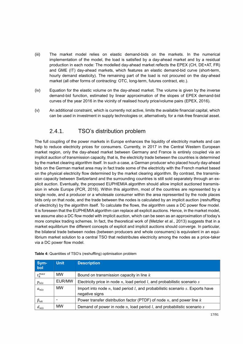
(iii) The market model relies on elastic demand-bids on the markets. In the numerical
implementation of the model, the load is satisfied by a day-ahead market and by a residual
production in each node: The modelled day-ahead market reflects the EPEX (CH, DE+AT, FR)
and GME (IT) day-ahead markets, which features an elastic demand-bid curve (short-term,
hourly demand elasticity). The remaining part of the load is not procured on the day-ahead
market (all other forms of contracting: OTC, long-term, futures contract, etc.).
(iv) Equation for the elastic volume on the day-ahead market. The volume is given by the inverse
demand-bid function, estimated by linear approximation of the slopes of EPEX demand-bid
curves of the year 2016 in the vicinity of realised hourly price/volume pairs (EPEX, 2016).
(v) An additional constraint, which is currently not active, limits the available financial capital, which
can be used in investment in supply technologies or, alternatively, for a risk-free financial asset.
2.4.1. TSO’s distribution problem
The full coupling of the power markets in Europe enhances the liquidity of electricity markets and can
help to reduce electricity prices for consumers. Currently, in 2017 in the Central Western European
market region, only the day-ahead market between Germany and France is entirely coupled via an
implicit auction of transmission capacity, that is, the electricity trade between the countries is determined
by the market clearing algorithm itself. In such a case, a German producer who placed hourly day-ahead
bids on the German market area may in fact trade some of the electricity with the French market based
on the physical electricity flow determined by the market clearing algorithm. By contrast, the transmis-
sion capacity between Switzerland and the surrounding countries is still sold separately through an ex-
plicit auction. Eventually, the proposed EUPHEMIA algorithm should allow implicit auctioned transmis-
sion in whole Europe (PCR, 2016). Within this algorithm, most of the countries are represented by a
single node, and a producer or a wholesale consumer within the area represented by the node places
bids only on that node, and the trade between the nodes is calculated by an implicit auction (reshuffling
of electricity) by the algorithm itself. To calculate the flows, the algorithm uses a DC power flow model.
It is foreseen that the EUPHEMIA algorithm can replace all explicit auctions. Hence, in the market model,
we assume also a DC flow model with implicit auction, which can be seen as an approximation of today’s
more complex trading schemes. In fact, the theoretical work of (Metzler et al., 2013) suggests that in a
market equilibrium the different concepts of explicit and implicit auctions should converge. In particular,
the bilateral trade between nodes (between producers and whole consumers) is equivalent in an equi-
librium market solution to a central TSO that redistributes electricity among the nodes as a price-taker
via a DC power flow model.
Table 4: Quantities of TSO’s (reshuffling) optimisation problem
Sym-bol
Unit Description
𝑡𝑘𝑚𝑎𝑥 MW Bound on transmission capacity in line 𝑘
𝑝𝑛𝑙𝑠 EUR/MW Electricity price in node 𝑛, load period 𝑙, and probabilistic scenario 𝑠
𝑎𝑛𝑙𝑠 MW Import into node 𝑛, load period 𝑙, and probabilistic scenario 𝑠. Exports have
negative signs
𝑝𝑛𝑘 - Power transfer distribution factor (PTDF) of node 𝑛, and power line 𝑘
𝑑𝑛𝑙𝑠 MW Demand of power in node 𝑛, load period 𝑙, and probabilistic scenario 𝑠

Oligopolistic capacity expansion with subsequent market-bidding under transmission constraints (OCESM)
18/91
𝑞𝑛𝑖𝑗𝑙𝑠 MW Quantity of power produced in node 𝑛, by player 𝑖, by technology 𝑗, load pe-
riod 𝑙, and probabilistic scenario 𝑠
𝑞𝑛𝑖𝑗𝑙𝑠𝑖 MW Quantity of power stored in node 𝑛, by player 𝑖, by technology 𝑗, load period
𝑖, and probabilistic scenario 𝑠
Equation 3: TSO’s optimisation problem of social welfare maximisation by reshuffling the electricity between
the nodes. In parentheses: The corresponding shadow price (dual variable) of the constraint
max𝑎
∑ 𝑝𝑛𝑙𝑠𝑎𝑛𝑙𝑠
𝑁,𝐿,𝑆
𝑛,𝑙,𝑠=1
∑ 𝑎𝑛𝑙𝑠 = 0 (𝛾𝑙𝑠)𝑁
𝑛=1
∑ 𝑝𝑛𝑘𝑎𝑛𝑙𝑠 ≤ 𝑡𝑘max
𝑁
𝑛=1 ∀𝑘, 𝑙, 𝑠 (𝜆𝑘𝑙𝑠
+ ≥ 0)
∑ 𝑝𝑛𝑘𝑎𝑛𝑙𝑠 ≥ −𝑡𝑘min
𝑁
𝑛=1 ∀𝑘, 𝑙, 𝑠 (𝜆𝑘𝑙𝑠
− ≥ 0)
𝑑𝑛𝑙𝑠 = ∑ (𝑞𝑛𝑖𝑗𝑙𝑠 − 𝑞𝑛𝑖𝑗𝑙𝑠i ) + 𝑎𝑛𝑙𝑠
𝐼,𝐽
𝑖,𝑗=1
∀𝑛, 𝑙, 𝑠 (𝑝𝑛𝑙𝑠)
The equations of the DC power flow between the grid nodes in the market model are shown in Equation
3. For the required model formulation as a game-theoretic market model with implicit auctioning, the
power flows must also be associated with a player, even such a player cannot actively influence prices
nor produce or consume. We call the problem the TSO’s optimization problem; in fact, the market clear-
ing algorithm determines the flows automatically by matching demand and supply bids; hence, no active
decision is involved. In Equation 3, the objective function is a sum of price × (traded quantity) over all
nodes. The constraints of the problem are as follows.
(i) The balance constraint says that the sum of all export (–anls) and imports (anls) over all nodes
in every load period l (and every probabilistic scenario s; not parametrized in this project)
must be netted to zero.
(ii) The next two sets of constraints are the upper and lower bounds on the transmission ca-
pacity on each line between nodes. The power flow between nodes is induced by the im-
port/export in each node. The so-called power transfer distribution factor (PTDF, denoted
here by 𝑝) determines how much an import/export amount (anls) induces a power flow in a
specific line. In the market model, we assume that each line between nodes has the same
reactance and impedance, because we do not model individual power lines. In fact, this
simplification is correct for trading purposes, because trading decisions are based on ag-
gregated net transfer capacity estimates between the market nodes (NTC).
(iii) The final set of constraints determines how the demand (load) for electricity in a node is
composed as a sum of production in a node, of negative consumption by storage processes
in a node, and of import/export.

19/91
Table 5: Transmission capacity and power transfer distribution factors (PTDFs) in the market model
Capacity Power transfer distribution factors
Nodes / Unit MW DE AT IT FR
DE to AT 2100 0.27 -0.27 -0.07 0.07
DE to CH 2300 0.47 0.20 0.13 0.20
AT to IT 250 0.07 0.27 -0.27 -0.07
AT to CH 800 0.20 0.47 0.20 0.13
IT to FR 1600 -0.07 0.07 0.27 -0.27
IT to CH 1700 0.13 0.20 0.47 0.20
FR to DE 2300 -0.27 -0.07 0.07 0.27
FR to CH 3000 0.20 0.13 0.20 0.47
The assumed transmission capacities are in Table 5. The transmission capacities are based on historical
estimates (2015–2016) of net transfer capacities (NTC). Note that NTCs are the determining limit for
commercial trade. In fact, we have empirically found that the physical power flows are almost always
within the bounds of the NTCs, such that NTCs are a good proxy for real transmission capacity. Note
that the PTDF for Switzerland is not listed in Table 5 because Switzerland is chosen as the so-called
hub node, that is, the associated PTDF is zero, and the flows to and from Switzerland are implied by
those of all other nodes.
2.5. Technical constraints on thermal generation
To reduce problem size and facilitate manageable computation times, a continuous relaxation of the unit
commitment problem, instead of a mixed-integer plant-level formulation, is coupled to the investment
problem. The relaxation is based on a technology-clustered formulation that combines identical or similar
units into clusters. It assumes copper plate and identical techno-economic characteristics of units within
a cluster. The clustering approach reduces the size of the problem since the large set of binary variables
representing the commitment decision of individual units is replaced by linear commitment variables.
The coupling of a linearised formulation of the short-term unit commitment problem with the long-term
investment problem has already been successfully used in (Panos and Lehtila, 2016; van Stiphout et
al., 2016; Palmintier, 2014). Although this continuously relaxed and technology-clustered approximation
should not be used to analyse actual system operation, it is valuable to include short-term operation in
long-term planning. Table 6 presents the parameters of the technical characteristics of each technology
relevant to the short-term operational decisions, while Table 7 presents the list of the endogenous vari-
ables related to the operational constraints.
Table 6: Parameters for the technical (thermal) production constraints
Sym-bol
Unit Description
𝑢𝑗𝑚𝑜𝑝
% of capacity Minimum stable operating level of technology 𝑗
𝑢𝑗𝑟𝑢 (% of capacity per
hour)
Ramping up rate of technology 𝑗

Oligopolistic capacity expansion with subsequent market-bidding under transmission constraints (OCESM)
20/91
𝑢𝑗𝑟𝑑 % of capacity per
hour
Ramping down rate of technology 𝑗
𝑢𝑗𝑚𝑜𝑛 hours Minimum online time of technology 𝑗
𝑢𝑗𝑚𝑜𝑓
hours Minimum offline time of technology 𝑗
𝑢𝑗𝑙𝑜𝑠 % Proportional increase in specific fuel consumption at the minimum
stable operating level of technology 𝑗
𝑢𝑗𝑙𝑢𝑝
% Proportional increase in specific fuel consumption at the minimum
stable operating level of technology 𝑗
𝑢𝑗𝑠𝑢𝑐𝑜𝑠𝑡 EUR/MW of started
capacity
Start-up cost of technology 𝑗
𝑢𝑗𝑟𝑢𝑐𝑜𝑠𝑡 EUR per MW of in-
creased capacity
Ramping-up cost of technology 𝑗
𝑢𝑗𝑟𝑑𝑐𝑜𝑠𝑡 EUR per MW of
decreased capacity
Ramping-down cost of technology 𝑗
Table 7: Variables for the technical (thermal) constraints
Sym-bol
Unit Description
𝑤𝑛𝑖𝑗𝑙𝑠𝑜 MW Offline capacity of technology 𝑗 of player 𝑖 at node 𝑛, in load period 𝑙 and scenario
𝑠
𝑤𝑛𝑖𝑗𝑙𝑠𝑢 MW Start-up capacity of technology 𝑗 of player 𝑖 at node 𝑛, in load period 𝑙 and sce-
nario 𝑠
𝑤𝑛𝑖𝑗𝑙𝑠𝑑 MW Shutdown capacity of technology 𝑗 of player 𝑖 at node 𝑛, in load period 𝑙 and sce-
nario 𝑠
𝑞𝑛𝑖𝑗𝑙𝑠𝑙 MW Loss of production due to the part load operation of technology 𝑗 of player 𝑖 at
node 𝑛, in load period 𝑙 and scenario 𝑠
𝑞𝑛𝑖𝑗𝑙𝑠𝑢 MW Increase in production of technology 𝑗 of player 𝑖 at node 𝑛, in load period 𝑙 and
scenario 𝑠, compared to the previous load period (ramping up)
𝑞𝑛𝑖𝑗𝑙𝑠𝑑 MW Decrease in production of technology 𝑗 of player 𝑖 at node 𝑛, in load period 𝑙 and
scenario 𝑠, compared to the previous load period (ramping down)
The online capacity of a cluster can change by starting up offline units or shutting down online units:
𝑤𝑛𝑖𝑗𝑙𝑠u − 𝑤𝑛𝑖𝑗𝑙𝑠
d = 𝑤𝑛𝑖𝑗𝑙−1𝑠o − 𝑤𝑛𝑖𝑗𝑙𝑠
o ∀ 𝑛, 𝑖, 𝑗, 𝑙, 𝑠
The amount of offline capacity that can start up within a cluster is limited to the capacity of the cluster
that is offline for at least the minimum downtime:
∑ 𝑤𝑛𝑖𝑗𝑙′𝑠d
𝑙′=𝑙−𝑢𝑗𝑚𝑜𝑓
≤ 𝑤𝑛𝑖𝑗𝑙𝑠o ∀𝑛, 𝑖, 𝑗, 𝑙, 𝑠

21/91
Similarly, the amount of online capacity that can be shut down is limited to the capacity that has been
online for at least the minimum up time:
∑ 𝑤𝑛𝑖𝑗𝑙′𝑠u
𝑙′=𝑙−𝑢𝑗𝑚𝑜𝑛
≤ 𝑥𝑛𝑖𝑗0 + 𝑥𝑛𝑖𝑗 − 𝑤𝑛𝑖𝑗𝑙𝑠
o ∀𝑛, 𝑖, 𝑗, 𝑙, 𝑠
The start-up capacity of the cluster has to reach the minimum stable operating level at least, and then
it should operate at least at this level until it is shut down:
(𝑥𝑛𝑖𝑗0 + 𝑥𝑛𝑖𝑗 − 𝑤𝑛𝑖𝑗𝑙𝑠
o )𝑢𝑛𝑖𝑗𝑙𝑠mop
≤ 𝑞𝑛𝑖𝑗𝑙𝑠∀ 𝑛, 𝑖, 𝑗, 𝑙, 𝑠
It is assumed that the start-up rate of a unit in a cluster is high enough to reach the minimum stable
operating level over one time step. Similarly, units shutting down have to be able to ramp down to a
zero output level from at least the minimum operating level.
The ramping of online capacity up and down during its dispatching phase is limited by its ramping
rates:
𝑞𝑛𝑖𝑗𝑙𝑠 − 𝑞𝑛𝑖𝑗𝑙−1𝑠 − 𝑢𝑗mop
(𝑤𝑛𝑖𝑗𝑙−1𝑠o − 𝑤𝑛𝑖𝑗𝑙𝑠
o ) ≤ (𝑥𝑛𝑖𝑗0 + 𝑥𝑛𝑖𝑗 − 𝑤𝑛𝑖𝑗𝑙𝑠
o )𝑢𝑗ru ∀ 𝑛, 𝑖, 𝑗, 𝑙, 𝑠
−𝑞𝑛𝑖𝑗𝑙𝑠 + 𝑞𝑛𝑖𝑗𝑙−1𝑠 + 𝑢𝑗mop
(𝑤𝑛𝑖𝑗𝑙−1𝑠𝑜 − 𝑤𝑛𝑖𝑗𝑙𝑠
𝑜 ) ≤ (𝑥𝑛𝑖𝑗0 + 𝑥𝑛𝑖𝑗 − 𝑤𝑛𝑖𝑗𝑙−1𝑠
𝑜 )𝑢𝑗𝑟𝑑 ∀ 𝑛, 𝑖, 𝑗, 𝑙, 𝑠
In order to be able to account for ramping costs, two auxiliary non-negative variables are used to hold
the amount of capacity that is increased (ramping up) or decreased (ramping down), which then it is
multiplied by the ramping costs in the objective function:
𝑞𝑛𝑖𝑗𝑙𝑠 − 𝑞𝑛𝑖𝑗𝑙−1𝑠 − 𝑢𝑗mop
(𝑤𝑛𝑖𝑗𝑙−1𝑠o − 𝑤𝑛𝑖𝑗𝑙𝑠
o ) ≤ 𝑞𝑛𝑖𝑗𝑙𝑠u ∀ 𝑛, 𝑖, 𝑗, 𝑙, 𝑠
−𝑞𝑛𝑖𝑗𝑙𝑠 + 𝑞𝑛𝑖𝑗𝑙−1𝑠 + 𝑢𝑗mop
(𝑤𝑛𝑖𝑗𝑙−1𝑠o − 𝑤𝑛𝑖𝑗𝑙𝑠
o ) ≤ 𝑞𝑛𝑖𝑗𝑙𝑠d ∀ 𝑛, 𝑖, 𝑗, 𝑙, 𝑠
Part load operation of the online capacity results in increased fuel consumption due to efficiency losses.
The relationship between efficiency losses and load is non-linear, and a straightforward implementation
of this would result in a non-linear mixed complementarity model. To keep the model in the linear space,
instead of directly the non-linear function of the efficiency degradation we introduce the concept of the
“production loss” or “additional production” due to the part load efficiency. In this context, we introduce
two additional parameters, the maximum loss of efficiency at the minimum stable operating level and
the load level above which no efficiency losses occur. We use these two parameters together with the
nominal efficiency of the power plant to model a linear function that calculates the loss of production due
to the part load operation between the minimum stable operating level and the load level above which
no losses occur. This loss of production corresponds to an additional electricity production which is not
sold to the market, but it is used for increasing the fuel consumption due to the part load operation.
Hence, the fuel consumed during the part load operation is equal to the fuel needed for the production
of electricity (which is sold to the market|) plus the fuel needed for the additional electricity production to
the production loss. The loss of production is at its maximum value at the minimum operating load level.
Then it increases linearly to 0, until the operating load reaches a level above which no part load efficiency
losses are assumed to occur. In this context, the increased fuel consumption that occurs during the part
load operation via the linear approximation of the production loss results into a non-linear relationship
of the efficiency as a function of load, as shown in Figure 4.

Oligopolistic capacity expansion with subsequent market-bidding under transmission constraints (OCESM)
22/91
Figure 4: Linear approximation of the production loss (left) and the resulting non-linear relationship between
efficiency and load (right)
The loss in production from the minimum stable operating level until the load level above which no
losses are assumed to occur is calculated as shown below:
((𝑥𝑛𝑖𝑗0 + 𝑥𝑛𝑖𝑗 − 𝑤𝑛𝑖𝑗𝑙𝑠
𝑜 )𝑢𝑗lup
− 𝑞𝑛𝑖𝑗𝑙𝑠) 𝑢𝑗mop
𝑢𝑗lup
− 𝑢𝑗mop
≤ 𝑞𝑛𝑖𝑗𝑙𝑠l ∀ 𝑛, 𝑖, 𝑗, 𝑙, 𝑠
This loss of production is then multiplied by the marginal cost of each power plant in the objective func-
tion of each player, to account for increased fuel costs due to part load efficiency losses. It does not
enter in any other constraint of the model, such as the market or operating constraints.
2.6. Storage
Electricity storage systems, e.g. batteries, compressed-air energy storage, hydro and pumped-hydro
storage, are subject to energy buffer dynamics and a limited cycle-life. A non-symmetrical development
of charge and discharge power ratings is also allowed. The additional parameters and variables related
to the characterisation of storage technologies and their modelling are presented in Table 8 and Table 9
respectively. A storage system is defined in terms of its discharging power and energy capacity.
Table 8: Parameters for power storage
Symbol Unit Description
𝑢𝑛𝑖𝑗seffi % Charging efficiency of storage 𝑗 of player 𝑖 at node 𝑛
𝑢𝑛𝑖𝑗seffo % Discharging efficiency of storage 𝑗 of player 𝑖 at node
𝑛
𝑢𝑛𝑖𝑗𝑙𝑠init MWh Exogenously given energy for storage 𝑗 of player 𝑖 at
node 𝑛 in load period 𝑙 and scenario 𝑠
𝑢𝑗life years Lifetime of storage 𝑗
50%
52%
54%
56%
58%
60%
62%
20% 40% 60% 80% 100%
Eff
icie
nc
y (
%)
Operating Load (%)
Calculated efficiency vs load
0.2
1.2
2.2
3.2
4.2
5.2
6.2
20% 40% 60% 80% 100%
Lo
ss
in
pro
du
cti
on
(M
Wh
)
Operating Load (%)
Calculated loss in production vs load

23/91
𝑢𝑗cyc
years Number of charge/discharge cycles assumed during
the lifetime of storage j
𝑢𝑛𝑖𝑗o hours Maximum discharge time of storage 𝑗 of player 𝑖 at
node 𝑛
𝑢𝑛𝑖𝑗i hours Maximum charge time for storage 𝑗 of player 𝑖 at
node 𝑛
𝑢𝑛𝑖𝑗sin - Scaling factor of discharging to charging power of
storage 𝑗 of player 𝑖 at node 𝑛
𝑢𝑛𝑖𝑗d % of energy storage capacity Maximum depth of discharge of storage 𝑗 of player 𝑖
at node 𝑛
𝑢𝑗rui % of charging power per hour Ramping up rate during charging of storage 𝑗
𝑢𝑗rdi % of charging power per hour Ramping down rate during charging of storage 𝑗
𝑢𝑗ruicost EUR per MW of increased charg-
ing power Ramping up cost during charging of storage 𝑗
𝑢𝑗rdicost EUR per MW of decreased
charging power Ramping down cost during charging of storage 𝑗
𝑢𝑗ru % of capacity per hour Ramping up rate of technology 𝑗
Table 9: Variables for power storage
Symbol Unit Description
𝒒𝒏𝒊𝒋𝒍𝒔𝒊 MW Input to storage 𝒋 of player 𝒊 at node 𝒏, in load period 𝒍 and scenario 𝒔
𝒆𝒏𝒊𝒋𝒍𝒔 MWh Stored energy in storage 𝒋 of player 𝒊 at node 𝒏, in load period 𝒍 and scenario 𝒔
�̅�𝒏𝒊𝒋 EUR Cycling costs of storage 𝒋 of player 𝒊 at node 𝒏, in load period 𝒍 and scenario 𝒔 occured when the number of charging/discharging cycles exceeds the default assumed during the lifetime of the storage technology
𝒒𝒏𝒊𝒋𝒍𝒔𝒖𝒊 - Increase in electricity charging power of storage 𝒋 of player 𝒊 at node 𝒏, in load
period 𝒍 and scenario 𝒔, compared to the previous load period (ramping up)
𝒒𝒏𝒊𝒋𝒍𝒔𝒅𝒊 - Decrease in electricity charging power of storage 𝒋 of player 𝒊 at node 𝒏, in load
period 𝒍 and scenario 𝒔, compared to the previous load period (ramping down)
The energy consumed during the charging phase of a storage system is related to it is limited by its
charging power rating. The latter can be treated non-symmetrically to the discharging power rating, by
applying a scaling factor:
𝑞𝑛𝑖𝑗𝑙𝑠i ≤
(𝑥𝑛𝑖𝑗0 + 𝑥𝑛𝑖𝑗)𝑢𝑛𝑖𝑗𝑙𝑠
avmax
𝑢𝑛𝑖𝑗sin
∀ 𝑛, 𝑖, 𝑔, 𝑙, 𝑠
The maximum energy stored in the buffer is related to the discharging power rating and the maximum
hours of consecutive discharging:
𝑒𝑛𝑖𝑗𝑙𝑠 ≤ (𝑥𝑛𝑖𝑗0 + 𝑥𝑛𝑖𝑗)𝑢𝑗
𝑜 ∀ 𝑛, 𝑖, 𝑗, 𝑙, 𝑠

Oligopolistic capacity expansion with subsequent market-bidding under transmission constraints (OCESM)
24/91
Also, there could be a limit on how deeply a storage system can be discharged. This limit could be im-
posed in order not to shorten the cycle life (especially for batteries) or due to water management con-
straints (for hydro-storage):
(𝒙𝒏𝒊𝒋𝟎 + 𝒙𝒏𝒊𝒋 − 𝒘𝒏𝒊𝒋𝒍𝒔
𝒐 )𝒖𝒋𝒐𝒖𝒋
𝒅 ≤ 𝒆𝒏𝒊𝒋𝒍𝒔 ∀ 𝒏, 𝒊, 𝒋, 𝒍, 𝒔
During charging only part of the consumed electric energy is converted to energy stored in the buffer
due to charge efficiency, while during discharging only part of the stored energy is converted back into
electric energy due to discharging efficiency:
𝑒𝑛𝑖𝑗𝑙𝑠 ≤ 𝑒𝑛𝑖𝑗𝑙−1𝑠 + (𝑢𝑛𝑖𝑗seffi𝑞𝑛𝑖𝑗𝑙𝑠
𝑖 −𝑞𝑛𝑖𝑗𝑙𝑠
𝑢𝑛𝑖𝑗seffo
) 𝑡𝑙 + 𝑢𝑛𝑖𝑗𝑙𝑠init ∀𝑛, 𝑖, 𝑗, 𝑙, 𝑠
The storage systems can increase or decrease their discharging and charging power based on ramping
rates. Ramping costs can be defined in the objective function for storage systems too, and they applied
to auxiliary variables holding the increased or decreased energy requirements for charging or energy
production due to discharging:
𝑞𝑛𝑖𝑗𝑙𝑠 − 𝑞𝑛𝑖𝑗𝑙−1𝑠 ≤ (𝑥𝑛𝑖𝑗0 + 𝑥𝑛𝑖𝑗)𝑢𝑗
ru ∀ 𝑛, 𝑖, 𝑗, 𝑙, 𝑠
−𝑞𝑛𝑖𝑗𝑙𝑠 + 𝑞𝑛𝑖𝑗𝑙−1𝑠 ≤ (𝑥𝑛𝑖𝑗0 + 𝑥𝑛𝑖𝑗)𝑢𝑗
𝑟𝑑 ∀ 𝑛, 𝑖, 𝑗, 𝑙, 𝑠
𝑞𝑛𝑖𝑗𝑙𝑠i − 𝑞𝑛𝑖𝑗𝑙−1𝑠
i ≤ (𝑥𝑛𝑖𝑗0 + 𝑥𝑛𝑖𝑗)/𝑢𝑛𝑖𝑗
sin𝑢𝑗rui ∀ 𝑛, 𝑖, 𝑗, 𝑙, 𝑠
−𝑞𝑛𝑖𝑗𝑙𝑠i + 𝑞𝑛𝑖𝑗𝑙−1𝑠
i ≤ (𝑥𝑛𝑖𝑗0 + 𝑥𝑛𝑖𝑗)/𝑢𝑛𝑖𝑗
sin𝑢𝑗rd𝑖 ∀ 𝑛, 𝑖, 𝑗, 𝑙, 𝑠
𝑞𝑛𝑖𝑗𝑙𝑠i − 𝑞𝑛𝑖𝑗𝑙−1𝑠
i ≤ 𝑞𝑛𝑖𝑗𝑙𝑠rui ∀𝑛, 𝑖, 𝑗, 𝑙, 𝑠
−𝑞𝑛𝑖𝑗𝑙𝑠i + 𝑞𝑛𝑖𝑗𝑙−1𝑠
i ≤ 𝑞𝑛𝑖𝑗𝑙𝑠rdi ∀𝑛, 𝑖, 𝑗, 𝑙, 𝑠
Although there is no direct constraint on the number of cycles during the considered optimisation period,
due to the limited cycle-life a constraint targeted cycling rate is implied throughout the lifetime. If the
cycling rate is lower than or equal to this targeted cycling rate, the additional depreciation cost from
cycling is zero, otherwise, it is positive:
𝑐�̅�𝑖𝑗 ≥ �̃�𝑛𝑖𝑗 (𝑢𝑛𝑖𝑗seffo ∑ 𝑡𝑙
𝑙
∑ 𝛿𝑠𝑞𝑛𝑖𝑗𝑙𝑠o /𝑢𝑗
cyc− (𝑥𝑛𝑖𝑗
0 + 𝑥𝑛𝑖𝑗)𝑢𝑛𝑖𝑗o /𝑢𝑗
life
𝑠
)
2.7. Constraints on production (hourly, daily, seasonally)
A set of additional constraints can be defined to respect daily, seasonal or yearly bounds on electricity
production imposed by resource availability restrictions or other operational conditions (e.g. must run
conditions). The parameters related to these constraints are summarised in

25/91
Table 10: Parameters for daily and seasonal production constraints
Symbol Unit Description
𝑢𝑛𝑖𝑗𝑙𝑠avmin % Minimum utilisation rate of technology j of player i at node n in load period l and
scenario s
𝑢𝑛𝑖𝑗𝑙𝑠avmax % Maximum utilisation rate of technology j of player i at node n in load period l
and scenario s
𝑢𝑛𝑖𝑗𝑙𝑠qmax
MWh Maximum production of technology j of player i at node n in load period l and
scenario s
𝑢𝑛𝑖𝑗𝑙𝑠qmin
MWh Minimum production of technology j of player i at node n in load period l and
scenario s
𝑢𝑛𝑖𝑗𝑙𝑠emin MWh Minimum stored energy level of storage j of player i at node n in load period l
and scenario s
𝑢𝑛𝑖𝑗𝑙𝑠max MWh Maximum allowed stored energy of storage 𝑗 of player 𝑖 at node 𝑛 and load pe-
riod 𝑙 and scenario 𝑠
𝑢𝑛𝑖𝑗𝑙𝑠min MWh Minimum allowed stored energy of storage 𝑗 of player 𝑖 at node 𝑛 and load pe-
riod 𝑙 and scenario 𝑠
𝑢𝑛𝑖𝑗𝑙𝑠emax MWh Maximum stored energy level of storage j of player i at node n in load period l
and scenario s
For instance, a must-run condition can be imposed by the following constraint:
𝑢𝑛𝑖𝑗𝑙𝑠avmin(𝑥𝑛𝑖𝑗
0 + 𝑥𝑛𝑖𝑗) ≤ 𝑞𝑛𝑖𝑗𝑙𝑠 ∀𝑛, 𝑖, 𝑗, 𝑙, 𝑠
Restrictions on the daily, seasonal or yearly production can be imposed by utilisation rates and by ab-
solute production levels
∑ 𝑞𝑛𝑖𝑗𝑙′𝑠
𝑙′⊆𝐶(𝑙)
≤ 𝑢𝑛𝑖𝑗𝑙𝑠avmax(𝑥𝑛𝑖𝑗
0 + 𝑥𝑛𝑖𝑗) ∀𝑛, 𝑖, 𝑗, 𝑙, 𝑠
∑ 𝑞𝑛𝑖𝑗𝑙′𝑠
𝑙′⊆𝐶(𝑙)
≥ 𝑢𝑛𝑖𝑗𝑙𝑠avmin(𝑥𝑛𝑖𝑗
0 + 𝑥𝑛𝑖𝑗) ∀𝑛, 𝑖, 𝑗, 𝑙, 𝑠
∑ 𝑞𝑛𝑖𝑗𝑙′𝑠
𝑙′⊆𝐶(𝑙)
≤ 𝑢𝑛𝑖𝑗𝑙𝑠qmax
∀𝑛, 𝑖, 𝑗, 𝑙, 𝑠
∑ 𝑞𝑛𝑖𝑗𝑙′𝑠
𝑙′⊆𝐶(𝑙)
≥ 𝑢𝑛𝑖𝑗𝑙𝑠qmin
∀𝑛, 𝑖, 𝑗, 𝑙, 𝑠
For storage technologies, minimum and maximum levels of stored energy can also be specified
𝑒𝑛𝑖𝑗𝑙𝑠 ≤ 𝑢𝑛𝑖𝑗𝑙𝑠emax ∀𝑛, 𝑖, 𝑗, 𝑙, 𝑠
𝑒𝑛𝑖𝑗𝑙𝑠 ≥ 𝑢𝑛𝑖𝑗𝑙𝑠emin ∀𝑛, 𝑖, 𝑗, 𝑙, 𝑠
Oligopolistic capacity expansion with subsequent market-bidding under transmission constraints (OCESM)
26/91
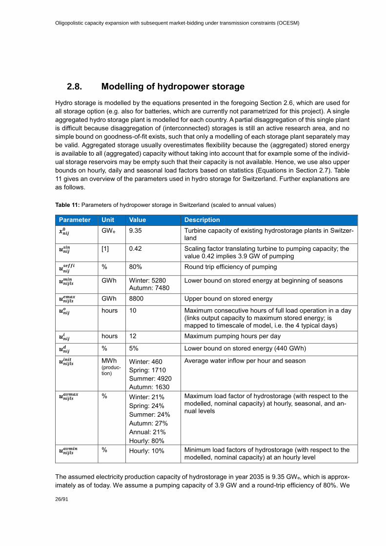
2.8. Modelling of hydropower storage
Hydro storage is modelled by the equations presented in the foregoing Section 2.6, which are used for
all storage option (e.g. also for batteries, which are currently not parametrized for this project). A single
aggregated hydro storage plant is modelled for each country. A partial disaggregation of this single plant
is difficult because disaggregation of (interconnected) storages is still an active research area, and no
simple bound on goodness-of-fit exists, such that only a modelling of each storage plant separately may
be valid. Aggregated storage usually overestimates flexibility because the (aggregated) stored energy
is available to all (aggregated) capacity without taking into account that for example some of the individ-
ual storage reservoirs may be empty such that their capacity is not available. Hence, we use also upper
bounds on hourly, daily and seasonal load factors based on statistics (Equations in Section 2.7). Table
11 gives an overview of the parameters used in hydro storage for Switzerland. Further explanations are
as follows.
Table 11: Parameters of hydropower storage in Switzerland (scaled to annual values)
Parameter Unit Value Description
𝒙𝒏𝒊𝒋𝟎 GWe 9.35 Turbine capacity of existing hydrostorage plants in Switzer-
land
𝒖𝒏𝒊𝒋𝒔𝒊𝒏 [1] 0.42 Scaling factor translating turbine to pumping capacity; the
value 0.42 implies 3.9 GW of pumping
𝒖𝒏𝒊𝒋𝒔𝒆𝒇𝒇𝒊
% 80% Round trip efficiency of pumping
𝒖𝒏𝒊𝒋𝒍𝒔𝒎𝒊𝒏 GWh Winter: 5280
Autumn: 7480 Lower bound on stored energy at beginning of seasons
𝒖𝒏𝒊𝒋𝒍𝒔𝒆𝒎𝒂𝒙 GWh 8800 Upper bound on stored energy
𝒖𝒏𝒊𝒋𝒐 hours 10 Maximum consecutive hours of full load operation in a day
(links output capacity to maximum stored energy; is mapped to timescale of model, i.e. the 4 typical days)
𝒖𝒏𝒊𝒋𝒊 hours 12 Maximum pumping hours per day
𝒖𝒏𝒊𝒋𝒅 % 5% Lower bound on stored energy (440 GWh)
𝒖𝒏𝒊𝒋𝒍𝒔𝒊𝒏𝒊𝒕 MWh
(produc-tion)
Winter: 460
Spring: 1710
Summer: 4920
Autumn: 1630
Average water inflow per hour and season
𝒖𝒏𝒊𝒋𝒍𝒔𝒂𝒗𝒎𝒂𝒙 % Winter: 21%
Spring: 24%
Summer: 24%
Autumn: 27%
Annual: 21%
Hourly: 80%
Maximum load factor of hydrostorage (with respect to the modelled, nominal capacity) at hourly, seasonal, and an-nual levels
𝒖𝒏𝒊𝒋𝒍𝒔𝒂𝒗𝒎𝒊𝒏 % Hourly: 10% Minimum load factors of hydrostorage (with respect to the
modelled, nominal capacity) at an hourly level
The assumed electricity production capacity of hydrostorage in year 2035 is 9.35 GWe, which is approx-
imately as of today. We assume a pumping capacity of 3.9 GW and a round-trip efficiency of 80%. We
27/91
do not allow pumping to occur more than 12 hours in a day, which means that currently pumping in the
model is used for daily cycles (we do not model week-ends in this project).
The assumed water storage volume is 8.8 TWh (in units of electricity production). The aggregated
hydrostorage plant can operate at full load (100%) for at most 10 consecutive hours in a typical day
(8.8/9.35*4/365*1000 = 10.3 hours). This number of hours is given as a constraint in the model because
it relates water volume to output capacity, which is relevant for (occasional) capacity expansion.
In order to be consistent with the statistics, we force a minimum amount of water to be available at the
beginning of each annual cycle (otherwise the aggregation of the hydrostorage plants could
overestimate the flexibility and result in less available water in the beginning of winter than historically
observed); we set that in the first hour of winter the total amount of water in all Swiss reservoirs to be at
least 5280 GWh (or 60% of the maximum the stored energy). Also, due to the time-scale aggregation to
a single typical day per season, we set a constraint at the beginning of the typical day of autumn on the
minimum storage volume (about 85% of maximum stored energy). This lower bound is required not to
extensively empty the reservoirs during summer. Finally, we introduce a constraint that maintains a min-
imum level of water into the reservoirs at 5% of the stored capacity to avoid complete emptying reser-
voirs in spring (depth of discharge).
The water inflows are exogenously given in each season by historically averaged (2010-2015), aggre-
gated inflows. The water inflow is constant in each hour of the typical day per season. Consistent with
the observed water inflow patterns, highest inflow occurs in the typical day of summer, while the lowest
inflow in the typical day of winter.
The additional load factors of hydrostorage capacity are necessary because of both plant aggregation
and time-scale aggregation. Currently the model parameterizes the load factors of the year 2016 to be
consistent with the statistics of the model’s calibration year, and these rates are kept unchanged in the
future (alternatively one could argue to use historical load factors over a decade or more). The load
factors are relativ to the hydrostorage capacity used in the model, which may include the capacity of
turbines that are in reality not operated because they are spare capacity or under maintenance. The
load factors are bounded from below and from above, at all time scales used in the model (i.e. hourly,
daily, seasonal, and annual) to mitigate the effects of aggregation and to be consistent with the Swiss
statistics of 2016.
Figure 5 presents the average monthly water levels (in terms of GWh electricity) in the Swiss reservoirs
in different historical years. The model result (in terms of the water level at the beginning and the end of
the typical seasonal day) are shown at the first and last month of the season. Hence, the model captures
the intra-annual pattern of the stored water and it is also close to the absolute values of stored water
observed in different seasons.

Oligopolistic capacity expansion with subsequent market-bidding under transmission constraints (OCESM)
28/91
Figure 5: Historical water levels (GWh electricity) of the years 2010–2014, and the water level as an output of the
model (thick black bars; two levels per season). The model has 4 typical days (winter, summer, fall, winter) with 24
hours each; hence, the level of hour 1 of a typical day is identified with the (real-world) water level in the first
month of the corresponding season, whereas hour 24 with the last month of the season
2.9. Numerical model solving
2.9.1. Open-Loop: PATH solver
The open loop problem is formulated as a mixed complementarity problem, which is defined as fol-
lows. Given a function 𝐹: ℜ𝑛 → ℜ𝑛and bounds 𝑙, 𝑢 ∈ ℜ𝑛, find 𝑧 ∈ ℜ𝑛 , 𝑤, 𝑣 ∈ ℜ+𝑛 :
𝐹(𝑧) = 𝑤 − 𝑣
𝑙 ≤ 𝑧 ≤ 𝑢
such that
(𝑧 − 𝑙)𝑇𝑤 = 0
(𝑢 − 𝑧)𝑇𝑢 = 0
The PATH solver is an implementation of a stabilised Newton method for solving the above mixed com-
plementarity problems. The algorithm makes use of the path construction and searching techniques first
explored by (Ralph, 1994) and later developed by (Dirkse and Ferris, 1995). The basic idea is to con-
struct a local approximation of the nonlinear equations around a given point 𝑥𝑘, solve the approximation
to find the Newton point 𝑥𝑁, update the iterate 𝑥𝑘+1 = 𝑥𝑁, and repeat until the solution to the non-linear
0
1000
2000
3000
4000
5000
6000
7000
8000
Dec Jan Feb Mar Apr May Jun Jul Aug Sep Oct Nov
En
erg
y V
olu
me
(G
Wh
)
2010
2011
2012
2013
2014
Model

29/91
system is found. This method works well close to a solution, but can fail to make progress when started
far from a solution. To guarantee progress is made, a line search between 𝑥𝑘 and 𝑥𝑁 is used to enforce
sufficient decrease on an appropriately defined merit function; typically 1
2‖𝐹(𝑥)‖2 is used. Particularly,
PATH uses a generalisation of this method on a nonsmooth reformulation of the complementarity prob-
lem. To construct the Newton direction, the normal map representation is used:
𝐹(𝜋(𝑥)) + 𝑥 − 𝜋(𝑥)
This representation is associated with the mixed complementarity problem. In the above formulation
𝜋(𝑥) is the Euclidean projection of 𝑥 in the box defined by its lower and upper bounds. A vector 𝑥 solves
the normal map representation only if 𝑧 = 𝜋(𝑥) solves an MCP.
The PATH algorithm relies on the key ideas of Newton’s method for solving a system of nonlinear equa-
tions. In the PATH solver each non-linear complementarity problem (NCP), reformulated as a normal
map, is transformed into a sequence of linear complementarity problems (LCP). In each iteration of the
algorithm, each LCP is solved by constructing first-order Taylor approximations to the functions 𝐹(𝜋(𝑥))
about the approximate solution calculated from the previous LCP. A type of damping is employed in
order to speed convergence. The bulk of computation in PATH is done in the computation of the path to
the Newton point, and more specifically in the pivotal techniques used to compute the Newton point.
2.9.2. Closed-Loop: Diagonalization
Several alternative solution methods for EPEC problems proposed in the literature were studied. It still
seems that the chosen iterative diagonalisation approach is the most robust algorithm to work with real-
world numerical data. The solution is obtained in three steps:
1. Solve the (simple) social welfare-maximisation problem. Use the obtained solution as a starting
solution for 2.
2. Solve the open-loop model (investment and production are decided in a single decision, i.e. single
step modelling). Use the obtained optimal solution as starting solution for 3.
3. Solve the (two-stage) EPEC with a diagonalisation technique across the players. That is, each
player solves subsequently an MPEC, given the fixed decisions of the other players (Gauss-Seidel
type iterations).

Oligopolistic capacity expansion with subsequent market-bidding under transmission constraints (OCESM)
30/91
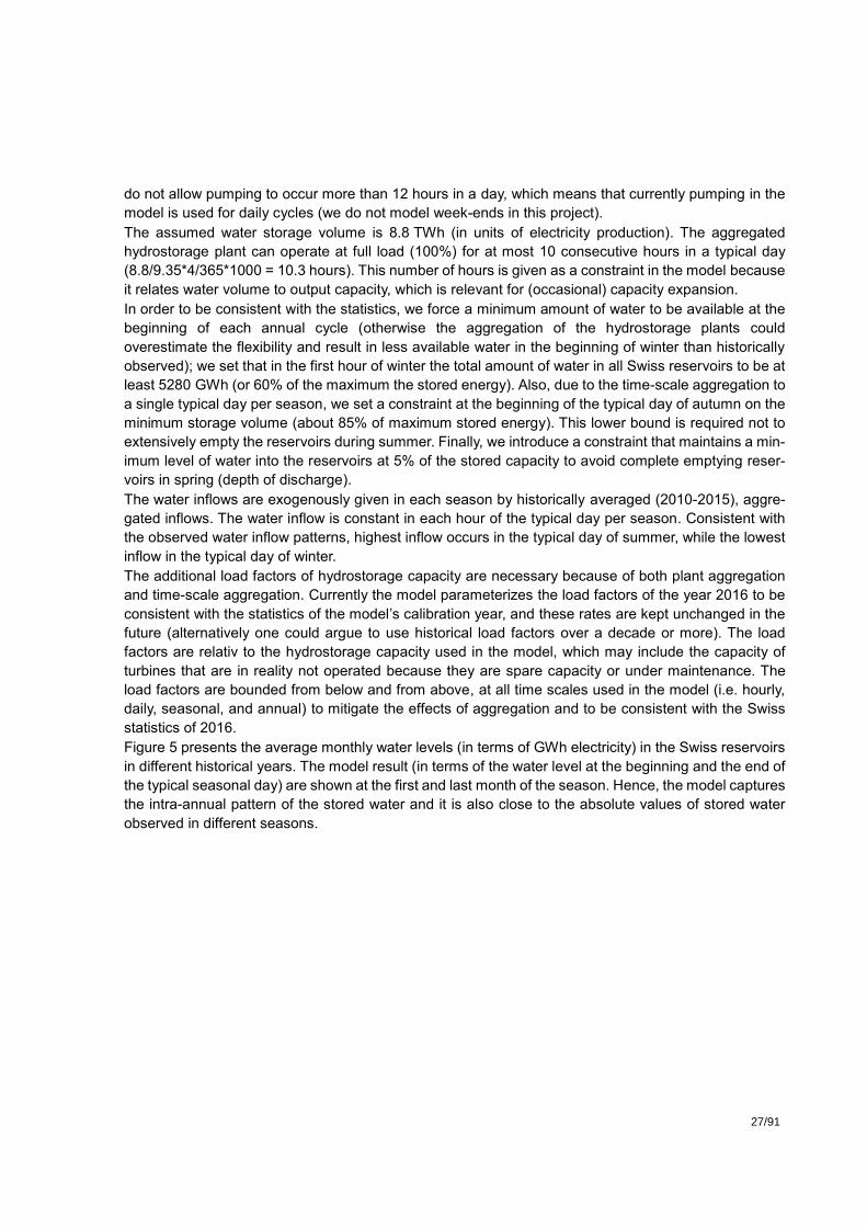
3. Data Input
Table 12 shows the major categories of data and relevant literature references. The authors can pro-
vide the full data-input spreadsheet upon request.
Table 12: Data sets used in the market model for the “today” scenario (see the section on scenario definitions for
scenario-specific values)
Type Description Year Data source
Capacity per
plant type
Nominal capacity of power plants in AT, DE,
FR, IT, and CH
2015 ENTSO-E, OECD –
Eurostat, E-control
Austria, Bundesnetza-
gentur, Schweizeri-
sche Elektriziätsstatis-
tik
Capacity per
plant subtype
Detailed capacity of gas and oil technolo-
gies (breakdown: combined cycle, gas tur-
bine, steam turbine)
2011 Elmod (European elec-
tricity model), main-
tained by TU Berlin
Production /
Availability
factors of re-
newables
Production vs capacity of intermittent re-
newables (Availability factors)
2013 OECD – Eurostat; EU
Trends Scenarios: cur-
rent 2015 produc-
tion/capacity. So-
lar/wind: ENTSO-E
Technical
availability
Availability factors of non-renewable plants 2011 DIW (Schröder, 2013),
and historical esti-
mates based on EN-
TSO-E and EU-Trends
data
Potential Technical potential of renewable technolo-
gies under socio-economic constraints
2013 JRC
CAPEX Capital costs, lifetime of generation technol-
ogies (discount rate = 5%, parameterizable)
2010 DIW (Schröder, 2013)
VAROM Variable Operation & Maintenance costs 2010 DIW (Schröder, 2013)
FIXOM Fixed Operation & Maintenance costs 2010 DIW (Schröder, 2013)
Efficiency Energy efficiency of technology and effi-
ciency loss by part-load operation
2010 DIW (Schröder, 2013)
Fuel price Gas, Oil, Coal (without CO2 price). 2015/16 (av-
erage values)
Energate messenger:
Coal index (avg.
2015/16), Gas: TTF
spot; Oil: DIW (Schrö-
der, 2013)
CO2 price 5 EUR/tCO2 2016 (approx-
imate average
value)
EEX

31/91
Price / Vol-
umes
Day-ahead cleared volumes and prices 2015 EPEX/GME
Load Load per country (incl. transmission losses,
net pumping); externally given. For exam-
ple, the future load is scenario dependent.
The load value is iteratively matched
through successive model runs by adjusting
the day-ahead volume such that (approxi-
mately): Load = Day-ahead volume +
(Amount that this not marketed day-ahead)
2015 ENTSO-E
Day-ahead
elasticities of
demand-bids
Volume elasticities of the day-ahead market
for different load periods
2015 EPEX (bid- and ask
curves); estimated in
the master thesis (C.
Groh)
Solar and
wind profiles
Hourly wind and solar generation profiles
for the countries
2015 ENTSO-E
Transmission
capacities
Aggregated line capacities between coun-
tries, based on the NTC values
2015/16 ENTSO-E
The following generation technologies are incorporated in the model:
Lignite power plant
Coal (anthracite) power plant
Oil-fired steam turbine
Oil combustion turbine
Oil combined-cycle turbine
Gas-fired steam turbine
Gas combustion turbine
Gas combined-cycle turbine
Nuclear plants
Biomass (includes waste and biogas)
Hydro Run-of-River
Hydro Dam (includes pumped-storage)
Wind (only onshore, because offshore technical potential is relatively low, even in the German
region; in the model, wind load factors in German are scaled-up to take into account off-shore
wind)
Solar PV (without solar thermal power, which is negligible today and is likely not cost-effective
in Europe in the future)
Some technologies are currently excluded because today’s deployment is very low and their potential
is foreseen to stay low or is very uncertain: Tidal power generation and geothermal power. Coal gasifi-
cation is also excluded because the authors believe that the technology characteristics in terms of cost
competitiveness (higher efficiency versus higher CAPEX) makes this technology comparable to conven-
tional coal technology (supercritical), which is represented in market model.
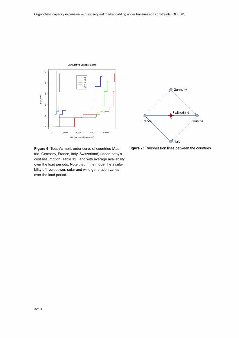
Oligopolistic capacity expansion with subsequent market-bidding under transmission constraints (OCESM)
32/91
Figure 6: Today’s merit-order curve of countries (Aus-
tria, Germany, France, Italy, Switzerland) under today’s
cost assumption (Table 12), and with average availability
over the load periods. Note that in the model the availa-
bility of hydropower, solar and wind generation varies
over the load period.
Figure 7: Transmission lines between the countries
02
04
06
08
01
00
Cumulative variable costs
MW (avg. available capacity)
EU
R/M
Wh
0 20000 40000 60000 80000
AT
DE
FR
IT
CH

33/91
4. Calibration (Scenario “today”)
Transparency measures imposed by regulators reduce the possibility to exert market power on whole-
sale power markets; market power may be defined as the deliberate back-holding of generation capacity
to yield a market price higher than the marginal cost implied by the merit-order curve (Cournot, 1838).
Price effects induced by deliberately induced market power and induced by other scarcity effects are
usually indistinguishable. For example, the temporary nuclear shut-down in France in fall 2016, which
resulted in high prices, was induced by the French nuclear regulator. A common term is the “turnkey that
was let fallen by chance by an operator into the turbine” to symbolise the indistinguishability of deliberate
market power and random effects on the supply side. Hence, we use the term “as-if” market power for
any effect that causes price deviation from the merit-order curve. Note that the “as-if” market power
cannot usually be estimated as an average deviation (Corts, 1999). Hence, it must be determined in
each load period separately to capture the idiosyncratic market situation of a particular hour (see Table
13). The employed market model is a classical Nash-Cournot model, which has an additional term of
price influence in the derivative of the objective function of each player to yield the optimality conditions
of a player. This additional price-influence term in is specifically scaled for each load period.
Table 13: Market model in estimation mode and in normal mode
The result of the estimation is shown in Figure 8, which depicts the scaled deviation between the mod-
elled merit-order curve (with all its inevitable simplifications) and the historical data of the years 2015
and 2016 as an average over each season and hour of day. In Nash-Cournot models, the deviation is
measured in terms of the “market-power” parameter θ, which is defined as θ = (p-c)/s/qTot, where p is
the current price on a market in a node, c the current marginal cost of a marginal technology (= not fully
producing technology, i.e. not bounded), s is the slope of the inverse linear demand function, and qTot is
the total quantity currently produced for a market in node (see e.g. Lagarto, 2014, where θ is sign-
reversed to our definition). The key feature of market model is that θ is not calculated outside of the
model, but with the market model itself, such that consistency is insured. For example, because the
marginal technology may not always be unambiguously determined in a multi-node model even under
perfect competition (Chen, 2008), but at least the consistency with the market model is neverhteless
ensured by using the model itself for calibration. In Figure 8, Switzerland has higher values in winter and
fall than in summer and spring, reflecting the empirical fact that in winter Switzerland’s prices are more
driven by the high prices in Italy. Germany has low values, which indicates that German prices are near
the marginal costs. The marginal costs for Germany that are relevant for the market price are in fact
challenging to estimate because the exact actual cost of coal production is publically unknown except
Estimation mode:
Input: Hourly historical prices,
market volumes, generation (for each country)
Calibration of «as-if» market power parameter (for each country and representa-tive load period)
Scaling parameter of “as-if” market power Nash-Cournot model-ling
Normal mode:
Output: prices, vol-
umes, generation by technology

Oligopolistic capacity expansion with subsequent market-bidding under transmission constraints (OCESM)
34/91
for the CO2 price, and data on the shares of wind and solar power that enter specifically the day-ahead
market is also not fully publically available.
Figure 8: Output of market model in estimation mode: Deviation between observed prices in 2015
and 2016 and the merit-order cost curve in the market model, per country (AT, DE, FR, IT, CH) and
hour of day per season (WI, SP, SU, FA).
The market structure parameter θ is determined with the market model in estimation mode for each
typical hour of each season for each country for the years 2015 and 2016.It is important to recall the
general assumptions in Section 2.2: We assume that the share of the day-ahead market volume with
respect to load stays approximately the same in the future as of today, which is related to the following
assumption on the parameter θ.
While the parameter θ is different over load periods and countries, θ is assumed to be constant over
time. In other words, because θ measures the (volume-scaled) deviation of price from the cost-merit-
order curve, we assume that the (scaled) deviations are the same in the future as of today. Because we
assume also that the share of the day-ahead market of load stays constant (see above), we assume in
total that today’s day-ahead market will have the same relevance as of today and the response of the
market to scarcity situations stays the same. Only under these two assumptions we can make quantita-
tive statements about future prices. For example, if θ would increase, we would implicitly assume that
scarcity situations on the markets leading to price peaks would increase. On the other hand, it is difficult
to estimate whether scarcity situations will be more frequent because there may be many (partially off-
setting) factors: More intermittent supply, but better demand and intermittent supply forecast, more anon-
ymous traders, but more transparency measures etc. Note also that θ measures just deviations (we
cannot detect whether this is caused by market power or any other scarcity effect) and that θ is aggre-
gated on country-level (such that specific future changes in power producing utilities may not have a
major influence). In summary, by assuming a constant θ over time, we try to take a neutral position (“as
of today”) about the target year 2035 in the investigated scenarios.
Moreover, we assume that the elasticity of demand-bids on the day-ahead market is constant over time
with the exception of the scenario “CO2+Elast”, where the elasticity is increased.
In estimation mode, the capacities of today 2015/16 are input into the model, and the 8760 + 8784 hours
of the years 2015/16 are evaluated separately with the country-specific hourly generation, hourly load,

35/91
and hourly wind and solar generation. Hence, the parameter θ is estimated separately for each hour.
Then the parameter is averaged for each season and each day-hour for the 4*24 = 96 load periods of
the market model (Figure 8). Figure 9 – Figure 13 show the historical prices together with the prices
obtained with the market model “as of today”, that is for the estimation of the years 2015 and 2016 and
the data of Table 12. For the current results, the authors still applied some additional scaling to θ to
achieve the price results, but we expect that such scaling is no longer be required when marginal cost
estimates and data quality improves (e.g. it is still difficult to obtain for the year 2016 reliable hourly
production data for Austria, but it seems that the Austrian TSO starts to publish hourly data for 2017).
Figure 9: Calibration results for Switzerland. Blue lines: EPEX price range 2015+2016 repre-
sented by hourly mean ± standard deviation. Red line: Results of market model, based on the
calibrated market-structure parameter
Figure 9 shows the calibration results for Switzerland for the typical hours of the four seasons. Note that
the historical mean price curve over a day is never an actually realised curve, and the daily curves have
usually a higher variation than the curve of mean prices (see also Figure 15). The model is able to better
replicate the average price levels of spring and summer than for fall and winter in Switzerland; one
reason is that the model calibrates in its current version to the so-called PUN price of Italy, which is
010
30
50
70
Price (Switzerland, winter)
hour of day
price (
EU
R/M
Wh)
1 3 5 7 9 12 15 18 21 24
price of model
avg. price EPEX
010
20
30
40
50
Price (Switzerland, spring)
hour of day
price (
EU
R/M
Wh)
1 3 5 7 9 12 15 18 21 24
price of model
avg. price EPEX
010
20
30
40
Price (Switzerland, summer)
hour of day
price (
EU
R/M
Wh)
1 3 5 7 9 12 15 18 21 24
price of model
avg. price EPEX
020
40
60
Price (Switzerland, fall)
hour of day
price (
EU
R/M
Wh)
1 3 5 7 9 12 15 18 21 24
price of model
avg. price EPEX
Switzerland, today

Oligopolistic capacity expansion with subsequent market-bidding under transmission constraints (OCESM)
36/91
some kind of average price, whereas export and import may pay a different price, and Switzerland’s
winter prices are closer to Italian prices than in summer (this will be addressed in a forthcoming version
of the model). Indeed, by numerical experiments of parameter variations, it was found that the Swiss
price in winter is highly dependent on the Italian price, and the only means to get higher prices in Swit-
zerland in the current version of the model was to increase the original value of the variable O&M costs
for Italy, such that also the Italian price levels (in terms of PUN price) match better historical values.
Figure 10: Calibration results for Germany. Blue lines: EPEX price range 2015+2016 represented
by hourly mean ± standard deviation. Red line: Results of market model, based on the calibrated
market-structure parameter.
Figure 10 shows the relatively precise price output of the market model for Germany. It seems that the
price and generation structure in Germany is less influenced by the other countries, such that the cost
of the generation structure, which is captured by the parameter θ, is able to explain prices better com-
pared to other countries.
010
20
30
40
50
60
Price (Germany, winter)
hour of day
price (
EU
R/M
Wh)
1 3 5 7 9 12 15 18 21 24
price of model
avg. price EPEX
010
20
30
40
50
Price (Germany, spring)
hour of day
price (
EU
R/M
Wh)
1 3 5 7 9 12 15 18 21 24
price of model
avg. price EPEX
010
20
30
40
Price (Germany, summer)
hour of day
price (
EU
R/M
Wh)
1 3 5 7 9 12 15 18 21 24
price of model
avg. price EPEX
010
20
30
40
50
Price (Germany, fall)
hour of day
price (
EU
R/M
Wh)
1 3 5 7 9 12 15 18 21 24
price of model
avg. price EPEX
Germany, today
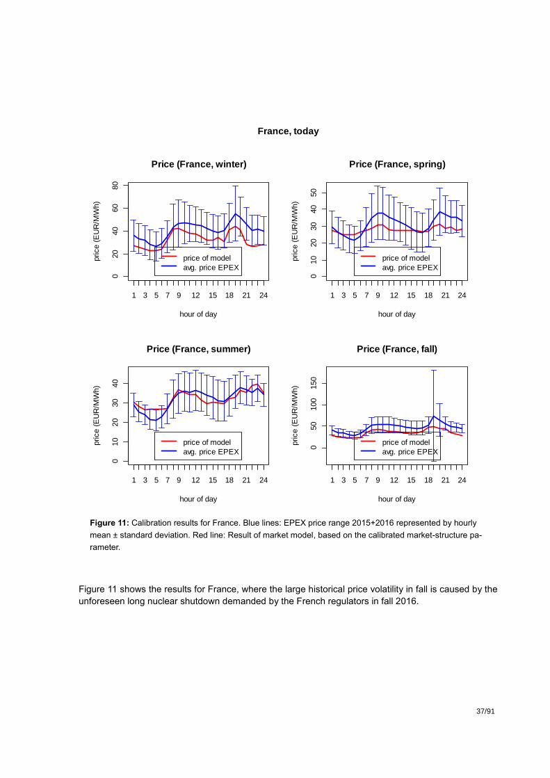
37/91
Figure 11: Calibration results for France. Blue lines: EPEX price range 2015+2016 represented by hourly
mean ± standard deviation. Red line: Result of market model, based on the calibrated market-structure pa-
rameter.
Figure 11 shows the results for France, where the large historical price volatility in fall is caused by the
unforeseen long nuclear shutdown demanded by the French regulators in fall 2016.
020
40
60
80
Price (France, winter)
hour of day
price (
EU
R/M
Wh)
1 3 5 7 9 12 15 18 21 24
price of model
avg. price EPEX
010
20
30
40
50
Price (France, spring)
hour of day
price (
EU
R/M
Wh)
1 3 5 7 9 12 15 18 21 24
price of model
avg. price EPEX
010
20
30
40
Price (France, summer)
hour of day
price (
EU
R/M
Wh)
1 3 5 7 9 12 15 18 21 24
price of model
avg. price EPEX
050
100
150
Price (France, fall)
hour of day
price (
EU
R/M
Wh)
1 3 5 7 9 12 15 18 21 24
price of model
avg. price EPEX
France, today
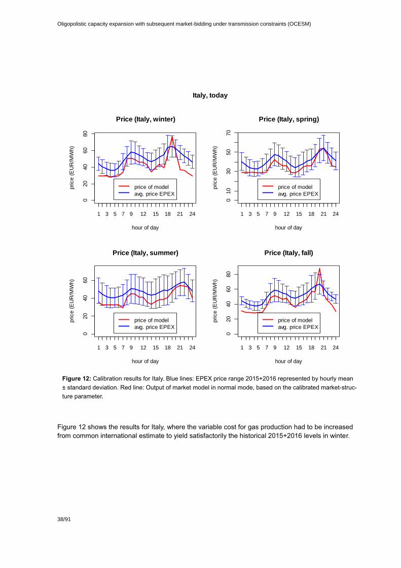
Oligopolistic capacity expansion with subsequent market-bidding under transmission constraints (OCESM)
38/91
Figure 12: Calibration results for Italy. Blue lines: EPEX price range 2015+2016 represented by hourly mean
± standard deviation. Red line: Output of market model in normal mode, based on the calibrated market-struc-
ture parameter.
Figure 12 shows the results for Italy, where the variable cost for gas production had to be increased
from common international estimate to yield satisfactorily the historical 2015+2016 levels in winter.
020
40
60
80
Price (Italy, winter)
hour of day
price (
EU
R/M
Wh)
1 3 5 7 9 12 15 18 21 24
price of model
avg. price EPEX
010
30
50
70
Price (Italy, spring)
hour of day
price (
EU
R/M
Wh)
1 3 5 7 9 12 15 18 21 24
price of model
avg. price EPEX
020
40
60
Price (Italy, summer)
hour of day
price (
EU
R/M
Wh)
1 3 5 7 9 12 15 18 21 24
price of model
avg. price EPEX
020
40
60
80
Price (Italy, fall)
hour of day
price (
EU
R/M
Wh)
1 3 5 7 9 12 15 18 21 24
price of model
avg. price EPEX
Italy, today

39/91
Figure 13: Calibration results for Austria. Blue lines: EPEX price range in years 2015/16 represented by
hourly mean +/- standard deviation. Red line: Output of market model in normal mode, based on the cali-
brated market-structure parameter.
Figure 13 shows the calibration result for Austria, which is an artificial result because currently Ger-
many and Austria belong to the same EPEX market zone.
010
20
30
40
50
60
Price (Austria, winter)
hour of day
price (
EU
R/M
Wh)
1 3 5 7 9 12 15 18 21 24
price of model
avg. price EPEX
010
20
30
40
50
Price (Austria, spring)
hour of day
price (
EU
R/M
Wh)
1 3 5 7 9 12 15 18 21 24
price of model
avg. price EPEX
010
20
30
40
Price (Austria, summer)
hour of day
price (
EU
R/M
Wh)
1 3 5 7 9 12 15 18 21 24
price of model
avg. price EPEX
010
20
30
40
50
Price (Austria, fall)
hour of day
price (
EU
R/M
Wh)
1 3 5 7 9 12 15 18 21 24
price of model
avg. price EPEX
Austria, today

Oligopolistic capacity expansion with subsequent market-bidding under transmission constraints (OCESM)
40/91
Figure 14: Comparison of alternative, simpler model formulations in case of Germany. Blue lines: EPEX price
range winter 2015+2016 represented by hourly mean +/- standard deviation. Red/orange line: Social welfare
maximisation without/with thermal dispatch constraints. Black/green line: Market model without/with thermal dis-
patch constraints. Right: Additionally, the prices of the first 60 days of winter 2015 superimposed
A major feature of the market model in comparison to traditional models is to capture price levels and
price volatility, whereas traditional central planner (= social welfare = perfect competition) models can
only capture marginal costs, or can only produce prices by adding a mark-up. Notwithstanding, the
market model also adds some markup to the marginal costs, but this markup (parameter θ) is directly
linked to the scarcity of supply, which is the main factor that drives prices up, independent whether the
scarcity is induced deliberately or not. Figure 14 compares the marginal costs (prices) obtained with the
market model in social-welfare mode (θ = 0) with the usual mode (θ <> 0) for the example of Germany.
In addition, in separate model runs–-both for the social-welfare maximisation as well as for the normal
game-theoretic mode of the model–-the technical constraints for thermal generation are switched off.
Apparently, the marginal costs by social welfare maximisation are rather flat over the day, and cannot
capture the pattern of real electricity prices; the marginal cost is just the variable cost of the marginal
technology which usually does not frequently vary over the day. Note that in the model, we use a sim-
plified merit-order curve aggregated by plant type having only a few steps, whereas in reality the merit-
order curve is nearly continuous if each individual plant’s different variable cost is taking into account.
Nevertheless, this may not be sufficient to model price peaks in certain scarcity situations. On the other
hand, taking into account the technical dispatch constraints for thermal generation improves the varia-
bility of the prices even in case of an aggregated merit order curve; Figure 15 shows similar results for
Switzerland.
01
02
03
04
05
06
0
Price (Germany, winter)
hour of day
pri
ce
(E
UR
/MW
h)
1 2 3 4 5 6 7 8 9 11 13 15 17 19 21 23
social welfare, no dispatch constraints
social welfare, with dispatch constraints
BEM model, no dispatch constraints
BEM model, with dispatch constraints
seasonal avg. price 2015/16 (+/-SD)

41/91
Figure 15: Comparison of alternative, simpler model formulations for Switzerland. Blue lines: EPEX price range
2015+2016 represented by hourly mean ± standard deviation. Red/orange line: Social welfare maximisation
without/with thermal dispatch constraints. Black/green line: Market model without/with thermal dispatch con-
straints Right: Additionally, the prices first 60 days of summer 2015 superimposed.
As mentioned, one of the goals of the market model is to capture price volatility. Table 14 shows the
volatility of hourly price returns (logarithm of price), historically for the years 2015+2016 and in the model.
For example, the column “DE/winter” in Table 14 corresponds to the prices of the market model in Figure
14. Noteworthy is the historically high volatility, which can also be seen in Figure 14. According to the
table, the market model cannot capture such very high volatilities, but can better represent the price
volatility of a typical day than a social welfare maximisation model.
01
02
03
04
05
0
Price (Switzerland, summer)
hour of day
pri
ce
(E
UR
/MW
h)
1 2 3 4 5 6 7 8 9 11 13 15 17 19 21 23
social welfare, no dispatch constraints
social welfare, with dispatch constraints
BEM model, no dispatch constraints
BEM model, with dispatch constraints
seasonal avg. price 2015/16 (+/-SD)

Oligopolistic capacity expansion with subsequent market-bidding under transmission constraints (OCESM)
42/91
Table 14: Examples of price volatility in model and historical volatility. Volatility of price = sd (log price)
Model Type Volatility of electricity price
Winter Summer
DE CH DE CH
Social welfare maximization, without dispatch constraints 0% 1% 0% 0%
Social welfare maximization, with dispatch constraints 6% 4% 4% 3%
Market model, without dispatch constraints 11% 11% 8% 8%
Market model, with dispatch constraints 16% 15% 9% 9%
Historical Benchmark, year 2015 + 16 45% 9% 15% 12%
Figure 16: Above: Average yearly and average seasonal hourly trade (MW) of the calibration run of
the market model (scenario “today”). Below: Historical yearly average trade pattern 2016 (MW). The
greyed arrows are the aggregated line constraints, and dark orange colour means more utilisation of
transmission capacity
Unlike the majority of other models that impose today’s trade amounts as a constraint in the modelled
base year, such that today’s trading pattern is trivially matched by the model, the market model also
tries to replicate today’s trades (at least approximately) endogenously. Figure 16 shows the result of the
model run. At the moment, we cannot yet replicate the large amount of transit from Germany to Italy, but
we can capture most of the signs and the order of magnitudes correctly.
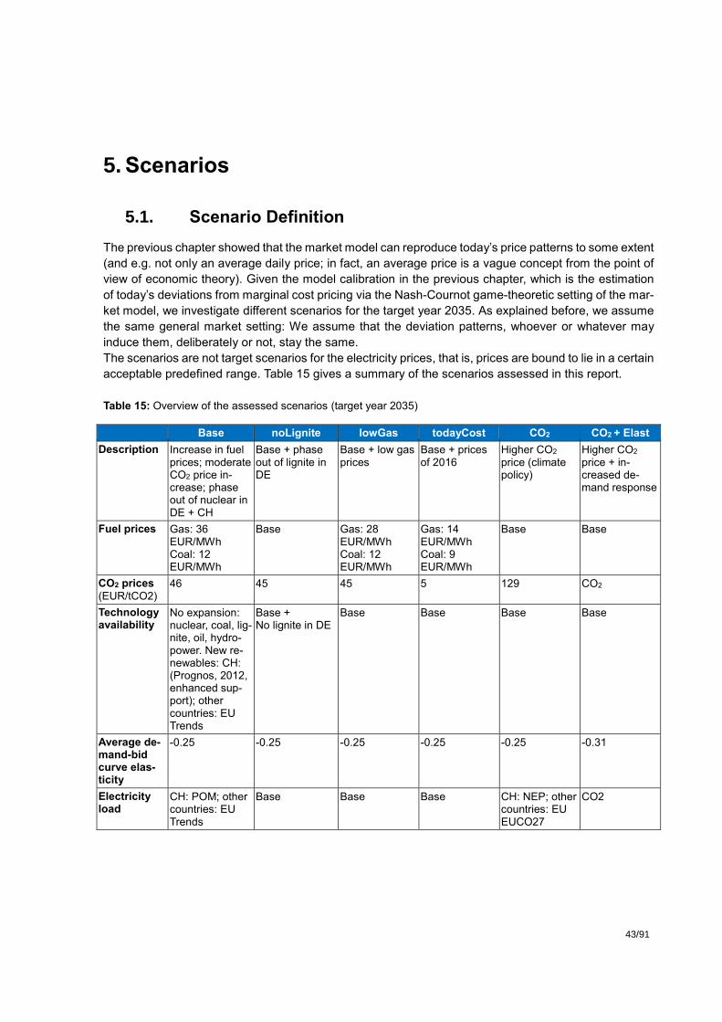
43/91
5. Scenarios
5.1. Scenario Definition
The previous chapter showed that the market model can reproduce today’s price patterns to some extent
(and e.g. not only an average daily price; in fact, an average price is a vague concept from the point of
view of economic theory). Given the model calibration in the previous chapter, which is the estimation
of today’s deviations from marginal cost pricing via the Nash-Cournot game-theoretic setting of the mar-
ket model, we investigate different scenarios for the target year 2035. As explained before, we assume
the same general market setting: We assume that the deviation patterns, whoever or whatever may
induce them, deliberately or not, stay the same.
The scenarios are not target scenarios for the electricity prices, that is, prices are bound to lie in a certain
acceptable predefined range. Table 15 gives a summary of the scenarios assessed in this report.
Table 15: Overview of the assessed scenarios (target year 2035)
Base noLignite lowGas todayCost CO2 CO2 + Elast
Description Increase in fuel prices; moderate CO2 price in-crease; phase out of nuclear in DE + CH
Base + phase out of lignite in DE
Base + low gas prices
Base + prices of 2016
Higher CO2 price (climate policy)
Higher CO2 price + in-creased de-mand response
Fuel prices Gas: 36 EUR/MWh Coal: 12 EUR/MWh
Base Gas: 28 EUR/MWh Coal: 12 EUR/MWh
Gas: 14 EUR/MWh Coal: 9 EUR/MWh
Base Base
CO2 prices
(EUR/tCO2) 46 45 45 5 129 CO2
Technology availability
No expansion: nuclear, coal, lig-nite, oil, hydro-power. New re-newables: CH: (Prognos, 2012, enhanced sup-port); other countries: EU Trends
Base + No lignite in DE
Base Base Base Base
Average de-mand-bid curve elas-ticity
-0.25 -0.25 -0.25 -0.25 -0.25 -0.31
Electricity load
CH: POM; other countries: EU Trends
Base Base Base CH: NEP; other countries: EU EUCO27
CO2
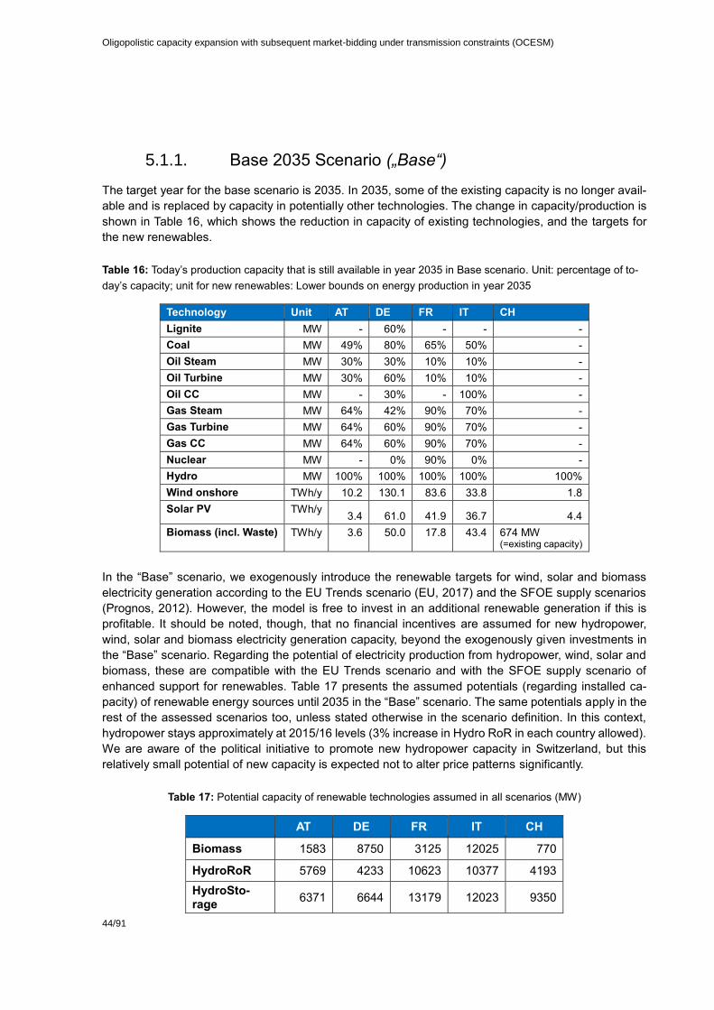
Oligopolistic capacity expansion with subsequent market-bidding under transmission constraints (OCESM)
44/91
5.1.1. Base 2035 Scenario („Base“)
The target year for the base scenario is 2035. In 2035, some of the existing capacity is no longer avail-
able and is replaced by capacity in potentially other technologies. The change in capacity/production is
shown in Table 16, which shows the reduction in capacity of existing technologies, and the targets for
the new renewables.
Table 16: Today’s production capacity that is still available in year 2035 in Base scenario. Unit: percentage of to-
day’s capacity; unit for new renewables: Lower bounds on energy production in year 2035
Technology Unit AT DE FR IT CH
Lignite MW - 60% - - -
Coal MW 49% 80% 65% 50% -
Oil Steam MW 30% 30% 10% 10% -
Oil Turbine MW 30% 60% 10% 10% -
Oil CC MW - 30% - 100% -
Gas Steam MW 64% 42% 90% 70% -
Gas Turbine MW 64% 60% 90% 70% -
Gas CC MW 64% 60% 90% 70% -
Nuclear MW - 0% 90% 0% -
Hydro MW 100% 100% 100% 100% 100%
Wind onshore TWh/y 10.2 130.1 83.6 33.8 1.8
Solar PV TWh/y 3.4 61.0 41.9 36.7 4.4
Biomass (incl. Waste) TWh/y 3.6 50.0 17.8 43.4 674 MW (=existing capacity)
In the “Base” scenario, we exogenously introduce the renewable targets for wind, solar and biomass
electricity generation according to the EU Trends scenario (EU, 2017) and the SFOE supply scenarios
(Prognos, 2012). However, the model is free to invest in an additional renewable generation if this is
profitable. It should be noted, though, that no financial incentives are assumed for new hydropower,
wind, solar and biomass electricity generation capacity, beyond the exogenously given investments in
the “Base” scenario. Regarding the potential of electricity production from hydropower, wind, solar and
biomass, these are compatible with the EU Trends scenario and with the SFOE supply scenario of
enhanced support for renewables. Table 17 presents the assumed potentials (regarding installed ca-
pacity) of renewable energy sources until 2035 in the “Base” scenario. The same potentials apply in the
rest of the assessed scenarios too, unless stated otherwise in the scenario definition. In this context,
hydropower stays approximately at 2015/16 levels (3% increase in Hydro RoR in each country allowed).
We are aware of the political initiative to promote new hydropower capacity in Switzerland, but this
relatively small potential of new capacity is expected not to alter price patterns significantly.
Table 17: Potential capacity of renewable technologies assumed in all scenarios (MW)
AT DE FR IT CH
Biomass 1583 8750 3125 12025 770
HydroRoR 5769 4233 10623 10377 4193
HydroSto-rage
6371 6644 13179 12023 9350

45/91
WindOns-hore
7170 86549 57569 25957 2675
SolarPV 21000 209000 160000 154000 20313
Also, the “Base” scenario implements the phase-out of nuclear in Germany and Switzerland, as well as
the nuclear power capacity reduction in France. The capacity reduction in France of nuclear is according
to the EU Trends Scenario (EU, 2017). Today France has 63 GW nuclear power, and in 2035 it is antic-
ipated to be reduced to 57 GW taking into account the new unit (unit Fessenheim closes 2018, but it is
replaced by unit Flamanville 3 in 2019).
The Base scenario has bounds on new conventional capacity that can be built: It is prohibited to build
new coal and oil-fueled plants, and significant new use of gas fuel is only allowed with combined cycle
technology. Finally, Table 18 presents the assumed specific investment costs in the “Base” scenario;
these costs are the same in all scenarios assessed unless stated otherwise in the scenario definition.
Figure 17: Capacity of 2015/16 and remaining old capacity available in 2035
0
20
40
60
80
100
120
140
160
180
200
2015/16 2035
GW
Existing capacity that is still available, Germany
SolarPV
WindOnshore
HydroStorage
HydroRoR
Biomass
Nuclear
GasCC
GasTurbine
GasSteam
OilCC
OilTurbine
OilSteam
Coal
Lignite0
2
4
6
8
10
12
14
16
18
20
2015/16 2035
GW
Existing capacity that is still available, Switzerland
SolarPV
WindOnshore
HydroStorage
HydroRoR
Biomass
Nuclear
GasCC
GasTurbine
GasSteam
OilCC
OilTurbine
OilSteam
Coal
Lignite
0
20
40
60
80
100
120
140
2015/16 2035
GW
Existing capacity that is still available, France
SolarPV
WindOnshore
HydroStorage
HydroRoR
Biomass
Nuclear
GasCC
GasTurbine
GasSteam
OilCC
OilTurbine
OilSteam
Coal
Lignite 0
20
40
60
80
100
120
140
2015/16 2035
GW
Existing capacity that is still available, Italy
SolarPV
WindOnshore
HydroStorage
HydroRoR
Biomass
Nuclear
GasCC
GasTurbine
GasSteam
OilCC
OilTurbine
OilSteam
Coal
Lignite 0
5
10
15
20
25
30
2015/16 2035
GW
Existing capacity that is still available, Austria
SolarPV
WindOnshore
HydroStorage
HydroRoR
Biomass
Nuclear
GasCC
GasTurbine
GasSteam
OilCC
OilTurbine
OilSteam
Coal
Lignite
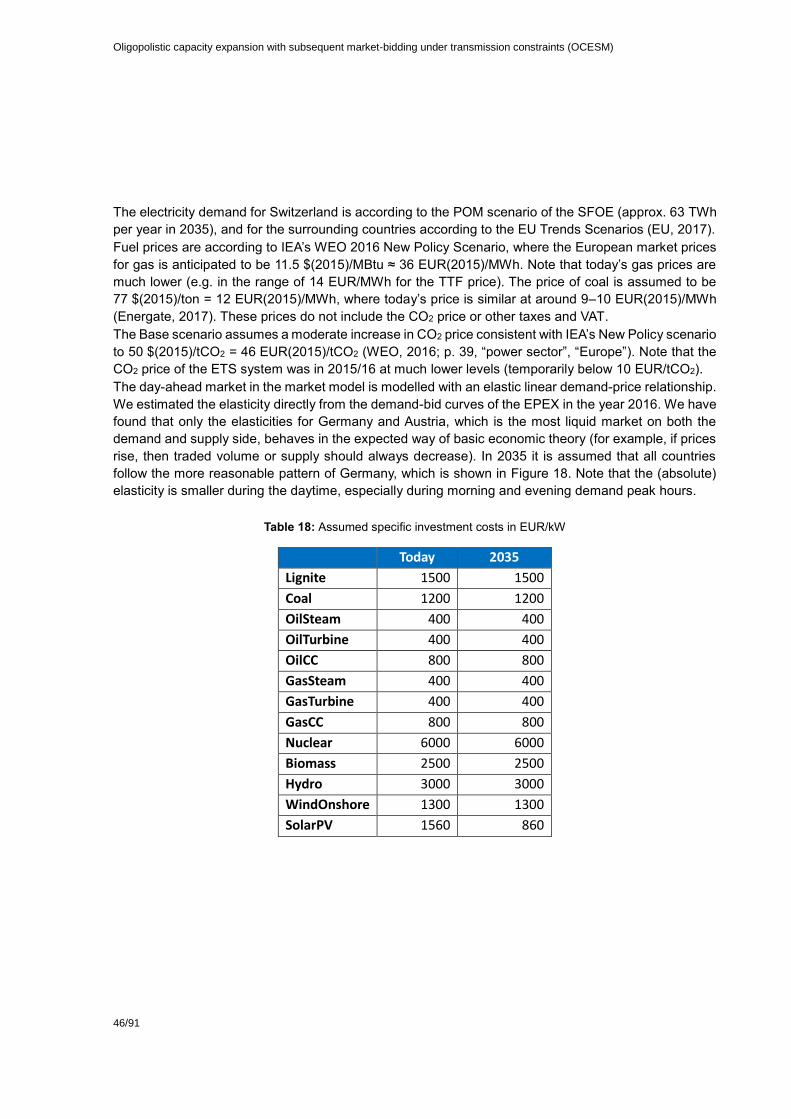
Oligopolistic capacity expansion with subsequent market-bidding under transmission constraints (OCESM)
46/91
The electricity demand for Switzerland is according to the POM scenario of the SFOE (approx. 63 TWh
per year in 2035), and for the surrounding countries according to the EU Trends Scenarios (EU, 2017).
Fuel prices are according to IEA’s WEO 2016 New Policy Scenario, where the European market prices
for gas is anticipated to be 11.5 $(2015)/MBtu ≈ 36 EUR(2015)/MWh. Note that today’s gas prices are
much lower (e.g. in the range of 14 EUR/MWh for the TTF price). The price of coal is assumed to be
77 $(2015)/ton = 12 EUR(2015)/MWh, where today’s price is similar at around 9–10 EUR(2015)/MWh
(Energate, 2017). These prices do not include the CO2 price or other taxes and VAT.
The Base scenario assumes a moderate increase in CO2 price consistent with IEA’s New Policy scenario
to 50 $(2015)/tCO2 = 46 EUR(2015)/tCO2 (WEO, 2016; p. 39, “power sector”, “Europe”). Note that the
CO2 price of the ETS system was in 2015/16 at much lower levels (temporarily below 10 EUR/tCO2).
The day-ahead market in the market model is modelled with an elastic linear demand-price relationship.
We estimated the elasticity directly from the demand-bid curves of the EPEX in the year 2016. We have
found that only the elasticities for Germany and Austria, which is the most liquid market on both the
demand and supply side, behaves in the expected way of basic economic theory (for example, if prices
rise, then traded volume or supply should always decrease). In 2035 it is assumed that all countries
follow the more reasonable pattern of Germany, which is shown in Figure 18. Note that the (absolute)
elasticity is smaller during the daytime, especially during morning and evening demand peak hours.
Table 18: Assumed specific investment costs in EUR/kW
Today 2035
Lignite 1500 1500
Coal 1200 1200
OilSteam 400 400
OilTurbine 400 400
OilCC 800 800
GasSteam 400 400
GasTurbine 400 400
GasCC 800 800
Nuclear 6000 6000
Biomass 2500 2500
Hydro 3000 3000
WindOnshore 1300 1300
SolarPV 1560 860

47/91
Figure 18: Price elasticity assumption per season, common to all countries
5.1.2. No Lignite Production Scenario (“noLignite”)
The No Lignite scenario has the same parameters as the Base Scenario except that all lignite power
plants in Germany are phased out.
5.1.3. Low Gas Price Scenario (“lowGas”)
The LowGas scenario has the same parameters as the Base Scenario except for the gas price. The gas
price is the same as today’s 2015/16 low prices, that is, approx. 14 EUR/MWh (TTF). Higher gas prices
in the power sector than in the Base scenario are likely driven entirely by the CO2 price, which is covered
by the CO2 scenario below.
5.1.4. Today’s Cost Scenario (“todayCost”)
The todayCost scenario has the same parameters as the Base Scenario except that the marginal costs
of all technologies are as of today. Hence, the variable operating costs, the fuel and CO2 prices in this
scenario as in the “today” scenario, while the existing electricity generation capacity is as in the “Base”
scenario. We keep in the “todayCost” scenario the reduction in the solar PV investment costs as in the
“Base” scenario. Since in this scenario the fuel and CO2 prices remain as of today, this implies a signif-
icant change for gas production costs compared to the “Base” and “lowGas” scenarios (see above for
gas costs in “Base” and “lowGas” scenario). In summary, “todayCost” scenario differs from the “Base”
scenario in the following::
Today’s coal prices are slightly less than in “Base” (9 EUR/MWh vs. 12 EUR/MWh).
Gas prices are less than in “Base” (14 EUR/MWh vs. 36 EUR/MWh)
-0.35
-0.30
-0.25
-0.20
-0.15
-0.10
-0.05
0.00
01 02 03 04 05 06 07 08 09 10 11 12 13 14 15 16 17 18 19 20 21 22 23 24
Ela
sti
cit
y
Winter
-0.30
-0.25
-0.20
-0.15
-0.10
-0.05
0.00
01 02 03 04 05 06 07 08 09 10 11 12 13 14 15 16 17 18 19 20 21 22 23 24
Ela
sti
cit
y
Spring
-0.40
-0.35
-0.30
-0.25
-0.20
-0.15
-0.10
-0.05
0.00
01 02 03 04 05 06 07 08 09 10 11 12 13 14 15 16 17 18 19 20 21 22 23 24
Ela
sti
cit
y
Summer
-0.40
-0.35
-0.30
-0.25
-0.20
-0.15
-0.10
-0.05
0.00
01 02 03 04 05 06 07 08 09 10 11 12 13 14 15 16 17 18 19 20 21 22 23 24
Ela
sti
cit
y
Autumn

Oligopolistic capacity expansion with subsequent market-bidding under transmission constraints (OCESM)
48/91
The CO2 price is at the levels of 2015/16 at approx. 5 EUR/tCO2 instead of 46 EUR/tCO2.
5.1.5. High CO2 Price Scenario (“CO2”)
The “CO2” scenario has the same parameters as the “Base” Scenario except for the following
changes:
The CO2 price is much higher using IEA’s WEO 450 Scenario (WEO, 2016; price for “power sec-
tor”): 140 $(2015)/tCO2 = 129 EUR(2015)/tCO2.
The demand for Switzerland is according to the NEP scenario of the SFOE (approx. 60 TWh per
year in 2035), and the demand for the surrounding countries according to EUCO 27 climate miti-
gation scenario of the EU (EU, 2016). Note that as mentioned earlier, the demand output visible
of the market model is a wholesale demand procured either domestically or by the other modelled
countries, whereas for example Germany may also procure end-use demand through other coun-
tries that are not modelled.
5.1.6. High Price-Demand Elasticity Scenario (“CO2 + Elast”)
The high demand elasticity scenario has the same parameters as the “CO2” scenario except for the
following changes.
It is expected that the high CO2 price in the CO2 Scenario implies also increased demand-side
substitution effects by decentral generation and by demand-side management (e.g. by local stor-
age of power in batteries). In this context, we assume that the demand-price elasticity is increased
by 25%.
The whole sale demands of the countries were adapted to counterbalance the demand-loss
through the higher elasticity.
Table 19: Marginal production cost (EUR/MWh) ranges (min-max) of the technologies by scenario. Source: DIW
(Schröder, 2013)
Scenario Lignite Coal Nuclear Gas CC Biomass
Today 16.78 27.3 - 31.97 17.59 27.5 - 35.75 22.56 - 29.56
Base 53.50 66.76 - 71.43 17.59 78.02 - 86.27 22.56 - 29.56
lowGas 53.50 66.76 - 71.43 17.59 41.3 - 49.55 22.56 - 29.56
CO2 123.65 134.88 - 139.55 17.59 105.89 - 114.14 22.56 - 29.56
Note that the electricity load in the “Today” and “Base” scenarios in Switzerland is calibrated to be in-
line with the developments in the POM scenario. The electricity load in the “Today” and “Base” scenario
in the neighbouring countries is calibrated to be close to the demands of the EU Trend scenario. In the
rest of the scenarios the electricity load of the “Base” is given to the model as a starting point: The model
determines a changed, optimal load based on the market equilibrium.

49/91
5.2. Scenario Results
5.2.1. Future electricity prices
Four main factors contribute to the electricity prices in the assessed scenarios (Figure 19 - Figure 23):
decommissioning of existing capacity, electricity demand, natural gas price, and penetration of intermit-
tent renewables (wind and solar PV). In the following, we provide an analysis of price developments in
the five model regions. Before that, the next note is important to judge the analysis correctly in terms of
price setting in a perfect competition formulation (i.e. social welfare maximisation) and in an oligopolistic
formulation (i.e. Nash-Cournot competition).
In a perfect competition formulation, without transmission and dispatch constraints, the last producing
unit in the merit order curve sets the price. However, when dispatch constraints are included in the
formulation, then out-of-order dispatch can occur because of the constraints. Nonetheless, in both
cases, there is a single marginal technology that sets the price, which normally strictly operates between
its lower and upper capacity bounds. However, when transmission constraints are included, then the
identification of the marginal unit that sets the price is not always well defined even under perfect com-
petition. This is because the electricity flow constraints imply that a marginal MWh of demand at a loca-
tion might be optimally met by changing several production sources at once, of which one or more could
be even decreased as demand increases in order to make more transmission capacity available (Lise
et al., 2010).
In an oligopolistic formulation with transmission and dispatching constraints, the identification of the
price setting technology is even more ambiguous than in a perfect competition specification. This is
because the players of different sizes under Cournot competition will have different marginal costs in
equilibrium and the choice of the marginal plant depends upon which player is considered. Because
these units are owned by strategic players, the electricity price in the market exceeds the marginal costs
by the amount of a “mark-up”, and also there can be multiple technologies that affect the prices and are
not operating at their full capacity. When two or more of such “marginal” units are associated with a
given price in an oligopolistic market, the overall marginal cost associated with this price could be ob-
tained as the production-weighted average variable cost of those units (Chen et al., 2008). As in the
case of the perfect competition, when transmission constraints are considered then the marginal unit for
a node could also be located in different nodes if the line connecting two regions is not congested (Lise
et al., 2010).
5.2.1.1. Switzerland
In Switzerland, the gap in the electricity supply due to the nuclear phase-out is filled by electricity imports
and increased penetration of solar PV (see also Figure 24). These changes in the Swiss electricity
supply mix turn Switzerland into a net importer of electricity. This suggest that, because of the increased
dependency on imports, the Swiss electricity price is defined more often than today by the electricity
prices in the surrounding countries.
This stronger dependence of the Swiss electricity price on cross-border market areas also implies a
stronger dependence on gas fuel prices, since gas-based generation often emerges as the marginal
electricity generation technology in the surrounding countries (see also Section 6.1). This effect is ac-
centuated by the increased correlation between the Swiss and Italian electricity prices, as Italy becomes
a supplier of electricity to Switzerland by 2035 (Figure 34). On the other hand, Switzerland exports

Oligopolistic capacity expansion with subsequent market-bidding under transmission constraints (OCESM)
50/91
hydropower to Germany at least in as much (and very likely in more) hours in all seasons as today,
especially during peak hours, to substitute Germany’s phased-out nuclear power. In this context, the
average annual electricity price in Switzerland increases in all scenarios and all seasons from today’s
levels (Figure 19), since either Switzerland imports gas-based electricity, or exports electricity at the
higher German market prices by 2035.
The Swiss electricity prices in the “Base” scenario double on average from the levels of the “Today”
scenario, and this increase is persistent across all four seasons. The increase in the Swiss prices closely
follows the increase in the gas price, since the cross-border trade defines to a large extent the Swiss
price. The correlation with the gas price arises because gas often becomes the marginal technology in
the market areas of the neighbouring countries. It should be noted that this does not necessarily imply
that Switzerland always “imports” the electricity price of Austria or Italy. Exports of Swiss hydropower to
Germany also emerge, because of the German nuclear phase-out that turns the country into a net im-
porter. Particularly in summer, when the water availability is high, the Swiss exports are higher during
the peak hours in the “Base” scenario than in the “Today” scenario (see also Section 5.2.3). In such
cases, with good resource availability and low profitability of fossil-based generation because of high
fuel or CO2 prices, Swiss hydropower becomes an important market player. It is noteworthy that the
price-differences between peak and off-peak hours are only slightly larger in the “Base” scenario com-
pared to the “Today” scenario. For example, during summer the Swiss price at the 15:00 hour is about
1/3rd of the price at 09:00 in the “Base”, which is very close to the price differences at the same hours
in the “Today” scenario. However, one could have expected more substantial differences, mainly be-
cause of the increased supply of zero (or low) marginal cost electricity in Switzerland. Indeed, the in-
creased penetration of renewables in 2035 in all countries does not push the Swiss electricity prices to
lower levels than today, even in hours when resource availability is high. This result suggests that the
fossil fuel prices define the level of the electricity price in the neighbouring countries in those hours, too.
The result could also suggest that producers in the neighbouring countries try to compensate the in-
creased gas-based generation costs during the peak hours by maintaining high prices even in those
hours when the electricity generation costs are low. Hence, such practices may also influences, via the
cross-border trade, the Swiss price.
In the “TodayCost” scenario, in which the fuel and CO2 prices remain at the levels of the “Today”
scenario, but in which the electricity generation capacity and demand developments are similar to the
“Base” scenario, the electricity prices are only 15% higher than in the “Today” scenario. This increase is
mainly driven by the structural changes in the electricity generation (i.e. phase-out of the low-cost nu-
clear generation) and the increased demand. The increase in the Swiss electricity prices is more prom-
inent during peak hours, where the Swiss hydropower exports electricity to Germany at a high price (as
in the “Base” scenario). In summary, the results of the “TodayCost” scenario suggest that if the current
fossil fuel prices and—most importantly—if the current very low CO2 prices prevail in the future, then it
is likely that prices are similar as of today, independently of the nuclear phase-out in Germany and
Switzerland and of the reduction of nuclear capacity in France.
In the “LowGas” scenario, the average Swiss electricity price, i.e. across all four seasons, is about
20% lower than in the “Base” scenario, which results in higher demand and in increased annual net
imports (see also Section 5.2.2.1). It follows that in this scenario there is a stronger dependence on
cross-border trade compared with the “Base” scenario. The Swiss electricity prices in spring, summer
and fall are lower than in the “Base” scenario, corresponding to the lower electricity production costs
from gas-fuelled power plants in the neighbouring countries which lead to lower costs of imported elec-
tricity. In these seasons, the response of the Swiss electricity price to the lower cost of natural gas is

51/91
similar to the response seen in the neighbouring countries concerning the levels in the “Base” scenario.
However, the Swiss electricity price in winter remains at the same levels as in the “Base” scenario,
contrary to the developments in the neighbouring countries, where the electricity prices are also lower
in winter compared with the “Base” scenario. Compared with the prices of the neighbouring countries in
winter, the price in Switzerland is higher than in Germany in all hours except the evening peak hours.
The Swiss price is also always higher than the Austrian electricity price; indeed, it is the highest of all
neighbouring market areas during off-peak hours. This result suggests that the cross-border trade is
setting the Swiss electricity price when the availability of water and solar is low, and the Swiss demand
is relatively inelastic (i.e. price elasticity is less than 1). In the winter peak hours, Switzerland exports
hydropower to Germany at prices close to those attained in the German market. During the off-peak
winter hours, the Swiss electricity price “decouples” from the neighbouring countries and is driven by
the domestic demand rather than the gas price (since domestic gas plants do not enter into the Swiss
electricity mix) under the limited (low water and solar availability) domestic generation capacity. Hence,
the imported electricity comes at a price similar to the levels of the “Base” scenario, resulting in approx-
imately the same demand in both scenarios during these hours. Similar findings are also valid to some
extent in the “TodayCost” scenario, but in this scenario the lower CO2 prices keep the solid-based gen-
eration in the supply mix and lead to different electricity prices across the countries.
In the “noLignite” scenario, the electricity prices in Switzerland are on average on the same level as
in the “Base” scenario, as the trade pattern between Switzerland and its neighbouring countries is not
affected by the phase-out of lignite power plants in Germany. However, during the peak hours and es-
pecially in winter and autumn, the electricity prices in Switzerland are higher than in the “Base” scenario.
During these hours, high electricity prices prevail in Germany due to the phase-out of the low-cost lignite
power plants, which provide opportunities for the Swiss producers to export at high prices to supply the
German market. As a result, the domestic prices of Switzerland are also driven upwards during these
hours.
In the “CO2” scenario, the electricity price significantly increases from the “Base” scenario in all sea-
sons reflecting the increase in the production costs from fossil-based generation, and consequently the
increased costs of imported electricity. However, during the hours around noon, the higher contribution
of solar PV in this scenario (compared with the “Base”) mitigates the price increase. Particularly during
summer hours where the electricity production from solar PV peaks, prices could be lower than in the
“Base” scenario. However, the spread in the prices between hour 08:00 and 15:00 (as well as between
hour 15:00 and 21:00) is significantly higher than the corresponding spread in the “Base” scenario. This
higher volatility of the electricity price is attributable to the larger difference in the electricity generation
costs between fossil and solar sources, which is caused by the higher CO2 prices, because also in the
scenario “CO2” the gas prices are the most important driver of price level in all countries. Finally, the
“CO2+Elast” scenario exhibits similar developments as the “CO2” scenario but with a slightly lower elec-
tricity price.
5.2.1.2. Neighbouring countries
In Germany, the nuclear-phase out drives the electricity prices upwards compared to the “today” levels,
and the electricity prices are mainly influenced by the natural gas and CO2 prices. This is supported by
the results of the “todayCost” scenario, where the electricity price is 29% higher on average than the
“Today” scenario, while the demand increases by 26%; hence in this scenario, in which the fuel prices
remain at today’s low levels, the nuclear phase-out does not cause a significant increase in the electricity
prices compared with the increase induced by higher demand. Another structural change in the German

Oligopolistic capacity expansion with subsequent market-bidding under transmission constraints (OCESM)
52/91
electricity market induced by the nuclear phase-out is the trade pattern; Germany, which is annual net
exporter as of today, becomes a net importer by 2035 (by taking into account only the modelled trade of
Germany: with France, Austria, and Switzerland). Nevertheless, the amount of imports is too small (com-
pared with the volume of the domestic generation) to have a significant impact on German prices. The
“NoLignite” scenario is here an exception: During peak hours the prices are significantly higher than in
the “Base” scenario (during off-peak hours the two scenarios have similar price levels). The high peak
prices are driven by the higher cost of imported electricity from Switzerland. Finally, the increased pen-
etration of solar PV yields lower prices at noon, and also higher hourly price differences between 08:00
and 15:00 hours, as well as between 15:00 and 21:00 hours, compared to the “today” case.
On the other hand, the electricity prices in France seem not to be much affected by the developments
in the neighbouring countries. In all scenarios, prices in France remain at approximately the same level,
which can be attributed to the low penetration of gas power in the French supply mix (all scenarios
having different gas prices have hardly no impact), and to the large share of nuclear power (the impact
of CO2 prices on electricity prices is less than in other countries). France remains a net exporter of
electricity in all scenarios, the volumes of exports increase by 2035 due to increased trade with Germany
and Switzerland. However, it should be noted that the electricity price in all scenarios is lower compared
with the “Today” scenario. This result is attributable to several reasons as follows.
One reason for the lower prices in France is the increased penetration of zero-cost electricity from wind.
In a sensitivity analysis, the deployment of wind in France is halved compared to the deployment in the
“Base” scenario. The result showed that the prices in France double from the levels in the “Today” sce-
nario. In fact, as the wind is currently treated in model as a deterministic and continuous source of
electricity supply, the increased wind penetration pushes in the merit order curve the more expensive
fossil-based generation further to the right. Moreover, in France, there is no price-setting technology
since all renewable energy sources (wind, biomass, solar, hydro) as well as nuclear power operate at
their maximally feasible load factors. However, when the amount of wind power was reduced in the
sensitivity analysis, fossil-based generation (gas and oil) emerged as a price-setting technology. This
effect is persistent across all scenarios assessed, as it is independent of the gas or CO2 prices.
Another reason for the relatively low prices is that the French electricity company (EdF) is almost a
regulatory monopoly in France. The actual prices (i.e. the blue lines in Figure 21) suggest that EdF
maybe exploit some scarcity situations with higher supply-bids, but not as much as it would if it were a
full Nash-Cournot player. In this context, the calibration of the model manages to approximate today’s
prices of France with a Cournot parameter θ less than 1. A sensitivity analysis, in which θ is set to 1
resulted in doubled prices in the “Today” scenario compared with the historical averages; it follows that
the same sensitivity produced significantly higher prices in the future years for France as well. Evidence
of limited market power of EdF due to regulation can be found also in the literature. For example, in
(Lise et al., 2010) EdF is modelled as a price taker due to an implicit “regulatory threat”, in contrast to
the firms in the fringe region which can influence prices more. Consequently, also in (Lise et al., 2010),
the resulting prices in France are lower than today’s prices (pp. 31, Fig 2). Another reason is that the
models simulates competition based on the short-run marginal costs, while in reality a price mark-up is
required in France to cover nuclear plants’ fixed costs (Chen et al., 2008).
On the other hand, the exports from France to its neighbouring countries (which have higher prices than
France) cannot drive the French prices upwards. This can be attributed to (i) the relatively low amount
of exports compared to the domestic load in France (about 10% exports), (ii) the flatter merit order curve
in France due to the future increase in wind generation, and (iii) the limited price influence capability of
EdF due to regulatory threat.
53/91
In Italy, the electricity prices are also determined by the gas and CO2 prices assumed in the different
scenarios. Due to the relatively better solar resource availability in Italy, the effect of increased electricity
supply from solar PV on prices at noon in summer is more pronounced than in the northern countries.
Though, this increases also price volatility. Italy remains the country with the highest electricity prices
among all the five countries and across all scenarios, with prices exceeding sometimes 160 EUR/MWh
under a stringent climate policy (CO2 scenario). One reason for high prices is the lower imports from
Switzerland and France in 2035: Switzerland, after the nuclear phase-out, becomes a major net importer
of electricity from France, and France exports also to Germany. In this squeezed situation, the flexibility
of Italy to mitigate the pressure on electricity prices with imports is limited in all scenarios.
Finally, in Austria, the electricity prices are closely correlated with the German electricity prices (note
that Austria and Germany are today on the EPEX market a common price zone). The phase-out of
nuclear power in both Germany and Switzerland hampers electricity imports from these countries. On
the other hand, it generates opportunities for the Austrian suppliers to export. As a result, and in combi-
nation with the increased demand, investments in gas turbines combined cycles are enabled in Austria
and gas power gains share in the electricity production mix. The increased penetration of gas power
makes the price in Austria also more vulnerable to changes in the gas and CO2 prices.
The electricity prices in all scenarios and all countries are higher than the corresponding prices in the
perfect competition solution due to the use of an oligopolistic model formulation (though not the full
amount of market power can be exerted in our differentiated model setup). In reality, such high prices
may not be realistic because they would provoke regulatory intervention and because forward contracts
could also dampen price increases. By all means, an oligopolistic formulation is a useful bounding case,
for example for examining how the presence of a carbon price could interact with oligopolistic behaviour
on power markets (Lise et al., 2010).

Oligopolistic capacity expansion with subsequent market-bidding under transmission constraints (OCESM)
54/91
Figure 19: Swiss model price, and historical price variations (blue lines correspond to the mean of the years
2015 and 2016 ± hourly standard deviation)
hour of day
price
(E
UR
/MW
h)
Price (Switzerland, winter)Price (Switzerland, winter)Price (Switzerland, winter)Price (Switzerland, winter)Price (Switzerland, winter)Price (Switzerland, winter)Price (Switzerland, winter)
2015/16 av g.
today model
Base
noLig
lowGas
today Cost
CO2
CO2+Elast
20
40
60
80
100
120
140
hour of day
price
(E
UR
/MW
h)
Price (Switzerland, spring)Price (Switzerland, spring)Price (Switzerland, spring)Price (Switzerland, spring)Price (Switzerland, spring)Price (Switzerland, spring)Price (Switzerland, spring)
2015/16 av g.
today model
Base
noLig
lowGas
today Cost
CO2
CO2+Elast
hour of day
price
(E
UR
/MW
h)
Price (Switzerland, summer)Price (Switzerland, summer)Price (Switzerland, summer)Price (Switzerland, summer)Price (Switzerland, summer)Price (Switzerland, summer)Price (Switzerland, summer)
2015/16 av g.
today model
Base
noLig
lowGas
today Cost
CO2
CO2+Elast
1 3 5 7 9 11 13 15 17 19 21 23
20
40
60
80
100
120
140
hour of day
price
(E
UR
/MW
h)
Price (Switzerland, fall)Price (Switzerland, fall)Price (Switzerland, fall)Price (Switzerland, fall)Price (Switzerland, fall)Price (Switzerland, fall)Price (Switzerland, fall)
2015/16 av g.
today model
Base
noLig
lowGas
today Cost
CO2
CO2+Elast
1 3 5 7 9 11 13 15 17 19 21 23
hour of day
price (
EU
R/M
Wh)
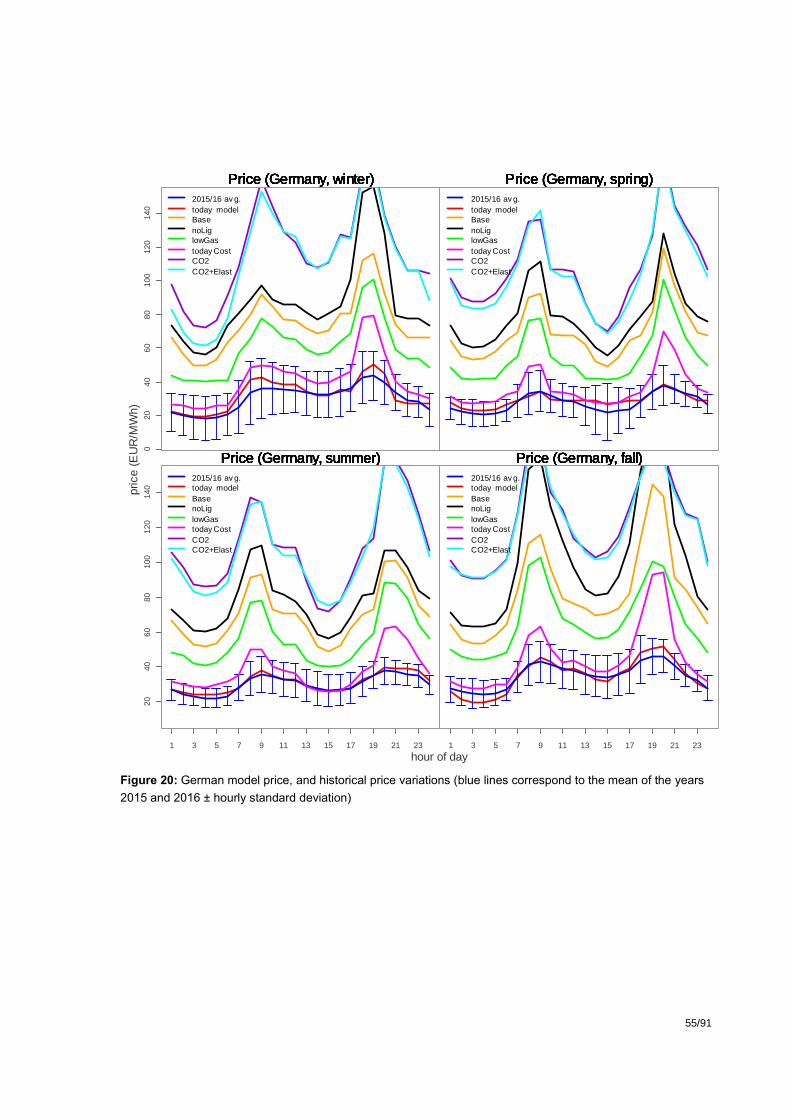
55/91
Figure 20: German model price, and historical price variations (blue lines correspond to the mean of the years
2015 and 2016 ± hourly standard deviation)
hour of day
price
(E
UR
/MW
h)
Price (Germany, winter)Price (Germany, winter)Price (Germany, winter)Price (Germany, winter)Price (Germany, winter)Price (Germany, winter)Price (Germany, winter)
2015/16 av g.
today model
Base
noLig
lowGas
today Cost
CO2
CO2+Elast
020
40
60
80
100
120
140
hour of day
price
(E
UR
/MW
h)
Price (Germany, spring)Price (Germany, spring)Price (Germany, spring)Price (Germany, spring)Price (Germany, spring)Price (Germany, spring)Price (Germany, spring)
2015/16 av g.
today model
Base
noLig
lowGas
today Cost
CO2
CO2+Elast
hour of day
price
(E
UR
/MW
h)
Price (Germany, summer)Price (Germany, summer)Price (Germany, summer)Price (Germany, summer)Price (Germany, summer)Price (Germany, summer)Price (Germany, summer)
2015/16 av g.
today model
Base
noLig
lowGas
today Cost
CO2
CO2+Elast
1 3 5 7 9 11 13 15 17 19 21 23
20
40
60
80
100
120
140
hour of day
price
(E
UR
/MW
h)
Price (Germany, fall)Price (Germany, fall)Price (Germany, fall)Price (Germany, fall)Price (Germany, fall)Price (Germany, fall)Price (Germany, fall)
2015/16 av g.
today model
Base
noLig
lowGas
today Cost
CO2
CO2+Elast
1 3 5 7 9 11 13 15 17 19 21 23
hour of day
price (
EU
R/M
Wh)

Oligopolistic capacity expansion with subsequent market-bidding under transmission constraints (OCESM)
56/91
Figure 21: French model price, and historical price variations (blue lines correspond to the mean of years 2015
and 2016 ± hourly standard deviation)
hour of day
price
(E
UR
/MW
h)
Price (France, winter)Price (France, winter)Price (France, winter)Price (France, winter)Price (France, winter)Price (France, winter)Price (France, winter)
2015/16 av g.
today model
Base
noLig
lowGas
today Cost
CO2
CO2+Elast
20
40
60
80
100
120
hour of day
price
(E
UR
/MW
h)
Price (France, spring)Price (France, spring)Price (France, spring)Price (France, spring)Price (France, spring)Price (France, spring)Price (France, spring)
2015/16 av g.
today model
Base
noLig
lowGas
today Cost
CO2
CO2+Elast
hour of day
price
(E
UR
/MW
h)
Price (France, summer)Price (France, summer)Price (France, summer)Price (France, summer)Price (France, summer)Price (France, summer)Price (France, summer)
2015/16 av g.
today model
Base
noLig
lowGas
today Cost
CO2
CO2+Elast
1 3 5 7 9 11 13 15 17 19 21 23
20
40
60
80
100
120
hour of day
price
(E
UR
/MW
h)
Price (France, fall)Price (France, fall)Price (France, fall)Price (France, fall)Price (France, fall)Price (France, fall)Price (France, fall)
2015/16 av g.
today model
Base
noLig
lowGas
today Cost
CO2
CO2+Elast
1 3 5 7 9 11 13 15 17 19 21 23
hour of day
price (
EU
R/M
Wh)
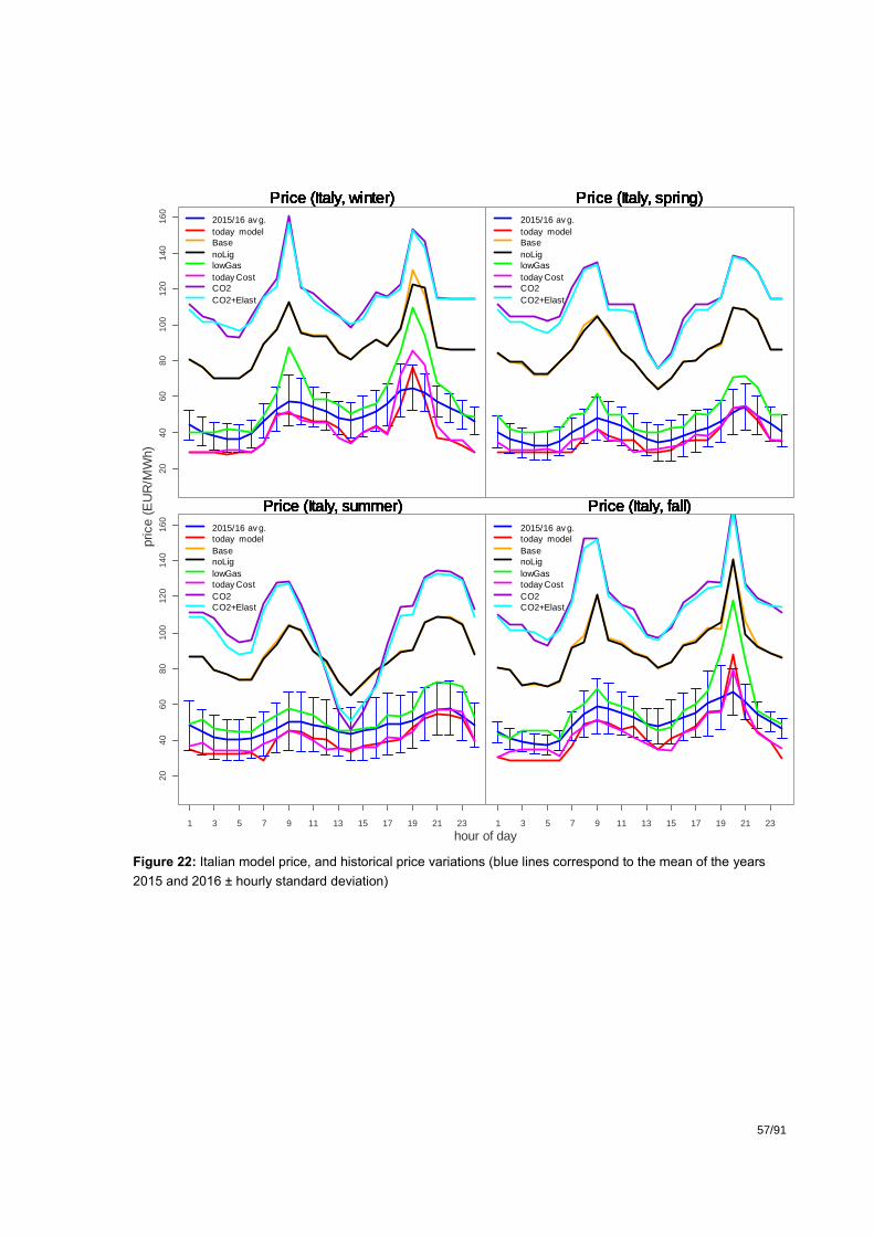
57/91
Figure 22: Italian model price, and historical price variations (blue lines correspond to the mean of the years
2015 and 2016 ± hourly standard deviation)
hour of day
price
(E
UR
/MW
h)
Price (Italy, winter)Price (Italy, winter)Price (Italy, winter)Price (Italy, winter)Price (Italy, winter)Price (Italy, winter)Price (Italy, winter)
2015/16 av g.
today model
Base
noLig
lowGas
today Cost
CO2
CO2+Elast
20
40
60
80
100
120
140
160
hour of day
price
(E
UR
/MW
h)
Price (Italy, spring)Price (Italy, spring)Price (Italy, spring)Price (Italy, spring)Price (Italy, spring)Price (Italy, spring)Price (Italy, spring)
2015/16 av g.
today model
Base
noLig
lowGas
today Cost
CO2
CO2+Elast
hour of day
price
(E
UR
/MW
h)
Price (Italy, summer)Price (Italy, summer)Price (Italy, summer)Price (Italy, summer)Price (Italy, summer)Price (Italy, summer)Price (Italy, summer)
2015/16 av g.
today model
Base
noLig
lowGas
today Cost
CO2
CO2+Elast
1 3 5 7 9 11 13 15 17 19 21 23
20
40
60
80
100
120
140
160
hour of day
price
(E
UR
/MW
h)
Price (Italy, fall)Price (Italy, fall)Price (Italy, fall)Price (Italy, fall)Price (Italy, fall)Price (Italy, fall)Price (Italy, fall)
2015/16 av g.
today model
Base
noLig
lowGas
today Cost
CO2
CO2+Elast
1 3 5 7 9 11 13 15 17 19 21 23
hour of day
price (
EU
R/M
Wh)

Oligopolistic capacity expansion with subsequent market-bidding under transmission constraints (OCESM)
58/91
Figure 23: Austrian model price, and historical price variations (blue lines correspond to the mean of the years
2015 and 2016 ± hourly standard deviation)
hour of day
price
(E
UR
/MW
h)
Price (Austria, winter)Price (Austria, winter)Price (Austria, winter)Price (Austria, winter)Price (Austria, winter)Price (Austria, winter)Price (Austria, winter)
2015/16 av g.
today model
Base
noLig
lowGas
today Cost
CO2
CO2+Elast
020
40
60
80
100
120
140
hour of day
price
(E
UR
/MW
h)
Price (Austria, spring)Price (Austria, spring)Price (Austria, spring)Price (Austria, spring)Price (Austria, spring)Price (Austria, spring)Price (Austria, spring)
2015/16 av g.
today model
Base
noLig
lowGas
today Cost
CO2
CO2+Elast
hour of day
price
(E
UR
/MW
h)
Price (Austria, summer)Price (Austria, summer)Price (Austria, summer)Price (Austria, summer)Price (Austria, summer)Price (Austria, summer)Price (Austria, summer)
2015/16 av g.
today model
Base
noLig
lowGas
today Cost
CO2
CO2+Elast
1 3 5 7 9 11 13 15 17 19 21 23
20
40
60
80
100
120
140
hour of day
price
(E
UR
/MW
h)
Price (Austria, fall)Price (Austria, fall)Price (Austria, fall)Price (Austria, fall)Price (Austria, fall)Price (Austria, fall)Price (Austria, fall)
2015/16 av g.
today model
Base
noLig
lowGas
today Cost
CO2
CO2+Elast
1 3 5 7 9 11 13 15 17 19 21 23
hour of day
price (
EU
R/M
Wh)

59/91
Table 20: Averaged hourly electricity prices over seasonal days and hourly volatilities (EUR). Vol = sd(log(price))
Winter Spring Summer Fall Annual
Mean Volatility Mean Volatility Mean Volatility Mean Volatility Mean Volatility
AT
today 32.9 15% 26.8 12% 27.8 14% 33.7 17% 30.3 15%
Base 93.7 9% 78.9 7% 78.2 8% 85.2 8% 84.0 8%
noLig 95.1 9% 78.9 8% 80.1 8% 87.6 8% 85.4 8%
lowGas 66.2 13% 48.2 9% 47.1 8% 59.1 13% 55.2 11%
todayCost 51.7 16% 37.2 9% 35.9 8% 44.8 12% 42.4 11%
CO2 110.1 7% 96.7 7% 82.8 11% 109.9 9% 99.9 9%
CO2+Elast 103.2 9% 90.5 8% 80.4 9% 108.0 9% 95.5 9%
DE
today 32.4 16% 27.6 9% 30.9 9% 34.8 14% 31.4 12%
Base 74.5 13% 68.8 16% 69.6 15% 83.1 17% 74.0 15%
noLig 86.8 16% 77.7 16% 78.5 14% 103.8 20% 86.7 16%
lowGas 60.3 15% 53.9 18% 56.0 16% 66.5 16% 59.2 16%
todayCost 41.2 19% 35.1 20% 37.7 17% 45.5 21% 39.9 19%
CO2 116.2 13% 107.1 15% 108.0 14% 123.4 12% 113.7 14%
CO2+Elast 111.2 15% 104.8 16% 106.1 14% 121.8 12% 111.0 14%
FR
today 32.5 14% 27.7 5% 32.0 7% 34.9 13% 31.8 10%
Base 21.6 20% 17.6 15% 19.8 14% 23.3 21% 20.6 17%
noLig 21.3 20% 17.6 15% 19.6 13% 22.8 21% 20.4 17%
lowGas 22.1 19% 18.1 15% 22.1 11% 24.6 20% 21.7 16%
todayCost 22.6 22% 18.7 13% 23.3 9% 25.6 19% 22.5 16%
CO2 20.5 18% 17.5 15% 19.3 14% 22.2 23% 19.9 18%
CO2+Elast 19.5 15% 17.4 14% 18.1 12% 20.7 22% 18.9 16%
IT
today 40.6 19% 35.7 12% 40.2 12% 43.0 19% 39.9 16%
Base 89.6 12% 85.4 10% 87.7 9% 91.4 13% 88.5 11%
noLig 89.4 11% 85.5 9% 87.6 9% 90.9 14% 88.3 11%
lowGas 59.8 17% 49.6 12% 53.7 10% 58.3 18% 55.3 14%
todayCost 42.7 23% 36.6 13% 41.2 11% 43.5 16% 41.0 16%
CO2 116.1 12% 111.4 11% 103.3 16% 117.8 13% 112.2 13%
CO2+Elast 115.0 12% 109.0 11% 101.0 15% 116.3 13% 110.3 13%
CH today 34.6 15% 29.4 8% 32.7 9% 36.6 14% 33.3 12%
Base 77.4 6% 64.0 8% 63.8 9% 71.0 12% 69.1 9%

Oligopolistic capacity expansion with subsequent market-bidding under transmission constraints (OCESM)
60/91
noLig 81.8 7% 66.1 9% 66.5 9% 77.2 13% 72.9 9%
lowGas 77.3 6% 44.8 10% 45.2 9% 53.8 14% 55.3 9%
todayCost 43.7 12% 33.2 11% 34.8 10% 41.5 15% 38.3 12%
CO2 92.1 9% 83.7 10% 77.6 11% 93.5 11% 86.7 10%
CO2+Elast 92.0 8% 82.4 9% 75.8 10% 92.0 10% 85.6 9%
Table 21: Historical hourly mean prices (EUR) and daily volatilities for the year 2015 and 2016. Vol = sd(log(price)
change)
Winter Spring Summer Fall Annual
Mean Volatility Mean Volatility Mean Volatility Mean Volatility Mean Volatility
AT 2015/16 30.3 45% 26.2 31% 29.8 15% 35.0 25% 30.3 29%
DE 2015/16 30.3 45% 26.2 31% 29.8 15% 35.0 25% 30.3 29%
FR 2015/16 40.8 15% 31.1 16% 31.7 12% 47.0 14% 37.6 14%
IT 2015/16 50.3 10% 41.2 12% 47.7 8% 51.1 10% 47.6 10%
CH 2015/16 47.7 9% 31.0 17% 30.8 12% 47.2 10% 39.1 12%
5.2.2. Endogenous Production and Investment
5.2.2.1. Switzerland
The phase-out of the existing nuclear capacity is completed in 2034/2035 and leads to a gap in the
electricity supply which is filled with increased penetration of non-hydro renewable technologies and
imports. In all market environments emerged from the assessed scenarios, no large-scale gas turbine
combined cycle plants are built in Switzerland by 2035.
Hydropower is the main contributor to the electricity supply in Switzerland (including net imports) with a
share from 50% (in the “LowGas” scenario) to 57% (in the “CO2” scenario) in 2035, from about 56% in
the “today” scenario. In absolute terms, the contribution of hydropower to the domestic electricity supply
increases in 2035 by at most 1 TWh/yr. from today’s level.
Biomass and solar PV account for about 7% each in the domestic generation on average across all
scenarios. Biomass has a total contribution of about 3.7 – 4.5 TWh/yr. in 2035, with the highest pene-
tration (4.5 TWh/yr.) occurring under stringent climate change mitigation policy (i.e. in the “CO2” and
“CO2 + Elast” scenarios). The electricity generation from solar PV amounts to 4.4 TWh/yr. in all scenar-
ios. On the other hand, the expansion of the wind turbines is limited in all scenarios, about 2 TWh/yr. by
2035, except in the “CO2” scenario where it increases to 4 TWh/yr. In the “CO2” scenario, the electricity
generation from wind is very close to its assumed potential.
Net imports of electricity amount from 12.5 TWh to 26.7 TWh, depending on the scenario. The lowest
amount of electricity imports (12.5 TWh) is in the “CO2” scenario, driven by the increased electricity
generation costs and the reduction of domestic demand compared to the “Base” scenario. On the other

61/91
hand, the highest amount of electricity imports (23.5 – 26.77 TWh) occurs when the gas prices are low
(“todayCost” and “lowGas” scenarios), driven by increased cross-border flows from Italy and Austria.
The investments in new generation capacity are mainly solar PV and to a lesser extent wind turbines.
In all scenarios, irrespectively of the intensity of the underlying climate change mitigation policy, about
6.4 GW of roof-top solar PV is additionally installed in Switzerland by 2035, which increase the cumula-
tive installed capacity of solar PV to close to 8 GW. About 1 GW of wind turbines is installed in all sce-
narios except the “CO2” scenario by 2035. In the “CO2” scenario the investments in wind turbines are
doubled and reach 2.6 GW in 2035. The investments in hydropower are limited and amount only to
about 250 MW in all scenarios, except the “LowGas” and “TodayCost” scenarios. Interestingly, when the
gas prices are low, then there is no investment in new hydropower units. This suggests that the expan-
sion of run-of-river hydropower is not profitable when low-cost imported electricity is available. On the
other hand, investments in biomass occur only under stringent climate change mitigation policy (i.e. in
the “CO2” and “CO2 + Elast” scenarios), but they are somewhat small (about 120 MW).
Finally, the electricity load increases from 58 TWh in the “Today” scenario to 63 TWh in the “Base”
scenario and around 59 TWh in the “CO2” and “CO2 + Elast” scenarios. In the case of low gas prices,
the electricity load in Switzerland increases to 66 TWh in the “LowGas” scenario and 70 TWh in the
“TodayCost” scenarios. In the “NoLignite” scenario the electricity load in Switzerland is slightly lower
than the “Base” scenario to 62 TWh.
5.2.2.2. Neighbouring countries
In Germany, the nuclear phase-out, which is completed before 2035, turns the country from a net ex-
porter of electricity to a net importer in all scenarios of the market model (Figure 25). In the “Base”
scenario, the gap in electricity supply arising from decommissioning of the existing nuclear capacity and
increased demand is mainly filled by additional generation from wind turbines, biomass, solar PV and
imported electricity, while solid-based generation (lignite and coal) retains a high share in the domestic
supply as in the “Today” scenario. On the other hand, under stringent climate policy (“CO2” and “CO2 +
Elast” scenarios), the electricity generation from lignite and coal is replaced by increased production
from gas turbine combined-cycle plants and solar PV compared to the “Base” scenario. Similarly, in the
“LowGas” scenario the electricity generation from gas gains share in the domestic supply mix, mainly at
the expense of coal-based generation. On the other hand, the electricity generation from lignite in the
“LowGas” scenario remains unchanged compared to the “Base” scenario, since lignite power plants
remain competitive as long as there is no stringent climate-change mitigation policy in place. However,
in the “NoLignite” scenario, the decommissioning of the low-cost lignite generation increases the
electricity production costs, which in turn result in lower electricity load. In this context, the lignite gen-
eration of the “Base” scenario is substituted by about 31% from coal and 42% from gas, while the rest
27% is attributable to the reduction of the load that occurs in this scenario as a response to the increased
electricity prices.
Regarding the investments in new generation capacity in Germany, there is a significant increase in the
installed capacity of wind turbines and solar PV in all scenarios compared to the “Today” scenario (Figure
30). The expansion of wind turbines and solar PV is more pronounced under stringent climate policy,
while low gas prices hinder investments in intermittent generation. In this context, the investment in wind
turbines amounts to 24GW in the “LowGas” and “TodayCost” scenarios and increase to 42 GW in the
rest of the assessed scenarios. This implies that the assumed potential of 87 GW of wind onshore tur-
bines in Germany is fully met in all scenarios except those with low gas prices. The investments in solar
PV amount to 31 GW in all the non-CO2 scenarios by 2035. They reach 53 GW in the “CO2” scenario
by 2035. However, in the “CO2 + Elast” scenario, the investments in solar PV are only slightly higher
than the investments in the non-CO2 scenarios: around 35 GW by 2035. This outcome is mainly driven
Oligopolistic capacity expansion with subsequent market-bidding under transmission constraints (OCESM)
62/91
by the significantly lower load attained in this scenario. Investments in gas turbine combined cycle plants
occur in the “TodayCost” scenario (2 GW) in the “LowGas” scenario (11 GW) and the “CO2” scenario
(5 GW). In all other scenarios, there are no investments in gas-based electricity generation. This result
suggests that the investments in gas power plants are driven by the gas and CO2 prices. In the “CO2”
scenario, the high CO2 prices hamper the profitability of lignite and coal power plants enabling invest-
ments in gas-based power capacity. On the other hand, in the “TodayCost” scenario, the low CO2 prices
maintain the profitability of the coal-based power plants resulting in low electricity prices; in this context,
the low gas prices in this scenario are not sufficient to significantly drive investments in gas turbine
combined cycle plants. However, in the “LowGas” scenario, the high CO2 prices hamper the profitability
of the coal-based power plants, and this results in high electricity prices; in this case, the low gas prices
in this scenario boost investments in gas turbine combined cycle plants. On the other hand, investments
in biomass remain the same across all scenarios, since biomass reaches its assumed potential of 2035
in any case.
In France, nuclear power maintains its dominant share in the domestic electricity generation mix despite
the decommissioning of about 6.3 GW by 2035 (Figure 26). The gap in electricity supply due to the
increased electricity load and the retirement of the nuclear power capacity is met by additional genera-
tion from wind turbines and solar PV. Since fossil-based generation does not occur in France in any
scenario, the electricity sector remains carbon-free and mostly unaffected by the levels of the CO2 and
gas prices. In this context, the generation mix of France, as well as the level of the electricity load, is the
same across all scenarios. It follows that investments in new generation capacity are towards biomass,
wind, and solar PV (Figure 31); about 30 GW of wind turbines and 31 GW of solar PV are installed in
France by 2035, while investments in biomass amount to 2 GW.
In Italy, the implementation of the renewable electricity generation targets reduces the share of fossil-
based generation in the “Base” scenario compared with the “Today” scenario (Figure 27). Biomass, wind
turbines and solar PV mainly substitute gas-based generation in this scenario, and they also supply the
increased demand. Gas is competitive only when low gas prices prevail in the Italian market, and in this
case, coal generation is phased out. The amount of net imports in Italy significantly reduces in all sce-
narios compared to the “Today” scenario, mainly due to the shift of Switzerland from a net exporter to a
net importer by 2035. With the exception of the low gas price scenarios, the electricity load in Italy slightly
increases in all scenarios by 2035 from “Today” levels as the electricity prices in Italy remain at high
levels. As in Germany and France, the investments in the Italian electricity sector are towards wind
turbines, solar PV and biomass (Figure 32). Such investments in renewable energy are highest under
stringent climate policy and lowest in the scenarios with low gas prices. However, there are no invest-
ments in additional gas-based power plants, even in the “LowGas” and “TodayCost” scenarios where
the electricity generation costs from gas are the lowest across all scenarios. This implies that the in-
creased contribution of gas power plants in the electricity supply mix in these scenarios is the outcome
of higher utilisation rates and not of capacity expansion.
Finally, in Austria, biomass, wind and solar PV increase their share in the electricity generation mix in
all scenarios compared to the “Today” scenario (Figure 28). Hydropower does not expand in Austria as
most of its potential has been already exploited. However, in order to supply the increased demand and
the increased exports to Switzerland, additional generation from fossil fuels is foreseen in all scenarios.
As in the case of Germany and Italy, the penetration of gas-based generation is highest under low gas
prices. Under a stringent climate policy, the domestic electricity load in Austria reduces significantly,
while the fossil-based generation is almost phased-out; in this case, solar PV increases its contribution

63/91
to the domestic supply. Similarly to the rest of the countries, the investments in Austria are mostly ori-
ented towards non-hydro renewable energy (Figure 33). On the other hand, there are no capacity
additions to fossil-based generation (with the exception of 2 GW investments in gas turbine combined
cycle plants in the “LowGas” scenario for reasons similar to the ones observed in Germany), which
implies that the increased generation from coal and gas observed in all scenarios is mainly the outcome
of a higher utilisation of the existing capacity.
7
Figure 24: Swiss production and system load in the
market model. Today’s production mix is also endoge-
nously calculated by the market model
Figure 25: German production and system load in the
market model. Today’s production mix is also endoge-
nous calculated by the market model
-10
0
10
20
30
40
50
60
70
TW
h
Switzerland Net Imports
Pump
SolarPV
WindOnshore
HydroStorage
HydroRoR
Biomass
Nuclear
GasCC
GasTurbine
GasSteam
OilCC
OilTurbine
OilSteam
Coal
Lignite
Load
-100
0
100
200
300
400
500
600
700
TW
h
Germany
Net Imports
Pump
SolarPV
WindOnshore
HydroStorage
HydroRoR
Biomass
Nuclear
GasCC
GasTurbine
GasSteam
OilCC
OilTurbine
OilSteam
Coal
Lignite
Load

Oligopolistic capacity expansion with subsequent market-bidding under transmission constraints (OCESM)
64/91
Figure 26: French production and system load in the
market model. Today’s production mix is also endoge-
nous calculated by the market model
Figure 27: Italian production and system load in the
market model. Today’s production mix is also endoge-
nous calculated by the market model
Figure 28: Austrian production and system load in the
market model. Today’s production mix is also endoge-
nously calculated by the market model
-100
0
100
200
300
400
500
600
TW
h
France Net Imports
Pump
SolarPV
WindOnshore
HydroStorage
HydroRoR
Biomass
Nuclear
GasCC
GasTurbine
GasSteam
OilCC
OilTurbine
OilSteam
Coal
Lignite
Load
0
50
100
150
200
250
300
350
400
TW
h
Italy Net Imports
Pump
SolarPV
WindOnshore
HydroStorage
HydroRoR
Biomass
Nuclear
GasCC
GasTurbine
GasSteam
OilCC
OilTurbine
OilSteam
Coal
Lignite
Load
-40
-20
0
20
40
60
80
100
TW
h
Austria Net Imports
Pump
SolarPV
WindOnshore
HydroStorage
HydroRoR
Biomass
Nuclear
GasCC
GasTurbine
GasSteam
OilCC
OilTurbine
OilSteam
Coal
Lignite
Load

65/91
Figure 29: Swiss region investments in the market
model
Figure 30: German region investments in the market
model
Figure 31: French region investments in the market
model
Figure 32: Italian region investments in the market
model
0123456789
10
GW
Investment, Switzerland
SolarPV
WindOnshore
HydroRoR
Biomass
Nuclear
GasCC
0
20
40
60
80
100
120
GW
Investment, Germany
SolarPV
WindOnshore
HydroRoR
Biomass
Nuclear
GasCC
0
10
20
30
40
50
60
70
GW
Investment, France
SolarPV
WindOnshore
HydroRoR
Biomass
Nuclear
GasCC
0
10
20
30
40
50
60
70
80
GW
Investment, Italy
SolarPV
WindOnshore
HydroRoR
Biomass
Nuclear
GasCC

Oligopolistic capacity expansion with subsequent market-bidding under transmission constraints (OCESM)
66/91
Figure 33: Austrian region investments in the market
model
5.2.3. Cross-border electricity flows
Figure 34 displays the electricity flows across the five countries in the “Base” and the “CO2” scenario.
Compared with the “Today” scenario, the nuclear phase-out in Germany and Switzerland (in combination
with the increased electricity demand) turns these countries to net importers of electricity. Also, by 2035
not only France but also Austria becomes a net exporter of electricity supplying mainly the German and
Swiss markets. In this market situation, the Italian market is also affected because a large part of the
low-cost French electricity is directed to Switzerland and Germany by 2035.
5.2.3.1. Switzerland
On average, and across all scenarios, the Swiss net imports of electricity are close to the amount of
electricity produced by the existing nuclear power plants, i.e. close to 20 TWh/yr, especially when there
is no stringent climate change mitigation policy in place. In the case of the “CO2” and “CO2 + Elast”
scenario the net imports in Switzerland are about one fourth less than the imports in the “Base” scenario,
which is attributable to the higher cross-border electricity prices, to the increased deployment of renew-
ables and the reduction of electricity load.
Figure 35 presents the total cross-border flows on the typical hours of the model between Switzerland
and its neighbours. In all scenarios, except “Today”, Switzerland constantly imports electricity during the
winter and autumn. In spring and summer, net imports mainly occur during the off-peak hours, while
during the peak hours Switzerland exports electricity to Germany from hydropower plants. Notably, the
electricity exports during the peak hours in spring and summer in all scenarios are much higher than the
exports in the “Today” scenario. This result indicates that in seasons with good water resource availa-
bility, there are opportunities for arbitrage for the Swiss hydrostorage plants. The highest exports occur
under stringent climate change mitigation policy, which renders non-cost effective the fossil-based elec-
tricity generation in Germany. As already discussed in section 5.2.1.1, the Swiss electricity price is af-
fected by the increased exports to Germany, and during the peak hours in spring and summer remains
at very high levels, since the Swiss hydroelectricity producers sell their production close to the prices
attained in Germany.
02468
101214161820
GW
Investment, Austria
SolarPV
WindOnshore
HydroRoR
Biomass
Nuclear
GasCC

67/91
5.2.3.2. Neighboring countries
Germany is a net exporter of electricity in the “Today” scenario, exporting almost 90% of the time; it
imports electricity mainly during the summer peak hours from France. However, as stated in previous
sections, Germany turns into a net importer of electricity in all scenarios. In Germany the shift from a
net exporter to a net importer is almost on a one-to-one basis: the same amount of electricity which is
exported from Germany in the “Today” scenario is approximately also imported in all scenarios by 2035.
France remains a net exporter of electricity in all scenarios. In fact, its exports increase from the levels
of the “Today” scenario, mainly towards Germany and to a lesser extent towards Switzerland and Italy.
Italy remains a net importer of electricity in all scenarios, consistent with the trends observed in the
“Today” scenario. However, the nuclear phase out in Germany and Switzerland and, consequently, the
transformation of these two countries into net importers of energy, significantly impact the level of the
electricity imports in Italy. In this context, the Italian imports are reduced by almost 14 TWh in the “Base”
scenario compared to the “Today” scenario. Similar levels of reduction in the Italian imports are also
observed in the rest of the scenarios. Notably, Italy becomes almost self-sufficient in the scenarios with
low gas prices, attributable to the additional investments in gas power. Under stringent climate change
policy (“CO2” and “CO2 + Elast” scenarios) the net imports in Italy decline by about 10 TWh, driven by
the higher deployment of renewable electricity and the reduction in Italian electricity load. It is also worthy
to mention that the magnitude of the reduction in the Italian imports is almost equal to the increase of
the Swiss imports in all scenarios.
Finally, Austria turns from a net importer of electricity in the “Today” scenario into net exporter in all the
rest of scenarios by 2035. In this sense, it does not only supply the Italian market as it is the case in the
“Today” scenario, but also the markets of Germany and Switzerland. The shift of Austria from a net
importer to net exporter occurs almost on a one-to-one basis, in terms of energy: from 13.6 TWh net
imports in “Today”, Austria exports 12.6 – 16.6 TWh in the rest of the scenarios. Higher exports occur
under stringent climate change policy, due to the contribution of hydropower and renewables.

Oligopolistic capacity expansion with subsequent market-bidding under transmission constraints (OCESM)
68/91
Figure 34: Average power flows (MW) in the Base and CO2 high price scenario
Figure 35: Cross-border trade between Switzerland and neighbouring countries in the typical hours (positive
values denote imports, negative values denote exports)
-5000
-4000
-3000
-2000
-1000
0
1000
2000
3000
4000
5000
WI-
D-0
1
WI-
D-0
4
WI-
D-0
7
WI-
D-1
0
WI-
D-1
3
WI-
D-1
6
WI-
D-1
9
WI-
D-2
2
SP
-D-0
1
SP
-D-0
4
SP
-D-0
7
SP
-D-1
0
SP
-D-1
3
SP
-D-1
6
SP
-D-1
9
SP
-D-2
2
SU
-D-0
1
SU
-D-0
4
SU
-D-0
7
SU
-D-1
0
SU
-D-1
3
SU
-D-1
6
SU
-D-1
9
SU
-D-2
2
FA
-D-0
1
FA
-D-0
4
FA
-D-0
7
FA
-D-1
0
FA
-D-1
3
FA
-D-1
6
FA
-D-1
9
FA
-D-2
2
MW
Switzerland
Today
Base
LowGas
NoLignite
TodayCost
CO2
CO2+Elast

69/91
5.2.4. Profit of power production
In Switzerland, the operational profit of power producers (aggregated to whole countries) increases in
all scenarios compared with the parametrization of “Today”, which approximates the current market re-
sults in the model. The operational profit in the model by our definition for this report is the following
sum:
+ Price * Quantity (over the load periods)
– Price * Quantity used for pumping (hydropower)
– Costs for ramping, start-up etc. (thermal production)
– Fuel costs
– Variable O&M costs.
A major driver of the operational profit is the higher electricity price because of higher fossil fuel prices
(Figure 36). However, in the “LowGas” scenario, the profitability of the Swiss suppliers remains at the
same levels of the “Today” scenario, because of the reduced electricity prices in “LowGas”. On the other
hand, the highest increase in profitability occurs under a stringent climate policy, driven by the signifi-
cantly higher electricity prices that outweigh the increased generation costs in such a scenario and the
retaining of the demand at levels of “Today”.
Similarly to Switzerland, the profitability of the electricity sector in the rest of the countries also increases
in all scenarios compared to “Today”, except in France. The lowest profitability occurs when the gas
prices are low, and the highest profitability is under a stringent climate change mitigation policy. Across
all countries, the largest increase in profitability occurs in Austria and to a lesser extent in Italy, which
are the countries with the highest increase in electricity prices due to additional contribution from fossil-
based generation compared with “Today”. On the other hand, in France, the profitability of the suppliers
reduces in all scenarios compared with the “Today” scenario, driven by the significantly lower electricity
prices (see Section 5.2.1.2).

Oligopolistic capacity expansion with subsequent market-bidding under transmission constraints (OCESM)
70/91
Figure 36: Change of operational profit of power production in the differ-
ent scenarios relative to “today” (in aggregate for the production portfolio
of the countries)
In particular, we show next the net profit of gas-combined cycle (gas-CC) and hydropower technolo-
gies over the scenarios. Please note that the definition of net profit is ambiguous, and the definition
and rough calculation in this report may not be adequate for other purposes. The net profit as as-
sumed in our report is the following sum:
+ Price * Quantity (over the load periods)
– Price * Quantity used for pumping (hydropower)
– Costs for ramping, start-up etc. (thermal production)
– Fuel costs
– Variable O&M costs
– Fixed O&M costs
– Capital costs (5% discount rate).
For gas-CC plants, we make the following assumptions: The lifetime of the plant is 30 years; the plant
is newly built; the price-results of each scenario in year 2035 prevail during the lifetime. The resulting
net profit is shown in Figure 37. As of today, build new gas plants seems not to be profitable, and this
will not change under the Base scenario (which has a changed capacity mix with less fossil and more
renewable generation, and higher fuel costs). Gas-CC plants become profitable under the “LowGas”
and the “TodayCost” scenario, mainly in Germany and Austria, where the gas plants can run in base
load to replace the vanishing nuclear and coal base-load production. In Germany, it seems that they can
be profitable even in the high CO2-price scenarios. In Italy, the net profit for newly built plants is near
zero, which results in now gas-CC plants built in all scenarios. Hence, it seems that gas plants cannot
operate at enough load hours to produce enough operational profit.

71/91
Figure 37: Net profitability (operational profit – costs; see text) of new gas gas-combined cy-
cle plants per unit capacity
Next, we consider the hydropower plants in Switzerland. We make the following rough assumptions. We
assume a lifetime of 60 years, which results in an average (weighted by production) lifetime of the cur-
rent stock of hydropower of 28 years. Hence, we may assume that half of the capital costs are written
off, such that we reduce (by rough assumption) the capital cost by a half; for the capital stock, we assume
40 bio. CHF (SWV, 2012 / 2016 revised), and we assume for the water tax the year 2015 value
(557 mio. CHF). According to the BFE report of (Fillipini, 2014), about half of the cost of hydropower
production can be attributed to capital cost and water taxes; we assume 75%. For the scenarios in the
future, we assume that these costs share (capital + watertax + other cost) stays approximately the same.
In fact, it is difficult to foresee when hydropower plants have to refurbished. Hence we assume in the
future scenarios the same amortization structure, and that the operational profit is according to the sce-
nario and prevails. Under these assumptions, we obtain the net profit per unit of energy produced in
Figure 38. As of today, hydropower seems to be barely profitable, and if fossil fuel costs stay as low as
of today (“todayCost” scenario), this may not change. In fact, Switzerland as a small country can be
considered as a price-taker on the day-ahead power market (see Section 5.2.1.1), such that the higher
future fossil fuel prices (especially gas) drives the future prices in Switzerland. Hence, in such scenarios,
the profit of Swiss hydropower can rise again, irrespective of the policy-driven, large deployment of new
renewables in these scenarios.

Oligopolistic capacity expansion with subsequent market-bidding under transmission constraints (OCESM)
72/91
Figure 38: Net profit (operational profit – costs; see text) of Swiss hydropower per
unit of power produced.

73/91
6. Auxiliary Results
6.1. Marginal (high-cost) technology
On an electricity market, the marginal technology is the technology that is associated with the highest
production-bid that has the highest value, and that is selected for production by the market-clearing
algorithm. In fact, the bid that is issued by a trader may not be associated to a technology and its specific
variable O&M and fuel cost at all, such that in a market environment the concept of marginal technology
is ambiguous. An alternative definition of a marginal technology would be the specific technology that is
not producing fully at its capacity bound; whereas the other technologies that are producing have their
production bounded by some constraint (availability etc.), for example, in most cases they are producing
fully at their capacity bound (sub-marginal technologies). The problem with this definition is that for
example in a Nash-Cournot setting; there may be several technologies not fully producing, even without
transmission constraints (e.g. see Table 3.2, p. 99 in Gabriel et al., 2013).
Despite the limited explanatory power and questionable concept, we may still determine in each load
period the specific domestic technology in a market area that is not producing at its capacity bound and
not hitting other availability constraints and has highest operational costs (variable O&M + fuel cost).
We call this technology in the following the (domestic) high-cost technology. The results are shown in
Table 22, Table 23 and Figure 39 - Figure 43.
In Switzerland, the high-cost technology in the “today” scenario is in 75% of the hours the nuclear power
plants (Figure 39). After the nuclear phase-out biomass generation (which incl. waste in our modelling)
is 75–80% of all load periods the high-cost technology, particularly in winter, spring, and fall. Intermittent
renewables and hydro become the high-cost (in fact almost “zero-cost”) domestic technology mainly
during the summer when the demand is low and can be met by these sources (and imports) without
dispatching thermal units. Note that the market model does not include cogeneration which could imply
must-run conditions in some end-use sectors.
In Germany, the high-cost technology in the “today” scenario is coal and gas combined-cycle plants,
with a share of 50% each. This implies that lignite and nuclear power plants are dispatched in the base-
load, while coal and gas are brought online to supply medium and peak load. However, after the nuclear-
phase out in the “Base” scenario, coal emerges more often than gas as the marginal domestic technol-
ogy, driven by the higher CO2 prices compared to the “Today” scenario. In the “NoLingite” scenario, the
phase-out of lignite-fuelled power plants result in increased generation from coal to meet the baseload
demand, while gas-based technologies are the most often domestic high-cost technology. In the “Low-
Gas”(-price) scenario, the favourable conditions for gas generation allow gas combined-cycle plants to
produce baseload and medium load electricity. Hence, in this scenario, coal generation is more expen-
sive than gas, and coal power becomes the high-cost technology in about 50% of the load periods; the
other 50% of the load periods are gas-based units for peak load. Under a stringent climate policy, the
high CO2 prices increase lignite and coal production costs, and gas combined-cycle plants have approx-
imately the same or even lower operational costs than coal and lignite plants and are dispatched more.
As in the case of Switzerland, renewable technologies are the “high-cost” technology during summer
where solar has high availability.
In France, the nuclear power covers baseload and most of the medium load in all scenarios (Figure 41).
The high-cost technology in France is biomass, reflecting the simple domestic electricity production mix
of the country.

Oligopolistic capacity expansion with subsequent market-bidding under transmission constraints (OCESM)
74/91
In Italy, the main marginal technology is gas turbine combined-cycle, which is dispatched during medium
and peak load in all scenarios (). Coal-based electricity generation is mostly dispatched for baseload,
except in the “LowGas” scenario. In this scenario, the low gas prices allow gas generation also for
baseload, with the result that coal power is the high-cost technology mainly during the peak hours of fall
and winter by ramping over 3-4 hours. Similar to Switzerland and Germany, under a stringent climate
policy, renewables become the high-cost technology during summer.
In Austria, the high-cost technology is mainly the gas combined-cycle plant, which is dispatched during
medium and peak load. Similar to the other countries, under a stringent climate policy renewables
emerge as the high-cost technology in summer. Biomass, which is the high-cost technology in 50% of
the load periods in the “Today” scenario, is also the high-cost technology under a stringent climate policy
mainly during spring.
Table 22: Domestic high-cost technology: Technology with highest variable cost (incl. fuel cost and CO2 cost) and
not hitting production bounds, for scenario “Base”, “NoLignite”, “LowGas”, and “TodayCost”. Abbreviations: B =
Biomass/Waste, C = Coal, GCC = Gas Combined Cycle, Gst = Gas Steam Turbine, L= Lignite, N = Nuclear,
OilCC = Oil Combined Cycle, R = Renewables (having zero short-term variable costs)
Scen -> Base noLignite lowGas todayCost
Period DE AT IT FR CH DE AT IT FR CH DE AT IT FR CH DE AT IT FR CH
Win
ter
1 R GCC GCC N - C GCC GCC B B GSt GSt GCC B B GSt GSt GCC B B
2 - GCC GCC N - C GCC GCC B B GSt GSt GCC B B GSt GSt GCC B B
3 - GCC GCC N - C GCC GCC B B GSt GSt GCC B B GSt GSt GCC B B
4 - GCC GCC N - C GCC GCC B B GSt GSt GCC B B GSt GSt GCC B B
5 - GCC GCC N - C GCC GCC B B GSt GSt GCC B B GSt GSt GCC B B
6 R GCC GCC N - C GCC GCC B B GSt GSt GCC B B GSt GSt GCC B B
7 C GCC GCC N - C GCC GCC B B GSt GSt GCC B B GSt GSt GCC B B
8 C - GCC N - GCC GCC GCC B B GSt GSt GCC B B GSt GSt GCC B B
9 R - - N - GCC GCC GCC B B GSt C GCC B B GSt GSt GCC B B
10 - - - N - GCC GCC GCC B B GSt C GCC B B GSt GSt GCC B B
11 - - GCC N - GCC GCC GCC B B GSt C GCC B B GSt GSt GCC B B
12 C - GCC N - GCC GCC GCC B B GSt C GCC B B GSt GSt GCC B B
13 C - GCC N - GCC GCC GCC B B GSt C GCC B B GSt GSt GCC B B
14 C - GCC N - GCC GCC GCC B B GSt C GCC B B GSt GSt GCC B B
15 - - GCC N - GCC GCC GCC B B GSt C GCC B B GSt GSt GCC B B
16 - - GCC N - GCC GCC GCC B B GSt C GCC B B GSt GSt GCC B B
17 GCC - GCC N - OilCC GCC GCC B B C C GSt B B GSt GSt GCC B B
18 R - GCC N - OilCC GCC GCC B B C C C B B GSt GSt GSt B B
19 R - - - - OilCC GCC GCC B B C C C B B GSt GSt GSt B B
20 GCC - - - - OilCC GCC GCC B B C C C B B GSt GSt GSt B B
21 GCC - GCC N - GCC GCC GCC B B GSt C C B B GSt GSt GSt B B
22 C - GCC N - GCC GCC GCC B B GSt C GSt B B GSt GSt GCC B B
23 C - GCC N - C GCC GCC B B GSt C GCC B B GSt GSt GCC B B
24 C GCC GCC N - C GCC GCC B B GSt GSt GCC B B GSt GSt GCC B B
Sp
rin
g
1 C GCC GCC - R GCC GCC GCC B B L GCC GCC B B GCC GCC GCC B B
2 C GCC GCC N - GCC GCC GCC B B L GCC GCC B B GCC GCC GCC B B
3 C GCC GCC N - GCC GCC GCC B B L GCC GCC B B GCC GCC GCC B B
4 C GCC GCC N - GCC GCC GCC B B L GCC GCC B B GCC GCC GCC B B
5 C GCC GCC N - GCC GCC GCC B B L GCC GCC B B GCC GCC GCC B B
6 C GCC GCC N R GCC GCC GCC B B L GCC GCC B B GCC GCC GCC B B
7 R R GCC N R GCC GCC GCC B B L GCC GCC B B GCC GCC GCC B B
8 R R - - R GCC GCC GCC B B L GCC GCC B B GCC GCC GCC B B
9 R R - - R GCC GCC GCC B B L GCC GCC B B GCC GCC GCC B B

75/91
10 C R - N R GCC GCC GCC B B L GCC GCC B B GCC GCC GCC B B
11 C R GCC N R GCC GCC GCC B B L GCC GCC B B GCC GCC GCC B B
12 C - GCC N R GCC GCC GCC B B L GCC GCC B B GCC GCC GCC B B
13 C GCC GCC N R GCC GCC GCC B B L GCC GCC B B GCC GCC GCC B B
14 C GCC GCC N - GCC GCC GCC B B L GCC GCC B B GCC GCC GCC B B
15 C GCC GCC N - GCC GCC GCC B B L GCC GCC B B GCC GCC GCC B B
16 C GCC GCC N - GCC GCC GCC B B L GCC GCC B B GCC GCC GCC B B
17 C GCC GCC N R GCC GCC GCC B B L GCC GCC B B GCC GCC GCC B B
18 C R GCC N R GCC GCC GCC B B GSt GCC GCC B B GCC GCC GCC B B
19 GCC R - N R GCC GCC GCC B B GSt GCC GCC B B GCC GCC GCC B B
20 R R - N R GCC GCC GCC B B GSt GCC GCC B B GCC GCC GCC B B
21 R R - R R GCC GCC GCC B B GSt GCC GCC B B GCC GCC GCC B B
22 GCC R - - R GCC GCC GCC B B GSt GCC GCC B B GCC GCC GCC B B
23 R R GCC R R GCC GCC GCC B B GSt GCC GCC B B GCC GCC GCC B B
24 C GCC GCC R R GCC GCC GCC B B L GCC GCC B B GCC GCC GCC B B
Su
mm
er
1 C - GCC R - GCC C GCC B R L GCC GCC B R GCC GCC GCC B R
2 C - GCC N - GCC C GCC B R L GCC GCC B R GCC GCC GCC B R
3 C - GCC N - GCC C GCC B R L GCC GCC B R GCC GCC GCC B R
4 C - GCC N - GCC C GCC B R L GCC GCC B R GCC GCC GCC B R
5 C - GCC N - GCC C GCC B R L GCC GCC B R GCC GCC GCC B R
6 C - GCC N - GCC C GCC B R L GCC GCC B R GCC GCC GCC B R
7 R - GCC N - GCC C GCC B R L GCC GCC B R GCC GCC GCC B R
8 R R - N - GCC C GCC B R L GCC GCC B R GCC GCC GCC B R
9 R R - N - GCC C GCC B R L GCC GCC B R GCC GCC GCC B R
10 R R - N - GCC C GCC B R L GCC GCC B R GCC GCC GCC B R
11 C R GCC N - GCC C GCC B R L GCC GCC B R GCC GCC GCC B R
12 C R GCC N - GCC C GCC B R L GCC GCC B R GCC GCC GCC B R
13 C R GCC N - GCC C GCC B R L GCC GCC B R GCC GCC GCC B R
14 C - GCC N - GCC C GCC B R L GCC GCC B R GCC GCC GCC B R
15 C - GCC N - GCC C GCC B R L GCC GCC B R GCC GCC GCC B R
16 C - GCC N - GCC C GCC B R L GCC GCC B R GCC GCC GCC B R
17 C - GCC N - GCC C GCC B R L GCC GCC B R GCC GCC GCC B R
18 C R GCC N - GCC C GCC B R L GCC GCC B R GCC GCC GCC B R
19 R R GCC N - GCC C GCC B R GSt GCC GCC B R GCC GCC GCC B R
20 R R - N - GCC C GCC B R GSt GCC GCC B R GCC GCC GCC B R
21 R R - R - GCC C GCC B R GSt GCC GCC B R GCC GCC GCC B R
22 R R - R - GCC C GCC B R GSt GCC GCC B R GCC GCC GCC B R
23 R R - R - GCC C GCC B R GSt GCC GCC B R GCC GCC GCC B R
24 C - GCC R - GCC C GCC B R GSt GCC GCC B R GCC GCC GCC B R
Fa
ll
1 C GCC GCC N - GCC GCC GCC N B GSt GCC GCC B B GSt GSt GCC B B
2 C GCC GCC N - GCC GCC GCC N B GSt GCC GCC B B GSt GSt GCC B B
3 C GCC GCC N - GCC GCC GCC N B GSt GCC GCC B B GSt GSt GCC B B
4 C GCC GCC N - GCC GCC GCC N B GSt GCC GCC B B GSt GSt GCC B B
5 C GCC GCC N - GCC GCC GCC N B GSt GCC GCC B B GSt GSt GCC B B
6 C GCC GCC N - GCC GCC GCC N B GSt GCC GCC B B GSt GSt GCC B B
7 GCC GCC GCC N - GSt GCC GCC N B GSt GCC GCC B B GSt GSt GCC B B
8 R R - N - OilCC GCC GCC N B C GCC GCC B B GSt GSt GCC B B
9 R R - N - OilCC GCC GCC N B C GCC GCC B B GSt GSt GCC B B
10 R R GCC N - OilCC GCC GCC N B C GCC GCC B B GSt GSt GCC B B
11 GCC R GCC N - GSt GCC GCC N B GSt GCC GCC B B GSt GSt GCC B B
12 GCC R GCC N - GCC GCC GCC N B GSt GCC GCC B B GSt GSt GCC B B
13 GCC GCC GCC N - GCC GCC GCC N B GSt GCC GCC B B GSt GSt GCC B B
14 GCC GCC GCC N - GCC GCC GCC N B GSt GCC GCC B B GSt GSt GCC B B
15 GCC GCC GCC N - GCC GCC GCC N B GSt GCC GCC B B GSt GSt GCC B B
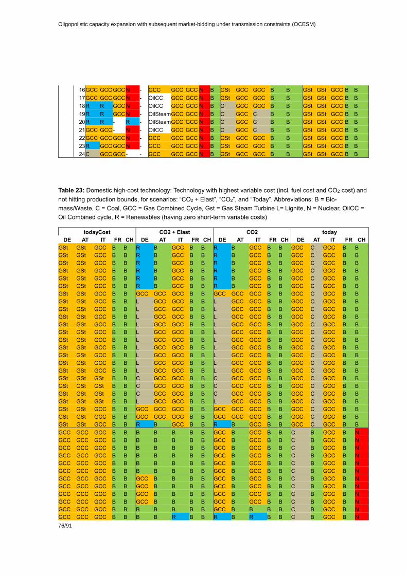
Oligopolistic capacity expansion with subsequent market-bidding under transmission constraints (OCESM)
76/91
16 GCC GCC GCC N - GCC GCC GCC N B GSt GCC GCC B B GSt GSt GCC B B
17 GCC GCC GCC N - OilCC GCC GCC N B GSt GCC GCC B B GSt GSt GCC B B
18 R R GCC N - OilCC GCC GCC N B C GCC GCC B B GSt GSt GCC B B
19 R R GCC N - OilSteam GCC GCC N B C GCC C B B GSt GSt GCC B B
20 R R - R - OilSteam GCC GCC N B C GCC C B B GSt GSt GCC B B
21 GCC GCC - N - OilCC GCC GCC N B C GCC C B B GSt GSt GCC B B
22 GCC GCC GCC N - GCC GCC GCC N B GSt GCC GCC B B GSt GSt GCC B B
23 R GCC GCC N - GCC GCC GCC N B GSt GCC GCC B B GSt GSt GCC B B
24 C GCC GCC - - GCC GCC GCC N B GSt GCC GCC B B GSt GSt GCC B B
Table 23: Domestic high-cost technology: Technology with highest variable cost (incl. fuel cost and CO2 cost) and
not hitting production bounds, for scenarios: “CO2 + Elast”, “CO2”, and “Today”. Abbreviations: B = Bio-
mass/Waste, C = Coal, GCC = Gas Combined Cycle, Gst = Gas Steam Turbine L= Lignite, N = Nuclear, OilCC =
Oil Combined cycle, R = Renewables (having zero short-term variable costs)
todayCost CO2 + Elast CO2 today
DE AT IT FR CH DE AT IT FR CH DE AT IT FR CH DE AT IT FR CH
GSt GSt GCC B B R B GCC B B R B GCC B B GCC C GCC B B
GSt GSt GCC B B R B GCC B B R B GCC B B GCC C GCC B B
GSt GSt GCC B B R B GCC B B R B GCC B B GCC C GCC B B
GSt GSt GCC B B R B GCC B B R B GCC B B GCC C GCC B B
GSt GSt GCC B B R B GCC B B R B GCC B B GCC C GCC B B
GSt GSt GCC B B R B GCC B B R B GCC B B GCC C GCC B B
GSt GSt GCC B B GCC GCC GCC B B GCC GCC GCC B B GCC C GCC B B
GSt GSt GCC B B L GCC GCC B B L GCC GCC B B GCC C GCC B B
GSt GSt GCC B B L GCC GCC B B L GCC GCC B B GCC C GCC B B
GSt GSt GCC B B L GCC GCC B B L GCC GCC B B GCC C GCC B B
GSt GSt GCC B B L GCC GCC B B L GCC GCC B B GCC C GCC B B
GSt GSt GCC B B L GCC GCC B B L GCC GCC B B GCC C GCC B B
GSt GSt GCC B B L GCC GCC B B L GCC GCC B B GCC C GCC B B
GSt GSt GCC B B L GCC GCC B B L GCC GCC B B GCC C GCC B B
GSt GSt GCC B B L GCC GCC B B L GCC GCC B B GCC C GCC B B
GSt GSt GCC B B L GCC GCC B B L GCC GCC B B GCC C GCC B B
GSt GSt GCC B B L GCC GCC B B L GCC GCC B B GCC C GCC B B
GSt GSt GSt B B C GCC GCC B B C GCC GCC B B GCC C GCC B B
GSt GSt GSt B B C GCC GCC B B C GCC GCC B B GCC C GCC B B
GSt GSt GSt B B C GCC GCC B B C GCC GCC B B GCC C GCC B B
GSt GSt GSt B B L GCC GCC B B L GCC GCC B B GCC C GCC B B
GSt GSt GCC B B GCC GCC GCC B B GCC GCC GCC B B GCC C GCC B B
GSt GSt GCC B B GCC GCC GCC B B GCC GCC GCC B B GCC C GCC B B
GSt GSt GCC B B R B GCC B B R B GCC B B GCC C GCC B B
GCC GCC GCC B B B B B B B GCC B GCC B B C B GCC B N
GCC GCC GCC B B B B B B B GCC B GCC B B C B GCC B N
GCC GCC GCC B B B B B B B GCC B GCC B B C B GCC B N
GCC GCC GCC B B B B B B B GCC B GCC B B C B GCC B N
GCC GCC GCC B B B B B B B GCC B GCC B B C B GCC B N
GCC GCC GCC B B B B B B B GCC B GCC B B C B GCC B N
GCC GCC GCC B B GCC B B B B GCC B GCC B B C B GCC B N
GCC GCC GCC B B GCC B B B B GCC B GCC B B C B GCC B N
GCC GCC GCC B B GCC B B B B GCC B GCC B B C B GCC B N
GCC GCC GCC B B GCC B B B B GCC B GCC B B C B GCC B N
GCC GCC GCC B B B B B B B GCC B B B B C B GCC B N
GCC GCC GCC B B B B R B B R B R B B C B GCC B N

77/91
GCC GCC GCC B B R B R B B R B R B B C B GCC B N
GCC GCC GCC B B R B R B B R B R B B C B GCC B N
GCC GCC GCC B B R B R B B R B R B B C B GCC B N
GCC GCC GCC B B R B R B B R B R B B C B GCC B N
GCC GCC GCC B B R B B B B R B B B B C B GCC B N
GCC GCC GCC B B GCC B B B B GCC B B B B C B GCC B N
GCC GCC GCC B B C B GCC B B C B GCC B B C B GCC B N
GCC GCC GCC B B C B GCC B B C B GCC B B C B GCC B N
GCC GCC GCC B B C B GCC B B C B GCC B B C B GCC B N
GCC GCC GCC B B L B GCC B B C B GCC B B C B GCC B N
GCC GCC GCC B B GCC B GCC B B GCC B GCC B B C B GCC B N
GCC GCC GCC B B GCC B GCC B B GCC B GCC B B C B GCC B N
GCC GCC GCC B R B R B B R GCC R B B R C R GCC B N
GCC GCC GCC B R B R B B R GCC R B B R C R GCC B N
GCC GCC GCC B R B R B B R GCC R B B R C R GCC B N
GCC GCC GCC B R B R B B R GCC R B B R C R GCC B N
GCC GCC GCC B R B R B B R GCC R B B R C R GCC B N
GCC GCC GCC B R B R B B R GCC R B B R C R GCC B N
GCC GCC GCC B R GCC R B B R GCC R B B R C R GCC B N
GCC GCC GCC B R GCC R B B R GCC R B B R C R GCC B N
GCC GCC GCC B R GCC R B B R GCC R B B R C R GCC B N
GCC GCC GCC B R GCC R B B R GCC R B B R C R GCC B N
GCC GCC GCC B R B R R B R GCC R R B R C R GCC B N
GCC GCC GCC B R B R R B R GCC R R B R C R GCC B N
GCC GCC GCC B R R R R B R R R R B R C R GCC B N
GCC GCC GCC B R R R R B R R R R B R C R GCC B N
GCC GCC GCC B R R R R B R R R R B R C R GCC B N
GCC GCC GCC B R R R R B R R R R B R C R GCC B N
GCC GCC GCC B R R R R B R R R R B R C R GCC B N
GCC GCC GCC B R GCC R B B R GCC R B B R C R GCC B N
GCC GCC GCC B R L R GCC B B L R GCC B B C R GCC B N
GCC GCC GCC B R L R GCC B B C R GCC B B C R GCC B N
GCC GCC GCC B R L R GCC B B C R GCC B B C R GCC B N
GCC GCC GCC B R L R GCC B B C R GCC B B C R GCC B N
GCC GCC GCC B R L R GCC B B L R GCC B B C R GCC B N
GCC GCC GCC B R GCC R GCC B B GCC R GCC B B C R GCC B N
GSt GSt GCC B B GCC B GCC B B GCC B GCC B B GCC B GCC N N
GSt GSt GCC B B GCC B GCC B B GCC B GCC B B GCC B GCC N N
GSt GSt GCC B B GCC B GCC B B GCC B GCC B B GCC B GCC N N
GSt GSt GCC B B GCC B GCC B B GCC B GCC B B GCC B GCC N N
GSt GSt GCC B B GCC B GCC B B GCC B GCC B B GCC B GCC N N
GSt GSt GCC B B GCC B GCC B B GCC B GCC B B GCC B GCC N N
GSt GSt GCC B B L GCC GCC B B L GCC GCC B B GCC B GCC N N
GSt GSt GCC B B C GCC GCC B B C GCC GCC B B GCC B GCC N N
GSt GSt GCC B B C GCC GCC B B C GCC GCC B B GCC B GCC N N
GSt GSt GCC B B C GCC GCC B B C GCC GCC B B GCC B GCC N N
GSt GSt GCC B B L GCC GCC B B L GCC GCC B B GCC B GCC N N
GSt GSt GCC B B L GCC GCC B B L GCC GCC B B GCC B GCC N N
GSt GSt GCC B B L GCC GCC B B L GCC GCC B B GCC B GCC N N
GSt GSt GCC B B L GCC GCC B B L GCC GCC B B GCC B GCC N N
GSt GSt GCC B B L GCC GCC B B L GCC GCC B B GCC B GCC N N
GSt GSt GCC B B L GCC GCC B B L GCC GCC B B GCC B GCC N N
GSt GSt GCC B B L GCC GCC B B L GCC GCC B B GCC B GCC N N
GSt GSt GCC B B C GCC GCC B B C GCC GCC B B GCC B GCC N N
GSt GSt GCC B B C GCC GCC B B C GCC GCC B B GCC B GCC N N
GSt GSt GCC B B C GCC GCC B B C GCC GCC B B GCC B GCC N N

Oligopolistic capacity expansion with subsequent market-bidding under transmission constraints (OCESM)
78/91
GSt GSt GCC B B C GCC GCC B B C GCC GCC B B GCC B GCC N N
GSt GSt GCC B B L GCC GCC B B L GCC GCC B B GCC B GCC N N
GSt GSt GCC B B L GCC GCC B B L GCC GCC B B GCC B GCC N N
GSt GSt GCC B B GCC B GCC B B GCC B GCC B B GCC B GCC N N
Figure 39: Switzerland: Currently producing domestic
technology having highest variable cost without being
at production bounds (year fraction)
Figure 40: Germany: Currently producing domestic
technology having highest variable cost without being
at production bounds (year fraction)
Figure 41: France: Currently producing domestic
technology having highest variable cost without being
at production bounds (year fraction)
Figure 42: Italy: Currently producing domestic tech-
nology having highest variable cost without being at
production bounds (year fraction)
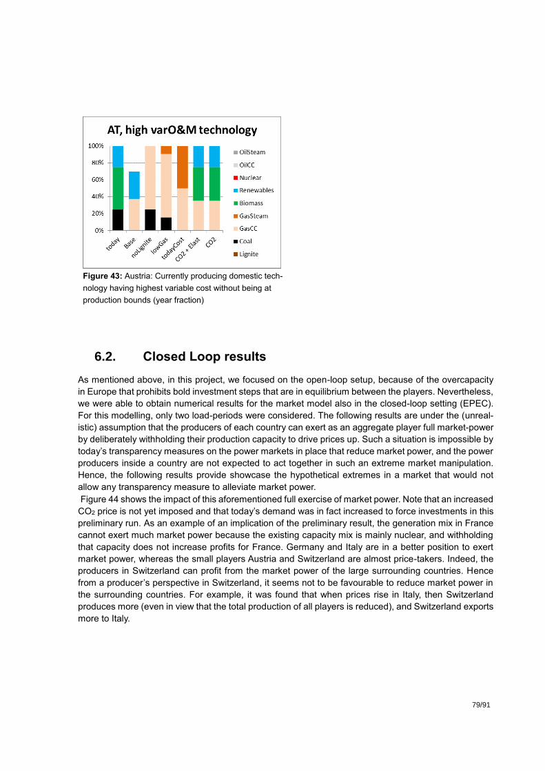
79/91
Figure 43: Austria: Currently producing domestic tech-
nology having highest variable cost without being at
production bounds (year fraction)
6.2. Closed Loop results
As mentioned above, in this project, we focused on the open-loop setup, because of the overcapacity
in Europe that prohibits bold investment steps that are in equilibrium between the players. Nevertheless,
we were able to obtain numerical results for the market model also in the closed-loop setting (EPEC).
For this modelling, only two load-periods were considered. The following results are under the (unreal-
istic) assumption that the producers of each country can exert as an aggregate player full market-power
by deliberately withholding their production capacity to drive prices up. Such a situation is impossible by
today’s transparency measures on the power markets in place that reduce market power, and the power
producers inside a country are not expected to act together in such an extreme market manipulation.
Hence, the following results provide showcase the hypothetical extremes in a market that would not
allow any transparency measure to alleviate market power.
Figure 44 shows the impact of this aforementioned full exercise of market power. Note that an increased
CO2 price is not yet imposed and that today’s demand was in fact increased to force investments in this
preliminary run. As an example of an implication of the preliminary result, the generation mix in France
cannot exert much market power because the existing capacity mix is mainly nuclear, and withholding
that capacity does not increase profits for France. Germany and Italy are in a better position to exert
market power, whereas the small players Austria and Switzerland are almost price-takers. Indeed, the
producers in Switzerland can profit from the market power of the large surrounding countries. Hence
from a producer’s perspective in Switzerland, it seems not to be favourable to reduce market power in
the surrounding countries. For example, it was found that when prices rise in Italy, then Switzerland
produces more (even in view that the total production of all players is reduced), and Switzerland exports
more to Italy.

Oligopolistic capacity expansion with subsequent market-bidding under transmission constraints (OCESM)
80/91
Figure 44: Influence of market power on price, profit and demand in the closed-loop model (Bi-
level nested game, EPEC). Reference (100%) is Social welfare (SW) maximisation. On the x-
axis (left to right): (i) SW maximisation; (ii) all players are price-takers on the market (second-
level),but all players still participate on the investment game (first-level); (iii) Germany has unre-
stricted market power on the market (second-level); (iv) Germany and France have unrestricted
market power, etc.
81/91
7. Auxiliary Analyses
In the course of the project, two auxiliary analyses were performed. The first analysis (master thesis)
investigated mainly correlation on the demand-side of the wholesale market, whereas the second anal-
ysis investigated a decomposition of wind and solar availability patterns. The analyses may be found
useful in extensions of the current project.
7.1. Empirical analysis of supply, price, and demand
In an empirical analysis, the elasticities of the demand curves at the EPEX market were investigated,
and correlations between marketed volumes, market prices and loads were analysed (within market
regions, and across regions). Moreover, a very detailed merit order for Germany was constructed and
compared with averaged bid-curves on the market. Details are presented below.
In an empirical analysis, the demand and price curves of the EPEX day-ahead spot market were inves-
tigated for recent years (most of the analysis is for 2015) and for the market areas Switzerland (CH),
France (FR), and Germany + Austria (DE+AT). In particular, the following dependencies were
investigated.
7.1.1. Price, Market volume, Demand
Price and (market-)volumes over a day. In all of the investigated market areas, the price for
each day-hour averaged over 2015 is considered:
High prices are observed in all areas approximately at 8 and 19 o’clock. On the other hand, the
variation in traded volumes over the day is different in different regions: In FR and CH, high vol-
umes are traded in the morning and the evening, whereas in DE+AT high volumes follow the PV
generation profile.
Price–Volume correlation inside a region. Daily (averaged) volumes and prices over the year
2015 were considered:
No correlation between price and volume could be detected. This contradicts traditional economic
analysis, which is not uncommon for power markets. In an extension, each hour of the day may be
investigated separately.
Price-Price correlation across regions. Daily (averaged) prices over the year 2015 were consid-
ered:
The highest correlation of (daily averaged) prices was observed between CH and FR, wherein a
regression model the R2-coefficient yielded 72%, whereas 33% were observed between CH and
DE+AT and 50% between FR and DE+AT. Clearly, this analysis should be further enhanced in an
extension by sub-setting the data points to winter/summer, peak/off-peak time.
Volume-Volume correlation across regions. The daily (averaged) volumes in the year 2014 were
only very weakly correlated across regions. A conjecture is that if a region produces more, the other
regions produce less, that is, they import (all other factors being constant), for example between CH
and FR. Note that the hourly profiles of CH and FR of traded volumes are nevertheless heavily
correlated (see above). Hence, further investigations may be of interest.

Oligopolistic capacity expansion with subsequent market-bidding under transmission constraints (OCESM)
82/91
Volume-Demand correlation inside a region. In a first analysis, the volume-demand correlation
was investigated on hourly historical data for 2015. Surprisingly, there is no high correlation in mar-
ket area CH and FR between demand and traded volume (for a specific hour). In DE+AT, a regres-
sion exhibited an R2-coefficient of 26%, which shows some correlation, which may be explained by
the higher share of demand traded in DE+AT (i.e., 46% in 2015, whereas only 23% in FR, and 37%
in CH).
In a second regression, the correlation was tested for each hour of the day in 2015 separately, and
no correlation was found at all. Hence, it seems that currently the market is used for additional short-
term trading, whereas the forecasted domestic demand of a supplier is covered beforehand off-
market, such that the (bulk) height of demand does not influence the additional trading.
7.1.2. Elasticities of demand-bids at EPEX
The elasticities of the (inverse) demand curves on the market were investigated. For this, the derivative
of the demand with respect to the price must be calculated approximatively. This is difficult for the ob-
served hourly (downward sloping) inverse demand curves, which are extremely steep at high prices for
low demands, then somehow linearly going down at moderate prices for many demand bids and then
going steep down again to negative prices for excess demand bids. In the master thesis, this problem
was tackled by taking logarithms (to tackle negative prices and because the elasticity is measured in
relative units), and with a line-search to find the (approximatively) linear part of the inverse demand
curve. The line searched started from the left of the inverse demand curve at a relatively high price of
70 EUR and searched for the successive pair of bids where the difference on the horizontal axes is
larger than 10 kWh, that is, where the downward slope starts to decrease. This bid defines (heuristically)
the start of the “linear” part until the realised price/volume pair, which is used as the right end-point of
the linear part. The 10 kWh and the 70 EUR where determined by heuristic trials. It was found that this
linear part is approximately 1 GWh for Switzerland and France markets, and 2 GW for Germany + Aus-
tria.
Elasticity-Elasticity correlation over time (auto-correlation) inside a region. The correlation of
the elasticity across chronological hours was evaluated in 2015. It could be shown that the correla-
tion of elasticity is very high in all market areas (FR, DE+AT, CH). Hence, it seems that the market
situation changes slowly on the demand side over following hours. In a possible extension, it would
be nice to evaluate the correlation between peak- and base-load hours (instead of chronological
hours).
Elasticity correlation across regions. The hourly 2015 data showed no significant correlation
between countries. Hence, it seems that the steepness of the demand bids on the markets is inde-
pendent and idiosyncratic for each market area.
Elasticity-Price correlation inside a region. For each of the 24 hours, the elasticities and prices
were averaged over all days of the year 2015. Highest elasticity was observed in the early morn-
ing in all market regions. Another important observed result is that prices and elasticities are nega-
tively correlated; see Figure 45.

83/91
Figure 45: Prices and demand elasticities, for each hour, averaged over the days of the year 2015, for each
region. Up/left: Switzerland, Up/right: Germany + Austria, Down: France.
A possible explanation for the inverse relationship is as follows: When prices are high, then volumes are
usually also high in the electricity markets. Hence, high volumes are demanded despite prices are high
during these hours, which is an anomaly in the traditional economy. In these hours, demand bids are
only placed if really necessary, and must be placed independently on benevolent price-signals, or in
other words, the demand elasticity is low. Hence, there seem to be opportunities for market power in
those hours. This shall be investigated further.
7.1.3. Empirical analysis of merit order curve of Germany
In an empirical analysis, a synthesized merit order curve of Germany for the year 2015 was compared
with the supply curve on the market. Because the share of traded electricity in the DE+AT market area
is relatively large, it is expected that a merit order curve may somehow “match” the supply curve of DE
in the absence of significant amounts of market power. First, this was investigated over a yearly average
by constructing
1. A merit order curve for Germany (Figure 46), taking into account:
o 1563 power plants
o Estimated variable costs, CO2 costs, fuel costs
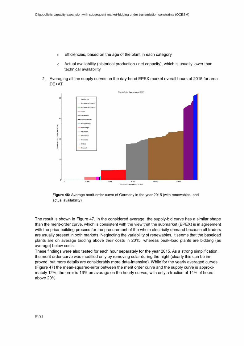
Oligopolistic capacity expansion with subsequent market-bidding under transmission constraints (OCESM)
84/91
o Efficiencies, based on the age of the plant in each category
o Actual availability (historical production / net capacity), which is usually lower than
technical availability
2. Averaging all the supply curves on the day-head EPEX market overall hours of 2015 for area
DE+AT.
Figure 46: Average merit-order curve of Germany in the year 2015 (with renewables, and
actual availability)
The result is shown in Figure 47. In the considered average, the supply-bid curve has a similar shape
than the merit-order curve, which is consistent with the view that the submarket (EPEX) is in agreement
with the price-building process for the procurement of the whole electricity demand because all traders
are usually present in both markets. Neglecting the variability of renewables, it seems that the baseload
plants are on average bidding above their costs in 2015, whereas peak-load plants are bidding (as
average) below costs.
These findings were also tested for each hour separately for the year 2015. As a strong simplification,
the merit order curve was modified only by removing solar during the night (clearly this can be im-
proved, but more details are considerably more data-intensive). While for the yearly averaged curves
(Figure 47) the mean-squared-error between the merit order curve and the supply curve is approxi-
mately 12%, the error is 16% on average on the hourly curves, with only a fraction of 14% of hours
above 20%.

85/91
Figure 47: Averaged supply curve and averaged merit order curve for Germany in
the year 2015. y-axis shows range [–80 ,100] EUR/MWh, with negative values set
to 0 EUR/MWh. Axes are scaled to 100%
7.2. Statistical decomposition of wind and solar availability
In a statistical analysis, the wind-solar power generation was decomposed to allow for low dimensional
scenario generations, which is a required approach to capture the intermittency of renewables in a
game-theoretic modelling, which is already numerically demanding per se. Details are presented below.
The underlying data for the statistical decomposition for the analysis was the solar and wind generation
profiles for Germany in 2012–2014. The original data source for the analysis was the open-source data-
provider EEXWATCH. The correlation between hourly solar and wind in 2012–2014 is shown in
Table 24, which exhibits the well-known pattern: Wind and solar are slightly negatively correlated, hence
they are slightly complementary power sources, and solar is correlated with demand, which alleviates
the disability to produce during nights. Figure 48 and Figure 49 show the availability over time: Whereas
solar has the usual bell-shaped pattern across all seasons, the wind is more prominent in the evening
or during nights (in winter), which contributes to the negative correlation with solar.
Table 24: Correlation between hourly data of solar power, wind power, and electricity demand in Germany during
2012–2014
Solar Wind Demand
Solar 1 -0.13 0.45
Wind 1 0.088
Demand 1

Oligopolistic capacity expansion with subsequent market-bidding under transmission constraints (OCESM)
86/91
Figure 48: Solar availability in 2012–2014 across
seasons
Figure 49: Wind availability in 2012–2014 across
seasons
Figure 50: Screeplot of principal compo-
nents of the (24+24)-variate series of
hourly wind and solar power generation
during a year
Figure 51: Factor of loadings of the first three principal compo-
nents of the (24+24)-variate series of hourly wind and solar power
generation during a year
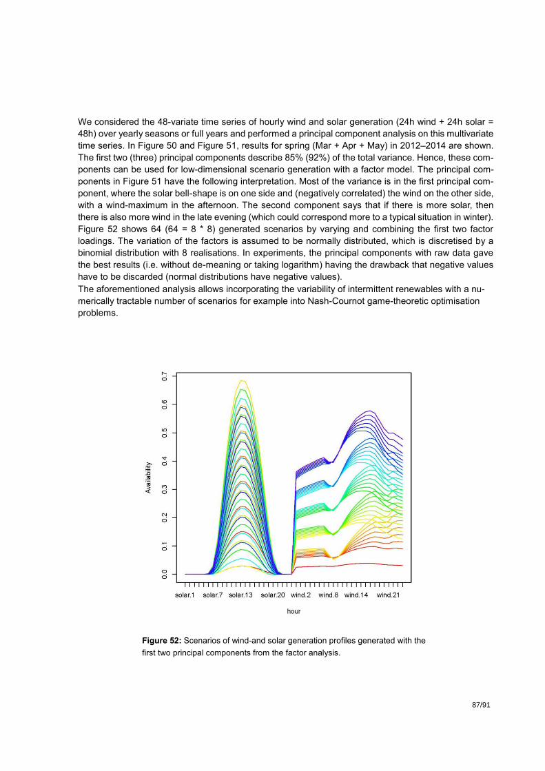
87/91
We considered the 48-variate time series of hourly wind and solar generation (24h wind + 24h solar =
48h) over yearly seasons or full years and performed a principal component analysis on this multivariate
time series. In Figure 50 and Figure 51, results for spring (Mar + Apr + May) in 2012–2014 are shown.
The first two (three) principal components describe 85% (92%) of the total variance. Hence, these com-
ponents can be used for low-dimensional scenario generation with a factor model. The principal com-
ponents in Figure 51 have the following interpretation. Most of the variance is in the first principal com-
ponent, where the solar bell-shape is on one side and (negatively correlated) the wind on the other side,
with a wind-maximum in the afternoon. The second component says that if there is more solar, then
there is also more wind in the late evening (which could correspond more to a typical situation in winter).
Figure 52 shows 64 (64 = 8 * 8) generated scenarios by varying and combining the first two factor
loadings. The variation of the factors is assumed to be normally distributed, which is discretised by a
binomial distribution with 8 realisations. In experiments, the principal components with raw data gave
the best results (i.e. without de-meaning or taking logarithm) having the drawback that negative values
have to be discarded (normal distributions have negative values).
The aforementioned analysis allows incorporating the variability of intermittent renewables with a nu-
merically tractable number of scenarios for example into Nash-Cournot game-theoretic optimisation
problems.
Figure 52: Scenarios of wind-and solar generation profiles generated with the
first two principal components from the factor analysis.

Oligopolistic capacity expansion with subsequent market-bidding under transmission constraints (OCESM)
88/91
8. Auxiliary Project Information
8.1. Dissemination
The work was presented at the following conferences and workshops:
Densing, M., Panos, E., Schmedders, K. (2015). Bi-level oligopolistic electricity market models: The case of Switzerland and surrounding countries, Conference for Operations Research (OR 2015), 1–4
Sept. 2015, University Vienna
Densing, M., Panos E., Schmedders, K. (2015). Decision making in electricity markets: Bi-level games and stochastic programming, Energy Science Centre Workshop, ETH Zurich,
https://www.psi.ch/eem/ConferencesTabelle/BilevelAndSP_MartinDensing_TALK.pdf
Densing, M., Panos, E., Schmedders, K. (2016). Bi-level oligopolistic electricity market models: The case of Switzerland and surrounding countries. Workshop at Faculty of Business and Economics, Uni-Basel. University of Basel (in cooperation with SFOE).
Densing, M., (2016). Oligopolistic Capacity Expansion with subsequent Market Bidding under Trans-mission constraints: Case of Switzerland and surrounding countries. Workshop „Econometric analysis of the determinants of electricity wholesale prices in Switzerland“. SFOE, Research programme En-
ergy-Economy-Society (EWG). ETH, Zurich.
Densing, M., Panos E. (2017). Stochastic bi-level electricity market modelling. SET-Nav WP10 Mod-
elling Forum. ETH Zurich.
Densing, M., Panos E. (2017). Modeling of electricity markets and hydropower dispatch. Swiss Com-petence Centres of Energy Research – Supply of Electricity (SCCER-SoE) Annual Conference, Bir-mensdorf (ZH), Swiss Federal Research Institute WSL
8.2. Personnel / Acknowledgment
The main staff on the project was: M. Densing, E. Panos, and K. Schmedders. The projected yielded
also a master thesis and an internship.
Christoph Groh (2016): Master thesis, University of Zürich. Stromhandel in der Schweiz und in
benachbarten Ländern – Analyse von Angebot und Nachfrage unter Benutzung eines Marktmo-
dells. The accomplished master thesis yields the basis for the data input of demand elasticities
and provides indications how prices and merit-order curves are correlated.
Jesus Lopez-Palacios (2017): Internship. Gathering data on electricity trade and wind and solar
generation for Switzerland and the surrounding countries.
We thank Dr. Robert Earle, visiting scientist at the Chair of Quantitative Business Administration, Uni-
versity of Zurich, for the helpful discussions, and the scientific staff at EPEX for their help. Finally the
various discussions with the SFOE, especially with Dr. Florian Kämpfer and Dr. Aurelio Fetz, helped to
improve the project considerably.

89/91
9. References
BFE / Prognos (2012). Energieperspektiven 2050. http://www.bfe.admin.ch/the-
men/00526/00527/06431/index.html?lang=de&dossier_id=06421
BFE(2016). Schweizerische Elektrizitätstatistik. http://www.bfe.admin.ch/the-
men/00526/00541/00542/00630/index.html?dossier_id=00765
Bundesnetzagentur (2017). Kraftwerksliste, Deutschland. https://www.bundesnetzagen-tur.de/DE/Sachgebiete/ElektrizitaetundGas/Unternehmen_Institutionen/Versorgungssicherheit/Erzeu-gungskapazitaeten/Kraftwerksliste/kraftwerksliste.html
Chen, Y., Sijm, J., Hobbs, BF., Lise, W. (2008). Implications of CO2 emissions trading for short-run electricity market outcomes in northwest Europe, Journal of Regulatory Economics, 34, pp. 251-281. DOI: 10.1007/s11149-008-9069-9
Cournot, A. (1838). Recherches sur les principes mathématiques de la théorie des richesses, Paris.
Corts, K. (1999). Conduct parameters and the measurement of market power, 88, p. 227-250, Journal of Econometrics.
Densing, M. (2013). Price-driven hydropower dispatch under uncertainty, in R. M. Kovacevic, G. C. Pflug & M. T. Vespucci, eds, ‘Handbook of Risk Management in Energy Production and Trading’, Vol. 199 of Int. Series in Operations Research & Management Science, Springer, pp. 73–104.
Densing, M., Panos, E., Schmedders, K. (2015). Bi-level oligopolistic electricity market models: The case of Switzerland and surrounding countries, Conference for Operations Research (OR 2015), 1–4
Sept. 2015, University Vienna
Densing, M., Panos E., Schmedders, K. (2015). Decision making in electricity markets: Bi-level games and stochastic programming, Energy Science Center Workshop, ETH Zurich, https://www.psi.ch/eem/ConferencesTabelle/BilevelAndSP_MartinDensing_TALK.pdf
Dirkse, S., Ferris, M. (1995). The path solver: a non-monotone stabilization scheme for mixed com-plementarity problems, Optimisation Methods and Software 5:2. DOI: 10.1080/10556789508805606
E-CONTROL (2017). https://www.e-control.at/en/
Energate Messenger (2017): Energate Mssenger Schweiz: Energie-Nachrichten für die Schweiz.
Marktdaten. www.energate-messenger.ch
ENTSO-E (2015): Transparency platform. FTP-download. https://transparency.entsoe.eu/
EU (2017). European Commission, Energy Modelling, EU Reference Scenario 2016 & EUCO scena-
rios. https://ec.europa.eu/energy/en/data-analysis/energy-modelling
EPEX (2017). European Electricity Exchange. Market data feed. https://www.epexspot.com/
Filippini, M., Geissmann, T. (2014). Kostenstruktur und Kosteneffizienz der Schweizer Wasserkraft.
Erstellt im Auftrag des Bundesamtes für Energie (BFE).
Gabriel, S., et al. (2013). Complementarity Modeling in Energy Markets, Springer. DOI: 10.1007/978-
1-4419-6123-5
GME (2017). Gestore dei Mercati Energetici SpA. Market data feed. www.mercatoelettrico.org

Oligopolistic capacity expansion with subsequent market-bidding under transmission constraints (OCESM)
90/91
Groh, C. (2016): Stromhandel in der Schweiz und in benachbarten Ländern – Analyse von Angebot und Nachfrage unter Benutzung eines Marktmodells, Master Thesis at Institut für Betriebswirtschafts-lehre, Universität Zürich (in press; pdf-version available on request)
Lagarto, J., Sousa, J., Martins, A., Ferrao, P. (2014). Market power analysis in the Iberian electricity market using a conjectural variations model, Energy, 76, pp.292-305. DOI: 10.1016/j.en-ergy.2014.08.014
Lise, W., Sijm, J., Hobbs, BF. (2010). The impact of EU ETS on prices, profits and emissions in the power sector: simulations results with the COMPETE EU20 Model, Environmental and Resource Eco-nomics, 47, pp. 23-44. DOI: 10.1007/s10640-010-9362-9
Kouvaritakis, N., Panos, V. (2004). Modelling the impact of emissions trading in Greek Electricity Sector – Application of ELMAS model, Technical Report to European Commission for the project ETRES (LIFE03/ENV/GR/000219), E3M Lab, National Technical University of Athens.
Metzler, C., Hobbs, B., Pang, J.(2003). Nash-Cournot Equilibria in Power Markets on a Linearized DC Network with Arbitrage: Formulations and Properties, Networks and Spatial Economics, 3(2), 123-150, DOI 10.1023/a:1023907818360
OECD / IEA (2013): Net Capacity of renewables. DOI: 10.1787/data-00467-en.
http://wds.iea.org/WDS/tableviewer/document.aspx?FileId=1519
JRC (Simoes, S., Nijs, W., Ruiz, P., Sgobbi, A., Radu, D., Bolat, P., Thiel, C. & Peteves, S.) (2013). The JRC-EU-TIMES model. European Commission DOI: 10.2790/97596
DIW (Schröder, A., Kunz, F., Meiss, J., Mendelevitch, R., von Hirschhausen, C.) (2013). Current and Prospective Costs of Electricity Generation until 2050. Deutsches Institut für Wirtschaftsforschung (DIW). https://www.diw.de/documents/publikationen/73/diw_01.c.424566.de/diw_datadoc_2013-068.pdf
Panos, E., Lehtila, A. (2016). Dispatching and unit commitment features in TIMES. International En-ergy Agency – Energy Technology Systems Analysis Program (ETSAP). https://iea-etsap.org/pro-jects/TIMES_Dispatching_Documentation.pdf
Palmintier, B., (2014). Flexibility in generation planning: Identifying key operating constratins, in: Power Systems Computation Conference (PSCC), Wroclaw, Poland. DOI: 10.1109/PSCC.2014.7038323
PCR (2016). Price Coupling of Regions. Description of market coupling algorithm. https://www.nord-
poolspot.com/globalassets/download-center/pcr/euphemia-public-documentation.pdf
PSI (2017). Eds. Hirschberg, S., Bauer., C. Potentials, costs and environmental assessment of elec-
tricity generation technologies (in press)
Ralph, D. (1994). Global convergence of damped Newton’s method for nonsmooth equations via the
path search, Mathematics of Operations Research 19(2). DOI: 10.1287/moor.19.2.352
SWV (2012/2016). Heimfall und Neukonzessionierung von Wasserkraftwerken, Faktenblatt November
2012. Schweizerischer Wasserwirtschaftsverband.
Van Stiphout, A., De Vos, K., Deconinck, G. (2016). The impact of operating reserves on investment planning of renewable power systems, IEEE Transactions on Power Systems. 99. DOI: 10.1109/TPWRS.2016.2565058
WEO (2016). World Energy Outlook. ISBN Print: 978-92-64-26494-6 / PDF: 978-92-64-26495-3. https://www.iea.org/bookshop/720-World_Energy_Outlook_2016

91/91
Wogrin, S., Centeno, E., Barquin, J. (2013). Generation Capacity Expansion Analysis: Open Loop Approximation of Closed Loop Equilibria, IEEE Transactions on Power Systems. 28(3), pp. 3362—3371. DOI: 10.1109/tpwrs.2013.2252632