oligopoly thoery1 oligopoly theory (8) product differentiation and spatial competition aim of this...
TRANSCRIPT
Oligopoly Thoery 1
Oligopoly Theory (8)Product Differentiation and Spatial
Competition
Aim of this lecture(1) To understand the relationship between product
differentiation and locations of the firms. (2) To understand the difference between mill
pricing and delivered pricing.
Oligopoly Thoery 2
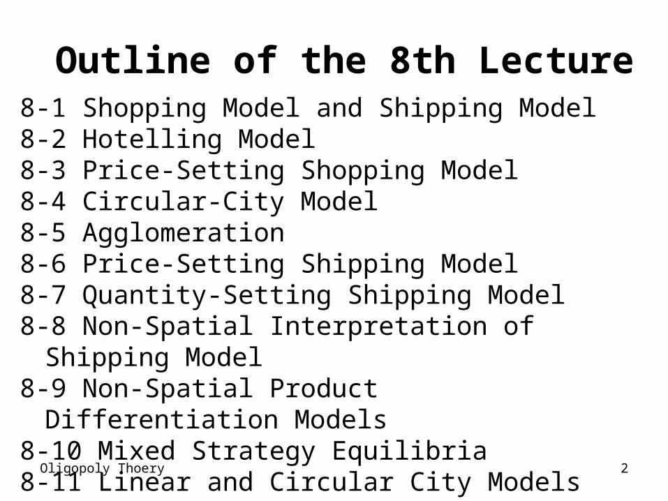
Outline of the 8th Lecture8-1 Shopping Model and Shipping Model 8-2 Hotelling Model8-3 Price-Setting Shopping Model8-4 Circular-City Model 8-5 Agglomeration8-6 Price-Setting Shipping Model8-7 Quantity-Setting Shipping Model 8-8 Non-Spatial Interpretation of Shipping
Model 8-9 Non-Spatial Product Differentiation
Models 8-10 Mixed Strategy Equilibria8-11 Linear and Circular City Models Revisited
Oligopoly Thoery 3
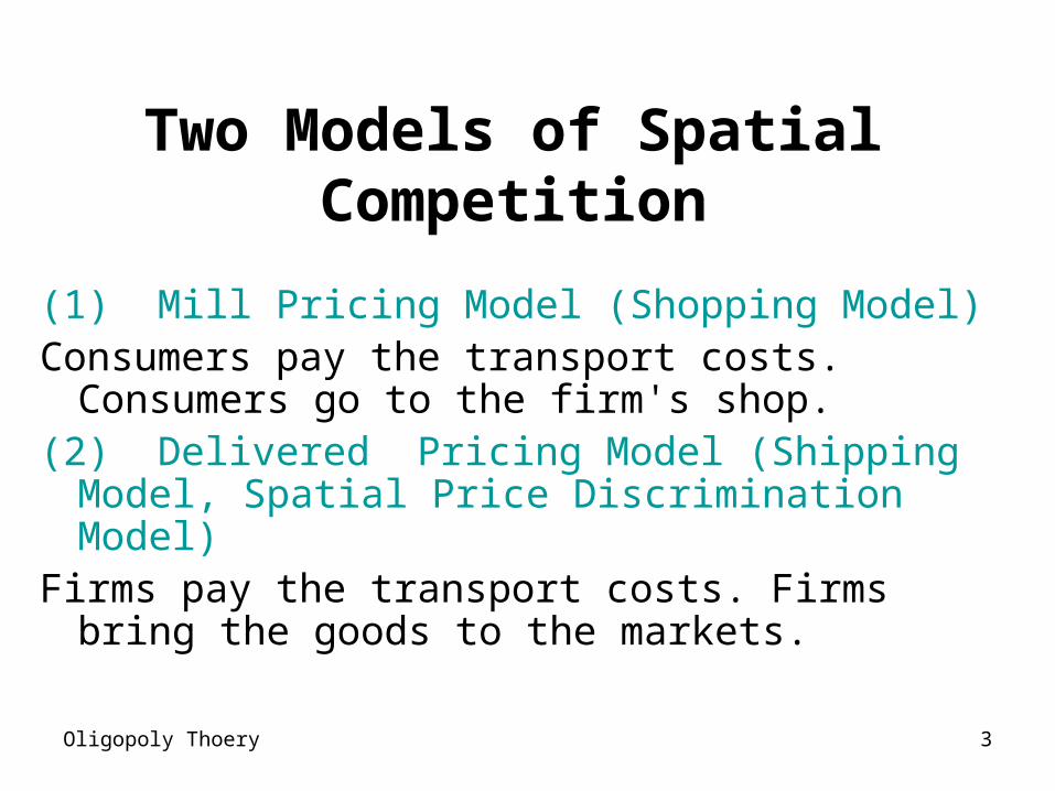
Two Models of Spatial Competition
(1) Mill Pricing Model (Shopping Model)Consumers pay the transport costs. Consumers go
to the firm's shop.(2) Delivered Pricing Model (Shipping Model,
Spatial Price Discrimination Model)Firms pay the transport costs. Firms bring the goods
to the markets.
Oligopoly Thoery 4
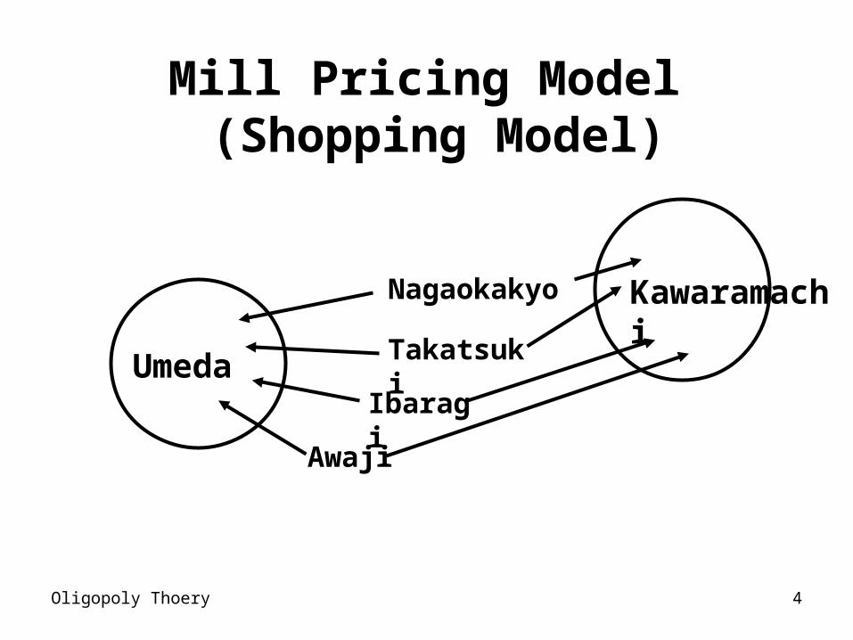
Mill Pricing Model (Shopping Model)
Kawaramachi
Umeda
Awaji
Ibaragi
Nagaokakyo
Takatsuki

Oligopoly Thoery 5
Mill Pricing Model (Shopping Model)
Kichijoji
Tachikawa
Kunitachi
Kokubunji
Mitaka
Musashisakai
Oligopoly Thoery 6
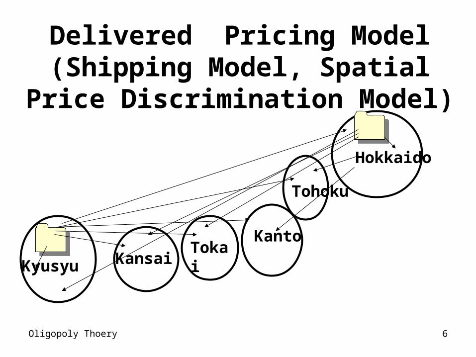
Delivered Pricing Model (Shipping Model, Spatial Price Discrimination
Model)
Hokkaido
Kyusyu KansaiTokai
Tohoku
Kanto
Oligopoly Thoery 7
Mill Pricing (Shopping) Models
Oligopoly Thoery 8
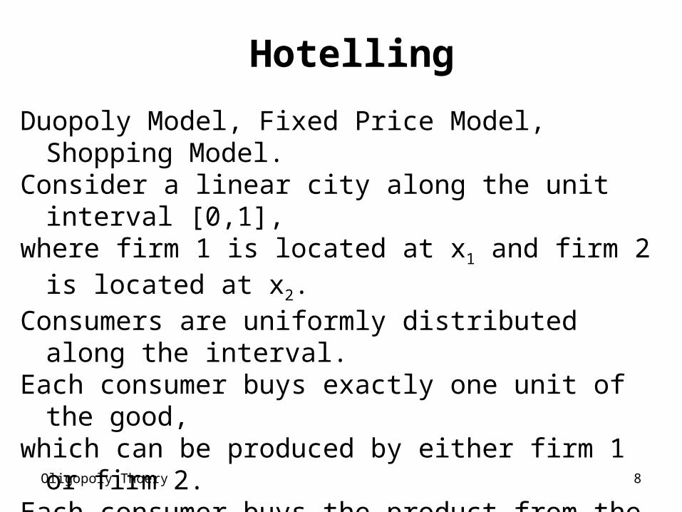
Hotelling
Duopoly Model, Fixed Price Model, Shopping Model.
Consider a linear city along the unit interval [0,1],where firm 1 is located at x1 and firm 2 is located at x2.Consumers are uniformly distributed along the
interval.Each consumer buys exactly one unit of the good,which can be produced by either firm 1 or firm 2.Each consumer buys the product from the firm
that is closer to her. Each firm chooses its location independently.
Oligopoly Thoery 9
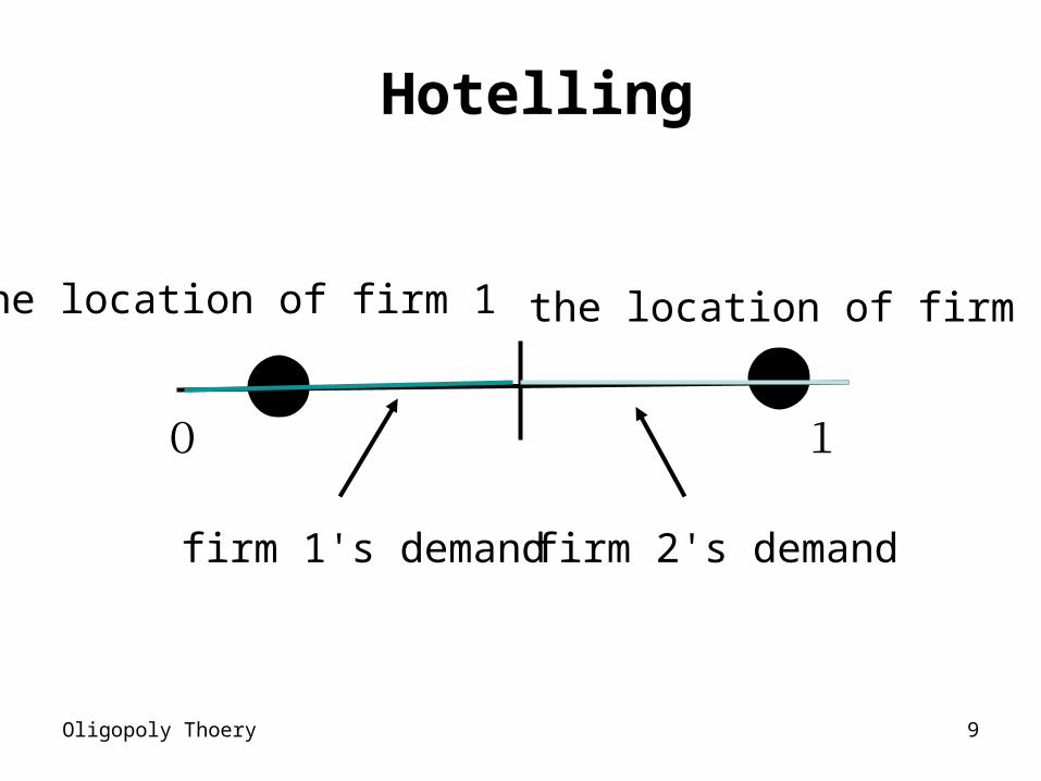
Hotelling
0 1
the location of firm 1 the location of firm 2
firm 1's demand firm 2's demand
Oligopoly Thoery 10
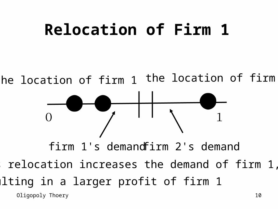
Relocation of Firm 1
0 1
the location of firm 1 the location of firm 2
firm 1's demand firm 2's demand
This relocation increases the demand of firm 1,
resulting in a larger profit of firm 1
Oligopoly Thoery 11
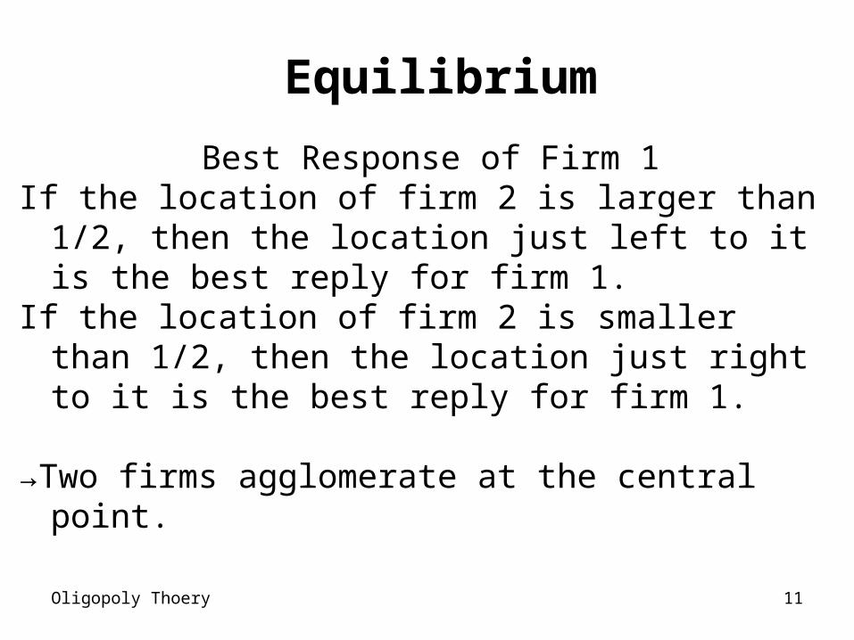
Equilibrium
Best Response of Firm 1If the location of firm 2 is larger than 1/2, then
the location just left to it is the best reply for firm 1.
If the location of firm 2 is smaller than 1/2, then the location just right to it is the best reply for firm 1.
→Two firms agglomerate at the central point.

Oligopoly Thoery 12
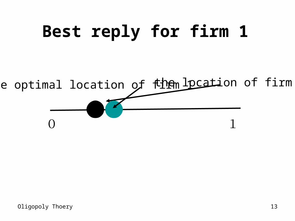
Best reply for firm 1
0 1
the optimal location of firm 1 the location of firm 2
Oligopoly Thoery 13
Best reply for firm 1
0 1
the optimal location of firm 1 the location of firm 2
Oligopoly Thoery 14
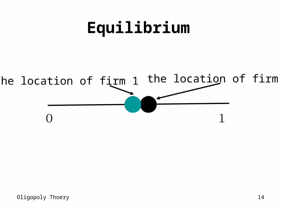
Equilibrium
0 1
the location of firm 1 the location of firm 2
Oligopoly Thoery 15
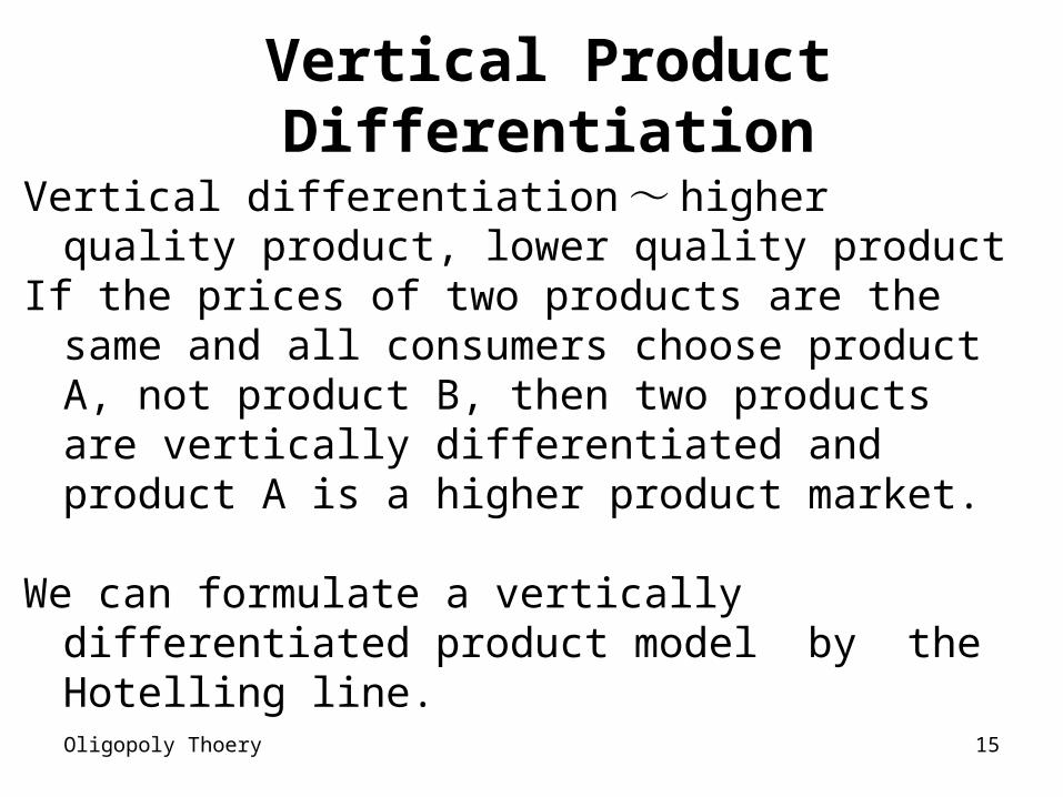
Vertical Product Differentiation
Vertical differentiation ~ higher quality product, lower quality product
If the prices of two products are the same and all consumers choose product A, not product B, then two products are vertically differentiated and product A is a higher product market.
We can formulate a vertically differentiated product model by the Hotelling line.
Oligopoly Thoery 16
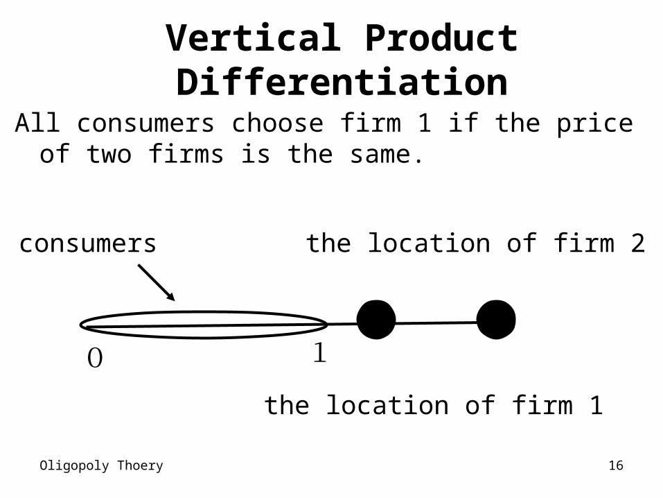
Vertical Product Differentiation
All consumers choose firm 1 if the price of two firms is the same.
0 1
the location of firm 1
the location of firm 2consumers
Oligopoly Thoery 17
Interpretation of the linear city
(1) city ~ spatial interpretation(2) product differentiation ~ horizontal product
differentiation(3) political preference
(3)→interpretation of minimal differentiation~ The policies of two major parties become similar.
However, following the interpretation of (1) and (2), the model lacks the reality since consumers care about prices as well as the locations of the firms.
Oligopoly Thoery 18
Endogenous Price
Duopoly Model, Shopping Model. Consider a linear city along the unit interval [0,1], where firm 1 is located at x1 and firm 2 is located at x2.
Consumers are uniformly distributed along the interval. Each consumer buys exactly one unit of the good, which can be produced by either firm 1 or firm 2. Each consumer buys the product from the firm whose real price (price +transport cost) is lower.

Oligopoly Thoery 19
One-Stage Location-Price Model
Duopoly Model, Shopping Model. Consider a linear city along the unit interval [0,1], where firm 1 is located at x1 and firm 2 is located at x2.
Consumers are uniformly distributed along the interval. Each consumer buys exactly one unit of the good, which can be produced by either firm 1 or firm 2. Each consumer buys the product from the firm whose real price (price + transport cost) is lower.
Each firm chooses its location and price independently.
Oligopoly Thoery 20
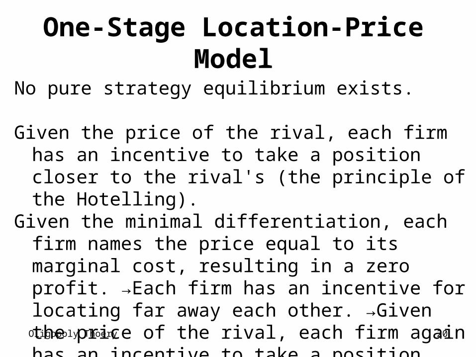
One-Stage Location-Price Model
No pure strategy equilibrium exists.
Given the price of the rival, each firm has an incentive to take a position closer to the rival's (the principle of the Hotelling).
Given the minimal differentiation, each firm names the price equal to its marginal cost, resulting in a zero profit. →Each firm has an incentive for locating far away each other. →Given the price of the rival, each firm again has an incentive to take a position closer to the rival's (the principle of the Hotelling).
Oligopoly Thoery 21
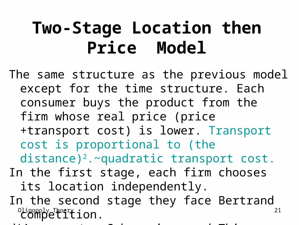
Two-Stage Location then Price Model
The same structure as the previous model except for the time structure. Each consumer buys the product from the firm whose real price (price +transport cost) is lower. Transport cost is proportional to (the distance)2.~quadratic transport cost.
In the first stage, each firm chooses its location independently.
In the second stage they face Bertrand competition.
d'Aspremont, Gabszewics, and Thisse, (1979, Econometrica)
Oligopoly Thoery 22
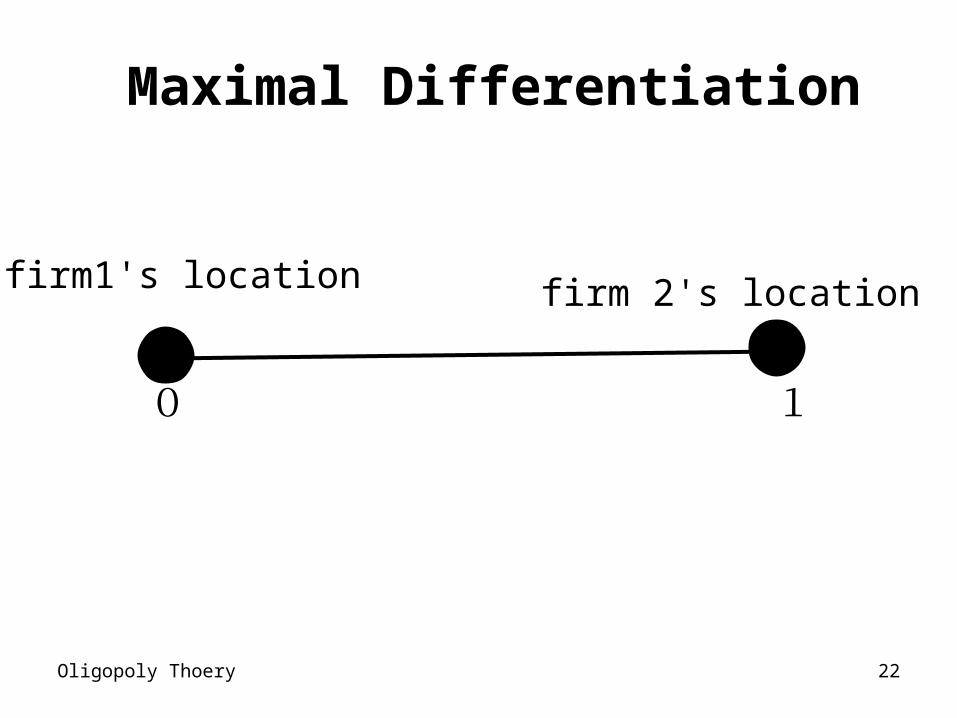
Maximal Differentiation
0 1
firm1's location firm 2's location
Oligopoly Thoery 23
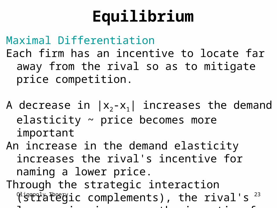
Equilibrium
Maximal DifferentiationEach firm has an incentive to locate far away
from the rival so as to mitigate price competition.
A decrease in |x2-x1| increases the demand elasticity ~ price becomes more important
An increase in the demand elasticity increases the rival's incentive for naming a lower price.
Through the strategic interaction (strategic complements), the rival's lower price increases the incentive for naming a lower price.→further reduction of the rival's price
Oligopoly Thoery 24
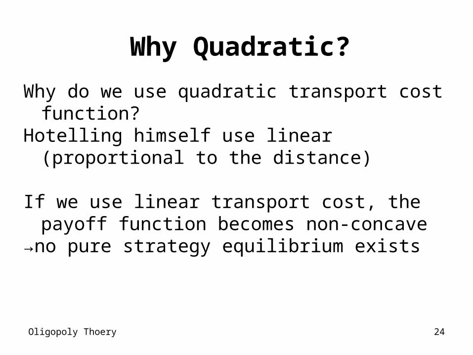
Why Quadratic?
Why do we use quadratic transport cost function?
Hotelling himself use linear (proportional to the distance)
If we use linear transport cost, the payoff function becomes non-concave
→no pure strategy equilibrium exists
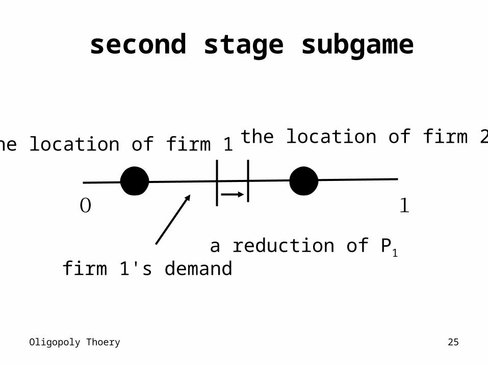
Oligopoly Thoery 25
second stage subgame
0 1
the location of firm 1 the location of firm 2
firm 1's demanda reduction of P1
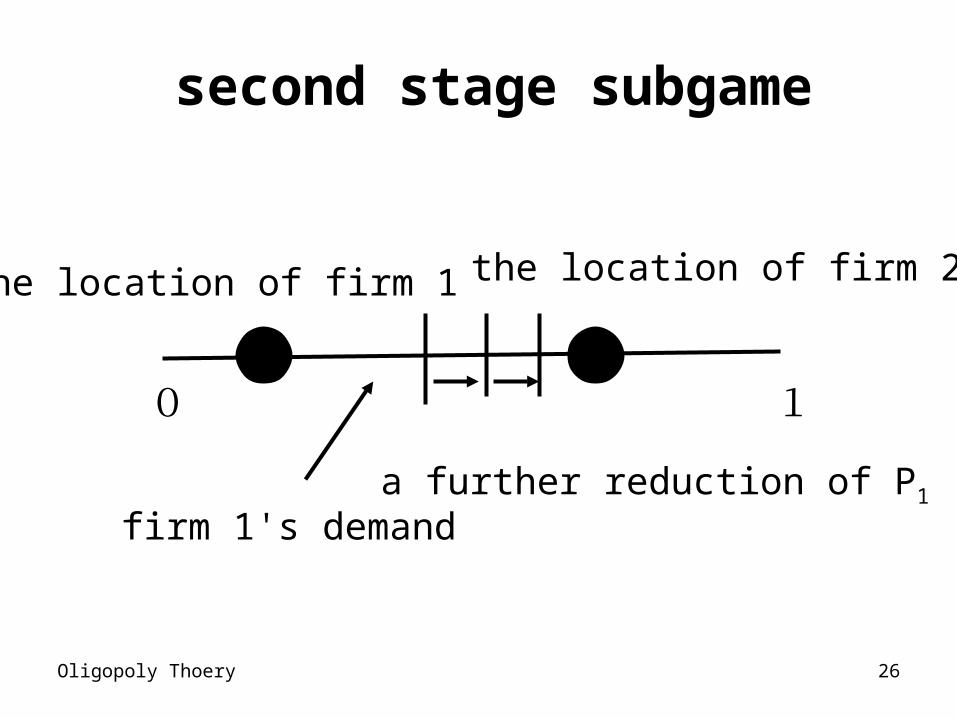
Oligopoly Thoery 26
second stage subgame
0 1
the location of firm 1 the location of firm 2
firm 1's demanda further reduction of P1
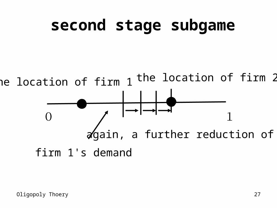
Oligopoly Thoery 27
second stage subgame
0 1
the location of firm 1 the location of firm 2
firm 1's demand
again, a further reduction of P1
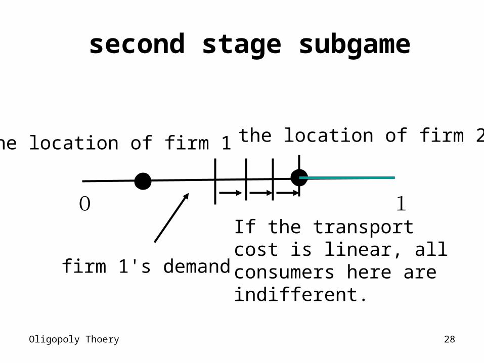
Oligopoly Thoery 28
second stage subgame
0 1
the location of firm 1 the location of firm 2
firm 1's demand
If the transport cost is linear, all consumers here are indifferent.
Oligopoly Thoery 29
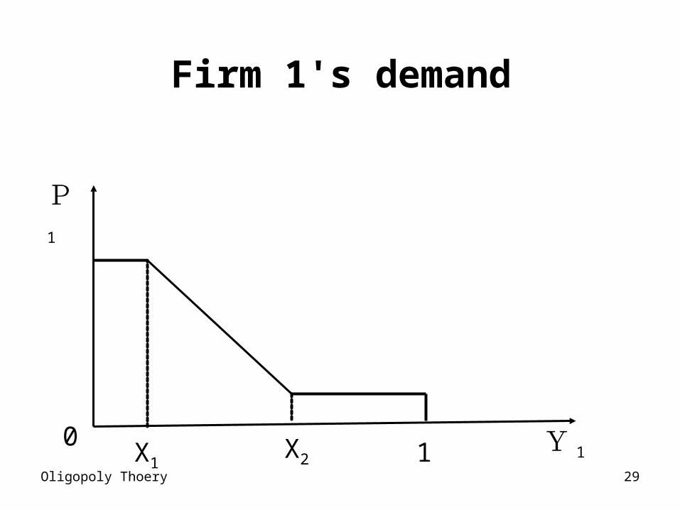
Firm 1's demand
P1
Y 10 X2X1 1
Oligopoly Thoery 30
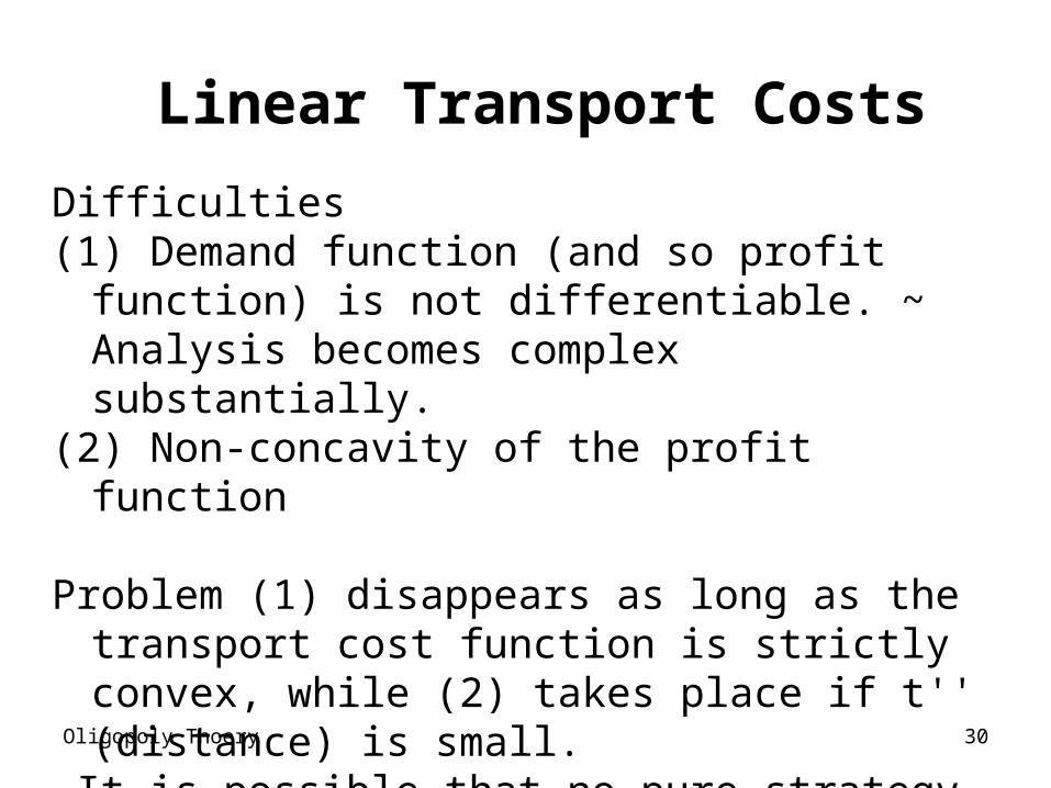
Linear Transport Costs
Difficulties(1) Demand function (and so profit function)
is not differentiable. ~ Analysis becomes complex substantially.
(2) Non-concavity of the profit function
Problem (1) disappears as long as the transport cost function is strictly convex, while (2) takes place if t'' (distance) is small.
→It is possible that no pure strategy equilibrium exists even when t'' >0.
Oligopoly Thoery 31
Strong ConvexityDifficulty when t'' is too large. If t'' is too large, given the moderate price p2,
firm 1 can monopolize the market near to its location. Thus, it has an incentive to name a high price and obtains the market near to its location only.
→Given this high price, firm 2 raises the price→Given firm 2's high price, firm 1 reduces the
price substantially and obtains a larger market.
→Given firm 1's low price, firm 2 has an incentive to raise the price and obtain the market near to its location only. →firm 1 raises the price.
~ similar to Edgeworth Cycle.
Oligopoly Thoery 32
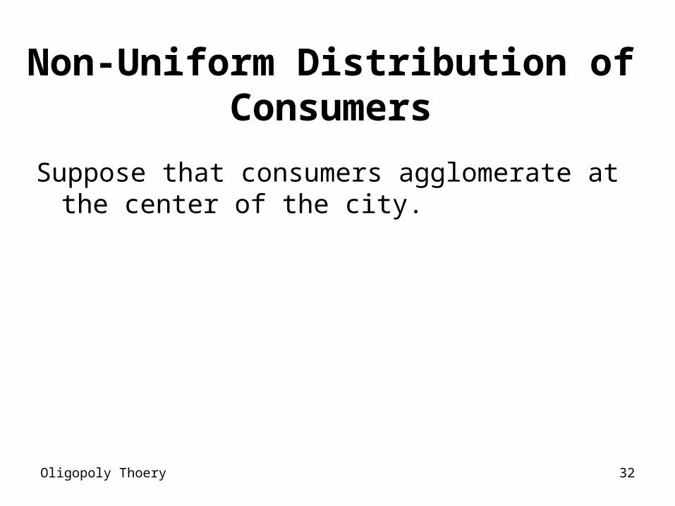
Non-Uniform Distribution of Consumers
Suppose that consumers agglomerate at the center of the city.
Oligopoly Thoery 33
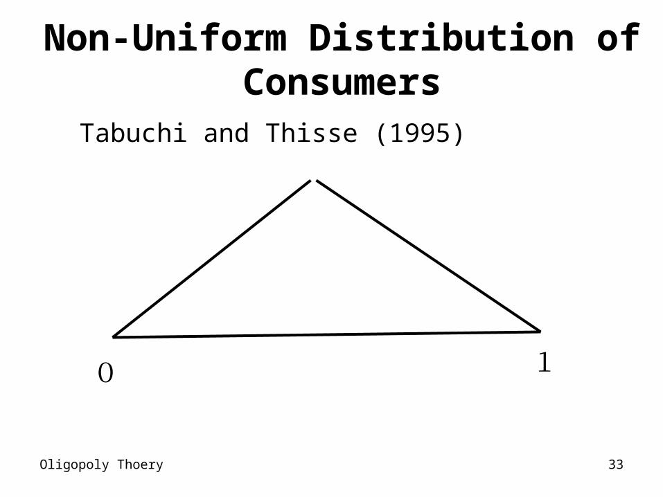
Non-Uniform Distribution of Consumers
0 1
Tabuchi and Thisse (1995)
Oligopoly Thoery 34
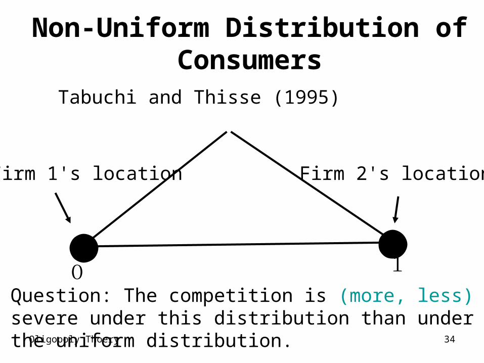
Non-Uniform Distribution of Consumers
0 1
Tabuchi and Thisse (1995)
Firm 1's location Firm 2's location
Question: The competition is (more, less) severe under this distribution than under the uniform distribution.
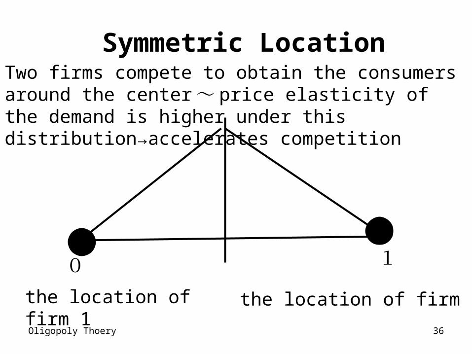
Oligopoly Thoery 35
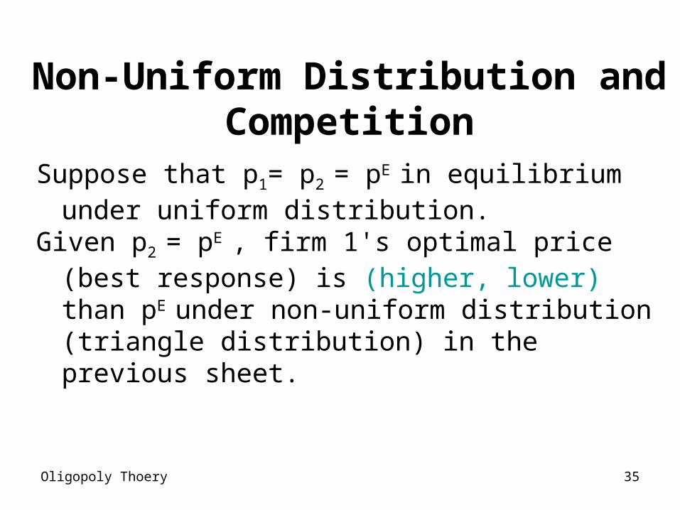
Non-Uniform Distribution and Competition
Suppose that p1= p2 = pE in equilibrium under uniform distribution.
Given p2 = pE , firm 1's optimal price (best response) is (higher, lower) than pE under non-uniform distribution (triangle distribution) in the previous sheet.
Oligopoly Thoery 36
Symmetric Location
0 1
the location of firm 1
the location of firm 2
Two firms compete to obtain the consumers around the center ~ price elasticity of the demand is higher under this distribution→accelerates competition
Oligopoly Thoery 37
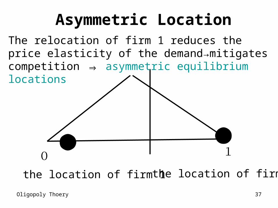
Asymmetric Location
0 1
the location of firm 1 the location of firm 2
The relocation of firm 1 reduces the price elasticity of the demand→mitigates competition ⇒ asymmetric equilibrium locations
Oligopoly Thoery 38
Two-Dimension Space
Oligopoly Thoery 39
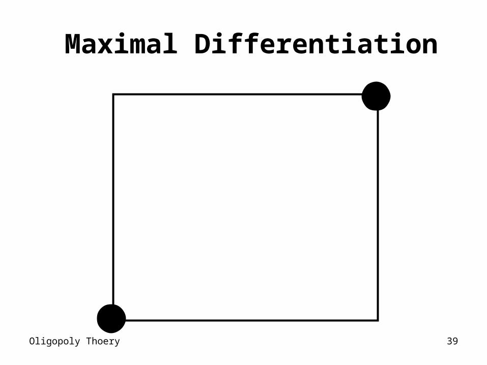
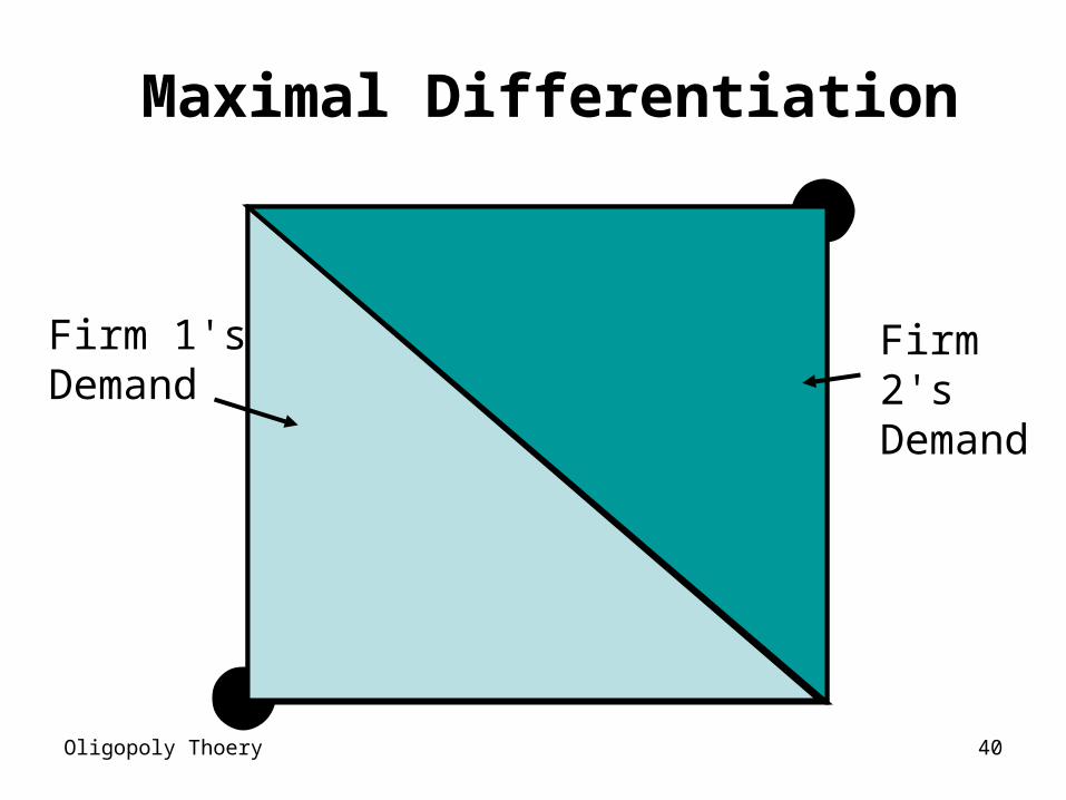
Maximal Differentiation
Oligopoly Thoery 40
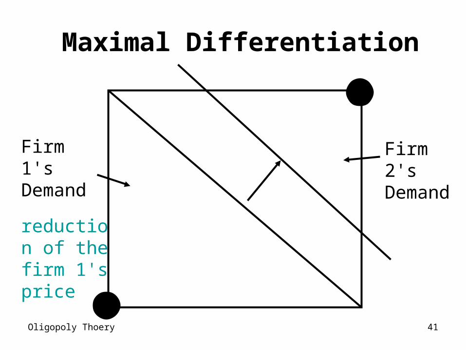
Maximal Differentiation
Firm 1's Demand
Firm 2's Demand
Oligopoly Thoery 41
Maximal Differentiation
Firm 1's Demand
Firm 2's Demand
reduction of the firm 1's price
Oligopoly Thoery 42
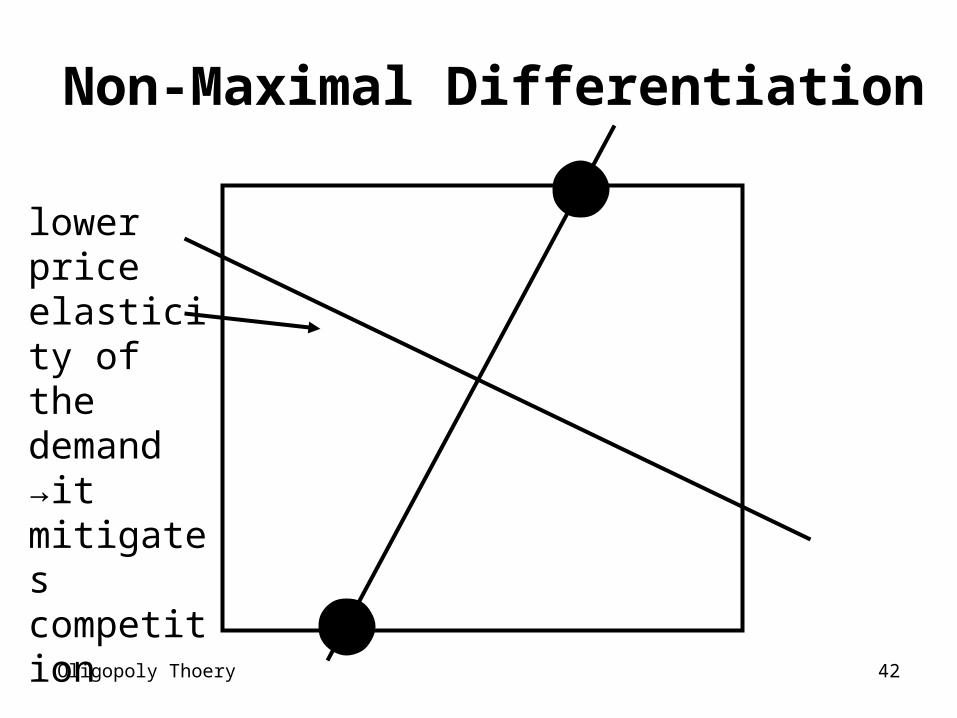
Non-Maximal Differentiation
lower price elasticity of the demand→it mitigates competition
Oligopoly Thoery 43
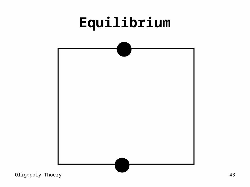
Equilibrium
Oligopoly Thoery 44
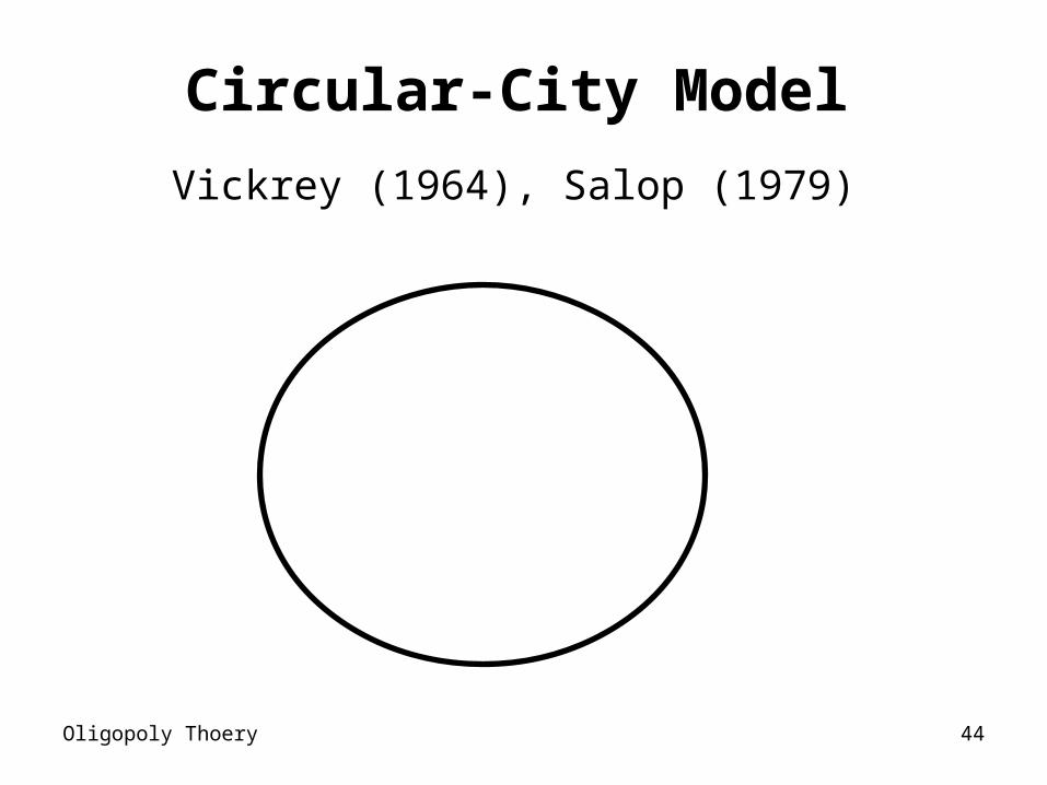
Circular-City Model
Vickrey (1964), Salop (1979)
Oligopoly Thoery 45
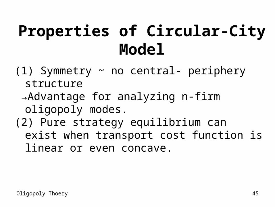
Properties of Circular-City Model
(1) Symmetry ~ no central- periphery structure
→Advantage for analyzing n-firm oligopoly modes.
(2) Pure strategy equilibrium can exist when transport cost function is linear or even concave.
Oligopoly Thoery 46
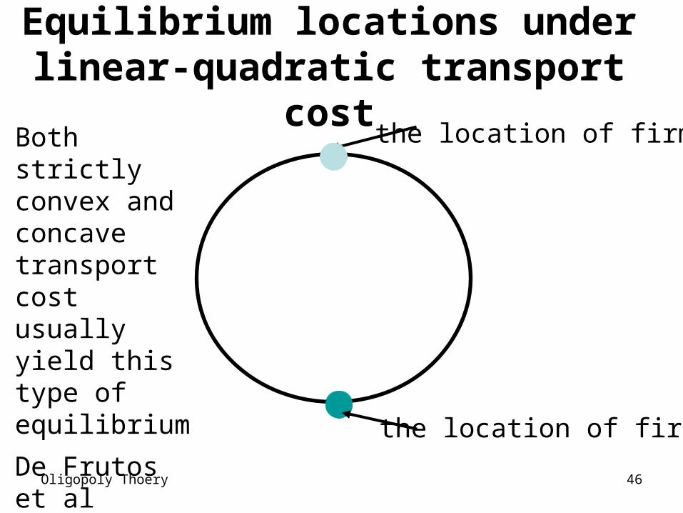
Equilibrium locations under linear-quadratic transport cost
the location of firm 1
the location of firm 2
Both strictly convex and concave transport cost usually yield this type of equilibrium
De Frutos et al (1999,2002)
Oligopoly Thoery 47
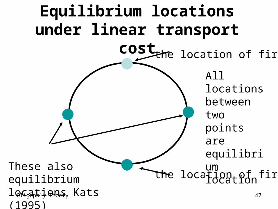
Equilibrium locations under linear transport cost
the location of firm 1
the location of firm 2These also equilibrium locations Kats (1995)
All locations between two points are equilibrium location
Oligopoly Thoery 48
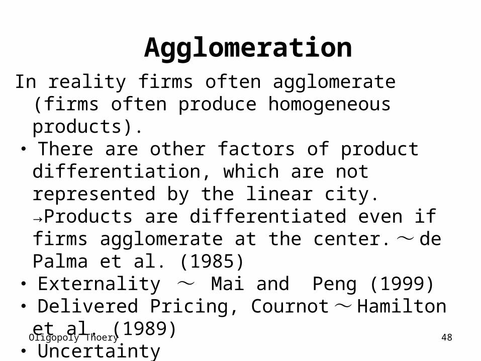
AgglomerationIn reality firms often agglomerate (firms often produce
homogeneous products).・ There are other factors of product differentiation,
which are not represented by the linear city. →Products are differentiated even if firms agglomerate at the center. ~ de Palma et al. (1985)
・ Externality ~ Mai and Peng (1999)・ Delivered Pricing, Cournot ~ Hamilton et al.
(1989)・ Uncertainty・ Location then Collusion・ Cost Asymmetry
Oligopoly Thoery 49
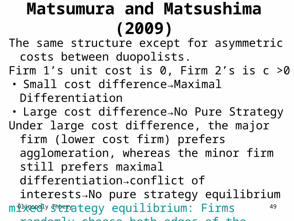
Matsumura and Matsushima (2009)The same structure except for asymmetric costs
between duopolists.Firm 1’s unit cost is 0, Firm 2’s is c >0・ Small cost difference→Maximal Differentiation・ Large cost difference→No Pure StrategyUnder large cost difference, the major firm (lower cost
firm) prefers agglomeration, whereas the minor firm still prefers maximal differentiation→conflict of interests→No pure strategy equilibrium
mixed strategy equilibrium: Firms randomly choose both edges of the city→agglomeration with probability ½.
Oligopoly Thoery 50
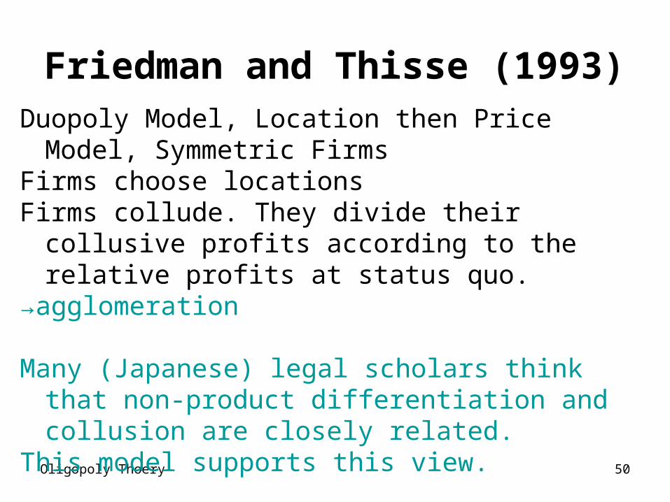
Friedman and Thisse (1993) Duopoly Model, Location then Price Model,
Symmetric FirmsFirms choose locationsFirms collude. They divide their collusive profits
according to the relative profits at status quo. →agglomeration
Many (Japanese) legal scholars think that non-product differentiation and collusion are closely related.
This model supports this view.

Oligopoly Thoery 51
Intuition behind agglomeration Firm 1 moves from the edge to the center →Its profit
decreases and the rival’s profit also decreasesIts own profit ~ Hotelling effect (positive)+
competition accelerate effect (negative)Rival's profit ~ Hotelling effect (negative)+
competition accelerate effect (negative)→improves bargaining position of firm 1.This is why agglomeration appears in location-
collusion model.
Oligopoly Thoery 52
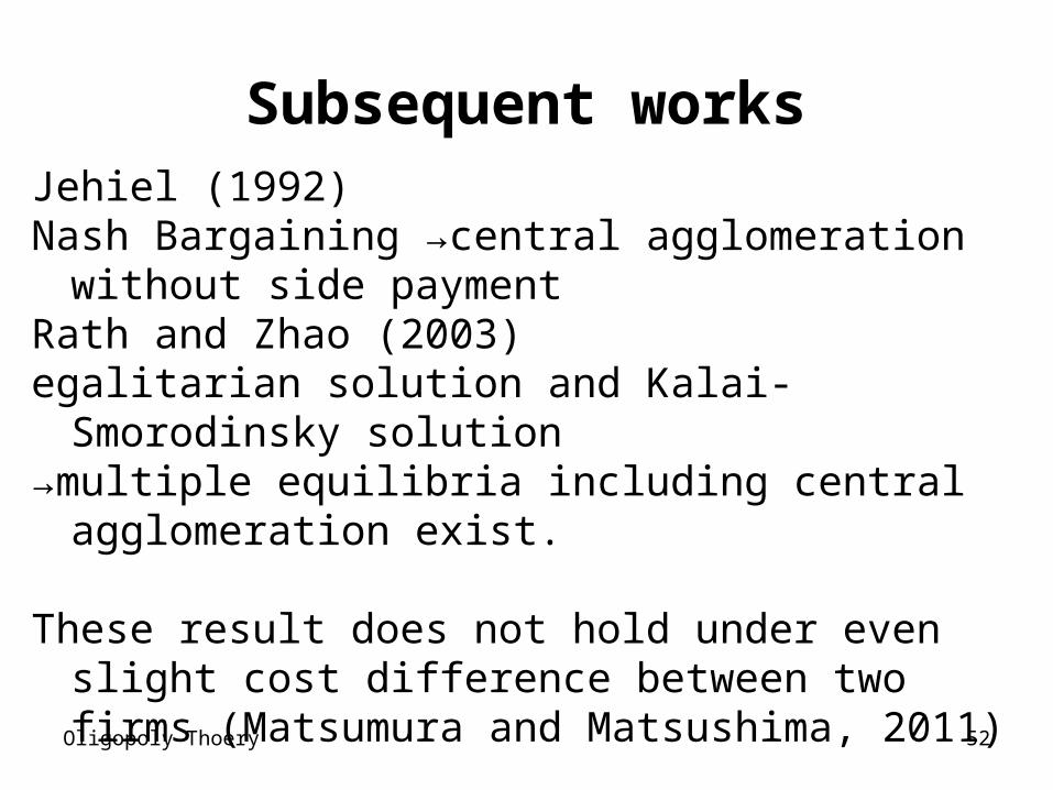
Subsequent works Jehiel (1992) Nash Bargaining →central agglomeration without
side paymentRath and Zhao (2003) egalitarian solution and Kalai-Smorodinsky solution→multiple equilibria including central agglomeration
exist.
These result does not hold under even slight cost difference between two firms (Matsumura and Matsushima, 2011)
Oligopoly Thoery 53
Delivered Pricing (Shipping) Models
Oligopoly Thoery 54
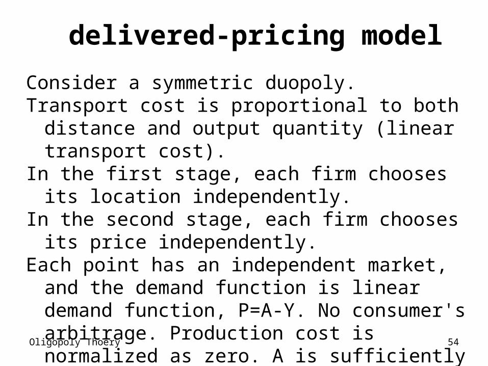
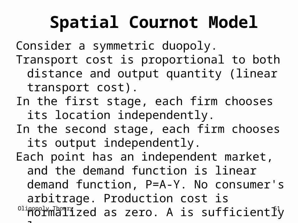
delivered-pricing model
Consider a symmetric duopoly. Transport cost is proportional to both distance
and output quantity (linear transport cost). In the first stage, each firm chooses its
location independently.In the second stage, each firm chooses its
price independently.Each point has an independent market, and
the demand function is linear demand function, P=A-Y. No consumer's arbitrage. Production cost is normalized as zero. A is sufficiently large.
Oligopoly Thoery 55
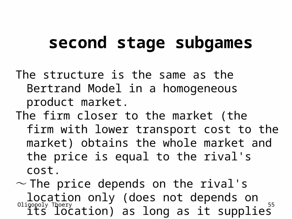
second stage subgames
The structure is the same as the Bertrand Model in a homogeneous product market.
The firm closer to the market (the firm with lower transport cost to the market) obtains the whole market and the price is equal to the rival's cost.
~ The price depends on the rival's location only (does not depends on its location) as long as it supplies for the market.
Oligopoly Thoery 56
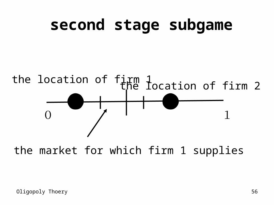
second stage subgame
0 1
the location of firm 1the location of firm 2
the market for which firm 1 supplies
Oligopoly Thoery 57
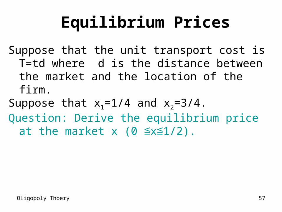
Equilibrium Prices
Suppose that the unit transport cost is T=td where d is the distance between the market and the location of the firm.
Suppose that x1=1/4 and x2=3/4.Question: Derive the equilibrium price at the market x
(0 x 1/2).≦ ≦
Oligopoly Thoery 58
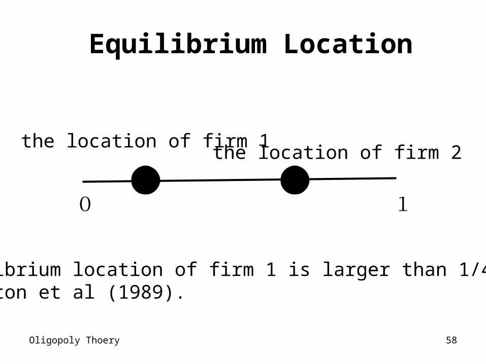
Equilibrium Location
0 1
the location of firm 1the location of firm 2
Equilibrium location of firm 1 is larger than 1/4Hamilton et al (1989).
Oligopoly Thoery 59
Equilibrium LocationFirm 1 chooses its location so as to minimize the
transport cost given the prices of the rival. If the demand is inelastic, firm 1 chooses 1/4 (central
point of its supply area). If the demand is elastic, firm 1 put a larger weight on
the market for which it supplies larger output. →Firm 1 chooses a location closer to the central point
1/2.
Oligopoly Thoery 60
Equilibrium LocationThe relocation affects the supply area. Should firm 1 consider this effect when it chooses its
location rather than considering transport cost only.→The profit from the marginal market is zero, so the
marginal expansion of the supply area does not affect the profits.
→Firms care about its transport costs only.
Oligopoly Thoery 61
Spatial Cournot ModelConsider a symmetric duopoly. Transport cost is proportional to both distance and
output quantity (linear transport cost). In the first stage, each firm chooses its location
independently.In the second stage, each firm chooses its output
independently.Each point has an independent market, and the
demand function is linear demand function, P=A-Y. No consumer's arbitrage. Production cost is normalized as zero. A is sufficiently large.
Hamilton et al (1989), Anderson and Neven (1991)
Oligopoly Thoery 62
Properties of Spatial Cournot Model
Market overlap ~ Two firms supply for all markets
Market share depends on the locations of the two firms.
Oligopoly Thoery 63
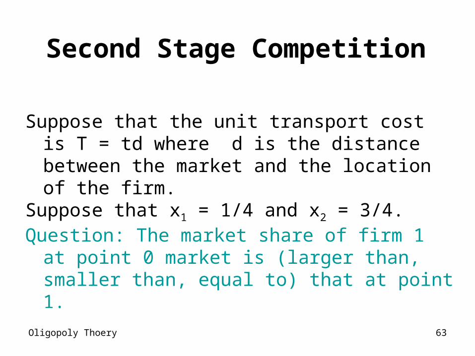
Second Stage Competition
Suppose that the unit transport cost is T = td where d is the distance between the market and the location of the firm.
Suppose that x1 = 1/4 and x2 = 3/4.Question: The market share of firm 1 at point 0
market is (larger than, smaller than, equal to) that at point 1.
Oligopoly Thoery 64
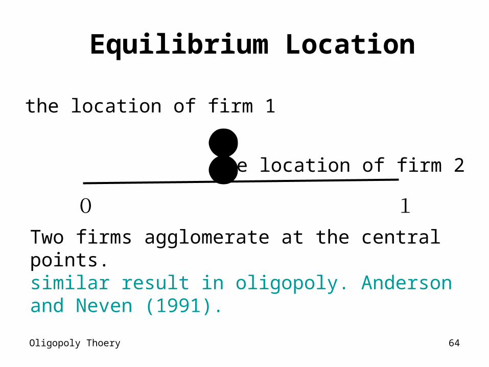
Equilibrium Location
0 1
the location of firm 1
the location of firm 2
Two firms agglomerate at the central points.similar result in oligopoly. Anderson and Neven (1991).
Oligopoly Thoery 65
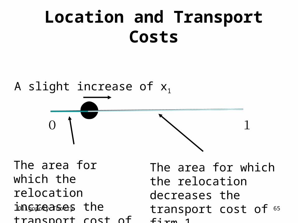
Location and Transport Costs
0 1
A slight increase of x1
The area for which the relocation increases the transport cost of firm 1
The area for which the relocation decreases the transport cost of firm 1
Oligopoly Thoery 66
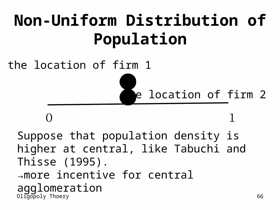
Non-Uniform Distribution of Population
0 1
the location of firm 1
the location of firm 2
Suppose that population density is higher at central, like Tabuchi and Thisse (1995).→more incentive for central agglomeration
Oligopoly Thoery 67
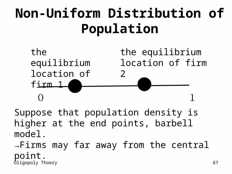
Non-Uniform Distribution of Population
0 1
the equilibrium location of firm 1
the equilibrium location of firm 2
Suppose that population density is higher at the end points, barbell model.→Firms may far away from the central point.
Oligopoly Thoery 68
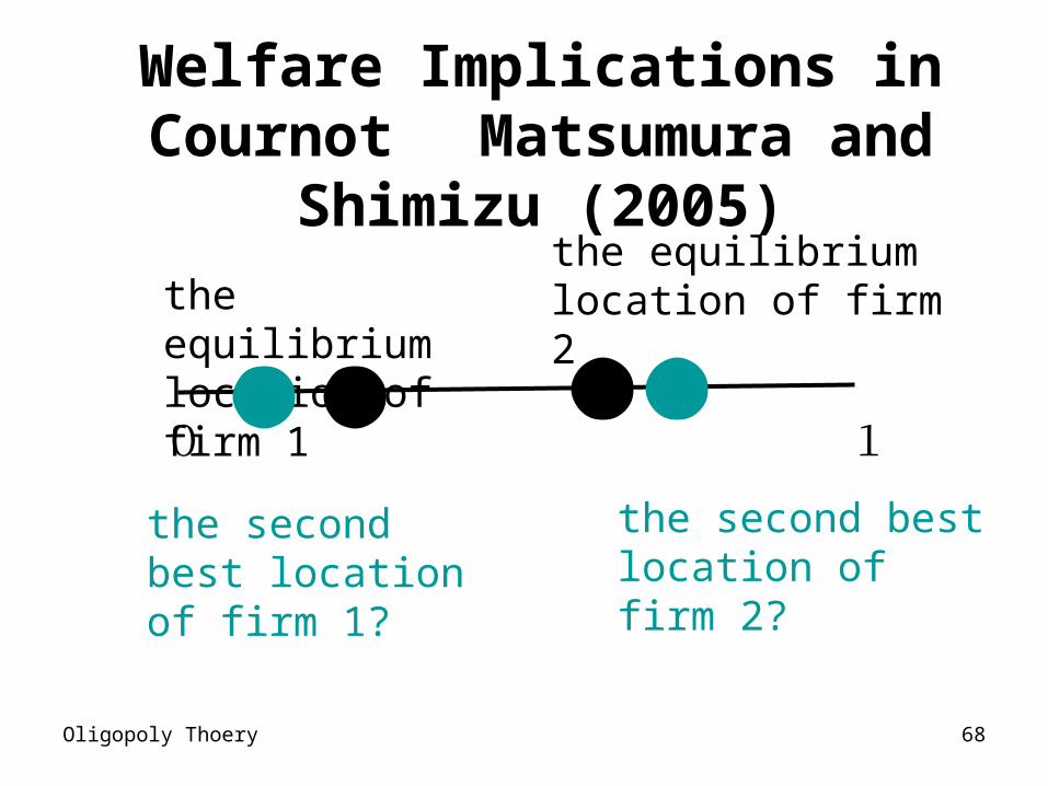
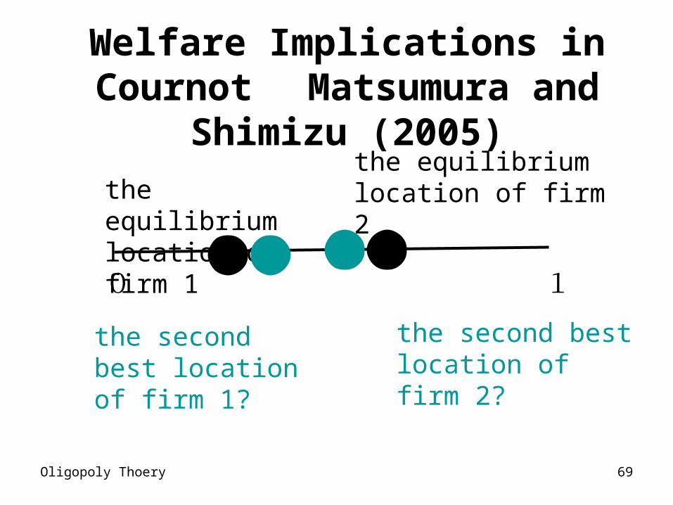
Welfare Implications in Cournot Matsumura and Shimizu (2005)
0 1
the equilibrium location of firm 1
the equilibrium location of firm 2
the second best location of firm 1?
the second best location of firm 2?
Oligopoly Thoery 69
Welfare Implications in Cournot Matsumura and Shimizu (2005)
0 1
the equilibrium location of firm 1
the equilibrium location of firm 2
the second best location of firm 1?
the second best location of firm 2?
Oligopoly Thoery 70
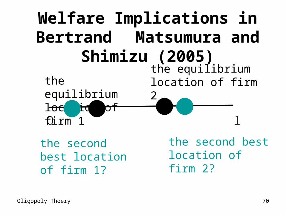
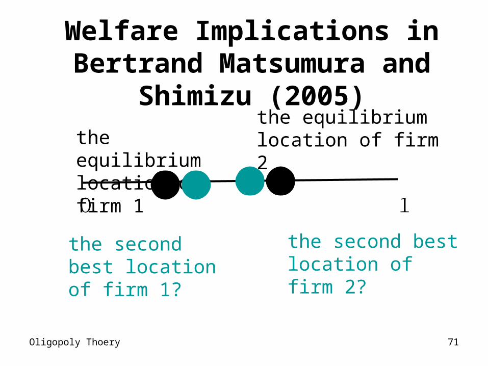
Welfare Implications in Bertrand Matsumura and Shimizu (2005)
0 1
the equilibrium location of firm 1
the equilibrium location of firm 2
the second best location of firm 1?
the second best location of firm 2?
Oligopoly Thoery 71
Welfare Implications in Bertrand Matsumura and Shimizu (2005)
0 1
the equilibrium location of firm 1
the equilibrium location of firm 2
the second best location of firm 1?
the second best location of firm 2?
Oligopoly Thoery 72
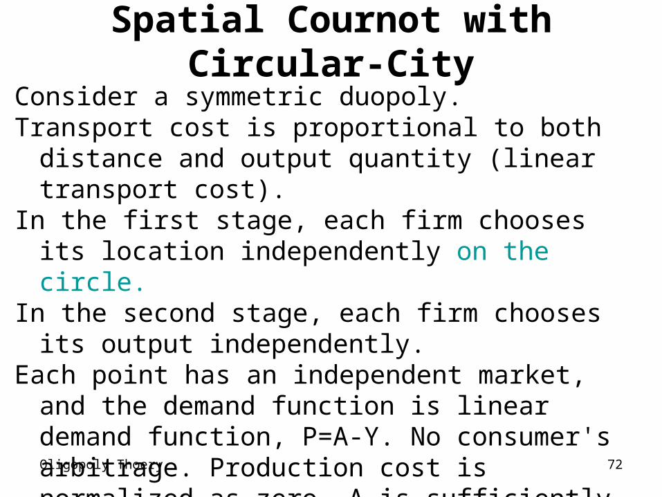
Spatial Cournot with Circular-CityConsider a symmetric duopoly. Transport cost is proportional to both distance and
output quantity (linear transport cost). In the first stage, each firm chooses its location
independently on the circle.In the second stage, each firm chooses its output
independently.Each point has an independent market, and the
demand function is linear demand function, P=A-Y. No consumer's arbitrage. Production cost is normalized as zero. A is sufficiently large.
Pal (1998)
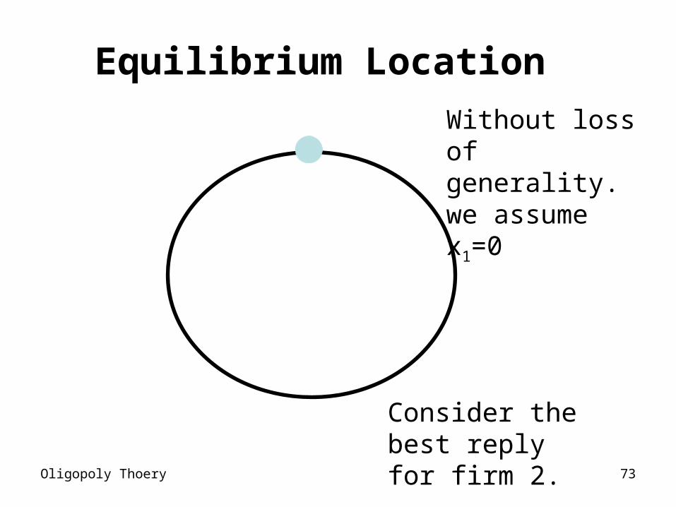
Oligopoly Thoery 73
Equilibrium Location Without loss of generality. we assume x1=0
Consider the best reply for firm 2.
Oligopoly Thoery74
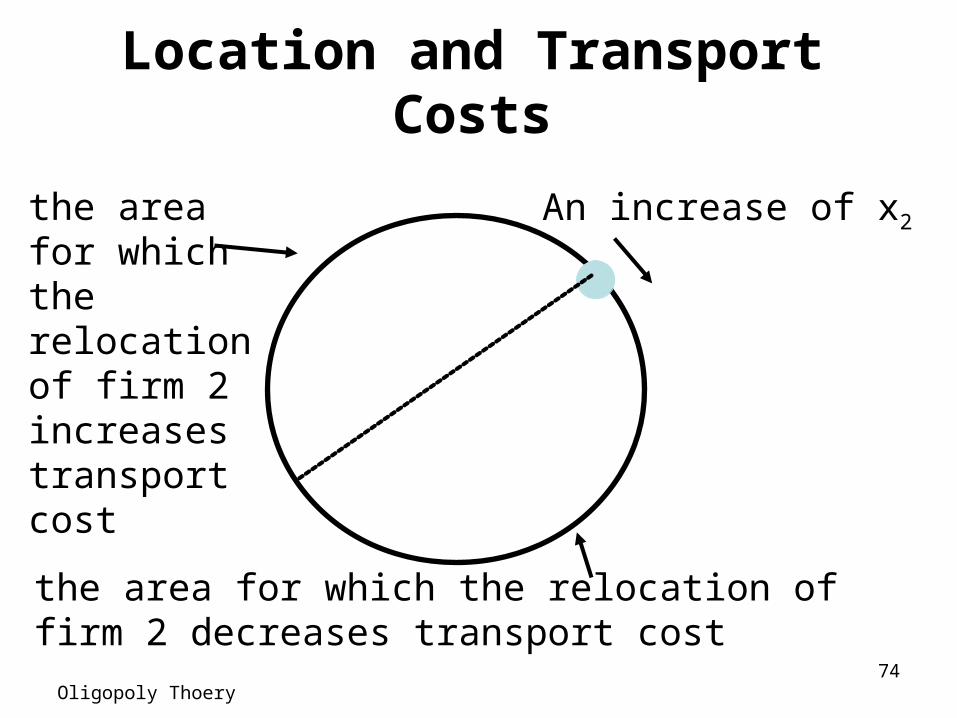
Location and Transport Costs
An increase of x2
the area for which the relocation of firm 2 decreases transport cost
the area for which the relocation of firm 2 increases transport cost
Oligopoly Thoery 75
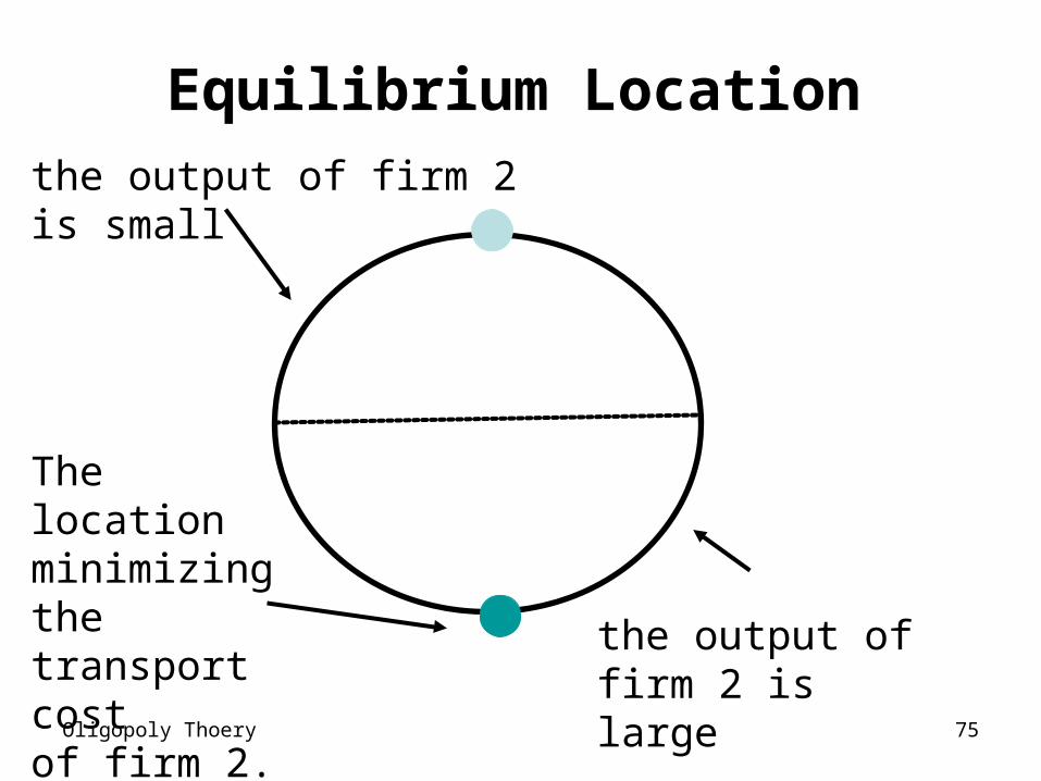
Equilibrium Location
the output of firm 2 is large
the output of firm 2 is small
The location minimizing the transport costof firm 2.
Oligopoly Thoery 76
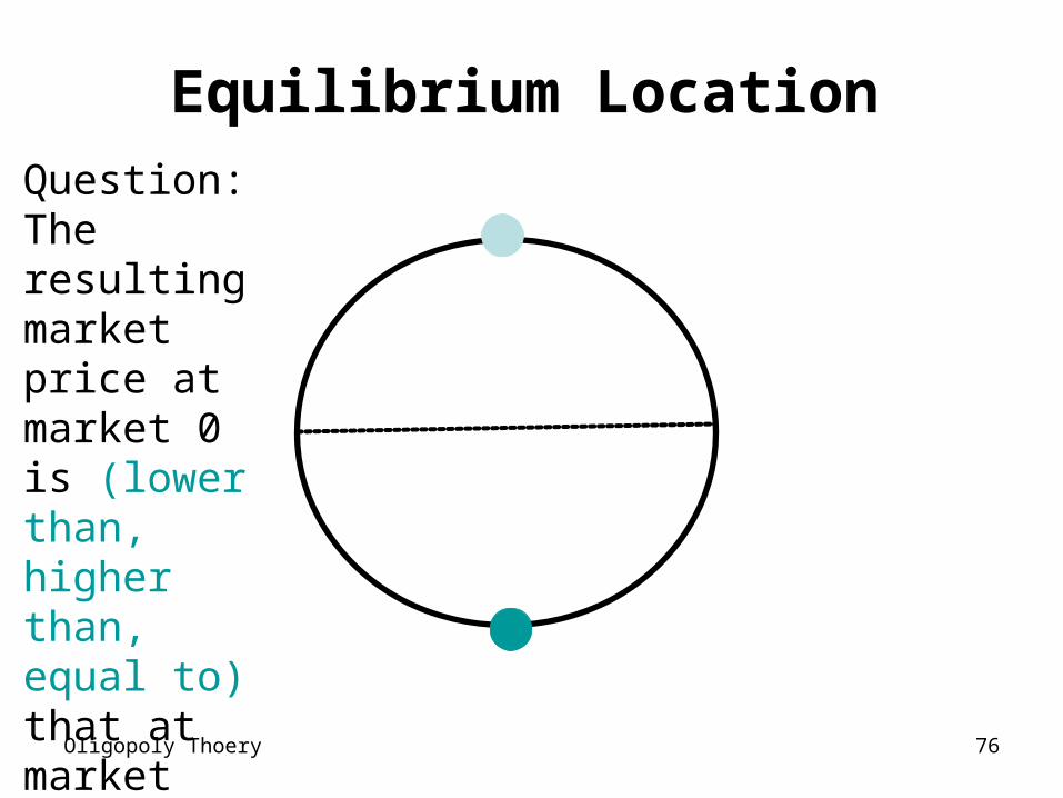
Equilibrium LocationQuestion:The resulting market price at market 0 is (lower than, higher than, equal to) that at market 1/4.
Oligopoly Thoery 77
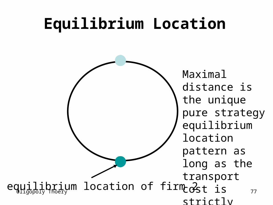
Equilibrium Location
the equilibrium location of firm 2
Maximal distance is the unique pure strategy equilibrium location pattern as long as the transport cost is strictly increasing.
Oligopoly Thoery 78
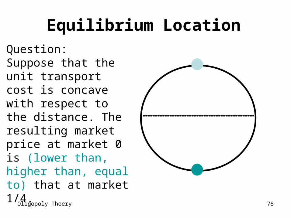
Equilibrium LocationQuestion:Suppose that the unit transport cost is concave with respect to the distance. The resulting market price at market 0 is (lower than, higher than, equal to) that at market 1/4.
Oligopoly Thoery 79
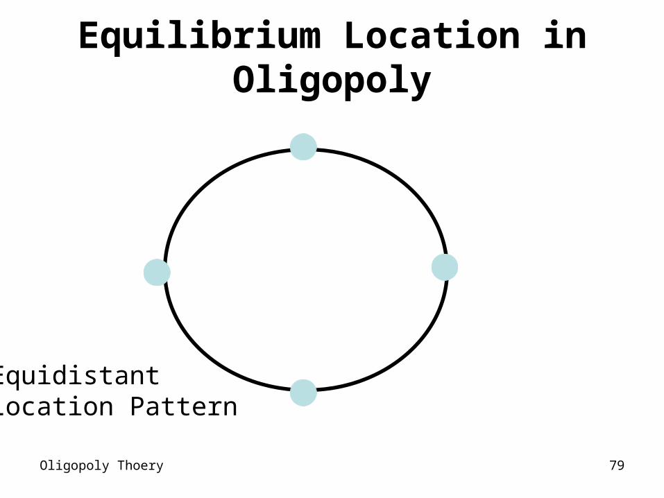
Equilibrium Location in Oligopoly
Equidistant Location Pattern
Oligopoly Thoery 80
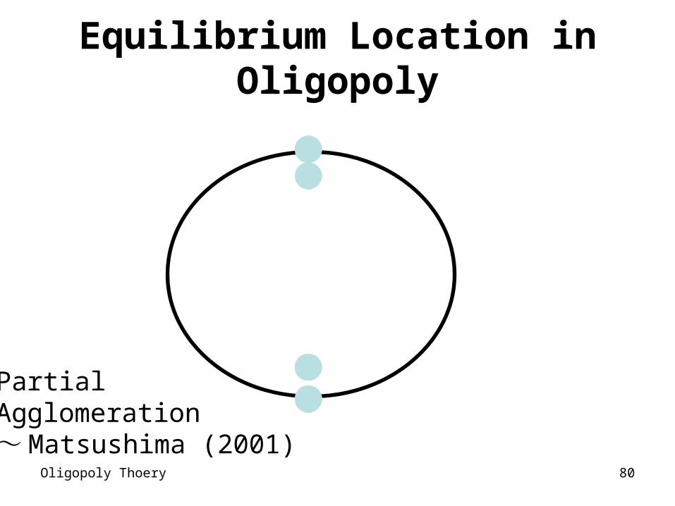
Equilibrium Location in Oligopoly
Partial Agglomeration~ Matsushima (2001)
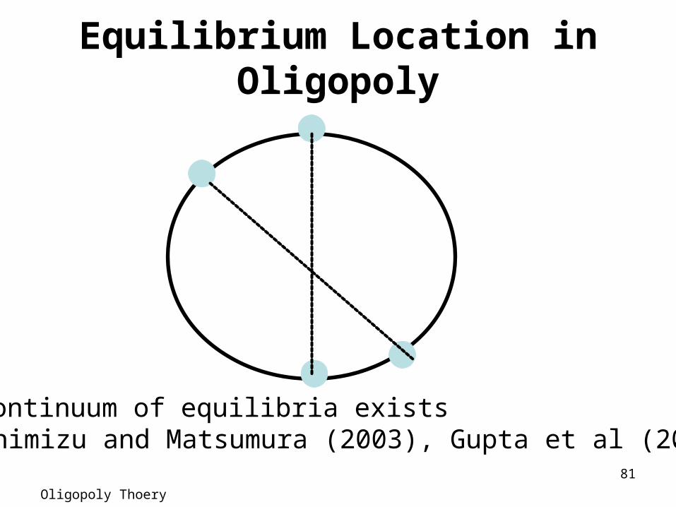
Oligopoly Thoery
81
Equilibrium Location in Oligopoly
a continuum of equilibria exists~ Shimizu and Matsumura (2003), Gupta et al (2004)
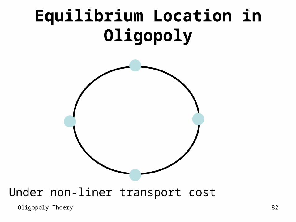
Oligopoly Thoery 82
Equilibrium Location in Oligopoly
Under non-liner transport cost
Oligopoly Thoery 83
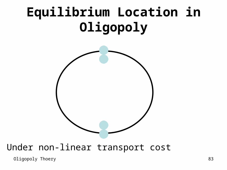
Equilibrium Location in Oligopoly
Under non-linear transport cost
Oligopoly Thoery 84
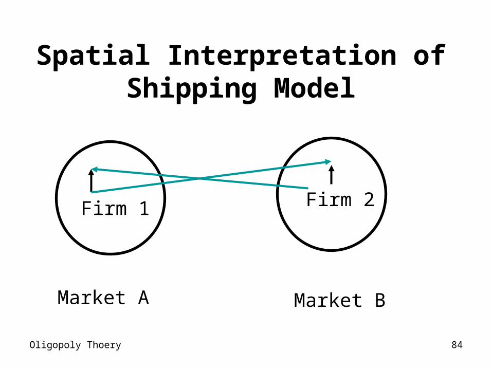
Spatial Interpretation of Shipping Model
Market A
Firm 1 Firm 2
Market B
Oligopoly Thoery 85
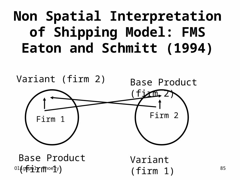
Non Spatial Interpretation of Shipping Model: FMS Eaton and
Schmitt (1994)
Base Product (firm 1)
Firm 1 Firm 2
Variant (firm 1)
Variant (firm 2) Base Product (firm 2)

Oligopoly Thoery 86
Non Spatial Interpretation of Shipping Model: Technological
Choice (Matsumura (2004))
Market A:
Small Car
Firm 1 Firm 2
Market B:
Large Car
Oligopoly Thoery 87
Mixed Strategy Equilibria
Oligopoly Thoery 88
Uniqueness of the EquilibriumShopping, Hotelling, quadratic transport cost, uniform
distribution ( standard Location-Price Model)The unique pure strategy equilibrium location pattern
is maximal differentiation.However, there are two pure strategy equilibria. (x1, x2)=(0,1), (x1, x2)=(1,0) →Mixed strategy equilibria may exist. In fact, many (infinite) mixed strategy equilibria exist
Bester et al (1996).
Oligopoly Thoery 89
Cost Differential between Firms
Consider a production cost difference between two firms.
When the cost difference between two firms is small, the maximal differentiation is the unique pure strategy equilibrium location pattern.
When the cost difference between two firms is large, no pure strategy equilibrium exists.
Suppose that firm 1 is a lower cost firm and the cost difference is large. The best location of firm 1 is x1=x2 (minimal differentiation), while that of firm 2 is either x2=1 or x2=0 (maximal differentiation).

Oligopoly Thoery 90
Cost Differential between Firms
Consider a production cost difference between two firms.
When the cost difference between two firms is large, no pure strategy equilibrium exists.
In this case, the following constitutes a mixed strategy equilibrium.
Both firms choose two edges with probability 1/2.This does not constitute a mixed strategy equilibria
without cost difference.
Oligopoly Thoery 91
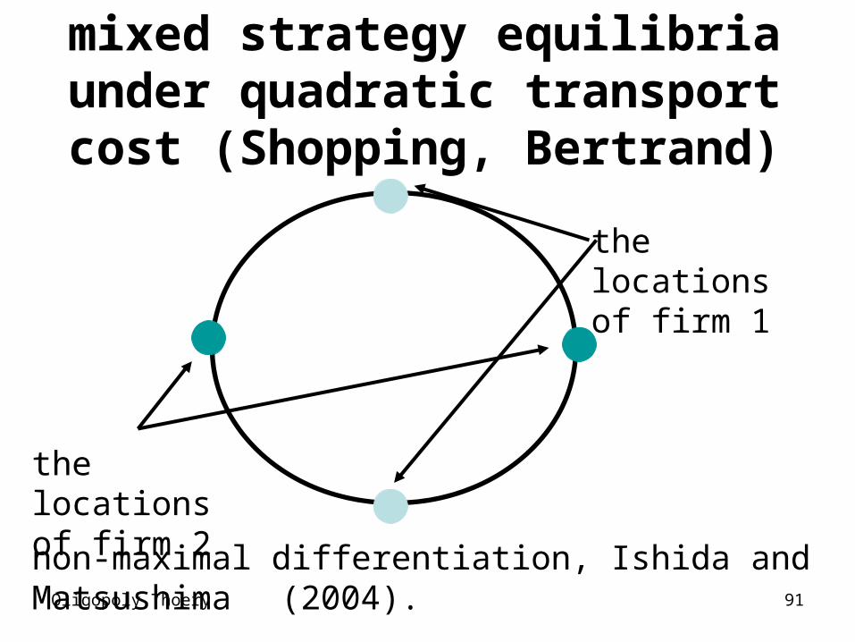
mixed strategy equilibria under quadratic transport cost (Shopping,
Bertrand)
the locations of firm 1
the locations of firm 2
non-maximal differentiation, Ishida and Matsushima (2004).
Oligopoly Thoery 92
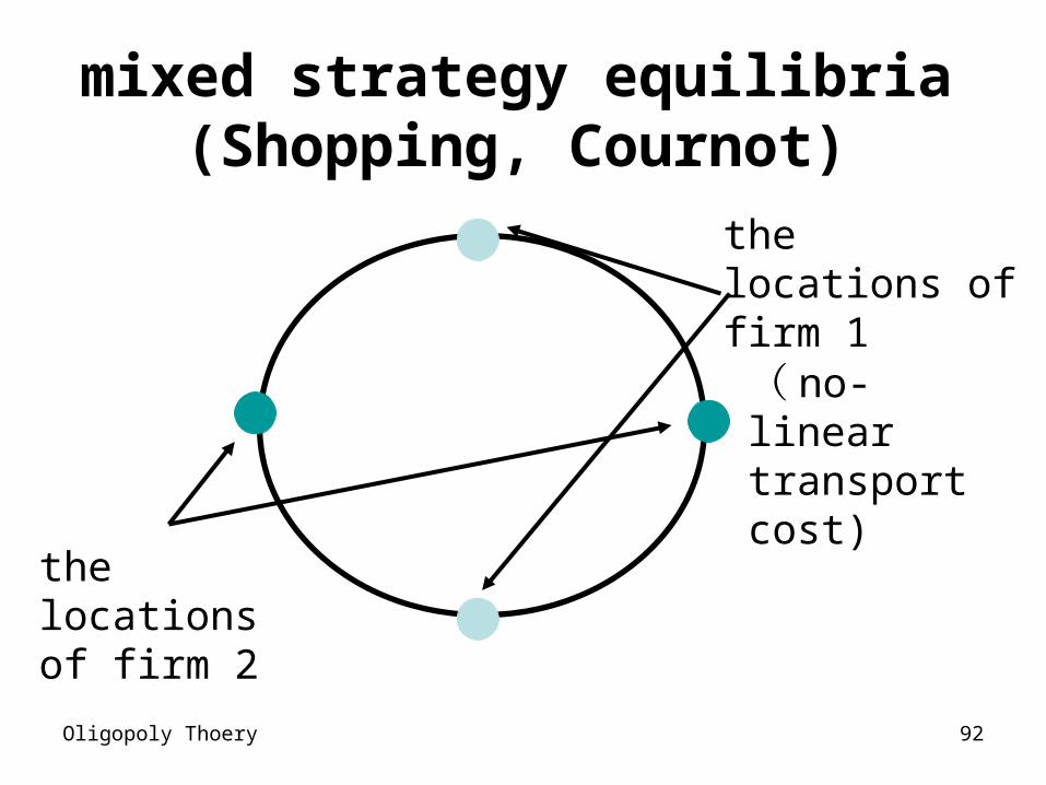
mixed strategy equilibria (Shopping, Cournot)
the locations of firm 1
the locations of firm 2
( no-linear transport cost)
Oligopoly Thoery 93
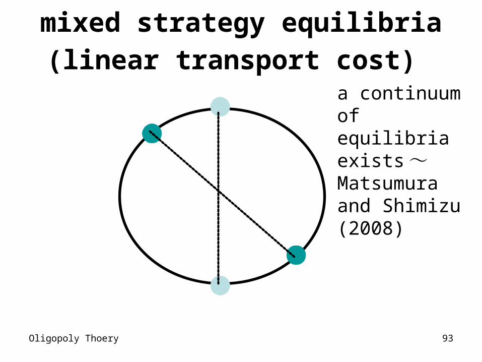
mixed strategy equilibria (linear
transport cost) a continuum of equilibria exists~ Matsumura and Shimizu (2008)
Oligopoly Thoery 94
Two Standard Models of Space
(1) Hotelling type Linear-City Model
(2) Salop type (or Vickery type) Circular-City Model
Linear-City has a center-periphery structure, while every point in the Circular-City is identical.
→Circular Model is more convenient than Linear Model for discussing symmetric oligopoly except for duopoly.
Oligopoly Thoery 95
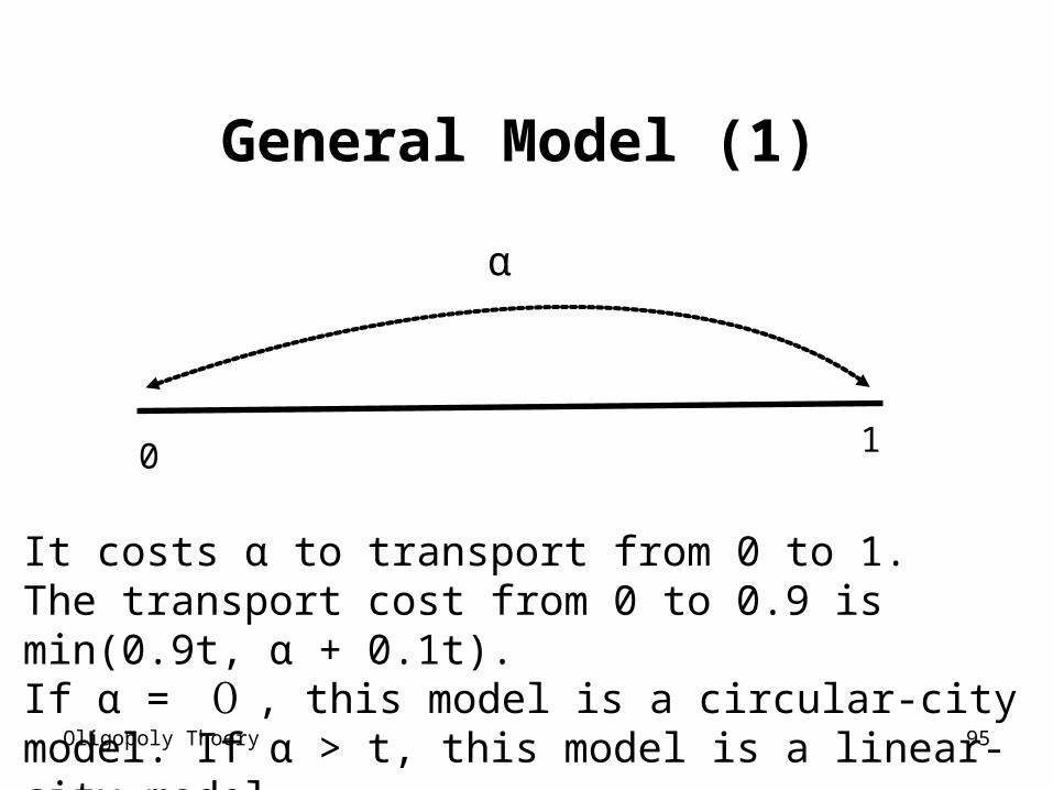
General Model (1)
0 1
α
It costs α to transport from 0 to 1. The transport cost from 0 to 0.9 is min(0.9t, α + 0.1t).If α = 0 , this model is a circular-city model. If α > t, this model is a linear-city model.
Oligopoly Thoery 96
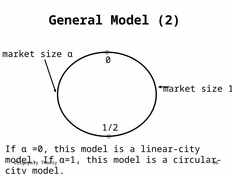
General Model (2)
0
1/2
market size 1
market size α
If α =0, this model is a linear-city model. If α=1, this model is a circular-city model.
Oligopoly Thoery 97
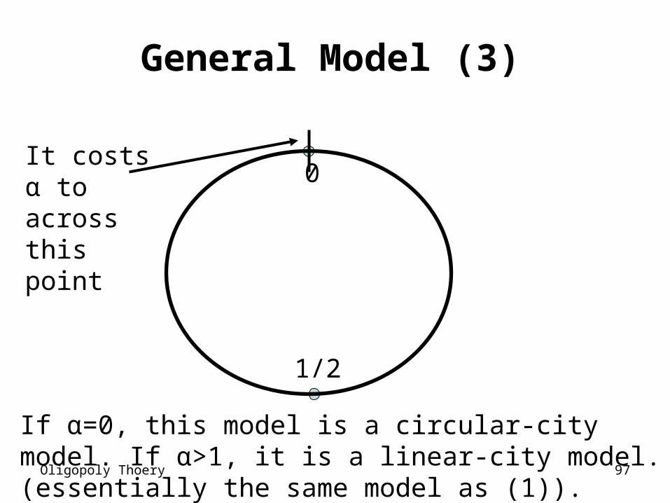
General Model (3)
0
1/2
It costs α to across this point
If α=0, this model is a circular-city model. If α>1, it is a linear-city model. (essentially the same model as (1)).
Oligopoly Thoery 98
ApplicationIn the mill pricing (shopping) location-price models,
both linear-city and circular-city models yield maximal differentiation.
delivered pricing model (shipping model) →linear-city model and circular-city model yield different location patterns~ We discuss this shipping model.
Oligopoly Thoery 99
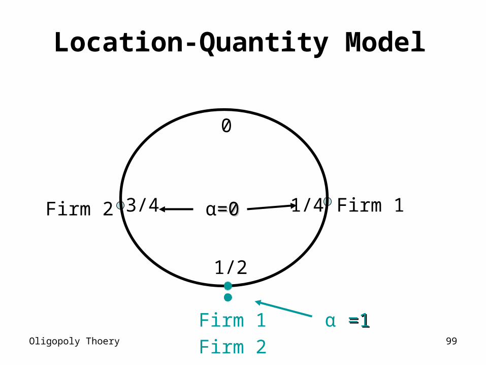
Location-Quantity Model
0
1/2
Firm 1Firm 2
Firm 1
Firm 2
α =1 =1
α=0=0 1/43/4
Oligopoly Thoery 100
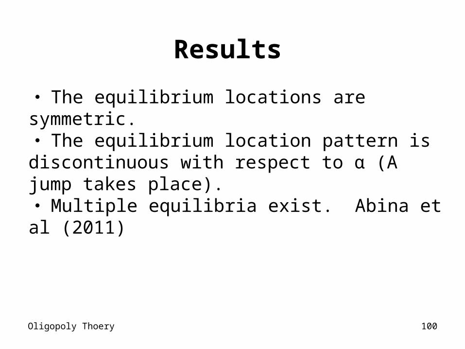
Results
・ The equilibrium locations are symmetric.・ The equilibrium location pattern is discontinuous with respect to α (A jump takes place). ・ Multiple equilibria exist. Abina et al (2011)
Oligopoly Thoery 101
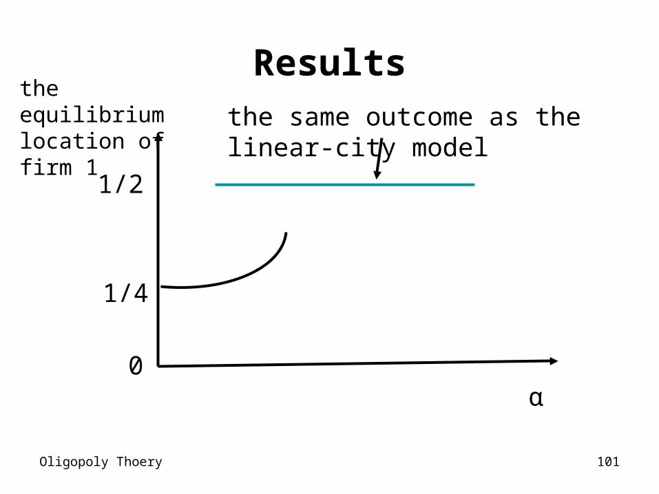
Resultsthe equilibrium location of firm 1
α0
1/2
1/4
the same outcome as the linear-city model
Oligopoly Thoery 102
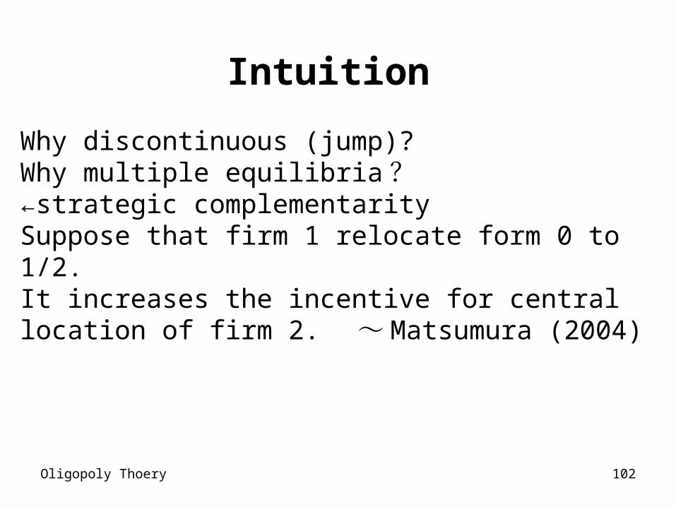
Intuition
Why discontinuous (jump)?Why multiple equilibria ?←strategic complementaritySuppose that firm 1 relocate form 0 to 1/2. It increases the incentive for central location of firm 2. ~ Matsumura (2004)
Oligopoly Thoery 103
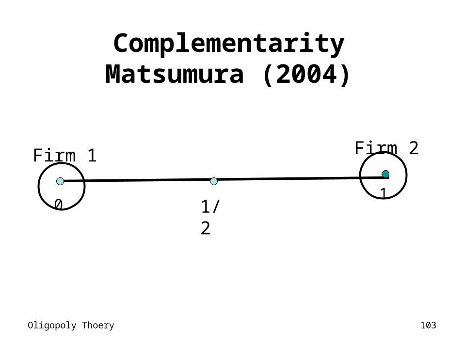
ComplementarityMatsumura (2004)
01
1/2
Firm 1 Firm 2
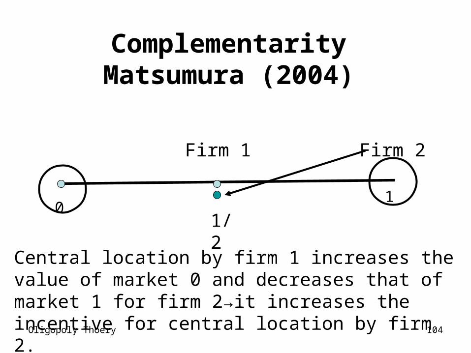
Oligopoly Thoery 104
ComplementarityMatsumura (2004)
01
1/2
Firm 2Firm 1
Central location by firm 1 increases the value of market 0 and decreases that of market 1 for firm 2→it increases the incentive for central location by firm 2.
Oligopoly Theory 105
Shopping or ShippingFirms may be able to choose their pricing strategies. Shopping → Uniform pricing, FOB pricing: the price
does not depends on the location or personal properties.
Shipping → Spatial price discrimination, CIF pricing: the prices depend on the location or personal properties.
Thisse and Vives (1988) endogenize this choice. (1)Both firms choose delivered pricing (personal
pricing)(2)Uniform pricing is mutually beneficial for firms
(prisoners’ dilemma)