omnichannel operations management
TRANSCRIPT

University of Pennsylvania University of Pennsylvania
ScholarlyCommons ScholarlyCommons
Publicly Accessible Penn Dissertations
2017
Omnichannel Operations Management Omnichannel Operations Management
Fei Gao University of Pennsylvania, [email protected]
Follow this and additional works at: https://repository.upenn.edu/edissertations
Recommended Citation Recommended Citation Gao, Fei, "Omnichannel Operations Management" (2017). Publicly Accessible Penn Dissertations. 2296. https://repository.upenn.edu/edissertations/2296
This paper is posted at ScholarlyCommons. https://repository.upenn.edu/edissertations/2296 For more information, please contact [email protected].
Omnichannel Operations Management Omnichannel Operations Management
Abstract Abstract This dissertation studies how a firm could effectively make use of different selling channels to provide consumers with a seamless shopping experience. In the three essays, by analyzing stylized models where firms operates both online and offline channels and consumers strategically make channel choices, we examine the impacts of different types of omnichannel strategies in different industries. In the first essay, we focus on a specific omnichannel fulfillment strategy, i.e., buy-online-and-pick-up-in-store (BOPS). We find it may not be profitable to implement BOPS on products that sell well in stores. We also consider a decentralized retail system where store and online channels are managed separately, and find it is rarely efficient to allocate all BOPS revenue to a single channel. In the second essay, we study how retailers can effectively deliver product and inventory information to omnichannel consumers who strategically choose whether to gather information online/offline and whether to buy products online/offline. Specifically, we consider three information mechanisms: physical showrooms, virtual showrooms, and availability information. Our main result is that these information mechanisms may sometimes change customers’ channel choice in a way such that total product returns increase and total retail profit decreases. In the third essay, we look at the restaurant industry. Specifically, we study the impacts of different self-order technologies on service operations. Online technology, through websites and mobile apps, allows customers to order and pay before coming to the store; offline technology, such as self-service kiosks, allows store customers to place orders without interacting with a human employee. We develop a stylized queueing model and study the impacts of self-order technologies on customer demand, employment levels, and restaurant profits. We find there could be a win-win-win situation, where everyone in the market, i.e., consumers (including those who do not use the technology), workers and the firm, could benefit from the implementation of the self-order technologies.
Degree Type Degree Type Dissertation
Degree Name Degree Name Doctor of Philosophy (PhD)
Graduate Group Graduate Group Operations & Information Management
First Advisor First Advisor Xuanming Su
Keywords Keywords Consumer Behavior, Market-Operations Interface, Omnichannel, Operations Management
This dissertation is available at ScholarlyCommons: https://repository.upenn.edu/edissertations/2296
OMNICHANNEL OPERATIONS MANAGEMENT
Fei Gao
A DISSERTATION
in
Operations, Information and Decisions
For the Graduate Group in Managerial Science and Applied Economics
Presented to the Faculties of the University of Pennsylvania
in
Partial Fulfillment of the Requirements for the
Degree of Doctor of Philosophy
2017
Supervisor of Dissertation
Xuanming Su, Murrel J. Ades Professor of Operations, Information and Decisions
Graduate Group Chairperson
Catherine Schrand, Celia Z. Moh Professor, Professor of Accounting
Dissertation Committee
Gerard P. Cachon, Fred R. Sullivan Professor of Operations, Information, and Decisions
Morris A. Cohen, Panasonic Professor of Manufacturing & Logistics, Professor ofOperations, Information and Decisions
OMNICHANNEL OPERATIONS MANAGEMENT
c© COPYRIGHT
2017
Fei Gao
This work is licensed under the
Creative Commons Attribution
NonCommercial-ShareAlike 3.0
License
To view a copy of this license, visit
http://creativecommons.org/licenses/by-nc-sa/3.0/

ACKNOWLEDGEMENT
First and foremost, I would like to express my sincere gratitude to my advisor, Professor
Xuanming Su, for his guidance and support. I am truly fortunate to work with him. His
guidance helped me in all the time of research and writing of this thesis. I could not have
imagined having a better advisor and mentor for my PhD study.
I am also extremely grateful to Professors Gerard Cachon and Morris Cohen, who are also on
my dissertation committee, for their detailed and insightful comments on my dissertation.
Moreover, I really appreciate their generous support and advice during my job market
process.
Finally, and most importantly, I would like to thank my parents, Hong Liang and Jianshe
Gao, for their support, encouragement and unwavering love throughout my life.
iii
ABSTRACT
OMNICHANNEL OPERATIONS MANAGEMENT
Fei Gao
Xuanming Su
This dissertation studies how a firm could effectively make use of different selling channels
to provide consumers with a seamless shopping experience. In the three essays, by analyz-
ing stylized models where firms operates both online and offline channels and consumers
strategically make channel choices, we examine the impacts of different types of omnichan-
nel strategies in different industries. In the first essay, we focus on a specific omnichannel
fulfillment strategy, i.e., buy-online-and-pick-up-in-store (BOPS). We find it may not be
profitable to implement BOPS on products that sell well in stores. We also consider a de-
centralized retail system where store and online channels are managed separately, and find
it is rarely efficient to allocate all BOPS revenue to a single channel. In the second essay,
we study how retailers can effectively deliver product and inventory information to om-
nichannel consumers who strategically choose whether to gather information online/offline
and whether to buy products online/offline. Specifically, we consider three information
mechanisms: physical showrooms, virtual showrooms, and availability information. Our
main result is that these information mechanisms may sometimes change customers chan-
nel choice in a way such that total product returns increase and total retail profit decreases.
In the third essay, we look at the restaurant industry. Specifically, we study the impacts of
different self-order technologies on service operations. Online technology, through websites
and mobile apps, allows customers to order and pay before coming to the store; offline tech-
nology, such as self-service kiosks, allows store customers to place orders without interacting
with a human employee. We develop a stylized queueing model and study the impacts of
self-order technologies on customer demand, employment levels, and restaurant profits. We
find there could be a win-win-win situation, where everyone in the market, i.e., consumers
iv
(including those who do not use the technology), workers and the firm, could benefit from
the implementation of the self-order technologies.
v
TABLE OF CONTENTS
ACKNOWLEDGEMENT . . . . . . . . . . . . . . . . . . . . . . . . . . . . . . . . . iii
ABSTRACT . . . . . . . . . . . . . . . . . . . . . . . . . . . . . . . . . . . . . . . . iv
LIST OF ILLUSTRATIONS . . . . . . . . . . . . . . . . . . . . . . . . . . . . . . . viii
CHAPTER 1 : Introduction . . . . . . . . . . . . . . . . . . . . . . . . . . . . . . . 1
CHAPTER 2 : Omnichannel Retail Operations with Buy-Online-and-Pick-up-in-Store 3
2.1 Introduction . . . . . . . . . . . . . . . . . . . . . . . . . . . . . . . . . . . . 3
2.2 Literature Review . . . . . . . . . . . . . . . . . . . . . . . . . . . . . . . . 6
2.3 Model . . . . . . . . . . . . . . . . . . . . . . . . . . . . . . . . . . . . . . . 9
2.4 Information Effect and Convenience Effect . . . . . . . . . . . . . . . . . . . 15
2.5 Heterogeneous Customers . . . . . . . . . . . . . . . . . . . . . . . . . . . . 22
2.6 Decentralized System . . . . . . . . . . . . . . . . . . . . . . . . . . . . . . . 27
2.7 Conclusion . . . . . . . . . . . . . . . . . . . . . . . . . . . . . . . . . . . . 31
CHAPTER 3 : Online and Offline Information for Omnichannel Retailing . . . . . 34
3.1 Introduction . . . . . . . . . . . . . . . . . . . . . . . . . . . . . . . . . . . . 34
3.2 Literature Review . . . . . . . . . . . . . . . . . . . . . . . . . . . . . . . . 38
3.3 Base Model . . . . . . . . . . . . . . . . . . . . . . . . . . . . . . . . . . . . 40
3.4 Physical Showrooms . . . . . . . . . . . . . . . . . . . . . . . . . . . . . . . 44
3.5 Virtual Showrooms . . . . . . . . . . . . . . . . . . . . . . . . . . . . . . . . 48
3.6 Availability Information . . . . . . . . . . . . . . . . . . . . . . . . . . . . . 51
3.7 Joint Implementation . . . . . . . . . . . . . . . . . . . . . . . . . . . . . . 54
3.8 Extensions . . . . . . . . . . . . . . . . . . . . . . . . . . . . . . . . . . . . . 59
3.9 Conclusion . . . . . . . . . . . . . . . . . . . . . . . . . . . . . . . . . . . . 62
vi
CHAPTER 4 : Omnichannel Service Operations with Online and Offline Self-Order
Technologies . . . . . . . . . . . . . . . . . . . . . . . . . . . . . . . 64
4.1 Introduction . . . . . . . . . . . . . . . . . . . . . . . . . . . . . . . . . . . . 64
4.2 Literature Review . . . . . . . . . . . . . . . . . . . . . . . . . . . . . . . . 68
4.3 Base Model . . . . . . . . . . . . . . . . . . . . . . . . . . . . . . . . . . . . 71
4.4 Online Self-Order Technology . . . . . . . . . . . . . . . . . . . . . . . . . . 72
4.5 Offline Self-Order Technology . . . . . . . . . . . . . . . . . . . . . . . . . . 80
4.6 Profit Implications . . . . . . . . . . . . . . . . . . . . . . . . . . . . . . . . 86
4.7 Extensions . . . . . . . . . . . . . . . . . . . . . . . . . . . . . . . . . . . . . 90
4.8 Conclusion . . . . . . . . . . . . . . . . . . . . . . . . . . . . . . . . . . . . 92
APPENDIX . . . . . . . . . . . . . . . . . . . . . . . . . . . . . . . . . . . . . . . . . 95
A.1 Decentralized System in Heterogeneous Market . . . . . . . . . . . . . . . . 95
A.2 Model Extensions to Chapter 2 . . . . . . . . . . . . . . . . . . . . . . . . . 96
A.3 Detailed Analyses of Scenarios When Multiple Mechanisms are Provided Si-
multaneously . . . . . . . . . . . . . . . . . . . . . . . . . . . . . . . . . . . 105
A.4 Model Extensions to Chapter 3 . . . . . . . . . . . . . . . . . . . . . . . . . 108
A.5 Numerical Study for Chapter 3 . . . . . . . . . . . . . . . . . . . . . . . . . 127
A.6 Model Extensions to Chapter 4 . . . . . . . . . . . . . . . . . . . . . . . . . 129
A.7 Proofs . . . . . . . . . . . . . . . . . . . . . . . . . . . . . . . . . . . . . . . 142
BIBLIOGRAPHY . . . . . . . . . . . . . . . . . . . . . . . . . . . . . . . . . . . . . 229
vii
LIST OF ILLUSTRATIONS
FIGURE 1 : Do consumers buy the product in store? . . . . . . . . . . . . . . 16
FIGURE 2 : Impacts of BOPS hassle cost hb and cross-selling benefit r . . . . 20
FIGURE 3 : Market Segmentation with and without BOPS . . . . . . . . . . . 25
FIGURE 4 : When do consumers go to store? . . . . . . . . . . . . . . . . . . . 26
FIGURE 5 : Comparison of consumer behavior with and without physical show-
room . . . . . . . . . . . . . . . . . . . . . . . . . . . . . . . . . . 47
FIGURE 6 : Comparison of consumer behavior with and without virtual showroom 50
FIGURE 7 : Comparison of consumer behavior with and without availability
information . . . . . . . . . . . . . . . . . . . . . . . . . . . . . . . 53
FIGURE 8 : Impact of Online Self-Order Technology on Workforce Level . . . 79
FIGURE 9 : Do consumers buy the product in store? . . . . . . . . . . . . . . 98
FIGURE 10 : Do strategic consumers buy the product in store? . . . . . . . . . 103
FIGURE 11 : Proportion of instances that physical showrooms backfire (i.e., πo >
πp) . . . . . . . . . . . . . . . . . . . . . . . . . . . . . . . . . . . 129
FIGURE 12 : Proportion of instances that virtual showrooms backfire (i.e., πo >
πv) . . . . . . . . . . . . . . . . . . . . . . . . . . . . . . . . . . . 130
FIGURE 13 : Proportion of instances that total workforce level increases after the
implementation of online self-order technology (i.e., ko1 +ko2 > kb1 +kb2)141
FIGURE 14 : Proportion of instances that total workforce level increases after the
implementation of offline self-order technology (i.e., ks1 +ks2 > kb1 +kb2)142
FIGURE 15 : Proportion of instances that online self-order technology generates
more profit than offline self-order technology (i.e., πo > πs) . . . . 142
viii
CHAPTER 1 : Introduction
The general topic of this dissertation is omnichannel operations management. Nowadays,
firms have many different channels to reach their customers. Instead of treating different
channels as independent silos, more and more firms realize the need to integrate different
channels to provide customers with a seamless shopping experience. This dissertation stud-
ies the impacts of various omnichannel strategies on consumer behavior and firm operational
efficiency through three essays.
In the first essay, we look at a specific omnichannel fulfillment strategy in the retail industry.
Many retailers have recently started to offer customers the option to buy online and pick
up in store (BOPS). We study the impact of the BOPS initiative on store operations. We
build a stylized model where a retailer operates both online and offline channels. Consumers
strategically make channel choices. The BOPS option affects consumer choice in two ways:
by providing real-time information about inventory availability and by reducing the hassle
cost of shopping. We obtain three findings. First, not all products are well-suited for in-
store pickup; specifically, it may not be profitable to implement BOPS on products that
sell well in stores. Second, BOPS enables retailers to reach new customers, but for existing
customers, the shift from online fulfillment to store fulfillment may decrease profit margins
when the latter is less cost effective. Finally, in a decentralized retail system where store
and online channels are managed separately, BOPS revenue can be shared across channels
to alleviate incentive conflicts; it is rarely efficient to allocate all the revenue to a single
channel.
In the second essay, we study how retailers can effectively deliver online and offline infor-
mation to omnichannel consumers who strategically choose whether to gather information
online/offline and whether to buy products online/offline. Information resolves two types of
uncertainty: product value uncertainty (i.e., consumers realize valuations when they inspect
the product in store, but may end up returning the product when they purchase online)
1
and availability uncertainty (i.e., store visits are futile when consumers encounter stock-
outs). We consider three information mechanisms: physical showrooms allow consumers to
learn valuations anytime they visit the store, even during stockouts; virtual showrooms give
consumers online access to an imperfect signal of their valuations; availability information
provides real-time information about whether the store is in stock. Our main results follow.
First, physical showrooms may prompt retailers to reduce store inventory, which increases
availability risk and discourages store patronage. Second, virtual showrooms may increase
online returns and hurt profits, if they induce excessive customer migration from store to
online channels. Third, availability information may be redundant when availability risk
is low, and may render physical showrooms ineffective when implemented jointly. Finally,
when customers are homogeneous, these mechanisms may not exhibit significant comple-
mentarities and the optimal information structure may involve choosing only one of the
three.
In the third essay, we shift focus to restaurant industry. Many restaurants have recently im-
plemented self-order technologies across both online and offline channels. Online technology,
through websites and mobile apps, allows customers to order and pay before coming to the
store; offline technology, such as self-service kiosks, allows store customers to place orders
without interacting with a human employee. In this essay, we develop a stylized theoreti-
cal model to study the impact of self-order technologies on customer demand, employment
levels, and restaurant profits. Our main results follow. First, customers using self- order
technologies experience reduced waiting cost and increased demand, and moreover, these
benefits may even carry over to customers who do not use these technologies. Second, al-
though public opinion suggests that self-order technologies facilitate job cuts, we find instead
that some firms should increase employment levels, and paradoxically, this recommendation
holds for firms with high labor costs. Finally, we find that firms should implement online
(offline) self-order technology when customers have high (low) wait sensitivity.
2
CHAPTER 2 : Omnichannel Retail Operations with
Buy-Online-and-Pick-up-in-Store
2.1. Introduction
As consumers become accustomed to online shopping, brick-and-mortar retailers have in-
creasingly supplemented their shops with online businesses (Financial Times, 2013). The
online channel has traditionally been viewed as a separate way to sell products. Today,
however, many retailers have realized the need to integrate their existing channels to en-
rich customer value proposition and improve operational efficiency. As a result, there is
an emerging focus on “omnichannel retailing” with the goal of providing consumers with
a seamless shopping experience through all available shopping channels (Bell et al., 2014;
Brynjolfsson et al., 2013; Rigby, 2011). When asked about omnichannel priorities, the re-
tailers surveyed by Forrester Research reported that fulfillment initiatives ranked higher
than any other channel integration program; moreover, among all omnichannel fulfillment
initiatives, allowing customers to buy online and pick up in store (BOPS) is regarded as the
most important one (Forrester, 2014). According to Retail Systems Research (RSR), as of
June 2013, 64% of retailers have implemented BOPS (RSR, 2013).
Retailers benefit from allowing customers to pick up their online orders in store. Specifi-
cally, BOPS generates store traffic and potentially increases sales (New York Times, 2011).
According to a recent UPS study, among those who have used an in-store pickup option,
45% of them have made a new purchase when picking up the purchase in store (UPS, 2015).
Typically, a substantial amount of store sales is generated through such cross-selling: it is
estimated that, on average, when a customer comes to the store intending to buy $100
worth of merchandise, they leave with $120 to $125 worth of merchandise (Washington
Post, 2015). Thus, unsurprisingly, more and more retailers are starting to offer the BOPS
functionality on their websites (RSR, 2013).
A key challenge facing retailers is to choose the right set of products for BOPS. Most
3
retailers generally agree that BOPS should not be a blanket functionality that is blindly
applied to all products across all categories. According to senior vice president and general
manager of Walmart.com, Steve Nave, one of the reasons for being selective is to focus on
those products that would “drive more customers into the stores” (Time, 2011). On the
websites of major retailers such as Toys R Us, customers will find that some products are not
eligible for BOPS. For example, new releases such as the LEGO Star Wars Sith Infiltrator
are not available for store pickup. These items are sold in stores, but shoppers need to check
their local stores for availability if they do not wish to wait for online delivery. In contrast,
for most of the extensive line of LEGO products sold on toysrus.com, the BOPS option is
available. Since retailers typically carry large numbers of SKUs online, a key challenge is
to understand the main criteria for selecting which product to allow for in-store pickup.
Many retailers regard BOPS as a way to reach new customers, as this new fulfillment option
has become increasingly popular among shoppers (New York Times, 2011). With BOPS,
consumers experience instant gratification, avoid shipping and delivery changes, and enjoy
the convenience of hassle-free shopping (their items have already been picked and packed
by store staff by the time they arrive). With this unique combination that has never
been offered before, it is not unrealistic for retailers to expect market expansion. However,
another more pessimistic view is that BOPS simply shifts customers from online fulfillment
to store fulfillment; customers who use BOPS would have purchased online anyway. To
understand the impact of BOPS on retailers’ bottom-lines, it is useful to distinguish between
the demand cannibalization and demand creation scenarios described above.
The advent of BOPS blurs the distinction between store and online operations. Although
BOPS orders originate online, they are fulfilled using inventory in retail stores. Conse-
quently, a successful BOPS implementation requires good coordination between the online
and offline channels. Very few retailers have completely dismantled their online and of-
fline channel silos, maintaining a single accounting ledger with an associated organizational
structure for all sales regardless of channel (Forrester, 2014). When online and offline chan-
4
nels are operated by separate teams, the company needs to decide how to allocate BOPS
revenue. On this subject, there is no consensus: 46% of retailers allow the online channel to
receive full credit for the transaction, 31% award full credit to the store channel, and 23%
divide them between channels (Forrester, 2014). This lack of consensus is not surprising,
since both channels have legitimate reasons to claim credit. The store incurs operating costs
for fulfilling demand, while the online channel is the source of demand in the first place.
In this chapter, we focus on the following research questions:
1. For what types of product will the BOPS option be profitable?
2. How does BOPS impact the retailer’s customer base?
3. How should BOPS revenue be allocated between store and online channels?
To address these questions, we develop a stylized model that captures essential elements of
omnichannel retail environments. There is a retailer who operates online and store channels,
with the goal of maximizing total expected profit over both channels. Consumers strate-
gically choose among buying online, buying in store, and buying online for store pickup,
to maximize individual utility. We first analyze the centralized system; specifically, for a
particular product with given financial parameters, we study optimal inventory decisions
under BOPS and examine the impact of BOPS on total profits. Using these results, we de-
termine whether a product should be carried in store and whether BOPS should be offered.
Finally, we consider the decentralized system and examine how to allocate BOPS revenue
between channels.
Our first main finding is that BOPS may not be suitable for all products. Specifically, for
products that are bestsellers in retail stores, the benefit of BOPS may be outweighed by the
drawback, which is as follows. Since products that are available for store-pickup must be
in stock, BOPS indirectly discloses real-time store inventory status. Customers initiating a
BOPS order online and finding that the desired item is out of stock will not visit the store.
5
In this way, stockouts of blockbuster products may drive customers away, thus reducing
store traffic and cross-selling opportunities. In other words, BOPS may compromise the
function of bestselling products in attracting customers to the store.
Our second result is that BOPS helps retailers expand their market coverage. As BOPS
mitigates the stockout risk and hassle costs during the shopping journey, more people will be
willing to consider buying from the retailer. However, apart from attracting new customers,
BOPS can also sway the channel choices of existing customers. Among these existing cus-
tomers, some who had waited for their orders to be shipped to them (i.e., online fulfillment)
may now choose to pick up their orders (i.e., store fulfillment) instead. This shift is unprof-
itable if the profit margin is lower in stores compared to the online channel.
Finally, in decentralized systems where store and online channels are operated by separate
entities, we identify a misalignment of incentives. Specifically, the store neglects the fact
that potential BOPS customers may purchase online instead when there is no stock in the
store for them to pick up. Online sales generate value for the company but the store is not
explicitly compensated when they occur. Consequently, the store stocks too much inventory
if they retain 100% of BOPS revenue. To correct for this potential incentive problem, it is
optimal to give the store channel partial credit for fulfilling BOPS demand.
2.2. Literature Review
This chapter studies the management of online and offline channels. With the advent of
e-commerce around the turn of the century, many manufacturers or suppliers introduced a
direct online selling channel, which competes with their own retail partners. Much of the
literature on channel management studies this type of business setting. Chiang et al. (2003)
study a price setting game between a manufacturer and its independent retailer. They find
the manufacturer is more profitable even if no sales occur in the direct channel, because the
manufacturer can use the direct channel to improve the functioning of the retail channel
by preventing the prices from being too high and thus leading to more sales or orders from
6
the retailer. Some other papers also study the pricing game, but are more concerned with
specific pricing mechanisms, e.g., price matching between channels (Cattani et al., 2006)
and personalized pricing (Liu and Zhang, 2006). Apart from pricing, Tsay and Agrawal
(2004) consider firms’ sales effort and find that both parties can benefit from the addition
of a direct channel. Chen et al. (2008) study service competition between the two channels
and characterize the optimal channel strategy for the supplier. Netessine and Rudi (2006)
study the practice of drop-shipping, where the supplier stocks and owns the inventory and
ships products directly to customers at retailers’ request. In contrast to this stream of
work, we focus on the case where a single retailer manages both online and store channels,
as commonly observed in retail environments today.
Omnichannel management has received a lot of attention in industry; the topic is broadly
surveyed in Bell et al. (2014), Brynjolfsson et al. (2013) and Rigby (2011). In addition,
there are a few other papers. Ansari et al. (2008) empirically study how customers migrate
between channels in a multichannel environment and the role of marketers in shaping mi-
gration through their communications strategy. Chintagunta et al. (2012) study consumer
channel choice in grocery stores and empirically quantify the relative transaction costs when
households choose between the online and offline channels. Ofek et al. (2011) focus on the
impact of product returns on a multichannel retailer, and use a theoretical model to ex-
amine how pricing strategies and physical store assistance levels change as a result of the
additional online outlet. Gallino and Moreno (2014) empirically investigate the impact of
BOPS on a retailer’s sales in both online and offline channels. Interestingly, they find that
instead of increasing online sales, the implementation of BOPS is associated with a reduc-
tion in online sales and an increase in store sales and traffic. While most papers in this area
are empirical, we develop a tractable theoretical framework. Using our model, we study
omnichannel inventory management and channel coordination within the firm.
There are models in operations management that study the role of inventory availability
on demand, given that consumers have to incur hassle costs and bear the stockout risk
7
when visiting stores. Dana and Petruzzi (2001) is the first paper that extends the classic
newsvendor model by assuming demand is a function of both price and inventory level.
Since then, many researchers have investigated how to attract people to pay the hassle
cost to come to the store: Su and Zhang (2009) show that it is always beneficial to the
retailer if he can credibly make an ex ante quantity commitment. Yin et al. (2009) compare
the efficacy of two different in-store inventory display formats to manipulate consumer
expectations on the availability. Allon and Bassamboo (2011) explore the issue of cheap
talk when the information shared by the retailer is not verifiable. Alexandrov and Lariviere
(2012) examines the role of reservations in the context of revenue management. Cachon
and Feldman (2015) focus on retailer’s pricing issue and find that a strategy that embraces
frequent discounts is optimal. In this chapter, we study a new way to attract customers to
store, BOPS, by which the retailer shares with customers the real-time information about
store inventory status.
A critical feature of our model is that customers will make additional purchases once they
enter the store. There are many papers in marketing (e.g., Li et al. (2005); Akcura and
Srinivasan (2005); Li et al. (2011)) and operations management (e.g., Netessine et al. (2006);
Gurvich et al. (2009); Armony and Gurvich (2010)) examining how to make use of the
cross-selling opportunities during the interaction with consumers. In this chapter, instead
of studying the design of a cross-selling strategy, we will focus on the impact of cross-selling
benefits on the implementation of the new omnichannel fulfillment strategy, i.e., BOPS.
This chapter provides a different angle to the stream of work on strategic customer behavior
in retail management. Su (2007) study a dynamic pricing problem with a heterogeneous
population of strategic as well as myopic customers and show that optimal price paths could
involve either markups or markdowns. Aviv and Pazgal (2008) study two types of markdown
pricing policies (i.e., contingent and announced fixed-discount) in the presence of strategic
consumers. There is a rich body of work on operational strategies that consider strategic
customers: e.g., capacity rationing (Liu and van Ryzin, 2008), supply chain contracting
8
(Su and Zhang, 2008), quick response (Cachon and Swinney, 2009), opaque selling (Jerath
et al., 2010), posterior price matching (Lai et al., 2010) and product rollovers (Liang et al.,
2014). Most of the existing literature consider models in which consumers decide whether
to make an immediate purchase or to wait for future discounts. In contrast, we concentrate
on consumers’ channel choice. In other words, instead of studying the decision of when to
buy, we pay attention to the decision of where to buy.
The topic of decentralization has been studied by many researchers in the operations man-
agement area. There are two streams of literature, focusing on interfirm and intrafirm
coordination. For the former, there is a large body of literature on the design of optimal
contracts to optimize supply chain performance; see, for example, Lee and Whang (1999);
Taylor (2002); Cachon and Lariviere (2005). Readers can refer to Cachon (2003) for a com-
prehensive review. The other research stream addresses conflicts of interest within a firm.
Harris et al. (1982) study an intrafirm resource allocation problem where different divisional
managers of the firm possess private information that is not available to the headquarters.
Porteus and Whang (1991) examine different incentive plans to coordinate the marketing
and manufacturing managers of the firm. A similar cross-functional coordination problem
is also studied by Kouvelis and Lariviere (2000). In retail assortment planning, Cachon and
Kok (2007) study category management, where each category is managed separately by
different managers. In line with this research stream, we look at incentive conflicts between
the store channel and the headquarters of an omnichannel retailer.
2.3. Model
There is a retailer who sells a product through two channels, store and online, at price p.
In the store channel, the retailer faces a newsvendor problem: there is a single inventory
decision q to be made before random demand is realized, so there may eventually be unmet
demand or leftovers in the store. The unit cost of inventory is c, and the salvage value of
leftover units is normalized to zero. The online channel is modeled exogenously: the retailer
simply obtains a net profit margin w from each unit of online demand. This model focuses
9
on store operations and can be separately applied to any particular product the retailer
carries.
The market demand D is random and follows a continuous distribution F and density f .
Consumers choose between store and online channels to maximize their utility. Each indi-
vidual consumer has valuation v for the product. When shopping in store, each consumer
incurs hassle cost hs (e.g., traveling to the store or searching for the product in aisles);
similarly, when shopping online, each consumer incurs hassle cost ho (e.g., paying shipping
fees or waiting for the product to arrive). There is a key difference between store and online
hassle costs: hs is incurred before customers find and purchase the product in the store,
whereas ho is incurred after customers make the purchase online. To ensure that consumers
are willing to consider both channels, we assume that both hassle costs are smaller than
the surplus v − p.
We first consider the scenario before BOPS is introduced; here, each consumer makes a
choice between shopping online directly or going to the store. If she chooses to buy online
directly, her payoff is simply given by
uo = v − p− ho.
On the other hand, if she chooses to go to the store, her payoff is
us = −hs + ξ(v − p) + (1− ξ)(v − p− ho).
To understand this expression, note that the consumer first incurs the hassle cost hs upfront.
Then, once she is in the store, she may encounter two possible outcomes: (1) if the store has
inventory, then she can make a purchase on the spot and receive payoff v−p; (2) if the store
is out of stock, she can go back to buying the product online and receive payoff v − p− ho.
The consumer expects the former to occur with probability ξ. Based on this belief, the
consumer compares the expected utility from each channel and chooses accordingly.
10

Next, we consider retailer’s decision problem. First, the retailer anticipates that a fraction
φ ∈ [0, 1] of customers will visit the store; i.e., if total demand is D, the retailer expects that
the number of customers coming to the store will be φD. Given this belief, the retailer’s
profit function is
π(q) = pEmin(φD, q
)− cq + rE
(φD)
+ wE((
1− φ)D)
+ wE(φD − q
)+. (2.1)
Given the store inventory level q, the newsvendor expected profit from selling the product
in the store channel is shown in the first two terms above. In addition, since customers
tend to make additional purchase when they come to the store (UPS, 2015; Washington
Post, 2015), there is an additional profit r from every customer coming to the store; this is
the third term in the profit function above. The last two terms above show the retailer’s
online profit, the fourth represents profit from customers who shop online directly and the
last represents profit from customers who switch to online after encountering stockouts in
store. With the profit function above, the retailer chooses q to maximize expected profit.
To study the strategic interaction between the retailer and the consumers, we shall use the
notion of rational expectations (RE) equilibrium (see Su and Zhang (2008, 2009); Cachon
and Swinney (2009)). One important feature of a RE equilibrium is that beliefs must be
consistent with actual outcomes. In other words, the retailer’s belief φ must coincide with
the true proportion φ of consumers choosing the store channel, and consumers’ beliefs over
in-store inventory availability probability ξ must agree with the actual in-stock probability
corresponding to the retailer’s chosen quantity q. According to Deneckere and Peck (1995)
and Dana (2001), this probability is given by A(q) = Emin(φD, q)/E(φD) where φ > 0.
The reason is as follows. Conditional on her own presence in the market, an individual
consumer’s posterior demand density is g(x) = xf(x)/ED. Therefore, given this posterior
demand density, the availability probability is∫
(min (φx, q) /φx) g (x) dx = A (q), since the
product is available with probability min(φx, q)/φx when there are x consumers in the
market. Then, we have the following definition for a RE equilibrium. Henceforth, we refer
11
to the RE equilibrium as “equilibrium” for brevity.
Definition 1. A RE equilibrium (φ, q, ξ, φ) satisfies the following:
i Given ξ, if us ≥ uo, then φ = 1; otherwise φ = 0;
ii. Given φ, q = arg maxq π(q), where π(q) is given in (2.1);
iii. ξ = A(q);
iv. φ = φ.
Conditions (i) and (ii) state that under beliefs ξ and φ, consumers and the retailer are
choosing the optimal decisions. Conditions (iii) and (iv) are the consistency conditions.
First, it is easy to see that there always exists a nonparticipatory equilibrium (0, 0, 0, 0). If
the retailer expects no one comes to the store to buy the product, he will stock nothing
there, i.e., q = 0; If consumers believe there is no inventory in the store, they will not come,
i.e., φ = 0. In the end, we have a self-fulfilling prophecy and beliefs are trivially consistent
with the actual outcome.
Is there any participatory equilibrium where consumers are willing to visit store and the
retailer has stock in the store as well (i.e., φ = 1 and q > 0)? When such an equilibrium
exists, it Pareto-dominates the nonparticipatory equilibrium, because it generates positive
payoffs for both the retailer and consumers. We shall adopt the Pareto dominance equi-
librium selection rule. The following proposition gives the equilibrium result; we use the
superscript (·◦) to denote the equilibrium outcome for this basic scenario. All proofs in this
dissertation are presented in Appendix A.7.
Proposition 1. If hs ≤ ξ◦ · ho and p − c > w, then customers visit store and q◦ =
F−1( cp−w ). Otherwise, no one comes to store and q◦ = 0. Here, ξ◦ =
Emin(D,F−1
(c
p−w
))ED is
the equilibrium in-stock probability at the store.
According to Proposition 1, in order to have positive sales in the store, we need to ensure
that the store channel is attractive to both the consumers and the retailer. As for the
12
retailer, it is profitable for him to sell through the store channel only if he could get a
higher margin by selling offline than online (i.e., p − c > w). Nonetheless, even if store
fulfillment is attractive to the retailer, store sales can occur only if consumers are willing
to pay a visit to the store. The first condition of Proposition 1 ensures that: (i) the store
in-stock probability is large enough, and (ii) the online hassle cost dominates the store
hassle cost, so that when put together, consumers are willing to risk encountering stockouts
and come to the store. Under the conditions of Proposition 1, there is a participatory
equilibrium.
Now, we turn to the scenario where the retailer implements BOPS on the product. With
this added functionality, consumers assess information online and face one of two possible
situations. The first possibility is that the product is out of stock at the store and BOPS
is not an option; in this case, the consumer simply buys from the online channel. The
other possibility is that the product is in stock and BOPS is feasible; in this case, the
consumer chooses where to shop and we discuss this decision problem below. We stress that
with the introduction of BOPS, consumers no longer have to form beliefs about inventory
availability because this information is immediately accessible online. In other words, a
useful by-product of BOPS is inventory availability information, which is provided on a
real-time basis.
When BOPS is a viable option, the consumer faces a choice between three alternatives:
buy online, buy in store, or use BOPS. To distinguish between the last two options, we
introduce a new model parameter hb, which is the hassle cost associated with using BOPS.
Although BOPS consumers still need to go to the store after making their purchases online,
the process is different from buying in store; for example, BOPS consumers do not search
for products in store because their orders would already have been picked and packed by
store staff. Therefore, the BOPS hassle cost hb differs from the store and online hassle costs
hs, ho. With this setup, all three alternatives yield the utility v − p − hi, where the hassle
cost hi corresponds to the shopping mode chosen by the consumer. In other words, utility
13
maximization boils down to choosing the shopping mode with the lowest cost. When the
online channel offers the lowest hassle cost, consumers never go to the store. When the
store hassle cost is lowest, consumers buy in store but only after verifying online that the
product is in stock. When the BOPS hassle cost is lowest, consumers place orders online
for store pickup.
We are now ready to write down the retailer’s profit function with BOPS. When consumers
choose to go to the store (i.e., when the online hassle cost ho exceeds either the store hassle
cost hs or the BOPS hassle cost hb), the profit function is
π(q) = pEmin (D, q)− cq + rEmin (D, q) + wE (D − q)+ .
This is because when the store inventory level is q, there are on average Emin(D, q) cus-
tomers who come to the store, since they come to the store only when a corresponding unit
is available. The first two terms above correspond to the newsvendor profit from selling the
product and the third term corresponds to the additional cross-selling profit. Finally, when
demand exceeds store inventory, customers who find that the store is out of stock can still
choose to buy online; this yields the last term. In the other case where all consumers prefer
shopping in the online channel (i.e., when ho is the smallest hassle cost), the retailer will
stock nothing in the store (i.e., q = 0) and earn an expected profit π = wED.
We use superscript (·∗) to denote the market outcome with BOPS, which is given in the
following proposition:
Proposition 2. If min(hs, hb) ≤ ho and p− c > w − r, then customers visit the store and
q∗ = F−1(
cp+r−w
). Otherwise, no one comes to store and q∗ = 0.
Proposition 2 (after BOPS) differs from Proposition 1 (before BOPS) in three significant
ways. First, the condition hs ≤ ξ◦ · ho in Proposition 1 is weakened to min(hs, hb) ≤
ho in Proposition 2; in particular, the term corresponding to the in-stock probability ξ◦
vanishes. This discrepancy suggests that the risk of stockouts is no longer of concern after
14
the introduction of BOPS. Indeed, BOPS provides real-time inventory information that
essentially guarantees availability once an order is placed. In this way, BOPS attracts
consumers to the store. The second difference is that the condition p−c > w in Proposition
1 is weakened to p− c > w − r in Proposition 2. The former condition requires the margin
to be higher in store than online for the retailer to carry the product in store, but the latter
condition combines the store margin with the cross-selling benefit. In other words, BOPS
makes it more attractive for retailers to carry products in store; due to the cross-selling
benefit r, the retailer may wish to carry a product in store even when the store margin
is lower than the online margin. However, inventory now becomes more important: with
BOPS, the retailer loses both the product margin p− c as well as the cross-selling benefit r
in the event of a stockout. This brings us to the third difference between Propositions 1 and
2: the critical fractile and hence the in-stock probability is higher with BOPS. This occurs
because the underage cost increases from p− c− w to p− c− w + r after the introduction
of BOPS. Consequently, the retailer has the incentive to increase inventory to lure more
customers to the store.
In summary, we find that BOPS impacts store operations in two main ways. First, BOPS
expands the set of products that may be offered at the store. For such products, omnichannel
consumers who were previously unwilling to buy in store can be swayed by BOPS to visit
the store. These products may originally be online exclusives but are now profitable to bring
to retail stores. Second, for products that were originally carried at the store, BOPS leads
to an increase in the in-stock probability. In other words, the store channel stocks more
inventory, and would consequently end up with more leftover inventory. Excess inventory
appears to be an inevitable downside of BOPS implementations (Reuters, 2014); despite
this downside, the next section shows that BOPS may be accompanied by increased profits.
2.4. Information Effect and Convenience Effect
In this section, we compare the market outcomes before and after the introduction of BOPS
(i.e., Propositions 1 and 2). With the following comparison results, we are able to identify
15
two main effects of BOPS, i.e., the information effect and the convenience effect.
Let us first describe the framework for our analysis. Based on Propositions 1 and 2, we note
there are three parameter regions. In some cases, consumers who were initially unwilling
to visit the store will find the trip more appealing after the BOPS option is made available.
In some other cases, BOPS will have no impact on channel choice: consumers always prefer
a particular channel regardless of the BOPS option. These possibilities are summarized in
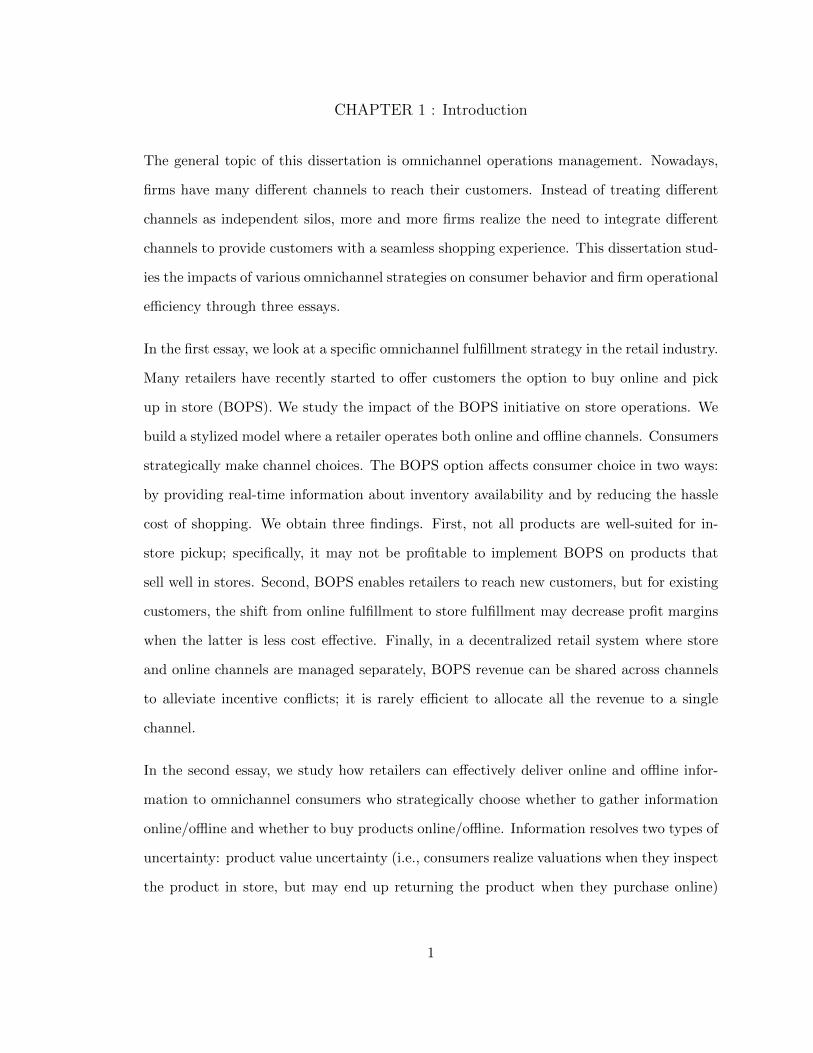
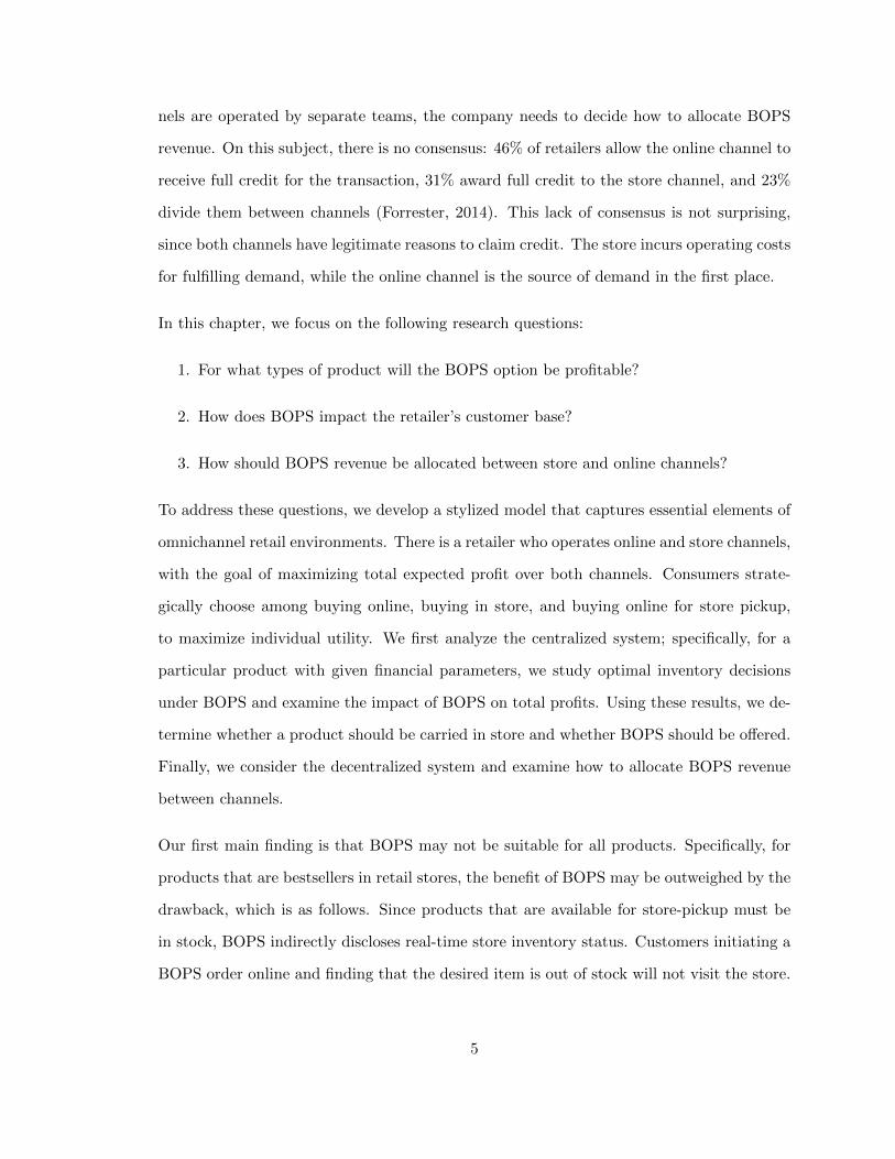
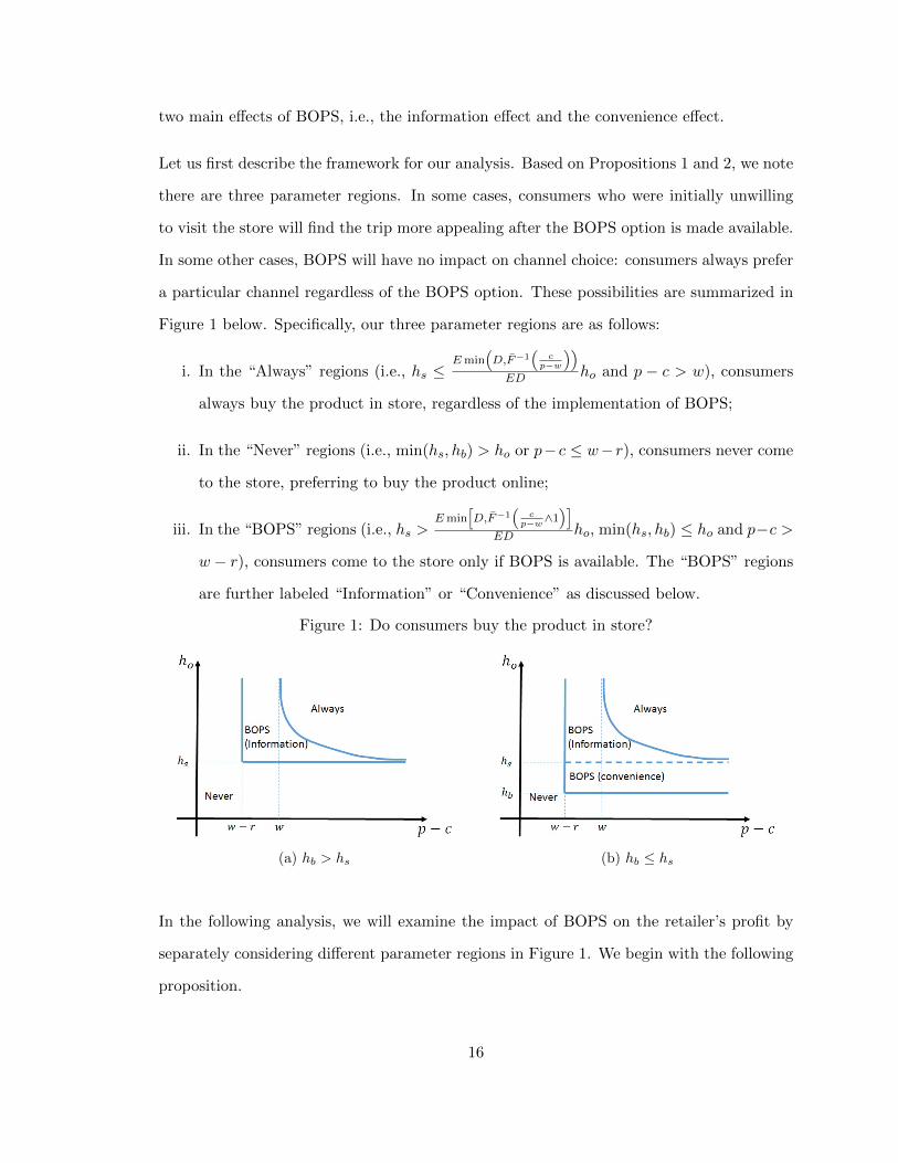
Figure 1 below. Specifically, our three parameter regions are as follows:
i. In the “Always” regions (i.e., hs ≤Emin
(D,F−1
(c
p−w
))ED ho and p − c > w), consumers
always buy the product in store, regardless of the implementation of BOPS;
ii. In the “Never” regions (i.e., min(hs, hb) > ho or p− c ≤ w−r), consumers never come
to the store, preferring to buy the product online;
iii. In the “BOPS” regions (i.e., hs >Emin
[D,F−1
(c
p−w∧1)]
ED ho, min(hs, hb) ≤ ho and p−c >
w − r), consumers come to the store only if BOPS is available. The “BOPS” regions
are further labeled “Information” or “Convenience” as discussed below.
Figure 1: Do consumers buy the product in store?
(a) hb > hs (b) hb ≤ hs
In the following analysis, we will examine the impact of BOPS on the retailer’s profit by
separately considering different parameter regions in Figure 1. We begin with the following
proposition.
16
Proposition 3. If hs ∈
(Emin
[D,F−1
(c
p−w∧1)]
ED ho, ho
]and p−c > w−r, then customers visit
the store only if BOPS is available. Further, BOPS increases total profit (i.e., π∗ > π◦).
The conditions in Proposition 3 correspond to the “BOPS” regions labeled “Information”
in Figures 1a and 1b. In these parameter regions, BOPS influences consumer shopping
behavior through the information sharing mechanism discussed in the previous section.
By revealing real-time information about store inventory status, BOPS draws additional
customers to the store; these customers were previously unwilling to visit the store because
they were discouraged by the possibility of stockouts. In such cases, Proposition 3 confirms
that BOPS leads to increased profit for the retailer. This increase in profit arises because
the store profit margin p− c, combined with the cross-selling benefit r, exceeds the online
margin w. In other words, through information provision, BOPS brings about a demand
shift to the more profitable store channel.
There is a subtle difference between the two “BOPS (Information)” regions of Figures 1a
and 1b. Although demand shifts to the store in both cases, they occur in different ways.
In the “BOPS (Information)” region of Figure 1a, since the pickup hassle cost hb exceeds
the store hassle cost hs, offering BOPS induces consumers to buy in store after verifying
availability online, without actually using the BOPS functionality. On the other hand, in
the corresponding region of Figure 1b, consumers indeed buy online and pick up in store
when the option is available. We separately discuss these two behaviors in the next two
paragraphs.
When consumers verify availability online without actually using the BOPS functionality,
BOPS simply serves as a source of information. The same market outcome arises if the re-
tailer simply provides real-time availability information on the website (i.e., directly showing
whether or not store is in stock). This strategy has been adopted by retailers such as Gap
and Levi’s. Our model can be applied to study this pure information sharing mechanism,
which can be regarded as a special case with hb > hs. In this special case, BOPS generates
17
an interesting dynamic: after the implementation of BOPS as an added online functional-
ity, online sales may decrease, while store sales may increase. This phenomenon was first
identified by Gallino and Moreno (2014), who undertake a comprehensive empirical study
of a US retailer with a recent BOPS implementation.
On the other hand, when the pickup process is relatively hassle-free, consumers will indeed
buy online and pick up in store. In this case, apart from eliminating the risk of stockouts as
described above, BOPS also provides consumers with a more convenient means of shopping.
In this sense, comparing the two “BOPS (Information)” regions in Figures 1a and 1b,
consumer surplus is higher in the latter than in the former.
The next proposition examines the “BOPS” region labeled “Convenience” in Figure 1b.
Proposition 4. If hb ≤ ho < hs and p− c > w− r, customers visit the store only if BOPS
is available. Further, BOPS increases total profit (i.e., π∗ > π◦).
The above result highlights the importance of shopping convenience for BOPS to attract
consumers to the store. By additionally providing convenience, BOPS becomes more pow-
erful than a pure information sharing mechanism. In the “BOPS (Convenience)” region of
Figure 1b, a pure information sharing mechanism can never attract customers to the store;
even if customers are guaranteed availability in store, they still prefer to buy online because
the online hassle cost is lower than the store hassle cost (i.e., ho < hs). However, once
BOPS is available and provides convenience that trumps an online order (i.e., hb < ho),
customers may prefer to buy online and pick up in store. This shopping mode benefits the
retailer because customers may buy additional products (yielding profit r) when they pick
up their products. As long as the store margin p− c and cross-selling benefit r exceeds the
online margin w, the convenience dimension of BOPS will lead to increased profit for the
retailer.
Proposition 4 provides a word of caution for retailers. Although making the pickup process
more convenient is potentially a good way to improve the profitability of BOPS, retailers
18
should exercise care in preserving the cross-selling benefit. In particular, some retailers
have introduced drive-through service that allows customers to receive their orders without
leaving their cars (New York Times, 2012; Bloomberg, 2012). Although this will help to
reduce hassle in the pickup process, it will also prevent people from entering the store and
thus lead to a loss of the cross-selling benefit r. According to Proposition 4, if the margin
from selling this particular product in the store is very high (i.e., p − c > w), then it is
still profitable for the retailer to implement BOPS even if r = 0. However, if profit margins
are lower in store than online, then the cross-selling profit r plays an important role; in
this case, drive-through service may hurt the retailer’s overall profit by neutralizing the
advantages of cross-selling.
There is a delicate balance between pickup convenience and cross-selling potential. While
consumers appreciate a more convenient pickup process, retail managers wishing to make
the most out of the cross-selling opportunity may choose to locate the pick-up counter at
far corners of the store so that shoppers have to walk through the entire store before picking
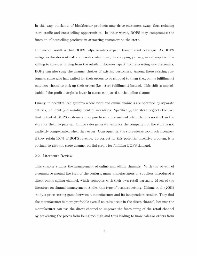
up their online orders (Retail Dive, 2015). This tradeoff is illustrated in Figure 2. At one
extreme, setting the pickup counter at the back of store maximizes both pickup cost hb
and cross-selling benefit r (i.e., the dotted L-line). At the other extreme, providing drive
through pickup service minimizes both hb and r (i.e., the dashed L-line). As both hb and
r increase, the L-line in Figure 1 moves up and left, and the “BOPS” region changes. The
optimal location of the L curve depends on retailer’s portfolio of products. According to
Figure 2, if most of the retailer’s products have high store profit margins (i.e., p−c is large)
and can be easily purchased online (i.e., ho is small), then the retailer should seek to make
the pickup process more convenient; in contrast, if most of the retailer’s products have low
store profit margins (i.e., p−c is small) and are difficult to purchase online (i.e., ho is large),
then setting the pickup counter far from the store entrance is a better strategy.
The next proposition tells a different side of the story. Although BOPS brings about many
benefits, it may lead to reduced profits in some cases.
19
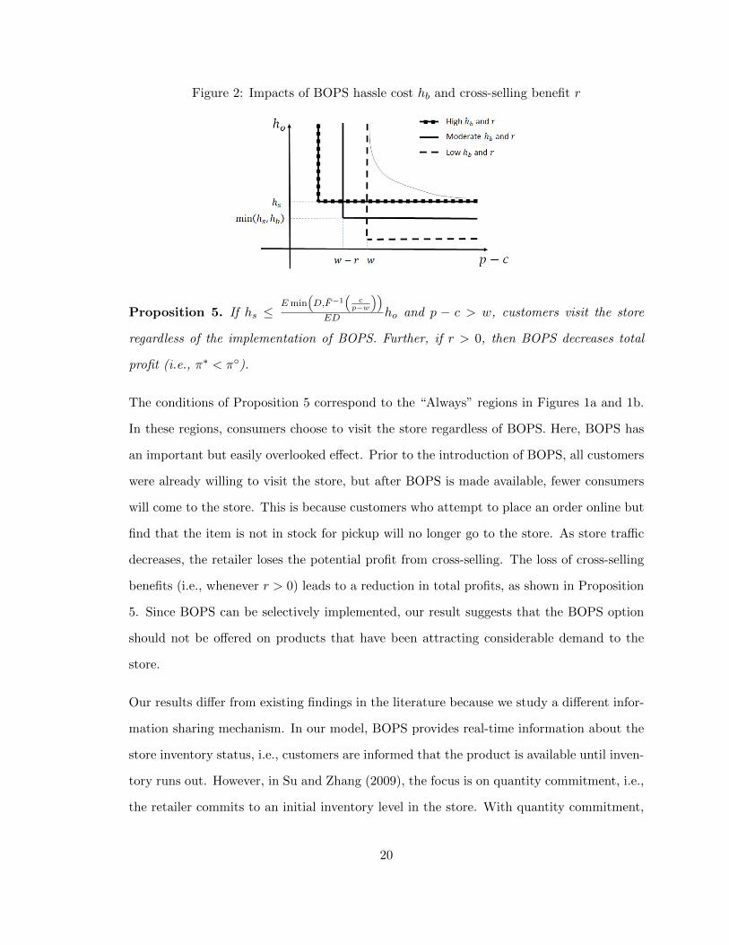
Figure 2: Impacts of BOPS hassle cost hb and cross-selling benefit r
Proposition 5. If hs ≤Emin
(D,F−1
(c
p−w
))ED ho and p − c > w, customers visit the store
regardless of the implementation of BOPS. Further, if r > 0, then BOPS decreases total
profit (i.e., π∗ < π◦).
The conditions of Proposition 5 correspond to the “Always” regions in Figures 1a and 1b.
In these regions, consumers choose to visit the store regardless of BOPS. Here, BOPS has
an important but easily overlooked effect. Prior to the introduction of BOPS, all customers
were already willing to visit the store, but after BOPS is made available, fewer consumers
will come to the store. This is because customers who attempt to place an order online but
find that the item is not in stock for pickup will no longer go to the store. As store traffic
decreases, the retailer loses the potential profit from cross-selling. The loss of cross-selling
benefits (i.e., whenever r > 0) leads to a reduction in total profits, as shown in Proposition
5. Since BOPS can be selectively implemented, our result suggests that the BOPS option
should not be offered on products that have been attracting considerable demand to the
store.
Our results differ from existing findings in the literature because we study a different infor-
mation sharing mechanism. In our model, BOPS provides real-time information about the
store inventory status, i.e., customers are informed that the product is available until inven-
tory runs out. However, in Su and Zhang (2009), the focus is on quantity commitment, i.e.,
the retailer commits to an initial inventory level in the store. With quantity commitment,
20
the retailer may be able to use a small amount of store inventory to attract a large number
of customers to visit the store. In particular, when the cross-selling benefit is very large, the
retailer may still choose to stock the product in the store even if it is more profitable to sell
online, with the hope of attracting customers to make additional purchases in store. Such
a “loss leader strategy” is no longer feasible when the retailer implements BOPS, because
customers have access to real-time store inventory information and will not visit the store
after the product is out of stock. Therefore, we find that BOPS, by providing real-time
inventory information, may decrease profits, while Su and Zhang (2009) find that quantity
commitment is generally valuable.
In summary, BOPS has two effects: it provides customers with real-time information about
in-store inventory availability and it introduces a new shopping mode that may add conve-
nience to customers. The former effect (information effect) helps attract customers to the
store by letting them know about inventory availability, but it is a double-edged sword in
that when inventory is not available, it turns away customers who might be willing to visit
the store. The latter effect (convenience effect) applies when customers use the store pickup
functionality, as opposed to simply using BOPS as a source of availability information; it
draws customers to the store and may even open up new sources of demand.
When put together, the information and convenience effects of BOPS yield different profit
implications. Figures 1a and 1b present a clear distinction: in the “BOPS” regions, BOPS
leads to higher profits, but in the “Always” regions, BOPS leads to lower profits. The
difference between these two regions is that, prior to the introduction of BOPS, consumers
were already willing to visit the store in the latter but not in the former. These results
suggest that BOPS should be offered for products with weak store sales but not those with
strong records to begin with. In other words, it is likely profitable to implement BOPS on
in-store “underdogs” but may not be so for in-store “favorites.”
21
2.5. Heterogeneous Customers
In this section, we incorporate customer heterogeneity. For example, some customers may
reside further away from the store than others; some may be more impatient than others
and are thus more averse to waiting for online delivery. In our model, the store and online
hassle costs hs, ho may now differ across customers. Specifically, customers are uniformly
distributed across the following “square” {(hs, ho)|hs ∈ [0, H], ho ∈ [0, H]}, where H > v−p
(i.e., some customers have a prohibitively high hassle cost in one channel). The goal is to
study the impact of BOPS on a retailer’s customer base in such a heterogeneous market.
We begin by considering the scenario in the absence of BOPS. In this case, each customer
has three options: go to the store, buy online, or leave the market. The corresponding
utilities are:
us = −hs + ξ(v − p) + (1− ξ)u+o ,
uo = v − p− ho,
ul = 0,
where ξ denotes the belief about store inventory availability as before. Note that customers
who find the store out of stock will buy online only if doing so is preferred over leaving the
market. As customers make utility-maximizing choices (which depend on their hassle costs
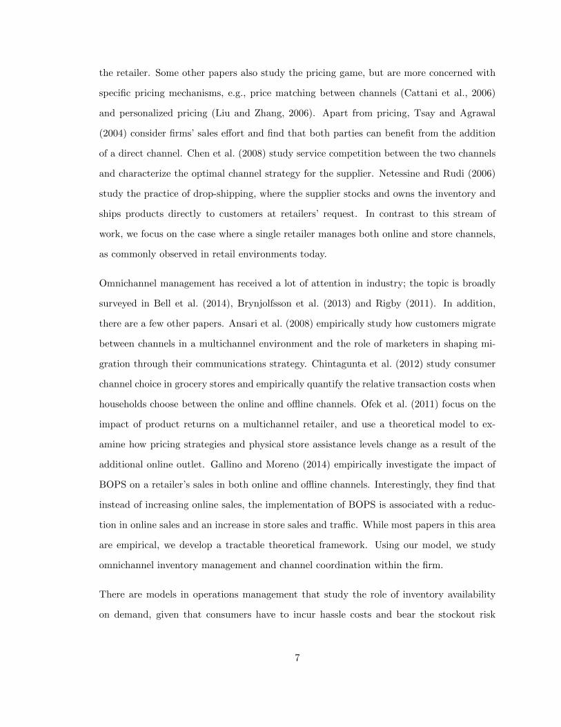
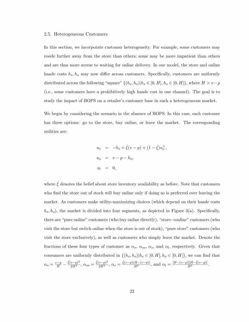
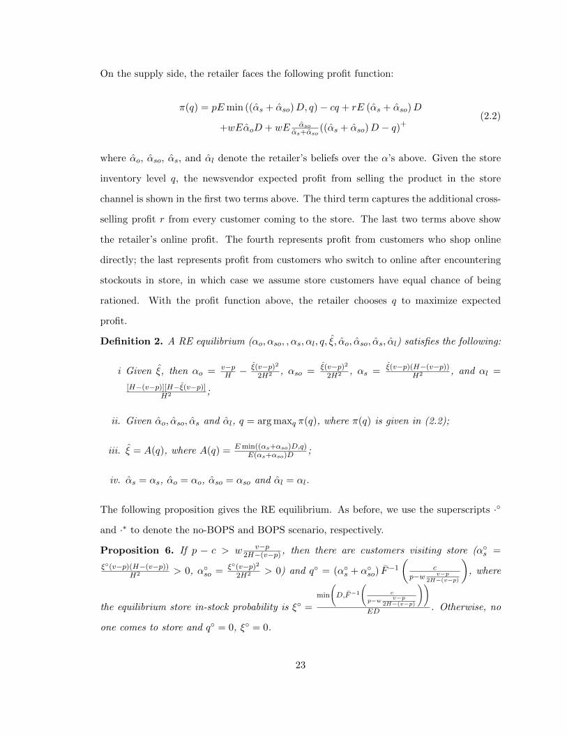
hs, ho), the market is divided into four segments, as depicted in Figure 3(a). Specifically,
there are “pure online” customers (who buy online directly), “store→online” customers (who
visit the store but switch online when the store is out of stock), “pure store” customers (who
visit the store exclusively), as well as customers who simply leave the market. Denote the
fractions of these four types of customer as αo, αso, αs, and αl, respectively. Given that
consumers are uniformly distributed in {(hs, ho)|hs ∈ [0, H], ho ∈ [0, H]}, we can find that
αo = v−pH − ξ(v−p)2
2H2 , αso = ξ(v−p)2
2H2 , αs = ξ(v−p)(H−(v−p))H2 , and αl = [H−(v−p)][H−ξ(v−p)]
H2 .
22
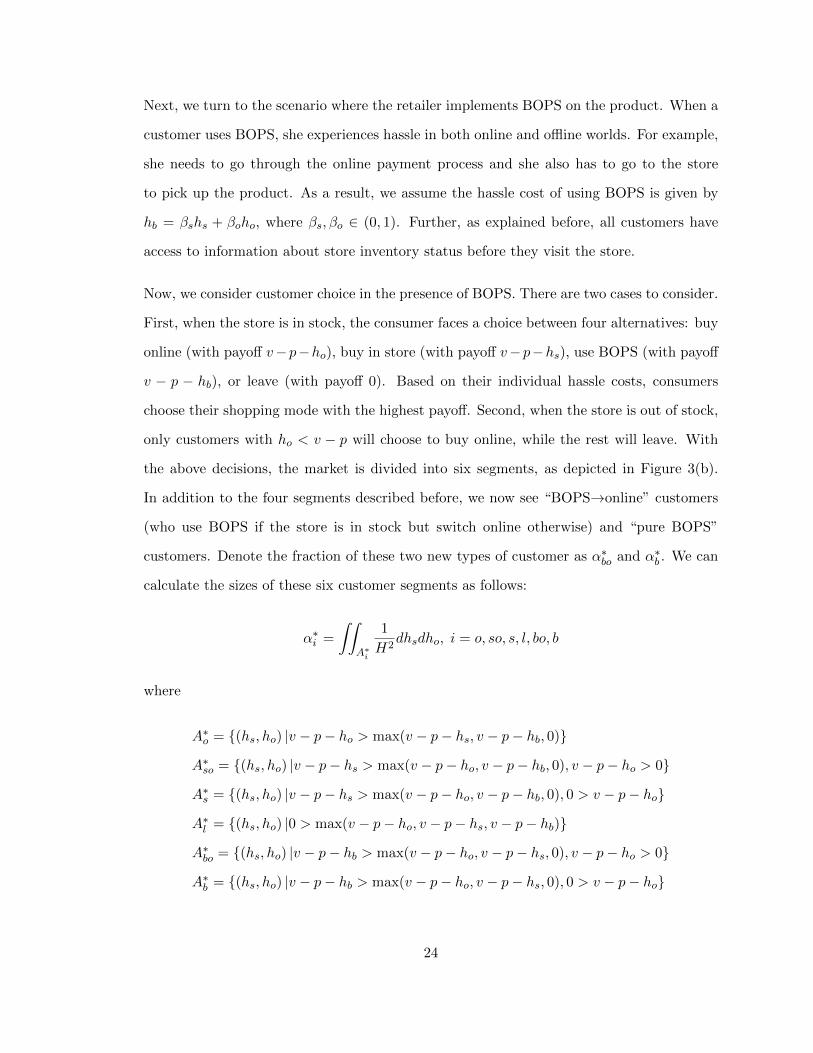
On the supply side, the retailer faces the following profit function:
π(q) = pEmin ((αs + αso)D, q)− cq + rE (αs + αso)D
+wEαoD + wE αsoαs+αso
((αs + αso)D − q)+(2.2)
where αo, αso, αs, and αl denote the retailer’s beliefs over the α’s above. Given the store
inventory level q, the newsvendor expected profit from selling the product in the store
channel is shown in the first two terms above. The third term captures the additional cross-
selling profit r from every customer coming to the store. The last two terms above show
the retailer’s online profit. The fourth represents profit from customers who shop online
directly; the last represents profit from customers who switch to online after encountering
stockouts in store, in which case we assume store customers have equal chance of being
rationed. With the profit function above, the retailer chooses q to maximize expected
profit.
Definition 2. A RE equilibrium (αo, αso, , αs, αl, q, ξ, αo, αso, αs, αl) satisfies the following:
i Given ξ, then αo = v−pH − ξ(v−p)2
2H2 , αso = ξ(v−p)2
2H2 , αs = ξ(v−p)(H−(v−p))H2 , and αl =
[H−(v−p)][H−ξ(v−p)]H2 ;
ii. Given αo, αso, αs and αl, q = arg maxq π(q), where π(q) is given in (2.2);
iii. ξ = A(q), where A(q) = Emin((αs+αso)D,q)E(αs+αso)D
;
iv. αs = αs, αo = αo, αso = αso and αl = αl.
The following proposition gives the RE equilibrium. As before, we use the superscripts ·◦
and ·∗ to denote the no-BOPS and BOPS scenario, respectively.
Proposition 6. If p − c > w v−p2H−(v−p) , then there are customers visiting store (α◦s =
ξ◦(v−p)(H−(v−p))H2 > 0, α◦so = ξ◦(v−p)2
2H2 > 0) and q◦ = (α◦s + α◦so) F−1
(c
p−w v−p2H−(v−p)
), where
the equilibrium store in-stock probability is ξ◦ =
min
(D,F−1
(c
p−w v−p2H−(v−p)
))ED . Otherwise, no
one comes to store and q◦ = 0, ξ◦ = 0.
23
Next, we turn to the scenario where the retailer implements BOPS on the product. When a
customer uses BOPS, she experiences hassle in both online and offline worlds. For example,
she needs to go through the online payment process and she also has to go to the store
to pick up the product. As a result, we assume the hassle cost of using BOPS is given by
hb = βshs + βoho, where βs, βo ∈ (0, 1). Further, as explained before, all customers have
access to information about store inventory status before they visit the store.
Now, we consider customer choice in the presence of BOPS. There are two cases to consider.
First, when the store is in stock, the consumer faces a choice between four alternatives: buy
online (with payoff v−p−ho), buy in store (with payoff v−p−hs), use BOPS (with payoff
v − p − hb), or leave (with payoff 0). Based on their individual hassle costs, consumers
choose their shopping mode with the highest payoff. Second, when the store is out of stock,
only customers with ho < v − p will choose to buy online, while the rest will leave. With
the above decisions, the market is divided into six segments, as depicted in Figure 3(b).
In addition to the four segments described before, we now see “BOPS→online” customers
(who use BOPS if the store is in stock but switch online otherwise) and “pure BOPS”
customers. Denote the fraction of these two new types of customer as α∗bo and α∗b . We can
calculate the sizes of these six customer segments as follows:
α∗i =
∫∫A∗i
1
H2dhsdho, i = o, so, s, l, bo, b
where
A∗o = {(hs, ho) |v − p− ho > max(v − p− hs, v − p− hb, 0)}
A∗so = {(hs, ho) |v − p− hs > max(v − p− ho, v − p− hb, 0), v − p− ho > 0}
A∗s = {(hs, ho) |v − p− hs > max(v − p− ho, v − p− hb, 0), 0 > v − p− ho}
A∗l = {(hs, ho) |0 > max(v − p− ho, v − p− hs, v − p− hb)}
A∗bo = {(hs, ho) |v − p− hb > max(v − p− ho, v − p− hs, 0), v − p− ho > 0}
A∗b = {(hs, ho) |v − p− hb > max(v − p− ho, v − p− hs, 0), 0 > v − p− ho}
24
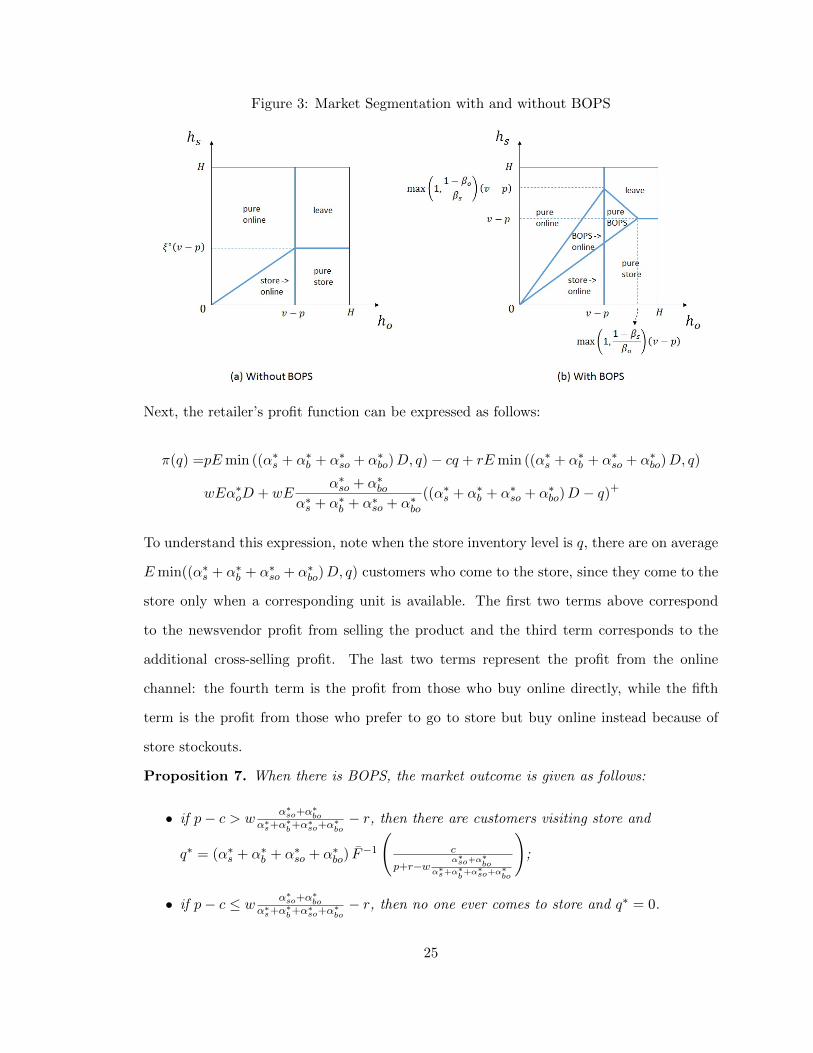
Figure 3: Market Segmentation with and without BOPS
Next, the retailer’s profit function can be expressed as follows:
π(q) =pEmin ((α∗s + α∗b + α∗so + α∗bo)D, q)− cq + rEmin ((α∗s + α∗b + α∗so + α∗bo)D, q)
wEα∗oD + wEα∗so + α∗bo
α∗s + α∗b + α∗so + α∗bo((α∗s + α∗b + α∗so + α∗bo)D − q)
+
To understand this expression, note when the store inventory level is q, there are on average
Emin((α∗s + α∗b + α∗so + α∗bo)D, q) customers who come to the store, since they come to the
store only when a corresponding unit is available. The first two terms above correspond
to the newsvendor profit from selling the product and the third term corresponds to the
additional cross-selling profit. The last two terms represent the profit from the online
channel: the fourth term is the profit from those who buy online directly, while the fifth
term is the profit from those who prefer to go to store but buy online instead because of
store stockouts.
Proposition 7. When there is BOPS, the market outcome is given as follows:
• if p− c > wα∗so+α
∗bo
α∗s+α∗b+α∗so+α∗bo− r, then there are customers visiting store and
q∗ = (α∗s + α∗b + α∗so + α∗bo) F−1
(c
p+r−wα∗so+α∗
boα∗s+α∗
b+α∗so+α∗
bo
);
• if p− c ≤ w α∗so+α∗bo
α∗s+α∗b+α∗so+α∗bo− r, then no one ever comes to store and q∗ = 0.
25
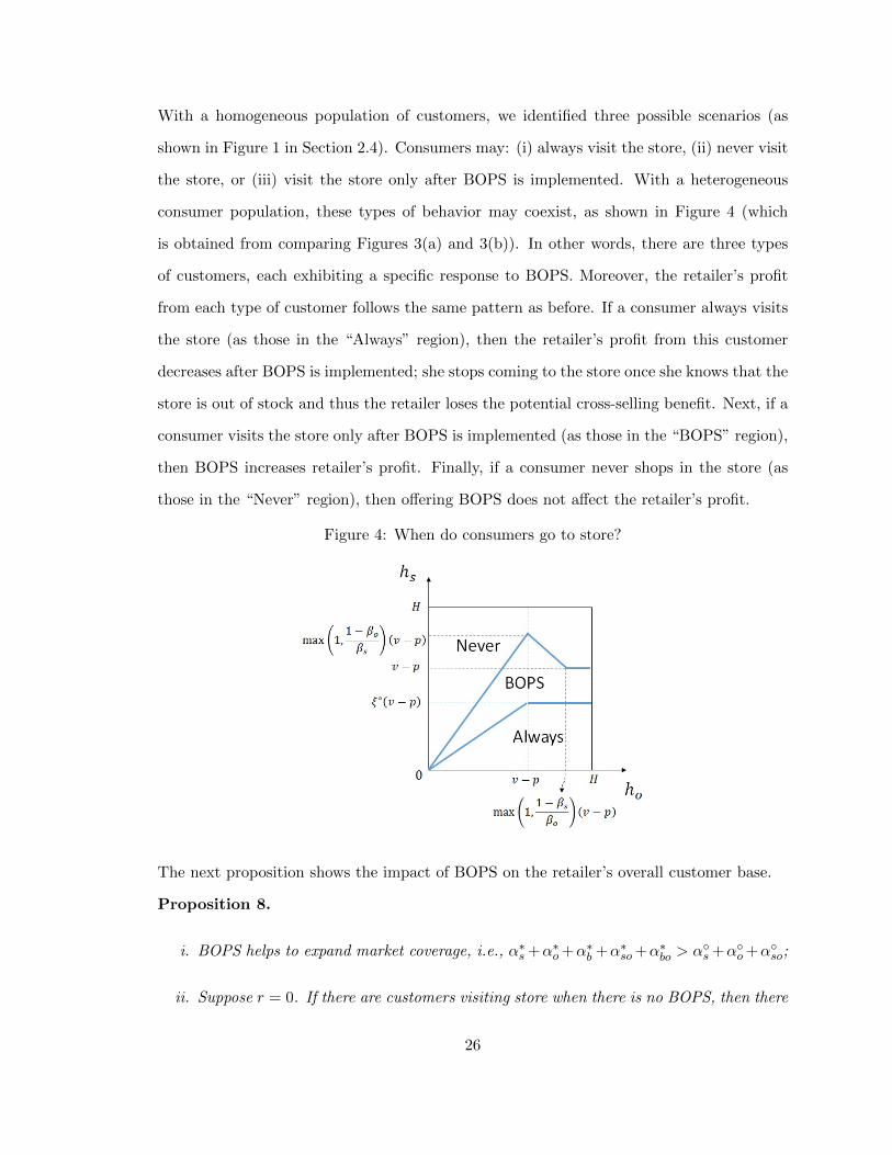
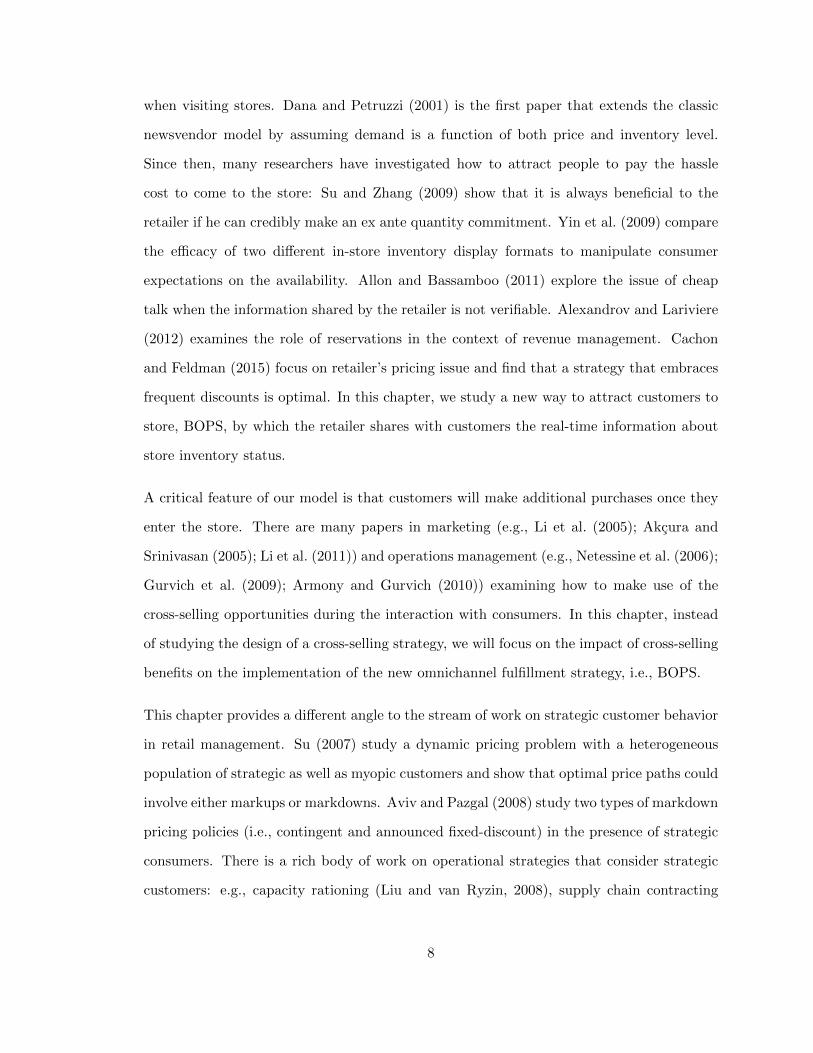
With a homogeneous population of customers, we identified three possible scenarios (as
shown in Figure 1 in Section 2.4). Consumers may: (i) always visit the store, (ii) never visit
the store, or (iii) visit the store only after BOPS is implemented. With a heterogeneous
consumer population, these types of behavior may coexist, as shown in Figure 4 (which
is obtained from comparing Figures 3(a) and 3(b)). In other words, there are three types
of customers, each exhibiting a specific response to BOPS. Moreover, the retailer’s profit
from each type of customer follows the same pattern as before. If a consumer always visits
the store (as those in the “Always” region), then the retailer’s profit from this customer
decreases after BOPS is implemented; she stops coming to the store once she knows that the
store is out of stock and thus the retailer loses the potential cross-selling benefit. Next, if a
consumer visits the store only after BOPS is implemented (as those in the “BOPS” region),
then BOPS increases retailer’s profit. Finally, if a consumer never shops in the store (as
those in the “Never” region), then offering BOPS does not affect the retailer’s profit.
Figure 4: When do consumers go to store?
The next proposition shows the impact of BOPS on the retailer’s overall customer base.
Proposition 8.
i. BOPS helps to expand market coverage, i.e., α∗s +α∗o +α∗b +α∗so+α∗bo > α◦s +α◦o +α◦so;
ii. Suppose r = 0. If there are customers visiting store when there is no BOPS, then there
26
exists w such that the implementation of BOPS decreases total profit (i.e., π∗ < π◦)
if βs + βo < 1 and w > w.
Before BOPS is implemented, customers who face high hassle costs in both store and online
channels do not consider purchasing from the retailer. Part (i) of Proposition 8 shows that
BOPS could provide a way for the retailer to reach these customers. By alleviating the risk
of stockouts and reducing the hassle of shopping, BOPS could attract some new customers
to join the market. This market expansion effect could also be seen from the reduction of
the “leave” region in Figure 3(b) compared to Figure 3(a).
While reaching out to new customers, BOPS may change the behavior of existing customers.
Specifically, the more convenient BOPS is, the more existing online customers will choose
to pick up their orders in store; this shift will hurt profits if the store profit margin is lower
than the online profit margin. This potential drawback of BOPS may exist even when r = 0,
as shown in Proposition 8(ii). In other words, apart from possibly eliminating cross-selling
opportunities (when r > 0) as discovered earlier, BOPS has another potential drawback of
shifting demand to a less profitable store channel.
2.6. Decentralized System
In this section, we study the scenario where the store and online channels are operated by
two separate teams, with the goal of understanding how BOPS revenue should be allocated.
We begin by examining the case with homogeneous customers and then later extrapolate our
findings to the case with heterogeneous customers. (A detailed analysis of the decentralized
system for the heterogeneous market is given in Appendix A.1.) We assume that the
conditions in Proposition 2 hold (i.e., min(hs, hb) ≤ ho and p− c > w− r) and BOPS hassle
cost is lowest (i.e., hb < min(hs, ho)); otherwise, there would be nobody using BOPS and the
issue of revenue allocation becomes irrelevant as the system collapses into two independent
channels.
We use θ ∈ [0, 1] to denote the share of BOPS revenue that the store obtains. In other
27
words, for every customer who purchases online and picks up in the store, the store earns
θp from selling the product. Note that once the customer comes to the store, the store could
also get an additional profit r through cross-selling. Therefore, the total revenue that the
store could receive from fulfilling each unit of BOPS demand is θp + r. Then, the store’s
expected profit as a function of the stocking decision q is given below. Here, we use the
“tilde” symbol (·) to denote the decentralized case.
πs = (θp+ r)Emin (D, q)− cq
Proposition 9. In the decentralized system, the store will stock q∗ which is given as follows:
• If θp+ r − c > 0, then q∗ = F−1(
cθp+r
);
• If θp+ r − c ≤ 0, then q∗ = 0.
In practice, according to the survey conducted by Forrester Research (Forrester, 2014), the
two most common revenue sharing schemes are either giving the store full credit (i.e., θ = 1)
or letting the online channel keep all the revenue (i.e., θ = 0). According to Proposition 9,
when θ = 1, the store will definitely stock the product to serve BOPS users, because he can
not only receive a positive profit margin from selling this particular product, but he may
also be able to cross sell other products to those who come to store for pickup. However, if
θ = 0, BOPS customers represent a pure cost to the store; then, the store may choose not
to stock the product in store, unless the cross-selling benefit is large enough to offset the
loss from serving BOPS customers (i.e., r > c).
What is the optimal share of BOPS revenue that should be allocated to the store? We
use π∗(θ) to denote total profit in the decentralized system with revenue allocation θ.
For any given θ, the next proposition compares decentralized and centralized inventory
decisions and shows that the store is usually either overstocked or understocked, relative to
the centralized benchmark. However, there is an optimal revenue share, under which the
decentralized system achieves the centralized optimal profit.
28
Proposition 10. Total profit π∗(θ) is quasiconcave in θ. Moreover,
• if θ < p−wp , then q∗ < q∗ and π∗(θ) < π∗;
• if θ = p−wp , then q∗ = q∗ and π∗(θ) = π∗;
• if θ > p−wp , then q∗ > q∗ and π∗(θ) < π∗.
Proposition 10 points out an incentive conflict between the store channel and the retail
organization. If the store channel obtains a large share of BOPS revenue, they tend to
stock too much. This is because the store channel considers only store profits but neglects
the fact that customers may still be willing to shop online after the store runs out of
inventory for customers to pick up. In contrast, if the store is allocated only a small share
of BOPS revenue, they tend to stock too little. Since the store channel incurs the inventory
cost for fulfilling BOPS demand, it is natural to suppress inventory to decrease exposure
to potential losses. In general, it is optimal to give the store partial credit for the revenue
earned from BOPS customers. In fact, our result also shows that such a simple revenue
sharing mechanism is sufficient for the retailer to fully coordinate the store and online
channels.
Proposition 10 shows that the optimal revenue share θ∗ = p−wp coordinates the decentralized
system and achieves the centralized optimal profit π∗. With this optimal revenue share,
the incentives of the store channel are aligned with the entire organization. According to
Proposition 9, the decentralized store channel holds stock if and only if θp + r − c > 0.
However, from the perspective of the entire organization, as we have shown in the previous
section, it is optimal to stock the product in the store as long as p−c > w−r, i.e., whenever
the store margin p− c, combined with the cross-selling benefit r, exceeds the online margin
w. The revenue share θ that aligns both sets of incentives is precisely θ∗ = p−wp .
Note that the optimal share for the store channel θ∗ = p−wp is decreasing in w. The reason
is as follows. As the online margin w increases, it becomes more profitable to sell through
29
the online channel. However, in the absence of BOPS, the store will continue to stock the
same amount of inventory since they tend to neglect the profit from online orders. Through
sharing the BOPS revenue, the retail organization has a natural way to correct for the
misaligned incentive. By allocating less revenue to the store channel for fulfilling BOPS
demand, the retail organization can induce the store channel to lower their inventory level.
This compensates for the incentive conflict and allows more demand to flow to the more
profitable online channel.
Although Proposition 10 shows that the optimal revenue sharing mechanism will achieve
full centralized profits in a homogeneous market, Appendix A.1 presents a different result
for a heterogeneous market. Specifically, when the proportion of customers who use the
BOPS functionality is too low, the amount of BOPS revenue to be shared between the
channels may be insignificant and as a result, a simple revenue sharing mechanism cannot
fully coordinate the omnichannel retail system. The analysis in Appendix A.1 highlights
the benefit as more customers adopt BOPS: the increased stream of BOPS revenue can
provide headquarters with more leverage to alleviate incentive conflicts between the store
and online channels.
Omnichannel retailers who recognize the incentive conflicts brought about by BOPS have
begun to experiment with simple revenue sharing schemes. A common and simple approach
is to assign full credit for the sale of a BOPS item to both store and online channels. In other
words, there is some double counting on internal books that are subsequently adjusted for.
Depending on accounting protocols, this method is usually akin to allocating equal revenue
shares to each channel. Since the optimal revenue share may not be 50%, the simple
heuristic described above has room for improvement, and our analysis provides a possible
way to think about how to do so.
In practice, a retailer may carry a large number of SKUs with different prices and margins.
Admittedly, it would be impractical to set a different revenue sharing parameter θ for each
SKU. Instead, a retailer may want to have a common θ for a group of products. In such
30
case, since the optimal profit function π∗(θ) is quasiconcave in θ, the optimal θ∗’s given in
Proposition 10 for the group of products could serve as benchmarks for the retailer to find
a common compromise θ that is close enough to each of the different θ∗’s.
2.7. Conclusion
In this chapter, we study a specific omnichannel fulfillment strategy: buy-online-and-pick-
up-in-store (BOPS). We develop a stylized model that captures essential elements of om-
nichannel retail environments; in particular, consumers strategically choose channels for
purchase and fulfillment. We find that BOPS attracts consumer demand through an in-
formation effect and a convenience effect. The former effect arises because BOPS reveals
real-time information about store inventory availability. Products that are available for
store-pickup must be in stock. With this assurance, customers are more willing to visit
the store. The latter effect arises because BOPS offers a new and possibly more conve-
nient mode of shopping. By helping consumers pick out items and move them to checkout
counters, BOPS reduces the hassle of shopping.
Even though BOPS is a popular fulfillment option among consumers, we find that retailers
need to be cautious when implementing it. Retailers can benefit from this new fulfillment
strategy by being selective when choosing the set of products eligible for in-store pickup.
BOPS can help attract more customers to the store and thus boost the sales of products
that were previously not selling well; however, for store bestsellers, offering the BOPS option
may have the unintended consequence of reducing store traffic. Moreover, although BOPS
can be a good strategy for a retailer to build up its customer base, BOPS may at the same
time drive existing online customers to the store channel where the profit margin might
be lower compared to the online channel. Finally, retailers with decentralized operations
can maximize profits by allocating BOPS revenue between the online and store channels
appropriately, and giving full credit to either channel is seldom optimal.
To simplify the analysis, we have imposed two assumptions in our model: (1) The online
31
channel is exogenous and always in stock, and (2) all customers check the information online
when BOPS is offered. As robustness checks, we have built two model extensions to relax
the assumptions above. Specifically, in Appendix A.2.1, we consider the case where the
retailer has limited inventory in both the store and online channels; in Appendix A.2.2,
we consider customers who simply head to the store by default (e.g., they may forget or
simply not care to check websites beforehand). Our key results remain valid in these model
extensions.
Beyond the scope of our current analysis is the potential impact of BOPS on operational
costs. On the one hand, BOPS helps to reduce online shipping costs since it transfers the
burden of last-mile delivery to customers. On the other hand, BOPS is accompanied by
new fulfillment responsibilities wherein a retailer’s comparative advantage may not lie. For
example, stores need to train their workforce to perform pick-and-pack tasks in a timely
fashion (Forrester, 2014), and to handle increased demand, stores need to hire more employ-
ees to deal with online orders (Business Insider, 2012). A more careful cost-based analysis
of BOPS is left as an interesting topic for future research.
The omnichannel strategy discussed in this chapter, BOPS, addresses purchases that origi-
nate online but are completed in the store. In the spirit of Bell et al. (2014), who provide
a framework for omnichannel retail, BOPS customers receive information online but their
demand is fulfilled in the store. The reverse type of shopping behavior is where customers
research the product in stores and then shop online, usually at lower prices. This is known
as showrooming behavior and has been critiqued widely: showroomers and e-tailers are ac-
cused of free-riding on inventory displays at brick-and-mortar stores (Wall Street Journal,
2012b,a). Recent research by Balakrishnan et al. (2014) shows that showrooming behavior
intensifies retail competition, and Mehra et al. (2013) studies how a brick-and-mortar re-
tailer can counteract showrooming behavior through strategies such as price matching and
retail club memberships. Taking the e-tailer’s perspective, Bell et al. (2015) empirically
studies the value of providing offline showrooms to mitigate customer uncertainty. We hope
32
that our model in this chapter can contribute to this exciting line of research.
33
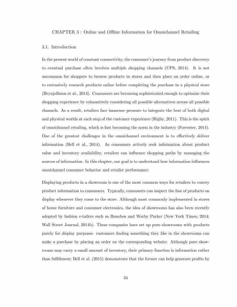
CHAPTER 3 : Online and Offline Information for Omnichannel Retailing
3.1. Introduction
In the present world of constant connectivity, the consumer’s journey from product discovery
to eventual purchase often involves multiple shopping channels (UPS, 2014). It is not
uncommon for shoppers to browse products in stores and then place an order online, or
to extensively research products online before completing the purchase in a physical store
(Brynjolfsson et al., 2013). Consumers are becoming sophisticated enough to optimize their
shopping experience by exhaustively considering all possible alternatives across all possible
channels. As a result, retailers face immense pressure to integrate the best of both digital
and physical worlds at each step of the customer experience (Rigby, 2011). This is the spirit
of omnichannel retailing, which is fast becoming the norm in the industry (Forrester, 2014).
One of the greatest challenges in the omnichannel environment is to effectively deliver
information (Bell et al., 2014). As consumers actively seek information about product
value and inventory availability, retailers can influence shopping paths by managing the
sources of information. In this chapter, our goal is to understand how information influences
omnichannel consumer behavior and retailer performance.
Displaying products in a showroom is one of the most common ways for retailers to convey
product information to consumers. Typically, consumers can inspect the line of products on
display whenever they come to the store. Although most commonly implemented in stores
of home furniture and consumer electronics, the idea of showrooms has also been recently
adopted by fashion e-tailers such as Bonobos and Warby Parker (New York Times, 2014;
Wall Street Journal, 2014b). These companies have set up pure showrooms with products
purely for display purposes: customers finding something they like in the showrooms can
make a purchase by placing an order on the corresponding website. Although pure show-
rooms may carry a small amount of inventory, their primary function is information rather
than fulfillment; Bell et al. (2015) demonstrate that the former can help generate profits by
34
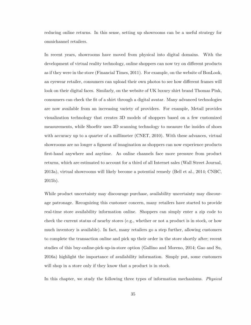
reducing online returns. In this sense, setting up showrooms can be a useful strategy for
omnichannel retailers.
In recent years, showrooms have moved from physical into digital domains. With the
development of virtual reality technology, online shoppers can now try on different products
as if they were in the store (Financial Times, 2011). For example, on the website of BonLook,
an eyewear retailer, consumers can upload their own photos to see how different frames will
look on their digital faces. Similarly, on the website of UK luxury shirt brand Thomas Pink,
consumers can check the fit of a shirt through a digital avatar. Many advanced technologies
are now available from an increasing variety of providers. For example, Metail provides
visualization technology that creates 3D models of shoppers based on a few customized
measurements, while Shoefitr uses 3D scanning technology to measure the insides of shoes
with accuracy up to a quarter of a millimeter (CNET, 2010). With these advances, virtual
showrooms are no longer a figment of imagination as shoppers can now experience products
first-hand anywhere and anytime. As online channels face more pressure from product
returns, which are estimated to account for a third of all Internet sales (Wall Street Journal,
2013a), virtual showrooms will likely become a potential remedy (Bell et al., 2014; CNBC,
2015b).
While product uncertainty may discourage purchase, availability uncertainty may discour-
age patronage. Recognizing this customer concern, many retailers have started to provide
real-time store availability information online. Shoppers can simply enter a zip code to
check the current status of nearby stores (e.g., whether or not a product is in stock, or how
much inventory is available). In fact, many retailers go a step further, allowing customers
to complete the transaction online and pick up their order in the store shortly after; recent
studies of this buy-online-pick-up-in-store option (Gallino and Moreno, 2014; Gao and Su,
2016a) highlight the importance of availability information. Simply put, some customers
will shop in a store only if they know that a product is in stock.
In this chapter, we study the following three types of information mechanisms. Physical
35
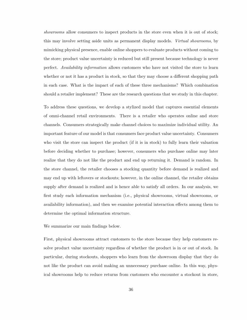
showrooms allow consumers to inspect products in the store even when it is out of stock;
this may involve setting aside units as permanent display models. Virtual showrooms, by
mimicking physical presence, enable online shoppers to evaluate products without coming to
the store; product value uncertainty is reduced but still present because technology is never
perfect. Availability information allows customers who have not visited the store to learn
whether or not it has a product in stock, so that they may choose a different shopping path
in each case. What is the impact of each of these three mechanisms? Which combination
should a retailer implement? These are the research questions that we study in this chapter.
To address these questions, we develop a stylized model that captures essential elements
of omni-channel retail environments. There is a retailer who operates online and store
channels. Consumers strategically make channel choices to maximize individual utility. An
important feature of our model is that consumers face product value uncertainty. Consumers
who visit the store can inspect the product (if it is in stock) to fully learn their valuation
before deciding whether to purchase; however, consumers who purchase online may later
realize that they do not like the product and end up returning it. Demand is random. In
the store channel, the retailer chooses a stocking quantity before demand is realized and
may end up with leftovers or stockouts; however, in the online channel, the retailer obtains
supply after demand is realized and is hence able to satisfy all orders. In our analysis, we
first study each information mechanism (i.e., physical showrooms, virtual showrooms, or
availability information), and then we examine potential interaction effects among them to
determine the optimal information structure.
We summarize our main findings below.
First, physical showrooms attract customers to the store because they help customers re-
solve product value uncertainty regardless of whether the product is in or out of stock. In
particular, during stockouts, shoppers who learn from the showroom display that they do
not like the product can avoid making an unnecessary purchase online. In this way, phys-
ical showrooms help to reduce returns from customers who encounter a stockout in store,
36
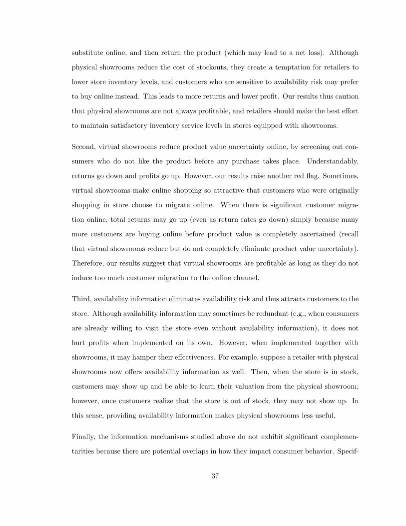
substitute online, and then return the product (which may lead to a net loss). Although
physical showrooms reduce the cost of stockouts, they create a temptation for retailers to
lower store inventory levels, and customers who are sensitive to availability risk may prefer
to buy online instead. This leads to more returns and lower profit. Our results thus caution
that physical showrooms are not always profitable, and retailers should make the best effort
to maintain satisfactory inventory service levels in stores equipped with showrooms.
Second, virtual showrooms reduce product value uncertainty online, by screening out con-
sumers who do not like the product before any purchase takes place. Understandably,
returns go down and profits go up. However, our results raise another red flag. Sometimes,
virtual showrooms make online shopping so attractive that customers who were originally
shopping in store choose to migrate online. When there is significant customer migra-
tion online, total returns may go up (even as return rates go down) simply because many
more customers are buying online before product value is completely ascertained (recall
that virtual showrooms reduce but do not completely eliminate product value uncertainty).
Therefore, our results suggest that virtual showrooms are profitable as long as they do not
induce too much customer migration to the online channel.
Third, availability information eliminates availability risk and thus attracts customers to the
store. Although availability information may sometimes be redundant (e.g., when consumers
are already willing to visit the store even without availability information), it does not
hurt profits when implemented on its own. However, when implemented together with
showrooms, it may hamper their effectiveness. For example, suppose a retailer with physical
showrooms now offers availability information as well. Then, when the store is in stock,
customers may show up and be able to learn their valuation from the physical showroom;
however, once customers realize that the store is out of stock, they may not show up. In
this sense, providing availability information makes physical showrooms less useful.
Finally, the information mechanisms studied above do not exhibit significant complemen-
tarities because there are potential overlaps in how they impact consumer behavior. Specif-
37
ically, physical showrooms and availability information both attract customers to the store,
and both physical and virtual showrooms mitigate product value uncertainty. Given these
overlaps, the optimal information structure often involves choosing one of the three mech-
anisms. For products that are traditionally afflicted with high online return rates, retailers
should establish physical showrooms; however, for products with relatively more manage-
able online return rates, retailers should consider implementing virtual showrooms, and
possibly also provide availability information to maintain the attractiveness of the store
channel.
3.2. Literature Review
Similar to Chapter 2, this chapter also studies the management of online and offline channels.
The traditional literature on channel management focuses on the situation where different
channels are operated by different companies, e.g., Chiang et al. (2003), Cattani et al.
(2006), Chen et al. (2008), and Netessine and Rudi (2006). In contrast to this stream
of work, we focus on an omnichannel environment, where a retailer operates both online
and offline channels in an integrated way (Bell et al., 2014; Brynjolfsson et al., 2013; Rigby,
2011). In this environment, most operations management papers focus on new omnichannel
fulfillment methods. For example, Gallino and Moreno (2014) empirically test the impact
of buy-online-and-pick-up-in-store (BOPS) on a retailer’s sales in both online and offline
channels, while Gao and Su (2016a) (which is based on Chapter 2 of this dissertation)
study the implementation of BOPS and its implications on channel coordination from a
theoretical perspective. Gallino et al. (2016) investigate another widely-used omnichannel
fulfillment option, i.e., ship-to-store, and empirically demonstrate that within a group of
SKUs, the share of sales of bottom-selling items increases. In contrast to these papers, we
focus how to effectively provide information to consumers in the omnichannel environment.
A closely related paper is Bell et al. (2015), which studies the impact of physical showrooms
on consumers’ channel choice. They find that with the introduction of physical showrooms,
customers with a greater need for product information self-select into the physical channel,
38
leading to reduced online returns and increased overall demand. In this chapter, we study
physical showrooms, as well as virtual showrooms and availability information.
There is a large literature devoted to the question of how a firm can induce purchases
from consumers facing product value uncertainty. The most widely studied mechanism
is product returns. Che (1996) and Davis et al. (1995) consider the case where a seller
offers full refunds (or money-back guarantees). Davis et al. (1998) focus on the consumer
hassle costs during the return process, and Moorthy and Srinivasan (1995) show that full
refunds can signal product quality. More recent papers study refund policies in conjunction
with supply chain contracts (Su, 2009), overbooking (Gallego and Sahin, 2010), demand
cannibalization (Akcay et al., 2013), and discount voucher (Gao and Chen, 2015); another
paper by Hsiao and Chen (2012) finds that sellers of low-quality products may have to offer
a refund that exceeds the selling price. The papers above study how returns/refunds can
be used to limit the downside of a bad purchase, but in this chapter, one of our goals is to
reduce the incidence of bad purchases in the first place. To this end, our physical and virtual
showrooms directly reduce product value uncertainty by allowing consumers to experience
products prior to purchase. Ultimately, showrooms and returns policies complement each
other because they serve different functions: while returns policies provide insurance against
consumer loss, showrooms provide product value information.
There is a stream of literature on using product availability as a strategic lever to attract
demand. Being averse to stockouts, consumers may be reluctant to incur the hassle of
going to a store. This practical issue has motivated much work in operations management.
Following the classic paper by Dana and Petruzzi (2001), which extends the newsvendor
model by endogenizing demand as a function of both price and inventory level, many pa-
pers have looked at different strategies to influence consumers’ shopping decisions. Su and
Zhang (2009) show that it is always beneficial to the retailer if he can credibly make an ex
ante quantity commitment. Yin et al. (2009) investigate the impact of two different display
formats, i.e., display-all versus display-one. Allon and Bassamboo (2011) study a situation
39
where a retailer could share unverifiable and nonbinding (i.e., cheap talk) inventory infor-
mation with consumers. Alexandrov and Lariviere (2012) examine the role of reservations
in the context of revenue management. Cachon and Feldman (2015) study dynamic pricing
and find that frequent discounts can attract customers to the store. In contrast to the
previous studies, in this chapter, we consider a different mechanism where a retailer shares
real-time store availability information that reflects the current inventory level available to
each individual customer.
3.3. Base Model
There is a retailer who sells a product through two channels, store and online, at price p.
In the store channel, the retailer faces a newsvendor problem: there is a single inventory
decision q to be made before random demand is realized, so there may eventually be un-
met demand or leftovers in the store. The unit cost of inventory is c, which includes the
production/procurement cost and other store-related costs, e.g., the transportation cost of
shipping the product to store and the inventory holding cost in store. Leftover units have
no value. The online channel is modeled exogenously: for each unit sold online, the retailer
obtains a net profit margin w if it is not returned, and incurs a net loss r otherwise.
The market demand D is random and follows distribution F . A fraction of θ ∈ (0, 1) of
the population has positive value v for the product, and a fraction 1 − θ has zero value.
We refer to the former as “high types,” the latter as “low types,” and the parameter
θ as the “high-type probability.” Customers are homogeneous ex ante: they don’t know
their valuation (or type) beforehand, but θ and v are common knowledge. Customers may
learn their valuations before purchase only if they examine the product in store; otherwise,
customers learn valuations after purchase. In particular, online purchases may be returned,
as described below.
Each consumer makes a choice between shopping online directly or going to the store. If she
chooses to buy online directly, she incurs hassle cost ho (e.g., paying shipping fees or waiting
40
for the product to arrive), and realizes her valuation only after receiving the product. If she
likes the product (i.e., she is high type), then she keeps it and receives payoff v − p− ho; if
she dislikes the product (i.e., she is low type), then she returns it. Returns are costly to both
the retailer and the consumers: each returned unit generates net loss r > 0 to the retailer
and an additional hassle cost hr > 0 to the consumer. We assume that low type consumers
prefer returning the product to keeping it, i.e., hr < p. Therefore, the consumer’s expected
payoff from buying online directly is given by
uo = θ(v − p− ho)− (1− θ)(ho + hr).
On the other hand, if the consumer chooses to go to the store, she has to first incur hassle
cost hs (e.g., traveling to the store or searching for the product in aisles). We stress that
the store hassle cost hs is incurred before customers find and purchase the product in the
store, whereas the online hassle cost ho above is incurred after customers make the purchase
online. Once she is in the store, the customer may encounter two possible outcomes: (1)
If the store has the product in stock, then she can evaluate the product on the spot: a
high type makes a purchase and receives payoff v − p, while a low type leaves without
any purchase and receives payoff 0. (2) If the store is out of stock, she cannot resolve her
value uncertainty in store, but she can buy the product online and receive an expected
payoff uo instead. Let ξ denote the probability that the store is in stock, and let ξ denote
consumers’ beliefs about this probability; throughout this chapter, we use the hat notation ·
to denote beliefs. We assume that customers arrive sequentially to the market, all customer
permutations are equally likely, and customers do not know their order of arrival. As a
result, everyone has the same belief ξ. Then, given belief ξ, each consumer’s payoff from
visiting the store can be expressed as follows:
us(ξ) = −hs + ξθ (v − p) + (1− ξ)uo.
Consumers compare the expected utility from each channel and chooses accordingly. In
41
the spirit of omnichannel choice, i.e., consumers are willing to consider both channels, we
assume v is large enough so that us(1) ≥ 0 and uo ≥ 0.
Next, we consider the retailer’s decision problem. First, the retailer anticipates that a
fraction φ ∈ [0, 1] of customers will visit the store. Then, if total demand is D, the retailer
expects that the number of customers coming to the store will be φD; also, since only
high-type customers will eventually make a purchase in the store, given the store inventory
level q, the retailer expects that the number of store customers who find that the store has
the product in stock is Din (q) = min(φD, qθ
), and the remaining Dout (q) =
(φD − q
θ
)+
will encounter stockouts when they come to the store. Note that even though the inventory
is q, up to qθ customers may examine the product in the store because only a fraction θ of
those customers will buy. Then, the retailer’s profit is as follows:
π (q) = pθEDin (q)− cq (3.1)
+ [wθ − r(1− θ)]EDout (q) (3.2)
+ [wθ − r(1− θ)](1− φ)ED (3.3)
Given the store inventory level q, the newsvendor expected profit from selling the product
in the store channel is shown in the first term (3.1) above. The next two terms respectively
represent profit from customers who switch online after encountering stockouts in the store
and customers who buy online directly. For each unit of online demand, the expected profit
is wθ−r(1−θ), because a fraction (1−θ) of online sales are returned. Again, in the spirit of
omnichannel retailing, we assume wθ− r(1− θ) > 0 so that the retailer is willing to operate
both channels. Finally, the retailer chooses inventory level q to maximize expected profit.
To study the strategic interaction between the retailer and the consumers, we shall use the
rational expectations (RE) equilibrium concept, as what we did in Chapter 2. One impor-
tant feature of a RE equilibrium is that beliefs must be consistent with actual outcomes. In
other words, the retailer’s belief φ must coincide with the true proportion φ of consumers
42
choosing the store channel, and consumers’ beliefs over in-store inventory availability ξ must
agree with the actual in-stock probability corresponding to the retailer’s chosen quantity q.
This probability is given by A(q) = Emin(φD, qθ )/E(φD), where φ > 0, using the derivation
from Deneckere and Peck (1995) and Dana (2001). Then, we have the following definition
for a RE equilibrium. Henceforth, we refer to the RE equilibrium as “equilibrium” for
brevity.
Definition 3. A RE equilibrium (φ, q, ξ, φ) satisfies the following:
i Given ξ, if us(ξ) > uo, then φ = 1; otherwise φ = 0;
ii. Given φ, q = arg maxq π(q).
iii. ξ = A(q).
iv. φ = φ.
Conditions (i) and (ii) state that under beliefs ξ and φ, the consumers and the retailer are
choosing the optimal decisions. Conditions (iii) and (iv) are the consistency conditions.
First, note that there is always a nonparticipatory equilibrium (0, 0, 0, 0). If the retailer
expects that no one will come to the store, he will stock nothing there, i.e., q = 0; If
consumers believe there is no inventory in the store, they will not come, i.e., φ = 0. In the
end, we have a self-fulfilling prophecy and beliefs are trivially consistent with the actual
outcome.
Is there any participatory equilibrium where consumers are willing to visit the store and the
retailer has stock in the store as well (i.e., φ = 1 and q > 0)? When such an equilibrium
exists, it Pareto-dominates the nonparticipatory equilibrium. The reasoning is as follows.
In the participatory equilibrium, customers choose to visit the store rather than buying
online directly (as what they would do in the nonparticipatory equilibrium), so they must
be better off in the former. Similarly, the retailer prefers to stock q > 0 in the participatory
equilibrium rather than choosing q = 0 (which leads customers to buy online and yields
43
the same profit as the nonparticipatory equilibrium), so the retailer must also be better
off in the participatory equilibrium. In this chapter, we shall adopt the Pareto dominance
equilibrium selection rule. The following proposition gives the equilibrium result; we use
the superscript (·◦) to denote the equilibrium outcome for this base scenario.
Proposition 11. There exists a threshold ψ◦ ∈ [0, 1] such that
• if θ < ψ◦, then consumers visit the store and q◦ = θF−1
(c
p−w+r 1−θθ
)> 0;
• if θ ≥ ψ◦, then consumers buy online directly and q◦ = 0.
Proposition 11 shows that consumers come to the store only if the high-type probability
is low (i.e., θ < ψ◦) and they recognize the need to touch and feel the product before
making a purchase. In this case, the retailer prepares a positive amount of inventory in the
store to accommodate consumer demand. To the retailer, the overage cost is simply the
inventory cost c and the underage cost is given by p− c− w + r 1−θθ . The latter expression
is the combination of two effects. First, each unit of underage is a lost opportunity of
selling to a high type, who buys online instead, leading to a difference in profit margin of
p− c−w. Second, each unit of underage is also a lost opportunity for customers to realize
their valuations (by inspecting that unit of inventory); corresponding to one high type who
could have bought this unit are 1−θθ low types who could have realized their low valuations
and thus avoided the return cost r. Thus, as the online return cost r increases, the retailer
holds more inventory, purely for informational purposes.
3.4. Physical Showrooms
Previously, in the base model, consumers can evaluate the product in the store only if it is
in stock. Now suppose that there is a physical showroom in the store, so that consumers
can always inspect the product, even when it is out of stock. In this section, we study the
equilibrium outcomes and profit implications of adding such a physical showroom.
As before, we start by considering the consumer’s choice between shopping online and
44
in store. The consumer’s payoff from visiting the store is us(ξ) = −hs + ξθ (v − p) +
(1− ξ)θ (v − p− ho), given her belief about store inventory availability ξ. Note that the
first two parts of us remain the same as in the base model. The only change occurs in the
third term: when the consumer encounters stockouts in store, she is still able to realize her
valuation from the physical showroom; she chooses to purchase online and receives payoff
v − p − ho only if she is of high type. The consumer’s payoff from buying online directly,
on the other hand, remains unchanged as uo = θ(v − p− ho)− (1− θ)(ho + hr).
The retailer has a belief φ about the fraction of consumers who would visit the store. Given
this belief, the retailer’s profit is as follows.
π (q) = pθEDin (q)− cq (3.4)
+ wθEDout (q) (3.5)
+ [wθ − r(1− θ)](1− φ)ED (3.6)
Comparing this to the profit function in the base model, we note that the only difference
occurs in the term (3.5): this is because the physical showroom allows low types who
encounter stockouts to learn their types and thus avoid the trouble of buying online and then
returning. However, the two profit functions become identical when r = 0. Nevertheless, the
retailer may still obtain different profits in equilibrium because consumer channel choices
may change after the implementation of physical showrooms (i.e., φ in equilibrium may be
different), as shown below.
Similar to the analysis of the base model, we apply the notion of RE equilibrium to describe
the market outcome. We use superscript ·p to denote physical showrooms.
Proposition 12. With physical showrooms, there exists a threshold ψp ∈ [0, 1] such that
• if θ < ψp, then consumers visit the store and qp = θF−1(
cp−w
)≥ 0;
• if θ ≥ ψp, then consumers buy online directly and qp = 0.
45
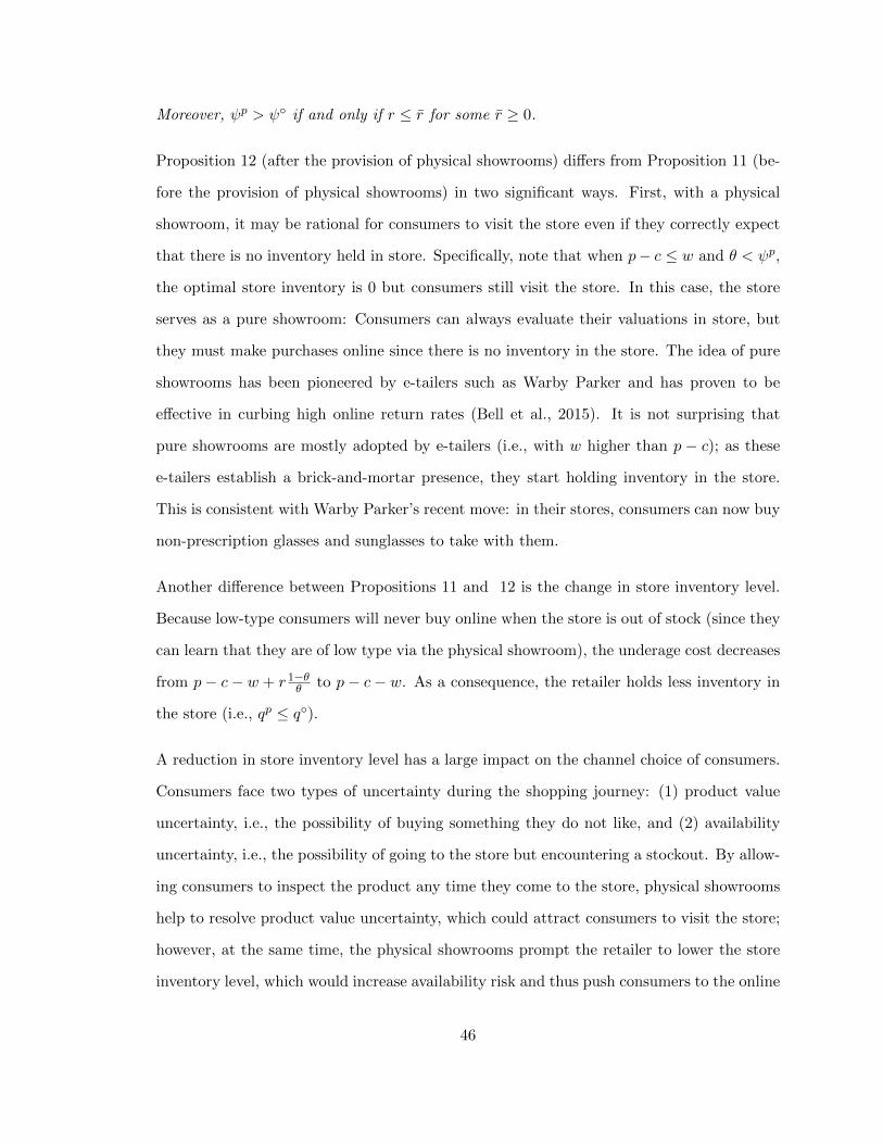
Moreover, ψp > ψ◦ if and only if r ≤ r for some r ≥ 0.
Proposition 12 (after the provision of physical showrooms) differs from Proposition 11 (be-
fore the provision of physical showrooms) in two significant ways. First, with a physical
showroom, it may be rational for consumers to visit the store even if they correctly expect
that there is no inventory held in store. Specifically, note that when p− c ≤ w and θ < ψp,
the optimal store inventory is 0 but consumers still visit the store. In this case, the store
serves as a pure showroom: Consumers can always evaluate their valuations in store, but
they must make purchases online since there is no inventory in the store. The idea of pure
showrooms has been pioneered by e-tailers such as Warby Parker and has proven to be
effective in curbing high online return rates (Bell et al., 2015). It is not surprising that
pure showrooms are mostly adopted by e-tailers (i.e., with w higher than p − c); as these
e-tailers establish a brick-and-mortar presence, they start holding inventory in the store.
This is consistent with Warby Parker’s recent move: in their stores, consumers can now buy
non-prescription glasses and sunglasses to take with them.
Another difference between Propositions 11 and 12 is the change in store inventory level.
Because low-type consumers will never buy online when the store is out of stock (since they
can learn that they are of low type via the physical showroom), the underage cost decreases
from p− c− w + r 1−θθ to p− c− w. As a consequence, the retailer holds less inventory in
the store (i.e., qp ≤ q◦).
A reduction in store inventory level has a large impact on the channel choice of consumers.
Consumers face two types of uncertainty during the shopping journey: (1) product value
uncertainty, i.e., the possibility of buying something they do not like, and (2) availability
uncertainty, i.e., the possibility of going to the store but encountering a stockout. By allow-
ing consumers to inspect the product any time they come to the store, physical showrooms
help to resolve product value uncertainty, which could attract consumers to visit the store;
however, at the same time, the physical showrooms prompt the retailer to lower the store
inventory level, which would increase availability risk and thus push consumers to the online
46
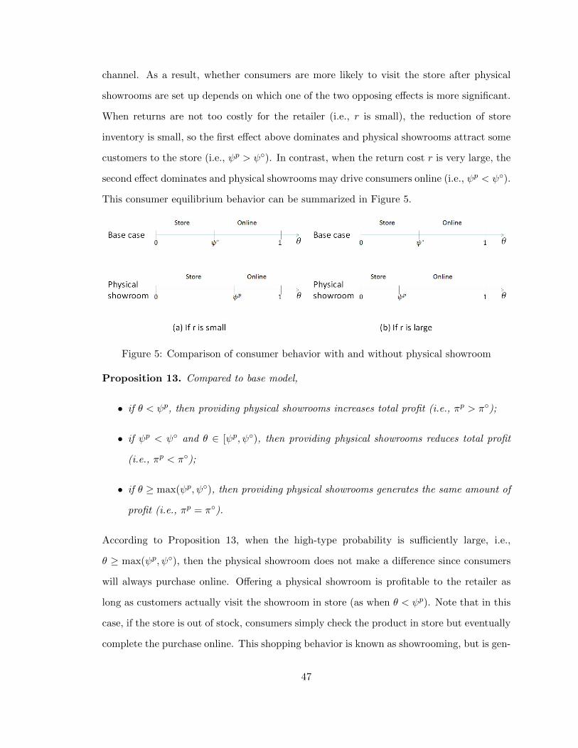
channel. As a result, whether consumers are more likely to visit the store after physical
showrooms are set up depends on which one of the two opposing effects is more significant.
When returns are not too costly for the retailer (i.e., r is small), the reduction of store
inventory is small, so the first effect above dominates and physical showrooms attract some
customers to the store (i.e., ψp > ψ◦). In contrast, when the return cost r is very large, the
second effect dominates and physical showrooms may drive consumers online (i.e., ψp < ψ◦).
This consumer equilibrium behavior can be summarized in Figure 5.
Figure 5: Comparison of consumer behavior with and without physical showroom
Proposition 13. Compared to base model,
• if θ < ψp, then providing physical showrooms increases total profit (i.e., πp > π◦);
• if ψp < ψ◦ and θ ∈ [ψp, ψ◦), then providing physical showrooms reduces total profit
(i.e., πp < π◦);
• if θ ≥ max(ψp, ψ◦), then providing physical showrooms generates the same amount of
profit (i.e., πp = π◦).
According to Proposition 13, when the high-type probability is sufficiently large, i.e.,
θ ≥ max(ψp, ψ◦), then the physical showroom does not make a difference since consumers
will always purchase online. Offering a physical showroom is profitable to the retailer as
long as customers actually visit the showroom in store (as when θ < ψp). Note that in this
case, if the store is out of stock, consumers simply check the product in store but eventually
complete the purchase online. This shopping behavior is known as showrooming, but is gen-
47
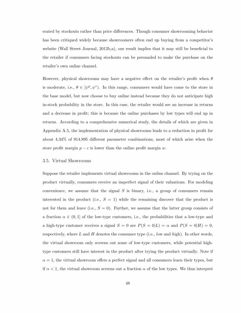
erated by stockouts rather than price differences. Though consumer showrooming behavior
has been critiqued widely because showroomers often end up buying from a competitor’s
website (Wall Street Journal, 2012b,a), our result implies that it may still be beneficial to
the retailer if consumers facing stockouts can be persuaded to make the purchase on the
retailer’s own online channel.
However, physical showrooms may have a negative effect on the retailer’s profit when θ
is moderate, i.e., θ ∈ [ψp, ψ◦). In this range, consumers would have come to the store in
the base model, but now choose to buy online instead because they do not anticipate high
in-stock probability in the store. In this case, the retailer would see an increase in returns
and a decrease in profit; this is because the online purchases by low types will end up in
returns. According to a comprehensive numerical study, the details of which are given in
Appendix A.5, the implementation of physical showrooms leads to a reduction in profit for
about 4.34% of 914,895 different parameter combinations, most of which arise when the
store profit margin p− c is lower than the online profit margin w.
3.5. Virtual Showrooms
Suppose the retailer implements virtual showrooms in the online channel. By trying on the
product virtually, consumers receive an imperfect signal of their valuations. For modeling
convenience, we assume that the signal S is binary, i.e., a group of consumers remain
interested in the product (i.e., S = 1) while the remaining discover that the product is
not for them and leave (i.e., S = 0). Further, we assume that the latter group consists of
a fraction α ∈ (0, 1] of the low-type customers, i.e., the probabilities that a low-type and
a high-type customer receives a signal S = 0 are P (S = 0|L) = α and P (S = 0|H) = 0,
respectively, where L and H denotes the consumer type (i.e., low and high). In other words,
the virtual showroom only screens out some of low-type customers, while potential high-
type customers still have interest in the product after trying the product virtually. Note if
α = 1, the virtual showroom offers a perfect signal and all consumers learn their types, but
if α < 1, the virtual showroom screens out a fraction α of the low types. We thus interpret
48
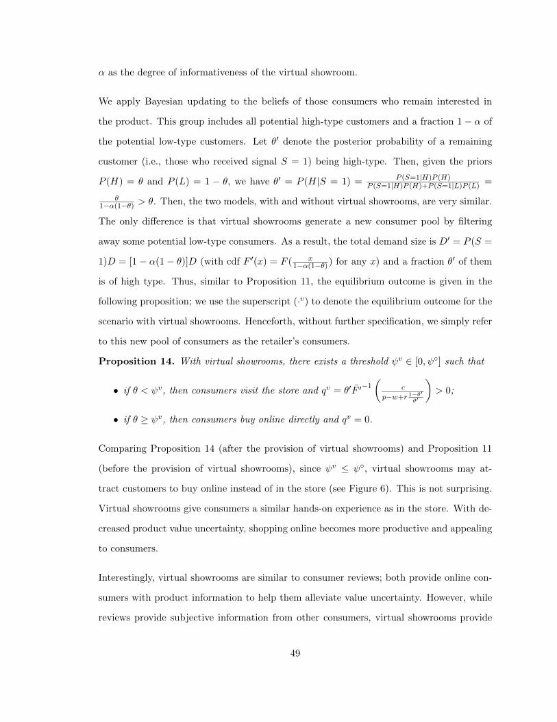
α as the degree of informativeness of the virtual showroom.
We apply Bayesian updating to the beliefs of those consumers who remain interested in
the product. This group includes all potential high-type customers and a fraction 1− α of
the potential low-type customers. Let θ′ denote the posterior probability of a remaining
customer (i.e., those who received signal S = 1) being high-type. Then, given the priors
P (H) = θ and P (L) = 1 − θ, we have θ′ = P (H|S = 1) = P (S=1|H)P (H)P (S=1|H)P (H)+P (S=1|L)P (L) =
θ1−α(1−θ) > θ. Then, the two models, with and without virtual showrooms, are very similar.
The only difference is that virtual showrooms generate a new consumer pool by filtering
away some potential low-type consumers. As a result, the total demand size is D′ = P (S =
1)D = [1− α(1− θ)]D (with cdf F ′(x) = F ( x1−α(1−θ)) for any x) and a fraction θ′ of them
is of high type. Thus, similar to Proposition 11, the equilibrium outcome is given in the
following proposition; we use the superscript (·v) to denote the equilibrium outcome for the
scenario with virtual showrooms. Henceforth, without further specification, we simply refer
to this new pool of consumers as the retailer’s consumers.
Proposition 14. With virtual showrooms, there exists a threshold ψv ∈ [0, ψ◦] such that
• if θ < ψv, then consumers visit the store and qv = θ′F ′−1(
c
p−w+r 1−θ′θ′
)> 0;
• if θ ≥ ψv, then consumers buy online directly and qv = 0.
Comparing Proposition 14 (after the provision of virtual showrooms) and Proposition 11
(before the provision of virtual showrooms), since ψv ≤ ψ◦, virtual showrooms may at-
tract customers to buy online instead of in the store (see Figure 6). This is not surprising.
Virtual showrooms give consumers a similar hands-on experience as in the store. With de-
creased product value uncertainty, shopping online becomes more productive and appealing
to consumers.
Interestingly, virtual showrooms are similar to consumer reviews; both provide online con-
sumers with product information to help them alleviate value uncertainty. However, while
reviews provide subjective information from other consumers, virtual showrooms provide
49
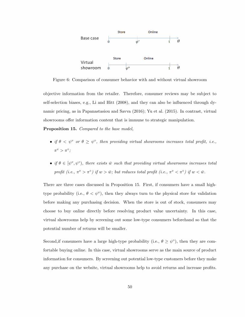
Figure 6: Comparison of consumer behavior with and without virtual showroom
objective information from the retailer. Therefore, consumer reviews may be subject to
self-selection biases, e.g., Li and Hitt (2008), and they can also be influenced through dy-
namic pricing, as in Papanastasiou and Savva (2016); Yu et al. (2015). In contrast, virtual
showrooms offer information content that is immune to strategic manipulation.
Proposition 15. Compared to the base model,
• if θ < ψv or θ ≥ ψ◦, then providing virtual showrooms increases total profit, i.e.,
πv > π◦;
• if θ ∈ [ψv, ψ◦), there exists w such that providing virtual showrooms increases total
profit (i.e., πv > π◦) if w > w; but reduces total profit (i.e., πv < π◦) if w < w.
There are three cases discussed in Proposition 15. First, if consumers have a small high-
type probability (i.e., θ < ψv), then they always turn to the physical store for validation
before making any purchasing decision. When the store is out of stock, consumers may
choose to buy online directly before resolving product value uncertainty. In this case,
virtual showrooms help by screening out some low-type consumers beforehand so that the
potential number of returns will be smaller.
Second,if consumers have a large high-type probability (i.e., θ ≥ ψ◦), then they are com-
fortable buying online. In this case, virtual showrooms serve as the main source of product
information for consumers. By screening out potential low-type customers before they make
any purchase on the website, virtual showrooms help to avoid returns and increase profits.
50
However, when θ ∈ [ψv, ψ◦), implementing virtual showrooms may backfire. In this case,
consumers originally visit the store in the base model, but virtual showrooms attract them
to buy online instead. Although the online return rate decreases from 1 − θ (without
virtual showroom) to 1 − θ′ (with virtual showroom), total returns may increase. This is
because more people now choose to buy online, including low types who are destined to
return their purchases. The resulting increase in returns will drive down total profit. Unless
the online profit margin is high enough, customer migration from store to online will be
unprofitable for the retailer. This result offers a possible explanation for fashion retailer
H&M’s decision to remove their virtual showroom (called the Dressing Room) from their
website even though it has been popular among consumers (H&M, 2010). Our result also
suggests that retailers should be cautious when looking at online return rates and should
not neglect the total number of returns as an informative companion metric. According
to a comprehensive numerical study, the details of which are given in Appendix A.5, the
implementation of virtual showrooms hurts profits for about 4.58% of 914,895 different
parameter combinations, most of which arise when the online profit margin w is lower than
the store profit margin p− c.
3.6. Availability Information
Suppose the retailer provides availability information on its website, so that consumers
are able to check real-time store inventory status. With such information, the sequence of
consumer arrivals matter: consumers who arrive early will see that the store has inventory
in stock, but consumers who arrive late will encounter stockouts. In the former case, the
consumer can go to the store and receive an expected payoff of us,in = −hs + θ(v − p)
because she will certainly obtain the product if she realizes high valuation. In the latter
case, the consumer will receive nothing from visiting the store and thus will choose to buy
online instead. In practice, some retailers may also reveal the number of units in inventory
as part of the availability information. This does not change consumers’ shopping behavior
in our model, since consumers care only about whether the store is in stock or not when
51
they arrive in the market.
Each consumer chooses between shopping online directly or going to the store, given the
current store inventory availability status. Let φin denote the fraction of customers visiting
the store when it is in stock. As before, only high-type consumers will absorb store inventory
when they come to the store. Then, the expected number of customers who see that the
store is in stock is Din (q) = min(D, q
θφin
), and the remaining Dout (q) =
(D − q
θφin
)+will
find that the store is already out of stock when they check availability online. Note that the
expressions for Din(q) and Dout(q) are slightly different from before because all consumers,
whether or not they choose to come to the store, will receive availability information. Thus,
the retailer’s profit function is as follows:
π (q) = pθφinEDin (q)− cq (3.7)
+ [wθ − r(1− θ)] (1− φin)EDin (q) (3.8)
+ [wθ − r(1− θ)]EDout (q) (3.9)
The first two parts of the profit function correspond to the case when the store is in stock:
(3.7) is the newsvendor profit from the store, and (3.8) is the profit from those who buy
online directly. The last part (3.9) corresponds to the case when the store is out of stock
and all consumers buy online.
We use superscript (·a) to denote the market outcome with availability information, which
is given in the following proposition.
Proposition 16. With availability information, there exists a threshold ψa ∈ [ψ◦, 1] such
that the market outcome is given as follows:
• If θ < ψa, then consumers visit store if store is in stock, and buy online directly if
store is out of stock; qa = θF−1
(c
p−w+r 1−θθ
)> 0
• If θ ≥ ψa, then consumers always buy online directly; qa = 0.
52
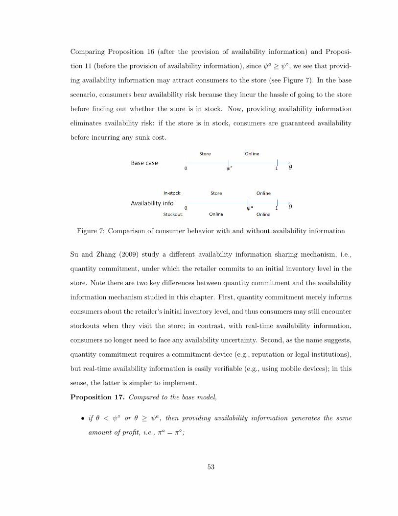
Comparing Proposition 16 (after the provision of availability information) and Proposi-
tion 11 (before the provision of availability information), since ψa ≥ ψ◦, we see that provid-
ing availability information may attract consumers to the store (see Figure 7). In the base
scenario, consumers bear availability risk because they incur the hassle of going to the store
before finding out whether the store is in stock. Now, providing availability information
eliminates availability risk: if the store is in stock, consumers are guaranteed availability
before incurring any sunk cost.
Figure 7: Comparison of consumer behavior with and without availability information
Su and Zhang (2009) study a different availability information sharing mechanism, i.e.,
quantity commitment, under which the retailer commits to an initial inventory level in the
store. Note there are two key differences between quantity commitment and the availability
information mechanism studied in this chapter. First, quantity commitment merely informs
consumers about the retailer’s initial inventory level, and thus consumers may still encounter
stockouts when they visit the store; in contrast, with real-time availability information,
consumers no longer need to face any availability uncertainty. Second, as the name suggests,
quantity commitment requires a commitment device (e.g., reputation or legal institutions),
but real-time availability information is easily verifiable (e.g., using mobile devices); in this
sense, the latter is simpler to implement.
Proposition 17. Compared to the base model,
• if θ < ψ◦ or θ ≥ ψa, then providing availability information generates the same
amount of profit, i.e., πa = π◦;
53
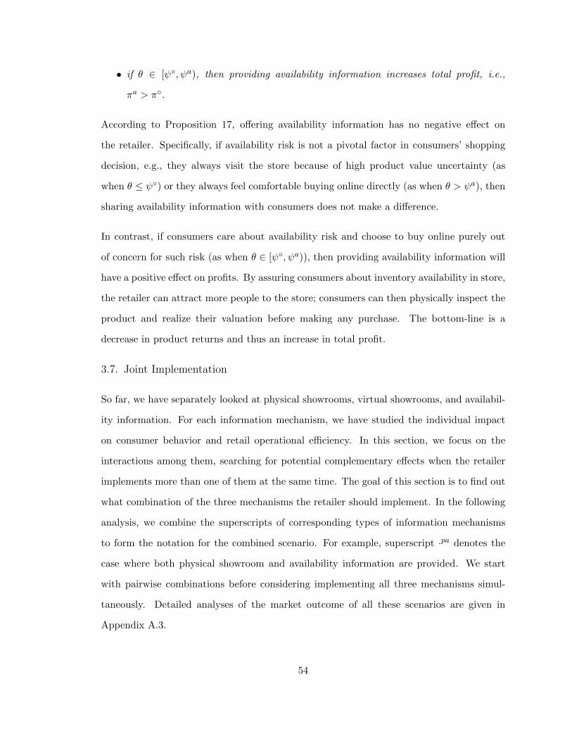
• if θ ∈ [ψ◦, ψa), then providing availability information increases total profit, i.e.,
πa > π◦.
According to Proposition 17, offering availability information has no negative effect on
the retailer. Specifically, if availability risk is not a pivotal factor in consumers’ shopping
decision, e.g., they always visit the store because of high product value uncertainty (as
when θ ≤ ψ◦) or they always feel comfortable buying online directly (as when θ > ψa), then
sharing availability information with consumers does not make a difference.
In contrast, if consumers care about availability risk and choose to buy online purely out
of concern for such risk (as when θ ∈ [ψ◦, ψa)), then providing availability information will
have a positive effect on profits. By assuring consumers about inventory availability in store,
the retailer can attract more people to the store; consumers can then physically inspect the
product and realize their valuation before making any purchase. The bottom-line is a
decrease in product returns and thus an increase in total profit.
3.7. Joint Implementation
So far, we have separately looked at physical showrooms, virtual showrooms, and availabil-
ity information. For each information mechanism, we have studied the individual impact
on consumer behavior and retail operational efficiency. In this section, we focus on the
interactions among them, searching for potential complementary effects when the retailer
implements more than one of them at the same time. The goal of this section is to find out
what combination of the three mechanisms the retailer should implement. In the following
analysis, we combine the superscripts of corresponding types of information mechanisms
to form the notation for the combined scenario. For example, superscript ·pa denotes the
case where both physical showroom and availability information are provided. We start
with pairwise combinations before considering implementing all three mechanisms simul-
taneously. Detailed analyses of the market outcome of all these scenarios are given in
Appendix A.3.
54
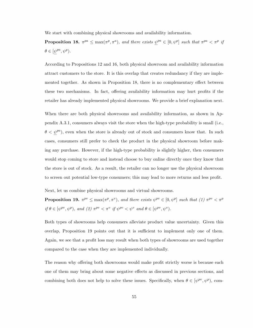
We start with combining physical showrooms and availability information.
Proposition 18. πpa ≤ max(πp, πa), and there exists ψpa ∈ [0, ψp] such that πpa < πp if
θ ∈ [ψpa, ψp).
According to Propositions 12 and 16, both physical showroom and availability information
attract customers to the store. It is this overlap that creates redundancy if they are imple-
mented together. As shown in Proposition 18, there is no complementary effect between
these two mechanisms. In fact, offering availability information may hurt profits if the
retailer has already implemented physical showrooms. We provide a brief explanation next.
When there are both physical showrooms and availability information, as shown in Ap-
pendix A.3.1, consumers always visit the store when the high-type probability is small (i.e.,
θ < ψpa), even when the store is already out of stock and consumers know that. In such
cases, consumers still prefer to check the product in the physical showroom before mak-
ing any purchase. However, if the high-type probability is slightly higher, then consumers
would stop coming to store and instead choose to buy online directly once they know that
the store is out of stock. As a result, the retailer can no longer use the physical showroom
to screen out potential low-type consumers; this may lead to more returns and less profit.
Next, let us combine physical showrooms and virtual showrooms.
Proposition 19. πpv ≤ max(πp, πv), and there exists ψpv ∈ [0, ψp] such that (1) πpv < πp
if θ ∈ [ψpv, ψp), and (2) πpv < πv if ψpv < ψv and θ ∈ [ψpv, ψv).
Both types of showrooms help consumers alleviate product value uncertainty. Given this
overlap, Proposition 19 points out that it is sufficient to implement only one of them.
Again, we see that a profit loss may result when both types of showrooms are used together
compared to the case when they are implemented individually.
The reason why offering both showrooms would make profit strictly worse is because each
one of them may bring about some negative effects as discussed in previous sections, and
combining both does not help to solve these issues. Specifically, when θ ∈ [ψpv, ψp), com-
55
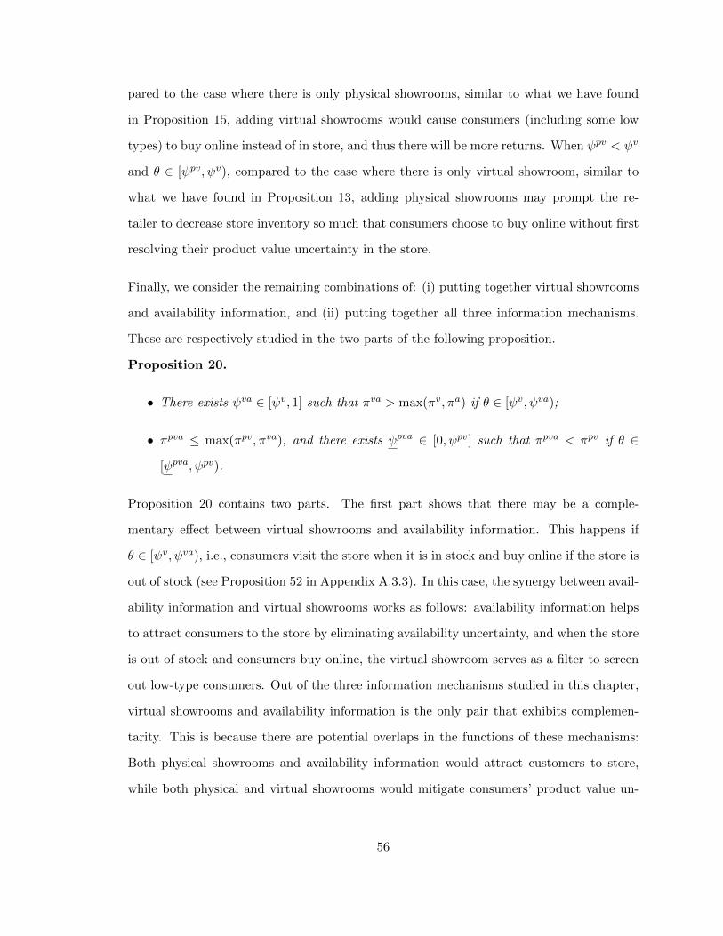
pared to the case where there is only physical showrooms, similar to what we have found
in Proposition 15, adding virtual showrooms would cause consumers (including some low
types) to buy online instead of in store, and thus there will be more returns. When ψpv < ψv
and θ ∈ [ψpv, ψv), compared to the case where there is only virtual showroom, similar to
what we have found in Proposition 13, adding physical showrooms may prompt the re-
tailer to decrease store inventory so much that consumers choose to buy online without first
resolving their product value uncertainty in the store.
Finally, we consider the remaining combinations of: (i) putting together virtual showrooms
and availability information, and (ii) putting together all three information mechanisms.
These are respectively studied in the two parts of the following proposition.
Proposition 20.
• There exists ψva ∈ [ψv, 1] such that πva > max(πv, πa) if θ ∈ [ψv, ψva);
• πpva ≤ max(πpv, πva), and there exists ψpva ∈ [0, ψpv] such that πpva < πpv if θ ∈
[ψpva, ψpv).
Proposition 20 contains two parts. The first part shows that there may be a comple-
mentary effect between virtual showrooms and availability information. This happens if
θ ∈ [ψv, ψva), i.e., consumers visit the store when it is in stock and buy online if the store is
out of stock (see Proposition 52 in Appendix A.3.3). In this case, the synergy between avail-
ability information and virtual showrooms works as follows: availability information helps
to attract consumers to the store by eliminating availability uncertainty, and when the store
is out of stock and consumers buy online, the virtual showroom serves as a filter to screen
out low-type consumers. Out of the three information mechanisms studied in this chapter,
virtual showrooms and availability information is the only pair that exhibits complemen-
tarity. This is because there are potential overlaps in the functions of these mechanisms:
Both physical showrooms and availability information would attract customers to store,
while both physical and virtual showrooms would mitigate consumers’ product value un-
56
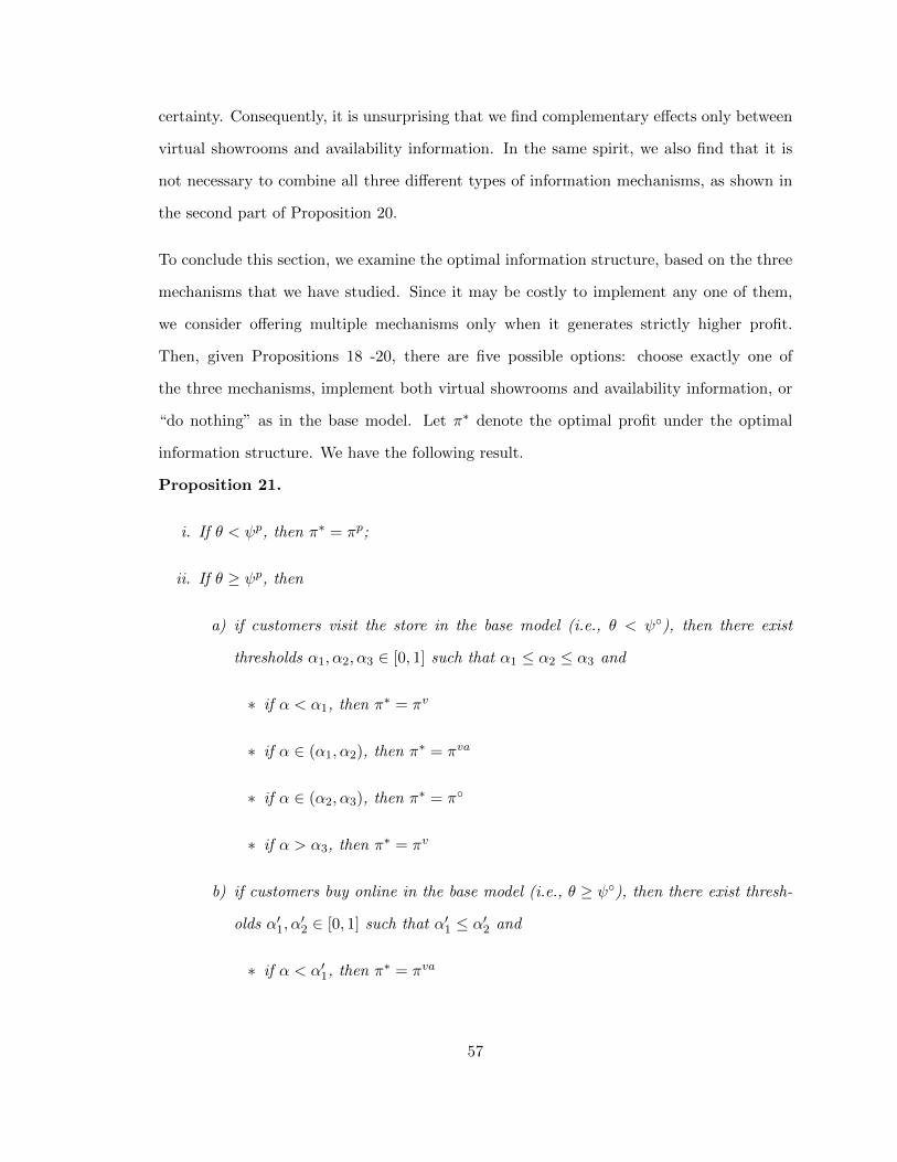
certainty. Consequently, it is unsurprising that we find complementary effects only between
virtual showrooms and availability information. In the same spirit, we also find that it is
not necessary to combine all three different types of information mechanisms, as shown in
the second part of Proposition 20.
To conclude this section, we examine the optimal information structure, based on the three
mechanisms that we have studied. Since it may be costly to implement any one of them,
we consider offering multiple mechanisms only when it generates strictly higher profit.
Then, given Propositions 18 -20, there are five possible options: choose exactly one of
the three mechanisms, implement both virtual showrooms and availability information, or
“do nothing” as in the base model. Let π∗ denote the optimal profit under the optimal
information structure. We have the following result.
Proposition 21.
i. If θ < ψp, then π∗ = πp;
ii. If θ ≥ ψp, then
a) if customers visit the store in the base model (i.e., θ < ψ◦), then there exist
thresholds α1, α2, α3 ∈ [0, 1] such that α1 ≤ α2 ≤ α3 and
∗ if α < α1, then π∗ = πv
∗ if α ∈ (α1, α2), then π∗ = πva
∗ if α ∈ (α2, α3), then π∗ = π◦
∗ if α > α3, then π∗ = πv
b) if customers buy online in the base model (i.e., θ ≥ ψ◦), then there exist thresh-
olds α′1, α′2 ∈ [0, 1] such that α′1 ≤ α′2 and
∗ if α < α′1, then π∗ = πva
57
∗ if α ∈ (α′1, α′2), then π∗ = πa
∗ if α > α′2, then π∗ = πv
Proposition 21 suggests that the main driver behind the optimal information mechanism is
the parameter θ, i.e., the high-type probability. Part (i) of the proposition shows that when
θ is low (i.e., θ < ψp), it is optimal to provide only physical showrooms; part (ii) shows
that when θ is high (i.e., θ ≥ ψp), virtual showrooms or/and availability information work
better. A reasonable proxy for the θ parameter is the online return rate, since products with
a smaller high-type probability θ are more likely to be returned. Therefore, Proposition 21(i)
suggests that for products that are traditionally afflicted with high online return rates (e.g.,
fashion apparel and accessories), physical showrooms should be implemented to attract
customers into stores to touch and feel the product before making a purchase. Our analysis
advocates physical showrooms rather than virtual showrooms, which tend to be a more
intuitive choice for retailers plagued by online returns. Our finding is also consistent with
the recent move by many fashion retailers’ (e.g., Bonobos and Warby Parker’s) to build
more physical showrooms (New York Times, 2014; Wall Street Journal, 2014b).
Next, for products with relatively more manageable online return rates, such as home goods
and electronics (Laseter and Rabinovich, 2011, pg.118), Proposition 21(ii) describes the
optimal information mechanism. Depending on whether customers visit the store or buy
online directly in the base model (i.e., without any information mechanism), the baseline
scenarios are different and our results are separately reported in parts (ii)(a) and (ii)(b).
In both cases, our results suggest that the retailer should consider implementing virtual
showrooms to provide product value information to consumers, and possibly also provide
availability information to maintain the attractiveness of the store channel. In part (ii)(a),
we also find that when customers visit the store in the base model, it may be optimal to
not implement any additional information mechanism at all.
Proposition 21 also demonstrates the importance of the α parameter, i.e., the informative-
58
ness of the virtual showroom. Some implementations of virtual showrooms involve rela-
tively rudimentary functions (e.g., picture upload), while others use more advanced virtual
reality technologies (e.g., 3D technology) which offer online shoppers a more vivid try-on
experience. As virtual showrooms become more informative (i.e., as α increases), Proposi-
tion 21(ii) shows that it is possible for them to become less attractive. Specifically, in both
parts (a) and (b), virtual showrooms are a part of the optimal information mechanism only
when α is either sufficiently large or sufficiently small. In other words, attempts to enhance
the informativeness of virtual showrooms, if not significant, may reduce profits. The reason
is as follows: unless the virtual showroom becomes very effective in screening out low-type
customers, it may simply end up attracting online transactions and thus increasing online
returns.
3.8. Extensions
3.8.1. Endogenous Online Channel
In our original model, we have assumed that the online channel is exogenous; specifically,
there is always enough inventory to satisfy online demand. We can extend our basic model
to include an endogenous online channel as follows. Suppose the retailer has a one-time
ordering opportunity to prepare the inventory level qs and qo in the store and online channel.
The unit inventory costs in the store and online channels are cs and co, respectively. The
product price p is still the same across both channels. Then, for each unit of product sold
online, if it is not returned, the retailer earns the revenue p; if it is returned, the retailer
incurs a net cost k. When the store is out of stock, consumers may switch back to the
retailer’s online channel as before. When the online channel is out of stock, those who are
willing to buy online will leave for other websites to buy the product at the same price.
In many companies (e.g., Bonobos and Warby Parker), store employees are trained and
equipped with digital devices to help store customers order online. However, when customers
are shopping online at home, it is hard for a firm to persuade customers to come to store
when online is out of stock. Our model setup is to capture this difference. Appendix A.4.1
59
presents a detailed analysis of this model. We find that the drivers behind consumer channel
choice and the effects of the three information mechanisms remain unchanged.
3.8.2. Continuous Valuations
Our analysis has assumed that consumer valuation can take on only two values, either v or
0. As a result, there are only two types of customer in the market, i.e., high types (who
like the product) and low types (who don’t). Our model can be extended to a more general
case. Suppose consumer valuation V follows a continuous distribution G. Similar as our
basic model, consumers are homogeneous ex ante; they know the distribution G but not
their individual valuation beforehand.
Consumers who buy online directly will realize their valuations after receiving the delivery,
and there are three possible outcomes. Consumers with V > p will find that they like
the product and thus keep it, and consumers with V < p − hr will find that they do not
like the product and thus return it. These two types of behavior correspond to the high
type and low type in the basic model. Finally, we have a third possibility: consumers with
V ∈ (p − hr, p) will find that they do not like the product (since V − p < 0) but they still
choose to keep it rather than going through the hassles of returning it back to the retailer
(since −hr < V − p).
When there is a virtual showroom, similar as in the basic model, we assume that it helps
to screen out some “low-type” customers in the online channel. Specifically, the signal
consumers receive after checking with the virtual showroom is binary: those with valuation
V < v will realize that their valuation is low and therefore leave the market without any
purchase, while those with valuation V ≥ v will realize that their valuation is greater than
v and update their belief about the valuation distribution to G′ such that ∀v ≥ v, G′(v) =
G(v)−G(v)1−G(v) , where the threshold v ≤ p−hr. With some “low-type” customers being screened
out, the total number of customers left in the market is D′ = [1−G(v)]D. Then, we obtain
a new customer pool with total demand size D′ and valuation distribution G′. A detailed
60
analysis of this model extension is given in Appendix A.4.2, from which we find that our
main insights remain valid.
3.8.3. Informed and Uninformed Consumers
So far, we have assumed that consumers are homogeneous at the beginning of their shopping
journey, although they may have different realized valuations ex post. We can extend our
basic model to incorporate ex ante heterogeneity in the consumer population. Specifically,
suppose that a fraction λ of the customers are informed, i.e., they know that they are
of high type (i.e., with valuation v) right from the beginning. The remaining fraction
1 − λ of customers are uninformed as before, i.e., they do not know their types but they
know the high-type probability θ. As a result, only uninformed customers will react to the
implementation of physical/virtual showrooms, since informed customers do not need any
product value information.
Appendix A.4.3 presents a detailed analysis of our extended model, which shows that most
of our key insights continue to hold. However, there is a slight difference: specifically, we
find that the retailer may sometimes wish to offer both physical showrooms and availability
information (because the former caters to uninformed customers while the latter caters to
informed customers). Nevertheless, we continue to find that physical and virtual showrooms
do not exhibit any complementary effects.
3.8.4. Heterogeneous Valuations
In our analysis, we have assumed that customers have the same valuation v if they find
they like the product. Our model can also be extended to the case where consumers have
heterogeneous valuations. Suppose there are two types of customers and a fraction θ of the
first (second) type customers has value v1 (v2), and a fraction 1− θ has zero value. Then,
as long as both types of customers are willing to consider both channels, i.e., usi(1) ≥ 0 and
uoi ≥ 0, i = 1, 2, all of our previous results continue to hold. The reason is as follows: Each
consumer’s channel choice (which is determined by the sign of usi − uoi) is independent
61
of their valuation. Also, because customers pay the same price and they have the same
probability 1 − θ of returning the product, the retailer obtains the same expected profit
from each type of customers. In other words, from the retailer’s perspective, the two types
of customer are the same.
3.9. Conclusion
Consumers are no longer dedicated to one particular channel. Their shopping journey has
become omnichannel; they strategically switch channels to best suit their personal conve-
nience when evaluating and purchasing products. In response, more and more retailers are
starting to transition from the traditional channel-specific management style to omnichan-
nel operations, where different channels are integrated in a seamless way. In this chapter, we
studied three omnichannel information mechanisms, i.e., physical showrooms, virtual show-
rooms, and availability information, which have been recently experimented and adopted
by an increasing number of retailers.
The implementation of any omnichannel strategy is not easy. For example, to set up phys-
ical showrooms, a retailer may need to restructure its stores; similarly, virtual showrooms
rely on the development of relevant technologies, and an integrated information system is
needed to provide availability information online. However, we believe that these technical
barriers will eventually be overcome. In this chapter, we have put aside considerations of
implementation cost, and set our focus on the implications of these information mechanisms
on retail operations. This way, we hope to help retailers understand the pros and cons if
and when implementation becomes possible.
In this chapter, we build a stylized model that captures essential elements of omnichannel
retail environments. We find the information mechanisms are generally profitable to a
retailer by helping to alleviate consumer uncertainty about product value and inventory
availability. However, in some cases, we find unexpected consequences that lead to more
returns and less profit, echoing the well-known enigma that providing more information
62
does not necessarily translate into higher profits. Furthermore, we find that the information
mechanisms studied herein may be substitutes, so retailers should exercise caution when
implementing multiple mechanisms simultaneously.
The current model focuses on a retailer’s inventory decision, while price is assumed to
be exogenous. This model setup applies to the case where the price is predetermined. For
example, Warby Parker has kept the price of most of their glasses constant at $95, even after
they have implemented showrooms. Another interesting and important question is how to
integrate omnichannel initiatives with pricing strategies. Price differentiation has generated
the phenomenon of showrooming: shoppers physically inspect a product in one retailer’s
store and then buy the same product from another online retailer at a lower price (Wall
Street Journal, 2012a,b). Balakrishnan et al. (2014) and Mehra et al. (2013) provide some
initial analyses in this area. When consumers engage in showrooming, one might expect
that physical showrooms will become less profitable; however, there is anecdotal evidence
suggesting that big-box retailers, the presumed victims of showrooming behavior, are in
fact trying to make their stores a better showroom for consumers (CNBC, 2013; Wall Street
Journal, 2013b). Future research is needed to understand this interesting phenomenon.
63
CHAPTER 4 : Omnichannel Service Operations with Online and Offline Self-Order
Technologies
4.1. Introduction
Many merchants speak of the gains to be made by fusing in-store with digital commerce.
Now, restaurants are turning to a variety of hardware to make it happen. Specifically,
many firms in the restaurant industry are considering the implementation of self-order
technologies, which are believed to be able to streamline transaction processes, reduce
overhead, and potentially increase revenue (Kimes and Collier, 2015). In general, there are
two types of self-order technologies, depending on whether self-service is offered online or
offline.
Online platforms that allow customers to use services without the direct involvement of
service employees have become ubiquitous with the development of Internet and mobile
technology (Chung, 2013). Recently, many restaurants are also starting to realize the power
of the Internet by providing online self-order service. For example, at the end of 2014,
Starbucks introduced a feature called Mobile Order & Pay in their mobile app, through
which customers can place an order and pay ahead using their mobile devices. This way,
customers can skip the order line and no longer need to wait in the store for their order
to be prepared. Instead, when they later walk into the store, they can go directly to the
pickup area and ask the barista for their order. Besides mobile ordering apps, some other
firms (e.g., Taco Bell) also allow customers to order through the web, although there is
some evidence (e.g., eMarketer (2012)) that restaurant orders placed via mobile apps are
10 times higher than those placed via web.
In-store (offline) machines have been widely used in many service industries to enable cus-
tomer self-service (e.g., ATMs in the banking industry and self checkout stations in the
retail industry). In the restaurant industry, some firms recently installed self-order ma-
chines in their offline store channel. For example, McDonalds have in-store kiosks in about
64
45% of their restaurants in Europe, through which customers can place an order without
interacting with a human cashier (Eater, 2016). Chili’s has recently installed more than
45,000 tablets, which allows ordering directly at the table (the Atlantic, 2014). More ad-
vanced technologies, such as robot waiters, have also been adopted by some restaurants to
provide customers with more convenient ordering experiences in the store (Mirror, 2016).
Machines, compared to human cashiers, offer restaurants a cheaper way to take orders from
customers; this is often touted as a major motivation behind many companies’ move to offer
offline self-order service (CNN, 2014; Yahoo Finance, 2016).
Both online and offline self-order technologies allow customers to place an order by them-
selves. However, there are some key differences between the two. On one hand, online
customers have instant access to the online self-order system because they own the digi-
tal device and can also preorder before they arrive at the store. In contrast, with offline
self-order technology, customers cannot preorder in advance and may even need to wait to
use the ordering machines. Another major difference is that online self-order technology
may have limited accessibility among customers, compared to its offline counterpart. This
is because online self-ordering requires customers to have the digital device to access the
platform. For example, Starbuck’s Mobile Order & Pay app, which is regarded as one of
the most popular mobile ordering apps in the industry, is used by only 10% of its customers
(NBC News, 2016). In contrast, in-store machines are generally accessible to any customer
who comes to the store.
Self-order technology is meant to speed up the ordering and purchase process, and thus
helps to boost sales (Business Insider, 2015a). However, the whole restaurant service is not
limited to ordering; a significant part of customer waits occurs while the firm prepares food
in the kitchen area. It is not clear how the customer’s total wait will change as a result
of the implementation of the self-service technology at the ordering stage. Moreover, the
popular press has focused attention on the benefit of self-order technology on those online
or tech-savvy customers (e.g., Wall Street Journal (2014a); Time (2015)), while neglecting
65
customers who may not be able to use or have no access to the technology. In this chapter,
we adopt a broad view of the entire operational process and the entire market.
With self-order technology, customers no longer need a store employee to take the order
for them. As a result, there is a lot of public concern about potential job cuts in the
restaurant industry (CNN, 2014). The recent movement of minimum wage increases in
the US further amplifies such concerns, and it is believed that restaurants are going to
turn to automation to replace human workers in order to cut labor costs (Yahoo Finance,
2016). However, restaurants claim that they are not planning to pare down their work force
(Business Insider, 2015a; Huffinton Post, 2015). In this chapter, we intend to reconcile these
two groups of opinions and derive conditions under which total workforce level decreases (as
the public fears) or not (as firms claim) after the implementation of self-order technologies.
The implementation of either type of self-order technologies requires significant invest-
ment. For example, implementing self-order kiosks at McDonalds’ reportedly costs between
$120,000 and $160,000; this is a significant financial burden to the store (Business Insider,
2015b). When it comes to online ordering platforms, for chain restaurants with multiple lo-
cations, the availability of such services at all of its locations is crucial to its success (Mobile
Strategy 360, 2016); this typically requires an integration of IT systems of all stores, which
is a technologically and financially challenging task. Given limited budget, it is important
for firms to know which type of self-order technology is more profitable to pursue.
In this chapter we focus on the following research questions:
1. What are the impacts of both self-order technologies on customer shopping behavior?
2. How should a firm change its capacity and workforce level with self-order technology?
3. Which self-order technology (online or offline) will help a firm generate more profit?
To address these questions, we develop a stylized model. There is a restaurant serving
wait-sensitive customers. The service system is modeled as a two-stage tandem queueing
66
network, where customers first place an order through the register and then wait for their
order to be prepared in the kitchen. The firm chooses the capacity level at both stages to
maximize profit rate. We first study the impact of each of the online and offline self-order
technology on the firm’s optimal capacity choice and customer’s shopping behavior. Then,
we compare these results to the base scenario where there is no self-order service. Finally,
we compare online and offline self-order technologies and study how a firm should choose
between the two.
We summarize our main results. First, all customers can benefit from the implementation
of self-order technology and thus increase their shopping rate. On the one hand, those
customers who use the technology shop more frequently than before because of the reduction
of wait cost: With online self-order technology, online customers not only skip the ordering
line, but they can also order prior to arrival and thus do not need to wait in the store while
their food is being prepared; with offline self-order technology, those tech-savvy customers
who are willing to use machines enjoys a shorter wait time than before, as the firm can afford
to provide a larger capacity due to the lower cost of machines. On the other hand, customers
who do not use the self-order technologies may also benefit from their implementation and
thus choose to come to the store more often than before; although they may still encounter
a long line when placing an order, it is now faster to get the food after placing an order
because it is profitable for the firm to increase capacity level in the kitchen.
Second, after the implementation of either type of self-order technology, the firm should shift
workforce from the front-end to the back-end of the store; and sometimes the firm should
even increase total workforce level. On the one hand, the staffing level should decrease at
the front-end as self-order technologies allow customers to place an order without the help
of human servers. On the other hand, as both self-order technologies help to reduce the cost
to serve a customer, the firm may have the incentive to increase capacity in the kitchen area
to speed up the food preparation process in order to attract more customers to the store.
Combining the impact on both the front-end and back-end of the store, it may be profitable
67
for the firm to increase jobs after implementing self-order technologies, although public
opinion suggests otherwise (CNN, 2014; Yahoo Finance, 2016). In fact, we find that firms
with high capacity costs (and hence low capacity levels) should have a greater incentive to
hire more workers along with the implementation of self-order technologies, because it is
more effective to increase capacity to attract demand from customers who previously had
to experience long wait times.
Third, online self-order technology allows customers to place an order ahead of time using
their own digital device and thus significantly reduces customer wait cost; however, it is
hard for the firm to offer wide accessibility of the service to customers in the market. With
offline self-order technology, the firm can ensure the availability of the service to any store
customers who are willing to use the technology, but it does not provide customers with as
much benefit of wait cost reduction as the online technology does, since customers still need
to wait in the store for the self-order machines to be available and for the food to be prepared
in the kitchen. As a result, if customers care significantly about wait time, online self-order
technology helps to bring in more profit as it is more effective in relieving customer wait
cost; otherwise, offline self-order technology is more profitable to implement, as the firm can
maximize its impact by broadening its reach. Since customer wait sensitivity is positively
related to income level (Campbell and Frei, 2011; Propper, 1995), our results indicate that
a firm targeting a high-end (low-end) market should first consider implementing online
(offline) self-order technology.
4.2. Literature Review
There is a large body of literature studying capacity management in a queueing system
where customers are sensitive to wait, for example, Mendelson (1985); Chen and Frank
(2004). Hassin and Haviv (2003)[Chapter 8] provides a detailed review of this stream of
literature. One way to change service capacity is through the change of workforce level.
Erlang (1917) first suggested the square-root staffing rule in the context of his study of
circuit-switched telephony, which is later formally proved by Halfin and Whitt (1981) using
68
fluid approximation. Bassamboo et al. (2010) study a staffing problem where mean arrival
rate of work is random, and find that simple capacity prescriptions derived via a suitable
newsvendor problem are surprisingly accurate. Please refer to Gans et al. (2003) and Aksin
et al. (2007) for excellent reviews of literature on staffing decisions in services. We contribute
to this stream of literature by studying the impacts of self-service technologies on the service
rate and workforce level decisions, motivated by the recent move towards service automation
in the restaurant industry. At the same time, many firms are shifting service workload from
their employees to outside independent contractor, see Gurvich et al. (2015) and Ibrahim
(2015) for some recent work on workforce management in the on-demand economy; self-
service technology also helps to take some workload away from firms, shifting some service
responsibilities that are traditionally fulfilled by store employees to machines or customers.
Although self-service system is relatively new for restaurants, it has been widely used in
other industries. The implementation of self-service technologies in banks and retail stores
have been studied extensively. Many empirical papers (e.g., Hitt and Frei (2002); Meuter
et al. (2000); Curran et al. (2003); Iqbal et al. (2003); Marzocchi and Zammit (2006))
focus on identifying attitudinal, behavioral, and demographic factors associated with cus-
tomer’s adoption decision and their evaluation process after a firm opens the self-service
channel (e.g., ATM, online banking, self checkout station, etc). Campbell and Frei (2010)
and Xue et al. (2007, 2011) further test whether and how self-service technologies change
customer behavior. In this chapter, we study the impact of self-order technology in the
restaurant industry. A detailed literature review on restaurant management is provided by
Thompson (2010). In particular, the link between self-order technology and job cuts has
generated much debate. Since the adoption of self-order technology is still in its infancy
in the restaurant industry (where its implementation is in the form of pilot programs for
many firms), there is currently little analytical research. Susskind and Curry (2016) and
Tan and Netessine (2016) provide some recent empirical work on the impact of tabletop
ordering devices on restaurant performance. We contribute to the restaurant management
area by analytically examining the impact of both online and offline self-order technologies
69
on service operations for restaurants.
In this chapter, we consider a scenario where a firm with a physical store considers offering
the self-order service in the online or offline channel. The integration of online and offline
channels to provide customers seamless shopping experience is the core principle behind
omnichannel management. The topic is broadly surveyed in Bell et al. (2015) and Bryn-
jolfsson et al. (2013). Different omnichannel strategies have been studied in literature, e.g.,
ship-to-store and ship-from-store (Jasin and Sinha, 2015; Gallino et al., 2016), online and
offline showrooms (Bell et al., 2015; Gao and Su, 2016b). Bernstein et al. (2008, 2009) study
firm’s channel choice in the face of competition. Gallino and Moreno (2014) empirically and
Gao and Su (2016a) (which is based on Chapter 2 of this dissertation) analytically examine
the impacts of a new omnichannel fulfillment method, i.e., buy-online-and-pick-up-in-store
(BOPS), on retail operations. Online self-order technology serves a similar function as the
BOPS fulfillment method, both allowing customers to place an order in the online channel
and then pick it up in the offline channel. Most papers in the area of omnichannel manage-
ment focus on retail companies, to which inventory and product management are important
considerations. In contrast, we study a service system with queues, where service capacity
management is crucial.
One of the most common ways of providing online self-order service is through mobile or-
dering apps. How to effectively use mobile devices as a marketing channel to send targeted
promotion messages to customers has been a heated topic; see, for instance, Luo et al.
(2013); Bart et al. (2014); Ghose et al. (2015); Andrews et al. (2015); Fong et al. (2015).
Different from this stream of literature, instead of empirically examining the impacts of
mobile technology on a firm’s marketing efficiency, we analytically study how mobile order-
ing app (or online self-order technology in general) could influence operations in a service
system.
70
4.3. Base Model
There is a restaurant serving food to customers. The service system is modeled as a 2-stage
tandem queueing network: at stage 1, customers place their orders through the front-end
cashiers/waiters, and then at stage 2, the order is transmitted to the back-end kitchen area
where food is prepared. From each customer, the firm obtains net revenue r. The firm
decides the service rate (or capacity) at each stage, denoted as µ1 and µ2. Suppose the firm
incurs a cost at rate ciµi for maintaining capacity µi at stage i = 1, 2, where unit capacity
cost ci > 0. To ensure it is profitable to serve a customer, we assume r − c1 − c2 > 0.
There is a number of M homogeneous customers in the market. Customers are assumed to
be infinitesimal, i.e., every customer is small relative to the size of the market. Customers
need to wait at both stages before getting their food. Denote wi(µi,Λ) as the wait time at
stage i = 1, 2 given the capacity µi and total demand rate Λ. Each customer’s shopping
rate λ is assumed to be linearly decreasing in the total wait time w1 + w2, i.e.,
λ = [α− β(w1(µ1,Λ) + w2(µ2,Λ))]+ ,
where coefficients α, β > 0 represent the base shopping rate and wait sensitivity, respectively.
In equilibrium, we should have Λ = Mλ. Moreover, the wait time function w(µ,Λ) should be
convexly decreasing in µ and convexly increasing in λ. For simplicity, we assume w1(µ1,Λ) =
1µ1−Λ and w2(µ2,Λ) = 1
µ2−Λ , which correspond to the average wait time in a M/M/1 queue.1
Without loss of generality, we normalize market size to 1, i.e., M = 1.2
Given the demand function, the firm chooses the capacity level at each stage, i.e., µ1 and
1We can think of the two-stage tandem queueing network as an open Jackson Network. Then, by Jackson’stheorem, the queueing network behaves as if it were composed of independent M/M/1 queues (Wolff, 1989).
2The linear demand model can be interpreted in a different way (Cachon and Feldman, 2011): Supposecustomers are heterogeneous in terms of their valuation v of the service. Assume v is uniformly distributedwithin (0, v). Customer utility is given as u = v − β(w1 + w2), and they will come and place an orderif u ≥ 0. Suppose there are α potential customers in the market. Then, total demand is λ = αPr(v ≥β(w1 +w2)) = α− β(w1 +w2), where β = βα/v. With this interpretation, our results that λ increases afterthe implementation of self-order technologies (i.e., Propositions 25 and 30) indicate that these technologiescan help restaurants attract more customers (who were not willing to come before due to long wait) to thestore.
71
µ2, to maximize the profit rate, i.e.,
maxλ6µ1,λ6µ2
rλ− c1µ1 − c2µ2
s.t. λ = [α− β (w1(µ1, λ) + w2(µ2, λ))]+(4.1)
The following proposition gives the optimal solution; we use superscript ·b to denote the
base case.
Proposition 22. ∃α such that if and only if α > α, then there exists a unique optimal
solution that yields positive profit:
• µb1 = λb +√
β(r−c1−c2)c1
;
• µb2 = λb +√
β(r−c1−c2)c2
,
where λb = α− β√
c1β(r−c1−c2) − β
√c2
β(r−c1−c2) > 0.
The expression of optimal capacity follows the rule of thumb for capacity planning (Bas-
samboo et al., 2010): it involves a “base capacity” to match the mean demand (i.e., λb) and
augmenting that by a “safety capacity” (i.e.,√
β(r−c1−c2)ci
for stage i = 1, 2) that hedges
against variability in realized arrivals. Note, when the capacity cost ci is cheaper, the firm
can afford to set a higher level of safety capacity. Also, if customers care more about wait
(i.e., β is large), the firm will also set a higher safety capacity level to increase service level.
To conduct meaningful comparisons in the following analysis, we assume α > α so that the
firm is open and obtains positive profit in the base case.
4.4. Online Self-Order Technology
In this section, we consider the case where the firm implements self-order technology online,
e.g., by providing online ordering website or mobile ordering app. Note that not every
customer in the market will have access to the online self-order service at the moment
when they want to place an order. At the very least, customers need a digital device, e.g.,
72
a computer or a smartphone, to enter the self-order platform. Furthermore, with mobile
ordering apps, there is an “app overload” problem, since “no one wants to have to install
a new app for every business or service that they want to interact with,” as remarked by
Facebook CEO Mark Zuckerberg (Wall Street Journal, 2016a). Thus, online self-orders
are available only to digitally-connected customers who are sufficiently engaged with the
firm (e.g., to download the app). In our model, the firm essentially deals with two types
of customers: (i) online customers, who place the order via the online self-order channel,
and (ii) store customers, who physically come to the store to place the order. Suppose the
fraction of the online customers in the market is θ ∈ (0, 1), and the remaining 1 − θ are
store customers.
Our model captures two key effects of online self-order technology. First, online customers
can instantaneously place the order through their own digital devices and do not need to
wait in line for their turn to order the food. In other words, their wait time w1 at stage 1
is essentially reduced to 0. We call this as the instant-order effect of the online self-order
technology. However, customers still need to wait for their food to be prepared in the
kitchen. Another benefit of the online self-order technology is that it allows people to order
in advance, i.e., before they actually arrive at the store. This preorder feature allows online
customers to be able to place an order on the go (and thus make better use of the wait
time), instead of waiting in the store for their food to be ready for pickup. As a result,
online customer’s wait sensitivity for stage 2 is scaled down to ξβ ≤ β, where ξ ∈ (0, 1]. We
call this as the advance-order effect of the online self-order technology. Therefore, online
customers’ shopping rate is given as follows:
λo = [α− ξβw2(µ2,Λ)]+ ,
where Λ is the total demand rate, including both online and store customers. Given that
there is a fraction θ of online customers, the total demand rate from this market segment
is θλo.
73
Next, we turn to store customers. Store customers need to wait in line at stage 1 to place
their order as before. As a result, their total wait time in the store is still the sum of the wait
time at both stages, i.e., w1(µ1,Λ1) + w2(µ2,Λ). Note, because online customers skip the
ordering stage in the store, the demand at stage 1, i.e., Λ1, includes only store customers.
In addition, since restaurants typically don’t distinguish online and offline orders in the
kitchen3, customer average wait time at stage 2, w2(µ2,Λ), only depends on the capacity
level µ2 and total demand rate Λ. As a result, store customers’ shopping rate can be
expressed as follows:
λs = [α− β(w1(µ1,Λ1) + w2(µ2,Λ))]+ .
Given that there is a fraction 1 − θ of store customers, the total demand rate from this
market segment is (1− θ)λs.
In equilibrium, we should have Λ1 = (1− θ)λs and Λ = θλo + (1− θ)λs.
The firm chooses the capacity level at each stage, i.e., µ1 and µ2, to maximize profit rate,
i.e.,
max(1−θ)λs≤µ1,θλo+(1−θ)λs≤µ2
r (θλo + (1− θ)λs)− c1µ1 − c2µ2
s.t. λo = [α− ξβw2(µ2, θλo + (1− θ)λs)]+
λs = [α− β (w1(µ1, (1− θ)λs) + w2(µ2, θλo + (1− θ)λs))]+
(4.2)
The following proposition gives the optimal solution; we use superscript ·o (for ‘online’) to
denote the case with online self-order technology.
Proposition 23. ∃α′ ≥ α such that if α > α′, then there exists a unique optimal solution:
• µo1 = (1− θ)λos +√
(1−θ)β(r−c1−c2)c1
;
• µo2 = (1− θ)λos + θλoo +√
(1−θ)β(r−c1−c2)+θξβ(r−c2)c2
,
3For example, according to Taco Bell and Starbucks’ employees, for both companies, the pol-icy is that once the online order comes in, it gets injected into the order line like it wasat the register. Sources: https://www.reddit.com/r/tacobell/comments/2ssoop/horrible_first_
mobile_order_experience and https://www.reddit.com/r/starbucks/comments/3vt3o7/question_on_
ordering_on_mobile_vs_waiting_on_line/
74
where
• λos = α− β√
c1(1−θ)β(r−c1−c2) − β
√c2
(1−θ)β(r−c1−c2)+θξβ(r−c2) > 0,
• λoo = α− ξβ√
c2(1−θ)β(r−c1−c2)+θξβ(r−c2) > 0.
Otherwise, there does not exist an optimal solution in which both online and store customers
are served.
To focus on the most interesting and realistic scenario where the firm serves both online and
store customers, we assume α > α′ throughout the study. Note their α can be interpreted
as customer’s base preference for the product (i.e., the shopping rate if they do not need
to wait). The assumption α > α′ implies that customers value the product sufficiently to
generate positive demand at zero wait.
The next two results characterize the changes in customer wait times and shopping rates
after the implementation of online self-order technology.
Proposition 24. With online self-order technology,
i. wo1 > wb1;
ii. given c1 and c2, wo2 < wb2 if and only if c1+c2r > mw for some mw ∈ (0, 1).
Proposition 25. With online self-order technology,
i. online customers come more often than before, i.e., λoo > λb;
ii. given c1 and c2, store customers come to the store more often (i.e., λos > λb) if and
only if c1+c2r > mλ and θ ∈ (0, ψs) for some mλ ∈ [mw, 1) and ψs > 0;
iii. total demand increases, i.e., θλoo + (1− θ)λos > λb.
According to Proposition 25(i), the firm sees an increase in demand from online customers.
With the online self-order service, online customers can skip the line at stage 1 and easily
place the order via their digital device. Moreover, as online customers can order before they
75
actually arrive at the store (e.g., while they are still on the way to the store), they can make
better use of the time while waiting for their food to be ready for pickup. With a reduction
in disutility during the shopping process, online customers increase their shopping rates.
This result is in line with the findings of ChowNow, one of the leading vendors of online
ordering platforms: customers who order from mobile apps order nearly three times more
frequently than before4.
Next, according to Proposition 25(ii), the firm may also see an increase in demand from
store customers. This means that store customers can also benefit from the implementation
of online self-order technology and enjoy a shorter wait time, even though they do not use
the service themselves. Interestingly, the shorter wait does not derive from a shorter line
at stage 1 even though store customers no longer share capacity with online customers to
place orders; on the contrary, as shown in Proposition 24(i), store customers end up waiting
longer at stage 1 as the firm reduces the front-end capacity level µ1 (see Proposition 26(i)
below). Instead, as shown in Proposition 24(ii), the benefit comes from the fact that
customers (including store customers) may wait shorter at stage 2. This is because the firm
may find it profitable to increase workforce level in the kitchen (as shown in the following
Proposition 26(ii)) and thus the faster food preparation stage more than compensates for
the slower order placement stage.
Proposition 26. With online self-order technology,
i. µo1 < µb1;
ii. given c1 and c2, there exists a threshold mµ ∈ (0,mw] such that µo2 > µb2 if c1+c2r > mµ
and µo2 < µb2 if c1+c2r < mµ.
Proposition 26 shows the impacts of online self-order technology on a firm’s optimal capacity
decision at both stages 1 and 2. Since capacity is positively related to the workforce level
assigned to the particular stage, we can interpret the results as the change in optimal
workforce level at each stage after the implementation of online self-order technology.
4Source: https://www.chownow.com/online-ordering-system
76
With online self-order technology, point (i) in Proposition 26 shows that the firm should
reduce the workforce level in the front end of the store. This is mainly because of the self
service feature of the technology. As online customers place the order by themselves via
their digital device, the firm no longer needs to assign as many cashiers as before to take
customers’ order. This way, the firm is able to save some labor cost without significantly
impairing service at stage 1.
At the same time, Proposition 26(ii) implies that the firm may also need to decrease the
workforce level at stage 2 (i.e., µo2 < µb2). In fact, as Proposition 24 shows, the wait at
stage 2 may increase. This is driven by the fact that online customers can order ahead
of time, and thus can tolerate a longer wait time during which they can conduct other
business instead of waiting in the store, i.e., while the absolute wait w2 increases, online
customers’ disutility from waiting decreases (due to the advance-order effect). Since the
average wait sensitivity in the population decreases, a slower service speed in the kitchen
will hurt demand to a lesser extent. Therefore, the firm may have incentive to further cut
the workforce level at stage 2 to save more labor cost.
However, Proposition 26(ii) also shows that the firm sometimes may need to increase the
workforce level at stage 2. This is because the average total service cost to serve a customer
is cheaper as online customers can place the order by themselves. As a result, it would be
worthwhile for the firm to attract more customers to the store through extra investment in
the capacity in the kitchen area, which helps to increase the speed of service.
Moreover, Proposition 26(ii) indicates that firms with relatively high capacity costs c1, c2
should increase back-end capacity µ2. The reason is as follows: If a firm has relative high
capacity cost, then they tend to have a low initial capacity level µb2 (and thus a long wait
time for customers) before the implementation of online self-order technology. With the
online self-order technology, as shown in Proposition 26(i), the firm can cut the workforce
level in the front end, which enables the firm to make more investment in the kitchen area
to speed up the food preparation process to provide faster service to customers and thus
77
boost total sales. Moreover, because of economies of scale in a queueing system, the same
amount of increase in capacity will have a greater effect on the average wait time for a slower
system. This explains why a firm with higher relative capacity cost has more incentive to
increase stage 2 capacity level.
In general, according to Proposition 26, there are two possible outcomes after the imple-
mentation of online self-order technology: The firm should either (1) cut jobs throughout
the entire store, or (2) shift workforce from the front end to the back end. The first sce-
nario is what generates massive concern over job loss among workers (CNN, 2014). But the
firm’s desire to increase capacity at stage 2 to attract more customers may attenuate such
negative effect on the total workforce level. This yields the second possible scenario, where
some cashiers may simply be moved to the kitchen area. In fact, as we demonstrate below,
sometimes a firm needs more than just a shift of workforce level within the firm: they may
need to hire more workers.
Note that we cannot simply sum up the capacity level at each stage to capture the total
workforce level, as different stages may involve different service requirements (e.g., taking
an order may last fifty seconds but making a burger may take three minutes). Therefore,
to study the change of total workforce level in the store, we need to specify the relationship
between capacity µ and workforce level k. Specifically, suppose it takes τi > 0 amount of
time for one worker to serve a customer at stage i. Then, with ki workers at stage i, the
firm can (on average) finish serving kiτi
customers per unit of time, which corresponds to
the capacity level at that stage. In other words, we have µi = kiτi
, where ki and τi are the
workforce level and the average customer service requirement (measured in time units) at
stage i, respectively.
With the above normalization between capacity and workforce levels, we have the following
result.
Proposition 27. Given c1 and c2, there exists a threshold mk ∈ [mµ, 1) such that the firm
should increase total workforce level after implementing online self-order technology (i.e.,
78
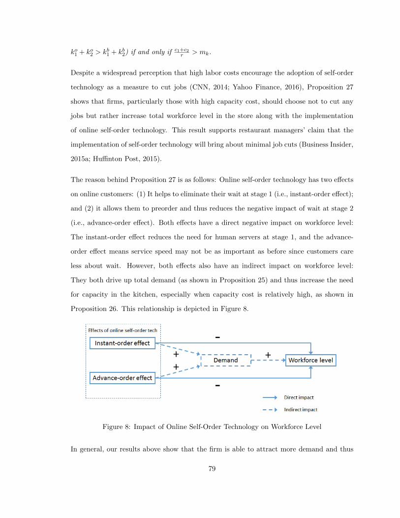
ko1 + ko2 > kb1 + kb2) if and only if c1+c2r > mk.
Despite a widespread perception that high labor costs encourage the adoption of self-order
technology as a measure to cut jobs (CNN, 2014; Yahoo Finance, 2016), Proposition 27
shows that firms, particularly those with high capacity cost, should choose not to cut any
jobs but rather increase total workforce level in the store along with the implementation
of online self-order technology. This result supports restaurant managers’ claim that the
implementation of self-order technology will bring about minimal job cuts (Business Insider,
2015a; Huffinton Post, 2015).
The reason behind Proposition 27 is as follows: Online self-order technology has two effects
on online customers: (1) It helps to eliminate their wait at stage 1 (i.e., instant-order effect);
and (2) it allows them to preorder and thus reduces the negative impact of wait at stage 2
(i.e., advance-order effect). Both effects have a direct negative impact on workforce level:
The instant-order effect reduces the need for human servers at stage 1, and the advance-
order effect means service speed may not be as important as before since customers care
less about wait. However, both effects also have an indirect impact on workforce level:
They both drive up total demand (as shown in Proposition 25) and thus increase the need
for capacity in the kitchen, especially when capacity cost is relatively high, as shown in
Proposition 26. This relationship is depicted in Figure 8.
Figure 8: Impact of Online Self-Order Technology on Workforce Level
In general, our results above show that the firm is able to attract more demand and thus
79
boost sales with online self-order technology. Such increase in total demand is mainly
driven by the fact that online customers are willing to shop more frequently. Meanwhile,
store customers may also choose to increase their shopping rate, as the firm speeds up the
service by increasing the back-end capacity level. Moreover, according to Propositions 25
and 27, if c1+c2r > max(mk,mλ) and θ ∈ (0, ψs), then we find that everyone in the economy
could benefit from the implementation of online self-order technology: both store and online
customers are willing to come to the store more often (i.e., λos > λb, λoo > λb), the firm
obtains more demand (i.e., θλoo + (1− θ)λos > λb), and more workers are hired by the firm
(i.e., ko1 + ko2 > kb1 + kb2).
4.5. Offline Self-Order Technology
In this section, we consider the case where the firm implements the self-order technology
offline, e.g., by providing in-store kiosks and robot waiters. By replacing human servers
with machines, the firm can lower the marginal cost of service interaction at stage 1; this
is the main reason behind many companies’ move to offer offline self-order service (CNN,
2014; Yahoo Finance, 2016). We model this innovation as follows.
There are two types of servers at stage 1: human (with capacity µ1h) and machine (with
capacity µ1m). The cost of human capacity is the same as before, i.e., c1. However, the
cost of machine capacity is c1m. As mentioned above, we assume that it is cheaper to serve
each customer with machine capacity than with human capacity.
In addition, suppose there are two types of customers: A fraction η ∈ (0, 1) of all customers
are tech-savvy and they always prefer to use the self-order machines. On the other hand, the
remaining 1−η are traditional customers who place an order only with human servers; they
may not be comfortable or proficient with using self-order machines. For each type of cus-
tomers, denote their respective wait times at stage 1 as w1m(µ1m,Λ1m) and w1h(µ1h,Λ1h),
where Λ1m and Λ1h are the total demand rates for machine and human capacities at stage
1. Therefore, each type of customer’s shopping rate is given as follows:
80
• tech-savvy customers: λm = [α− β (w1m(µ1m,Λ1m) + w2(µ2,Λ))]+;
• traditional customers: λh = [α− β (w1h(µ1h,Λ1h) + w2(µ2,Λ))]+.
Similar to before, we assume w1m(µ1m,Λ1m) = 1µ1m−Λ1m
and w1h(µ1h,Λ1h) = 1µ1h−Λ1h
.
Given that tech-savvy and traditional customers respectively account for η and 1 − η of
the total population, in equilibrium, we should have Λ1m = ηλm, Λ1h = (1 − η)λh, and
Λ = ηλm + (1− η)λh.
Now, we formulate the firm’s optimization problem. The firm chooses the capacity level at
each stage, i.e., µ1h, µ1m and µ2, to maximize profit rate, as follows.
maxηλm≤µ1m,(1−η)λh≤µ1h,ηλm+(1−η)λh≤µ2
r (ηλm + (1− η)λh)− c1mµ1m − c1µ1h − c2µ2
s.t. λm = [α− β (w1m (µ1m, ηλm) + w2 (µ2, ηλm + (1− η)λh))]+
λh = [α− β (w1h (µ1h, (1− η)λh) + w2 (µ2, ηλm + (1− η)λh))]+
(4.3)
The following proposition gives the optimal solution; we use superscript ·s (for ‘store’) to
denote the case with offline self-order technology.
Proposition 28. ∃α′′ ≥ α′ such that if α > α′′, then there exists a unique optimal solution:
• µs1m = ηλsm +√
βη(r−c1m−c2)c1m
;
• µs1h = (1− η)λsh +√
β(1−η)(r−c1−c2)c1
;
• µs2 = ηλsm + (1− η)λsh +√
β[(r−c1m−c2)η+(r−c1−c2)(1−η)]c2
,
where
• λsm = α− β√
c1mβη(r−c1m−c2) − β
√c2
β[(r−c1m−c2)η+(r−c1−c2)(1−η)] > 0;
• λsh = α− β√
c1β(1−η)(r−c1−c2) − β
√c2
β[(r−c1m−c2)η+(r−c1−c2)(1−η)] > 0.
Otherwise, there does not exist an optimal solution in which both tech-savvy and traditional
81
customers are served.
To focus on the most interesting scenario where the firm serves both tech-savvy and tradi-
tional customers, we assume α > α′′ throughout the study. This assumption implies that
customers value the product sufficiently to generate positive demand at zero wait.
Our model highlights an important consequence of offline self-order technology: it may
create separate waiting lines, one for human servers and one for machines. There are two
reasons for such separation. First, offline technology may exclude a segment of traditional
customers, who have no choice but to wait for human servers. Second, self-ordering in-
novations may be so popular that some customers are willing to wait behind long lines
even when human cashiers are available (Wall Street Journal, 2016b). Consequently, sep-
arate queues may now emerge in place of the single queue in our base model. Although
self-order technology reduces capacity cost and thus encourages capacity investment, the
separate-queues system goes against conventional wisdom of resource pooling and may lead
to higher waiting times. This is particularly so when the capacity costs of humans and
machines are comparable, i.e., c1m ≈ c1. In practice, without dramatic reductions in cost,
it is unlikely that offline self-order technology will be implemented. After all, reducing lines
and saving time at the ordering stage is one of the main reasons why many restaurants
implement self-order machines in the first place (QSR Magazine, 2016).
Lemma 1. There is a threshold c1m ∈ (0, c1) such that average customer wait at stage 1 is
shorter than that in the base model (i.e., ηws1m+ (1−η)ws1h < wb1) if and only if c1m < c1m.
The above result shows that as long as machine capacity cost is below a certain threshold,
the firm can afford to provide ample machine capacity to ensure that the average customer
wait at stage 1 is shorter compared to the base model. Henceforth, we make the following
assumption.
Assumption 1. The capacity cost for machines c1m is sufficiently low. Specifically, c1m <
c1m.
82
In practice, it is widely believed that machines cost significantly less than human employees
(CNN, 2014; Yahoo Finance, 2016). For example, a study by Forrester Research showed
that self-service check-in costs the airlines 16 cents a passenger, compared with $3.68 using
ticket-counter agents (New York Times, 2004). We expect the same magnitude of cost
reduction would apply for self-order machines in a restaurant as well.
The next two propositions characterize customer wait and customer demand in equilibrium,
when offline self-order technology is provided.
Proposition 29. With offline self-order technology,
i. tech-savvy customers wait shorter at stage 1, i.e., ws1m < wb1;
ii. traditional customers wait longer at stage 1, i.e., ws1h > wb1;
iii. everyone waits shorter at stage 2, i.e., ws2 < wb2.
Proposition 30. With offline self-order technology,
i. tech-savvy customers come to the store more often than before, i.e., λsm > λb;
ii. given c1m, c1, c2, traditional customers come to the store more often (i.e., λsh > λb) if
and only if c1+c2r > m′λ and η ∈ (0, ψ′s) for some m′λ ∈ (0, 1) and ψ′s > 0;
iii. total demand increases, i.e., ηλsm + (1− η)λsh > λb.
Propositions 29 and 30 show the changes in customer wait times and shopping rates after
the implementation of offline self-order technology, respectively. Similar to the case with
online self-order technology, we find that the implementation of offline self-order technology
helps to increase total demand. Moreover, the technology is not only beneficial to those
tech-savvy customers who use the machines; it could also benefit traditional customers who
do not adopt the technology.
According to Proposition 30(i), tech-savvy customers shop more frequently than before.
Different from the case with online self-order technology, tech-savvy customers need to
83
share the in-store self-order machines with fellow customers and thus they may still need
to wait to place an order. However, the cheap cost of machines (compared to labor cost)
allows the firm to afford more machine capacity, and thus tech-savvy customers can still
enjoy a shorter wait time with the offline self-order technology compared to the base case.
Proposition 30(ii) implies that the demand from traditional customers may also increase.
This means that traditional customers can also benefit from the implementation of offline
self-order technology, even though they do not use the technology directly. Similar to the
case with online self-order technology, this is mainly because of the potential wait time
reduction at stage 2 rather than at stage 1 (see Proposition 29 (ii) and (iii)). As the next
result confirms, capacity expansion occurs at stage 2 of the service process.
Proposition 31. With offline self-order technology,
i. µs1h < µb1 and µs1m + µs1h > µb1;
ii. µs2 > µb2.
With offline self-order technology, the firm should replace some costly human servers with
cheaper machine servers at stage 1. Therefore, as shown in Proposition 31(i), human capac-
ity in the front end of the store should decrease. But the firm should also increase overall
capacity (i.e., µs1m + µs1h) as the usage of machine capacity brings down average capacity
cost.
Similar to online self-order technology, offline self-order technology could also prompt the
firm to increase the capacity/workforce level at stage 2, as the service cost decreases and
thus the firm can now allocate the extra resources saved from the implementation of cheap
machines at stage 1 to increase the service speed at stage 2 to attract more customers to
the store. However, different from online self-order technology, Proposition 31(ii) implies
that the firm should never decrease the workforce level at stage 2 when the self-order service
is provided offline. The reason is as follows: Online self-order service allows customers to
order ahead of time, and thus online customers can tolerate a longer wait time as they
84
can make better use of the wait time rather than standing in the store; in contrast, with
offline self-order machines, customers still need to come to the store to place the order and
physically wait there for their food to be ready for pickup. Therefore, the firm still needs
to keep a high service rate at stage 2 with offline self-order technology, in order to avoid
customers in the store waiting too long after they place the order.
Although self-order machines should replace some human cashiers at stage 1, Proposi-
tion 31(ii) shows that the firm should also increase capacity in the kitchen area to speed
up the food preparation process. The overall impact on optimal workforce levels is char-
acterized in the next proposition. Note that we employ a similar normalization: given
customer’s average service requirement τ1 and τ2, the corresponding workforce levels at
each stage are ks1 = µs1hτ1 and ks2 = µs2τ2. In particular, at stage 1, human capacity µ1h
generates employment but not machine capacity µ1m.
Proposition 32. Given c1m, c1 and c2, then there exists a threshold m′k ∈ (0, 1) such that
the firm should increase total workforce level after implementing offline self-order technology
(i.e., ks1 + ks2 > kb1 + kb2) if and only if c1+c2r > m′k.
Proposition 32 indicates that the firm may need to increase total workfoce level along with
the implementation of offline self-order technology. This corroborates with McDonald’s
practice in Europe, where they have added more jobs after the implementation of in-store
kiosks (Huffinton Post, 2015). Similar to online self-order technology, Proposition 32 implies
that firms, especially those with high capacity costs (i.e., c1+c2r ), should increase total
workforce level after the implementation of offline self-order technology. The reason is as
follows: In the case of high capacity cost, self-order machines help save a large amount of
labor cost at stage 1. With these savings, the firm can invest more in manpower at stage 2
to further speed up the service and attract more demand to store. Such capacity investment
is more beneficial when the original capacity level is low (due to high capacity cost), because
capacity investments yield economies of scale in a queueing system as mentioned before.
Similar to the online self-order technology, the implementation of offline self-order technol-
85
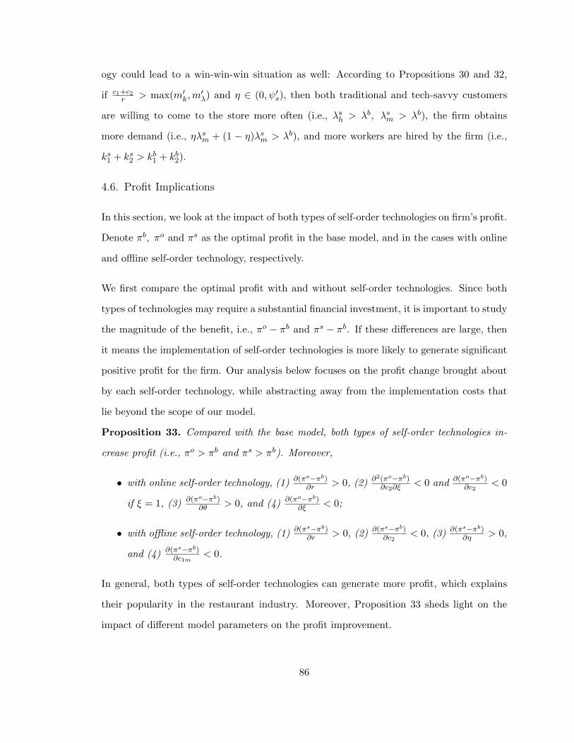
ogy could lead to a win-win-win situation as well: According to Propositions 30 and 32,
if c1+c2r > max(m′k,m
′λ) and η ∈ (0, ψ′s), then both traditional and tech-savvy customers
are willing to come to the store more often (i.e., λsh > λb, λsm > λb), the firm obtains
more demand (i.e., ηλsm + (1 − η)λsm > λb), and more workers are hired by the firm (i.e.,
ks1 + ks2 > kb1 + kb2).
4.6. Profit Implications
In this section, we look at the impact of both types of self-order technologies on firm’s profit.
Denote πb, πo and πs as the optimal profit in the base model, and in the cases with online
and offline self-order technology, respectively.
We first compare the optimal profit with and without self-order technologies. Since both
types of technologies may require a substantial financial investment, it is important to study
the magnitude of the benefit, i.e., πo − πb and πs − πb. If these differences are large, then
it means the implementation of self-order technologies is more likely to generate significant
positive profit for the firm. Our analysis below focuses on the profit change brought about
by each self-order technology, while abstracting away from the implementation costs that
lie beyond the scope of our model.
Proposition 33. Compared with the base model, both types of self-order technologies in-
crease profit (i.e., πo > πb and πs > πb). Moreover,
• with online self-order technology, (1) ∂(πo−πb)∂r > 0, (2) ∂2(πo−πb)
∂c2∂ξ< 0 and ∂(πo−πb)
∂c2< 0
if ξ = 1, (3) ∂(πo−πb)∂θ > 0, and (4) ∂(πo−πb)
∂ξ < 0;
• with offline self-order technology, (1) ∂(πs−πb)∂r > 0, (2) ∂(πs−πb)
∂c2< 0, (3) ∂(πs−πb)
∂η > 0,
and (4) ∂(πs−πb)∂c1m
< 0.
In general, both types of self-order technologies can generate more profit, which explains
their popularity in the restaurant industry. Moreover, Proposition 33 sheds light on the
impact of different model parameters on the profit improvement.
86
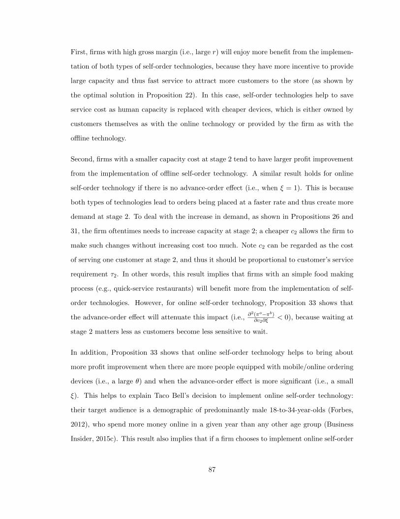
First, firms with high gross margin (i.e., large r) will enjoy more benefit from the implemen-
tation of both types of self-order technologies, because they have more incentive to provide
large capacity and thus fast service to attract more customers to the store (as shown by
the optimal solution in Proposition 22). In this case, self-order technologies help to save
service cost as human capacity is replaced with cheaper devices, which is either owned by
customers themselves as with the online technology or provided by the firm as with the
offline technology.
Second, firms with a smaller capacity cost at stage 2 tend to have larger profit improvement
from the implementation of offline self-order technology. A similar result holds for online
self-order technology if there is no advance-order effect (i.e., when ξ = 1). This is because
both types of technologies lead to orders being placed at a faster rate and thus create more
demand at stage 2. To deal with the increase in demand, as shown in Propositions 26 and
31, the firm oftentimes needs to increase capacity at stage 2; a cheaper c2 allows the firm to
make such changes without increasing cost too much. Note c2 can be regarded as the cost
of serving one customer at stage 2, and thus it should be proportional to customer’s service
requirement τ2. In other words, this result implies that firms with an simple food making
process (e.g., quick-service restaurants) will benefit more from the implementation of self-
order technologies. However, for online self-order technology, Proposition 33 shows that
the advance-order effect will attenuate this impact (i.e., ∂2(πo−πb)∂c2∂ξ
< 0), because waiting at
stage 2 matters less as customers become less sensitive to wait.
In addition, Proposition 33 shows that online self-order technology helps to bring about
more profit improvement when there are more people equipped with mobile/online ordering
devices (i.e., a large θ) and when the advance-order effect is more significant (i.e., a small
ξ). This helps to explain Taco Bell’s decision to implement online self-order technology:
their target audience is a demographic of predominantly male 18-to-34-year-olds (Forbes,
2012), who spend more money online in a given year than any other age group (Business
Insider, 2015c). This result also implies that if a firm chooses to implement online self-order
87
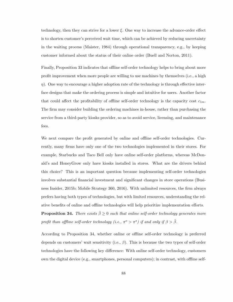
technology, then they can strive for a lower ξ. One way to increase the advance-order effect
is to shorten customer’s perceived wait time, which can be achieved by reducing uncertainty
in the waiting process (Maister, 1984) through operational transparency, e.g., by keeping
customer informed about the status of their online order (Buell and Norton, 2011).
Finally, Proposition 33 indicates that offline self-order technology helps to bring about more
profit improvement when more people are willing to use machines by themselves (i.e., a high
η). One way to encourage a higher adoption rate of the technology is through effective inter-
face designs that make the ordering process is simple and intuitive for users. Another factor
that could affect the profitability of offline self-order technology is the capacity cost c1m.
The firm may consider building the ordering machines in-house, rather than purchasing the
service from a third-party kiosks provider, so as to avoid service, licensing, and maintenance
fees.
We next compare the profit generated by online and offline self-order technologies. Cur-
rently, many firms have only one of the two technologies implemented in their stores. For
example, Starbucks and Taco Bell only have online self-order platforms, whereas McDon-
ald’s and HoneyGrow only have kiosks installed in stores. What are the drivers behind
this choice? This is an important question because implementing self-order technologies
involves substantial financial investment and significant changes in store operations (Busi-
ness Insider, 2015b; Mobile Strategy 360, 2016). With unlimited resources, the firm always
prefers having both types of technologies, but with limited resources, understanding the rel-
ative benefits of online and offline technologies will help prioritize implementation efforts.
Proposition 34. There exists β ≥ 0 such that online self-order technology generates more
profit than offline self-order technology (i.e., πo > πs) if and only if β > β.
According to Proposition 34, whether online or offline self-order technology is preferred
depends on customers’ wait sensitivity (i.e., β). This is because the two types of self-order
technologies have the following key difference: With online self-order technology, customers
own the digital device (e.g., smartphones, personal computers); in contrast, with offline self-
88
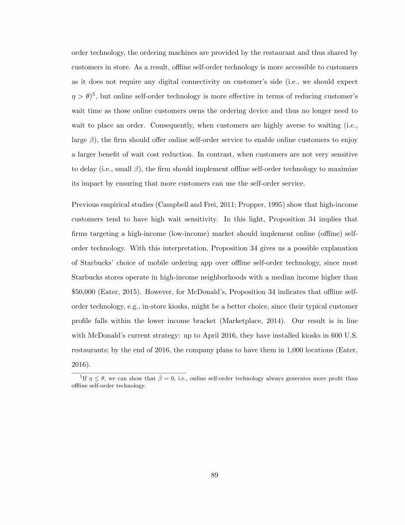
order technology, the ordering machines are provided by the restaurant and thus shared by
customers in store. As a result, offline self-order technology is more accessible to customers
as it does not require any digital connectivity on customer’s side (i.e., we should expect
η > θ)5, but online self-order technology is more effective in terms of reducing customer’s
wait time as those online customers owns the ordering device and thus no longer need to
wait to place an order. Consequently, when customers are highly averse to waiting (i.e.,
large β), the firm should offer online self-order service to enable online customers to enjoy
a larger benefit of wait cost reduction. In contrast, when customers are not very sensitive
to delay (i.e., small β), the firm should implement offline self-order technology to maximize
its impact by ensuring that more customers can use the self-order service.
Previous empirical studies (Campbell and Frei, 2011; Propper, 1995) show that high-income
customers tend to have high wait sensitivity. In this light, Proposition 34 implies that
firms targeting a high-income (low-income) market should implement online (offline) self-
order technology. With this interpretation, Proposition 34 gives us a possible explanation
of Starbucks’ choice of mobile ordering app over offline self-order technology, since most
Starbucks stores operate in high-income neighborhoods with a median income higher than
$50,000 (Eater, 2015). However, for McDonald’s, Proposition 34 indicates that offline self-
order technology, e.g., in-store kiosks, might be a better choice, since their typical customer
profile falls within the lower income bracket (Marketplace, 2014). Our result is in line
with McDonald’s current strategy: up to April 2016, they have installed kiosks in 600 U.S.
restaurants; by the end of 2016, the company plans to have them in 1,000 locations (Eater,
2016).
5If η ≤ θ, we can show that β = 0, i.e., online self-order technology always generates more profit thanoffline self-order technology.
89
4.7. Extensions
4.7.1. Customer Heterogeneity
In our original model, we have assumed that customers have the same base shopping rate
α and wait sensitivity β. We can extend our basic model to incorporate customer hetero-
geneity in these two demand parameters. Suppose tech-savvy customers and traditional
customers have different base shopping rate and wait sensitivity, denoted as αm and αh,
βm and βh, respectively. In the case with online self-order technology, suppose some tech-
savvy customers have access to the online ordering platform and the remaining customers
(e.g., other tech-savvy customers who may not wish to install the app, and all traditional
customers) place an order in the store. In the case with offline self-order technology, all
tech-savvy customers place an order through the machines while all traditional customers
turn to human servers. This extended model can capture customer heterogeneity in terms
of two aspects: (1) Customers may have different loyalty levels towards the firm (which is
reflected by different base shopping rates), and (2) customers may have different sensitivity
levels towards waiting in the store. In Appendix A.6.1, we present a detailed analysis of
this model. Suppose that tech-savvy customers are more wait sensitive than traditional
customers (i.e., βm ≥ βh); this is natural since customers adopt self-order technology pri-
marily because of their impatience with waiting lines (eMarketer, 2014). We find that our
main insights remain valid.
4.7.2. Convex Impact of Wait Time
So far, we have assumed that demand is a linear function of wait time. Our model can be
extended to a more general case where wait time has a convex impact on customer demand
rate. In other words, there is decreasing sensitivity to each additional minute of waiting as
the waiting spells last longer. Specifically, we consider the following demand function:
λ = α− βwφ1 − βwφ2 ,
90
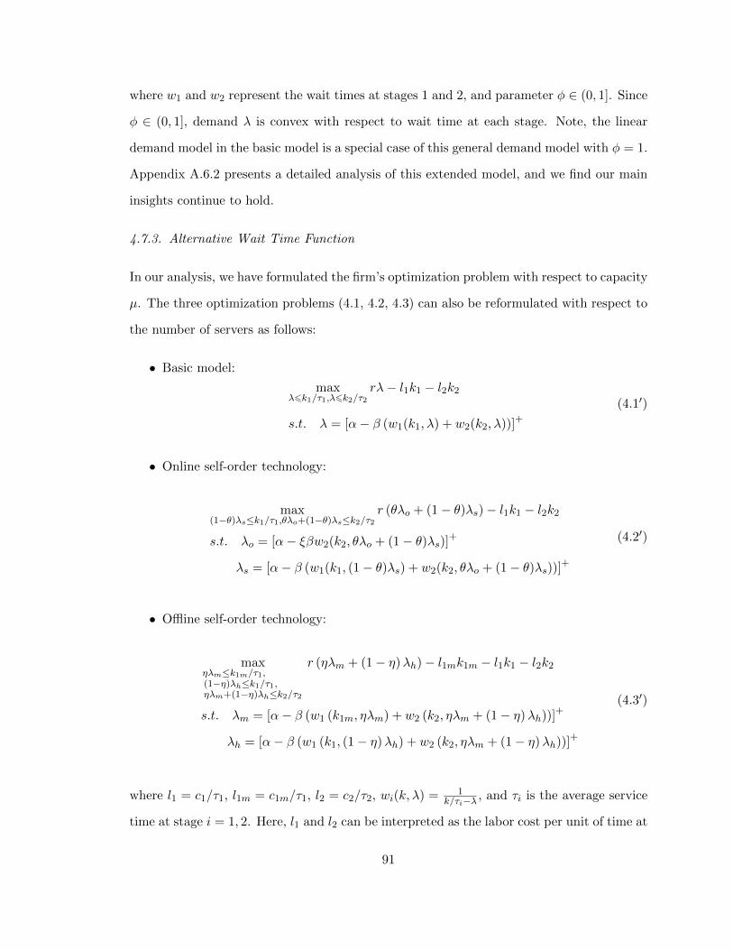
where w1 and w2 represent the wait times at stages 1 and 2, and parameter φ ∈ (0, 1]. Since
φ ∈ (0, 1], demand λ is convex with respect to wait time at each stage. Note, the linear
demand model in the basic model is a special case of this general demand model with φ = 1.
Appendix A.6.2 presents a detailed analysis of this extended model, and we find our main
insights continue to hold.
4.7.3. Alternative Wait Time Function
In our analysis, we have formulated the firm’s optimization problem with respect to capacity
µ. The three optimization problems (4.1, 4.2, 4.3) can also be reformulated with respect to
the number of servers as follows:
• Basic model:
maxλ6k1/τ1,λ6k2/τ2
rλ− l1k1 − l2k2
s.t. λ = [α− β (w1(k1, λ) + w2(k2, λ))]+(4.1′)
• Online self-order technology:
max(1−θ)λs≤k1/τ1,θλo+(1−θ)λs≤k2/τ2
r (θλo + (1− θ)λs)− l1k1 − l2k2
s.t. λo = [α− ξβw2(k2, θλo + (1− θ)λs)]+
λs = [α− β (w1(k1, (1− θ)λs) + w2(k2, θλo + (1− θ)λs))]+
(4.2′)
• Offline self-order technology:
maxηλm≤k1m/τ1,(1−η)λh≤k1/τ1,ηλm+(1−η)λh≤k2/τ2
r (ηλm + (1− η)λh)− l1mk1m − l1k1 − l2k2
s.t. λm = [α− β (w1 (k1m, ηλm) + w2 (k2, ηλm + (1− η)λh))]+
λh = [α− β (w1 (k1, (1− η)λh) + w2 (k2, ηλm + (1− η)λh))]+
(4.3′)
where l1 = c1/τ1, l1m = c1m/τ1, l2 = c2/τ2, wi(k, λ) = 1k/τi−λ , and τi is the average service
time at stage i = 1, 2. Here, l1 and l2 can be interpreted as the labor cost per unit of time at
91
stages 1 and 2, l1m is the corresponding cost for machines. The number of machine servers
is denoted by k1m.
So far, we have assumed wait time function takes the following form: wi(k, λ) = 1k/τi−λ . In
Appendix A.6.3, we numerically test the robustness of our main insights with a different
wait time function, i.e.,
wi(k, λ) =(τik
)ρ√2(k+1)−1
i
1− ρi
+ τi
where ρi = λτik . This corresponds to the approximated average wait time in a M/M/k queue
(Cachon and Terwiesch, 2009). The numerical results show that our main insights remain
valid.
4.8. Conclusion
In 2016, California and New York approved a $15 minimum wage, which doubles the cur-
rent federal minimum. Dramatic increases in labor costs have a significant effect on the
restaurant industry, where profit margins are pennies on the dollar and labor makes up
about a third of total expenses (Wall Street Journal, 2016b). As a result, restaurants are
turning to service automation to reduce cost while maintaining service quality. In this
chapter, we study online and offline self-order technologies, which have been implemented
by an increasing number of restaurants.
We find that self-order technology could benefit everyone in the economy. Customers,
including those who may not have access to the self-order service, would benefit from a
shorter amount of wait time. In addition, the firm is able to provide higher service capacity
level at lower cost. Interestingly, contrary to the public fear that self-service technology
is bound to replace workers, we find that it is sometimes optimal for firms, especially
those with high capacity cost, to increase workforce level after introducing online ordering
platforms or in-store machines. Especially for the quick-service restaurant industry, which
92
is generally a low-margin and high-labor-cost business (Yahoo Finance, 2013), our results
indicate that self-order technologies are more likely to bring about benefits to everyone
including customers, workers, and firms.
Although both online and offline self-order technologies allow customers to place an order
without interacting with a human cashier in the store, each type of technology has different
pros and cons. Online self-order technology offers customers more convenience by allowing
them to preorder using their own digital device, whereas offline self-order technology is more
accessible to customers as the ordering machines are provided in store by the firm. Our
results show that a higher customer wait sensitivity tilts the firm’s optimal choice in favor
of online over offline technologies. Since customers of higher income tend to have higher
wait sensitivity (Campbell and Frei, 2011; Propper, 1995), our results indicate that firms
targeting a high-end market (e.g., Starbucks) should implement online self-order technology
(e.g., mobile ordering app or online ordering website); in contrast, for restaurants whose
customers are mainly in the lower income bracket (e.g., McDonald’s), offline self-order
technology (e.g., in-store kiosks or robot waiters) is more profitable to implement.
Restaurant service includes both ordering and food preparation stages; both require cus-
tomers to wait. Self-order technology helps to shift the workload at the ordering stage from
the firm to customers. Nevertheless, the food preparation stage still requires ample staffing.
This two-stage nature of service processes in the restaurant industry contributes to a shift
of labor from front-end to back-end tasks and possibly to an increase in total workforce
level. However, in some other industries, where self-service technology can cover the entire
service process, it might be inevitable to see workers being replaced by technology. A typi-
cal example is the banking industry, where people can complete most financial transactions
through ATMs and online/mobile channels; this has caused the decline of a large number
of bank branches in the US over the past several years (CNBC, 2015a). We hope our model
in this chapter can contribute to the study of self-service technology in more general ser-
vice processes over a variety of industries. Moreover, some restaurants are even trying to
93
automate the food preparation process using robots (Business Insider, 2016). It would also
be interesting to study the impacts of service automation in the kitchen area, in contrast
to the self-order technology in the front end of the store, on consumer shopping behavior
and restaurant service operations.
94
APPENDIX
A.1. Decentralized System in Heterogeneous Market
Similar to what we did in Section 2.6, we only look at the case where there are some
customers using BOPS, i.e., p−c > wα∗so+α
∗bo
α∗s+α∗b+α∗so+α∗bo−r and α∗b+α∗bo > 0 (see Proposition 7);
otherwise, there would be nobody using BOPS and the issue of revenue allocation becomes
irrelevant as the system collapses into two independent channels.
With revenue sharing parameter θ, the store channel’s profit is given as follows
πs =
(α∗s + α∗so
α∗s + α∗b + α∗so + α∗bo+
α∗b + α∗boα∗s + α∗b + α∗so + α∗bo
θ
)pEmin ((α∗s + α∗b + α∗so + α∗bo)D, q)− cq
+ rEmin ((α∗s + α∗b + α∗so + α∗bo)D, q)
Proposition 35. In the decentralized system, the store will stock q∗ which is given as
follows:
• If(
α∗s+α∗soα∗s+α∗b+α∗so+α
∗bo
+α∗b+α∗bo
α∗s+α∗b+α∗so+α∗boθ)p+ r − c > 0, then
q∗ = (α∗s + α∗b + α∗so + α∗bo) F−1
c(α∗s+α∗so
α∗s+α∗b
+α∗so+α∗bo
+α∗b
+α∗bo
α∗s+α∗b
+α∗so+α∗boθ
)p+r
;
• If(
α∗s+α∗soα∗s+α∗b+α∗so+α
∗bo
+α∗b+α∗bo
α∗s+α∗b+α∗so+α∗boθ)p+ r − c ≤ 0, then q∗ = 0.
Proposition 36. Total profit π∗(θ) is quasiconcave in θ. Moreover,
• Ifα∗b+α∗boα∗so+α
∗bo< w
p , then ∀θ ∈ [0, 1], q∗ > q∗ and π∗(θ) < π∗.
• Ifα∗b+α∗boα∗so+α
∗bo≥ w
p , then
– if θ <(α∗b+α∗bo)p−(α∗so+α
∗bo)w
(α∗b+α∗bo)p, then q∗ < q∗ and π∗(θ) < π∗;
– if θ =(α∗b+α∗bo)p−(α∗so+α
∗bo)w
(α∗b+α∗bo)p, then q∗ = q∗ and π∗(θ) = π∗;
– if θ >(α∗b+α∗bo)p−(α∗so+α
∗bo)w
(α∗b+α∗bo)p, then q∗ > q∗ and π∗(θ) < π∗.
95
Proposition 36 shows that if there are not many people using BOPS (i.e.,α∗b+α∗boα∗so+α
∗bo< w
p or
α∗bp+ α∗bo(p−w) < α∗sow), then there is not enough BOPS revenue for the two channels to
share and thus for the headquarters to fully correct store channels’ incentive: Even if the
store channel is given no credit for fulfilling BOPS demand, i.e., θ = 0, they still stock more
than the system optimal level.
A.2. Model Extensions to Chapter 2
A.2.1. Endogenous Online Channel
In this section, we relax the assumption in the original model that online is exogenous.
Suppose both online and offline follow newsvendor setup. Retail price is p, which is the
same across both channels. Cross-selling benefit in store is r. Unit inventory costs are cs
and co in the store and online channel, both of which are smaller than p. Retailer needs to
decide inventory levels qs and qo in the store and online channel.
Homogeneous Market
Consumers setup is the same as before: They have valuation v for the product and hassle
costs hs, ho, hb. We assume when the online channel is out of stock, those who are willing
to buy online will leave for other websites to buy the product at the same price. Therefore,
given belief about store inventory availability ξ, consumer’s utility from visiting store is the
same as before, i.e., us = −hs + ξ(v − p) + (1 − ξ)(v − p − ho). Consumers compare the
expected utility from each channel and choose accordingly.
Retailer has belief φ about the fraction of customers who visit store. Given this belief, the
retailer’s profit function is
π(qs, qo) = pEmin(φD, qs
)− csqs + rEφD+ pEmin
((1− φ)D +
(φD − qs
)+, qo
)− coqo
(A.1)
Definition 4. A RE equilibrium (qs, qo, φ, φ, ξ) satisfies the following:
96
i Given ξ, if us ≥ uo, then φ = 1; otherwise φ = 0;
ii. Given φ, (qs, qo) = arg maxπ(qs, qo), where π(qs, qo) is given in (A.1);
iii. ξ = A(qs);
iv. φ = φ.
The following proposition gives the RE equilibrium.
Proposition 37. If hs ≤Emin
(D,F−1
(csp
))ED ho and cs < co, then customers visit store and
q◦s = F−1( csp ) and q◦o = 0. Otherwise, no one comes to store and q◦s = 0 and q◦o = F−1( cop ).
With BOPS, retailer’s profit function is as follows:
• If min(hs, hb) > ho, then no one comes to store, and thus
π = pEmin (D, qo)− coqo
• If min(hs, hb) ≤ ho, then consumers come to store if it is in stock, and thus
π = (p+ r)Emin (D, qs)− csqs + pEmin((D − qs)+, qo
)− coqo
Proposition 38. When there is BOPS,
• if min(hs, hb) ≤ ho and cs < co + r, then customers visit store and
– if cs ≤ p+rp co, then q∗s = F−1
(csp+r
)and q∗o = 0;
– if cs >p+rp co, then q∗s = F−1
(cs−cor
)and q∗o = F−1
(cop
)− F−1
(cs−cor
);
• otherwise, no one comes to store and q∗s = 0 and q∗o = F−1(cop
).
Comparing Propositions 37 and 38, we can have the three regions as before, though the
shape is different (see Figure 9).
97
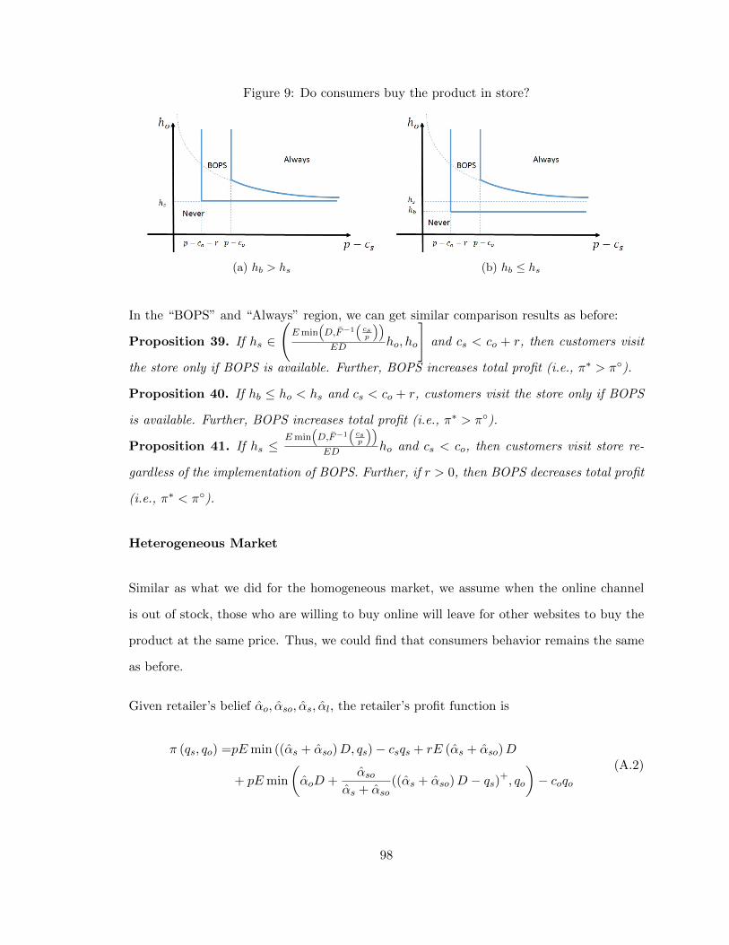
Figure 9: Do consumers buy the product in store?
(a) hb > hs (b) hb ≤ hs
In the “BOPS” and “Always” region, we can get similar comparison results as before:
Proposition 39. If hs ∈
(Emin
(D,F−1
(csp
))ED ho, ho
]and cs < co + r, then customers visit
the store only if BOPS is available. Further, BOPS increases total profit (i.e., π∗ > π◦).
Proposition 40. If hb ≤ ho < hs and cs < co + r, customers visit the store only if BOPS
is available. Further, BOPS increases total profit (i.e., π∗ > π◦).
Proposition 41. If hs ≤Emin
(D,F−1
(csp
))ED ho and cs < co, then customers visit store re-
gardless of the implementation of BOPS. Further, if r > 0, then BOPS decreases total profit
(i.e., π∗ < π◦).
Heterogeneous Market
Similar as what we did for the homogeneous market, we assume when the online channel
is out of stock, those who are willing to buy online will leave for other websites to buy the
product at the same price. Thus, we could find that consumers behavior remains the same
as before.
Given retailer’s belief αo, αso, αs, αl, the retailer’s profit function is
π (qs, qo) =pEmin ((αs + αso)D, qs)− csqs + rE (αs + αso)D
+ pEmin
(αoD +
αsoαs + αso
((αs + αso)D − qs)+, qo
)− coqo
(A.2)
98
Definition 5. A RE equilibrium (αo, αso, , αs, αl, qs, qo, ξ, αo, αso, αs, αl) satisfies the fol-
lowing:
i Given ξ, then αo = v−pH − ξ(v−p)2
2H2 , αso = ξ(v−p)2
2H2 , αs = ξ(v−p)(H−(v−p))H2 , and αl =
[H−(v−p)][H−ξ(v−p)]H2 ;
ii. Given αo, αso, αs and αl, (qs, qo) = arg maxπ(qs, qo), where π(qs, qo) is given in (A.2);
iii. ξ = A(qs), where A(qs) = Emin((αs+αso)D,qs)E(αs+αso)D
;
iv. αs = αs, αo = αo, αso = αso and αl = αl.
Proposition 42.
• If cs <v−p
2H−(v−p)co + 2H−2(v−p)2H−(v−p) p, then there are customers visiting store, specifically,
– if cs < co, then α◦s =ξ◦1(v−p)(H−(v−p))
H2 , α◦so =ξ◦1(v−p)2
2H2 , α◦o = v−pH − ξ◦1(v−p)2
2H2 ,
q◦s = (α◦s + α◦so)F−1( csp ) and q◦o = α◦oF
−1( cop ), where ξ◦1 =min
(D,F−1
(csp
))ED
– if cs ≥ co, then α◦s =ξ◦2(v−p)(H−(v−p))
H2 , α◦so =ξ◦2(v−p)2
2H2 , α◦o = v−pH − ξ◦2(v−p)2
2H2 , q◦s =
(α◦s+α◦so)F
−1
(cs− v−p
2H−(v−p) co2H−2(v−p)2H−(v−p) p
)and q◦o = (α◦o+α
◦so)F
−1( cop )−α◦soF−1
(cs− v−p
2H−(v−p) co2H−2(v−p)2H−(v−p) p
),
where ξ◦2 =
min
D,F−1
cs−v−p
2H−(v−p) co2H−2(v−p)2H−(v−p) p
ED
• If cs ≥ v−p2H−(v−p)co + 2H−2(v−p)
2H−(v−p) p, then no one ever comes to store and q◦s = 0, q◦o =
v−pH F−1( cop ), ξ◦ = 0.
With BOPS, retailer’s profit function is as follows
π (qs, qo) =pEmin ((α∗s + α∗b + α∗so + α∗bo)D, qs)− csqs + rEmin ((α∗s + α∗b + α∗so + α∗bo)D, qs)
+ pEmin
(α∗oD +
α∗so + α∗boα∗s + α∗b + α∗so + α∗bo
((α∗s + α∗b + α∗so + α∗bo)D − qs)+, qo
)− coqo
Proposition 43. Suppose r = 0. When there is BOPS, market outcome is given as follows:
• If cs <α∗so+α
∗bo
α∗s+α∗b+α∗so+α∗boco+
α∗s+α∗bα∗s+α∗b+α∗so+α
∗bop, then there are customers visiting store, and
99
– if cs < co, then q∗s = (α∗s + α∗so)F−1( csp ) and q∗o = α∗oF
−1( cop )
– if cs ≥ co, then q∗s = (α∗s + α∗so)F−1
(cs−
α∗so+α∗boα∗s+α∗
b+α∗so+α∗
boco
α∗s+α∗b
α∗s+α∗b
+α∗so+α∗bop
)and q∗o = (α∗o +
α∗so)F−1( cop )− α∗soF−1
(cs−
α∗so+α∗boα∗s+α∗
b+α∗so+α∗
boco
α∗s+α∗b
α∗s+α∗b
+α∗so+α∗bop
),
• If cs ≥ v−p2H−(v−p)co + 2H−2(v−p)
2H−(v−p) p, then no one ever comes to store and q∗s = 0, q∗o =
v−pH F−1( cop ).
Proposition 44.
i. BOPS helps to expand market coverage, i.e., α∗s +α∗o +α∗b +α∗so+α∗bo > α◦s +α◦o +α◦so;
ii. Suppose r = 0. If there are customers visiting store when there is no BOPS, then there
exists cs such that the implementation of BOPS decreases total profit (i.e., π∗ < π◦)
if βs + βo < 1 and cs > cs.
This shows that although BOPS could expand market coverage, it may still reduce total
profit even if r = 0.
Decentralized System
Finally, let’s look at decentralized system. Here, for simplicity of exposition, we only look at
the homogeneous market. Same as before, we only consider the situation where consumers
use BOPS when it is available. Then, with the revenue sharing parameter θ, store and
online’s profits are given as follows:
πs = (θp+ r)Emin (D, qs)− csqs
πo = (1− θ) pEmin (D, qs) + pEmin((D − qs)+, qo
)− coqo
Note the BOPS revenue is just free money to the online channel. So we only need to
consider store’s incentive. Comparing πs with the centralized profit funtion π, we can
still find that the store channel ignores the fact that customers would buy online instead
100
in case of stockouts (i.e., the second term in πo), and thus there will be a profit loss in
the decentralized system compared to the centralized case. Moreover, it is easy to find
the following revenue sharing parameter will correct store’s incentive and coordinate both
channels:
• If cs ≤ p+rp co, then θ∗ = 1
• If cs >p+rp co, then θ∗ = cor
(cs−co)p ∈ (0, 1).
A.2.2. Default Channel Choice
Suppose a fraction λ of customers are nonstrategic, who head to store by default (because
they may forget or they may not care about checking the website beforehand) and may
consider buying from the online channel only if store is out of stock; the rest 1 − λ are
strategic as before. As a result, when there is BOPS, only a fraction 1−λ of customers will
check online for store inventory information.
Homogeneous Market
Let’s first consider the case when there is no BOPS. Assume all customers (including both
nonstrategic and strategic customers) have the same online hassle cost ho. Then, since
v − p− ho ≥ 0, all nonstrategic customers will buy online if store is out of stock.
The retailer has a belief about the fraction of strategic customers who visit store, denoted
as φ. Given this belief, his total profit is
π =pEmin((λ+ φ(1− λ)
)D, q
)− cq + rE
(λ+ φ(1− λ)
)D
+ wE(1− φ)(1− λ)D + wE((λ+ φ(1− λ)
)D − q
)+
The following proposition gives the RE equilibrium.
Proposition 45. If hs ≤Emin
(D,F−1
(c
p−w
))ED ho and p − c > w, then strategic customers
101
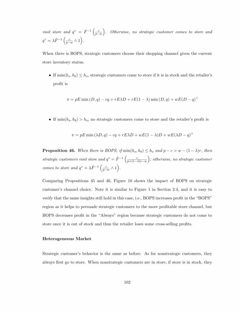
visit store and q◦ = F−1(
cp−w
). Otherwise, no strategic customer comes to store and
q◦ = λF−1(
cp−w ∧ 1
).
When there is BOPS, strategic customers choose their shopping channel given the current
store inventory status.
• If min(hs, hb) ≤ ho, strategic customers come to store if it is in stock and the retailer’s
profit is
π = pEmin (D, q)− cq + rEλD + rE(1− λ) min (D, q) + wE(D − q)+
• If min(hs, hb) > ho, no strategic customers come to store and the retailer’s profit is
π = pEmin (λD, q)− cq + rEλD + wE(1− λ)D + wE(λD − q)+
Proposition 46. When there is BOPS, if min(hs, hb) ≤ ho and p− c > w− (1− λ)r, then
strategic customers visit store and q∗ = F−1(
cp+(1−λ)r−w
); otherwise, no strategic customer
comes to store and q∗ = λF−1(
cp−w ∧ 1
).
Comparing Propositions 45 and 46, Figure 10 shows the impact of BOPS on strategic
customer’s channel choice. Note it is similar to Figure 1 in Section 2.4, and it is easy to
verify that the same insights still hold in this case, i.e., BOPS increases profit in the “BOPS”
region as it helps to persuade strategic customers to the more profitable store channel, but
BOPS decreases profit in the “Always” region because strategic customers do not come to
store once it is out of stock and thus the retailer loses some cross-selling profits.
Heterogeneous Market
Strategic customer’s behavior is the same as before. As for nonstrategic customers, they
always first go to store. When nonstrategic customers are in store, if store is in stock, they
102
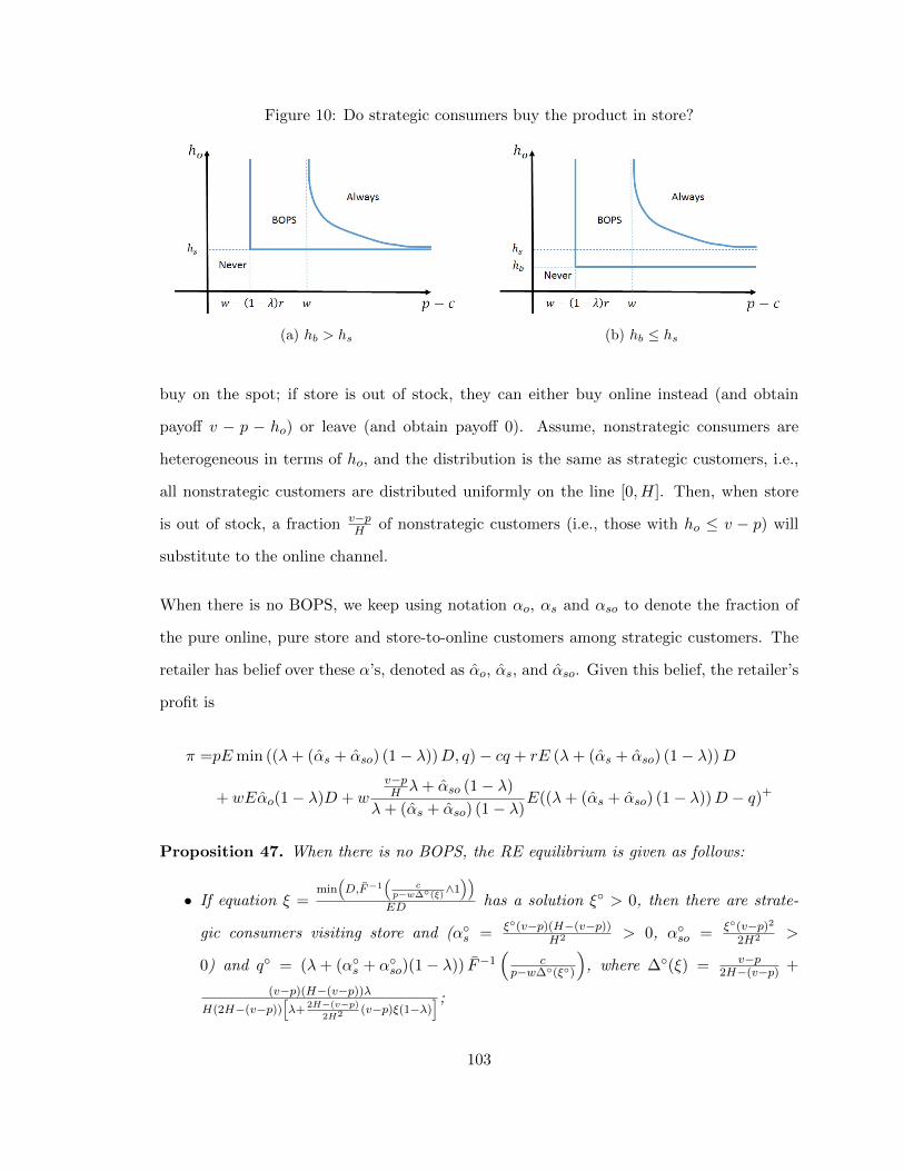
Figure 10: Do strategic consumers buy the product in store?
(a) hb > hs (b) hb ≤ hs
buy on the spot; if store is out of stock, they can either buy online instead (and obtain
payoff v − p − ho) or leave (and obtain payoff 0). Assume, nonstrategic consumers are
heterogeneous in terms of ho, and the distribution is the same as strategic customers, i.e.,
all nonstrategic customers are distributed uniformly on the line [0, H]. Then, when store
is out of stock, a fraction v−pH of nonstrategic customers (i.e., those with ho ≤ v − p) will
substitute to the online channel.
When there is no BOPS, we keep using notation αo, αs and αso to denote the fraction of
the pure online, pure store and store-to-online customers among strategic customers. The
retailer has belief over these α’s, denoted as αo, αs, and αso. Given this belief, the retailer’s
profit is
π =pEmin ((λ+ (αs + αso) (1− λ))D, q)− cq + rE (λ+ (αs + αso) (1− λ))D
+ wEαo(1− λ)D + wv−pH λ+ αso (1− λ)
λ+ (αs + αso) (1− λ)E((λ+ (αs + αso) (1− λ))D − q)+
Proposition 47. When there is no BOPS, the RE equilibrium is given as follows:
• If equation ξ =min
(D,F−1
(c
p−w∆◦(ξ)∧1))
ED has a solution ξ◦ > 0, then there are strate-
gic consumers visiting store and (α◦s = ξ◦(v−p)(H−(v−p))H2 > 0, α◦so = ξ◦(v−p)2
2H2 >
0) and q◦ = (λ+ (α◦s + α◦so)(1− λ)) F−1(
cp−w∆◦(ξ◦)
), where ∆◦(ξ) = v−p
2H−(v−p) +
(v−p)(H−(v−p))λH(2H−(v−p))
[λ+
2H−(v−p)2H2 (v−p)ξ(1−λ)
] ;
103
• otherwise, no strategic customer comes to store and q◦ = 0.
Note a sufficient condition for the equation ξ =min
(D,F−1
(c
p−w∆◦(ξ)∧1))
ED having a positive
solution is p − w∆◦(0) > c. The reason is as follows: If ξ = 1, the left hand side of the
equation is strictly larger than the right hand side; if ξ = 0, when p− w∆◦(0) > c, the left
hand side of the equation is strictly smaller than the right hand side. Since both sides of the
equation are continuous and increasing in ξ, the equation must have a solution ξ◦ ∈ (0, 1).
Next, let’s look at the case when there is BOPS. Note nonstrategic customers will always
first visit store, so they will not be influenced by the information effect. Let’s keep using our
original notations, α∗s, α∗o, α∗b , α∗so, α
∗bo, to denote the fraction of pure store, pure online, pure
BOPS, store-to-online and BOPS-to-online customers among strategic customers. Then,
the retailer’s profit function is
π =pEmin ((λ+ (α∗s + α∗so + α∗b + α∗bo) (1− λ))D, q)− cq + rEλD
+ rE(α∗s + α∗so + α∗b + α∗bo) (1− λ)
λ+(α∗s + α∗so + α∗b + α∗bo
)(1− λ)
min ((λ+ (α∗s + α∗so + α∗b + α∗bo) (1− λ))D, q)
+ wEα∗o(1− λ)D
+ wEv−pH λ+ (α∗so + α∗bo) (1− λ)
λ+(α∗s + α∗so + α∗b + α∗bo
)(1− λ)
((λ+ (α∗s + α∗so + α∗b + α∗bo) (1− λ))D − q)+
Proposition 48. With BOPS, the market outcome is given as follows:
• if p− c > w∆∗ − r (α∗s+α∗so+α∗b+α∗bo)(1−λ)
λ+(α∗s+α∗so+α∗b+α∗bo)(1−λ)
, then there are strategic customers visiting
store and
q∗ = (λ+ (α∗s + α∗so + α∗b + α∗bo) (1− λ)) F−1
c
p− w∆∗ + r(α∗s+α∗so+α
∗b+α∗bo)(1−λ)
λ+(α∗s+α∗so+α∗b+α∗bo)(1−λ)
,
where ∆∗ =v−pH
λ+(α∗so+α∗bo)(1−λ)
λ+(α∗s+α∗so+α∗b+α∗bo)(1−λ)
;
• otherwise, no strategic customer comes to store and q∗ = 0.
104
Proposition 49.
i. BOPS helps to expand market coverage, i.e., λ+ (α∗s + α∗o + α∗b + α∗so + α∗bo)(1− λ) >
λ+ (α◦s + α◦o + α◦so)(1− λ);
ii. Suppose r = 0. If p− w∆◦(0) > c, i.e., there are customers visiting store when there
is no BOPS, then there exist w and βs > 0 such that the implementation of BOPS
decreases total profit (i.e., π∗ < π◦) if βs < βs, w > w and H > v−pβo
.
This shows that although BOPS could expand market coverage, it may still reduce total
profit even if r = 0.
Decentralized System
For simplicity of exposition, let’s only look at the homogeneous market. In a decentralized
system, assuming there are strategic customers using BOPS, the store’s profit is
πs = pEλmin (D, q) + rEλD︸ ︷︷ ︸from nonstrategic customers
+ (θp+ r)E(1− λ) min (D, q)︸ ︷︷ ︸from strategic customers
−cq
Comparing it with the centralized profit function π described above, we find the store’s
incentive is not fully aligned with the system’s. With proper choice of the revenue sharing
parameter θ, we should be able to correct store’s incentive. However, we find that if λ is
very large, we may not have enough BOPS revenue to correct store’s incentive to overstock.
Thus, a simple θ may not be enough to make sure we achieve the centralized profit level.
A.3. Detailed Analyses of Scenarios When Multiple Mechanisms are Provided Simul-
taneously
A.3.1. Providing both Physical Showrooms and Availability Information
With physical showrooms and availability information, consumer utilities are as follows
105
• utility from buying online directly: uo = θ(v − p− ho)− (1− θ)(ho + hr)
• utility from visiting store when store is in stock: us,in = −hs + θ(v − p)
• utility from visiting store when store is out of stock: us,out = −hs + θ(v − p− ho)
Then, if uo < us,out, i.e.,
hs < (1− θ)(ho + hr) (A.3)
consumers would always visit store, even if it is shown that store is out of stock. In this case,
retailer profit is π = pEmin(θD, q)−cq+wE(θD−q)+ = (p−w)Emin(θD, q)−cq+wEθD,
and thus the optimal store inventory level qpa = θF−1(
cp−w
). Note condition (A.3) is
equivalent to θ < ψpa where ψpa = min(max(ho+hr−hsho+hr, 0), 1), given θ ∈ (0, 1).
If uo ∈ [us,out, us,in), i.e.,
hs ∈ [(1− θ)(ho + hr), ho + (1− θ)hr) (A.4)
consumers would visit store if store is in stock but buy online directly if store is out of stock.
In this case, retailer profit π = pEmin(θD, q) − cq + wE(θD − q)+ − rE 1−θθ (θD − q)+ =
(p−w+ r 1−θθ )Emin(θD, q)− cq+ (wθ− r(1− θ))ED, and thus the optimal store inventory
level qpa = θF−1
(c
p−w+r 1−θθ
). Note condition (A.4) is equivalent to θ ∈ [ψpa, ψpa) where
ψpa = min(max(ho+hr−hshr, 0), 1). Moreover, note if the critical fractile c
p−w+r 1−θθ
≥ 1 (⇔
θ ≥ r(w+r−p+c)+ , given θ ∈ (0, 1)), then qpa = 0, i.e., the store never has the product in
stock and thus consumers actually always buy online as a result.
If uo ≥ us,in, i.e., hs ≥ ho+(1−θ)hr or θ ≥ ψpa, then consumers always buy online directly.
In this case, retailer profit π = wEθD − rE(1 − θ)D. The optimal inventory level is just
qpa = 0.
The following proposition summaries the discussion above, where ψpa
= min( r(w+r−p+c)+ , ψ
pa)
Proposition 50. With physical showrooms and availability information, the market out-
106
come is given as follows:
• If θ ≤ ψpa, then consumers always visit store; qpa = θF−1(
cp−w
);
• If θ ∈ [ψpa, ψpa
), then consumers visit the store if it has the product in stock but buy
online directly if store is out of stock; qpa = θF−1
(c
p−w+r 1−θθ
);
• If θ ≥ ψpa, then consumers always buy online directly; qpa = 0.
A.3.2. Providing both Physical Showrooms and Virtual Showrooms
With virtual showrooms, there is a new customer pool. Then, having both physical show-
rooms and virtual showrooms is very similar to the case when there is only physical show-
rooms, simply replacing with a new set of parameters (θ′ and D′ (or F ′)). Thus, similar to
the proof of Proposition 12, we can easily find the RE equilibrium (the proof of which is
omitted):
Proposition 51. With physical showrooms and virtual showrooms, there exists a threshold
ψpv such that
• if θ < ψpv, then consumers visit store; qpv = θ′F ′−1(
cp−w
)• if θ ≥ ψpv, then consumers buy online directly; qpv = 0.
A.3.3. Providing both Virtual Showrooms and Availability Information
Again, note that with virtual showrooms, there is a new customer pool. Then, having both
virtual showrooms and availability information is very similar to the case when there is only
availability information, simply replacing with a new set of parameters (θ′ and D′ (or F ′)).
Thus, similar to the proof of Proposition 16, we can easily find the market outcome (the
proof of which is omitted):
Proposition 52. With virtual showrooms and availability information, there exists a thresh-
old ψva ∈ [ψv, 1] such that the market outcome is given as follows:
107
• If θ < ψva, then consumers visit store if store is in stock, and buy online directly if
store is out of stock; qva = θ′F ′−1(
c
p−w+r 1−θ′θ′
)• If θ ≥ ψva, then consumers always buy online directly; qva = 0.
A.3.4. Providing All Three Mechanisms
Similar to the previous two sections, we note that with virtual showrooms, there is a new
customer pool. Then, having all three mechanisms is very similar to the case when there
are both physical showrooms and availability information, simply replacing with a new set
of parameters (θ′ and D′ (or F ′)). Thus, similar to the discussion in Section A.3.1, we can
easily find the market outcome (the proof of which is omitted):
Proposition 53. With all three types of information, the market outcome is given as fol-
lows:
• If θ < ψpva, then consumers always visit store; qpva = θ′F ′−1(
cp−w
);
• If θ ∈ [ψpva, ψpva
), then consumers visit store if it is in stock but buy online directly
if store is out of stock; qpva = θ′F ′−1(
c
p−w+r 1−θ′θ′
);
• If θ ≥ ψpva, then consumers always buy online directly; qpva = 0.
A.4. Model Extensions to Chapter 3
In Chapter 3, we have the following main findings:
1. Adding physical showrooms may reduce profits.
2. Adding virtual showrooms may reduce profits.
3. Providing only availability information never reduces profits.
4. There is no complementary effect between physical showrooms and availability infor-
mation.
108
5. There is no complementary effect between physical showrooms and virtual showrooms.
In this section, we extend our basic model in three different ways. The goal is to show the
robustness of the results listed above.
A.4.1. Endogenous Online Channel
In this section, we relax the assumption in Chapter 2 that the online channel is exogenous.
Suppose both online and offline channels follow the standard newsvendor setup. The retail
price is p, which is the same across both channels. Unit inventory costs are cs and co in
the store and online channel, both of which are smaller than p. For each unit sold online,
if it is not returned, the retailer can get the revenue p, i.e., the price of the product; if it is
returned, the retailer incurs net cost k (i.e., the retailer cannot make money from dealing
with returns). The retailer decides the inventory levels in both channels, qs and qo, in the
beginning.
Consumers setup is the same as before. We assume when the online channel is out of stock,
those who are willing to buy online will leave for other websites to buy the product at the
same price and obtain the same utility uo. Note, when consumers encounter a stockout
in store, they will buy from the retailer’s online channel first. In many companies (e.g.,
Bonobos and Warby Parker), store employees are trained and equipped with digital devices
to help store customers order online. However, when customers are shopping online at
home, it is hard for a firm to persuade customers to come to store when online is out of
stock. Our model setup is to capture this difference.
With this model setup, we can find that consumer’s utility functions, and thus their channel
choices, remain unchanged.
Base Model
Given belief φ, the retailer’s total profit is
109
• If φ = 1, then
π(qs, qo) = pEmin (θD, qs)− csqs + [pθ − k(1− θ)]Emin
((D − qs
θ
)+, qo
)− coqo
• If φ = 0, then
π(qs, qo) = [pθ − k(1− θ)]Emin (D, qo)− coqo
Definition 6. A RE equilibrium (qs, qo, φ, φ, ξ) satisfies the following:
i Given ξ, if us > uo, then φ = 1; otherwise φ = 0;
ii. Given φ, (qs, qo) = arg maxπ(qs, qo);
iii. ξ = A(qs);
iv. φ = φ.
Proposition 54. In the base model, the RE equilibrium is given as follows:
• If hs < ξ◦1 [ho + (1− θ)hr] and co ≥ [pθ − k(1− θ)] csp , then consumers visit store (i.e.,
φ◦ = 1) and q◦s = θF−1( csp ), q◦o = 0;
• if hs < ξ◦2 [ho + (1 − θ)hr] and co < [pθ − k(1 − θ)] csp and cs ≤ k 1−θθ + co
θ , then
consumers visit store (i.e., φ◦ = 1) and q◦s = θF−1(θcs−cok(1−θ)
), q◦o = F−1
(co
pθ−k(1−θ)
)−
F−1(θcs−cok(1−θ)
);
• otherwise, no one comes to store (i.e., φ◦ = 0) and q◦s = 0, q◦o = F−1(
copθ−k(1−θ)
),
where ξ◦1 =Emin
(D,F−1
(csp
))ED , ξ◦2 =
Emin(D,F−1
(θcs−cok(1−θ)
))ED .
Physical Showrooms
Suppose there is a physical showroom in the store. Given belief φ, the retailer’s total profit
is
110
• If φ = 1, then
π = pEmin (θD, qs)− csqs + pEmin((θD − qs)+, qo
)− coqo
• If φ = 0, then
π = [pθ − k(1− θ)]Emin (D, qo)− coqo
Proposition 55. With physical showrooms, the RE equilibrium is given as follows:
• If hs <Emin
(D,F−1
(csp
))ED θho + (1− θ) (ho + hr) and cs < co, then consumers come to
store (i.e., φp = 1) and qps = θF−1( csp ), qpo = 0;
• if hs < (1− θ)(ho + hr) and cs ≥ co, then consumers come to store (i.e., φp = 1) and
qps = 0, qpo = θF−1( cop );
• otherwise, no one comes to store (i.e., φp = 0) and qps = 0, qpo = F−1(
copθ−k(1−θ)
).
Proposition 56. If (1− θ) (ho + hr) < hs <Emin
(D,F−1
(csp
))ED [ho + (1− θ)hr] and [pθ −
k(1 − θ)] csp < co < cs, then consumers visit store if there is no physical showroom (i.e.,
φ◦ = 1) and they buy online directly if there is physical showroom (i.e., φp = 0). Also, in
this case, physical showroom decreases profit, i.e., π◦ > πp.
This shows that our first finding, i.e., physical showrooms could backfire, is robust.
Virtual Showroom
Suppose there is a virtual showroom online. This is just a special case of the base model,
with D′ and θ′.
Proposition 57. With virtual showrooms, the RE equilibrium is given as follows:
• If hs < ξv1 [ho+ (1−θ′)hr] and co ≥ [pθ′−k(1−θ′)] csp , then consumers visit store (i.e.,
φv = 1) and qvs = θ′F ′−1( csp ), qvo = 0;
111
• if hs < ξv2 [ho + (1− θ′)hr] and co < [pθ′ − k(1− θ′)] csp and cs ≤ k 1−θ′θ′ + co
θ′ , then con-
sumers visit store (i.e., φv = 1) and qvs = θ′F ′−1(θ′cs−cok(1−θ′)
), qvo = F ′−1
(co
pθ′−k(1−θ′)
)−
F ′−1(θ′cs−cok(1−θ′)
);
• otherwise, no one comes to store (i.e., φv = 0) and qvs = 0, qvo = F ′−1(
copθ′−k(1−θ′)
),
where ξv1 =Emin
(D′,F ′−1
(csp
))ED′ , ξv2 =
Emin
(D′,F ′−1
(θ′cs−cok(1−θ′)
))ED′ .
Proposition 58. IfEmin
(D,F−1
(csp
))ED [ho + (1− θ′)hr] < hs <
Emin(D,F−1
(csp
))ED [ho+(1− θ)hr]
and [pθ′− k(1− θ′)] csp < co, then consumers visit store if there is no virtual showroom (i.e.,
φ◦ = 1) and they buy online directly if there is virtual showroom (i.e., φv = 0). Also, in this
case, there exists co such that virtual showroom decreases profit (i.e., π◦ > πv) if co > co.
This shows that our second finding, i.e., virtual showrooms could backfire, is robust.
Availability Information
Suppose there is availability information.
• If hs < ho + (1− θ)hr, then consumers will come to store only if it is in stock. Then,
the retailer’s profit is
π = pEmin (θD, qs)− csqs + [pθ − k(1− θ)]Emin
((D − qs
θ
)+, qo
)− coqo
• If hs ≥ ho + (1− θ)hr, then consumers never come to store. Then, the retailer’s profit
is π = [pθ − k(1− θ)]Emin(D, qo)− coqo.
Proposition 59. With availability information, the market outcome is given as follows:
• If hs < ho + (1 − θ)hr and co ≥ [pθ − k(1− θ)] csp , then consumers visit store if store
is in stock and qas = θF−1( csp ), qao = 0;
• if hs < ho + (1 − θ)hr and co < [pθ − k(1 − θ)] csp and cs ≤ k 1−θθ + co
θ , then con-
112
sumers visit store if store is in stock and qas = θF−1(θcs−cok(1−θ)
), qao = F−1
(co
pθ−k(1−θ)
)−
F−1(θcs−cok(1−θ)
);
• otherwise, no one ever comes to store and qas = 0, qao = F−1(
copθ−k(1−θ)
),
Proposition 60. Availability info never reduces profit, i.e., πa ≥ π◦.
This shows that our third finding, i.e., availability information never reduces profit, is
robust.
Joint Implementation
Here, we only look at the two pairs, i.e., physical showrooms and availability information,
and physical showrooms and virtual showrooms. Our goal is to check if there is any com-
plementary effect between them.
Suppose there are both physical showrooms and availability information.
• If hs < (1− θ)(ho + hr), then consumers would always visit store. Thus,
π = pEmin (θD, qs)− csqs + pEmin((θD − qs)+, qo
)− coqo
• if (1 − θ)(ho + hr) ≤ hs < ho + (1 − θ)hr, then consumers come to store only if it is
in stock. Thus,
π = pEmin (θD, qs)− csqs + [pθ − k (1− θ)]Emin
((D − qs
θ
)+, qo
)− coqo
• if hs ≥ ho + (1− θ)hr, then no one ever comes to store. Thus,
π = [pθ − k (1− θ)]Emin (D, qo)− coqo
Proposition 61. πpa ≤ max(πp, πa)
113
This shows that there is no complementary effect between physical showroom and availabil-
ity information.
Suppose there are both physical and virtual showrooms. This is just the same as the physical
showroom only scenario with a different customer pool D′ and θ′.
Proposition 62. πpv ≤ max(πp, πv)
This shows that there is no complementary effect between these two types of showrooms.
A.4.2. Continuous Valuation
Suppose consumer valuation V is continuously distributed on [0,+∞). Let G(v) be the
proportion of consumers with a valuation v or lower. Ex ante, consumers know the distri-
bution G but not their valuations, so they are homogeneous. Ex post, consumers will learn
their valuations after purchase or by checking the product in store.
All other model elements remain the same as before.
Base Model
If consumers buy online directly, after they get the delivery, they can realize their valuation.
For a consumer with V , if she keeps it, she gets payoff V − p − ho; if she returns it, her
payoff is −ho − hr. Then, only those with V < p− hr will return the product. The ex ante
expected payoff of buying online directly is
uo = EV max(V − p− ho,−ho − hr)
Note those with V ∈ (p−hr, p) will not like the product (since V < p) but they don’t return
it because the return cost is too high (since V − p > −hr).
In the store, if there is stock, then consumers can realize their valuation, and only those
with V ≥ p will make a purchase on the spot, and the others will leave. If store is out of
114
stock, they can buy online. So the expected payoff is
us(ξ) = −hs + ξEV max(V − p, 0) + (1− ξ)uo
Here, as what we did in Chapter 2, we assume consumers would consider both channels,
i.e., uo ≥ 0 and us(1) ≥ 0.
Denote the fraction of customers who visit store as φ. In an equilibrium, this could be
either 0 or 1, since consumers are ex ante homogeneous.
Given belief φ, the retailer’s profit function is
π(q) =pG (p)EDDin (q)− cq (A.5)
+[wG (p− hr)− rG (p− hr)
]EDDout (q) (A.6)
+[wG (p− hr)− rG (p− hr)
] (1− φ
)EDD (A.7)
where Din(q) = min(φD, qG(p)
), and Dout(q) = (φD − qG(p)
)+.
Definition 7. A RE equilibrium (q, φ, φ, ξ) satisfies the following:
i Given ξ, if us > uo, then φ = 1; otherwise φ = 0;
ii. Given φ, q = arg maxπ(q);
iii. ξ = A(q), where A(q) = min(φD,q/G(p))EφD ;
iv. φ = φ.
Proposition 63. If hs < h◦s, then consumers visit store (i.e., φ◦ = 1) and
q◦ = G (p) F−1
(c
p−w G(p−hr)
G(p)+r
G(p−hr)
G(p)
), where h◦s = ξ◦(EV max(V −p, 0)+ho−EV max(V −
p,−hr)) and ξ◦ =
ED min
D,F−1
c
p−w G(p−hr)G(p)
+rG(p−hr)G(p)
EDD
; otherwise, no one comes to store
(i.e., φ◦ = 0), and q◦ = 0.
115
Physical Showrooms
With physical showrooms, when store is out of stock, consumers are still able to realize
their valuation. In such case, only those store customers with V − p− ho ≥ 0 will keep on
buying online. So
us(ξ) = −hs + ξEV max(V − p, 0) + (1− ξ)EV max(V − p− ho, 0)
Then, the retailer’s profit is
π =pG (p)EDDin (q)− cq (A.8)
+ wG(p+ ho)EDDout (q) (A.9)
+[wG (p− hr)− rG (p− hr)
] (1− φ
)EDD (A.10)
where Din(q) = min(φD, qG(p)
), and Dout(q) = (φD − qG(p)
)+.
Proposition 64. With physical showrooms, if hs < hps, then consumers visit store (i.e.,
φp = 1), and qp = G (p) F−1
(c
p−w G(p+ho)
G(p)
), where hps = ξpEv max(V − p, 0) + (1 −
ξp)EV max(V −p−ho, 0)+ho−EV max(V −p,−hr) and ξp =
ED min
D,F−1
c
p−w G(p+ho)G(p)
EDD
;
otherwise, no one comes to store (i.e., φp = 0), and qp = 0. Moreover, hps > h◦s if and only
if r is small enough.
Proposition 65. If hps < h◦s and hs ∈ [hps, h◦s), then consumers come to store in the base
case but buy online directly if there is physical showroom. As a result, providing physical
showrooms reduces total profit (i.e., πp < π◦).
This shows that our first finding, i.e., physical showrooms could backfire, is robust.
116
Virtual Showrooms
Similar to what we did in Chapter 3, we assume virtual showrooms help to screen out some
“low-type” customers. Specifically, the signal consumers receive after checking with the
virtual showroom is still binary: those whose valuation V < v will realize their valuation
is low and therefore leave the market without any purchase, while those whose valuation
V ≥ v will know their valuation is greater than v and update their belief about the valuation
distribution to G′ such that ∀v ≥ v, G′(v) = G(v)−G(v)1−G(v) . Here, we assume threshold v ≤
p−hr, i.e., virtual showrooms would screen out only those who really don’t like the product
and are bound to return the product if they buy it online. The total number of customers
left in the market is D′ = [1−G(v)]D.
Thus, the model is the same as base model except for a new customer pool, D′ and G′. We
denote E′V as the expectation over V given G′.
Proposition 66. With virtual showrooms, if hs < hvs, then consumers visit store (i.e.,
φv = 1), and qv = G (p) F−1
(c
p−w G′(p−hr)
G′(p) +rG′(p−hr)
G′(p)
), where hvs = ξv(E′V max(V − p, 0) +
ho − E′V max(V − p,−hr)) and ξv =
ED min
D,F−1
c
p−w G′(p−hr)G′(p) +r
G′(p−hr)G′(p)
EDD
; otherwise, no
one comes to store (i.e., φv = 0), and qv = 0. Moreover, hvs < h◦s.
Proposition 67. If hs ∈ [hvs , h◦s), then consumers come to store in the base case but buy
online directly if there is virtual showroom. As a result, there exists w such that providing
virtual showrooms reduces total profit (i.e., πv < π◦) if w < w.
This shows that our second finding, i.e., virtual showrooms could backfire, is robust.
Availability Information
With availability information, if it is shown that store is in stock, then us,in = −hs +
EV max(V − p, 0). Apparently, consumer will not go to store if store is out of stock.
117
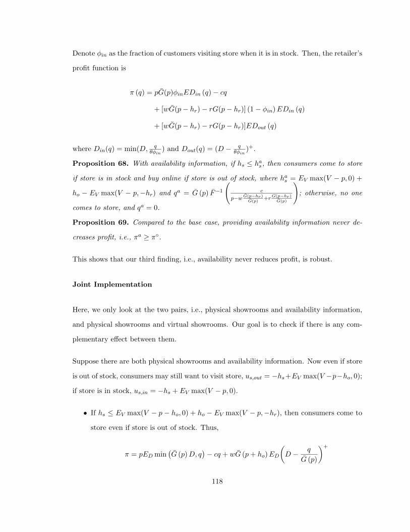
Denote φin as the fraction of customers visiting store when it is in stock. Then, the retailer’s
profit function is
π (q) = pG(p)φinEDin (q)− cq
+ [wG(p− hr)− rG(p− hr)] (1− φin)EDin (q)
+ [wG(p− hr)− rG(p− hr)]EDout (q)
where Din(q) = min(D, qθφin
) and Dout(q) = (D − qθφin
)+.
Proposition 68. With availability information, if hs ≤ has , then consumers come to store
if store is in stock and buy online if store is out of stock, where has = EV max(V − p, 0) +
ho − EV max(V − p,−hr) and qa = G (p) F−1
(c
p−w G(p−hr)
G(p)+r
G(p−hr)
G(p)
); otherwise, no one
comes to store, and qa = 0.
Proposition 69. Compared to the base case, providing availability information never de-
creases profit, i.e., πa ≥ π◦.
This shows that our third finding, i.e., availability never reduces profit, is robust.
Joint Implementation
Here, we only look at the two pairs, i.e., physical showrooms and availability information,
and physical showrooms and virtual showrooms. Our goal is to check if there is any com-
plementary effect between them.
Suppose there are both physical showrooms and availability information. Now even if store
is out of stock, consumers may still want to visit store, us,out = −hs+EV max(V −p−ho, 0);
if store is in stock, us,in = −hs + EV max(V − p, 0).
• If hs ≤ EV max(V − p − ho, 0) + ho − EV max(V − p,−hr), then consumers come to
store even if store is out of stock. Thus,
π = pED min(G (p)D, q
)− cq + wG (p+ ho)ED
(D − q
G (p)
)+
118
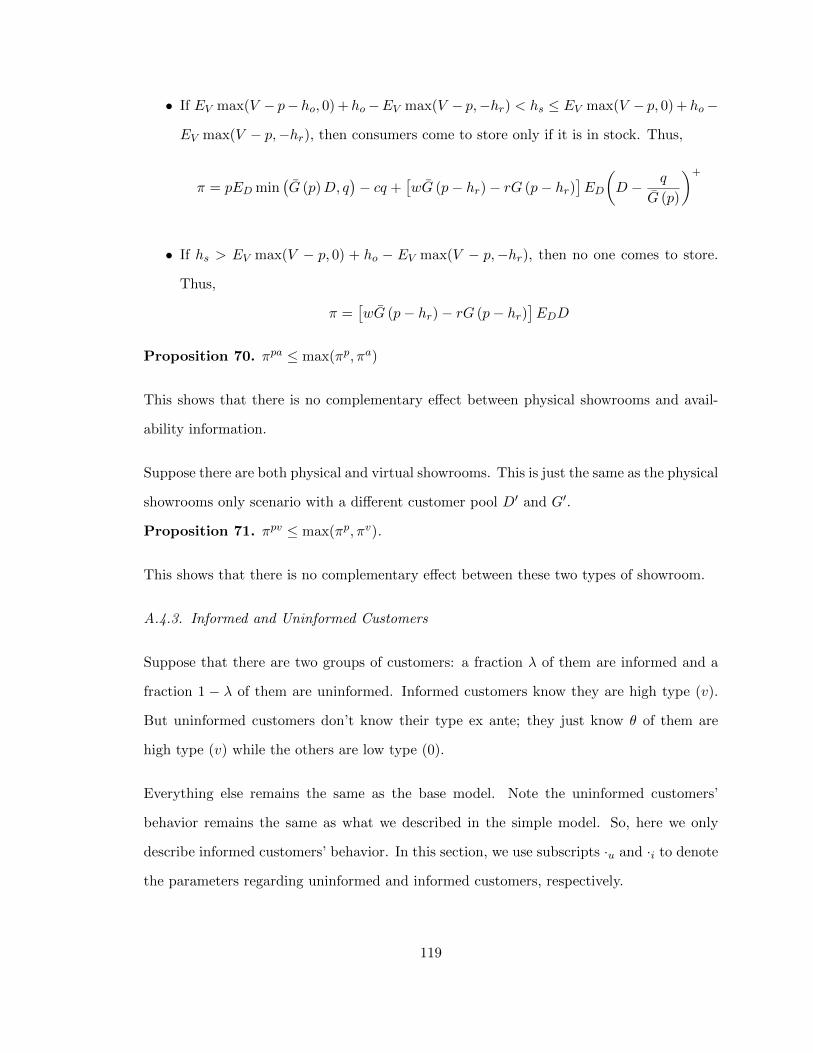
• If EV max(V − p−ho, 0) +ho−EV max(V − p,−hr) < hs ≤ EV max(V − p, 0) +ho−
EV max(V − p,−hr), then consumers come to store only if it is in stock. Thus,
π = pED min(G (p)D, q
)− cq +
[wG (p− hr)− rG (p− hr)
]ED
(D − q
G (p)
)+
• If hs > EV max(V − p, 0) + ho − EV max(V − p,−hr), then no one comes to store.
Thus,
π =[wG (p− hr)− rG (p− hr)
]EDD
Proposition 70. πpa ≤ max(πp, πa)
This shows that there is no complementary effect between physical showrooms and avail-
ability information.
Suppose there are both physical and virtual showrooms. This is just the same as the physical
showrooms only scenario with a different customer pool D′ and G′.
Proposition 71. πpv ≤ max(πp, πv).
This shows that there is no complementary effect between these two types of showroom.
A.4.3. Informed and Uninformed Customers
Suppose that there are two groups of customers: a fraction λ of them are informed and a
fraction 1 − λ of them are uninformed. Informed customers know they are high type (v).
But uninformed customers don’t know their type ex ante; they just know θ of them are
high type (v) while the others are low type (0).
Everything else remains the same as the base model. Note the uninformed customers’
behavior remains the same as what we described in the simple model. So, here we only
describe informed customers’ behavior. In this section, we use subscripts ·u and ·i to denote
the parameters regarding uninformed and informed customers, respectively.
119
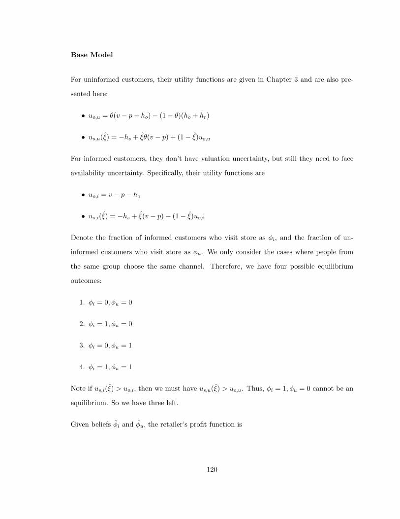
Base Model
For uninformed customers, their utility functions are given in Chapter 3 and are also pre-
sented here:
• uo,u = θ(v − p− ho)− (1− θ)(ho + hr)
• us,u(ξ) = −hs + ξθ(v − p) + (1− ξ)uo,u
For informed customers, they don’t have valuation uncertainty, but still they need to face
availability uncertainty. Specifically, their utility functions are
• uo,i = v − p− ho
• us,i(ξ) = −hs + ξ(v − p) + (1− ξ)uo,i
Denote the fraction of informed customers who visit store as φi, and the fraction of un-
informed customers who visit store as φu. We only consider the cases where people from
the same group choose the same channel. Therefore, we have four possible equilibrium
outcomes:
1. φi = 0, φu = 0
2. φi = 1, φu = 0
3. φi = 0, φu = 1
4. φi = 1, φu = 1
Note if us,i(ξ) > uo,i, then we must have us,u(ξ) > uo,u. Thus, φi = 1, φu = 0 cannot be an
equilibrium. So we have three left.
Given beliefs φi and φu, the retailer’s profit function is
120
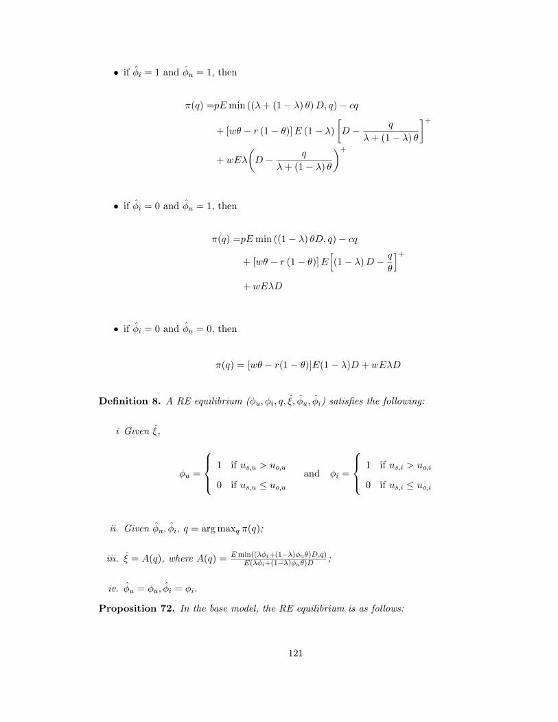
• if φi = 1 and φu = 1, then
π(q) =pEmin ((λ+ (1− λ) θ)D, q)− cq
+ [wθ − r (1− θ)]E (1− λ)
[D − q
λ+ (1− λ) θ
]+
+ wEλ
(D − q
λ+ (1− λ) θ
)+
• if φi = 0 and φu = 1, then
π(q) =pEmin ((1− λ) θD, q)− cq
+ [wθ − r (1− θ)]E[(1− λ)D − q
θ
]+
+ wEλD
• if φi = 0 and φu = 0, then
π(q) = [wθ − r(1− θ)]E(1− λ)D + wEλD
Definition 8. A RE equilibrium (φu, φi, q, ξ, φu, φi) satisfies the following:
i Given ξ,
φu =
1 if us,u > uo,u
0 if us,u ≤ uo,uand φi =
1 if us,i > uo,i
0 if us,i ≤ uo,i
ii. Given φu, φi, q = arg maxq π(q);
iii. ξ = A(q), where A(q) = Emin((λφi+(1−λ)φuθ)D,q)E(λφi+(1−λ)φuθ)D
;
iv. φu = φu, φi = φi.
Proposition 72. In the base model, the RE equilibrium is as follows:
121
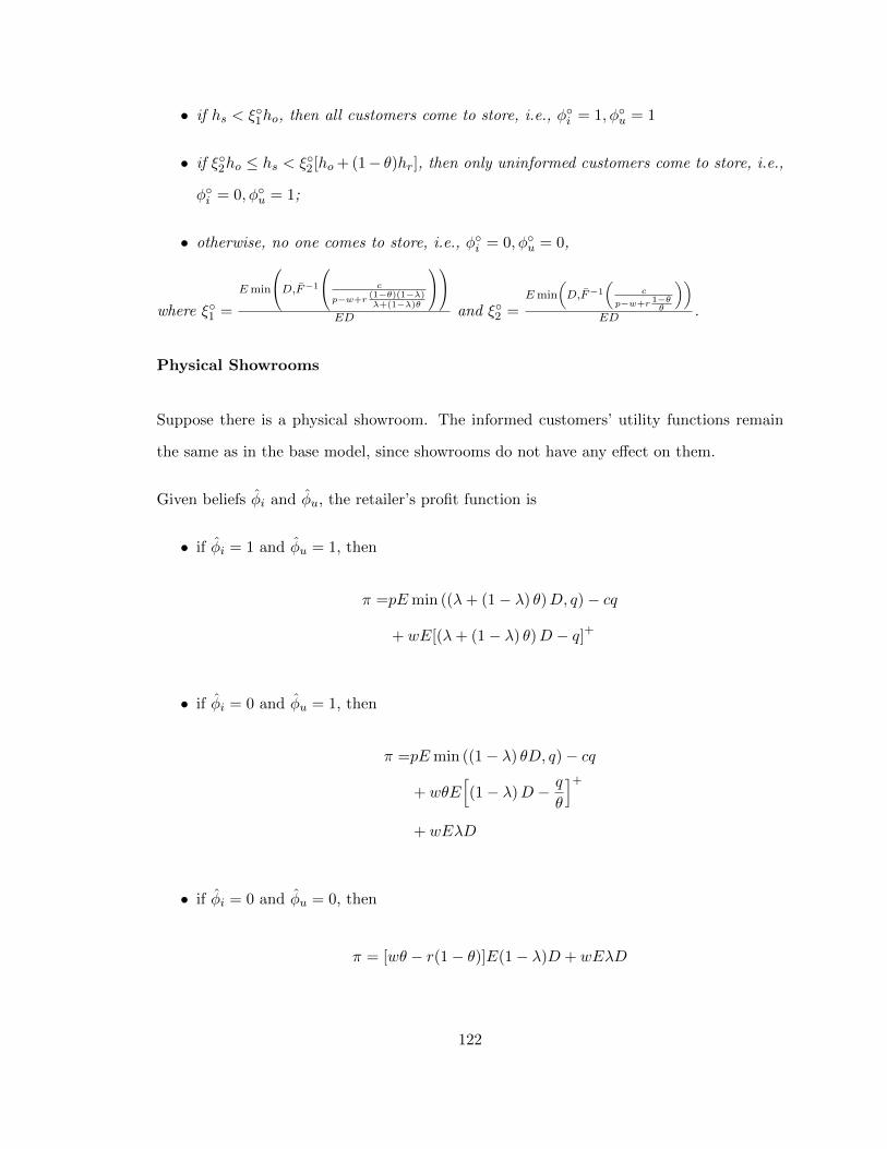
• if hs < ξ◦1ho, then all customers come to store, i.e., φ◦i = 1, φ◦u = 1
• if ξ◦2ho ≤ hs < ξ◦2 [ho + (1− θ)hr], then only uninformed customers come to store, i.e.,
φ◦i = 0, φ◦u = 1;
• otherwise, no one comes to store, i.e., φ◦i = 0, φ◦u = 0,
where ξ◦1 =
Emin
D,F−1
c
p−w+r(1−θ)(1−λ)λ+(1−λ)θ
ED and ξ◦2 =
Emin
(D,F−1
(c
p−w+r 1−θθ
))ED .
Physical Showrooms
Suppose there is a physical showroom. The informed customers’ utility functions remain
the same as in the base model, since showrooms do not have any effect on them.
Given beliefs φi and φu, the retailer’s profit function is
• if φi = 1 and φu = 1, then
π =pEmin ((λ+ (1− λ) θ)D, q)− cq
+ wE[(λ+ (1− λ) θ)D − q]+
• if φi = 0 and φu = 1, then
π =pEmin ((1− λ) θD, q)− cq
+ wθE[(1− λ)D − q
θ
]+
+ wEλD
• if φi = 0 and φu = 0, then
π = [wθ − r(1− θ)]E(1− λ)D + wEλD
122
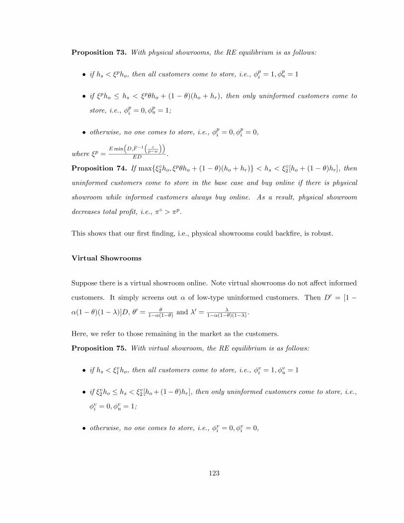
Proposition 73. With physical showrooms, the RE equilibrium is as follows:
• if hs < ξpho, then all customers come to store, i.e., φpi = 1, φpu = 1
• if ξpho ≤ hs < ξpθho + (1 − θ)(ho + hr), then only uninformed customers come to
store, i.e., φpi = 0, φpu = 1;
• otherwise, no one comes to store, i.e., φpi = 0, φpi = 0,
where ξp =Emin
(D,F−1
(c
p−w
))ED .
Proposition 74. If max{ξ◦2ho, ξpθho + (1 − θ)(ho + hr)} < hs < ξ◦2 [ho + (1 − θ)hr], then
uninformed customers come to store in the base case and buy online if there is physical
showroom while informed customers always buy online. As a result, physical showroom
decreases total profit, i.e., π◦ > πp.
This shows that our first finding, i.e., physical showrooms could backfire, is robust.
Virtual Showrooms
Suppose there is a virtual showroom online. Note virtual showrooms do not affect informed
customers. It simply screens out α of low-type uninformed customers. Then D′ = [1 −
α(1− θ)(1− λ)]D, θ′ = θ1−α(1−θ) and λ′ = λ
1−α(1−θ)(1−λ) .
Here, we refer to those remaining in the market as the customers.
Proposition 75. With virtual showroom, the RE equilibrium is as follows:
• if hs < ξv1ho, then all customers come to store, i.e., φvi = 1, φvu = 1
• if ξv2ho ≤ hs < ξv2 [ho + (1− θ)hr], then only uninformed customers come to store, i.e.,
φvi = 0, φvu = 1;
• otherwise, no one comes to store, i.e., φvi = 0, φvi = 0,
123
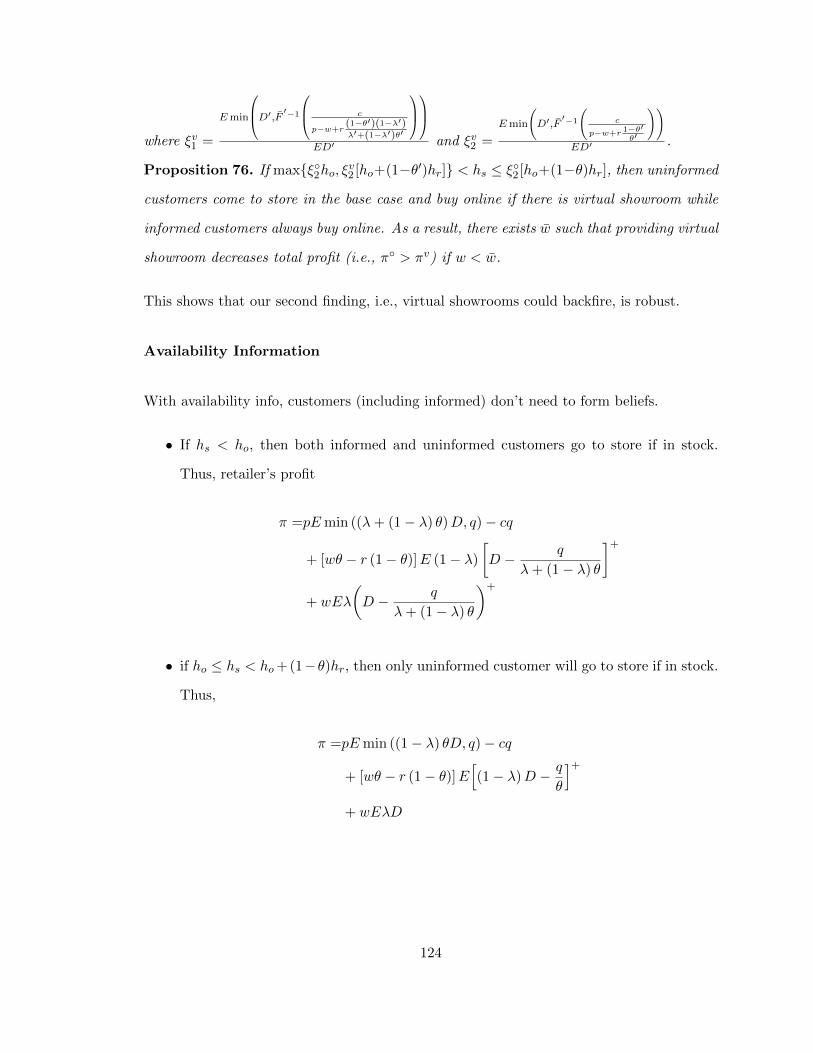
where ξv1 =
Emin
D′,F ′−1
c
p−w+r(1−θ′)(1−λ′)λ′+(1−λ′)θ′
ED′ and ξv2 =
Emin
(D′,F
′−1
(c
p−w+r 1−θ′θ′
))ED′ .
Proposition 76. If max{ξ◦2ho, ξv2 [ho+(1−θ′)hr]} < hs ≤ ξ◦2 [ho+(1−θ)hr], then uninformed
customers come to store in the base case and buy online if there is virtual showroom while
informed customers always buy online. As a result, there exists w such that providing virtual
showroom decreases total profit (i.e., π◦ > πv) if w < w.
This shows that our second finding, i.e., virtual showrooms could backfire, is robust.
Availability Information
With availability info, customers (including informed) don’t need to form beliefs.
• If hs < ho, then both informed and uninformed customers go to store if in stock.
Thus, retailer’s profit
π =pEmin ((λ+ (1− λ) θ)D, q)− cq
+ [wθ − r (1− θ)]E (1− λ)
[D − q
λ+ (1− λ) θ
]+
+ wEλ
(D − q
λ+ (1− λ) θ
)+
• if ho ≤ hs < ho+(1−θ)hr, then only uninformed customer will go to store if in stock.
Thus,
π =pEmin ((1− λ) θD, q)− cq
+ [wθ − r (1− θ)]E[(1− λ)D − q
θ
]+
+ wEλD
124
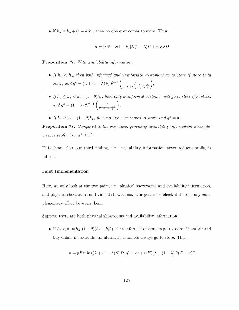
• if hs ≥ ho + (1− θ)hr, then no one ever comes to store. Thus,
π = [wθ − r(1− θ)]E(1− λ)D + wEλD
Proposition 77. With availability information,
• If hs < ho, then both informed and uninformed customers go to store if store is in
stock, and qa = (λ+ (1− λ) θ) F−1
(c
p−w+r(1−λ)(1−θ)λ+(1−λ)θ
);
• If ho ≤ hs < ho+(1−θ)hr, then only uninformed customer will go to store if in stock,
and qa = (1− λ) θF−1
(c
p−w+r 1−θθ
);
• If hs ≥ ho + (1− θ)hr, then no one ever comes to store, and qa = 0.
Proposition 78. Compared to the base case, providing availability information never de-
creases profit, i.e., πa ≥ π◦.
This shows that our third finding, i.e., availability information never reduces profit, is
robust.
Joint Implementation
Here, we only look at the two pairs, i.e., physical showrooms and availability information,
and physical showrooms and virtual showrooms. Our goal is to check if there is any com-
plementary effect between them.
Suppose there are both physical showrooms and availability information.
• If hs < min(ho, (1− θ)(ho + hr)), then informed customers go to store if in-stock and
buy online if stockouts; uninformed customers always go to store. Thus,
π = pEmin ((λ+ (1− λ) θ)D, q)− cq + wE((λ+ (1− λ) θ)D − q)+
125
• If ho < (1 − θ)(ho + hr) and ho ≤ hs < (1 − θ)(ho + hr), then informed customers
always buy online; uninformed customers always go to store. Thus,
π = pEmin ((1− λ) θD, q)− cq + wE((1− λ) θD − q)+ + wEλD
• If ho > (1− θ)(ho + hr) and (1− θ)(ho + hr) ≤ hs < ho, then informed customers go
to store if in stock and buy online if stockouts; uninformed customers go to stock if
in stock and buy online if stockouts. Thus,
π =pEmin ((λ+ (1− λ) θ)D, q)− cq
+ [wθ − r (1− θ)]E (1− λ)
[D − q
λ+ (1− λ) θ
]+
+ wEλ
(D − q
λ+ (1− λ) θ
)+
• If max(ho, (1 − θ)(ho + hr)) ≤ hs < ho + (1 − θ)hr, then informed customers always
buy online; uninformed customers go to store if in stock and buy online if out of stock.
Thus,
π =pEmin ((1− λ) θD, q)− cq
+ [wθ − r (1− θ)]E[(1− λ)D − q
θ
]+
+ wEλD
• If hs ≥ ho + (1− θ)hr, then no one ever comes to store. Thus,
π = [wθ − r(1− θ)]E(1− λ)D + wEλD
Proposition 79. πpa > max(πp, πa) if and only if ξpho < hs < min(ho, (1− θ)(ho + hr)).
Let us compare consumer equilibrium behavior in the three scenarios when ξpho < hs <
126
min(ho, (1− θ)(ho + hr):
i. Physical showrooms only:
– informed customer: buy online
– uninformed customer: go to store
ii. Availability information only:
– informed customer: go to store if in stock, buy online if stockouts
– uninformed customer: go to store if in stock, buy online if stockouts
iii. Physical showrooms and availability information:
– informed customer: go to store if in stock, buy online if stockouts
– uninformed customer: always go to store
Proposition 79 shows that when different types of customers require different types of in-
formation, we may need to offer both physical showroom and availability info. Specifically,
we need physical showrooms to attract uninformed customer, and availability information
to attract informed customers to the store.
Suppose there are both physical and virtual showrooms. This is similar to the physical
showrooms only scenario with D′, θ′ and λ′.
Proposition 80. πpv ≤ max(πp, πv).
This shows that there is no complementary effect between these two types of showrooms.
A.5. Numerical Study for Chapter 3
The goals of this numerical study are as follows:
1. Investigate the likelihood of π◦ > πp;
127
2. Investigate the likelihood of π◦ > πv.
Here, we consider the following parameter values:
• v = 60
• p = 30, w = 15
• p−cw = {0.6, 0.7, 0.8, 0.9, 1, 1.1, 1.2, 1.3, 1.4}
• r = {1, 3, 5, 7, 9}
• ho = {1, 2, 3, 4, 5}
• hs = {1, 2, 3, 4, 5}
• hr = {1, 2, 3, 4, 5}
• D ∼ N(µ, σ2), where µ = 100, σµ = {1
4 ,1
4.5 ,15 ,
15.5 ,
16 ,
16.5 ,
17 ,
17.5 ,
18}
• α = {0.1, 0.3, 0.5, 0.7, 0.9}
• θ = {0.1, 0.3, 0.5, 0.7, 0.9}
There are 1,265,625 cases in total. After checking with the assumptions we made in Chap-
ter 3, we end up having 914,895 cases. For each case, we calculate the equilibrium profit
π◦, πp and πv based on the equilibrium outcomes described in Chapter 3.
We are interested in how frequent π◦ > πp and π◦ > πv happen.
Among all the 914,895 cases, we find that 4.34% of them have π◦ > πp, and 4.58% of them
have π◦ > πv.
Figures 11 and 12 show how the results change given different profit margin ratios. Specif-
ically, given p−cw , we calculate the fraction of cases where π◦ > πp (see Figure 11) and
128
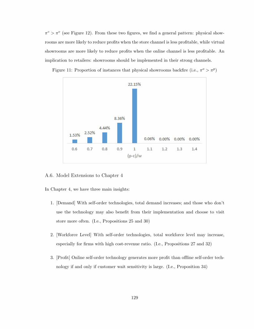
π◦ > πv (see Figure 12). From these two figures, we find a general pattern: physical show-
rooms are more likely to reduce profits when the store channel is less profitable, while virtual
showrooms are more likely to reduce profits when the online channel is less profitable. An
implication to retailers: showrooms should be implemented in their strong channels.
Figure 11: Proportion of instances that physical showrooms backfire (i.e., πo > πp)
A.6. Model Extensions to Chapter 4
In Chapter 4, we have three main insights:
1. [Demand] With self-order technologies, total demand increases; and those who don’t
use the technology may also benefit from their implementation and choose to visit
store more often. (I.e., Propositions 25 and 30)
2. [Workforce Level] With self-order technologies, total workforce level may increase,
especially for firms with high cost-revenue ratio. (I.e., Propositions 27 and 32)
3. [Profit] Online self-order technology generates more profit than offline self-order tech-
nology if and only if customer wait sensitivity is large. (I.e., Proposition 34)
129
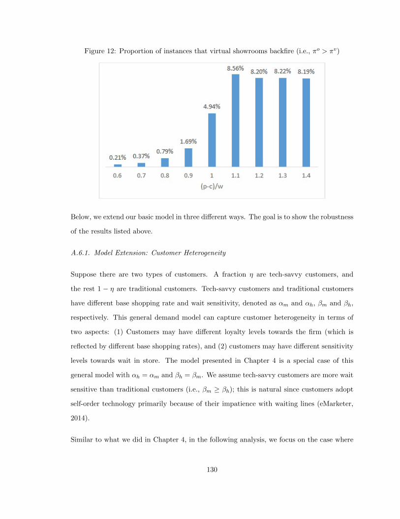
Figure 12: Proportion of instances that virtual showrooms backfire (i.e., πo > πv)
Below, we extend our basic model in three different ways. The goal is to show the robustness
of the results listed above.
A.6.1. Model Extension: Customer Heterogeneity
Suppose there are two types of customers. A fraction η are tech-savvy customers, and
the rest 1 − η are traditional customers. Tech-savvy customers and traditional customers
have different base shopping rate and wait sensitivity, denoted as αm and αh, βm and βh,
respectively. This general demand model can capture customer heterogeneity in terms of
two aspects: (1) Customers may have different loyalty levels towards the firm (which is
reflected by different base shopping rates), and (2) customers may have different sensitivity
levels towards wait in store. The model presented in Chapter 4 is a special case of this
general model with αh = αm and βh = βm. We assume tech-savvy customers are more wait
sensitive than traditional customers (i.e., βm ≥ βh); this is natural since customers adopt
self-order technology primarily because of their impatience with waiting lines (eMarketer,
2014).
Similar to what we did in Chapter 4, in the following analysis, we focus on the case where
130
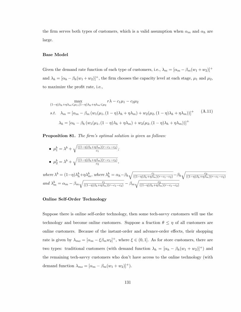
the firm serves both types of customers, which is a valid assumption when αm and αh are
large.
Base Model
Given the demand rate function of each type of customers, i.e., λm = [αm− βm(w1 +w2)]+
and λh = [αh−βh(w1 +w2)]+, the firm chooses the capacity level at each stage, µ1 and µ2,
to maximize the profit rate, i.e.,
max(1−η)λh+ηλm6µ1,(1−η)λh+ηλm6µ2
rλ− c1µ1 − c2µ2
s.t. λm = [αm − βm (w1(µ1, (1− η)λh + ηλm) + w2(µ2, (1− η)λh + ηλm))]+
λh = [αh − βh (w1(µ1, (1− η)λh + ηλm) + w2(µ2, (1− η)λh + ηλm))]+
(A.11)
Proposition 81. The firm’s optimal solution is given as follows:
• µb1 = λb +√
((1−η)βh+ηβm)(r−c1−c2)c1
;
• µb2 = λb +√
((1−η)βh+ηβm)(r−c1−c2)c2
,
where λb = (1−η)λbh+ηλbm, where λbh = αh−βh√
c1((1−η)βh+ηβm)(r−c1−c2)−βh
√c2
((1−η)βh+ηβm)(r−c1−c2)
and λbm = αm − βm√
c1((1−η)βh+ηβm)(r−c1−c2) − βm
√c2
((1−η)βh+ηβm)(r−c1−c2)
Online Self-Order Technology
Suppose there is online self-order technology, then some tech-savvy customers will use the
technology and become online customers. Suppose a fraction θ ≤ η of all customers are
online customers. Because of the instant-order and advance-order effects, their shopping
rate is given by λmo = [αm − ξβmw2]+, where ξ ∈ (0, 1]. As for store customers, there are
two types: traditional customers (with demand function λh = [αh − βh(w1 + w2)]+) and
the remaining tech-savvy customers who don’t have access to the online technology (with
demand function λms = [αm − βm(w1 + w2)]+).
131
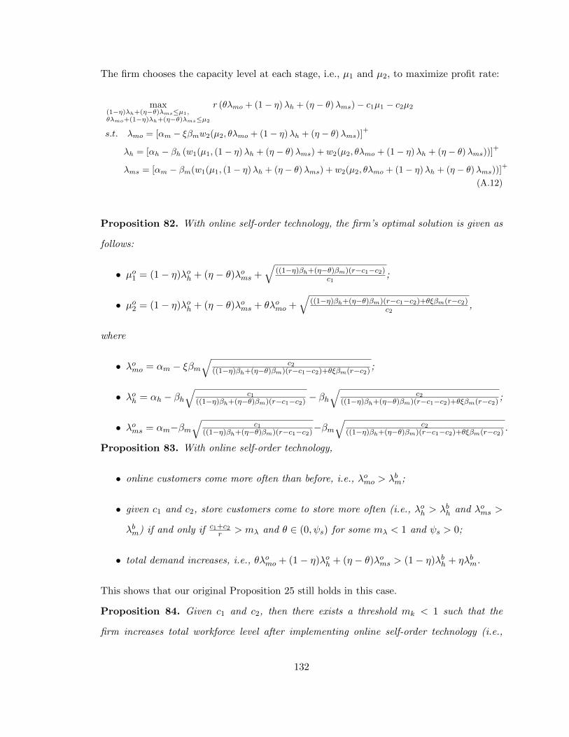
The firm chooses the capacity level at each stage, i.e., µ1 and µ2, to maximize profit rate:
max(1−η)λh+(η−θ)λms≤µ1,θλmo+(1−η)λh+(η−θ)λms≤µ2
r (θλmo + (1− η)λh + (η − θ)λms)− c1µ1 − c2µ2
s.t. λmo = [αm − ξβmw2(µ2, θλmo + (1− η)λh + (η − θ)λms)]+
λh = [αh − βh (w1(µ1, (1− η)λh + (η − θ)λms) + w2(µ2, θλmo + (1− η)λh + (η − θ)λms))]+
λms = [αm − βm(w1(µ1, (1− η)λh + (η − θ)λms) + w2(µ2, θλmo + (1− η)λh + (η − θ)λms))]+
(A.12)
Proposition 82. With online self-order technology, the firm’s optimal solution is given as
follows:
• µo1 = (1− η)λoh + (η − θ)λoms +√
((1−η)βh+(η−θ)βm)(r−c1−c2)c1
;
• µo2 = (1− η)λoh + (η − θ)λoms + θλomo +√
((1−η)βh+(η−θ)βm)(r−c1−c2)+θξβm(r−c2)c2
,
where
• λomo = αm − ξβm√
c2((1−η)βh+(η−θ)βm)(r−c1−c2)+θξβm(r−c2) ;
• λoh = αh − βh√
c1((1−η)βh+(η−θ)βm)(r−c1−c2) − βh
√c2
((1−η)βh+(η−θ)βm)(r−c1−c2)+θξβm(r−c2) ;
• λoms = αm−βm√
c1((1−η)βh+(η−θ)βm)(r−c1−c2)−βm
√c2
((1−η)βh+(η−θ)βm)(r−c1−c2)+θξβm(r−c2) .
Proposition 83. With online self-order technology,
• online customers come more often than before, i.e., λomo > λbm;
• given c1 and c2, store customers come to store more often (i.e., λoh > λbh and λoms >
λbm) if and only if c1+c2r > mλ and θ ∈ (0, ψs) for some mλ < 1 and ψs > 0;
• total demand increases, i.e., θλomo + (1− η)λoh + (η − θ)λoms > (1− η)λbh + ηλbm.
This shows that our original Proposition 25 still holds in this case.
Proposition 84. Given c1 and c2, then there exists a threshold mk < 1 such that the
firm increases total workforce level after implementing online self-order technology (i.e.,
132
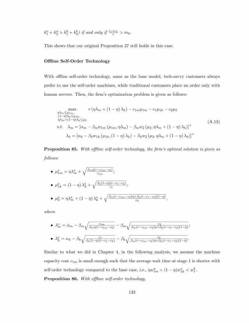
ko1 + ko2 > kb1 + kb2) if and only if c1+c2r > mk.
This shows that our original Proposition 27 still holds in this case.
Offline Self-Order Technology
With offline self-order technology, same as the base model, tech-savvy customers always
prefer to use the self-order machines, while traditional customers place an order only with
human servers. Then, the firm’s optimization problem is given as follows:
maxηλm≤µ1m,(1−η)λh≤µ1h,ηλm+(1−η)λh≤µ2
r (ηλm + (1− η)λh)− c1mµ1m − c1µ1h − c2µ2
s.t. λm = [αm − βmw1m (µ1m, ηλm)− βmw2 (µ2, ηλm + (1− η)λh)]+
λh = [αh − βhw1h (µ1h, (1− η)λh)− βhw2 (µ2, ηλm + (1− η)λh)]+
(A.13)
Proposition 85. With offline self-order technology, the firm’s optimal solution is given as
follows:
• µs1m = ηλsm +√
βmη(r−c1m−c2)c1m
;
• µs1h = (1− η)λsh +√
βh(1−η)(r−c1−c2)c1
;
• µs2 = ηλsm + (1− η)λsh +√
βm(r−c1m−c2)η+βh(r−c1−c2)(1−η)c2
,
where
• λsm = αm − βm√
c1mβmη(r−c1m−c2) − βm
√c2
βm(r−c1m−c2)η+βh(r−c1−c2)(1−η) ;
• λsh = αh − βh√
c1βh(1−η)(r−c1−c2) − βh
√c2
βm(r−c1m−c2)η+βh(r−c1−c2)(1−η) .
Similar to what we did in Chapter 4, in the following analysis, we assume the machine
capacity cost c1m is small enough such that the average wait time at stage 1 is shorter with
self-order technology compared to the base case, i.e., ηws1m + (1− η)ws1h < wb1.
Proposition 86. With offline self-order technology,
133
• tech-savvy customers come more often than before, i.e., λsm > λbm;
• given c1m, c1, c2, traditional customers come to store more often (i.e., λsh > λbh) if and
only if c1+c2r > m′λ and η ∈ (0, ψ′s) for some m′λ < 1 and ψ′s > 0;
• total demand increases, i.e., ηλsm + (1− η)λsh > (1− η)λbh + ηλbm.
This shows that our original Proposition 30 still holds in this case.
Proposition 87. Given c1m, c1 and c2, then there exists a threshold m′k < 1 such that
the firm increases total workforce level after implementing offline self-order technology (i.e.,
ks1 + ks2 > kb1 + kb2) if and only if c1+c2r > m′k.
This shows that our original Proposition 32 still holds in this case.
Profit Implications
Suppose βh = bbh and βm = bbm, i.e., b measures the base wait sensitivity in the market.
Proposition 88. There exists b ≥ 0 such that online self-order technology generates more
profit than offline self-order technology (i.e., πo > πs) if and only if b > b.
This shows that our original Proposition 34 still holds in this case.
A.6.2. Convex Impact of Wait Time
In Chapter 4, we assumed demand is a linear function of wait time. In this extension,
we relax this assumption. Specifically, we consider the following demand function: λ =
α−βwφ1 −βwφ2 , where w1 and w2 represent the wait times at stages 1 and 2, and parameter
φ ∈ (0, 1]. Since φ ∈ (0, 1], demand λ is convex with respect to wait time at each stage.
Note, the linear demand model presented in Chapter 4 is a special case of this general
demand model with φ = 1.
Similar to what we did in Chapter 4, in the following analysis, we focus on the case where
the firm serves all types of customers (including online, store, tech-savvy, traditional), which
134
is a valid assumption when α is large.
Base Model
Given the demand function, the firm chooses the capacity level at each stage, µ1 and µ2, to
maximize the profit rate, i.e.,
maxλ6µ1,λ6µ2
rλ− c1µ1 − c2µ2
s.t. λ =[α− β (w1(µ1, λ))φ − β (w2(µ2, λ))φ
]+(A.14)
Proposition 89. The firm’s optimal solution is given as follows:
• µb1 = λb +(φβ(r−c1−c2)
c1
) 11+φ
;
• µb2 = λb +(φβ(r−c1−c2)
c2
) 11+φ
,
where λb = α− β(
c1φβ(r−c1−c2)
) φ1+φ − β
(c2
φβ(r−c1−c2)
) φ1+φ
.
Online Self-Order Technology
With online self-order technology, because of the instant-order and advance-order effects,
online customer’s demand function is given as λo = α− ξβwφ2 . The store customer’s demand
function remains the same as before, i.e., λs = α − βwφ1 − βwφ2 . Therefore, the firm’s
optimization problem is as follows:
max(1−θ)λs≤µ1,(1−θ)λs+θλo≤µ2
r ((1− θ)λs + θλo)− c1µ1 − c2µ2
s.t. λo =[α− ξβ (w2(µ2, (1− θ)λs + θλo))
φ]+
λs =[α− β (w1(µ1, (1− θ)λs))φ − β (w2(µ2, (1− θ)λs + θλo))
φ]+
(A.15)
Proposition 90. With online self-order technology, the firm’s optimal solution is given as
follows:
135
• µo1 = (1− θ)λos +(φ(1−θ)β(r−c1−c2)
c1
) 11+φ
;
• µo2 = (1− θ)λos + θλoo +(φ(1−θ)β(r−c1−c2)+φθξβ(r−c2)
c2
) 11+φ
,
where
• λos = α− β(
c1φ(1−θ)β(r−c1−c2)
) φ1+φ − β
(c2
φ(1−θ)β(r−c1−c2)+φθξβ(r−c2)
) φ1+φ
,
• λoo = α− ξβ(
c2φ(1−θ)β(r−c1−c2)+φθξβ(r−c2)
) φ1+φ
.
Proposition 91. With online self-order technology,
• online customers come more often than before, i.e., λoo > λb;
• given c1 and c2, store customers come to store more often (i.e., λos > λb) if and only
if c1+c2r > mλ and θ ∈ (0, ψs) for some mλ < 1 and ψs > 0;
• total demand increases, i.e., (1− θ)λos + θλoo > λb.
This shows that our original Proposition 25 still holds in this case.
Proposition 92. Given c1 and c2, then there exists a threshold mk < 1 such that the
firm increases total workforce level after implementing online self-order technology (i.e.,
ko1 + ko2 > kb1 + kb2) if and only if c1+c2r > mk.
This shows that our original Proposition 27 still holds in this case.
Offline Self-Order Technology
With self-order technology, the firm’s optimization problem is given as follows:
maxηλm≤µ1m,(1−η)λh≤µ1hηλm+(1−η)λh≤µ2
r (ηλm + (1− η)λh)− c1mµ1m − c1µ1h − c2µ2
s.t. λm =[α− β(w1m (µ1m, ηλm))φ − β(w2 (µ2, ηλm + (1− η)λh))φ
]+
λh =[α− β(w1h (µ1h, (1− η)λh))φ − β(w2 (µ2, ηλm + (1− η)λh))φ
]+
(A.16)
136
Proposition 93. With offline self-order technology, the firm’s optimal solution is given as
follows:
• µs1m = ηλsm +(φβη(r−c1m−c2)
c1m
) 11+φ
;
• µs1h = (1− η)λsh +(φβ(1−η)(r−c1−c2)
c1
) 11+φ
;
• µs2 = ηλsm + (1− η)λsh +(φβη(r−c1m−c2)+φβ(1−η)(r−c1−c2)
c2
) 11+φ
,
where
• λsm = α− β(
c1mφβη(r−c1m−c2)
) φ1+φ − β
(c2
φβη(r−c1m−c2)+φβ(1−η)(r−c1−c2)
) φ1+φ
;
• λsh = α− β(
c1φβ(1−η)(r−c1−c2)
) φ1+φ − β
(c2
φβη(r−c1m−c2)+φβ(1−η)(r−c1−c2)
) φ1+φ
.
Similar to what we did in Chapter 4, in the following analysis, we assume the machine
capacity cost c1m is small enough such that the average wait time at stage 1 is shorter with
self-order technology compared to the base case, i.e., ηws1m + (1− η)ws1h < wb1.
Proposition 94. With offline self-order technology,
• tech-savvy customers come more often than before, i.e., λsm > λb;
• given c1m, c1, c2, traditional customers come to store more often (i.e., λsh > λb) if and
only if c1+c2r > m′λ and η ∈ (0, ψ′s) for some m′λ < 1) and ψ′s > 0;
• total demand increases, i.e., ηλsm + (1− η)λsh > λb.
This shows that our original Proposition 30 still holds in this case.
Proposition 95. Given c1m, c1 and c2, then there exists a threshold m′k < 1 such that
the firm increases total workforce level after implementing offline self-order technology (i.e.,
ks1 + ks2 > kb1 + kb2) if and only if c1+c2r > m′k.
This shows that our original Proposition 32 still holds in this case.
137
Profit Implications
Proposition 96. There exists β ≥ 0 such that online self-order technology generates more
profit than offline self-order technology (i.e., πo > πs) if and only if β > β.
This shows that our original Proposition 34 still holds in this case.
A.6.3. Alternative Wait Time Function
In Chapter 4, we formulated firm’s optimization problem with respect to capacity µ. The
three optimization problems (4.1, 4.2, 4.3) can also be reformulated with respect to the
number of servers k as follows:
• Basic model:
maxλ6k1/τ1,λ6k2/τ2
rλ− l1k1 − l2k2
s.t. λ = [α− β (w1(k1, λ) + w2(k2, λ))]+(4.1′)
• Online self-order technology:
max(1−θ)λs≤k1/τ1,θλo+(1−θ)λs≤k2/τ2
r (θλo + (1− θ)λs)− l1k1 − l2k2
s.t. λo = [α− ξβw2(k2, θλo + (1− θ)λs)]+
λs = [α− β (w1(k1, (1− θ)λs) + w2(k2, θλo + (1− θ)λs))]+
(4.2′)
• Offline self-order technology:
maxηλm≤k1m/τ1,(1−η)λh≤k1/τ1,ηλm+(1−η)λh≤k2/τ2
r (ηλm + (1− η)λh)− l1mk1m − l1k1 − l2k2
s.t. λm = [α− β (w1 (k1m, ηλm) + w2 (k2, ηλm + (1− η)λh))]+
λh = [α− β (w1 (k1, (1− η)λh) + w2 (k2, ηλm + (1− η)λh))]+
(4.3′)
138
where l1 = c1/τ1, l1m = c1m/τ1, l2 = c2/τ2, wi(k, λ) = 1k/τi−λ , and τi is the average service
time at stage i = 1, 2. Here, l1 and l2 can be interpreted as the labor cost per unit of time at
stages 1 and 2, l1m is the corresponding cost for machines. The number of machine servers
is denoted by k1m.
In Chapter 4, we have assumed wait time function takes the following form: wi(k, λ) =
1k/τi−λ . In this section, we numerically test the robustness of our main insights with a
different wait time function, i.e.,
wi(k, λ) =(τik
)ρ√2(k+1)−1
i
1− ρi
+ τi (A.17)
where ρi = λτik . This corresponds to the approximated average wait time in a M/M/k queue
(Cachon and Terwiesch, 2009).
In the numerical study, we consider the following parameter values:
• τ1 = {0.560 ,
160}. We assume the average service requirement is 0.5/60 or 1/60 hour
(i.e., 30 seconds or 1 min) to place an order.
• τ2 = tτ1, where t = {3, 5, 7}. Here, we only look at the case where τ2 > τ1 because it
generally takes longer cooking food at stage 2 than processing an order at stage 1.
• α = 100. Here, we assume the maximum traffic (i.e., if there is no wait) in a store is
100 people per hour.
• β = {300, 400, 500, 600}. This implies that the longest amount of wait time people
can tolerate (after which their shopping rate is 0) is α/β = {1/3, 1/4, 1/5, 1/6} hours.
• η = {0.6, 0.7, 0.8, 0.9}
• θ = ζη, where ζ = {0.2, 0.4, 0.6, 0.8}.
• ξ = {0.2, 0.4, 0.6, 0.8}
139
• l1 = l2 = {8, 9, 10, 11} The range of the hourly wage is consistent with the data
provided by the Bureau of Labor Statistics (http://www.bls.gov/oes/current/
oes353021.htm).
• l1m = xl1, where x = {0.01, 0.1}.
• l1τ1+l2τ2r = {0.1, 0.3, 0.5, 0.7}. The range of the cost-revenue ratio is selected based
on the following fact: According to National Restaurant Association (2010), for a
restaurant, the median cost of food and beverage sales is 31.9%, and the median cost
of salaries and wages is 29.4%. Note, l1τ1 + l2τ2 is the cost to serve one customer;
r is the sales revenue from each customer net of cost of food and beverage. Then,
the data above implies that the median of the cost-revenue ratio l1τ1+l2τ2r should be
around 29.4%/(1− 31.9%) = 43.2%.
There are 49.152 cases in total. After checking with the assumptions we made in Chapter 4,
we end up having 35,620 cases. For each case, we solve the three optimization problems
above with the wait time function (A.17). To simplify calculation, we assume k1, k2, k1m ∈
R+.
First, we check the impact of self-order technology on demand. Here are the results:
• With online technology, compared to the base scenario:
– total demand increases (i.e., θλoo + (1− θ)λos > λb) in all cases;
– online customers come more often (i.e., λoo > λb) in all cases;
– store customers come more often (i.e., λos > λb) in about 21.7% of cases.
• With offline technology, compared to the base scenario:
– total demand increases (i.e., ηλsm + (1− η)λsh > λb) in all cases;
– tech-savvy customers come more often (i.e., λsm > λb) in all cases;
140
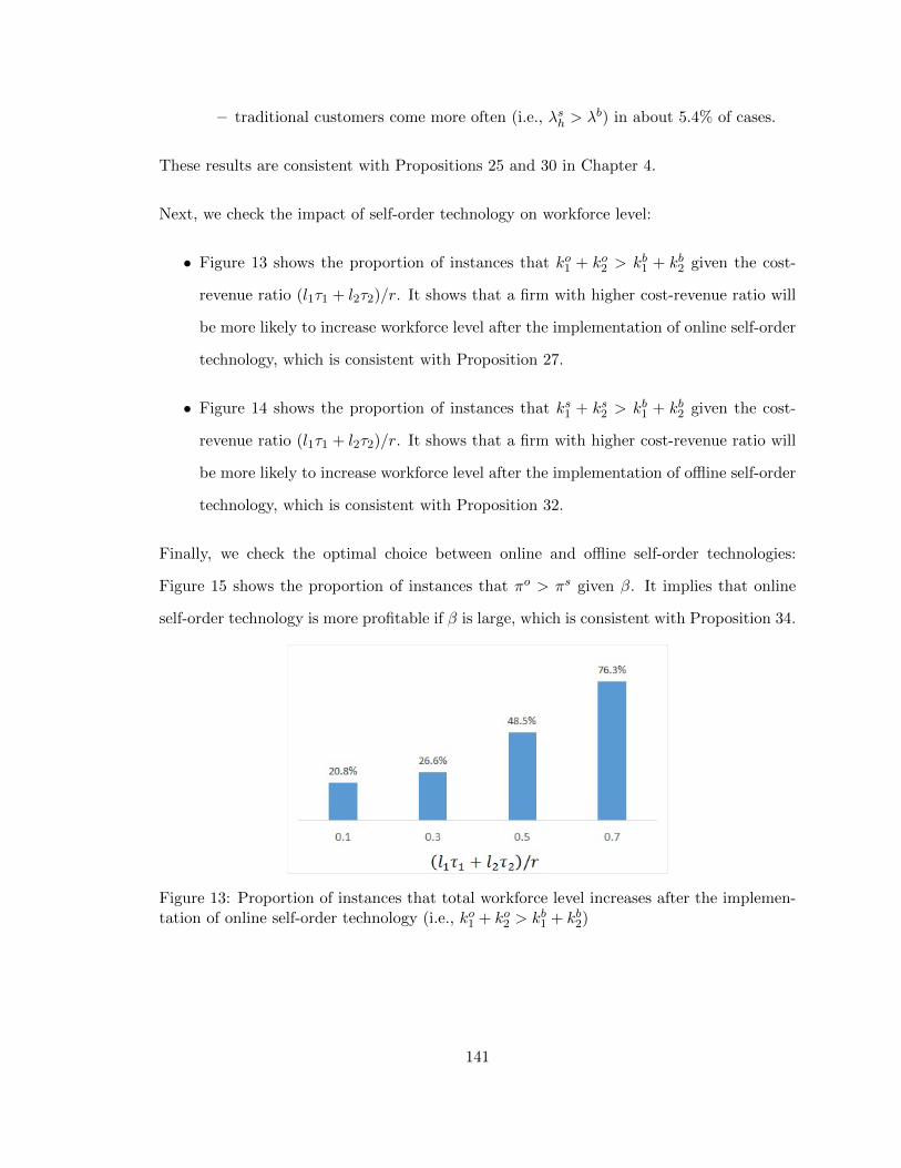
– traditional customers come more often (i.e., λsh > λb) in about 5.4% of cases.
These results are consistent with Propositions 25 and 30 in Chapter 4.
Next, we check the impact of self-order technology on workforce level:
• Figure 13 shows the proportion of instances that ko1 + ko2 > kb1 + kb2 given the cost-
revenue ratio (l1τ1 + l2τ2)/r. It shows that a firm with higher cost-revenue ratio will
be more likely to increase workforce level after the implementation of online self-order
technology, which is consistent with Proposition 27.
• Figure 14 shows the proportion of instances that ks1 + ks2 > kb1 + kb2 given the cost-
revenue ratio (l1τ1 + l2τ2)/r. It shows that a firm with higher cost-revenue ratio will
be more likely to increase workforce level after the implementation of offline self-order
technology, which is consistent with Proposition 32.
Finally, we check the optimal choice between online and offline self-order technologies:
Figure 15 shows the proportion of instances that πo > πs given β. It implies that online
self-order technology is more profitable if β is large, which is consistent with Proposition 34.
Figure 13: Proportion of instances that total workforce level increases after the implemen-tation of online self-order technology (i.e., ko1 + ko2 > kb1 + kb2)
141
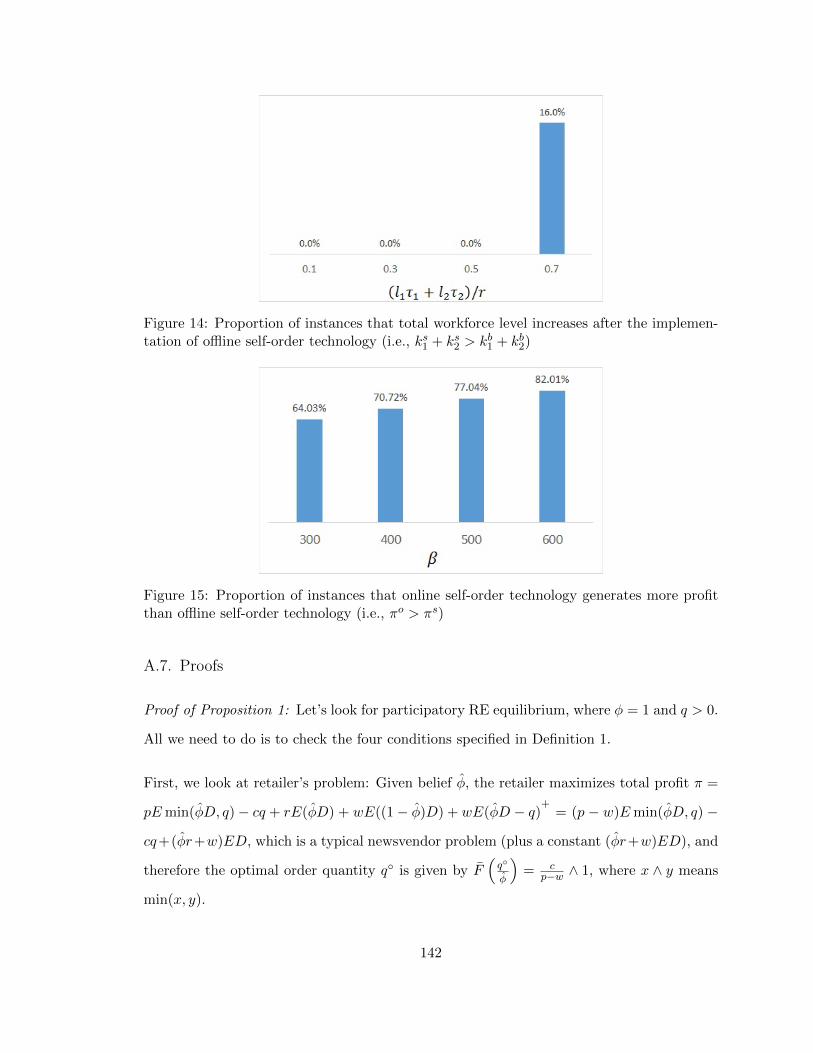
Figure 14: Proportion of instances that total workforce level increases after the implemen-tation of offline self-order technology (i.e., ks1 + ks2 > kb1 + kb2)
Figure 15: Proportion of instances that online self-order technology generates more profitthan offline self-order technology (i.e., πo > πs)
A.7. Proofs
Proof of Proposition 1: Let’s look for participatory RE equilibrium, where φ = 1 and q > 0.
All we need to do is to check the four conditions specified in Definition 1.
First, we look at retailer’s problem: Given belief φ, the retailer maximizes total profit π =
pEmin(φD, q)− cq + rE(φD) + wE((1− φ)D) + wE(φD − q)+= (p − w)Emin(φD, q) −
cq+(φr+w)ED, which is a typical newsvendor problem (plus a constant (φr+w)ED), and
therefore the optimal order quantity q◦ is given by F(q◦
φ
)= c
p−w ∧ 1, where x ∧ y means
min(x, y).
142
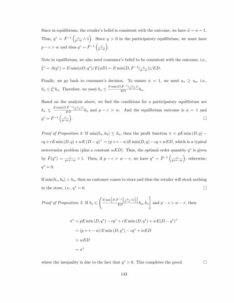
Since in equilibrium, the retailer’s belief is consistent with the outcome, we have φ = φ = 1.
Thus, q◦ = F−1(
cp−w ∧ 1
). Since q > 0 in the participatory equilibrium, we must have
p− c > w and thus q◦ = F−1(
cp−w
).
Note in equilibrium, we also need consumer’s belief to be consistent with the outcome, i.e.,
ξ◦ = A(q◦) = Emin(φD, q◦)/E(φD) = Emin(D, F−1( cp−w ))/ED.
Finally, we go back to consumer’s decision. To ensure φ = 1, we need us ≥ uo, i.e.,
hs ≤ ξ◦ho. Therefore, we need hs ≤Emin(D,F−1( c
p−w ))
ED ho.
Based on the analysis above, we find the conditions for a participatory equilibrium are
hs ≤Emin(D,F−1( c
p−w ))
ED ho and p − c > w. And the equilibrium outcome is φ = 1 and
q◦ = F−1(
cp−w
).
Proof of Proposition 2: If min(hs, hb) ≤ ho, then the profit function π = pEmin (D, q) −
cq+ rEmin (D, q) +wE (D − q)+ = (p+ r−w)Emin(D, q)− cq+wED, which is a typical
newsvendor problem (plus a constant wED). Thus, the optimal order quantity q∗ is given
by F (q∗) = cp+r−w ∧ 1. Then, if p − c > w − r, we have q∗ = F−1
(c
p+r−w
); otherwise,
q∗ = 0.
If min(hs, hb) > ho, then no customer comes to store and thus the retailer will stock nothing
in the store, i.e., q∗ = 0.
Proof of Proposition 3: If hs ∈
(Emin
[D,F−1
(c
p−w∧1)]
ED ho, ho
]and p− c > w − r, then
π∗ = pEmin (D, q∗)− cq∗ + rEmin (D, q∗) + wE(D − q∗)+
= (p+ r − w)Emin (D, q∗)− cq∗ + wED
> wED
= π◦
where the inequality is due to the fact that q∗ > 0. This completes the proof.
143
Proof of Proposition 4: If hb ≤ ho < hs and p − c > w − r, then q∗ = F−1(
cp+r−w
)> 0
because of Proposition 2. Then,
π∗ = pEmin (D, q∗)− cq∗ + rEmin (D, q∗) + wE(D − q∗)+
= (p+ r − w)Emin (D, q∗)− cq∗ + wED
> wED
= π◦
where the inequality is due to the fact that q∗ > 0. This completes the proof.
Proof of Proposition 5: If hs ≤Emin
(D,F−1
(c
p−w
))ED ho and p− c > w, we have q◦ 6= q∗ when
r > 0. Then
π◦ = pEmin (D, q◦)− cq◦ + rED + wE(D − q◦)+
= (p◦ − w)Emin (D, q◦)− cq◦ + rED + wED
> (p∗ − w)Emin (D, q∗)− cq∗ + rED + wED
> (p∗ − w)Emin (D, q∗)− cq∗ + rEmin (D, q∗) + wED
= p∗Emin (D, q∗)− cq∗ + rEmin (D, q∗) + wE(D − q∗)+
= π∗
where the first inequality is due to the strict concavity of the newsvendor profit function and
q◦ is the unique maximizer of π◦, and the second inequality is because ED > Emin(D, q)
for any q. This completes the proof.
Proof of Proposition 6: Note nonparticipatory equilibrium, (v−pH , 0, 0, 0, 0, 0, v−pH , 0, 0, 0), al-
ways exists. Same as what we did in the base model, we are going to look for participatory
equilibrium, where α◦s > 0, α◦so > 0 and q◦ > 0. All we need to do is to check the four
conditions specified in Definition 2.
First, we look at retailer’s problem: Given belief αo, αs, αso, the retailer maximizes total
144
profit
π = pEmin ((αs + αso)D, q)− cq + rE (αs + αso)D
+wEαoD + wE αsoαs+αso
((αs + αso)D − q)+
=(p− w αso
αs+αso
)Emin((αs + αso)D, q)− cq
+((αs + αso)r + (αo + αso)w)ED
which is a typical newsvendor problem (plus a constant ((αs + αso)r + (αo + αso)w)ED),
and therefore the optimal order quantity q◦ is given by F(
q◦
αs+αso
)= c
p−w αsoαs+αso
∧ 1.
Since in equilibrium, the retailer’s belief is consistent with the outcome, we have αi = α◦i ,
i = o, s, so. Note, in any participatory equilibrium, ξ > 0. Then, α◦soα◦s+α◦so
= v−p2H−(v−p) . Thus,
q◦ = (α◦s + α◦so)F−1
(c
p−w v−p2H−(v−p)
∧ 1
). Since q◦ > 0 in the participatory equilibrium, we
must have p− c > w v−p2H−(v−p) and thus q◦ = (α◦s + α◦so)F
−1
(c
p−w v−p2H−(v−p)
).
Note in equilibrium, we also need consumer’s belief to be consistent with the outcome, i.e.,
ξ = A(q◦) = Emin((α◦s + α◦so)D, q◦)/E((α◦s + α◦so)D) = Emin(D, F−1( c
p−w v−p2H−(v−p)
))/ED,
which is indeed greater than 0. Thus, there are customers who are willing to come to store.
Based on the analysis above, we find the condition for a participatory equilibrium is p−c >
w v−p2H−(v−p) . And the equilibrium store inventory level q◦ = F−1
(c
p−w v−p2H−(v−p)
).
Proof of Proposition 7: Note the retailer’s profit can be expressed as
π =(p+ r − w α∗so+α
∗bo
α∗s+α∗b+α∗so+α∗bo
)Emin ((α∗s + α∗b + α∗so + α∗bo)D, q)− cq
+w(α∗o + α∗so + α∗bo)ED
which is a typical newsvendor problem (plus a constant w(α∗o + α∗so + α∗bo)ED). Thus, the
optimal store inventory level is given by
q∗ = (α∗s + α∗b + α∗so + α∗bo) F−1
c
p+ r − w α∗so+α∗bo
α∗s+α∗b+α∗so+α∗bo
∧ 1
145
Proof of Proposition 8: Denote A◦l = {(hs, ho)|max(v − p − ho,−hs + ξ◦(v − p)) < 0} and
A∗l = {(hs, ho)|max(v − p − ho, v − p − hs, v − p − βshs − βoho) < 0}. To prove part (i),
we simply need to show that A∗l ⊂ A◦l . Since ξ◦ < 1, for any (hs, ho) ∈ A∗l , we will have
(hs, ho) ∈ A◦l . Thus, A∗l ⊂ A◦l .
Next, let’s look at part (ii). To simplify notation, we denote ∆◦ = v−p2H−(v−p) and ∆∗ =
α∗so+α∗bo
α∗s+α∗b+α∗so+α∗bo
. Note if βs + βo > 1, we have ∆◦ < ∆∗. Thus, p−c∆◦ >
p−c∆∗ .
If there are customers visiting store when there is no BOPS, we need to have w < p−c∆◦ . The
following analysis assumes this condition holds.
Suppose r = 0. If w ≥ p−c∆∗ (this is possible since p−c
∆◦ > p−c∆∗ ), then no one comes to store
when there is BOPS . In this case,
π∗ = wE (α∗so + α∗bo + α∗o)D
= wE (α◦so + α◦o)D
< pEmin ((α◦s + α◦so)D, q)− cq + rE (α◦s + α◦so)D + wEα◦oD
+ wEα◦so
α◦s + α◦so((α◦s + α◦so)D − q)
+
= π◦
where the inequality is because q = 0 is also a feasible but not the optimal solution to the
case where there is no BOPS. If w < p−c∆∗ , then there are consumers visiting store when
there is BOPS. Note (1) π◦ − π∗ is continuous in w, and (2) π◦ > π∗ when w = p−c∆∗ . Thus,
the analysis above implies that there exists w < p−c∆∗ such that π◦ > π∗ if w > w.
Proof of Proposition 9: Note πs is a typical newsvendor profit function. Then, the optimal
order quantity q∗ is given by F (q∗) = cθp+r ∧ 1. Thus, if θp + r − c > 0, we have q∗ =
F−1(
cθp+r
), otherwise, q∗ = 0.
146
Proof of Proposition 10: In the decentralized system, for any θ, denote optimal stock levels
in the store as q∗(θ). Suppose we have the same stock level in the centralized system. Then
clearly we will achieve exactly the same total profit as π∗(θ), since the BOPS revenue is
just shared between channels in the decentralized case. Thus, we must have π∗(θ) ≤ π∗.
And due to the fact that π is strictly concave in q and q∗ > 0 (because of the assumptions
that hb < min(hs, ho) and p− c > w − r), we have π∗(θ) = π∗ if only if q∗ = q∗.
Next, let’s compare the optimal store inventory levels in both the centralized and decen-
tralized systems:
• If θ < p−wp , then c
θp+r >c
p+r−w . Thus, q∗ = F−1(
cθp+r
)< F−1
(c
p+r−w
)= q∗. Since
q∗ 6= q∗, π∗ < π∗.
• If θ = p−wp , then c
θp+r = cp+r−w . Thus, q∗ = F−1
(c
θp+r
)= F−1
(c
p+r−w
)= q∗. Since
q∗ = q∗, π∗ = π∗.
• If θ > p−wp , then c
θp+r <c
p+r−w . Thus, q∗ = F−1(
cθp+r
)> F−1
(c
p+r−w
)= q∗. Since
q∗ 6= q∗, π∗ < π∗.
Finally, let’s prove π∗ is quasiconcave in θ.
Let’s first show that π∗ is nondecreasing in θ < p−wp . If θ ≤ c−r
p , then q∗ = 0 and thus
π∗ = wED, which is independent of θ. If θ ∈ ( c−rp , p−wp ), then ∂π∗
∂θ = ∂π∗
∂q∂q∗
∂θ > 0, because
∂π∗
∂q > 0 if q < q∗ and ∂q∗
∂θ > 0.
Then, let’s show that π∗ is nonincreasing in θ > p−wp . Note ∂π∗
∂θ = ∂π∗
∂q∂q∗
∂θ < 0, because
∂π∗
∂q < 0 if q > q∗ and ∂q∗
∂θ > 0.
Thus, we can conclude that π∗ is quasiconcave in θ.
Proof of Proposition 35: Note πs is a typical newsvendor profit function. Then, the optimal
order quantity q∗ is given by F ( q∗
α∗s+α∗b+α∗so+α∗bo
) = c(α∗s+α∗so
α∗s+α∗b
+α∗so+α∗bo
+α∗b
+α∗bo
α∗s+α∗b
+α∗so+α∗boθ
)p+r∧ 1.
147
Thus, if(α∗s+α∗so
α∗s+α∗b+α∗so+α∗bo
+α∗b+α∗bo
α∗s+α∗b+α∗so+α∗boθ)p+ r − c > 0, then
q∗ = (α∗s + α∗b + α∗so + α∗bo) F−1
c(α∗s+α∗so
α∗s+α∗b
+α∗so+α∗bo
+α∗b
+α∗bo
α∗s+α∗b
+α∗so+α∗boθ
)p+r
, otherwise, q∗ = 0.
Proof of Proposition 11: Let’s look for participatory RE equilibrium, where φ = 1. All we
need to do is to check the four conditions specified in Definition 1.
First, we look at the retailer’s problem: Note the profit function can be expressed as
π = (p−w+ r 1−θθ )Emin(φθD, q)− cq+ (wθ− r(1− θ))ED, which is a typical newsvendor
problem (plus a constant (wθ + r(1− θ))ED), and therefore the optimal order quantity q◦
is given by F(q◦
φθ
)= c
p−w+r 1−θθ
.
Since in equilibrium, the retailer’s belief is consistent with the outcome, we have φ = φ = 1.
Thus, q◦ = θF−1
(c
p−w+r 1−θθ
).
Note in equilibrium, we also need consumer’s belief to be consistent with the outcome, i.e.,
ξ◦ = A(q◦) = Emin(φθD, q◦)/E(φθD) = Emin(D, F−1( cp−w+r 1−θ
θ
))/ED.
Finally, we need to check, given ξ = Emin(D, F−1( cp−w+r 1−θ
θ
))/ED, consumers are indeed
willing to visit store, i.e., us > uo, which gives us the condition
hs <Emin(D, F−1( c
p−w+r 1−θθ
))
ED[ho + (1− θ)hr]. (SA.1)
Note the right hand side of condition (SA.1) is decreasing in θ and is also boundless for
θ ∈ R. Therefore, there exists a unique θ◦ ∈ R such that hs =Emin(D,F−1( c
p−w+r 1−θ◦θ◦
))
ED [ho +
(1− θ◦)hr] and condition (SA.1) is equivalent to θ < θ◦. Since θ ∈ (0, 1) in our model, we
truncate the cutoff point and set ψ◦ = min(max(θ◦, 0), 1).
Based on the analysis above, we find the condition for a participatory equilibrium is θ < ψ◦.
148
In such case, the equilibrium store inventory level is q◦ = θF−1
(c
p−w+r 1−θθ
), which is
strictly positive, since condition (SA.1) will not hold otherwise.
Proof of Proposition 12: Let’s look for participatory RE equilibrium, where φ = 1.
First, we look at the retailer’s problem: Note the profit function can be expressed as
π = (p−w)Emin(φθD, q)− cq + (wθ− r(1− φ)(1− θ))ED, which is a typical newsvendor
problem (plus a constant (wθ−r(1−φ)(1−θ))ED), and therefore the optimal order quantity
qp is given by F(qp
φθ
)= c
p−w .
Since in equilibrium, the retailer’s belief is consistent with the outcome, we have φ = φ = 1.
Thus, qp = θF−1(
cp−w
).
Note in equilibrium, we also need consumer’s belief to be consistent with the outcome, i.e.,
ξp = A(qp) = Emin(φθD, qp)/E(φθD) = Emin(D, F−1( cp−w ))/ED.
Finally, we need to check given ξ = Emin(D, F−1( cp−w ))/ED, consumers are indeed willing
to visit store, i.e., us > uo, which gives us the condition
hs <Emin(D, F−1( c
p−w ))
EDθho + (1− θ)(ho + hr). (SA.2)
Note the left hand side of condition (SA.2) is decreasing in θ and is also boundless for θ ∈ R.
Therefore, there exists a unique θp ∈ R such that hs =Emin(D,F−1( c
p−w ))
ED θpho+(1−θp)(ho+
hr) and condition (SA.2) is equivalent to θ < θp. Since θ ∈ (0, 1) in our model, we truncate
the cutoff point and set ψp = min(max(θp, 0), 1) and thus we get the equilibrium result.
Note ∂ψo
∂r ≥ 0 and ∂ψp
∂r = 0. Also, when r = 0, condition (SA.1) implies condition (SA.2),
and thus θp ≥ θ◦ or ψp ≥ ψ◦. Therefore, ∃r ≥ 0 such that ψp > ψ◦ if and only if r < r.
149
Proof of Proposition 13: If θ < ψp, then we have
π◦ = pEmin(θD, q◦)− cq◦ + wE(θD − q◦)+ − rE 1− θθ
(θD − q◦)+
< pEmin(θD, q◦)− cq◦ + wE(θD − q◦)+
< pEmin(θD, qp)− cqp + wE(θD − qp)+ = πp
where the second inequality is because qp rather than q◦ is the optimal solution that maxi-
mizes the newsvendor profit function πp.
If ψp < ψ◦ and θ ∈ [ψp, ψ◦), then we have
π◦ = pEmin(θD, q◦)− cq◦ + wE(θD − q◦)+ − rE 1− θθ
(θD − q◦)+
= (p− w − r1− θθ
)Emin(θD, q◦)− cq◦ + wθED − rE(1− θ)D
> wEθD − rE(1− θ)D = πp
If θ ≥ max(ψp, ψ◦), then π◦ = wEθD − rE(1− θ)D = πp.
Proof of Proposition 14: Since this is just the base model with a new set of parameter θ′
and D′, similar to the proof of Proposition 1, we can show that the participatory equilibrium
exists if and only if
hs <
Emin(D′, F ′−1( c
p−w+r 1−θ′θ′
))
ED′[ho + (1− θ′)hr]. (SA.3)
and in the participatory equilibrium, we have φv = 1 and qv = θ′F ′( c
p−w+r 1−θ′θ′
) > 0.
Since D′ = [1 − α(1 − θ)]D and F ′(x) = F ( x1−α(1−θ)), the right hand side of condi-
tion (SA.3) equals to
Emin
(D,F−1
(c
p−w+r 1−θ′θ′
))ED [ho + (1 − θ′)hr], which is decreasing in
θ and is also boundless for θ ∈ R. Therefore, there exists a unique θv ∈ R such that
hs =
Emin(D,F−1( c
p−w+r1−θ′(θv)θ′(θv)
))
ED [ho + (1 − θ′(θv))hr] and condition (SA.3) is equivalent
to θ < θv, where θ′(θv) = θv
1−α(1−θv) , i.e., the posterior fraction of high-type customers
150
given prior θv. Since θ ∈ (0, 1) in our model, we truncate the cutoff point and set
ψv = min(max(θv, 0), 1) and thus we get the equilibrium result.
Since θ′ > θ, it is easy to show that condition (SA.3) implies condition (SA.1), and thus
θ◦ ≥ θv. Therefore, their truncated counterparts ψ◦ ≥ ψv.
Proof of Proposition 15: If θ < ψv, then we have
π◦ = pEmin(θD, q◦)− cq◦ + wE(θD − q◦)+ − rE 1− θθ
(θD − q◦)+
< pEmin(θD, q◦)− cq◦ + wE(θD − q◦)+ − rE 1− θ′
θ′(θD − q◦)+
= pEmin(θ′D′, q◦)− cq◦ + wE(θ′D′ − q◦)+ − rE 1− θ′
θ′(θ′D′ − q◦)+
< pEmin(θ′D′, qv)− cqv + wE(θ′D′ − qv)+ − rE 1− θ′
θ′(θ′D′ − qv)+ = πv
where the first inequality is because of θ′ > θ, the second inequality is because qv rather
than q◦ is the optimal solution that maximizes the newsvendor profit function πv.
If θ ≥ ψ◦, then we have π◦ = wEθD − rE(1 − θ)D < wEθD − rE(1 − α)(1 − θ)D =
wEθ′D′ − r(1− θ′)D′ = πv.
If θ ∈ [ψv, ψ◦), then π◦ = (p − w + r 1−θθ )Emin(θD, q◦) − cq◦ + (wθ − r(1 − θ))ED, while
πv = wEθ′D′ − rE(1− θ′)D′ = wEθD − rE(1− α)(1− θ)D. Then, by Envelop Theorem,
∂(π◦−πv)∂w = ∂π◦
∂w −∂πv
∂w = −Emin(θD, q◦) < 0. To conclude the result, we just need to note
that it is indeed possible to have π◦ > πv, e.g., when α is very close to 0.
Proof of Proposition 16: Comparing us,in and uo, we have
• us,in > uo if the following condition holds
hs < ho + (1− θ)hr (SA.4)
Then, consumers visit store if store is in stock. Thus, retailer profit function is π =
151
pEmin(θD, q)−cq+wE(θD−q)+−rE 1−θθ (θD−q)+ = (p−w+r 1−θ
θ )Emin(θD, q)−
cq+(wθ−r(1−θ))ED, which is a typical newsvendor problem (plus a constant (wθ+
r(1−θ))ED), and therefore the optimal order quantity qa = θF−1
(c
p−w+r 1−θθ
). Note
condition (SA.4) is equivalent to θ < ψa, where ψa = min(max(ho+hr−hshr, 0), 1), given
θ ∈ (0, 1). Moreover, note if the critical fractile cp−w+r 1−θ
θ
≥ 1 (⇔ θ ≥ r(w+r−p+c)+ ,
given θ ∈ (0, 1)), then qa = 0, i.e., store is never in stock and thus consumers actually
always buy online as a result.
• If condition (SA.4) does not hold, i.e., θ ≥ ψa, then us,in ≤ uo and consumers buy
online directly. Then, it is easy to see that the optimal store inventory level is qa = 0.
By setting ψa = min( r(w+r−p+c)+ , ψ
a), we get the market outcome.
Finally, to prove ψa ≥ ψ◦, we only need to note the following two facts: First, since
condition (SA.1) implies condition (SA.4), we have ψa ≥ ψ◦; second, since cp−w+r 1−θ
θ
≥ 1
(or θ ≥ r(w+r−p+c)+ ) implies that q◦ = 0, we have r
(w+r−p+c)+ ≥ ψ◦.
Proof of Proposition 17: If θ < ψ◦, then we have
π◦ = pEmin(θD, q◦)− cq◦ + wE(θD − q◦)+ − rE 1− θθ
(θD − q◦)+
= pEmin(θD, qa)− cqa + wE(θD − qa)+ − rE 1− θθ
(θD − qa)+ = πa
If θ ≥ ψa, then we have π◦ = wEθD − rE(1− θ)D = πa.
If θ ∈ [ψ◦, ψa), then we have
π◦ = wEθD − rE(1− θ)D
< (p− w + r1− θθ
)Emin(θD, qa)− cqa + wEθD − rE(1− θ)D
= pEmin(θD, qa)− cqa + wE(θD − qa)+ − rE 1− θθ
(θD − qa)+ = πa
152
Proof of Proposition 18: First, note condition A.3 in Appendix A.3.1 implies condition (SA.2),
thus ψpa ≤ ψp. Moreover, it is easy to check that ψpa
= ψa. Since ψpa ≤ ψpa
, we have
ψpa ≤ ψa.
1. If θ < ψpa, then πp = pEmin (θD, qp) − cqp + wE(θD − qp)+ = pEmin (θD, qpa) −
cqpa + wE(θD − qpa)+ = πpa and
πp = pEmin (θD, qp)− cqp + wE(θD − qp)+
> pEmin (θD, qa)− cqa + wE(θD − qa)+
> pEmin (θD, qa)− cqa + wE(θD − qa)+ − rE 1− θθ
(θD − qa)+ = πa
where the first inequality is because qp is the unique maximal of πp. Thus, we have
πp = πpa > πa.
2. If θ ∈ [ψpa,min(ψp, ψa)), then
πp = pEmin (θD, qp)− cqp + wE(θD − qp)+
> pEmin (θD, qa)− cqa + wE(θD − qa)+
> pEmin (θD, qa)− cqa + wE(θD − qa)+ − rE 1− θθ
(θD − qa)+ = πa
and
πa = pEmin (θD, qa)− cqa + wE(θD − qa)+ − rE 1− θθ
(θD − qa)+
= pEmin (θD, qpa)− cqpa + wE(θD − qpa)+ − rE 1− θθ
(θD − qpa)+ = πpa
Thus, we have πp > πa = πpa
3. If θ ∈ [min(ψp, ψa),max(ψp, ψa)),
153
• if ψp < ψa, then
πa = pEmin (θD, qa)− cqa + wE(θD − qa)+ − rE 1− θθ
(θD − qa)+
= pEmin (θD, qpa)− cqpa + wE(θD − qpa)+ − rE 1− θθ
(θD − qpa)+ = πpa
and
πa = pEmin (θD, qa)− cqa + wE(θD − qa)+ − rE 1− θθ
(θD − qa)+
=
(p− w + r
1− θθ
)Emin (θD, qa)− cqa + wEθD − rE (1− θ)D
> wEθD − rE (1− θ)D = πp
Thus, we have πa = πpa > πp;
• if ψp > ψa, then
πa = pEmin (θD, qa)− cqa + wE(θD − qa)+ − rE 1− θθ
(θD − qa)+
= pEmin (θD, qpa)− cqpa + wE(θD − qpa)+ − rE 1− θθ
(θD − qpa)+ = πpa
and
πp = pEmin (θD, qp)− cqp + wE(θD − qp)+
> pEmin (θD, qa)− cqa + wE(θD − qa)+
> pEmin (θD, qa)− cqa + wE(θD − qa)+ − rE 1− θθ
(θD − qa)+ = πa
Thus, we have πp > πa = πpa.
4. If θ ≥ max(ψp, ψa), then πp = πa = πpa = wEθD − rE(1− θ)D.
Proof of Proposition 19: The addition of virtual showrooms only creates a new customer
pool with D′ and θ′. Then since ψp is determined by condition (SA.2), ψpv should be
154
determined by condition hs <Emin(D′,F
′−1( cp−w ))
ED′ θho + (1 − θ′)(ho + hr), which is implied
by condition (SA.2). Thus, we have ψpv ≤ ψp.
If θ < ψpv, then πp = pEmin (θD, qp)− cqp +wE(θD − qp)+ = pEmin (θ′D′, qpv)− cqpv +
wE(θ′D′ − qpv)+ = πpv and
πp = pEmin (θD, qp)− cqp + wE(θD − qp)+
> max(pEmin (θD, qv)− cqv + wE(θD − qv)+, wEθD
)> max
(pEmin
(θ′D′, qv
)− cqv + wE
(θ′D′ − qv
)+ − rE 1− θ′
θ′(θ′D′ − qv
)+,
wEθ′D′ − rE(1− θ′
)D′
)
= πv
If θ ∈ [ψpv, ψp), then πp = pEmin (θD, qp)−cqp+wE(θD − qp)+ = (p− w)Emin (θD, qp)−
cqp + wEθD > wEθ′D′ − rE (1− θ′)D = πpv and
πp = pEmin (θD, qp)− cqp + wE(θD − qp)+
> max(pEmin (θD, qv)− cqv + wE(θD − qv)+, wEθD
)> max
(pEmin
(θ′D′, qv
)− cqv + wE
(θ′D′ − qv
)+ − rE 1− θ′
θ′(θ′D′ − qv
)+,
wEθ′D′ − rE(1− θ′
)D′
)
= πv
If θ ∈ [ψp,max(ψp, ψv)), then πp = wEθD − rE(1− θ)D and πpv = wEθ′D′ − r(1− θ′)D′,
155
and
πv = pEmin(θ′D′, qv
)− cqv + wE
(θ′D′ − qv
)+ − rE 1− θ′
θ′(θ′D′ − qv
)+=
(p− w + r
1− θ′
θ′
)Emin
(θ′D′, qv
)− cqv + wEθ′D′ − rE
(1− θ′
)D′
> wEθ′D′ − rE(1− θ′
)D′
= wEθD − r (1− α)E (1− θ)D
≥ max (πpv, πp)
If θ ≥ max(ψp, ψv), πv = πpv = wEθ′D′ − r(1 − θ′)D′ = wEθD − r (1− α)E (1− θ)D >
wEθD − rE(1− θ)D = πp.
Proof of Proposition 20: Let’s first prove the part (i):
Think of the case with virtual showroom as a new base model with a new customer pool.
Then, since ψa ≥ ψ◦, we should also have ψva ≥ ψv.
If θ ∈ [ψv, ψva), then
πva = pEmin(θ′D′, qva
)− cqva + wE
(θ′D′ − qva
)+ − rE 1− θ′
θ′(θ′D′ − qva
)+=
(p− w + r
1− θ′
θ′
)Emin
(θ′D′, qva
)− cqva + wEθ′D′ − rE
(1− θ′
)D′
> wEθ′D′ − rE(1− θ′
)D′ = πv
and
πva = pEmin(θ′D′, qva
)− cqva + wE
(θ′D′ − qva
)+ − rE 1− θ′
θ′(θ′D′ − qva
)+> pEmin
(θ′D′, qa
)− cqa + wE
(θ′D′ − qa
)+ − rE 1− θ′
θ′(θ′D′ − qa
)+> pEmin (θD, qa)− cqa + wE(θD − qa)+ − rE 1− θ
θ(θD − qa)+ = πa
156
Thus, we get part (i).
Next, let’s look at part (ii):
Since we can think of the case with virtual showroom as a new base model with new
customer pool (θ′ and D′), the proof should be similar to the proof of Proposition 18 and
thus omitted.
Proof of Proposition 21: Let’s first look at the case when θ < ψp. In Proposition 13, we
have shown that πp > π◦. Thus, all we need to show is that physical showroom is strictly
better than the other three options as well.
πp = pEmin (θD, qp)− cqp + wE(θD − qp)+
> max(pEmin (θD, qv)− cqv + wE(θD − qv)+, wEθD
)> max
(pEmin
(θ′D′, qv
)− cqv + wE
(θ′D′ − qv
)+ − rE 1− θ′
θ′(θ′D′ − qv
)+,
wEθ′D′ − rE(1− θ′
)D′
)
= πv
A similar argument could be used to prove πp > πva, by simply replacing the superscript
·v with ·va in the equation above. Finally, compared with the case where there is only
availability information
πp = pEmin (θD, qp)− cqp + wE(θD − qp)+
> max(pEmin (θD, qa)− cqa + wE(θD − qa)
+, wEθD
)> max
(pEmin (θD, qa)− cqa + wE(θD − qa)
+ − rE 1− θθ
(θD − qa)+, wEθD − rE (1− θ)D
)= πa
So, we can conclude π∗ = πp.
157
Next, let’s look at the case where θ ≥ ψp. Let’s first show the suboptimality of the option
of offering only physical showroom:
• if θ < max(ψp, ψ◦), then
π◦ = pEmin (θD, q◦)− cq◦ + wE(θD − q◦)+ − rE 1− θθ
(θD − q◦)+
=
(p− w + r
1− θθ
)Emin (θD, q◦)− cq◦ + wEθD − rE (1− θ)D
> wEθD − rE (1− θ)D = πp
• if θ > max(ψp, ψ◦), then π◦ = wEθD − rE (1− θ)D = πp
So in the following analysis, we only need to look at the other four types of information.
• Case 1: θ < ψ◦. Note that if ψp ≥ ψ◦, we don’t even have this case. So in the
following proof, we only focus on the case when ψp < ψ◦. Note when α = 0, we have
ψv = ψ◦ and ψva = ψa. Also, it is easy to check that ∂ψv
∂α ≤ 0 and ∂ψva
∂α ≤ 0. Then,
let’s set α1 = arg minα∈[0,1]
|θ − ψv (α)| and α2 = arg minα∈[0,1]
|θ − ψva (α)|. Since ∀α ψv ≤ ψva,
we have α1 ≤ α2.
– If α < α1, then θ < ψv ≤ min(ψ◦, ψva) ≤ ψa. Therefore, πv = πva and πa = π◦.
Moreover,
πv = pEmin(θ′D′, qv
)− cqv + wE
(θ′D′ − qv
)+ − rE 1− θ′
θ′(θ′D′ − qv
)+> pEmin
(θ′D′, qa
)− cqa + wE
(θ′D′ − qa
)+ − rE 1− θ′
θ′(θ′D′ − qa
)+> pEmin (θD, qa)− cqa + wE(θD − qa)+ − rE 1− θ
θ(θD − qa)+ = πa
Thus, π∗ = πv.
158
– If α ∈ (α1, α2), then ψv < θ < min(ψ◦, ψva) ≤ πa. Therefore, πa = π◦. Also,
πva = pEmin(θ′D′, qva
)− cqva + wE
(θ′D′ − qva
)+ − rE 1− θ′
θ′(θ′D′ − qva
)+> pEmin
(θ′D′, qa
)− cqa + wE
(θ′D′ − qa
)+ − rE 1− θ′
θ′(θ′D′ − qa
)+> pEmin (θD, qa)− cqa + wE(θD − qa)+ − rE 1− θ
θ(θD − qa)+ = πa
and
πva = pEmin(θ′D′, qva
)− cqva + wE
(θ′D′ − qva
)+ − rE 1− θ′
θ′(θ′D′ − qva
)+=
(p− w + r
1− θ′
θ′
)Emin
(θ′D′, qva
)− cqva + wEθ′D′ − rE
(1− θ′
)D′
> wEθ′D′ − rE(1− θ′
)D′ = πv
Thus, we can conclude π∗ = πva.
– If α > α2, then ψv ≤ ψva < θ < ψ◦ ≤ ψa. Therefore, πa = π◦ and πv = πva.
Thus, we only need to compare π◦ and πv. Because ∂(πv−π◦)∂α = r(1− θ)ED > 0,
there exists α3 ≥ α2 such that π◦ > πv if and only if α ∈ (α2, α3). Thus, π∗ = π◦
if α ∈ (α2, α3); π∗ = πv if α > α3.
• Case 2: θ > ψ◦.
– If θ ∈ [max(ψ◦, ψp),max(ψa, ψp)], then let’s set α′1 = arg minα∈[0,1]
|θ − ψva (α)|.
∗ If α < α′1, then ψv ≤ ψ◦ < θ < ψva ≤ ψa. Therefore, πv = wEθ′D′− rE(1−
θ′)D′ > wEθD − r(1− θ)D = π◦. Also,
πva = pEmin(θ′D′, qva
)− cqva + wE
(θ′D′ − qva
)+ − rE 1− θ′
θ′(θ′D′ − qva
)+> pEmin
(θ′D′, qa
)− cqa + wE
(θ′D′ − qa
)+ − rE 1− θ′
θ′(θ′D′ − qa
)+> pEmin (θD, qa)− cqa + wE(θD − qa)+ − rE 1− θ
θ(θD − qa)+ = πa
159
and
πva = pEmin(θ′D′, qva
)− cqva + wE
(θ′D′ − qva
)+ − rE 1− θ′
θ′(θ′D′ − qva
)+=
(p− w + r
1− θ′
θ′
)Emin
(θ′D′, qva
)− cqva + wEθ′D′ − rE
(1− θ′
)D′
> wEθ′D′ − rE(1− θ′
)D′ = πv
Thus, we can conclude π∗ = πva.
∗ If α > α′, then ψv ≤ min(ψ◦, πva) ≤ max(ψ◦, ψva) < θ < ψa. Therefore,
πva = πv and
πa = pEmin (θD, qa)− cqa + wE(θD − qa)+ − rE 1− θθ
(θD − qa)+
=
(p− w + r
1− θθ
)Emin (θD, qa)− cqa + wEθD − rE (1− θ)D
> wEθD − rE (1− θ)D = π◦
Thus, we conly need to compare πv and πa. Because ∂(πv−πa)∂α = r(1 −
θ)ED > 0, there exists α′2 ≥ α′1 such that πa > πv if and only if α ∈ (α′1, α′2).
Thus π∗ = πa if α ∈ (α′1, α′2); π∗ = πv if α > α′2.
– If θ > max(ψa, ψp), then since ψv ≤ ψ◦ and ψa ≥ ψ◦, we have ψa ≥ ψv.
Also, note ψa is determined by condition (SA.4), which is implied by condition
hs < ho+(1−θ′)hr, which could be shown to determine the cutoff ψva. Thus, we
also have ψva ≤ ψa. Then, if θ ≥ max(ψp, ψa), we have πv = πva = wEθ′D′ −
rE(1 − θ′)D′ > wEθD − rE(1 − θ)D = πa = πp = π◦. So we can conclude
π∗ = πv. In this case, we can simply set α′1 = α′2 = 0.
160
Proof of Proposition 22: First, consider the following optimization problem:
max0≤λ≤µ1≤ rαc1 ,0≤λ≤µ2≤ rαc2
rλ− c1µ1 − c2µ2
s.t. λ = α− β (w1(µ1, λ) + w2(µ2, λ))
(A.18)
Since the constraint set is compact and the objective function is continuous, by Weierstass
Theorem, there is a maximum to (A.18). Let’s denote the optimal solution to (A.18) as
λ∗, µ∗1, µ∗2, then the corresponding optimal objective value π∗ = rλ∗ − c1µ
∗1 − c2µ
∗2.
Lemma 2. If π∗ > 0, then (λ∗, µ∗1, µ∗2) must be the optimal solution to the optimization
problem (4.1); if π∗ ≤ 0, then there is no solution to (4.1) that yields positive profit.
Proof of Lemma 2: If π∗ > 0, then we must have λ∗ > 0. Thus, (λ∗, µ∗1, µ∗2) is also a feasible
solution to (1). Suppose the optimal solution to (1) is (λb, µb1, µb2) 6= (λ∗, µ∗1, µ
∗2). Then, it
means that πb = rλb − c1µb1 − c2µ
b2 > π∗ > 0. Then, it is easy to check that (λb, µb1, µ
b2) is
a feasible solution to (A.18) as well. But it leads to a higher objective value πb for (A.18),
which contradicts to the fact that (λ∗, µ∗1, µ∗2) is the optimal solution to (A.18). Thus, we
must have (λb, µb1, µb2) = (λ∗, µ∗1, µ
∗2).
If π∗ ≤ 0, suppose there exists a solution (λb, µb1, µb2) to (1) such that πb = rλb−c1µ
b1−c2µ
b2 >
0. Then, it is easy to check that (λb, µb1, µb2) should also be a feasible solution to (A.18),
which leads to a positive objective value πb for (A.18). This contradicts to the fact that
π∗ ≤ 0. Thus, there is no solution to (4.1) that yields positive profit.
By Lemma 2, finding the optimal solution to (4.1) that yields positive profit is equivalent
to finding the optimal solution to (A.18) that yields positive profit.
The Lagrangian of (A.18) is defined as follows:
L (λ, µ1, µ2, ρ) = rλ− c1µ1 − c2µ2 + ρ
[λ− α+ β
(1
µ1 − λ+
1
µ2 − λ
)]
161
where ρ ∈ R is the Lagrange multiplier. To find the critical points of L (λ, µ1, µ2, ρ), we
solve the following equation set:
∂L∂λ = r + ρ+ ρβ 1
(µ1−λ)2 + ρβ 1(µ2−λ)2 = 0
∂L∂µi
= −ci − ρβ 1(µi−λ)2 = 0, i = 1, 2
λ− α+ β(
1µ1−λ + 1
µ2−λ
)= 0
0 ≤ λ ≤ µ1 ≤ rαc1, 0 ≤ λ ≤ µ2 ≤ rα
c2
By Proposition 5.6 in (Sundaram, 1996)[page 122], we know the optimal solution to (A.18)
is one of the critical points. (Note the constraint qualification holds everywhere on the
feasible set.) Let’s first ignore the boundary conditions that 0 ≤ λ and µi ≤ rαci
, and solve
the equation set above, which gives us a unique solution:
λ∗ = α− β√
c1β(r−c1−c2) − β
√c2
β(r−c1−c2)
µ∗1 = λ∗ +√
β(r−c1−c2)c1
µ∗2 = λ∗ +√
β(r−c1−c2)c2
(A.19)
So, if λ∗ ≥ 0 and µ∗i ≤ rαci
, i = 1, 2, then (λ∗, µ∗1, µ∗2) must be the optimal solution to
(A.18); otherwise, the optimal solution to (A.18) must be corner solution (i.e., at least one
of the follow holds, λ∗ = 0 and µ∗i = rαci
, i = 1, 2), in which case the optimal value is clearly
nonpositive. Note, with (λ∗, µ∗1, µ∗2) defined in (A.19), we have π∗ = rλ∗−c1µ
∗1−c2µ
∗2 = (r−
c1− c2)α−2√β(r − c1 − c2)c1−2
√β(r − c1 − c2)c2, which is positive if α >
2√β(√c1+√c2)√
r−c1−c2.
It is easy to check that if α >2√β(√c1+√c2)√
r−c1−c2, we have λ∗ ≥ 0 and µ∗i ≤ rα
ci, i = 1, 2. This
implies that there is an optimal solution (λ∗, µ∗1, µ∗2) that yields positive profit for (A.18) if
and only if α > α =2√β(√c1+√c2)√
r−c1−c2. Then, by Lemma 2, we can conclude that same result
holds for the optimization problem (4.1).
Proof of Proposition 23: Suppose we set the two capacity levels at µb1, µb2 (i.e., the optimal
162
solution in the base model). Then, the demand rates are
λ?o =[α− ξβw2(µb2, (1− θ)λ?s + θλ?o)
]+λ?s =
[α− β
(w1(µb1, (1− θ)λ?s) + w2(µb2, (1− θ)λ?s + θλ?o)
)]+It is easy to check (1− θ)λ?s + θλ?o > λb. This implies that the profit with µb1, µ
b2 and online
self-order technology is greater than πb. Therefore, under optimal solution, there must be
customers coming to store after the implementation of online self-order technology, i.e., at
least one of λos and λoo is positive. Note, if λos > 0, we must have λoo > 0. Thus, we must
have λoo > 0 in the optimal solution. So the optimization problem (4.2) is equivalent to the
following problem
max0≤λo,(1−θ)λs≤µ1,(1−θ)λs+θλo≤µ2
r ((1− θ)λs + θλo)− c1µ1 − c2µ2
s.t. λo = α− ξβw2(µ2, (1− θ)λs + θλo)
λs = [α− β (w1(µ1, (1− θ)λs) + w2(µ2, (1− θ)λs + θλo))]+
(A.20)
Then, the firm has two choices:
i. Shut down stage 1 (i.e., µ1 = 0) and sell only to online customers. In this case, the
optimal solution is obtained by solving the following optimization problem:
max0≤λo,θλo≤µ2≤ rαc2
rθλo − c2µ2
s.t. λo = α− ξβw2(µ2, θλo)
(A.21)
The Lagrangian of (A.21) is defined as follows:
L (λo, µ2, ρ) = rθλo − c2µ2 + ρ
[λo − α+ ξβ
1
µ2 − θλo
]
where ρ ∈ R is the Lagrange multiplier. To find the critical points of L (λo, µ2, ρ), we
163
solve the following equation set:
∂L∂λo
= rθ + ρ+ ρξβθ 1(µ2−θλo)2 = 0
∂L∂µ2
= −c2 − ρξβ 1(µ2−θλo)2 = 0
λo − α+ ξβ 1µ2−θλo = 0
0 ≤ λo, θλo ≤ µ2 ≤ rαc2
By Proposition 5.6 in (Sundaram, 1996)[page 122], we know the optimal solution to
(A.21) is one of the critical points. (Note the constraint qualification holds everywhere
on the feasible set.) Let’s first ignore the conditions that 0 ≤ λo and µ2 ≤ rαc2
, and
solve the equation set above, which gives us a unique solution:
λ∗o = α− ξβ√
c2θξβ(r−c2)
µ∗2 = λ∗o +√
θξβ(r−c2)c2
(A.22)
So, if λ∗ ≥ 0 and µ∗2 ≤ rαc2
, then (λ∗o, µ∗2) together with λ∗1 = 0, µ∗1 = 0 must be the
optimal solution to (A.21); otherwise, the optimal solution to (A.21) must be corner
solution (i.e., at least one of the follow holds, λ∗o = 0 and µ∗2 = rαc2
), in which case the
optimal value is clearly nonpositive, and thus the firm won’t choose this option at all.
ii. Sell to both types of customers. In this case, the optimal solution is obtained by
solving the following optimization problem:
max0≤λo,0≤(1−θ)λs≤µ1≤ rαc1 ,(1−θ)λs+θλo≤µ2≤ rαc2
r ((1− θ)λs + θλo)− c1µ1 − c2µ2
s.t. λo = α− ξβw2(µ2, (1− θ)λs + θλo)
λs = α− β (w1(µ1, (1− θ)λs) + w2(µ2, (1− θ)λs + θλo))
(A.23)
164
The Lagrangian of (A.23) is defined as follows:
L (λs, λo, µ1, µ2, ρ1, ρ2) =r ((1− θ)λs + θλo)− c1µ1 − c2µ2
+ ρ1
[λo − α+ ξβ
1
µ2 − (1− θ)λs − θλo
]+ ρ2
[λs − α+ β
1
µ1 − (1− θ)λs+ β
1
µ2 − (1− θ)λs − θλo
]
where ρ1, ρ2 ∈ R are the Lagrange multipliers. To find the critical points of
L (λs, λo, µ1, µ2, ρ1, ρ2), we solve the following equation set:
∂L∂λs
= r (1− θ) + ρ2 + ρ1ξβ (1− θ) 1(µ2−(1−θ)λs−θλo)2 + ρ2β (1− θ) 1
(µ1−(1−θ)λs)2
+ρ2β (1− θ) 1(µ2−(1−θ)λs−θλo)2 = 0
∂L∂λo
= rθ + ρ1 + ρ1ξβθ1
(µ2−(1−θ)λs−θλo)2 + ρ2βθ1
(µ2−(1−θ)λs−θλo)2 = 0
∂L∂µ1
= −c1 − ρ2β1
(µ1−(1−θ)λs)2 = 0
∂L∂µ2
= −c2 − ρ1ξβ1
(µ2−(1−θ)λs−θλo)2 − ρ2β1
(µ2−(1−θ)λs−θλo)2 = 0
λo − α+ ξβ 1µ2−(1−θ)λs−θλo = 0
λs − α+ β 1µ1−(1−θ)λs + β 1
µ2−(1−θ)λs−θλo = 0
0 ≤ λo, 0 ≤ (1− θ)λs ≤ µ1 ≤ rαc1, (1− θ)λs + θλo ≤ µ2 ≤ rα
c2
By Proposition 5.6 in (Sundaram, 1996)[page 122], we know the optimal solution to
(A.23) is one of the critical points. (Note the constraint qualification holds everywhere
on the feasible set.) Let’s first ignore the boundary conditions (i.e., 0 ≤ λo, 0 ≤ λs
and µi ≤ rαci
i = 1, 2), and solve the equation set above, which gives us a unique
solution:
λ∗s = α− β√
c1(1−θ)β(r−c1−c2) − β
√c2
(1−θ)β(r−c1−c2)+θξβ(r−c2)
λ∗o = α− ξβ√
c2(1−θ)β(r−c1−c2)+θξβ(r−c2)
µ∗1 = (1− θ)λos +√
(1−θ)β(r−c1−c2)c1
µ∗2 = (1− θ)λos + θλoo +√
(1−θ)β(r−c1−c2)+θξβ(r−c2)c2
So, if (λ∗o, λ∗s, µ∗1, µ∗2) is an interior solution, then it must be the optimal solution to
165
(A.23); otherwise, the solution to (A.23) must be corner solution, in which case we can
check the optimal value is either nonpositive or strictly less than that under option
(i), and thus the firm never chooses this option.
Therefore, the optimal solution to (A.20) (and thus to (4.2)) must be chosen from the
interior solutions under the two options, whichever gives higher optimal value. For option
(i), under the interior solution (λ∗o, λ∗s, µ∗1, µ∗2), the optimal value is π∗ = r((1−θ)λ∗s+θλ∗o)−
c1µ∗1 − c2µ
∗2 = (r − c2)θα − 2
√θξβ(r − c2)c2; for option (ii), under the interior solution
(λ∗o, λ∗s, µ∗1, µ∗2), the optimal value is π∗ = r((1− θ)λ∗s + θλ∗o)− c1µ
∗1− c2µ
∗2 = (r− c2− c1(1−
θ))α− 2√
(1− θ)β(r − c1 − c2)c1 − 2√
[(1− θ)β(r − c1 − c2) + θξβ(r − c2)]c2. Thus, π∗ <
π∗ if and only if α > α′′ = 2√βc1√
(1−θ)(r−c1−c2)+
2√
[(1−θ)β(r−c1−c2)+θξβ(r−c2)]c2(r−c1−c2)(1−θ) − 2
√θξβ(r−c2)c2
(r−c1−c2)(1−θ) .
Then, we conclude the proof by setting α′ = max(α, α′′).
Proof of Proposition 24: From Propositions 22 and 23, we get wb1 =√
c1β(r−c1−c2) , wb2 =√
c2β(r−c1−c2) , wo1 =
√c1
(1−θ)β(r−c1−c2) , and wo2 =√
c2(1−θ)β(r−c1−c2)+θξβ(r−c2) . Since θ > 0, we
have wo1 > wb1. Also, note that∂(wo2−wb2)
∂r > 0 and limr→c1+c2
(wo2 − wb2
)< 0. Thus, given c1
and c2, ∃r > c1 + c2 such that wo2 < wb2 if and only if c1+c2r > c1+c2
r = mw.
Proof of Proposition 25: λoo = α−√
ξ2β2c2(1−θ)β(r−c1−c2)+θξβ(r−c2) ≥ α−
√βc2
(1−θ)(r−c1−c2)+θ(r−c2) >
α −√
βc2r−c1−c2 > α −
√βc1
r−c1−c2 −√
βc2r−c1−c2 = λb where the first inequality is because of
ξ ≤ 1.
Next, let’s prove the second bullet point in Proposition 25. Note,
(λos − λbs
) √r − c1 − c2
β=
√c1
β+
√c2
β−√
c1
(1− θ)β−√
c2
(1− θ)β + θξβ r−c2r−c1−c2
which is decreasing in r for r ≥ c1 + c2. When r → c1 + c2,(λos − λbs
) √r−c1−c2β →
√c1β +√
c2β −
√c1
(1−θ)β > 0 if θ < ψs = 1−( √
c1√c1+√c2
)2. Then, we can conclude the result.
166
By Proposition 24, λos > λb must happen when wo2 < wb2, and thus we have mλ > mw.
Finally, let’s prove the third point in Proposition 25. Note (1− θ)λos+θλoo = α−√
(1−θ)βc1r−c1−c2 −
√c2√
(1−θ)β+θξβ√r− (1−θ)β(c1+c2)+θξβc2
(1−θ)β+θξβ
. Also,∂√
(1−θ)βc1∂θ < 0,
∂√
(1−θ)β+θξβ
∂θ ≤ 0, and∂
(1−θ)β(c1+c2)+θξβc2(1−θ)β+θξβ
∂θ < 0.
Thus, (1− θ)λos + θλoo is increasing in θ. Note when θ = 0, we have (1− θ)λos + θλoo = λb.
Thus, (1− θ)λos + θλoo > λb for all θ > 0.
Proof of Proposition 26: Note µo1 =√
1− θ
(√
1− θα−√
βc1r−c1−c2−
√βc2
(r−c1−c2)+θ/(1−θ)ξ(r−c2)+
√β(r−c1−c2)
c1
), which is decreasing in θ. Since when θ = 0 we have µo1 = µb1, we can conclude
µo1 < µb1 for any θ > 0.
Next, let’s prove part (ii). Note that
µo2−µb2√β(r−c1−c2)
=√c1−√
(1−θ)c1r−c1−c2 +
√c2−(1−θ+θξ)
√c2
1−θ+θξ r−c2r−c1−c2
r−c1−c2
+
√1−θ+θξ r−c2
r−c1−c2c2
−√
1c2
(A.24)
It is easy to find the 1st and 3rd terms in (A.24) are decreasing in r. Also, since ξ ≤ 1,
we have√c2 − (1− θ + θξ)
√c2
1−θ+θξ r−c2r−c1−c2
> 0. Thus, we find the 2nd term in (A.24)
is also decreasing in r. In sum, we findµo2−µb2√β(r−c1−c2)
is decreasing in r. Note, when
−β (r − c1 − c2) + ξβ (r − c2) = 0 (i.e., r = c1+c2−ξc21−ξ > c1 + c2). then µo2 − µb2
=(1−√
1− θ)√ βc1
r−c1−c2 + (1− ξ) θ√
βc2r−c1−c2 > 0. Thus, there exists r > c1+c2−ξc2
1−ξ such
that µo2 > µb2 if and only if r < r. Then, we can define mµ = c1+c2r and conclude the result.
Because (1−θ)λos+θλoo > λb, wo2 < wb2 implies µo2 > µb2. Thus, we must have mµ < mw.
167
Proof of Proposition 27:
ko1 + ko2 − kb1 − kb2 = −θατ1 +√
βc1r−c1−c2 (τ1 + τ2)
(1−√
1− θ)
− (τ1 + τ2)
[((1− θ)β + θξβ)
√c2
(1−θ)β(r−c1−c2)+θξβ(r−c2) − β√
c2β(r−c1−c2)
]−√
β(r−c1−c2)c1
τ1
(1−√
1− θ)
+τ2
(√(1−θ)β(r−c1−c2)+θξβ(r−c2)
c2−√
β(r−c1−c2)c2
)+τ1θξβ
√c2
(1−θ)β(r−c1−c2)+θξβ(r−c2)
(A.25)
Let’s first show the 3rd term in (A.25), i.e.,
− (τ1 + τ2)
[((1− θ)β + θξβ)
√c2
(1−θ)β(r−c1−c2)+θξβ(r−c2)−β√
c2β(r−c1−c2)
](denoted as f3(r))
is decreasing in r:
∂f3
∂r= − (τ1 + τ2)
−√c2
2
√(1− θ)β + θξβ(
r − c2 − (1−θ)βc1(1−θ)β+θξβ
) 32
+
√βc2
2(r − c1 − c2)32
Since ∂[(1−θ)β+θξβ]∂θ ≤ 0 and
∂[r−c2− (1−θ)βc1(1−θ)β+θξβ
]
∂θ > 0, we can find that ∂f3
∂r is decreasing in θ.
Note when θ = 0, ∂f3
∂r = 0. Thus, ∂f3
∂r < 0 for all θ > 0.
Next, let’s show the 5th term in (A.25), i.e., τ2
(√(1−θ)β(r−c1−c2)+θξβ(r−c2)
c2−√
β(r−c1−c2)c2
)(denoted as f5(r)) is decreasing in r: Note,
∂√
(1−θ)β(r−c1−c2)+θξβ(r−c2)
∂r =
√(1−θ)β+θξβ
2√r− (1−θ)β(c1+c2)+θξβc2
(1−θ)β+θξβ
.
Since∂√
(1−θ)β+θξβ
∂θ ≤ 0 and∂
(1−θ)β(c1+c2)+θξβc2(1−θ)β+θξβ
∂θ < 0, we find∂√
(1−θ)β(r−c1−c2)+θξβ(r−c2)
∂r is
decreasing in θ, and thus ∂f5
∂r is decreasing in θ. Note when θ = 0, we have ∂f5
∂r = 0. Thus,
∂f5
∂r < 0 for all θ > 0.
Therefore, we can conclude that∂(ko1+ko2−kb1−kb2)
∂r < 0. Note, if r → c1 + c2, we have (ko1 +
ko2−kb1−kb2)√r − c1 − c2 → (τ1 +τ2)
√βc2 +
√βc1(τ1 +τ2)(1−
√(1− θ)) > 0, which implies
ko1 + ko2 − kb1 − kb2 > 0 if r is very close to c1 + c2. Thus, there exists r > c1 + c2 such that
ko1 + ko2 − kb1 − kb2 > 0 if and only if r < r. Then, we can define mk = c1+c2r . Since to have
ko1 + ko2 − kb1 − kb2 > 0, we must have µo2 > µb2, this implies mk > mµ.
168
Proof of Proposition 28: The retailer has three options to choose from:
1. Serve only tech savvy customers (i.e., by setting µ1h = 0), and the optimization
problem is
max0≤ηλm≤µ1m≤ rα
c1m0≤ηλm≤µ2≤ rαc2
rηλm − c1mµ1m − c2µ2
s.t.λm = α− β 1µ1m−ηλm − β
1µ2−ηλm
if we ignore the boundary conditions, we can derive the unique optimal solution as
λ∗m = α− β√
c1mηβ(r−c1m−c2) − β
√c2
ηβ(r−c1m−c2)
µ∗1m = ηλ∗m +√
ηβ(r−c1m−c2)c1m
µ∗2 = ηλ∗m +√
ηβ(r−c1m−c2)c2
(A.26)
and the corresponding optimal value is π∗ = (r−c1m−c2)ηα−2√ηβ(r − c1m − c2)c1m−
2√ηβ(r − c1m − c2)c2. So, if (λ∗m, µ
∗1m, µ
∗2) is an interior solution, then it must be the
optimal solution to (A.26); otherwise, the solution to (A.26) must be corner solution,
in which case we can check the optimal value is clearly nonpositive, and thus the firm
never chooses this option.
2. Serve only traditional customers (i.e., by setting µ1m = 0), and the optimization
problem is
max0≤(1−η)λh≤µ1h≤ rαc10≤(1−η)λh≤µ2≤ rαc2
r (1− η)λh − c1hµ1h − c2µ2
s.t. λh = α− β 1µ1h−(1−η)λh
− β 1µ2−(1−η)λh
(A.27)
if we ignore the boundary conditions, we can derive the unique optimal solution as
λ∗h = α− β√
c1(1−η)β(r−c1−c2) − β
√c2
(1−η)β(r−c1−c2)
µ∗1 = (1− η)λ∗m +√
(1−η)β(r−c1−c2)c1
µ∗2 = (1− η)λ∗m +√
(1−η)β(r−c1−c2)c2
and the corresponding optimal value is π∗ = (r − c1 − c2)(1− η)α
169
− 2√
(1− η)β(r − c1 − c2)c1 − 2√
(1− η)β(r − c1 − c2)c2. So, if (λ∗h, µ∗1, µ∗2) is an
interior solution, then it must be the optimal solution to (A.27); otherwise, the solution
to (A.27) must be corner solution, in which case we can check the optimal value is
clearly nonpositive, and thus the firm never chooses this option.
3. Serve both types of customers. In this case, the optimal solution is obtained by solving
the following optimization problem:
max0≤ηλm≤µ1m≤ rα
c1m,
0≤(1−η)λh≤µ1h≤ rαc1 ,ηλm+(1−η)λh≤µ2≤ rαc2
r (ηλm + (1− η)λh)− c1mµ1m − c1µ1h − c2µ2
s.t. λm = α− βw1m (µ1m, ηλm)− βw2 (µ2, ηλm + (1− η)λh)
λh = α− βw1h (µ1h, (1− η)λh)− βw2 (µ2, ηλm + (1− η)λh)
(A.28)
Since the constraint set is compact and the objective function is continuous, by Weier-
strass Theorem, there is a maximum to (A.28).
The Lagrangian of (A.28) is defined as follows:
L(λm, λh, µ1m, µ1h, µ2, ρm, ρh) = r (ηλm + (1− η)λh)− c1mµ1m − c1µ1h − c2µ2
−ρm(λm − α+ β 1
µ1m−ηλm + β 1µ2−ηλm−(1−η)λh
)−ρh
(λh − α+ β 1
µ1h−(1−η)λh+ β 1
µ2−ηλm−(1−η)λh
)where ρm, ρh ∈ R are the Lagrange multiplier. To find the critical points of
L(λm, λh, µ1m, µ1h, µ2, ρm, ρh), we solve the following equation set:
∂L∂λm
= rη − ρm − ρmβη
(µ1m−ηλm)2 − (ρm+ρh)βη
(µ2−ηλm−(1−η)λh)2 = 0
∂L∂λh
= r (1− η)− ρh − ρhβ(1−η)
(µ1h−(1−η)λh)2 − (ρm+ρh)β(1−η)
(µ2−ηλm−(1−η)λh)2 = 0
∂L∂µ1m
= −c1m + ρmβ
(µ1m−ηλm)2 = 0
∂L∂µ1h
= −c1 + ρhβ(1−η)
(µ1h−(1−η)λh)2 = 0
∂L∂µ2
= −c2 + (ρm+ρh)β(1−η)
(µ2−ηλm−(1−η)λh)2 = 0
0 ≤ ηλm ≤ µ1m ≤ rαc1m
, 0 ≤ (1− η)λh ≤ µ1h ≤ rαc1, ηλm + (1− η)λh ≤ µ2 ≤ rα
c2
170
By Proposition 5.6 in (Sundaram, 1996)[page 122], we know the optimal solution to
(A.28) is one of the critical points. (Note the constraint qualification holds everywhere
on the feasible set.) Let’s first ignore the boundary conditions, and solve the equation
set above, which gives us a unique solution:
λ∗m = α− β√
c1mβη(r−c1m−c2) − β
√c2
β[(r−c1m−c2)η+(r−c1−c2)(1−η)]
λ∗h = α− β√
c1β(1−η)(r−c1−c2) − β
√c2
β[(r−c1m−c2)η+(r−c1−c2)(1−η)]
µ∗1m = ηλ∗m +√
βη(r−c1m−c2)c1m
µ∗1h = (1− η)λ∗h +√
β(1−η)(r−c1−c2)c1
µ∗2 = ηλ∗m + (1− η)λ∗h +√
β[(r−c1m−c2)η+(r−c1−c2)(1−η)]c2
Note it is easy to check that if λ∗m ≥ 0 and λ∗h ≥ 0, then µi ≤ rαci
. Thus, if λ∗m ≥ 0 and
λ∗h ≥ 0 (or α is large), then (λ∗m, λ∗h, µ∗1m, µ
∗1h, µ
∗2) is the optimal solution to (A.28),
and the corresponding optimal value is π∗ = (r− c1m− c2)ηα+ (r− c1− c2)(1−η)α−
2√ηβc1m(r − c1m − c2)− 2
√(1− η)β(r − c1 − c2)c1
− 2√βc2[(r − c1m − c2)η + (r − c1 − c2)(1− η)].
So, if (λ∗m, λ∗h, µ∗1m, µ
∗1h, µ
∗2) is an interior solution, then it must be the optimal solution
to (A.28); otherwise, the solution to (A.28) must be corner solution, in which case we
can check the optimal value is either nonpositive or strictly less than that under the
first two options, and thus the firm never chooses this option.
Note π∗ − π∗ and π∗ − π∗ are linearly increasing in α, and thus if and only if α is large
enough, we have π∗ > max(π∗, π∗), and thus it is optimal for the firm to serve both types
of customers.
Proof of Lemma 1: From the optimal solution given in Proposition 28, we know ws1h =√c1
β(1−η)(r−c1−c2) , ws1m =√
c1mβη(r−c1m−c2) , and ws2 =
√c2
β[(r−c1m−c2)η+(r−c1−c2)(1−η)] .
171
Then, ηws1m + (1− η)ws1h =√
ηc1mβ(r−c1m−c2) +
√(1−η)c1
β(r−c1−c2) which is increasing in c1m. Also,
when c1m = 0, ηws1m + (1− η)ws1h < wb1. Thus, there exists c1m > 0 such that ηws1m + (1−
η)ws1h < wb1 if and only if c1m < c1m.
Proof of Proposition 29: Because η < 1, we can find ws1h > wb1. Since ηws1m + (1− η)ws1h <
wb1, we must have ws1m < wb1. Also, since c1m < c1, we have ws2 < wb2.
Proof of Proposition 30: First, because ws1m < wb1 and ws2 < wb2, we find λsm = α− βws1m −
βws2 > α− βwb1 − βwb2 = λb.
Second, note
(λsh − λb
)√r − c1 − c2
β=
√c1
β+
√c2
β−√
c1
β (1− η)−√
c2
βη r−c1m−c2r−c1−c2 + β (1− η)
which is decreasing in r. Then, if limr→c1+c2
(λsh−λb)√r−c1−c2
β =√
c1β +
√c2β −
√c1
β(1−η) > 0
(i.e., η is small enough), then there exists r > c1 + c2 such that λsh > λb if and only if r < r
(or c1+c2r < c1+c2
r = m′λ).
Finally, note
ηλsm + (1− η)λsh = α−√
ηβc1m
r − c1m − c2−
√(1− η)βc1
r − c1 − c2
−
√βc2
(r − c1m − c2) η + (r − c1 − c2) (1− η)
> α−√
βc1
r − c1 − c2−
√βc2
(r − c1 − c2)
= λb
where the inequality is due to c1m < c1 and Assumption 1, which implies ηws1m+(1−η)ws1h <
wb1 (by Lemma 1) or√
ηβc1mr−c1m−c2 +
√(1−η)βc1r−c1−c2 <
√βc1
r−c1−c2 ).
172
Proof of Proposition 31: Note µs1h =√
1− η(√
1− ηα−√
βc1r−c1−c2
−√
βc2(r−c1−c2)+η/(1−η)(r−c1m−c2) +
√β(r−c1−c2)
c1
), which is decreasing in η. Since when η = 0
we have µs1h = µb1, we can conclude µs1h < µb1 for any η > 0. Also, note
µs1m + µs1h =α−√
ηβc1m
r − c1m − c2−
√(1− η)βc1
r − c1 − c2
−
√βc2
(r − c1m − c2) η + (r − c1 − c2) (1− η)
+
√βη (r − c1m − c2)
c1m+
√β (1− η) (r − c1 − c2)
c1
Because of Assumption 1 and Lemma 1, we have ηws1m + (1 − η)ws1h < wb1, and thus√ηβc1m
r−c1m−c2 +√
(1−η)βc1r−c1−c2 <
√βc1
r−c1−c2 . Because c1m < c1, we have√
βc2(r−c1m−c2)η+(r−c1−c2)(1−η) <√
βc2r−c1−c2 . Also, define function f (η) =
√βη(r−c1m−c2)
c1m+√
β(1−η)(r−c1−c2)c1
. We can easily
check that f is a concave function. Note f(0) =√
β(r−c1−c2)c1
and f(1) >√
β(r−c1−c2)c1
. This
implies that f(η) >√
β(r−c1−c2)c1
for any η ∈ (0, 1]. Based on the results above, we can
conclude that µs1m + µs1h > α−√
βc1r−c1−c2 −
√βc2
r−c1−c2 +√
β(r−c1−c2)c1
= µs1.
Second, note
µs2 =α−√
ηβc1m
r − c1m − c2−
√(1− η)βc1
r − c1 − c2
−
√βc2
(r − c1m − c2) η + (r − c1 − c2) (1− η)
+
√β [(r − c1m − c2) η + (r − c1 − c2) (1− η)]
c2
Because of Assumption 1 and Lemma 1, we have ηws1m + (1 − η)ws1h < wb1, and thus√ηβc1m
r−c1m−c2 +√
(1−η)βc1r−c1−c2 <
√βc1
r−c1−c2 . Also, define function
g (η) = −√
βc2(r−c1m−c2)η+(r−c1−c2)(1−η) +
√(r−c1m−c2)η+(r−c1−c2)(1−η)
c2. We can easily check
that g is an increasing function. Thus, for any η ∈ (0, 1], g(η) > g(0) =√
βc2r−c1−c2 +√
β(r−c1−c2)c2
. Based on the results above, we can conclude that µs2 > α −√
βc1r−c1−c2 −
173
√βc2
r−c1−c2 +√
β(r−c1−c2)c2
= µs2.
Proof of Proposition 32: Note
∂ks1∂r
=τ1
√β (1− η) c1
2(r − c1 − c2)32
+τ1 (1− η)
√βc2
2[(r − c1m − c2) η + (r − c1 − c2) (1− η)]32
+τ1
√β (1− η)
2√c1 (r − c1 − c2)
which is decreasing in η. Since ks1 = kb1 when η = 0, we can conclude that∂ks1∂r <
∂kb1∂r as
η > 0.
Note
∂ks2∂r
=
√ηβc1m
2(r − c1m − c2)32
+
√β (1− η) c1
2(r − c1 − c2)32
+
√βc2
2[(r − c1m − c2) η + (r − c1 − c2) (1− η)]32
+
√β
2√c2 [(r − c1m − c2) η + (r − c1 − c2) (1− η)]
Because of ηws1m + (1 − η)ws1h < wb1 (by Assumption 1 and Lemma 1) and c1m < c1, we
have√ηβc1m
2(r−c1m−c2)32
+
√β(1−η)c1
2(r−c1−c2)32<
√βc1
2(r−c1−c2)32
. Also, define function
f (η) =√βc2
2[(r−c1m−c2)η+(r−c1−c2)(1−η)]32
+√β
2√c2[(r−c1m−c2)η+(r−c1−c2)(1−η)]
, which is a decreasing
function. Thus, for any η > 0, f(η) < f(0). Based on the results above, we can conclude
that∂ks2∂r <
√βc1
2(r−c1−c2)32
+√βc2
2(r−c1−c2)32
+√β
2√c2(r−c1−c2)
=∂kb2∂r .
Because∂ks2∂r <
∂kb2∂r and
∂ks1∂r <
∂kb1∂r , we can conclude that
∂(ks1+ks2)∂r <
∂(kb1+kb2)∂r . Note when
r → c1 + c2, then ks1 + ks2 − kb1 − kb2 > 0. Thus, there exists r > c1 + c2 such that
ks1 + ks2 − kb1 − kb2 > 0 if and only if r < r. Then, define m′k = (c1 + c2)/r and we get the
result.
Proof of Proposition 33: Based on the optimal solutions, we have
• πb = rλb − c1µb1 − c2µ
b2 = (r − c1 − c2)α− 2
√β(r − c1 − c2)c1 − 2
√β(r − c1 − c2)c2
174
• πo = r((1−θ)λo1+θλo2)−c1µo1−c2µ
o2 = [r−c2−c1(1−θ)]α−2
√(1− θ)β(r − c1 − c2)c1−
2√
[(1− θ)β(r − c1 − c2) + θξβ(r − c2)]c2
• πs = r ((1− η)λsh + ηλsm)− c1mµs1m − c1µ
s1 − c2µ
s2 = (r − c1m − c2) ηα
+ (r − c1 − c2) (1− η)α− 2√ηβc1m (r − c1m − c2)− 2
√(1− η)β (r − c1 − c2) c1
− 2√βc2 [(r − c1m − c2) η + (r − c1 − c2) (1− η)]
Let’s first compare πo and πb.
Suppose we keep using µb1 and µb2 in the case of online self-order technology. Then, we
want to show that total demand rate λ > λb. Suppose not, i.e., λ ≤ λb. Then, we have
w2 = 1/(µb2−λ) ≤ wb2. Because ξ ≤ 1, we have λo = α−ξβw2 > λbo. This means that λs < λbs
(otherwise we cannot have λ = (1− θ)λs + θλo ≤ λb). Then, w1 = 1/(µb1− (1− θ)λs) < wb1.
This implies that λs = α − βw1 − βw2 > λbs. This contradicts the result λs < λbs that we
just obtained. So we must have λ > λb. Then, with this feasible solution µb1 and µb2 with
online self-order technology, the total profit is rλ−c1µb1−c2µ
b2 > πb. Therefore, the optimal
profit πo > πb.
Next, we look at how πo − πb changes as different model parameters change.
(1)∂(πo−πb)
∂r =√
c1βr−c1−c2 +
√c2β
r−c1−c2 −√
(1−θ)c1βr−c1−c2 −
√(1−θ+θξ)c2β
r− 1−θ1−θ+θξ c1−c2
> 0, because θ ≤ 1
and ξ ≤ 1.
(2)∂(πo−πb)
∂c2= µb2 − µo2. Since
∂µo2∂ξ > 0, we have ∂2(πo−πb)
∂c2∂ξ< 0. Also, note that if ξ = 1,
then µb2 < µo2, and thus ∂(πo−πb)∂c2
< 0.
(3) Let’s first prove the following lemma:
Lemma 3. πo is increasing in θ.
Proof of Lemma 3: For θ1, θ2 ∈ [0, 1], suppose θ1 < θ2. Denote the optimal solution
when θ = θ1 as µ41 , µ42 , λ
4s , λ
4o . The corresponding total demand and profit are
λ4 = (1− θ1)λ4s + θ1λ4o and π4. It is easy to check that λ4s < λ4o .
175
When θ = θ2, suppose we keep using µ41 and µ42 . Then, under this feasible solution,
we want to show that total demand rate λ > λ4. Suppose not, i.e., λ ≤ λ4. Then,
w2 = 1
µ42 −λ≤ 1
µ42 −λ4= w42 , which implies that λo ≥ λ4o . Since λ ≤ λ4, θ1 < θ2
and λo ≥ λ4o , we can find λs ≤ λ4s . Then, w1 = 1
µ41 −(1−θ2)λs< 1
µ41 −(1−θ1)λ4s= w41 .
However, if w2 < w42 and w1 ≤ w41 , then we must have λs > λ4s , which contradicts
to what we just found (i.e., λs ≤ λ4s ). Thus, we must have λ > λ4. This implies
that when θ = θ2, with the feasible solution µ41 and µ42 , we have more demand and
thus more profit. Therefore, the optimal profit when θ = θ2, denoted as π44, must
be greater than π4. This completes the proof.
According to Lemma 3, we have ∂πo
∂θ > 0. Therefore, ∂(πo−πs)∂θ > 0.
(4) It is easy to find that ∂πo
∂ξ < 0. Thus, ∂(πo−πb)∂ξ < 0.
Nest, let’s compare πs and πb.
Note
∂(πs − πb
)∂η
= (c1 − c1m)α−
√βc1m (r − c1m − c2)
η+
√βc1 (r − c1 − c2)
1− η
−√βc2 (c1 − c1m)√
(r − c1m − c2) η + (r − c1 − c2) (1− η)
> (c1 − c1m)
√βc1m
η (r − c1m − c2)−
√βc1m (r − c1m − c2)
η+
√βc1 (r − c1 − c2)
1− η
=
√r − c1 − c2r − c1m − c2
√c1c1mβ
(√r − c1m − c2(1− η) c1m
−√r − c1 − c2
ηc1
)> 0
where the first inequality is because of λsm > 0 (and thus
α > β√
c1mβη(r−c1m−c2)+β
√c2
β[(r−c1m−c2)η+(r−c1−c2)(1−η)]), and the second inequality is because
ws1m < ws1h (and thus√
r−c1m−c2(1−η)c1m
−√
r−c1−c2ηc1
> 0).
Next, we look at how πs − πb changes as different model parameters change.
176
(1) Note∂(πs−πb)
∂r =√
c1r−c1−c2 +
√c2
r−c1−c2 −√
ηc1mr−c1m−c2 −
√(1−η)c1r−c1−c2
−√
c2(r−c1m−c2)η+(r−c1−c2)(1−η)
Because of Assumption 1 and Lemma 1, we have ηws1m + (1− η)ws1h < wb1, and thus√ηc1m
r−c1m−c2 +√
(1−η)c1r−c1−c2 <
√c1
r−c1−c2 . Also, because c1m < c1, we have√
c2r−c1−c2 >√
c2(r−c1m−c2)η+(r−c1−c2)(1−η) . Thus,
∂(πs−πb)∂r > 0.
(2) ∂(πs−πb)∂c2
= µb2 − µs2 < 0.
(3) Let’s first prove the following lemma:
Lemma 4. πs is increasing in η.
Proof of Lemma 4: For η1, η2 ∈ [0, 1], suppose η1 < η2. Denote the optimal solution
when η = η1 as µ∗1m, µ∗1h, µ
∗2, λ
∗s, λ
∗o. The corresponding total demand and profit
are λ∗ = (1− η1)λ∗h + η1λ∗m and π∗. Since w∗1m < w∗1h, we have λ∗m > λ∗h.
When η = η2, consider the following feasible solution: λ4m = λ∗m, λ4h = λ∗h, µ
41m =
µ∗1m+ (η2−η1)λ∗m, µ41h = µ∗1h− (η2−η1)λ∗h, µ
42 = µ∗2 + (η2−η1)(λ∗m−λ∗h). Then, the
corresponding profit π4 = π∗+ r(λ∗m−λ∗h)− c1m(η2−η1)λ∗m+ c1(η2−η1)λ∗h− c2(η2−
η1)(λ∗m − λ∗h) > π∗ + (r− c1 − c2)(η2 − η1)(λ∗m − λ∗h) > 0, where the first inequality is
due to c1m < c1. Therefore, the optimal profit with η = η2 must be greater than π∗.
This concludes the proof.
By Lemma 4, we find ∂(πs−πb)∂η > 0.
(4) It is easy to find that ∂πs
∂c1m< 0. Thus, ∂(πs−πb)
∂c1m< 0.
177
Proof of Proposition 34:
πo − πs =− c1 (1− θ)α+ [c1mη + c1 (1− η)]α
+ 2√ηβ (r − c1m − c2) c1m + 2
√(1− η)β (r − c1 − c2) c1
+ 2√βc2 [(r − c1m − c2) η + (r − c1 − c2) (1− η)]
− 2√
(1− θ)β (r − c1 − c2) c1 − 2√
[(1− θ)β (r − c1 − c2) + θξβ (r − c2)] c2
Note that ∂2(πo−πs)∂η2 < 0. When η = 0, πs = πb < πo. Define η such that c1(1 − θ) =
c1mη + c1(1 − η). When η = η, then we can check that πo − πs > 0. Thus, for η ∈ (0, η],
we have πo − πs > 0, or β = 0. [It is easy to check that η > θ. Thus, if η ∈ (0, θ], we must
have πo > πs or β = 0.]
If η > η, we have−c1(1−θ)α+[c1mη+c1(1−η)]α < 0. Then,∂ π
o−πs√β
∂β =∂−c1(1−θ)α+[c1mη+c1(1−η)]α√
β
∂β
> 0. Thus, there exists β ≥ 0 such that πo − πs > 0 if and only if β > β.
Proof of Proposition 36: In the decentralized system, for any θ, denote optimal stock levels
in the store as q∗(θ). Suppose we have the same stock level in the centralized system. Then
clearly we will achieve exactly the same total profit as π∗(θ), since the BOPS revenue is
just shared between channels in the decentralized case. Thus, we must have π∗(θ) ≤ π∗.
And due to the fact that π is strictly concave in q and q∗ > 0 (because of the assumptions
that p− c > wα∗so+α
∗bo
α∗s+α∗b+α∗so+α∗bo− r), we have π∗(θ) = π∗ if only if q∗ = q∗.
Next, let’s compare the optimal store inventory levels in both the centralized and decen-
tralized systems:
• Ifα∗b+α∗boα∗so+α
∗bo< w
p , then ∀θ ∈ [0, 1], we have(
α∗s+α∗soα∗s+α∗b+α∗so+α
∗bo
+α∗b+α∗bo
α∗s+α∗b+α∗so+α∗boθ)p + r >
p+ r − w α∗so+α∗bo
α∗s+α∗b+α∗so+α∗bo
. Therefore, q∗ > q∗. Since q∗ 6= q∗, π∗ < π∗.
• Ifα∗b+α∗boα∗so+α
∗bo≥ w
p , then
178
– if θ <(α∗b+α∗bo)p−(α∗so+α
∗bo)w
(α∗b+α∗bo)p, then q∗ = F−1
c(α∗s+α∗so
α∗s+α∗b
+α∗so+α∗bo
+α∗b
+α∗bo
α∗s+α∗b
+α∗so+α∗boθ
)p+r
<
F−1
(c
p+r−wα∗so+α∗
boα∗s+α∗
b+α∗so+α∗
bo
)= q∗. Since q∗ 6= q∗, π∗ < π∗.
– if θ =(α∗b+α∗bo)p−(α∗so+α
∗bo)w
(α∗b+α∗bo)p, then q∗ = F−1
c(α∗s+α∗so
α∗s+α∗b
+α∗so+α∗bo
+α∗b
+α∗bo
α∗s+α∗b
+α∗so+α∗boθ
)p+r
=
F−1
(c
p+r−wα∗so+α∗
boα∗s+α∗
b+α∗so+α∗
bo
)= q∗. Since q∗ = q∗, π∗ = π∗.
– if θ >(α∗b+α∗bo)p−(α∗so+α
∗bo)w
(α∗b+α∗bo)p, then q∗ = F−1
c(α∗s+α∗so
α∗s+α∗b
+α∗so+α∗bo
+α∗b
+α∗bo
α∗s+α∗b
+α∗so+α∗boθ
)p+r
>
F−1
(c
p+r−wα∗so+α∗
boα∗s+α∗
b+α∗so+α∗
bo
)= q∗. Since q∗ 6= q∗, π∗ < π∗.
Finally, let’s prove π∗ is quasiconcave in θ.
Let’s first show π∗ is nondecreasing in θ < p−wp . If θ ≤ (α∗s+α∗b+α∗so+α
∗so)(c−r)−(α∗s+α∗so)p
(α∗b+α∗bo)p, then
q∗ = 0 and thus π∗ = wE(α∗o + α∗so + α∗bo)D, which is independent of θ. If
(α∗s+α∗b+α∗so+α∗so)(c−r)−(α∗s+α∗so)p
(α∗b+α∗bo)p< θ <
(α∗b+α∗bo)p−(α∗so+α∗bo)w
(α∗b+α∗bo)p, then ∂π∗
∂θ = ∂π∗
∂q∂q∗
∂θ > 0, because
∂π∗
∂q > 0 if q < q∗ and ∂q∗
∂θ > 0.
Then, let’s show that π∗ is nonincreasing in θ >(α∗b+α∗bo)p−(α∗so+α
∗bo)w
(α∗b+α∗bo)p. Note ∂π∗
∂θ = ∂π∗
∂q∂q∗
∂θ <
0, because ∂π∗
∂q < 0 if q > q∗ and ∂q∗
∂θ > 0.
Thus, we can conclude that π∗ is quasiconcave in θ.
Proof of Proposition 37: Note nonparticipatory equilibrium, (0, F−1( cop ), 0, 0, 0), always ex-
ists. Same as what we did in the base model, we are going to look for participatory equilib-
rium, where φ◦ = 1 and q◦s > 0. All we need to do is to check the four conditions specified
in Definition 4.
First, we look at retailer’s problem: In the participatory equilibrium, retailer’s belief is
consistent, i.e., φ = φ◦ = 1. Then, the retailer’s profit is π = pEmin(D, qs)− csqs + rED+
179
pEmin((D− qs)+, qo)− coqo = rED+pEmin(D, qs+ qo)− csqs− coqo, the optimal solution
of which is easy to find as the follows
• if cs < co, then q◦s = F−1( csp ) and q◦o = 0
• if cs ≥ co, then q◦s = 0 and q◦o = F−1( cop ).
Thus, to ensure participatory equilibrium, we need cs < co.
Note in equilibrium, we also need consumer’s belief to be consistent with the outcome, i.e.,
ξ◦ = A(q◦s) = Emin(φ◦D, q◦s)/E(φ◦D) = Emin(D, F−1( csp ))/ED.
Finally, we go back to consumer’s decision. To ensure φ◦ = 1, we need us ≥ uo, i.e.,
hs ≤ ξ◦ho. Therefore, we need hs ≤Emin(D,F−1( cs
p))
ED ho.
Based on the analysis above, we find the conditions for a participatory equilibrium are
hs ≤Emin(D,F−1( cs
p))
ED ho and cs < co. And the equilibrium outcome is φ◦ = 1, q◦s = F−1(csp
)and q◦o = 0.
Proof of Proposition 38: First, let’s look at the case where min(hs, hb) ≤ ho. In this case,
consumers come to store if it is in stock. Thus, the retailer’s profit is
π = (p+ r)Emin (D, qs)− csqs + pEmin((D − qs)+, qo
)− coqo
First, by checking the Hessian matrix, we can easily find the profit function is jointly concave
in (qs, qo). Moreover, note that ∂π∂qs
= rF (qs) + pF (qs + qo)− cs and ∂π∂qo
= pF (qs, qo)− co.
Thus, by the first order condition and taking into account the constraints that qs ≥ 0 and
qo ≥ 0, we can find the optimal solution that maximizes the profit function as follows:
• if cs ≤ p+rp co, then F (q∗s) = cs
p+r ⇒ q∗s = F−1( csp+r ), and q∗o = 0
• if cs ∈ (p+rp co, co + r), then F (q∗s) = cs−cor ⇒ q∗s = F−1( cs−cor ), and F (q∗s + q∗o) = co
p ⇒
q∗o = F−1( cop )− F−1( cs−cor )
180
• if cs ≥ co + r, then q∗s = 0 and F (q∗o) = cop ⇒ q∗o = F−1( cop ), in which case customers
actually never come to store because store does not have any inventory.
Then, let’s look at the case where min(hs, hb) > ho. Then, consumers never come to store
and the retailer’s profit is π = pEmin(D, qo)− coqo, which is a newsvendor problem. Thus,
q∗s = 0 and q∗o = F−1( cop ).
Proof of Proposition 39: If customers visit the store only if BOPS is available, then
π∗ = (p+ r)Emin (D, q∗s)− csq∗s > pEmin (D, q◦o)− coq◦o = π◦
where the inequality is because (q∗s , q∗o) rather than (q◦s , q
◦o) maximizes π∗.
Proof of Proposition 40: Since consumer behavior is the same as Proposition 39, the proof
is also very similar to the one for Proposition 39, and thus omitted.
Proof of Proposition 41: If hs ≤Emin
(D,F−1
(csp
))ED ho and cs < co, then q◦s = F−1( csp ), q◦o =
0, q∗s = F−1( csp+r ) and q∗o = 0. Then,
π◦ = rED + pEmin (D, q◦s)− csq◦s
> rED + pEmin (D, q∗s)− csq∗s
> rEmin (D, q∗s) + pEmin (D, q∗s)− csq∗s = π∗
where the first inequality is due to the fact that q◦s rather than q∗s maximizes π◦.
Proof of Proposition 42: Note nonparticipatory equilibrium always exists. Same as what
we did in the base model, we are going to look for participatory equilibrium, where αs > 0,
αso > 0 and q◦s > 0.
First, let’s look at retailer’s problem. It is easy to verify that π is jointly concave in (qs, qo).
Also, note that with αi = α◦i , i = s, o, so, l,
181
• if qsα◦s+α◦so
> qoα◦o
, then
∂π∂qs
= pF(
qsα◦s+α◦so
)− cs
∂π∂qo
= pF(qoα◦o
)− co
• if qsα◦s+α◦so
≤ qoα◦o
, then
∂π∂qs
= α◦sα◦s+α◦so
pF(
qsαs+α◦so
)+ α◦so
α◦s+α◦sopF
(qo+
α◦soα◦s+αso
qs
α◦o+α◦so
)− cs
∂π∂qo
= pF
(qo+
α◦soα◦s+α◦so
qs
α◦o+α◦so
)− co
Then, given the constraints qs ≥ 0 and qo ≥ 0, we can easily get the solution as follows:
• If cs < co, then
q◦s = (α◦s + α◦so) F−1(csp
)q◦o = α◦oF
−1(cop
)
• if cs ≥ co and cs <α◦so
αs+α◦soco + α◦s
α◦s+α◦sop, then
q◦s = (α◦s + α◦so) F−1
(cs−
α◦soα◦s+α◦so
co
α◦sα◦s+α◦so
p
)
q◦o = (α◦o + α◦so) F−1(cop
)− α◦soF−1
(cs−
α◦soα◦s+α◦so
co
α◦sα◦s+α◦so
p
)
• if cs ≥ α◦soα◦s+α◦so
co + α◦sα◦s+α◦so
p, then
q◦s = 0
q◦o = (α◦o + α◦so) F−1(cop
)
Note in equilibrium, we also need consumer’s belief to be consistent with the outcome, i.e.,
ξ◦ = A(q◦s) = Emin((α◦s + α◦so)D, q◦s)/E((α◦s + α◦so)D). Thus, if cs < co, then ξ◦ = ξ◦1 ; if
cs ≥ co and cs <α◦so
αs+α◦soco + α◦s
α◦s+α◦sop, then ξ◦ = ξ◦2 ; otherwise, ξ◦ = 0. Here, we used the
182
fact that for any ξ > 0, we have αsoαs+αso
= v−p2H−(v−p) and αs
αs+αso= 2H−2(v−p)
2H−(v−p) .
Note ξ◦ is independent of α’s. Thus, to ensure equilibrium, we just need to replace ξ with
ξ◦ and set all the αs to satisfy (i) in Definition 5.
Proof of Proposition 43: First, when r = 0, we can find that π is jointly concave in (qs, qo).
Also,
• if qsα∗s+α∗b+α∗bo+α
∗so> qo
α∗o, then
∂π∂qs
= pF(
qsα∗s+α∗b+α∗so+α
∗bo
)− cs
∂π∂qo
= pF(qsα∗o
)− co
• if qsα∗s+α∗b+α∗bo+α
∗so≤ qo
α∗o, then
∂π∂qs
=α∗s+α∗b
α∗s+α∗b+α∗so+α∗bopF(
qsα∗s+α∗b+α∗so+α
∗bo
)+
α∗so+α∗bo
α∗s+α∗b+α∗so+α∗bopF
(qo+
α∗so+α∗boα∗s+α∗
b+α∗so+α∗
boqs
α∗o+α∗so+α∗bo
)− cs
∂π∂qo
= pF
(qo+
α∗so+α∗boα∗s+α∗
b+α∗so+α∗
boqs
α∗o+α∗so+α∗bo
)− co
Then, given the constraints qs ≥ 0 and qo ≥ 0, we can easily get the solution as follows:
• If cs < co, then
q∗s = (α∗s + α∗b + α∗so + α∗bo) F−1(csp
)q∗o = α∗oF
−1(cop
)
183

• if cs ≥ co and cs <α∗so+α
∗bo
α∗s+α∗b+α∗so+α∗boco +
α∗s+α∗bα∗s+α∗b+α∗so+α
∗bop, then
q∗s = (α∗s + α∗b + α∗so + α∗bo) F−1
(cs−
α∗so+α∗boα∗s+α∗
b+α∗so+α∗
boco
α∗s+α∗b
α∗s+α∗b
+α∗so+α∗bop
)
q∗o = (α∗o + α∗so + α∗bo) F−1(cop
)− (α∗so + α∗bo) F
−1
(cs−
α∗so+α∗boα∗s+α∗
b+α∗so+α∗
boco
α∗s+α∗b
α∗s+α∗b
+α∗so+α∗bop
)
• if cs ≥α∗so+α
∗bo
α∗s+α∗b+α∗so+α∗boco +
α∗s+α∗bα∗s+α∗b+α∗so+α
∗bop, then
q∗s = 0
q∗o = (α∗o + α∗so + α∗bo) F−1(cop
)
Proof of Proposition 44: Since consumer behavior remains the same as before, part (i) re-
mains valid as before.
Next, let’s look at part (ii). To simplify notation, we denote ∆◦ = v−p2H−(v−p)co + 2H−2(v−p)
2H−(v−p) p
and ∆∗ =α∗so+α
∗bo
α∗s+α∗b+α∗so+α∗boco +
α∗s+α∗bα∗s+α∗b+α∗so+α
∗bop. Note if βs + βo < 1, we have ∆◦ > ∆∗.
If there are customers visiting store when there is no BOPS, we need to have cs < ∆◦. The
following analysis assumes this condition holds.
Suppose r = 0. If cs ≥ ∆∗ (this is possible since ∆◦ > ∆∗), then no one comes to store
184
when there is BOPS. In this case,
π∗ = pEmin ((α∗o + α∗so + α∗bo)D, q∗o)− coq∗o
= pEmin ((α◦o + α◦so)D, q∗o)− coq∗o
< pEmin ((α◦s + α◦so)D, q◦s)− csq◦s + rE (α◦s + α◦so)D
+ pEmin
(α◦oD +
α◦soα◦s + α◦so
((α◦s + α◦so)D − q◦s)+, q◦o
)− coq◦o
= π◦
where the inequality is because qs = 0, qo = q∗o is also a feasible but not the optimal solution
to the case where there is no BOPS. If cs < ∆∗, then there are consumers visiting store
when there is BOPS. Note (1) π◦ − π∗ is continuous in cs, and (2) π◦ > π∗ when cs = ∆∗.
Thus, the analysis above implies that there exists cs < ∆∗ such that π◦ > π∗ if cs > cs.
Proof of Proposition 45: Note there are two possible equilibrium outcomes
i. Participatory equilibrium: φ◦ = 1
ii. Nonparticipatory equilibrium: φ◦ = 0.
Let’s first look for participatory equilibrium: First, we look at retailer’s problem: Given
belief φ, the retailer maximizes total profit
π = pEmin((λ+ φ(1− λ))D, q)− cq + rE((λ+ φ(1− λ))D)
+wE((1− φ)(1− λ)D) + wE((λ+ φ(1− λ))D − q)+
= (p− w)Emin((λ+ φ(1− λ))D, q)− cq + ((λ+ φ(1− λ))r + w)ED
which is a typical newsvendor problem (plus a constant ((λ + φ(1 − λ))r + w)ED), and
therefore the optimal order quantity q◦ is given by F(
q◦
λ+φ(1−λ)
)= c
p−w ∧ 1. Since in equi-
librium, the retailer’s belief is consistent with the outcome, we have φ = φ◦ = 1. Thus,
q◦ = F−1(
cp−w ∧ 1
). Since q > 0 in the participatory equilibrium, we must have p− c > w
and thus q◦ = F−1(
cp−w
). Note in equilibrium, we also need consumer’s belief to be consis-
185
tent with the outcome, i.e., ξ◦ = A(q◦) = Emin(D, q◦)/E(D) = Emin(D, F−1( cp−w ))/ED.
Finally, we go back to consumer’s decision. To ensure φ◦ = 1, we need us ≥ uo, i.e.,
hs ≤ ξ◦ho. Therefore, we need hs ≤Emin(D,F−1( c
p−w ))
ED ho. Based on the analysis above,
we find the conditions for a participatory equilibrium are hs ≤Emin(D,F−1( c
p−w ))
ED ho and
p− c > w. And the equilibrium outcome is φ◦ = 1 and q◦ = F−1(
cp−w
).
Next, let’s look for nonparticipatory equilibrium, i.e., φ◦ = 0. Note, given belief φ, the
retailer’s optimal store inventory level is given by F(
q◦
λ+φ(1−λ)
)= c
p−w ∧ 1 as shown above.
Since in equilibrium, the retailer’s belief is consistent with the outcome, we have φ =
φ◦ = 0. Thus, q◦ = λF−1(
cp−w ∧ 1
). Note in equilibrium, we also need consumer’s
belief to be consistent with the outcome, i.e., ξ◦ = A(q◦) = Emin(λD, q◦)/E(λD) =
Emin(D, F−1(
cp−w ∧ 1
))/ED. Finally, we go back to consumer’s decision. To ensure φ◦ =
0, we need us < uo, i.e., hs > ξ◦ho. Therefore, we need hs ≤Emin(D,F−1
(c
p−w∧1)
)
ED ho. Based
on the analysis above, we find the conditions for a nonparticipatory equilibrium are hs ≤Emin(D,F−1
(c
p−w∧1)
)
ED ho. And the equilibrium outcome is φ◦ = 0 and q◦ = λF−1(
cp−w ∧ 1
).
Finally, note the conditions for the participatory equilibrium and nonparticipatory equi-
librium are mutually exclusive and collectively exhaustive. Thus, the equilibrium always
exists and is unique.
Proof of Proposition 46: If min(hs, hb) ≤ ho, then the profit function π = pEmin (D, q) −
cq+rEλD+rE(1−λ) min (D, q)+wE(D − q)+ = (p+(1−λ)r−w)Emin(D, q)−cq+wED,
which is a typical newsvendor problem (plus a constant wED). Thus, the optimal order
quantity q∗ is given by F (q∗) = cp+(1−λ)r−w ∧ 1. Then, if p − c > w − (1 − λ)r, we have
q∗ = F−1(
cp+r−w
); otherwise, q∗ = 0.
If min(hs, hb) > ho, then no strategic customer comes to store and thus the retailer’s profit
is π = pEmin (λD, q)− cq+rEλD+wE(1−λ)D+wE(λD − q)+ = (p−w)Emin(λD, q)−
cq + (rλ + w)ED, which is a typical newsvendor problem (plus a constant (rλ + w)ED).
Thus, the optimal order quantity q∗ = λF−1( cp−w ∧ 1).
186
Proof of Proposition 47: Let’s first look for participatory equilibrium:
First, we look at retailer’s problem: The retailer’s profit can be expressed as
π = pEmin ((λ+ (αs + αso) (1− λ))D, q)− cq + rE (λ+ (αs + αso) (1− λ))D
+wEαo (1− λ)D + wv−pH
λ+αso(1−λ)
λ+(αs+αso)(1−λ)E((λ+ (αs + αso) (1− λ))D − q)+
=
(p− w
v−pH
λ+αso(1−λ)
λ+(αs+αso)(1−λ)
)Emin ((λ+ (αs + αso) (1− λ))D, q)− cq
+(w(v−pH λ+ (αo + αso) (1− λ)
)+ r (λ+ (αs + αso) (1− λ))
)ED
which is a typical newsvendor problem (plus a constant(w(v−pH λ+ (αo + αso) (1− λ)
)+ r (λ+ (αs + αso) (1− λ))
)ED), and therefore the opti-
mal order quantity q◦ is given by F(
q◦
λ+(αs+αso)(1−λ)
)= c
p−wv−pH
λ+αso(1−λ)
λ+(αs+αso)(1−λ)
∧ 1.
Since in equilibrium, the retailer’s belief is consistent with the outcome, we have αi = α◦i ,
i = o, s, so. Thus, F(
q◦
λ+(α◦s+α◦so)(1−λ)
)= c
p−w∆◦(ξ) ∧ 1
Note in equilibrium, we also need consumer’s belief to be consistent with the outcome, i.e.,
ξ = ξ◦ = A(q◦) = Emin((λ + (α◦s + α◦so) (1− λ))D, q◦)/E((λ + (α◦s + α◦so) (1− λ))D) =
Emin(D, F−1( cp−w∆◦(ξ◦) ∧ 1)/ED. To ensure the existence of a participatory equilibrium,
we need to make sure there exists ξ◦ > 0 such that ξ◦ = Emin(D, F−1( cp−w∆◦(ξ◦) ∧ 1)/ED.
What’s left is to show that when equation ξ =min
(D,F−1
(c
p−w∆◦(ξ)∧1))
ED does not have a
positive solution, nonparticipatory outcome (i.e., no strategic customers comes to store and
q = 0) is an equilibrium.
Note a necessary condition for the equation ξ =min
(D,F−1
(c
p−w∆◦(ξ)∧1))
ED not having a positive
solution is p − w∆◦(0) ≤ c. Note ∆◦(0) = v−pH . Given p − w v−p
H ≤ c, it is easy to find
that the retailer will set q = 0 if no strategic customers visit store. Then, given q = 0,
strategic customers will indeed not come to store. Thus, this nonparticipatory outcome is
a RE equilibrium.
187
Proof of Proposition 48: The profit function can be expressed as
π =
[p− w∆∗ + r
(α∗s+α∗so+α∗b+α∗bo)(1−λ)
λ+(α∗s+α∗so+α∗b+α∗bo)(1−λ)
]Emin ((λ+ (α∗s + α∗so + α∗b + α∗bo) (1− λ))D, q)
−cq +(w(v−pH λ+ (α∗o + α∗so + α∗bo) (1− λ)
)+ rλ
)ED
which is a typical newsvendor problem (plus a constant(w(v−pH λ+ (α∗o + α∗so + α∗bo) (1− λ)
)+ rλ
)ED). Thus, the optimal order quantity
q∗ = (λ+ (α∗s + α∗so + α∗b + α∗bo) (1− λ)) F−1
c
p−w∆∗+r(α∗s+α∗so+α∗
b+α∗
bo)(1−λ)
λ+(α∗s+α∗so+α∗b
+α∗bo)(1−λ)
∧ 1
Proof of Proposition 49: If v−pβo < H, then lim
βs→0
α∗so+α∗bo
α∗s+α∗so+α∗b+α∗bo
> v−pH . Therefore, lim
βs→0∆∗ >
v−pH . Since ∆∗ is continuous in βs, there exists βs > 0 such that ∆∗ > v−p
H if βs < βs. Note
∆◦(0) = v−pH .
Suppose r = 0. If w ≥ p−c∆∗ (this is possible since p−c
∆◦ > p−c∆∗ ), then no one comes to store
when there is BOPS . In this case,
π∗ =
(w
(v − pH
λ+ (α∗o + α∗so + α∗bo) (1− λ)
)+ rλ
)ED
=
(w
(v − pH
λ+ (α◦o + α◦so) (1− λ)
)+ rλ
)ED
< pEmin ((λ+ (α◦s + α◦so) (1− λ))D, q◦)− cq◦ + rE (λ+ (α◦s + α◦so) (1− λ))D
+ wEα◦o (1− λ)D + wv−pH λ+ α◦so (1− λ)
λ+ (α◦s + α◦so) (1− λ)E((λ+ (α◦s + α◦so) (1− λ))D − q◦)+
= π◦
where the inequality is because q = 0 is also a feasible but not the optimal solution to the
case where there is no BOPS. If w < p−c∆∗ , then there are consumers visiting store when
there is BOPS. Note (1) π◦ − π∗ is continuous in w, and (2) π◦ > π∗ when w = p−c∆∗ . Thus,
the analysis above implies that there exists w < p−c∆∗ such that π◦ > π∗ if w > w.
Proof of Proposition 54: Note nonparticipatory equilibrium, (0, F−1( copθ−k(1−θ)), 0, 0, 0), al-
188
ways exists. Same as what we did in Chapter 3, we are going to look for participatory
equilibrium, where φ◦ = 1 and q◦s > 0. All we need to do is to check the four conditions
specified in Definition 6.
First, we look at retailer’s problem: In the participatory equilibrium, retailer’s belief is
consistent, i.e., φ = φ◦ = 1. Then, the retailer’s profit is
π = pEmin (θD, qs)− csqs + [pθ − k (1− θ)]Emin
((D − qs
θ
)+, qo
)− coqo.
It is easy to verify the profit function is jointly concave in (qs, qo). Note the first order
derivatives are given as follows: ∂π∂qs = k 1−θθ F
( qsθ
)+(p− k 1−θ
θ
)F( qsθ + qo
)− cs and ∂π
∂qo=
[pθ − k (1− θ)] F( qsθ + qo
)− co. Given that qs ≥ 0 and qo ≥ 0, it is easy to find the optimal
solution is given as follows:
• if co ≥ [pθ − k(1− θ)] csp , then F ( qsθ ) = csp and qo = 0
• if co < [pθ − k(1 − θ)] csp and cs ≤ k 1−θθ + co
θ , then F ( qsθ ) = θcs−cok(1−θ) and F ( qsθ + qo) =
copθ−k(1−θ)
• if co < [pθ − k(1− θ)] csp and cs > k 1−θθ + co
θ , then qs = 0 and F (qo) = copθ−k(1−θ)
Thus, to ensure participatory equilibrium, we need (i) co ≥ [pθ − k(1 − θ)] csp or (ii) co <
[pθ − k(1− θ)] csp and cs ≤ k 1−θθ + co
θ
Let’s first look at case (i): In equilibrium, we also need consumer’s belief to be consistent
with the outcome, i.e., ξ◦ = A(q◦s) = Emin(φ◦D, q◦s/θ)/E(φ◦D) = Emin(D, F−1( csp ))/ED.
Then, we go back to consumer’s decision. To ensure φ◦ = 1, we need us > uo, i.e.,
hs <Emin(D,F−1( cs
p))
ED [ho + (1− θ)hr].
Next, let’s look at case (ii): In equilibrium, we also need consumer’s belief to be consistent
with the outcome, i.e., ξ◦ = A(q◦s) = Emin(φ◦D, q◦s/θ)/E(φ◦D) =Emin(D,F−1( θcs−co
k(1−θ) ))
ED .
Then, we go back to consumer’s decision. To ensure φ◦ = 1, we need us > uo, i.e.,
189
hs <Emin(D,F−1( θcs−co
k(1−θ) ))
ED [ho + (1− θ)hr].
Based on the analysis above, we find the conditions for a participatory equilibrium are
• hs <Emin(D,F−1( cs
p))
ED [ho+(1−θ)hr] and co ≥ [pθ−k(1−θ)] csp , in which the equilibrium
outcome is φ◦ = 1, q◦s = θF−1(csp
)and q◦o = 0.
• hs <Emin(D,F−1( θcs−co
k(1−θ) ))
ED [ho+(1−θ)hr] and co < [pθ−k(1−θ)] csp and cs ≤ k 1−θθ + co
θ , in
which the equilibrium outcome is φ◦ = 1, q◦s = θF−1(θcs−cok(1−θ)
), q◦o = F−1
(co
pθ−k(1−θ)
)−
F−1(θcs−cok(1−θ)
).
Proof of Proposition 55: Note nonparticipatory equilibrium, (0, F−1( copθ−k(1−θ)), 0, 0, 0), al-
ways exists. Same as what we did in Chapter 3, we are going to look for participatory
equilibrium, where φp = 1.
First, we look at retailer’s problem: In the participatory equilibrium, retailer’s belief is con-
sistent, i.e., φ = φp = 1. Then, retailer’s profit is π = pEmin(θD, qs)−csqs+pEmin((θD−
qs)+, qo)− coqo = pEmin(θD, qs+ qo)− csqs− coqo. Then, it is easy to find that the optimal
solution is as follows
• if cs < co, then qps = θF−1( csp ) and qpo = 0
• if cs ≥ co, then qps = 0 and qpo = θF−1( cop ).
Let’s first look at the case when cs < co. In equilibrium, we also need consumer’s be-
lief to be consistent with the outcome, i.e., ξp = A(qps) = Emin(φpD, qps/θ)/E(φpD) =
Emin(D, F−1( csp ))/ED. Then, we go back to consumer’s decision. To ensure φp =
1, we need us > uo, i.e., hs < ξpθho + (1 − θ)(ho + hr). Therefore, we need hs <
Emin(D,F−1( csp
))
ED θho + (1− θ)(ho + hr).
Next let’s look at the case when cs ≥ co. In equilibrium, we also need consumer’s belief
190
to be consistent with the outcome, i.e., ξp = A(qps) = 0. Then, we go back to consumer’s
decision. To ensure φp = 1, we need us > uo, i.e., hs < ξpθho + (1− θ)(ho + hr). Therefore,
we need hs < (1− θ)(ho + hr).
Based on the analysis above, we find the conditions for a participatory equilibrium are
• hs <Emin
(D,F−1
(csp
))ED θho + (1− θ) (ho + hr) and cs < co, in which the equilibrium
outcome is φp = 1, qps = θF−1( csp ), qpo = 0;
• hs < (1− θ)(ho+hr) and cs ≥ co, in which the equilibrium outcome is φp = 1, qps = 0,
qpo = θF−1( cop );
Proof of Proposition 56: If (1− θ) (ho + hr) < hs <Emin
(D,F−1
(csp
))ED [ho + (1− θ)hr] and
[pθ − k(1 − θ)] csp < co < cs, according to Propositions 54 and 55, we can easily find that
φ◦ = 1, q◦s = θF−1( csp ), q◦o = 0 and φp = 0, qps = 0, qpo = F−1( copθ−k(1−θ)). Then,
π◦ = pEmin (θD, q◦s)− csq◦s
> [pθ − k (1− θ)]Emin (D, qpo)− coqpo = πp
where the inequality is because qs = 0 and qo = qpo is a feasible but not the optimal solution
to the case where there is no physical showroom.
Proof of Proposition 57: The proof is similar to the proof of Proposition 54. We only need
to replace D and θ with D′ and θ′. Details are omitted.
Proof of Proposition 58: IfEmin
(D,F−1
(csp
))ED [ho + (1− θ′)hr] < hs <
Emin(D,F−1
(csp
))ED [ho+
(1− θ)hr] and [pθ′ − k(1 − θ′)] csp < co, then φ◦ = 1, q◦s = θF−1( csp ), q◦o = 0 and φv =
0, qvs = 0, qvo = F′−1( co
pθ′−k(1−θ′)). Then, π◦ = pEmin(θD, q◦s) − csq◦s and πv = [pθ′ − k(1 −
θ′)]Emin(D, qvs ) − coqvs . Note by Envelop Theorem, we have ∂(π◦−πv)
∂co= qvs > 0. Also,
191
note when co = pθ′ − k(1 − θ′), πv = 0 < πo. Thus, there exists co such that π◦ > πv if
co > co.
Proof of Proposition 59: If hs < ho + (1 − θ)hr, then consumers come to store only if it is
in stock. For the profit function
π = pEmin (θD, qs)− csqs + [pθ − k(1− θ)]Emin
((D − qs
θ
)+, qo
)− coqo
it is easy to check it is jointly concave in (qs, qo). Note the first order derivatives are
∂π∂qs
= k 1−θθ F
( qsθ
)+(p− k 1−θ
θ
)F( qsθ + qo
)− cs and ∂π
∂qo= [pθ − k (1− θ)] F
( qsθ + qo
)− co.
Given that qs ≥ 0 and qo ≥ 0, it is easy to find the optimal solution is given as follows:
• if co ≥ [pθ − k(1− θ)] csp , then F ( qasθ ) = cs
p and qao = 0
• if co < [pθ − k(1 − θ)] csp and cs ≤ k 1−θθ + co
θ , then F ( qasθ + qao ) = co
pθ−k(1−θ) and
F ( qasθ ) = θcs−co
k(1−θ)
• if co < [pθ − k(1− θ)] csp and cs > k 1−θθ + co
θ , then qas = 0 and F (qao ) = copθ−k(1−θ)
If hs ≥ ho + (1 − θ)hr, then all customers always buy online. Then, profit function is
π = [pθ − k(1− θ)]Emin(D, qo)− coqo. Thus, qas = 0, qao = F−1( copθ−k(1−θ)).
Proof of Proposition 60:
• If hs < ho + (1− θ)hr and co ≥ [pθ − k(1− θ)] csp , then πa = pEmin (θD, qas )− csqas .
– If hs < ξ◦1 [ho + (1− θ)hr], then π◦ = pEmin (θD, q◦s)− csq◦s = πa;
– If hs ≥ ξ◦1 [ho + (1 − θ)hr], then π◦ = [pθ + k (1− θ)]Emin (D, q◦o) − coq◦o < πa,
where the inequality is because qs = 0 and qo = q◦o is also a feasible but not the
optimal solution to the case where there is availability information;
192
• If hs < ho + (1 − θ)hr and co < [pθ − k(1 − θ)] csp and cs ≤ k 1−θθ + co
θ , then πa =
pEmin (θD, qas )− csqas + [pθ + k (1− θ)]Emin
((D − qas
θ
)+, qao
)− coqao
– If hs ≤ ξ◦2 [ho + (1− θ)hr], then
π◦ = pEmin (θD, q◦s)−csq◦s+[pθ − k (1− θ)]Emin
((D − q◦s
θ
)+, q◦o
)−coq◦o = πa;
– hs > ξ◦2 [ho + (1 − θ)hr], then π◦ = [pθ − k (1− θ)]Emin (D, q◦o) − coq◦o < πa,
where the inequality is because qs = 0 and qo = q◦o is also a feasible but not the
optimal solution to the case where there is availability information;
• Otherwise, then πa = [pθ − k (1− θ)]Emin (D, qao )− coqao = π◦.
Proof of Proposition 61. • If hs ≤ (1− θ)(ho + hr), then
πpa = maxqs,qo≥0
{pEmin (θD, qs)− csqs + pEmin
((θD − qs)+, qo
)− coqo
}= pEmin (θD, qps)− csqps + pEmin
((θD − qps)
+, qpo)− coqpo = πp
• If (1− θ)(ho + hr) ≤ hs < ho + (1− θ)hr, then
πpa = maxqs,qo≥0
{pEmin (θD, qs)− csqs + [pθ − k (1− θ)]Emin
((D − qs
θ
)+, qo
)− coqo
}= pEmin (θD, qas )− csqas + [pθ − k (1− θ)]Emin
((D − qas
θ
)+
, qao
)− coqao = πa
• If hs > ho + (1− θ)hr, then
πpa = maxqo≥0{[pθ − k (1− θ)]Emin (D, qo)− coqo}
= [pθ + k (1− θ)]Emin (D, qao )− coqao = πa
193
Proof of Proposition 62: First, similar to the proof of Proposition 55, we can find the RE
equilibrium for the case when there are both physical and virtual showrooms. We simply
replace D and θ with D′ and θ′. The results are given as follows:
• If hs <Emin
(D′,F ′−1
(csp
))ED′ θ′ho + (1− θ′) (ho + hr) and cs < co, then consumers come
to store (i.e., φpv = 1) and qpvs = θ′F ′−1( csp ), qpvo = 0;
• if hs < (1− θ)(ho + hr) and cs ≥ co, then consumers come to store (i.e., φpv = 1) and
qpvs = 0, qpvo = θ′F ′−1( cop );
• otherwise, no one comes to store (i.e., φpv = 0) and qpvs = 0, qpvo = F ′−1(
copθ′−k(1−θ′)
).
Then, let’s compare profits.
• If hs <Emin
(D,F−1
(csp
))ED θ′ho + (1− θ′) (ho + hr) and cs < co, then
πpv = pEmin (θ′D′, qpvs )− csqpvs + pEmin(
(θ′D′ − qpvs )+, qpvo
)− coqpvo
= pEmin (θ′D′, qps)− csqps + pEmin(
(θ′D′ − qps)+, qpo)− coqpo = πp
• If hs < (1− θ′)(ho + hr) and cs > co, then
πpv = pEmin (θ′D′, qpvo )− coqpvo
= pEmin (θ′D′, qpo)− coqpo = πp
• Otherwise,
πpv = [pθ′ − k (1− θ′)]Emin (D′, qpvo )− coqpvo
≤ pEmin (θ′D′, qvs )− csqvs + [pθ′ − k (1− θ′)]Emin
((D′ − qvs
θ′
)+, qvo
)− coqvo
= πv
where the inequality is because qs = 0, qo = qpvo is also a feasible solution to the case
where there is only virtual showroom.
194
Proof of Proposition 63: Note nonparticipatory equilibrium, (0, 0, 0, 0), always exists. Same
as what we did in the simple model, we are going to look for participatory equilibrium, where
φ◦ = 1 and q◦ > 0. All we need to do is to check the four conditions specified in Definition 7.
First, we look at retailer’s problem: Given belief φ = 1, the retailer maximizes total profit
π = pEmin(G(p)D, q)− cq + [wG(p− hr)− rG(p− hr)]E(D − qG(p)
)+
= (p−w G(p−hr)G(p)
+rG(p−hr)G(p)
)Emin(G(p)D, q)−cq+(wG(p−hr)−rG(p−hr))ED, which is a
typical newsvendor problem (plus a constant (wG(p−hr)− rG(p−hr))ED), and therefore
the optimal order quantity q◦ = G(p)F−1
(c
p−w G(p−hr)
G(p)+r
G(p−hr)
G(p)
).
Note in equilibrium, we also need consumer’s belief to be consistent with the outcome, i.e.,
ξ◦ = A(q◦) = Emin(φD, q◦/G(p))/E(φD) = Emin(D, F−1( c
p−w G(p−hr)
G(p)+r
G(p−hr)
G(p)
))/ED.
Finally, we go back to consumer’s decision. To ensure φ = 1, we need us > uo, which gives
us the condition hs < h◦s.
Proof of Proposition 64: Let’s look for participatory RE equilibrium, where φ = 1.
First, we look at retailer’s problem: Given belief φ = 1, the retailer maximizes total profit
π = pEmin(G(p)D, q)− cq + wG(p+ ho)E(D − qG(p)
)+ = (p−w G(p+ho)G(p)
)Emin(G(p)D, q)−
cq + (wG(p + ho))ED, which is a typical newsvendor problem (plus a constant ((wG(p +
ho))ED), and therefore the optimal order quantity qp = G(p)F−1
(c
p−w G(p+ho)
G(p)
).
Note in equilibrium, we also need consumer’s belief to be consistent with the outcome, i.e.,
ξp = A(qp) = Emin(φD, qp/G(p))/E(φD) = Emin(D, F−1( c
p−w G(p+ho)
G(p)
))/ED.
Finally, we go back to consumer’s decision. To ensure φ = 1, we need us > uo, which gives
us the condition hs < hps.
Note ∂h◦s∂r ≥ 0 and ∂hps
∂r = 0. Also, when r = 0, we have h◦s < hps. Therefore, ∃r ≥ 0 such
195
that hps > h◦s if and only if r < r.
Proof of Proposition 65: If hps < h◦s and hs ∈ [hps, h◦s], then
π◦ = pEmin(G (p)D, q◦
)− cq◦ +
[wG (p− hr)− rG (p− hr)
]E
(D − q◦
G (p)
)+
>[wG (p− hr)− rG (p− hr)
]ED = πp
where the inequality is because q = 0 is a feasible but not the optimal solution to the case
where there is no physical showroom.
Proof of Proposition 66: Since this is just the base model with a new set of parameters
G′ and D′, similar to the proof of Proposition 63, we can show that the participatory
equilibrium exists if and only if hs < hvs .
Next, let’s show that hvs < h◦s: Note that
ξv =
ED′ min
(D′, F
′−1
(c
p−w G′(p−hr)
G′(p) +rG′(p−hr)
G′(p)
))ED′D′
=
ED min
(D, F−1
(c
p−w G(p−hr)
G(p)+r
G(p−hr)−G(v)
G(p)
))EDD
<
ED min
(D, F−1
(c
p−w G(p−hr)
G(p)+r
G(p−hr)
G(p)
))EDD
= ξ◦
and then,
hvs = ξv(E′V max (V − p, 0) + ho − E′V max (V − p,−hr)
)= ξv
(EV max (V − p, 0)− EV max (V − p+ hr, 0)
1−G (v)+ ho + hr
)< ξo
(EV max (V − p, 0)− EV max (V − p+ hr, 0)
1−G (v)+ ho + hr
)< ξo (EV max (V − p, 0)− EV max (V − p+ hr, 0) + ho + hr) = h◦s
196
Proof of Proposition 67: If hs ∈ [hvs , h◦s), then
π◦ − πv = pEmin(G (p)D, q◦
)− cq◦ +
[wG (p− hr)− rG (p− hr)
]E
(D − qo
G (p)
)+
−[wG (p− hr)− r (G (p− hr)−G (v))
]ED
=
[p− wG (p− hr)
G (p)+ r
G (p− hr)G (p)
]Emin
(G (p)D, q◦
)− cq◦ − rG (v)ED
By Envelop Theorem, we have ∂(π◦−πv)∂w = − G(p−hr)
G(p)Emin
(G (p)D, q◦
)< 0. To conclude
the result, we just need to note that it is indeed possible to have π◦ > πv, e.g., when α is
very close to 0.
Proof of Proposition 68: Solving for us,in > uo, we have the condition hs < has . In this case,
the retailer’s profit is
π = pEmin(G (p)D, q
)− cq +
[wG (p− hr)− rG (p− hr)
]E
(D − q
G (p)
)+
Thus, qa = G (p) F−1
(c
p−w G(p−hr)
G(p)+r
G(p−hr)
G(p)
).
If us,in ≤ uo, i.e., hs ≥ has , then no one comes to store. So clearly, qa = 0.
Proof of Proposition 69:
• If hs < ξ◦(EV max(V − p, 0) + ho − EV max(V − p,−hr)),
πa = pEmin(G (p)D, qa
)− cqa +
[wG (p− hr)− rG (p− hr)
]E
(D − qa
G (p)
)+
= pEmin(G (p)D, q◦
)− cq◦ +
[wG (p− hr)− rG (p− hr)
]E
(D − q◦
G (p)
)+
= π◦
• If ξ◦(EV max(V − p, 0) + ho −EV max(V − p,−hr)) ≤ hs <V Emax(V − p, 0) + ho −
197
EV max(V − p,−hr), then
πa = pEmin(G (p)D, qa
)− cqa +
[wG (p− hr)− rG (p− hr)
]E
(D − qa
G (p)
)+
>[wG (p− hr)− rG (p− hr)
]ED = π◦
where the inequality is because q = 0 is also a feasible but not the optimal solution
to the case where there is availability information.
• If hs ≥ EV max(V − p, 0) + ho − EV max(V − p,−hr), then
πa =[wG (p− hr)− rG (p− hr)
]ED = πo.
Proof of Proposition 70: • If hs ≤ EV max(V − p − ho, 0) + ho − EV max(V − p,−hr),
then
πpa = maxq≥0
{pED min
(G (p)D, q
)− cq + wG (p+ ho)ED
(D − q
G (p)
)+}
= pED min(G (p)D, qp
)− cqp + wG (p+ ho)ED
(D − qp
G (p)
)+
= πp
• If EV max(V − p−ho, 0) +ho−EV max(V − p,−hr) < hs ≤ EV max(V − p, 0) +ho−
EV max(V − p,−hr), then,
πpa = maxq≥0
{pED min
(G (p)D, q
)− cq
+[wG (p− hr)− rG (p− hr)
]ED
(D − q
G (p)
)+}
= pED min(G (p)D, qa
)− cqa +
[wG (p− hr)− rG (p− hr)
]ED
(D − qa
G (p)
)+
= πa
• If hs > EV max(V − p, 0) + ho − EV max(V − p,−hr), then
198
π =[wG (p− hr)− rG (p− hr)
]EDD = πa.
Proof of Proposition 71: Similar to the proof of Proposition 64, we can get the RE equi-
librium of the case when there are both physical and virtual showrooms. We just need to
replace D and G with D′ and G′. Thus, the RE equilibrium is given as follows:
With physical and virtual showrooms, if hs ≤ hpvs , then consumers visit store (i.e., φpv = 1),
and qpv = G′ (p) F ′−1
(c
p−w G′(p+ho)
G′(p)
), where hpvs = ξpvE′V max(V−p, 0)+(1−ξpv)E′V max(V−
p− ho, 0) + ho −E′V max(V − p,−hr) and ξpv =
ED′ min
D′,F ′−1
c
p−w G′(p+ho)G′(p)
ED′D
′ ; otherwise,
no one comes to store (i.e., φpv = 0), and qpv = 0.
Note that G′(p+ho)G′(p)
= G(p+ho)G(p)
. Then, we can find ξpv = ξp.
hpvs = ξpvE′V max(V − p, 0) + (1− ξpv)E′V max(V − p− ho, 0) + ho − E′V max(V − p,−hr)
=ξpvEV max (V − p, 0) + (1− ξpv)EV max (V − p− ho, 0)− EV max (V − p+ hr, 0)
1−G (v)
+ ho + hr
< ξpvEV max (V − p, 0) + (1− ξpv)EV max (V − p− ho, 0)− EV max (V − p+ hr, 0)
+ ho + hr
= ξpEV max (V − p, 0) + (1− ξv)EV max (V − p− ho, 0)− EV max (V − p+ hr, 0)
+ ho + hr
= hps
199
• If hs ≤ hpvs , then
πpv = pEmin(G′ (p)D′, qpv
)− cqpv + wG′ (p+ ho)E
(D′ − qpv
G′ (p)
)+
= pEmin(G (p)D, qpv
)− cqpv + wG (p+ ho)E
(D − qpv
G (p)
)+
= pEmin(G (p)D, qp
)− cqp + wG (p+ ho)E
(D − qp
G (p)
)+
= πp
• If hs ∈ (hpvs ,max(hpvs , hvs)], then
πpv =[wG′ (p− hr)− rG′ (p− hr)
]ED′D
′
< pEmin(G′ (p)D′, qv
)− cqv +
[wG′ (p− hr)− rG′ (p− hr)
]ED′
(D′ − qv
G′ (p)
)+
= πv
where the inequality is because q = 0 is also a feasible but not the optimal solution
to the case when there is only virtual showroom.
• If hs > max(hpvs , hvs), then πpv =[wG′ (p− hr)− rG′ (p− hr)
]ED′D
′ = πv.
Proof of Proposition 72: Note nonparticipatory equilibrium, (0, 0, 0, 0, 0, 0), always exists.
Same as what we did in Chapter 3, we are going to look for participatory equilibrium, where
at least one of φi and φu is 1.
• Let’s first look for conditions where φu = φi = 1 is an equilibrium.
200
Given φu = φi = 1, then the retailer’s profit function is
π(q) =pEmin ((λ+ (1− λ) θ)D, q)− cq
+ [wθ − r (1− θ)]E (1− λ)
[D − q
λ+ (1− λ) θ
]+
+ wEλ
(D − q
λ+ (1− λ) θ
)+
=
[p− w + r
(1− θ)(1− λ)
λ+ (1− λ)θ
]Emin ((λ+ (1− λ) θ)D, q)− cq
+ [w (θ (1− λ) + λ)− r (1− θ) (1− λ)]ED
which is a typical newsvendor problem (plus a constant
[w (θ (1− λ) + λ)− r (1− θ) (1− λ)]ED), and therefore the optimal order quantity
q◦ = (λ+ (1− λ) θ) F−1
(c
p−w+r(1−θ)(1−λ)λ+(1−λ)θ
).
Note in equilibrium, we also need consumer’s belief to be consistent with the outcome,
i.e., ξ◦ = Emin((λ+(1−λ)θ)D,q◦)E(λ+(1−λ)θ)D =
Emin
D,F−1
c
p−w+r(1−θ)(1−λ)λ+(1−λ)θ
ED = ξ◦1 .
Finally, we go back to consumer’s decision. To ensure φu = φi = 1, we need us,u ≥ uo,u
and us,i > uo,i, which gives us the condition hs < ξ◦1ho.
• Next, let’s look for the condition where φi = 0 and φu = 1.
Given φi = 0 and φu = 1, the retailer’s profit is
π(q) =pEmin ((1− λ) θD, q)− cq + [wθ − r (1− θ)]E[(1− λ)D − q
θ
]++ wEλD
=
[p− w + r
1− θθ
]Emin ((1− λ) θD, q)− cq
+ [(wθ − r (1− θ)) (1− λ) + wλ]ED
which is a typical newsvendor problem (plus a constant
[(wθ − r (1− θ)) (1− λ) + wλ]ED), and therefore the optimal order quantity q◦ =
(1− λ) θF−1
(c
p−w+r 1−θθ
).
Note in equilibrium, we also need consumer’s belief to be consistent with the outcome,
201
i.e., ξ◦ = Emin((1−λ)θD,q◦)E(1−λ)θD =
Emin
(D,F−1
(c
p−w+r 1−θθ
))ED = ξ◦2 .
Finally, we go back to consumer’s decision. To sure φu = 1 and φi = 0, we need
us,u > uo,u and us,i ≤ uo,i, which gives us the condition ξ◦2 ≤ hs < ξ◦2 [ho + (1− θ)hr].
In the end, we note that ξ◦2 ≥ ξ◦1 . Thus, the conditions for the two types of participatory
RE equilibrium is disjoint. Then, the participatory RE equilibrium is unique. Also, for all
the other cases, we only have nonparticipatory equilibrium.
Proof of Proposition 73: Let’s look for participatory RE equilibrium,, where at least one of
φi and φu is 1.
• Let’s first look for conditions where φu = φi = 1 is an equilibrium.
Given φu = φi = 1, the retailer’s profit is
π = pEmin ((λ+ (1− λ) θ)D, q)− cq + wE((λ+ (1− λ) θ)D − q)+
= (p− w)Emin ((λ+ (1− λ) θ)D, q)− cq + w (λ+ (1− λ) θ)ED
which is a typical newsvendor problem (plus a constant w (λ+ (1− λ) θ)ED), and
therefore the optimal order quantity qp = (λ+ (1− λ)θ)F−1( cp−w ).
Note in equilibrium, we also need consumer’s belief to be consistent with the outcome,
i.e., ξp = Emin((λ+(1−λ)θ)D,qp)E(λ+(1−λ)θ)D =
Emin(D,F−1
(c
p−w
))ED .
Finally, we go back to consumer’s decision. To ensure φu = φi = 1, we need us,u ≥ uo,u
and us,i > uo,i, which gives us the condition hs < ξpho.
• Next, let’s look for the condition where φi = 0 and φu = 1 is an equilibrium.
202

Given φi = 0 and φu = 1, the retailer’s profit is
π(q) =pEmin ((1− λ) θD, q)− cq + wE[(1− λ)D − q]+ + wEλD
= (p− w)Emin ((1− λ) θD, q)− cq + [w(1− λ)θ + wλ]ED
which is a typical newsvendor problem (plus a constant [w(1− λ)θ + wλ]ED), and
therefore the optimal order quantity qp = (1− λ) θF−1(
cp−w
).
Note in equilibrium, we also need consumer’s belief to be consistent with the outcome,
i.e., ξp = Emin((1−λ)θD,qp)E(1−λ)θD =
Emin(D,F−1
(c
p−w
))ED .
Finally, we go back to consumer’s decision. To sure φu = 1 and φi = 0, we need us,u >
uo,u and us,i ≤ uo,i, which gives us the condition ξp ≤ hs < ξpθho + (1− θ)(ho + hr).
Proof of Proposition 74: If max{ξ◦2ho, ξpθho + (1− θ)(ho + hr)} < hs < ξ◦2 [ho + (1− θ)hr],
then
πp = [wθ − r(1− θ)]E(1− λ)D + wEλD
< pEmin ((1− λ) θD, q◦)− cq◦ + [wθ − r (1− θ)]E[(1− λ)D − q◦
θ
]+
+ wEλD = π◦
where the inequality is because q = 0 is also a feasible but not the optimal solution to the
case where there is no physical showroom.
Proof of Proposition 75: Since this is just the base model with a new set of parameters
D′, θ′, λ′, the proof is similar to the proof of Proposition 72, and thus omitted.
203
Proof of Proposition 76: If max{ξ◦2ho, ξv2 [ho + (1− θ′)hr]} ≤ hs < ξ◦2 [ho + (1− θ)hr], then
π◦ − πv =
(p− w + r
1− θθ
)Emin ((1− λ) θD, q◦)− cq◦
+ ((wθ − r (1− θ)) (1− λ) + wλ)ED −((wθ′ − r
(1− θ′
)) (1− λ′
)+ wλ′
)ED′
=
(p− w + r
1− θθ
)Emin ((1− λ) θD, q◦)− cq◦ − rα (1− θ) (1− λ)ED
By Envelop Theorem, we have ∂(π◦−πv)∂w = −Emin ((1− λ) θD, q◦) < 0. To conclude the
result, we just need to note that it is indeed possible to have π◦ > πv, e.g., when α is very
close to 0.
Proof of Proposition 77:
• If hs < ho, then the retailer’s profit can be expressed as
π =
[p− w + r
(1− θ) (1− λ)
λ+ (1− λ) θ
]Emin ((λ+ (1− λ) θ)D, q)− cq
+ [w (θ (1− λ) + λ)− r (1− θ) (1− λ)]ED,
which is a newsvendor profit (plus a constant [w (θ (1− λ) + λ)− r (1− θ) (1− λ)]ED).
Thus, the optimal inventory level is qa = (λ+ (1− λ) θ) F−1
(c
p−w+r(1−λ)(1−θ)λ+(1−λ)θ
);
• If ho ≤ hs < ho + (1− θ)hr, then the retailer’s profit can be expressed as
π =[p− w + r 1−θ
θ
]Emin ((1− λ) θD, q)− cq
+ [w (θ (1− λ) + λ)− r (1− θ) (1− λ)]ED
which is a newsvendor profit (plus a constant [w (θ (1− λ) + λ)− r (1− θ) (1− λ)]ED).
Thus, the optimal inventory level is qa = (1− λ) θF−1
(c
p−w+r 1−θθ
);
• If hs ≥ ho + (1− θ)hr, then no one ever comes to store, and thus qa = 0.
204
Proof of Proposition 78:
• If hs < ξ◦1ho, then
πa = maxq≥0
{pEmin ((λ+ (1− λ) θ)D, q)− cq
+ [wθ − r (1− θ)]E (1− λ)
[D − q
λ+ (1− λ) θ
]++ wEλ
(D − q
λ+ (1− λ) θ
)+}= pEmin ((λ+ (1− λ) θ)D, q◦)− cq◦ + [wθ − r (1− θ)]E (1− λ)
[D − q◦
λ+ (1− λ) θ
]++ wEλ
(D − q◦
λ+ (1− λ) θ
)+
= π◦
• If ξ◦1ho < hs < ho,
– if ξ◦2 < hs ≤ ξ◦2 [ho + (1− θ)hr], then
πa = maxq≥0
{pEmin ((λ+ (1− λ) θ)D, q)− cq
+ [wθ − r (1− θ)]E (1− λ)
[D − q
λ+ (1− λ) θ
]+
+ wEλ
(D − q
λ+ (1− λ) θ
)+}≥ pEmin ((λ+ (1− λ) θ)D, q◦)− cq◦
+ [wθ − r (1− θ)]E (1− λ)
[D − q◦
λ+ (1− λ) θ
]+
+ wEλ
(D − q◦
λ+ (1− λ) θ
)+
=
[p− w + r (1− θ) 1− λ
λ+ (1− λ) θ
]Emin ((λ+ (1− λ) θ)D, q◦)− cq◦
+ [(wθ − r (1− θ)) (1− λ) + wλ]ED
≥[p− w + r (1− θ) 1
θ
]Emin ((1− λ) θD, q◦)− cq◦
+ [(wθ − r (1− θ)) (1− λ) + wλ]ED
= π◦
205
– otherwise, then
πa = maxq≥0
{pEmin ((λ+ (1− λ) θ)D, q)− cq
+ [wθ − r (1− θ)]E (1− λ)
[D − q
λ+ (1− λ) θ
]++ wEλ
(D − q
λ+ (1− λ) θ
)+}≥ [wθ − r(1− θ)]E(1− λ)D + wEλD
= π◦
where the inequality is because q = 0 is a feasible but not the optimal solution
to the case where there is availability information.
• If ho < hs < ho + (1− θ)hr, then
– if ξ◦2 < hs ≤ ξ◦2 [ho + (1− θ)hr], then
πa = maxq≥0
{pEmin ((1− λ) θD, q)− cq
+ [wθ − r (1− θ)]E[(1− λ)D − q
θ
]++ wEλD
}= pEmin ((1− λ) θD, q◦)− cq◦ + [wθ − r (1− θ)]E
[(1− λ)D − q◦
θ
]+
+ wEλD
= π◦
– otherwise, then
πa = maxq≥0
{pEmin ((1− λ) θD, q)− cq
+ [wθ − r (1− θ)]E[(1− λ)D − q
θ
]++ wEλD
}≥ [wθ − r(1− θ)]E(1− λ)D + wEλD
= π◦
where the inequality is because q = 0 is a feasible but not the optimal solution
to the case where there is availability information.
206
• If hs > ho + (1− θ)hr, then πa = [wθ − r(1− θ)]E(1− λ)D + wEλD = π◦.
Proof of Proposition 79:
• If hs < min(ξpho, ho, (1− θ)(ho + hr)), then
πpa = maxq≥0
{pEmin ((λ+ (1− λ) θ)D, q)− cq + wE((λ+ (1− λ) θ)D − q)+}
= pEmin ((λ+ (1− λ) θ)D, qp)− cqp + wE((λ+ (1− λ) θ)D − qp)+
= πp
• If ξpho < hs < min(ho, (1− θ)(ho + hr), then
πpa = maxq≥0
{pEmin ((λ+ (1− λ) θ)D, q)− cq + wE((λ+ (1− λ) θ)D − q)+}
≥ pEmin ((λ+ (1− λ) θ)D, qp)− cqp + wE((λ+ (1− λ) θ)D − qp)+
= (p− w)Emin ((λ+ (1− λ) θ)D, qp)− cqp + w(λ+ (1− λ)θ)ED
> (p− w)Emin ((1− λ) θD, qp)− cqp + w(λ+ (1− λ)θ)ED
= πp
πpa = maxq≥0
{pEmin ((λ+ (1− λ) θ)D, q)− cq + wE((λ+ (1− λ) θ)D − q)+}
≥ pEmin ((λ+ (1− λ) θ)D, qa)− cqa + wE((λ+ (1− λ) θ)D − qa)+
= (p− w)Emin ((λ+ (1− λ) θ)D, qa)− cqa + w(λ+ (1− λ)θ)ED
> (p− w)Emin ((λ+ (1− λ) θ)D, qa)− cqa + w(λ+ (1− λ)θ)ED
− r(1− θ)(1− λ)[ED − Emin(D,qa
λ+ (1− λ)θ)]
= πa
207
• If ho < (1− θ)(ho + hr) and ho < hs < (1− θ)(ho + hr), then
πpa = maxq≥0
{pEmin ((1− λ) θD, q)− cq + wE((1− λ) θD − q)+ + wEλD
}= pEmin ((1− λ) θD, qp)− cqp + wE((1− λ) θD − qp)+ + wEλD
= πp
• If ho > (1− θ)(ho + hr) and (1− θ)(ho + hr) < hs < ho, then
πpa = maxq≥0
{pEmin ((λ+ (1− λ) θ)D, q)− cq
+ [wθ − r (1− θ)]E (1− λ)
[D − q
λ+ (1− λ) θ
]++ wEλ
(D − q
λ+ (1− λ) θ
)+}= pEmin ((λ+ (1− λ) θ)D, qa)− cqa
+ [wθ − r (1− θ)]E (1− λ)
[D − qa
λ+ (1− λ) θ
]++ wEλ
(D − qa
λ+ (1− λ) θ
)+
= πa
• If max(ho, (1− θ)(ho + hr)) < hs < ho + (1− θ)hr, then
π = maxq≥0
{pEmin ((1− λ) θD, q)− cq + [wθ − r (1− θ)]E
[(1− λ)D − q
θ
]++ wEλD
}= pEmin ((1− λ) θD, qa)− cqa + [wθ − r (1− θ)]E
[(1− λ)D − qa
θ
]++ wEλD
= πa
• If hs > ho + (1− θ)hr, then πpa = [wθ − r(1− θ)]E(1− λ)D + wEλD = πa.
Proof of Proposition 80: Similar to the proof of Proposition 73, we can get the RE equi-
librium of the case when there are both physical and virtual showrooms. We just need to
replace D, θ, λ with D′, θ′, λ′. Thus, the RE equilibrium is given as follows:
• if hs ≤ ξvho, then all customers come to store, i.e., φvi = 1, φvu = 1
208
• if ξvho < hs ≤ ξvθ′ho + (1 − θ′)(ho + hr), then only uninformed customers come to
store, i.e., φvi = 0, φvu = 1;
• otherwise, no one comes to store, i.e., φvi = 0, φvu = 0,
where ξv =Emin
(D′,F ′−1
(c
p−w
))ED′ .
It is easy to find that ξv = ξp.
• If hs < ξpho, then
πpv = maxq≥0
{pEmin
((λ′ +
(1− λ′
)θ′)D′, q
)− cq + wE
((λ′ +
(1− λ′
)θ′)D′ − q
)+}= max
q≥0
{pEmin ((λ+ (1− λ) θ)D, q)− cq + wE
((λ+ (1− λ) θ′
)D − q
)+}= pEmin ((λ+ (1− λ) θ)D, qp)− cqp + wE((λ+ (1− λ) θ)D − qp)+
= πp
• If ξpho < hs < ξpθ′ho + (1− θ′)(ho + hr), then
πpv = maxq≥0
{pEmin
((1− λ′
)θ′D′, q
)− cq + wθ′E
((1− λ′
)D − q
θ′
)++ wEλ′D′
}= max
q≥0
{pEmin ((1− λ) θD, q)− cq + wθE
((1− λ)D − q
θ
)++ wEλD
}= pEmin ((1− λ) θD, qp)− cqp + wθE
((1− λ)D − qp
θ
)+
+ wEλD
= πp
209
• If ξpθ′ho + (1− θ′)(ho + hr) < hs < ξpθho + (1− θ)(ho + hr), then
πpv =[wθ′ − r
(1− θ′
)]E(1− λ′
)D + wEλ′D′
≤ wθ′E(1− λ′)D′ + wEλ′D′
= wθE(1− λ)D + wEλD
≤ pEmin ((1− λ) θD, qp)− cqp + wθE
((1− λ)D − qp
θ
)+
+ wEλD
= πp
where the inequality is because q = 0 is also a feasible but not the optimal solution
to the case where there is only physical showroom.
• If hs > ξpθho + (1− θ)(ho + hr), then πpv = [wθ′ − r (1− θ′)]E (1− λ′)D′+wEλ′D′.
Let’s compare πpv with πv. Note πv can take only three values:
– if φvi = φvu = 1, then
πv =pEmin((λ′ +
(1− λ′
)θ′)D′, qv
)− cqv
+[wθ′ − r
(1− θ′
)]E(1− λ′
) [D′ − qv
λ′ + (1− λ′) θ′
]+
+ wEλ′(D′ − qv
λ′ + (1− λ′) θ′
)+
≥[wθ′ − r
(1− θ′
)]E(1− λ′
)D′ + wEλ′D′ = πpv
where the inequality is because q = 0 is also a feasible but not the optimal
solution to the case where there is only virtual showroom;
– if φvi = 0 and φvu = 1, then
πv =pEmin((
1− λ′)θ′D′, qv
)− cqv
+[wθ′ − r
(1− θ′
)]E
[(1− λ′
)D′ − qv
θ′
]+
+ wEλ′D′
≥[wθ′ − r
(1− θ′
)]E(1− λ′
)D′ + wEλ′D′ = πpv
210
where the inequality is because q = 0 is also a feasible but not the optimal
solution to the case where there is only virtual showroom;
– if φvi = φvu = 0, then πv = [wθ′ − r (1− θ′)]E (1− λ′)D′ + wEλ′D′ = πpv.
Proof of Proposition 81: Let’s define α = (1− η)αh + ηαm and β = (1− η)βh + ηβm.
Since we only focus on the case where the retailer serves both types, the optimal solution
can be obtained by solving the following optimization problem:
max
λm, λh ≥ 0,
(1− η)λh + ηλm 6 µ1 6 rαc1,
(1− η)λh + ηλm 6 µ2 6 rαc2
r((1− η)λh + ηλm)− c1µ1 − c2µ2
s.t. λm = αm − βm (w1(µ1, (1− η)λh + ηλm) + w2(µ2, (1− η)λh + ηλm))
λh = αh − βh (w1(µ1, (1− η)λh + ηλm) + w2(µ2, (1− η)λh + ηλm))
the optimal solution of which can be obtained by the following optimization problem:
max0≤λ≤µi≤ rαci
rλ− c1µ1 − c2µ2
s.t. λ = α− β (w1(µ1, λ) + w2(µ2, λ))
(A.29)
where λ = (1− η)λh + ηλm. The Lagrangian of (A.29) is defined as follows:
L (λ, µ1, µ2, ρ) = rλ− c1µ1 − c2µ2 + ρ
[λ− α+ β
(1
µ1 − λ+
1
µ2 − λ
)]
where ρ ∈ R is the Lagrange multiplier. To find the critical points of L (λ, µ1, µ2, ρ), we
211
solve the following equation set:
∂L∂λ = r + ρ+ ρβ 1
(µ1−λ)2 + ρβ 1(µ2−λ)2 = 0
∂L∂µi
= −ci − ρβ 1(µi−λ)2 = 0, i = 1, 2
λ− α+ β(
1µ1−λ + 1
µ2−λ
)= 0
0 ≤ λ ≤ µ1 ≤ rαc1, 0 ≤ λ ≤ µ2 ≤ rα
c2
By Proposition 5.6 in (Sundaram, 1996)[page 122], we know the optimal solution to (A.29)
is one of the critical points. (Note the constraint qualification holds everywhere on the
feasible set.) Since the firm finds it optimal to serve both types of customers, the solution
must be interior, which gives us a unique solution:
λb = α− β√
c1β(r−c1−c2) − β
√c2
β(r−c1−c2)
µb1 = λb +√
β(r−c1−c2)c1
µb2 = λb +√
β(r−c1−c2)c2
Then, we can find λbh = αh−βhw1(µb1, λb)−βhw2(µb2, λ
b) = αh−βh√
c1β(r−c1−c2)−βh
√c2
β(r−c1−c2)
and λbm = αm−βmw1(µb1, λb)−βmw2(µb2, λ
b) = αm−βm√
c1β(r−c1−c2) −βm
√c2
β(r−c1−c2) .
Proof of Proposition 82: Since we only focus on the case where the retailer serves all types
of customers, the optimal solution can be obtained by solving the following optimization
problem:
max
λmo,λh,λms≥0,
(1−η)λh+(η−θ)λms≤µ1≤ rαc1,
θλmo+(1−η)λh+(η−θ)λms≤µ2≤ rαc2
r (θλmo + (1− η)λh + (η − θ)λms)− c1µ1 − c2µ2
s.t. λmo = αm − ξβmw2(µ2, θλmo + (1− η)λh + (η − θ)λms)
λh = αh − βh (w1(µ1, (1− η)λh + (η − θ)λms) + w2(µ2, θλmo + (1− η)λh + (η − θ)λms))
λms = αm − βm(w1(µ1, (1− η)λh + (η − θ)λms) + w2(µ2, θλmo + (1− η)λh + (η − θ)λms))
the optimal solution of which can be obtained by solving the following optimization prob-
212
lem:
max
0 ≤ (1− θ)λs ≤ µ1 ≤ rαc1,
θλmo + (1− θ)λs ≤ µ2
r (θλmo + (1− θ)λs)− c1µ1 − c2µ2
s.t. λmo = αm − ξβmw2(µ2, θλmo + (1− θ)λs)
λs = αs − βs (w1(µ1, λs) + w2(µ2, θλmo + (1− θ)λs))
(A.30)
where λs = (1−η)λh+(η−θ)λms1−θ , αs = (1−η)αh+(η−θ)αm
1−θ and βs = (1−η)βh+(η−θ)βm1−θ . The La-
grangian of (A.30) is
L (λmo, λs, µ1, µ2, ρ1, ρ2) =r (θλmo + (1− θ)λs)− c1µ1 − c2µ2
+ ρ1 (λmo − αm + ξβmw2(µ2, θλmo + (1− θ)λs))
+ ρ2 (λs − αs + βs (w1(µ1, λs) + w2(µ2, θλmo + (1− θ)λs)))
To find the critical points of L (λmo, λs, µ1, µ2, ρ1, ρ2), we solve the following equation set:
∂L∂λs
= r (1− θ) + ρ2 + ρ1ξβm (1− θ) 1(µ2−(1−θ)λs−θλo)2 + ρ2βs (1− θ) 1
(µ1−(1−θ)λs)2
+ρ2βs (1− θ) 1(µ2−(1−θ)λs−θλo)2 = 0
∂L∂λmo
= rθ + ρ1 + ρ1ξβmθ1
(µ2−(1−θ)λs−θλmo)2 + ρ2βsθ1
(µ2−(1−θ)λs−θλmo)2 = 0
∂L∂µ1
= −c1 − ρ2βs1
(µ1−(1−θ)λs)2 = 0
∂L∂µ2
= −c2 − ρ1ξβm1
(µ2−(1−θ)λs−θλmo)2 − ρ2βs1
(µ2−(1−θ)λs−θλmo)2 = 0
λmo − αm + ξβm1
µ2−(1−θ)λs−θλmo = 0
λs − αs + βs1
µ1−(1−θ)λs + βs1
µ2−(1−θ)λs−θλmo = 0
0 ≤ (1− θ)λs ≤ µ1 ≤ rαc1, 0 ≤ λmo, (1− θ)λs + θλmo ≤ µ2 ≤ rα
c2
By Proposition 5.6 in (Sundaram, 1996)[page 122], we know the optimal solution to (A.30)
is one of the critical points. (Note the constraint qualification holds everywhere on the
feasible set.) Since the firm finds it optimal to serve all types of customers, the solution
213
must be interior, which gives us a unique solution:
µo1 = (1− θ)λos +√
βs(r−c1−c2)c1
µo2 = (1− θ)λos + θλomo +√
βs(r−c1−c2)+θξβm(r−c2)c2
λomo = αm − ξβm√
c2βs(r−c1−c2)+θξβm(r−c2)
λos = αs − βs√
c1βs(r−c1−c2) − βh
√c2
βs(r−c1−c2)+θξβm(r−c2)
Then,
λos = αh − βhw1(µo1, (1− θ)λos)− βhw2(µo2, θλomo + (1− θ)λos)
= αh − βh√
c1((1−η)βh+(η−θ)βm)(r−c1−c2) − βh
√c2
((1−η)βh+(η−θ)βm)(r−c1−c2)+θξβm(r−c2)
and
λoms = αm − βmw1(µo1, (1− θ)λos)− βmw2(µo2, θλomo + (1− θ)λos)
= αm − βm√
c1((1−η)βh+(η−θ)βm)(r−c1−c2) − βm
√c2
((1−η)βh+(η−θ)βm)(r−c1−c2)+θξβm(r−c2)
Proof of Proposition 83: Note
λomo = αm − ξβm√
c2(1−θ)βs(r−c1−c2)+θξβm(r−c2)
≥ αm − βm√
c2(1−θ)βs(r−c1−c2)+θβm(r−c2)
> αm − βm√
c2β(r−c1−c2)
> αm − βm√
c1β(r−c1−c2) − βm
√c2
β(r−c1−c2) = λbm
where the first inequality is because of ξ ≤ 1, and the second inequality is because β =
(1− η)βh + ηβm = (1− θ)βs + θβm.
214
Note (λoh − λbh
) √r−c1−c2βh
=(λoms − λbms
) √r−c1−c2βm
=√
c1β +
√c2β −
√c1
(1−θ)βs −√
c2(1−θ)βs+θβm r−c2
r−c1−c2
which is decreasing in r. Then if√
c1β +
√c2β −
√c1
(1−θ)βs > 0 (or θ is small enough), then
given c1 and c2, there exists r > c1 + c2 such that λoh − λbh > 0 and λoms − λbm > 0 if and
only if c1+c2r > c1+c2
r .
Proof of Proposition 84:
ko1 + ko2 − kb1 − kb2
= −θατ1 +√
βc1r−c1−c2 (τ1 + τ2)
(1−√
1− θ)
− (τ1 + τ2)
[((1− θ)βs + θξβm)
√c2
(1−θ)βs(r−c1−c2)+θξβm(r−c2) − β√
c2β(r−c1−c2)
]−√
β(r−c1−c2)c1
τ1
(1−√
1− θ)
+ τ2
(√(1−θ)βs(r−c1−c2)+θξβm(r−c2)
c2−√
β(r−c1−c2)c2
)+τ1θξβm
√c2
(1−θ)βs(r−c1−c2)+θξβm(r−c2)
(A.31)
Let’s first show the 3rd term in (A.31), i.e.,
− (τ1 + τ2)
[((1− θ)βs + θξβm)
√c2
(1−θ)βs(r−c1−c2)+θξβm(r−c2) − β√
c2β(r−c1−c2)
](denoted as
f3(r)) is decreasing in r:
∂f3
∂r= − (τ1 + τ2)
−√c2
2
√(1− θ)βs + θξβm(
r − c2 − (1−θ)βsc1(1−θ)βs+θξβm
) 32
+
√βc2
2(r − c1 − c2)32
Since ∂[(1−θ)βs+θξβm]∂θ ≤ 0 and
∂[r−c2− (1−θ)βsc1(1−θ)βs+θξβm
]
∂θ > 0 and ∂β∂θ = βm − βs ≥ 0 (because
βm ≥ βh), we can find that ∂f3
∂r is decreasing in θ. Note when θ = 0, ∂f3
∂r = 0. Thus, ∂f3
∂r < 0
for all θ > 0.
Next, let’s show the 5th term in (A.31), i.e., τ2
(√(1−θ)βs(r−c1−c2)+θξβm(r−c2)
c2−√
β(r−c1−c2)c2
)
215
(denoted as f5(r)) is decreasing in r:
∂f5
∂r=
τ2
2√c2
√(1− θ)βs + θξβm√
r − (1−θ)βs(c1+c2)+θξβmc2(1−θ)βs+θξβm
−√β√
r − c1 − c2
< 0
Therefore, we can conclude that∂(ko1+ko2−kb1−kb2)
∂r < 0. Note, if r → c1 + c2, we have (ko1 +
ko2 − kb1 − kb2)√r − c1 − c2 → (τ1 + τ2)
√βc2 +
√βc1(τ1 + τ2)(1−
√1− θ) > 0, which implies
ko1 + ko2 − kb1 − kb2 > 0 if r is very close to c1 + c2. Thus, there exists r > c1 + c2 such that
ko1 + ko2 − kb1 − kb2 > 0 if and only if r < r. Then, we can define mk = c1+c2r .
Proof of Proposition 85: Since we only focus on the case where the retailer serves all types
of customers, the optimal solution can be obtained by solving the following optimization
problem:
max0≤ηλm≤µ1m≤ rα
c1m,
0≤(1−η)λh≤µ1h≤ rαc1 ,ηλm+(1−η)λh≤µ2≤ rαc2
r (ηλm + (1− η)λh)− c1mµ1m − c1µ1h − c2µ2
s.t. λm = αm − βmw1m (µ1m, ηλm)− βmw2 (µ2, ηλm + (1− η)λh)
λh = αh − βhw1h (µ1h, (1− η)λh)− βhw2 (µ2, ηλm + (1− η)λh)
(A.32)
The Lagrangian of (A.32) is
L (λm, λh, µ1h, µ1m, µ2, ρh, ρm)
= r (ηλm + (1− η)λh)− c1µ1h − c1mµ1m − c2µ2
− ρh(λh − αh + βh
1
µ1h − (1− η)λh+ βh
1
µ2 − (1− η)λh − ηλm
)− ρm
(λm − αm + βm
1
µ1m − ηλm+ βm
1
µ2 − (1− η)λh − ηλm
)
216
To find the critical points, we solve the following equation set:
∂L∂λm
= rη − ρm − ρmβmη
(µ1m−ηλm)2 − (ρmβm+ρhβh)η
(µ2−ηλm−(1−η)λh)2 = 0
∂L∂λh
= r (1− η)− ρh − ρhβh(1−η)
(µ1h−(1−η)λh)2 − (ρmβm+ρhβh)(1−η)
(µ2−ηλm−(1−η)λh)2 = 0
∂L∂µ1m
= −c1m + ρmβm(µ1m−ηλm)2 = 0
∂L∂µ1h
= −c1 + ρhβh(1−η)
(µ1h−(1−η)λh)2 = 0
∂L∂µ2
= −c2 + (ρmβm+ρhβh)(1−η)
(µ2−ηλm−(1−η)λh)2 = 0
0 ≤ ηλm ≤ µ1m ≤ rαc1m
, 0 ≤ (1− η)λh ≤ µ1h ≤ rαc1, ηλm + (1− η)λh ≤ µ2 ≤ rα
c2
By Proposition 5.6 in (Sundaram, 1996)[page 122], we know the optimal solution to (A.30)
is one of the critical points. (Note the constraint qualification holds everywhere on the
feasible set.) Since the firm finds it optimal to serve all types of customers, the solution
must be interior, which gives us a unique solution:
λsm = αm − βm√
c1mβmη(r−c1m−c2) − βm
√c2
βm(r−c1m−c2)η+βh(r−c1−c2)(1−η)
λsh = αh − βh√
c1βh(1−η)(r−c1−c2) − βh
√c2
βm(r−c1m−c2)η+βh(r−c1−c2)(1−η)
µs1m = ηλsm +√
βmη(r−c1m−c2)c1m
µs1h = (1− η)λsh +√
βh(1−η)(r−c1−c2)c1
µs2 = ηλsm + (1− η)λsh +√
βm(r−c1m−c2)η+βh(r−c1−c2)(1−η)c2
Proof of Proposition 86: First, note
(λsm−λbm)√β
βm=√
c1r−c1−c2 +
√c2
r−c1−c2
−√
c1mββmη(r−c1m−c2) −
√c2β
βmη(r−c1m−c2)+βh(1−η)(r−c1−c2)
Because c1m < c1, we have√
c2r−c1−c2 −
√c2β
βmη(r−c1m−c2)+βh(1−η)(r−c1−c2) > 0. Also, we can
easily check that ws1h > wb1. Then, since ηws1m + (1− η)ws1h < wb1, we must have ws1m < wb1,
which implies√
c1r−c1−c2 −
√c1mβ
βmη(r−c1m−c2) > 0. Thus, we have(λsm−λbm)
√β
βm> 0 or λsm > λbm.
217
Second, note
(λsh − λbh
)√β (r − c1 − c2)
βh=√c1 +
√c2 −
√c1β
βh (1− η)−√
c2β
βmηr−c1m−c2r−c1−c2 + βh (1− η)
which is decreasing in r. Then if√c1 +
√c2 −
√c1β
(1−η)βh> 0 (or η is small enough), then
there exists r > c1 + c2 such that λsh − λbh > 0 if and only if c1+c2r > c1+c2
r .
Finally, let’s look at total demand rate. We first prove the following lemma:
Lemma 5. If ηws1m + (1− η)ws1h < wb1, then√
βmηc1mr−c1m−c2 +
√βh(1−η)c1r−c1−c2 <
√βc1
r−c1−c2 .
Proof of Lemma 5: Because ηws1m+(1−η)ws1h < wb1, we have√
β2ηc1mβm(r−c1m−c2)+
√β2(1−η)c1βh(r−c1−c2) <√
βc1r−c1−c2 . So all we need show is
√β2ηc1m
βm(r−c1m−c2) +√
β2(1−η)c1βh(r−c1−c2) ≥
√βmηc1mr−c1m−c2 +
√βh(1−η)c1r−c1−c2 .
Note
√β2ηc1m
βm(r−c1m−c2) +√
β2(1−η)c1βh(r−c1−c2) −
√βmηc1mr−c1m−c2 −
√βh(1−η)c1r−c1−c2
≥√
β2(1−η)c1βh(r−c1−c2) −
√βh(1−η)c1r−c1−c2 −
[√β2m −
√β2] [√
c1β(r−c1−c2) −
√(1−η)c1
βh(r−c1−c2)
]=√
(1−η)c1βh(r−c1−c2) (βm − βh) (1− η)
[1
1−η −√
βh(1−η)β
]≥ 0
where the first inequality is because√
β2ηc1mβm(r−c1m−c2)+
√β2(1−η)c1βh(r−c1−c2)−
√βmηc1mr−c1m−c2−
√βh(1−η)c1r−c1−c2
is decreasing in c1m and ηws1m + (1 − η)ws1h < wb1, and the second inequality is because
βm ≥ βh and β > (1− η)βh. This completes the proof.
Because ηws1m + (1 − η)ws1h < wb1, Lemma 5 and c1m < c1, we can check that ηλsm +
(1− η)λsh = α−√
βmηc1mr−c1m−c2−
√βh(1−η)c1r−c1−c2 −β
√c2
βmη(r−c1m−c2)+βh(1−η)(r−c1−c2) > α−√
βc1r−c1−c2−
β√
c2β(r−c1−c2) = λb
Proof of Proposition 87: Note∂ks1∂r =
τ1√βh(1−η)c1
2(r−c1−c2)32
+τ1(1−η)βhβ
√c2
2[βm(r−c1m−c2)η+βh(r−c1−c2)(1−η)]32
+
τ1√βh(1−η)
2√c1(r−c1−c2)
< τ1√βc1
2(r−c1−c2)32
+ τ1√βc2
2(r−c1−c2)32
+ τ1√β
2√c1(r−c1−c2)
=∂kb1∂r , where the inequality is
218
because c1m < c1 and β > (1− η)βh.
Also, note
∂ks2∂r =
√ηβmc1m
2(r−c1m−c2)32
+
√βh(1−η)c1
2(r−c1−c2)32
+β2√c2
2[βm(r−c1m−c2)η+βh(r−c1−c2)(1−η)]32
+ β
2√c2[βm(r−c1m−c2)η+βh(r−c1−c2)(1−η)]
By Lemma 5 and c1m < c1, we have√ηβmc1m
2(r−c1m−c2)32
+
√βh(1−η)c1
2(r−c1−c2)32<
√βc1
2(r−c1−c2)32
. Also, define
function f (c1m) =β2√c2
2[βm(r−c1m−c2)η+βh(r−c1−c2)(1−η)]32
+ β
2√c2[βm(r−c1m−c2)η+βh(r−c1−c2)(1−η)]
,
which is an increasing function. Thus, f(c1m) < f(c1). Since∂kb2∂r =
√βc1
2(r−c1−c2)32
+ f (c1), we
have∂ks2∂r <
∂kb2∂r .
Therefore, we can conclude that∂(ks1+ks2−kb1−kb2)
∂r < 0. Note, if r → c1 + c2, we have (ks1 +
ks2 − kb1 − kb2)√r − c1 − c2 → (τ1 + τ2)(
√βc1 +
√βc2 −
√βh(1− η)c1) > 0, which implies
ks1 + ks2 − kb1 − kb2 > 0 if r is very close to c1 + c2. Thus, there exists r > c1 + c2 such that
ks1 + ks2 − kb1 − kb2 > 0 if and only if r < r. Then, we can define m′k = c1+c2r .
Proof of Proposition 88:
πo − πs =− c1 (1− θ)α+ [c1mη + c1 (1− η)]α
+ 2√ηβm (r − c1m − c2) c1m + 2
√(1− η)βh (r − c1 − c2) c1
+ 2√c2 [βm (r − c1m − c2) η + βh (r − c1 − c2) (1− η)]
− 2√
(1− θ)βs (r − c1 − c2) c1 − 2√
[(1− θ)βs (r − c1 − c2) + θξβo (r − c2)] c2
Note that ∂2(πo−πs)∂θ2 < 0. Also note that when θ = η, we must have the πo > πs, the proof of
which is as follows: Suppose the optimal solution for the offline model is µs1m, µs1h, µ
s2, λ
sm, λ
sh.
Consider the following feasible solution for the online model: µ41 , µ42 , λ
4m, λ
4h , where µ41 =
µs1h and µ42 = µs2. Then, suppose ηλ4m + (1 − η)λ4h ≤ ηλsm + (1 − η)λsh. Then, we must
have w42 ≤ ws2. Then, because online customers don’t wait at stage 1, we have λ4m > λsm.
Then, λ4h < λsh. Then, w41 < ws1. However, if w41 < ws1 and w42 < ws2, then this means that
219
λ4h > λsh. We get a contradiction. Thus, we must have ηλ4m + (1− η)λ4h > ηλsm + (1− η)λsh.
This implies that π4 > πs. Thus, we must have πo ≥ π4 > πs. The results above implies
that ∃θ ≤ η such that πo > πs if and only if θ > θ.
Note when c1mη = c1(η − θ) (or θ = (c1−c1m)ηc1
), we have πo − πs > 0 for any b > 0. This
implies that θ ≤ (c1−c1m)ηc1
. Thus, for any b > 0, if θ ≥ (c1−c1m)ηc1
(or c1mη−c1(η−θ) ≥ 0), we
must have πo−πs > 0, i.e., b = 0. If c1mη−c1(η−θ) < 0, then∂ π
o−πs√b
∂b =∂
(c1mη−c1(η−θ))α√b
∂b > 0.
Thus, there exists b ≥ 0 such that πo − πs > 0 if and only if b > b.
Proof of Proposition 89: Since we only focus on the case where the retailer serves all types
of customers, the optimal solution can be obtained by solving the following optimization
problem:
max06λ6µ16 rα
c1,λ6µ26 rα
c2
rλ− c1µ1 − c2µ2
s.t. λ = α− β (w1(µ1, λ))φ − β (w2(µ2, λ))φ(A.33)
The Lagrangian of (A.33) is
L (λ, µ1, µ2, ρ) = rλ− c1µ1 − c2µ2 + ρ
(λ− α+ β
1
(µ1 − λ)φ+ β
1
(µ2 − λ)φ
)
To find the critical points, we solve the following equation set:
∂L∂λ = r + ρ+ φρβ
(µ1−λ)1+φ + φρβ
(µ2−λ)1+φ∂= 0
∂L∂µ1
= −c1 − φρβ
(µ1−λ)1+φ = 0
∂L∂µ2
= −c2 − φρβ
(µ2−λ)1+φ = 0
λ− α+ β 1(µ1−λ)φ
+ β 1(µ2−λ)φ
λ ≤ µ1, λ ≤ µ2
By Proposition 5.6 in (Sundaram, 1996)[page 122], we know the optimal solution to (A.29)
is one of the critical points. (Note the constraint qualification holds everywhere on the
feasible set.) Since the firm finds it optimal to serve both types of customers, the solution
220
must be interior, which gives us a unique solution:
λb = α− β(
c1φβ(r−c1−c2)
) φ1+φ − β
(c2
φβ(r−c1−c2)
) φ1+φ
µb1 = λb +(φβ(r−c1−c2)
c1
) 11+φ
µb2 = λb +(φβ(r−c1−c2)
c2
) 11+φ
Proof of Proposition 90: Since we only focus on the case where the retailer serves all types
of customers, the optimal solution can be obtained by solving the following optimization
problem:
max
0≤(1−θ)λs≤µ1≤ rαc1 ,
0≤λo,
(1−θ)λs+θλo≤µ2≤ rαc2
r ((1− θ)λs + θλo)− c1µ1 − c2µ2
s.t. λo = α− ξβ (w2(µ2, (1− θ)λs + θλo))φ
λs = α− β (w1(µ1, (1− θ)λs))φ − β (w2(µ2, (1− θ)λs + θλo))φ
(A.34)
The Lagrangian of (A.34) is given as follows:
L (λo, λs, µ1, µ2, ρo, ρs) =r (θλo + (1− θ)λs)− c1µ1 − c2µ2
− ρ1
(λo − α+ ξβ(w2(µ2, θλo + (1− θ)λs))φ
)− ρ2
(λs − α+ β(w1(µ1, λs))
φ + β(w2(µ2, θλmo + (1− θ)λs))φ)
221
To find the critical points, we solve the following equation set:
∂L∂λs
= r (1− θ) + ρ2 + φρ1ξβ (1− θ) 1(µ2−(1−θ)λs−θλo)1+φ + φρ2β (1− θ) 1
(µ1−(1−θ)λs)1+φ
+φρ2β (1− θ) 1(µ2−(1−θ)λs−θλo)1+φ = 0
∂L∂λo
= rθ + ρ1 + φρ1ξβθ1
(µ2−(1−θ)λs−θλo)1+φ + φρ2βθ1
(µ2−(1−θ)λs−θλo)1+φ = 0
∂L∂µ1
= −c1 − φρ2β1
(µ1−(1−θ)λs)1+φ = 0
∂L∂µ2
= −c2 − φρ1ξβ1
(µ2−(1−θ)λs−θλo)1+φ − ρ2β1
(µ2−(1−θ)λs−θλo)1+φ = 0
λo − α+ ξβ 1µ2−(1−θ)λs−θλo = 0
λs − α+ β 1µ1−(1−θ)λs + β 1
µ2−(1−θ)λs−θλo = 0
0 ≤ (1− θ)λs ≤ µ1 ≤ rαc1, 0 ≤ λo, (1− θ)λs + θλo ≤ µ2 ≤ rα
c2
By Proposition 5.6 in (Sundaram, 1996)[page 122], we know the optimal solution to (A.29)
is one of the critical points. (Note the constraint qualification holds everywhere on the
feasible set.) Since the firm finds it optimal to serve both types of customers, the solution
must be interior, which gives us a unique solution:
λos = α− β(
c1φ(1−θ)β(r−c1−c2)
) φ1+φ − β
(c2
φ(1−θ)β(r−c1−c2)+φθξβ(r−c2)
) φ1+φ
λoo = α− βo(
c2φ(1−θ)β(r−c1−c2)+φθξβ(r−c2)
) φ1+φ
µo1 = (1− θ)λos +(φ(1−θ)β(r−c1−c2)
c1
) 11+φ
µo2 = (1− θ)λos + θλoo +(φ(1−θ)β(r−c1−c2)+φθξβ(r−c2)
c2
) 11+φ
Proof of Proposition 91:
λoo = α−[
c2(ξβ)1+φ
φξβθ(r−c2)+φβ(r−c1−c2)(1−θ)
] φ1+φ
≥ α−[
c2βφ
φθ(r−c2)+φ(r−c1−c2)(1−θ)
] φ1+φ
> α−[
c2βφ
φ(r−c1−c2)
] φ1+φ
> α− β(
c1φβ(r−c1−c2)
) φ1+φ − β
(c2
φβ(r−c1−c2)
) φ1+φ
= λb
222
where the first inequality is because of ξ ≤ 1.
Next, let’s prove the second bullet point. Note
(λos − λb
) (r−c1−c2)φ
1+φ
β
=(c1φβ
) φ1+φ
+(c2φβ
) φ1+φ −
(c1
φβ(1−θ)
) φ1+φ −
(c2
φβ(1−θ)+φξβθ r−c2r−c1−c2
) φ1+φ
which is decreasing in r. When r → c1 +c2,(λos − λb
) (r−c1−c2)φ
1+φ
β →(c1φβ
) φ1+φ
+(c2φβ
) φ1+φ −(
c1φβ(1−θ)
) φ1+φ
> 0 if θ is small enough. Then, we can conclude the result.
Finally, let’s prove the third point. Note (1− θ)λos+θλoo = α−((1− θ)β)1
1+φ
(c1
φ(r−c1−c2)
) φ1+φ−
c
φ1+φ2 ((1−θ)β+θξβ)
11+φ(
r− (1−θ)β(c1+c2)+θξβc2(1−θ)β+θξβ
) φ1+φ
, which is increasing in θ. Note when θ = 0, we have (1− θ)λos +
θλoo = λb. Thus, (1− θ)λos + θλoo > λb for all θ > 0.
Proof of Proposition 92:
ko1 + ko2 − kb1 − kb2
= −θατ1 + (τ1 + τ2)(
1− (1− θ)φ
1+φ
)β(
c1φβ(r−c1−c2)
) 11+φ
− (τ1 + τ2)
[((1− θ)β + θξβ)
(c2
φ(1−θ)β(r−c1−c2)+φθξβ(r−c2)
) 11+φ − β
(c2
φβ(r−c1−c2)
) 11+φ
]−(φβ(r−c1−c2)
c1
) 11+φ
τ1
(1− (1− θ)
11+θ
)+τ2
((c2
φ(1−θ)β(r−c1−c2)+φθξβ(r−c2)
)− 11+φ −
(c2
φβ(r−c1−c2)
)− 11+φ
)+τ1θξβ
(c2
φ(1−θ)β(r−c1−c2)+φθξβ(r−c2)
) 11+φ
(A.35)
Let’s first show the 3rd term in (A.35), i.e.,
− (τ1 + τ2)
[((1− θ)β + θξβ)
(c2
φ(1−θ)β(r−c1−c2)+φθξβ(r−c2)
) 11+φ−β
(c2
φβ(r−c1−c2)
) 11+φ
](denoted
as f3(r)) is decreasing in r:
∂f3∂r
= − (τ1 + τ2)
− c1
1+φ
2
(1 + φ)φ1
1+φ
((1− θ)β + θξβ)φ
1+φ(r − c2 − (1−θ)βc1
(1−θ)β+θξβ
) 11+φ+1
+β
φ1+φ c
11+φ
2
(1 + φ)φ1
1+φ (r − c1 − c2)1
1+φ+1
223
which is decreasing in θ. Note when θ = 0, ∂f3
∂r = 0. Thus, ∂f3
∂r < 0 for all θ > 0.
Next, let’s show the 5th term in (A.35), i.e.,
τ2
((c2
φ(1−θ)β(r−c1−c2)+φθξβ(r−c2)
)− 11+φ −
(c2
φβ(r−c1−c2)
)− 11+φ
)(denoted as f5(r)) is decreas-
ing in r:
∂f5
∂r=
c− 1
1+φ
2
(1 + φ)φ− 1
1+φ
((1− θ)β + θξβ)1
1+φ(r − (1−θ)β(c1+c2)+θξβc2
(1−θ)β+θξβ
) φ1+φ
− β1
1+φ
(r − c1 − c2)φ
1+φ
< 0
Therefore, we can conclude that∂(ko1+ko2−kb1−kb2)
∂r < 0. Note, if r → c1 +c2, we have (ko1 +ko2−
kb1 − kb2)(r − c1 − c2)1
1+φ → (τ1 + τ2)β(c2φβ
) 11+φ
+(
1− (1− θ)φ
1+φ
)β(c1φβ
) 11+φ
(τ1 + τ2)(1−√(1− θ)) > 0, which implies ko1 + ko2 − kb1 − kb2 > 0 if r is very close to c1 + c2. Thus, there
exists r > c1 + c2 such that ko1 + ko2 − kb1 − kb2 > 0 if and only if r < r. Then, we can define
mk = c1+c2r .
Proof of Proposition 93: Since we only focus on the case where the retailer serves all types
of customers, the optimal solution can be obtained by solving the following optimization
problem:
max0≤ηλm≤µ1m≤ rα
c1m,
0≤(1−η)λh≤µ1h≤ rαc1ηλm+(1−η)λh≤µ2≤ rαc2
r (ηλm + (1− η)λh)− c1mµ1m − c1µ1h − c2µ2
s.t. λm = α− β(w1m (µ1m, ηλm))φ − β(w2 (µ2, ηλm + (1− η)λh))φ
λh = α− β(w1h (µ1h, (1− η)λh))φ − β(w2 (µ2, ηλm + (1− η)λh))φ
(A.36)
224
The Lagrangian of (A.36) is given as follows:
L(λm, λh, µ1h, µ1m, µ2, ρm, ρh)
= r (ηλm + (1− η)λh)− c1mµ1m − c1µ1h − c2µ2
− ρm
(λm − α+ β
(1
µ1m − ηλm
)φ+ β
(1
µ2 − ηλm − (1− η)λh
)φ)
− ρh
(λh − α+ β
(1
µ1h − (1− η)λh
)φ+ β
(1
µ2 − ηλm − (1− η)λh
)φ)
To find the critical points, we solve the following equation set:
∂L∂λm
= rη − ρm − ρmβη
(µ1m−ηλm)φ+1 −(ρm+ρh)βη
(µ2−ηλm−(1−η)λh)φ+1 = 0
∂L∂λh
= r (1− η)− ρh − ρhβ(1−η)
(µ1h−(1−η)λh)φ+1 −(ρm+ρh)β(1−η)
(µ2−ηλm−(1−η)λh)φ+1 = 0
∂L∂µ1m
= −c1m + ρmβ
(µ1m−ηλm)φ+1 = 0
∂L∂µ1h
= −c1 + ρhβ(1−η)
(µ1h−(1−η)λh)φ+1 = 0
∂L∂µ2
= −c2 + (ρm+ρh)β(1−η)
(µ2−ηλm−(1−η)λh)φ+1 = 0
ηλm ≤ µ1m, (1− η)λh ≤ µ1h, ηλm + (1− η)λh ≤ µ2
By Proposition 5.6 in (Sundaram, 1996)[page 122], we know the optimal solution to (A.29)
is one of the critical points. (Note the constraint qualification holds everywhere on the
feasible set.) Since the firm finds it optimal to serve both types of customers, the solution
must be interior, which gives us a unique solution:
λsm = α− β(
c1mφβη(r−c1m−c2)
) φ1+φ − β
(c2
φβη(r−c1m−c2)+φβ(1−η)(r−c1−c2)
) φ1+φ
λsh = α− β(
c1φβ(1−η)(r−c1−c2)
) φ1+φ − β
(c2
φβη(r−c1m−c2)+φβ(1−η)(r−c1−c2)
) φ1+φ
µs1m = ηλsm +(φβη(r−c1m−c2)
c1m
) 11+φ
µs1h = (1− η)λsh +(φβ(1−η)(r−c1−c2)
c1
) 11+φ
µs2 = ηλsm + (1− η)λsh +(φβη(r−c1m−c2)+φβ(1−η)(r−c1−c2)
c2
) 11+φ
225
Proof of Proposition 94: First note
(λsm − λb
)φ
φ1+φ
β1
1+φ
=
(c1
r − c1 − c2
) φ1+φ
+
(c2
r − c1 − c2
) φ1+φ
−(
c1m
η (r − c1m − c2)
) φ1+φ
−(
c2
η (r − c1m − c2) + (1− η) (r − c1 − c2)
) φ1+φ
Because c1m < c1, we have(
c2r−c1−c2
) φ1+φ −
(c2
η(r−c1m−c2)+(1−η)(r−c1−c2)
) φ1+φ
> 0. Also,
we can easily check that ws1h > wb1. Then, since ηws1m + (1 − η)ws1h < wb1, we must
have ws1m < wb1, which implies(
c1r−c1−c2
) φ1+φ −
(c1m
η(r−c1m−c2)
) φ1+φ
> 0. Thus, we have
(λsm−λb)φφ
1+φ
β1
1+φ> 0, or λsm > λb.
Second, note
(λsh − λbh
)(r − c1 − c2)
φ1+φφ
φ1+φ
β1
1+φ
= c1
φ1+φ+c2
φ1+φ−
(c1
1− η
) φ1+φ
−
(c2
η r−c1m−c2r−c1−c2 + (1− η)
) φ1+φ
which is decreasing in r. Then if c1
φ1+φ + c2
φ1+φ −
(c1
1−η
) φ1+φ
> 0 (or η is small enough), then
there exists r > c1 + c2 such that λsh − λbh > 0 if and only if c1+c2r > c1+c2
r .
Finally, let’s look at total demand rate. We first prove the following lemma:
Lemma 6. If ηws1m + (1− η)ws1h < wb1, then η(ws1m)φ + (1− η)(ws1h)φ < (wb1)φ.
Proof of Lemma 6: Because 0 < ηws1m + (1− η)ws1h < wb1, we have (ηws1m + (1− η)ws1h)φ <
(wb1)φ. Note (ηws1m+ (1−η)ws1h)φ ≥ ηφ(ws1m)φ+ (1−η)φ(w1h)φ ≥ η(ws1m)φ+ (1−η)(w1h)φ,
where the second inequality is because of η ∈ (0, 1) and φ ∈ (0, 1]. Thus, we have η(ws1m)φ+
(1− η)(ws1h)φ < (wb1)φ.
226
Because ηws1m + (1− η)ws1h < wb1, Lemma 5 and c1m < c1, we can check that
ηλsm + (1− η)λsh = α− ηβ(
c1m
φηβ (r − c1m − c2)
) φ1+φ
− (1− η)β
(c1
φ (1− η)β (r − c1 − c2)
) φ1+φ
− β(
c2
φβη (r − c1m − c2) + φβ (1− η) (r − c1 − c2)
) φ1+φ
> α− β(
c1
φβ (r − c1 − c2)
) φ1+φ
− β(
c2
φβ (r − c1 − c2)
) φ1+φ
= λb
Proof of Proposition 95: First note
∂ks1∂r =
φ1
1+φ β1
1+φ (1−η)1
1+φ c
φ1+φ1 τ1
(1+φ)(r−c1−c2)φ
1+φ+1
+τ1(1−η)β2φ2c
φ1+φ2
(1+φ)[β(r−c1m−c2)η+β(r−c1−c2)(1−η)]φ
1+φ+1
+ τ1(βφ(1−η))1
1+φ
(1+φ)c1
1+φ1 (r−c1−c2)
φ1+φ
<φ
11+φ β
11+φ c
φ1+φ1 τ1
(1+φ)(r−c1−c2)φ
1+φ+1
+τ1β2φ2c
φ1+φ2
(1+φ)[β(r−c1−c2)]φ
1+φ+1
+ τ1(βφ)1
1+φ
(1+φ)c1
1+φ1 (r−c1−c2)
φ1+φ
=∂kb1∂r
Also, note
∂ks2∂r = ηβ
(c1mφβη
) φ1+φ φ
1+φ1
(r−c1m−c2)φ
1+φ+1
+ (1− η)β(
c1φβ(1−η)
) φ1+φ φ
1+φ1
(r−c1−c2)φ
1+φ+1
+φβ2cφ
1+φ
2φ
1+φ1
(β(r−c1m−c2)η+β(r−c1−c2)(1−η))φ
1+φ+1
+ φβ
(1+φ)c1
1+φ2
1
(β(r−c1m−c2)η+β(r−c1−c2)(1−η))φ
1+φ
By Lemma 6 and c1m < c1, we have
ηβ(c1mφβη
) φ1+φ φ
1+φ1
(r−c1m−c2)φ
1+φ+1
+ (1− η)β(
c1φβ(1−η)
) φ1+φ φ
1+φ1
(r−c1−c2)φ
1+φ+1
< β(c1φβ
) φ1+φ φ
1+φ1
(r−c1−c2)φ
1+φ+1.
227
Also, define function
f (c1m) =φβ2cφ
1+φ
2
φ
1 + φ
1
(β (r − c1m − c2) η + β (r − c1 − c2) (1− η))φ
1+φ+1
+φβ
(1 + φ) c1
1+φ
2
1
(β (r − c1m − c2) η + β (r − c1 − c2) (1− η))φ
1+φ
,
which is an increasing function. Thus, f(c1m) < f(c1). Since
∂kb2∂r = β
(c1φβ
) φ1+φ φ
1+φ1
(r−c1−c2)φ
1+φ+1
+ f (c1), we have∂ks2∂r <
∂kb2∂r .
Therefore, we can conclude that∂(ks1+ks2−kb1−kb2)
∂r < 0. Note, if r → c1 + c2, we have (ks1 +
ks2−kb1−kb2)(r− c1− c2)φ
1+φ → (τ1 + τ2)β1
1+φφ−φ1+φ (c
φ1+φ
1 + cφ
1+φ
2 − cφ
1+φ
1 (1−η)1
1+φ ) > 0, which
implies ks1 + ks2− kb1− kb2 > 0 if r is very close to c1 + c2. Thus, there exists r > c1 + c2 such
that ks1 + ks2 − kb1 − kb2 > 0 if and only if r < r. Then, we can define m′k = c1+c2r .
Proof of Proposition 96: Note that
πo = [r − c1 (1− θ)− c2]α−(c1φ
) φ1+φ
[β (r − c1 − c2) (1− θ)]1
1+φ
−φ1
1+φ cφ
1+φ
1 [β (r − c1 − c2) (1− θ)]1
1+φ
−(c2φ
) φ1+φ
[(1− θ)β (r − c1 − c2) + θξβ (r − c2)]1
1+φ
−φ1
1+φ cφ
1+φ
2 [(1− θ)β (r − c1 − c2) + θξβ (r − c2)]1
1+φ
and
πs = (r − c2)α− c1mηα− c1 (1− η)α
−[φ− φ
1+φ + φ1
1+φ
]c
φ1+φ
1m [ηβ (r − c1m − c2)]1
1+φ
−[φ− φ
1+φ + φ1
1+φ
]c
φ1+φ
1 [(1− η)β (r − c1 − c2)]1
1+φ
−[φ− φ
1+φ + φ1
1+φ
]c
φ1+φ
2 [ηβ (r − c1m − c2) + β (1− η) (r − c1 − c2)]1
1+φ
Note that ∂2(πo−πs)∂θ2 < 0. Also note that when θ = η, we must have the πo > πs, the proof of
which is as follows: Suppose the optimal solution for the offline model is µs1m, µs1h, µ
s2, λ
sm, λ
sh.
Consider the following feasible solution for the online model: µ41 , µ42 , λ
4m, λ
4h , where µ41 =
228
µs1h and µ42 = µs2. Then, suppose ηλ4m + (1 − η)λ4h ≤ ηλsm + (1 − η)λsh. Then, we must
have w42 ≤ ws2. Then, because online customers don’t wait at stage 1, we have λ4m > λsm.
Then, λ4h < λsh. Then, w41 < ws1. However, if w41 < ws1 and w42 < ws2, then this means that
λ4h > λsh. We get a contradiction. Thus, we must have ηλ4m + (1− η)λ4h > ηλsm + (1− η)λsh.
This implies that π4 > πs. Thus, we must have πo ≥ π4 > πs. The results above implies
that ∃θ ≤ η such that πo > πs if and only if θ > θ.
Note when c1mη = c1(η − θ) (or θ = (c1−c1m)ηc1
), we have πo − πs > 0 for any β > 0. This
implies that θ ≤ (c1−c1m)ηc1
. Thus, for any β > 0, if θ ≥ (c1−c1m)ηc1
(or c1mη−c1(η−θ) ≥ 0), we
must have πo−πs > 0, i.e., b = 0. If c1mη−c1(η−θ) < 0, then
∂ πo−πs
β1
1+φ
∂β =
∂(c1mη−c1(η−θ))α
β1
1+φ
∂β > 0.
Thus, there exists β ≥ 0 such that πo − πs > 0 if and only if β > β.
229
BIBLIOGRAPHY
Y. Akcay, T. Boyacı, and D. Zhang. Selling with money-back guarantees: The impact onprices, quantities, and retail profitability. Production and Operations Management, 22(4):777–791, 2013.
M. T. Akcura and K. Srinivasan. Research note: customer intimacy and cross-selling strat-egy. Management Science, 51(6):1007–1012, 2005.
Z. Aksin, M. Armony, and V. Mehrotra. The modern call center: A multi-disciplinary per-spective on operations management research. Production and Operations Management,16(6):665–688, 2007.
A. Alexandrov and M. A. Lariviere. Are reservations recommended? Manufacturing &Service Operations Management, 14(2):218–230, 2012.
G. Allon and A. Bassamboo. Buying from the babbling retailer? the impact of availabilityinformation on customer behavior. Management Science, 57(4):713–726, 2011.
M. Andrews, X. Luo, Z. Fang, and A. Ghose. Mobile ad effectiveness: Hyper-contextualtargeting with crowdedness. Marketing Science, 35(2):218–233, 2015.
A. Ansari, C. F. Mela, and S. A. Neslin. Customer channel migration. Journal of MarketingResearch, 45(1):60–76, 2008.
M. Armony and I. Gurvich. When promotions meet operations: Cross-selling and its effecton call center performance. Manufacturing & Service Operations Management, 12(3):470–488, 2010.
Y. Aviv and A. Pazgal. Optimal pricing of seasonal products in the presence of forward-looking consumers. Manufacturing & Service Operations Management, 10(3):339–359,2008.
A. Balakrishnan, S. Sundaresan, and B. Zhang. Browse-and-switch: Retail-online competi-tion under value uncertainty. Production and Operations Management, 23(7):1129–1145,2014.
Y. Bart, A. T. Stephen, and M. Sarvary. Which products are best suited to mobile ad-vertising? a field study of mobile display advertising effects on consumer attitudes andintentions. Journal of Marketing Research, 51(3):270–285, 2014.
A. Bassamboo, R. S. Randhawa, and A. Zeevi. Capacity sizing under parameter uncertainty:Safety staffing principles revisited. Management Science, 56(10):1668–1686, 2010.
D. Bell, S. Gallino, and A. Moreno. How to win in an omnichannel world. MIT SloanManagement Review, 56(1), 2014.
230
D. Bell, S. Gallino, and A. Moreno. Offline showrooms and customer migration in omni-channel retail. Working paper, University of Pennsylvania, 2015.
F. Bernstein, J.-S. Song, and X. Zheng. bricks-and-mortar vs.clicks-and-mortar: An equi-librium analysis. European Journal of Operational Research, 187(3):671–690, 2008.
F. Bernstein, J.-S. Song, and X. Zheng. Free riding in a multi-channel supply chain. NavalResearch Logistics (NRL), 56(8):745–765, 2009.
Bloomberg. Now at Tesco: Drive-through grocery pickup. September 2012.
E. Brynjolfsson, Y. J. Hu, and M. S. Rahman. Competing in the age of omnichannelretailing. MIT Sloan Management Review, 54(4):23–29, 2013.
R. W. Buell and M. I. Norton. The labor illusion: How operational transparency increasesperceived value. Management Science, 57(9):1564–1579, 2011.
Business Insider. Toys “R” Us is hiring 45,000 employees for the holiday season. September2012.
Business Insider. McDonald’s shoots down fears it is planning to replace cashiers withkiosks. August 2015a.
Business Insider. Furious McDonald’s franchisees say the company is doomed. April 2015b.
Business Insider. The surprising facts about who shops online and on mobile. February2015c.
Business Insider. This robot-powered restaurant could put fast food workers out of a job.January 2016.
G. Cachon and C. Terwiesch. Matching supply with demand, volume 2. McGraw-HillSingapore, 2009.
G. P. Cachon. Supply chain coordination with contracts. Handbooks in Operations Researchand Management Science, 11:227–339, 2003.
G. P. Cachon and P. Feldman. Pricing services subject to congestion: Charge per-use feesor sell subscriptions? Manufacturing & Service Operations Management, 13(2):244–260,2011.
G. P. Cachon and P. Feldman. Price commitments with strategic consumers: Why it can beoptimal to discount more frequently than optimal. Manufacturing & Service OperationsManagement, 17(3):399–410, 2015.
G. P. Cachon and A. G. Kok. Category management and coordination in retail assortmentplanning in the presence of basket shopping consumers. Management Science, 53(6):934–951, 2007.
231
G. P. Cachon and M. A. Lariviere. Supply chain coordination with revenue-sharing con-tracts: strengths and limitations. Management Science, 51(1):30–44, 2005.
G. P. Cachon and R. Swinney. Purchasing, pricing, and quick response in the presence ofstrategic consumers. Management Science, 55(3):497–511, 2009.
D. Campbell and F. Frei. Cost structure, customer profitability, and retention implica-tions of self-service distribution channels: Evidence from customer behavior in an onlinebanking channel. Management Science, 56(1):4–24, 2010.
D. Campbell and F. Frei. Market heterogeneity and local capacity decisions in services.Manufacturing & Service Operations Management, 13(1):2–19, 2011.
K. Cattani, W. Gilland, H. S. Heese, and J. Swaminathan. Boiling frogs: Pricing strategiesfor a manufacturer adding a direct channel that competes with the traditional channel.Production and Operations Management, 15(1):40–56, 2006.
Y.-K. Che. Customer return policies for experience goods. The Journal of Industrial Eco-nomics, pages 17–24, 1996.
H. Chen and M. Frank. Monopoly pricing when customers queue. IIE Transactions, 36(6):569–581, 2004.
K.-Y. Chen, M. Kaya, and O. Ozer. Dual sales channel management with service competi-tion. Manufacturing & Service Operations Management, 10(4):654–675, 2008.
W.-y. K. Chiang, D. Chhajed, and J. D. Hess. Direct marketing, indirect profits: A strategicanalysis of dual-channel supply-chain design. Management Science, 49(1):1–20, 2003.
P. K. Chintagunta, J. Chu, and J. Cebollada. Quantifying transaction costs in online/off-linegrocery channel choice. Marketing Science, 31(1):96–114, 2012.
D. Chung. Customer service in the age of the internet of things. Harvard Business Review,2013.
CNBC. It’s game on for a retooled best buy this holiday season. November 2013.
CNBC. Bye-bye branches: Banking hits ’inflection point’. September 2015a.
CNBC. Retail’s new reality: Invisible shopping centers and virtual assistants. April 2015b.
CNET. Shoefitr uses 3D to help buy the right kicks. May 2010.
CNN. Robots will replace fast-food workers. September 2014.
J. M. Curran, M. L. Meuter, and C. F. Surprenant. Intentions to use self-service tech-nologies: a confluence of multiple attitudes. Journal of Service Research, 5(3):209–224,2003.
232
J. D. Dana. Competition in price and availability when availability is unobservable. RandJournal of Economics, pages 497–513, 2001.
J. D. Dana and N. C. Petruzzi. Note: The newsvendor model with endogenous demand.Management Science, 47(11):1488–1497, 2001.
S. Davis, E. Gerstner, and M. Hagerty. Money back guarantees in retailing: Matchingproducts to consumer tastes. Journal of Retailing, 71(1):7–22, 1995.
S. Davis, M. Hagerty, and E. Gerstner. Return policies and the optimal level of “hassle”.Journal of Economics and Business, 50(5):445–460, 1998.
R. Deneckere and J. Peck. Competition over price and service rate when demand is stochas-tic: A strategic analysis. The RAND Journal of Economics, pages 148–162, 1995.
Eater. What do Starbucks locations really say about income and diversity in America?November 2015.
Eater. McDonald’s rolling out self-ordering kiosks in Europe; will U.S. be next? April 2016.
eMarketer. Mobile fast food marketing: How QSRs and fast casuals are getting quicker andfaster. November 2012.
eMarketer. Another reason to love digital: Online food ordering. September 2014.
A. K. Erlang. Solution of some problems in the theory of probabilities of significance inautomatic telephone exchanges. Elektrotkeknikeren, 13:5–13, 1917.
Financial Times. Next big trend: virtual fitting rooms. January 2011.
Financial Times. US bricks-and-mortar retailers seek online success. December 2013.
N. M. Fong, Z. Fang, and X. Luo. Geo-conquesting: Competitive locational targeting ofmobile promotions. Journal of Marketing Research, 52(5):726–735, 2015.
Forbes. Can Doritos Locos Tacos save Taco Bell? March 2012.
Forrester. Customer desires vs. retailer capabilities: Minding the omni-channel commercegap. Technical report, Forrester Consulting, 2014.
G. Gallego and O. Sahin. Revenue management with partially refundable fares. OperationsResearch, 58(4-part-1):817–833, 2010.
S. Gallino and A. Moreno. Integration of online and offline channels in retail: The impactof sharing reliable inventory availability information. Management Science, 60(6):1434–1451, 2014.
S. Gallino, A. Moreno, and I. Stamatopoulos. Channel integration, sales dispersion, andinventory management. Management Science, 2016.
233
N. Gans, G. Koole, and A. Mandelbaum. Telephone call centers: Tutorial, review, andresearch prospects. Manufacturing & Service Operations Management, 5(2):79–141, 2003.
F. Gao and J. Chen. The role of discount vouchers in market with customer valuationuncertainty. Production and Operations Management, 24(4):665–679, 2015.
F. Gao and X. Su. Omnichannel retail operations with buy-online-and-pickup-in-store.Management Science, 2016a.
F. Gao and X. Su. Online and offline information for omnichannel retailing. Manufacturing& Service Operations Management, 2016b.
A. Ghose, B. Li, and S. Liu. Mobile advertising using customer movement patterns. 2015.working paper, New York University.
I. Gurvich, M. Armony, and C. Maglaras. Cross-selling in a call center with a heterogeneouscustomer population. Operations research, 57(2):299–313, 2009.
I. Gurvich, M. Lariviere, and A. Moreno. Operations in the on-demand economy: Staffingservices with self-scheduling capacity. Available at SSRN 2336514, 2015.
S. Halfin and W. Whitt. Heavy-traffic limits for queues with many exponential servers.Operations research, 29(3):567–588, 1981.
M. Harris, C. H. Kriebel, and A. Raviv. Asymmetric information, incentives and intrafirmresource allocation. Management Science, 28(6):604–620, 1982.
R. Hassin and M. Haviv. To queue or not to queue: Equilibrium behavior in queueingsystems, volume 59. Springer Science & Business Media, 2003.
L. M. Hitt and F. X. Frei. Do better customers utilize electronic distribution channels? Thecase of PC banking. Management Science, 48(6):732–748, 2002.
H&M. H&M annual report 2010. 2010.
L. Hsiao and Y.-J. Chen. Returns policy and quality risk in e-business. Production andOperations Management, 21(3):489–503, 2012.
Huffinton Post. McDonald’s Canada: Self-serve kiosks not a threat to jobs. August 2015.
R. Ibrahim. Capacity sizing in queueing models with a random number of servers. Availableat SSRN 2623502, 2015.
Z. Iqbal, R. Verma, and R. Baran. Understanding consumer choices and preferences intransaction-based e-services. Journal of Service Research, 6(1):51–65, 2003.
S. Jasin and A. Sinha. An lp-based correlated rounding scheme for multi-item ecommerceorder fulfillment. Operations Research, 63(6):1336–1351, 2015.
234
K. Jerath, S. Netessine, and S. K. Veeraraghavan. Revenue management with strategiccustomers: Last-minute selling and opaque selling. Management Science, 56(3):430–448,2010.
S. Kimes and J. Collier. How customers view self-service technologies. MIT Sloan Manage-ment Review, 2015.
P. Kouvelis and M. A. Lariviere. Decentralizing cross-functional decisions: Coordinationthrough internal markets. Management Science, 46(8):1049–1058, 2000.
G. Lai, L. G. Debo, and K. Sycara. Buy now and match later: Impact of posterior pricematching on profit with strategic consumers. Manufacturing & Service Operations Man-agement, 12(1):33–55, 2010.
T. M. Laseter and E. Rabinovich. Internet retail operations: integrating theory and practicefor managers. CRC Press, 2011.
H. Lee and S. Whang. Decentralized multi-echelon supply chains: Incentives and informa-tion. Management Science, 45(5):633–640, 1999.
S. Li, B. Sun, and R. T. Wilcox. Cross-selling sequentially ordered products: An applicationto consumer banking services. Journal of Marketing Research, 42(2):233–239, 2005.
S. Li, B. Sun, and A. L. Montgomery. Cross-selling the right product to the right customerat the right time. Journal of Marketing Research, 48(4):683–700, 2011.
X. Li and L. M. Hitt. Self-selection and information role of online product reviews. Infor-mation Systems Research, 19(4):456–474, 2008.
C. Liang, M. Cakanyildirim, and S. P. Sethi. Analysis of product rollover strategies in thepresence of strategic customers. Management Science, 60(4):1033–1056, 2014.
Q. Liu and G. J. van Ryzin. Strategic capacity rationing to induce early purchases. Man-agement Science, 54(6):1115–1131, 2008.
Y. Liu and Z. J. Zhang. Research note-the benefits of personalized pricing in a channel.Marketing Science, 25(1):97–105, 2006.
X. Luo, M. Andrews, Z. Fang, and C. W. Phang. Mobile targeting. Management Science,60(7):1738–1756, 2013.
D. H. Maister. The psychology of waiting lines. Citeseer, 1984.
Marketplace. Can McDonald’s regain its customer base? October 2014.
G. L. Marzocchi and A. Zammit. Self-scanning technologies in retail: Determinants ofadoption. The Service Industries Journal, 26(6):651–669, 2006.
235
A. Mehra, S. Kumar, and J. S. Raju. “Showrooming” and the competition between storeand online retailers. Working paper, Unversity of Pennsylvania, 2013.
H. Mendelson. Pricing computer services: queueing effects. Communications of the ACM,28(3):312–321, 1985.
M. L. Meuter, A. L. Ostrom, R. I. Roundtree, and M. J. Bitner. Self-service technologies:understanding customer satisfaction with technology-based service encounters. Journalof marketing, 64(3):50–64, 2000.
Mirror. Pizza hut hires robot waiters to take orders and process payments at its fast-foodrestaurants. May 2016.
Mobile Strategy 360. Hungry for growth, mobile restaurant ordering vendor Olo raises $40million. January 2016.
S. Moorthy and K. Srinivasan. Signaling quality with a money-back guarantee: The role oftransaction costs. Marketing Science, 14(4):442–466, 1995.
National Restaurant Association. Restaurant industry operations report. 2010.
NBC News. 1 million people now ordering Starbucks on mobile every month. January 2016.
S. Netessine and N. Rudi. Supply chain choice on the internet. Management Science, 52(6):844–864, 2006.
S. Netessine, S. Savin, and W. Xiao. Revenue management through dynamic cross sellingin e-commerce retailing. Operations Research, 54(5):893–913, 2006.
New York Times. Business travel; speeding flight check-in at self-service kiosks. February2004.
New York Times. Wal-mart has a web plan to bolster in-store sales. March 10 2011.
New York Times. Luring online shoppers offline. July 4 2012.
New York Times. For Bonobos, a good fit in stores as well as online. July 2014.
E. Ofek, Z. Katona, and M. Sarvary. “Bricks and clicks”: The impact of product returnson the strategies of multichannel retailers. Marketing Science, 30(1):42–60, 2011.
Y. Papanastasiou and N. Savva. Dynamic pricing in the presence of social learning andstrategic consumers. Management Science, 2016.
E. L. Porteus and S. Whang. On manufacturing/marketing incentives. Management Science,37(9):1166–1181, 1991.
C. Propper. The disutility of time spent on the United Kingdom’s national health servicewaiting lists. Journal of Human Resources, pages 677–700, 1995.
236
QSR Magazine. Kiosks keep their cool. April 2016.
Retail Dive. Delivering convenience: The keys to buy online, pickup in store. June 2015.
Reuters. Will in-store pick-up of online sales pay off for retailers? November 2014.
D. Rigby. The future of shopping. Harvard Business Review, 89(12):65–76, 2011.
RSR. Omni-channel 2013: The long road to adoption. 2013.
X. Su. Intertemporal pricing with strategic customer behavior. Management Science, 53(5):726–741, 2007.
X. Su. Consumer Returns Policies and Supply Chain Performance. Manufacturing & ServiceOperations Management, 11(4):595–612, 2009.
X. Su and F. Zhang. Strategic customer behavior, commitment, and supply chain perfor-mance. Management Science, 54(10):1759–1773, 2008.
X. Su and F. Zhang. On the value of commitment and availability guarantees when sellingto strategic consumers. Management Science, 55(5):713–726, 2009.
R. K. Sundaram. A first course in optimization theory. Cambridge university press, 1996.
A. M. Susskind and B. Curry. An examination of customers attitudes about tabletoptechnology in full-service restaurants. Service Science, 8(2):203–217, 2016.
T. Tan and S. Netessine. The impact of tabletop technology on restaurant operations.Working paper, Southern Methodist University, 2016.
T. A. Taylor. Supply chain coordination under channel rebates with sales effort effects.Management Science, 48(8):992–1007, 2002.
the Atlantic. Chili’s has installed more than 45,000 tablets in its restaurants. January 2014.
G. M. Thompson. Restaurant profitability management the evolution of restaurant revenuemanagement. Cornell Hospitality Quarterly, 51(3):308–322, 2010.
Time. Why retailers prefer “ship-to-store” over plain old shipping to the customer’s home.March 2011.
Time. Starbucks just released an app update that lets you skip waiting in line. June 2015.
A. A. Tsay and N. Agrawal. Channel conflict and coordination in the e-commerce age.Production and Operations Management, 13(1):93–110, 2004.
UPS. UPS pulse of the online shopper. June 2014.
237
UPS. UPS online shopping study: Empowered consumers changing the future of retail.June 2015.
Wall Street Journal. Showdown over ‘showrooming’. January 2012a.
Wall Street Journal. Can retailers halt ‘showrooming’? April 2012b.
Wall Street Journal. Rampant returns plague e-retailers. December 2013a.
Wall Street Journal. Fear of ‘showrooming’ fades. November 2013b.
Wall Street Journal. Panera Bread speeds up orders with mobile tech, iPads. April 2014a.
Wall Street Journal. Warby Parker adds storefronts to its sales strategy. November 2014b.
Wall Street Journal. Facebook hopes chatbots can solve app overload. April 2016a.
Wall Street Journal. Why restaurant automation is on the menu. March 2016b.
Washington Post. From new mobile offerings to a potential off-price business, a look atwhats in store for macys. January 2015.
R. W. Wolff. Stochastic modeling and the theory of queues. Pearson College Division, 1989.
M. Xue, L. M. Hitt, and P. T. Harker. Customer efficiency, channel usage, and firm perfor-mance in retail banking. Manufacturing & Service Operations Management, 9(4):535–558,2007.
M. Xue, L. M. Hitt, and P.-y. Chen. Determinants and outcomes of internet bankingadoption. Management science, 57(2):291–307, 2011.
Yahoo Finance. Fast-food chains aren’t as rich as protesters think. August 2013.
Yahoo Finance. Fast-food CEO says he’s investing in machines because the government ismaking it difficult to afford employees. March 2016.
R. Yin, Y. Aviv, A. Pazgal, and C. S. Tang. Optimal markdown pricing: Implications ofinventory display formats in the presence of strategic customers. Management Science,55(8):1391–1408, 2009.
M. Yu, L. Debo, and R. Kapuscinski. Strategic waiting for consumer-generated qualityinformation: Dynamic pricing of new experience goods. Management Science, 62(2):410–435, 2015.
238