on a joint physical layer and medium access control
TRANSCRIPT

Edith Cowan University Edith Cowan University
Research Online Research Online
Theses: Doctorates and Masters Theses
2013
On a Joint Physical Layer and Medium Access Control Sublayer On a Joint Physical Layer and Medium Access Control Sublayer
Design for Efficient Wireless Sensor Networks and Applications Design for Efficient Wireless Sensor Networks and Applications
Mahir Lumumba Meghji Edith Cowan University
Follow this and additional works at: https://ro.ecu.edu.au/theses
Part of the Digital Communications and Networking Commons
Recommended Citation Recommended Citation Meghji, M. L. (2013). On a Joint Physical Layer and Medium Access Control Sublayer Design for Efficient Wireless Sensor Networks and Applications. https://ro.ecu.edu.au/theses/590
This Thesis is posted at Research Online. https://ro.ecu.edu.au/theses/590

Edith Cowan University
Copyright Warning
You may print or download ONE copy of this document for the purpose
of your own research or study.
The University does not authorize you to copy, communicate or
otherwise make available electronically to any other person any
copyright material contained on this site.
You are reminded of the following:
Copyright owners are entitled to take legal action against persons who infringe their copyright.
A reproduction of material that is protected by copyright may be a
copyright infringement. Where the reproduction of such material is
done without attribution of authorship, with false attribution of
authorship or the authorship is treated in a derogatory manner,
this may be a breach of the author’s moral rights contained in Part
IX of the Copyright Act 1968 (Cth).
Courts have the power to impose a wide range of civil and criminal
sanctions for infringement of copyright, infringement of moral
rights and other offences under the Copyright Act 1968 (Cth).
Higher penalties may apply, and higher damages may be awarded,
for offences and infringements involving the conversion of material
into digital or electronic form.

On a Joint Physical Layer and Medium Access Control
Sublayer Design for E�cient Wireless Sensor Networks and
Applications
by
Mahir Lumumba Ramadhan Meghji
BE(Communication Systems);MEngSc(Telecommunication Engineering)
A thesis submitted for the degree of
Doctor of Philosophy
School of Engineering
Faculty of Computing, Health and Science
Edith Cowan University
Western Australia
July 2013


USE OF THESIS
The Use of Thesis statement is not included in this version of the thesis.

ii

Abstract
Wireless sensor networks (WSNs) are distributed networks comprising small sensing devices
equipped with a processor, memory, power source, and often with the capability for short-
range wireless communication. These networks are used in various applications, and have
created interest in WSN research and commercial uses, including industrial, scienti�c,
household, military, medical and environmental domains. These initiatives have also been
stimulated by the �nalisation of the IEEE 802.15.4 standard, which de�nes the medium
access control (MAC) and physical layer (PHY) for low-rate wireless personal area networks
(LR-WPAN).
Future applications may require large WSNs consisting of huge numbers of inexpensive
wireless sensor nodes with limited resources (energy, bandwidth), operating in harsh en-
vironmental conditions. WSNs must perform reliably despite novel resource constraints
including limited bandwidth, channel errors, and nodes that have limited operating en-
ergy. Improving resource utilisation and quality-of-service (QoS), in terms of reliable con-
nectivity and energy e�ciency, are major challenges in WSNs. Hence, the development of
new WSN applications with severe resource constraints will require innovative solutions
to overcome the above issues as well as improving the robustness of network components,
and developing sustainable and cost e�ective implementation models.
The main purpose of this research is to investigate methods for improving the performance
of WSNs to maintain reliable network connectivity, scalability and energy e�ciency. The
study focuses on the IEEE 802.15.4 MAC/PHY layers and the carrier sense multiple access
with collision avoidance (CSMA/CA) based networks. First, transmission power control
(TPC) is investigated in multi and single-hop WSNs using typical hardware platform pa-
rameters via simulation and numerical analysis. A novel approach to testing TPC at the
physical layer is developed, and results show that contrary to what has been reported from
previous studies, in multi-hop networks TPC does not save energy.
iii

Next, the network initialization/self-con�guration phase is addressed through investigation
of the 802.15.4 MAC beacon interval setting and the number of associating nodes, in
terms of association delay with the coordinator. The results raise doubt whether that the
association energy consumption will outweigh the bene�t of duty cycle power management
for larger beacon intervals as the number of associating nodes increases.
The third main contribution of this thesis is a new cross layer (PHY-MAC) design to
improve network energy e�ciency, reliability and scalability by minimising packet collisions
due to hidden nodes. This is undertaken in response to �ndings in this thesis on the IEEE
802.15.4 MAC performance in the presence of hidden nodes. Speci�cally, simulation results
show that it is the random backo� exponent that is of paramount importance for resolving
collisions and not the number of times the channel is sensed before transmitting. However,
the random backo� is ine�ective in the presence of hidden nodes. The proposed design uses
a new algorithm to increase the sensing coverage area, and therefore greatly reduces the
chance of packet collisions due to hidden nodes. Moreover, the design uses a new dynamic
transmission power control (TPC) to further reduce energy consumption and interference.
The above proposed changes can smoothly coexist with the legacy 802.15.4 CSMA/CA.
Finally, an improved two dimensional discrete time Markov chain model is proposed to
capture the performance of the slotted 802.15.4 CSMA/CA. This model recti�es minor
issues apparent in previous studies. The relationship derived for the successful transmission
probability, throughput and average energy consumption, will provide better performance
predictions. It will also o�er greater insight into the strengths and weaknesses of the MAC
operation, and possible enhancement opportunities.
Overall, the work presented in this thesis provides several signi�cant insights into WSN
performance improvements with both existing protocols and newly designed protocols.
Finally, some of the numerous challenges for future research are described.
iv

DECLARATION
I certify that this thesis does not, to the best of my knowledge and belief:
(i) incorporate without acknowledgement any material previously submitted for a degree
or diploma in any institution of higher education;
(ii) contain any material previously published or written by another person except where
due reference is made in the text; or
(iii) contain any defamatory material.
I also grant permission for the Library at Edith Cowan University to make duplicate
copies of my thesis as required.
Signed .....................................................
Dated ......................................................
v

vi

Dedication
All praises and complete gratitude are due to Allah for the blessings, guidance, wisdom
and knowledge.
My late father, Professor Ramadhan Meghji
My mother, Hon Zakia Hamdani Meghji
To My partner, Raylene, my daughter, Ermina and my son Rayhaan.
vii

viii

Acknowledgement
Many people have played a role during the course of this research.
I would like to acknowledge and thank my supervisor, Professor Daryoush Habibi, who
has been with me from the beginning of this project. Professor Habibi has provided
me with tremendous guidance, support, encouragement and insight. He maintained his
faith in my ability and persevered with me throughout my research journey. I greatly
appreciate everything, and will fondly remember our many chats together. Your undying
dedication and support to your students, and the pursuit of quality research in the �eld
of communication engineering is to be strongly admired. To Dr Greg Maguire, for reading
numerous drafts of my work. The suggestions, remarks and corrections you gave me are
greatly appreciated. To Dr Hashim Twaakyondo, thank you for the encouragement to
pursue further education.
There are a number of family and friends I need to thank. I would like to thank my
partner, Raylene You have been and will remain my primary source of inspiration in
my professional and personal life. This thesis would not have been possible without the
continued love and support from Raylene. To my children, Ermina and Rayhaan, who have
been so very patient as I travelled the ups and downs of my project. We shared many fun
moments, joking about the 'never ending PhD'. Guys, it is �nally done! To my mother,
Hon Zakia Hamdani Meghji. Mum, I thank you so deeply for your unconditional love,
support, patience and wisdom. I could not have been here or achieved this without you
behind me and holding me up with your tremendous strength and courage as a mother.
You provide me with inspiration every day and 'Mr Kesho' has �nally completed! To my
late father, Professor Ramadhan. I have held him close as I worked on this project over the
years. I only wish that he could have been here to see this �nal project. To Ronelle and
Abdul, for all the support, particularly with caring for my children, and always being there
ix

to help when I needed you guys. To my brothers and sisters for their love and support. A
special thanks to Nyangu and Aysha for keeping my 'foundation' in my mother country,
and Jamilla, for her regular telephone calls, keeping me up to date with her interesting life
events and the joy and laughter she always brings.
x

Publications by the Author Related to this Thesis
The following is the list of publications during the course of my candidature:
Conferences:
� M. Meghji and D. Habibi, "Transmission power control in multihop wireless sensor
networks," in Proceedings of the third International Conference on Ubiquitous and
Future Networks (ICUFN). IEEE, Dalian, China, 2011, pp. 25-30.
� M. Meghji, D. Habibi, C. Sacchi, B. Bellalta, A. Vinel, C. Schlegel, F. Granelli, and
Y. Zhang, "Transmission Power Control in Single-Hop and Multi-hop Wireless Sensor
Networks Multiple Access Communications," vol. 6886, Lecture Notes in Computer
Science: Springer Berlin / Heidelberg, 2011, pp. 130-143.
� M. Meghji, D. Habibi and I. Ahmad, "Performance evaluation of 802.15.4 Medium
Access Control during network association and synchronization for sensor networks,"
in Proceedings of the 4th International Conference on Ubiquitous and Future Net-
works (ICUFN). IEEE, Phuket, Thailand, 2012, pp. 27-33.
� M. Meghji, D. Habibi and I. Ahmad, �Practical Issues in Building an Embedded
Sensor Network Application Using 802.15.4: Linking Hardware & MAC Protocol� in
Proceedings of Australasian Telecommunication Networks and Applications Confer-
ence (ATNAC). IEEE, Brisbane, Australia, 2012
Journal paper to be published in Telecommunication Systems Journal:
� M. Meghji and D. Habibi, �Investigating transmission power control for wireless
sensor networks based on 802.15.4 speci�cations,� Telecommunication Systems,
Journal and conference paper in progress:
xi

� M. Meghji and D. Habibi �A Proposed Improvement and Performance Study of
Slotted IEEE 802.15.4 MAC Clear Channel Assessment for Sensor Networks: Hid-
den & Non-hidden Nodes� to be submitted to the IEEE Transactions on Wireless
Communications
� M. Meghji and D. Habibi �A New Simpli�ed Analysis of Slotted CSMA/CA Using
Markov Chain� to be submitted to the IEEE Conference Proceedings.
xii

Contents
title 1
Use of Thesis i
Abstact iii
Declaration v
Dedication vii
Acknowledgement ix
1 Introduction 1
1.1 System Architecture . . . . . . . . . . . . . . . . . . . . . . . . . . . . . . . 2
1.2 WPAN Architecture and Topology . . . . . . . . . . . . . . . . . . . . . . . 3
1.2.1 Infrastructure network . . . . . . . . . . . . . . . . . . . . . . . . . . 4
1.2.2 Infrastructure-less network . . . . . . . . . . . . . . . . . . . . . . . . 4
1.2.2.1 Wireless mesh topology . . . . . . . . . . . . . . . . . . . . 5
1.2.3 System architecture design challenges . . . . . . . . . . . . . . . . . 5
1.3 Communication Protocol Stack . . . . . . . . . . . . . . . . . . . . . . . . . 6
1.4 Wireless Sensor Network Applications . . . . . . . . . . . . . . . . . . . . . 8
xiii

1.5 Application Requirements and Design Goals . . . . . . . . . . . . . . . . . 10
1.5.1 System lifetime . . . . . . . . . . . . . . . . . . . . . . . . . . . . . 11
1.5.2 Self-organisation and self-con�guration . . . . . . . . . . . . . . . . 12
1.5.3 Reliability . . . . . . . . . . . . . . . . . . . . . . . . . . . . . . . . . 12
1.5.4 Scalability . . . . . . . . . . . . . . . . . . . . . . . . . . . . . . . . . 12
1.5.5 Latency . . . . . . . . . . . . . . . . . . . . . . . . . . . . . . . . . . 13
1.5.6 Packet Error Rate (PER) . . . . . . . . . . . . . . . . . . . . . . . . 13
1.5.7 Throughput . . . . . . . . . . . . . . . . . . . . . . . . . . . . . . . . 13
1.5.8 Productivity . . . . . . . . . . . . . . . . . . . . . . . . . . . . . . . 13
1.6 Research Motivation and Challenges . . . . . . . . . . . . . . . . . . . . . . 14
1.6.1 Application requirements and resources constraints . . . . . . . . . . 16
1.6.2 Integrating WSN with internet and Alternative Technologies . . . . . 16
1.7 Research Questions and Contributions . . . . . . . . . . . . . . . . . . . . . 17
1.8 Thesis Structure . . . . . . . . . . . . . . . . . . . . . . . . . . . . . . . . . 20
2 Literature Review 21
2.1 Introduction . . . . . . . . . . . . . . . . . . . . . . . . . . . . . . . . . . . . 21
2.2 An Overview of Wireless Sensor Networks . . . . . . . . . . . . . . . . . . . 22
2.3 Sensor Node Hardware Platform . . . . . . . . . . . . . . . . . . . . . . . . 23
2.3.1 Processing module (Micro-controllers & processors) . . . . . . . . . . 24
2.3.2 Transceivers . . . . . . . . . . . . . . . . . . . . . . . . . . . . . . . . 27
2.3.3 Integrated Chips . . . . . . . . . . . . . . . . . . . . . . . . . . . . . 28
2.3.4 Power source . . . . . . . . . . . . . . . . . . . . . . . . . . . . . . . 28
xiv

2.4 Current State of Wireless Networks Deployment . . . . . . . . . . . . . . . . 30
2.5 Transmission Power Control Aspect . . . . . . . . . . . . . . . . . . . . . . . 32
2.5.1 Connectivity and Topology Maintenance . . . . . . . . . . . . . . . . 33
2.5.2 Spatial Reuse and Detection Advantages . . . . . . . . . . . . . . . . 33
2.5.3 Multi-hop and Energy Consumption . . . . . . . . . . . . . . . . . . 34
2.6 A Review on Wireless Medium Access Control Protocols . . . . . . . . . . . 34
2.6.1 Contention based MAC Design for Wireless Networks . . . . . . . . 36
2.7 MAC Power Consumption Sources . . . . . . . . . . . . . . . . . . . . . . . 37
2.8 MAC Protocols - Related Work . . . . . . . . . . . . . . . . . . . . . . . . . 38
2.9 IEEE 802.15.4 Overview . . . . . . . . . . . . . . . . . . . . . . . . . . . . 39
2.10 IEEE 802.15.4 Physical Speci�cation . . . . . . . . . . . . . . . . . . . . . . 40
2.10.1 Channel Frequency Selection . . . . . . . . . . . . . . . . . . . . . . 41
2.10.2 Receiver sensitivity and capture threshold . . . . . . . . . . . . . . . 42
2.10.3 Receiver Energy Detection (ED)/Digital RSSI . . . . . . . . . . . . . 43
2.10.4 Link Quality Indicator (LQI) . . . . . . . . . . . . . . . . . . . . . . 44
2.10.5 Carrier Sensing (CS) and Clear Channel Assessment (CCA) . . . . 44
2.10.6 PHY Frame Format . . . . . . . . . . . . . . . . . . . . . . . . . . . 46
2.10.7 Physical Service Speci�cations . . . . . . . . . . . . . . . . . . . . . 47
2.11 Supported Network Devices . . . . . . . . . . . . . . . . . . . . . . . . . . . 49
2.12 Network Topology . . . . . . . . . . . . . . . . . . . . . . . . . . . . . . . . 49
2.13 IEEE 802.15.4 MAC Sublayer . . . . . . . . . . . . . . . . . . . . . . . . . . 50
2.13.1 The CSMA-CA procedure . . . . . . . . . . . . . . . . . . . . . . . 53
2.13.2 The Self-Organisation and Self-Con�guration Aspect . . . . . . . . . 54
2.14 Conclusions . . . . . . . . . . . . . . . . . . . . . . . . . . . . . . . . . . . . 55
xv

3 Problem Formulation and Background 57
3.1 Introduction . . . . . . . . . . . . . . . . . . . . . . . . . . . . . . . . . . . 57
3.2 Background to the Research . . . . . . . . . . . . . . . . . . . . . . . . . . . 57
3.3 Research Main Objective and Questions . . . . . . . . . . . . . . . . . . . . 58
3.3.1 The impact of multi-hop and transmission power control in 802.15.4 59
3.3.2 The impact of beacon interval in association and synchronization . . 60
3.3.3 Clear channel assessment and enhanced MAC . . . . . . . . . . . . . 60
3.3.4 Analysis of CSMA/CA using Markov chain . . . . . . . . . . . . . . 61
3.4 Signi�cance of the Study . . . . . . . . . . . . . . . . . . . . . . . . . . . . . 62
3.5 Research Methods and Tools . . . . . . . . . . . . . . . . . . . . . . . . . . 64
3.5.1 Network Simulator 2 (NS 2) . . . . . . . . . . . . . . . . . . . . . . . 64
3.5.2 Research Framework/Simulation Environment . . . . . . . . . . . . . 65
3.5.3 Markov Chain Analysis . . . . . . . . . . . . . . . . . . . . . . . . . 66
3.6 Performance Metrics and Analysis . . . . . . . . . . . . . . . . . . . . . . . 67
3.6.1 Throughput . . . . . . . . . . . . . . . . . . . . . . . . . . . . . . . . 67
3.6.2 Packet delivery ratio or Bit Error Rate . . . . . . . . . . . . . . . . . 68
3.6.3 End-to-end delay . . . . . . . . . . . . . . . . . . . . . . . . . . . . . 68
3.6.4 Energy E�ciency . . . . . . . . . . . . . . . . . . . . . . . . . . . . . 68
3.7 General Research Assumptions . . . . . . . . . . . . . . . . . . . . . . . . . 69
3.8 Research Limitations and Implications for Further Research . . . . . . . . . 70
3.8.1 Challenges of implementing MAC in embedded systems . . . . . . . 70
3.8.1.1 Designing, debugging and Programming tools . . . . . . . . 71
3.9 Conclusion . . . . . . . . . . . . . . . . . . . . . . . . . . . . . . . . . . . . . 72
xvi

4 Transmission Power Control for Sensor Networks 73
4.1 Introduction . . . . . . . . . . . . . . . . . . . . . . . . . . . . . . . . . . . . 74
4.2 Transmission Power Control Optimization and Related Models . . . . . . . 75
4.2.1 Channel propagation model . . . . . . . . . . . . . . . . . . . . . . . 76
4.2.2 Physical layer energy model . . . . . . . . . . . . . . . . . . . . . . . 78
4.3 Performance Evaluation . . . . . . . . . . . . . . . . . . . . . . . . . . . . . 81
4.3.1 Simulation environment . . . . . . . . . . . . . . . . . . . . . . . . . 82
4.3.2 Experiment 1: multi-hop . . . . . . . . . . . . . . . . . . . . . . . . . 82
4.3.3 Experiment 2: single-hop . . . . . . . . . . . . . . . . . . . . . . . . 84
4.3.4 Results . . . . . . . . . . . . . . . . . . . . . . . . . . . . . . . . . . 84
4.4 Discussion . . . . . . . . . . . . . . . . . . . . . . . . . . . . . . . . . . . . . 90
4.5 Conclusion . . . . . . . . . . . . . . . . . . . . . . . . . . . . . . . . . . . . . 92
5 Association and Synchronization E�ciency 93
5.1 Introduction . . . . . . . . . . . . . . . . . . . . . . . . . . . . . . . . . . . . 94
5.2 The IEEE 802.15.4 Standard . . . . . . . . . . . . . . . . . . . . . . . . . . 95
5.2.1 Channel access methods . . . . . . . . . . . . . . . . . . . . . . . . . 96
5.2.2 Superframe structure . . . . . . . . . . . . . . . . . . . . . . . . . . . 97
5.3 Initialization of a PAN Coordinator, Node Association and Synchronization 99
5.3.1 PAN Creation . . . . . . . . . . . . . . . . . . . . . . . . . . . . . . . 101
5.3.2 PAN Association and Synchronization . . . . . . . . . . . . . . . . . 101
5.4 Performance Evaluation . . . . . . . . . . . . . . . . . . . . . . . . . . . . . 103
5.4.1 Simulation model . . . . . . . . . . . . . . . . . . . . . . . . . . . . . 103
xvii
5.4.2 Results . . . . . . . . . . . . . . . . . . . . . . . . . . . . . . . . . . 103
5.5 Discussion . . . . . . . . . . . . . . . . . . . . . . . . . . . . . . . . . . . . . 107
5.6 Conclusions . . . . . . . . . . . . . . . . . . . . . . . . . . . . . . . . . . . . 108
6 Clear Channel Assessment and Enhanced MAC for Hidden Nodes 109
6.1 Introduction . . . . . . . . . . . . . . . . . . . . . . . . . . . . . . . . . . . . 109
6.2 IEEE 802.15.4 MAC Layer . . . . . . . . . . . . . . . . . . . . . . . . . . . . 112
6.2.1 The CSMA/CA algorithm . . . . . . . . . . . . . . . . . . . . . . . . 112
6.3 Hidden Terminals Problem . . . . . . . . . . . . . . . . . . . . . . . . . . . . 116
6.3.1 Proposed MAC design . . . . . . . . . . . . . . . . . . . . . . . . . . 118
6.3.2 Proposed transmission power control algorithm . . . . . . . . . . . . 119
6.4 Performance Evaluation of Slotted CSMA/CA under Di�erent Number of
CCA Settings . . . . . . . . . . . . . . . . . . . . . . . . . . . . . . . . . . . 122
6.4.1 Simulation model . . . . . . . . . . . . . . . . . . . . . . . . . . . . . 123
6.4.2 Performance metrics at MAC level . . . . . . . . . . . . . . . . . . . 123
6.5 Results . . . . . . . . . . . . . . . . . . . . . . . . . . . . . . . . . . . . . . . 125
6.6 Discussion . . . . . . . . . . . . . . . . . . . . . . . . . . . . . . . . . . . . . 134
6.7 Conclusion . . . . . . . . . . . . . . . . . . . . . . . . . . . . . . . . . . . . . 134
7 Analysis of Slotted CSMA/CA Using Markov Chain 137
7.1 Introduction . . . . . . . . . . . . . . . . . . . . . . . . . . . . . . . . . . . . 137
7.2 Performance Modeling and System Description . . . . . . . . . . . . . . . . 140
7.2.1 Model assumptions and mathematical modeling . . . . . . . . . . . 140
7.2.1.1 State Transition Probabilities . . . . . . . . . . . . . . . . . 143
xviii

7.2.2 Probability of transmitting . . . . . . . . . . . . . . . . . . . . . . . 144
7.2.3 Probability of successful transmission . . . . . . . . . . . . . . . . . . 146
7.2.4 Probability of collision . . . . . . . . . . . . . . . . . . . . . . . . . . 147
7.3 Transmission and Collision Timings . . . . . . . . . . . . . . . . . . . . . . 148
7.4 Throughput Analysis . . . . . . . . . . . . . . . . . . . . . . . . . . . . . . . 149
7.5 Average Energy Consumption Analysis . . . . . . . . . . . . . . . . . . . . . 150
7.6 Discussion . . . . . . . . . . . . . . . . . . . . . . . . . . . . . . . . . . . . . 150
7.7 Conclusion . . . . . . . . . . . . . . . . . . . . . . . . . . . . . . . . . . . . . 152
8 Conclusions and Future Work 153
8.1 Concluding Remarks . . . . . . . . . . . . . . . . . . . . . . . . . . . . . . . 153
8.2 Main Research Contributions . . . . . . . . . . . . . . . . . . . . . . . . . . 155
8.3 Future Work . . . . . . . . . . . . . . . . . . . . . . . . . . . . . . . . . . . 157
References 161
Appendix A NS 2 Supplementary Material 173
A.1 Installation and Settings . . . . . . . . . . . . . . . . . . . . . . . . . . . . . 173
A.2 Simulator Internal Architecture . . . . . . . . . . . . . . . . . . . . . . . . . 173
A.3 The Concept of Discrete Event Driven . . . . . . . . . . . . . . . . . . . . . 174
A.4 ns-2 Simulation . . . . . . . . . . . . . . . . . . . . . . . . . . . . . . . . . 176
A.4.1 Packet . . . . . . . . . . . . . . . . . . . . . . . . . . . . . . . . . . . 177
A.4.2 Scenario and mobility models . . . . . . . . . . . . . . . . . . . . . . 178
A.4.3 NS 2 mobile node model . . . . . . . . . . . . . . . . . . . . . . . . . 179
xix

A.5 Extending New Implementation/Coding . . . . . . . . . . . . . . . . . . . . 180
A.5.1 Linking C++ implementation and OTcl objects . . . . . . . . . . . . 181
A.5.2 Debugging and variable tracing . . . . . . . . . . . . . . . . . . . . . 182
A.6 Extracting Information from the Trace Files . . . . . . . . . . . . . . . . . . 182
A.7 Simulation Visualization . . . . . . . . . . . . . . . . . . . . . . . . . . . . . 183
xx

List of Tables
2.1 Processor features and comparison . . . . . . . . . . . . . . . . . . . . . . . 26
2.2 Transceivers features and comparison . . . . . . . . . . . . . . . . . . . . . . 29
2.3 A comparison between 802.15.4 and other standards . . . . . . . . . . . . . 31
2.4 IEEE 802.15.4 physical parameters . . . . . . . . . . . . . . . . . . . . . . . 42
4.1 Simulation parameter settings . . . . . . . . . . . . . . . . . . . . . . 83
4.2 Telosb transmission power and current . . . . . . . . . . . . . . . . 83
5.1 Superframe duration . . . . . . . . . . . . . . . . . . . . . . . . . . . . . . . 99
5.2 Simulation Parameter Settings . . . . . . . . . . . . . . . . . . . . . . 104
6.1 CCA Simulation Parameter Settings . . . . . . . . . . . . . . . . . . 124
7.1 Di�erent symbols and parameter used for the model . . . . . . . . . . . . . 144
7.2 Binary exponent values . . . . . . . . . . . . . . . . . . . . . . . . . . . . . . 149
xxi

xxii

List of Figures
1.1 Sensor node hardware architecture . . . . . . . . . . . . . . . . . . . . . . . 2
1.2 Typical WSN System Architecture . . . . . . . . . . . . . . . . . . . . . . . 3
1.3 Basic network topologies . . . . . . . . . . . . . . . . . . . . . . . . . . . . . 5
1.4 ISO reference model as adapted by 802.15.4 and ZigBee . . . . . . . . . . . 8
2.1 Sensor node hardware . . . . . . . . . . . . . . . . . . . . . . . . . . . . . . 24
2.2 Zigbee connected devices prediction [42] . . . . . . . . . . . . . . . . . . . . 32
2.3 Medium access control categories . . . . . . . . . . . . . . . . . . . . . . . . 36
2.4 IEEE 802.15.4 frequency spectrum . . . . . . . . . . . . . . . . . . . . . . . 41
2.5 IEEE 802.15.4 frame format . . . . . . . . . . . . . . . . . . . . . . . . . . . 47
2.6 PHY layer and MAC sublayer reference model . . . . . . . . . . . . . . . . . 48
2.7 IEEE 802.15.4 supported topologies . . . . . . . . . . . . . . . . . . . . . . . 50
2.8 Superframe format . . . . . . . . . . . . . . . . . . . . . . . . . . . . . . . . 51
3.1 Research framework . . . . . . . . . . . . . . . . . . . . . . . . . . . . . . . 66
4.1 Chain ad-hoc scenario . . . . . . . . . . . . . . . . . . . . . . . . . . . . . . 84
4.2 Multi-hop average energy consumption (packet size 28 bytes, data rate 12kbps) 85
4.3 Comparison of percentage of energy storage used for di�erent number of hops 85
xxiii

4.4 Average energy consumption per node per packet (single-hop, data rate
64kbps, packet size 100 bytes) . . . . . . . . . . . . . . . . . . . . . . . . . . 86
4.5 Radiation component energy consumption . . . . . . . . . . . . . . . . . . . 87
4.6 Electronic component energy consumption . . . . . . . . . . . . . . . . . . . 88
4.7 Radiation energy percentage . . . . . . . . . . . . . . . . . . . . . . . . . . . 88
4.8 Delay comparison . . . . . . . . . . . . . . . . . . . . . . . . . . . . . . . . . 89
4.9 Number of collisions at the MAC/PHY layer versus number of hops . . . . . 90
5.1 MAC operating channel assess modes and the Unslotted CSMA/CA algorithm 97
5.2 Superframe format . . . . . . . . . . . . . . . . . . . . . . . . . . . . . . . . 99
5.3 PAN creation, association and synchronization steps . . . . . . . . . . . . . 100
5.4 Beacon frame format . . . . . . . . . . . . . . . . . . . . . . . . . . . . . . . 103
5.5 Devices' PAN association and synchronization durations for beacon orders up to 8
and 15 . . . . . . . . . . . . . . . . . . . . . . . . . . . . . . . . . . . . . . . 104
5.6 Devices' PAN association and synchronization durations for beacon orders 9-14 . 105
5.7 Energy consumption for non beacon enabled mode . . . . . . . . . . . . . . 105
5.8 Association and synchronization energy consumption . . . . . . . . . . . . . . . 106
5.9 Association and synchronization energy consumption . . . . . . . . . . . . . . . 106
6.1 Slotted (a) and non-slotted (b) CSMA/CA algorithm . . . . . . . . . . . . . 113
6.2 IEEE 802.11 and IEEE 802.15.4 channel access . . . . . . . . . . . . . . . . 116
6.3 Hidden terminal problem . . . . . . . . . . . . . . . . . . . . . . . . . . . . . 117
6.4 802.11 four-way handshake mechanism . . . . . . . . . . . . . . . . . . . . . 118
6.5 Proposed adaptive transmit power . . . . . . . . . . . . . . . . . . . . . . . 122
xxiv

6.6 Average energy consumption for non-hidden nodes scenario . . . . . . . . . 125
6.7 Average consumption for hidden nodes scenario . . . . . . . . . . . . . . . . 126
6.8 Comparison of hidden and non-hidden nodes energy consumption . . . . . . 126
6.9 Throughput, 0.3 tra�c . . . . . . . . . . . . . . . . . . . . . . . . . . . . . . 127
6.10 Average throughput for non-hidden nodes . . . . . . . . . . . . . . . . . . . 128
6.11 Average throughput hidden nodes . . . . . . . . . . . . . . . . . . . . . . . . 129
6.12 Comparison of hidden and non-hidden nodes average throughput . . . . . . 129
6.13 Percentage of packet collision at MAC/PHY layer for non-hidden nodes
scenario . . . . . . . . . . . . . . . . . . . . . . . . . . . . . . . . . . . . . . 130
6.14 Percentage of packet collision at MAC/PHY layer for hidden nodes scenario 131
6.15 Comparison of hidden and non-hidden nodes percentage of packet collision
at MAC/PHY layers . . . . . . . . . . . . . . . . . . . . . . . . . . . . . . . 131
6.16 Average packet delay for non-hidden nodes . . . . . . . . . . . . . . . . . . . 132
6.17 Average packet delay for hidden nodes . . . . . . . . . . . . . . . . . . . . . 133
6.18 Average packet delay for hidden and non-hidden nodes . . . . . . . . . . . . 133
7.1 Markov chain states for single CCA . . . . . . . . . . . . . . . . . . . . . . . 142
7.2 Markov chain states for double CCA . . . . . . . . . . . . . . . . . . . . . . 142
7.3 Channel sensing probability and collision probability . . . . . . . . . . . . . 147
7.4 Packets Interframe Spaces . . . . . . . . . . . . . . . . . . . . . . . . . . . . 149
A.1 NS-2 directory structure . . . . . . . . . . . . . . . . . . . . . . . . . . . . . 174
A.2 Discrete Event Scheduler implementation in NS 2 . . . . . . . . . . . . . . . 176
A.3 Schematic node extended to implement mobile node . . . . . . . . . . . . . 180
A.4 Trace �le output format (new trace format) . . . . . . . . . . . . . . . . . . 183
A.5 NAM . . . . . . . . . . . . . . . . . . . . . . . . . . . . . . . . . . . . . . . 184
xxv

xxvi

List of Algorithms
6.1 Setting CCA and packet transmission power to reduce hidden terminals and
save energy . . . . . . . . . . . . . . . . . . . . . . . . . . . . . . . . . . . . 119
6.2 Adaptive optimal transmit power . . . . . . . . . . . . . . . . . . . . . . . . 121
xxvii

xxviii

Chapter 1
Introduction
In the twentieth century and more recently, advances in electronics and telecommunica-
tion technologies such as wireless internet communication, Global Position Systems (GPS)
and mobile communication played a signi�cant role in human interaction. While wireless
communication applications are widely used today, our work is motivated by an emerging
�eld within wireless network technology known as the wireless sensor network (WSN).
Traditionally, sensor networks have been connected via wired networks that are consid-
erably reliable. However, the establishment and maintenance costs for these networks
comprise 33~70% of the entire system cost [1, 2, 3, 4]. For example, a wire fault in a wired
sensor network may shut the whole network down and it may take time to identify and
replace the faulty line. Furthermore, the nature of the application or sensing environment
may make wired deployment and maintenance very di�cult, if not impossible. In such
cases wireless data transmission solves these practical problems, for example, monitoring
a harsh environment, wildlife scene, or poisonous gases.
Wireless sensor networks (WSNs) are distributed networks of sensing devices used to coop-
eratively monitor physical conditions such as temperature, humidity, vibration, pollutants,
and motion. A typical WSN device is composed of a sensing module, a radio communi-
cation module or transceiver, a data processing module, an analogy to digital converter
(ADC) module and a power supply module (Figure 1.1). The sensing module would most
likely have multiple sensors. The data processing module is a controller or microcontroller
to process all relevant data and codes. Usually the memory is a component of the data
processing module for storing programs and data. When an analogy sensor is used, the
ADC module is used to convert sensor's analogy signal to a digital form for processing.
1

Figure 1.1: Sensor node hardware architecture
The power supply module may be a battery or power generator; however, often it will be
quite limited.
WSNs have gained tremendous attention in research communities and commercial appli-
cations, partly due to ad-hoc wireless networks' ability to establish connectivity without
the need for pre-existing infrastructure, and the fact that these networks are envisioned
to support a wide range of embedded applications. The ability of networks to be estab-
lished without pre-existing infrastructure provides a signi�cant bene�t in rapid sensor node
deployment, and reduces the cost of establishing and maintaining networks.
1.1 System Architecture
WSN architecture consists of four main entities: sensor nodes, sink or sinks, monitored
events, and users. The sensor nodes are capable of observing, measuring, and reacting to
events and/or phenomena in a speci�ed environment. The sink (base station or gateway)
is the network node linking users to the monitored or sensed events, including via other
other networks such as internet, satellite, and LAN. The monitored event or phenomenon
that users collect or measure and analyse is detected by sensor nodes [5, 6]. Users, sink and
sensor nodes may be stationary or mobile depending on the nature of the application and
the network architecture. Figure 1.2 shows a typical WSN architecture. For example, in a
simple sample and send application, sampled measurements are relayed to the base station
or data sink; however, it is also possible for the in-networking processing operations such
as aggregation, event detection, or actuation to be performed by individual sensor nodes
in a network.
2

Figure 1.2: Typical WSN System Architecture
1.2 WPAN Architecture and Topology
The IEEE 802.15.4 standard describes the Physical layer (PHY) and medium access con-
trol (MAC) sublayer speci�cations for wireless communication particularly for low-rate,
low-power consumption, wireless, personal area networks (LR-WPANs) [7]. The standard
was designed with low complexity and cost wireless connectivity, making it a greatly val-
ued technology for wireless sensor networks (WSNs). A personal area network (PAN)
involves one coordinator which manages the whole network, but may involve one or more
coordinators for a network's subset nodes.
In the IEEE 802.15.4 speci�cations, network devices can be classi�ed as full-function
(FFDs) or reduced function devices (RFDs), with the former having more processing abil-
ity and a full protocol stack with a complete set of MAC services. All PAN coordinators
are FFDs that have the ability to communicate with other FFDs and RFDs. In contrast,
a RFD is an end device operating with minimum implementation of the IEEE 802.15.4
protocol, i.e. contains only a subset of the protocol stack. A RFD cannot associate with
more than one FFD concurrently.
Based on the IEEE 802.15.4 MAC sublayer protocol operational mode, wireless personal
networks (WPANs) or wireless architecture in general can be classi�ed into two distinct
topologies, an infrastructure network topology, also known as a cellular network, and an
ad-hoc network topology, also known as an infrastructure-less network. The former is a
3
centralised network, which requires a coordinator to manage and police wireless nodes,
while the latter is a decentralised network with no central management node. In the
following subsection, the two wireless topologies are brie�y outlined.
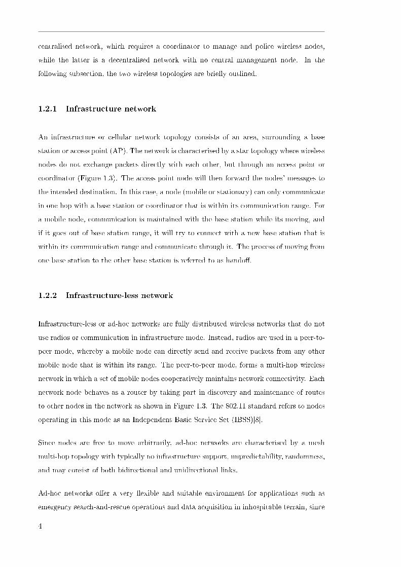
1.2.1 Infrastructure network
An infrastructure or cellular network topology consists of an area, surrounding a base
station or access point (AP). The network is characterised by a star topology where wireless
nodes do not exchange packets directly with each other, but through an access point or
coordinator (Figure 1.3). The access point node will then forward the nodes' messages to
the intended destination. In this case, a node (mobile or stationary) can only communicate
in one hop with a base station or coordinator that is within its communication range. For
a mobile node, communication is maintained with the base station while its moving, and
if it goes out of base station range, it will try to connect with a new base station that is
within its communication range and communicate through it. The process of moving from
one base station to the other base station is referred to as hando�.
1.2.2 Infrastructure-less network
Infrastructure-less or ad-hoc networks are fully distributed wireless networks that do not
use radios or communication in infrastructure mode. Instead, radios are used in a peer-to-
peer mode, whereby a mobile node can directly send and receive packets from any other
mobile node that is within its range. The peer-to-peer mode, forms a multi-hop wireless
network in which a set of mobile nodes cooperatively maintains network connectivity. Each
network node behaves as a router by taking part in discovery and maintenance of routes
to other nodes in the network as shown in Figure 1.3. The 802.11 standard refers to nodes
operating in this mode as an Independent Basic Service Set (IBSS)[8].
Since nodes are free to move arbitrarily, ad-hoc networks are characterised by a mesh
multi-hop topology with typically no infrastructure support, unpredictability, randomness,
and may consist of both bidirectional and unidirectional links.
Ad-hoc networks o�er a very �exible and suitable environment for applications such as
emergency search-and-rescue operations and data acquisition in inhospitable terrain, since
4

Figure 1.3: Basic network topologies
they allow the establishment of temporary communication without any pre-installed in-
frastructure. Although ad-hoc wireless networks o�er signi�cant bene�ts in terms of rapid
deployment and low cost, the traditional �at multi-hop routing approach su�ers from net-
work scaling.
1.2.2.1 Wireless mesh topology
Wireless ad-hoc network (peer-to-peer) architecture is sometimes referred to as wireless
mesh technology since a mesh network is a distributed network that generally allow trans-
mission only to a node's nearest neighbour. Nodes in this kind of network are generally
identical in terms of transmission capabilities and processing ability. Mesh networks are
probably a suitable model for large-scale wireless sensor networks that are distributed over
a given area. Since there are generally multiple paths between nodes, mesh networks tend
to be robust to failure of individual nodes or links. Another advantage of mesh networks
is that of a hybrid star and mesh topologies, where certain nodes can be designated as
coordinators or "group leaders" that can take additional functions such as the ability to
process and forward messages, and if a group leader is disabled, another node can take
over the leader's duties.
1.2.3 System architecture design challenges
WSNs have various unique requirements and constraints to make them practical and opera-
tional. Apart from the resources constraints, WSN may be subjected to harsh environment
5

conditions and dynamic network topology (wireless connectivity variation) that may even
cause part of WSN to disconnect due to link failures.
The choice of communication architecture will strongly in�uence WSN performance and
the e�cacy of routing and MAC protocols. For example, the network topology will in�u-
ence network performance parameters such as latency, energy consumption, capacity and
robustness. In addition, the complexity of MAC and data routing processes depends on
the network topology. Depending on the application under consideration (di�erent design
goals and constraints), the choice of network architecture can improve or degrade network
performance [5, 9, 10]. No standard and design rules have been followed in designing sen-
sor network architecture because of the broad range of applications, which have their own
purpose and requirements in terms of sensor hardware and network capability [11, 3, 12].
For example, apart from very few setups that utilise mobile sensors, most sensor network
architectures assume that sensor nodes are stationary. The dynamic nature of WSN will
impact the choice of routing, MAC level protocols and physical hardware.
Mobility in WSN will cause further topology variation compared to static con�gurations.
This will impose further complexity in protocol designs and may lead into further network
performance degradation. However, supporting mobility of sink nodes or cluster-heads
(gateways) is sometimes deemed necessary [13, 14, 15]. For example, [13], a case where
a mobile WSN was more energy e�cient than a static WSN, showed that in a static
WSN, nodes closer to the gateway sink always lose their energy �rst, thus causing the
overall network to expire. However, when the sink moves continuously, sensor node energy
dissipation is more e�cient. The sink movement can also decrease the number of hops
and therefore reduce the probability of error. While supporting mobility in some of WSN
applications can be advantageous, when connecting heterogeneous sensor network with
internet protocol (IP) based wire or wireless links, the traditional architecture (static) is
still more practical.
1.3 Communication Protocol Stack
Network devices, both wired and wireless, are commonly described by using the Open Sys-
tems Interconnection (OSI) seven-layer reference model [16]. This is the abstraction model
that was developed by the International Standards Organization (ISO), starting in the
1980s, to describe communication related protocols and services (Figure 1.4). The model
6
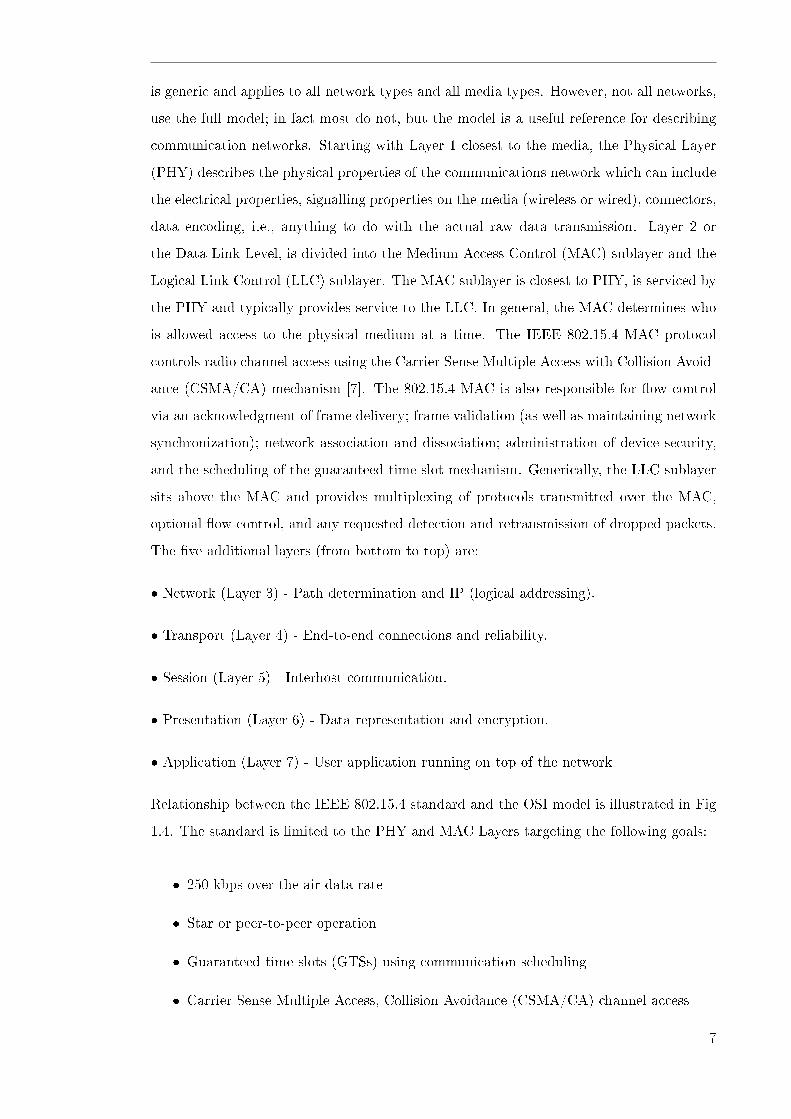
is generic and applies to all network types and all media types. However, not all networks,
use the full model; in fact most do not, but the model is a useful reference for describing
communication networks. Starting with Layer 1 closest to the media, the Physical Layer
(PHY) describes the physical properties of the communications network which can include
the electrical properties, signalling properties on the media (wireless or wired), connectors,
data encoding, i.e., anything to do with the actual raw data transmission. Layer 2 or
the Data Link Level, is divided into the Medium Access Control (MAC) sublayer and the
Logical Link Control (LLC) sublayer. The MAC sublayer is closest to PHY, is serviced by
the PHY and typically provides service to the LLC. In general, the MAC determines who
is allowed access to the physical medium at a time. The IEEE 802.15.4 MAC protocol
controls radio channel access using the Carrier Sense Multiple Access with Collision Avoid-
ance (CSMA/CA) mechanism [7]. The 802.15.4 MAC is also responsible for �ow control
via an acknowledgment of frame delivery; frame validation (as well as maintaining network
synchronization); network association and dissociation; administration of device security,
and the scheduling of the guaranteed time slot mechanism. Generically, the LLC sublayer
sits above the MAC and provides multiplexing of protocols transmitted over the MAC,
optional �ow control, and any requested detection and retransmission of dropped packets.
The �ve additional layers (from bottom to top) are:
� Network (Layer 3) - Path determination and IP (logical addressing).
� Transport (Layer 4) - End-to-end connections and reliability.
� Session (Layer 5) - Interhost communication.
� Presentation (Layer 6) - Data representation and encryption.
� Application (Layer 7) - User application running on top of the network
Relationship between the IEEE 802.15.4 standard and the OSI model is illustrated in Fig
1.4. The standard is limited to the PHY and MAC Layers targeting the following goals:
� 250 kbps over-the-air data rate
� Star or peer-to-peer operation
� Guaranteed time slots (GTSs) using communication scheduling
� Carrier Sense Multiple Access, Collision Avoidance (CSMA/CA) channel access
7

Figure 1.4: ISO reference model as adapted by 802.15.4 and ZigBee
� Acknowledged messaging for reliable data transfer
� Low power
� Short range operation
� Reasonable battery life
� Simple and �exible protocol
ZigBee network stack is built upon the IEEE 802.15.4 Standard and adds a communication
layer at layer 3 (network layer) and upper layers services through an application interface
(API). The standard provides all the advantages of a fully standardised communications
stack including full compatibility across applications and vendors [13]. In WSN, it is essen-
tial for all protocols in a communication stack to be optimised with respect to resources.
This thesis focuses on the two IEEE 802.15.4 standard layers for WSNs: PHY layer and
MAC.
1.4 Wireless Sensor Network Applications
The concept of WSNs is based on a simple �equation�:
8

Sensing + CPU + Radio + E�cient protocols = Many potential applications.
Developing an e�cient, e�ective WSN application, requires an understanding of both the
capabilities and limitations of the available hardware components and knowledge of modern
networking and distributed technologies.
WSN applications can be categorised based on the application area such as health, home,
environment and military applications; or by the way in which information is collected by
sensor nodes in a network, such as periodically sending information to the data sink, event
triggered and polling applications.
Currently, wireless sensor networking can o�er a wide range of potential monitoring and
control applications including [17, 18, 19];
� pollutant monitoring
� habitat monitoring
� environmental monitoring,
� areas such as security surveillance,
� rescue missions in inhospitable terrain,
� tra�c surveillance,
� health care (patient care),
� robotic exploration,
� industrial and manufacturing automation,
� building and structure monitoring,
� inventory tracking,
� home appliances, and
� farming.
In industries, sensor networks may include sensing and detecting or diagnosing di�erent
parameters of interest, and industrial or appliance automation. Moreover, sensor networks
9

can be used in infrastructure projects such as power grids, water distribution, waste dis-
posal, security and even battle�elds.
Sensor networks have been used for vehicular tra�c monitoring and control. However, these
networks and the communication network that connect them are costly, thus tra�c control
is usually limited to few critical points. Inexpensive reliable ad-hoc wireless networks will
completely change the landscape of tra�c control and monitoring.
Another more radical concept is having sensors attached to each vehicle and as vehicle
pass each other, they can exchange information on the location of tra�c jams and speed
and density of tra�c, the information might be generated by ground sensors.
Electric-power-system monitoring and diagnostic systems are typically realised through
wired communications. However, such systems require expensive communication cables
to be installed and regularly maintained, and thus, they are not widely implemented to-
day because of their high cost. A more cost e�ective wireless monitoring and diagnostic
system (WSN) will bring signi�cant advantages over traditional communication technolo-
gies, including rapid deployment, low cost, �exibility and aggregate intelligence via parallel
processing.
In the near future, sensor networks will be able to support new opportunities or applica-
tions for interaction between humans and their physical world and speci�cally WSNs are
expected to contribute signi�cantly to pervasive computing and space exploration. De-
ploying sensor nodes in an attended environment will provide tremendous possibilities for
the exploration of new applications in the real world.
In many applications, such as forest �re monitoring or intruder detection, user intervention
and battery replenishment is not possible. Since the battery lifetime is directly related to
the amount of processing and communication involved in these nodes, optimal resources
utilisation becomes a major issue.
1.5 Application Requirements and Design Goals
Most studies of wireless networks tackle some of the problems associated with them. Cur-
rently, a wide-range of research in wireless networks thrives on ways to improve the quality
of service (QoS) of wireless networks for multimedia applications. WSN applications will
10

usually have di�erent quality-of-service (QoS) requirements and speci�cations such as re-
liability, latency, network throughput, and power e�ciency. The primary performance
objectives of wireless sensor networks in most cases are energy conservation, throughput
improvement, scalability and self-con�guration, whereas fairness and temporal delay are
often secondary issues [20].
Since sensor nodes share a common wireless medium, an e�cient medium access control
(MAC) operation is required; however other issues which cannot be ignored include topol-
ogy changes or mobility, multi-hop communication, self-con�guration, unattended nature
of wireless sensors (power), connectivity, and throughput improvement. In particular, a
WSN application will require a high level of system integration, performance, and produc-
tivity.
To design good protocols for wireless sensor networks it is important to understand the
parameters that are important to the sensor applications and in this thesis the following
metrics are used.
1.5.1 System lifetime
A sensor network is expected to have a long operational life to further reduce the cost of
maintenance and deployment. In WSNs, energy e�ciency is often a critical issue due to a
limited battery life [3]. Typical wireless sensor nodes are inherently resource constrained as
are usually powered by batteries or harvested energy, and network lifetime usually depends
on the reliance of sensor nodes. Power source replenishment is not possible in most of the
application scenarios. Energy consumption in a WSN can be minimised by: e�cient data
aggregation, e�cient routing, e�cient MAC layer with power management, and topology
management using transmission power control. The system's lifetime can also be extended
through energy-e�cient techniques at all system hierarchy or protocol stack levels.
Since sensor node main tasks include sensing or collecting events, processing data, and data
transmission, power consumption can be categorised amoung these operations. Moreover,
as sensor nodes become more compact, the challenges increase for processing, communica-
tion and storage capabilities.
11

1.5.2 Self-organisation and self-con�guration
A wireless sensor network should self-organize and maintain connectivity e�ciently and
speci�cally the MAC protocol manages self con�guration, i.e., ability to start a new PAN,
associate or disassociate with an exiting network, and synchronize if required.
It is important that sensor networks can be easily deployed possibly in remote or dangerous
environments where nodes have to communicate even without established network infras-
tructure. To function in such ad-hoc settings, sensor networks should be self-con�guring
(no global control to setup or maintain the network); thus such ad-hoc networks must be
able to achieve neighbour discovery, topology organisation and topology reorganisation.
During the neighbour discovery phase, every node in the network gathers information
about its neighbors and maintains that information in appropriate data structures. This
information is obtained periodically either by sending short packets named beacons, or
by promiscuously snooping on the channel to detect the activities of neighbours. The
communication among sensor nodes depend on topology organisation (section 1.2), and
reorganisation in case of changes in a network, such as communication loss.
1.5.3 Reliability
Reliability or fault tolerance of a sensor node is the ability to maintain the sensor network
functions without any interruption due to sensor node failure, for example, through lack
of energy, physical damage or communication problems. Therefore the node power source,
communication links and overlying protocols will contribute to system reliability.
1.5.4 Scalability
The vision of a mesh networking is based on the strength in numbers because unlike cell
phone systems, service is not denied when too many devices are active in a small area. In
a WSN, several sensors may be deployed to study a phenomenon of interest to users. The
issue is: how well does the network perform, with an increasing number of nodes and node
density, for coverage area, energy consumption, reliability and accuracy?
12

1.5.5 Latency
The time delay of sensor node information (latency) is another important performance
variable because long delays due to processing or communication may be unacceptable
depending on an application.
1.5.6 Packet Error Rate (PER)
Packet Error Rate (PER), is the percentage delivery ratio, which is de�ned as the number
of data packets correctly received by the destination node over the total number of packets
generated by source nodes. This re�ects the degree of reliability achieved by the network
for successful transmissions.
1.5.7 Throughput
The channel e�ciency or throughput is de�ned as the fraction of time that the channel is
used to successfully transmit payload bits or the fraction of data tra�c correctly received
by the node over a speci�ed period.
1.5.8 Productivity
Another important factor for WSNs is the system productivity; this has two aspects, the
most important being how well it assists the end user to do their task, i.e. to meet col-
laborators expectations. However, productivity is also about reducing the costs involved
in a sensor network over its lifetime including planning, node hardware, deployment, trou-
bleshooting and maintenance.
For any emerging technology, economic drivers and cost bene�ts are pivotal issues which
could dramatic a�ect market growth and sensor networks face several relevant challenges.
The �eld arguably emerged due to the commercialisation of cheap, low-power, single-chip
microcontrollers and radios. These components emerged due to rapid growth of global
electronics industries such as cell phones and wireless remotes. The biggest challenge in
WSNs is developing e�ective communication systems that will run unattended for years in
an increasingly energy e�cient manner.
13

1.6 Research Motivation and Challenges
The emerging �eld of WSN research combines numerous disciplines and addresses a com-
bination of the major challenges in sensor techniques, embedded techniques, distributed
information processing, mobile computing and wireless communication [21, 22]. These net-
works di�er from conventional wireless networks due to their hardware limitations of low
cost and severe energy constraints for computation and communication, low data rates,
potentially huge network size and a wide range of information �ows [20, 22]. WSNs will
have to cope with limited resources placed on individual devices, i.e. transceivers, em-
bedded microprocessors will limited processing and memory capability, must implement
and process complex networking protocols. A sensor node's, envisioned to shrink to cubic
millimeter scale, poses stringent limitations on its processing, communication and stor-
age capabilities. Despite continued advances in micro-electromechanical systems (MEMs),
lower-power very large-scale integration (VLSI), and computing, aligning desired capabil-
ities with compactness remains challenging [23].
Sensor networks, similar to Mobile Ad-hoc networks (MANET), are envisioned to have
dynamic, sometimes rapid-changing, randomly distributed, multi-hop topologies that are
composed of relatively limited wireless link bandwidth. WSN can be deployed with a large
number of unattended nodes and therefore the underlying network architecture has also
become one of the challenging areas in wireless sensor networks research [17, 24].
It is well established that the wireless medium is characterised with high bit error rates
(BER) compared to wired mediums [25]. Errors in wireless mediums occur in bursts while
in traditional wired networks errors occur randomly. Furthermore, it cannot be assumed
that a fully connected topology exists between nodes in wireless networks, but rather a
logical network topology that is constantly adapting to node or user movement. Therefore,
wireless ad-hoc networks are characterised by unreliable links, burst errors and dynamically
changing network topologies.
Running e�ective WSN communication systems, unattended for years from a limited en-
ergy resource, requires both energy-e�cient, robust hardware and an e�cient software
management system. Emerging WSNs are likely to be more energy-e�cient with reliable
connectivity, despite the greater constraints on battery capacities and connectivity im-
posed by the compactness and increasing density of new wireless devices. To minimize the
14
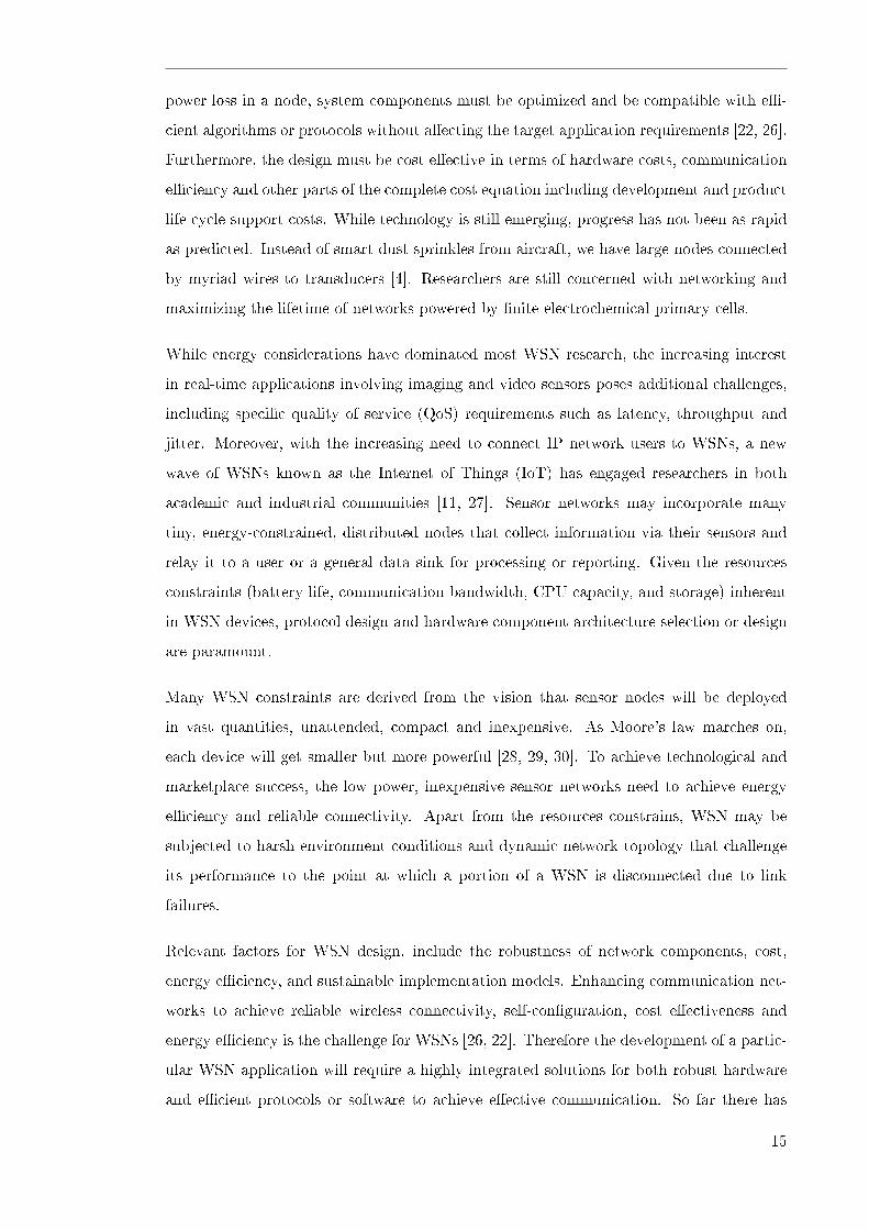
power loss in a node, system components must be optimized and be compatible with e�-
cient algorithms or protocols without a�ecting the target application requirements [22, 26].
Furthermore, the design must be cost e�ective in terms of hardware costs, communication
e�ciency and other parts of the complete cost equation including development and product
life cycle support costs. While technology is still emerging, progress has not been as rapid
as predicted. Instead of smart dust sprinkles from aircraft, we have large nodes connected
by myriad wires to transducers [4]. Researchers are still concerned with networking and
maximizing the lifetime of networks powered by �nite electrochemical primary cells.
While energy considerations have dominated most WSN research, the increasing interest
in real-time applications involving imaging and video sensors poses additional challenges,
including speci�c quality of service (QoS) requirements such as latency, throughput and
jitter. Moreover, with the increasing need to connect IP network users to WSNs, a new
wave of WSNs known as the Internet of Things (IoT) has engaged researchers in both
academic and industrial communities [11, 27]. Sensor networks may incorporate many
tiny, energy-constrained, distributed nodes that collect information via their sensors and
relay it to a user or a general data sink for processing or reporting. Given the resources
constraints (battery life, communication bandwidth, CPU capacity, and storage) inherent
in WSN devices, protocol design and hardware component architecture selection or design
are paramount.
Many WSN constraints are derived from the vision that sensor nodes will be deployed
in vast quantities, unattended, compact and inexpensive. As Moore's law marches on,
each device will get smaller but more powerful [28, 29, 30]. To achieve technological and
marketplace success, the low power, inexpensive sensor networks need to achieve energy
e�ciency and reliable connectivity. Apart from the resources constrains, WSN may be
subjected to harsh environment conditions and dynamic network topology that challenge
its performance to the point at which a portion of a WSN is disconnected due to link
failures.
Relevant factors for WSN design, include the robustness of network components, cost,
energy e�ciency, and sustainable implementation models. Enhancing communication net-
works to achieve reliable wireless connectivity, self-con�guration, cost e�ectiveness and
energy e�ciency is the challenge for WSNs [26, 22]. Therefore the development of a partic-
ular WSN application will require a highly integrated solutions for both robust hardware
and e�cient protocols or software to achieve e�ective communication. So far there has
15
been no clear guidelines or design rules that have been followed in designing sensor net-
work architectures because of the wide range of sensor applications, with each application
having its own unique purpose and performance requirements i.e, various hardware and
network capabilities.
1.6.1 Application requirements and resources constraints
In general, the design and implementation of WSNs are constrained by four types of re-
sources: energy, memory, communication and processing. The increasing interest in real-
time applications along with introduction of imaging and video sensors has fostered ap-
plications that require certain end-to-end performance guarantees, this posing additional
challenges in both QoS aware network protocols and energy e�ciency. For example, many
military and civil applications, such as disaster management, combat �eld surveillance,
and security, will be required to detect moving targets.
It is essential to di�erentiate between an application's QoS objectives and constraints.
Communication subjected to QoS requirements can be exceptionally challenging in a
resource-constrained environment such as in sensor networks [5, 23]. The diversity of WSN
applications will lead to di�erent speci�cations and quality-of-service (QoS) requirements,
including reliability, latency, network throughput, and power e�ciency.
1.6.2 Integrating WSN with internet and Alternative Technologies
The adoption of WSNs will increase as they become more integrated with existing technolo-
gies such as internet, mobile and satellite communication. Currently, there are two main
architectures for connecting WSN to the internet, a proxy based approach and internet
protocol (IP) integration at the sensor node level (also referred to as IP stack).
The connection of a WSN to the internet through the former is achieved by using a proxy
node that acts as a gateway to the internet for sensor nodes that communicate through
separate WSN protocols. In this case, WSN and IP have di�erent routing protocols , and
therefore the proxy node acts as a protocol mapping device, converting IP to or from,
to connect the WSN to the internet. The proxy node acts as a default sink for sensor
nodes and stores the sensor readings. When a remote system requests information from
sensor data, cached results (in a local database) are returned by the proxy node. Likewise,
16

when requesting real-time information, a separate request will be sent from the proxy node
to the sensor node and therefore regardless of the data retrieval method used, no direct
connection between the querying system and the sensor node is established. Usually, the
proxy is achieved at the application layer or may be applied at the network layer, where a
sink or proxy node queries the network without the use of a local database. This approach
allows an existing WSN to be connected to the internet with minimum changes. Currently,
an application level proxy server is often used to separate the sensor network from the rest
of the enterprise network. The application level proxy o�er rich translation, caching, and
support for reliable networking.
The IP based approach is achieved by using IP stack as the routing protocol inside the
WSN itself and therefore there is no need to use proxy node. The use of IP on WSN
provides signi�cant advantages by providing more ubiquitous services. However such ad-
vantages come with a price including increased frame header overhead, addressing scheme,
limited bandwidth, protocol complexity, memory and limited energy. For example, the
maximum size allowed for 802.15.4 frame is 127 bytes, MAC header ranges 9-39 bytes,
and an additional 20 (IPv4) to 40 (IPv6) bytes will be consumed by the IP header. To
overcome this unacceptable overhead and allow IPv6 packet transportation over 802.15.4
frames, techniques such as those found in the 6LoWPAN standard must be used. Using
a complete protocol stack, such as Zigbee protocol stack, which uses a proprietary layer 3
protocol on top of the IEEE 802.15.4 standard using IPv4 or IPv6 standards, would largely
simplify the integration of these devices into a globally connected Internet of Things (IoT).
Another area of WSN integration is a suitable satellite remote sensing using system such
as SPOT-5, 3G, 4G, 802.11 and 802.16. It is likely that a combination of current and
future technologies will be used for future WSN deployment. Furthermore, the growing
focus on using cognitive radios opens up new opportunities for current sensor networks to
merge with other wireless services in order for systems to overcome some of the current
limitations and to broaden WSN application areas.
1.7 Research Questions and Contributions
The main object of this thesis is to enhance the performance of WSN to maintain reliable
network connectivity, improve scalability and save energy. The study focuses on the IEEE
802.15.4 MAC/PHY layers and the carrier sense multiple access with collision avoidance
17

(CSMA/CA) based networks. So the main research question is �how and what can be done
to improve the performance of WSNs to maintain reliable network connectivity, scalability
and energy e�ciency in the IEEE 802.15.4 based networks?� To answer this question, this
research consists of four semi-independent areas of study to which the following research
questions are addressed:
1. How can we speci�cally test multi-hop TPC communication versus single-hop com-
munication using typical wireless sensor node hardware parameters?
2. What is the performance advantage of using multi-hop TPC in energy constraint
WSNs instead of a single-hop in terms of energy e�ciency and other important
performance parameters?
3. What is the impact of beacon interval (BI) and number of nodes during WSN associa-
tion and synchronization stages in terms of energy and association or synchronization
time?
4. How can we improve the performance of WSNs during association and synchroniza-
tion stage (self-con�guration)?
5. What is the impact of the number of times the clear channel assessment (CCA) is
performed in the 802.15.4 MAC during frame transmission in terms of throughput,
packet error rate, delay and energy consumption for both hidden and non-hidden
nodes in a network ?
6. What can be done to improve the performance of the 802.15.4 MAC during frame
transmission stage?
7. How can Markov chains be used to accurately model the IEEE 802.15.4 slotted
CSMA/CA ?
8. What is the relationship between di�erent performance variables and the MAC pa-
rameters derived from the Markov Chains?
The main research contributions of this thesis are:
� In chapter 4, a new detailed approach is presented for testing transmission power
control (TPC) for multi-hop and single-hop WSNs at the physical layer using real
18

hardware parameters. Following this approach, energy consumption performance
results via simulation and a numerical model are presented. Both the radiation
and electronic components of the energy consumption are characterized, and results
indicate that sending packets using a short-range multi-hop path, instead of a single-
hop, does not necessarily save energy as suggested by some researchers [31, 32, 33].
Moreover, transmitting in single-hop networks at lower transmission power levels,
while still maintaining reliable connectivity, reduced energy consumption by up to
23%. Furthermore, the research shows that both packet collisions and delays a�ect
the performance of WSNs that have an increased number of hops. Since the use
of TPC in star topology or cellular networks transmission can save energy, we rec-
ommend cluster based (hybrid) or similar topology over completely multi-hop topol-
ogy. The relationships among protocol layers are also revealed, possible improvement
suggested, insights are provided into challenges associated with developing wireless
sensor networks protocols and the signi�cance of TPC is highlighted;
� In chapter 5, performance of the 802.15.4 MAC is evaluated during device association
and synchronization with the PAN coordinator; this shows the impact of beacon
interval and the number of associating nodes in terms of association time delay
and energy consumption in stationary wireless sensor networks. Results illustrate
that energy consumption and association time increase with increasing number of
nodes associating with a coordinator. Moreover, short beacon intervals consume more
energy due to the frequency of beacon frames that nodes have to keep track of to
maintain synchronization. However, short beacon intervals reduce the time required
for the nodes to associate, in contrast to longer beacon intervals that are undesirable
for real time and mobile applications. Furthermore, for longer beacon intervals, BO=
12 to BO=14, there is an abrupt increase in energy consumption as the number of
associating nodes increases, even for only four nodes. This appears to be the �rst
investigation of the performance of the 802.15.4 MAC beacon interval setting and
the number of associating nodes. To conserve energy in WSNs, we expect to use
longer beacon interval (BI) and shorter active periods (SD) so that the nodes can go
into inactive or sleep state during CAP to save energy. To date the longest beacon
interval is 251.66s (about 4 minutes). Our results demonstrate that even with 7 nodes
connected to the PAN coordinator, the association delay and energy consumption
due to synchronization, increase. The question is whether the association energy
consumption will outweigh the bene�t of duty cycle power management for larger
19
beacon intervals, as the number of associating nodes increases?
� In chapter 6, the impact of the number of times the CCA is performed in the 802.15.4
MAC during frame transmission is studied in terms of throughput, packet error rate,
delay and energy consumption is presented. Both hidden and non-hidden nodes in
a network system are considered. Results indicate a serious network performance
degradation even with only a small number of hidden nodes in a network. Following
these results a propose cross layer (PHY-MAC) mechanism to save energy, reduce
interference, improve scalability and reliability, and reduce packet collisions due to
hidden terminals is presented.
� Chapter 7 contains a proposed model to capture essential features of the IEEE
802.15.4 slotted CSMA/CA by using the Discrete Markov chain. The relationships
for the successful transmission probability, throughput and average energy consump-
tion are derived.
1.8 Thesis Structure
The remainder of the thesis is organised as follows. Chapter 2 provides the literature re-
view on WSNs, including review on medium access control (MAC) and the IEEE 802.15.4
standard. The research questions and methodological framework layout for this research
is presented in Chapter 3. Chapter 4 provides TPC investigation in multi-hop and single-
hop WSNs, and a detailed description of a new approach to testing TPC in multi-hop
networks at the physical layer. In Chapter 5, performance analysis of the 802.15.4 MAC
during device association and synchronization with the PAN coordinator is presented. In
Chapter 6, performance analysis of Slotted IEEE 802.15.4 MAC Clear Channel Assess-
ment for both hidden and non-hidden nodes, and a proposed algorithm for improvement
are presented. The developed Markov Chain analytical model is presented in Chapter 7.
Finally, conclusions and a discussion on future work are given in Chapter 8.
20

Chapter 2
Literature Review
The aim of this chapter is to provide, through selective references to some of the
literature, an overview of previous work on topics that provide the necessary
background to this research. The literature review focuses on a range of WSN
research, the IEEE 802.15.4 standard and key concepts, and theories relating
to this research.
2.1 Introduction
Research on Sensor Networks and Mobile Ad-hoc Networks (MANET) is receiving in-
creased interest within the research community [34, 24, 35, 5]. MANETs have been con-
sidered for a wide range of new applications since the early research e�orts of the Defense
Advanced Research Projects Agency (DARPA) research program on packet radio networks
for military use [36]. Among these new applications include that of wireless sensor network
(WSN). Research in wireless sensor networks have strong links to wireless ad-hoc networks.
Both WSN and MANET relate to distributed communication between nodes in an infras-
tructureless environment. Currently, the research focus on Ad-hoc radio techniques have
migrated to dual-use and commercial use in areas such as home computing, public wire-
less LAN and wireless sensor networks. Wireless sensor networking o�er a wide range
of potential applications including security surveillance, tra�c surveillance, environment
monitoring, medical systems, robotic exploration, data acquisition in industries, farming
and rescue missions in inhospitable terrain [18, 17, 37, 38, 39]. There are numerous factors
as to why ad-hoc wireless sensor networks are receiving increased attention in research
communities. Among these factors are the signi�cant bene�ts of rapid deployment, the
21

wide range of potential applications, low setup and maintenance costs, the use of license-
free spectrum, along with the continual decrease in size and cost of sensors. These factors
have fostered intensive research addressing the potential of associating several sensors to
gather and process information via wireless connectivity. Networking unattended sensor
nodes is expected to have a high impact on the e�ciency of military and civil applications
soon[17, 40]. For technological and marketplace success, the low power, inexpensive sen-
sor networks need to achieve or attain energy e�ciency and reliable connectivity. Apart
from the resource constraints, WSN may be subjected to harsh environment conditions
and dynamic network topology that challenge its performance to the point at which a
portion of a WSN is disconnected due to link failures. The IEEE 802.11 standards lack the
ability to provide all these features (resilience); however these standards provide the base
for research communities to work on building or creating new standards able to deal with
di�erent applications [8]. Furthermore, given the broad use of the IEEE 802.11x standard,
it is expected to have existing nodes using the IEEE 802.11 standard in a real applica-
tion scenario. Currently an increased number of researchers are working with or on a new
IEEE 802.15.4 standard technology, commonly known as ZigBee technology. ZigBee was
adopted in 2003, and is based on or derived from the 802.15.4 low-rate, Wireless Personal
Area Network (WPAN) standard [41, 42]. Bluetooth (IEEE 802.15.1) is another prominent
wireless technology in the area of wireless sensor networks.
2.2 An Overview of Wireless Sensor Networks
Sensor networks are distributed networks made up of small sensing devices equipped with
a processor, memory and capability for short range wireless communication. The di�erence
from conventional networks is that they have severe energy constraints, low-rate data, and
a wide range of information �ows [20, 43, 44]. Normally sensor network consists of large
number of distributed nodes that organise themselves into a multi-hop wireless network.
Ad-hoc networks self-con�guring, infrastructureless and multi-hop mechanism can improve
the throughput and power e�ciency of the network. The implementation of sensor networks
in this research can consequently be tailored to speci�c applications and can be formed
from whatever network nodes available.
Sensor networks, similar to Mobile Ad-hoc networks (MANET), are envisioned to have
dynamic, sometimes rapid-changing, randomly distributed, multi-hop topologies that are
22
composed of relatively limited wireless link bandwidth. WSN can be deployed with a large
number of unattended nodes and therefore the underlying network architecture has also
become one of the challenging areas in wireless sensor networks research [17, 24]. Whilst ad-
hoc networks have been the subject of a signi�cant amount of research and development,
currently, the emerging �eld of Wireless Sensor Networks research combines numerous
disciplines and poses a combination of challenges facing modern computer science, wireless
communication and mobile computing [45, 3, 5, 46]. WSNs can be deployed in large
numbers of unattended nodes and therefore the underlying network architecture has also
become one of the challenging areas in wireless sensor networks research [17, 24].
It is well established that the wireless medium is characterised with high bit error rates
(BER) compared to wired mediums [25]. Errors in wireless mediums occur in bursts while
in traditional wired networks errors occur randomly. Furthermore, we cannot assume a
fully connected topology between nodes in wireless networks, but rather a logical network
topology that is constantly changing depending on node or user movement from one point
to another. Therefore, wireless ad-hoc networks are characterised by unreliable links, burst
errors and dynamically changing network topologies.
Most of the studies on wireless networks are based on tackling some of the problems as-
sociated with wireless networks. Currently, a wide-range of research in wireless networks
thrives on ways to improve the quality of service (QoS) of wireless networks for multime-
dia applications [47, 12]. With wireless sensor networks, one needs to look at all these
ongoing research issues along with other issues that are unique to wireless sensor networks
(WSN) and ad-hoc networks. The primary performance objectives of wireless sensor net-
works in most cases are energy conservation, throughput improvement, scalability, and
self-con�guration, whereas fairness and temporal delay are often secondary issues [20, 18].
Since sensor nodes share a common wireless medium, an e�cient medium access control
(MAC) operation is required without isolating other issues such as topology changes or mo-
bility, multi-hop communication, self-con�guration, unattended nature of wireless sensors
(power), connectivity, and throughput improvement.
2.3 Sensor Node Hardware Platform
A low-rate wireless personal area network (LR-WPAN) platform (also referred to sensor
node or device) is typically designed with a separate microcontroller (processor), radio
23

transceiver, power supply (battery), sensor, storage and a number of peripherals (Figure
2.1). Currently, most of the sensor nodes commercially available are made up of o�-
the-shelf components also known as COTS (commodity of the shelf) mounted on a small
printed circuit board [48, 49]. However, more single chip solutions with integrated protocol
hardware implementation are also becoming more available.
Figure 2.1: Sensor node hardware
2.3.1 Processing module (Micro-controllers & processors)
The processing module is the core of the platform, around which are arranged all sensor
node functions and procedures needed to perform a particular sensing task. In the PC
era the emphasis was on faster processors; unfortunately, this increased power consump-
tion unacceptable for modern wireless sensor systems. In the current era of connected
intelligence, embedded process performance and processing power consumption need to be
balanced along with integrated transceiver and sensors. Depending on WSN application
requirements such as processing speed, energy e�ciency and costs, there are several low-
end and high-end processors or microcontrollers that could be selected from the literature
[50, 51, 52]. A lower end microcontrollers (MCU) have a simple internal processor with bus
width of between 4 and 16 bits, with only on-chip memory, and no interfaces to external
RAM. In contrast, microprocessors used in personal computers or other general purpose
applications. High end devices contain complex processors with bus width typically 32
or even 64 bit system bus, higher clock rates devices, caches and interfaces to external
memories. Moreover, the complex processing module may be capable of energy aware pro-
24

cessing and pre-processing of received data as well as featuring multiple CPUs for faster
processing.
There is a confusing array of processors or microcontrollers that can be chosen for a partic-
ular WSN application, the �eld to choose from is quite large and can be a confusing task.
However, the following guide can assist with choosing the right processing module for an
electronics development project. The �rst task will be to determine the application sys-
tems critical priorities, such as processing power, power consumption, operating voltage,
operating temperature, �exibility, and cost. The next task is to develop or determine a
more suitable solution from available technologies (hardware or protocols) that can support
such a project. The choice of a processor should be driven by the desired tradeo� between
processing capabilities, energy consumption (for di�erent mode), price and �exibility.
Table 2.1 provides details on the characteristics and capabilities of some of the most popular
processing modules employed in various state-of-the-art sensor nodes. Low power, low-cost
and simple instruction sets are used such as 8-bit Atmel's ATmega128L CPU on the Mica
motes, and the 16-bit Texas Instrument's (TI) MSP430 family on the Telosb motes. The
MSP430 from TI has some of the best power saving, and power consumption �gures in the
industry with a good supply operating voltage range.
The main factors a�ecting a controller's hardware power consumption include the supply
operating voltage, clock frequency at which the controller operates, peripherals enabled,
external switching activity, and external components required in the system (particularly
power ampli�ers). This can be related using the following expression:
PdynamicαCV2ddfclk, (2.1)
where C is the collective switching capacitance, Vdd is the supply voltage, and fclk is the
clock frequency. Lowering the supply voltage Vdd can signi�cantly reduce the amount of
energy consumed because of the quadratic relationship between power and Vdd as shown
in the equation 2.1.
Processors and transceivers have several power down modes or power saving features (Ta-
bles 2.1 and 2.2) that can be used to conserve energy. The low power modes such as
25

Table 2.1: Processor features and comparison
Micro-
controller/
Micropro-
cessor
CPU Clock speed
(max
operating
frequency)
Memory
(onchip & Ex-
ternal/�ash
memory)
Power saving features Platform
using
Operat-
ing
volt-
age
Operat-
ing
Temp.
Average
Price
MSP430-
F5xx (TI)
[53]
16-bit
AVR
microcon-
troller
20MHz 16/18 KB
onchip RAM &
128/256KB KB
external.
Interface
5 low power modes
(LPM0-LPM4). Normal
state power consumption
1.8mA/3mA. Low state
current consumption <
1µA
TelosB,
EyesIFX,
Scatterweb,
WISAN,
Kmote
1.8 to
3.6V
-40°C
to
+85°C
$3.92
ATmega128
(Atmel) [52]
8-bit AVR
micropro-
cessor
16MHz and
8MHz
4 KB onchip
RAM & 128
KB external
Sleep 20µA ; Active 8mA MicaZ,
Btnode,
Waspmote,
EmberNet,
Iris Mica2
4.5 to
5.5V
and 2.7
to 5.5V
-55°C
to
+125°C
$14.90
and
$12.90
ATmega64/L
(Atmel) [52]
8-bit AVR
(at-
mega64L)
16 MHz and
8 MHz;
64 KB Repro-
grammable
Flash program
memory; 2 KB
EEPROM; 4
KB Internal
SRAM
Six Sleep Modes: Idle,
ADC Noise Reduction,
Power-save, Power-down,
Standby and Extended
Standby.
4.5 to5.5Vand
2.7-
5.5V
-40°C
to
+85°C
$8.90
HCS08
(Freescale)
[51]
8-bit
microcon-
troller
using
M68HC08
8 MHz at 5V
oper. voltage.
4 MHz at 3V
oper. voltage
256 bytes ofon-chip RAM.
8,192 bytes
user program
FLASH
memory
20 nA power-down mode.
Can reduce power to 0.7
microamp (uA) - Up to 40
MHz CPU/20 MHz bus at
2.1 V and 16 MHz CPU/8
MHz bus at 1.8 V
1.8 to
3.6V
- 40 to
+125
$6.50
PXA270
(INTEL)
PXA
Xscale
Processor
32-bit
ARMv5
architec-
ture
processor.
312 MHz, 416
MHz, 520
MHz and 624
MHz.
32 KB
instruction
cache; 32 KB
data cache; 2
KB �mini� data
cache; 256 KB
of internal
SRAM
Dynamically drops the
core's voltage and clock
frequency according to
demand (4 low-power
modes). Supply voltage
may be reduced to 0.85 V.
HP iPAQ
hx2495
Pocket PC
2.25 to
3.7V ;
5V
-40°C
to
+85°C
$32.97
PXA271-
PXA272
(INTEL)
[54]
PXA
Xscale
Processor
32-bit
ARMv5
13, 104, 208
MHz or 416
MHz for 271
and 312 MHz,
416 MHz or
520 MHz for
272
32 MB �ash &
32 MB of
SDRAM; 32
KB data cache;
32 KB
instruction
cache; 256 KB
of internal
SRAM
Dynamic voltage andfrequency management (4low-power modes).
Supply voltage may be
reduced to 0.85 V.
imote2
(A271), Intel
Stargate 2
(A271),
Pocket PCs,
PDAs, GPS
Navigation
systems
2.25 to
3.7V;
5V
-40°C
to
+85°C
$50.14
26
sleeping mode can dramatically increase the battery life span depending on the applica-
tion. For example, in a periodic sampling application where sensor nodes are most likely to
spend 99.9% of their time in sleep mode, the consumption is close to zero [55]. Obviously
if the MCU is allowed to run in its normal state at all times, then the coin cell battery
will last for less than seven hours, but if it is intelligently switched to its lower power state
most of the time, the battery can last more than two years. Thus implementing the power
management scheme and using the right hardware can dramatically increase battery life.
For a platform, with a separate microcontroller and a radio transceiver, communication
between the microcontroller and the transceiver is via a serial bus such as SPI (Serial
Peripheral Interface) or UART (Universal Asynchronous Receiver or Transmitter). The
SPI has a full-duplex capability supporting data rates of up to 20 Mbps compared to a
common two wire interface, I2C bus that supports 100 or 400 Kbps data rates. This allows
simple, e�cient communication among devices controlled by one master (microcontroller).
2.3.2 Transceivers
A wireless communication module (transceiver) is responsible for data transmission and
reception via a speci�c radio channel and modulation or demodulation and spreading or
de-spreading techniques. An IEEE 802.15.4 network may operate in one of the three
Industrial, Scienti�c, Medical (ISM) frequency bands: 2.4 GHz, 915 MHz and 868 MHz as
illustrated in �gure 2.4 in section 2.10.
In this thesis, we focus on transceivers operating in the 2.4 GHz band of the IEEE 802.15.4
standard. Selecting a speci�c receiver-transmitter architecture for a particular application's
performance requirements, requires careful examination of the transceiver's key features
such as data rates, the number of channels that can be used, channel bandwidth, energy
consumption, modulation type, receiver sensitivity, transmit power levels, link budget,
ease-of-integration, and requirement of external components that have signi�cant function
and cost implications. In some cases there is a clear tradeo� between a high performance
chip-set providing high data rates against a basic communication chip-set with a lightweight
protocol and low power cost. For example, the 802.11b transceiver card has higher trans-
mission ability at 11Mbit/s but also consumes more power, while the 802.15.4 on CC2420
chip-set has lower power consumption but with a lower transmission rate, 250kbit/s and
communication range [56, 50].
27

Table 2.2 provides details on the characteristics and capabilities of some of the available
transceivers in the literature as a guide into selecting a desirable transceiver for a particu-
lar WSN development project. For a example from the table (Table 2.2) we observe that
the radio may consists di�erent operation modes (e.g., transmit, receive, idle, and sleep)
for power management purposes [22]. In terms of energy consumption, sleep mode power
consumption, radio operating voltage will in�uence the power management algorithms.
Also most of the transceivers available operate at Temperature ranging -40 oC to 80, apart
from the CC2520 [53] which can operate up to 125 oC, this can be useful when considering
application such as �re detection. Other important transceiver features include extensive
hardware support for MAC support such as data encryption, data authentication, clear
channel assessment, link quality indication and frame timing information; transceiver re-
ceiver sensitivity and transmission power will a�ect the transmission range apart from
antenna gains and heights as the link budget is determined by adding together their abso-
lute values [22].
2.3.3 Integrated Chips
There are several commercially-available integrated chips , for example the CC2431, which
combines the CC2420 RF transceiver with an industry-standard enhanced 8051 micro-
controller [53]. The CC2431 is a true System-On-Chip (SoC) for wireless sensor net-
working with the most competitive industry leading ZigBee® protocol stack (Z-Stack�)
from Texas Instruments. One major drawback of the CC2430 is its limited debugging
capability. It o�ers a very limited low level access through the two-wire debug interface.
The ATmega128RFA1 is derived from the ATmega1281 microprocessor combined with the
AT86RF231 radio transceiver [52]. Other SoC include the Freescale Semiconductor, its
manufacturer provides a variety of 802.15.4 SoCs [51]. The MC1322x series is highly in-
tegrated solution with a 802.15.4 compliant on-chip transceiver and an ARM7 processor.
With time we expect more integrated chips in the market for WSN platforms.
2.3.4 Power source
The power source module supplies power to a sensor node, which determines a sensor node's
lifetime. The electrode material and the di�usion rate of the electrolyte's active material
28
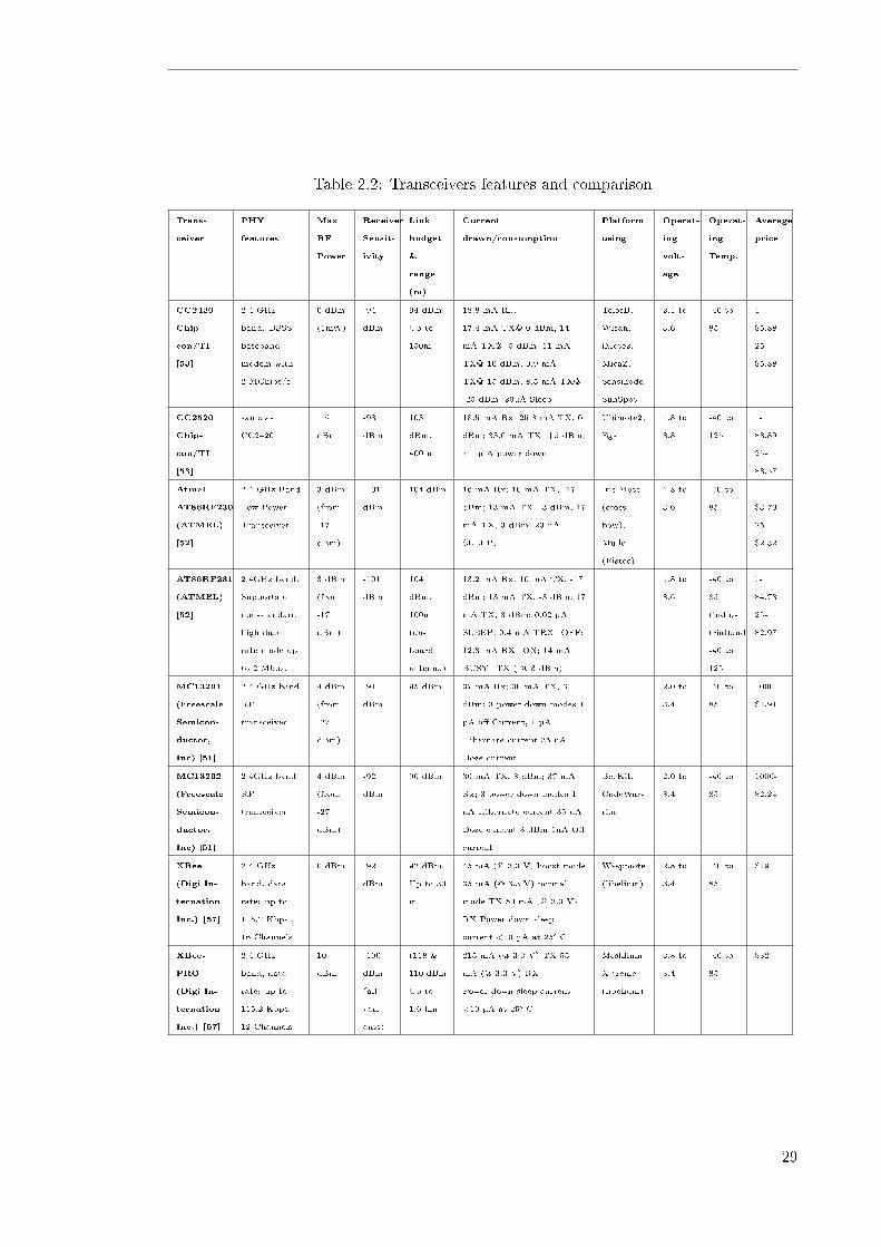
Table 2.2: Transceivers features and comparison
Trans-
ceiver
PHY
features
Max
RF
Power
Receiver
Sensit-
ivity
Link
budget
&
range
(m)
Current
drawn/consumption
Platform
using
Operat-
ing
volt-
age
Operat-
ing
Temp.
Average
price
CC2420
Chip-
con/TI
[53]
2.4 GHz
band. DSSS
baseband
modem with
2 MChips/s
0 dBm
(1mW)
-94
dBm
94 dBm.
Up to
150m
18.8 mA Rx;
17.4 mA TX@ 0 dBm; 14
mA TX@ -5 dBm; 11 mA
TX@-10 dBm; 9.9 mA
TX@-15 dBm; 8.5 mA TX@
-25 dBm; 20µA Sleep
TelosB,
Wisan,
iMote2,
MicaZ,
Sensinode,
SunSpot
2.1 to
3.6
-40 to
85
1-
$5.88
25-
$5.88
CC2520
Chip-
con/TI
[53]
same as
CC2420
+5
dBm
-98
dBm
103
dBm.
400 m
18.5 mA Rx; 25.8 mA TX, 0
dBm; 33.6 mA TX, +5 dBm;
<1 µ A power down
Ubimote2,
Egs
1.8 to
3.8
-40 to
125
1-
$3.89
25-
$3.57
Atmel
AT86RF230
(ATMEL)
[52]
2.4 GHz Band
Low Power
Transceiver
3 dBm
(from
-17
dBm)
-101
dBm
104 dBm 16 mA Rx; 10 mA TX, -17
dBm; 13 mA TX, -3 dBm; 17
mA TX, 3 dBm; 20 nA
SLEEP;
Iris Mote
(cross-
bow),
Mulle
(Eistec)
1.8 to
3.6
-40 to
85
1-
$3.70
25-
$2.32
AT86RF231
(ATMEL)
[52]
2.4GHz band.
Supports a
non-standard
high data
rate mode up
to 2 Mbps.
3 dBm
(from
-17
dBm)
-101
dBm
104
dBm.
100m
(on-
board
antenna)
13.2 mA Rx; 10 mA TX, -17
dBm; 13 mA TX, -3 dBm; 17
mA TX, 3 dBm; 0.02 µA
SLEEP; 0.4 mA TRX_OFF;
12.3 mA RX_ON; 14 mA
BUSY_TX ( @ 3 dBm)
1.8 to
3.6
-40 to
85
(indus-
trial)and
-40 to
125
1-
$4.73
25-
$2.97
MC13201
(Freescale
Semicon-
ductor,
Inc) [51]
2.4 GHz band
RF
transceiver
4 dBm
(from
-27
dBm)
-91
dBm
95 dBm 37 mA Rx; 30 mA TX, 3
dBm; 3 power down modes 1
µA o� Current, 1 µA
Hibernate current 35 uA
Doze current
2.0 to
3.4
-40 to
85
1000-
$1.91
MC13202
(Freescale
Semicon-
ductor,
Inc) [51]
2.4GHz band
RF
transceiver
4 dBm
(from
-27
dBm)
-92
dBm
96 dBm 30 mA TX, 3 dBm; 37 mA
Rx; 3 power down modes 1
uA Hibernate current 35 uA
Doze current 3 dBm 1uA O�
current
BeeKit,
CodeWar-
rior
2.0 to
3.4
-40 to
85
1000-
$2.24
XBee
(Digi In-
ternation
Inc.) [57]
2.4 GHz
band, data
rate: up to
115.2 Kbps ,
16 Channels
0 dBm -92
dBm
92 dBm.
Up to 30
m
45 mA (@ 3.3 V) boost mode
35 mA (@ 3.3 V) normal
mode TX 50 mA (@ 3.3 V)
RX Power-down sleep
current <10 µA at 25° C
Waspmote
(libelium)
2.8 to
3.4
-40 to
85
$19
XBee-
PRO
(Digi In-
ternation
Inc.) [57]
2.4 GHz
band, data
rate: up to
115.2 Kbps,
12 Channels
10
dBm
-100
dBm
(all
vari-
ants)
(118 &
110 dBm
Up to
1.6 km
215 mA (@ 3.3 V) TX 55
mA (@ 3.3 V) RX
Power-down sleep current
<10 µA at 25° C
Meshlium
X treme
(libelium)
2.8 to
3.4
-40 to
85
$32
29

a�ect the battery capacity [58]. Given the battery capacity of a particular battery, and
by �nding the average current drained by the system, we can approximately obtain the
battery life span using the following expression:
CapacityIpavg
For example, given the battery capacity of 2850mAh and average drained current of
11.623mA, the expected battery life time is approximately 245.19 hours if running contin-
uously.
2.4 Current State of Wireless Networks Deployment
Despite the wide use of the 802.11 standards for wireless communication , various studies
have observed degradation in performance when the IEEE 802.11 standard is used in
distributed network scenarios [59, 60]. These studies found the IEEE 802.11 medium
access control (MAC) protocols inability to perform well in such environments in terms of
energy e�ciency and other performance parameters. These �ndings alerted future research
to look at the MAC schemes that will be suitable for wireless sensor network operating in
a multi-hop mode without excessive performance degradation. However, one cannot ignore
the fact that the exploding success of wireless area networks (WLANs) over recent years,
especially in commercial based applications, is due to the products that are based on IEEE
802.11 standard. The IEEE 802.11 standard is well established and has won the market
place of wireless networked devices at relatively low prices. Most likely, future standards
will still operate in coexistence with the 802.11 networks and also other technologies [59].
The new standards such as the IEEE 802.15.1 (Bluetooth) and 802.15.4 (ZigBee) standards
are currently receiving more attention in the development of wireless sensor applications
[61, 42, 62].
Choi [61] suggests the use of bluetooth standard for security system wireless sensor network.
However, Heng-Chih [62] made a comparison between Bluetooth and ZigBee showing as
the latter being more energy e�cient and therefore a more appropriate solution for long
operation time sensor networks. Furthermore he argues that bluetooth has several other
limitations compared to ZigBee that include high-cost, longer latency, and low density.
Table 2.3 shows some of the standards in comparison to the IEEE 802.15.4 standard.
30

Geer [42] quoted a research vice president at Gartner Dataquest, a market research �rm,
predicted that a worldwide increase in number of devices connected via ZigBee from 400,000
in year 2005 to 150 million in 2010 as shown in �gure 2.2.
Table 2.3: A comparison between 802.15.4 and other standards
The greatest challenge is developing e�ective WSN communication systems that will run
unattended for years from a limited energy resource. This requires both energy-e�cient,
robust hardware and an e�cient software management system. We expect the emerging
WSNs to be more energy-e�cient with reliable connectivity, given that the compactness
and increasing density of new wireless devices impose greater constraints on battery capac-
ities and connectivity. To minimize the power loss in a node, system components must be
optimized and be compatible with e�cient algorithms or protocols without a�ecting the
target application requirements, e.g, saving energy [22, 26]. Furthermore, the design must
be cost e�ective in terms of hardware costs, communication e�ciency and the complete
cost equation including development costs and product life cycle support costs. While
technology is still emerging, progress has not been as rapid as predicted. Instead of smart
dust sprinkles from aircraft, we have large nodes connected by myriad wires to transducers
[4]. Researchers are still concerned with networking and maximizing the lifetime of net-
works powered by �nite electrochemical primary cells. While energy considerations have
dominated most WSN research, the increasing interest in real-time applications involving
31
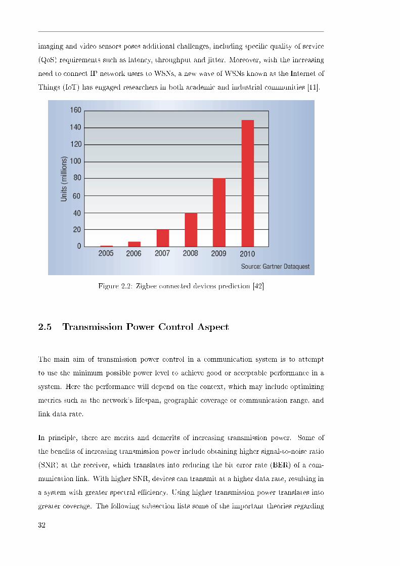
imaging and video sensors poses additional challenges, including speci�c quality of service
(QoS) requirements such as latency, throughput and jitter. Moreover, with the increasing
need to connect IP network users to WSNs, a new wave of WSNs known as the Internet of
Things (IoT) has engaged researchers in both academic and industrial communities [11].
Figure 2.2: Zigbee connected devices prediction [42]
2.5 Transmission Power Control Aspect
The main aim of transmission power control in a communication system is to attempt
to use the minimum possible power level to achieve good or acceptable performance in a
system. Here the performance will depend on the context, which may include optimizing
metrics such as the network's lifespan, geographic coverage or communication range, and
link data rate.
In principle, there are merits and demerits of increasing transmission power. Some of
the bene�ts of increasing transmission power include obtaining higher signal-to-noise ratio
(SNR) at the receiver, which translates into reducing the bit error rate (BER) of a com-
munication link. With higher SNR, devices can transmit at a higher data rate, resulting in
a system with greater spectral e�ciency. Using higher transmission power translates into
greater coverage. The following subsection lists some of the important theories regarding
32

multi-hop TPC, namely, connectivity and topology maintenance; spatial reuse and detec-
tion; and energy consumption. A multi-hop wireless sensor network is de�ned as a network
whereby a packet may have to traverse multiple consecutive wireless links in order to reach
the destination [63].
2.5.1 Connectivity and Topology Maintenance
The network topology depends on a number of controllable and noncontrollable factors.
Some of noncontrollable factors include node mobility, weather, interference and noise.
Some of the controllable factors include transmit power and antenna direction. Topology
maintenance aims to reduce transmission range by adjusting the nodal radio transmis-
sion range downward while maintaining necessary network properties such as connectivity
[64, 35]. A network is constructed having network connectivity whereby each node can
communicate with any other nodes in the network, via single a hop or via multiple hops.
By minimising transmission power, we control the network topology by reducing the num-
ber of links (depending on the network density). If the transmit power is too low, the
network might be disjointed, and if we transmit at excessively high power then we use
energy ine�ciently and cause interference in the shared radio channel. Topology control
aims to minimize the number of links that constitute the topology. Power control in terms
of topology maintenance, retention of connectivity, reduces power consumption and also
reduces MAC level interference. However, as transmission power decreases or carrier sense
threshold increases the signal to interference ratio, SINR also decreases as a result either
of smaller received signal or an increased interference level. In terms of connectivity then
the optimal common transmission power will be power just su�cient to preserve network
connectivity [65].
2.5.2 Spatial Reuse and Detection Advantages
The spatial reuse in the case of a wireless network is the network's ability to allow multiple
communication to proceed simultaneously [66]. In the physical layer, one can increase the
level of spatial reuse to possibly allow higher throughput by either reducing the transmit
power or reducing the carrier sense range by an increase in the carrier sense threshold
(CSthresh_). In [67] it was found that spatial reuse depends on the ratio of transmission
power and carrier sense threshold. Even though spatial reuse characterise the performance
33

of MAC by determining the number of simultaneous communication to proceed, here it
shows the need for cross layer improvement since this can be controlled at the physical
layer.
2.5.3 Multi-hop and Energy Consumption
Some of the previous research suggest that multi-hop communication in densely deployed
sensor networks is expected to consume less power than traditional single hop commu-
nication [31, 32, 33]. So if we can use minimum possible power while still maintaining
connectivity, we can reduce the energy consumption, Joule/byte transmitted and therefore
prolong the lifespan of wireless sensor nodes [68, 67, 33, 32]. Zhao [31] suggests that an N
hop multi-hop communication can be more energy-e�cient than single-hop communication
for same distance, Nr by deriving the following expression:
ηrf = Psend(Nr)N.Psend(r)
= (Nr)αPreceivedN.rαPreceived
= Nα−1
where r , α, Psend, and Preceived are the one-hop distance, radio frequency (RF) attenuation,
the power at a transmission node, and the minimum received power at a node respectively.
2.6 A Review on Wireless Medium Access Control Protocols
Data link layer is responsible for establishing a reliable and secure logical link over the
unreliable wireless link. The data link is therefore responsible for wireless link error con-
trol, security(encryption or decryption), mapping network layer packets into frames, and
packet retransmission. A sublayer of the data link layer is known as the media access
control (MAC) protocol layer. Like in all shared medium networks, medium access control
is responsible for coordinating the access of active nodes or users in the communication
channel or channels. Figure 2.3 shows the MAC categories. When dedicated channels
are allocated to users it is often called multiple access. Bandwidth sharing using random
channel allocation is known as random multiple access or simply random access. All ran-
dom access techniques use some sort of carrier sensing, such as the carrier sense multiple
access with collision detection (CSMA/CD) which is used in the wired IEEE802.3 stan-
dard (Ethernet) similar to carrier sense multiple multiple access with collision avoidance
34

(CSMA/CA) described in section 2.13 used in wireless networks such as WPAN, WLAN
and ALOHA [69, 21]. All active users contend for the channel, hence this MAC scheme is
sometimes known as a contention based scheme. The Distributed Coordination Function
(DCF) of the IEEE802.11 standard [8] and the Contention Access Period (CAP) of the
IEEE 802.15.4 standard [7] are good examples of contention based protocols.
In general, the choice of whether to apply a particular multiple access or a particular ran-
dom access will depend on several factors. Some of these basic factors include the system
application, the nature of tra�c characteristics of the users in the system, the performance
requirements, characteristics of the channels and other interfering systems operating in the
same bandwidth. Traditionally, wireless channel access schemes can be classi�ed into two
broad categories namely random based or contention based and reservation or dedicated or
contention-free based. The channel access schemes are sometimes classi�ed based on their
operating principle, for example contention based access mechanism is sometimes referred
to as the decentralized or distributed medium access scheme and the centralized mecha-
nisms that use techniques such time-division multiple access (TDMA), frequency division
multiple access (FDMA), code division multiple access (CDMA) or hybrid combination of
these reservation based channel accesses. An example of reservation based channel access
is that of Point Coordination Function (PCF) of IEEE 802.11 that employs polling.
Applications with continuous transmission and delay constraints, such as voice or video,
typically require dedicated channels for good performance to ensure their transmission is
not interrupted. However, most data users, or in particular sensor networks, do not require
continuous transmission. i.e. data is generally generated at random time instances, and
therefore dedicated channel assignment can be extremely ine�cient. Furthermore, most
network scenarios have a total number of users that are active users plus idle users than can
be accommodated simultaneously, so at any given time channels should only be allocated
to users or nodes that need them. Therefore, random access protocols are more e�ective
with burst tra�c where there are many more users than available channels, and when
these uses rarely transmit. On the other hand if the users have long strings of packets or
continuous streaming data, then random access works poorly as most transmission results
in collisions. In such cases performance can be improved by assigning channels to users in
a more systematic fashion using one of the dedicated or scheduling channel schemes.
Contention based access schemes are usually used for ad-hoc wireless networks due to their
distributive nature, simplicity and lack of synchronization requirements. However, each
35
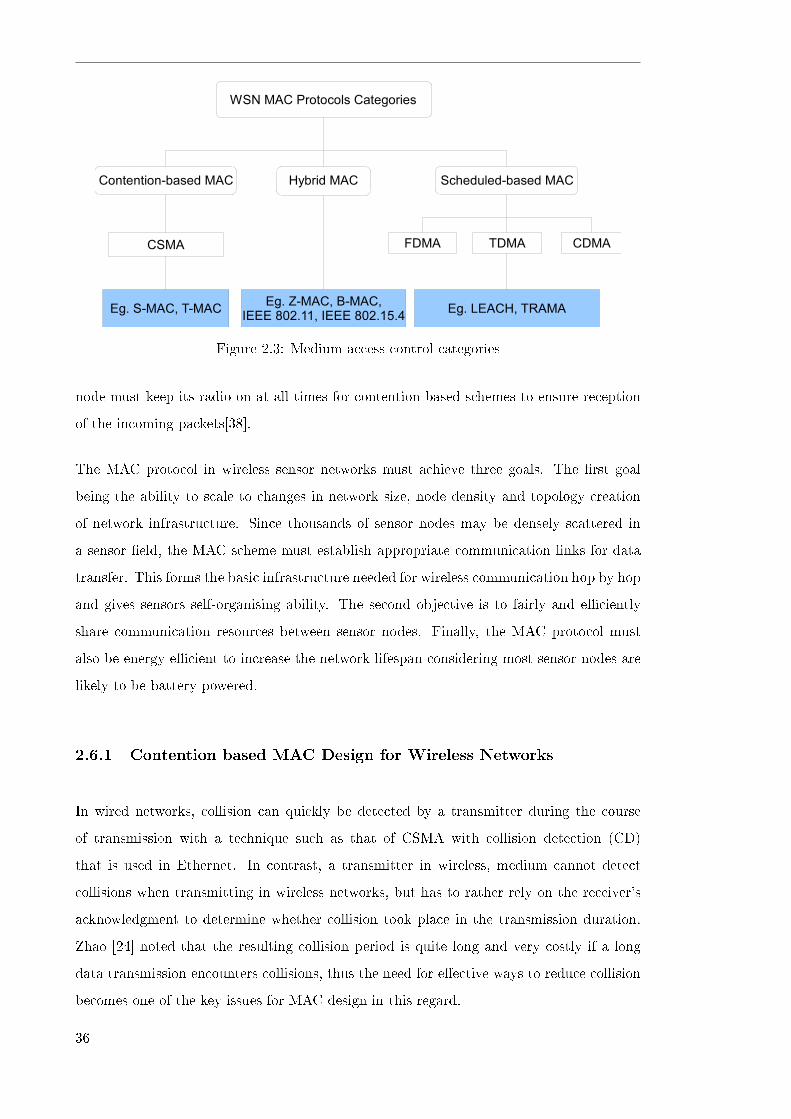
Figure 2.3: Medium access control categories
node must keep its radio on at all times for contention based schemes to ensure reception
of the incoming packets[38].
The MAC protocol in wireless sensor networks must achieve three goals. The �rst goal
being the ability to scale to changes in network size, node density and topology creation
of network infrastructure. Since thousands of sensor nodes may be densely scattered in
a sensor �eld, the MAC scheme must establish appropriate communication links for data
transfer. This forms the basic infrastructure needed for wireless communication hop by hop
and gives sensors self-organising ability. The second objective is to fairly and e�ciently
share communication resources between sensor nodes. Finally, the MAC protocol must
also be energy e�cient to increase the network lifespan considering most sensor nodes are
likely to be battery powered.
2.6.1 Contention based MAC Design for Wireless Networks
In wired networks, collision can quickly be detected by a transmitter during the course
of transmission with a technique such as that of CSMA with collision detection (CD)
that is used in Ethernet. In contrast, a transmitter in wireless, medium cannot detect
collisions when transmitting in wireless networks, but has to rather rely on the receiver's
acknowledgment to determine whether collision took place in the transmission duration.
Zhao [24] noted that the resulting collision period is quite long and very costly if a long
data transmission encounters collisions, thus the need for e�ective ways to reduce collision
becomes one of the key issues for MAC design in this regard.
36

Several techniques can be used to control collision in random medium access, namely carrier
sense, handshaking and backo� mechanisms [70]. Carrier sense requires the transmitter to
transmit only when the channel is determined to be idle. Handshaking between transmitter
and receiver, which involves an exchange of short frame packets between transmitter and
receiver before transmitting data packets to avoid long collision periods of data packets.
Furthermore, the backo� mechanism described in section 2.13 forces each node to wait for
a random period before attempting retransmission to avoid collision.
2.7 MAC Power Consumption Sources
The sources of power consumption in wireless sensor networks can be classi�ed into two
types: communication related and computation related. The understanding of power char-
acteristics of the mobile radio used in wireless devices is important for an e�cient design
of communication protocols. Unlike wired networks for which the topology is �xed except
in the cases of link failures, WSN have dynamic topologies based on the location of the
sensor nodes and their range of transmission. For su�ciently dense networks, nodes can
restrict communication only to nearby nodes with reduced range of transmission and yet
maintain global network connectivity. The mechanism for computing the su�cient trans-
mission ranges for each node is known as topology control, and its main goal is to optimise
performance in terms of network lifetime and throughput while maintaining a connected
network.
A typical mobile radio may exist in three modes namely: transmit, receive, and standby.
Maximum power being used while transmitting and the least power usage occurs during
the standby mode. Since the MAC-layer is responsible for allocating the medium so that
multiple units do not interfere with each other's transmissions, it is no coincidence that
some power saving optimisations need to be looked at in this particular layer. Previous
research into MAC layer power optimisation have been investigating four possible ways
to reduce power consumption in wireless networks. These include reducing sending time,
reducing power while sending, reducing listening time, and reducing switching time.
37

2.8 MAC Protocols - Related Work
The medium access control is a broad research area, and a good number of researchers
have worked in the area of power e�cient MACs and wireless sensor networks [71, 18, 72].
One of the pioneers in the area of power e�cient MAC protocols is PAMAS, which tries to
reduce the overhearing between nodes by using a separate signalling channel [73]. However
this requires an extra radio and therefore increases the cost and complexity of sensor nodes.
Another MAC known as PCM (Power Control MAC) and PCM does not use a separate
signalling channel like PAMAS [74]. This MAC protocol is an extension to the standard
IEEE 802.11 MAC protocol, and it can be used by any protocol applying CSMA/CA.
The main goal of the PCM is to use less power compared to the 802.11 standard and still
retain the same throughput. It does this by transmitting DATA and ACK at minimum
possible power and transmitting RTS and CTS at maximum power. To reduce collisions,
data transmissions are periodically transmitted at maximum power, so that neighbours
can sense the medium as occupied, and refrain from sending RTS packets.
S-MAC is a contention based MAC protocol like IEEE 802.11. This protocol uses a number
of techniques to reduce energy consumption by close to 50 percent compared to 802.11 and
still maintain a tolerable latency and throughput [18]. In S-MAC all nodes in the network
synchronize their respective sleep or wake schedules, and all nodes that maintain the same
schedule belong to the same virtual cluster (neighbouring nodes). The main di�erence
between S-MAC and IEEE 802.11 in power save mode is that the latter is designed for single
hop networks, whereas S-MAC includes synchronisation between the nodes in the network.
S-MAC adds power saving features to the virtual carrier sense. When NAV is nonzero,
and the ongoing transmission does not involve the current node, the radio is powered o�
or down until the NAV reaches zero. The design reduces the energy consumption caused
by idle listening and tackles the overhearing problem by sending to sleep interfering nodes
once they hear RTS/CTS. However, this design embodies or activates a trade o� of latency
as latency is increased, since sender nodes must wait for the receiver to wake up before
sending out data [18]. Wei's [18] main goal in the design of the S-MAC protocol was
to reduce energy consumption, while supporting scalability and collision avoidance. He
identi�es and describes the causes of energy waste that include idle listening, collisions,
overhearing, and control overhead. S-MAC is not only a link protocol, but also a network
and organisation protocol. The S-MAC design involves synchronisation that consumes
energy and TDMA complexity may not be suitable for simple devices.
38

T-MAC (Timeout MAC) [75] is another contention-based MAC protocol with a/the main
design goal to reduce energy consumption. T-MAC improves S-MAC's energy usage by
allowing active nodes to have adaptive or variable duty-cycles rather than �xed ones. The
design allows every node to decide its own duty-cycle based on its activation period. T-
MAC protocol ends the active time by timing out on hearing nothing for a period known as
timeout. The T-MAC protocol has more latency compared to an S-MAC protocol; however
it gives much better energy performance for low data rate applications. The design of T-
MAC � similar to S-MAC � also uses periodic time synchronisation that consumes much
energy.
B-MAC (Berkeley MAC) [76] is another contention-based MAC protocol where the main
design goal is to reduce energy consumption, and with an additional goal of keeping the
implementation simple with small code and RAM size. B-MAC carrier sensing uses Clear
Channel Assessment (CCA) with the sleep or wake scheduling using Low Power Listening
(LPL). B-MAC is only a link protocol with network services such as organisation, synchro-
nisation, and routing built above its implementation needs[76]. B-MAC design provides
an interface to the user to change di�erent parameters such as CCA, acknowledgments,
back-o�s and LPL to suit a particular WSN application scenario at run-time. The design
emphasis is on keeping the code size small and on providing complete �exibility. Another
advantage of this design is that no RTS/CTS and synchronisation packets are required.
However, the design causes or creates huge overhead because of overhearing, whereby re-
ceiver nodes have to keep themselves on for receiving a long preamble even though they
might not be the intended destination.
Z-MAC (Zebra MAC) [77] is a hybrid MAC scheme that combines the strength of CSMA
and TDMA. With Z-MAC, nodes within interference range transmit during di�erent times,
so as to be collision free, however unlike TDMA, a node can transmit during any given time
slot. The main design goal of the T-MAC is to reduce energy consumption by preventing
collision caused by hidden nodes, and to control overhead such as RTS/CTS or Data/ACK.
2.9 IEEE 802.15.4 Overview
An increased attention in WSN applications has triggered the development of standard
protocols speci�cally designed for intended range of applications. Among other develop-
ment, is the recently proposed IEEE 802.15.4 standard, which describes the Physical layer
39

(PHY) and medium access control (MAC) sublayer speci�cations for wireless communica-
tion standard particularly for low-rate, low-power consumption wireless personal area net-
works (LR-WPANs). Since the introduction of 802.15.4 standard for wireless personal area
network (WPAN) in 2003 by the IEEE 802.15 working group, WPAN has tremendously
attracted research and development in wireless sensor networks (WSNs). The standard
has been designed to provide low complexity, low cost and low power wireless connectivity,
which makes it one of the most anticipated technologies enabling wireless sensor networks
(WSNs).
2.10 IEEE 802.15.4 Physical Speci�cation
The IEEE 802.15.4 physical layer is responsible for data transmission and reception using a
certain radio channel and according to speci�c modulation or demodulation and spreading
or de-spreading technique. The standard also provides other common provisions such as
receiver sensitivity, the ability to adjust transmitter power, ability to dynamically select
channel, a channel scan function in search of a beacon, activation and deactivation of radio
transceiver, ability to measure received packet energy known as energy detection (ED) ,
the ability to measure the quality of the received signal for each packet known as link
quality indicator (LQI) and the ability to check for activity in the medium known as clear
channel assessment (CCA).
IEEE 802.15.4 network may operate in one of the three Industrial, Scienti�c, Medical (ISM)
frequency bands: 2.45GHz, 915MHz and 868MHz as illustrated in �gure 2.4 . There is a
single channel between 868 and 868.6 MHz in the 868MHz band, 10 channels between 902
and 928MHz in the 915MHz band, in 2 MHz steps, numbered 1 through 10 and 16 channels
between 2.4 and 2.4835GHz in 2.45GHz band, in 5 MHz steps, numbered 11 through 26.
The center frequency of these 27 channels in three frequency bands is de�ned as follows:
Fc = 868.3MHz, for k = 0
Fc = 906 + 2 (k − 1)MHz, for k = 1, 2, ..., 10
Fc = 2405 + 5 (k − 11)MHz, for k = 11, 12, ..., 26
where k is the channel number.
40

Figure 2.4: IEEE 802.15.4 frequency spectrum
The standard uses direct sequence spread spectrum (DSSS) as a spreading technique for
all bands. Frequency bands 868MHz and 915MHz utilise DSSS with a comparatively low
chip rate as a spreading technique and binary phase shift keying (BPSK) modulation,
which result in maximum attainable data rates of 20 kbps and 40 kbps, respectively. The
2.45GHz band uses a 16-ary quasi-orthogonal modulation technique is used, in which four
data bits comprise one modulation symbol and the chip sequence is then modulated onto
the carrier using o�set quadrature phase shift keying (O-QPSK),attaining data rate of up
to 250 kbps (Table 2.4).
We use the 2.45GHz frequency band in this research for three reasons. Firstly, since it
provides high radio data rate (250kb/s) which reduces the frame transmission time and
therefore reduces the energy per transmitted and received bit. Secondly, because network
scalability is improved given that a large number of nodes may communicate with each
other within a time period, and lastly, because the band is available in most countries
worldwide.
2.10.1 Channel Frequency Selection
The PHY layer should be able to tune its transceiver into a speci�c channel requested by
upper layers. Dynamic channel selection (DCS) involves a number of procedures to enable
802.15.4 devices to change their radio channel based on measurements and regulatory
41

Table 2.4: IEEE 802.15.4 physical parameters
PHY
(MHz)
Frequency
bands
(MHz)
ChannelsData parameters Spreading parameters
Bit
rate
(kbps)
Symbol
rate
(ksymbol-
s/s)
Data
Modula-
tion
Chip
rate
(kchip/s)
Chip
Modula-
tion
868/915868 - 868.6 1 20 20 BPSK 300 BPSK
902 - 928 10 40 40 BPSK 600 BPSK
24502400 -
2483.516 250 62.5 16-ary
Orthogo-
nal
2000 O-QPSK
requirements. When a node �rst associates with the network, the association frame includes
a supported channels information element, which reveals the channels supported by the
station. The selection of a particular channel can a�ect the initial association procedure
and ongoing network operations [78, 79, 80]. DCS will periodically test the channel for
potential interference from other radio systems by stopping the transmission on the network
and measuring potential interference, and if necessary communicating the need for channel
change.
2.10.2 Receiver sensitivity and capture threshold
The receiver threshold value or receiver sensitivity is the signal power required to achieve
a particular BER or is the least power level of a packet for its transmission to be detected
successively; if the received signal power is lower than RXthreshold, it cannot be detected
successfully. For example, when a node is presently receiving a packet of power Pa, and
a packet at power level Pb arrives, the following comparison must be made to determine
whether or not capture occurs:
10log (Pa)− 10log (Pb) > 10db or PaPb> 10
Receiver sensitivity is measured in dBm, whereby 0 dBm equals 1mW, and power below
1mW are expressed as negative number. For example 0.01 mW would be -20 dBm. There-
fore, the lower the power level that the receiver can successfully process, the better the
receiver sensitivity [81, 67]. Rxthreshold depend on a function of modulation used, and
packet size. For small packets even -80dBm(1x10⁻¹¹W ) is enough, however receiver sen-
sitivity of -85 or better is preferably. For simulation purposes, NS-2 threshold.cc can be
used to calculate the value of RXthreshold required for a particular receiver range [82].
42

However this does not necessary mean there exists a physical card with such value of RX
and CS thresholds.
Transmission range of a mobile node can also be changed in the tcl script by simply
changing the receiving threshold with the following command line:
Phy/WirelessPhy set RXThresh_ <value>
For any given receiver, the higher the data rate, the less sensitive will be the receiver, since
more power is required at the receiver to support higher data rates. For example, a receiver
sensitivity of -98 dBm is better than a receive sensitivity of -95 dBm by 3 dB, or a factor
of two. In other words, at a speci�ed data rate, a receiver with a -98 dBm sensitivity can
hear signals that are half the power of those heard by a receiver with a -95 dBm receiver
sensitivity.
2.10.3 Receiver Energy Detection (ED)/Digital RSSI
Receive Signal Strength Indicator (RSSI) is a transceiver's feature which is able to estimate
or indicate Radio Frequency (RF) strength (power) of an incoming signal at the receiving
antenna. The RSSI is derived from received signal strength as ratio of received power to
the reference power (Pref ). Typically, the reference power represents an absolute value of
Pref = 1mW.
RSSI = 10logPrPref
[RSSI] = dBm (2.2)
Before a device can transmit a message, it �rst goes into receive mode to detect and estimate
the received signal power (energy level) within the bandwidth of a current channel. This
task is known as energy detection (ED). The ED time is equal to 8 symbol periods, and
the signal energy in the band of interest is averaged over this period. Most of embedded
devices such as telosb, CC2420 has a built-in RSSI yielding a digital value that can be read
from the 8 bit, signed 2's complement RSSI_value register. This value is always averaged
over 8 symbol periods (128µs @250 kbps), in accordance with the IEEE 802.15.4 standard
[50].
43

Receiver's ED does not attempt to detect the signal type but rather the signal energy level
estimated (i.e., ED does not reveal as to whether the signal is an IEEE 802.15.4 standard
compliant or not). In addition, ED might not be able to detect weak signals with energy
level close to receiver sensitivity level. The MAC request the PHY to perform ED, then the
ED results will be reported to the MAC (MLME) using PLME-ED.con�rm, which return
an 8-bit integer indicating energy level in the frequency channel of interest [7].
2.10.4 Link Quality Indicator (LQI)
A link quality indicator (LQI) indicates the signal strength and/or quality of packets
received by the receiver. The received signal strength (RSS) is a measure of the total
energy of the received signal, this can be determined using receiver ED. Another way of
looking at signal quality is by using a signal to noise ratio (SNR) estimation (where higher
SNR is considered a higher quality signal, and so forth). Therefore, LQI measurement may
be implemented using receiver ED, a signal-to-noise estimation, or a combination of both
methods.
The LQI measurement is performed for each received packet and the result reported to
the MAC sublayer using PD-DATA.indication, which return an integer ranging from 0x00
to 0x�. The link quality that is received by higher layers is simply the RSSI value (in
dBm) after it has been scaled and o�set. This is done to get the value in the 0-255 range
rather than the -40 to -95 range typical of RSSI values. The conversion can be found
in a mac_radio_defs.h �le, de�ned as MAC_RADIO_CONVERT_RSSI_TO_LQI(x).
The value of LQI relates to RSSI value in a linear function. The LQI works in the same
way as the ED, except that LQI is measured over 64µs period after the incoming packet
preamble[78]
2.10.5 Carrier Sensing (CS) and Clear Channel Assessment (CCA)
Similar to ED, carrier sense (CS) is a method used to verify as to whether a frequency
channel is available to use. Before a device can transmit a message, it goes into the
receive mode to detect the type of any possible signal that might be present in the desired
frequency channel. In contrast to ED, in CS, the signal is demodulated to verify whether
the signal modulation and spreading are compliant with the characteristics of the PHY
44
that is currently in use by the device. If the occupying signal is compliant to IEEE 802.15.4
PHY, the device might choose to consider the channel busy regardless of the signal level.
The Carrier sense threshold (CSthreshold) provides the sensing range of the nodes. CSthresh-
old value is used by medium access control (MAC), when a node senses the channel and
�nd that the sampled energy or received power is below CSthreshold, the node will perceive
the channel to be idle.
The concept of CCA was �rst proposed as an enhancement ALOHA. CCA is a physical
layer activity and is an essential element of the CSMA protocol.The CCA provides two
important services: (i) detecting an incoming packet, (ii) ensuring a free channel before
transmission. The CCA module processes received radio signals in a suitable time termed
CCA window. The CCA processing can be either energy detection or sense of speci�c
features of signal over the channel. It then reports channel state, either busy or idle, by
comparing the detection with a threshold.
The 802.15.4 PHY provides the capability to perform clear channel assessment (CCA) to
determine whether the channel is busy or idle by comparing the energy in the channel with
a threshold. The CCA is part of the PHY management service. In CSMA/CA channel
access mechanism, the MAC request the PHY to perform a CCA to ensure that the channel
is not in use by any other device. The 802.15.4 compliant PHY perform CCA according
to at least one of the following methods:
� Mode 1: Energy above threshold. CCA will report a busy channel if it detects energy
above the energy detection (ED) threshold. Whereby, the ED threshold will be at
most 10 dB above the speci�ed receiver sensitivity.
� Mode 2: Carrier sense only. CCA will report a busy channel if it detects a signal with
comparable modulation and spreading characteristics of IEEE 802.15.4 transmission,
regardless of signal's energy being above or below the ED threshold.
� Mode 3: Carrier sense with energy above the threshold. CCA will report a busy
channel only if it detects a signal with comparable modulation and spreading char-
acteristics of IEEE 802.15.4 transmission with energy above the ED threshold. This
is a combination of the two modes above.
The MAC request is received by the PLME-CCA.request primitive (see subsection 2.10.7)
during reception of a PHY protocol data unit (PPDU). A busy or idle channel will be
45

indicated by the PLME-CCA.con�rm primitive with status BUSY or IDLE respectively.
The CCA detection time will be equal to eight symbols periods. The PHY PIB attribute
phyCCAmode will indicate the appropriate CCA operation mode(1-3).
MAC uses physical carrier sensing (PCS) whenever a node intend to start transmitting a
packet. PCS is performed at the physical layer whereby the medium is sensed before a node
initiate transmission. Similarly, 802.15.4 uses clear channel assessment (CCA) or energy
detection provided as received signal strength indicator (RSSI) services in 802.15.4 PHY.
Figure �shows the CSMA/CA algorithm used by the MAC layer. The node will transmit
a packet only when the energy level of the RF medium signal sampled by PCS is below
the carrier sense threshold. Consequently, PCS plays an important role in MAC layer
collision avoidance algorithm. Usually the PCS threshold is a static constant value in most
MAC implementation [83, 81]. We can minimise collision and interference if we properly
tune carrier sensing PCS threshold [83], in doing so, we conserve energy as well. Higher
value of PCS threshold (CSthresh_) would lead into more collision due to hidden terminal
problem and lower value would decrease the level of spatial reuse. Currently most of PCS
are con�gured with �xed very low values that sometimes even a remote communication
would generate a signal strong enough to make a station withhold its transmission, as a
result very little spatial reuse is possible. Liu [81]argues that independent variable PCS are
not suitable for WSNs due to sensor nodes energy limitations and processing capability.
An analytical model for deriving an optimal carrier sense threshold for the IEEE 802.11
mesh network is presented by Zhu[83].
2.10.6 PHY Frame Format
The PHY protocol data unit (PPDU) packet is illustrated in Figure 2.5. Each PPDU
packet consists of the following basic components:
� A synchronization header (SHR), which allows a receiving device to synchronize and
lock into the bit stream. This consists of four bytes of zeros preamble �eld used for
synchronisation and one byte of a prede�ned start-of-frame delimiter (SFD) used to
indicate the end of synchronisation and the start of the data packet.
� The PHY header (PHR), which contains frame length information (from 0 to 127
bytes, inclusive).
46

� The PHY service data unit (PSDU) which carries the MAC sublayer frame of variable
length.
Figure 2.5: IEEE 802.15.4 frame format
2.10.7 Physical Service Speci�cations
The PHY layer provides an interface between the MAC sublayer and the physical radio
channel, via the RF hardware (Figure 2.6). The PHY layer conceptually includes a man-
agement entity called the PLME, which provides the layer management services interfaces
through which layer management functions may be invoked. The PLME is also responsible
for maintaining the PHY layer database known as the PHY PAN information base (PIB),
containing PHY managed objects.
PHY provides two services that can be accessed through two Service Access Points (SAPs).
These are the PHY data service, accessed through the PHY data SAP (PD-SAP), and the
PHY management service, accessed through the PLME's SAP (PLME-SAP).
The standard de�nes ways through which communication is carried between layers via
service primitives having the following form:
� Request-a layer uses this type of primitive to request that another layer perform a
speci�c service.
� Con�rm-a layer uses this type of primitive to convey the results of a previous service
request primitive.
� Indication-a layer uses this type of primitive to indicate to another layer that a
signi�cant event has occurred. This primitive could result from a service request or
from some internally generated event.
47

� Response-a layer uses this type of primitive to complete a procedure initiated by an
indication primitive.
The PD-SAP which supports exchange of data packets between MAC and PHY has the fol-
lowing primitives: PD-DATA.request, PD-DATA.con�rm and PD-DATA.indication. The
PLME-SAP which support the exchange of management commands between MLME and
PLME has request and con�rm primitives for the followings: PLME-CCA, PLME-ED,
PLME-GET, PLME-SET-TRX-STATE and PLME-SET. These primitives are an abstract
way of de�ning the protocol, and they do not imply a speci�c physical implementation
method. Similarly, the MAC layer provides an interface between network or application
layer.
Figure 2.6: PHY layer and MAC sublayer reference model
There are several constants that de�ne characteristics of a particular PHY layer; these con-
stants are hardware dependent and therefore cannot be changed during operation. These
constants variables include:
� aMaxPHYPacketSize, which is the maximum PSDU packet size the PHY will be able
to receive is 127 bytes, and
� aTurnaroundTime, which is the RX-to-TX or TX-to-RX 12 symbol periods maximum
turnaround time.
There are also several variable attributes in PHY PIB required to manage a device's PHY
layer. These attributes can be read or written using PLME-GET.request and PLME-
SET.request primitives, respectively. These attributes include:
48

� phyCurrentChannel, which is the desired RF channel out of 27 valid channels to be
used for transmissions and receptions
� phyChannelsSupported, which is the supported channel or channels amoung 27 valid
channels
� phyTransmitPower, which is thedi�erent power levels
� phyCCAMode, which is the CCA mode used out of the three CCA modes
2.11 Supported Network Devices
In the IEEE 802.15.4 speci�cations, network devices can be classi�ed as full-function
(FFDs) or reduced function devices (RFDs). A FFD has more processing ability and con-
tains the full protocol stack with a complete set of MAC services. All PAN coordinators
are FFDs that have the ability to communicate with other FFDs and RFDs. In contrast,
RFD is an end device operating with minimum implementation of the IEEE 802.15.4 pro-
tocol, i.e. contains only a subset of the protocol stack. A RFD cannot associate with
more than one FFD concurrently, and is designed for extremely simple applications, such
as a light switch or a passive infrared sensor involving small data packages. A FFD can
operate in three di�erent network roles: (1) serving as a Personal Area Network (PAN)
coordinator, responsible for starting , identifying the network and con�guring the network,
and operating as a gateway to other networks; (2) as a subset node coordinator provid-
ing synchronization services (through beacon transmission), self-organization operations
and data routing; (3) as a device, which does not provide the above functions and must
associate with a Coordinator before interacting with the network.
2.12 Network Topology
Depending on the application requirements, the standard supports two network topologies,
star and peer-to-peer. In star topology, communication is controlled by PAN coordinator
that operates as the network master and other devices operates as slaves. A star topology is
more appropriate for applications such as home automation, personal computer peripherals,
toys and games and personal health care.
49

In our work we consider both topologies using the IEEE 802.15.4 standard. In peer-to-
peer networks devices can communicate with each other as long as they are in range of
one another. One special type of peer-peer topology is cluster-tree network as depicted in
Figure 2.7. The network consists of clusters, each having a coordinator as a cluster head
and multiple devices as leaf nodes. A PAN coordinator initiates the network serves as the
root. The network is formed by parent-child relationships, where new nodes associate as
children with the existing coordinators. A PAN coordinator may instruct a new child FFD
to become cluster head of a new cluster. Otherwise, the child operates as a device as shown
in �gure 1. One of the advantages of using multicluster topology is increase coverage area
by trading o� message latency. Node operations in cluster-tree network are speci�ed by
ZigBee Alliance document [84].
Figure 2.7: IEEE 802.15.4 supported topologies
2.13 IEEE 802.15.4 MAC Sublayer
IEEE 802.15.4 MAC sublayer protocol supports two operational modes, beacon enable
mode and non beacon enable mode. A particular mode of operation is selected by central
node, i.e. PAN coordinator. In non beacon enable mode, MAC is ruled by a simple non-
slotted Carrier Sense Multiple Access with Collision Avoidance (CSMA/CA) protocol that
50
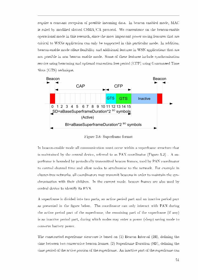
require a constant reception of possible incoming data. In beacon enabled mode, MAC
is ruled by modi�ed slotted CSMA/CA protocol. We concentrate on the beacon-enable
operational mode in this research, since the most important power saving features that are
critical to WSNs application can only be supported in this particular mode. In addition,
beacon-enable mode o�ers �exibility and additional features in WSN applications that are
not possible in non beacon enable mode. Some of these features include synchronisation
service using beaconing and optional contention free period (CFP) using Guaranteed Time
Slots (GTS) technique.
Figure 2.8: Superframe format
In beacon-enable mode all communication must occur within a superframe structure that
is maintained by the central device, referred to as PAN coordinator (Figure 5.2) . A su-
perframe is bounded by periodically transmitted beacon frames, used by PAN coordinator
to control channel time and allow nodes to synchronise to the network. For example in
cluster-tree networks, all coordinators may transmit beacons in order to maintain the syn-
chronisation with their children. In the current mode, beacon frames are also used by
central device to identify its PAN.
A superframe is divided into two parts, an active period part and an inactive period part
as presented in the �gure below. The coordinator can only interact with PAN during
the active period part of the superframe, the remaining part of the superframe (if any)
is an inactive period part, during which nodes may enter a power (sleep) saving mode to
conserve battery power.
The constructed superframe structure is based on (1) Beacon Interval (BI), de�ning the
time between two consecutive beacon frames, (2) Superframe Duration (SD), de�ning the
time period of the active portion of the superframe. An inactive part of the superframe can
51

only be de�ned when BI is greater than SD. BI and SD are determined by two MAC PAN
information base parameters, the macBeaconOrder, BO, describes the interval at which
the coordinator transmits its beacon frame and macSuperframeOrder, SO, describes the
length of the active portion of the superframe respectively. The value of BO and SO are
related to beacon interval, BI, and superframe duration, SD, respectively, as follows:
For 0=<BO=<14, BI = aBaseSuperframeDuration * 2^BO symbols
The values of SO related to the superframe duration, SD, are related as follows: for
0=<SO=<BO=<14, SD = aBaseSuperframeDuration*2^SO symbols The active portion
of each superframe is divided into aNumSuperframeSlots equal spaced of duration 2^SO
* aBaseSlotDuration and aBaseSuperframeDuration = aBaseSlotDuration x aNumSuper-
frameSlots. Assuming 250kbps in 2.45 GHz frequency band, aBaseSlotDuration equals
to 60 radio symbols resulting 15.36ms minimum SD(SO = 0) with 16 superframe slots.
Hence (BI) and SD may be between 15.36ms and 251.7s. In case of non beacon-enable,
both macBeaconOrder and macSuperframeOrder are set to 15 by PAN coordinator and
therefore an unslotted CSMA-CA mechanism is used to access the channel.
In beacon-enable mode, the 16 contiguous time slots in the active period part of each
superframe are composed of three parts: the beacon, contention access period (CAP)
and contention-Free period (CFP). The beacon transmitted without the use of CSMA, at
the start of slot 0, followed by CAP and CFP to the end of active part of superframe. In
addition to the beacon, CAP is mandatory part of a superframe. Coordinators are required
to listen to the channel the whole CAP to detect and receive any data from their child
nodes. On the other hand, the child node may only transmit data and receive an optional
acknowledgement (ACK) when needed, which increases their energy e�ciency.
Downlink data from a coordinator to its child require a total four transmissions. The
availability of pending data is signaled in beacons. First, a child requests the pending data
by transmitting a data request message. The coordinator responds to the request with
the ACK frame, and then transmits the requested data frame. Finally, the child transmits
ACK if the data frame was successfully received.
All frames, except acknowledgement frames and any data frame that quickly follows the
acknowledgement of the data request command, transmitted in the CAP will use a slotted
CSMA-CA mechanism to access the channel. A device transmitting within CAP shall en-
sure that the transaction is complete (i.e including the reception of any acknowledgement)
52

one IFS period before the end of the following superframe. If this is not possible, the device
shall defer its transmission until the CAP of the following superframe.
2.13.1 The CSMA-CA procedure
The CSMA/CA procedure is used for each data frame transmission or MAC command
frame during contention access period (CAP). The CSMA/CA will not used during the
transmission of beacon frames, acknowledgement frames or data frames transmitted during
contention free access (CFA) and any data frame that quickly follows the acknowledgement
of data request command . In beacon enable mode, the MAC sublayer uses the slotted
version of the CSMA/CA algorithm for transmission in the CAP of the superframe. If
beacons are not used then unslotted version of CSMA/CA algorithm is used. In slotted
CSMA/CA, the backo� period boundaries of every device in the PAN shall be aligned
with the superframe slot boundaries of the PAN coordinator. i.e. the start of the �rst
backo� period of each device is aligned with the start of the beacon transmission. In
slotted CSMA/CA, the MAC sublayer shall ensure that the PHY commences all of its
transmissions on the boundary of a backo� period. In the case of unslotted CSMA/CA,
the backo� periods of one device are not related in time to the backo� periods of any other
device in the PAN.
The CSMA/CA mechanism is based on a basic time unit referred to as Backo� Period (BP),
which is equal to aUnitBacko�Period = 80 bits or 20 symbols, i.e. 0.32ms in 2.45 GHz
frequency band. The slotted CSMA/CA can be summarized in �ve steps. To accessing
the channel or each transmission attempt, each node maintains three variables: 1) NB is
the number of backo� attempts for the current transmission, initialized to 0 before each
new transmission attempt. 2) BE is the backo� exponent, which de�ne the number of
backo� periods a node should wait before attempting to assess the channel or perform a
clear channel Assessment. With macBattLifeExt set to FALSE, BE shall be initialized to
the value of macMinBE. In slotted systems with macBattLifeExt set to TRUE, this value
shall be initialized to the lesser of 2 and the value of macMinBE. 3)CW is the contention
window length, which de�ne the number of consecutive backo� periods a channel needs
to be silent before transmission can commerce (Default value = 2) CW=2 before each
transmission attempt and reset to 2 each time the channel is accessed to be busy. The CW
variable is only used for slotted CSMA/CA. The backo� period length (tBOP) is de�ned
as 0.32ms in the 2.4GHz band.
53

When using slotted CSMA/CA First, the MAC sublayer initializes NB, CW, and BE, and
then locates the boundary of the next backo� period.
Second, The MAC sublayer delay for a random number of complete backo� periods in the
range 0 to 2^BE � 1
Third, MAC request that the PHY perform a CCA, in slotted CSMA/CA, the CCA shall
start on the backo� period boundary. In unslotted, the backo� starts immediately.
Fourth, if channel is assessed to be busy, the MAC sublayer shall increment both NB and
BE by one, ensuring BE shall not be more than the aMaxBE. MAC in slotted shall also
reset CW to 2. CSMA/CA will return to step two if the value of NB is less than or equal
to macCSMABacko�s. CSMA-CA will terminate with a Channel Access Failure status if
the value of NB is greater than macCSMABacko�s.
Fifth, if the channel is accessed to be idle, the MAC sublayer in slotted CSMA/CA system
will ensure that the contention window has expired before commencing transmission. To do
this CW is decremented by 1 and if it reaches zero then the data is transmitted otherwise
the algorithm goes back to step 3. This ensures that CCA is performed twice to prevent
potential collisions of acknowledgement frames. If the channel is again sensed to be idle,
the node attempts to transmit provided that the remaining BPs in the current CAP is
su�cient to complete the transaction (i.e including the reception of any acknowledgement)
one IFS period before the end of the following superframe. If this is not possible, the
device shall defer both CCAs and frame transmission until the next CAP of the following
superframe.
2.13.2 The Self-Organisation and Self-Con�guration Aspect
One of the very important aspects of wireless sensor networks is that of an ad-hoc prop-
erty whereby wireless networks should exhibit self-organising and maintaining of the net-
work. The major activities that an ad-hoc network is required to perform to achieve
self-organisation are neighbour discovery, topology organisation and topology reorganisa-
tion. During the neighbour discovery phase, every node in the network gathers information
about its neighbors and maintains that information in appropriate data structures. This
information is obtained periodically either by sending short packets called beacons, or by
promiscuous snooping on the channel to detect any neighbours' activities.
54
2.14 Conclusions
The literature review focused on a range of WSN research and development in both phys-
ical layer and medium access control (MAC) sublayers, the IEEE 802.15.4 standard, and
key concepts and theories relating to this research. The literature review included a re-
view on the transmission power control, IEEE 802.15.4 medium access control (MAC),
and self-con�guration. The IEEE 802.15.4 is designed for low rate wireless personal area
networks (LR-WPANs), making it the �rst WSN-enabling standard. However, the devel-
opment of a particular WSN application will require solutions, integrated to a high degree,
for both robust hardware and e�cient protocols or software to achieve e�ective communi-
cation. So far there have been no clear guidelines or design rules that had to be followed
in designing sensor network architectures because of the wide range of sensor applications,
with each application having its own unique purpose and performance requirements (i.e.,
various hardware and network capabilities). Furthermore, both the general WSN archi-
tecture and hardware architecture for WSNs with a detailed comparison of some of the
currently available hardware components were presented. The object of such a comparison
is to provide information about some of the latest innovations, and the challenges to face
and solutions to consider when developing new ones. These forefront initiatives require
a balance between power consumption and other performance parameters. The optimal
choice of sensor system, processor, wireless interface, and memory technology is not only
application dependent, but also exhibits temporal dependence for a given application.
55

56

Chapter 3
Problem Formulation and Background
3.1 Introduction
In Chapter 1, the purpose of this study was de�ned �to investigate strategies to improve
the performance of WSNs to maintain reliable network connectivity, improve scalability
and save energy�. Having established the background literature framing in Chapter 2, this
Chapter directs the emphasis on the research questions and the approach used to address
them or the research methodology.
The structure of the chapter can be summarised as follows. Section 3.2 of this chapter
provides an overview of the background and motivation for this research. Section 3.3
includes a detailed presentation to research questions, background and the approach used
to address the questions. Section 3.4 presents a summary of research contributions. Section
3.5 describes the methods and tools used in this research, and Section 3.6 describes some
of the essential performance parameters in this study. Section 3.7 presents the general
research assumptions and Section 3.8 discusses some of the research limitations and future
research directions. Section 3.9 concludes the chapter.
3.2 Background to the Research
Traditionally, sensor networks have been connected via considerably reliable wired net-
works. However, establishment and maintenance costs for these networks comprise 33~70%
of the entire system cost [1, 2, 3, 4]. The advantages of wireless connectivity include the
57
likelihood of saving the network's establishment and running costs . In the near future,
sensor networks will be able to support new opportunities or applications for interaction
between humans and their physical world. Speci�cally WSNs are expected to contribute
signi�cantly to pervasive computing and space exploration. Deploying sensor nodes in an
unattended environment will provide tremendous possibilities for the exploration of new
applications in the real world. However, this area of study is still underdeveloped. Fur-
thermore, the lack of relevant guidance and practical approach when dealing with WSN
applications means that solutions are needed.
The main motivation behind this research study is a belief that the performance of WSNs
may bene�t from further cross-layer protocol improvements and further knowledge regard-
ing the operation of a particular protocol. The initial research cycle identi�ed general
problems in wireless sensor networks. Thus investigation of how performance of WSNs
could be improved and how this could be better integrated into the working IEEE 802.15.4
standard was required. While a wide-range of research in wireless networks thrives on ways
to improve the quality of service (QoS) of wireless networks for multimedia applications.
The primary performance objectives of wireless sensor networks in most cases are energy
conservation, throughput improvement, scalability and self-con�guration, whereas fairness
and temporal delay are often secondary issues [20].
We anticipate that to achieve technological and marketplace success, the low power, in-
expensive sensor networks need to achieve energy e�ciency and reliable connectivity. En-
hancing communication networks for reliable wireless connectivity, self-con�guration, cost
e�ectiveness and energy e�ciency is the challenge for WSNs. For example, ability to work
with minimum energy consumption will prolong the network lifetime. Since sensor nodes
share a common wireless medium, an e�cient medium access control (MAC) operation is
required; however other issues which cannot be ignored include topology changes or mo-
bility, multi-hop communication, self-con�guration, unattended nature of wireless sensors
(power), connectivity, and throughput improvement. In particular, a WSN application will
require a high level of system integration, performance, and productivity.
3.3 Research Main Objective and Questions
The main purpose of this research is to investigate means to improve the performance
of WSNs to maintain reliable network connectivity, scalability and energy e�ciency. The
58
study focuses on the IEEE 802.15.4 MAC/PHY layers and the carrier sense multiple access
with collision avoidance (CSMA/CA) based networks. So the main research question is
�how and what can be done to improve the performance of WSNs to maintain reliable net-
work connectivity, scalability and energy e�ciency in the IEEE 802.15.4 based networks?�
To answer this question, this research consists of four semi-independent areas of study
and therefore four backgrounds to the problem. The following subsections present the
four main research areas of the study and questions that this research set out to explore.
For the purpose of clarity, each of these four areas of study including results is addressed
separately in Chapter 4, Chapter 5, Chapter 6 and Chapter 7 of this thesis (see Table of
Contents).
3.3.1 The impact of multi-hop and transmission power control in 802.15.4
This �rst major theme connects directly to the discussion in the literature review that an N
hop multi-hop communication can be more energy-e�cient than single-hop communication
for same distance, Nr by deriving the following expression:
ηrf =Psend (Nr)
N.Psend (r)=
(Nr)α PreceivedN.rαPreceived
= Nα−1
where r , α, Psend, and Preceived are the one-hop distance, radio frequency (RF) attenuation,
the power at a transmission node, and the minimum received power at a node respectively.
We take the relationship between the number of hops and transmission power control, and
pay particular attention to the likelihood that multi-hop might be bene�cial for energy
saving in WSNs. In consideration of these points and the speci�c literature review in
Chapter 4, the basic research questions which are addressed in Chapter 4 are:
1. How can we speci�cally test multi-hop TPC communication versus single-hop com-
munication using typical wireless sensor node hardware parameters?
2. What is the performance advantage of using multi-hop TPC in energy constraint
WSNs instead of a single-hop in terms of energy e�ciency and other important per-
formance parameters? Essentially, I what to determine as to whether transmission
power control in multi-hop communication is more energy superior than single hop
59

communication and by how much with an increasing number of hops. Further ques-
tions concerning multi-hop TPC grow out of these, for instance, are there any ways
that we can use TPC to improve energy e�ciency in WSNs ?
3.3.2 The impact of beacon interval in association and synchronization
This second major theme is the self-con�guration aspect of WSNs, which also connects
directly to the discussion in the literature review in Section 2.13. One of the key aspects of
a wireless sensor network is its ability to self-organize and maintain connectivity. Medium
Access Control (MAC) protocol manages network self-con�guration, which includes es-
tablishing a personal area network (PAN), �nding a network to associate or disassociate
with, and synchronizing if required. In beacon-enable mode all communication must occur
within a superframe structure that is maintained by the central device, referred to as PAN
coordinator. A superframe is bounded by periodically transmitted beacon frames, used by
PAN coordinator to control channel time and allow nodes to synchronise to the network.
Currently, there is limited research addressing the network initialization phase or self-
con�guration phase. This appears to be the �rst investigation of the performance of the
802.15.4 MAC beacon interval setting and the number of associating nodes. The perfor-
mance evaluation is based on the number of nodes associating with a coordinator and
beacon intervals in terms of the time required for a node to associate with its coordinator
(association delay) and energy consumed by a node to associate and synchronize with the
coordinator. In consideration of these points and the speci�c literature review in Chapter
5, the basic research questions addressed in Chapter 5 are:
3. What is the impact of beacon interval (BI) and number of nodes during WSN associa-
tion and synchronization stages in terms of energy and association or synchronization
time?
4. How can we improve the performance of WSNs during association and synchroniza-
tion stage (self-con�guration)?
3.3.3 Clear channel assessment and enhanced MAC
This third major theme connects directly to the discussion in the literature review on the
IEEE 802.15.4 MAC protocol standard controlling radio channel access using the Carrier
60

Sense Multiple Access with Collision Avoidance (CSMA/CA) algorithm. To avoid col-
lisions, the standard adjusts the backo� exponent (BE) based on two consecutive clear
channel assessments (CCA) before packet transmission. The CCA part is carried out at
the physical (PHY) layer, and used by the MAC protocol as part of the CSMA/CA al-
gorithm, whereby a node is required to perform a CCA for a predetermined duration to
determine if the channel is available for transmission before transmission of the data frame.
In consideration of these points and the speci�c literature review in Chapter 6, the basic
research questions addressed in Chapter 6 are:
5. What is the impact of the number of times the clear channel assessment (CCA) is
performed in the 802.15.4 MAC during frame transmission in terms of throughput,
packet error rate, delay and energy consumption for both hidden and non-hidden
nodes in a network ?
6. What can be done to improve the performance of the 802.15.4 MAC during frame
transmission stage?
3.3.4 Analysis of CSMA/CA using Markov chain
The last major theme, similar to the previous section connects directly to the discus-
sion in the literature review on the IEEE 802.15.4 MAC protocol standard that controls
radio channel access using the Carrier Sense Multiple Access with Collision Avoidance (CS-
MA/CA) algorithm. However, Markov Chain theorems were used to model the CSMA/CA
operation in order to be able to forecast the performance outcome for CSMA/CA. This
is of prime importance to protocol designers since one can use the insight gained using
Markov Chain to �ne-tune ones design strategies. Obviously in analytical mathematical
modelling, one relies on assumptions and approximations made to simplify mathematical
expressions while closely modelling/describing an original protocol or process.
Considering these points and the speci�c literature review in Chapter 7, the basic research
questions addressed in Chapter 7 are:
7. How can Markov chains be used to accurately model the IEEE 802.15.4 slotted
CSMA/CA ?
8. What is the relationship between di�erent performance variables and the MAC pa-
rameters derived from the Markov Chains?
61

3.4 Signi�cance of the Study
This section provides a brief description on various signi�cances of the study. This research
is bene�cial to students, researchers and network designers as it contributes further knowl-
edge to the WSN area of research particularly on network connectivity, scalability, energy
e�ciency, self-con�guration and possible MAC and physical layer cross layer enhancements.
The research serves future researchers baseline information on the recent advancement of
WSNs and their possible performance improvements. This research provides a practical
outcome to assist network engineers or designers in developing and improving more e�ec-
tive protocols for WSNs. Several works relating to this thesis have been published during
the course of candidature. The list of publications can be found on pages xi-xii of the
thesis.
The main contributions of this research have been described in Chapter 1 and also reviewed
in the �nal chapter. The signi�cance of the research relates to the outcomes of the four
semi-independent areas of study described in Section 3.3 above.
In summary, the main research contributions listed according to the research question
number (Section 3.3) are:
1. This study has developed a novel approach to testing multi-hop and single-hop trans-
mission power control (TPC) at the physical layer using typical wireless sensor node
hardware parameters.
2. One of the more signi�cant �ndings to emerge from this study is the evidence that
contrary to what has been reported from previous studies, in multi-hop networks,
TPC did not save energy. Both the radiation and electronic components of the energy
consumption were investigated, and results indicated that sending packets using a
short-range multi-hop path, instead of a single-hop, does not necessarily save energy
as suggested by some researchers. The results of this study support the idea that a
better topology such as cluster topology is required rather than �at topology
3. The study has added to the body of knowledge as it appears to be the �rst inves-
tigation of the performance of the 802.15.4 MAC beacon interval setting and the
number of associating nodes. The study �ndings suggest that over a longer period,
shorter beacon intervals will consume more of the node's energy while long beacon
62

intervals will spend less energy, at least for BO=0 to BO=11. The associating en-
ergy consumption increases with increased number of nodes for all beacon intervals
(B0=0-15). For longer beacon intervals, BO=12 to BO=14, there is an abrupt in-
crease in energy consumption as the number of associating nodes increases, even
for a small number of nodes, such as four. This study has shown that it will take
about 42 minutes for 7 nodes requesting association to associate with the coordina-
tor, when BO=14. Such long delays are not suitable for real time and mobile WSN
applications.
4. The �ndings of this study raised a question as to whether the association energy
consumption will outweigh the bene�t of duty cycle power management for larger
beacon intervals, as the number of associating nodes increases. The evidence from
this study suggests a need for a better protocol design to resolve this.
5. The most obvious �nding to emerge from this study is that there is serious network
performance degradation even for a small number of hidden nodes in a network.
The results of this study also indicate that there is some improvement in terms of:
1) throughput; and 2) average packet delay, when sensing the channel for shorter
duration (once), instead of twice or thrice as the tra�c load increases; however
there is no signi�cant di�erence in energy consumption and packet error rate. An
implication of this is the possibility that that likelihood of a channel being idle or
busy the second or third time is smaller once it has been sensed busy or idle the �rst
time.
6. The study provides a proposed cross layer (PHY-MAC) mechanism to save energy,
reduce interference, improve scalability and reliability, and reduce packet collisions
due to hidden terminals.
7. The study developed an analytical model for the IEEE 802.15.4 slotted CSMA/CA
scheme using Markov chains. The body of knowledge was increased by the de-
velopment of theoretical understanding related to IEEE 802.15.4 operational and
performance of CSMA/CA.
8. The study developed model captures essential features of the slotted CSMA/CA
that can be used to forecast some of the performance parameters such as successful
transmission probability, throughput and average energy consumption.
63

3.5 Research Methods and Tools
The design and investigation in the current research has been carried out using a com-
bination of simulation, numerical method and Markov chain modelling. To answer the
research question posed above di�erent methods were used given that the research consists
of four semi-independent areas of study as described in Section 3.3 above. The methods
and �ndings for each study area are covered in Chapter 4, 5, 6 and 7 respectively. The ob-
jectives and research questions elaborated in the previous section will mainly be addressed
via NS 2 simulations, which is the main research instrument for this thesis. Where possible
theoretical mathematical numerical and analysis will be provided.
The research methods involved investigation, analysis and proposed improvements in the
MAC and Physical layer, particularly in the IEEE 802.15.4 based WSNs. Both strengths
and weaknesses of the protocols are determined. Experiments, implementations and re-
search questions were addressed using NS 2 simulations and where possible numerical
mathematical expressions and analytical modelling was carried out using Markov Chain
theorem. NS 2 is the main methodological approach used in this research. We use NS 2
for implementation, modelling and simulation of a real system to help us answer research
questions.
There are numerous software tools used in our research. Some of these software tools
include Eclipse, which was used to develop and debug our C++ implementation code [85].
Doxygen [86] was used extensively for documentation of existing protocol implementation
in ns-2 and our implementation. We provide an overview description of ns-2, which is the
main simulation and protocol implementation design tool used throughout the research.
Furthermore, we provide the steps involved in implementing and simulating a particular
network scenario using ns-2 simulator and discuss some of the ns-2 limitations.
3.5.1 Network Simulator 2 (NS 2)
NS-2 is one of the most widely used publicly available object oriented, discrete event driven
network simulators used in education and research today. The ns simulator project was
started as a variant of the REAL network simulator in 1989 and evolved substantially ever
since. The simulator is written in C++ and it uses OTcl interpreter as a command and
con�guration front-end. It supports a large number of packet switching protocols and also
64

provides a very rich �exible platform for developing and testing new protocols. Using ns-2
�exibility, one can simulate variants of available network protocols or design a new protocol
using available �exible models.
NS-2 is capable of simulating mobile nodes connected by wireless interfaces using 802.15.4
standard protocol. In the current research thesis, ns-2 with the wireless extension imple-
mented by the Rice monarch Project was used [82]. Given all these features, i.e. open
source, �exibility and great design potential, ns-2 was chosen as the developing and testing
platform in the current research.
In this we describe some of the tools and methods used in the current research for the
investigation and protocol design using a Network Simulator (NS-2) [82]. It focuses on
development of a framework for designing, optimising, analysing and carrying out perfor-
mance measurement of 802.15.4 standard and proposed design for wireless sensor networks.
Supplementary information about the simulator can be found in an Appendix A, which
includes the following sections: Installation and Settings, Simulator Internal Architecture,
The Concept of Discrete Event Driven, Ns-2 Simulation, Extending New Implementation/-
Coding, Extracting Information from the Trace Files, and Simulation Visualization.
3.5.2 Research Framework/Simulation Environment
The summary of overall simulation environment is shown in Figure 3.1. The text editor
is used for writing awk scripts and OTcl script to setup the network, tra�c and other
simulation parameters. Variable speci�cation and implementation changes can be done
solely using OTcl or by changing the C++ network elements code. Upon running tcl
script in ns-2, ns-2 will generate trace �les that contain events record (trace�le) and for
NAM (NAM trace �le). These �les are then processed for further analysis. Note that
in the Figure 3.1, gnuplot, Eclipse, awk or perl script and doxygen are not part of the
ns-2 simulator. These tools are used for further processing of information produced by the
ns-2 simulator. For example, doxygen was used to produce documentation for the NS 2
C++ code. Awk scripts are used to extract relevant information and obtain a particular
performance parameter of interest from the large trace �le. The relevant information
obtained can then be analysed and plotted using one of the graphics tools.
65

Figure 3.1: Research framework
3.5.3 Markov Chain Analysis
A discrete Markov chain model was used in the last study area as a methodological ap-
proach to answer the research questions. Generally, a discrete Markov process {Xn} is a
stochastic process with the property that the probability of any particular future behaviour
of the process, when the current state is known exactly, is not altered by additional knowl-
edge concerning its past behaviour. From the de�nition {Xn} is Markov chain if
Pr {Xn+1 = j | X0 = io, ....Xn−1 = in−1, Xn = i} = Pr {Xn+1 | X = i}
For all time points n and all states i0.......in−1, i, j.
Notation : Pr {Xn+1 = j | Xn = i} = Pij , where
Pij ≥ 0 for i, j= 0,1,2.... and∑∞
j=0 Pij = 1 for i = 0, 1, 2, 3, ...
Once all the transition probabilities have been obtained, the Markov chain can be numer-
ically solved to obtain the stationary probability distribution of each state using recursive
solution, π = πA, where A is the initial state condition and πis the transition matrix.
66
3.6 Performance Metrics and Analysis
Performance measurements are carried using results obtained from ns-2 simulations and
where possible, analytical and numerical models were used in the analysis of our �ndings.
3.6.1 Throughput
Network performance is a measure of a network's performance throughput, which is the
amount of data transferred from one place on the network to another or the amount of
data processed over a speci�ed amount of time. Data transfer rates for network are mea-
sured in terms of throughput. In general, throughput is measured in kilobits per second
(Kbps), megabits per second (Mbps) and gigabits per second (Gbps). Apart from mea-
suring the bandwidth of a network, network performance also takes into account how
fast a piece of data travels from one part of a network to another. Furthermore, net-
work performance takes into account dropped (lost) network packets. The throughput
thus equals the o�ered load multiplied by the probability of successful packet reception,
throughput = load ∗ probability, where this probability is a function of the random access
protocol in use as well as the channel characteristics, which can cause packet error in ab-
sence of collisions. Performance of random access techniques is typically characterized by
the throughput of the system. A high performance network, has therefore, high bandwidth,
quick transfer rates, and low rates of packet loss. The achieved throughput in an ad-hoc
network is a�ected by numerous factors that include radio interference between hops, abil-
ity of the routing protocol to react to topology changes and a complex interaction between
the application and underlying protocols. Furthermore, UDP and TCP performance is
reduced in a multi-hop 802.15.4 WPAN environment because of radio interference between
hops.
Throughput is the rate at which network sends or receives data and a good measure of
channel capacity.
The aggregate throughput, S in a simulation study can be obtained by using the following
expression:
S =TotalReceivedBytes× 8
Simulation T ime×Bit Rate(3.1)
67

3.6.2 Packet delivery ratio or Bit Error Rate
This performance metric presents the ratio of total data packets successfully received or de-
livered to the destinations application layer to total packets generated or sent by sources.
It is desirable to have a high packet delivery ratio for e�cient bandwidth utilization in
wireless networks where available bandwidth is a limiting factor. This performance mea-
surement is important because it reveals the loss rate seen by transport protocols and also
characterises the completeness and correctness of the MAC and routing protocols. There
are number of factors that can cause high BER, such as signal interference caused by de-
vices in the same frequency spectrum, multipath fading, packet collision, the quality of
the channel and established links. For wireless sensor networks, a BER of less than 10-5
is acceptable. Delivery ratio in a simulation study can be obtained by using the following
expression:
Delivery ratio =Number of delivered packets
Total number of transmitted packets(3.2)
3.6.3 End-to-end delay
End-to-end delay of data packets is another important metric of performance that involves
sources and receivers. The end-to-end delay is the total delay that a data packet experiences
as it is traveling through the network from the sources through wireless media to the
destination. This delay is built up by several smaller delays in the network that add
together. These delays include bu�ering delay during route discovery latency, the time
spent queuing at the interface queue, forwarding delays, propagation delay and the time
needed to make retransmissions in the case of packet lost.
End-to-end delay in a simulation study can be obtained by using the following expression:
Delay = Packet destination arrival time− Packet source send time (3.3)
3.6.4 Energy E�ciency
A sensor network is expected to have a long operational life to further reduce the cost
of maintenance and deployment. Energy e�ciency (normalised energy) is often the key
68

performance parameter in most WSN applications due to limited battery life. We de�ne
energy e�ciency or the e�ective transmission energy per packet as the ratio of total amount
of data delivered and total energy consumed or by determining the total transmission
energy spent in transferring an amount of tra�c load, e.g. 20 byte, from a source node
to a destination node. Similarly, the energy per bit is de�ned as the energy consumed by
the network to successfully deliver a bit of data to the sink averaged over all nodes. It is
desirable to have energy e�cient hardware and protocols to improve energy e�ciency and
prolong the life time of wireless sensor networks.
Energy e�ciency in simulation study can be obtained by using the following expression:
E =Total amount of data delivered
Total amount of energy consumed(3.4)
3.7 General Research Assumptions
The general assumptions made in the following research include:
� No multipath fading: Multipath fading is when we consider Radio Frequency (RF)
signals travelling in all directions, which results into multipath fading and therefore
may a�ect wireless communication. Because of complexity and di�culty of simulat-
ing and modelling multipath fading. In this research, Freespace and Two-ray ground
propagation models were used to provide easy modelling and simulation while provid-
ing signi�cant accuracy. However, the issue of multipath fading is a good candidate
for future work.
� Homogenous network: the investigations and design development in this research
considered homogeneous sensor networks, i.e. it is assumed that all nodes in the
sensor network have the same capability. However, there are important WSN ap-
plications where this is not the case. Future studies should include heterogeneous
sensor networks that consist of several nodes with extra capability in a network.
� No interference: Most of WPANs or WSNs communications use the Industrial, Sci-
enti�c and Medical (ISM) frequency band. This frequency band is unlicensed and
it is widely used by many other electronic devices. Since it is not easy to control
69

interference from other devices, we assumed that there is no interference due to de-
vices that operate in the same frequency band. Future studies should include other
conditions that wireless channels are likely to encounter, such as noise, interference,
and other environmental factors, such as temperature, humidity, and wind.
Since there are four areas of study, several other research assumptions unique to those
study areas are addressed in the succeeding Chapters 4, 5, 6 and 7 respectively.
3.8 Research Limitations and Implications for Further Re-
search
Apart from the research limitations drawn from the assumptions made in the section above.
Our �ndings in this research are subjected to at least two limitations. First, obviously the
time period of my candidature where this research was conducted. Secondly, is the fact
that the current investigation was conducted using a simulator and mathematical theories
and not a hardware platform. However, the research has been conducted careful to closely
re�ect the hardware systems.
Further investigation and experimentation using suitable hardware platforms in the exper-
imentation and implementation phases of the current and future work is recommended.
The following sections provide important insights for those interested in using hardware
investigation and experimentation in the current area of research.
3.8.1 Challenges of implementing MAC in embedded systems
Embedded system applications are highly integrated and constrained to minimize cost
among other factors. Currently, most of the MAC protocols are running on the main
processor. Many challenges exist when porting or implementing a new MAC protocol in a
particular platform including the variety of existing operating systems (OS) with variety
services and system software interface for MAC, the diversity in radio transceiver interfaces
and features, the diversity of instruction set architecture features and compiler support,
and the degree of �exibility and network performance inherent tradeo�.
The MAC protocol implementation to a greater extent depends on the radio transceiver
and microprocessor or processor in use. The number of available hardware features for
70

transceivers, microprocessors and interfaces require di�erent MAC instruction set for MAC
implementation and compiler support. From a view point of the OS and a portable MAC
implementation, the primary di�erences are the interfaces to time facilities, memory man-
agement, interrupt handling, interprocessing communication and hardware peripheral ac-
cess. Most of IEEE 802.15.4 MAC implementation are targeted at microcontrollers allowing
nesting prioritization of interrupts. For example freescale provides such an IEEE 802.15.4
MAC implementation, which is independent of operation system [87]. TI also provides
an interrupt based implementation of 802.15.4 MAC for its CC2420 transceiver. When
migrating these implementation to hardware platforms with limited interrupt handling
capabilities, rewriting of possibly a large portion of the code will be necessary.
Another challenge is on cross-layer coupling of functions, since there is a strict interde-
pendence among functions handled at all layers of communication protocol stack. This
has to be explicitly considered when designing communication protocols aimed at QoS
provisioning on resource constrained.
3.8.1.1 Designing, debugging and Programming tools
Most of the popular hardware vendors provide their own IDE for developing and debugging
their systems. One example is the Atmel AVR, which o�ers several options for debugging,
mostly involving on-chip debugging while the chip is in the target system. AVR Studio® 5
makes editing and debugging source code easier by seamlessly bringing together an editor
with assisted code writing, a wizard for quickly creating new projects, an AVR software
framework source code library, a GNU C or C++ compiler, a powerful simulator, and
a front-end visualizer for all of Atmel's AVR programmers and in-circuit debuggers [52].
AVR Studio 5 combines the best features of the current 8-bit AVR Studio 4 and 32-bit
AVR32 Studio into one environment that covers all 8- and 32-bit AVR MCUs. It also
gives the user easy access to online documentation including device data sheets, tools user
guides, example project documentation, and kit shopping directly from the Atmel online
store. Atmel's AVR Studio 5 further provides an integrated o�ering of third party plug-ins
for embedded development tools.
A common debugging interface is JTAG (Joint Test Action Group), which is often used
in Microcontrollers [88]. JTAG provides access to on-chip debugging functionality while
the chip is running in the target system. JTAG allows accessing internal memory and
71

registers, setting breakpoints on code, and single-stepping execution to observe system
behavior. Atmel provides a series of JTAG adapters to program AVR chips, however the
methods to program AVR chips varies from AVR family to family. Other ways include
the In-system programming (ISP) programming method, which is functionally performed
through SPI, plus some twiddling of the Reset line, debugWIRETM is Atmel's solution
for providing on-chip debug capabilities via a single microcontroller pin. It is particularly
useful for lower pin count parts which cannot provide the four "spare" pins needed for
JTAG.
3.9 Conclusion
In this chapter, a research methodological framework layout is presented. The research
is concerned with developing and evaluating techniques for improving the performance of
WSNs to maintain reliable network connectivity, scalability and energy e�ciency. The
research questions were presented under four areas of study, and their justi�cation or eval-
uation phase and results was linked to the four areas of study in the succeeding Chapters 4,
5, 6 and 7. The evaluation process was brie�y described which involved simulation studies,
numerical and mathematical analytical modelling. Lastly, the main research contributions,
performance parameters, research assumptions, limitations and future methodological re-
search were addressed.
72
Chapter 4
Transmission Power Control for Sensor Networks
Because of the need to minimise energy consumption of sensor nodes to pro-
long battery life in sensor network. Power control has been one of the main
techniques used to conserve energy in wireless sensor networks, particularly in
star topology or cellular networks. This chapter provides a conclusively demon-
stration of some relevant advantages of single-hop transmission power control
(TPC) over multi-hop. TPC is investigated in multi-hop and single-hop WSNs
using typical Telosb platform parameters, which are IEEE 802.15.4 standard
compliant. A new detailed approach is also presented for testing TPC for
multi-hop and single-hop WSNs at the physical layer. Following this approach,
energy consumption performance results via simulation and a numerical analy-
sis are presented, and results indicate that sending packets using a short-range
multi-hop path, instead of a single-hop, does not necessarily save energy as
suggested by some researchers [31, 32, 33]. Moreover, transmitting in single-
hop networks at lower transmission power levels, while still maintaining reliable
connectivity, reduced energy consumption by up to 23%. Both the radiation
and electronic components of the energy consumption are characterised. Fur-
thermore, the research shows that both packet collisions and delays a�ect the
performance of WSNs that have an increased number of hops. Since the use of
TPC in star topology or cellular networks transmission can save energy, we rec-
ommend cluster based (hybrid) or similar topology over completely multi-hop
topology. The relationships among protocol layers are also revealed, possible
improvement suggested, insights are provided into challenges associated with
developing wireless sensor networks protocols and the signi�cance of TPC is
highlighted;
73

4.1 Introduction
A major challenge in sensor network protocol design is minimizing energy consumption by
nodes to prolong network endurance, while still maintaining e�ective communication. We
expect the emerging WSNs to be more energy-e�cient, given that the compactness and
increasing density of new wireless devices impose greater constraints on battery capacities.
There are several techniques for minimizing energy consumption in a WSN, which can be
categorized into: e�cient data aggregation, e�cient routing, MAC layer power manage-
ment, and topology management using transmission power control. This chapter focuses
on TPC, which is one of the promising and e�ective techniques for minimizing interference
and reducing sensor node energy consumption. TPC allows a transmitter to dynamically
change the transmission output power to the minimum level, depending on the receiver
proximity, and still maintain a reliable link. TPC has been widely studied in the liter-
ature, particularly in cellular networks and IEEE 802.11 networks. Our work, based on
the 802.15.4 physical layer, relies on all sensor nodes having adjustable transmission power
levels. While researchers have addressed cellular TPC algorithms in cellular networks, no
comprehensive published work was identi�ed which compares energy e�ciency in multi-
hop communication over equal distances from source to sink. Although some researchers
suggest that short-range multi-hop communication is more energy-e�cient [31, 32, 33], our
simulation and numerical results do not support this conclusion.
Earlier studies have sought to improve WSN performance (such as throughput, and power
consumption) by varying transmission power. In[74, 89, 90], Power control in 802.11 stan-
dard was used to increase the channel e�ciency rather than prolong battery life. Their
work is based on RTS/CTS protocols and considered the issues of exposed and hidden
terminals in networks. While 802.11 is power-hungry and therefore unsuitable for WSN
applications, these studies can be extrapolated and used for WSN protocol design.
In [91, 92], transmission range adjustment was adopted to avoid overlapped sensing area
while still maintaining e�ective coverage. The objective was to minimize energy consumed
by the sensing function rather than during communication. In this chapter, we energy
consumed to transmit information from source to destination is addressed.
Zhao [31] suggests that multi-hop communication can be more energy-e�cient than single-
hop communication. He derives an expression to show the power advantage of a N-hop
74
transmission over a single-hop transmission over the same distance. This simpli�ed model
favors the multi-hop scenario. Monks [33] and Kai [32], also suggest that information from
a source should go through one or more intermediate hops to reach its destination in order
to achieve desired power savings.
Various models have been used to address transmission power, Bandai [93] using a Friis
transmission equation, suggesting that a shorter distance hop greatly decreases transmis-
sion power, while Liu [81] considered a variable Physical carrier sense (PCS), based on
background noise to minimize collision and therefore minimize energy consumption.
Our derived energy model is based on research by Heinzehman [94]. We address transmis-
sion power control at the lowest general PHY layer and therefore our �ndings can be used
in the implementation of MAC or the network layer. We consider commercially available
low-energy sensor nodes (Telosb), in which PCS is �xed not variable. In practice, the
number of power levels is limited, and therefore the optimum value will approximate one
of them if the levels are discrete, rather than continuous as in most transmission power
optimization research.
The main contribution of this chapter is to characterize, by a numerical analysis and
simulation, the performance of transmission power control, in single-hop and multi-hop
communication, using real sensor node hardware parameters (Telosb) [95, 50]. A new
detailed approach is presented for testing TPC in multi-hop networks at the physical
(PHY) layer, which can also be used to test 802.15.4 standards and related protocols. In
contrast to other studies [31, 32, 33], the research results indicate that TPC in multi-hop
communication does not necessarily save energy. In addition, by using TPC in single-hop
networks, battery life was extended by up to 23%. Furthermore, the results show the
impact of multi-hop communication in terms of packet delay and collision.
4.2 Transmission Power Control Optimization and Related
Models
A node can transmit a packet at a minimum possible power requirement to reach nearby
nodes and use multi-hop path to reach a more distant data sink or user. In other words
we can save energy in data transmission by using multiple short range transmission (less
transmission power) rather than one large hop transmission (more transmission power).
75
Multi-hop communication in densely deployed sensor networks is expected to consume less
power than traditional single-hop communication. So if we can use minimum possible
power while still maintaining connectivity, we can reduce the energy consumption, Joule
per byte transmitted and therefore prolong the lifespan of wireless sensor nodes[68, 67, 96].
In the following subsections, we introduce TPC related models and a derived energy model
that has been used in our experiments to help us in answering some of these questions:
� Does the physical transmit power play a signi�cant factor in the overall energy con-
sumption?
� Is ad-hoc short distance communication more energy e�cient as supposed to single-
hop infrastructure star network?
4.2.1 Channel propagation model
A radio channel model is important for analyzing the performance of a wireless system.
In a wireless channel, the signal strength or energy level decays as the distance from the
source to destination increases. This fading can be modeled as a power law function1 of the
distance between the transmitter and receiver. Moreover, if there is no direct line-of-sight
path between the transmitter and the receiver, the electromagnetic waves will bounce
o� objects around and arrive at the receiver, from a di�erent paths at di�erent times.
The interaction between these waves causes multipath fading, which can also be roughly
modeled as a power law function of the distance between the transmitter and receiver. No
matter which model is used, that is, direct line-of-sight or multipath fading, the received
power decreases as the distance from the transmitter to receiver increases[97].
The Two-ray ground re�ection model takes into account both the direct path and the
ground re�ection path. This model yields better prediction over longer distance, than the
freespace model. However, Two-ray model does not give a good prediction for a short
distance due to the oscillation caused by the constructive and destructive combination of
the two rays.
In this Chapter, we take into account both the free space model (direct path) and the mul-
tipath fading model (re�ection path), depending on the distance between the transmitter
1Power law distributions are usually used to model data whose frequency of an event varies as a powerof some attribute of that event. In our case, it is the signal strength and distance between the transmitterand receiver.
76

and receiver [97, 98]. If this distance is less than a certain distance, known as cross-over
distance, then the Friis free space model is used. If the distance is greater than the cross-
over distance, then the two-ray ground propagation model is used. The cross-over distance
is de�ned as follows:
dxover =4πhrhtλ
, (4.1)
where
ht is the height of transmitting antenna above the ground,
hr is the height of the receiving antenna above the ground, and
λ is the wavelength of the carrier signal.
If the distance between transmitter and receiver is less than dxover, that is d < dxover,
then the received signal power at the receiver is modeled using the Friis freespace model
as follows:
Pr (d) =PtGtGrλ
2
(4π)2 d2L, (4.2)
where
Gt is the transmitter antenna gain,
Gr is the receiver antenna gain,
L ≥ 1 is the system loss factor not related to propagation, and
Pr(d) is the received power given a transmitter-receiver distance separation of d.
If the distance between transmitter and receiver is greater than dxover, that is d > dxover,
then the received signal power at the receiver is modeled using the two-ray ground model
as follows:
77

Pr (d) =PtGtGrh
2th
2r
d4L(4.3)
Under this propagation model, a receiver can successfully receive a packet with an ac-
ceptable error rate only if the received signal power is greater than receiver sensitivity
(RXthresh_) and SNR is above a threshold.
In our experiments we assumed omnidirectional antennas with Gt = Gr = 1, ht = hr =
1m, no system loss (L=1), and 2.45 GHz radios. Using these values, λ = 3×1082.45×109 =
0.12244898m, the cross over distance (dxover) is approximately 103 meters (the exact value
is 102.62536 m) and equation 4.2 and 4.3 can be simpli�ed to:
Pr(d) =
9.4949× 10⁻⁵ Pt
d2: d < 103m
Ptd4
: d > 103m
(4.4)
From equation 4.4, knowing the transmission power and receiver sensitivity, we can esti-
mate the communication range.
4.2.2 Physical layer energy model
Here we describe the energy numerical model that was used in our work. To understand
and optimize physical energy consumption, we use an energy model similar to that used
by Heinzelman [94] and Holger [21]. The energy consumption for transmitting one packet
(Ep) comprises: the energy consumed by the transmitter, when sending a packet (Etx) and
receiver energy consumption for receiving the packet (Erx). That is,
Ep = Etx + Erx.
In general, the energy consumed by a transmitter is due to two sources. The �rst is the
energy dissipation due to RF signal generation, which depends mostly on the modulation
technique used and the distance from the source transmitter to destination. Power control
can be used by setting the power ampli�er to ensure a speci�c power level at the receiver.
In this case, energy consumed depends on the transmission power, that is, power radiated
by the antenna.
78

The second source is the energy consumed by electronic components necessary for frequency
synthesis, frequency conversion, �lters and others. This will remain constant for the speci�c
electronic components used.
The sensor node transmission energy can be modeled as the sum of constant electronic
components energy and an ampli�er energy proportional to the receiver distance. Thus,
energy per packet required for a node to transmit a packet of length, l bits over a dis-
tance d between two nodes, is the product of the total transmission power and the packet
transmission duration:
Etx = (Ptx−elec + Ptx−amp)ttx (4.5)
where time spent to send a packet is ttx = lRb, determined by the nominal bit rate Rb.
We can write the above equation in terms of energy as:
Etx(l, d) = Etx−elect(l) + Etx−amp(l, d) (4.6)
Etx(l, d) = (β + µdn)l (4.7)
where
β is constant energy consumed by electronics,
µdn accounts for radiated power necessary to transmit over a distance d, between two
nodes (source and destination) and
n is the path loss index.
The parameter µ is a proportional constant that will depend on the receiver sensitivity
and the receiver noise �gure, therefore transmit power needs to be adjusted so that the
power at the receiver is above a certain threshold.
The energy consumed by the receiver is the energy consumed by receiver electronics
Erx(l) = Erx−elec(l), given by:
79

Erx(l) = lEelec (4.8)
Considering the discussion in section 4.2.1, for short distances, the propagation loss can be
modeled as inversely proportional to d2, whereas for longer distances, the propagation loss
can be modeled as inversely proportional to d4, that is to say that the amount of energy
necessary to go distance d decreases as d2 for short distances and d4 for longer distances.
Relating equation 4.7 and propagation models, we get:
Etx(l, d) =
(Eelect + µfriss−ampd
2)l : d < dxover
(Eelect + µtwo−ray−ampd4)l : d ≥ dxover
(4.9)
If the radio bit rate is Rb, then the transmit power, Pt is equal to the transmit energy per
bit times the bit rate:
Pt = Etx−amp(1, d)Rb (4.10)
Now if we consider only the radiating part of equation 4.9 and substituting the value of
Etx−amp(1, d), we have:
Pt =
µfriss−ampRbd
2 : d < dxover
µtwo−ray−ampRbd4 : d ≥ dxover
(4.11)
Using the propagation model, described previously, the received power is:
Pr =
µfriss−ampRbGtGrλ
2
(4π)2: d < dxover
µtwo−ray−ampRbGtGrh2th
2r : d ≥ dxover
(4.12)
Since the receiver sensitivity is constant (-94dB), the parameters µfriss−amp and µtwo−ray−amp
can be determined by solving equation 4.12:
µfriss−amp =Pr−thresh (4π)
2
RbGtGrλ2(4.13)
80

µtwo−ray−amp =Pr−thresh
RbGtGrh2th
2r
(4.14)
Hence, we can estimate the required transmit power, Pt, as a function of receiver threshold
and the distance between transmitter and receiver as:
Pt =
α1Pr−threshd
2 : d < dxover
α2Pr−threshd4 : d ≥ dxover
(4.15)
Where
α1 =(4π)2
GtGrλ2and
α2 =1
GtGrh2th2r.
In our experiments, receiver threshold remains constant at -94dBm. Substituting values
used in our experiments, that is, Gr = Gt = 1, hr = ht = 1.5, Rb = 250kbps and frequency
2450 MHz into equation 4.13 and 4.14 we get:
µfriss−amp = 1.6771n 10−14J/bit/m2
and
µtwo−ray−amp = 3.1455× 10⁻¹⁹J/bit/m4
4.3 Performance Evaluation
To observe the impact of transmission power control in multi-hop and single-hop scenarios,
NS-2 simulator [82] is used and the derived numerical model to obtain the average energy
consumed per packet and the average energy consumed per packet per node, taking into
account all nodes involved in sending packets from a source node to a data sink node. For
example, in a 2 hops communication, three nodes exist i.e. one source node, one relaying
node, and one destination or sink node. The percentage of energy storage used by each
node involved in a multi-hop communication and the percentage contribution of energy
spent due to the radiation and electronic components are obtained. In addition, we obtain
the average end to end transmission delay and the average number of collisions as we
increase the number of hops.
81
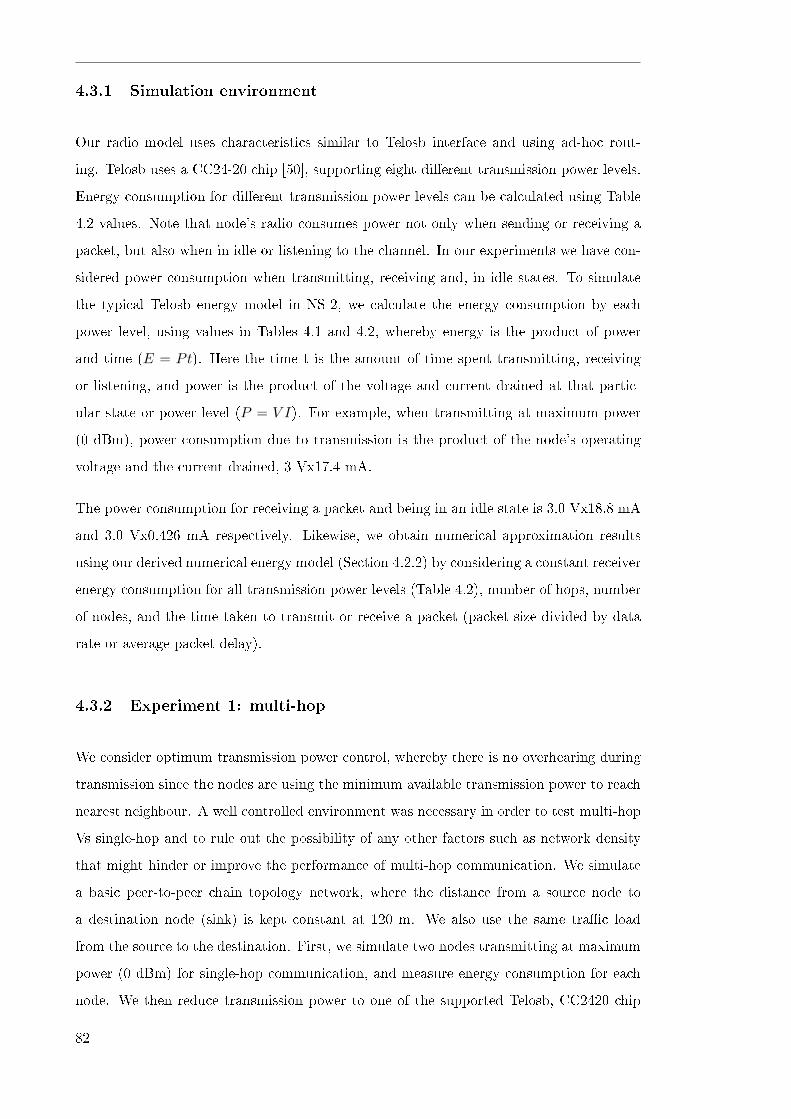
4.3.1 Simulation environment
Our radio model uses characteristics similar to Telosb interface and using ad-hoc rout-
ing. Telosb uses a CC24-20 chip [50], supporting eight di�erent transmission power levels.
Energy consumption for di�erent transmission power levels can be calculated using Table
4.2 values. Note that node's radio consumes power not only when sending or receiving a
packet, but also when in idle or listening to the channel. In our experiments we have con-
sidered power consumption when transmitting, receiving and, in idle states. To simulate
the typical Telosb energy model in NS-2, we calculate the energy consumption by each
power level, using values in Tables 4.1 and 4.2, whereby energy is the product of power
and time (E = Pt). Here the time t is the amount of time spent transmitting, receiving
or listening, and power is the product of the voltage and current drained at that partic-
ular state or power level (P = V I). For example, when transmitting at maximum power
(0 dBm), power consumption due to transmission is the product of the node's operating
voltage and the current drained, 3 Vx17.4 mA.
The power consumption for receiving a packet and being in an idle state is 3.0 Vx18.8 mA
and 3.0 Vx0.426 mA respectively. Likewise, we obtain numerical approximation results
using our derived numerical energy model (Section 4.2.2) by considering a constant receiver
energy consumption for all transmission power levels (Table 4.2), number of hops, number
of nodes, and the time taken to transmit or receive a packet (packet size divided by data
rate or average packet delay).
4.3.2 Experiment 1: multi-hop
We consider optimum transmission power control, whereby there is no overhearing during
transmission since the nodes are using the minimum available transmission power to reach
nearest neighbour. A well controlled environment was necessary in order to test multi-hop
Vs single-hop and to rule out the possibility of any other factors such as network density
that might hinder or improve the performance of multi-hop communication. We simulate
a basic peer-to-peer chain topology network, where the distance from a source node to
a destination node (sink) is kept constant at 120 m. We also use the same tra�c load
from the source to the destination. First, we simulate two nodes transmitting at maximum
power (0 dBm) for single-hop communication, and measure energy consumption for each
node. We then reduce transmission power to one of the supported Telosb, CC2420 chip
82

Table 4.1: Simulation parameter settings
Parameter Value
Channel carrier
frequency
2450 MHz
Data packet size 100 bytes, 28 bytes
Channel rate 250 kbpsData rate 12 kbps
RXthresh_ -94 dB
Max Queue length 256
Antenna gain 0
Simulation area 250m x 250m
Simulation time 24,000 seconds
Radio propagation
model
Freespace and
re�ection
Transmission power
(Pt_)
0,-1,-3,-5,-7,-10,-15,-25
dB
macSuperframeOrder
(SO)
15
macBeaconOrder (BO) 15
macMinBE 3
macMaxBE 5
macMaxCSMABacko�s 4
macMaxFrameRetries 3
Symbol interval 16µs
aUnitBacko�Period 20 symbols (320µs)
Current consumption in
transmit mode
depending on the
transmission power
(see Table 4.2)
Current consumption in
receiving mode
18.8 mA
Current consumption in
idle mode
0.426 mA
Typical node working
voltage
3.0 V
Table 4.2: Telosb transmission power and current
PA_level Output
power(dBm)
Current
drained
(mA)
31 0 17.4
27 -1 16.5
23 -3 15.2
19 -5 13.9
15 -7 12.5
11 -10 11.5
7 -15 9.4
3 -25 8.5
83

Figure 4.1: Chain ad-hoc scenario
power levels. This will automatically reduce the node's communication range. To maintain
the link between the source and the sink, which are 120 m apart, a node is strategically
placed between the source and sink, and transmission power is adjusted to establish a two
hop communication link (Figure 4.1). This process is repeated for other lower power level
values and more intermediate nodes are strategically placed between the source and the
sink, thus increasing the number of hops between them. The range between nodes, and
transmission power levels, can be approximated using propagation models, whereby Pr is
the node constant receiver sensitivity (-94 dBm). Furthermore, we maintain reasonably
low (12 kbps) source node data sending rate to avoid packet loss due to a queue over�ow.
This is a basic topology but it is quite su�cient to show the basic characteristics of trans-
mission power control in a multi-hop communication.
4.3.3 Experiment 2: single-hop
We simulate a pair of transmitter-receiver nodes, such that the distance from the transmit-
ter to the receiver is small enough to enable the use of the lowest power level (Table 4.2) to
transmit packets and therefore the radiation part remains constant. Using the same tra�c
load and same Tx/Rx range, we measure energy consumption for sending packets at di�er-
ent power levels. Again the radiation part will remain constant. The energy consumption
using the lowest level will obviously be minimum, however, we want to �nd by how much
this contributes to the energy savings and to compare our simulation and numerical results.
4.3.4 Results
Figure 4.2 shows numerical and simulation results for average energy consumed per packet
for each node as the number of hops increases.
84
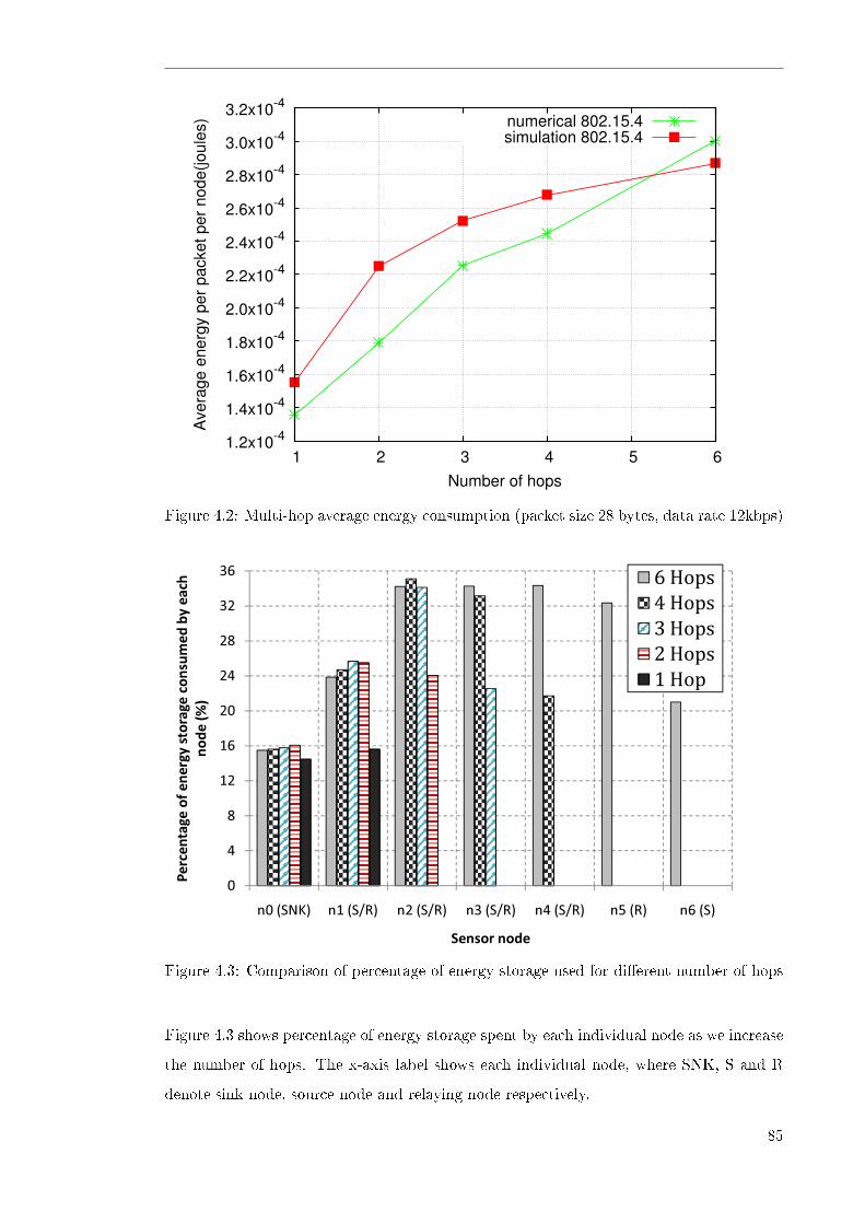
1.2x10⁻⁴
1.4x10⁻⁴
1.6x10⁻⁴
1.8x10⁻⁴
2.0x10⁻⁴
2.2x10⁻⁴
2.4x10⁻⁴
2.6x10⁻⁴
2.8x10⁻⁴
3.0x10⁻⁴
3.2x10⁻⁴
1 2 3 4 5 6
Ave
rage
ene
rgy
per p
acke
t per
nod
e(jo
ules
)
Number of hops
numerical 802.15.4simulation 802.15.4
Figure 4.2: Multi-hop average energy consumption (packet size 28 bytes, data rate 12kbps)
�
�
��
��
��
��
��
��
��
����������������� ������� ����������
������
������
������
������
�����
����
�
�
���� � ������ ������ ������ ������ ���� ����
����������������� ������� ����������
�����������
Figure 4.3: Comparison of percentage of energy storage used for di�erent number of hops
Figure 4.3 shows percentage of energy storage spent by each individual node as we increase
the number of hops. The x-axis label shows each individual node, where SNK, S and R
denote sink node, source node and relaying node respectively.
85

0.0x100
5.0x10⁻⁵
1.0x10⁻⁴
1.5x10⁻⁴
2.0x10⁻⁴
2.5x10⁻⁴
3.0x10⁻⁴
-25 -20 -15 -10 -5 0
Ave
rage
ene
rgy
cons
umed
per
nod
e pe
r pa
cket
(Jo
ules
)
Transmission power (dBm)
simulation 802.15.4analytical 802.15.4
Figure 4.4: Average energy consumption per node per packet (single-hop, data rate 64kbps,packet size 100 bytes)
Figure 4.4 shows average amount of energy consumed per packet for each node as a function
of transmission power.
86
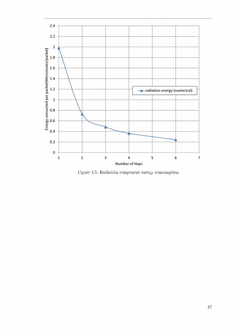
���
���
���
�
���
���
���
���
�
���
���
������������ ����������������������������
���� �������������������
�
���
� � � � � � �
������� ��� !�
Figure 4.5: Radiation component energy consumption
87
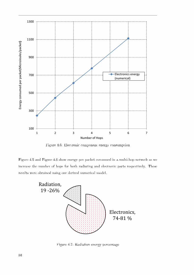
���
���
���
���
����
���������������� ����������������������������
���� ���������
���������
���
� � � � � � �
������ ��� ��
Figure 4.6: Electronic component energy consumption
Figure 4.5 and Figure 4.6 show energy per packet consumed in a multi-hop network as we
increase the number of hops for both radiating and electronic parts respectively. These
results were obtained using our derived numerical model.
�����������
������
���������
�������
�����������
������
���������
�������
Figure 4.7: Radiation energy percentage
88

Figure 4.7 shows the amount of energy contributed by radiation and electronics part using
di�erent transmission power levels in a single-hop experiment.
�
��
��
��
��
��
Ave
rage
pac
ket d
elay
(m
s)
�
� � � � � �
Number of hops
Figure 4.8: Delay comparison
Figure 4.8 shows the average end to end transmission delay as we increase number of hops.
This can be a major network degradation for time critical applications and for sensor nodes
with low memory or bu�er size.
89

��
���
�����������������������������A
vera
ge n
umbe
r of
col
lisio
ns
� � � ������ � � � �Number of hops
Figure 4.9: Number of collisions at the MAC/PHY layer versus number of hops
Figure 4.9 shows the average number of collisions versus the number of hops in a multi-hop
experiment.
4.4 Discussion
Other researchers [31, 32, 33] anticipated a bene�t of using multi-hop instead of single-hop
by suggesting that nodes in multi-hop can share the load, i.e. energy consumed sending
information will be shared among nodes in multi-hop resulting into lower energy per node
cost and longer lifetime. We agree with this �ndings if one only considers the energy
spent due to radiation or propagation or if the radiation part dominates the total energy
consumption (Figure 4.5 and 4.7) and not the node's electronics component (Figure 4.6
and 4.7).
Our �ndings con�rm that using TPC short-range multi-hop instead of single-hop does
not prolong nodes' lifespan in this case (Figure 4.2. and Figure 4.3). We used our well
controlled environment for testing, and derived numerical model and simulation results
to support our �ndings. Using multi-hop will increase coverage due to limited sensor
node ranges but not save energy. There can be several reasons why multi-hop short-range
90

fails to reduce the power consumption: energy is consumed by node's electronics not only
when sending packets but also when receiving packets; the International Organization for
Standardization (ISO) communication stack and layered protocols interact as the packet
transverses from one node to another, for example, the CSMA/CA in MAC sublayer is
performed per packet and per hop as packets go through several hops. Furthermore, by
increasing number of hops, we increase the number of nodes contending in the channel
and the number of nodes that cannot hear one another; this increases the chance of packet
collisions due to hidden terminals (Figure 4.9). Furthermore, by increasing the number of
hops we increase packet delay (Figure 4.8). Depending on the application tra�c, sensor
nodes' bu�er size can also cause performance degradation as we increase the number of
hops. Using our approach, results presented in this chapter can be related to those found
in [99].
TPC is e�ective in single-hop cellular or star networks and can increase the network's
lifespan because the power level can be changed based on single-hop receiver or sink prox-
imity (radiation part remains constant) and no other complexity exists compared to the
multi-hop case (Figure 4.4). This has been recognized for many years [100, 74, 96, 101].
Furthermore, TPC has been used in cellular networks for controlling co-channel interfer-
ence among devices in the shared radio channel [101]. In Figure 4.4, if we compare energy
spent when sending at the maximum power level (0 dBm) and the lowest power level (-
25 dBm); it shows that we can save energy by up to 23% compared to the single level
maximum transmission power.
These results suggest that a cluster based (hybrid topology) or similar topology would be
preferable. Instead of having every node relay the information, speci�c nodes would be
responsible for relaying the information and sensor nodes will pass the message in one hop
to the cluster head or relaying node which will not have the same energy restrictions as
the sensors nodes. Each node associated with a cluster head or relaying node will control
transmission power based on its distance from the cluster head or relaying node.
Our numerical model gives only an approximation of the results, it does not include other
control packets such acknowledgment, PAN association and retransmitted packets. It also
lacks the analysis of the energy spent due to the random nature of CSMA/CA. These
components are incorporated in our simulation results. Future work will include other
sources of energy consumption in the numerical model or analysis and results from a
hardware-based testing platform.
91

4.5 Conclusion
WSNs is a burgeoning area of research with many challenges, including managing energy
consumption and network connectivity. In this chapter, a new approach to transmission
power control was presented for multi-hop and single-hop WSNs. While some researchers
have suggested that short-range multi-hop communication can extend the sensor node's
lifespan, our results, both numerical and simulation, di�er from those �ndings. The re-
search showed that if the distance between source and destination is �xed, then the total
energy consumption in the WSN, packet collisions and packet delay all increase as we
increase the number of hops and reduce the transmission power for each hop. Results
indicate that, in a simulation scenario when a single-hop is used in conjunction with op-
timization of the transmission power, the node's energy consumption decreases by up to
23%. The di�erence between our results and the published literature is due to the fact that
we consider most components of energy consumption and not just the component related
to the power radiating from antennas. Furthermore, we used a basic simulation scenario
that is e�ectively maintained to test TPC in multi-hop communication.
92

Chapter 5
Association and Synchronization E�ciency
A key aspect of a wireless sensor network is its ability to self-organize and
maintain connectivity. Medium Access Control (MAC) protocol manages net-
work self-con�guration, which includes establishing a personal area network
(PAN), �nding a network to associate or disassociate with, and synchronizing
if required. Currently, there is limited research that addresses the network
initialization phase. This chapter provides a performance evaluation of the
802.15.4 MAC during device association and synchronization with the PAN co-
ordinator; this shows the impact of beacon interval is shown for the number of
associating nodes in terms of association time delay and energy consumption in
stationary wireless sensor networks. Results illustrate that energy consumption
and association time increase with increasing number of nodes associating with
a coordinator. Moreover, short beacon intervals consume more energy due to
the frequency of beacon frames that nodes have to keep track of to maintain
synchronization. However, short beacon intervals reduce the time required for
the nodes to associate, in contrast to longer beacon intervals that are unde-
sirable for real time and mobile applications. Furthermore, for longer beacon
intervals, BO= 12 to BO=14, there is an abrupt increase in energy consump-
tion as the number of associating nodes increase, even for as few as four nodes
as supposed to many expected nodes in sensor networks.
93

5.1 Introduction
Wireless Sensor Networks (WSN) are a major technology that promises solutions for various
industrial and domestic applications. A typical WSN is a distributed network formed by
sensor nodes deployed in a certain geographical region to collect and disseminate data.
Generally, the network will be composed of many scattered sensor nodes, from which data
will be routed from the original sensors to a remote sink in a single or multi-hop ad hoc
fashion. A typical WSN node (also referred to LR-WPAN platform) is composed of a
sensing module, a radio communication interface or transceiver module, a data processing
module, and a limited power supply module. The sensing module would most likely have
multiple on-board sensors for environmental variables such as temperature and humidity.
The data processing module is composed of a controller or microcontroller to process
all relevant data and codes. Usually the memory is a component of the data processing
module for storing programs and data. The power supply module may be battery or power
generator; however, often it will be quite limited. Generally, sensor nodes have serious
resource constraints including battery life, communication bandwidth, CPU capacity, and
storage [22].
This chapter focuses on the IEEE 802.15.4 standard for WSNs. The research provides a
study of the 802.15.4 standard the during the nodes' association and synchronization stage
in terms of synchronization time and energy consumption for a particular beacon interval.
Currently, insu�cient work has been done in the area of network initialization, i.e., as-
sociation and synchronization. Most research focuses on the performance of the 802.15.4
standard after the nodes' association and synchronization stage, during contention access
period (CAP) of the 802.15.4, by evaluating and analyzing 802.15.4 MAC CSMA/CA. In
[102, 103, 104, 105], the authors have developed mathematical models based on Markov
chains to analyze the performance of CSMA/CA. In [106], the suitability of 802.15.4 in mo-
bile networks was tested with respect to beacon order and node speed. Since the standard
has been designed for LR-WPAN with minimum complexity, performance degradation for
sophisticated mobile WSNs is expected. In this chapter , we consider stationary sensor
nodes and evaluate the performance of 802.15.4 based on beacon order and the number
of nodes associating with the PAN coordinator. Fan & et al [107] presented an improved
association scheme by reducing the number signaling between the PAN coordinator and
devices, thus shortening the total time to join the PAN to 0.20438 seconds compared to
the 0.5752 seconds obtained while using the 802.15.4 standard scheme. The authors used
94

�xed time values for every stage of association with a PAN coordinator and subtracted the
�xed time values for every stage that is redundant for an improved scheme. This approach
does not address the random nature of the association procedure as the values are �xed.
The 0.5752 seconds value reported is actually the scanning channel time and not the total
association time (section 5.3). Furthermore, in [107], the results do not include the impact
of beacon interval, as the authors used �xed beacon interval, i.e. beacon order (BO) equal
to three, and the study does not assess the impact of increased number of PAN coordinator
associating nodes as occurs in this study.
This appears to be the �rst investigation of the performance of the 802.15.4 MAC beacon
interval setting and the number of associating nodes. The performance evaluation is based
on the number of nodes associating with a coordinator and beacon intervals in terms of the
time required for a node to associate with its coordinator (association delay) and energy
consumed by a node to associate and synchronize with the coordinator.
The rest of the chapter is organized as follows. Section 5.2 introduces the IEEE 802.15.4
standard. In section 5.3, an overview of PAN creation is presented, and node association
and synchronization procedures. In Section 5.4 presents the performance simulation results
for IEEE 802.15.4 (beacon-enabled and non-beacon-enabled modes) in terms of synchro-
nization or association energy consumption and association time delay. In section 5.5, the
discussion of the signi�cance of our �ndings and future research directions. Finally, chapter
conclusions are drawn in section 5.6.
5.2 The IEEE 802.15.4 Standard
The IEEE 802.15.4 standard describes the Physical layer (PHY) and medium access con-
trol (MAC) sublayer speci�cations for wireless communication particularly for low-rate,
low-power consumption, wireless, personal area networks (LR-WPANs) [7]. The standard
has been designed with low complexity and cost wireless connectivity, making it a greatly
anticipated technology for wireless sensor networks (WSNs). A PAN involves one coordi-
nator which manages the whole network, but may involve one or more coordinators for a
network's subset nodes. The standard supports star, cluster- tree and mesh (peer-to-peer)
network topologies. This chapter considers only the star topology investigation.
In the IEEE 802.15.4 speci�cations, network devices can be classi�ed as full-function
95
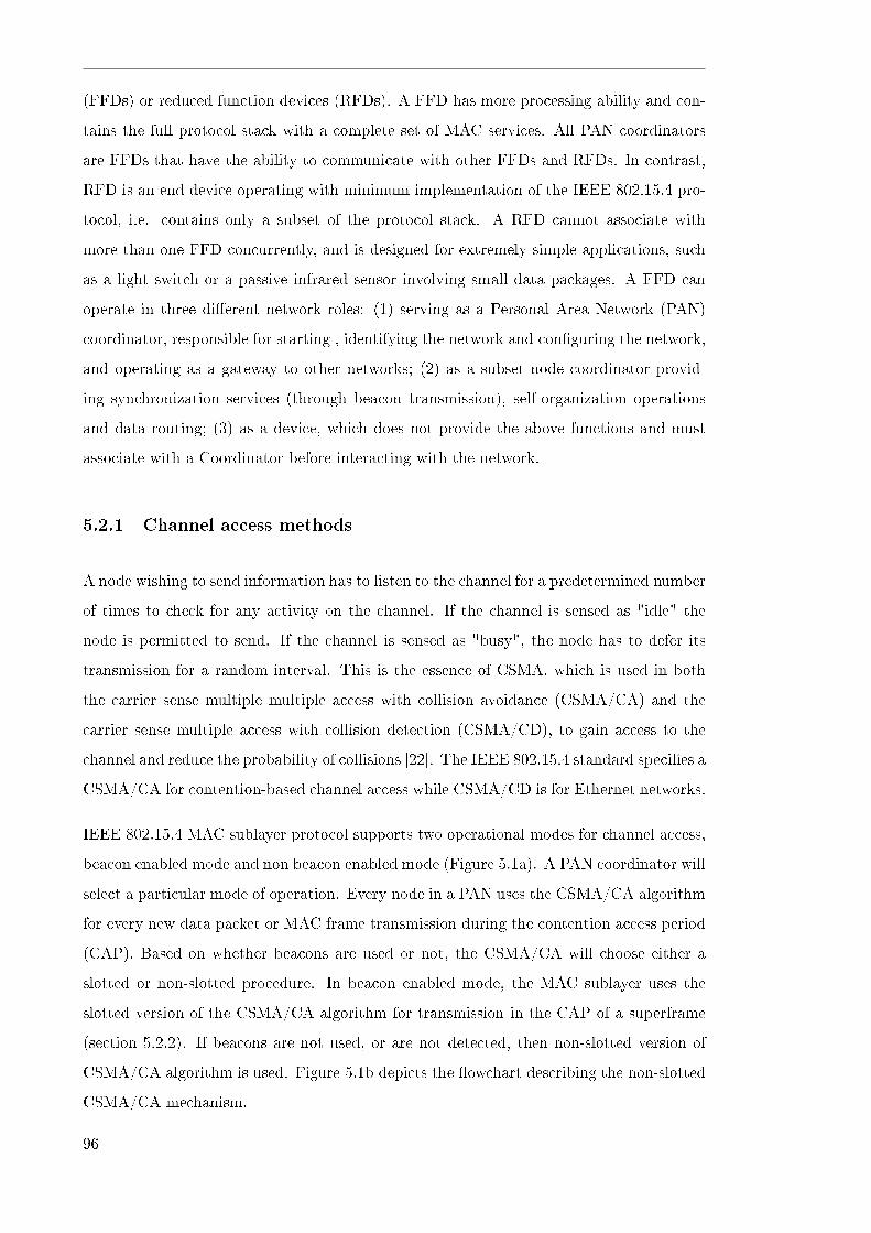
(FFDs) or reduced function devices (RFDs). A FFD has more processing ability and con-
tains the full protocol stack with a complete set of MAC services. All PAN coordinators
are FFDs that have the ability to communicate with other FFDs and RFDs. In contrast,
RFD is an end device operating with minimum implementation of the IEEE 802.15.4 pro-
tocol, i.e. contains only a subset of the protocol stack. A RFD cannot associate with
more than one FFD concurrently, and is designed for extremely simple applications, such
as a light switch or a passive infrared sensor involving small data packages. A FFD can
operate in three di�erent network roles: (1) serving as a Personal Area Network (PAN)
coordinator, responsible for starting , identifying the network and con�guring the network,
and operating as a gateway to other networks; (2) as a subset node coordinator provid-
ing synchronization services (through beacon transmission), self-organization operations
and data routing; (3) as a device, which does not provide the above functions and must
associate with a Coordinator before interacting with the network.
5.2.1 Channel access methods
A node wishing to send information has to listen to the channel for a predetermined number
of times to check for any activity on the channel. If the channel is sensed as "idle" the
node is permitted to send. If the channel is sensed as "busy", the node has to defer its
transmission for a random interval. This is the essence of CSMA, which is used in both
the carrier sense multiple multiple access with collision avoidance (CSMA/CA) and the
carrier sense multiple access with collision detection (CSMA/CD), to gain access to the
channel and reduce the probability of collisions [22]. The IEEE 802.15.4 standard speci�es a
CSMA/CA for contention-based channel access while CSMA/CD is for Ethernet networks.
IEEE 802.15.4 MAC sublayer protocol supports two operational modes for channel access,
beacon enabled mode and non beacon enabled mode (Figure 5.1a). A PAN coordinator will
select a particular mode of operation. Every node in a PAN uses the CSMA/CA algorithm
for every new data packet or MAC frame transmission during the contention access period
(CAP). Based on whether beacons are used or not, the CSMA/CA will choose either a
slotted or non-slotted procedure. In beacon enabled mode, the MAC sublayer uses the
slotted version of the CSMA/CA algorithm for transmission in the CAP of a superframe
(section 5.2.2). If beacons are not used, or are not detected, then non-slotted version of
CSMA/CA algorithm is used. Figure 5.1b depicts the �owchart describing the non-slotted
CSMA/CA mechanism.
96
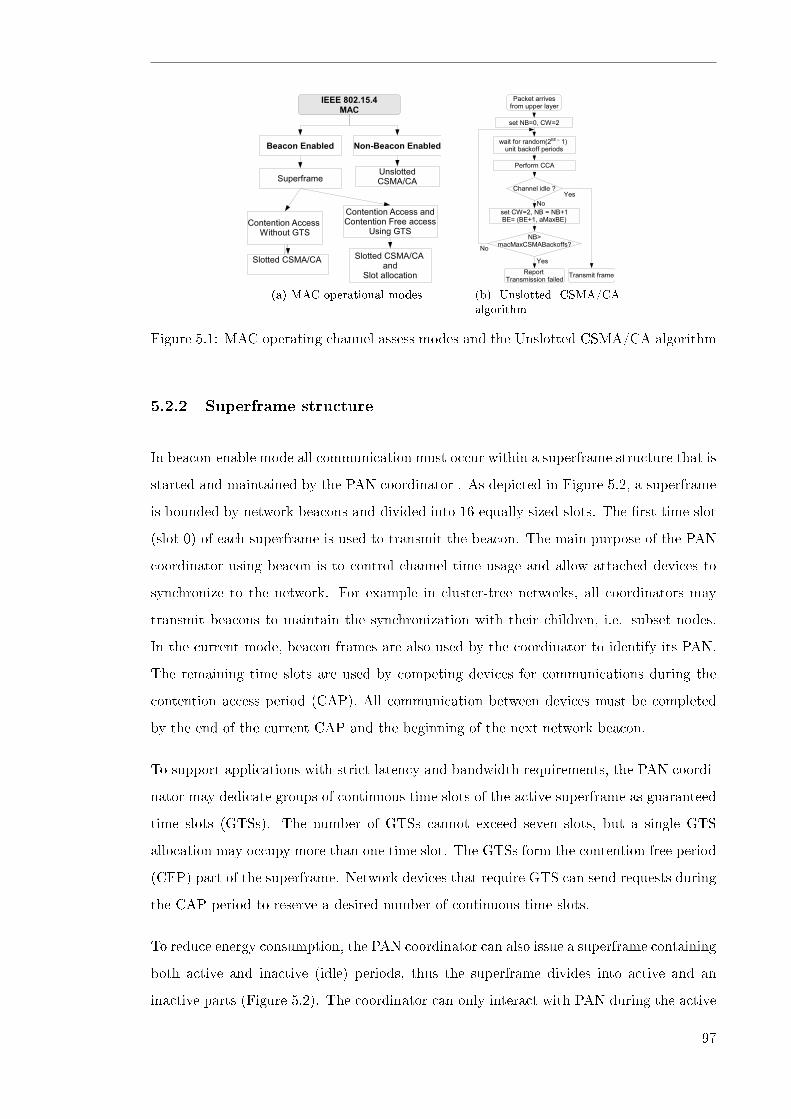
(a) MAC operational modes (b) Unslotted CSMA/CAalgorithm
Figure 5.1: MAC operating channel assess modes and the Unslotted CSMA/CA algorithm
5.2.2 Superframe structure
In beacon-enable mode all communication must occur within a superframe structure that is
started and maintained by the PAN coordinator . As depicted in Figure 5.2, a superframe
is bounded by network beacons and divided into 16 equally sized slots. The �rst time slot
(slot 0) of each superframe is used to transmit the beacon. The main purpose of the PAN
coordinator using beacon is to control channel time usage and allow attached devices to
synchronize to the network. For example in cluster-tree networks, all coordinators may
transmit beacons to maintain the synchronization with their children, i.e. subset nodes.
In the current mode, beacon frames are also used by the coordinator to identify its PAN.
The remaining time slots are used by competing devices for communications during the
contention access period (CAP). All communication between devices must be completed
by the end of the current CAP and the beginning of the next network beacon.
To support applications with strict latency and bandwidth requirements, the PAN coordi-
nator may dedicate groups of continuous time slots of the active superframe as guaranteed
time slots (GTSs). The number of GTSs cannot exceed seven slots, but a single GTS
allocation may occupy more than one time slot. The GTSs form the contention free period
(CFP) part of the superframe. Network devices that require GTS can send requests during
the CAP period to reserve a desired number of continuous time slots.
To reduce energy consumption, the PAN coordinator can also issue a superframe containing
both active and inactive (idle) periods, thus the superframe divides into active and an
inactive parts (Figure 5.2). The coordinator can only interact with PAN during the active
97
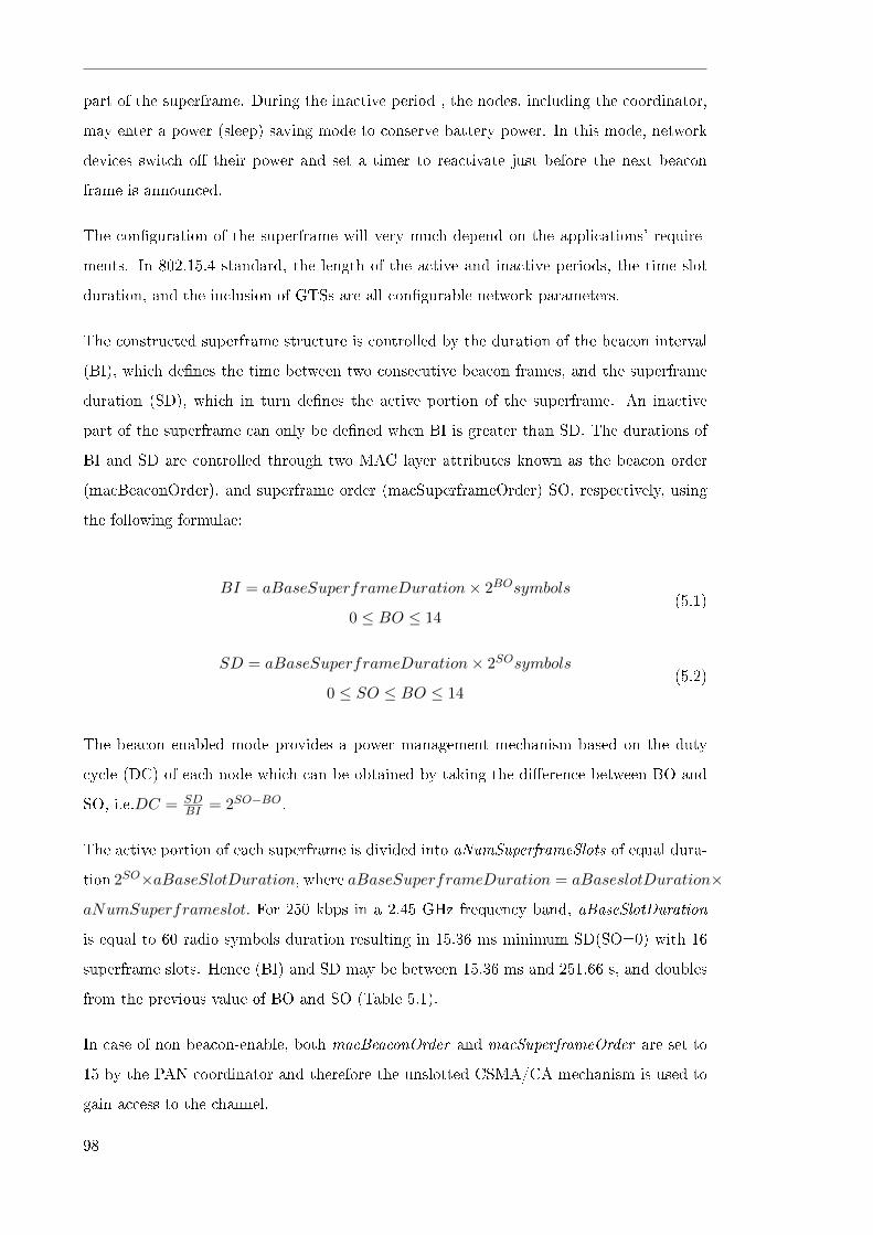
part of the superframe. During the inactive period , the nodes, including the coordinator,
may enter a power (sleep) saving mode to conserve battery power. In this mode, network
devices switch o� their power and set a timer to reactivate just before the next beacon
frame is announced.
The con�guration of the superframe will very much depend on the applications' require-
ments. In 802.15.4 standard, the length of the active and inactive periods, the time slot
duration, and the inclusion of GTSs are all con�gurable network parameters.
The constructed superframe structure is controlled by the duration of the beacon interval
(BI), which de�nes the time between two consecutive beacon frames, and the superframe
duration (SD), which in turn de�nes the active portion of the superframe. An inactive
part of the superframe can only be de�ned when BI is greater than SD. The durations of
BI and SD are controlled through two MAC layer attributes known as the beacon order
(macBeaconOrder), and superframe order (macSuperframeOrder) SO, respectively, using
the following formulae:
BI = aBaseSuperframeDuration× 2BOsymbols
0 ≤ BO ≤ 14(5.1)
SD = aBaseSuperframeDuration× 2SOsymbols
0 ≤ SO ≤ BO ≤ 14(5.2)
The beacon enabled mode provides a power management mechanism based on the duty
cycle (DC) of each node which can be obtained by taking the di�erence between BO and
SO, i.e.DC = SDBI = 2SO−BO.
The active portion of each superframe is divided into aNumSuperframeSlots of equal dura-
tion 2SO×aBaseSlotDuration, where aBaseSuperframeDuration = aBaseslotDuration×
aNumSuperframeslot. For 250 kbps in a 2.45 GHz frequency band, aBaseSlotDuration
is equal to 60 radio symbols duration resulting in 15.36 ms minimum SD(SO=0) with 16
superframe slots. Hence (BI) and SD may be between 15.36 ms and 251.66 s, and doubles
from the previous value of BO and SO (Table 5.1).
In case of non beacon-enable, both macBeaconOrder and macSuperframeOrder are set to
15 by the PAN coordinator and therefore the unslotted CSMA/CA mechanism is used to
gain access to the channel.
98
A beacon is transmitted without the use of CSMA, at the start of slot 0, followed by
CAP and CFP to the end of the superframe's active part. As with the beacon, CAP is
a mandatory part of a superframe. Coordinators are required to listen to the channel for
the whole CAP to detect and receive any data from their child nodes. Conversely, the
child node may only transmit data and receive an optional acknowledgment (ACK) when
needed, thus increasing their energy e�ciency.
All superframe settings are sent to network devices through beacon frames (Figure 5.4).
In the superframe speci�cation �eld (Figure 5.4), beacon order, superframe order, number
of CAP slots, power saving settings, PAN coordinator bit and association permit bit are
speci�ed [7].
Table 5.1: Superframe duration
BO/SO BI/SD BO/SO BI/SD BO/SO BI/SD
0 15.36ms 5 491.52ms 10 15.72864s
1 30.72ms 6 983.04ms 11 31.45728s
2 61.44ms 7 1.96608
s
12 62.91456s
3 122.88ms 8 3.93216s 13 125.82912s
4 245.76ms 9 7.86432s 14 251.65824s
Figure 5.2: Superframe format
5.3 Initialization of a PAN Coordinator, Node Association
and Synchronization
One key aspect of a wireless sensor network is its ability to self-organize and maintain
connectivity. The MAC protocol manages the self con�guration of the network, i.e., ability
99
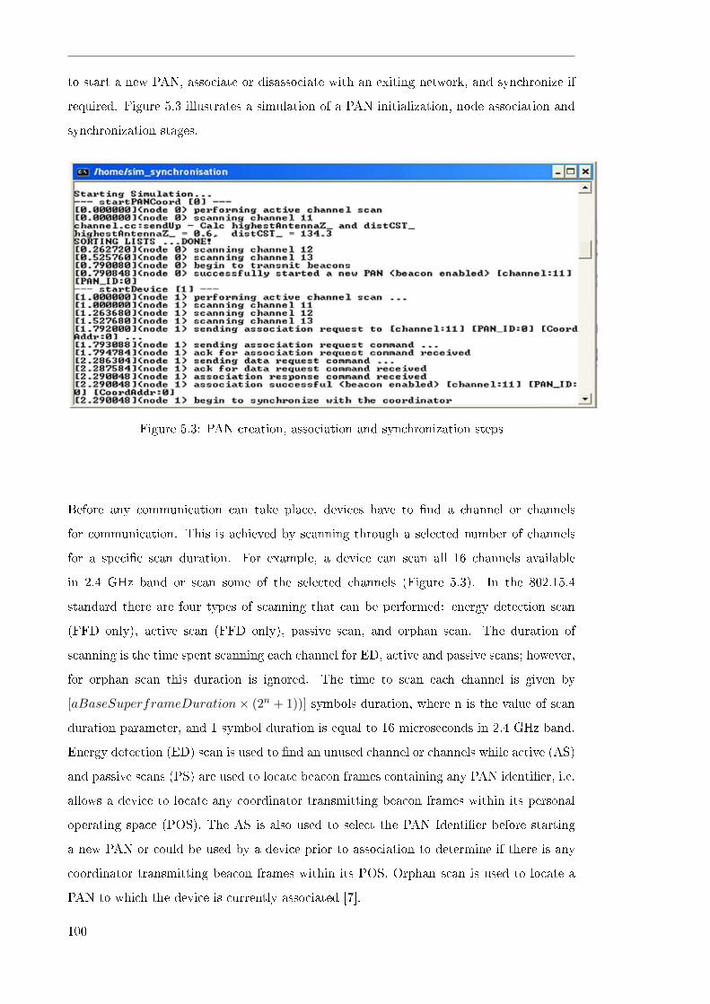
to start a new PAN, associate or disassociate with an exiting network, and synchronize if
required. Figure 5.3 illustrates a simulation of a PAN initialization, node association and
synchronization stages.
Figure 5.3: PAN creation, association and synchronization steps
Before any communication can take place, devices have to �nd a channel or channels
for communication. This is achieved by scanning through a selected number of channels
for a speci�c scan duration. For example, a device can scan all 16 channels available
in 2.4 GHz band or scan some of the selected channels (Figure 5.3). In the 802.15.4
standard there are four types of scanning that can be performed: energy detection scan
(FFD only), active scan (FFD only), passive scan, and orphan scan. The duration of
scanning is the time spent scanning each channel for ED, active and passive scans; however,
for orphan scan this duration is ignored. The time to scan each channel is given by
[aBaseSuperframeDuration× (2n + 1))] symbols duration, where n is the value of scan
duration parameter, and 1 symbol duration is equal to 16 microseconds in 2.4 GHz band.
Energy detection (ED) scan is used to �nd an unused channel or channels while active (AS)
and passive scans (PS) are used to locate beacon frames containing any PAN identi�er, i.e.
allows a device to locate any coordinator transmitting beacon frames within its personal
operating space (POS). The AS is also used to select the PAN Identi�er before starting
a new PAN or could be used by a device prior to association to determine if there is any
coordinator transmitting beacon frames within its POS. Orphan scan is used to locate a
PAN to which the device is currently associated [7].
100

5.3.1 PAN Creation
To start any PAN, the �rst step involves establishing a PAN coordinator. Any FFD can be
the sole PAN coordinator. The following is a summary of the steps used when establishing
a PAN coordinator (creating a new PAN):
1. Upon power up, a FFD transceiver may begin ED scan and then an active scan on each
of the available channels to �nd a suitable frequency for communicating within its personal
operating space (POS)
2. During active scan (AS), a device sends out a beacon request command and then sets a scan
duration
3. If no beacon is detected within the scan duration, the FFD believes that there is no coordi-
nator in its POS
4. The PAN coordinator will lock on a suitable channel, select an identi�cation number for
the PAN known as the PANid, assign itself a short address (less than 0x��), and begin to
operate as a PAN coordinator by broadcasting its periodic beacon frame. At this stage the
superframeOrder beaconOrder parameters are set and now devices can associate with the
PAN coordinator. The PAN coordinator will control device association by assigning short
addresses to devices and coordinators
5.3.2 PAN Association and Synchronization
A FFD or RFD device can request to join an existing PAN within its POS by initializing an
association procedure. In order to optimize the association procedure on a beacon-enabled
PAN, a device is allowed to start tracking the beacon of the coordinator of interest in
advance[7]. The following is a summary of the steps used when a device wants to associate
with an existing PAN (section 5.3.1):
1. Device's PAN association starts with a device performing either an active or passive channel
scan to determine if there is any coordinator transmitting beacon frames within its POS.
It also has to �nd a PAN coordinator that is accepting incoming association requests when
using an AS. For passive scan the beacon request command is not required
2. From scan results above, if a PAN coordinator/s exists the device will select a suitable PAN
and attempt to join a PAN as long as PAN coordinator allows association (Figure 5.4), as
determined through the scan procedure. A device can then transmit an association request
command for an association with a coordinator
101

3. The coordinator will then send an acknowledgment frame con�rming that it received the
request command and then make a decision within aResponseWaitTime symbols duration
(aResponseWaitT ime = 32 ∗ aBaseSuperframeDuration symbols = 30,720 symbols ≈
0.49s) as to whether to allow association or not. This decision will depend on whether there
are su�cient resources available
4. For beacon-enabled mode, the device will wait for the maximum aResponseWaitTime sym-
bols duration for the coordinator to make the decision. Within aResponseWaitTime symbols
duration, the device will seek information about the decision made by the coordinator when-
ever a beacon frame appears. In the case of a non-beacon enabled mode, the device will seek
the association response command after aResponseWaitTime symbols duration. If there is
no response, the association attempt has failed
5. On receiving the association response command, the device requesting association will send
an acknowledgment frame con�rming receipt. If the status of an association response com-
mand indicates the association was successful, the device will con�gure the PHY and MAC
attributes, to the value necessary for association (used when a device transmits data) that
include the channel to use (phyCurrentChannel), PANid (macPANid) and the short address
of the coordinator
Note that all devices in PAN, come with a pre-assigned long address, the PAN coordinator
must be assigned a short address to itself before it can allow the start request . A FFD
that is not a PAN coordinator can only begin transmitting beacon frames when it has
successfully associated with a PAN coordinator (Figure 5.3).
Once devices have associated with the coordinator, all devices will be allowed to acquire
beacon synchronization only with beacons containing the PAN identi�er speci�ed in mac-
PANId. If macPANId speci�es the broadcast PAN identi�er (0 x ��), a device shall not
attempt to acquire beacon synchronization. All devices operating in a beacon-enabled
PAN (i.e., macBeaconOrder<15) have to maintain beacon synchronization to detect any
pending messages or to track the beacon. Synchronization is maintained by all devices
by receiving and extracting beacon frames (Figure 5.4). All devices operating on a non
beacon-enabled PAN (macBeaconOrder=15) must be able to poll the coordinator for data
at the discretion of the next higher layer (5.2.2).
102

Figure 5.4: Beacon frame format
5.4 Performance Evaluation
To observe the impact of beacon interval (BI) and number of nodes associating with the
PAN coordinator, we obtained the average energy consumed per node to associate and
synchronize with the coordinator, and the average time required by a node to associate
with the PAN coordinator.
5.4.1 Simulation model
NS-2 [82] simulator was used to study the impact of beacon interval and the non beacon
case during node association and synchronization. It involved a star network topology,
using 802.15.4 standard, where the sink node in the middle acts as the PAN coordinator
and all surrounding items are associating nodes. The PAN coordinator and associating
nodes are all stationary. All nodes in the ideal star topology are in range with the PAN
coordinator and there is no channel interference. The coordinator starts at 0.0 seconds,
followed by each associating node in turn, 1 second apart. Each simulation ran for 5000
seconds. No data are sent by nodes that have joined the PAN as we are interested with
the association and synchronization part only. Table 5.2 shows our simulation parameters.
5.4.2 Results
Figure 5.5 and Figure 5.6 show average node's association and synchronization time for
di�erent beacon interval (BI) as we increase the number of nodes associating to one PAN
coordinator.
103

Table 5.2: Simulation Parameter Settings
Parameter Value
Frequency Band 2400-2483.5 MHz
Channel Rate 250 kbps
macSuperframeOrder (SO) 0-15
macBeaconOrder (BO) 0-15
macSuperframeSlots 16
aBaseSlotDuration 60 symbols (960 µs)
Symbol interval 16µs
aUnitBacko�Period/slot duration
(Tslot)
20 symbols (320µs)
macAckWaitDuration 54 symbols (864µs)
aResponseWaitTime 30,720 symbols
(0.4915s)
SIFS 12 symbols (192µs)
ACK reception duration (Tack) 544µs
ACK timeout (Tacktout) 864µs
Current consumption in transmit mode
(@ 0 dBm)
17.4mA
Current consumption in receiving
mode
18.8 mA
Current consumption in idle mode 0.426 mA
Typical node working voltage 3.0V
Simulation area 150m x 150m
Simulation time 5,000 seconds
Number of random seeds per
simulation
50
��
��
��
��
��
��������������� ����������
����
����
����
����
����
����
����
���
�
�
��
��
� � � � � � � �
��������������� ����������
�������������
���
����
���������
Figure 5.5: Devices' PAN association and synchronization durations for beacon orders up to 8
and 15
104
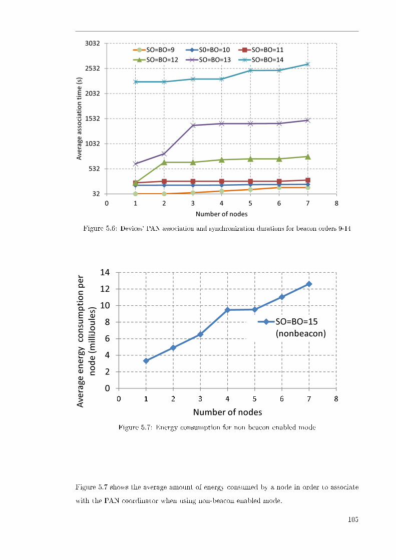
���
����
����
����
����
����
��������������� ����
�����
����� ������� �������
������� ������� �������
��
���
� � � � � � � �
���������������
Figure 5.6: Devices' PAN association and synchronization durations for beacon orders 9-14
�
�
�
�
�
��
��
��
������������������ �����������
������������� ����
������
����������
� � � � � � � � �
������������������ �����������
���������������
Figure 5.7: Energy consumption for non beacon enabled mode
Figure 5.7 shows the average amount of energy consumed by a node in order to associate
with the PAN coordinator when using non-beacon enabled mode.
105

�
��
��
��
��
������������������� ������������������� ����
���
���
���
��
���
���
���
�
�
� � � � � � � ������������������ ������������������� ����
��������������
���
���
Figure 5.8: Association and synchronization energy consumption
���
����
���
����
���
����������������� ������������������� ����
���
���
�����
�����
����
�����
��
�� �
� � � � � � �
����������������� ������������������� ����
���������������
�����
�����
Figure 5.9: Association and synchronization energy consumption
Figure 5.8 and Figure 5.9 show average energy consumption per node for di�erent BI as
we increase the number of nodes associating to one PAN coordinator when using beacon
enabled mode.
106

5.5 Discussion
Results illustrate that over a longer period, shorter beacon intervals will consume more
of the node's energy while long beacon intervals will require less energy. Short beacon
intervals consume more energy due to the frequency of beacon frames with which nodes
have to keep track of to maintain synchronization; our results suggest that this is valid
for BO=0 to BO= 11 (Figure 5.8 and Figure 5.9). However, for longer beacon intervals,
BO= 12 to BO=14, there is an abrupt increase in energy consumption as the number
of associating nodes increases, even for as few as four nodes. The energy consumption
increases in the order of about 1 millijoule for every additional associating node for all
beacon order (BO) values ranging from 0 to 11. Results also illustrate that non-beacon
mode consumes less energy to associate to the PAN coordinator compared to the beacon
enabled. The main reason low association energy for non-beacon enabled mode is that
there is no beacon transmission to maintain synchronization as opposed to beacon enabled
mode (Figure 5.7).
The results demonstrate that the average node's association delay time increases with
increased number of nodes and increased beacon intervals (Figure 5.5 and Figure 5.6 ).
However, there is a very small time di�erence between non-beacon enabled PAN and beacon
enable PAN for values of beacon order (BO) between 0 and 4. Furthermore, our results
demonstrate that as the number of associating nodes increases, longer beacon interval
cases su�er longer association delays (Figure 5.6) compared to shorter beacon intervals,
and the energy consumption for association and synchronization increases. For example,
it will take about 42 minutes for 7 nodes requesting association to associate with the
coordinator, when BO=14. Such long beacon intervals are unsuitable for real time and
mobile WSN applications.
To conserve energy inWSNs, we expect to use longer beacon interval (BI) and shorter active
periods (SD) so that the nodes can go into inactive or sleep state during CAP to save energy.
To date the longest beacon interval is 251.66s (about 4 minutes). Our results demonstrate
that even with 7 nodes connected to the PAN coordinator, the association delay and energy
consumption due to synchronization, increase. The question is whether the association
energy consumption will outweigh the bene�t of duty cycle power management for larger
beacon intervals, as the number of associating nodes increases?
107

5.6 Conclusions
WSNs are a research hotspot with many challenges, including managing energy consump-
tion and network connectivity. In this chapter, performance evaluation of the 802.15.4
MAC beacon interval settings during devices' association and synchronization with the
PAN coordinator was presented. Overall, non-beacon mode consumes less energy to asso-
ciate to the PAN coordinator compared to beacon enabled.
It has been demonstrated that over a longer period, shorter beacon intervals will consume
more of the node's energy while long beacon intervals will spend less energy, at least for
BO=0 to BO=11. The associating energy consumption increases with increased number of
nodes for all beacon intervals (B0=0-15). For longer beacon intervals, BO=12 to BO=14,
there is an abrupt increase in energy consumption as the number of associating nodes
increases, even for a small number of nodes, such as four. Results demonstrate that it will
take about 42 minutes for 7 nodes requesting association to associate with the coordinator,
when BO=14. Such long delays are not suitable for real time and mobile WSN applications.
The question here is whether the association energy consumption will outweigh the bene�t
of duty cycle power management for larger beacon intervals as the number of associating
nodes increases. Future work will further investigate possible solutions to improve the
performance of 802.15.4 during PAN association and synchronization stage and during
data sending stage.
108
Chapter 6
Clear Channel Assessment and Enhanced MAC for
Hidden Nodes
The IEEE 802.15.4 MAC protocol standard controls radio channel access us-
ing the Carrier Sense Multiple Access with Collision Avoidance (CSMA/CA)
algorithm. To avoid collisions, the standard adjusts the backo� exponent (BE)
based on two consecutive clear channel assessments (CCA) before packet trans-
mission. The CCA part is carried out at the physical (PHY) layer, and used
by the MAC protocol as part of the CSMA/CA algorithm, whereby a node is
required to perform a CCA for a predetermined duration to determine if the
channel is available for transmission (i.e. check whether the channel is busy or
idle) before transmission of the data frame. This chapter provides an investiga-
tion on the impact of the number of times the CCA is performed in the 802.15.4
MAC sublayer during frame transmission; in terms of throughput, packet error
rate, delay, and energy consumption. The study considers both hidden and
non-hidden nodes in a network system. Results show a serious network perfor-
mance degradation, even for a small number of hidden nodes in a network. In
this chapter a proposed cross layer (PHY-MAC) design is presented, aimed at
improving network: energy e�ciency, reliability, and scalability; by reducing
packet collisions due to hidden terminals/nodes.
6.1 Introduction
The IEEE 802.15.4 standard describes the physical layer (PHY) and the medium access
control (MAC) sublayer speci�cations for wireless communication; in particular for low-
109
rate, low-power consumption, wireless personal area networks (LR-WPANs) [7]. The stan-
dard represents a signi�cant milestone in promoting deployment of wireless sensor networks
(WSNs) for a variety of commercial uses [108].
The MAC sublayer is a broad research area, however, this chapter focuses on the e�ciency
of the MAC sublayer for WSNs. Earlier studies have sought to improve WSNs in the area
of a power e�cient MAC sublayer[71, 18, 72, 73, 74, 77]. In [73], the authors developed
a power e�cient MAC protocol known as PAMAS. PAMAS was designed to reduce the
overhearing between nodes by using a separate signaling channel. The PAMAS method
requires an extra radio interface and therefore increases the hardware costs and the com-
plexity of the MAC sublayer for a sensor node. In [74], an extension to the standard 802.11
MAC protocol known as power control multiple access (PCMA) was presented. PCMA un-
like PAMAS, does not use a separate signaling channel, and can also be used by any other
protocols that use CSMA/CA. The main aim of the PCMA is to use less power compared
to the 802.11 standard, and still retain the same throughput. This was achieved by trans-
mitting DATA and acknowledgment (ACK) frames at the minimum transmission power,
and transmitting request-to-send (RTS) and clear-to-send (CTS) frames at the maximum
transmission power. Moreover, to reduce collisions, data transmissions are periodically
transmitted at maximum power, so neighboring nodes can sense the medium occupied,
and refrain from sending RTS frames.
Wei et al. [18] developed a power e�cient protocol known as S-MAC (schedule MAC),
which is a contention based MAC protocol like the IEEE 802.11 MAC protocol. However,
the main di�erence between them is the power saving mode of S-MAC, which adds power
saving features to the virtual carrier sense. When a NAV (Network Allocation Vector)
shows that the remaining time of the ongoing transmissions is nonzero, and that the
transmission does not involve the current node; the radio is powered o� until the NAV
reaches zero (Fig 6.4). The S-MAC design reduces the energy consumption caused by idle
listening, and tackles the overhearing problem by sending interfering nodes to sleep once
they hear a RTS/CTS signal; however latency is increased (tradeo� between energy and
latency), since the sending nodes must wait for the receiver to wake up before sending
out data [18]. In summary [18] identi�ed and described areas of energy wastage including:
idle listening, collisions, overhearing, and control overhead; and aimed to reduce energy
consumption, while supporting network scalability and collision avoidance.
Dam & Langendoen [75] presented another contention based MAC protocol called T-MAC
110

(Timeout MAC), which aims to reduce energy consumption by allowing active nodes to
have adaptive/variable duty-cycles rather than �xed ones. The design allows every node to
decide its own duty-cycle based on its activation period, and to end the active time upon
hearing nothing on the channel (for a period known as timeout). The T-MAC protocol
causes more latency in a network compared to the S-MAC protocol; however, the authors
claim to give much better energy performance results for low data rate applications. Both
T-MAC and S-MAC use periodic time synchronization that can consume a lot of energy.
B-MAC (Berkeley MAC) [76]is also a contention based MAC protocol, but is only a link
layer protocol design, with network services such as organisation, synchronisation, and
routing being built above its implementation. B-MAC performs carrier sensing using Clear
Channel Assessment (CCA), and the sleep/wake scheduling by using Low Power Listening
(LPL). Signi�cant B-MAC design considerations include: keeping MAC implementation
code size small for small storage, saving energy, and providing users with complete �exi-
bility to change di�erent MAC parameters, such as CCA, acknowledgments, backo�s, and
LPL to suit a particular WSN application. These changes can be made using the B-MAC
con�guration interface at run-time. Other advantages of this design include: no RTS/CTS
signalling requirement, and no synchronisation of packets requirement. However, the de-
sign causes a huge overhead because of overhearing, whereby receiver nodes have to stay
awake while receiving a long preamble, even when they are not the intended destinations.
Z-MAC (Zebra MAC) [77] is a hybrid MAC scheme that combines the strengths of CSMA
and time division multiple access (TDMA). The design allows nodes that are within inter-
ference range and in a high contention scenario to transmit during di�erent times/slots to
avoid collisions, i.e. it's collision free. However, unlike TDMA, a node can transmit during
any given time slot. T-MAC's main design goals are to reduce energy consumption, by
tackling frame collisions caused by hidden nodes, and controlling overhead frames such as
RTS/CTS or Data/ACK.
This chapter presents a study on the impact of the number of times the CCA is performed
in the 802.15.4 MAC during frame transmission; in terms throughput, packet error rate,
delay, and energy consumption. Both hidden and non-hidden nodes in a network system
are considered in the experiments, and a new cross layer (PHY-MAC) design is proposed.
The purpose of the new cross layer is to improve network energy e�ciency, interference,
reliability, and scalability; by minimising packet collisions due to hidden nodes. The pro-
posed changes can coexist with the legacy 802.15.4 CSMA/CA, and can also be used by
111
CSMA/CA MAC protocols.
6.2 IEEE 802.15.4 MAC Layer
The IEEE 802.15.4 MAC sublayer controls radio channel access using the Carrier Sense
Multiple Access with Collision Avoidance (CSMA/CA) mechanism. Every PAN node uses
the CSMA/CA algorithm for every data packet or MAC frame transmission during the
contention access period (CAP). This is achieved through the standard modes of operation:
beacon enabled and non-beacon enabled. The mode is selected by the central node (PAN
coordinator). In non-beacon enabled mode, the MAC protocol uses a simple non-slotted
CSMA/CA algorithm for transmission in the CAP, which requires constant reception for
potential incoming data. In beacon enabled mode, the MAC protocol uses a modi�ed
slotted CSMA/CA algorithm that requires all nodes to be synchronized through beacon
frames[7]. Based on whether beacons are used or not, the CSMA/CA will choose either
a slotted or non-slotted procedure. If beacons are not used, or are not detected, then
the non-slotted version of the CSMA/CA algorithm is used. The CSMA/CA algorithm
is not used during beacon and acknowledgment frame transmissions. The data frame is
transmitted during the contention free access (CFA) period, and the data frame quickly
follows the acknowledgment of a data request command. Figure 6.1 depicts the �owchart
describing slotted and non-slotted CSMA/CA mechanisms.
The 802.15.4 MAC protocol is also responsible for: �ow control via acknowledgment of
frame delivery; frame validation (as well as maintaining network synchronization); net-
work association and dissociation; administering device security; and the scheming of the
guaranteed time slot mechanism.
6.2.1 The CSMA/CA algorithm
A node, wanting to send information, �rst listens to the channel for a predetermined
amount of time to check for any activity. If the channel is sensed as "idle" then the
node can send. If the channel is sensed as "busy" the node defers its transmission for a
random interval. In both CSMA/CA and CSMA/CD, this technique allows access to the
112

Figure 6.1: Slotted (a) and non-slotted (b) CSMA/CA algorithm
113

channel while reducing the probability of collisions [46, 26]. The CSMA/CA is used by the
IEEE 802.15.4 standard for contention-based channel access, while CSMA/CD is used by
Ethernet networks.
The CSMA/CA mechanism is based on a basic time unit called a unit backo� period (BP)
or backo� slot [7]. Each backo� slot, aUnitBacko�Period, lasts for 20 symbols (80 bits);
equivalent to 320 microseconds in a 2.45 GHz frequency band. Any node that has a packet
ready to send has to wait for a randomly chosen number of slots (BP). This backo� period/-
counter is decremented by one at the beginning of every slot that follows. At the end of the
backo� period, the node performs a clear channel assessment (CCA) for a predetermined
period to monitor the channel status before sending the packet; i.e. to check whether the
channel is busy or idle. The channel sensing mechanism ensures that the channel is clear
of activity for a predetermined duration known as the contention window (CW) duration,
expressed in terms of backo� slots, before the node can attempt transmission. Similarly,
the CW begins from a speci�ed value (default 2), and is decremented by one at every idle
contention window slot until it reaches zero.
In order for a node to access the channel for a transmission attempt, the CSMA/CA
algorithm requires each node to maintain three counters: 1) NB, which is the number of
backo� attempts/trials (backo� stage) for a particular frame transmission, initialised to 0
before each new transmission attempt. 2) BE, which is the backo� exponent that de�nes
the uniformly distributed random number of backo� durations, for which a device has to
wait, before performing a CCA. In slotted PAN, if macBattLifeExt is set as FALSE, then
BE is initialised to the value of macMinBE; otherwise if macBattLifeExt is set as TRUE,
the BE value will be initialised to the value of macMinBE minus 2. In the 802.15.4 the
default BEmin is 3, and BEmax is 5. 3)CW, which is the contention window duration,
expressed in terms of backo� slots, de�ning the number of consecutive backo� periods for
which a channel needs to be silent before transmission can commence.
The 802.15.4 standard de�nes the default CW duration to be 2 backo� slots (640µs). The
slotted CSMA/CA algorithm can be summarized as follows (Figure 6.1):
1. A node initialises NB=0, CW=2, and BE=MacMinBE, and then locates the backo� period
boundary of the next backo� period.
2. A node delays for a random number of complete backo� periods/slots in the range 0 to
2BE − 1, i.e. Backo� time=Random([0-2BE − 1])×aUnitBacko� Period , before sensing the
114

channel. This randomly chosen counter or backo� period is decremented by one at the
beginning of every slot that follows, until the counter is zero; before sensing the channel.
3. A node requests the PHY layer to perform a CCA to sense the channel, i.e. check whether
the channel is busy or idle. In slotted CSMA/CA, the CCA starts on the backo� period
boundary; while in unslotted, the backo� starts immediately.
4. If the channel was sensed as �busy� in step 3, the value of CW will be reset to its original
value, e.g. CW=2; BE will be increased by one after each transmission fails until it reaches
a maximum value BEmax (default BEmax =5); NB will be incremented by one, ensuring
NB is less or equal to MacCSMABacko�s (the standard default=4), and then the algorithm
will return to step 2. If the value of NB is greater than macCSMABacko�s, CSMA/CA will
terminate with a channel access failure status and the current packet will be discarded. If
the channel was sensed as idle in step 3, we jump to the next step (step 5).
5. If the channel was previously sensed as idle (step 3), the MAC sublayer in a slotted CS-
MA/CA system will ensure that the speci�ed contention window has expired before com-
mencing transmission. To do this, the CW value is checked, if its value is not equal to zero,
the CW is decremented by one and the algorithm goes back to step 3. If its value is equal to
zero, then the frame will be transmitted and the process recommences (step 1) for another
data frame.
A frame transmission is considered to be a success or a failure (collision) depending on
whether an optional ACK frame is successfully received after the frame transmission.
To deal with such a problem, the 802.15.4 standard supports an optional retransmission
scheme based on acknowledgments and timeouts. When the retransmission mechanism is
enabled, the destination node must send an acknowledgment after receiving a correct data
frame. The acknowledgment will not be sent if a collision or corrupted frame reception
occurs. The sender will wait for an acknowledgment, and if it does not receive it within a
speci�ed period (timeout), a retransmission will be scheduled. The standard default max-
imum number of retransmissions (macMaxFrameRetries) is 3. If the maximum number
of retransmissions is reached, then the data frame will be dropped. This retransmission
scheme applies when a node fails to transmit a frame either: 1) due to �ve consecutive
busy channel outcomes, i.e. NB>macCSMABacko�s; or 2) due to collisions.
In the CSMA/CA algorithm, BE is the main parameter used in the backo� procedure,
to reduce or control the probability of a collision among contending nodes in a multiple
access, broadcast channel. This backo� procedure is sometimes known as a truncated
binary exponential backo� (BEB).
115

The CSMA/CA algorithm provides a distributed access mechanism in the sense that each
station independently executes the algorithm to decide whether to transmit in the given
time slot. In this regard 802.15.4 CSMA/CA is similar to IEEE 802.11 CSMA/CA; how-
ever, in the former, a backo� counter value for the device decreases automatically at every
slot until it become zero, regardless of the channel status (busy or idle), and then performs
a CCA. This is one of the power saving features of 802.15.4 wherein devices can conserve
power during the backo� period, in contrast to the conventional CSMA/CA mechanism
used in IEEE 802.11 WLANs [109]. Figure 6.2 shows the channel access timings for the
802.15.4 and the 802.11 basic access (without RTS/CTS).
Figure 6.2: IEEE 802.11 and IEEE 802.15.4 channel access
6.3 Hidden Terminals Problem
The wireless medium has some special properties that a�ect the performance of contention
based MAC protocols. The wireless receiver requires the received signal to meet a certain
minimum signal threshold/strength in order to be detected. Therefore, if the distance
between two stations exceeds some threshold, they cannot hear each other. Thus for
116

protocols incorporating carrier sensing (e.g. CSMA/CA) to be e�ective, detection time
and propagation delays in the system must be small; given that the user waits to transmit
a random time period after sensing the channel is free. The CSMA only works when all
users can detect each others transmissions (within range), and delays are small. However,
the nature of the wireless channel may prevent a given node from detecting the signal
transmitted by all other nodes, especially for nodes with low transmission/sensing range.
This gives rise to the hidden terminal scenario, as illustrated in Figure6.3
Consider three stations A, B, and C; with transmission radii as indicated by the solid
circles. Station B can communicate with both A and C since they are in range of B, but
A is not in the range of C, and vice versa. If C starts to transmit packets to B, A cannot
detect the transmission using the carrier sense mechanism, and considers the medium to be
free. Hence A also starts packet transmission and therefore a collision will occur at B. To
avoid packet collisions due to possible hidden terminals, techniques such as the one used in
the 802.11 standard networks, by using the four handshake request to send-clear to send
(RTS-CTS) exchange and furthermore use ACK for reliability, can be useful as illustrated
in Figure 6.4. All nodes that hear a RTS or CTS will not transmit for the duration of the
transfer. For example, in Figure 6.3, station A will hear the CTS sent by station B to C,
and therefore backo� to avoid collision.
Figure 6.3: Hidden terminal problem
There exists a second scenario, where carrier sensing leads to false predictions about the
channel state at the receiver, known as the exposed terminal problem/scenario; also de-
picted in Figure 6.3. The four stations A, B, C, and D are placed in such a way that
only the pairs A/B, B/C, and C/D can hear each other, while all remaining combinations
cannot. Consider the situation where station B transmits to A, and a short period later
117

Figure 6.4: 802.11 four-way handshake mechanism
C starts to transmit to D. Station C performs carrier sensing and senses the medium is
busy due to B's transmission to A. As a result C postpones its transmission. However, C
could have safely transmitted its packet to D, without disturbing B's transmission to A.
This scenario leads to ine�ciencies in channel utilization.
The packet collisions introduced by hidden terminals are often avoided in CSMA wireless
networks by using the four-way handshake during transmission. This technique avoids
large sized packet collision by sending small control packet (RTS/CTS), which are less
likely to collide and even if a collision occurs it won't impact the system as much as the
large sized packet collision would. Although the RTS/CTS procedure e�ciently reduces
collisions in traditional wireless networks, it has some drawbacks in wireless sensor net-
works. The data packet sizes in sensor networks are usually small, and therefore their
collision probability is in the same order as the control packets, RTS-CTS. Moreover, the
use of four-way handshake introduces more control packets, RTS/CTS, which increases the
energy consumption of the MAC protocol.
6.3.1 Proposed MAC design
To maintain the IEEE 802.15.4 MAC's limited number of control packets, and to leave
the fundamental MAC paradigm unchanged, instead of introducing (RTS-CTS) like in the
802.11 standard, we have proposed the following algorithm. When a node is sensing the
channel (i.e. performing CCA), it will do so by always using the minimum con�gurable
CCA threshold to increase the sensing coverage area. This will reduce the number hidden
118

terminals in a network. Moreover, a node will transmit packets using the minimum required
transmission power assigned by a coordinator/base station, to save energy and reduce
interference. The coordinator will use its receiver signal threshold and the node packet
received signal strength indicator (RSSI) or Link quality indicator (LQI), to assign a node
with the minimum required transmission power. The proposed design is given in Algorithm
6.1.
Algorithm 6.1 Setting CCA and packet transmission power to reduce hidden terminalsand save energy
Require: beacon_mode, phyMode, opt_tx_power, and min_CCA_thresholdRead: beacon_mode, PhyMode1: if beacon_mode = beacon_enabled then2: while phyCCAMode do3: phyCCAThreshold← min_CCA_threshold4: end while5: while phyTXMode or phyACKMode do6: phyTransmitPower ← opt_tx_power7: end while8: else9: if beacon_mode = beacon_disabled then10: while phyCCAMode do11: phyCCAThreshold← phyCCAThreshold12: end while13: while phyTXMode or phyACKMode do14: phyTransmitPower ← max_tx_power15: end while16: end if17: end if
6.3.2 Proposed transmission power control algorithm
The following algorithm is used to determine whether the transmit power of a node needs
to be changed. Since in the 802.15.4 standard transmission can only start after an idle
CCA, which implies that no other transmissions are taking place, RSSI for neighbouring
nodes is not considered. The coordinator will listen for an incoming packet from a source
node, and record its received signal strength or LQI and packet transmit power level.
Determining the minimum transmission power that maintains connectivity is conceptually
simple, but challenging to implement. Conceptually, the receiver simply subtracts the
received signal strength indicator (RSSI) from the transmitted power of the packet to
obtain the current path loss, and then informs the sender to transmit at the �current path
loss + RXthreshold�, where RXthreshold is the minimum power at which the receiver can
119

decode a packet. However, this would keep the coordinator and the source node barely
connected and therefore may cause frequent triggers to change the transmission power.
In practice, the noisy RF reception environment results in �uctuations in the RSSI/path
loss between packets even when both the client and base station are stationary [110]. The
proposed TPC algorithm can adapt to node mobility and RF noise/fading by incorporating
a con�gurable bu�er. Therefore, the optimal transmit power should have a bu�er above
the tight bound given by equation 6.1.
opt_tx_power = pass loss+RXthreshold+Buffer (6.1)
In this algorithm, the bu�er added to the minimum receiver threshold is a fraction of the
device's minimum transmit power. This will allow devices to operate in di�erent environ-
ments, such as within mobile applications and while experiencing extreme environmental
conditions, without being required to frequently change transmit power updates. For ex-
ample, the bu�er value can be set to 10% of the minimum transmission power in a normal
condition, and increased to say 30-50% of the minimum transmission power for an extreme
condition.
The path loss is the di�erence between the measured received signal power and the transmit
power level obtained from the received packet. The computed path loss need not be
calculated for every packet, for example it can be calculated for every 10th or 100th packet.
The decision to adjust the transmission power level is determined by the previous path loss
and the updated path loss; by taking the absolute di�erence between the two, and checking
if its above a con�gurable trigger value. Figure 6.5 shows the algorithm �ow diagram given
in Algorithm 6.2.
120
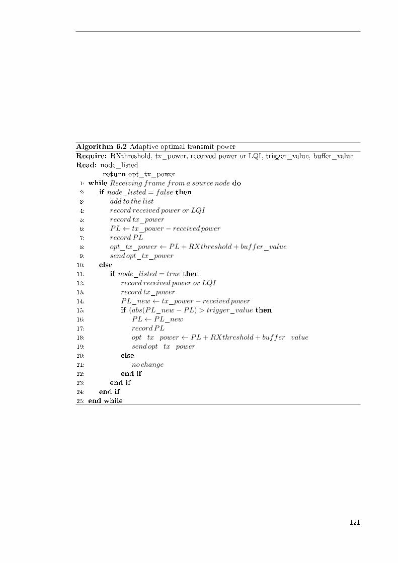
Algorithm 6.2 Adaptive optimal transmit power
Require: RXthreshold, tx_power, received power or LQI, trigger_value, bu�er_valueRead: node_listed
return opt_tx_power1: while Receiving frame from a source node do2: if node_listed = false then3: add to the list4: record received power or LQI5: record tx_power6: PL← tx_power − received power7: record PL8: opt_tx_power ← PL+RXthreshold+ buffer_value9: send opt_tx_power10: else11: if node_listed = true then12: record received power or LQI13: record tx_power14: PL_new ← tx_power − received power15: if (abs(PL_new − PL) > trigger_value then16: PL← PL_new17: recordPL18: opt_tx_power ← PL+RXthreshold+ buffer_value19: send opt_tx_power20: else21: no change22: end if23: end if24: end if25: end while
121
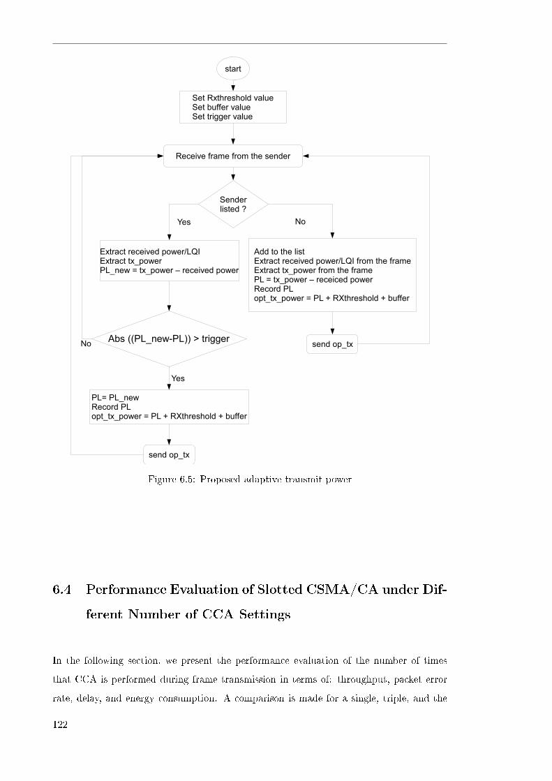
Figure 6.5: Proposed adaptive transmit power
6.4 Performance Evaluation of Slotted CSMA/CA under Dif-
ferent Number of CCA Settings
In the following section, we present the performance evaluation of the number of times
that CCA is performed during frame transmission in terms of: throughput, packet error
rate, delay, and energy consumption. A comparison is made for a single, triple, and the
122

IEEE 802.15.4 standard legacy double CCA; for both hidden and non-hidden node network
scenarios.
6.4.1 Simulation model
Using a Network Simulator (NS-2) [82], we assume an ideal stationary star network topol-
ogy, using the 802.15.4 standard, where the sink node in the middle receives tra�c from
all surrounding nodes, i.e. all nodes are in range of the sink node. For the non-hidden
scenario, all nodes are also in range with one another. For the hidden-node scenario, we
assume that all nodes are in range with one another except for only one pair that cannot
hear each others transmissions. Each node sends data at 40 kbps, i.e. packet interval of
0.02s with 100 bytes packet size, which is less than the channel capacity of 250 kbps. We
increase the tra�c by increasing the number of tra�c connections from the surrounding
nodes to the sink. All sensor nodes are associated to the PAN coordinator before starting
to send packets, and stop before the end of simulation time to allow enough time for pack-
ets sent to be received. Table 6.1 shows our simulation parameters. All simulations were
run independently and their results averaged under di�erent seeds.
6.4.2 Performance metrics at MAC level
The performance metrics analysed in this chapter are as follows:
� Average energy consumption per packet, which is the ratio of the total energy con-
sumed over the number of delivered data packets.
� Throughput and average throughput, which is the fraction of data tra�c correctly
received by the coordinator over a speci�ed period of time.
� Packet Error Rate (PER), which is the percentage delivery ratio, de�ned as the
number of data packets correctly received by the destination node, over the total
number of packets generated by source nodes. This re�ects the degree of reliability
achieved by the network for successful transmissions.
123
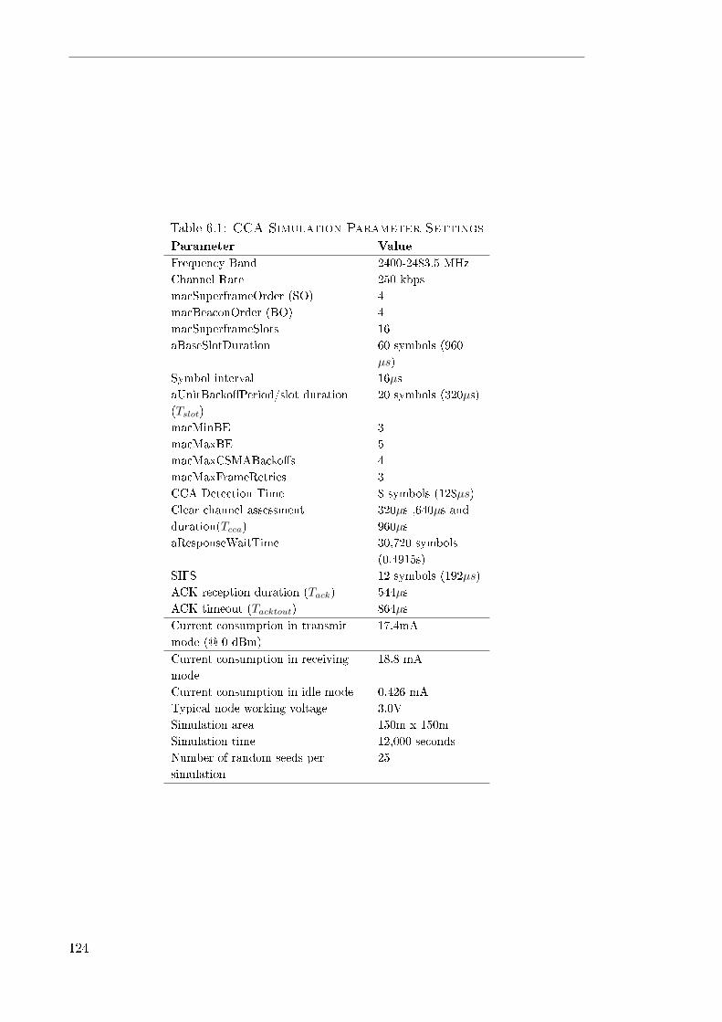
Table 6.1: CCA Simulation Parameter Settings
Parameter Value
Frequency Band 2400-2483.5 MHz
Channel Rate 250 kbps
macSuperframeOrder (SO) 4
macBeaconOrder (BO) 4
macSuperframeSlots 16
aBaseSlotDuration 60 symbols (960
µs)
Symbol interval 16µs
aUnitBacko�Period/slot duration
(Tslot)
20 symbols (320µs)
macMinBE 3
macMaxBE 5
macMaxCSMABacko�s 4
macMaxFrameRetries 3
CCA Detection Time 8 symbols (128µs)
Clear channel assessment
duration(Tcca)
320µs ,640µs and
960µs
aResponseWaitTime 30,720 symbols
(0.4915s)
SIFS 12 symbols (192µs)
ACK reception duration (Tack) 544µs
ACK timeout (Tacktout) 864µs
Current consumption in transmit
mode (@ 0 dBm)
17.4mA
Current consumption in receiving
mode
18.8 mA
Current consumption in idle mode 0.426 mA
Typical node working voltage 3.0V
Simulation area 150m x 150m
Simulation time 12,000 seconds
Number of random seeds per
simulation
25
124

� end-to-end delay, which is the average time taken by a data packet, from the start
of packet generation by the application layer at the source node, to the destination
node (coordinator).
6.5 Results
Figures 6.6, 6.7, and 6.8 show the average energy consumed per packet as the tra�c load
increases when using di�erent number of CCA, for non-hidden nodes, hidden nodes and
both hidden and non-hidden respectively.
�
���
�
���
�
���
�
���
�
���
��� ��� ��� ��� ��� ��� �� ��
����������������� �����������������
�������� ����������
����������
��� ����������������
��� �����������������
��� ����������������
����������
Figure 6.6: Average energy consumption for non-hidden nodes scenario
125

�
�
�
�
�
��
��
��
��
��
��� ��� ��� ��� �� ��� �� ���
����������������� �����������������
�������� ����������
��� ��������������
��� ��������������
��� ��������������
��� ��� ��� ��� �� ��� �� ���
����������
Figure 6.7: Average consumption for hidden nodes scenario
�
�
�
�
�
��
��
��
��
��
��� ��� ��� ��� �� ��� �� ���
����������������� �����������������
�������� �����������
����������
��� �������������
��� �������������
��� �������������
��� ����������������
��� ����������������
��� ����������������
Figure 6.8: Comparison of hidden and non-hidden nodes energy consumption
126
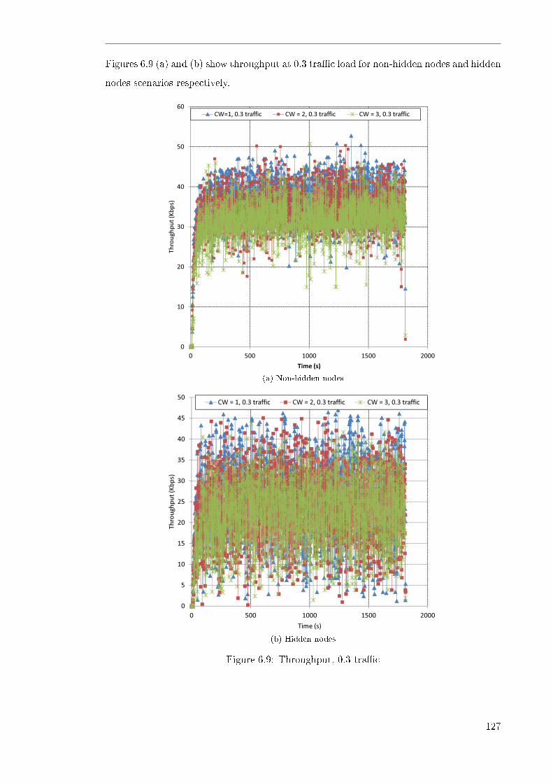
Figures 6.9 (a) and (b) show throughput at 0.3 tra�c load for non-hidden nodes and hidden
nodes scenarios respectively.
��
��
��
��
��
��
������������� �
����� ��������� ������� ��������� ������� ����������
�
� ��� ���� ���� ����
��������
(a) Non-hidden nodes
��
��
��
��
��
��
��
��
��
������������� �
������� ������ ������� ������ ������� ������
�
�
� ��� ���� ���� ����
�������
(b) Hidden nodes
Figure 6.9: Throughput, 0.3 tra�c
127

Figures 6.10, 6.11 and 6.12 shows the average throughput as the tra�c load increases when
using di�erent number of CCA, for (a) non-hidden terminals, (b) hidden terminals, and
(c) both hidden and non-hidden terminals respectively.
�
�
��
��
��
��
��
��
��
���������������� �����
������ ������������
����� ������������
����� ������������
�
��� ��� ��� ��� ��� ��� ��� ���
����������
Figure 6.10: Average throughput for non-hidden nodes
128

�
�
��
��
��
��
��
��
��� ��� ��� ��� ��� ��� �� ��
���������������� �����
��� ��������������
��� ��������������
��� �������������
��� ��� ��� ��� ��� ��� �� ��
����������
Figure 6.11: Average throughput hidden nodes
�
��
��
��
��
��
��
��
��� ��� ��� ��� ��� ��� �� ��
���������������� �����
����������
�� ����������������
�� ����������������
�� ����������������
�� ��������������������
��� ��������������������
��� ���������������������
Figure 6.12: Comparison of hidden and non-hidden nodes average throughput
129
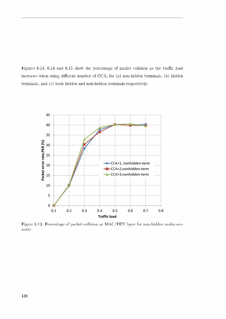
Figures 6.13, 6.14 and 6.15 show the percentage of packet collision as the tra�c load
increases when using di�erent number of CCA, for (a) non-hidden terminals, (b) hidden
terminals, and (c) both hidden and non-hidden terminals respectively.
�
�
��
��
��
��
��
��
��
��
�������������������� ��
������ ������������
����� ������������
����� ������������
�
��� ��� ��� ��� ��� ��� ��� ���
����������
Figure 6.13: Percentage of packet collision at MAC/PHY layer for non-hidden nodes sce-nario
130
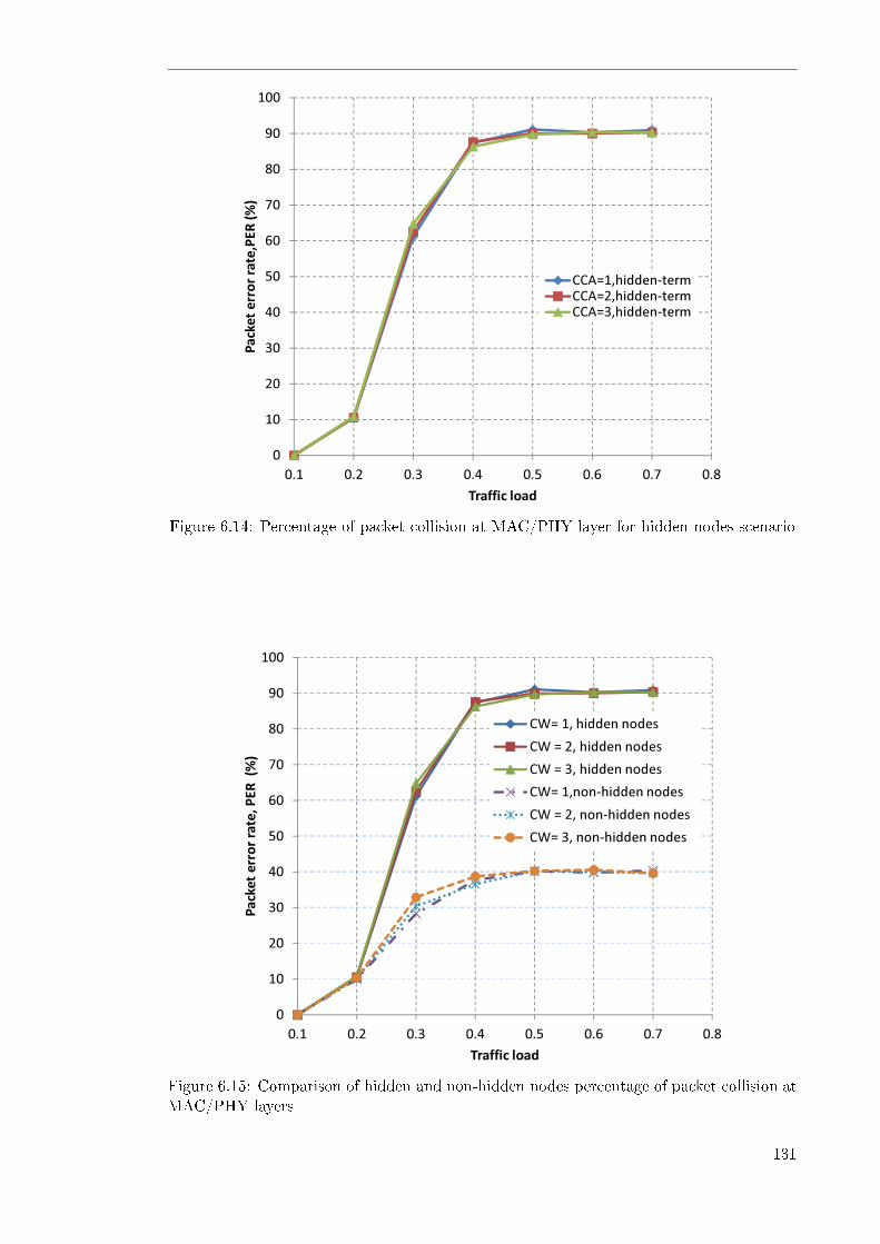
��
��
��
��
��
��
��
�
�
���
�������������������� ��
��� �������������
��� �������������
��� �������������
�
��
��� ��� ��� ��� ��� ��� ��� ��
����������
Figure 6.14: Percentage of packet collision at MAC/PHY layer for hidden nodes scenario
��
��
��
��
��
��
��
�
�
���
���������������������� �
�
�� ���������������������������
��� ��������������������������
��� ���������������������������
�� �����������������������������
��� ����������������������������
�� �������������������������������
�
��� ��� ��� ��� ��� ��� ��� ��
����������
Figure 6.15: Comparison of hidden and non-hidden nodes percentage of packet collision atMAC/PHY layers
131

Figures 6.16, 6.17 and 6.18 show the average packet delay as the tra�c load increases
when using di�erent number of CCAs, for non-hidden terminals, hidden terminals and
both hidden and non-hidden terminals respectively.
��
���
���
���
���
���
���
���
��������������� �������
������� ����������
������� ����������
������� ����������
�
��� ��� ��� ��� ��� ��� ��� ���
����������
Figure 6.16: Average packet delay for non-hidden nodes
132
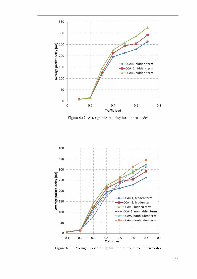
�
��
���
���
���
���
���
���
� ��� ��� ��� ��
��������������� �������
����������
��� �����������
��� �����������
��� �����������
����������
Figure 6.17: Average packet delay for hidden nodes
��
���
���
���
���
���
���
���
���������������� �������
������ ��������
������ ��������
������ ��������
��������� ��������
��������� ��������
��������� ��������
�
��� ��� ��� ��� ��� ��� ��� �������������
Figure 6.18: Average packet delay for hidden and non-hidden nodes
133

6.6 Discussion
The 802.15.4 CSMA/CA MAC is prone to two types of collisions, collisions caused by
hidden node phenomenon, and collisions caused by the selection of the same backo� slot
with another node. In CAP neither of these collision can be avoided by the standard. This
reduces the reliability of IEEE 802.15.4 even for the case of a lightly load WPAN.
While we can conclusively say that there is some improvement in terms of: 1) throughput;
and 2) average packet delay, when sensing the channel for shorter duration (once), instead
of twice or thrice as the tra�c load increases; there is no signi�cant di�erence in terms of
energy consumption and packet error rate. This can be explained in terms of probability as
described in chapter 7, section 7.2.2. The likelihood of a channel being idle/busy the second
or third time is smaller once it has been sensed busy/idle the �rst time. The reason for
employing the standard default value when consecutively checking the channel, is to avoid
packets colliding with an acknowledgment frame; which is possible (with small probability)
when packet size is big, i.e. taking longer to transmit. However for small packet size, even
checking the channel only once does not appear to cause a problem. Furthermore, in the
case of non-hidden terminals; e�ective collision resolution is achieved by adjusting the
backo� exponent (BE), based on consecutive clear channel assessment (CCA) busy/idle
results, and therefore CCA has a small part to play. In case of hidden nodes, the standard
does not tackle the collision problem, and therefore network performance in terms of:
energy consumption, throughput, packet error rate, and delay degrades tremendously.
The proposed design will be e�ective for low data tra�c WSN applications, for high tra�c
applications, tra�c scheduling will be a more appropriate choice.
6.7 Conclusion
In this chapter, we presented an investigation aimed at determining the impact of the
number of times the CCA is performed in the 802.15.4 MAC during frame transmission
in terms of: throughput, packet error rate, delay, and energy consumption. Both hidden
and non-hidden nodes in a network system are considered. Results indicated a serious
134

degradation in network performance, even for a small number of hidden nodes in a network.
Following these results, a proposed cross layer (PHY-MAC) mechanism to save energy,
reduce interference, improve scalability and reliability, and reduce packet collisions due to
hidden terminals has been presented. The proposed design uses a new algorithm to increase
the sensing coverage area, and therefore greatly reduces the chance of packet collisions due
to hidden nodes. Moreover, the design uses a new dynamic transmission power control
(TPC) to further reduce energy consumption and interference. The proposed changes can
be easily integrated, with minimal or no disruption into the legacy 802.15.4 CSMA/CA
design.
135

136

Chapter 7
Analysis of Slotted CSMA/CA Using Markov Chain
The design and performance evaluation of MAC protocol can be carried out
using several approaches, including simulation, hardware platform, theoreti-
cal mathematical model, or a combination of such approaches. This chapter
contains a proposed model to capture essential features of the IEEE 802.15.4
slotted CSMA/CA by using the Discrete Markov chain. Accurately modelling
the CSMA/CA will result in better performance predictions for parameters,
such as throughput, delay, and energy consumption. Moreover, it will o�er
deeper insights into the strengths and weaknesses of the multiple access con-
trol operation as well as possible enhancement opportunities. Previous studies
[70, 111, 102, 109, 112, 103, 104, 113, 105] have, to a certain extent, provided
an inspiration in developing the current proposed model.
7.1 Introduction
In analytical mathematical modelling, one relies on the assumptions and approximations
made to simplify mathematical expressions while closely modeling/describing an original
protocol or process. In Bianchi's [111, 70] approach, a Markov chain is proposed to model
the IEEE 802.11 Distributed Coordination Function (DCF) while the packet transmission
probability is computed given the network con�guration and contention window size. Note
that in IEEE 802.15.4 the DCF is known as the Contention Access Period (CAP).
Bianchi [70, 111] presented a Markov chain model describing the performance of 802.11
DCF using the probability that a device is in the channel-accessing state, using the key
137

approximation that each transmission attempts, regardless of the retransmission experi-
enced; thus, all packets collide with a constant and independent probability. In light of the
802.11, when using this model, it is possible to compute the probability that a given station
attempts transmission in a given time slot. The transmission probability can then be used
to obtain the probability of an idle, successful, and collision slot for a number of contending
stations. However, in 802.15.4, it is not appropriate to use this key approximation because
the channel sensing is performed according to the value of CW before entering the trans-
mission state. Markov chain modelling for 802.15.4 di�ers from 802.11 CSMA/CA DCF
because, in 802.11, nodes continuously monitor the channel and are therefore continuously
aware of the channel state [103]. In the 802.15.4 standard, a node does not listen to the
channel continuously; thus, it is possible to switch to low-power mode during a random
back-o� delay to save some energy. Only after such a random delay does the contending
node wake up to listen to the channel for CW back-o� slots. Therefore power consumption
during channel listening is minimised.
Ziouva and Antomakopolas [114] modelled 802.11 DCF assuming that the channel access
probability and station collision probability are independent of channel status. Chuan [115]
corrected the model presented in [114] using Bianchi's improved model by considering the
busy medium condition.
Currently, the literature on the IEEE 802.15.4 analytical evaluation models is insu�cient.
Most of the existing literature has drawn considerable inspiration from Bianchi's work
[111, 70] on the modelling of 802.11 MAC DCF.
Park [102] proposed a new 802.15.4 Markov chain model in saturation conditions using
the probability of a device in the channel-sensing states (CCAs) instead of the channel-
accessing states, relying on the same assumptions as in [70]. The key approximation is the
busy probability of the channel at the �rst and second CCA regardless of the stages.
In [109], the Markov chain model was derived by considering which embedded points were
correct after the completion of a frame transmission of any device, regardless of success or
failure, which is also di�erent from the conventional 802.11 model [70, 111].
Pollin [103] assumed that each device carrier sensing probability, rather than its packet
sending probability, was independent.
One of the di�culties in analysing the 802.15.4 CSMA/CA in CAP lies in modelling its
exponential backo� behaviour. Apart from di�erent approaches, the main parameter that
138

brings di�erent results is that of �nding the probability of a node to be on the �rst CCA
as well as assumptions made that lead to di�erent results.
The scope of this chapter lies in the construction of a mathematical model based on the
discrete Markov chain in describing the performance of slotted 802.15.4 CSMA/CA during
CAP. The relationship among the successful transmission probability, throughput, and
average energy consumption was derived. The model is more accurate, is simple, and has
recti�ed some of the minor issues that emerged in previous work, such as:
� The time used to calculate CCA energy consumption (equation 14) in [116] is incor-
rect; the authors utilised the time used to send the packet (i.e., payload divided by
data rate) instead of the appropriate time spent to perform CCA.
� The transition matrix, equation 4 in [117, 103], is incorrect as, once the node �nds
the channel busy in the �rst CCA, it will move straight to the next stage and not
perform the second CCA. Similarly, equation 3 in [108] de�nes the probability of
a channel being idle if it was busy in the previous slot; however, according to the
standard, once the channel is found to be busy, the algorithm moves to the next
stage (increases BE and NB).
� The backo� time is included in both the time to successfully receive a packet and
collision time as this is part of the time spent to transmit a packet (equation 7.12
and 7.13).
Discrete Markov Chain De�nition
De�nition 1.A discrete Markov process {Xn} is a stochastic process with the property
that the probability of any particular future behaviour of the process, when the current
state is known exactly, is not altered by additional knowledge concerning its past behaviour.
From the de�nition {Xn} is Markov chain if
Pr {Xn+1 = j | X0 = io, ....Xn−1 = in−1, Xn = i} = Pr {Xn+1 | X = i}
For all time points n and all states i0.......in−1, i, j.
Notation : Pr {Xn+1 = j | Xn = i} = Pij , where
139

Pij ≥ 0 for i, j= 0,1,2.... and∑∞
j=0 Pij = 1 for i = 0, 1, 2, 3, ...
Once all the transition probabilities have been obtained, the Markov chain can be numer-
ically solved to obtain the stationary probability distribution of each state using recursive
solution, π = πA, where A is the initial state condition and πis the transition matrix.
7.2 Performance Modeling and System Description
This section presents the proposed two-dimensional discrete time Markov chain model to
analyse throughput, reliability and energy consumption of the slotted CSMA/CA. For a
complete slotted CSMA/CA algorithm, refer to chapter 6, section 6.2.1.
Consider a star network topology with a group of WPAN devices that use slotted CS-
MA/CA with an optional acknowledgment (ACK) in sharing a radio channel when trans-
mitting to the PAN coordinator. The standard speci�es that all nodes ensure that any
transmission initiated should be complete before the end of the beacon interval. Therefore
the probabilities of channel access and success transmission are evaluated as a function of
time, starting from the reception of the beacon sent by the coordinator, until the end of
the superframe.
Generally, a node accessing the channel during the CAP portion of the superframe can be
in one of the �ve states, which include:
� backo�
� carrier sensing
� transmit
� collision
� idle
7.2.1 Model assumptions and mathematical modeling
The following are the assumptions made in the proposed model:
140
� The network consists of �nite number of N contending nodes associated with a com-
mon coordinator in a one hope star topology.
� All nodes are perfectly synchronised at backo� period boundaries, and the inactive
period does not exist (i.e., BO=SO).
� An ideal channel condition, where all nodes are within the carrier sense range of each
other (i.e., no hidden nodes).
� Each node always has a packet available for transmission, which implies operating in
a saturation condition.
� Using �xed size data packets of the L-backo� slot duration.
� The probability to start sensing the channel is constant and independent of all other
nodes and independent of the retransmission this packet has su�ered in the past.
This is the main approximation assumption, which is di�erent from Bianchi's [111],
where the packet sending probability is assumed to be independent.
Let s(t) be the stochastic processes representing the backo� stage (0...m) for a given node
at time t, where m is the maximum backo� stage (NBmax), and let b(t) be the stochastic
process representing backo� time counter for a given node at time t. The time t corresponds
to slot time and is related to system time. Table 7.1shows di�erent symbols and parameters
used in the current model.
Note that b(t) and s(t) are time discrete stochastic processes in a chain; however, b(t)
is not memory less (not Markovian) as its value depends on the history (e.g., how many
times the node has tried to access the channel with or without success and the number of
retransmission). However for convenience:
Let bij =lim
t→∞Pr {s(t) = i, b(t) = j} i = ε(0.m)
is the steady state probability of any state. Then the random process of the backo� stage
s(t) and the backo� counter b(t) constitute a two dimensional Markov chain X(t) = {(s(t),
b(t))}
The delay window Wi is initially W0 = 2MacMinBE , a device with a pending frame for
transmission, will select a random backo� counter value between [0,W0 − 1]and doubled
at every stage until Wi = Wmax = 2macMaxBE . Therefore, the size of the backo� window
at the backo� stage s(t) = iε {0...m} is Wi = 2min(MacMinBE+i,macMaxBE).
141

Figure 7.1: Markov chain states for single CCA
Figure 7.2: Markov chain states for double CCA
142

7.2.1.1 State Transition Probabilities
The total number of states is higher than �ve, as illustrated in Figure 7.2. Using the proba-
bilities de�ned in table 7.1 and the identi�ed assumptions, the state transition probabilities
associated with the Markov chain are a two-dimension Markov chain with the following
transition probabilities:
P (i, j | i, j + 1) = bi,j|i,j+1 = 1 i = ε [0,m] j = ε [0,Wi − 2]
P {i,−1 | i, 0} = bi,−1|i,0 = (1− α) i = ε[0,m]
P {i, j | i− 1, 0} = α/Wi
P {i, j | i− 1,−1} = β/Wi
P {0, j | m, 0} = α/W0
P {0, j | m,−1} = 1/W0 j = ε [0,W0 − 1]
P {0, j | i,−1} = b0,j|i,−1 = (1− β)/W0 i = ε[0,m− 1] j = ε [0,W0 − 1]
(7.1)
Equation 1 of the transition probability is the condition to the decrement of the delay
back-o� counter, regardless of whether the channel is idle or not.
Equation 2 is the condition for performing the second CCA given during the �rst CCA
when the channel was idle.
Equations 3 and 4 show the move to the next stage whereby the back-o� exponential (BE)
is increased because of the busy channel at the �rst or second CCA, respectively.
Equations 5 and 6 are the condition when the maximum stage is reached and, as a result,
the packet is dropped and the transmission process starts again in the �rst stage.
Equation 7 is the case of the packet being transmitted after the channel is found to be idle
in the �rst and the second CCA.
From expression 7.1 , we have
bi,j =Wi − jWi
bi,0 (7.2)
143

Table 7.1: Di�erent symbols and parameter used for the model
τ The probability that a node attempts a �rstcarrier sensing to transmit a frame
α The probability that a node �nds the channelbusy during the �rst CCA
β The probability that a node �nds the channelbusy during the second CCA
Ptx Probability that at least one node istransmitting in any given time slot
Ps Probability that at least one node istransmitting successfully in any given time
slot
pc Collision probability
Pidle Probability that the node is idle
ACK+PHR+SHR, TACK 11 bytes = 352µs
tack 12 PHY symbols = 192µs
σ a unit backo� slot duration
7.2.2 Probability of transmitting
Before transmitting a packet, each contending node performs the back-o� algorithm, where
each node is randomly delayed by extracting an integer from a uniformly distribution
between 0 and Wo-1; before sensing the channel a node enters, with the probability 1/Wo,
one of the states is {0,j,w-1} with j E [0,Wo-1]. If there is no random delay j= 0, then the
node enters the �rst carrier sensing straight away.
After the random delay, in order for a node to transmit a packet, it �rst performs a
predetermined number of CCAs to determine if the channel is idle in all CCAs performed
(in this case, CW=2 or 1). After sensing the channel to be free, the node immediately
enters the transmission state. At this stage, the packet transmission duration in slots, L,
is included, followed by a sequence of idle slots until the end of the superframe duration.
The focus is on �nding the probability that the node is in the sensing state, which can be
determined using the state transition diagram (Figure 7.2 or 7.1) and the transition matrix
that describe all possible nodes' states. The probability of transmitting Ptx will depend on
the probability of being in a sensing state and the probability of �nding the channel idle
during CCA.
When a node attempts to send a frame, its backo� counter has reached zero and it is
144

no longer idle as it has a frame to send. Here we consider τ , instead of the product of
(1− Pidle) τ as at this stage Pidle = 0. τ is di�erent from that of 802.11 in [70], whereby
the node is always listening to the channel when not transmitting. Therefore, we do not
model the transmission state, but focus on the probability that a device is in the sensing
states. In the case of 802.15.4, τ is a function of exponential delay line, as explained in the
previous section 7.2.1.1.
The probability that a node starts to transmit is
Ptx = τ(1− α)(1− β) (7.3)
Which requires the node to be sensing with the probability τ , and the channel to be idle
during the two CCAs, with the probability (1− α)(1− β). We de�ne τ , as the conditional
probability that a device is at one of the �rst CCA states bi,0, out of the backo� states as
follows:
τ =∑mi=0 bi,0∑m
i=0
∑Wi−1j=0 bi,j
= 2(1−(α+β−αβ)m+1∑mi=0(W02min(i,BEmax−BEmin)+1)(α+β−αβ)i
(7.4)
since the Markov chain normalised condition
∑i
∑j
bi,j = 1 (7.5)
Now we need to �nd the remaining two unknowns, α and β. Let TL and TACK denote
time duration in the number of slots for transmitting an L-slot frame and receiving ACK
frame, respectively. Similar to [117], the probability α, the probability that a node �nds
the channel occupied either due to data transmission or ACK transmission in the �rst CCA
can be estimated as follows:
α = αL + αack (7.6)
where αL is probability of �nding the channel busy during the �rst CCA due to data
transmission, which is:
145

αL = L[1− (1− τ)N−1
](1− α) (1− β) (7.7)
and αack is probability of �nding the channel busy during the �rst CCA due to ACK
transmission, equal to:
αack = LackNτ (1− τ)N−1
1− (1− τ)N(1− (1− τ)N−1
)(1− α) (1− β) (7.8)
Finally, the probability of �nding the channel occupied during the second CCA is not
independent like the �rst CCA, it depends on the probability of �nding the channel idle
during the �rst carrier sense, which is:
β =1− (1− τ)N−1 +Nτ (1− τ)N−1
2− (1− τ)N +Nτ (1− τ)N−1(7.9)
The expression for the sensing probability τ and the busy channel probabilities α and β
form a system of non-linear equations that can be solved through numerical method. To
evaluate other target probabilities, we model how the number of nodes contending to the
channel varies with time.
7.2.3 Probability of successful transmission
The probability that a node transmit successfully (Ps = 1−Pc), Ps is the probability that
a node start sensing alone and �nds the channel idle for predetermined CCA slots (i.e.,
the probability that exactly one node transmit on the channel), given by:
Ps = τ (1− τ)N−1 (1− α) (1− β) = Ptx(1− τ)N−1 (7.10)
A transmission is considered a successful one if an acknowledgment frame is received in
time (before ACK timeout). The frame transmission starts from the time a node perform
random backo� to the time an ACK frame is received, including an Inter-Frame Space
(IFS) time after ACK frame transmission.
146
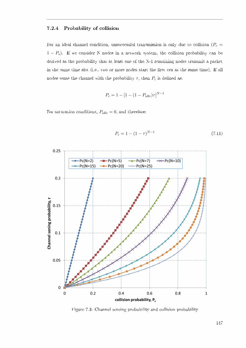
7.2.4 Probability of collision
For an ideal channel condition, unsuccessful transmission is only due to collision (Pc =
1 − Ps). If we consider N nodes in a network system, the collision probability can be
derived as the probability that at least one of the N-1 remaining nodes transmit a packet
in the same time slot (i.e., two or more nodes start the �rst cca at the same time). If all
nodes sense the channel with the probability τ , then Pc is de�ned as:
Pc = 1− [1− (1− Pidle)τ ]N−1
For saturation conditions, Pidle = 0, and therefore:
Pc = 1− (1− τ)N−1 (7.11)
����
���
����
���
����
��������������� ���������
����� ����� ����� ������
������ ������ ������
�
� ��� �� ��� ��� �
����������������� ����Figure 7.3: Channel sensing probability and collision probability
147

Figure 7.3 shows the relationship between sensing probability and collision probability as
the number of contending nodes increases.
7.3 Transmission and Collision Timings
In this model, for accuracy, the average backo� period and interframe space (LIS/SIF) are
considered as part of the time to successfully transmit a frame. This is contrary to previous
models derived in [113, 118, 111, 70, 109]. The total number of time slots required for a
single successful transmission is:
Ts = E[Backoff period] + no. of cca× TCCA + L+ LACK + tack + TIFS (7.12)
where TCCA, TL, tack, and LACK are time duration in number of slots for performing a
CCA, transmitting data frame, waiting for an acknowledgment frame and receiving an
ACK frame respectively. E[Backoff period] is the average backo� period in terms slots
as shown in the Table 7.2. no. of cca is the number of times CCA is performed (default
2), and TIFS is the Inter-Frame Spacing, depending on the size of the data frame, either
Short Inter-Frame (SIF) or long (LIF) is used (Figure 7.4).
Similarly, the total number of time slots for a single collision transmission is
Tc = E[Backoff period] + no. of cca× TCCA + L+ Tack,tout (7.13)
where Tack,tout is ACK timeout of ACK [7]. In 802.15.4 ACK waiting duration is speci�ed
by macAckWaitDuration (2.7 slots in 2.4 GHz channel).
148
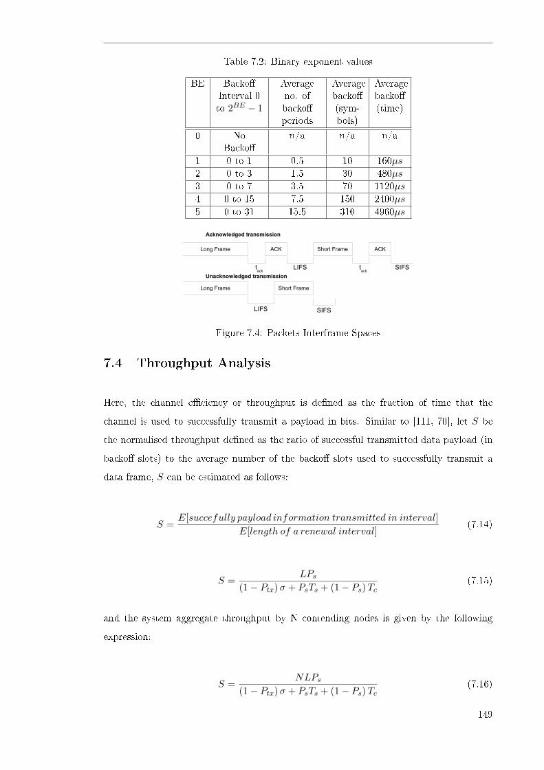
Table 7.2: Binary exponent values
BE Backo�Interval 0to 2BE − 1
Averageno. ofbacko�periods
Averagebacko�(sym-bols)
Averagebacko�(time)
0 NoBacko�
n/a n/a n/a
1 0 to 1 0.5 10 160µs
2 0 to 3 1.5 30 480µs
3 0 to 7 3.5 70 1120µs
4 0 to 15 7.5 150 2400µs
5 0 to 31 15.5 310 4960µs
Figure 7.4: Packets Interframe Spaces
7.4 Throughput Analysis
Here, the channel e�ciency or throughput is de�ned as the fraction of time that the
channel is used to successfully transmit a payload in bits. Similar to [111, 70], let S be
the normalised throughput de�ned as the ratio of successful transmitted data payload (in
backo� slots) to the average number of the backo� slots used to successfully transmit a
data frame, S can be estimated as follows:
S =E[succefully payload information transmitted in interval]
E[length of a renewal interval](7.14)
S =LPs
(1− Ptx)σ + PsTs + (1− Ps)Tc(7.15)
and the system aggregate throughput by N contending nodes is given by the following
expression:
S =NLPs
(1− Ptx)σ + PsTs + (1− Ps)Tc(7.16)
149

where Ts is the average time the channel is sensed busy due to successful transmission
(equation 7.12), Tc is the average time the channel is sensed busy by each node during a
collision (equation 7.13), and σ is the duration of an empty slot. To convert equation 7.15
and 7.16 to bit per second (bps), multiply by a normalised constant, C = 80bits0.32ms for the
802.15.4 2.4GHz band, 250kbps data rate.
7.5 Average Energy Consumption Analysis
In order to determine the average energy consumed by a node, we have to determine
the average time (probability) the node occupies each state (i.e., transmit, receive, idle,
sleep, CCA and collision) and multiply by each state associated power expenditures. The
transmit power PTX , receive and sensing power PRX and idle power PIDLE can be readily
obtained from the node's data sheet such as the one in chapter 2, Table 2.2. In the
saturated condition, nodes always have a data frame to transmit; thus, PIDLE is the power
used when the node is in the exponential delay time (backo�) and for the remaining slots
after the frame transmission between the two consecutive transmissions. Note that the
power consumed while receiving and performing CCA is larger than the transmit power
consumption [103, 119]. Furthermore, in the current model the sleeping power PSLEEP ≈ 0,
because superframe BO= SO.
To �nd the individual state energy consumption, simply use the appropriate state prob-
ability and multiply with associated power consumption. Here, the interest is in �nding
the average energy consumption for packet transmission including both successful trans-
mission and packet collision. Using equations 7.3, 7.10 and 7.11, the average energy for
packet transmission is given by
E = τ (1− α) (1− β) [(1− Ptx)PIDLE + LPTX + LACK (PsPRX + PcPIDLE)] (7.17)
7.6 Discussion
In wireless sensor networks, it is important to minimize energy consumption, maximise the
number of successful transmissions (reliability), and minimise the probability of collisions.
150

The duration of collision is as long as the length of the packet involved in the collision;
it is therefore essential to reduce the number of collisions to improve network reliability,
energy consumption and throughput.
In CSMA/CA, as the number of nodes increases, the chances that two or more nodes
transmit on the same slot increase, which subsequently increases the chance of transmission
loss due to the increased number of collisions. In addition, the probability of �nding the
channel idle in the sensing slots decreases when the number of nodes, N, increases as a
large part of time is spent in the back-o�; thus, the network throughput will downgrade
with the signi�cant increase in the frame service time.
Binary exponent, BE, is the main parameter for avoiding collision; basically, the contention
window adapts to the high value by increasing BE when the active population of nodes
is large. This reaction reduces the load on the network and should decrease the collision
probability. The MAC latency is high if the contention window is large. The issue is
when a station successfully transmits as it resets the contention window to a small, �xed
minimum value of W0. Consequently, the node has to rediscover the correct contention
window size, thereby wasting bandwidth. The 802.15.4 standard BE back-o� does not
assume the advantage of shared learning when the number of nodes increases or decreases.
Although BE back-o� improves fairness because after completion of each successful packet
transmission, a node needs to wait for a random back-o� time, which can help other nodes
seize the channel. A technique such as IEEE 802.11e can be used to dynamically tune
the value of BEmin and BEmax to adapt to the number of contending nodes. Obviously,
small contention windows are desirable when the number of contending stations is low to
keep the number of empty unused slots relatively low. However, an empty slot is much
more desirable than collision as the duration of an empty slot is comparatively smaller
than collision duration. A larger contention window o�ers better performance because it
reduces the collision probability.
The waste of channel utilisation is the other factor in slotted CSMA. When the remaining
number of back-o� periods in CAP are not enough to process the transmission of a data
frame, the channel will remain idle because the sensor node waits for the next superframe.
Obviously, the number of remaining back-o� periods will depend on the length of the
superframe BO or beacon interval, the size of the data payload and the number of CCA
performed. To increase channel utilization, a fragmentation scheme can perhaps be used
to divide the data frame to �t into the remaining number of back-o� slots in a superframe
151

CAP.
To get a more accurate analytical model result, future models need to include the real
operation value of a superframe SO and BO, which determines the total number of slots
in CAP. The CAP slots specify the number of available slots for packet transmission and
therefore can impact the probability that there are not enough slots left in the current CAP
for transmission and the overall performance in general. For example when SO=BO=3,
the number of CAP slots, CAPslots =16∗60∗23symbols
20 symbols = 384. Although the proposed model
remains to be validated using simulation or hardware tools, some of the �ndings in chapter
6, section 6.5 on the probability of collision when using single CCA or double CCA re�ect
the proposed model probability of �nding the channel busy in the second CCA, which
is much smaller as given in equation 7.9. These results demonstrate that changing the
default CW from 2 to 1 can bring bene�ts in terms of throughput. However, performing
the second CCA does not show signi�cant improvement in terms of collisions.
7.7 Conclusion
In this chapter, a more accurate model has been proposed based on discrete Markov chain
describing the performance of slotted 802.15.4 CSMA/CA during CAP. The relationships
among the successful transmission probability, throughput and average energy consumption
are derived. Some of the minor issues apparent in previous studies have been recti�ed while
maintaining the model's simplicity. Future work and some of the 802.15.4 CSMA/CA CAP
issues have been thoroughly discussed.
152

Chapter 8
Conclusions and Future Work
This chapter contains a summary of contributions of this thesis and some of
future research directions in wireless sensor networks.
8.1 Concluding Remarks
The emerging �eld of WSN research combines numerous disciplines and addresses a com-
bination of the major challenges in sensor techniques, embedded techniques, distributed
information processing, and wireless communication. WSNs is a burgeoning area of re-
search with many challenges, including managing energy consumption and network con-
nectivity. While the wireless channel has enabled cheap establishment and maintenance
costs of WSNs, it adds constraints that are not found in wired networks. Specially, limited
bandwidth, channel errors, and nodes that have limited operating energy.
Developing new WSN applications with severe resource constraints will require innovative
solutions to overcome the above issues as well as improving the robustness of network
components, and developing sustainable and cost e�ective implementation models. New
developed WSN protocols/algorithms and components will have to further improve energy
e�ciency, bandwidth e�ciency and connectivity.
The IEEE 802.15 standard was designed for low rate wireless personal area networks (LR-
WPANs), making it the �rst WSN enabling standard. However, the development of a
particular WSN application will require a high degree of integrated solution to achieve
desirable and e�ective communication. This requires both robust hardware and e�cient
protocols/software solutions. So far there has been no clear guidelines or design rules that
153
have been followed in designing sensor network architectures because of the wide range of
sensor applications, with each application having its own unique purpose and performance
requirements (i.e, various hardware and network capability). Similarly, the general IEEE
802.15.4 standard and the likes have been implemented for a broad range of wireless PAN
applications and therefore not optimised for a speci�c application.
The main aim of this thesis has been to investigate techniques for improving the perfor-
mance of WSNs to maintain reliable network connectivity, scalability and energy e�ciency.
Results and the overall work presented in this thesis form a part of an emerging WSN
research and establish contribution in achieving more e�cient WSNs and applications.
Speci�cally, the following areas have been examined in detail: WSN transmission power
control, self-con�guration, MAC design in the presence of hidden nodes and CSMA/CA
analytical modeling.
The study sought answers to the following questions which are addressed in four areas of
study (Section 3.3):
1. How can we speci�cally test multi-hop TPC communication versus single-hop com-
munication using typical wireless sensor node hardware parameters?
2. What is the performance advantage of using multi-hop TPC in energy constraint
WSNs instead of a single-hop in terms of energy e�ciency and other important
performance parameters?
3. What is the impact of beacon interval (BI) and number of nodes during WSN associa-
tion and synchronization stages in terms of energy and association or synchronization
time?
4. How can we improve the performance of WSNs during association and synchroniza-
tion stage (self-con�guration)?
5. What is the impact of the number of times the clear channel assessment (CCA) is
performed in the 802.15.4 MAC during frame transmission in terms of throughput,
packet error rate, delay and energy consumption for both hidden and non-hidden
nodes in a network ?
6. What can be done to improve the performance of the 802.15.4 MAC during frame
transmission stage?
154

7. How can Markov chains be used to accurately model the IEEE 802.15.4 slotted
CSMA/CA ?
8. What is the relationship between di�erent performance variables and the MAC pa-
rameters derived from the Markov Chains?
The following section highlights the major contributions of this thesis.
8.2 Main Research Contributions
The main contributions of this thesis are summarised as follows:
� The transmission power control (TPC) was investigated in multi and single-hop
WSNs using typical hardware platform parameters via simulation and numerical
analysis. A novel approach to testing TPC at the physical layer was developed, and
results have shown that contrary to what has been reported from previous studies,
in multi-hop networks TPC did not save energy. Both the radiation and electronic
components of the energy consumption were investigated, and results indicated that
sending packets using a short-range multi-hop path, instead of a single-hop, does not
necessarily save energy as suggested by some researchers. Moreover, transmitting in
single-hop networks at lower transmission power levels, while still maintaining reli-
able connectivity, reduced energy consumption by up to 23%. Furthermore, we have
shown that both packet collisions and delays a�ect the performance of WSNs that
have an increased number of hops. Since the use of TPC in star topology/cellular
networks transmission can save energy, we have recommended cluster based (hybrid)
or similar topology over completely multi-hop topology. Relationship among protocol
layers was also revealed; possible improvement suggested; insight when developing
wireless sensor networks protocol and the signi�cance of TPC;
� The performance evaluation of the 802.15.4 MAC during device association and syn-
chronization with the PAN coordinator, showing the impact of beacon interval and
the number of associating nodes in terms of association time delay and energy con-
sumption in stationary wireless sensor networks has been investigated. Results il-
lustrated that energy consumption and association time increased with increasing
number of nodes associating with a coordinator. Moreover, short beacon intervals
155

consumed more energy due to the frequency of beacon frames that nodes have to
keep track of to maintain synchronization. However, short beacon intervals reduced
the time required for the nodes to associate, in contrast to longer beacon intervals
that are undesirable for real time and mobile applications. Furthermore, for longer
beacon intervals, BO= 12 to BO=14, it has been shown that there was an abrupt
increase in energy consumption as the number of associating nodes increased, even
for as few as as four nodes. This appeared to be the �rst investigation of the perfor-
mance of the 802.15.4 MAC beacon interval setting and the number of associating
nodes. To conserve energy in WSNs, we expect to use longer beacon interval (BI)
and shorter active periods (SD) so that the nodes can go into inactive/sleep state
during CAP to save energy. To date the longest beacon interval is 251.66s (about 4
minutes). Our results demonstrated that even with 7 nodes connected to the PAN
coordinator, the association delay and energy consumption due to synchronization,
increased. The question was whether the association energy consumption will out-
weigh the bene�t of duty cycle power management for larger beacon intervals, as the
number of associating nodes increases.
� A study to determine the impact of the number of times the CCA was performed in
the 802.15.4 MAC during frame transmission in terms of throughput, packet error
rate, delay and energy consumption has been presented. Both hidden and non-hidden
nodes in a network system were considered. Results indicated a serious network
performance degradation even for a small number of hidden nodes in a network.
Following these results a proposed cross layer (PHY-MAC) mechanism to save energy,
reduce interference, improve scalability and reliability, and reduce packet collisions
due to hidden terminals has been presented.
� Finally, an improved two dimensional discrete time Markov chain has been proposed
to capture essential features of the IEEE 802.15.4 slotted CSMA/CA. This model has
recti�ed some of the issues apparent in previous studies. Important relationship for
the successful transmission probability, throughput and average energy consumption
have been derived. Moreover, the proposed model provided greater insight into the
strengths and weaknesses of the MAC operation, and future possible enhancement
opportunities.
156

8.3 Future Work
WSNs have a promising future, but additional research is needed so that the remaining
challenges can be addressed. Future WSNs will still be constrained by modest power
supplies provided by both passive (e.g., solar and vibration) and active (e.g., battery
power and external power source) sources of energy. Thus, energy e�ciency and reliable
connectivity will continue to receive signi�cant attention in the research and design of
WSNs. We believe that such research will contribute to the development of a new, inclusive
paradigm within the �eld of wireless communications. Following the current research, a
starting point for this work will be the inclusion of additional cross-layer designs at multiple
layers of the communication protocol stack due to the interdependence that exists among
all of the layers. This has to be explicitly considered when designing communication
protocols aimed at quality of service (QoS) provisioning on resource-constrained WSNs.
In the current research, the work is limited to the PHY-MAC cross-layer.
There is also a need to use suitable hardware platforms in the experimentation and im-
plementation phases of this work. This is important because the optimal choices of sensor
system, processor, wireless interface, and memory technology are application dependent
and exhibit temporal dependence for a given application. The concept is to get all the
bits right across layers, hardware, and algorithms/software. Also, it is important for the
newly-designed protocols to relate e�ectively to available hardware as opposed to sounding
good on paper while failing the test of successful implementation with current or future
technologies. Future work will validate the proposed CSMA/CA Markov chain model using
a simulator or hardware platforms.
Most of the existing research in the �eld has been restricted to the star topology, in which
devices in a PAN can always reach the coordinator in one-hop distance; however, for a large
WSN, not all devices will be able to communicate with the coordinator directly; rather, they
must communicate through intermediate devices (routers) to forward messages. There is
a need to consider di�erent application scenarios and to incorporate harsh environmental
conditions in future studies. For example, reasonable designs must include appropriate
considerations of conditions that wireless channels are likely to encounter, such as noise,
interference, and other environmental factors, such as temperature, humidity, and wind.
Furthermore, since sensor networks will become a seamless part of larger networks, so
additional investigations should be conducted focusing on the combination of WSNs with
157
existing and future technologies, such as the Internet and GPSs.
The investigations and design development in this research considered homogeneous sensor
networks. However, there are important WSN applications in which this is not the case.
Future studies should include heterogeneous sensor networks that consist of several nodes
with extra capability in a network.
There is also a need for further investigation to determine possible approaches that would
improve the performance of 802.15.4 during the PAN association and synchronization
stages. This research raised important issues during network self-con�guration. Future
studies should consider improvements in self-con�guration designs. For example, such
studies could evaluate the implementation of an adaptable beacon interval to make use
of both short intervals for a quick association time and suitable large beacon intervals for
saving energy. The coordinator could start with a short beacon interval repetitively to
allow nodes to quickly associate with the coordinator; then, after a predetermined period
of time, the coordinator could switch to a large beacon interval to save energy. Subse-
quently, the coordinator could switch again to a short beacon interval to allow new nodes
to associate and disassociated nodes to re-associate.
Work also is needed to improve the 802.15.4 standard BE backo�, which does not take
the advantage of shared learning when the number of nodes increases or decreases. For
example, a technique such as the one in the IEEE 802.11e standard could be used to
tune the value of BEmin and BEmax dynamically to adapt to the number of contending
nodes. A fragmentation scheme also can be used to divide the data frame to �t into the
remaining number of backo� slots during the contention access period (CAP) to increase
channel utilization. While protocols that are implemented for speci�c wireless applications
can be advantageous in the future, �exibility is vitally important in future applications in
which sensors will be able to adapt to changing objectives and to evolving applications.
Future studies should focus on determining the appropriate balance between a protocol's
adaptability, complexity, and performance in WSNs.
Finally, while energy considerations have dominated most research related to WSNs, one
of the technology trends is towards increasingly higher bandwidth. This emphasis has
resulted from the increasing interest in real-time applications that involve imaging and
video sensors, which pose additional challenges, including speci�c quality of service (QoS)
requirements, such as latency, throughput, and jitter. Moreover, although authentication
158
and privacy are not always complementary objectives, the misuse of private information
must always be a prime concern, e.g., the possibility of a patient's medical sensor being
hacked, data tampering, and computer viruses. Security is an essential system requirement
in various applications, such as healthcare networks in which the sensitivity of the data is
a major concern. Eventually, WSNs will enable new applications in a wide array of areas
to an extent that has never occurred before.
159

160

References
[1] I. F. Akyildiz, W. Su, Y. Sankarasubramaniam, and E. Cayirci, �Wireless sensor
networks: a survey,� Computer Networks, vol. 38, pp. 393�422, 2002.
[2] E. Callaway, P. Gorday, L. Hester, J. A. Gutierrez, M. Naeve, B. Heile, and V. Bahl,
�Home networking with ieee 802.15.4: a developing standard for low-rate wireless
personal area networks,� Communications Magazine, IEEE, vol. 40, no. 8, pp. 70�
77, 2002.
[3] F. Wang and J. Liu, �Networked wireless sensor data collection: Issues, challenges,
and approaches,� Communications Surveys and Tutorials, IEEE, vol. 13, no. 4, pp.
673 � 687, 2011.
[4] P. Corke, T. Wark, R. Jurdak, H. Wen, P. Valencia, and D. Moore, �Environmental
wireless sensor networks,� Proceedings of the IEEE, vol. 98, no. 11, pp. 1903�1917,
2010.
[5] M. Younis, M. Eltoweissy, and A. Wadaa, �On handling qos tra�c in wireless sen-
sor networks,� in Proceedings of the 37th Annual Hawaii International Conference.
IEEE, 2004.
[6] S. Tilak, N. B. Abu-Ghazaleh, and W. Heinzelman, �A taxonomy of wireless micro-
sensor network models,� ACM MOBILE COMPUTING AND COMMUNICATIONS
REVIEW, vol. 6, no. 2, pp. 28�36, 2002.
[7] IEEE std 802.15.4, Wireless Medium Access Control (MAC) and Physical Layer
(PHY) Speci�cations for Low-Rate Wireless Personal Area Networks (WPANs),
IEEE Std., 2006.
[8] IEEE Std 802.11-1999 Information Technology- telecommunications And Infor-
mation exchange Between Systems-Local And Metropolitan Area Networks-speci�c
161
Requirements-part 11: Wireless Lan Medium Access Control (MAC) And Physical
Layer (PHY) Speci�cations, IEEE Std., 1999.
[9] R. Biao, M. Jian, and C. Canfeng, �The hybrid mobile wireless sensor networks
for data gathering,� in Proceedings of the 2006 international conference on Wireless
communications and mobile computing (IWCMC). ACM, 2006, pp. 1085 � 1090.
[10] M. I. Abd-El-Barr, M. A. Youssef, and M. M. Al-Otaibi, �Wireless sensor networks-
part i:topology and design issues,� in Electrical and Computer Engineering Confer-
ence. IEEE, 2005, pp. 1165�1168.
[11] T.-h. Huang, T. Sang, and Y.-m. Yu, �An architecture for integrating wireless sensor
networks into ip network,� in International Conference on Intelligent Computing and
Integrated Systems (ICISS). IEEE, 2010, pp. 910�912.
[12] X. Yang, L. Haizhon, and C. Sunghyun, �Protection and guarantee for voice and video
tra�c in ieee 802.11e wireless lans,� in INFOCOM 2004. Twenty-third AnnualJoint
Conference of the IEEE Computer and Communications Societies, vol. 3. IEEE,
2004, pp. 2152�2162.
[13] S. A. Munir, R. Biao, J. Weiwei, W. Bin, X. Dongliang, and M. Man, �Mobile wireless
sensor network: Architecture and enabling technologies for ubiquitous computing,� in
21st International Conference on Advanced Information Networking and Applications
Workshops (AINAW), vol. 2. IEE, 2007, pp. 113�120.
[14] W. Wang, V. Srinivasan, and K.-C. Chua, �Using mobile relays to prolong the life-
time of wireless sensor networks,� in Proceedings of the 11th annual international
conference on Mobile computing and networking. ACM, 2005, pp. 270�283.
[15] B. Liu, P. Brass, O. Dousse, P. Nain, and D. Towsley, �Mobility improves coverage of
sensor networks,� in Proceedings of the 6th ACM international symposium on Mobile
ad hoc networking and computing. ACM, 2005, pp. 300�308.
[16] H. Zimmermann, �Osi reference model�the iso model of architecture for open systems
interconnection,� Communications, IEEE Transactions on, vol. 28, no. 4, pp. 425�
432, 1980.
[17] I. F. Akyildiz, S. Weilian, Y. Sankarasubramaniam, and E. Cayirci, �A survey on
sensor networks,� Communications Magazine, IEEE, vol. 40, no. 8, pp. 102�114,
2002.
162

[18] Y. Wei, J. Heidemann, and D. Estrin, �An energy-e�cient mac protocol for wireless
sensor networks,� in INFOCOM. 21st -First Annual Joint Conference of the IEEE
Computer and Communications Societies. Proceedings., vol. 3. IEEE, 2002, pp.
1567�1576.
[19] M. Garcia, S. Sendra, J. Lloret, and A. Canovas, �Saving energy and improving
communications using cooperative group-based wireless sensor networks,� Telecom-
munication Systems, pp. 1�14, 2011.
[20] Y. Sagduyu and A. Ephremides, �The problem of medium access control in wireless
sensor networks,� IEEE Wireless Communications, vol. 11, no. 6, pp. 44�53, 2004.
[21] K. Holger andW. Andreas, Protocols and Architectures for Wireless Sensor Networks.
John Wiley & Sons, 2005.
[22] M. Meghji and D. Habibi, �Transmission power control in multihop wireless sensor
networks,� in Proceedings of the 3rd International Conference on Ubiquitous and
Future Networks (ICUFN), 2011. IEEE, pp. 25�30.
[23] M. Shiwen, Y. T. Hou, and W. Min-You, �Exploiting edge capability for wireless
sensor networking,� Wireless Communications, IEEE, vol. 15, no. 4, pp. 67�73, 2008.
[24] H. Zhai, J. Wang, X. Chen, and Y. Fang, �Medium access control in mobile ad hoc
networks: challenges and solutions,� Wireless Communications and Mobile Comput-
ing, vol. 6, no. 2, pp. 151�170, 2006.
[25] P. Nicopolitidis, G. Papadimitriou, and M. Obaidat, �A neutral approach to adaptive
mac protocols for wireless lans,� IEEE Communications Society, pp. 4253�4257, 2004.
[26] M. Meghji, D. Habibi, and I. Ahmad, �Performance evaluation of 802.15.4 medium
access control during network association and synchronization for sensor networks,�
in Proceedings of the 4th International Conference on Ubiquitous and Future Networks
(ICUFN), 2012. IEEE, pp. 27�33.
[27] A. P. Castellani, M. Dissegna, N. Bui, and M. Zorzi, �Webiot: A web application
framework for the internet of things,� in Wireless Communications and Networking
Conference Workshops (WCNCW). IEEE, 2012, pp. 202�207.
[28] (2011, March) Moore's law. In Encyclopedia Britannica. [Online]. Available:
http://www.britannica.com/EBchecked/topic/705881/Moores-law
163
[29] R. R. Schaller, �Moore's law: past, present and future,� Spectrum, IEEE, vol. 34,
no. 6, pp. 52�59, 1997.
[30] G. E. Moore, �Cramming more components onto integrated circuits,� Proceedings of
the IEEE, vol. 86, no. 1, pp. 82�85, 1998.
[31] F. Zhao and G. Leonidas, Wireless Sensor Networks: An Information Processing
Approach. Morgan Kaufmann, 2004.
[32] W. Kai, G. Wei, and l. Jun, �A novel transmission power control algorithm based
on position in wireless ad hoc networks,� in 6th International Conference on ITS
Telecommunications Proceedings. IEEE, 2006, pp. 675�679.
[33] J. P. Monks, J. P. Ebert, A. Wolisz, and W. W. Hwu, �A study of the energy
saving and capacity improvement potential of power control in multi-hop wireless
networks,� in Local Computer Networks, 2001. Proceedings. LCN 2001. 26th Annual
IEEE Conference on, pp. 550�559.
[34] F. Bertocchi, P. Bergamo, G. Mazzini, and M. Zorzi, �Performance comparison of
routing protocols for ad hoc networks,� in Global Telecommunications Conference,
GLOBECOM, vol. 2. IEEE, 2003, pp. 1033�1037.
[35] S. Xu and T. Saadawi, �Does the ieee 802.11 mac protocol work well in multihop
wireless ad hoc networks?� Communications Magazine, IEEE, vol. 39, no. 6, pp.
130�137, 2001.
[36] C. Chee-Yee and S. P. Kumar, �Sensor networks: evolution, opportunities, and chal-
lenges,� Proceedings of the IEEE, vol. 91, no. 8, pp. 1247�1256, 2003.
[37] P. K. Biswas and S. Phoha, �Self-organizing sensor networks for integrated target
surveillance,� Computers, IEEE Transactions on, vol. 55, no. 8, pp. 1033�1047, 2006.
[38] P. Guangyu and C. Chien, �Low power tdma in large wireless sensor networks,�
in Military Communications Conference (MILCOM). Communications for Network-
Centric Operations: Creating the Information Force., vol. 1. IEEE, 2001, pp. 347�
351.
[39] M. Paksuniemi, H. Sorvoja, E. Alasaarela, and R. Myllyla, �Wireless sensor and data
transmission needs and technologies for patient monitoring in the operating room and
intensive care unit,� in Proceedings of the Engineering in Medicine and Biology 27th
Annual Conference, 2005. IEEE, pp. 5182�5185.
164

[40] S. Bouckaert, E. De Poorter, P. De Mil, I. Moerman, and P. Demeester, �Intercon-
necting wireless sensor and wireless mesh networks: Challenges and strategies,� in
Global Telecommunications Conference, GLOBECOM. IEEE, 2009, pp. 1�7.
[41] M. J. Lee, Z. Jianliang, K. Young-Bae, and D. M. Shrestha, �Emerging standards for
wireless mesh technology,� Wireless Communications, IEEE [see also IEEE Personal
Communications], vol. 13, no. 2, pp. 56�63, 2006.
[42] D. Geer, �Users make a beeline for zigbee sensor technology,� IEEE Computer Society,
vol. 38, pp. 16 � 19, 2005.
[43] A. J. Goldsmith and S. B. Wicker, �Design challenges for energy-constrained ad hoc
wireless networks,� Wireless Communications, IEEE, vol. 9, no. 4, pp. 8�27, 2002.
[44] A. Cerpa and D. Estrin, �Ascent: adaptive self-con�guring sensor networks topolo-
gies,� Mobile Computing, IEEE Transactions on, vol. 3, no. 3, pp. 272�285, 2004.
[45] T. Nadeem and A. Agrawala, �Performance of ieee 802.11 based wireless sensors
in noisy environment,� in 24th IEEE International Performance, Computing, and
Communications Conference (IPCCC). IEE, 2005, pp. 471�476.
[46] M. Meghji, D. Habibi, C. Sacchi, B. Bellalta, A. Vinel, C. Schlegel, F. Granelli, and
Y. Zhang, Transmission Power Control in Single-Hop and Multi-hop Wireless Sensor
Networks Multiple Access Communications, ser. Lecture Notes in Computer Science.
Springer Berlin / Heidelberg, 2011, vol. 6886, pp. 130�143.
[47] S. Mangold, C. Sunghyun, G. R. Hiertz, O. Klein, and B. Walke, �Analysis of ieee
802.11e for qos support in wireless lans,� Wireless Communications, IEEE [see also
IEEE Personal Communications], vol. 10, no. 6, pp. 40�50, 2003, 1536-1284.
[48] G. Panic, T. Basmer, K. Tittelbach-Helmrich, and L. Lopacinski, �Low power sensor
node processor architecture,� in Electronics, Circuits, and Systems (ICECS), 2010
17th IEEE International Conference on, pp. 914�917.
[49] F. Jean, W. ois, and S. Laurent, �Implementation of an ieee 802.15.4-2006 protocol
stack on the texas instrument cc2430,� in Proceedings of the 7th ACM workshop on
Performance evaluation of wireless ad hoc, sensor, and ubiquitous networks. ACM,
2010.
[50] (2008, May) Chipcon cc2420 rf transceiver chip data sheet, chipcon products from
texas instruments. [Online]. Available: http://www.ti.com/product/cc2420
165

[51] (2011, March) Freescale tm. [Online]. Available: http://www.freescale.com/
[52] (2011, March) Atmel (r). [Online]. Available: http://www.atmel.com/
[53] (2009, April) Texas instrumnets. [Online]. Available: http://www.ti.com
[54] (2012, February) Digi-key corporation. [Online]. Available: www.digikey.com.au
[55] J. Suh and M. Horton, �Powering sensor networks,� Potentials, IEEE, vol. 23, no. 3,
pp. 35�38, 2004.
[56] J. Deokwoo and A. Savvides, �An energy e�ciency evaluation for sensor nodes with
multiple processors, radios and sensors,� in INFOCOM 2008. The 27th Conference
on Computer Communications. IEEE, pp. 439�447.
[57] (2012, February) Digi international. [Online]. Available: http://www.digi.com/
products/wireless-wired-embedded-solutions/
[58] P. Sung, A. Savvides, and M. B. Srivastava, �Battery capacity measurement and
analysis using lithium coin cell battery,� in Low Power Electronics and Design, In-
ternational Symposium on, 2001., pp. 382�387.
[59] F. H. P. Fitzek, D. Angelini, G. Mazzini, and M. Zorzi, �Design and performance
of an enhanced ieee 802.11 mac protocol for multihop coverage extension,� Wireless
Communications, IEEE [see also IEEE Personal Communications], vol. 10, no. 6,
pp. 30�39, 2003.
[60] A. Adya, P. Bahl, J. Padhye, A. Wolman, and L. Zhou, �A multi-radio uni�cation
protocol for ieee 802.11 wireless networks,� in Proceedings of the �srst International
Conference on Broadband Networks (BroadNetes), 2004. IEEE, pp. 344 � 354.
[61] S. Choi, B. Kim, J. Park, C. Kang, and D. Eom, �An implementation of wireless sen-
sor network for security system using bluetooth,� IEEE Transactions on Consumer
Electronics, vol. 50, no. 1, pp. 236�244, 2004.
[62] H. Heng-Chih, H. Yueh-Min, and D. Jen-Wen, �An implementation of battery-aware
wireless sensor network using zigbee for multimedia service,� in IEEE Digest of Tech-
nical Papers. International Conference on Consumer Electronics (ICCE), pp. 369�
370.
166
[63] R. Ramanathan and R. Rosales-Hain, �Topology control of multihop wireless net-
works using transmit power adjustment,� in INFOCOM 2000. Nineteenth Annual
Joint Conference of the IEEE Computer and Communications Societies. Proceed-
ings. IEEE, vol. 2, pp. 404�413 vol.2.
[64] X. Guoliang, L. Chenyang, Z. Ying, H. Qingfeng, and P. Robert, �Minimum power
con�guration for wireless communication in sensor networks,� ACM Trans. Sen.
Netw., vol. 3, no. 2, p. 11, 2007.
[65] S. Panichpapiboon, G. Ferrari, and O. K. Tonguz, �Optimal transmit power in wire-
less sensor networks optimal transmit power in wireless sensor networks,� Mobile
Computing, IEEE Transactions on, vol. 5, no. 10, pp. 1432�1447, 2006.
[66] Y. Fengji and B. Sikdar, �Distance-aware virtual carrier sensing for improved spa-
tial reuse in wireless networks,� in Global Telecommunications Conference, 2004.
GLOBECOM '04. IEEE, vol. 6, pp. 3793�3797 Vol.6.
[67] K. Tae-Suk, L. Hyuk, and C. H. Jennifer, �Improving spatial reuse through tuning
transmit power, carrier sense threshold, and data rate in multihop wireless networks,�
in Proceedings of the 12th annual international conference on Mobile computing and
networking (MobiCom), 2006. ACM, pp. 366�377.
[68] C. Schurgers, V. Tsiatsis, and M. B. Srivastava, �Stem: Topology management for
energy e�cient sensor networks,� in Aerospace Conference Proceedings, 2002. IEEE,
vol. 3, pp. 1099�1108.
[69] A. Goldsmith, Wireless Communications. Cambridge Univerity Press, 2005.
[70] G. Bianchi, �Performance analysis of the ieee 802.11 distributed coordination func-
tion,� On Selected Areas in Communications, IEEE Journal, vol. 18, no. 3, pp. 535
� 547, 2000.
[71] K. Jamieson, H. Balakrishnan, and Y. Tay, �Sift: A mac protocol for event-driven
wireless sensor networks,� in 3rd European workshop on Wireless Sensor Networks
(EWSN), pp. 260�275.
[72] K. Sohrabi and G. J. Pottie, �Performance of a novel self-organization protocol for
wireless ad-hoc sensor networks,� in Vehicular Technology Conference, 1999. VTC
1999 - Fall. IEEE VTS 50th, vol. 2, pp. 1222�1226 vol.2.
167

[73] S. Singh and C. S. Raghavendra, �Pamas—power aware multi-access protocol
with signalling for ad hoc networks,� SIGCOMM Comput. Commun. Rev., vol. 28,
no. 3, pp. 5�26, 1998.
[74] J. P. Monks, V. Bharghavan, and W. M. W. Hwu, �A power controlled multiple
access protocol for wireless packet networks,� in INFOCOM 2001. Twentieth Annual
Joint Conference of the IEEE Computer and Communications Societies. Proceedings.
IEEE, vol. 1, pp. 219�228 vol.1.
[75] T.-v. Dam and K. Langendoen, �An adaptive energy-e�cient mac protocol for wire-
less sensor networks,� in Proceedings of the 1st international conference on Embedded
networked sensor systems. ACM Press, pp. 171�180.
[76] J. Polastre, J. Hill, and D. Culler, �Versatile low power media access for wireless
sensor networks,� in Proceedings of the 2nd international conference on Embedded
networked sensor systems. ACM Press, 2004, pp. 95�107.
[77] I. Rhee, A. Warrier, M. Aia, and J. Min, �Z-mac: a hybrid mac for wireless sensor
networks,� in Proceedings of the 3rd international conference on Embedded networked
sensor systems. ACM Press, 2005, pp. 90�101.
[78] A. Flammini, D. Marioli, G. Mazzoleni, E. Sisinni, and A. Taroni, �Received signal
strength characterization for wireless sensor networking,� in Instrumentation and
Measurement Technology Conference, 2006. IMTC 2006. Proceedings of the IEEE,
pp. 207�211.
[79] A. Sheth and R. Han, �Adaptive power control and selective radio activation for low-
power infrastructure-mode 802.11 lans,� in Distributed Computing Systems Work-
shops, 2003. Proceedings. 23rd International Conference on, pp. 812�818.
[80] J. Ansari, T. Ang, and P. Mahonen, �Spectrum agile medium access control protocol
for wireless sensor networks,� in IEEE Communications Society Conference on Sensor
Mesh and Ad Hoc Communications and Networks (SECON), 7th Annual. IEEE,
2010, pp. 1�9.
[81] A. Liu, H. Yu, J. Guo, H. Li, and X. Wang, �A strategy for self-con�guring physical
carrier sensing threshold in wireless sensor networks,� in Wireless Communications,
Networking and Mobile Computing, 2007. WiCom 2007. International Conference
on, pp. 2650�2653.
168

[82] K. Fall and K. Varadhan, �The ns manual (formerly ns notes and documentation),�
2006.
[83] Z. Jing, G. Xingang, L. L. Yang, and W. S. Conner, �Leveraging spatial reuse in
802.11 mesh networks with enhanced physical carrier sensing,� in Communications,
2004 IEEE International Conference on, vol. 7, 2004, pp. 4004�4011.
[84] (2008, March) Alliance zigbee-zigbee speci�cations. [Online]. Available: http:
//www.zigbee.org
[85] (2009, June) Eclipse. [Online]. Available: http://www.eclipse.org/downloads/
[86] D. v. Heesch. (2007, March) Doxygen. [Online]. Available: http://www.stack.nl/
~dimitri/doxygen/
[87] A. Schoofs and P. Stanley-Marbell, �Portability in mac protocol and transceiver
software implementations for lr-wpan platforms,� Software - Practice and Experience,
vol. 41, no. 4, pp. 339�361, 2011.
[88] (2010, March) Jtag. [Online]. Available: http://www.jtag.com/
[89] W. Shih-Lin, T. Yu-Chee, and S. Jang-Ping, �Intelligent medium access for mobile ad
hoc networks with busy tones and power control,� Selected Areas in Communications,
IEEE Journal on, vol. 18, no. 9, pp. 1647�1657, 2000.
[90] J. Eun-Sun and H. V. Nitin, �A power control mac protocol for ad hoc networks,�
Wirel. Netw., vol. 11, no. 1-2, pp. 55�66, 2005.
[91] W. Jie and Y. Shuhui, �Coverage issue in sensor networks with adjustable ranges,�
in Parallel Processing Workshops, 2004. ICPP 2004 Workshops. Proceedings. 2004
International Conference on, pp. 61�68.
[92] V. Zalyubovskiy, A. Erzin, S. Astrakov, and H. Choo, �Energy-e�cient area coverage
by sensors with adjustable ranges,� Sensors, vol. 9, no. 4, pp. 2446�2460, 2009.
[93] M. Bandai, S. Nakayama, and T. Watanabe, �Energy e�cient route construction
scheme with continuous and discrete power control in ad hoc sensor networks,� in
Vehicular Technology Conference, 2006. VTC 2006-Spring. IEEE 63rd, vol. 3, pp.
1082�1086.
169

[94] W. B. Heinzelman, �Application-speci�c protocol architectures for wireless networks,�
Ph.D. dissertation, 2000, supervisor - Anantha P. Chandrakasan Supervisor - Hari
Balakrishnan.
[95] J. Polastre, R. Szewczyk, and D. Culler, �Telos: enabling ultra-low power wireless
research,� in Information Processing in Sensor Networks, 2005. IPSN 2005. Fourth
International Symposium on, pp. 364�369.
[96] S.-T. Cheng and M. Wu, �Optimization of multilevel power adjustment in wireless
sensor networks,� Telecommunication Systems, vol. 42, no. 1, pp. 109�121, 2009.
[97] T. S. Rappaport, Wireless Communications: Principles and Practice. Prentice Hall
PTR, 2002.
[98] P. Moravek, D. Komosny, M. Simek, M. Jelinek, D. Girbau, and A. Lazaro, �In-
vestigation of radio channel uncertainty in distance estimation in wireless sensor
networks,� Telecommunication Systems, pp. 1�10, 2011.
[99] J. Jaein, D. Culler, and O. Jae-Hyuk, �Empirical analysis of transmission power
control algorithms for wireless sensor networks,� in Networked Sensing Systems, 2007.
INSS '07. Fourth International Conference on, pp. 27�34.
[100] W. Jie and D. Fai, �Virtual backbone construction in manets using adjustable trans-
mission ranges,� Mobile Computing, IEEE Transactions on, vol. 5, no. 9, pp. 1188�
1200, 2006.
[101] J. Zander, �Performance of optimum transmitter power control in cellular radio sys-
tems,� Vehicular Technology, IEEE Transactions on, vol. 41, no. 1, pp. 57�62, 1992.
[102] T. R. Park, T. H. Kim, J. Y. Choi, S. Choi, and W. H. Kwon, �Throughput and
energy consumption analysis of ieee 802.15.4 slotted csma/ca,� Electronics Letters,
vol. 41, no. 18, pp. 1017�1019, 2005.
[103] S. Pollin, M. Ergen, S. Ergen, B. Bougard, L. Der Perre, I. Moerman, A. Bahai,
P. Varaiya, and F. Catthoor, �Performance analysis of slotted carrier sense ieee
802.15.4 medium access layer,� On Wireless Communications, IEEE Transactions,
vol. 7, no. 9, pp. 3359�3371, 2008.
[104] P. Pangun, P. Di Marco, P. Soldati, C. Fischione, and K. H. Johansson, �A generalized
markov chain model for e�ective analysis of slotted ieee 802.15.4,� in Mobile Adhoc
170

and Sensor Systems, 2009. MASS '09. IEEE 6th International Conference on, pp.
130�139.
[105] C. Buratti, �Performance analysis of ieee 802.15.4 beacon-enabled mode,� Vehicular
Technology, IEEE Transactions on, vol. 59, no. 4, pp. 2031�2045, 2010.
[106] K. Zen, D. Habibi, A. Rassau, and I. Ahmad, �Performance evaluation of ieee 802.15.4
for mobile sensor networks,� in Proceedings of the 5th IFIP Conference on Wireless
and Optical Communications Networks (WOCN), 2008, pp. 1�5.
[107] Z. Fan, W. Furong, D. Bin, and L. Yafang, �Performance evaluation of ieee 802.15.4
beacon-enabled association process,� in Advanced Information Networking and Ap-
plications - Workshops, 2008. AINAW 2008. 22nd International Conference on, pp.
541�546.
[108] R. Iyappan, K. D. Arindam, and R. Sumit, �Analysis of the contention access period
of ieee 802.15.4 mac,� ACM Trans. Sen. Netw., vol. 3, no. 1, p. 4, 2007.
[109] L. Tae-Jin, L. Hae Rim, and C. Min Young, �Mac throughput limit analysis of slotted
csma/ca in ieee 802.15.4 wpan,� Communications Letters, IEEE, vol. 10, no. 7, pp.
561�563, 2006.
[110] A. Sheth and R. Han, �Shush: reactive transmit power control for wireless mac
protocols,� in Proceedings of the �rst International Wireless Internet Conference
(WICON), 2005, pp. 18�25.
[111] G. Bianchi, �Ieee 802.11-saturation throughput analysis,� Communications Letters,
IEEE, vol. 2, no. 12, pp. 318�320, 1998.
[112] T. Zhifeng, S. Panwar, G. Daqing, and Z. Jinyun, �Performance analysis and a
proposed improvement for the ieee 802.15.4 contention access period,� in Wireless
Communications and Networking Conference, 2006. WCNC 2006. IEEE, vol. 4, pp.
1811�1818.
[113] C. Y. Jung, H. Y. Hwang, D. K. Sung, and G. U. Hwang, �Enhanced markov chain
model and throughput analysis of the slotted csma/ca for ieee 802.15.4 under un-
saturated tra�c conditions,� Vehicular Technology, IEEE Transactions on, vol. 58,
no. 1, pp. 473�478, 2009.
171

[114] E. Ziouva and T. Antonakopoulos, �Csma/ca performance under high tra�c con-
ditions: throughput and delay analysis,� Comput. Commun., vol. 25, no. 3, pp.
313�321, 2002.
[115] F. Chuan Heng and J. W. Tantra, �Comments on ieee 802.11 saturation throughput
analysis with freezing of backo� counters,� Communications Letters, IEEE, vol. 9,
no. 2, pp. 130�132, 2005.
[116] C. Buratti and R. Verdone, �A mathematical model for performance analysis of ieee
802.15.4 non-beacon enabled mode,� in Wireless Conference, 2008. EW 2008. 14th
European, pp. 1�7.
[117] S. Pollin, M. Ergen, S. C. Ergen, B. Bougard, L. Van der Perre, F. Catthoor, I. Mo-
erman, A. Bahai, and P. Varaiya, �Wlc10-5: Performance analysis of slotted carrier
sense ieee 802.15.4 medium access layer,� in Global Telecommunications Conference,
2006. GLOBECOM '06. IEEE, pp. 1�6.
[118] S. Prasan Kumar and S. Jang-Ping, �Modeling ieee 802.15.4 based wireless sensor
network with packet retry limits,� in Proceedings of the 5th ACM symposium on
Performance evaluation of wireless ad hoc, sensor, and ubiquitous networks, 2008.
ACM, pp. 63�70.
[119] B. Bougard, F. Catthoor, D. C. Daly, A. Chandrakasan, and W. Dehaene, �Energy
e�ciency of the ieee 802.15.4 standard in dense wireless microsensor networks: mod-
eling and improvement perspectives,� in Design, Automation and Test in Europe,
2005. Proceedings, vol. 1, pp. 196�201.
[120] (2007, February) Ns-2 dowload page. [Online]. Available: http://www.isi.edu/
nsnam/ns/ns-build.html
172

Appendix A
NS 2 Supplementary Material
A.1 Installation and Settings
Installing NS-2 can be a bit length and time consuming process. Before installing NS-2
in windows environment, one needs to �rst install cygwin containing gcc compiler. In the
current research we downloaded all-in-one -withpass version 2.34 package from the NS-2
download page [120] into cygwin local directory, usr/local/. The following are steps and
commands used to install ns-2:
� Install cygwin with gcc
� download ns-allinone-withpass-2.34.tbz
� unzip ns-allinone-withpass-2.34.tbz
� tar -jxvf ns-allinone-withpass-2.34.tbz
� cd ns-allinone-2.34 and type ./install
Figure A.1shows a part of the directory structure of ns-2 once installed.
A.2 Simulator Internal Architecture
Ns-2 is written in C++, with an OTcl interpreter as a frontend interface to create and
control the simulation environment. The simulator supports a class hierarchy in C++,
173

Figure A.1: NS-2 directory structure
and similar class hierarchy within the OTcl interpreter. The two hierarchies are closely
related, with one-to-one correspondence between the C++ compiled hierarchy and the
interpreted hierarchy [82]. The root of this hierarchy is the class TclObject. The interpreted
hierarchy is automatically established through methods de�ned in the TclClass, while user
instantiated objects are mirrored through methods de�ned in Class TclObject. These
dynamic binding methods make it possible for the compiled member variables to be directly
accessed in the interpreter. That is whenever the compiled object is instantiated; it is
automatically accessible by the interpreter object as an instance variable. When one creates
a new simulator objects through the interpreter, these objects are instantiated within
interpreter, and closely mirrored by a corresponding object in the compiled C++ hierarchy.
The code to interface with interpreter resides in a separate directory, tcl and the rest of
the code reside in the ns-2.x directory (Figure A.1).
To maintain �exibility and interaction in the current thesis, both C++ and OTcl languages
were used. The C++ language was mainly used for protocol implementation alteration.
The OTcl language was used for dynamic con�guration of protocol objects, scenario gen-
eration and simulation con�guration setup.
A.3 The Concept of Discrete Event Driven
The discrete event driven nature of ns-2 simulator means that the advancement of time
relies entirely on the timing of events maintained by the scheduler. In ns-2, an event is
any object in the C++ hierarchy with a unique ID, a scheduled time with the pointer
indicating an object that handles the event. The class event is de�ned by time, uid, next
174

and handler, where time is the scheduled time of the event, uid is the unique id of the event.
Next is the following scheduled event in the queue, and handler points to the function to
handle the event when the event is called. The actual de�nition of an event is found in
ns-2.x/common/scheduler.h.
A scheduler is basically an event-driven time management mechanism that launches the
earliest scheduled event, executes it to completion and returns to execute the next event. In
the event scheduler, events are in the queue event and sorted according to their �ring time
one after another. The scheduler is the primary part of the simulator. When simulator is
started, the �rst task of the scheduler is to schedule events already prede�ned by the user.
These events include creating a new simulator object, start simulator node/tra�c, node
con�guring, tra�c and scenario.
The packet class is the subclass of the class event as packets are received and transmitted
at some time. Furthermore, all network components are subclasses of the class handler
and use scheduler as they need to handle events such as packets handling delay or need to
use time at some point.
In ns-2, there two types of event schedulers: real time for emulating which allows the
simulator to interact with a real network and non-real time. There are three available for
non-real time scheduling, namely Heap, List and Calendar.
Currently, the simulator is single-threaded, meaning only one event is in execution at any
given time. The overall framework architecture of ns-2, showing a discrete event scheduler
as implemented in ns-2 indicated in Figure A.2. Note that a network object that issues an
event is the one handling the event later at the scheduled time. Also note that the data
path between network objects di�ers from the event path. Packets are actually handed
from one network object to another using send (Packet* p) {target_->recv(p)}; method
of the sender and recv(Packet*, Handler* h = 0) method of the receiver.
175
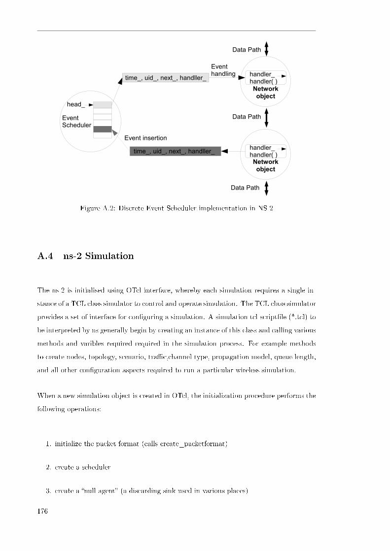
Figure A.2: Discrete Event Scheduler implementation in NS 2
A.4 ns-2 Simulation
The ns-2 is initialised using OTcl interface, whereby each simulation requires a single in-
stance of a TCL class simulator to control and operate simulation. The TCL class simulator
provides a set of interface for con�guring a simulation. A simulation tcl script�le (*.tcl) to
be interpreted by ns generally begin by creating an instance of this class and calling various
methods and varibles required required in the simulation process. For example methods
to create nodes, topology, scenario, tra�c,channel type, propagation model, queue length,
and all other con�guration aspects required to run a particular wireless simulation.
When a new simulation object is created in OTcl, the initialization procedure performs the
following operations:
1. initialize the packet format (calls create_packetformat)
2. create a scheduler
3. create a �null agent� (a discarding sink used in various places)
176
A.4.1 Packet
Packet is a subclass of the class event. Objects in the Packet class are the fundamental unit
in exchange between objects. NS-2 packet is composed of stack of headers and optional
data space, which is initialised when a simulator object is created. So a network object
can access any header in the stack of a packet it processes it using o�set value.
The initialization of the packet format will set up the �eld o�sets used for the entire
simulation. Given that ns-2 is an event-driven simulator, from this point on, the scheduler
takes over.
A null agent is created to act as a sink for packets, both successfully transmitted and
dropped. Packets may be handled to NsObjects at scheduled points in time since a node is
an event handler and task performed over a packet is an event. Tasks over a packet should
the only type of event scheduled on a node.
Testing protocols under an appropriate set of network conditions is critical in achieving
valid and meaningful results. Using automatic created complex scenarios can help to
achieve such appropriate scenarios. In ns-2, a scenario de�nes the input con�guration for
the simulator to run. A Scenario is made up of several components including network topol-
ogy and tra�c model. The network topology include the physical interconnects between
nodes and the static characteristics of links and nodes. The tra�c model de�nes the net-
work usage patterns and unicast and multicast senders locations. The key challenge in the
topology generation is coming up with a topology that embodies relevant characteristics.
For example, TCP and CBR tra�c between mobile nodes can be setup manual or by using
random tra�c connections using CMU's tra�c-scenario generator scripts available under
ns-2.34/indep-utils/cmu-scen-gen, called cbrgen.tcl and tcpgen.tcl. These scripts can be
used to generate CBR or TCP tra�c connections between wireless nodes respectively by
using the following command:
ns cbrgen.tcl [-type cbr/tcp] [-nn nodes] [-seed seed] [-mc connections]
[-rate rate]> file_to_store
177

A.4.2 Scenario and mobility models
In order to carry meaningful study and di�erent network analysis such as performance of
MAC protocol, e�ect of network dynamics, scalability etc it is important to carry simulation
on the right kind of scenario, which includes but is not limited to topology size, density
distribution, tra�c generation, membership distribution, real-time variance of membership,
and network dynamics.
Di�erent scenario generated may be used to emphasise the di�erent design criterion while
studying protocol behaviour.
Nodes positions can be set manually inside tcl script or generated from a scenario �le. The
scenario �le containing the positions of all nodes. Currently there are a number of scenario
�les in ns that can be used. These are simple text �les that can be easily edited to place
the nodes at desired positions.
For large topologies, node position, movement and tra�c are de�ned in separate �les for
convenience. These �les are generated using CMU's movement and connection generations
found in ns-2.x/indep-utils/cmu-scen-gen/setdest.
The scenario generator �le command allows one specify number of nodes in the simulation,
x and y position of the node with respect to topology dimension, and distance from the
coordinator, used main for single hop. By running
scen_gen [number of nodes] [x-position coordinate] [y- position
coordinate][personal operating space]
will produce a �le wpan.scn, to be used in source scenario �le (*.tcl)
For mobile node scenario we can run:
./setdest -n [number of nodes] -p [pause time] -M [maximum speed]
-t [simulation time] -x [max x] -y [max y]> [output dir]/[scenario-file]
for version 1.
178
A.4.3 NS 2 mobile node model
A simple unicast node consists of Two TclObjects: an address classi�er (classi�er_) and
a port classi�er (dmux_). The main function of these classi�ers is to distribute incoming
packets to the correct agent or outgoing link. By default nodes in ns are constructed for
unicast simulations. In order to enable multicast simulation, the simulation should be
created with an option �-multicast on�, i.e. set ns [new simulator -multicast on]
The function �Simulator::node-con�g{}� accommodates �exible and modular construction
of di�erent node de�nitions within the same base Node class.
To create a node capable of wireless communication we use wireless communication con-
�guration support
$ns_ node-config -adhocRouting dsdv
It is essential to de�ne the node characteristics through con�guration before creating them.
This includes the address structure, type of routing and energy model.
Mobile nodes are derived from the basic ns Node object with added functions such as
movement or mobility, periodic position updates, ability to maintain topology boundary
and ability to transmit and receive on a channel that allows it to be used to create mobile,
wireless simulation environments.
The network stack for mobile node consists of link layer (LL), an ARP module connected
to LL, an interface priority queue (IFq), a mac layer (MAC), a network interface (netIF),
all connected to the channel.
In the wireless model the core of the simulation environment generally consists of a mobile
node with additional support features allowing simulation of multi-hop ad-hoc networks,
wireless LANs and other networks. NS nodes support other added functionalities like
movement, and power management. When creating mobile nodes in NS-2 environment
�rstly one needs to create a mobile node object, secondly the mobile node must be con�g-
ured by creating a particular ad-hoc-routing agent that will be used by the node or nodes,
next the network stack consisting of a link layer, interface queue, mac layer, network inter-
face with an antenna, and propagation model must be created, we then interconnect these
components and lastly, connect the stack to the channel.
179

The class MobileNode is used too simulate wireless nodes in wireless ad hoc networks or
sensor networks on wireless channel. The class MobileNode inherits from the class Node,
however there are no links in MobileNode, the receiving and sending packets are based on
Wireless Channel not links
Figure A.3 illustrates the schematic of a mobile node under the CMU monarch wireless
extension to NS. Note the mobile structure used in the case of DSR protocol is slightly
di�erent.
Figure A.3: Schematic node extended to implement mobile node
A.5 Extending New Implementation/Coding
Using doxygen or similar software, the ns-2 class hierarchy for 802.15.4 protocol standard
or any other protocol can easily be revealed. A protocol implementation in a ns-2 follows
object oriented approach. Therefore any changes or implementation of code needs to be
done in a structured manner.
The overall documentation for 802.15.4 exist in NS-2 implementation. In this section, the
fundamental of extending the 802.15.4 standard protocol is described as follows:
180

� Derive class from mac and/or wirelessPhy
� Create C++ class, �ll the methods
� De�ne OTcl linkage if any -In order to access private variables you need to export
the C++ variables to OTcl as follows
� Write OTcl code if any
� Save the new *.h and *.cc �les in ns-2.34 directory
� Edit the Make�le of ns-2.34 directory to add the object �le newagent.o
� Execute �make� command
� Build and debug the code
� Test using tcl script
The folder containing all modi�cation is added in the ns-2.34 folder, then one needs to
make few more changes such as editing the Make�le by adding new object �les inside
OBJ_CC variable before recompiling ns-2.
A.5.1 Linking C++ implementation and OTcl objects
Modi�cation and implementation done in C++ are only accessible through Tcl script if
there are bond. To bind our implementation to Tcl interface so that our implementation
can be instantiated from Tcl. To do this we use the class TclClass, for example:
stat ic class p804_15_4new : public TclClass {
public :
p802_15_4new ( ) : Tc lClass ( 8 02 . 1 5 . 4new){}
TclObject * c r e a t e ( int argc , const char*const* argv ){
return (new 802 . 15 . 4new)
}class_p802_15_4new
//
Although most of the binding is done when a class object is initiated, the other way to
establish link between OTcl and compiled C++ objects is to use binding funstion. The
binding function takes to argunments, the name of the OTcl variable and the address of
the C++ compiled variable.
181
� De�ne the newAgent class in C++
� In C++ class de�nition:De�ne a static class, NewAgentClass that inherits the class
�TclClass� that aims to de�ne a new OTcl object of speci�ed name and make a linkage
between this OTcl object and C++ object
� In order to access private variables you need to export the C++ variables to OTcl as
follows
� Save the newagent.h and newagent.cc in ns-2.34 directory
� Edit the Make�le of ns-2.34 directory to add the object �le newagent.o
� Execute �make� command
� Run the newagent.tcl script
A.5.2 Debugging and variable tracing
In NS 2 architecture, programming error can be classed into runtime errors and C++
compilation errors. Run time errors occur during NS 2 simulation caused by error in OTcl
or/and C++ programming. Compilation errors occur during the compilation process when
C++ header and source �les are converted into object �les with the extension �.o� and
when compiler links the created object �les to create NS executable �le. In the case of the
compilation process, errors may occur if the compiler is unable to understand the C++
codes. The compiler will show error messages on the screen, indicating where and why the
error occurred. Examples of compilation errors include incorrect C++ syntax and a use
of unde�ned variable and/or function. In the case of when compiler links created objects,
error may occur due to improper linkage of C++ �les. Example of linking error include
instantiate an object from an abstract class and modifying a base class without creating
object �les of the child classes whereby this error usually occurs when dependency in the
Make�le is not properly de�ned.
A.6 Extracting Information from the Trace Files
Compilation of simulation results refers to the process of collecting information from sim-
ulation and compute performance measures under consideration. There are three main
182

approaches to collect simulation results in NS2, include through C++ code, through Tcl
codes and through trace �le.
The trace �le format de�nes how the variable details are recorded in a trace �le. The
format of the �le is de�ned in a function trace(v) of the class TclObject.
Upon simulating a particular scenario, trace �les recording detailed information on events
such as tra�c and information about mobile nodes are generated. Awk scripts were then
used in order to analyse or extract relevant information or measure a particular metric from
the trace �les. Figure A.4 shows the format of an example trace �le (new trace format). In
the trace �le each column separated by a space represents some information, for example
here we have a packet sent(s) at time (-t) sec, from source node (Hs) 0 to destination node
(Hd) 1. The source node id (Ni) is 0, the node x, y and z coordinates are speci�ed by
(Nx), (Ny) and (Nz) respectively. The node energy level (Ne) is 19.986414$J$, the trace
level (Nl) is RTR (shows the network level). The node event (Nw) is blank. The MAC
level information is given by duration (MA) 0, destination Ethernet address (Md) 0, the
source Ethernet address (Ms) is 0 and Ethernet type (Mt) is 0. Following the MAC level
information is the IP packet level information like packet id (li), source (address.source
port number) given by (Is) and the destination (address.destination port number) is given
by (Id).
Figure A.4: Trace �le output format (new trace format)
A.7 Simulation Visualization
NS comes with animation tool called Network Animator. We used Network animator
(NAM) to visualize mobile node position, direction of movement and speed. NAM is
animation tool that comes with NS 2 for viewing network simulation traces and real world
packet trace data. NAM is designed to read simple animation event commands from a
large trace �le. Xgraph, Excel or Gnuplot can be used to plot graphs. Figure A.5 shows a
typical NAM display with a coordinator in the middle of surrounding nodes.
183

Figure A.5: NAM
184