HAL Id: hal-01237935https://hal.archives-ouvertes.fr/hal-01237935

Submitted on 8 Dec 2015

HAL is a multi-disciplinary open accessarchive for the deposit and dissemination of sci-entific research documents, whether they are pub-lished or not. The documents may come fromteaching and research institutions in France orabroad, or from public or private research centers.

L’archive ouverte pluridisciplinaire HAL, estdestinée au dépôt et à la diffusion de documentsscientifiques de niveau recherche, publiés ou non,émanant des établissements d’enseignement et derecherche français ou étrangers, des laboratoirespublics ou privés.

On a Model of Pattern Regeneration Based on CellMemory

Nikolai Bessonov, Michael Levin, Nadya Morozova, Natalia Reinberg, AlenTosenberger, Vitaly Volpert

To cite this version:Nikolai Bessonov, Michael Levin, Nadya Morozova, Natalia Reinberg, Alen Tosenberger, et al.. On aModel of Pattern Regeneration Based on Cell Memory. PLoS ONE, Public Library of Science, 2015,�10.1371/journal.pone.0118091�. �hal-01237935�

On a Model of Pattern RegenerationBased on Cell Memory

N. Bessonov1, M. Levin2, N. Morozova3, N. Reinberg1,A. Tosenberger4, V. Volpert4

1 Institute of Problems of Mechanical Engineering, Russian Academy of Sciences199178 Saint Petersburg, Russia

2 Department of Biology, Tufts Center for Regenerative & Developmental BiologyTufts University, Medford, MA 02155, USA

3 Laboratoire Epigenetique et Cancer, CNRS FRE 3377, CEA Saclay, France4 Institut Camille Jordan, UMR 5208 CNRS, University Lyon 1, 69622 Villeurbanne, France

Abstract. The paper is devoted to modelling of regeneration of biological organisms. Bi-ological cell structures are considered as ensemble of mathematical points on the plane.Each cell produces a signal which propagates in space. It is received by other cells. Totalsignal received by each cell forms a signal distribution defined on the cell structure. Thisdistribution characterizes the geometry of the cell structure. If a part of this structure isremoved, then remaining cells have two signals. They keep the value of the signal whichthey had before the amputation (memory), and they receive a new signal produced afterthe amputation. Regeneration of the cell structure is stimulated by the difference betweenthe old and the new signals. It is stopped when the two signals coincide. The algorithmof regeneration contains certain rules which are essential for its functioning, being the firstquantitative model of cellular memory that implements regeneration of complex patterns toa specific target morphology. Correct regeneration depends on the form and on the size ofthe cell structure and on parameters of regeneration.

Key words: regeneration, cell memory, signal distribution

1 Introduction

Numerous species are able to restore complex body organs after amputation (Birnbaum andAlvarado, 2008). For example, planaria can regenerate their entire body from a small frag-ment (Reddien and Snchez Alvarado, 2004), and axolotls can restore limbs, spinal cord, jawseyes, hearts, and portions of their brain (Maden, 2008). Learning to control this process isthe key to transformative applications in biomedicine (Baddour et al., 2012; Levin, 2011).While the field is rapidly accumulating high-resolution data on the genetic networks neces-

1

sary for this process (Stocum and Cameron, 2011), fundamental insight into complex shapehomeostasis is lacking. This is related to a dearth of testable models explaining the signal-ing dynamics sufficient to explain how the correct pattern is regenerated and how growthceases when the proper anatomy is restored. One of the main open questions is whether theregenerating organism uses only the information available at each particular moment of timeor whether it can also use information about its former state – a pattern memory (Kraglet al., 2009; Kragl et al., 2008). In the first case, in order to reproduce complex forms anddifferent organs, we need to deal with pattern formation and emergence of forms. This isoften modeled via Turing structures and other mechanisms of pattern formation and self-organisation (Badugu et al., 2012; Belintsev et al., 1987; Economou et al., 2012; Kusch andMarkus, 1996; Meinhardt, 2010; Rauch and Millonas, 2004; Schiffmann, 2007). The processof regeneration becomes regeneration of patterns. If this pattern corresponds to a stationarysolution of a reaction-diffusion model, then amputation can be considered as a perturbationof this stationary solution and regeneration corresponds to decay and disappearance of thisperturbation.

In contrast, the organism may keep information about its original state and restorespattern after damage by minimizing the difference between the current state and the originalstate (a target morphology model) (Levin, 2011, 2012; Vandenberg et al., 2012). At this time,no quantitative model of target morphology during pattern formation exists.

In this work we suggest a mathematical model based on the assumption that regenerationuses the memory of the organism about its original state. This model provides a proof-of-principle of a mechanistic model that implements patterning towards an encoded targetmorphology memory, and illustrates a system to formulate the assumptions necessary forregeneration of cellular structures in mathematical models.

The scheme presented below is based on the assumption that there are cells that canpreserve information during some time (memory cells). This is realistic since a wide varietyof somatic cell types, not only neurons, have been shown to exhibit memory (Casadesus,2002; Chang, 2002; Nakagaki, 2001; Hamilton, 1975; Applewhite, 1975; Eisenstein, 1975).We model it as follows. Suppose that a cell receives some signal u with a given intensityu = u∗ (this could be concentration of a signaling molecule, or a bioelectric signal (Levin,2014; Levin and Stevenson, 2012), or any other kind). After some time, when the signaldisappears or changes its value, the information about the old value u∗ is preserved in thecell. Moreover, we presume that the cell can measure the difference between the old valueand the current (new) value, u∗ − u, and produce another signal z with a rate proportionalto this difference.

There are various kinds of cells that exhibit memory (neural cells, lymphocytes, plants,bacteria) via different mechanisms. These assumptions do not contradict available biolog-ical information but it is not yet known whether memory processes operate during tissueregeneration. Our model provides testable predictions for this idea.

We suggest a possible mechanism which can provide these properties. Let the signal ucorrespond to the concentration of some substance A in a volume bounded by a membrane.Its value in this volume equals u∗ and is kept fixed. At the other side of the membrane

2

u = 0. Its flux through the membrane is proportional to the difference of the values, thatis to u∗ . This flux leads to the appearance of stable objects B (ion channels, molecules)which participate in processing of A (transport, consumption, reaction). The quantity of Bis proportional to the flux of A, that is to u∗. If u decreases, then some part of B is liberatedfrom processing of A and becomes involved in other reactions. They lead to production ofanother signal z. This mechanism keeps memory either about the maximal value = u∗ orabout the value which is kept during some time sufficient to create B.

We note that the mechanisms which allow cells to determine and to preserve the maximalsignal was suggested and discussed by H. Meinhardt (Meinhardt, 2010).

The signals can be transported either from cell to cell proportionally to the difference ofconcentrations or by diffusion through the extracellular matrix.

The implementation of the model is based on the method of cellular automata wherecells are located at the nodes of a square grid. Cells communicate with each other due tothe exchange of signals and they can divide according to some algorithm described in thenext section. Cellular automata are widely used to model growth of biological tissues (seeDeutsch and Dormann, 2005, and the references therein). Tissue regeneration is studiedin a more general Neuronal Organism Evolution model (Astor and Adami, 2000; Hamptonand Adami, 2004). The main objective of this work is to develop a minimal model of tissueregeneration based on plausible biological assumptions and allowing the exact regenerationof an arbitrary (in some limits) amputated part of the tissue.

2 Model of regeneration

2.1 Signal distribution

Consider a 2D domain D filled by cells. Each cell produces a signal u which spreads in space.Its intensity decays with distance as some function f(d). If the distance between cell i (Ci)and cell j (Cj) is dij, then Cj receives signal f(dij) from Ci. We will assume here that eachcell produces the same signal. Therefore Ci receives from Cj a signal of the same intensityf(dij). For each cell Ci we can count the total signal which it receives from other cells

ui =∑j =i

f(dij). (2.1)

We will use also the notation u(x) assuming that x belong to the domain D, ui = u(xi),where xi is the coordinate of the ith cell.

Clearly, cells located in different part of the domain will receive different signals. Forexample, a cell located at the boundary receives signals only from one side and the valueof the signal can be less than for a cell inside the domain. Therefore the distribution u(x)represents some information about the geometry of the domain.

Let us consider some examples. Signal distribution for a rectangular domain is shownin Figure 1. Here f(d) = 1/d2. The value u(x) at the boundary is less than inside the

3

Figure 1: Rectangular domain filled by cells (left). The value of the signal in each cell (right),f(d) = 1/d2.

domain, and the value at the corners is less than in other points of the boundary. The signaldistribution depends on the function f(d) (Figure 2).

Figure 2: Signal distribution for f(d) = 1/d0.5.

2.2 Reduction of the domain

Suppose that a part of cells is removed (white cells in Figure 3). The remaining cells will becalled control cells. We can define two signals in control cells: the old signal

u∗i =

∑j =i,j∈I0

f(dij), i ∈ Ic,

4

where I0 is the set of cells in the original cell structure, Ic is the set of control cells, and thenew signal

ui =∑

j =i,j∈Ic

f(dij), i ∈ Ic.

The old signal is measured in control cells from all cells in the original structure before am-putation. The new signal is measured also in control cells which they receive from remaining(control) cells after amputation. These two signal distributions are different. The differenceis clearly seen near the cut (Figure 4).

Figure 3: A part of cells is removed. White cells show places of removed cells. Red cells arethe remaining cells which are at the boundary with the removed cells (blastema).

Figure 4: Signal distribution in control cells for the complete structure (left) and for thereduced structure (right).

2.3 Updating cells: analytical examples

When a part of cells is removed, the signal distribution in the remaining cells, which we callcontrol cells, is changed. Then the question is how to restore the cell configuration with the

5

initial signal distribution. Remaining cells near the cut will start to divide. New cells willcontribute to the signal distribution and will continue to divide filling available places intheir neighborhood. This growing structure is regulated by the signal distribution in controlcells and will converge to the initial structure.

We will begin with some simple examples that admit analytical solutions. Consider threecells, A, B and C. Let us remove the cell C and discuss the algorithm of its restoration.Denote by dAB, dBC and dAC the distances between the corresponding cells. Before removalthe cell C, the signals received by cells A and B are as follows:

u∗A = f(dAB) + f(dAC), u∗

B = f(dAB) + f(dBC).

When this cell is removed, they become

uA = f(dAB), uB = f(dAB).

We put cell C in an arbitrary place and denote by dBC and dAC its distances to the cells Aand B. The new signals received by these cells are now

uA = f(dAB) + f(dAC), uB = f(dAB) + f(dBC).

We need to choose the position of cell C in such a way that uA = u∗A, uB = u∗

B. Theseequalities are satisfied if

f(dAC) = f(dAC), f(dBC) = f(dBC).

Since f(d) is a monotonically decreasing function, we conclude that dAC = dAC , dBC = dBC .These equalities determine two circles on the plane. One of them is around point A withradius dAC , another one is around point B with radius dBC . They intersect in two points.One of them corresponds to the initial position of cell C, and another one is symmetric withrespect to the line AB.

Thus, in the case of three cells, one removed cell can be restored by a simple algorithmdescribed above. A similar approach is applicable for any initial number of cells n if onlyone cell is removed. It should be noted that in general n − 1 circles may not have a pointof intersection. However in the problem considered here their intersection is guaranteed bythe initial configuration.

If more than one cells are removed, the problem of their restoration does not have a simpleanalytical solution except for the case where all cells are located at the same straight line.The existence of solutions of the restoration problem is provided by the initial configuration.So the question is how to converge to this configuration adding new cells one after another.A possible algorithm is suggested in the next section.

2.4 Algorithm of regeneration

We will use the difference between the signals u∗i and ui, i ∈ Ic in order to restore the initial

form. The question here is about the algorithm of choice that determines where to put new

6

cells. We will add new cells one after another and denote the set of cells in the process ofregeneration by I(t). Here t is discrete time, t = tn, where at each next time step we addone cell. Let us introduce the signal

ui(t) =∑

j =i,j∈I(t)

f(dij), i ∈ Ic.

This means that we measure the total signal from old and new cells in the control cells. Thepurpose is to restore a structure for which

ui(T ) = u∗i , i ∈ Ic

for some time t = T .

We suggest an algorithm for the placement of new cells. It is determined by the followingthree conditions:

1. All cells are placed in the nodes of the square grid. Each cell has 8 neighbors, 4 of themwith a common side and 4 other cell with a common diagonal. Each new cell is placed insuch a way that among its neighbors there is at least one cells from the cut (blastema) oranother new cell. This condition provides continuity of growth of the regenerating domain,beginning from the place of the cut,

2. When we add a new cell we recalculate the signal in every control cell. The new signalshould be less than or equal to the old signal,

ui(t) ≤ u∗i , i ∈ Ic.

In numerical simulations this condition should be satisfied with certain accuracy (Section3.1).

3a. Let us introduce total signals:

S∗ =∑i∈Ic

u∗i , S(t) =

∑i∈Ic

ui(t).

Among all cells, which satisfy conditions 1 and 2, at each time step we choose the cell forwhich the difference S∗ − S(t) is minimal.

Let us illustrate this condition with the following example. Suppose that there are onlytwo control cells A and B, and we choose where to place a new cell C. For each possibleposition of cell C, we measure the signal S(AC) received by cell A from cell C and the signalS(BC) received by cell B from cell C. We put cell C in the place where the sum of thesetwo signals is maximal.

3b. Each control cell produces a signal proportional to the difference u∗i − ui(t). This signal

spreads in space and stimulates appearance of new cells. We choose the cell, which satisfiesconditions 1 and 2, and where the value

7

zk =∑i∈Ic

f(dik)(u∗i − ui(t))

is maximal. Here k belong to the set of cells, which satisfy conditions 1 and 2.

Conditions 3a and 3b give close results. In the first case, we choose the cell which addsthe greatest signal to the control cells. In the second case, we choose the cell which getsthe greatest signal from the control cells. The second algorithm is more justified from thebiological point of view.

Figure 5: The choice of the first cell. Black dots show possible candidates for new cells. Twocases are presented: with condition 2 (left), without condition 2 (right). Arrows show twoadditional candidates which appear without condition 2.

Let us illustrate how the algorithm of cell choice works in the example shown in Figure 5.According to condition 1, we consider all cells at the nodes of the grid near the cut (red cells).They are marked with black dots in the figure. Next, we verify that they satisfy condition2. Some of them may not satisfy it. Figure 5 (right) contains two additional candidates incomparison with Figure 5 (left). This small difference appears to be crucial. We will seethat condition 2 is necessary for normal regeneration. Finally, among all candidates, whichsatisfy conditions 1 and 2, we choose the first new cell according to condition 3a or 3b.

Continuation of the regeneration without condition 2 is shown in Figure 6. When thefirst row is filled, the best cell according to condition 3a is in the middle of the secondrow. However, condition 3b favors a cell at the continuation of the cut row (the last rowof remaining cells). The algorithm with condition 3a (without condition 2) shows a betterregeneration. New cells fill 5 rows of the original form and then it adds a cell outside theoriginal form. Yellow cells show the places where condition 2 is not satisfied. The blue isthe worst among such cells, that is where the difference ui − u∗

i is maximal.If we use condition 2, then both algorithms (3a and 3b) correctly regenerate the original

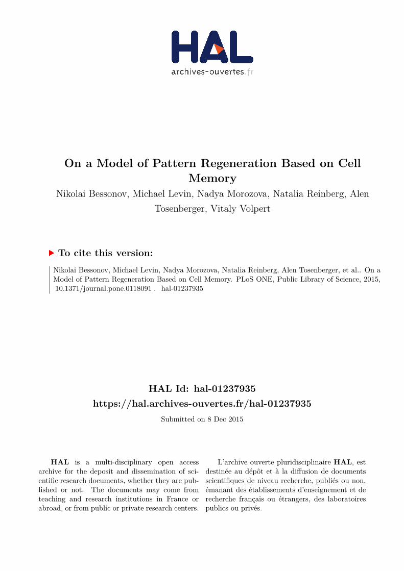
form (Figure 7). Figures 8 and 9 show the evolution of the new signal ui(t) in the control

8

Figure 6: Regeneration without condition 2 and with condition 3a (left) or 3b (right).

Figure 7: Regeneration with condition 2 and two different amputated parts. Both algorithms3a and 3b give the same result.

cells during regeneration. It gradually grows and after the regeneration of several dozens ofcells it comes close to the old signal.

Figure 8: New signal in control cells before regeneration (left) after regeneration of 5 cells(right).

9

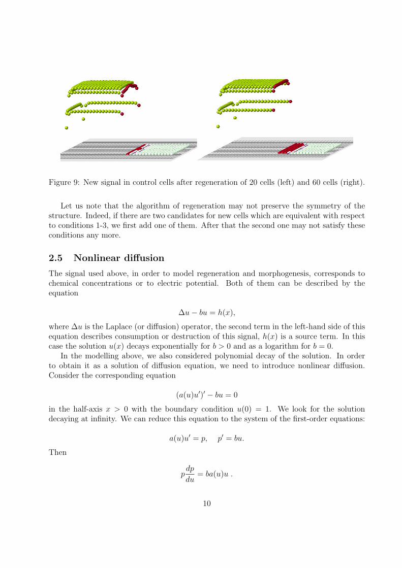
Figure 9: New signal in control cells after regeneration of 20 cells (left) and 60 cells (right).

Let us note that the algorithm of regeneration may not preserve the symmetry of thestructure. Indeed, if there are two candidates for new cells which are equivalent with respectto conditions 1-3, we first add one of them. After that the second one may not satisfy theseconditions any more.

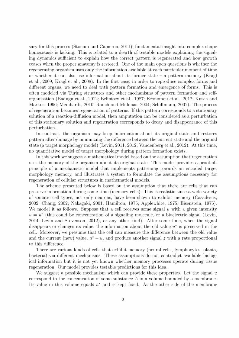
2.5 Nonlinear diffusion

The signal used above, in order to model regeneration and morphogenesis, corresponds tochemical concentrations or to electric potential. Both of them can be described by theequation

∆u− bu = h(x),

where ∆u is the Laplace (or diffusion) operator, the second term in the left-hand side of thisequation describes consumption or destruction of this signal, h(x) is a source term. In thiscase the solution u(x) decays exponentially for b > 0 and as a logarithm for b = 0.

In the modelling above, we also considered polynomial decay of the solution. In orderto obtain it as a solution of diffusion equation, we need to introduce nonlinear diffusion.Consider the corresponding equation

(a(u)u′)′ − bu = 0

in the half-axis x > 0 with the boundary condition u(0) = 1. We look for the solutiondecaying at infinity. We can reduce this equation to the system of the first-order equations:

a(u)u′ = p, p′ = bu.

Then

pdp

du= ba(u)u .

10

Taking into account the boundary condition p(0) = 0, we can integrate the last equation:

p2(u) = 2b

∫ u

0

a(v)vdv.

Set a(u) = u−k. Then we get

u′ = ukp(u) = −√

2b

2− ku1+k/2 .

From this equation and the boundary condition we obtain

u(x) =1

(1 + cx)2/k, c =

k

2

√2b

2− k.

Hence solution exists for any k, 0 < k < 2. It can decay with the rate 1/xn with any n > 1.It corresponds to the decay rate considered in numerical simulations.

3 Results

3.1 Dependence on parameters

The model contains only one physical parameter, the rate of decay of the signal, and onenumerical parameter related to verification of condition 2. We consider the function f(d),which shows how the signal depends on distance, in two different forms:

f1(d) = d−n , f2(d) = e−nd ,

where n > 0. All results shown in the previous section are obtained with the first functionfor n = 2.

Figure 10: Regeneration with the algorithm 3b and f(d) = 1/dn, n = 1.6 (left), n = 2.4(right). Red cells show the regenerated domain, white cells its difference with the originaldomain, blue and yellow cells show where condition 2 is not satisfied.

11

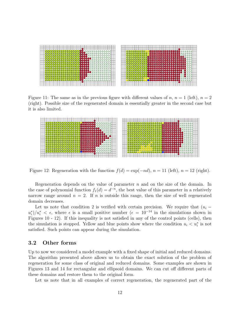
Figure 11: The same as in the previous figure with different values of n, n = 1 (left), n = 2(right). Possible size of the regenerated domain is essentially greater in the second case butit is also limited.

Figure 12: Regeneration with the function f(d) = exp(−nd), n = 11 (left), n = 12 (right).

Regeneration depends on the value of parameter n and on the size of the domain. Inthe case of polynomial function f1(d) = d−n, the best value of this parameter in a relativelynarrow range around n = 2. If n is outside this range, then the size of well regenerateddomain decreases.

Let us note that condition 2 is verified with certain precision. We require that (ui −u∗i )/u

∗i < ϵ, where ϵ is a small positive number (ϵ = 10−14 in the simulations shown in

Figures 10 - 12). If this inequality is not satisfied in any of the control points (cells), thenthe simulation is stopped. Yellow and blue points show where the condition ui < u∗

i is notsatisfied. Such points can appear during the simulation.

3.2 Other forms

Up to now we considered a model example with a fixed shape of initial and reduced domains.The algorithm presented above allows us to obtain the exact solution of the problem ofregeneration for some class of original and reduced domains. Some examples are shown inFigures 13 and 14 for rectangular and ellipsoid domains. We can cut off different parts ofthese domains and restore them to the original form.

Let us note that in all examples of correct regeneration, the regenerated part of the

12

Figure 13: For the same original cell structure we can cut off different parts and regeneratethe same original form. Red cells show the regenerated parts.

Figure 14: Regeneration of ellipse.

domain is convex or it is composed of several separated convex subdomains for which re-generation occurs almost independently. The algorithm described above is not aimed fornonconvex domains because the distance between two cells is measured along the straightinterval connecting them. If the domain is not convex and the signal propagates along thetissue, then the distance between two points should also be measured along the tissue.

13

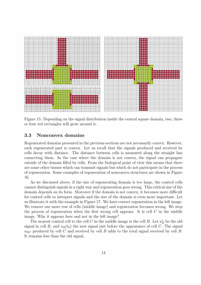
Figure 15: Depending on the signal distribution inside the central square domain, two, threeor four red rectangles will grow around it.

3.3 Nonconvex domains

Regenerated domains presented in the previous sections are not necessarily convex. However,each regenerated part is convex. Let us recall that the signals produced and received bycells decay with distance. The distance between cells is measured along the straight lineconnecting them. In the case where the domain is not convex, the signal can propagateoutside of the domain filled by cells. From the biological point of view this means that thereare some other tissues which can transmit signals but which do not participate in the processof regeneration. Some examples of regeneration of nonconvex structures are shown in Figure16.

As we discussed above, if the size of regenerating domain is too large, the control cellscannot distinguish signals in a right way and regeneration goes wrong. This critical size of thedomain depends on its form. Moreover if the domain is not convex, it becomes more difficultfor control cells to interpret signals and the size of the domain is even more important. Letus illustrate it with the example in Figure 17. We have correct regeneration in the left image.We remove one more row of cells (middle image) and regeneration becomes wrong. We stopthe process of regeneration when the first wrong cell appears. It is cell C in the middleimage. Why it appears here and not in the left image?

The nearest control cell to the cell C in the middle image is the cell B. Let u∗B be the old

signal in cell B, and uB(t0) the new signal just before the appearance of cell C. The signaluBC produced by cell C and received by cell B adds to the total signal received by cell B.It remains less than the old signal,

14

Figure 16: Regeneration of letters. Regenerated part is shown in red, remaining part afteramputation in green. The red cells adjacent to green cells belong to the remaining part(blastema).

uB(t0) + uBC ≤ u∗B. (3.2)

Therefore the second condition of the algorithm remains satisfied and cell C is added to theregenerated structure. After that regeneration continues in a wrong way (Figure 18).

15

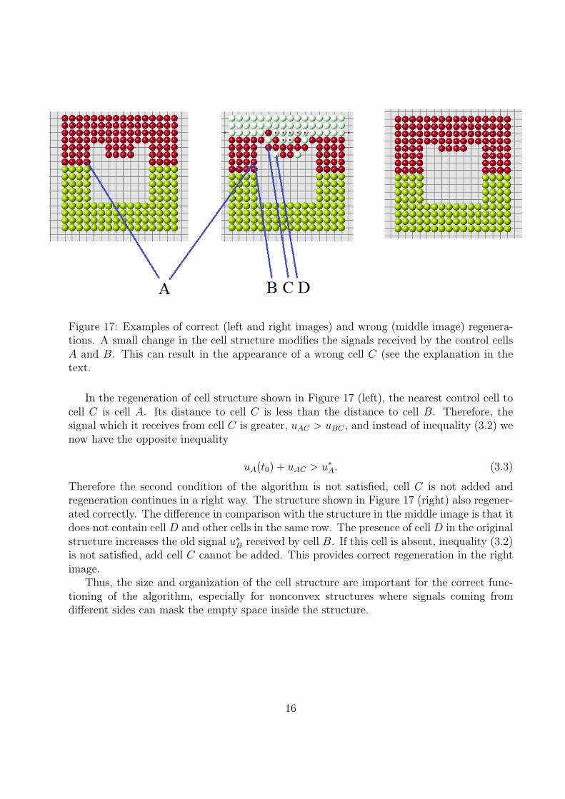
Figure 17: Examples of correct (left and right images) and wrong (middle image) regenera-tions. A small change in the cell structure modifies the signals received by the control cellsA and B. This can result in the appearance of a wrong cell C (see the explanation in thetext.

In the regeneration of cell structure shown in Figure 17 (left), the nearest control cell tocell C is cell A. Its distance to cell C is less than the distance to cell B. Therefore, thesignal which it receives from cell C is greater, uAC > uBC , and instead of inequality (3.2) wenow have the opposite inequality

uA(t0) + uAC > u∗A. (3.3)

Therefore the second condition of the algorithm is not satisfied, cell C is not added andregeneration continues in a right way. The structure shown in Figure 17 (right) also regener-ated correctly. The difference in comparison with the structure in the middle image is that itdoes not contain cell D and other cells in the same row. The presence of cell D in the originalstructure increases the old signal u∗

B received by cell B. If this cell is absent, inequality (3.2)is not satisfied, add cell C cannot be added. This provides correct regeneration in the rightimage.

Thus, the size and organization of the cell structure are important for the correct func-tioning of the algorithm, especially for nonconvex structures where signals coming fromdifferent sides can mask the empty space inside the structure.

16

Figure 18: Continuation of the wrong regeneration started in Figure 17 (middle).

4 Discussion

We suggest a model of regeneration of cell structures based on cell memory – implementedas follows. Each cell receives signals from all other cells. Its total value is u∗. The cell keepsthe memory about this value. If the total signal changes and becomes u, the cell producessome substance with the rate proportional to u∗ − u. This substance stimulates appearanceof new cells. As a result, cell structure grows until the new signal u becomes equal to theold signal u∗. This mechanism allows cells to implement a kind of means-ends analysis - aworking towards regeneration of a specific shape and a cessation of further growth when thecorrect morphology is achieved.

The main question is whether this method allows a correct regeneration of cell structurewhen a part of it is amputated. We show that under some additional conditions whichprovide continuity of growth and that the new signal cannot exceed the old signal, we canobtain an exact solution of the regeneration problem.

Limitations of the algorithm. The algorithm of cell structure regeneration suggestedin this work has several limitations. First is the size of the structure. Control cells cannotcorrectly identify missing cells at a large distance because the signal rapidly decays. If therate of decay is low, then the boundary of the cell structure is not clearly identified. Addedcell will go beyond the original structure and regeneration will be wrong. On the otherhand, rapid decay of the signal also requires high accuracy in the verification of the secondcondition of the algorithm. If the new signal in some of control cells becomes greater thanthe old one on a very small value (usually, 10−7 − 10−15), then the algorithm is stopped.Biologically this means that control cells are very sensitive. It should be noted however thatwe consider a qualitative mechanism of regeneration with arbitrary values of parameters. Sowe cannot relate them at the moment to realistic biological values.

Figures 19 and 20 show regeneration of a long thin domain for different values of param-eters and sizes of the domain. There are some optimal values where the algorithm is moreefficient. If we consider the size of the cell structure close to its maximal admissible value,

17

the algorithm becomes sensitive to small changes of parameters or geometry. In particular,if the remaining part of the domain after amputation is less than some critical value (Figure19, left), then regeneration fails.

Figure 19: Regeneration with condition 3a and different sizes of the remaining domain (left)or different decay rate n of the signal (right). The signal decays as 1/xn, n = 1.5, ϵ = 10−15.

Figure 20: Regeneration with condition 3a and different values of ϵ (n = 1.5).

Finally, let us recall that the distance between two cells is measured along the straightline connecting them. If the cell structure is not convex, then this interval can be partiallyoutside of this structure. From the biological point of view, this implies existence of othercells (not explicitly included in the model) which fill the empty space and which can transmitthe signal but do not participate in the process of regeneration. It is possible to modify the

18

algorithm is such a way that the signal propagates along the structure even in the case whereit is not convex. However it becomes essentially more complex and the path between twopoints to measure the distance between them can be defined in different ways. This will beexplored in subsequent work.

Reaction-diffusion patterns or cell memory? Reaction-diffusion systems of equationscan describe emergence of patterns. The mechanism of pattern formation mostly used inmorphogenesis and regeneration is based on Turing structures. In order to describe emer-gence of patterns, the reaction-diffusion system should contain at least two equations andshould satisfy some additional conditions. They are formulated by H. Meinhardt as shortrange activation - long range inhibition. Emergence of patterns is based on the interaction ofthese two substances (Turing called them morphogens). Since these patterns can representstable stationary solutions, then the perturbed pattern can return to its original form aftersome time. This is the main idea of regeneration models with reaction-diffusion equations.

Some animals, like planarian or hydra, can regenerate their head or tail (feet) or both.These two organs can produce various signals which propagate in other tissues. If thesesignals interact with each other (activation-inhibition) and if this interaction results in theirnonuniform distribution (pattern formation), then it is possible to imagine that they alsoparticipate in the regeneration of the lost organ.

The method suggested in this work does not imply the interaction of two (or more)signals. In the minimal configuration it is sufficient to have only one signal. The mainassumption of the model is that cells can keep information about the previous value of thissignal when it is changed (< 64 bits of information). One testable prediction of such modelsis that mechanisms that underlie memory in the nervous system may be likewise implicatedin regenerative pattern control.

Let us note that regeneration with memory cells acts locally. It does not require inter-action of signals from distant organs. Wound healing is an example of regeneration whichoccurs locally and where only one tissue can be involved. The model based on cell memorysuggests the same approach to wound healing and to regeneration of a single organ or severalorgans simultaneously.

Let us recall that planarian possesses high morphological plasticity. It is possible inparticular to create a two-headed animal from a normal one by perturbing the physiologicalcircuit that normally determines anterior-posterior polarity (Oviedo, 2010; Beane at el.,2011). This stability of a radically new target morphology (2 heads) does not require genomicmodifications. The old one-headed and the new two-headed animals have the same genome.Moreover the new head can be grown anywhere on the body. If one of the two heads orboth of them are removed, they regenerate in the same way as they were before. Thus,two-headed planarian regenerates in a two-headed planarian with the same head locations.

It is interesting to compare how different models can regenerate a two-headed planarian.Denote by D1 the cell structure which corresponds to one-headed planarian and by D2 thetwo-headed one. After head amputation in the former, the corresponding domain is denotedby D. It is possible to amputate both heads of the two-headed animal reducing domain D2

19

to the same domain D. Hence we have the same cell structure D from which we should beable to regenerate either one-headed or two-headed planarian.

Suppose that regeneration is based on emergence of patterns. Then there are two signalsu and v which remain in the domain D after head amputation. Their interaction can producesome nonhomogeneous distribution of these substances by the mechanism of Turing struc-tures. Since the characteristic diffusion time is much less (hours) than time of regeneration(days), we can reasonably assume that they will converge to some stationary distributionsin the domain D before it begins to grow due to regeneration. If this stationary distributionis unique, then only a unique structure can regenerate and not two different structures withone and two heads. However, it is known that Turing structures in the same domain andfor the same values of parameters can be nonunique. If there are two different structurespossible in the domain D, then one of them can correspond to the one-headed animal whileanother one to the two-headed planarian. Convergence to these stationary solutions dependson the initial conditions. Since the distributions of u and v in D after amputation from D1

can differ from those after amputation from D2, then we can suppose that they will convergeto two different stationary solutions. Thus, up to now, this approach admits regeneration oftwo different structures D1 and D2 from the same reduced structure D.

The point where this approach becomes limited is that position of the second head can bearbitrary in some range of locations. If each head position should correspond to a differentstationary solution in the same domainD, then we need to have possibly many such solutionsor even a continuous family of such solutions. It is possible to have several different Turingstructures in the same domain but if there are several dozens, then it becomes exotic from themodelling point of view and unrealistic biologically. A continuous family of such solutions isnot possible even mathematically unless the domain possesses some special symmetry.

These arguments should not be considered as a proof of impossibility of this mechanismof planarian regeneration. Such complex and poorly understood processes always leave apossibility for different modelling approaches. On the other hand, the method with cellmemory eagerly reproduces two-headed or multi-headed structures with any head location(Figure 21).

Morphogenesis. The model of regeneration discussed above is based on the assumptionthat cells can register a signal coming from other cells. When a part of the tissue is am-putated, the signal is changed. The process of regeneration consists in restoring the tissuewhich has the same distribution of signals.

A similar approach can be used to describe initial tissue growth. Consider a domainfilled by cells. Suppose that each cell has some value u∗

i prescribed to it. This hypotheticalsignal appears in the process of embryogenesis due to some genetic and epigenetic factors. Itcan correspond to distribution of some morphogenes. This initial domain can be consideredas an organizing center. The signal distributed inside it stimulates appearance of new cellsaround it. These new cells will be placed in such a way, that the signal which they producecoincide with u∗

i inside the organizing center.An illustration of this mechanism is shown in Figure 15. The initial domain is a square

20

Figure 21: The same reduced part (upper left) can regenerate different original forms (upperright and lower figure).

at the center. Depending on the distribution of the signal inside this domain, differentstructures can grow from it.

Morphogenesis versus regeneration. The speed of animal regeneration can be greaterthan the speed of its natural growth. If a 7-day old tadpoles tail is cut and allowed toregenerate for 7 more days, then new tail produced will be appropriate in size for a 14-day sized animal. It shows that remaining cells remember the size of the animal beforeamputation. Moreover, this is also an argument against the pattern formation mechanism.If growth is completely determined by the actual cell structure, then natural growth andgrowth after amputation would be the same if they start from the same cell configuration.

Target morphology. The concept of target morphology is suggested in (Levin, 2011, 2012;Vandenberg et al., 2012). The model developed in this work interprets this idea in terms ofsignals. Let us recall the main assumption of the model. Control cells keep the informationabout the old signals. At the same time they receive new signals from the growing tissue.Target morphology is the morphology for which the distribution of new signals coincides withthe distribution of old signals. In the case of morphogenesis, instead of old signals, thereis some given distribution which appears during embryo development. As before, targetmorphology is the morphology for which the distribution of received signals coincides withthe given distribution. Our conjecture is that generically the target morphology is unique,that is there exists a unique solution of the problem of minimization of signal difference.

21

Further developments. If regeneration is based on cell memory in the remaining tissue,then the process of regeneration can be modified if this memory is modified. Future workin our group will test this model using reagents known to modify cellular memories in thenervous system, applied to regeneration assays.

There are many possible developments of the model. Among them introduction of differ-ent cell types (differentiation) and the model of long distance regeneration. Both of them willrequire introduction of several signals. At further stages of the development of this modelit can be possible to consider biological cells as distributed objects (not as mathematicalpoints) and associate signals to the points at the surface of their exterior membrane.

References

Astor, J.C., Adami, C. 2000. A Developmental model for the evolution of artificial neuralnetworks. Artificial Life 6, 189218.

Baddour, J.A., Sousounis, K., Tsonis, P.A., 2012. Organ repair and regeneration: anoverview. Birth Defects Res C Embryo Today 96, 1-29.

Badugu, A., Kraemer, C., Germann, P., Menshykau, D., Iber, D., 2012. Digit patterningduring limb development as a result of the BMP-receptor interaction. Sci Rep 2, 991.

Beane, W. S., Morokuma, J., Adams, D. S., and Levin, M., (2011), A chemical geneticsapproach reveals H,K-ATPase-mediated membrane voltage is required for planarian headregeneration. Cell Chemistry and Biology, 18: 77-89.

Belintsev, B.N., Beloussov, L.V., Zaraisky, A.G., 1987. Model of pattern formation in ep-ithelial morphogenesis. J Theor Biol 129, 369-394.

Birnbaum, K.D., Alvarado, A.S., 2008. Slicing across kingdoms: regeneration in plants andanimals. Cell 132, 697-710.

Casadesus, J., DAri, R, 2002. Memory in bacteria and phage. BioEssays 24:512518.

Deutsch, A., Dormann, S., 2005. Cellular automaton modeling of biological pattern forma-tion : characterization, applications, and analysis. Birkhauser, Boston.

Economou, A.D., Ohazama, A., Porntaveetus, T., Sharpe, P.T., Kondo, S., Basson, M.A.,Gritli-Linde, A., Cobourne, M.T., Green, J.B., 2012. Periodic stripe formation by a Turingmechanism operating at growth zones in the mammalian palate. Nat Genet 44, 348-351.

Hampton, A.N., Adami, C., 2004. Evolution of robust developmental neural networks. Proc.Artif. Life 9, 438-443.

Kragl, M., Knapp, D., Nacu, E., Khattak, S., Maden, M., Epperlein, H.H., Tanaka, E.M.,2009. Cells keep a memory of their tissue origin during axolotl limb regeneration. Nature460, 60-65.

Kragl, M., Knapp, D., Nacu, E., Khattak, S., Schnapp, E., Epperlein, H.H., Tanaka, E.M.,2008. Novel insights into the flexibility of cell and positional identity during urodele limbregeneration. Cold Spring Harb Symp Quant Biol 73, 583-592.

22

Kusch, I., Markus, M., 1996. Mollusc shell pigmentation: Cellular automaton simulationsand evidence for undecidability. J Theor Biol 178, 333-340.

Levin, M., 2011. The wisdom of the body: future techniques and approaches to morpho-genetic fields in regenerative medicine, developmental biology and cancer. Regenerativemedicine 6, 667-673.

Levin, M., 2012. Morphogenetic fields in embryogenesis, regeneration, and cancer: non-localcontrol of complex patterning. Bio Systems 109, 243-261.

Levin, M., (2014), Endogenous bioelectrical networks store non-genetic patterning informa-tion during development and regeneration, Journal of Physiology, 592(11): 22952305.

Levin, M., and Stevenson, C., (2012), Regulation of Cell Behavior and Tissue Patterningby Bioelectrical Signals: challenges and opportunities for biomedical engineering, AnnualReviews in Biomedical Engineering, 14: 295-323

Maden, M., 2008. Axolotl/newt. Methods Mol Biol 461, 467-480.

Meinhardt, H., Models of Biological Pattern Formation: From Elementary Steps to theOrganization of Embryonic Axes. Current Topics in Developmental Biology, Vol. 81, 2008,1-63.

Nestor J. Oviedo, Junji Morokuma, Peter Walentek, Ido P. Kema, Man Bock Gu, Joo-Myung Ahn, Jung Shan Hwang, Takashi Gojobori, Michael Levin. Developmental Biology339 (2010) 188199.

Rauch, E.M., Millonas, M.M., 2004. The role of trans-membrane signal transduction inturing-type cellular pattern formation. J Theor Biol 226, 401-407.

Reddien, P., Snchez Alvarado, A., 2004. Fundamentals of planarian regeneration. Annu.Rev. Cell. Dev. Biol. 20, 725-757.

Schiffmann, Y., 2007. Self-organization in and on biological spheres. Prog. Biophys. Mol.Biol. 95, 50-59.

Stocum, D.L., Cameron, J.A., 2011. Looking proximally and distally: 100 years of limbregeneration and beyond. Dev Dyn 240, 943-968.

Vandenberg, L.N., Adams, D.S., Levin, M., 2012. Normalized shape and location of per-turbed craniofacial structures in the Xenopus tadpole reveal an innate ability to achievecorrect morphology. Developmental Dynamics 241, 863-878.

23