on algorithms for technology mapping
TRANSCRIPT

On Algorithms for Technology Mapping
Satrajit Chatterjee
Electrical Engineering and Computer SciencesUniversity of California at Berkeley
Technical Report No. UCB/EECS-2007-100
http://www.eecs.berkeley.edu/Pubs/TechRpts/2007/EECS-2007-100.html
August 16, 2007

Copyright © 2007, by the author(s).All rights reserved.
Permission to make digital or hard copies of all or part of this work forpersonal or classroom use is granted without fee provided that copies arenot made or distributed for profit or commercial advantage and that copiesbear this notice and the full citation on the first page. To copy otherwise, torepublish, to post on servers or to redistribute to lists, requires prior specificpermission.
On Algorithms for Technology Mapping
by
Satrajit Chatterjee
B.Tech. (Indian Institute of Technology Bombay) 2001M.Tech. (Indian Institute of Technology Bombay) 2001
A dissertation submitted in partial satisfactionof the requirements for the degree of
Doctor of Philosophy
in
Computer Science
in the
GRADUATE DIVISION
of the
UNIVERSITY OF CALIFORNIA, BERKELEY
Committee in charge:
Professor Robert Brayton, ChairProfessor Andreas Kuehlmann
Professor Kurt KeutzerProfessor Zuo-Jun Shen
Fall 2007


The dissertation of Satrajit Chatterjee is approved:
Professor Robert Brayton, Chair Date
Professor Andreas Kuehlmann Date
Professor Kurt Keutzer Date
Professor Zuo-Jun Shen Date
University of California, Berkeley
Fall 2007

On Algorithms for Technology Mapping
Copyright c© 2007
by
Satrajit Chatterjee

Abstract
On Algorithms for Technology Mapping
by
Satrajit Chatterjee
Doctor of Philosophy in Computer Science
University of California, Berkeley
Professor Robert Brayton, Chair
The task of technology mapping in logic synthesis is to express a given Boolean
network as a network of gates chosen from a given library with the goal of optimizing
some objective function such as total area or delay. In these general terms, technology
mapping is intractable. The problem is usually simplified by first representing the
Boolean network as a good initial multi-level network of simple gates called the subject
graph. The subject graph is then transformed into a multilevel network of library
gates by enumerating the different library gates that match at each node in the subject
graph (the matching step) and selecting the best subset of matches (the selection step).
However, this simplification means that the structure of the initial network dictates to
a large extent the structure of the mapped network; this is known as structural bias. In
this work we improve the quality and run-time of technology mapping by introducing
new methods and improving existing methods for mitigating structural bias. To this
end we propose some new algorithms addressing both matching and selection. Our
methods are useful for mapping to standard cell libraries and to lookup table-based
FPGAs.
We start with matching. We present a scalable and robust algorithm (based on
recent advances in combinational equivalence checking) to combine multiple networks
1

into a single subject graph with choices. This enables lossless synthesis where different
snapshots taken during synthesis can be combined into one subject graph on which
mapping is done. We improve on existing Boolean matching methods with a simpler
and faster algorithm (based on improved cut computation and avoiding canonization)
that finds matches across all networks encoded in the subject graph. We also introduce
a new construct called a supergate that increases the number of matches found for
standard cell mapping.
Having increased the set of matches found in the matching step, we turn to selec-
tion. For some cost functions such as delay under the constant-delay model, optimal
selection is easy, but for an area cost function, optimal selection is NP-hard. We
present a simple heuristic procedure that works well in practice even with the larger
search space due to the increased set of matches with choices, and it outperforms the
methods proposed in the literature. Although we focus on area for concreteness, the
same procedure can be used to optimize for power since the two objectives are very
similar.
Professor Robert Brayton, Chair Date
2

Acknowledgments
I thank Prof. Robert Brayton for always leaving open the door to his office. On
numerous occasions he listened to my inchoate thoughts with (near) infinite patience,
always willing to entertain even the most wild ideas. I hope that some of Bob’s open-
mindedness and clear thinking has rubbed off on me. I am grateful for his unwavering
support and encouragement over the last five years.
I thank Alan Mishchenko for the long discussions we’ve had over the years on
topics ranging from the mundane (saving a pointer per node in an And-Inverter
Graph) to the sublime (the meaning of life). Alan’s creativity and ingenuity played
no small part in the work leading to this thesis, and to him must go a lion’s share of
the credit.
I thank Prof. Andreas Kuehlmann for his spirited teaching of eecs 219b in Spring
‘02 which was my introduction to logic synthesis and verification. In the years that
followed he has always been an important sounding board for our ideas, and I am
grateful for his constructive criticism.
I am grateful to Prof. Kurt Keutzer for reading this thesis, but perhaps even
more, for bravely teaching “The Business of Software” to a motley group of engineers
(who didn’t “know the difference between sales and marketing”) and MBAs (who
presumably did).
I thank Prof. Max Shen for surrendering some of his time to read this thesis and
for his interest in my research.
During the course of this research, I had the opportunity to inflict new technology
mapping algorithms on real-life designs, a.k.a. industrial benchmarks. This was made
possible in part by three internships, two of which were at Intel’s Strategic CAD Labs
in Hillsboro, Oregon and one at Magma Design Automation in San Jose, California.
i

At Intel, I thank Xinning Wang, Steve Burns, Mike Kishinevsky, Timothy Kam,
Balaji Velikandanathan, and Brian Moore. I am grateful to Xinning and Steve in
particular for educating me in the challenges of high performance (and “low” power)
microprocessor design, and to Brian for navigating the Intel bureaucracy on my behalf.
At Magma, I thank Mandar Waghmode, William Jiang, Samit Chaudhuri, Arvind
Srinivasan, Premal Buch and Peichen Pan. I am particulary grateful to Mandar for
taking time off to show me the ropes, and I wish him luck maintaining my code!
I thank our other industrial collaborators who supported this research: Actel (Eric
Sather), Altera (Mike Hutton), IBM (Victor Kravets, Prabhakar Kudva and Jason
Baumgartner), Synplicity (Ken McElvain) and Xilinx (Stephen Jang). Although I
have mentioned only a few by name, I am grateful for the feedback we received from
the many talented engineers and researchers at these companies.
I thank the past and present students of Bob’s research group for the wonderful
discussions during our group meetings: Philip Chong, Fan Mo, Roland Jiang, Yinghua
Li, Aaron Hurst, Shauki Elassaad, Mike Case and Sungmin Cho. Collectively, they
ensured that there was never a dull moment in the Friday evening proceedings.
I am grateful to La Shana Porlaris, Ruth Gjerde, Jennifer Stone, Delia Umel,
Carol Zalon, Cindy Kennon, Jontae Gray, Gladys Khoury and Dan MacLeod for
their help with administrative matters.
I have been lucky to make some great friends at Berkeley (in no particular order):
Arkadeb Ghosal and Mohan Dunga, my roommates for three years, who bore my
lack of culinary abilities with stoicism; Kaushik Ravindran who explained to me the
finer points of normality and separability hours before the 250a homework was due;
Abhishek Ghose and Anshuman Sharma who chose wisely; Steve Sinha who talked
me into jumping off a cliff; Donald Chai who let me beat him at ping pong; Arindam
Chakrabarty who shared his principles; Krishnendu Chatterjee who let me in on
two and half secrets; Rahul Tandra who never called my bluffs; Alessandro Pinto,
ii

Abhijit Davare, Farhana Sheikh, Animesh Kumar and Doug Densmore; and my most
excellent office-mates Trevor Meyerowitz and Yanmei Li who listened patiently to all
my writing troubles.
This thesis would not be possible without the support and encouragement of my
family. I am grateful to my grandmother Shanta Banerjee for her unconditional love;
to my parents Sumitra and Anjan Chatterjee for (mostly) good advice over the years;
and to my wife Shuchi but for whom no doubt this thesis would have been finished
sooner!
iii

Contents
1 Introduction 1
1.1 The Technology Mapping Problem . . . . . . . . . . . . . . . . . . . 1
1.2 The Structural Approach to Mapping . . . . . . . . . . . . . . . . . . 2
1.3 Outline of this Chapter . . . . . . . . . . . . . . . . . . . . . . . . . . 4
1.4 The Problem of Structural Bias . . . . . . . . . . . . . . . . . . . . . 5
1.5 Previous Work on Mitigating Structural Bias . . . . . . . . . . . . . . 7
1.6 Our Contributions to Mitigating Structural Bias . . . . . . . . . . . . 10
1.7 Previous Work on the Selection Problem . . . . . . . . . . . . . . . . 14
1.8 Our Contributions to the Selection Problem . . . . . . . . . . . . . . 16
1.9 Outline of this Thesis . . . . . . . . . . . . . . . . . . . . . . . . . . . 19
2 And Inverter Graphs with Choice 22
2.1 Overview . . . . . . . . . . . . . . . . . . . . . . . . . . . . . . . . . . 22
2.2 And Inverter Graphs . . . . . . . . . . . . . . . . . . . . . . . . . . . 23
2.3 Constructing an And Inverter Graph . . . . . . . . . . . . . . . . . . 27
2.4 And Inverter Graphs with Choice . . . . . . . . . . . . . . . . . . . . 28
2.5 Detecting Choices in an And Inverter Graph . . . . . . . . . . . . . . 31
2.6 Choice Operator . . . . . . . . . . . . . . . . . . . . . . . . . . . . . 39
2.7 Constructing And Inverter Graphs with Choice . . . . . . . . . . . . 40
iv

2.8 Related Work . . . . . . . . . . . . . . . . . . . . . . . . . . . . . . . 45
3 Cut Computation 47
3.1 Overview . . . . . . . . . . . . . . . . . . . . . . . . . . . . . . . . . . 47
3.2 k-Feasible cut . . . . . . . . . . . . . . . . . . . . . . . . . . . . . . . 48
3.3 Over-approximate k-Feasible Cut Enumeration . . . . . . . . . . . . . 49
3.4 Implementation Details . . . . . . . . . . . . . . . . . . . . . . . . . . 51
3.5 Cut Function Computation . . . . . . . . . . . . . . . . . . . . . . . . 54
3.6 Cut Computation with Choices . . . . . . . . . . . . . . . . . . . . . 61
3.7 Related Work . . . . . . . . . . . . . . . . . . . . . . . . . . . . . . . 65
4 Boolean Matching and Supergates 68
4.1 Overview . . . . . . . . . . . . . . . . . . . . . . . . . . . . . . . . . . 68
4.2 Preliminary Remarks . . . . . . . . . . . . . . . . . . . . . . . . . . . 69
4.3 The Function of a Gate . . . . . . . . . . . . . . . . . . . . . . . . . . 70
4.4 Matching Under Permutations . . . . . . . . . . . . . . . . . . . . . . 73
4.5 Matching Under Permutations and Negations . . . . . . . . . . . . . 78
4.6 Supergates . . . . . . . . . . . . . . . . . . . . . . . . . . . . . . . . . 87
4.7 Supergates and Choices . . . . . . . . . . . . . . . . . . . . . . . . . . 96
4.8 Related Work . . . . . . . . . . . . . . . . . . . . . . . . . . . . . . . 99
5 Match Selection for FPGA Mapping 104
5.1 Overview . . . . . . . . . . . . . . . . . . . . . . . . . . . . . . . . . . 104
5.2 The Cost Model . . . . . . . . . . . . . . . . . . . . . . . . . . . . . . 105
5.3 Cover . . . . . . . . . . . . . . . . . . . . . . . . . . . . . . . . . . . 106
5.4 Overview of the Selection Procedure . . . . . . . . . . . . . . . . . . 107
5.5 Depth-Oriented Selection . . . . . . . . . . . . . . . . . . . . . . . . . 109
5.6 Area-Oriented Selection . . . . . . . . . . . . . . . . . . . . . . . . . 111
v

5.7 Breaking Ties during Selection . . . . . . . . . . . . . . . . . . . . . . 116
5.8 Minimizing Area Under Depth Constraints . . . . . . . . . . . . . . . 117
5.9 Related Work . . . . . . . . . . . . . . . . . . . . . . . . . . . . . . . 119
6 Match Selection for Standard Cells 123
6.1 Overview . . . . . . . . . . . . . . . . . . . . . . . . . . . . . . . . . . 123
6.2 Cost Model . . . . . . . . . . . . . . . . . . . . . . . . . . . . . . . . 124
6.3 Electrical Edge . . . . . . . . . . . . . . . . . . . . . . . . . . . . . . 126
6.4 Cover . . . . . . . . . . . . . . . . . . . . . . . . . . . . . . . . . . . 128
6.5 Overview of the Selection Procedure . . . . . . . . . . . . . . . . . . 129
6.6 Delay-Oriented Selection . . . . . . . . . . . . . . . . . . . . . . . . . 132
6.7 Area-Oriented Selection . . . . . . . . . . . . . . . . . . . . . . . . . 134
6.8 Breaking Ties during Selection . . . . . . . . . . . . . . . . . . . . . . 140
6.9 Minimizing Area Under Delay Constraints . . . . . . . . . . . . . . . 140
6.10 Related Work . . . . . . . . . . . . . . . . . . . . . . . . . . . . . . . 144
7 Experimental Results 147
7.1 FPGA Mapping . . . . . . . . . . . . . . . . . . . . . . . . . . . . . . 147
7.2 Standard Cell Mapping . . . . . . . . . . . . . . . . . . . . . . . . . . 153
8 Conclusion 166
8.1 Local Structural Bias . . . . . . . . . . . . . . . . . . . . . . . . . . . 166
8.2 Global Structural Bias . . . . . . . . . . . . . . . . . . . . . . . . . . 168
8.3 Match Selection . . . . . . . . . . . . . . . . . . . . . . . . . . . . . . 169
Bibliography 171
vi

Chapter 1
Introduction
Where choice begins, Paradise ends, innocence ends,
for what is Paradise but the absence of any need to
choose this action?
— Arthur Miller
1.1 The Technology Mapping Problem
We study the problem of combinational technology mapping: Given a set of gates L,
called the library, and a Boolean network G, let M be the set of Boolean networks
constructed using gates from L that are functionally equivalent to G. These are called
mapped networks. The goal of mapping is to find a mapped network M ∈ M that
minimizes some objective such as area subject to certain constraints such as timing.
In this thesis we look at combinational technology mapping for both standard cells
and look-up table (lut) based fpgas. (A look-up table with k inputs, called a k-lut
is a configurable gate that can implement any Boolean function of k variables.) Unless
specified otherwise, we use the term “gate” to mean both gates in the conventional
sense of standard cell design and also look-up tables in the context of fpgas.
1

Chapter 1. Introduction
1.2 The Structural Approach to Mapping
In the general terms stated above, the mapping problem is intractable since it is very
hard to enumerate either implicitly or explicitly the elements ofM. Keutzer obtained
a significant simplification of the mapping problem by restricting the set of mapped
networks considered during mapping to be those networks that are structurally similar
to G [Keu87]. This restricted setting permits an algorithmic approach to technology
mapping which we call the structural approach.
The main idea behind the structural mapping algorithm is a simple one. We
assume that the original Boolean network G already has a “good” structure. Mapping
is then done by a process of local re-writing. In this process, we identify a single output
subnetwork N of G that is functionally equivalent to a gate g in L and replace N
by g. As expected, there are many ways to do this re-writing, and Keutzer proved
that for certain classes of networks (trees) and for certain cost functions (delay in the
constant-delay timing model and area) it is possible to compute the optimal1 mapped
network by a dynamic programming algorithm.
For this to work, we need to assume that G has a “good” structure for the final
network. This is ensured by applying technology independent logic synthesis algo-
rithms to the initial Boolean network entered by the circuit designer to obtain G.
Structural mapping is not expected to significantly alter the network structure of G,
but merely to convert it in to a similar network built from gates in L.
We now briefly review the main steps of structural mapping. The Boolean network
G that is to be mapped is assumed to be in the form of a directed acyclic graph (dag)
where every node is either a two input and gate or an inverter. In the context of
mapping, G is called the subject graph. As noted before, G is obtained from technology
independent synthesis.
1among structurally similar mapped networks
2

Chapter 1. Introduction
1. Matching. First, we visit each node n of G. For each library gate g, we check
if there is a single-output sub-graph H of G rooted at n such that by replacing
H by g, the functionality of G is not altered. If this is the case, then g is a
possible match for n. The nodes of G that feed in to H are called the inputs
of the match. At the end of the matching step, we have a list of all possible
matches for every node in G. Note that in fpga mapping, any subnetwork with
k inputs or less is a match for a k-lut.
2. Match Selection. Next, we select a subset of matches of the nodes in G, called
a cover, that corresponds to a valid mapped network M that is functionally
equivalent to G. The goal is to select a cover that optimizes the cost function
subject to the given constraints. Match selection is usually divided into two
steps:
(a) Evaluation. We traverse the nodes of G in topological order from inputs
to outputs. For each node, we pick the best match according to the cost
function. The cost of a match includes the cost of the best matches of its
inputs.
(b) Covering. In the final step, for each output node n of G, we pick the best
match m. Next, we pick the best match for each node m′ that is an input
of m, and so on until we reach the inputs.
In this thesis we will often simply say selection to mean match selection.
From the above discussion, we see that the quality of results obtained by structural
mapping depend on how well the matching and match selection steps are carried out.
Remark 1 The matching and selection steps are not independent. The result of
matching defines the set M′ of mapped networks considered during structural map-
ping. (In structural mapping, as we shall see later, M′ is a proper subset of M.)
3

Chapter 1. Introduction
However, the set of matches for every node computed as a result of matching is only
an implicit description of the setM′. The selection step is challenging because it must
pick the best mapped network M ∈ M′ without explicitly generating each mapped
network inM′.
The evaluation and covering steps of match selection allow us to select the best
best cover in certain special cases. If we could explicitly enumerate the members of
M′, then finding the best mapped network would not be hard and we would not need
the evaluation and covering steps. We could simply evaluate each member ofM′ and
choose the best one according to our cost function. However, explicit enumeration is
impractical since the size ofM′ is astronomical.
1.3 Outline of this Chapter
In this thesis we improve the quality of structural mapping by considering improve-
ments to both matching and selection. In this chapter, we review the shortcomings
of the methods proposed in the literature for these problems and present an overview
of our contributions.
We start with matching. In Section 1.4 we review the problem of structural bias
which limits the set of matches considered during matching. In Section 1.5 we review
the literature on mitigating structural bias and in Section 1.6 we present an overview
of our contributions in this area which are primarily aimed at increasing the set of
matches.
Next, we look at selection. In Section 1.7 we review the prior work in the literature
on the selection problem and identify a selection problem that has not been adequately
addressed in the literature. We outline our contributions to the selection problem in
Section 1.8.
Section 1.9 details the organization of the rest of this thesis.
4

Chapter 1. Introduction
1.4 The Problem of Structural Bias
The local nature of the matching process leads to structural bias — the structure of
the mapped netlist corresponds very closely to the structure of the subject graph.
This can be made precise as follows: Consider a gate g in the mapped network. Look
at the gates that are inputs of g (in the mapped network). Each gate g′ that is an
input of g is a match for some node n′ in the subject graph. This property of a
mapped network – call it structural correspondence – follows from our definition of a
match.
Thus the set of possible mapped networks considered during structural mapping
is limited to those that obey the property of structural correspondence. However,
there could be other mapped networks (i.e. elements of M) that do not obey this
property. To make this concrete, we present the following example:
Example 1.1 Figure 1.1 illustrates the phenomenon of structural bias. The Boolean
network shown in (I) is a subject graph consisting of and nodes and inverters. The
mapped network shown in (II) can be obtained by conventional structural mapping.
Note that the inputs of every match in (II) correspond to matches for nodes in the
subject graph. For example, the inputs of the xnor gate are the aoi gate and
the inverter. They are matches for nodes u and w in the subject graph. However,
the mapped network shown in (III) cannot be obtained by conventional structural
mapping. To see this, consider the xor at the input of the mux. It is not a match
for any node in the subject graph.
Although the above example is for standard cells, we want to emphasize that the
structural bias is seen even in fpga mapping.
But why is structural bias a problem? By limiting the mapping process to evaluate
only a certain class of mapped networks, we may miss out on a better mapped network
5

Chapter 1. Introduction
Figure 1.1: Illustration of structural bias. The Boolean network shown in (I) is the subjectgraph. The mapped network shown in (II) can be obtained with conventional structuralmapping. However, the network shown in (III) cannot be obtained by conventional struc-tural mapping since there is no net corresponding to x in the subject graph.
that is not in this class. Since the subject graph G itself is derived by heuristic
technology independent optimization, it is possible (in fact quite likely) that a mapped
network that is not in structural correspondence with G is better than all networks
that are in correspondence.
In Example 1.1, depending on the library one of the mapped networks (II) or (III)
is better than the other. Suppose that (III) is actually better than (II). Technology
independent optimization, by definition does not have access to the library. Therefore,
6

Chapter 1. Introduction
it may be difficult to re-structure the subject graph so that mapped network (III)
would be found by structural mapping.
1.5 Previous Work on Mitigating Structural Bias
The literature on technology mapping provides a number of extensions to Keutzer’s
original formulation that mitigate structural bias. These extensions are based on
increasing the number of matches considered at a node. We begin by surveying the
extensions proposed for standard cell matching, and later look at those for fpgas.
In Keutzer’s original work, the subject graph is first partitioned in to a forest of
trees [Keu87]. Each library gate is decomposed in to a tree of two input and gates and
inverters2 called a pattern graph. (In fact a gate may lead to multiple pattern graphs
since the decomposition is not unique.) A pattern graph (and thereby a library gate)
is matched at a node n by checking for structural isomorphism using a tree matching
algorithm.
Rudell extended tree matching to the case where the pattern graphs could be leaf-
dags [Rud89, Chapter 4]. This allowed non-tree gates such as multiplexers and xors
to be matched. He also observed that by replacing every wire in the subject graph by
a pair of inverters, and by adding a “wire” gate to the library (whose pattern consists
of a pair of inverters in series), the set of matches is larger.
A radically new method to reduce structural bias was proposed by Lehman et
al. [LWGH95]. They observed that there are many different ways in which a subject
graph can be derived from a Boolean network. For example, a multi-input and can
be decomposed in to a tree of two input and gates in a variety of ways. However,
in the mapping algorithm described above, a decision has to be made a priori as
to which decomposition is to be used to generate the subject graph. Thus, certain
2Actually, Keutzer used nand gates and inverters but the difference is not important here.
7

Chapter 1. Introduction
matches that would have been detected with a different decomposition are no longer
detected.
Their insight was that the tree matching algorithm could be extended to work with
a new kind of subject graph that compactly encodes multiple ordinary subject graphs
by means of Choice nodes. They called this the mapping graph. (As in Keutzer, they
partition the subject graph in to a forest of trees before matching.) The modified
tree matching algorithm working on a mapping graph finds matches across all subject
graphs encoded in the mapping graph.
Pursuing a different approach inspired by fpga mapping (which will be reviewed
shortly), Kukimoto extended the set of matches explored at a node by using a general
dag matching procedure instead of tree matching [KBS98]. Thus both the subject
graph and the pattern graphs are allowed to be general dags in Kukimoto’s extension.
This significantly increases the number of matches found at a node, especially when
partitioning the subject graph into a forest of trees would lead to many small trees.
A different line of research was initiated by Mailhot and de Micheli with their
proposal for Boolean matching [MM90]. Recall that in Keutzer’s work (and later
in Lehman et al. and Kukimoto) the actual process of matching a gate (or more
precisely, its pattern graph) with a sub-graph H rooted at a node n is through graph
isomorphism. Since a library gate, especially a complex one, has many possible
decompositions into pattern graphs, only a subset of all possible decompositions is
used in practice. Now if the sub-graph of the subject graph is not structurally identical
to any one of the decompositions of the library gate, a match may not be found, even
though replacing the H by the gate is valid. One can think of this as being a more
local structural bias as opposed to the global bias that we were so far concerned with.
Boolean matching addresses local structural bias by directly matching a gate with the
sub-graph H by comparing their Boolean functions. Thus, with Boolean matching
there is no need for pattern graphs.
8

Chapter 1. Introduction
In the light of Boolean matching, we use the term structural matching to refer to
the graph isomorphism-based matching. To summarize, structural matching leads to
local structural bias (i.e. at the granularity of a gate) in addition to global structural
bias. Boolean matching eliminates local structural bias, but still suffers from global
structural bias.
To complete our discussion on methods to mitigate structural bias for standard
cells, we must mention the constructive synthesis algorithm proposed by Kravets and
Sakallah [KS00] and subsequently improved by Mishchenko et al. [MWK03]. In these
algorithms, the structure of the subject graph is not used at all — instead the subject
graph is used to construct a representation of the Boolean functions (using bdds or
truth-tables), and then a decomposition algorithm is applied to the functions to obtain
the mapped netlist. At first, this may seem like the answer to our original technology
mapping formulation. However, the chief conceptual drawback of these algorithms is
that they are committed to a specific decomposition scheme. Thus they are not able
to explore the full space of mapped solutions, i.e. M. Therefore, they just introduce
a structural bias of a different kind.
In practical terms, constructive algorithms suffer from long run-times since con-
structing a representation of Boolean functions suitable for decomposition is very
expensive. Therefore, these algorithms are limited to small circuits and mostly used
for greedily improving an already mapped circuit by resynthesis.
In fpga mapping, local structural bias is not a problem since a k-lut can im-
plement any function of k variables or less; the main challenge is to enumerate the
different subnetworks rooted at a node n in the subject graph that can be implemented
by a k-lut. Cong and Ding presented a network flow based algorithm Flowmap that
can identify a single subnetwork rooted at a node n that minimizes depth3 [CD92].
3In the fpga mapping community it is common to use the term “depth” when talking about thedelay due to luts.
9

Chapter 1. Introduction
This is done by identifying a cut of size k or less in the subject graph (without split-
ting it in to trees). It was this work that inspired Kukimoto to explore dag matching
in the context of standard cells.
The main limitation of Flowmap is that it produces only one cut (or equivalently,
only one subnetwork) that minimizes depth. However, the network flow based method
that it uses to find the cut cannot be extended easily to handle other cost functions.
This motivated Cong and Ding to explore techniques to enumerate all cuts (i.e. all
subnetworks that can be realized by a k-lut) [CD93]. This work was improved
by Pan and Lin who presented an elegant algorithm to enumerate all cuts [PL98].
We complete our review of attempts to reduce structural bias in fpga mapping, by
noting that Chen and Cong adapted the algorithm proposed by Lehman et al. for
fpga mapping [CC01].
1.6 Our Contributions to Mitigating Structural Bias
1.6.1 Improved Boolean Matching
The starting point of our approach is an improved Boolean matching procedure that
has the following features:
1. It extends classical Boolean matching to work directly on a graph that encodes
multiple subject graphs in a manner similar to Lehman et al.. We call this
structure an And Inverter Graph (aig) with choice. We want to emphasize that
an aig with choice encodes multiple dags in a natural manner without breaking
them a priori in to trees as was done in Lehman. This feature combined with the
use of Boolean matching ensures that more matches are found and structural
bias is reduced further.
10

Chapter 1. Introduction
2. It is a simplification of the traditional Boolean matching procedure that leads
both to a simpler implementation, and, a faster run-time. We postpone the de-
tailed comparison of our simplified procedure with the state-of-the-art methods
in the literature to Section 4.8. (For the impatient reader, the main idea is that
we do not do NPN -canonization.)
3. It naturally handles matching of inverters, buffers and incorporates a technique
similar to Rudell’s inverter-pair heuristic to consider matches in both polarities.
Somewhat surprisingly, this aspect of Boolean matching has not been discussed
in the literature. In this connection, an algorithmic simplification is obtained
compared to Lehman et al.: They incorporate the inverter pair heuristic by
introducing cycles in the matching graph which complicates their algorithm.
The aig with choice structure does not have cycles, and this leads to simpler
implementation and simpler theoretical analysis.
1.6.2 Supergates
Next, we introduce a new construct called a supergate to further reduce structural
bias. This method of reducing structural bias is complementary to the other methods
proposed in the literature.
A supergate is a single output combinational network of a few library gates which
is treated as a single library gate by our algorithms. The advantage of doing this may
not be immediately obvious: one might expect that if a supergate matches at a node,
the conventional matching algorithm would return the same result, except it would
match library gate by library gate rather than all the gates at once. This is not true
and Figure 1.1 (III) provides a simple counter-example.
Example 1.2 As was discussed in Example 1.1, conventional mapping would find
the mapping shown in (II) but would fail to find the one shown in (III). However,
11

Chapter 1. Introduction
if we connect the mux and the xor gates together in the manner shown in (III) to
form a new gate (indicated in (III) by the box), it is easily verified that this new gate
is a match for node v in the subject graph. (All inputs of this supergate correspond
to nodes present in the subject graph.) This new gate is a supergate built from the
library gates expressly for the purpose of finding more matches.
This example illustrates the main idea behind supergates: Using bigger gates
allows the matching procedure to be less local, and thus less affected by the structure
of the subject graph. Furthermore, as this example illustrates, supergates are useful
even with standard cell libraries that are functionally rich. Supergates may be seen
as an extension of the Boolean matching idea to further decrease local structural bias
beyond what regular Boolean matching can accomplish.
1.6.3 Lossless Synthesis
The ability to find matches in a mapping graph that encodes many different subject
graphs leads to a new perspective on technology independent (TI) synthesis. Instead
of seeing TI synthesis as a process that produces a single subject graph for mapping,
we see it as a process that explores different network structures and produces multiple
subject graphs. At the end of TI synthesis these subject graphs are collected together
and encoded in an aig with choice which is then used for mapping. As discussed
earlier, the mapper is not constrained to use any one subject graph encoded in the
aig with choice, but can pick and choose the best parts of each subject graph. We
call this lossless synthesis since conceptually, no network seen during the synthesis
process is lost.
We note here that a similar idea already appears in Lehman et al. though it is only
mentioned in passing: their focus was on adding different algebraic decompositions
to construct the mapping graph [LWGH95]. In this thesis, we address two questions
12

Chapter 1. Introduction
relating to lossless synthesis that have not been addressed in Lehman.
Question 1. How do we efficiently combine multiple subject graphs to construct an
aig with choice?
We show that it is possible to leverage recent advances in combinational equiv-
alence checking for this purpose. State-of-the-art equivalence checkers depend on
finding functionally equivalent internal points in the networks being checked in order
to reduce the complexity of the decision procedure. By using a combination of ran-
dom simulation and sat it is possible to quickly determine equivalent points in two
circuits. These equivalent points provide the choices for mapping in our proposal.
Lehman et al. do not provide any details on how multiple networks were combined.
Since their benchmarks are small we believe that they use bdds to detect functionally
equivalent points. However, as is well known in the verification community, bdds are
not robust and do not scale in contrast to our proposal which is robust and scales
well.
Question 2. Is lossless synthesis better than conventional synthesis?
This question is hard to answer in a comprehensive manner since it depends on
how the subject graphs are generated during TI synthesis. In this thesis we answer
this question by focusing on two specific scenarios for lossless synthesis and show that
lossless synthesis is useful in these scenarios. (We do not study the efficacy of different
ways of lossless synthesis and leave to future work to find a set of lossless synthesis
scripts that lead to the best results.)
In the first scenario, we take intermediate snapshots of the Boolean network as it is
being processed through script.rugged. (script.rugged is a standard technology
independent optimization script that is used in the publicly available synthesis system
sis [SSL+92].) This is shown schematically in Figure 7.1(b). By combining these
networks together in to an aig with choice, and mapping over this, we obtain better
13

Chapter 1. Introduction
results than mapping on just the final network alone. This is expected since each step
in the script is heuristic, and the subject graph produced at the end of the script is
not necessarily optimal; indeed it is possible that an intermediate network is better
in some respects than the final network.
In the second scenario, we explore iterative mapping. Starting with a subject
graph G0, we map it. Next, we treat the mapped network as a regular Boolean
network and subject it to TI synthesis. The resultant network is combined with the
original subject graph G0 to obtain an aig with choice G1 which is then used to
obtain a new mapped network. This new mapped network is again subjected to TI
synthesis and combined with G1 to get G2 which is again used for mapping. As this
process is iterated, we find the resultant mapped networks improving in quality.
Lehman et al. do not provide details on how they obtained the different networks
that they combine to get the mapping graph. They also do not separate the results
of combining multiple networks from those obtained by adding algebraic decomposi-
tions exhaustively. Our experiments show that it is more effective to merge different
networks than exhaustively adding algebraic decompositions. The use of different
networks leads to more global choices in contrast to the more local choices introduced
by the addition of different algebraic decompositions.
1.7 Previous Work on the Selection Problem
As noted in Remark 1 of Section 1.2, the matching and selection steps are not in-
dependent. Therefore, for a matching algorithm, given a cost function, one has to
answer the following question: How can we select matches so that the mapped net-
work (obtained by covering) is optimal among all mapped networks in M′? In this
section we go through the matching algorithms surveyed in Section 1.5 and try to
answer the above question for area and delay cost functions.
14

Chapter 1. Introduction
In Keutzer’s original work and in Rudell’s extension, the subject graph is parti-
tioned in to trees and matches are found by tree matching. In this case, they show
that it is possible to find the optimal mapped network for each tree for (1) minimum
area, and, (2) minimum delay in the constant delay model. For example, in the case
of area, the best match for each node is determined as follows. The area of a match
is defined as the area of the gate itself plus the area of the best matches at the inputs
of the match that are not primary inputs. The match with the least area is chosen
as the best match for the node.
There are two things to note about this. First, nothing is claimed about the
optimality for the entire subject graph; only that each tree is optimally mapped.
Second, when mapping for delay in the constant delay model, optimality can be
claimed only if single pin-to-pin delays are used: Murgai shows that the problem for
trees is NP-hard if the pin-to-pin rise and fall delays are different [Mur99].
Rudell also proposed a method to handle the load-dependent delay model during
tree mapping [Rud89, Chapter 4]. In his method, we do not store one best match
for each node, but store the best match for every possible load. Thus several “best”
matches are stored at a node. Touati extended this work in his thesis and showed
how this could be done optimally by using piece-wise linear curves to represent the
optimal arrival times as a function of load [Tou90, Chapter 2].
In the case of Lehman et al., once again, mapping for minimum area and minumum
delay can be done optimally as long as the mapping graph is broken into trees.
However, nothing can be said about the optimality of the mapping graph as a whole.
The first paper to present an optimality result for dags was the Flowmap paper
on fpga mapping where Cong and Ding presented an algorithm to optimally map
for minimum delay [CD92]. As noted before, Kukimoto et al. adapted this algorithm
for standard cells, and showed that optimality holds if the constant delay model is
used with single pin-to-pin delays.
15

Chapter 1. Introduction
Farrahi and Sarrafzadeh showed that the problem of area optimal mapping on a
dag is NP-hard by a direct reduction from the 3-sat problem and suggested some
heuristics to solve the problem [FS94]. Although their proof is for fpga mapping,
the same argument holds for standard cells given a sufficiently rich library.
On the practical side, there have been a number of papers proposing heuris-
tics for area-oriented mapping on dags for fpgas. The most recent of these are
daomap [CC04] and imap [MBV04; MBV06] which enumerate cuts using Pan and
Lin’s procedure and then use a variety of heuristics to select the best set of cuts for
minimum area. (A more detailed review of the literature appears in Section 5.9.)
1.8 Our Contributions to the Selection Problem
Our contribution to the selection problem is an efficient technique for area-oriented se-
lection that works for both standard cell mapping and fpga mapping. The technique
is based on two heuristics:
1. Area-Flow. This heuristic, taken from the literature [CWD99; MBV04; CC04],
is used to obtain an initial area-oriented cover. The main idea behind area-flow
is to divide the area cost of a match of a multi-fanout node in the subject graph
among the different fanouts of the node.
2. Exact Area. A second heuristic is then used to greedily and incrementally
optimize the initial cover. In this heuristic, each node in the subject graph is
visited in topological order. At a given node, the best match (in terms of area)
is selected, assuming that the rest of the cover is unchanged. This encourages
the selection of matches that effectively exploit existing logic in the network
which leads to greater sharing and smaller area.
16

Chapter 1. Introduction
Our experimental results show that the combination of these heuristics is very
effective in practice and compares favorably with the larger set of heuristics used by
daomap. Furthermore, in addition to improving quality, the proposed technique has
the following advantages:
1. Simplicity of implementation. There are no magic constants to fine-tune in
the proposed technique. This is in contrast to the techniques presented in the
literature which typically involve some constants to be tuned. For example, the
empirically determined constants α, β, etc. used by daomap [CC04, Section
4.2].
2. Handling Choices. Previous work on using choices to reduce the structural
bias has focused on minimizing delay since that can be done optimally. The
proposed technique is effective in optimizing for area even on subject graphs
that encode multiple networks: our experiments show that, like delay, area can
also be significantly reduced using lossless synthesis and choices.
Exact area is particularly useful in this context since it is greedy and incre-
mental, and does not rely on heuristic fanout estimates based on the subject
graph. Estimating fanouts in such subject graphs is typically harder since many
fanouts of a node are due to choices and are not “true” fanouts. Extending the
heuristics used by imap and daomap to such subject graphs is likely to be
difficult.
3. Extension to Standard Cells. The proposed technique can be adapted to
work for the standard cell mapping problem. The selection problem in standard
cell mapping is more complicated than in fpgas due to (i) the presence of
single input gates such as inverters, and (ii) the need to choose the correct
polarity for each node in the subject graph. In this thesis, we show how the
17

Chapter 1. Introduction
proposed technique can be naturally extended to handle these complications.
(The method also works for lossless synthesis for standard cells.)
Experiments with standard cell mapping show that the proposed area-oriented
mapping technique can significantly reduce area, especially compared to Kuki-
moto et al.
Minimizing area under delay constraints. In practice, the selection problem
typically involves minimizing area under delay constraints. Given an area-oriented
selection method, and a delay-oriented selection method, there are different ways to
combine them to minimize are under delay constraints. For example, one could start
with a good area solution (ignoring delay constraints) and then successively remap
critical paths. An alternative method involves maintaining area-delay trade-off curves
during selection [CP92].
In this work our focus is on the underlying area-oriented selection. Therefore,
we simply adopt a simple slack-based approach to minimizing area under delay con-
straints; and note that the proposed technique could be used with other schemes to
minimize area under delay constraints.
Power and other cost functions. Finally, we would like to point out that the
proposed technique could also be used for power-oriented mapping where the goal is
to minimize power consumption. In general, we expect the proposed area-oriented
selection method to work well for any “bulk” cost function that depends on all the
gates in the mapped network. However, for concreteness, in this thesis, we focus only
on area.
18

Chapter 1. Introduction
1.9 Outline of this Thesis
In this thesis we present a detailed and fairly self-contained description of the ideas
outlined in Sections 1.6 and 1.8 by developing a technology mapper based on these
ideas. (In fact, we develop two technology mappers: one for fpga mapping, and
another for standard cell mapping.)
Although the new ideas presented in this thesis improve upon existing mappers in
terms of the quality of results, we believe that some of the ideas presented here also
lead to simpler implementations of technology mappers. We hope that the description
in this thesis is sufficiently detailed that the reader sees the essential simplicity of these
ideas and is motivated to implement a technology mapper himself!
We also wish to point out that the simplicity of implementation does not come
at the cost of efficiency. Indeed, we are concerned with run-times and scalability and
we believe that the proposed ideas admit very efficient implementations.
The organization of Chapters 2–6 of this thesis roughly reflects the logical struc-
ture of a technology mapping program:
• Chapter 2. And Inverter Graphs with Choice.
We formally introduce And Inverter Graphs (aig) with choice as the basic
data structure for representing subject graphs for lossless synthesis. This is
an extension of the aig data structure that is a popular circuit representation
for equivalence checking. The main technical contribution here is to show how
a modern equivalence checking algorithm (sat sweeping) can be modified to
combine multiple aigs into a single aig with choice that encodes them.
• Chapter 3. Cut Computation.
We start by reviewing Pan and Lin’s cut computation procedure to compute
all k-feasible cuts for every node in an aig. For fpga mapping a k-feasible
19

Chapter 1. Introduction
cut directly matches a k-lut. For standard cells, a k-feasible cut is a possible
match for a gate with k or fewer inputs. (Details on the matching is covered
in Chapter 4.) We then extend Pan and Lin’s procedure in two ways: (i) we
show how redundant cuts can be detected efficiently during cut computation,
and (ii) we show how the function of a cut can be computed efficiently during
cut computation. Finally, we extend the algorithm to compute cuts on an aig
with choice.
• Chapter 4. Boolean Matching and Supergates.
We formally define the notion of a match and present the simplified Boolean
matching algorithm to match k-feasible cuts of an aig with choice to library
gates for standard cell mapping. This algorithm handles matching of invert-
ers and buffers and incorporates a technique similar to Rudell’s inverter pair
heuristic to consider matches in both polarities. Next, we introduce supergates
and show how they can improve the quality of Boolean matching by reducing
local structural bias. Finally, we describe how supergates are generated from a
given library.
• Chapter 5. Match Selection for fpgas.
We start by defining the notion of a cover (for fpga mapping) and review the
cost model for fpga mapping. Next, we present a generic selection procedure
where the cost function is abstracted and then specialize it for depth-oriented
mapping. Then we present the main contribution of this chapter which is the
new area-oriented mapping algorithm based on area-flow and exact area. Fi-
nally, we show how the depth-oriented mapping and area-oriented mapping may
be combined to map for area under depth constraints.
• Chapter 6. Match Selection for Standard Cells.
20

Chapter 1. Introduction
We cover the same topics as Chapter 5, except this time the treatment is tai-
lored for for standard cells. The selection problem for standard cells is more
complicated than that for fpgas due to the presence of inverters and buffers,
and matching in both polarities. The main contribution here is to show how
area-flow and exact area can be easily extended to handle these complications.
In short, Chapters 2, 3 and 4 can roughly be thought of as addressing the structural
bias problem; and Chapters 5 and 6 as addressing the selection problem.
Finally, experimental results for both fpgas and standard cells are presented in
Chapter 7 where we evaluate the efficacy of the different techniques for reducing
structural bias; and also compare our mapper against other mappers.
The reader interested only in fpga mapping may skip Chapters 4 and 6 which deal
exclusively with standard cell mapping. The reader interested only in standard cell
mapping may skip Chapter 5 on match selection for fpgas but is encouraged not
to do so: It may be easier to first understand area-oriented selection in the simpler
setting of fpga mapping.
21

Chapter 2
And Inverter Graphs with Choice
2.1 Overview
The subject graph for our mapper is a data structure called an And Inverter Graph
with Choice that enables lossless synthesis by encoding different Boolean networks
efficiently into a single subject graph. In this chapter, we define this data structure
and present efficient algorithms to construct it from other, more commonly used,
representations of Boolean networks.
The And Inverter Graph with Choice structure is an extension of the And Inverter
Graph (aig) data structure which is commonly employed in combinational equiva-
lence checking. We begin with a review of aigs (Section 2.2) and briefly discuss
how they are constructed from other network representations (Section 2.3). Next, we
formally introduce aigs with choice (Section 2.4). Although every aig is trivially an
aig with choice, more interesting aigs with choice can be constructed by detecting
equivalent nodes in a (redundant) aig. To this end we present a scalable and robust
algorithm based on a combinational equivalence checking technique (sat sweeping)
(Section 2.5). Finally, we leverage this algorithm to define a Choice operator that can
22

Chapter 2. And Inverter Graphs with Choice
efficiently combine multiple aigs into a single aig with choice.
We postpone the detailed discussion of related work in the literature to the end
of the chapter (Section 2.8).
2.2 And Inverter Graphs
And Inverter Graphs (aigs) were introduced by Kuehlmann and Krohm for combi-
national equivalence checking [KK97].
2.2.1 Definition
Let (X, A), A ⊆ X×X, be a directed acyclic graph where each node n ∈ X has either
no incoming arcs1 or exactly two incoming arcs. Among nodes with no incoming arcs,
one is special and is called the Zero node; and the rest are called Inputs. Nodes with
two incoming arcs are called And nodes. Let inv be a function from A to the set
{0, 1}. The tuple G = (X, A, inv) is called an And Inverter Graph (aig).
If inv(a) = 1 then arc a is said to be inverted. When drawing an aig the Zero
node is usually omitted; inverted arcs indicated with a dashed line, and uninverted
arcs with a solid line.
Example 2.1 Figure 2.1 shows an aig.
Members of the set X × {0, 1} are called edges of G. If a = (u, v) is an arc, the
edge (u, inv(a)) is called an input edge of node v, and u is called an input node of v.
Edges (u, 0) and (u, 1) of G are said to be complements of each other. If z is the Zero
node, the edge (z, 0) is called the Zero edge. The complement of the Zero edge is
called the One edge. The set A viewed as a relation on X is called the fanin relation.
1In the context of aigs we distinguish between an arc (members of A) and an edge (to be defined).
23

Chapter 2. And Inverter Graphs with Choice
Figure 2.1: Example of an aig. The Zero node is omitted. Nodes a, b, and c are Inputnodes, and the rest are And nodes. Dashed lines indicate inverted arcs.
2.2.2 Semantics
Every node and edge in an aig corresponds to a Boolean function, called the function
of the node or edge. Every Input node n of an aig is associated with a formal Boolean
variable Xn. The functions of the other nodes and edges are defined in terms of these
Boolean variables.
Formally, the semantics of an aig G is specified by defining a valuation function
f that maps every node and edge of G to a Boolean function. If e is the edge (n, i),
we define
f(e) =
f(n) if i = 0
¬f(n) if i = 1
If n is a node, we define
f(n) =
0 if n is the Zero node
Xn if n is an Input node
f(el) · f(er) otherwise (n is an And node with input edges el and er)
This recursive definition of f is well-formed since the nodes in an aig can be topo-
24

Chapter 2. And Inverter Graphs with Choice
Figure 2.2: aigs are not canonical representations of Boolean functions. The threedifferent aigs shown here correspond to the function Xa · Xb · Xc.
logically ordered (as it is a directed acyclic graph).
An aig G that has exactly one node n with no out-going arcs is called a single-
output aig. In this case we often abuse terminology and talk of the function of G.
This should be understood to be the function of n.
Example 2.2 The functions of the nodes of the aig in Figure 2.1 are as follows (Xn
for n ∈ {a, b, c} are Boolean variables associated with the inputs):
f(a) = Xa
f(b) = Xb
f(c) = Xc
f(p) = Xa · Xb
f(q) = ¬Xb · Xc
f(r) = ¬(Xa · Xb) · ¬(¬Xb · Xc)
f(s) = Xa · ¬(Xa · Xb) · ¬(¬Xb · Xc)
2.2.3 Canonicity
A Boolean function may be represented by different2 single-output aigs. In this sense
aigs are not canonical representations of Boolean functions.
Example 2.3 Figure 2.2 shows 3 different aigs that correspond to the function Xa ·
Xb · Xc.
2non-isomorphic when viewed as graphs with labels on PI nodes
25

Chapter 2. And Inverter Graphs with Choice
A consequence of this is that an aig may be redundant i.e. two different nodes
in an aig may compute the same Boolean function. Although in general it is com-
putationally expensive to remove redundancies in an aig (detecting if two nodes
compute the same function is Co-NP Complete), in practical implementations some
easily detected redundancies are prohibited by enforcing the following conditions:
• Structural Hashing. There is at most only one And node with a given pair of
edges as inputs (since two nodes with same inputs compute the same function).
• Redundant And Elimination. There is no And node with both inputs the
same.
• Constant Zero Elimination. There is no And node with an edge and its
complement (since it computes the same function as the Zero node).
• Constant Zero Propagation. There is no And node with the Zero edge as
an input (since it computes the same function as the Zero node).
• Constant One Propagation. There is no And node with the One edge as an
input (since it computes the same function as the other input).
We abuse terminology and refer to these conditions collectively as structural hash-
ing conditions. An aig that satisfies these conditions is said to be structurally hashed.
We generally assume that an aig is structurally hashed.
2.2.4 Representation and Interface
An aig is represented in programs as an array of nodes. Every And node stores its
two input edges. An uncomplemented edge (n, 0) is represented by the index of node
n in the array, and a complemented edge (n, 1) is represented by the negation of the
index of node n. (For this representation to work it is usually convenient to not use
26

Chapter 2. And Inverter Graphs with Choice
the zeroth location of the array, and start storing nodes from the first location. The
Zero node is usually stored at the first location.)
An aig package usually provides four functions to construct an aig:
• get-zero() which returns the Zero edge.
• complement(e) which returns the complement of edge e.
• create-and(el, er) which returns the positive edge of the And node with in-
puts el and er. The structural hashing rules are enforced by this function. In
particular, it uses a hash table to check if there is an existing And node with
inputs el and er. It only creates a new node if one doesn’t exist.
• create-var() which creates a new Input node and returns the positive edge
to that node.
Note that the order in which the nodes are added to an aig using this interface is a
topological order for the aig. Furthermore, every node n is given an unique integer
id, written as id(n). This is usually the position of the node in the vector of nodes.
Kuehlmann et al. provide a nice overview of how these operations can be imple-
mented [KPKG02, Section III.A]. (See however the discussion in Section 2.8.)
2.3 Constructing an And Inverter Graph
An aig is constructed using the interface described in the previous section from a
technology independent (TI) network in the last step of TI synthesis. If the rep-
resentation of the TI network allows complex nodes (for e.g. the sis network data
structure allows plas), then some care must be taken while decomposing them during
aig construction. In particular, complex nodes should be converted in to factored
form (for e.g. see [Bra87] or Chapter 5 in [HS02]) and large multi-input And and
27

Chapter 2. And Inverter Graphs with Choice
Or gates should be decomposed in a balanced manner (e.g. using the Huffman-tree
construction heuristic [CD96, Section 3.1.2]).
This is less of an issue with the fast re-writing based approach to TI synthesis
since one can start with some decomposition, and apply aig re-writing to obtain a
good starting aig for technology mapping [MCB06a].
Output Edges When an aig G is constructed from a TI network N , the output
ports of N will correspond to a set O of edges of G. This set is called the set of
output edges. Although the definition of the output edges depends on the TI network
N , in what follows we shall simply talk of the output edges of an aig, trusting that
the TI network is unambiguous. (It is the network used to construct the aig.)
2.4 And Inverter Graphs with Choice
2.4.1 Definition
Let X be the set of nodes in an aig G. An equivalence relation ' on X is a functional
equivalence relation if for n1, n2 ∈ X,
n1 ' n2 =⇒ f(n1) = f(n2) or f(n1) = ¬f(n2)
Let X' denote the set of equivalence classes of X under the functional equivalence
relation ' i.e. X' = X/ '. A subset X of X is called a set of functional representa-
tives iff it contains exactly one node nC from each equivalence class C ∈ X'. nC ∈ X
is called the functional representative of C.
Let G be an aig, ' be a functional equivalence relation, and X be a set of
functional representatives. G = (G,',X ) is an aig with choice if every node in G
with an out-going arc is a functional representative of some equivalence class. In other
28

Chapter 2. And Inverter Graphs with Choice
Figure 2.3: An aig with choice. Nodes u and t are functionally equivalent up to comple-mentation and belong to the same equivalence class.
words, if (u, v) is an arc of G, then u ∈ X . An edge (r, i) is called a representative
edge if r ∈ X . The set of representative edges is denoted by E .
For convenience, we assume that if a Input node belongs to an equivalence class,
then it is the functional representative for that class. (This is well defined since an
equivalence class cannot contain more than one Input node.)
Example 2.4 Every aig is trivially an aig with choice, since we can define the
following relation:
n1 'T n2 iff n1 = n2
It is easy to check that 'T is a functional equivalence relation. Furthermore, set
X = X to obtain an aig with choice.
In diagrams we use bi-directional lines to join nodes in the aig which belong to
the same equivalence classes. The line joining two equivalent nodes n1 and n2 is
drawn dotted if f(n1) = ¬f(n2), and solid if f(n1) = f(n2).
29

Chapter 2. And Inverter Graphs with Choice
Example 2.5 Figure 2.3 is an example of an aig with choice. The only non-trivial
equivalence is that of nodes t and u. (Every other node is equivalent only to itself.)
Node t is the functional representative of the class containing {t, u}. Observe that
node u has no fanouts (since it is not a functional representative).
In formal terms, the set of nodes X is {a, b, c, d, e, p, q, r, s, t, u, o}. Let eq be the
equality relation on X, i.e. eq = {(n, n) | n ∈ X}. The relation ' is given by
' = eq ∪ {(t, u), (u, t)}
Since
f(t) = ¬(Xb · Xc · Xd) · ¬(Xb · Xc · Xe) = ¬(Xb · Xc · (Xd + Xe))
and
f(u) = Xb · Xc · (Xd + Xe)
we have f(t) = ¬f(u). This establishes that ' is indeed a functional equivalence
relation. In this example,
X' = {{a}, {b}, {c}, {d}, {e}, {p}, {q}, {r}, {s}, {t, u}, {o}}
and X = X\{u}.
2.4.2 Representation and Interface
An aig with choice is represented in programs as a regular aig with some additional
data. We store X' rather than the functional equivalence relation ' in the following
manner:
• Every node has an attribute called repr. For a node n, repr[n] indicates the
30

Chapter 2. And Inverter Graphs with Choice
functionally equivalent edge of the representative of n.3 Note that if r is a
representative, then repr[r] = (r, 0).
• All nodes in the same functional equivalence class are put into a linked list,
and the representative is the head of the linked list. Thus starting from the
representative, all members of an equivalence class can be easily determined.
The aig construction interface (Section 2.2.4) is augmented with a new procedure
called set-choice. It takes a node n and an edge e = (r, i), and adds n to the
equivalence class of r, and sets repr[n] equal to e. We assume that r is a functional
representative, i.e. repr[r] = (r, 0) holds and that n has no fanouts.4 Furthermore,
when a new And node n is created (in create-and) repr[n] is set to (n, 0).
2.5 Detecting Choices in an And Inverter Graph
2.5.1 Overview
As was noted in Section 2.2.3, we may build an aig with functionally equivalent
nodes. In this section we outline a procedure for detecting these equivalent nodes
and grouping them into equivalence classes to construct an aig with choice. This
procedure is a modification of the combinational equivalence checking procedure,
sat-sweeping, proposed by Kuehlmann [Kue04]. This will be used as a subroutine in
a procedure to combine multiple aigs into a single aig with choice in Section 2.6.
Formally, we are given an aig G with nodes X. To obtain an aig with choice, we
need to
1. construct a functional equivalence relation ' on X,
3Recall that the representative may either have the same function as the n or the complement.4Otherwise a non-representative would have fanout.
31

Chapter 2. And Inverter Graphs with Choice
2. determine the set of representatives X , and
3. modify G so that only nodes in X have fanouts.
Computationally, we do not explicitly construct the relation ', but instead com-
pute directly the equivalence classes X'. Furthermore, the three steps outlined above
are not done separately, but in an integrated manner. This is done by building a new
aig with choice from scratch, using G as a template. Throughout the construction,
the newly created aig is a valid aig with choice.
We call the procedure build-choice-aig. The input to build-choice-aig is
the aig G. The procedure constructs a new aig with choice G in topological order
by processing G (also in topological order). For every node n in G, the procedure
tries to create a corresponding node n′ in G. When two nodes in G are functionally
equivalent, there are two possibilities in G:
• Case (a) There are two corresponding nodes in G. In this case, the node
created earlier – call it r′ – is chosen as the representative. The other node is
added to the equivalence class of r′. Only r′ is allowed to be used an input for
other nodes in G.
• Case (b) There is only one node corresponding to both nodes in G. This
happens due to additional structural hashing in G as a result of allowing only
representatives to have fanout.
Example 2.6 Consider aigs G and G shown in Figure 2.4; G has been constructed
from G. (G is the same aig as in Figure 2.3.) Observe that t and u are functionally
equivalent nodes in G, and they correspond to two different nodes t′ and u′ in G (case
(a) above). On the other hand, although o and n are functionally equivalent nodes
in G, both correspond to node o′ in G (case (b) above).
32

Chapter 2. And Inverter Graphs with Choice
Listing 2.1 build-choice-aig(G)
Input: aig GOutput: aig with choice G
Fix a topological order on G.
Perform random simulation on G.
Compute simrep[n] for each node n in G (see Section 2.5.2)
G← new-aig-with-choice()for each Input node v in G do
v′ ← create-var(G)final[v] ← v′
end for
for each And node n in G in topological order do
Let (nl, il) and (nr, ir) be input edges of ne′l ← if il = 0 then final[nl] else complement(final[nl])e′r ← if ir = 0 then final[nr] else complement(final[nr])
n′ ← create-and(G, e′l, e′r)
r ← simrep[n]
if r 6= n then
if n and r have identical simulation vectors thenr′ ← final[r]
else assert n and r have complementary simulation vectorsr′ = complement(final[r])
end if
if r′ 6= n′ thenif sat-prove(r′, n′) then
set-choice(G, n′, r′) — make r′ the representative of n′ in Gelse
Resimulate G with counter-example from the sat solverUpdate simrep[x] for each node x in G (see Section 2.5.2)
end ifend if
end if
final[n] ← repr[n′]
end for
33

Chapter 2. And Inverter Graphs with Choice
Figure 2.4: Construction of an aig with choices G (on the right) from an aig withfunctionally equivalent nodes G (left). Note that nodes n and o in G are both represented
by node o′ in G due to additional structural hashing in G.
2.5.2 Algorithmic Details
Listing 2.1 shows the pseudocode of build-choice-aig. First, we fix a topological
order on G. Next, we identify possible equivalences among nodes in G using random
simulation: We assign random input vectors to inputs of G and compute correspond-
ing simulation vectors for each And node.
We then collect nodes with identical simulation vectors (up to complementation)
into simulation equivalence classes Si. For each Si, we select the lowest node (accord-
ing to the topological order on G) as the representative. Every node n gets marked
with its representative simrep[n]. This can be done in one topological pass over G
with the help of a hash table.
In the rest of the procedure, we use a map called final to keep track of the
correspondence between G and G. Specifically, for every node n in G that has been
processed, final[n] stores an edge of G that computes the same Boolean function in
G as n does in G.
34

Chapter 2. And Inverter Graphs with Choice
We start constructing G by adding input nodes corresponding to those in G. Next,
in the main loop of the procedure, we process all And nodes in G in topological order.
For an And node n in G, we get the corresponding node n′ in G by calling create-
and. (This is always possible since we have already created the corresponding inputs
in G as we process G in topological order.) Recall that when create-and creates a
new node n′, it sets repr[n′] = n′.
Let r = simrep[n]. If n = r then we know that n is its own simulation represen-
tative in G, and there is no earlier5 functionally equivalent node in G. Therefore, n′
becomes the representative (and sole member) of a new functional equivalence class
in G.
Otherwise, n′ and the node corresponding to r in G i.e. final[r] may be functionally
equivalent (up to complementation). Let r′ be the appropriate edge of r. We pick r′
by seeing if the simulation vectors of n and r are exactly equal, or are complemented.
There are two possibilities:
1. r′ = n′. The two nodes r and n are identified in G by structural equivalence.6
This corresponds to case (b) in the previous section.
2. r′ 6= n′. We need to ascertain functional equivalence by invoking the sat solver.
This corresponds to case (a) in the previous section. There are further two
possibilities now:
(a) The sat solver proves r′ functionally equivalent to n′. In this case we
designate r′ as the representative of n′ in G by calling the set-choice
procedure. Recall that it sets repr[n′] equal to r′.
(b) The sat solver disproves the equivalence of r′ and n′. In this case the
sat solver provides a simulation vector that distinguishes r′ and n′ in G,
5according to the topological order6This proves the functional equivalence of r and n in G by structural hashing.
35

Chapter 2. And Inverter Graphs with Choice
and therefore r and n in G. We resimulate G with this vector. This splits
some simulation classes of G — in particular the class containing nodes r
and n. Note that r becomes the simulation representative of the new class
formed. (We could resimulate G with some additional vectors to split G
even further; for e.g. using the intelligent simulation heuristic [MCBE06].)
Since by construction there are no earlier nodes in G with this functional-
ity n′ becomes the representative (and sole member) of a new functional
equivalence class in G.
To complete the processing of node n, we set final[n] equal to the repr[n′]. This
ensures that trivial equivalences in the fanout of n will be detected by structural
hashing (as in the example of the previous section).
Observe that an Input node in G is the representative of the equivalence class
containing it (in accordance with the assumption made in Section 2.4.1).
Example 2.7 Consider aig G on the left in Figure 2.4. Suppose we fix a topological
order on G such that t is before u. Then applying procedure build-choice-aig to
G leads to the construction of aig G with choices shown on the right of the same
figure.
2.5.3 Proving Equivalence with a sat Solver
For completeness, we describe how equivalence checking is done with a sat solver.
We assume access to an incremental solver such as Minisat [ES03] that:
1. allows addition of clauses without re-starting the solver (to reuse learnt clauses
across multiple runs) and,
2. allows unit assumptions (to restrict the search space of satisfying solutions on
a run-by-run basis).
36

Chapter 2. And Inverter Graphs with Choice
The equivalence checking problem is converted to a satisfiability problem in the
standard manner. Suppose we are given an aig with choice G, and we want to check
the equivalence of two edges x and y in G. Every node n in G is assigned a variable
ν(n) in the sat formulation. An edge e = (n, i) in G is assigned a literal ν(e) in the
natural manner:
ν(e) =
ν(n) if i = 0
¬ν(n) if i = 1
For every And node n in G with inputs el and er, three clauses are added to the sat
problem:
(¬ν(e) + ν(el)) (¬ν(e) + ν(er)) (ν(e) + ¬ν(el) + ¬ν(er))
where e is the edge (n, 0). If z is the Zero edge in G, the clause (¬ν(z)) is also added
to the sat problem. Call the set of clauses C. The conjunction of clauses in C is a
Boolean function which is true exactly for all valid assignments of values to the nodes
of the aig.
To relate this discussion with the procedure build-choice-aig, we note that
each time sat-prove is called, it does not construct the sat problem from scratch.
It adds new clauses to C for those And nodes which were added to the aig since the
last call.
To check equivalence of edges x and y, sat-prove runs the solver twice. First,
under the unit assumptions ν(x) and ¬ν(y), and second, under the assumptions ¬ν(x)
and ν(y).7 If either problem is satisfiable, then the solver returns an assignment that
distinguishes x and y, and they are not equivalent. The values of the variables corre-
sponding to the Input nodes in the assignment provide an input vector to distinguish
7We solve two sat instances instead of the one instance that asserts the equivalence of x and y inorder to adhere to the Minisat-like incremental interface outlined at the beginning of this section.
37

Chapter 2. And Inverter Graphs with Choice
x and y by simulation. On the other hand, if both problems are unsatisfiable, then x
and y always take on same values, and are functionally equivalent.
2.5.4 Preventing Cycles in Choices
Given two nodes n and m, n 6= m in an aig with choice G, n depends on m, denoted
as m n, if either
• there is an arc from m to n in G, or
• the representative of m is n.
LetT be the transitive closure of . If m
T n, then m is said to be a pre-requisite
of n. Note that the notion of a pre-requisite generalizes the notion of transitive fanin
by taking into account choices.
If the aig with choice G is redundant, it is possible that the functional represen-
tative r of a node n is a pre-requisite of n i.e. there is a cycle in theT relation (and
therefore in the relation as well).
Example 2.8 Consider the aig G shown in Figure 2.5. Nodes r and t both compute
Xa ·Xb ·Xc and are functionally equivalent. When we run procedure build-choice-
aig, we obtain aig G where node r′ is the representative of node t′ (since r is before
t in topological order), and therefore t′T r′. Since r′ is also in the transitive fanin
of t′, we also have r′T t′. Therefore, there is a directed cycle in the
T relation.
For the subsequent steps of technology mapping (especially cut computation), it
is preferable to not have cycles in theT relation. We modify set-choice to prevent
such cycles. If set-choice is called with node n and an edge e = (r, i), it needs to
check if rT n. Since the representation of G directly provides the relation,8 we
can easily check if rT n by a depth first search on the graph of .
8Recall that a representative node points to the list of nodes in its functional equivalence class.
38

Chapter 2. And Inverter Graphs with Choice
Figure 2.5: When procedure build-choice-aig is run on the aig G on the left, it
produces the aig with choice G on the right. The depends relation in G has a cycle sincerepresentative r′ of t′ is also a fanin.
If rT n, we do not add n to the equivalence class of r since otherwise a cycle would
result. We still set repr[n] to e for subsequent structural hashing detect equivalences
in build-choice-aig.
2.6 Choice Operator
The build-choice-aig procedure in Section 2.5.2 builds an aig with choice from
a single aig. In practice, however, we would like a procedure that combines two
different aigs to create an aig with choice. Furthermore, to make this compositional,9
we would like a binary choice operator that takes an aig with choice G, and a second
aig G (without choices) and combines them into an aig with choice G′. (Figure 7.1(b)
shows an example of how such a choice operator may be used.)
The choice operator can be implemented trivially using the build-choice-aig
procedure. We assume that we are given a correspondence between the Inputs of G
9We wish to combine multiple aigs into a single aig with choice.
39

Chapter 2. And Inverter Graphs with Choice
and G. Next, we iterate over the And nodes of G in topological order, and construct
corresponding And nodes in G using create-and. Finally, we call build-choice-
aig on G (interpreting it as a ordinary aig) to construct G′.
The thrifty reader may be concerned build-choice-aig computes more than
necessary in this problem: It re-proves all equivalences originally present in G instead
of just detecting additional equivalences due to the nodes from G. The inefficiency
can be fixed by modifying build-choice-aig to keep track of known equivalences
between nodes in G.
Example 2.9 Figure 2.6 shows an example of applying the choice operator on two
aigs. We start with aig (I) and then add corresponding nodes of aig (II) by travers-
ing (II) in topological order starting from inputs. This process leads to aig (III).
Observe that new nodes are created for nodes s, u, and n of (II) in aig (III) since
there are no structurally similar nodes in (I). In contrast, no new node corresponding
to m is created in (III) since such a node would structurally hash to p. Finally, as seen
in Example 2.7, applying build-choice-aig to (III) produces the aig with choice
(IV).
2.7 Constructing And Inverter Graphs with Choice
2.7.1 Lossless Synthesis
The choice operator of Section 2.6 provides a simple technique to create aigs with
choice from different technology independent (TI) networks. An example of this is the
lossless synthesis flow where snapshots are taken during the TI synthesis operations.
Each TI network snapshot is converted into an aig and the choice operator is used
to combine these networks. An example of such a flow is shown in Figure 7.1 (b).
An useful alternative technique to generate choices is to take a mapped network,
40

Chapter 2. And Inverter Graphs with Choice
Figure 2.6: An example of using the choice operator to combine the two aigs (I) and(II) to create an aig with choice (IV). The aig (III) is created from (I) and (II) as anintermediate structure on which build-choice-aig is invoked to construct (IV).
41

Chapter 2. And Inverter Graphs with Choice
and to construct an aig from it. This is done by decomposing each library gate
(or look-up table) into 2-input and gates and inverters. The resultant aig may
then be further optimized by technology independent optimizations such as rewrit-
ing [MCB06a]. Using the choice operator, this optimized network can be combined
with the original aig with choice used for the mapping. Iterating this process im-
proves the quality of mapping. (If match selection were perfect, then iteration would
never make the quality worse since the original matches are always present.) An
experiment along these lines is described in Section 7.1.2.
Output Edges There is a subtlety regarding output edges when dealing with aigs
with choice. Recall from Section 2.3 that the output edges of an aig (without choice)
are the edges of the aig that correspond to the output ports of the TI network from
which it was constructed.
Suppose T1 and T2 are two functionally equivalent TI networks. Note that they
must have the same output ports. Let P be a port of T1 and T2. Now, let G1 be
an aig derived from T1 and (n1, i1) be the output edge in G1 corresponding to P .
Similarly, let G2 be an aig derived from T2, and (n2, i2) be the output edge in G2
corresponding to P .
Now consider an aig with choice G constructed from G1 and G2. In general, the
output edges (n1, i1) and (n2, i2) correspond to different edges in G. However, we
would like to define a single output edge corresponding to the port P . It is natural to
require this single output edge corresponding to port P to be a representative edge.
Note that this is always possible if the choice operator is used to construct the
aig. To see this, observe that n1 and n2 must be functionally equivalent up to com-
plementation (otherwise T1 and T2 are not equivalent). Therefore, if G is constructed
using the choice operator, n1 and n2 must be in the same equivalence class. Without
loss of generality, suppose n1 is the representative of that class. Then the edge (n1, i1)
42

Chapter 2. And Inverter Graphs with Choice
Figure 2.7: An example of a re-write rule (Section 2.7.2).
would be the output edge corresponding to P in G.
Once again, although the definition of the output edges depends on the TI net-
works T1 and T2, in what follows we shall simply talk of the output edges of an aig
with choice, trusting that the TI networks are unambiguous. (They are the function-
ally equivalent networks used to construct the aig with choice.)
2.7.2 Logic Re-writing
Logic re-writing provides a different way of adding choices. Instead of combining
different aigs to construct an aig with choice, we directly add choices to an aig by
re-writing the logic.
Lehman et al. proposed a way to do this based on algebraic re-writing where the
associativity of And is used to add choices [LWGH95]. In their technique, maximal
multi-input and gates10 are detected in the aig, by identifying maximal subgraphs
that do not contain inverted arcs. Once such a multi-input and gate is detected,
different decompositions of the gate into two-input and gates are added exhaustively
as choices.
Alternatively, the same effect can be obtained by local processing where a local
re-writing rule can be used to create choices. Figure 2.7 shows and example of a
10In practice the size of the and gate is limited to 10 inputs.
43

Chapter 2. And Inverter Graphs with Choice
re-write rule that identifies a form x · (y · z) in the aig, and introduces a choice by
adding nodes corresponding to the form (x · y) · z.
More formally, let G be an aig, and let n and m be nodes in G s.t. the edge
(m, 0) is an input of n1. Let x be the other input of n, and let y and z be the inputs
of m. Now, the rewrite rule says that we can add new nodes n′ and m′ s.t. z and
(m′, 0) are the inputs of n′ and x and y are the inputs of m′. Note that n and n′ are
functionally equivalent and thus lead to a choice. Similarly, another choice can be
created by grouping x and z first.
Iterating this process until no new nodes can be added would lead to the same
result as detecting multiple-input and gates and adding all decompositions. Note
that this can be accomplished rather simply (though inefficiently) in our framework
by simply adding the new nodes (using create-and) for the decompositions to an
aig (without choice) and relying on Procedure build-choice-aig (Section 2.5) to
detect the choices.
Lehman et al. also use the local re-writing approach to add choices corresponding
to the distributivity of And over Or. In this case, the aig fragments that have the
form x · y + x · z are identified (from among the nodes in the critical path) and the
form x · (y + z) is added as a choice.
In this connection, note that the recent approaches to technology independent
optimization using local re-writing [BB04; MCB06a] can also be used to add different
Boolean decompositions to create choices. Another technique of adding Boolean
choices is discussed in the context of supergates in Section 4.7.
As before, even when choices are added through re-writing, it will be convenient
to require output edges to be representative edges.
44

Chapter 2. And Inverter Graphs with Choice
2.8 Related Work
2.8.1 On AIGs as Subject Graphs
The aig with choice data structure is an extension of the aig data structure intro-
duced by Kuehlmann and Krohm [KK97]. We note that we use only 1-level canoniza-
tion as was proposed in the original paper and detailed in [KPKG02, Section III.A].
We do not use the 2-level canonization scheme that they used later [KPKG02, Section
III.B]. (In the context of mapping, two functionally equivalent but structurally dif-
ferent 2-level subnetworks may be seen as generating a choice that would be detected
by build-choice-aig.)
The use of an aig as a subject graph where inverters are represented implicitly
as attributes on arcs is a break with tradition. The prior approaches for standard
cell mapping have generally used nand2/inv or and2/inv representations where
inverters were explicit [Keu87; SSL+92; LWGH95]. This choice was motivated by the
use of structural matching. Note that Rudell’s inverter pair heuristic (Section 1.5) is
designed to increase the number of matches in such an explicit representation.
In our approach, the use of implicit inverters leads to a couple of advantages:
1. In our approach, matching in both polarities is done, not by using Rudell’s
heuristic, but by incorporating it into the Boolean matching procedure as will
be explained in Chapter 4. The primary advantage of this over an explicit
representation is that the cut computation (to discussed in Chapter 3) is faster
since there are fewer cuts.11 The impact of additional cuts due to explicit
inverters on the run-time of cut computation is significant since more cut pairs
have to be tried to determine the feasible cuts.
11A cut with k inputs in the representation with implicit inverters will correspond to 2k cuts in arepresentation with explicit inverters.
45

Chapter 2. And Inverter Graphs with Choice
2. When choices are introduced, keeping inverters implicit allows us to avoid cy-
cles to assert equivalence of nodes that are equivalent upto complementation.
This simplifies the implementation and the theory compared to the approach of
Lehman et al. and Chen and Cong. (For example, see Section 3.5 of [CC01].)
For completeness, we note here that fpga mappers have generally allowed arbi-
trary 2-input gates since inverters in a mapped fpga network are “free” [CD96].
2.8.2 On Detecting Choices
Lehman et al. do not describe how choices are detected in their system, but given
the small size of their benchmarks, they may have constructed global bdds. Chen
and Cong used bdds to detect choices, and consequently were unable to process some
small circuits (such as C6288, a multiplier) since global bdds could not be built for
those circuits [CC01, Section 5].
In contrast, choice detection in our approach is based on a combination of ran-
dom simulation and sat. Methods based on this combination have been shown to
be robust and scalable in the combinational equivalence checking literature [Bra93;
Kun93; GPB01; LWCH03]. Consequently, our choice detection procedure build-
choice-aig (Section 2.5) is also robust and scalable. (In particular, there is no
problem with C6288 as the experiments in Section 7.2.3 show.)
Procedure build-choice-aig for detecting choices, as presented in this thesis, is
based on Kuehlmann’s sat-sweeping algorithm for combinational equivalence check-
ing [Kue04] with the change that a new aig with choice is created using the extended
set of operations (Section 2.4.2) instead of altering the structure of the original aig.
This is done for simplicity of implementation.
46

Chapter 3
Cut Computation
3.1 Overview
Given an aig with choice G, the first step of matching is to enumerate cuts of size
k or less, called k-feasible cuts, in G. Intuitively, a k-feasible cut corresponds to a
single output subnetwork of G (with k inputs) which may be implemented by a gate
or a lut in the mapped network. For lut-based fpga mapping, cut enumeration is
the only step for matching: each k-feasible cut can be implemented by a k-lut1. For
standard cells, more work is needed to determine if a cut can be implemented by a
library gate. This is discussed in Chapter 4. In this chapter, we focus on enumerating
all cuts with the goal of developing an efficient enumeration2 procedure for aigs with
choice.
We begin by defining k-feasible cuts (Section 3.2) and reviewing Pan and Lin’s
procedure for cut computation for an (ordinary) aig (Section 3.3). Next, we present
some improvements to the basic cut computation procedure:
1. We introduce the notion of signatures to efficiently detect dominated cuts during
1k depends on the fpga architecture.2We use the terms “cut enumeration” and “cut computation” interchangeably.
47

Chapter 3. Cut Computation
enumeration (Section 3.4). In general, removing dominated cuts improves run-
time and reduces memory requirements without affecting mapping results.
2. We show how the function of a cut can be computed during cut enumeration
(Section 3.5). In addition to reducing run-time (by avoiding additional traver-
sals for cut function computation) the proposed method is easier to generalize
to aigs with choice.
Finally, we generalize the improved cut computation procedure to work on aigs with
choice (Section 3.6). Since the presence of choices leads to many more cuts, the
improvements outlined above play an important role in keeping the run-time of the
cut computation procedure reasonable.
We postpone the detailed discussion of related work in the literature to the end
of the chapter (Section 3.7).
3.2 k-Feasible cut
Let n be a node in an aig. A cut c of n is a set of nodes in its transitive fan-in such
that every path from an Input node to n includes a node in c. A cut c of n is said
to be redundant if some proper subset of c is also a cut of n. A k-feasible cut is an
irredundant cut of size k or less.
We consider the set {n} to be a k-feasible cut (k > 1) for a node n and it is called
the trivial cut of n.
Example 3.1 Figure 3.1 shows all 3-feasible cuts for each node in the aig. For
example, the set {a, b} is a 3-feasible cut of node d, and the set {a, d, e} is a 3-feasible
cut of node f .
The set {a, d, b, c} is an example of a redundant cut of node x since {a, b, c} is a
3-feasible cut of x. In this example, no node has a k-feasible cut of size greater than
48

Chapter 3. Cut Computation
Figure 3.1: An aig showing the complete set of 3-feasible cuts at each node. All cuts ofsize 4 or larger are redundant in this example.
3 i.e. any cut with more than 3 nodes is redundant.
3.3 Over-approximate k-Feasible Cut Enumeration
An over-approximation of the set of k-feasible cuts of a node in an aig can be obtained
easily by combining k-feasible cuts of its children.
Let A and B be two sets of cuts. For convenience we define the operation A ./ B
as follows:
A ./ B = {u ∪ v | u ∈ A, v ∈ B, |u ∪ v| ≤ k}
Note that A ./ B is empty if either A or B is empty.
Let Φ(n) denote the set of k-feasible cuts of n. If n is an And node, let n1 and n2
49

Chapter 3. Cut Computation
denote its inputs. We define Φ(n) as follows:
Φ(n) =
{{n}} : n is an Input node
{{n}} ∪ (Φ(n1) ./ Φ(n2)) : otherwise(3.1)
Theorem 3.3.1. Φ(n) is an over-approximation of the set of k-feasible cuts of node
n.
Proof. By induction. If n is an Input node, the only k-feasible cut is {n}, and the
theorem holds trivially. Suppose n is an And node with inputs n1 and n2. By
inductive hypothesis assume that Φ(n1) and Φ(n2) are over approximations of the set
of k-feasible cuts of n1 and n2 respectively.
Let c be a cut of n. By definition of a k-feasible cut, every path p from an Input
node to n passes through a node in c. Since p must pass through n1 or n2 to reach
n, c induces k-feasible cuts c1 and c2 of n1 and n2 respectively such that c1 ⊆ c and
c2 ⊆ c. By inductive hypothesis c1 ∈ Φ(n1) and c2 ∈ Φ(n2), which implies c ∈ Φ(n).
To see why Φ(n) is an over-approximation of the set of k-feasible cuts, consider
4-feasible cut computation for the aig in Figure 3.1. For n ∈ {a, b, c, d, e, f} it is easy
to check that Φ(n) does not contain redundant cuts. Therefore, Φ(n) is the same as
the set of 4-feasible cuts. Now consider
Φ(x) = {{x}} ∪ (Φ(a) ./ Φ(f))
Observe that {a} ∈ Φ(a). Now since {d, b, c} ∈ Φ(f), {a, d, b, c} ∈ Φ(x). On the other
hand, since {a, b, c} ∈ Φ(f), {a, b, c} also belongs to Φ(x). This makes {a, d, b, c} a
redundant cut of x, and hence not 4-feasible.
More generally, in the presence of reconvergence, Equation 3.1 may produce re-
50
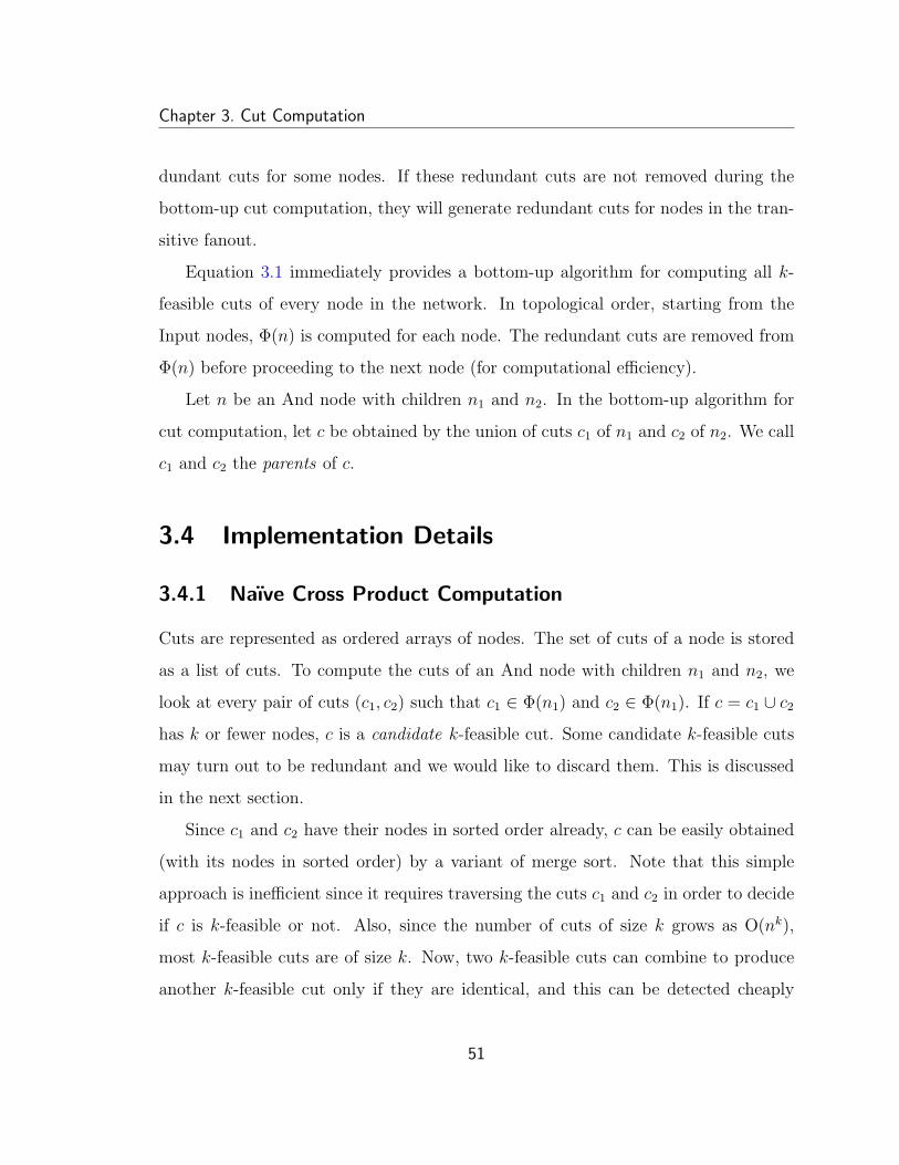
Chapter 3. Cut Computation
dundant cuts for some nodes. If these redundant cuts are not removed during the
bottom-up cut computation, they will generate redundant cuts for nodes in the tran-
sitive fanout.
Equation 3.1 immediately provides a bottom-up algorithm for computing all k-
feasible cuts of every node in the network. In topological order, starting from the
Input nodes, Φ(n) is computed for each node. The redundant cuts are removed from
Φ(n) before proceeding to the next node (for computational efficiency).
Let n be an And node with children n1 and n2. In the bottom-up algorithm for
cut computation, let c be obtained by the union of cuts c1 of n1 and c2 of n2. We call
c1 and c2 the parents of c.
3.4 Implementation Details
3.4.1 Naıve Cross Product Computation
Cuts are represented as ordered arrays of nodes. The set of cuts of a node is stored
as a list of cuts. To compute the cuts of an And node with children n1 and n2, we
look at every pair of cuts (c1, c2) such that c1 ∈ Φ(n1) and c2 ∈ Φ(n1). If c = c1 ∪ c2
has k or fewer nodes, c is a candidate k-feasible cut. Some candidate k-feasible cuts
may turn out to be redundant and we would like to discard them. This is discussed
in the next section.
Since c1 and c2 have their nodes in sorted order already, c can be easily obtained
(with its nodes in sorted order) by a variant of merge sort. Note that this simple
approach is inefficient since it requires traversing the cuts c1 and c2 in order to decide
if c is k-feasible or not. Also, since the number of cuts of size k grows as O(nk),
most k-feasible cuts are of size k. Now, two k-feasible cuts can combine to produce
another k-feasible cut only if they are identical, and this can be detected cheaply
51

Chapter 3. Cut Computation
using hashing.
3.4.2 Signatures
This brings us to the notion of signature of a cut. The signature of a cut is a hash
function defined as follows:
sign(c) =⊕n∈c
2id(n) mod M (3.2)
where we assume that every node in the aig has an unique integer id denoted by
id(n), and M is a constant equal to the word size of the machine (i.e. M = 32 on
a 32-bit machine). ⊕ denotes bit-wise or. Thus the signature of a cut is a machine
word with 1s in bit positions corresponding to the node ids (modulo M).
The signature is computed when the cut is constructed and stored with the cut.
Signatures can be computed incrementally since for a cut c = c1 ∪ c2, sign(c) =
sign(c1)⊕ sign(c2).
Example 3.2 Let M = 8 for ease of exposition. The cut c1 with nodes having ids
32, 68, and 69 has sign(c1) = 0011 00012. A second cut c2 with nodes having ids 32,
68, and 70 has sign(c2) = 0101 00012. A third cut c3 with nodes having ids 36, 64,
and 69 has sign(c3) = 0011 00012. Observe that c1 and c3 have the same signature
although they are different cuts. This is called aliasing.
Equality Check
To determine if two cuts c1 and c2 each of size k can produce a k-feasible cut, we first
compare sign(c1) and sign(c2). If they are different (the common case), then the cuts
have different nodes, and hence cannot produce a k-feasible cut. If the signatures
52

Chapter 3. Cut Computation
are the same (rare case), then we traverse both cuts to check k-feasibility. Thus
signatures allow a quick negative test of equality.
Example 3.3 In Example 3.2, since sign(c1) 6= sign(c2), we can immediately con-
clude that c1 6= c2). On the other hand, the fact sign(c1) = sign(c3) tells us nothing.
We have to do a node-by-node comparison to check if c1 and c3 are equal or not.
Size Check
Note that the number of bits set to 1 in the signature is a lower bound on the size
of the cut since each node sets exactly 1 bit to true in formula 3.2. This can be used
to filter out cut pairs (c1, c2) that cannot produce k-feasible cuts by computing the
number of bits set to 1 in sign(c1)⊕ sign(c2).
3.4.3 Removing Redundant Cuts
The cross product operation described above may produce some redundant cuts that
we would like to detect and discard. Given two cuts c1 and c2, if c1 ( c2 we say c1
dominates c2. Thus if a cut is dominated by another cut, it is redundant.
Signatures provide a quick negative test for domination. Given two cuts c1 and c2,
if sign(c1)⊕ sign(c2) 6= sign(c2), then c1 does not dominate c2. Otherwise, a detailed
check is needed.
During the cross product, each candidate cut is compared with all cuts that have
been generated so far. If the candidate cut dominates another cut, the dominated cut
is removed. If the candidate cut is dominated by another cut, then it is immediately
discarded.
Example 3.4 Continuing with Example 3.2, consider a fourth cut c4 with nodes
having ids 32, and 33. Therefore sign(c4) = 0000 00112, and sign(c4) ⊕ sign(c1) =
53

Chapter 3. Cut Computation
0011 00112. Since 0011 00112 6= sign(c1), we can conclude that c4 does not dominate
c1 without doing a detailed check.
3.4.4 Limiting the Number of Cuts
In spite of removing redundant cuts, it is sometimes necessary to set a hard limit on
the number of cuts considered at a node to keep the cut computation scalable. We
found a limit of 1000 cuts per node to be adequate for k = 6 in the sense that it was
rarely reached across a large set of benchmarks.
In this context, it is convenient to store the list of cuts of a node in order of
increasing size. During the cross product computation, pairs of cuts smaller than k
are tried first; then pairs of cuts where one cut is size k and the other smaller than k,
and finally pairs of cuts of size k are tried. During this process if the limit is reached,
the remaining pairs are not tried. The reason for this order is that most cuts of a
node are of size k, and if one cut of a pair being considered is of size k, then the other
cut of the pair must be contained in it for the resultant cut to be a candidate. This
is unlikely.
3.5 Cut Function Computation
3.5.1 Definition
Intuitively, the function of a cut c of a node m is the function of node m in terms of
the nodes in c.
Formally, let X1, X2, . . . , Xk be distinct Boolean variables. An assignment σc is a
map that assigns a Boolean variable Xi (1 ≤ i ≤ k) to each node in a k-feasible cut
c. Recall from Section 2.2.4 that each node in the aig has an unique integer id which
induces an order on the nodes of the aig. This allows us to view a cut as an ordered
54

Chapter 3. Cut Computation
set of nodes. An assignment is standard if the first node in the cut maps to X1, the
second node to X2 and so on.
The function of a cut c of node m under an assignment σ, denoted by πσ(m, c)
is the Boolean function of m according to the aig under the assignment (in terms of
the Xi). In what follows, if we do not specify an assignment for a cut function, the
standard assignment should be assumed.
Note that the function of a trivial cut under the standard assignment is always
X1.
Example 3.5 In the aig of Figure 3.1, let the node ids be assigned in alphabetical
order, i.e.
id(a) < id(b) < id(c) < · · · < id(x)
Consider the cut c1 = {b, c} of e. Let σ1 be the standard assignment, i.e. σ1(b) =
X1 and σ1(c) = X2. Therefore,
πσ1(e, c1) = ¬X1 · X2
i.e. the function of cut c1 of e is ¬X1 · X2.
Let σ′1 be the (non-standard) assignment defined by σ′
1(b) = X2 and σ′1(c) = X1.
Therefore,
πσ′1(e, c1) = ¬X2 · X1
Example 3.6 As a more complicated example, consider once again the aig in Fig-
ure 3.1 with the same ordering of the nodes as in Example 3.5. Consider the cut
c2 = {a, b, e} of node f . Let σ2 be the standard assignment i.e. σ2(a) = X1,
σ2(b) = X2, and σ2(e) = X3. Therefore,
πσ2(f, c2) = ¬(X1 · X2 + X3)
55

Chapter 3. Cut Computation
The subtlety here is that in the aig node b is an input of node e. They are not
independent since when b is 1, e must be 0. Nevertheless, we assign independent
variables X2 and X3 to b and e respectively, and ignore the edge connecting the two
nodes when evaluating the function of the cut. Thus the cut function is in some
sense over-defined since we are not using the satisfiability don’t cares inherent in the
structure of the aig.
3.5.2 Function Computation
In function computation, the goal is to compute the functions of each cut under the
standard assignment. For small values of k, truth tables are a convenient representa-
tion of the cut functions. Usually, k ≤ 6 for standard cell mapping and fpgas, and
so the cut functions can be represented by two machine words on a 32-bit machine.
The naıve method to compute the cut function follows from the definition above.
The formal variables X1, X2, X3, . . . , Xk are represented by truth tables (bit-strings of
length 2k) as follows:
X1 7→ 0101 0101 · · · 0101 0101
X2 7→ 0011 0011 · · · 0011 0011
X3 7→ 0000 1111 · · · 0000 1111...
Xk 7→ 0000 0000 · · · 1111 1111
A truth table is computed for each node in the volume of the cut in topological
order as follows. First, each node in the cut is associated with the truth table of the
corresponding formal variable under the standard assignment. The truth table of an
And node in the volume of the cut is computed by bit-wise and and negation from
the truth tables of its input nodes. In this manner the cut function is built from the
leaves up towards the node.
56

Chapter 3. Cut Computation
In practice, we use a recursive procedure that starts from the node, and computes
the function of the node from the function of its inputs. The base cases of the recursion
are the nodes in the cut whose functions are X1, X2, . . . Xk.
Example 3.7 Recall the Examples 3.5 and 3.6 of Section 3.5.1 where we computed
the functions for a few cuts under different assignments. Those functions would be
represented as follows:
Function Representation
πσ1(e, c1) = ¬X1 · X2 0010 0010 · · · 0010 0010
πσ′1(e, c1) = ¬X2 · X1 0100 0100 · · · 0100 0100
πσ2(e, c2) = ¬(X1 · X2 + X3) 1110 0000 · · · 1110 0000
Note that the naıve method requires traversing a part of the aig to determine
the function of a cut. In order to compute the functions for all the cuts, this method
is inefficient since it may process the same part of the aig many times. A second
problem arises in conjunction with choices and is discussed in Section 3.6.4.
3.5.3 Incremental Computation
The redundant computation of the naıve method can be avoided by computing the
function of a non-trivial cut from the functions of its parents. This allows the cut
function to be computed as the cut is constructed during the bottom-up procedure.
We begin with two examples from Figure 3.1. As before, node ids are assumed to be
in alphabetical order.
Example 3.8 Consider the construction of cut cd = {a, b} of node d from its parents
ca = {a} of node a and cb = {b} of node b. From the aig, the function of cd under
the standard assignment σ is,
πσ(d, cd) = πσ(a, ca) · πσ(b, cb)
57

Chapter 3. Cut Computation
The naıve method would compute πσ(a, ca) and πσ(b, cb) from scratch by traversing
the aig. In incremental computation we wish to avoid this traversal by computing
πσ(a, ca) and πσ(b, cb) from the previously computed functions of ca and cb respectively.
Let σ1 be the standard assignment for ca. In the incremental setting we have
already computed the function of ca, i.e. πσ1(a, ca). We want to use πσ1(a, ca) to
compute πσ(a, ca). This is easy, since under both σ and σ1, the node a is mapped to
the same formal variable (X1). Therefore,
πσ(a, ca) = X1 = πσ1(a, ca)
In the case of cb, the situation is more complicated. Let σ2 be the standard
assignment for cb. Under σ2, node b maps to X1, whereas, under σ, node b maps to
X2. Thus πσ(b, cb) = X2 but πσ1(b, cb) = X1. In this simple example, it is clear that
the desired function πσ(b, cb) is the same as the cut function πσ1(b, cb) except for a
substitution of variables, viz. X1 is replaced by X2.
Example 3.9 As a less trivial example, consider the construction of cut cf = {a, b, c}
of node f from its parents cd = {a, b} and ce = {b, c}. Let σ be the standard
assignment for the cut cf . From the aig it is clear that
πσ(f, cf ) = ¬πσ(d, cd) · ¬πσ(e, ce)
The functions of cuts cd and ce, however, are computed under their standard
assignments: σ1 for cd and σ2 for ce. Note that σ1 agrees with σ since σ1(a) = σ(a) =
X1 and σ1(b) = σ(b) = X2. Therefore one can check from the aig that,
πσ(d, cd) = X1 · X2 = πσ1(d, cd)
58

Chapter 3. Cut Computation
However, σ and σ2 disagree since, in particular, σ(b) = X2 whereas σ2(b) = X1.
Therefore, πσ(e, ce) 6= πσ2(e, ce). Indeed, from the aig it is easy to check that
πσ(e, ce) = ¬X2 · X3 and πσ2(e, ce) = ¬X1 · X2.
Once again, observe that the desired function πσ(e, ce) is the same as the cut
function πσ2(e, ce) except for a change of variables, viz. X1 is replaced by X2, and, X2
by X3.
More generally, let n be an And node with children n1 and n2. Let c be a cut of
n, c1 a cut of n1, and c2 a cut of n2 such that c1 and c2 are parents of c i.e. c = c1∪c2.
Let σ1 and σ2 be the standard assignments on c1 and c2 respectively. We are given the
functions π1 = πσ1(n1, c1) and π2 = πσ2(n2, c2), and asked to compute π = πσ(n, c).
From the above examples, it is clear that the main complication is due to the fact
that π1 and π2 are computed under assignments σ1 and σ2 which may differ from the
desired assignment σ for π. To rectify this, we need to re-express π1 and π2 in terms
of the assignment σ corresponding to π. Call these π′1 and π′
2, i.e. π′1 = πσ(n1, c1)
and π′2 = πσ(n2, c2).
The algorithm to compute π given the cuts c, c1 and c2 is shown in Listing 3.1. It
begins by computing π′1 by iterating over the nodes of c1. For a node m, the Boolean
variable σ1(m) is replaced by the Boolean variable σ(m) using Shannon decomposi-
tion. The only subtlety is that the last variable (i.e. the variable corresponding to
the node with highest id) under the assignment σ1 is replaced first, the second last
variable next, and so on. (The π1 obtained at the end of this iteration is π′1, the
function of node n1 in terms of the cut c1 under the assignment σ.) Similarly, the
next loop computes π′2.
Once π′1 and π′
2 are computed, it is straightforward to compute the function of
node n under the assignment σ.
59

Chapter 3. Cut Computation
Listing 3.1 incremental-cut-function(n, c, c1, c2)
Input: Cut c of node n with input edges (n1, i1) and (n2, i2); cut c1 of n1 and cut c2
of n2 where c = c1 ∪ c2
Output: The cut function π of c
Let π1 be the function of c1 and σ1 the standard assignment of c1
for each node m in c1 in descending order by id do
assert σ1(m) = σ(m) or π1 is independent of σ(m)
π+ ← pos cofactor of π1 w.r.t. σ1(m)π− ← neg cofactor of π1 w.r.t. σ1(m)π1 ← σ(m) · π+ + ¬σ(m) · π−
end for
Let π2 be the function of c2 and σ2 the standard assignment of c2
for each node m in c2 in descending order by id do
assert σ2(m) = σ(m) or π2 is independent of σ(m)
π+ ← pos cofactor of π2 w.r.t. σ2(m)π− ← neg cofactor of π2 w.r.t. σ2(m)π2 ← σ(m) · π+ + ¬σ(m) · π−
end for
if (i1 = 1) then π1 ← ¬π1 endifif (i2 = 1) then π2 ← ¬π2 endif
π ← π1 · π2
60

Chapter 3. Cut Computation
3.6 Cut Computation with Choices
3.6.1 Overview
In this section we extend cut computation to an aig with choice (G,',X ). An aig
with choice may be seen as a compact encoding of a set G of aigs (without choice).
Now pick a particular aig H ∈ G and compute k-feasible cuts for each node in H.
Imagine collecting all cuts for a node n ∈ G from all the individual cut computations
over the elements in G. Intuitively, this corresponds to the set of cuts of n in the aig
with choice. In this section, we show how this set of cuts can be computed directly
from the aig with choice without explicitly generating G.
3.6.2 Algorithm
Let G = (G,',X ) be an aig with choice such that the relation (Section 2.5.4)
does not have a cycle. Let X be the set of nodes of aig G. We compute cuts for
both equivalence classes in X' and nodes in X by modifying (3.1). The set of cuts
for an equivalence class N ∈ X' is
Φ'(N) =⋃n∈N
Φ(n) (3.3)
If n is an And node, let N1 and N2 be the equivalence classes of its inputs. Then we
define
Φ(n) =
{{n}} : n is an Input node
{{n}} ∪ (Φ'(N1) ./ Φ'(N2)) : n ∈ X and n is an And node
Φ'(N1) ./ Φ'(N2) : otherwise
(3.4)
61

Chapter 3. Cut Computation
Note that the trivial cut is added only for nodes that are representatives.3 This is
because only one trivial cut is needed for an equivalence class. A consequence of this
is that only representative nodes may belong to a cut.
The acyclicity of the relation is necessary for the mutually recursive definitions
of Φ(n) and Φ'(n) to be valid. To compute Φ(n) for every node n in G, we first
fix a topological order on the nodes according to the relation using a depth-first
traversal. Next, we process every node n in this topological order, and use (3.4)
to compute its set of cuts. If n is a representative of an equivalence class N , then
we compute Φ'(N) according to (3.3), and store it at n. Note that at this point
Φ(m) has been computed for all nodes m ∈ N , since we are processing the nodes in
topological order by .
Example 3.10 As we saw in Example 2.4, every aig may be viewed as an aig with
choice where each equivalence class N has exactly one member n. In this case, the
reader can check that Φ(n) computed according to equations (3.3) and (3.4) is equal
to Φ(n) computed according to (3.1).
Example 3.11 Figure 3.2 shows the aig with choices from Example 2.5 annotated
with Φ(n) for every node for k = 4. We note that there are cuts that “cut across”
equivalence classes. For example, consider the cuts {a, p, s} and {a, q, r} of node o.
The first cut is due to a cut of u ({p, s}), whereas the second cut is due to a cut of t
({q, r}).
3.6.3 Implementation Details
When combining the cut sets of the nodes in an equivalence class, there may be
duplicates. Therefore, signatures can be used to detect and remove duplicates and
dominated cuts as described in Section 3.4.2.3Recall from Section 2.4.1 that Input nodes are assumed to be representatives.
62

Chapter 3. Cut Computation
Figure 3.2: An aig with choice annotated with Φ(n) for every node n for k = 4. Inthis aig, all equivalence classes other than {t, u} are trivial, and are of the form {n}and Φ'({n}) = Φ(n). Since Φ'({t, u}) = Φ(t) ∪ Φ(u), we have Φ(o) = {o} ∪ ({a} ./(Φ(t) ∪ Φ(u)).
Example 3.12 In Example 3.11, the set {b, c, d, e} is a cut of both nodes t and u.
Therefore, when the cuts sets of t and u are merged to construct Φ'({t, u}), this
duplication can be detected and eliminated.
We also note that once Φ'(N) is computed for an equivalence class N , there is
no further need to store Φ(n) for n ∈ N and this memory can be re-used. (In the
subsequent steps of the mapping procedure, we deal only with cuts of equivalence
classes.)
Furthermore, as discussed in Section 3.4.4, it is necessary to limit the number of
cuts at an equivalence class to keep the computation scalable.
63

Chapter 3. Cut Computation
3.6.4 Incremental Cut Function Computation
As seen in Example 3.11 a cut may “cross” an equivalence class. This adds to the
inefficiency of the naıve approach to cut function computation since additional infor-
mation has to be stored with a cut to pick the correct member of an equivalence class
during the recursive traversal described in Section 3.5.2.
On the other hand, the incremental function computation of Section 3.5.3 requires
little modification to handle choices. Recall that in the incremental function compu-
tation, the function of a cut c of an And node n is computed from functions of its
parent cuts c1 and c2. c1 and c2 are cuts of the input nodes n1 and n2 of n respectively.
In an aig with choice, the function of a cut c of node n is computed from its
parents c1 and c2 as before. It is possible, however, that c1 and c2 are not cuts of the
actual inputs n1 and n2 of n, but are cuts of nodes n′1 and n′2 that are only functionally
equivalent up to complementation with n1 and n2. In particular, n1 and n′1 could be
complements of each other; similarly n2 and n′2.
Example 3.13 In Example 3.11, the parents of cut {a, p, s} of node o are the cut
{a} of node a and the cut {p, s} of node u. Although a is an input of node o, u is
not an input of o. Indeed, node u is the complement of t which is an input of o.
Therefore, when computing the function of a cut from its parents, we need to
possibly complement the cut function of the parent. In practice, this is done when
combining the cut sets of the members of an equivalence class N . Let r be the
representative of N . If n ∈ N and f(n) = ¬f(r) (f is the valuation function from
Section 2.2.2), then we invert the functions of the cuts of n when adding the cuts to
Φ'(N).
Example 3.14 In Example 3.11, suppose the node ids are ordered alphabetically
with the exception of o. o has the highest id. The function of cut {p, s} of u is
64

Chapter 3. Cut Computation
X1 ·¬X2. Since t is the representative of {t, u}, and f(u) = ¬f(t), when adding {p, s}
to Φ'({t, u}), we invert its function to get the new function ¬(X1 · ¬X2).
To compute the function of cut {a, p, s} of o, from the function of cut {a} (of the
equivalence class {a}) and cut {p, s} (of the equivalence class {t, u}), we first express
the new function of {p, s} in the standard assignment of {a, p, s} to get ¬(X2 · ¬X3).
The function of cut {a} in the standard assignment of {a, p, s} is X1. Now, as before,
we combine these functions to obtain the function ¬X1 · ¬(X2 · ¬X3) as the function
of {a, p, s} of o.
Compare this with the construction of cut {a, q, r} of o from cuts {a} (of the
equivalence class {a}) and {q, r} (of the equivalence class {t, u}). Since {q, r} is a
cut of t which is also the representative, we do not invert the function of {q, r} when
adding it to Φ'({t, u}). Thus the function of {q, r} remains ¬X1 · ¬X2. Expressing
this in the standard assignment of {a, q, r}, the function obtained is ¬X2 · ¬X3. Thus
we obtain the function ¬X1 · ¬X2 · ¬X3 as the function of {a, q, r}.
3.7 Related Work
The basic cut enumeration procedure we use (Section 3.3) is based on the simple
algorithm proposed by Pan and Lin [PL98] which was a significant improvement on
the previous algorithm based on spanning trees [CD93]. Our contribution here is the
efficient detection and removal of redundant cuts during the cut computation using
signatures (Section 3.4.2). Conceptually, the use of signatures is similar to the use
of Bloom filters for encoding sets [Blo70] and to the use of signatures for comparing
cnf clauses for subsumption in the context of sat solving [EB05].
The previous work on standard cell mapping using Boolean matching did not use
cuts, but instead relied on computing clusters [MM90; SSBSV92]. Clusters are like
cuts in that they correspond to single-output sub-graphs of the subject graph, and are
65

Chapter 3. Cut Computation
represented by their input nodes. Clusters of a node r are enumerated in a top-down
fashion starting with the trivial cluster containing only r. New clusters are obtained
by expanding existing clusters. Expansion is done by removing an input node of the
cluster and adding its fanins to the cluster. If in this process an existing cluster is
obtained, or the number of inputs exceeds a limit k, then the expanded cluster is
simply discarded.
Thus clusters of a node r computed with a limit of k input nodes form a subset
of the set of k-feasible cuts of r (i.e. every cluster is a cut). However, the top-down
approach means that certain deep k-feasible cuts of r may be missed if the circuit is
re-convergent. Indeed, such cuts may be the best kind for mapping since they are
deep and absorb reconvergences.
The use of the cut-based approach for standard cell mapping motivated the need
for efficient cut function computation described in Section 3.5. In fpga mapping,
cut function computation need not be efficient since only the functions of the cuts
that are finally selected in the mapped network need to be computed. However, for
Boolean matching in standard cells, the functions of all the cuts are needed.
Finally, we point out some recent attempts at improving cut computation by
reducing the resources required for enumeration. The work on factor cuts provides
a technique to avoid full cut enumeration by combining bottom-up cut computation
with top-down expansion [CMB06a]. The work on priority cuts takes this idea further
where only a few cuts are computed during mapping [MCCB07]. A different approach
is taken with bddcut where bdds are used to store cuts [LZB07]. This reduces the
memory required for storing cuts by sharing common subcuts. The main benefits of
these three approaches are obtained for large values of k (say 8 or larger). So far, the
use of these improved cut enumeration ideas has been mainly for lut-based fpga
mapping for large luts. Adapting these ideas to standard cell mapping or mapping
of macrocells in fpgas which more constrained than fpga mapping appears to be
66

Chapter 3. Cut Computation
an interesting problem.
67

Chapter 4
Boolean Matching and Supergates
4.1 Overview
In this chapter we present our simplified Boolean matching algorithm to match k-
feasible cuts with library gates for standard cell mapping.1 To the reader familiar
with Boolean matching algorithms, the simplified algorithm presented here may ap-
pear unorthodox: Rather than use NPN -canonization, we enumerate configurations
which are essentially different Boolean functions that a library gate can realize under
permutations and negations. To address the reader’s atavistic fear of enumeration,
we summarize certain advantages of the proposed method:
1. Since most gates used in standard cells mapping usually have a few inputs (say
6 or less),2 matching based on enumeration is faster than canonization. The
reason for this is described in Section 4.8.
2. Enumeration of configurations is easier to implement than canonization.
1No such technique is needed for fpgas since a k-lut can implement any k-feasible cut.2There are very few gates used in practice that have more than 6 inputs; these are typically
multiplexers (e.g. 8 to 1 mux) and are usually handled by specialized structural techniques whichsuffer from local structural bias.
68

Chapter 4. Boolean Matching and Supergates
3. This way of looking at the matching problem makes the concept of supergates
a natural extension for increasing the set of matches.
We begin with a few preliminary remarks and definitions relating to standard
cell libraries and gates (Sections 4.2 and 4.3). Then, we first look at a simplified
matching problem using p-configurations where we ignore inversions (Section 4.4).
Next, we introduce np-configurations which generalize p-configurations, and show
how np-configurations lead to more matches (Section 4.5). Finally, we introduce
supergates as a generalization of np-configurations and show how they can further
increase the number of matches (Section 4.6). We also briefly describe the connection
between supergates and choices (Section 4.7).
We postpone the detailed discussion of related work in the literature to the end
of the chapter (Section 4.8).
4.2 Preliminary Remarks
In standard cell designs, the combinational logic is implemented by gates that have
fixed functions. Thus we have a library of different gate types such as inv (inverter),
nand2 (two input nand gate), and3 (three input and gate), mux41 (4-1 multi-
plexer), etc. Typically each type of gate is actually a family of gates with different
electrical properties and timing characteristics. For instance there may be several dif-
ferent and3 type gates with different drive strengths, and different skews (i.e. input
pin to output pin delay characteristics).
For the purposes of matching, only the (logical) functionality of the gate matters
and not its electrical and timing characteristics. Therefore, as a first step we group
gates into functional families. This is described in more detail in Section 4.3.3.
The gates commonly used in practice to implement combinational logic have 6 or
fewer inputs. The Boolean matching technique described in this chapter is particu-
69

Chapter 4. Boolean Matching and Supergates
larly well-suited for matching such gates. For gates with substantially more inputs,
the method considered here is inadequate. Furthermore, the gates used to implement
combinational logic usually have only one output. Multi-output gates for combina-
tional logic are rare except for an important case: half-adder cells. These are typically
used on data-path circuits such as adders and multipliers. The method considered
here may be extended to handle such cells, but in what follows we restrict our atten-
tion to single-output gates.
4.3 The Function of a Gate
4.3.1 Functional Expression
The functionality of a (single-output) gate g is typically provided by an expression3 in
terms of its input pins, called the functional expression of g and denoted by expr(g).
For instance, for an nand2 with input pins a and b, could have expr(g) equal to
not(and(a, b)). An aoi21 gate (a three input And-Or-Invert gate) with inputs a, b
and c may have expr(g) equal to not(or(and(a, b), c)).
Formally, we assume that the functional expression of a gate g is generated by a
grammar such as:
<expr> ::= p | not(<expr>) | and(<expr>, <expr>) | or(<expr>, <expr>)
where p ranges over the names of the input pins of g. Now, if µ is a function that
maps the name of each input pin p of g to a Boolean function µ(p), then we define
3We distinguish expressions from functions here for reasons that will shortly become clear.
70

Chapter 4. Boolean Matching and Supergates
the function of an expression e under µ, denoted by π(e, µ) as follows:
π(p, µ) = µ(p)
π(not(e), µ) = ¬π(e, µ)
π(and(e1, e2), µ) = π(e1, µ) · π(e2, µ)
π(or(e1, e2), µ) = π(e1, µ) + π(e2, µ)
We shall use this general notion of the function of an expression under a map µ to
define the functions of different structures associated with gates.
4.3.2 Function under Assignment
The function of a gate g is defined in a manner analogous to that of the function of
a cut (Section 3.5.1). Suppose g has k inputs. Let X1, X2, . . . , Xk be distinct Boolean
variables. An assignment σ is a bijective map that assigns a Boolean variable Xi
(1 ≤ i ≤ k) to each input pin of a gate. The function of a gate g under the assignment
σ, denoted by πσ(g), is simply π(expr(g), σ).
Example 4.1 Let g be the nand2 gate with inputs a and b, and expr(g) = not(and(a,
b)). Let σ1 be the assignment that maps a to X1 and b to X2. Therefore,
πσ1(g) = ¬(X1 · X2)
Under a different assignment σ2 that maps a to X2 and b to X1, we have,
πσ2(g) = ¬(X2 · X1)
In the above example, we obtained the same function for both assignments σ1
and σ2 due to the symmetry of the nand2 gate. This is not true in general as the
following example shows.
71

Chapter 4. Boolean Matching and Supergates
Example 4.2 Let h be the aoi21 gate with inputs a, b and c, and expr(h) =
not(or(and(a, b), c)). Let σ1 be the assignment that maps a to X1, b to X2 and
c to X3. Therefore,
πσ1(h) = ¬((X1 · X2) + X3)
Under a different assignment σ2 that maps a to X2, b to X3 and c to X1, we have,
πσ2(h) = ¬((X2 · X3) + X1)
Now, πσ2(h) 6= πσ1(h).
As the above example shows, the function of a gate is not unique: it depends
on the assignment. (This is why we distinguished the function of a gate from the
expression.) This is similar to the function of a cut which is also not unique but
depends on the assignment used.
4.3.3 Implementation Details
In the implementation, the gates are read in from a library file. The functional
expression of a gate is parsed to get the abstract syntax tree (AST) of the expression.
The function of a gate under a specific assignment is obtained directly from the AST.
Functions are represented by truth tables as in the case of cuts (Section 3.5.2).
There may be multiple gates with the same functionality, but different timing
properties. The matching process is more efficient if such gates are collected to-
gether into functional families and only one member per functional family is used for
matching. Later, during match selection when the timing properties are important,
the different members of a functional family are considered.
An easy way to automatically detect such functional families is to compute the
function of the gates under a standard assignment that maps the first input of the
72

Chapter 4. Boolean Matching and Supergates
Figure 4.1: The aig for Example 4.3.
gate to X1, the second to X2 and so on. Gates that have the same function under the
standard assignment can be grouped together into a functional family.
4.4 Matching Under Permutations
4.4.1 Motivation
The Boolean Matching problem for standard cells asks if a cut c can be implemented
with a gate g. Let f be the function of c under the standard assignment. We could
use the standard assignment σg for g (as defined above) to check for a match. Now,
if πσg(g) = f , then clearly c can be implemented with g. However, by restricting
ourselves to a particular assignment for g, we may not detect a possible match. The
following example illustrates this.
Example 4.3 Consider the cut c = {p, q, r} of node t in the aig of Figure 4.1. The
node ids are in alphabetical order. Let σc be the standard assignment on c. Thus we
have,
πσc(t, c) = ¬X1 · ¬(X2 · X3)
Let h be the aoi21 gate from Example 4.2. Under the assignment that maps the i-th
73

Chapter 4. Boolean Matching and Supergates
input to Xi, i.e. the assignment σ1, we have
πσ1(h) = ¬((X1 · X2) + X3)
Thus g does not match c under this assignment. However, under the assignment σ2,
g matches c, since we have,
πσ2(h) = ¬((X2 · X3) + X1) = πσc(t, c)
Therefore, we cannot restrict our attention to the standard assignment for a gate,
but need to consider multiple assignments. Formally, we say a gate g matches a cut
with function f , if there exists an assignment σ such that πσ(g) = f . We call this the
problem of matching under permutations.
4.4.2 p-configuration, p-match and Validity
If g is a gate, and σ an assignment, the pair (g, σ) is called a p-configuration. The
function of (g, σ) is defined as the function of g under σ. Note that two different p-
configurations p1 and p2 can have the same function, and they are called functionally
equivalent. Now, the problem of matching under permutations reduces to finding a
matching p-configuration.
Let fc be the function of cut c of node n in the aig. Let (g, σ) be a p-configuration
with function f . If f = fc, then the tuple (c, g, σ) is called a p-match for node n.
For convenience, we define a formal p-match called pi-match that only matches the
Input nodes of an aig.
We define the support of a p-match m = (c, g, σ) to be c (viewed as a set of nodes).
We define support(pi-match) to be the empty set. Now if a match m 6= pi-match
is to be used in a mapping, there must be p-matches for the nodes in support(m).
74

Chapter 4. Boolean Matching and Supergates
Listing 4.1 build-hash-table-p(L)
Input: Library of gates LOutput: Hash table H
for each gate g in L dofor each assignment σ of g do
f ← function of g under assignment σP ← lookup(H, f)insert(H, f,P ∪ {(g, σ)})
end forend for
This leads us to the notion of validity: A p-match m is valid if the set of p-matches
for each node n ∈ support(m) is non-empty.
4.4.3 Matching Algorithm
We solve the matching problem in a simple brute-force manner. We enumerate all
p-configurations corresponding to a gate, by enumerating all possible assignments of
the gate. Let g be a gate with k inputs. Since each assignment is a bijection from the
set of inputs of the gate to the set {X1, X2, ..Xk}, there are k! different assignments
(and therefore k! different p-configurations). Note that enumerating p-configurations
is feasible since we restrict ourselves to k ≤ 6.
The matching procedure is split into two sub-procedures build-hash-table-p
and find-p-matches. Procedure build-hash-table-p runs first and processes the
gates in the library L to construct a hash table H. H maps a function f to the set of
p-configurations whose function is f . The pseudocode is shown in Listing 4.1. Note
that this procedure is a pre-computation in the sense that it does not depend on the
aig being mapped. Also, note that the number of keys in H is quite small in practice
since many gates are symmetric and for a symmetric gate, multiple p-configurations
75
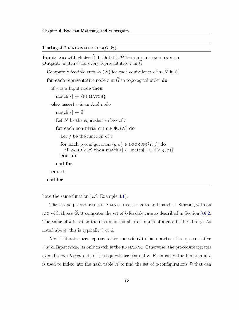
Chapter 4. Boolean Matching and Supergates
Listing 4.2 find-p-matches(G,H)
Input: aig with choice G, hash table H from build-hash-table-pOutput: match[r] for every representative r in G
Compute k-feasible cuts Φ'(N) for each equivalence class N in G
for each representative node r in G in topological order do
if r is a Input node then
match[r] ← {pi-match}
else assert r is an And node
match[r] ← ∅
Let N be the equivalence class of r
for each non-trivial cut c ∈ Φ'(N) do
Let f be the function of c
for each p-configuration (g, σ) ∈ lookup(H, f) doif valid(c, σ) then match[r] ← match[r] ∪ {(c, g, σ)}
end for
end for
end if
end for
have the same function (c.f. Example 4.1).
The second procedure find-p-matches uses H to find matches. Starting with an
aig with choice G, it computes the set of k-feasible cuts as described in Section 3.6.2.
The value of k is set to the maximum number of inputs of a gate in the library. As
noted above, this is typically 5 or 6.
Next it iterates over representative nodes in G to find matches. If a representative
r is an Input node, its only match is the pi-match. Otherwise, the procedure iterates
over the non-trivial cuts of the equivalence class of r. For a cut c, the function of c
is used to index into the hash table H to find the set of p-configurations P that can
76

Chapter 4. Boolean Matching and Supergates
be used to implement the cut. For each p-configuration (g, σ) ∈ P , it checks if the
p-match (c, g, σ) is valid. (Recall that a p-match is valid if every node in its support
has at least one p-match.) If the match is valid, it is added to the set of matches for
r. In this manner, the procedure constructs a list of matches for each representative
(and thereby each equivalence class) of G.
Remark As an important implementation detail, we note that memory used for
storing matches can be significantly reduced by not storing p-matches (as described
above) directly; instead, the same information can be represented by storing the pairs
(c,P).
4.4.4 Two Remarks on Matching Under Permutations
Remark 1 It would appear that a cut with k nodes can only match a gate with
k inputs. However, in practice it is possible that a cut c with k nodes matches a
p-configuration (g, σ) where g has less than k inputs. This happens with a badly
structured aig where the function of a cut does not depend on all k formal variables.
In particular, if the function is independent of the last variable Xk, a match may be
found with a gate with fewer than k variables.
The converse situation where a gate with k inputs matches a cut with less than k
nodes is also possible if there is a gate whose output expression does not involve all
of its input pins (such as tri-state elements). Such gates are usually excluded since
they cannot be meaningfully used by the matcher.
Remark 2 The single input gates (inverters and buffers) are never matched (except
in the degenerate case described in Remark 1) by procedure find-p-matches since
it does not consider trivial cuts. Therefore, the matching is not complete in the sense
that given a functionally complete library, there is no guarantee that a match will be
found for every node in the aig.
77

Chapter 4. Boolean Matching and Supergates
Figure 4.2: The aig for Example 4.4.
4.5 Matching Under Permutations and Negations
4.5.1 Motivation
Example 4.3 showed that by considering different assignments to the inputs of a
gate, we could detect more matches between cuts and gates. Different assignments
correspond to different input permutations of a gate. As the following example shows,
by considering input negations in addition to permutations, we can detect even more
matches.
Example 4.4 Figure 4.2 shows an aig similar to that of Example 4.3, except that
the arcs (p, t), (q, s) and (r, s) are complemented. Suppose our library contains an
inverter inv, and the aoi21 gate h as before. It is easy to see that h would not match
at cut c = {p, q, r} of node t under the assignment σ2 considered before. The function
of c under the standard assignment σc in this aig is
πσc(t, c) = X1 · ¬(¬X2 · ¬X3)
78

Chapter 4. Boolean Matching and Supergates
The function of aoi21 under assignment σ2 remains, as before,
πσ2(h) = ¬((X2 · X3) + X1)
Therefore, πσc(t, c) 6= πσc(t, c) in this example.
However, since we have an inverter, we could create a new gate i comprising the
aoi21 gate and an inverter at each input. The function of this new gate under the
assignment σ2, is
πσ2(i) = ¬((¬X2 · ¬X3) + ¬X1)
Now, πσ2(i) = πσc(t, c), and this new gate i matches the cut c.
Similarly, by adding an inverter to the output of an existing gate, we may find
more matches than otherwise.
The idea of creating new gates by combining gates in the library to improve
matching is a powerful one, and we shall explore it more fully in Section 4.6. However,
for now, we present a different method to achieve the same effect w.r.t. input and
output negations. Instead of creating gates by adding inverters to inputs or outputs,
we match each representative node of the aig in both positive and negative phases.
This is equivalent to matching edges of the aig instead of nodes.
Why do we prefer matching both phases over creating new gates with inverters?
We discuss this in Section 4.5.5 after the presentation of the matching algorithm.
4.5.2 np-configuration and np-match
Let g be a gate with k inputs, and σ an assignment for g. Let τ be a map that maps
an input pin of g to an element of {0, 1}. Informally, τ(i) = 1 means that input pin
i is inverted. The pair (σ, τ) is called a generalized assignment. Given a generalized
79

Chapter 4. Boolean Matching and Supergates
assignment (σ, τ), define the map µ on the input pins of g as follows:
µ(i) =
σ(i) if τ(i) = 0
¬σ(i) if τ(i) = 1
The function of a gate g under the generalized assignment (σ, τ) is defined to be
π(expr(g), µ).
Example 4.5 Let h be the aoi21 gate with inputs a, b and c, and expr(h) =
not(or(and(a, b), c)). Let σ = {a 7→ X2, b 7→ X3, c 7→ X1} and τ = {a 7→ 1, b 7→
0, c 7→ 1}. The function of h under the generalized assignment (σ, τ) is
π(σ,τ)(h) = ¬((¬X2 · X3) + ¬X1)
Example 4.6 Let i be an inverter with input a. expr(i) = not(a). There is only one
possible assignment for i which is σ = {a 7→ X1}. There are two possible τ maps:
τ1 = {a 7→ 0} or τ2 = {a 7→ 1} Thus we have two possible generalized assignments
with the following functions:
π(σ,τ1)(i) = ¬X1
and
π(σ,τ2)(i) = ¬¬X1 = X1
Similarly, a buffer b with input a, expr(b) = a, leads to two possible generalized
assignments:
π(σ,τ1)(b) = X1
and
π(σ,τ2)(b) = ¬X1
80
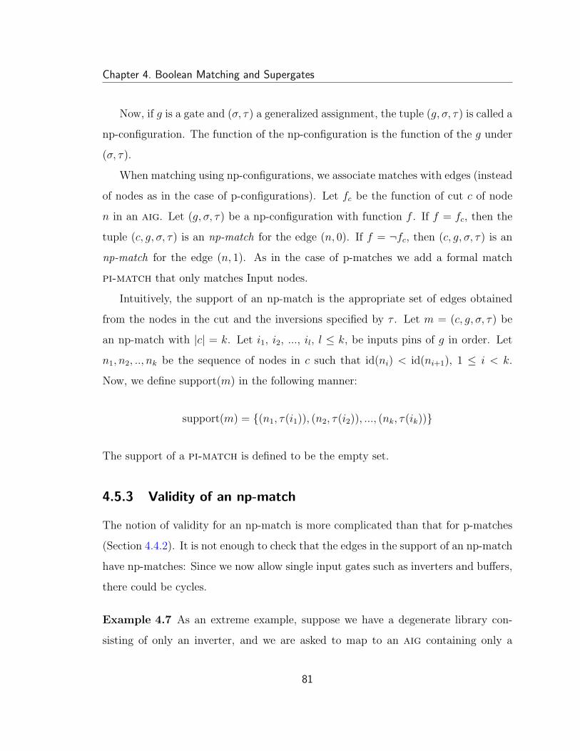
Chapter 4. Boolean Matching and Supergates
Now, if g is a gate and (σ, τ) a generalized assignment, the tuple (g, σ, τ) is called a
np-configuration. The function of the np-configuration is the function of the g under
(σ, τ).
When matching using np-configurations, we associate matches with edges (instead
of nodes as in the case of p-configurations). Let fc be the function of cut c of node
n in an aig. Let (g, σ, τ) be a np-configuration with function f . If f = fc, then the
tuple (c, g, σ, τ) is an np-match for the edge (n, 0). If f = ¬fc, then (c, g, σ, τ) is an
np-match for the edge (n, 1). As in the case of p-matches we add a formal match
pi-match that only matches Input nodes.
Intuitively, the support of an np-match is the appropriate set of edges obtained
from the nodes in the cut and the inversions specified by τ . Let m = (c, g, σ, τ) be
an np-match with |c| = k. Let i1, i2, ..., il, l ≤ k, be inputs pins of g in order. Let
n1, n2, .., nk be the sequence of nodes in c such that id(ni) < id(ni+1), 1 ≤ i < k.
Now, we define support(m) in the following manner:
support(m) = {(n1, τ(i1)), (n2, τ(i2)), ..., (nk, τ(ik))}
The support of a pi-match is defined to be the empty set.
4.5.3 Validity of an np-match
The notion of validity for an np-match is more complicated than that for p-matches
(Section 4.4.2). It is not enough to check that the edges in the support of an np-match
have np-matches: Since we now allow single input gates such as inverters and buffers,
there could be cycles.
Example 4.7 As an extreme example, suppose we have a degenerate library con-
sisting of only an inverter, and we are asked to map to an aig containing only a
81

Chapter 4. Boolean Matching and Supergates
single And node n (and its two input nodes). For the edge (n, 0), an inverter is the
only np-match. Call it m. It is easy to check that support(m) = {(n, 1)}. Now
for edge (n, 1), again, the only np-match is the inverter. Call this match m′. Now,
support(m′) = {(n, 1)}. In this case, although the edges in the support of both
np-matches also have matches, it is clear that a valid mapped network cannot be
constructed, since the matches m and m′ are mutually dependent, i.e. form a cycle.
To avoid such cycles stemming from mutually dependent matches due to single
input gates, it is convenient to divide np-matches into two groups: singular matches
and regular matches. Informally, singular matches are matches to single input gates
such as buffers and inverters. Regular matches are matches to multi-input gates and
pi-matches. To avoid cycles, we insist that for a singular match to be valid, the edge
in its support must have at least one regular match.
For a regular match to be valid, the edges in its support could have either regular
or singular matches. Either way, cycles would not be introduced. However, the
practical implementation can be greatly simplified by the following restriction. For
a regular match to be valid, the edges in its support must have singular matches.
Separately, we ensure that whenever, an edge has a regular match, it automatically
gets a singular match. This is done by adding a fake gate to the library called wire.
The gate wire is functionally a buffer, i.e. a single input, single output gate with
the identity function. As one might expect, the wire gate will be treated specially
during match selection (with regard to cost evaluation) since it is not a regular gate.4
Remark We want to emphasize that wire is added to simplify the implementation
of later operations of match selection, especially of match selection using exact area
(Section 6.7.2), rather than the matching procedure itself.5
4For e.g. wire transmits the load at the output pin to the input pin as opposed to, say, a buffergate. This distinction matters during match selection for load-based delay-oriented mapping.
5For this reason, wire is added to the library even when a buffer (which is functionally equivalent)
82

Chapter 4. Boolean Matching and Supergates
Listing 4.3 build-hash-table-np(L)
Input: Library of gates LOutput: Hash table H
Add special gate wire to L
for each gate g in L dofor each assignment σ of g do
for each phase assignment τ of g do
f ← function of g under generalized assignment (σ, τ)P ← lookup(H, f)insert(H, f,P ∪ {(g, σ, τ)})
end forend for
end for
Formally, pi-match is defined to be regular. An np-match (c, g, σ, τ) is regular
if |c| > 1 and is singular if |c| = 1. We base these definitions on the size of the cut
rather than number of inputs of the gate, due to the rare situation of a single-input
gate matching a non-trivial cut as described in Remark 1 of Section 4.4.4. A singular
match is valid if the edge in its support has at least one regular match. A regular
match is valid if the every edge in its support has at least one singular match.
4.5.4 Matching Algorithm
The matching algorithm is similar to that for matching under permutations: we gen-
erate all np-configurations of a gate. The procedure is split into two sub-procedures.
The first sub-procedure build-hash-table-np generates all np-configurations from
each gate in the library and constructs the hash table H of their functions. The
pseudocode is shown in Listing 4.3. Suppose g is a gate with k inputs. the num-
ber of np-configurations is k! · 2k. (Since, there are k! p-configurations, and each
already exists in the library.
83

Chapter 4. Boolean Matching and Supergates
Listing 4.4 find-matches-np(G,H)
Input: aig with choice G, hash table H from build-hash-table-npOutput: singular and regular matches for every representative r in G
Compute k-feasible cuts Φ'(N) for each equivalence class N in G
for each representative node r in G in topological order do
— compute regular matches —
if r is a Input node then
regular[(r, 0)] ← {pi-match}regular[(r, 1)] ← ∅ — no matches
else assert r is an And node
regular[(r, 0)], regular[(r, 1)] ← ∅
Let N be the equivalence class of r
for each non-trivial cut c ∈ Φ'(N) do
Let f be the function of c
for each np-configuration (g, σ, τ) ∈ lookup(H, f) doif valid(c, g, σ, τ) then regular[(r, 0)] ← regular[(r, 0)] ∪ {(c, g, σ, τ)}
end for
for each np-configuration (g, σ, τ) ∈ lookup(H, ¬f) doif valid(c, g, σ, τ) then regular[(r, 1)] ← regular[(r, 1)] ∪ {(c, g, σ, τ)}
end for
end for
end if
— compute singular matches —
singular[(r, 0)], singular[(r, 1)] ← ∅
for each np-configuration (g, σ, τ) ∈ lookup(H, X1) doif valid(c, g, σ, τ) then singular[(r, 0)] ← singular[(r, 0)] ∪ {({r}, g, σ, τ)}
end for
for each np-configuration (g, σ, τ) ∈ lookup(H, ¬X1) doif valid(c, g, σ, τ) then singular[(r, 1)] ← singular[(r, 1)] ∪ {({r}, g, σ, τ)}
end for
end for
84

Chapter 4. Boolean Matching and Supergates
p-configuration leads to 2k np-configurations, since the co-domain of the τ functions
is {0, 1}.) Since k ≤ 6, the maximum number of np-configurations is 720 · 64 = 46080
per gate. As noted before, the set of keys of H is smaller due to symmetries. We also
note that procedure build-hash-table-np adds the wire gate to the library.
The second procedure find-matches-np processes the cuts of the aig with
choices G to find matches using the hash table H computed by build-hash-table-
np. The pseudocode is shown in Listing 4.4. The first step is to compute all k-feasible
cuts of the equivalence classes as described in Section 3.6.2.
Next, for each representative r in G, the procedure first finds matching regular
np-configurations for each edge (r, 0) and (r, 1). If r is an Input node, then pi-match
is the only regular match for (r, 0), and there are no regular matches for (r, 1). If r
is an And node, then the matching regular np-configurations for each edge are found
by processing the non-trivial cuts. As in the case of matching under permutations,
only valid matches are stored.
After the regular np-matches have been computed, the procedure finds the singular
np-matches. Since an np-configuration of a single input gate can either be X1 or ¬X1
(Example 4.6), it uses those two functions to index into the hash table to obtain
singular np-matches. Again, only valid matches are stored.
To test his understanding of the matching algorithm, the reader may convince
himself that no singular np-match with a buffer or wire can be found for the edge
(r, 1) if r is an Input node.
4.5.5 Why Matching in Two Polarities is Better
Matching a node in both polarities is better than creating new gates from the library
gates by adding inverters (Section 4.5.1). The latter leads to duplicated logic in the
mapped circuit, as the following example shows:
85

Chapter 4. Boolean Matching and Supergates
Figure 4.3: The aig for Example 4.8.
Example 4.8 Consider the aig shown in Figure 4.3. Let the node ids be in alpha-
betical order. The function of cut cs = {p, q} of node s is X1 · ¬X2, and that of cut
ct = {q, r} of node t is ¬X1 · X2.
Suppose our library consists of an and2 gate g with inputs a and b, and an inverter
i with input a. It is easy to see that when matching under permutations we would
not find any matching p-configurations for nodes s and t. (The two p-configurations
of the and2 gate have the same function X1 · X2.)
However, we could construct a new gate h by adding the inverter to input a
of the and2 gate. The expression for h would be and(not(a), b). Let σ1 be the
assignment {a 7→ X1, b 7→ X2}. The function of the p-configuration (h, σ1) is ¬X1 ·X2
and therefore it is a match for cut ct. Indeed it is the only match for ct. The other
assignment σ2 = {a 7→ X2, b 7→ X1} of h has the function ¬X2 · X1. Therefore, it is
the (only) match for cs. Therefore, the aig can only be mapped with two instances
of h. Since each instance of h has an inverter, there are two inverters in the mapped
circuit. As may be verified, both inverters in the mapped circuit compute the same
function, and hence there is a redundancy.
In contrast when mapping under permutations and negations, gate i matches
edge (q, 1) under the generalized assignment ({a 7→ X1}, {a 7→ 0}). Let τ1 be the
map {a 7→ 1, b 7→ 0}. The generalized assignment (σ1, τ1) matches cut ct. Similarly,
if τ2 = {a 7→ 0, b 7→ 1} then the generalized assignment (σ2, τ2) matches cut cs. Now
86

Chapter 4. Boolean Matching and Supergates
in the mapped circuit, there is only one inverter.
Thus by mapping nodes in both polarities, we can avoid unnecessary duplication of
logic. Note that it is possible to avoid duplication by analyzing the mapped circuit for
redundancies. However, since cost estimates are incorrect during match selection, the
overall result is inferior (even after redundancies have been detected and eliminated).
We shall return to this subject again in Section 4.7.
4.6 Supergates
4.6.1 Motivation
We now return to the idea of combining library gates to form new gates in order to
find more matches. We call such gates constructed from other library gates super-
gates. Informally, a supergate is a single-output network of gates from the library.
In Example 4.4 we saw how simple supergates constructed by adding inverters to
the inputs and outputs of library gates can result in more matches being detected.
However, in that case, the same result can be obtained by mapping in both polar-
ities as discussed above. Therefore, we now present a more interesting example to
demonstrate the usefulness of supergates.
Example 4.9 Consider the aig shown in Figure 4.4 (I). Now, suppose we are given
a library consisting of an inv gate (inverter), and2 gate, a mux21 (2-1 multiplexer),
and an xnor2 gate and our task is to find all matches for every edge in the aig. Note
that the existence of the and2 gate and the inverter ensures functional completeness:
Procedure 4.4 will find matches for every edge.
Now consider the edge (v, 1) of the aig. Node v has a single cut of size 3, viz
{t, r, s}. It is easy to verify that no np-configuration of mux21 is a match for {t, r, s}.
87

Chapter 4. Boolean Matching and Supergates
Figure 4.4: Example illustrating how supergates can be used to find more matches. (I) Anaig where no np-configuration of a mux21 is a match for edge (v, 0). (II) A supergateconstructed from the mux21 and the xnor2 gate. (III) The result of mapping using thesupergate.
However, the mux21 can be matched by constructing a supergate. Consider the
supergate shown in Figure 4.4 (II) consisting of the mux21 fed by the xnor2 gate.
If we use a, b, and c to denote its input pins, we may describe the functional expression
of the supergate by the following expression:
or(and(not(a), not(xor(b, c))), and(a, c))
It is easy to verify that if the supergate were to be added to the library, then Proce-
dure 4.4 would match the supergate to the cut {t, r, s}.
Figure 4.4 (III) shows a mapping of the aig using the supergate and the and2
gate which matches the edge (t, 0). It provides an intuitive explanation for why the
mux21 cannot be directly matched to (v, 0). Consider the node x in the mapped
88

Chapter 4. Boolean Matching and Supergates
network. If a node with the same functionality were present in the aig, then the
mux21 match could have been found directly. Since that corresponding node does
not exist in the aig, a supergate is need to find the match.
This example illustrates the main idea behind supergates: Using bigger gates
allows the matching procedure to be less local, and thus less affected by the structure
of the aig. Furthermore, as this example illustrates, supergates are useful even with
standard cell libraries that are functionally rich.
4.6.2 Formal Definition
We are given a library of gates L. Let k be the largest number of inputs allowed for
a supergate (typically 6 or fewer).
4.6.2.1 Level-0 Supergates
Let X1, X2, .., Xk, be distinct Boolean variables. We define the set of all level-0 super-
gates S0 as follows:
S0 = {X1, X2, .., Xk,¬X1,¬X2, ..,¬Xk}
Note that we think of the Boolean variable Xi as a supergate. For convenience, we
define the function π(s) of a level-0 supergate s to be s itself, i.e. the function of X1
viewed as a level-0 supergate is X1.
4.6.2.2 Level-1 Supergates
Informally, a level-1 supergate is constructed by connecting level-0 supergates to the
inputs of a library gate. Formally, if g ∈ L is a gate with j inputs, j ≤ k, let ρ
be a bijective map from the input pins of g to S0. The pair (g, ρ) is called a level-1
89

Chapter 4. Boolean Matching and Supergates
supergate and g is called the root. The function of a level-1 supergate (g, ρ), is defined
to be π(expr(g), ρ) (Section 4.3.1). We abuse notation and use π(s) to denote the
function of a level-1 supergate s.
We use S1 to denote the set of all level-1 supergates that can be generated from
L and S0, i.e.
S1 = {(g, ρ) | g ∈ L and (g, ρ) is a level-1 supergate}
Note that the set S1 implicitly depends on L and k (through S0) and to be precise we
should incorporate this dependence into the notation. However, to keep the notation
simple, we omit L and k, trusting that they are clear from the context.
Example 4.10 Set k = 4. Let L consist of a single and2 gate g with input pins a
and b and expr(g) = and(a, b). Consider ρ = {a 7→ ¬X3, b 7→ X1}. Now, (g, ρ) is a
supergate and its function π((g, ρ)) is ¬X3 · X1.
In this case, S1 contains(82
)= 28 level-1 supergates, a few of which are degenerate.
For example, 4 supergates have the constant 0 function. They are of the type (g, {a 7→
Xi, b 7→ ¬Xi}).
Level-1 supergates are a generalization of np-configurations in the following sense:
If (g, σ, τ) is an np-configuration with function f , then there is a ρ s.t. the level-1
supergate (g, ρ) has function f . Proof: Pick ρ as follows:
ρ(i) =
¬σ(i) if τ(i) = 0
σ(i) if τ(i) = 1
However, not every level-1 supergate has a corresponding np-configuration with
the same function. If a gate g has j ≤ k inputs, then an assignment σ (in an np-
configuration) can only map an input pin p of g to a variable Xi where 1 ≤ i ≤ j. It
90

Chapter 4. Boolean Matching and Supergates
cannot map p to a Xi, j < i ≤ k. Thus there is no np-configuration with the same
function as the supergate of Example 4.10.
It is instructive to consider the reason for this difference between np-configurations
and level-1 supergates: The np-configurations are directly used to match with cuts.
Now since the variables assigned to a cut c of size j are Xi, 1 ≤ i ≤ j, np-configurations
are restricted likewise. In other words, generalizing np-configurations to use the
remaining variables would not result in more matches (except for the rare situation
described in Section 4.4.4).
On the other hand, level-1 supergates serve a second purpose beyond matching
cuts. They are used to build larger supergates. In this context, the more general
definition is useful since more logic structures can be explored, and a greater variety
of supergates can be constructed.
Example 4.11 In Example 4.9, suppose we are interested in all supergates having
3 or fewer inputs, i.e. k = 3. One of the level-1 supergates is s1 = (xnor2, ρ1) where
ρ1 = {a 7→ X2, b 7→ fa3}. This level-1 supergate does not match any cut in the aig,
but is used to build a level-2 supergate that does.
4.6.2.3 Level-2 Supergates
Let g ∈ L be a gate with j inputs. Let ρ be a bijective map from the input pins
of g to S0 ∪ S1. The pair (g, ρ) is called a level-2 supergate if (g, ρ) is not a level-1
supergate.6 The gate g is called the root of the supergate (g, ρ). Define the map µ on
the input pins of g as follows:
µ(i) = π(ρ(i))
The function of a level-2 supergate (g, ρ) is defined to be π(expr(g), µ) = π(expr(g), π◦
ρ). If s is a level-2 supergate, once again, we use π(s) to denote the function of s.
6i.e. for at least one input pin i of g, ρ(i) is a level-1 supergate
91

Chapter 4. Boolean Matching and Supergates
We use S2 to denote the set of all level-2 supergates that can be generated from L.
Example 4.12 The supergate comprising the mux21 and the xnor gate used in
Example 4.9 is a level-2 supergate s2 obtained by connecting the mux21 to the
level-1 supergate s1 obtained in Example 4.11. Formally, s2 = (mux21, ρ2) where
ρ2 = {s 7→ X1, d0 7→ s1, d1 7→ X3}. (The input pins of the mux21 are s, d0 and d1,
and the functional expression of the mux21 is or(and(not(s), d0), and(s, d1)).)
4.6.2.4 Level-n Supergates
Continuing in this way, if ρ is a bijective map from the input pins of g to⋃n−1
i=0 Si,
then (g, ρ) is called a level-n supergate if (g, ρ) is not a level-k supergate for any
k < n. The function of the supergate, denoted by, π((g, ρ)) is given by
π((g, ρ)) = π(expr(g), π ◦ ρ)
Once again, g is called the root of the supergate (g, ρ).
4.6.3 Generating Supergates
4.6.3.1 Overview
The formal definition of supergates immediately provides a representation for super-
gates in programs. The collection of all supergates is represented as a directed acyclic
graph (DAG), where each node represents a supergate. The leaf nodes in this DAG
are the level-0 supergates. In the first round, one iterates over each gate g in the
library, and constructs all level-1 supergates that can be constructed from g. Each
level-1 supergate thus obtained is represented by a new node in the DAG. In the
second round, one again iterates over each gate g in the library, and constructs all
level-2 supergates that can be constructed from g. Once again, each level-2 supergate
92

Chapter 4. Boolean Matching and Supergates
is represented by a new node in the DAG. In this manner, the set of supergates is
computed in a series of round until a user-specified amount of time elapses.
The adjacency information of the DAG of supergates is stored as follows: If node
s represents a supergate (g, ρ), and if g has j inputs x1, x2, .. xj, then there are exactly
j edges (ρ(xi), s), 1 ≤ i ≤ j in the DAG. These edges are represented by storing the
ρ(xi) at s.
4.6.3.2 Pruning
The number of supergates generated by the procedure described above is huge espe-
cially in modern libraries which contain hundreds of gates. Exhaustive generation of
supergates therefore is generally infeasible in mapping that uses a load-based model
of delay. However, if a constant-delay model is used for mapping7 then supergates
can be exhaustively generated for a few levels, provided some pruning is used. The
following example illustrates the need for pruning even if there are a few gates.
Example 4.13 Suppose during supergate generation, after level-1 supergates have
been computed there are 1000 supergates in all. Now, if the library contains a nand4
gate (i.e. a nand gate with 4 inputs), then there are roughly(1000
4
)possible level-2
supergates. In this case it would be impractical to enumerate all level-2 supergates
generated by the nand4 gate.
Therefore, during supergate generation, an attempt is made to reduce the number
of supergates considered through pruning. Pruning is of two types:
1. Pruning by Dominance. As we saw in Example 4.10, some supergates may
be degenerate and have the same function as a constant. During enumeration,
7This means that there are fewer gates in the library since gates with different drive-strengthsare represented with one gate.
93

Chapter 4. Boolean Matching and Supergates
we can detect these degenerate gates, and remove them from the set. This
prevents them from being used to build other supergates.
The idea of detecting and removing degenerate gates can be generalized by the
notion of dominance. Suppose during mapping we are interested in minimizing
two cost functions: delay and area. If we have two supergates s1 and s2 that
have the same function, such that
• the area of s1 is not (strictly) greater than the area of s2, and,
• the input to output delay of each input pin of s1 is not (strictly) greater
than that of the corresponding delay in s28
then we say that s1 dominates s2. Any mapping solution that uses s2 can be
improved in terms of area and delay by using s1 instead of s2.
Example 4.14 Suppose the library has an and2 gate with input pins a and b
and output z. Suppose the and2 gate has unit area, and that the delay from
a to z is 1 unit, and that from b to z is 2 units9. Now consider the supergates
si = (and2, ρi) defined as follows:
si ρi π(si)
s1 {a 7→ X1, b 7→ X2} X1 · X2
s2 {a 7→ X2, b 7→ X3} X2 · X3
s3 {a 7→ s1, b 7→ X3} (X1 · X2) · X3 = X1 · X2 · X3
s4 {a 7→ s1, b 7→ s2} (X1 · X2) · (X2 · X3) = X1 · X2 · X3
Now, the area of s3 is 2 units whereas that for s4 is 3 units. Furthermore, the
delays from input to output are as follows:
8We assume the constant-delay model here for simplicity.9We do not consider separate rise and fall delays here for simplicity.
94

Chapter 4. Boolean Matching and Supergates
Input Delay in s3 Delay in s4
X1 2 units 2 units
X2 3 units 3 units
X3 4 units 2 units
Thus s3 dominates s4.
To be complete, we point out here that two supergates obtained by permutation
need not dominate each other.
During supergate generation, we can detect all dominated gates by constructing
a hash table H indexed by the function of the supergate. When a new supergate
is constructed, we lookup in the hash table to find all supergates that have
the same function. If any existing supergate dominates the newly generated
supergate, then it is not added to the set of supergates. Otherwise, it is added
to the set of supergates, and also inserted into the hash table.
2. Pruning by Resource Limitations. A second method of pruning arises by
imposing artificial resource limitations on delay or area. For instance, only
supergates of a certain area or less are considered. Any supergate that exceeds
this limit is not added to the set of supergates (and hence does not participate
in the subsequent rounds).
A very useful resource limitation in practice is to set a limit n on the number
of inputs a root may have. Thus in each round after the first, only library gates
with n or fewer inputs are used to construct supergates. In practice n = 3 is
a reasonable limit, and even n = 2 leads to a good set of supergates. (Note
that this method of pruning directly prevents the combinatorial blow-up seen
in Example 4.13.)
95

Chapter 4. Boolean Matching and Supergates
4.6.4 Matching Using Supergates
A level-k supergate is called proper if k > 0. Only proper supergates are used for
matching i.e. level-0 supergates are not used for matching.
Proper supergates can be used in the matching process by a simple modification of
the process used to match regular library gates using np-configurations. First, a hash
table H is created which maps a Boolean function f to the set of proper supergates
whose function is f . This is similar to the hash table created by Procedure build-
hash-table-np (Listing 4.3) for np-configurations. Second, by a procedure similar to
Procedure find-matches-np (Listing 4.4) the cuts are matched with corresponding
supergates using H. In this context, the singular matches will be matches to the
level-1 supergates generated by inverters and buffers in the library.
Remark Note that we do not match to level-0 supergates since we exclude them from
the hash table H. This is because they do not correspond to real library gates, but
play a role similar to that of np-configurations to permit matching in both polarities
(Section 4.6.2.2). In particular, the level-0 supergate ¬X1 should be used to match
since it is possible the library might not have an inverter. (If the library has an
inverter then there will be a level-1 supergate with the function ¬X1. This supergate
will be used in matching.)
4.7 Supergates and Choices
Supergates can be seen as a technique for creating choices. Unlike the choices due to
algebraic rewriting or lossless synthesis, the choices introduced by supergates come
from the library. Thus, if a supergate matches at an edge r in an aig with choice G,
it is possible to create a new aig with choice G′ from G such that mapping without
supergates (i.e. using just np-configurations of library gates) on G′ leads to the match
96

Chapter 4. Boolean Matching and Supergates
Figure 4.5: Example illustrating how supergates lead to choices.
97

Chapter 4. Boolean Matching and Supergates
that was found using supergates.
Example 4.15 Figure 4.5 (I) reproduces the aig of Example 4.9, and Figure 4.5
(II) shows a mapped network M corresponding to the aig that uses the supergate
constructed in that example. Now consider an aig obtained from M by decomposing
its constituent library gates into two input and gates and inverters. This aig is
shown in Figure 4.5 (III). Note that the function of node v′ in (III) is the complement
of the function of node v in (I). Now, if the choice operator (Section 2.6) is used to
combine these two aigs to form a single aig with choice G′, we obtain the structure
shown in Figure 4.5 (IV) where nodes v and v′ belong to the same equivalence class,
say V .
Now, if mapping is performed on G′ using only np-configurations (i.e. without
using supergates) then we find that the mux21 is a match for class V since the cut
{s, t, x} ∈ Φ'(V ).
Remark 1 In the light of the above discussion, it is possible to see supergate match-
ing as a semi-technology dependent synthesis step – call it superchoicing – for adding
choices using library information. Although experiments indicate that superchoicing
leads to good results, the main problem is that too many choices are added due to
the large number of supergate matches.
Remark 2 Our experience indicates that supergates are mainly useful for delay-
oriented mapping. They tend to increase area since common logic between two su-
pergates is not correctly accounted for during the selection process. We saw the
reason for this in Section 4.5.5 for the special case of supergates constructed using
only inverters and library gates. An interesting line of research would be to explore
the use of superchoicing in reducing the area overhead of using supergates.
98

Chapter 4. Boolean Matching and Supergates
4.8 Related Work
4.8.1 On NPN -Canonization
Mailhot and De Micheli first proposed the use of Boolean matching (instead of struc-
tural matching) for technology mapping [MM90]. However, their method to detect
when a library gate matches a cut function10 is different from ours. It is instructive
to look at their method since it motivated much of the subsequent work on Boolean
matching.
Two Boolean functions are NPN -equivalent if one can be obtained from the
other by negation of output, permutations of inputs, or negations of inputs (or any
combination thereof). To decide if a cut matches a library gate, Mailhot and De
Micheli enumerate all functions that are NPN -equivalent to the cut function to see
if any one of them is equal to the11 function of the library gate. They also present
some heuristics to speed up the process by terminating this enumeration early.
In the terminology of this chapter, they essentially enumerate the different “np-
configurations” of a cut function12 to see which matches the function of a given library
gate. For each cut, this procedure is repeated for every library gate.
It is easy to see why this procedure is inefficient: It repeats the enumeration of
NPN -equivalent functions of each cut functions once for each library gate. Thus its
run-time is O(c · l) where c is the number of cuts and l is the number of gates in the
library. Furthermore, the constant hidden by the big-O notation is large. In contrast,
in our method, we pre-compute the different np-configurations of each library gate
once (an O(l) procedure with a large constant), and then each cut function just
requires two lookups in the hash table (an O(c) procedure with a small constant).
10In fact they used clusters instead of cuts (Section 3.7) but that difference is not important here.11In our terminology this would be the function of the gate under an arbitrary assignment.12Except they also consider the output negation which is not captured in the np-configuration.
We handle that by matching both the cut function and its complement.
99

Chapter 4. Boolean Matching and Supergates
Since c� l, our method is significantly faster.
Burch and Long improved upon Mailhot and De Micheli by proposing the use
of NPN -canonization [BL92]. Since NPN -equivalence is an equivalence relation, it
splits the set of all Boolean functions on k variables into equivalence classes. One
member of each class is designated as the representative of that class. Now, if we
have a procedure that given a function f returns the representative of the NPN -
equivalence class of f , then the following procedure can be used. First, we compute
the NPN -representative of the function of each library gate, and construct a hash
table of these representatives. Next, for each cut function, we compute the canonical
representative and look it up in the hash table to find a library gate that matches it.
However, the problem of finding the NPN -representative of a given function is
non-trivial, and much of the recent research in this area has addressed the problem of
making this efficient [CS03; DS04; AP05; CK06]. (In fact the problem of determining
canonical representatives is an old one [Gol59].13) However, we note that in the worst
case (for some classes of functions), all these methods lead to a search where different
NPN -equivalent functions are enumerated in order to find the representative. Thus,
although these methods can work with gates with more than 6 inputs, these methods
also have a limit. With current techniques this limit is around 12 inputs.
There are two main problems with the use of canonization in the context of tech-
nology mapping:
1. Every cut function needs to be canonized before the hash-table lookup, and this
is non-trivial. In contrast, in our method, there is no need to canonize. On the
other hand, in our method, the hash table contains more elements; but that
does not significantly increase the time for lookups.
2. After a match has been found, different symmetries of the function need to be
13We thank Donald Chai for this reference.
100

Chapter 4. Boolean Matching and Supergates
explored to find the different matches. (For instance, a multi-input And gate
will in general have different input pin to output delays; thus different matches
need to be explored.)
In summary, in the context of standard cell matching, our method is more efficient
and also simpler to implement than methods based on canonization.
On the other hand for matching problems where the number of inputs is larger
(say between 8–12), canonization-based methods are useful. However, note that in
such cases, it may be too expensive to actually evaluate the different matches during
selection. Also, exhaustive cut computation in such cases is not possible. For an
example of a mapping problem with these characteristics, see the work on factor
cuts [CMB06a].
We note here that the work on functional matching in the bddmap system is
similar to ours in that different permutations are enumerated [KDNG92]. However,
they use bdds instead of truth tables to represent functions. Thus, only those gates
which are highly symmetric or have a small number of inputs (say 3) are matched
using functional matching in order “to avoid possible exponential blowup of [bdds].”
All other gates are matched structurally. Somewhat paradoxically, by using truth
tables instead of bdds, we can use Boolean matching for a much larger class of gates.
The work on bddmap also addresses the question of mapping to both polarities
in the context of Boolean matching. However, they pick the solution of creating new
gates with inverters as described in Section 4.5.1. That method is inferior to our
method for reasons described in Section 4.5.5.
4.8.2 On Supergates
To our knowledge, the use of supergate-like constructs to increase the number of
matches has not been reported in the literature.
101

Chapter 4. Boolean Matching and Supergates
Hinsberger and Kolla consider increasing the set of possible matches by construct-
ing configurations from library gates [HK98]. These configurations are constructed
by bridging (i.e. connecting certain input pins together) or connecting constants to
certain inputs. Although the use of these configurations will increase the number of
matches, it is not clear what the benefit is. For instance, bridging inputs of a 4-input
and gate will lead to smaller and gates. However, in a realistic library, these smaller
and gates are likely to be present anyway, and the smaller gates will have better
area and delay compared to the larger gate with bridging. (In the absence of further
data, we must conclude that their improvements compared to sis stem from the use
of Boolean matching as opposed to the use of configurations.)
Note that in our framework, we can accommodate bridging by not requiring as-
signments to be bijective in Section 4.3.2. Setting some inputs to constants can
be accommodated by allowing level-0 supergates to also include the constant 0 and
constant 1 functions in Section 4.6.2.1.
The bottom-up supergate generation may be seen as an attempt at exact multi-
level synthesis for small functions. In this connection the reader may be interested
in some early work on exact multi-level synthesis of small functions using exhaustive
enumeration [Hel63; Dav69].
4.8.3 Supergates and Algebraic Choices
Recall from Section 2.7.2 that algebraic re-writing includes the addition of choices by
adding alternative decompositions based on associative and distributive transforms
in the manner of Lehman et al. [LWGH95].
The search space explored by supergates is different from the search space explored
by algebraic re-writing in two ways. First, since supergates are built by combining
gates, supergates capture different Boolean decompositions of a function. Therefore
102

Chapter 4. Boolean Matching and Supergates
they are more general than algebraic re-writing which by definition is limited to
algebraic decompositions. Second, since the set of decompositions explored depends
on the library, and the pruning techniques described above prune away sub-optimal
decompositions, supergates explore a space of “good” decompositions relative to the
gates in the library.
In summary, the decompositions due to supergates are a targeted – though sparse
– sampling of the large space of Boolean decompositions. In contrast, algebraic re-
writing is a dense sampling of the smaller space of algebraic decompositions.
103

Chapter 5
Match Selection for FPGA Mapping
5.1 Overview
In this chapter we look at the match selection problem in the context of fpga mapping
with a special focus on area-oriented selection. The goal of selection is to construct
the best mapped network by selecting a suitable set of matches. Although this chapter
deals only with fpga mapping, it may be of interest to the standard cell reader since
the main ideas behind the area-oriented selection algorithms are easier to grasp in
the simpler fpga setting.
We begin with a review of the cost models for fpga mapping (Section 5.2). Next,
we define the notion of a cover (Section 5.3). A cover identifies a subset of matches
that correspond to a valid mapped network, and in the rest of the chapter we deal
with mapped networks through covers. We begin our discussion of selection algo-
rithms with a generic selection procedure where the cost function is abstracted away
(Section 5.4). Then, we review depth-oriented selection in this context (Section 5.5).
Then, we present the main contribution of this chapter which is the area-oriented se-
lection algorithm for fpga mapping (Section 5.6). After that, we discuss briefly how
104

Chapter 5. Match Selection for FPGA Mapping
area and depth costs are used to break ties during selection (Section 5.7). Finally, we
look at how area-oriented selection may be combined with depth-oriented selection
to improve area under delay constraints (Section 5.8).
We postpone the detailed discussion of related work in the literature to the end
of the chapter (Section 5.9).
Notation Let G be an aig with choice, and let X be its set of representatives. Given
a node r ∈ X , we abuse notation and use Φ'(r) to denote Φ'(N) where N is the
equivalence class of r.
5.2 The Cost Model
Delay. We assume the commonly used unit delay model where each lut has constant
(unit) delay from any pin to output pin [CD96, Section 2.3]. The proposed algorithms
can also work with a non-unit delay model where the input-to-output delays are
different for different input pins of a lut. We point out the necessary modifications
at the appropriate place.
Area. We assume that the area of a lut depends on the actual function implemented
by the lut. We abstract this dependence away by assuming a function get-lut-
area that given a cut c returns the area required by a lut if it implements the
function of c.
For many fpga architectures such as Actel ProASIC III [Act07] (3-lut), Altera
Stratix [Alt06] (4-lut) and Xilinx Virtex [Xil07a] (4-lut) the area of a lut is inde-
pendent of the function implemented by it. In this cases, for any k-feasible cut c (k
depending on the architecture),
get-lut-area(c) = 1
105

Chapter 5. Match Selection for FPGA Mapping
For some newer architectures such as the Altera Stratix II [LAB+05] and Xilinx
Virtex-5 [Xil07b], a 6-input lut may be used to implement any Boolean function of
6 inputs or may be used to implement two Boolean functions of 5 inputs or fewer.
For these architectures, for a 6-feasible cut c we have,
get-lut-area(c) =
1 : if |c| ≤ 5
2 : if |c| = 6
5.3 Cover
Let G be an aig with choice. Intuitively, the set of k-feasible cuts for all equivalence
classes of G is an implicit description of a set of mapped networks. LetM denote this
set of mapped networks. The task of selection is to explicitly identify one mapped
network inM that is optimal w.r.t. the given cost function.
The notion of a cover is used to specify an arbitrary element M ∈ M. Let X be
the set of representatives of G. Let O be the set of output edges of G. Let ν be a
map that associates with every r ∈ X either a cut c ∈ Φ'(r) or the symbol nil. If
ν(r) 6= nil, then r is said to be selected in ν, and ν(r) is said to be the selected cut
of r, or simply the cut of r. The map ν is a cover if the following three conditions are
satisfied:
1. If (r, i) ∈ O then r is selected in ν.
2. If r is selected in ν then every r′ ∈ ν(r) is also selected in ν.
3. If r is selected in ν and r is an And node, then ν(r) is a non-trivial cut.
A cover ν is a complete description of a mapped network in the following manner:
For each representative r selected in ν, there is a net nr in the mapped network. If
r is an Input node, nr is driven by the input port corresponding to r in the mapped
106

Chapter 5. Match Selection for FPGA Mapping
network. Otherwise, nr is driven by a lut lr corresponding to r in the mapped
network. The configuration bits of lr are set according to the function of the cut ν(r).
The input pins of lr are connected to the nets corresponding to the representatives in
ν(r) (which by Condition 2 are also selected in ν).
The three conditions above ensure that the mapped network corresponding to a
cover ν is a valid one. Condition 1 ensures that there is a net corresponding to each
output in the mapped network. Condition 2 ensures that the input nets of a lut
are present in the mapped network. Condition 3 ensures that the trivial cuts are
only allowed for Input nodes (note that there are no luts corresponding to the input
nodes); all other representatives are implemented in the mapped network with luts.
To summarize, a cover is a complete description of a mapped network. In the
subsequent discussion, we shall deal with mapped networks though covers. The goal
of selection now becomes to select the optimal cover from among the possible covers.
5.4 Overview of the Selection Procedure
In this section we present an overview of the selection algorithm. For simplicity
of exposition, in this section, we do not deal with specific cost functions. The input
to the selection procedure is an aig with choices G. We assume that the set of cuts
Φ'(N) of each equivalence class N in G has already been constructed as described
in Section 3.6. The output of the selection procedure is a cover that optimizes the
given cost function.
The selection procedure is divided into two sub-procedures evaluate-matches
and cover. The sub-procedure evaluate-matches (Listing 5.1) is called first. It
processes the representative nodes in topological order starting from inputs. For each
representative r, it assigns the best1 non-trivial cut to best[r] and the corresponding
1according to the cost function abstracted here by the function eval-match-cost
107

Chapter 5. Match Selection for FPGA Mapping
Listing 5.1 evaluate-matches(G)
Input: aig with choice GOutput: best[r] for every And representative r in G
for each representative node r in G in topological order do
if r is a Input node then
cost[r] ← set-input-cost(r)best[r] ← {r}
else assert r is an And node
cost[r] ← minc∈Φ'(r)\{{r}}
eval-match-cost(c)
best[r] ← arg minc∈Φ'(r)\{{r}}
eval-match-cost(c)
end if
end for
Listing 5.2 cover(G, O, best[·])
Input: aig with choice G, set of output edges O, best[r] for each representative r
Output: nref[r] for every representative r in G
for each representative node r in G donref[r] ← 0
end for
for each edge (n, i) ∈ O donref[n] ← nref[n] + 1
end for
for each representative node r in G in reverse topological order do
if nref[r] > 0 and r is an And node then
for each n ∈ best[r] donref[n] ← nref[n] + 1
end for
end if
end for
108

Chapter 5. Match Selection for FPGA Mapping
cost to cost[r]. Although we defer the specification of the specific cost function to
later, one should think of the cost of a cut as a “cumulative” measure that includes
the cost of the subnetwork below it. Thus cost[r] is used by eval-match-cost
to determine the cost of cuts (of representatives in the transitive fanout of r) that
contain r. For now, also note that input nodes are treated specially.
Intuitively, evaluate-matches constructs part of the cover. For each represen-
tative r, best[r] stores the selected cut of r if r were to be selected in the cover. To
complete the construction of the cover, the sub-procedure cover is called next. The
pseudo-code of cover is shown in Listing 5.2. It constructs a cover in a straightfor-
ward manner by enforcing Conditions 1 and 2 of Section 5.3. (Condition 3 is enforced
by evaluate-matches.) Note that the procedure cover does not depend on the
cost function.
For each representative r, cover also computes nref[r] which is the number of
fanouts of the lut corresponding to r in the mapped network. (This fanout count
includes fanouts to output ports of the mapped network in addition to the fanouts
to other luts in the network.) The maps best[·] and nref[·] define a cover ν in the
following manner:
ν(r) =
best[r] : if nref[r] > 0
nil : otherwise
Finally, we remind the reader that only representative nodes in an aig with choice
may belong to a cut (Section 3.6.2). Therefore, the selection procedures evaluate-
matches and cover only deal with representative nodes.
5.5 Depth-Oriented Selection
In depth-oriented selection the goal is to choose a mapped network (or, equivalently,
a cover) with minimum depth i.e. minimum arrival time at the outputs. This is done
109

Chapter 5. Match Selection for FPGA Mapping
in the standard manner by choosing for each representative r a cut that minimizes
the arrival time.
Listing 5.3 evaluate-matches-depth(G)
Input: aig with choice GOutput: best[r] for every And representative r in G
for each representative node r in G in topological order do
if r is a Input node then
arrival[r] ← arrival time at input rbest[r] ← {r}
else assert r is an And node
arrival[r] ← minc∈Φ'(r)\{{r}}
arrival-time(c)
best[r] ← arg minc∈Φ'(r)\{{r}}
arrival-time(c)
end if
end for
As discussed in Section 5.4, depth-oriented selection is split into two sub-procedures.
Procedure evaluate-matches-depth is run first to select the best cut for each rep-
resentative r. Next, the cover procedure (Listing 5.2) is invoked to complete the
construction of the cover. As is well known in the literature, this procedure is optimal
i.e. produces a cover with minimum depth.
The pseudo-code for evaluate-matches-depth is shown in Listing 5.3. It is a
specialization of the generic evaluate-matches procedure shown in Listing 5.1 for
depth-oriented selection. For a representative r, arrival[r]2 is the minimum arrival
time possible for r. If r is an Input node, arrival[r] is set to the given arrival time for
that input. If r is an And node, arrival[r] is set to the minimum of the arrival times
from among the cuts of r. The arrival time of a cut c is computed in the unit delay
2arrival[r] corresponds to the generic cost[r] in Listing 5.1 in the context of depth-oriented map-ping
110

Chapter 5. Match Selection for FPGA Mapping
model (Section 5.2) as follows:
arrival-time(c) = 1 + maxr∈ c
arrival[r]
If the delays from input pins to output pin are different, then the arrival time of a
cut can be computed by assigning the input pin with smallest delay to output to the
latest arriving cut node, the input pin with second smallest delay to the second latest
arriving cut node, and so on.
5.6 Area-Oriented Selection
5.6.1 Overview
Area-oriented selection is done using two separate selection procedures which use
different heuristics to minimize area. The first area-oriented selection heuristic is
called area-flow. Area-flow is used to construct an initial cover with “good” area.
This cover is then greedily optimized by a second heuristic called exact area.
5.6.2 Area-Flow
Similar to depth-oriented selection, area-oriented mapping using the area-flow heuris-
tic is split into two sub-procedures. Procedure evaluate-matches-area-flow
runs first and assigns a best cut to each representative r. Next, procedure cover is
invoked which completes the construction of the cover.
The pseudocode for evaluate-matches-area-flow is shown in Listing 5.4.
For a representative r, area[r] measures the area (i.e. the cost) to implement r in the
mapped network. For an Input node r, area[r] is zero. For an And node r, area[r]
is the minimum area-flow cost among all cuts c of r. The area-flow cost of a cut c is
111

Chapter 5. Match Selection for FPGA Mapping
Listing 5.4 evaluate-matches-area-flow(G)
Input: aig with choice GOutput: best[r] for every And representative r in G
for each representative node r in G in topological order do
if r is a Input node then
area[r] ← 0best[r] ← {r}
else assert r is an And node
area[r] ← minc∈Φ'(r)\{{r}}
area-flow(c)
best[r] ← arg minc∈Φ'(r)\{{r}}
area-flow(c)
end if
end for
given by the following formula:
area-flow(c) = get-lut-area(c) +∑r∈ c
area[r]
fanouts(r)
where fanouts(r) is the number of fanouts of the representative r in the aig with choice
G. (Note that since r ∈ c, r fans out to at least one node. Therefore, fanouts(r) 6= 0.)
Intuitively, this definition of the area cost takes into account possible sharing at a
multi-fanout node. The cost of luts is distributed among the different fanouts. This
would be completely accurate if fanouts(r) would reflect the actual fanout of the lut
chosen for r in the mapped network. However, since the fanouts of r are mapped after
the best cut for r is selected, we simply estimate the fanout by assuming it to be the
same as that in the aig. This estimation is particularly inaccurate in the presence of
choices, since choices increase fanout.
Note that in the special case where G is a tree, and every equivalence class has
only one representative (i.e. G is an aig without choices), the area flow metric is the
112

Chapter 5. Match Selection for FPGA Mapping
same as area since fanouts(r) = 1 for all representatives r.
5.6.3 Exact Area
Unlike area-flow, exact area does not create a cover from scratch. Instead, it greedily
and incrementally optimizes an existing cover to increase sharing. The pseudocode for
the main exact area procedure improve-cover-exact-area is shown in Listing 5.5.
It invokes two auxiliary procedures recursive-select and recursive-deselect
whose pseudocode is presented in Listings 5.6 and 5.7.
Procedure recursive-select when invoked on a representative r is used to
compute the incremental area cost of selecting best[r] assuming that the rest of the
cover is fixed. The incremental area cost is the cost of selecting the luts that are
only used to implement best[r] (and not used anywhere else in the mapped network).
In other words this is the cost of the maximum fanout-free cone of r in the mapped
network. This cost is estimated by recursively selecting the best cuts for the nodes
in best[r] that are not currently selected. As a side effect of this routine, the nref[·]
array is updated to reflect the new fanout counts of the nodes after best[r] has been
selected.
Procedure recursive-deselect is the opposite of recursive-select. When
invoked on a representative r, recursive-deselect frees the luts that have been
selected exclusively to implement best[r]. Like recursive-select, it returns the
incremental area needed to select best[r]. As a side effect it updates nref[·] array to
reflect the new fanout counts of the nodes after best[r] has been de-selected.
The main improve-cover-exact-area procedure processes each representative
in topological order. For each representative And node r, it iterates through the non-
trivial cuts. If c is a non-trivial cut of r, it sets c to be the best cut of r, and
then invokes recursive-select to estimate the incremental cost of implementing
113

Chapter 5. Match Selection for FPGA Mapping
Listing 5.5 improve-cover-exact-area(G, best[·], nref[·])
Input: aig with choice G, a cover of G specified through best[·] and nref[·]Output: new cover for G in best[·] and nref[·]
for each representative node r in G in topological order do
if r is an And node then
if nref[r] 6= 0 then recursive-deselect(G, r, best, nref) fi
area ← ∞best ← ∅
for each non-trivial cut c ∈ Φ'(r) do
best[r] ← c
area1 ← recursive-select(G, r, best, nref)
area2 ← recursive-deselect(G, r, best, nref)assert area1 = area2
if area1 < area thenbest ← carea ← area1
end if
end for
area[r] ← areabest[r] ← best
if nref[r] 6= 0 then recursive-select(G, r, best, nref) fi
end if
end for
114

Chapter 5. Match Selection for FPGA Mapping
Listing 5.6 select(G, r, best[·], nref[·])
Input: aig with choice G, representative r, best[·] and nref[·]Output: Returns area and updates best[·] and nref[·]
if r is Input node then
area ← 0
else assert r is And node
area ← get-lut-area(best[r])
for each node n ∈ best[r] do
nref[n] ← nref[n] + 1
if nref[n] = 1 then area += recursive-select(G, n, best, nref) fi
end for
end if
return area
Listing 5.7 recursive-deselect(G, r, best[·], nref[·])
Input: aig with choice G, representative r, best[·] and nref[·]Output: Returns area and updates best[·] and nref[·]
if r is Input node then
area ← 0
else assert r is And node
area ← get-lut-area(best[r])
for each node n ∈ best[r] do
nref[n] ← nref[n] − 1
if nref[n] = 0 then area += recursive-deselect(G, n, best, nref) fi
end for
end if
return area
115

Chapter 5. Match Selection for FPGA Mapping
c. It then invokes recursive-deselect to undo the changes made by recursive-
select. In this manner, the incremental cost of each cut of r is computed, and the
best cut is selected and assigned to best[r] at the end.
Remark 1 Procedure improve-cover-exact-area maintains the invariant that
the cover (represented by best[·] and nref[·]) is valid before and after a representative
has been processed. Therefore, the area cost estimated for a cut during exact area is
accurate (even in the presence of choices).
Remark 2 If the representative r is already in the cover, it temporarily deselects
best[r] before evaluating the incremental cost of the different cuts. Finally, after all
the cuts of r have been processed, it restores the cover by selecting the (new) best
cut for r.
Convergence. From Remarks 1 and 2, it follows that after processing a representa-
tive r that is initially selected in the cover, the cost of the new cover is never greater
than the cost of the initial cover. Therefore, after improve-cover-exact-area has
been invoked the cost of the new cover is less than or equal to that before. Therefore,
improve-cover-exact-area may be iterated until there is no further reduction in
cost. In practice, the most dramatic reductions in cost is seen in the first couple of
iterations. The subsequent iterations lead to diminishing returns.
5.7 Breaking Ties during Selection
During depth-oriented selection, several cuts of a representative node may have min-
imum depth. In such cases, the area-flow cost can be used to break ties. Similarly,
in area-oriented selection using area-flow or exact area, when several cuts have the
same cost (or costs within an ε for area-flow), the depth can be used to break ties.
116

Chapter 5. Match Selection for FPGA Mapping
5.8 Minimizing Area Under Depth Constraints
5.8.1 Overview
Depth-oriented selection and the area-oriented selection may be combined together
to optimize the area under depth constraints in the following manner:
1. Compute the depth-oriented cover using evaluate-matches-depth and cover.
2. For each selected node r in the cover, compute required times required[r]. For
remaining nodes, set required[r] = ∞. (The procedure to compute required
times is presented in Section 5.8.2.)
3. Compute best[r] for each representative r using a modified version of evaluate-
matches-area-flow that ensures that arrival[r] ≤ required[r]. (The modifi-
cation is described in Section 5.8.3.)
4. Compute the cover using cover.
5. Compute required times again (as in Step 2).
6. Improve area-oriented cover using a modified version of improve-cover-exact-
area that ensures that arrival[r] ≤ required[r] for every representative r. (The
modification is described in Section 5.8.3.)
In the above process, ties are broken at each step as described in Section 5.7. The last
step (Step 6) may be iterated several times to reduce area as discussed in Section 5.6.3.
Note that in Step 2 if the required time of an output is less than the corresponding
arrival time computed in Step 1, then there is no mapped network that satisfies the
user-specified delay constraints. However, if the constraints are met in Step 2, then
the final network at the end of Step 6 also satisfies the delay constraints. This is
discussed in Section 5.8.3.
117

Chapter 5. Match Selection for FPGA Mapping
5.8.2 Computing Required Times
Listing 5.8 compute-required-times(G, O, best[·], nref[·])
Input: aig with choice G, set of output edges O, a cover of G specified throughbest[·] and nref[·]
Output: required[r] for every representative r in G
for each representative node r in G dorequired[r] ← ∞
end for
for each edge (r, i) ∈ O dorequired[r] ← required time for corresponding output
end for
for each representative node r in G in reverse topological order do
if nref[r] > 0 then
if r is an And node thenfor each n ∈ best[r] do
required[n] ← min(required[n], required[r] − 1)end for
end if
end if
end for
For completeness, in this section we review the procedure to compute required
times. The pseudocode is shown in Listing 5.8. Initially, the required time for every
representative is set to∞. Then the nodes corresponding to the outputs are assigned
the corresponding user-specified required times. Then, in the main loop of the proce-
dure, the representatives are visited in reverse topological order. For a representative
r that is selected in the cover, the required time is propagated to the nodes in best[r].
(The required time of a node n is the minimum of the required time propagated from
each of its fanouts.)
Note that this procedure only assigns meaningful required times to the repre-
118

Chapter 5. Match Selection for FPGA Mapping
sentatives selected in the cover. For the other representatives, the required time is
∞.
5.8.3 Modifications to Area-Flow and Exact Area
For area-oriented selection under delay constraints, the area-flow and exact area pro-
cedures (ie. evaluate-matches-area-flow and improve-cover-exact-area)
need to be modified slightly. Instead of picking the minimum area cost cut from
among all cuts at a representative r, we pick the minimum area cost cut from only
those cuts whose arrival times do not exceed the required time at r.
By meeting the required times for every representative r, we ensure that there is
a cover that meets the required times at the outputs. This is true since, at least the
cuts chosen for the selected nodes in the depth-oriented cover ν are guaranteed to
meet the required times. (This is by construction — the required times are computed
based on these cuts.)
5.9 Related Work
5.9.1 On Depth-Oriented Selection
Cong and Ding presented the first optimal depth-oriented selection algorithm on dags
for fpgas in their work on Flowmap [CD92]. They used a network flow algorithm
to compute the minimum depth k-feasible cut for every node in the subject graph.
The main limitation of this approach was the fact that the network flow algorithm
produced only a single cut; therefore, it was difficult to optimize area under depth
constraints. This motivated the early work on cut enumeration in an attempt to use
different cuts to obtain better area without degrading depth [CD93]. Chen and Cong
later extended the cut enumeration-based approach to optimally map for depth on a
119

Chapter 5. Match Selection for FPGA Mapping
subject graph with choices due to different algebraic decompositions [CC01].
5.9.2 On Area-Oriented Selection
Farrahi and Sarrafzadeh showed that the area-oriented selection problem is NP-
hard [FS94], and most3 of the work has been on finding efficient heuristics.
The early work on area-oriented selection in the Chortle system followed Keutzer’s
scheme of partitioning the dag into a forest of trees and mapping each tree optimally
for area using dynamic programming [FRC90]. (Although the notion of cuts is not
explicitly present in this work, they essentially enumerate the cuts of a tree.) An
interesting feature of Chortle is the ability to explore different decompositions of
multi-input gates in a tree to find the best mapping. This is done without having
explicit choices which makes the algorithm more difficult to understand; but note that
the essential idea behind choices is already present in Chortle! A later improvement
to Chortle, Chortle-crf, suggested using a bin-packing technique to avoid exhaustive
enumeration of different decompositions to improve the speed of Chortle [FRV91].
(This is the “c” in Chortle-crf.)
Partitioning a dag into a forest of trees prevents optimizations that can take place
across tree boundaries, and there are two benefits in particular of not partitioning.
First, short reconvergent paths may be covered by a single lut, thus reducing the
total number of luts required. This was first explored in Chortle-crf (the “r”), and
later by Cong and Ding in their work on duplication-free mapping [CD93]. Cong
and Ding show that duplication-free mapping can be done optimally by a dynamic
programming approach. Second, by allowing some multi-fanout nodes to be part of
two or more trees (i.e. allowing them to be duplicated), the total number of luts
required for the mapping may be reduced. Again, this was explored in Chortle-crf
3Chowdhury and Hayes formulated the selection problem as a mixed integer linear program.However, large circuits had to be partitioned in order to keep the run-time reasonable [CH95a].
120

Chapter 5. Match Selection for FPGA Mapping
(the “f”) and by Cong and Ding [CD93]. We note that Cong and Ding report better
results than Chortle-crf, in part due to the use of optimal duplication-free mapping
followed by post-processing to introduce duplication wherever beneficial.
The subsequent work in area-oriented selection, therefore, explores different heuris-
tics for mapping directly on dags. The work on CutMap explores an network flow-
based algorithm, similar to FlowMap, but with the goal of reducing the number of
luts by choosing cuts whose inputs have already been selected in the cover [CH95b].
The work of Cong et al. on Praetor introduces the notion of area-flow4 for optimal
duplication-free mapping [CWD99]. For each node n in the subject graph, they
enumerate all k-feasible cuts of n that are contained within the maximum fanout free
cone (mffc) of n. They show that if the cost of such a cut is its area-flow, then the
mapping obtained by dynamic programming is the optimal duplication-free mapping.
They then try this heuristic directly with a larger set of k-feasible cuts (by relaxing
the requirement that the cuts be limited to the mffc) and report good results.5
The work on imap pushes the area-flow concept further with a heuristic to estimate
the fanout of a lut in the mapped network [MBV04; MBV06]. In each mapping
iteration, the fanout estimate of the previous round and the actual fanout of the
mapped network obtained in the previous round are used to predict the fanout of the
next round. Manohararajah et al. show that fanout estimation helps improve the
area by about 4% over several rounds.
Finally, the work on daomap explores a large number of heuristics for minimizing
area under delay constraints [CC04]. These include adjusting the area-flow cost with
some additional metrics to capture the effect of reconvergent paths, etc. and an
iterative cut selection procedure that, during covering, tries to choose cuts whose
inputs have already been chosen.
4They call it effective area cost.5The gains of this generalization are reported in the work on imap [MBV06]. The gains range
from about 10% for k = 4 to about 30% for k = 6 which also agrees with our experience.
121

Chapter 5. Match Selection for FPGA Mapping
In our approach, following the work on Praetor and imap, we use area-flow as
a starting point, and then iteratively improve it using exact area. Compared to
daomap, an obvious advantage of our approach is simplicity. We obtain better results
(on average, but not always — see Section 7.1.1) even without lossless synthesis
using only two simple heuristics which do not involve empirically determined magic
constants. The simplicity of the heuristics also leads to faster run-time. A less
obvious advantage is ability of our approach to handle choices. The heuristics used
by daomap would be difficult to extend to an aig with choice where there are many
“fake” fanouts due to choices.
We have surveyed only the most relevant literature on the selection problem. We
refer the reader to the survey by Chen et al. for a more comprehensive overview of the
literature, and in particular for selection criteria other than area and depth [CCP06,
Chapter 3].
122

Chapter 6
Match Selection for Standard Cells
6.1 Overview
In this chapter we look at the match selection problem in the context of standard cell
mapping with a special focus on area-oriented selection. The goal of selection is to
construct the best mapped network by selecting a suitable set of matches. Although
this chapter does not depend on Chapter 5, the reader is encouraged to read Chapter
5 if he has not done so since the area-oriented selection is easier to understand in the
fpga setting.
We begin with reviews of cost models for standard cell mapping, and of the timing
model and associated static timing analysis operations (Section 6.2). Next, we in-
troduce the notion of electrical edges (Section 6.3). Although the selection algorithm
can be formulated without the concept of electrical edges, using it makes the for-
mulation particularly simple, especially w.r.t. matches corresponding to single-input
gates. Correct handling of such matches is tricky in implementations, and most bugs
in our early implementations were due to incorrect handling of single-input matches.
Next, we use the notion of electrical edges to define a cover for standard cell mapping
123

Chapter 6. Match Selection for Standard Cells
(Section 6.4).
The rest of the chapter follows the plan of Chapter 5. We begin our discussion
of selection algorithms with a generic selection procedure where the cost function
is abstracted away (Section 6.5). Then, we review delay-oriented selection in this
context (Section 6.6). Then, we present the main contribution of this chapter which
is the area-oriented selection algorithm for standard cell mapping (Section 6.7). After
that, we discuss briefly how area and delay costs are used to break ties during selection
(Section 6.8). Finally, we look at how area-oriented selection may be combined with
delay-oriented selection to improve area under delay constraints (Section 6.9).
We postpone the detailed discussion of related work in the literature to the end
of the chapter (Section 6.10).
Remark For simplicity of presentation, in this chapter we deal with np-matches
instead of supergates, and we shall often say “match” to mean np-match. Extending
the selection algorithms to handle supergates is straightforward.
6.2 Cost Model
We assume the load-independent model of delay where the delay of a gate is indepen-
dent of the capacitive load driven by the gate in the network [GLH+95]. This model
is useful since during technology mapping it is difficult to estimate the load driven
by a gate. Hence it is common to create a load-independent abstraction of the actual
technology library where each functional family of gates (where the members of the
family differ in their drive-strengths) is collapsed into a single gate with a fixed delay
that does not depend on the load. After mapping to this abstract library, the actual
drive-strengths for gates in the mapped network are chosen later on in a separate
sizing operation (which may be done in conjunction with buffering and placement).
124

Chapter 6. Match Selection for Standard Cells
In what follows we assume that the actual library has been abstracted to create
a load-independent library.
Delay. Let g be a single-output gate with output pin o. In the constant delay model,
the pin-to-pin delay from an input pin p of g to o is specified by a tuple of four
extended real numbers1 dp = (drrp , dfr
p , drfp , dff
p ). In this tuple, drrp is the delay from
the rising edge at p to the rising edge at the output of g, dfrp is the delay from the
falling edge at p to the rising edge at the output of g, etc. The pin-to-pin delays are
specified in the library file.
Example 6.1 Let g be a nand2 gate with input pins a and b and output z. Now,
expr(g) = not(and(a, b)). The load independent delay from pin a to pin z for a 90
nm technology might be specified by the tuple (−∞, 44, 33,−∞) where the units of
time are picoseconds. Note that since input a is negative unate, some components of
the delay tuple are −∞.
The delay of the (single-input) wire gate introduced for matching purposes in Sec-
tion 4.5.3 is (0,−∞,−∞, 0).
In delay-oriented selection the goal is to obtain a mapped network that has the
“smallest” arrival time at the outputs. In the constant delay model, an arrival time
a is specified by a pair of extended real numbers (r, f) where r is the arrival time of
the rising edge and f is the arrival time of the falling edge. Since an arrival time is a
pair of extended reals, the set of arrival times has a natural partial order. However,
for delay-oriented selection, we need to impose a total order on arrival times. This
is done by defining an absolute value of an arrival time a = (r, f), denoted by |a| as
follows:
|a| = max(r, f)
1This is the set of real numbers extended with ∞ and −∞.
125

Chapter 6. Match Selection for Standard Cells
Now, we can define ≤ operator as follows:
a1 ≤ a2 iff |a1| ≤ |a2|
Finally, we define the minimum of two arrival times a1 and a2 as follows:
min(a1, a2) =
a1 : if a1 ≤ a2
a2 : otherwise
Next, we define the sum of an arrival time a = (r, f) and a pin-to-pin delay
d = (drr, dfr, drf, dff) to be an arrival time a′ = (r′, f ′) where
r′ = max(r + drr, f + dfr)
f ′ = max(r + drf, f + dff)
and we write a′ = a + d for convenience. Let P be the set of input pins of g. For
p ∈ P , let ap be the arrival time at p. The arrival time a at the output of g is given
by
a = maxp∈P
(ap + dp)
where the maximum of two arrival times a1 = (r1, f1) and a2 = (r2, f2) is max(a1, a2) =
(max(r1, r2), max(f1, f2)).
Area. The area of a gate g is a real number denoted by area(g). The area of the
gate wire introduced in Section 4.5.3 is 0.
6.3 Electrical Edge
We now introduce the concept of an electrical edge and some related notions in
preparation for the formal definition of a cover. The motivation for this machinery is
126

Chapter 6. Match Selection for Standard Cells
to avoid cycles in the mapped network (and also in the cover). The reader may wish
to review the discussion on cycles in Section 4.5.3 at this point.
Let E be the set of edges in an aig with choice G. We call members of the
set L = E × {singular, regular} electrical edges. Intuitively, from now on we shall
associate singular matches of the edge r in G with the electrical edge (r, singular) and
regular matches of r with the electrical edge (r, regular). An electrical edge (r, d) is
called a representative electrical edge if r is a representative edge.
We extend the notion of support of an np-match m to include indicate electrical
edges. If m is an np-match, then we define the function esupport(m) that returns the
set of electrical edges in the support of m as follows:
esupport(m) =
{(r, regular) | r ∈ support(m)} : m is singular
{(r, singular) | r ∈ support(m)} : m is regular
The key point to note is that the electrical edge in the esupport of a singular
match is the regular electrical edge, and vice versa. The reason for this is as fol-
lows: Whenever we select a singular match m (a buffer, inverter or wire) for an
edge e, we also need to select the regular match of the edge in support(m).2 With
the introduction of electrical edges, this is enforced by requiring the match for the
electrical edge in esupport(m) to be chosen. Since we associate regular matches with
the regular electrical edges and singular with singular electrical edges, the electrical
edge in esupport(m) is defined to be regular. Similarly, the reader can verify that
this definition works for the case of regular matches.
2 Since the edge in support(m) is either e or complement(e), selecting another singular matchfor it may lead to cycles. This was discussed in detail in Section 4.5.3.
127

Chapter 6. Match Selection for Standard Cells
6.4 Cover
Let G be an aig with choice. Intuitively, the collection of regular and singular matches
for every representative is an implicit description of a set of mapped networks. Let
M denote this set of mapped networks. The task of selection is to explicitly identify
one mapped network inM that is optimal w.r.t. the given cost function.
The notion of a cover is used to specify an arbitrary element M ∈ M. Let E be
the set of representative electrical edges of G. Let O be the set of output edges of G.
Let ν be a map that associates with every (r, d) ∈ E either an np-match m of r or
the symbol nil. If ν((r, d)) 6= nil, then (r, d) is said to be selected in ν and ν((r, d))
is said to be the selected match of (r, l), or simply the match of (r, d). The map ν is
a cover if the following four conditions are satisfied:
1. If r ∈ O then (r, singular) is selected in ν.
2. If (r, d) is selected in ν then (r′, d′) is also selected in ν for every (r′, d′) ∈
esupport(ν((r, d))).
3. If l = (r, singular) is selected in ν then ν(l) is a singular match.
4. If l = (r, regular) is selected in ν then ν(l) is a regular match.
A cover ν is a complete description of a mapped network in the following manner:
For each representative electrical edge l selected in ν, there is a net nl in the mapped
network. If ν(l) = pi-match then nl is driven by the input port corresponding to l
in the mapped network. Otherwise, nl is driven by a gate gl in the mapped network.
Clearly, gl is an instance of the gate associated with the match ν(l).3 The input pins of
gl are connected to the nets corresponding to the electrical edges in the esupport(ν(l))
(which by Condition 2 are also selected in ν).
3We continue to think of wire as a gate, but it is realized as a wire in the mapped network.
128

Chapter 6. Match Selection for Standard Cells
The four conditions above ensure that the mapped network corresponding to a
cover ν is a valid one. Condition 1 ensures that there are nets corresponding to each
output in the mapped network. Condition 2 ensures that the inputs to each gate
are also present in the mapped network. Conditions 3 and 4 capture the idea of
separating singular matches from regular matches to prevent cycles as discussed in
Section 6.3.
To summarize, a cover is a complete description of a mapped network. In the
subsequent discussion, we shall deal with mapped networks though covers. The goal
of selection now becomes to select the optimal cover from among the possible covers.
6.5 Overview of the Selection Procedure
In this section we present an overview of the selection algorithm. For simplicity of
exposition, in this section, we do not deal with specific cost functions. The input to the
selection procedure is an aig with choices G. We assume that for each representative
r, the set of singular and regular np-matches i.e. singular[r] and regular[r] has already
been computed by Procedure find-matches-np as discussed in Section 4.5.4. The
output of the selection procedure is a cover that optimizes the given cost function.
For later use, we define an auxiliary function matches(·) on electrical edges to
associate singular matches with singular electrical edges and regular matches with
regular edges. If l = (r, d) is an electrical edge, then
matches(l) =
singular[r] : if d = singular
regular[r] : otherwise
The selection procedure is divided into two sub-procedures evaluate-matches
and cover. The sub-procedure evaluate-matches (Listing 6.1) is called first. For
129

Chapter 6. Match Selection for Standard Cells
Listing 6.1 evaluate-matches(G)
Input: aig with choice GOutput: best[l] for every representative electrical edge l in G
for each representative node r in G in topological order do
for each d in [regular, singular] in order dofor each i ∈ {0, 1} do
l ← ((r, i), d)
if matches(l) 6= ∅ thencost[l] ← min
m∈matches(l)eval-match-cost(m)
best[l] ← arg minm∈matches(l)
eval-match-cost(m)
elsecost[l] ← ∞best[l] ← nil
end if
end forend for
end for
each representative electrical edge l, it evaluates the best4 np-match and stores it
in best[l]. This is done by processing the representative nodes of G in topological
order starting from inputs. For each representative r, it first computes the best
regular np-match for each edge. Next, it computes the best singular np-match for
each edge. Thus the best matches for all 4 electrical edges associated with a node
r are computed. It is important to note that the evaluation of regular matches at a
node precedes the evaluation of singular matches. (The two edges associated with a
node can be processed in either order.)
Although we defer the specification of the specific cost function to later, one should
think of the cost of a match as a “cumulative” measure that includes the cost of the
4according to the cost function abstracted here by the function eval-match-cost
130

Chapter 6. Match Selection for Standard Cells
Listing 6.2 cover(G, O, best[·])
Input: aig with choice G, set of output edges O, best[l] for each representativeelectrical edge l
Output: nref[l] for every electrical representative l in G
for each representative electrical edge l in G donref[l] ← 0
end for
for each edge r ∈ O donref[(r, singular)] ← nref[(r, singular)] + 1
end for
for each representative node r in G in reverse topological order do
for each d in [singular, regular] in order dofor each i ∈ {0, 1} do
l ← ((r, i), d)
if nref[l] > 0 then
for each l′ ∈ esupport(best[l]) donref[l′] ← nref[l′] + 1
end for
end if
end forend for
end for
subnetwork below it. Thus cost[l] is used by eval-match-cost to determine the
cost of matches (in the fanout) whose esupport contains l. For now, also note that
input nodes are treated specially.
If no matches exist for an electrical edge l (such as ((r, 1), regular) where r is an
Input node), then it is assigned nil as the best match with infinite cost. Note that l
will not be in the esupport of any other match m (in the transitive fanout of l) since
m would not be valid (Section 4.5.4).
Intuitively, evaluate-matches constructs part of the cover. For each electrical
131

Chapter 6. Match Selection for Standard Cells
representative l, best[l] stores the selected match of l if l were to be selected in the
cover. To complete the construction of the cover, the sub-procedure cover is called
next. The pseudo-code of cover is shown in Listing 6.2. It constructs a cover in a
straightforward manner by enforcing Conditions 1 and 2 of Section 6.4. (Conditions
3 and 4 are enforced by evaluate-matches.) Note that the procedure cover does
not depend on the cost function.
For each electrical representative l, cover also computes nref[l] which is the
number of fanouts of the gate corresponding to l in the mapped network. (This
fanout count includes fanouts to output ports of the mapped network in addition to
the fanouts to other gates in the network.) The maps best[·] and nref[·] define a cover
ν in the following manner:
ν(l) =
best[l] : if nref[l] > 0
nil : otherwise
6.6 Delay-Oriented Selection
In delay-oriented selection the goal is to choose a mapped network (or, equivalently,
a cover) with minimum delay i.e. minimum arrival time at the outputs. This is done
in the standard manner by choosing for each electrical representative l a match that
minimizes the arrival time.
As discussed in Section 6.5, delay-oriented selection is split into two sub-procedures.
Procedure evaluate-matches-delay is run first to select the best match for each
electrical representative l. Next, the cover procedure (Listing 6.2) is invoked to
complete the construction of the cover.
The pseudo-code for evaluate-matches-delay is shown in Listing 6.3. It is a
specialization of the generic evaluate-matches procedure shown in Listing 6.1 for
delay-oriented selection. For an electrical representative l, arrival[l] records the best
132

Chapter 6. Match Selection for Standard Cells
Listing 6.3 evaluate-matches-delay(G)
Input: aig with choice GOutput: best[l] for every representative electrical edge l in G
for each representative node r in G in topological order do
for each d in [regular, singular] in order dofor each i ∈ {0, 1} do
l ← ((r, i), d)
if matches(l) 6= ∅ thenarrival[l] ← min
m∈matches(l)arrival-time(m)
best[l] ← arg minm∈matches(l)
arrival-time(m)
elsearrival[l] ← ∞best[l] ← nil
end if
end forend for
end for
possible arrival time at l. It is decided by examining all the matches at l, and picking
the match with the least5 arrival time l, and this match is stored in best[l].
The arrival time of a match m is computed as follows. If m is a pi-match then
arrival(m) is set to the user supplied arrival time for the input. For an np-match
m = (c, g, σ, τ), arrival(m) is given by
arrival-time(m) = maxp∈P
(ap + dp)
where P is the set of pins of gate g, ap is the arrival time at the electrical edge l ∈
esupport(m) corresponding to the pin p of match m, and dp is the delay from pin p
to output of g as specified in the library.
5using the definitions of ≤ and min set forth in Section 6.2
133

Chapter 6. Match Selection for Standard Cells
6.7 Area-Oriented Selection
Area-oriented selection is done using two separate selection procedures which use
different heuristics to minimize area. The first area-oriented selection heuristic is
called area-flow. Area-flow is used to construct an initial cover with “good” area.
This cover is then greedily optimized by a second heuristic called exact area.
6.7.1 Area-Flow
Similar to delay-oriented selection, area-oriented mapping using the area-flow heuris-
tic is split into two sub-procedures. Procedure evaluate-matches-area-flow
runs first and assigns a best match to each electrical representative l. Next, proce-
dure cover is invoked which completes the construction of the cover.
The pseudocode for evaluate-matches-area-flow is shown in Listing 6.4. For
an electrical representative l, area[l] measures the area (i.e. the cost) to implement
l in the mapped network and is the minimum area-flow cost among all the matches
of l. For pi-match matches the area-flow is zero. Otherwise, for an np-match m =
(c, g, σ, τ), the area-flow cost is given by the following formula:
area-flow(m) = area(g) +∑
l′ ∈ esupport(m)
area[l′]
fanouts(l′)
where area(g) is the area of gate g and fanouts(l) for an electrical edge l = ((r, i), d)
is defined as follows:
fanouts(l) =
fanouts(r) : if d = singular
1 : otherwise
where fanouts(r)6 is the number of fanouts of the representative node r in the aig
6Observe that we do not distinguish between the fanouts of the positive edge of r and the negative
134

Chapter 6. Match Selection for Standard Cells
Listing 6.4 evaluate-matches-area-flow(G)
Input: aig with choice GOutput: best[l] for every representative electrical edge l in G
for each representative node r in G in topological order do
for each d in [regular, singular] in order dofor each i ∈ {0, 1} do
l ← ((r, i), d)
if matches(l) 6= ∅ thenarea[l] ← min
m∈matches(l)area-flow(m)
best[l] ← arg minm∈matches(l)
area-flow(m)
elsearea[l] ← ∞best[l] ← nil
end if
end forend for
end for
with choice G. (Note that since r is in the support of m, r fans out to at least one
node. Therefore, fanouts(r) 6= 0.)
Intuitively, this definition of the area cost takes into account possible sharing at
a multi-fanout node. The cost of implementing the node is distributed among the
different fanouts. This would be completely accurate if fanouts(l) would reflect the
actual fanout of the gate chosen for l in the mapped network. However, since the
fanouts of l are mapped after the best match for l is selected, we simply estimate
the fanout by assuming it to be the same as that in the aig. This estimation is
particularly inaccurate in the presence of choices, since choices increase fanout.
Note that in the special case where G is a tree, and every equivalence class has
edge of r.
135

Chapter 6. Match Selection for Standard Cells
only one representative (i.e. G is an aig without choices), the area flow metric is the
same as area since fanouts(l) = 1 for all electrical representatives l.
6.7.2 Exact Area
Unlike area-flow, exact area does not create a cover from scratch. Instead, it greedily
and incrementally optimizes an existing cover to increase sharing. The pseudocode for
the main exact area procedure improve-cover-exact-area is shown in Listing 6.5.
It invokes two auxiliary procedures recursive-select and recursive-deselect
whose pseudocode is presented in Listings 6.6 and 6.7.
Procedure recursive-select when invoked on an electrical representative l is
used to compute the incremental area cost of selecting best[l] assuming that the rest
of the cover is fixed. The incremental area cost is the cost of selecting the gates
that are only used to implement best[l] (and not used anywhere else in the mapped
network). In other words this is the cost of the maximum fanout-free cone of l in the
mapped network. This cost is estimated by recursively selecting the best matches for
the nodes in best[l] that are not currently selected. As a side effect of this routine,
the nref[·] array is updated to reflect the new fanout counts of the nodes after best[l]
has been selected.
Procedure recursive-deselect is the opposite of recursive-select. When
invoked on a representative l, recursive-deselect frees the gates that have been
selected exclusively to implement best[l]. Like recursive-select, it returns the
incremental area needed to select best[l]. As a side effect it updates nref[·] array to
reflect the new fanout counts of the nodes after best[l] has been de-selected.
The main improve-cover-exact-area procedure processes each representative
node in topological order. For each representative r, it processes the four electrical
edges associated with r. For each match m of an electrical edge l associated with r, it
136

Chapter 6. Match Selection for Standard Cells
Listing 6.5 improve-cover-exact-area(G, best[·], nref[·])
Input: aig with choice G, a cover of G specified through best[·] and nref[·]Output: new cover for G in best[·] and nref[·]
for each representative node r in G in topological order do
for each d in [regular, singular] in order dofor each i ∈ {0, 1} do
l ← ((r, i), d)
if matches(l) 6= ∅ then
if nref[l] 6= 0 then recursive-deselect(G, l, best, nref) fi
area ← ∞best ← ∅
for each np-match m ∈ matches(l) do
best[l] ← m
area1 ← recursive-select(G, l, best, nref)
area2 ← recursive-deselect(G, l, best, nref)assert area1 = area2
if area1 < area thenbest ← marea ← area1
end if
end for
area[l] ← areabest[l] ← best
if nref[l] 6= 0 then recursive-select(G, l, best, nref) fi
end if
end forend for
end for
137

Chapter 6. Match Selection for Standard Cells
Listing 6.6 select(G, l, best[·], nref[·])
Input: aig with choice G, electrical representative l, best[·] and nref[·]Output: Returns area and updates best[·] and nref[·]
assert best[l] 6= nil
if best[l] = pi-match then
area ← 0
else assert best[l] is an np-match (c, g, σ, τ)
area ← area(g)
for each electrical representative l′ ∈ esupport(best[l]) do
nref[l′] ← nref[l′] + 1
if nref[l′] = 1 then area += recursive-select(G, l′, best, nref) fi
end for
end if
return area
assigns m temporarily as the best match for l, and then invokes recursive-select
to estimate the incremental cost of implementing m. It then invokes recursive-
deselect to undo the changes made by recursive-select. In this manner, the
incremental cost of each match of l is computed, and the best match is selected and
assigned to best[l] at the end.
Remark 1 Procedure improve-cover-exact-area maintains the invariant that
the cover (represented by best[·] and nref[·]) is valid before and after an electrical
representative has been processed. Therefore, the area cost estimated for a cut during
exact area is accurate (even in the presence of choices).
Remark 2 If the representative l is already in the cover, it temporarily deselects
best[l] before evaluating the incremental cost of the different matches. Finally, after
all the matches of l have been processed, it restores the cover by selecting the (new)
138

Chapter 6. Match Selection for Standard Cells
Listing 6.7 recursive-deselect(G, l, best[·], nref[·])
Input: aig with choice G, electrical representative l, best[·] and nref[·]Output: Returns area and updates best[·] and nref[·]
assert best[l] 6= nil
if best[l] = pi-match then
area ← 0
else assert best[l] is an np-match (c, g, σ, τ)
area ← area(g)
for each electrical representative l′ ∈ esupport(best[l]) do
nref[l′] ← nref[l′] − 1
if nref[l′] = 0 then area += recursive-deselect(G, l′, best, nref) fi
end for
end if
return area
best match for l.
Convergence. From Remarks 1 and 2, it follows that after processing an electrical
representative l that is initially selected in the cover, the cost of the new cover is
never greater than the cost of the initial cover. Therefore, after improve-cover-
exact-area has been invoked the cost of the new cover is less than or equal to that
before. Therefore, improve-cover-exact-area may be iterated until there is no
further reduction in cost. In practice, the most dramatic reductions in cost is seen in
the first couple of iterations. The subsequent iterations lead to diminishing returns.
139

Chapter 6. Match Selection for Standard Cells
6.8 Breaking Ties during Selection
During delay-oriented selection, several matches of an electrical representative may
have minimum delay (or near-minimum delay). In such cases, the area-flow cost can
be used to break ties. Similarly, in area-oriented selection using area-flow or exact
area, when several matches have the same cost (or costs within an ε), the delays of
the matches can be used to break ties.
6.9 Minimizing Area Under Delay Constraints
6.9.1 Overview
Delay-oriented selection and the area-oriented selection may be combined together to
optimize the area under delay constraints in the following manner:
1. Compute the delay-oriented cover using evaluate-matches-delay and cover.
2. For each selected electrical edge l in the cover, compute required times required[l].
For remaining electrical edges, set required[l] = (∞,∞). (The procedure to
compute required times is presented in Section 6.9.2.)
3. For each electrical representative l, compute best[l] using a modified version
of evaluate-matches-area-flow that ensures that arrival[l] ≤ required[l].
(The modification is described in Section 6.9.3.)
4. Compute the cover using cover.
5. Compute required times again (as in Step 2).
6. Improve area-oriented cover using a modified version of improve-cover-exact-
area that ensures that arrival[l] ≤ required[l] for every representative l. (The
modification is described in Section 6.9.3.)
140

Chapter 6. Match Selection for Standard Cells
In the above process, ties are broken at each step as described in Section 6.8. The last
step (Step 6) may be iterated several times to reduce area as discussed in Section 6.7.2.
Note that in Step 2 if the required time of an output is less than the corresponding
arrival time computed in Step 1, then there is no mapped network that satisfies the
user-specified delay constraints. However, if the constraints are met in Step 2, then
the final network at the end of Step 6 also satisfies the delay constraints. This is
discussed in Section 6.9.3.
6.9.2 Computing Required Times
For completeness, in this section we review the procedure to compute required
times. In the constant delay model, a required time q is specified by a pair of extended
real numbers (r, f) where r is the required time for the rising edge and f is the required
time for the falling edge. Before describing the procedure to compute required times,
we define two operations on required times.
First, we define the difference of a required time q = (r, f) and a pin-to-pin delay
d = (drr, dfr, drf, dff) to be a required time q′ = (r′, f ′) where
r′ = min(r − drr, f − dfr)
f ′ = min(r − drf, f − dff)
and we write q′ = q − d for convenience.
Second, we define the minimum of two required times q1 = (r1, f1) and q2 = (r2, f2)
as follows:
min(q1, q2) = (min(r1, r2), min(f1, f2))
We note that the min and − operations on required times are analogous to the
max and + operations on arrival times. (The min operation on required times is not
the same as the min operation on arrival times.)
141

Chapter 6. Match Selection for Standard Cells
Listing 6.8 compute-required-times(G, O, best[·], nref[·])
Input: aig with choice G, set of output edges O, a cover of G specified throughbest[·] and nref[·]
Output: required[l] for every electrical representative l in G
for each electrical representative node l in G dorequired[l] ← (∞,∞)
end for
for each edge r ∈ O dorequired[(r, singular)] ← required time for corresponding output
end for
for each representative node r in G in reverse topological order dofor each d in [singular, regular] in order do do
for each i ∈ {0, 1} do
l← ((r, i), d)
if nref[l] > 0 then
if best[l] 6= pi-match then
Let g be the gate associated with best[l]
for each l′ ∈ esupport(best[l]) do
Let p be the input pin corresponding to l in best[l]
Let d be the delay of the pin p to output of g
required[l′] ← min(required[l′], required[l] − d)
end for
end if
end if
end forend for
end for
142
Chapter 6. Match Selection for Standard Cells
The procedure to compute required times is shown in Listing 6.8. Initially, the
required time for every electrical representative is set to (∞,∞). Then the singular
electrical edges corresponding to the output edges are assigned the corresponding user-
specified required times. Then, in the main loop of the procedure, the representatives
nodes are visited in reverse topological order. For a representative r, its singular
edges are processed before its regular edges. For an electrical edge l that is selected
in the cover, the required time for l is propagated down to the electrical edges in the
esupport of best[l]. (The required time of an electrical edge l is the minimum of the
required time propagated from each of its fanouts.)
Note that this procedure only assigns meaningful required times to the electrical
edges of representatives selected in the cover. For the other representatives, the
required time is (∞,∞).
6.9.3 Modifications to Area-Flow and Exact Area
For area-oriented selection under delay constraints, the area-flow and exact area pro-
cedures (ie. evaluate-matches-area-flow and improve-cover-exact-area)
need to be modified slightly. Instead of picking the minimum area cost match from
among all matches at an electrical representative l, we pick the minimum area cost
match from only those matches whose arrival times do not exceed the required time
at l.
By meeting the required times for every electrical representative l, we ensure that
there is a cover that meets the required times at the outputs. This is true since, at least
the matches chosen for selected nodes in the delay-oriented cover ν are guaranteed to
meet the required times. (This is by construction — the required times are computed
based on these matches.)
143

Chapter 6. Match Selection for Standard Cells
6.10 Related Work
6.10.1 On Delay-Oriented Selection
As discussed in Section 1.7, Keutzer showed that if the subject graph is partitioned
into trees, then each tree can be mapped optimally for area and delay [Keu87].
Lehman et al. showed that even if choices are added, each tree can be mapped
optimally for area and delay [LWGH95]. (All delay optimality results are on a model
where the rise and fall delays are the same; Murgai showed that with different rise
and fall delays the problem is NP-hard [Mur99].)
However, as noted in Section 5.9 for fpga mapping, partitioning the subject graph
into trees prevents optimizations that can be performed across tree boundaries. For
delay-oriented mapping, Kukimoto et al. presented an optimal algorithm for dags
by adapting the FlowMap algorithm from fpga mapping [KBS98].
6.10.2 On Area-Oriented Selection
For area-oriented selection for standard cells, the problem is NP-hard on dags.7
However, there appears to be little literature on heuristics to solve this problem.
Furthermore, even though the corresponding fpga problem is very similar (although
some what easier due to the absence of inverters), there seems to be little cross-
fertilization between the two areas. At this point we invite the reader to review
Section 5.9 (on related work for area-oriented fpga mapping), and in particular, the
notion of duplication-free mapping.
Returning to the standard cell mapping literature, we find two papers that address
this problem. The first paper anticipates the area-flow (or effective area) heuristic
7An arbitrary area-oriented k-lut fpga mapping problem can be trivially converted into astandard cell mapping problem (by constructing a library with all functions of k variables), andarea-oriented fpga mapping is NP-hard [FS94].
144

Chapter 6. Match Selection for Standard Cells
of fpga mapping and even mentions a result similar to the optimal duplication-free
result in passing [KDNG92]. The authors also suggest a modification to area-flow to
account for duplications. However, somewhat surprisingly, they obtain only a 4% or
so improvement over the tree mapper in mis [Rud89]. The second paper also uses
the area-flow heuristic and introduces the notion of crossing numbers to capture the
effects of duplication [JWBO00]. The notion of crossing numbers appears very similar
to the modification proposed by Kung et al.. The main idea is to detect (multi-fanout)
nodes inside the match that would be duplicated if the match were selected, and to
add the extent of these duplications to fanouts of the input nodes of the match (in
addition to the fanouts of the input nodes as is already done in area-flow).
In addition, Jongeneel et al. consider the use of choices in the manner of Lehman
et al., though they limit the choices to be those obtained from different decompositions
of multi-input and gates. By limiting choices to this particular form, they are able
to better estimate the crossing numbers by accounting for fanouts that arise only
from choices. The main limitation of their approach is the restriction of the types of
choices. In particular, their restriction would preclude lossless synthesis. Our work
differs from theirs in that we do not restrict the type of choices that can be considered.
Furthermore, we use area-flow to obtain an initial cover which is optimized further
using exact area. Also note that it is possible to use exact area in conjunction with
their technique to further reduce area. (Since exact area is greedy and incremental,
it never makes the area worse.)
Finally, we note that there has been work on delay- and area-oriented selection
using different delay models such as load-based [Rud89; Tou90] and gain-based (i.e.
based on the theory of logical effort) [HWKMS03; KS04]. (The constant delay model
used in this work may be seen as a special case of gain-based synthesis where every
instance of a library gate is assigned a fixed gain.)
145

Chapter 6. Match Selection for Standard Cells
For a review of the selection problem for other cost functions such as wire-length,
we refer the reader to the survey by Stok and Tiwari [HS02, Chapter 5].
146

Chapter 7
Experimental Results
What you cannot enforce, do not command.
— Sophocles
7.1 FPGA Mapping
7.1.1 Comparison of Area-Oriented Selection with DAOmap
In this section we compare the area-oriented selection presented in Section 5.6 against
the state-of-the-art reported in the literature. The area-oriented selection procedure
has been implemented in the fpga mapping package in the abc logic synthesis and
verification system. The comparison was performed against the daomap system
which has been demonstrated to be superior to previously reported systems [CC04].1
The benchmarks used for the comparison were pre-optimized in sis using script
.algebraic [SSL+92] followed by decomposition into two-input gates using command
dmig in rasp [CPD96]. To ensure identical starting network structures, we used the
same pre-optimized benchmarks that Chen and Cong used for their paper. Both
1We thank Deming Chen and Jason Cong, the authors of daomap, for their help with thisexperiment.
147

Chapter 7. Experimental Results
Name daomap BaselineDepth Area Run-time Depth Area Run-time
alu4 6 1065 0.5 6 984 0.16apex2 7 1352 0.6 7 1216 0.19apex4 6 931 0.7 6 899 0.18bigkey 3 1245 0.6 3 805 0.18clma 13 5425 5.9 13 4483 0.82des 5 965 0.8 5.0 957 0.24diffeq 10 817 0.6 10 830 0.17dsip 3 686 0.5 3.0 694 0.17elliptic 12 1965 2.0 12 2026 0.31ex1010 7 3564 4.0 7 3151 0.59ex5p 6 778 1.0 6 752 0.26frisc 16 1999 1.9 15 2016 0.39misex3 6 980 0.8 6 952 0.19pdc 7 3222 4.6 7 2935 0.65s298 13 1258 2.4 13 828 0.21s38417 9 3815 3.8 9 4198 0.73s38584 7 2987 27 7 3084 0.58seq 6 1188 0.8 6 1099 0.22spla 7 2734 4.0 7 2518 0.60tseng 10 706 0.6 10 759 0.17Ratio 1.00 1.00 1.00 1.00 0.94 0.22
Table 7.1: Comparison with DAOmap (Section 7.1.1).
mappers were given the task of mapping to 5-input luts to obtain the best area
under depth constraints. The depth constraints were set as follows: Each benchmark
was first mapped by each mapper for minimum depth. Then the arrival time of the
latest output was used as the required time for each output of the benchmark. After
mapping, the mapped networks were compared to the original Boolean networks using
the equivalence checker in abc [MCBE06].
The results of the comparison are presented in Table 7.1. The section of the table
148

Chapter 7. Experimental Results
labeled “daomap” collects the statistics for daomap, and that labeled “baseline”2
for our mapper. The columns labeled “depth” in Table 7.1 give the number of logic
levels of the resulting mapped networks. The values in these columns agree in all
but one case (benchmark frisc). The agreement is expected since both mappers
obtain the optimum depth for a given network structure. The one difference may be
explained by minor variations in the manipulation of the subject graph (such as aig
balancing performed by abc).
The columns labeled “area” show the number of luts in the resulting mapped
networks. The data show that the proposed area-oriented selection procedure is com-
petitive with daomap leading to about 6% fewer luts on average. For 13 benchmarks
the proposed technique performs better than daomap (sometimes significantly, e.g.
clma, pdc); for 6 benchmarks it does slightly worse (< 1%); and only for 1 benchmark
is it significantly worse (s38417).
The columns labeled “run-time” report the run-times of both programs in seconds.
daomap was run on a 4 cpu 3.00 GHz computer with 510 MB of memory under Linux.
abc was run on a 1.6 GHz laptop with 1 GB of memory under Windows. We note
that the run-time includes the time for reading the input network, constructing the
subject graph and performing technology mapping. We find that the implementation
in abc is significantly faster (given the difference in cpu speed) than that in daomap
and attribute the speed-up to differences in the basic data structures, improved cut
computation, and simplicity of the proposed area-oriented selection method.
7.1.2 Validation of Lossless Synthesis
In this section we present experimental results that demonstrate the usefulness of
lossless synthesis in the context of fpga mapping. As discussed in Section 1.6.3, we
2We label our mapper “baseline” since we do not use lossless synthesis in this experiment.
149

Chapter 7. Experimental Results
do not study different ways of doing lossless synthesis, but instead demonstrate a
particular method that leads to better mapped networks.
For these experiments, we use the same set of benchmarks as in Section 7.1.1 as
inputs. We compare three different modes of mapping:
1. Baseline. This corresponds to the simple mapping without lossless synthesis
as described in Section 7.1.1.
2. Choice. In this mode we combine three different aigs to form an aig with
choice which is used for mapping. The first aig corresponds to the original
network. The second and third aigs were obtained as snapshots during logic
synthesis on the original network: The second network is the snapshot taken
after applying the resyn script in abc whereas the third network is the snapshot
taken after applying the resyn2 script to the second network. (Both resyn and
resyn2 are based on iterative application of aig rewriting [MCB06a].)
3. Choice 5x. In this mode we study the effect of repeated application of mapping
with choices. After the network has been mapped as described under mode
Choice, we decompose the resulting mapped network into an aig (by factoring
the logic functions of the luts). The resulting network is again subjected
to logic synthesis and mapping with choices as described under mode Choice.
This process is repeated five times. Note that at each point in this process, the
previous best mapped network is “available” since it (or, more precisely, an aig
corresponding to it) is included as one of the three aigs that are choiced.
The results of this experiment are shown in Table 7.2. As can be seen by com-
paring the columns labeled “depth” and “area,” the quality of the mapped network
improves substantially after several iterations of choicing and mapping with choices.
Each iteration generates structural variations on the currently selected best mapping
150

Chapter 7. Experimental Results
Name Baseline Choice Choice 5xDepth Area Time Depth Area Time Depth Area Time
alu4 6 984 0.16 6 971 1.36 6 889 6.58apex2 7 1216 0.19 7 1170 1.52 6 1046 7.27apex4 6 899 0.18 6 890 1.11 6 852 5.76bigkey 3 805 0.18 3 805 1.05 3 695 7.00clma 13 4483 0.82 11 3695 10.54 11 2788 32.83des 5 957 0.24 5 997 1.92 5 914 10.74diffeq 10 830 0.17 9 785 1.37 9 761 5.48dsip 3 694 0.17 3 694 0.93 3 693 5.64elliptic 12 2026 0.31 12 2085 1.81 12 2048 13.20ex1010 7 3151 0.59 7 2973 3.80 7 2749 21.42ex5p 6 752 0.26 5 671 1.60 5 515 6.92frisc 15 2016 0.39 14 1971 2.21 13 1937 15.07misex3 6 952 0.19 6 923 1.30 5 814 6.26pdc 7 2935 0.65 7 2592 5.28 7 2310 29.49s298 13 828 0.21 10 771 1.90 9 716 7.05s38417 9 4198 0.73 8 3144 7.58 7 3035 24.87s38584 7 3084 0.58 7 2754 6.66 6 2641 24.02seq 6 1099 0.22 5 1035 1.67 5 819 8.04spla 7 2518 0.60 7 2244 4.78 7 1922 23.17tseng 10 759 0.17 9 725 0.86 8 725 4.23Ratio 1.00 1.00 1.00 0.94 0.94 7.27 0.90 0.86 36.1
Table 7.2: Comparison with Lossless Synthesis (Section 7.1.2).
151

Chapter 7. Experimental Results
Mode Depth Area Run-timedaomap 1.00 1.00 1.00Baseline 1.00 0.94 0.22Associative 0.95 0.96 -Choice 0.94 0.88 1.60Choice 5x 0.90 0.81 7.94
Table 7.3: Summary comparison of different mappers and mapping modes (Section 7.1.2).
and allows the mapper to combine the resulting choices even better by mixing and
matching different logic structures. Iterating the process tends to gradually evolve
structures that are good for the selected lut size.
The run-times for Choice and Choice 5x includes the time for logic synthesis,
detecting choices, and mapping with choices. Although the run-time increases sig-
nificantly compared to Baseline, it is not a problem in practice since the run-time
for Baseline is very small. For the largest benchmarks, the run-time of Choice 5x is
about half a minute. (As before, these run-times are on a 1.6 GHz laptop with 1 GB
of memory under Windows.)
We also compared our lossless synthesis with the technique in proposed by Chen
and Cong where different decompositions for multi-input and-gates are added as
choices [CC01]. Table 7.3 shows a comparison of associative choices with the other
modes and mappers considered so far. We observe that the lossless synthesis modes
lead to better depth and area compared to adding associate choices.
Although we do not show the run-time for mapping with associative choices (our
implementation for constructing the aig with choice was inefficient), we note here that
exhaustively adding associative decompositions greatly increases the total number
of choices, which lead to many cuts. This slows down the mapper more than the
relatively few choices added by the proposed lossless synthesis.
152

Chapter 7. Experimental Results
In summary, the above experiments demonstrate that lossless synthesis can sub-
stantially reduce depth and area of the mapped networks, both as a stand-alone
mapping procedure and as a post-processing step applied to an already computed
fpga mapping.
7.2 Standard Cell Mapping
In the first four experiments (Sections 7.2.1—7.2.4), delay is the primary objective,
and area is secondary. Area recovery is done using the scheme described in Section 6.9.
In the last experiment (Section 7.2.5), area is used as the primary objective and
delay is secondary. In all experiments, the secondary objective is used to break ties
(Section 6.8).
7.2.1 Comparison of Structural Bias Reduction Techniques
The first two experiments were done to evaluate the efficacy of the different methods
to reduce structural bias. The benchmarks chosen were 15 large publicly available
benchmarks and they were mapped onto the mcnc.genlib library.
The benchmarks were initially processed using the technology independent script
shown in Figure 7.1(a) and the resulting networks were converted into aigs. During
this decomposition, multi-input and gates were decomposed in a balanced fashion to
minimize delay.
To evaluate the usefulness of lossless synthesis, various snapshots were obtained
during the technology independent synthesis. Each snapshot was converted into an
aig (once again, multi-input and gates were decomposed in a balanced fashion to
minimize delay). The different aigs were combined into a single aig with choice
before mapping. The schedule according to which snapshots were collected is shown
153

Chapter 7. Experimental Results
Design
eliminatesimplifyresub
fxresubsweep
eliminatesweep
mfs −w 22
simplifyeliminate
sweep
sweepeliminate
TechnologyMapping
Design
eliminatesimplifyresub
fxresubsweep
eliminatesweep
mfs −w 22
simplifyeliminate
sweep
sweepeliminate
TechnologyMapping
(a) Conventional Synthesis (b) Lossless Synthesis
Figure 7.1: In lossless synthesis intermediate networks are combined to create a choicenetwork which is then used for mapping. The intermediate networks are first convertedinto aigs as described in Section 2.3 and then combined using the choice operator definedin Section 2.6.
154

Chapter 7. Experimental Results
Mode Delay Area Run-timeB 1.00 1.00 1.00B+L 0.79 1.03 3.79B+S 0.75 1.11 7.00B+L+S 0.68 1.13 28.91
Table 7.4: Comparison of various mapper modes. B is Baseline, L is Lossless synthesis, Sis Supergates (Section 7.2.1). Run-time for B+L and B+L+S does not include the choicegeneration time. The time required for choice generation is roughly a factor of three ofthe baseline run-time.
in Figure 7.1(b). The schedule was selected so that snapshots are collected after
“downhill” moves during technology independent optimization.
To evaluate the usefulness of supergates, a set of 5-input supergates was gener-
ated from the library subject to resource constraints. About 35,000 supergates were
generated from the original 22 gates in the library. (About 1.5 million supergates
were considered during the generation process out of which only 35,000 were non-
dominated.) The supergate generation was allowed to run for 10 seconds, and in
that time all level 3 supergates (with root gates having had 3 or fewer inputs) were
considered. Some level 4 supergates were generated before the time out of 10 seconds
was reached.
Table 7.4 summarizes the relative delay, area and run-times of the mapper in its
various modes. As might be expected, the fastest run-time is obtained when neither
supergates nor lossless synthesis is used (this mode is called baseline), and the best
quality (32% improvement in delay over baseline) is obtained when both techniques
are used (the mode is called B+L+S).
In addition to these extreme cases, Table 7.4 also shows the intermediate situations
when either lossless synthesis or supergates is used alone giving a range of quality–
run-time trade-offs. We note that since the absolute run-time of the baseline mapper
155

Chapter 7. Experimental Results
is very small (less than 4 seconds for the largest public benchmarks), the order of
magnitude increase in run-time when using both lossless synthesis and supergates is
acceptable for better quality.
7.2.2 Experimental Comparison with Algebraic Re-writing
Since a direct comparison with the implementation of Lehman et al. [LWGH95] was
not possible, we performed a simple experiment to estimate the effect of algebraic re-
writing. As per Section 2.7.2, a number of associative and distributive decompositions
were added through local re-writing. Decompositions were iteratively added until the
number of nodes in the aig tripled.
Compared to baseline, algebraic re-writing led to a 9% reduction in delay (cf. the
32% reduction with B+L+S). When used in conjunction with either lossless synthesis
or supergates, re-writing led to a smaller improvement in delay (about 4% in both
cases). When used in conjunction with both supergates and lossless synthesis, there
was an improvement of only 2% in delay. This confirms the analysis in Section 4.8.3
that in practice supergates and algebraic re-writing explore different search spaces.
In the subsequent experiments we use the baseline and the B+L+S modes (su-
pergates and lossless synthesis) for comparisons with other mappers.
7.2.3 Comparison with the Mapper in SIS
Table 7.5 shows the performance of the mapper on the benchmark circuits in compar-
ison with the mapper in sis (used in delay optimal mode). In the baseline mode the
mapper runs 5 times faster than the tree mapper in sis [SSL+92] and produces 33%
better delay without degrading area. In the B+L+S mode, the mapper produces
the best results with 30% reduction in delay over baseline, and 54% over sis. We
note that the run-time comparison with the sis mapper is not entirely fair since it is
156

Chapter 7. Experimental Results
Name Delay Area Run-timeSIS Baseline B+L+S SIS Baseline B+L+S SIS Baseline B+L+S
b14 1.90 69.70 0.45 1.44 10427 0.97 3.12 1.89 16.68b15 1.57 74.50 0.51 1.38 14579 1.09 3.75 2.08 19.22bigkey 1.39 11.40 0.61 1.30 5284 1.45 7.50 0.40 39.18C5315 1.44 27.20 0.71 1.28 2733 1.05 4.00 0.35 22.69C6288 1.96 82.60 0.66 0.98 6455 1.24 2.28 1.23 8.42C7552 1.52 23.50 0.72 1.35 3393 1.14 3.11 0.58 17.09clma 1.47 34.30 0.73 1.25 19968 1.17 5.29 2.10 55.70clmb 1.28 36.20 0.70 1.26 19686 1.17 5.43 2.10 55.84dsip 1.47 8.70 0.75 1.21 5205 1.26 9.03 0.31 9.68pj1 1.68 41.00 0.58 1.31 24345 1.11 4.54 3.15 33.15pj2 1.72 14.80 0.77 1.25 4957 1.16 7.36 0.38 36.63pj3 1.70 28.50 0.67 1.28 15461 1.26 4.25 2.05 36.63s15850 1.47 33.10 0.76 1.24 5963 0.97 7.33 0.45 32.76s35932 1.52 9.00 0.84 1.30 15242 1.02 8.77 1.38 19.93s38417 1.59 22.00 0.71 1.26 18057 0.96 5.87 1.74 30.06Ratio 1.58 1.00 0.68 1.27 1.00 1.13 5.44 1.00 28.91
Table 7.5: Comparison with SIS on public benchmarks (Section 7.2.3). The numbers forBaseline are absolute; those for SIS and B+L+S are relative to Baseline. Run-time is inseconds on a 1.6 GHz Intel laptop.
157

Chapter 7. Experimental Results
designed for load-dependent mapping.
7.2.4 Comparison with (Proprietary) Industrial Mappers
The next set of experiments are conducted in an industrial setting. The examples are
timing-critical combinational blocks extracted from a high-performance microproces-
sor design which were optimized for delay during technology independent synthesis.
After technology mapping, buffering and sizing is done separately in accordance with
a gain-based flow. As part of the mapping, an attempt is made to prefer those gates
that can drive the estimated fanout loads.
Table 7.6 shows a comparison of the mapper with two other state-of-the art map-
pers: DAG mapper [KBS98] and GraphMap which is an independent implementation
of the algorithm described by Lehman et al. [LWGH95] that uses Boolean matching.
Both mappers do not have area recovery. Using supergates and choices, the mapper
outperforms both GraphMap and DAG mapper in delay and area and has a signifi-
cantly shorter run-time.
Table 7.7 shows the performance of the mapper on some larger blocks from the
microprocessor, in comparison with DAG mapper. Delay reduces by 12% while area
(measured after sizing) reduces by 24%. Thus, with larger blocks, the improvement
in area is greater. It was pointed out in [KBS98] that DAG mapper can produce sig-
nificantly faster circuits compared to the traditional tree mapping approach [Keu87].
However, the area increase for DAG mapper sometimes can be quite significant. The
significant area reduction by the new mapper makes DAG mapping approach much
more practical, especially when leakage power consumption is becoming an increas-
ingly important consideration in high-performance designs.
158

Chapter 7. Experimental Results
Name DAG Mapper GraphMap B+L+SArea Delay Area Delay Area Delay
ex1 42 124.90 49 115.18 40 89.74ex2 51 92.64 59 76.06 55 75.03ex3 53 92.44 61 78.03 54 72.71ex4 177 177.89 208 131.92 171 123.45ex5 118 162.49 156 132.92 102 129.81ex6 103 123.02 103 101.37 88 93.16ex7 41 56.45 47 53.42 47 53.96ex8 41 56.45 47 53.42 47 53.96ex9 96 146.78 154 133.96 98 111.62ex10 102 48.11 92 44.65 105 44.55ex11 91 74.80 85 60.16 72 60.89ex12 239 225.11 323 189.73 205 209.11Ratio 1.00 1.00 1.20 0.85 0.94 0.81
Table 7.6: Comparison with the other mappers on industrial benchmarks (Section 7.2.4).
Name DAG Mapper BaselineArea Delay Run-time Area Delay Run-time
ex1 25412 171.11 406.30 18440 162.29 5.99ex2 28550 167.27 600.10 23284 159.33 7.29ex3 22576 89.70 283.30 17868 90.92 5.69ex4 8500 296.64 26.80 6159 272.78 3.14ex5 1148 252.15 99.40 601 203.52 2.66ex6 4530 344.63 105.70 2294 272.17 3.80Ratio 1.00 1.00 1.00 0.76 0.88 0.04
Table 7.7: Comparison on large industrial circuits (Section 7.2.4).
159

Chapter 7. Experimental Results
7.2.5 Comparison with a Commercially Available Tool
In this experiment we compared our area-oriented selection procedure with a state-
of-the-art commercial tool dc using 63 benchmarks from Altera’s QUIP toolkit.3
The benchmarks were obtained in gate-level format (from Quartus) and technology
independent optimization was performed using dc by compiling it to a subset of our
library consisting of only a nor2 gate and an inverter.
The resulting circuits were then mapped using three different methods:
• DC. In this method, the dc mapper was invoked (using the compile command
with both effort and area-recovery effort set to high) without any timing con-
straints, but with an area constraint of zero to ensure that the tool produces a
solution with minimum area.
• Baseline. In this method, our mapper was invoked in area mode. Area-oriented
selection was done with one pass of area-flow followed by 4 passes of exact area
optimization. Ties were broken based on delay.
• Choice 1x. In this method, we obtained an initial mapping as in Baseline. The
resulting mapped circuit was unmapped and resynthesized using two iterations
of the resyn2 script in abc. Three snapshots were collected: the initial mapped
network, the result of the first resyn2 and the final network, and these snapshots
were combined into one aig with choice. This was used for the final mapping
(again initial area-flow followed by 4 passes of exact area).
Each of the mapped circuits was then processed by dc in incremental mode to fix
design rule violations (due high fanout nets), and then area and delay were measured
in dc.
3http://www.altera.com/education/univ/research/unv-quip.html
160

Chapter 7. Experimental Results
Table 7.8 shows the final area in the three cases. On average Baseline is better
by about 4% and Choices 1x is better by about 9% than dc. Note that Baseline is
better than dc in all but 12 cases. Among those, only three cases are significantly bad:
mux8 128bit, mux8 64bit, and ts mike fsm. Although the library does not have any
8 to 1 muxes, it may be possible that dc performs some mux specific optimization.
Furthermore, Choices 1x is better than dc in all but two cases (mux8 128bit and
ts mike fsm).
Table 7.9 shows the final delay in the three cases. Although delay is only a
secondary objective, our method generally outperforms dc on delay. The delay with
both Baseline and Choices 1x is about 16% better.
Although comparing run-times would not be fair, we note that on the largest
benchmark uoft raytracer (about 150K aig And nodes) our implementation takes
about 5 minutes for Baseline and 50 minutes for Choice 1x (which includes some
unnecessary overhead due to the use of different programs for mapping and choicing)
on a 3 GHz Pentium 4 processor. In contrast, dc takes about 130 minutes on a 1
GHz 4 processor Opteron.
161

Chapter 7. Experimental Results
Table 7.8: Comparison of area-oriented mapping witha commercial tool using Baseline and Choice 1x (Sec-tion 7.2.5). The column labelled “Impr.” indicates improve-ments in area over dc. For example, for barrel16, Baselineleads to a 14% improvement over dc.
Name Areadc Baseline Impr. Choice 1x Impr.
barrel16 1226.02 1058.09 0.14 991.13 0.19barrel16a 1250.17 1228.21 0.02 1087.72 0.13barrel32 3145.72 3015.10 0.04 2891.08 0.08barrel64 8302.27 7704.02 0.07 6854.51 0.17fip cordic cla 5087.38 4833.83 0.05 4580.29 0.10fip cordic rca 5336.54 4658.21 0.13 4452.96 0.17fip risc8 14388.73 14151.70 0.02 13551.30 0.06mux32 16bit 4066.60 3855.86 0.05 3784.52 0.07mux64 16bit 8376.90 7762.21 0.07 7556.97 0.10mux8 128bit 7443.88 9245.08 -0.24 8329.69 -0.12mux8 64bit 3761.47 4009.54 -0.07 3551.83 0.06nut 000 2594.72 2628.75 -0.01 2412.52 0.07nut 001 10541.46 9834.54 0.07 9370.28 0.11nut 002 2152.39 2179.83 -0.01 2071.17 0.04nut 003 5662.54 5467.15 0.03 5157.62 0.09nut 004 1375.29 1350.05 0.02 1202.97 0.13oc aes core inv 28799.90 28376.16 0.01 26842.77 0.07oc aes core 26545.31 25446.52 0.04 23047.05 0.13oc aquarius 59252.11 54515.74 0.08 52769.40 0.11oc ata ocidec1 4470.52 4347.58 0.03 4179.66 0.07oc ata ocidec2 4848.10 4852.47 0.00 4698.82 0.03oc ata ocidec3 9643.58 9568.95 0.01 9228.66 0.04oc ata v 2279.72 2165.56 0.05 2163.37 0.05oc ata vhd 3 9722.63 9592.00 0.01 9254.99 0.05oc cfft 1024x12 31034.53 26954.52 0.13 26336.59 0.15oc cordic p2r 29152.18 27218.10 0.07 28047.94 0.04oc cordic r2p 37079.33 34875.41 0.06 34131.17 0.08oc correlator 5122.50 4708.70 0.08 4696.63 0.08oc dct slow 3312.55 2956.93 0.11 2827.41 0.15oc des area opt 9111.25 9169.41 -0.01 8011.40 0.12
Continued on next page
162

Chapter 7. Experimental Results
Table 7.8 continued from previous page
Name Areadc Baseline Impr. Choice 1x Impr.
oc des des3area 13151.70 13004.63 0.01 12014.55 0.09oc des des3perf 265356.31 246740.59 0.07 216520.44 0.18oc des perf opt 74142.63 75459.08 -0.02 65843.59 0.11oc ethernet 27094.12 26379.53 0.03 24946.01 0.08oc fcmp 1305.05 1335.78 -0.02 977.96 0.25oc fpu 53503.70 52455.48 0.02 48611.45 0.09oc gpio 1996.53 1977.87 0.01 1954.82 0.02oc hdlc 5535.21 5518.73 0.00 5345.31 0.03oc i2c 2555.21 2458.62 0.04 2401.55 0.06oc mem ctrl 40058.54 38701.84 0.03 38334.07 0.04oc minirisc 5553.86 5297.03 0.05 5120.31 0.08oc miniuart 1594.81 1623.35 -0.02 1508.10 0.05oc mips 45187.86 44924.46 0.01 42607.31 0.06oc oc8051 28338.87 27514.53 0.03 26179.77 0.08oc pavr 41313.11 39909.22 0.03 38493.28 0.07oc pci 23850.54 23247.93 0.03 22660.69 0.05oc rtc 3117.18 3043.65 0.02 2891.08 0.07oc sdram 2634.24 2616.68 0.01 2528.87 0.04oc simple fm receiver 9401.01 7485.65 0.20 7393.46 0.21oc ssram 849.54 849.54 0.00 814.42 0.04oc vga lcd 20761.71 20044.94 0.03 19295.26 0.07oc video dct 123085.73 93931.36 0.24 94914.60 0.23oc video huffman dec 5120.31 5242.14 -0.02 4766.88 0.07oc video huffman enc 6007.18 6181.67 -0.03 5317.87 0.11oc video jpeg 169283.53 138585.77 0.18 134959.64 0.20oc wb dma 40129.92 39779.72 0.01 37689.79 0.06os blowfish 17845.18 17745.35 0.01 17774.99 0.00os sdram16 3448.65 3567.20 -0.03 3339.99 0.03radar12 77860.90 71953.72 0.08 76520.13 0.02radar20 203818.91 167486.92 0.18 176606.81 0.13ts mike fsm 138.30 144.88 -0.05 143.79 -0.04uoft raytracer 542491.12 401099.09 0.26 402091.44 0.26xbar 16x16 2577.16 2247.88 0.13 2177.64 0.16Average 0.04 0.09
163

Chapter 7. Experimental Results
Table 7.9: Comparison of area-oriented mapping witha commercial tool using Baseline and Choice 1x (Sec-tion 7.2.5). The column labelled “Impr.” indicates improve-ments in delay over dc. For example, for barrel16, Baselineleads to a 13% improvement over dc.
Name Delaydc Baseline Impr. Choice 1x Impr.
barrel16 0.70 0.61 0.13 0.60 0.14barrel16a 0.73 0.59 0.19 0.47 0.36barrel32 0.86 0.86 0.00 0.82 0.05barrel64 1.25 0.97 0.22 0.91 0.27fip cordic cla 3.57 2.90 0.19 3.12 0.13fip cordic rca 3.93 3.49 0.11 3.30 0.16fip risc8 4.28 3.67 0.14 3.09 0.28mux32 16bit 0.74 0.66 0.11 0.77 -0.04mux64 16bit 1.16 0.98 0.16 1.01 0.13mux8 128bit 1.11 0.55 0.50 0.81 0.27mux8 64bit 0.91 0.44 0.52 0.47 0.48nut 000 2.95 2.37 0.20 2.17 0.26nut 001 4.17 3.15 0.24 3.37 0.19nut 002 1.02 0.92 0.10 0.93 0.09nut 003 1.57 1.32 0.16 1.28 0.18nut 004 0.46 0.43 0.07 0.52 -0.13oc aes core inv 1.56 1.21 0.22 1.13 0.28oc aes core 1.50 1.28 0.15 1.19 0.21oc aquarius 8.89 6.77 0.24 7.15 0.20oc ata ocidec1 1.18 1.15 0.03 0.99 0.16oc ata ocidec2 1.26 1.15 0.09 0.97 0.23oc ata ocidec3 1.35 1.24 0.08 1.07 0.21oc ata v 0.94 1.16 -0.23 0.97 -0.03oc ata vhd 3 1.40 1.24 0.11 1.02 0.27oc cfft 1024x12 2.07 1.79 0.14 1.89 0.09oc cordic p2r 2.40 1.76 0.27 1.72 0.28oc cordic r2p 2.74 2.03 0.26 1.96 0.28oc correlator 2.16 1.74 0.19 1.92 0.11oc dct slow 1.49 1.28 0.14 1.19 0.20oc des area opt 1.96 1.63 0.17 1.42 0.28
Continued on next page
164

Chapter 7. Experimental Results
Table 7.9 continued from previous page
Name Delaydc Baseline Impr. Choice 1x Impr.
oc des des3area 3.19 2.74 0.14 2.35 0.26oc des des3perf 1.75 0.99 0.43 0.77 0.56oc des perf opt 1.08 1.01 0.06 0.69 0.36oc ethernet 2.11 2.47 -0.17 1.94 0.08oc fcmp 2.02 1.36 0.33 1.29 0.36oc fpu 103.67 111.98 -0.08 98.83 0.05oc gpio 0.85 0.77 0.09 0.75 0.12oc hdlc 0.90 0.88 0.02 0.70 0.22oc i2c 1.20 0.92 0.23 1.07 0.11oc mem ctrl 2.56 1.86 0.27 2.40 0.06oc minirisc 2.10 1.52 0.28 1.43 0.32oc miniuart 0.81 0.51 0.37 0.50 0.38oc mips 7.08 6.19 0.13 5.86 0.17oc oc8051 4.52 3.68 0.19 3.44 0.24oc pavr 3.83 3.80 0.01 3.75 0.02oc pci 2.99 2.95 0.01 2.54 0.15oc rtc 2.22 1.83 0.18 1.75 0.21oc sdram 0.95 0.60 0.37 0.82 0.14oc simple fm receiver 2.68 2.26 0.16 2.55 0.05oc ssram 0.07 0.07 0.00 0.13 -0.86oc vga lcd 1.98 1.70 0.14 2.27 -0.15oc video dct 3.15 2.82 0.10 2.98 0.05oc video huffman dec 1.43 0.93 0.35 0.96 0.33oc video huffman enc 1.05 1.04 0.01 0.93 0.11oc video jpeg 3.10 2.74 0.12 2.96 0.05oc wb dma 3.54 2.64 0.25 1.90 0.46os blowfish 2.96 3.00 -0.01 3.25 -0.10os sdram16 1.31 0.87 0.34 1.11 0.15radar12 4.59 4.02 0.12 3.94 0.14radar20 4.73 4.02 0.15 3.94 0.17ts mike fsm 0.34 0.25 0.26 0.23 0.32uoft raytracer 12.52 8.81 0.30 9.67 0.23xbar 16x16 0.39 0.36 0.08 0.38 0.03Average 0.16 0.16
165

Chapter 8
Conclusion
We believe that the techniques developed in this thesis lead to significant improve-
ments over existing approaches to technology mapping. In this chapter we review
the main benefits of these techniques, and also look at their limitations in order to
identify directions for future research.
8.1 Local Structural Bias
Simplified Boolean Matching. For standard cell mapping, the Boolean matching
technique based on enumerating cuts and matching cuts to library cells using con-
figurations is attractive for both for its simplicity of implementation and for its fast
run-time. This makes Boolean matching very practical and – in our opinion – a viable
replacement for structural matching in most cases.
Future Directions. In fact, structural matching is useful only for gates with many
inputs, and for those gates it is useful only because we do not expect it to be “com-
plete.” Instead, we just look for a particular decomposition of the library gate in the
subject graph. An interesting problem would be to allow this sort of relaxation of
166

Chapter 8. Conclusion
completeness in the context of Boolean matching. An obvious relaxation presents it-
self: do not enumerate all configurations of such a library cell. However, enumerating
all cuts with as many inputs as the library cell is likely to be impractical. Here, we
may relax completeness by enumerating only some cuts (instead of all). The inter-
ested reader is referred to the work on factor cuts for an exploration of this idea in
the context of macrocell matching [CMB06a].
Handling Inverters. The explicit handling of single-input gates, especially invert-
ers, using the notions of singular and regular matches and electrical edges makes the
subsequent match selection problem easier to solve. This way of handling single input
gates is especially useful for area-oriented selection using exact area.
Supergates. Local structural bias can be significantly reduced by using supergates
which allow many more matches to be detected. Even the simple, bottom-up proce-
dure that we use to generate supergates leads to improved mapping quality.
The combination of supergates and cut-based Boolean matching may also be seen
as a technique for technology independent logic optimization. For example, by con-
structing supergates using only and gates and inverters it is possible to resynthesize
aigs for better area and obtain results comparable to those obtained by traditional
synthesis scripts in a fraction of the run-time [MCB06a].
Future Directions. Our supergate generation is inefficient since (i) the generated
functions may not correlate well with the actual cut functions in the circuits, and (ii)
the same function may be generated multiple times. It would be interesting to explore
methods for guided supergate generation where more computational effort is invested
in finding good supergates for frequently occurring cut functions. To this end, some
techniques proposed in the literature for synthesizing multi-level circuits for Boolean
functions of few variables could be explored [RK62; Hel63; Dav69; MKLC89]. (A
more comprehensive survey of such techniques appears in [HS02, Chapter 2].)
167

Chapter 8. Conclusion
8.2 Global Structural Bias
Detecting Choices. aigs with choice are an useful extension of the aig data struc-
ture for encoding multiple networks into one subject graph for technology mapping.
aigs with choice can be created very efficiently from different networks obtained dur-
ing logic synthesis and mapping using sat- and simulation-based techniques from
combinational equivalence checking.
Future Directions. An interesting engineering problem in this connection is to
altogether avoid using equivalence-checking to detect choices: Instead of the current
system of detecting choice after synthesis, the synthesis algorithms themselves could
be modified to detect and preserve choices.
Creating Choices for Lossless Synthesis. The main advantage of lossless syn-
thesis over exhaustively adding local choices through algebraic re-writing is that the
choices are more global. Therefore, the results are better in spite of having fewer
choices. Furthermore, the run-time is reasonable since fewer inferior choices are ex-
amined during selection. That said, the global choices obtained by lossless synthesis
appear to be qualitatively different from the local choices obtained by algebraic re-
writing, and it is possible to use both together to obtain the best results although at
the expense of longer run-time.
Future Directions. In this work we have only used a couple of techniques for
obtaining different networks to combine for lossless synthesis. More work is needed
to identify the best set of technology independent scripts and algorithms for lossless
synthesis.
168

Chapter 8. Conclusion
8.3 Match Selection
Area flow and exact area are effective heuristics for area-oriented mapping for both
standard cells and fpgas. Although in this thesis our focus was on area, we expect
that these heuristics will also be effective in reducing power when used with suitable
cost functions.
A key advantage of using exact area is its effectiveness in the presence of choices.
Since choices add additional fanouts to the subject graph, other heuristics that are
based on estimating fanouts in the mapped network using fanout information in the
subject graph may fail. However, since exact area is greedy and incremental, and
does not try to estimate fanouts, it is effective even in the presence of choices.
A good area-oriented mapper can also be seen as a more general purpose tool.
For instance, by suitably defining the notion of area, area-oriented mapping using our
heuristics can be used to generate a good set of CNF clauses from a circuit for faster
equivalence checking [EMS07].
Future Directions. The main limitation of the current selection algorithms is that
they are not layout-aware. Layout-awareness is particularly important in the context
of delay-oriented mapping.
In the case of fpgas, since most of the delay is in the routing network, it is
important to take layout and routing into account in order to accurately characterize
the performance of the mapped network. However, usefully integrating placement
information into mapping appears to be very challenging.
In the case of standard cell mapping, we have used the constant delay model
in this work. This model is useful for mapping in a flow where sizing, fanout-tree
construction and buffering are done after mapping in conjunction with placement.
However, the proposed methods can be used with a load-based delay model. (In
fact, our implementation supports this.) However, there are a number of challenges
169

Chapter 8. Conclusion
with incorporating a load-based mapping in the context of mapping directly to dags
without partitioning them into trees:
• During the selection, it is difficult to estimate accurate arrival times at the
inputs of the match since the total load at the input (due to other fanouts) is
not known. It seems difficult to address this without an iterative procedure,
and with an iterative procedure there may be a problem with convergence.
• Better results may be obtained by integrating fanout-tree construction with
mapping as is done in the tree case [Tou90, Chapter 4], but this appears chal-
lenging without a priori splitting the dag into trees.
• Since many more matches are explored (due to reduced structural bias) in our
approach, match selection with a load-based library is slow. In this connection,
exploring techniques for library abstraction (where a number of gates are col-
lected into a group based on delay similarity) followed by subsequent refinement
(to pick the best gate) might be interesting.
Finally, there remains the problem of incorporating wire delays arising from layout
into the mapping procedure. (Since these delays arise from the capacitive loading
due to long wires, it may be important to address the problems listed above first.)
Furthermore, adapting previously proposed methods for layout-aware standard cell
mapping [PB91; KS01; GKSV01; SSS06] to use aigs with choice also appears to be
an interesting problem. These methods rely on obtaining a companion placement
using the subject graph, and naıvely placing an aig with choice leads to a distorted
placement.
170

Bibliography
[Act07] Actel. ProASIC3 Flash Family FPGAs Datasheet v2.1. Actel Corpora-tion, Mountain View, CA, USA, 2007.
[Alt06] Altera. Stratix Device Handbook Vol. I. Altera Corporation, San Jose,CA, USA, 2006.
[AP05] Afshin Abdollahi and Massoud Pedram. A new canonical form forfast Boolean matching in logic synthesis and verification. In DAC ’05:Proceedings of the 42nd annual conference on Design automation, pages379–384, New York, NY, USA, 2005. ACM Press.
[BB04] P. Bjesse and A. Boralv. DAG-aware circuit compression for formal ver-ification. In ICCAD ’04: Proceedings of the 2004 IEEE/ACM Interna-tional conference on Computer-aided design, pages 42–49, Washington,DC, USA, 2004. IEEE Computer Society.
[BL92] Jerry R. Burch and David E. Long. Efficient boolean function matching.In ICCAD ’92: Proceedings of the 1992 IEEE/ACM international con-ference on Computer-aided design, pages 408–411, Los Alamitos, CA,USA, 1992. IEEE Computer Society Press.
[Blo70] Burton H. Bloom. Space/time trade-offs in hash coding with allowableerrors. Commun. ACM, 13(7):422–426, 1970.
[Bra87] R. K. Brayton. Factoring logic functions. IBM J. Res. Dev., 31(2):187–198, 1987.
[Bra93] Daniel Brand. Verification of large synthesized designs. In ICCAD’93: Proceedings of the 1993 IEEE/ACM international conference onComputer-aided design, pages 534–537, Los Alamitos, CA, USA, 1993.IEEE Computer Society Press.
171

BIBLIOGRAPHY
[CC01] Gang Chen and Jason Cong. Simultaneous logic decomposition withtechnology mapping in FPGA designs. In FPGA ’01: Proceedings ofthe 2001 ACM/SIGDA ninth international symposium on Field pro-grammable gate arrays, pages 48–55, New York, NY, USA, 2001. ACMPress.
[CC04] D. Chen and J. Cong. Daomap: a depth-optimal area optimizationmapping algorithm for fpga designs. In ICCAD ’04: Proceedings of the2004 IEEE/ACM International conference on Computer-aided design,pages 752–759, Washington, DC, USA, 2004. IEEE Computer Society.
[CCP06] Deming Chen, Jason Cong, and Peichan Pan. FPGA design automa-tion: A survey. Foundations and Trends in Electronic Design Automa-tion, 1(2):195–330, 2006.
[CD92] Jason Cong and Yuzheng Ding. An optimal technology mapping algo-rithm for delay optimization in lookup-table based FPGA designs. InICCAD ’92: Proceedings of the 1992 IEEE/ACM international confer-ence on Computer-aided design, pages 48–53, Los Alamitos, CA, USA,1992. IEEE Computer Society Press.
[CD93] Jason Cong and Yuzheng Ding. On area/depth trade-off in LUT-basedFPGA technology mapping. In DAC ’93: Proceedings of the 30th inter-national conference on Design automation, pages 213–218, New York,NY, USA, 1993. ACM Press.
[CD96] Jason Cong and Yuzheng Ding. Combinational logic synthesis for lutbased field programmable gate arrays. ACM Trans. Des. Autom. Elec-tron. Syst., 1(2):145–204, 1996.
[CH95a] Amit Chowdhary and John P. Hayes. Technology mapping for field-programmable gate arrays using integer programming. In ICCAD’95: Proceedings of the 1995 IEEE/ACM international conference onComputer-aided design, pages 346–352, Washington, DC, USA, 1995.IEEE Computer Society.
[CH95b] Jason Cong and Yean-Yow Hwang. Simultaneous depth and area mini-mization in LUT-based FPGA mapping. In FPGA ’95: Proceedings ofthe 1995 ACM third international symposium on Field-programmablegate arrays, pages 68–74, New York, NY, USA, 1995. ACM Press.
172

BIBLIOGRAPHY
[CK06] Donald Chai and Andreas Kuehlmann. Building a better booleanmatcher and symmetry detector. In DATE ’06: Proceedings of the con-ference on Design, automation and test in Europe, pages 1079–1084,3001 Leuven, Belgium, Belgium, 2006. European Design and Automa-tion Association.
[CMB+05] Satrajit Chatterjee, Alan Mishchenko, Robert Brayton, Xinning Wang,and Timothy Kam. Reducing structural bias in technology mapping. InICCAD ’05: Proceedings of the 2005 IEEE/ACM International confer-ence on Computer-aided design, pages 519–526, Washington, DC, USA,2005. IEEE Computer Society.
[CMB06a] Satrajit Chatterjee, Alan Mishchenko, and Robert Brayton. Factorcuts. In ICCAD ’06: Proceedings of the 2006 IEEE/ACM internationalconference on Computer-aided design, pages 143–150, New York, NY,USA, 2006. ACM Press.
[CMB+06b] Satrajit Chatterjee, Alan Mishchenko, Robert Brayton, Xinning Wang,and Timothy Kam. Reducing structural bias in technology mapping.IEEE Trans. on CAD of Integrated Circuits and Systems, 25(12):2894–2903, 2006.
[CP92] K. Chaudhary and M. Pedram. A near optimal algorithm for technol-ogy mapping minimizing area under delay constraints. In DAC ’92:Proceedings of the 29th ACM/IEEE conference on Design automation,pages 492–498, Los Alamitos, CA, USA, 1992. IEEE Computer SocietyPress.
[CPD96] Jason Cong, John Peck, and Yuzheng Ding. RASP: A general logicsynthesis system for SRAM-based FPGAs. In FPGA, pages 137–143,1996.
[CS03] Jovanka Ciric and Carl Sechen. Efficient canonical form for Booleanmatching of complex functions in large libraries. IEEE Trans. on CADof Integrated Circuits and Systems, 22(5):535–544, May 2003.
[CWD99] Jason Cong, Chang Wu, and Yuzheng Ding. Cut ranking and pruning:enabling a general and efficient FPGA mapping solution. In FPGA ’99:Proceedings of the 1999 ACM/SIGDA seventh international symposiumon Field programmable gate arrays, pages 29–35, New York, NY, USA,1999. ACM Press.
173

BIBLIOGRAPHY
[Dav69] Edward Davidson. An algorithm for NAND decomposition under net-work constraints. IEEE Trans. on Computers, EC-18(12):1098–1109,1969.
[DS04] Debatosh Debnath and Tsutomu Sasao. Efficient computation of canon-ical form for Boolean matching in large libraries. In ASP-DAC ’04:Proceedings of the 2004 conference on Asia South Pacific design au-tomation, pages 591–596, Piscataway, NJ, USA, 2004. IEEE Press.
[EB05] Niklas Een and Armin Biere. Effective preprocessing in SAT throughvariable and clause elimination. In Fahiem Bacchus and Toby Walsh,editors, SAT, volume 3569 of Lecture Notes in Computer Science, pages61–75. Springer, 2005.
[EMS07] Niklas Een, Alan Mishchenko, and Niklas Sorensson. Applying logicsynthesis for speeding up SAT. In Joao Marques-Silva and Karem A.Sakallah, editors, SAT, volume 4501 of Lecture Notes in Computer Sci-ence, pages 272–286. Springer, 2007.
[ES03] Niklas Een and Niklas Sorensson. An extensible SAT-solver. In En-rico Giunchiglia and Armando Tacchella, editors, SAT, volume 2919 ofLecture Notes in Computer Science, pages 502–518. Springer, 2003.
[FRC90] Robert J. Francis, Jonathan Rose, and Kevin Chung. Chortle: A tech-nology mapping program for lookup table-based field programmablegate arrays. In DAC ’90: Proceedings of the 27th ACM/IEEE confer-ence on Design automation, pages 613–619, New York, NY, USA, 1990.ACM Press.
[FRV91] Robert Francis, Jonathan Rose, and Zvonko Vranesic. Chortle-crf:Fast technology mapping for lookup table-based FPGAs. In DAC ’91:Proceedings of the 28th conference on ACM/IEEE design automation,pages 227–233, New York, NY, USA, 1991. ACM Press.
[FS94] Amir H. Farrahi and Majid Sarrafzadeh. Complexity of the lookup-tableminimization problem for FPGA technology mapping. IEEE Trans. onCAD of Integrated Circuits and Systems, 13(11):1319–1332, 1994.
[GKSV01] Wilsin Gosti, Sunil P. Khatri, and Alberto L. Sangiovanni-Vincentelli.Addressing the timing closure problem by integrating logic optimizationand placement. In ICCAD ’01: Proceedings of the 2001 IEEE/ACMinternational conference on Computer-aided design, pages 224–231, Pis-cataway, NJ, USA, 2001. IEEE Press.
174

BIBLIOGRAPHY
[GLH+95] Joel Grodstein, Eric Lehman, Heather Harkness, Bill Grundmann, andYosinatori Watanabe. A delay model for logic synthesis of continuously-sized networks. In ICCAD ’95: Proceedings of the 1995 IEEE/ACMinternational conference on Computer-aided design, pages 458–462,Washington, DC, USA, 1995. IEEE Computer Society.
[Gol59] Solomon Golomb. On the classification of Boolean functions. IRETransactions on Information Theory, IT-5:176–186, 1959.
[GPB01] E. Goldberg, M. Prasad, and R. Brayton. Using SAT for combinationalequivalence checking. In DATE ’01: Proceedings of the conference onDesign, automation and test in Europe, pages 114–121, Piscataway, NJ,USA, 2001. IEEE Press.
[Hel63] Leo Hellerman. A catalog of three-variable Or-Invert and And-Invertlogical circuits. IEEE Trans. on Electronic Computers, EC-12(3):198–223, 1963.
[HK98] Uwe Hinsberger and Reiner Kolla. Boolean matching for large libraries.In DAC ’98: Proceedings of the 35th annual conference on Design au-tomation, pages 206–211, New York, NY, USA, 1998. ACM Press.
[HS02] Soha Hassoun and Tsutomu Sasao (editors), editors. Logic Synthesisand Verification. Kluwer Academic Publishers, Norwell, MA, USA,2002.
[HWKMS03] Bo Hu, Yosinori Watanabe, Alex Kondratyev, and Malgorzata Marek-Sadowska. Gain-based technology mapping for discrete-size cell li-braries. In DAC ’03: Proceedings of the 40th conference on Designautomation, pages 574–579, New York, NY, USA, 2003. ACM Press.
[JWBO00] Dirk-Jan Jongeneel, Yosinori Watanbe, Robert K. Brayton, and RalphOtten. Area and search space control for technology mapping. In DAC’00: Proceedings of the 37th conference on Design automation, pages86–91, New York, NY, USA, 2000. ACM Press.
[KBS98] Yuji Kukimoto, Robert K. Brayton, and Prashant Sawkar. Delay-optimal technology mapping by DAG covering. In DAC ’98: Pro-ceedings of the 35th annual conference on Design automation, pages348–351, New York, NY, USA, 1998. ACM Press.
[KDNG92] D. S. Kung, R. F. Damiano, T. A. Nix, and D. J. Geiger. BDDMAP:a technology mapper based on a new covering algorithm. In DAC ’92:
175

BIBLIOGRAPHY
Proceedings of the 29th ACM/IEEE conference on Design automation,pages 484–487, Los Alamitos, CA, USA, 1992. IEEE Computer SocietyPress.
[Keu87] Kurt Keutzer. DAGON: technology binding and local optimizationby DAG matching. In DAC ’87: Proceedings of the 24th ACM/IEEEconference on Design automation, pages 341–347, New York, NY, USA,1987. ACM Press.
[KK97] Andreas Kuehlmann and Florian Krohm. Equivalence checking usingcuts and heaps. In DAC ’97: Proceedings of the 34th annual conferenceon Design automation, pages 263–268, New York, NY, USA, 1997. ACMPress.
[KPKG02] Andreas Kuehlmann, Viresh Paruthi, Florian Krohm, and Malay K.Ganai. Robust boolean reasoning for equivalence checking and func-tional property verification. IEEE Trans. on CAD of Integrated Circuitsand Systems, 21(12):1377–1394, 2002.
[KS00] Victor N. Kravets and Karem A. Sakallah. Constructive library-awaresynthesis using symmetries. In DATE ’00: Proceedings of the conferenceon Design, automation and test in Europe, pages 208–215, New York,NY, USA, 2000. ACM Press.
[KS01] Thomas Kutzschebauch and Leon Stok. Congestion aware layout drivenlogic synthesis. In ICCAD ’01: Proceedings of the 2001 IEEE/ACM in-ternational conference on Computer-aided design, pages 216–223, Pis-cataway, NJ, USA, 2001. IEEE Press.
[KS04] S. K. Karandikar and S. S. Sapatnekar. Logical effort based technologymapping. In ICCAD ’04: Proceedings of the 2004 IEEE/ACM Inter-national conference on Computer-aided design, pages 419–422, Wash-ington, DC, USA, 2004. IEEE Computer Society.
[Kue04] A. Kuehlmann. Dynamic transition relation simplification for boundedproperty checking. In ICCAD ’04: Proceedings of the 2004 IEEE/ACMInternational conference on Computer-aided design, pages 50–57, Wash-ington, DC, USA, 2004. IEEE Computer Society.
[Kun93] Wolfgang Kunz. HANNIBAL: an efficient tool for logic verificationbased on recursive learning. In ICCAD ’93: Proceedings of the 1993IEEE/ACM international conference on Computer-aided design, pages538–543, Los Alamitos, CA, USA, 1993. IEEE Computer Society Press.
176

BIBLIOGRAPHY
[LAB+05] David Lewis, Elias Ahmed, Gregg Baeckler, Vaughn Betz, MarkBourgeault, David Cashman, David Galloway, Mike Hutton, ChrisLane, Andy Lee, Paul Leventis, Sandy Marquardt, Cameron McClin-tock, Ketan Padalia, Bruce Pedersen, Giles Powell, Boris Ratchev,Srinivas Reddy, Jay Schleicher, Kevin Stevens, Richard Yuan, RichardCliff, and Jonathan Rose. The Stratix II logic and routing architecture.In FPGA ’05: Proceedings of the 2005 ACM/SIGDA 13th internationalsymposium on Field-programmable gate arrays, pages 14–20, New York,NY, USA, 2005. ACM Press.
[LWCH03] Feng Lu, Li-C. Wang, Kwang-Ting Cheng, and Ric C-Y Huang. Acircuit SAT solver with signal correlation guided learning. In DATE’03: Proceedings of the conference on Design, Automation and Testin Europe, page 10892, Washington, DC, USA, 2003. IEEE ComputerSociety.
[LWGH95] Eric Lehman, Yosinori Watanabe, Joel Grodstein, and Heather Hark-ness. Logic decomposition during technology mapping. In ICCAD’95: Proceedings of the 1995 IEEE/ACM international conference onComputer-aided design, pages 264–271, Washington, DC, USA, 1995.IEEE Computer Society.
[LZB07] Andrew Ling, Jianwen Zhu, and Stephen Brown. BddCut: Towardsscalable cut enumeration. In Proceedings of the 2007 Conference onAsia South Pacific Design Automation: ASP-DAC 2007, Yokohama,Japan, January 23-26, 2007, 2007.
[MBV04] Valavan Manohararajah, Stephen Dean Brown, and Zvonko G.Vranesic. Heuristics for area minimization in LUT-based FPGA tech-nology mapping. In Proceedings of the International Workshop in LogicSynthesis, pages 14–21, 2004.
[MBV06] Valavan Manohararajah, Stephen Dean Brown, and Zvonko G.Vranesic. Heuristics for area minimization in LUT-based FPGA tech-nology mapping. IEEE Trans. on CAD of Integrated Circuits and Sys-tems, 25(11):2331–2340, 2006.
[MCB06a] Alan Mishchenko, Satrajit Chatterjee, and Robert Brayton. DAG-aware AIG rewriting a fresh look at combinational logic synthesis. InDAC ’06: Proceedings of the 43rd annual conference on Design automa-tion, pages 532–535, New York, NY, USA, 2006. ACM Press.
177

BIBLIOGRAPHY
[MCB06b] Alan Mishchenko, Satrajit Chatterjee, and Robert Brayton. Improve-ments to technology mapping for LUT-based FPGAs. In FPGA ’06:Proceedings of the 2006 ACM/SIGDA 14th international symposiumon Field programmable gate arrays, pages 41–49, New York, NY, USA,2006. ACM Press.
[MCB07] Alan Mishchenko, Satrajit Chatterjee, and Robert Brayton. Improve-ments to technology mapping for LUT-based FPGAs. IEEE Trans. onCAD of Integrated Circuits and Systems, 26(2):240–253, 2007.
[MCBE06] Alan Mishchenko, Satrajit Chatterjee, Robert Brayton, and NiklasEen. Improvements to combinational equivalence checking. In ICCAD’06: Proceedings of the 2006 IEEE/ACM international conference onComputer-aided design, pages 836–843, New York, NY, USA, 2006.ACM Press.
[MCCB07] Alan Mishchenko, Sungmin Cho, Satrajit Chatterjee, and Robert Bray-ton. Priority cuts. In ICCAD ’07: Proceedings of the 2007 IEEE/ACMinternational conference on Computer-aided design (to appear), 2007.
[MKLC89] S. Muroga, Y. Kambayashi, H. C. Lai, and J. N. Culliney. The trans-duction method-design of logic networks based on permissible functions.IEEE Trans. Comput., 38(10):1404–1424, 1989.
[MM90] Frederic Mailhot and Giovanni De Micheli. Technology mapping usingboolean matching and don’t care sets. In EURO-DAC ’90: Proceedingsof the conference on European design automation, pages 212–216, LosAlamitos, CA, USA, 1990. IEEE Computer Society Press.
[Mur99] Rajeev Murgai. Performance optimization under rise and fall parame-ters. In ICCAD ’99: Proceedings of the 1999 IEEE/ACM internationalconference on Computer-aided design, pages 185–190, Piscataway, NJ,USA, 1999. IEEE Press.
[MWK03] Alan Mishchenko, Xinning Wang, and Timothy Kam. A new enhancedconstructive decomposition and mapping algorithm. In DAC ’03: Pro-ceedings of the 40th conference on Design automation, pages 143–148,New York, NY, USA, 2003. ACM Press.
[PB91] Massoud Pedram and Narasimha Bhat. Layout driven technology map-ping. In DAC ’91: Proceedings of the 28th conference on ACM/IEEEdesign automation, pages 99–105, New York, NY, USA, 1991. ACMPress.
178

BIBLIOGRAPHY
[PL98] Peichen Pan and Chih-Chang Lin. A new retiming-based technologymapping algorithm for LUT-based FPGAs. In FPGA ’98: Proceedingsof the 1998 ACM/SIGDA sixth international symposium on Field pro-grammable gate arrays, pages 35–42, New York, NY, USA, 1998. ACMPress.
[RK62] J. Paul Roth and Richard Karp. Minimization over boolean graphs.IBM J. Res. Dev., 6(2):227–238, 1962.
[Rud89] Richard Rudell. Logic Synthesis for VLSI Design. PhD thesis, EECSDepartment, University of California, Berkeley, Berkeley CA 94720,May 1989.
[SSBSV92] Hamid Savoj, Mario J. Silva, Robert K. Brayton, and AlbertoSangiovanni-Vincentelli. Boolean matching in logic synthesis. InEURO-DAC ’92: Proceedings of the conference on European design au-tomation, pages 168–174, Los Alamitos, CA, USA, 1992. IEEE Com-puter Society Press.
[SSL+92] E.M. Sentovich, K.J. Singh, L. Lavagno, C. Moon, R. Murgai, A. Sal-danha, H. Savoj, P.R. Stephan, Robert K. Brayton, and Alberto L.Sangiovanni-Vincentelli. Sis: A system for sequential circuit synthesis.Technical Report UCB/ERL M92/41, EECS Department, Universityof California, Berkeley, 1992.
[SSS06] Rupesh S. Shelar, Prashant Saxena, and Sachin S. Sapatnekar. Technol-ogy mapping algorithm targeting routing congestion under delay con-straints. IEEE Trans. on CAD of Integrated Circuits and Systems,25(4):625–636, 2006.
[Tou90] Herve Touati. Performance-Oriented Technology Mapping. PhD the-sis, EECS Department, University of California, Berkeley, Berkeley CA94720, Dec 1990.
[Xil07a] Xilinx. Virtex-4 Family Overview v2.0. Xilinx Corporation, San Jose,CA, USA, 2007.
[Xil07b] Xilinx. Virtex-5 User Guide. Xilinx Corporation, San Jose, CA, USA,2007.
179