on astrophysical solution to ultrahigh energy cosmic rays

On astrophysical solution to ultrahigh energy cosmic rays

Veniamin BerezinskyINFN, Laboratori Nazionali del Gran Sasso, I-67010 Assergi (AQ), Italy

and Institute for Nuclear Research of the RAS, Moscow, Russia

Askhat GazizovB. I. Stepanov Institute of Physics of the National Academy of Sciences of Belarus, Nezavisimosti Ave. 68, 220062 Minsk, Belarus

Svetlana GrigorievaInstitute for Nuclear Research of the RAS, 60th October Revolution prospect 7A, Moscow, Russia

(Received 27 March 2006; published 22 August 2006)

We argue that an astrophysical solution to the ultrahigh energy cosmic ray (UHECR) problem is viable.The detailed study of UHECR energy spectra is performed. The spectral features of extragalactic protonsinteracting with the cosmic microwave background (CMB) are calculated in a model-independent way.Using the power-law generation spectrum / E��g as the only assumption, we analyze four features of theproton spectrum: the GZK cutoff, dip, bump, and the second dip. We found the dip, induced by electron-positron production on the CMB, to be the most robust feature, existing in energy range 1� 1018–4�1019 eV. Its shape is stable relative to various phenomena included in calculations: discreteness of thesource distribution, different modes of UHE proton propagation (from rectilinear to diffusive), localoverdensity or deficit of the sources, large-scale inhomogeneities in the universe, and interactionfluctuations. The dip is well confirmed by observations of the AGASA, HiRes, Fly’s Eye, and Yakutskdetectors. With two free parameters (�g and flux normalization constant) the dip describes about 20energy bins with �2=d:o:f: � 1 for each experiment. The best fit is reached at �g � 2:7, with the allowedrange 2.55–2.75. The dip is used for energy calibration of the detectors. For each detector independently,the energy is shifted by factor � to reach the minimum �2. We found �Ag � 0:9, �Hi � 1:2, and �Ya �0:75 for the AGASA, HiRes, and Yakutsk detectors, respectively. Remarkably, after this energy shift thefluxes and spectra of all three detectors agree perfectly, with discrepancy between AGASA and HiRes atE> 1� 1020 eV being not statistically significant. The excellent agreement of the dip with observationsshould be considered as confirmation of UHE proton interaction with the CMB. The dip has twoflattenings. The high energy flattening at E � 1� 1019 eV automatically explains ankle, the featureobserved in all experiments starting from the 1980s. The low-energy flattening at E � 1� 1018 eVreproduces the transition to galactic cosmic rays. This transition is studied quantitatively in this work.Inclusion of primary nuclei with a fraction of more than 20% upsets the agreement of the dip withobservations, which we interpret as an indication of the acceleration mechanism. We study in detail theformal problems of spectra calculations: energy losses (the new detailed calculations are presented), theanalytic method of spectrum calculations, and the study of fluctuations with the help of a kinetic equation.The UHECR sources, AGN and GRBs, are studied in a model-dependent way, and acceleration isdiscussed. Based on the agreement of the dip with existing data, we make the robust prediction for thespectrum at 1� 1018–1� 1020 eV to be measured in the nearest future by the Auger detector. We alsopredict the spectral signature of nearby sources, if they are observed by Auger. This paper is long andcontains many technical details. For those who are interested only in physical content we recommend theIntroduction and Conclusions, which are written as autonomous parts of the paper.

DOI: 10.1103/PhysRevD.74.043005 PACS numbers: 98.70.Sa, 96.50.sb, 96.50.sd, 98.54.Cm

I. INTRODUCTION

The systematic study of ultrahigh energy cosmic rays(UHECR) started in the late 1950s after the construction ofVolcano Ranch (USA) and Moscow University (USSR)arrays. During the next 50 years of research, the origin ofUHE particles, which hit the detectors, was not well under-stood. At present, due to the data of the last generationarrays, Haverah Park (UK) [1], Yakutsk (Russia) [2],Akeno and AGASA (Japan) [3,4], Fly’s Eye [5], andHiRes [6] (USA), we are probably very close to under-standing the origin of UHECR. The forthcoming data of

the Auger detector (see [7] for the first results) will un-doubtedly shed more light on this problem.

On the theoretical side, we have an important clue tounderstanding the UHECR origin: the interaction of extra-galactic protons, nuclei, and photons with the cosmicmicrowave background (CMB), which leaves the imprinton UHE proton spectrum, most notably in the form of theGreisen-Zatsepin-Kuzmin (GZK) [8,9] cutoff for theprotons.

We shortly summarize the basic experimental resultsand the results of the data analysis, important for theunderstanding of UHECR origin (for a review see [10]).

PHYSICAL REVIEW D 74, 043005 (2006)

1550-7998=2006=74(4)=043005(35) 043005-1 © 2006 The American Physical Society

http://dx.doi.org/10.1103/PhysRevD.74.043005

(i) The spectra of UHECR are measured with goodaccuracy at 1� 1018–1� 1020 eV, and these datahave a power to reject or confirm some models. Thediscrepancy between the AGASA and HiRes dataat E> 1� 1020 eV might have the statistical ori-gin (see [11] and discussion in Sec. IV C), and theGZK cutoff may exist.

(ii) The mass composition at E* 1�1018 eV (as wellas below) is not well known (for a review see [12]).Different methods result in different mass compo-sition, and the same methods disagree in differentexperiments. In principle, the most reliable methodof measuring the mass composition is given byelongation rate (energy dependence of maximumdepth of a shower, Xmax) measured by the fluores-cent method. The data of Fly’s Eye in 1994 [5]favored iron nuclei at �1�1018 eV with a gradualtransition to the protons at 1�1019 eV. The furtherdevelopment of this method by the HiRes detector,which is the extension of Fly’s Eye, shows thetransition to the proton composition already at 1�1018 eV [13,14]. At present the data of HiRes[13,14], HiRes-MIA [15] and Yakutsk [16] favorthe proton-dominant composition at E *

1� 1018 eV. Data of Haverah Park [1] do not con-tradict such composition at E* �1–2��1018 eV,while data of Fly’s Eye [5] and Akeno [17] agreewith mixed composition dominated by iron.

(iii) The arrival directions of particles with energy E �4� 1019 eV show the small-angle clusteringwithin the angular resolution of detectors.AGASA found three doublets and one tripletamong 47 detected particles [18] (see the discus-sion in [19]). In the combined data of several arrays[20] there were found eight doublets and two trip-lets in 92 events. The stereo HiRes data [21] do notshow small-angle clustering for 27 events at E �4� 1019 eV, maybe due to limited statistics.Small-angle clustering is most naturally explainedin the case of rectilinear propagation as a randomarrival of two (three) particles from a single source[22]. This effect has been calculated in Refs. [23–29]. In the last five works, the calculations havebeen performed by the Monte Carlo simulation(MC) and results agree well. According to [28],the density of the sources needed to explain theobserved number of doublets is ns � �1–3� �10�5 Mpc�3. In [27] the best fit is given by ns �1� 10�5 Mpc�3 and the large uncertainties (inparticular due to ones in observational data) areemphasized.

(iv) Recently, there have been found the statisticallysignificant correlations between directions of par-ticles with energies �4–8� � 1019 eV and directionsto AGN of the special type—BL Lacs [30] (see alsothe criticism [31] and the reply [32]).

The items (iii) and (iv) favor rectilinear propagation ofprimaries from the pointlike extragalactic sources, presum-ably AGN. However, the propagation in magnetic fieldsalso exhibits clustering [25,33,34].

The quasirectilinear propagation of ultrahigh energyprotons is found possible in MHD simulations [35] ofmagnetic fields in large-scale structures of the universe(see, however, the simulations in [36,37] with quite differ-ent results).

There are many unresolved problems in the field ofultrahigh energy cosmic rays, such as the nature of pri-maries (protons? nuclei? or the other particles?), transitionfrom galactic to extragalactic cosmic rays, sources andacceleration, but the most intriguing problem remains theexistence of superGZK particles with energies higher thanE� 1� 1020 eV. ‘‘The AGASA excess,’’ namely, 11events with energy higher than 1� 1020 eV, is still diffi-cult to explain, though there are indications that it mayhave statistical origin combined with systematic errors inenergy determination (see Sec. IV C). The AGASA excess,if it is real, should be described by another component ofUHECR, most probably connected with the new physics:superheavy dark matter, new signal carriers, like e.g. lightstable hadron and strongly interacting neutrino, theLorentz invariance violation, etc.

The problem with superGZK particles is seen in otherdetectors, too. Apart from the AGASA events, there arefive others: the golden Fly’s Eye event with E �3� 1020 eV, one HiRes event with E � 1:8� 1020 eV,and three Yakutsk events with E � 1� 1020 eV. Nosources are observed in the direction of these particles atthe distance of order of attenuation length. The most severeproblem is for the golden Fly’s Eye event: with attenuationlength latt � 21 Mpc and the homogeneous magnetic field1 nG on this scale, the deflection of the particle is only3:7. Within this angle there are no remarkable sources atdistance �20 Mpc [38].

In this paper we analyze the status of the most conser-vative astrophysical solution to ultrahigh energy cosmicray problem, assuming that primary particles are protons ornuclei accelerated in extragalactic sources. In the first partof the paper (Secs. II, III, IV, and V) we analyze thesignatures of ultrahigh energy protons propagating throughCMB. We found that the dip, a spectral feature in energyrange 1� 1018–4� 1019 eV, is well confirmed by obser-vational data of AGASA, HiRes, Yakutsk, and Fly’s Eyedetectors. In Secs. VI and VII we discuss in the model-dependent way the transition from galactic to extragalacticcosmic rays and extragalactic sources: AGN and GRBs.

We use in formulas for the flux throughout the paper, e.g.in Eqs. (10), (11), (13), (14), and (20) and in Appendix E,energy E measured in GeV, luminosity Lp—in GeV=s,emissivity (comoving energy density production rate) L—in GeV cm�3 s�1, and Emin � 1 GeV, if not otherwiseindicated.

BEREZINSKY, GAZIZOV, AND GRIGORIEVA PHYSICAL REVIEW D 74, 043005 (2006)

043005-2

II. ENERGY LOSSES AND THE UNIVERSALSPECTRUM OF UHE PROTONS

In this section we present our recent calculations ofenergy losses for UHE protons interacting with CMB,and calculate the spectrum of protons, assuming the homo-geneous distribution of sources in the space and continuousenergy losses. The spectrum is calculated, using the con-servation of the number of protons, interacting with CMB.Formally it does not depend on the mode of proton propa-gation (e.g. rectilinear or diffusive), and we shall discusswhen this approximation is valid. The proton spectrumcalculated in this way we call universal.

A. Energy losses

We present here the accurate calculations of energylosses due to pair production, p �CMB ! p e e�, and pion production, p �CMB ! N pions, where�CMB is a microwave photon.

The energy losses of UHE proton per unit time due to itsinteraction with low-energy photons is given by

�1

EdEdt�

c

2�2

Z 1"th

d"r��"r�f�"r�"rZ 1"r=2�

d"n��"�

"2 ;

(1)

where � is the Lorentz factor of the proton, "r is the energyof background photon in the reference system of the protonat rest, "th is the threshold of the considered reaction in therest system of the proton, ��"r� is the cross-section, f�"r�is the mean fraction of energy lost by the proton in one p�collision in the laboratory system, (see Fig. 22 inAppendix A), " is the energy of the background photonin the laboratory system, and n��"� is the density ofbackground photons.

For the CMB with temperature T, Eq. (1) is simplified

�1

EdEdt�

cT

2�2�2

Z 1"th

d"r��"r�f�"r�"r

�

�� ln

�1� exp

��

"r2�T

��: (2)

Further on we shall use the notation

�0�E� � �1

EdEdt; b0�E� � �

dEdt

(3)

for energy losses on CMB at present cosmological epoch,z � 0 and T � T0. For the epochs with redshift z one has

��E; z� � �1 z�3�0��1 z�E�; (4)

b�E; z� � �1 z�2b0��1 z�E�: (5)

Another important physical quantity needed for calcula-tions of spectra is the derivative db0�E�=dE, which can becalculated as

db0�E�dE

� ��0�E� c

4�2�3

Z 1"th

d"r��"r�f�"r�

�"2r

exp� "r2�T0� � 1

: (6)

As one can see from Fig. 1, db0�E�=dE is numerically verysimilar to �0�E�, and for approximate calculations one canuse �0�E� values for both functions.

From Eqs. (1) and (2) one can see that apart from cross-section the mean fraction of energy lost by the proton inlaboratory system in one collision, f�"r� [see Eq. (A2)], isthe basic quantity needed for calculations of energy losses.The threshold values of these quantities are well known:

fpair �2me

2me mp; fpion �

m�

m� mp; (7)

where fpair and fpion are the threshold fractions for p�! p e e� and p �! N �, respectively.

Pair-production loss has been previously discussed inmany papers. All authors directly or indirectly followed thestandard approach of Ref. [39] where the first Born ap-proximation of the Bethe-Heitler cross-section with protonmass mp ! 1 was used. In contrast to Ref. [39], we usehere the first Born approximation approach of Ref. [40]accounting to the finite proton mass. This allows us tocalculate the average fraction of energy lost by the protonin a laboratory system by performing a fourfold integrationover the invariant mass of electron-positron pair MX, overan angle between incident and scattered proton, and polarand azimuthal angles of an electron in the c.m.s. of theee�-pair (see Appendix A for further details).

Calculating photopion energy loss we follow methodsdeveloped in papers [41,42]. Total cross-sections are takenaccording to Ref. [43]. At low center of mas system(c.m.s.) energy Ec, we consider the binary reactions p�! �0 p, p �! � n (they include the reso-nance p �! �). Differential cross-sections of binaryprocesses at small energies are taken from [44–46]. AtEc > 4:3 GeV we assume the scaling behavior of differ-ential cross-sections, the latter being taken from Refs. [47–49]. In the intermediate energy range we interpolate be-tween the angular distribution of these two regimes withthe cross-section being the difference between total cross-section and cross-section of the all binary processes.Angular distributions for this part of cross-section varyfrom isotropic at threshold to those imposed by inclusivepion photoproduction data at high energies. The overalldifferential cross-sections coincide with low-energy binarydescription and high-energy scaling distributions and joinsmoothly these two regimes in the intermediate region.

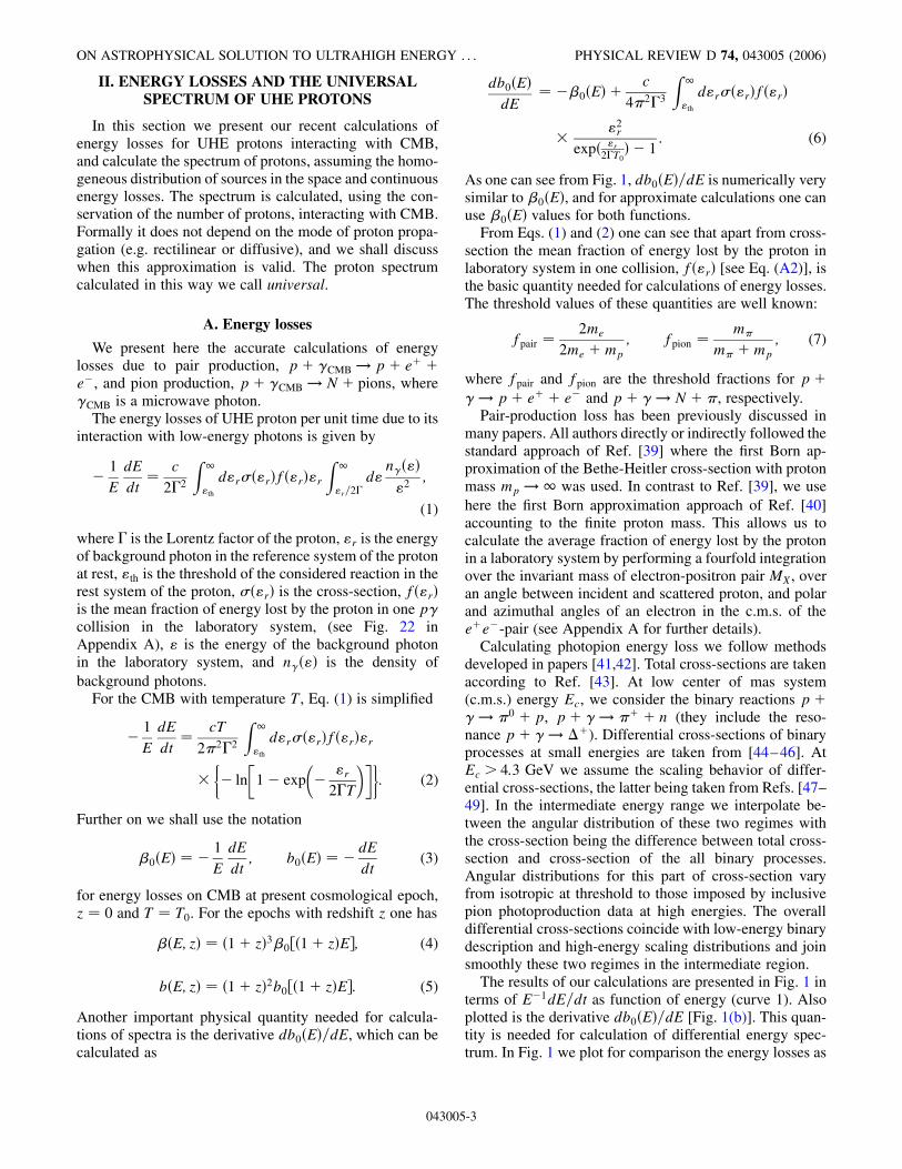
The results of our calculations are presented in Fig. 1 interms of E�1dE=dt as function of energy (curve 1). Alsoplotted is the derivative db0�E�=dE [Fig. 1(b)]. This quan-tity is needed for calculation of differential energy spec-trum. In Fig. 1 we plot for comparison the energy losses as

ON ASTROPHYSICAL SOLUTION TO ULTRAHIGH ENERGY . . . PHYSICAL REVIEW D 74, 043005 (2006)

043005-3

calculated by Berezinsky and Grigorieva 1988 [50](dashed curve 2). The difference in energy losses due topion production is very small, not exceeding 5% in theenergy region relevant for comparison with experimentaldata (E 1021 eV). The difference with energy losses dueto pair production is larger and reaches maximal value15%. The results of calculations by Stanev et al. [51] areshown by black squares. These authors have performed thedetailed calculations for both aforementioned processes,though their approach is different from ours, especially forthe photopion process. Our new energy losses are practi-cally indistinguishable from Stanev et al. [51] for pairproduction and pion production at low energies, and differby 15%–20% for pion production at highest energies (seeFig. 1). Stanev et al. claimed that energy losses due to pairproduction is underestimated by Berezinsky andGrigorieva [50] by 30%– 40%. Comparison of data filesof Stanev et al. and Berezinsky and Grigorieva (see alsoFig. 1) shows that this difference is significantly less. Mostprobably, Stanev et al. scanned inaccurately the data fromthe journal version of the paper [50].

B. Universal spectrum

To calculate the spectrum one should first of all evolvethe proton energy E from the time of observation t � t0 (orz � 0) to the cosmological epoch of generation t (or red-shift z), using the adiabatic energy lossesEH�z� and b�E; z�given by Equation (4):

� dE=dt � EH�z� �1 z�2b0��1 z�E�; (8)

where H�z� � H0

��m�1 z�3 ��

pis the Hubble pa-

rameter at cosmological epoch z, with H0 �72 km=s Mpc, �m � 0:27 and �� 0:73 [52].

We calculate the spectrum from conservation of numberof particles in the comoving volume (protons change theirenergy but do not disappear). For the number of UHEprotons per unit comoving volume, np�E�, one has

np�E�dE �Z t0

tmin

dtQgen�Eg; t�dEg; (9)

where t is an age of the universe, Eg � Eg�E; t� is ageneration energy at age t, calculated according toEq. (8) and Qgen�Eg; t� is the generation rate per unitcomoving volume, which can be expressed through emis-sivity L0, the energy release per unit time and unit ofcomoving volume, at t � t0, as

Qgen�Eg; t� � L0�1 z�mKqgen�Eg�; (10)

where �1 z�m describes the possible cosmological evo-lution of the sources. In the case of the power-law genera-tion, qgen�Eg� � E

��gg , with normalization constant

K � �g � 2 for �g > 2 and K � �lnEmax=Emin��1 for

�g � 2. We remind the reader that in these formulas andeverywhere below, energies E are given in GeV, emissivityL in GeV cm�3 s�1, and source luminosity L in GeV s�1.

1017 1018 1019 1020 1021 102210-12

10-11

10-10

10-9

10-8

10-7

2

1e+e-

e+e- pion-prod.

red-shift

(a)

1/E

dE

/dt,

yr-1

E, eV

1017 1018 1019 1020 1021 102210-12

10-11

10-10

10-9

10-8

10-7

(b)

pion-prod.

red-shift

e+e-

db0(

E)/

dE, y

r-1; β

0(E

), y

r-1

E, eV

FIG. 1 (color online). (a) UHE proton energy losses E�1dE=dt at z � 0 (present work: curve 1; Berezinsky and Grigorieva (1988)[50]: curve 2; Stanev et al. 2000 [51]: black squares). The line ‘‘redshift’’ (H0 � 72 km=s Mpc) gives adiabatic energy losses. Notetwo important energies Eeq1 � 2:37� 1018 eV, where adiabatic and pair- production energy losses become equal, and Eeq2 �

6:05� 1019 eV, where pair-production and photopion production energy losses are equal. The latter is one of the characteristics of theGZK cutoff. (b) The derivative db0�E�=dE, where b0�E� � �dE=dt at present epoch z � 0, (solid curve) in comparison with �0�E� ��E�1dE=dt (dashed curve).


043005-4

From Eq. (9) one obtains the diffuse flux as

Jp�E� �c

4�L0K

Z zmax

0dz��dtdz

��1 z�mqgen�Eg�dEgdE

;

(11)

where jdt=dzj � H�1�z�=�1 z� and analytic expressionfor dEg=dE is given by Eq. (B6) in Appendix B.

The spectrum (11) is referred to as universal spectrum.Formally it is derived from conservation of the number ofparticles and does not depend on propagation mode [seeEq. (9)]. But in fact, the homogeneity of the particles,tacitly assumed in this derivation, implies the homogeneityof the sources, and thus the condition of validity of univer-sal spectrum is a small separation of sources. The homo-geneous distribution of particles in the case ofhomogeneous distribution of sources and inhomogeneousmagnetic fields follows from the Liouville theorem (seeRef. [53]).

Several effects could in principle modify the shape of theuniversal spectrum. They include propagation in magneticfields, discreteness in distribution of the sources, large-scale inhomogeneous distribution of sources, local sourceoverdensity or deficit, and fluctuations in interaction.These effects will be studied in the next sections. Withthe exception of energies beyond GZK cutoff and energiesbelow 1� 1018 eV, the universal spectrum is only weaklymodified by the aforementioned effects. Here we shortlycomment on the role of magnetic fields. As numericalsimulations (see e.g. [54,55]) show, the propagation ofUHE protons in strong magnetic fields changes the energyspectrum (for a physical explanation of this effect see[53]). The influence of a magnetic field on the spectrumdepends on the separation of the sources, d. For uniformdistribution of sources with separation d much less thancharacteristic lengths of propagation, such as attenuationlength latt and the diffusion length ldiff , the diffuse spec-trum of UHECR is the universal one independent of modeof propagation [53]. This statement has a status of thetheorem. For the wide range of magnetic fields 0.1–10 nG and distances between sources d & 50 Mpc, thespectrum at E> 1018 eV is close to the universal one [56].

C. Modification factor

The analysis of spectra is very convenient to perform interms of the modification factor. Modification factor isdefined as a ratio of the spectrum Jp�E� [see Eq. (11)]with all energy losses taken into account, to the unmodifiedspectrum Junm

p �E�, where only adiabatic energy losses(redshift) are included.

��E� �Jp�E�

Junmp �E�

: (12)

For the power-law generation spectrum for �g > 2 withoutevolution one has

Junmp �E��

c4��g�2�L0E

��gZ zmax

0dz��dtdz

��1z��g1:

(13)

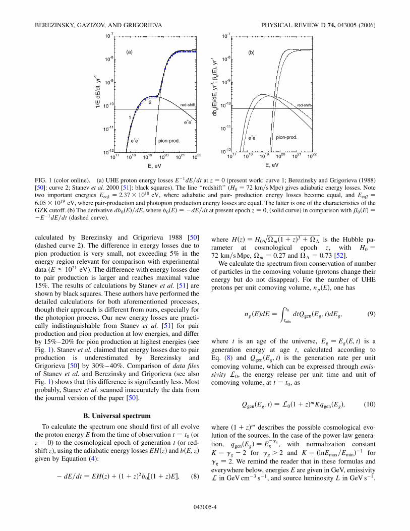
The modification factor is a less model-dependent quantitythan the spectrum. In particular, it should depend weaklyon �g, because both numerator and denominator inEq. (12) include E��g . In the next section we considerthe nonevolutionary case m � 0 (see Sec. IV E for discus-sion of evolution). In Fig. 2 the modification factor isshown as a function of energy for two spectrum indices�g � 2:0 and �g � 2:7. As expected above, they do notdiffer much from each other. Note that by definition��E� 1.

III. SIGNATURES OF UHE PROTONSINTERACTING WITH CMB

The extragalactic protons propagating through CMBhave signatures in the form of three spectrum features:GZK cutoff, dip, and bump. The dip is produced due toee�-production and bump—by pileup protons accumu-lated near the beginning of the GZK cutoff. We add herethe fourth signature: the second dip.

The analysis of these features, especially dip and bump,is convenient to perform in terms of the modification factor[50,57]. For the GZK cutoff we shall use the traditionalspectra.

1017 1018 1019 1020 1021

10-2

10-1

100

ηtotal

2

1 η

ee

2

1

1: γg=2.7

2: γg=2.0

mod

ifica

tion

fact

or

E, eV

FIG. 2 (color online). Modification factor for the power-lawgeneration spectra with �g in the range 2.0–2.7. Curve � � 1corresponds to adiabatic energy losses, curves �ee—to adiabaticand pair production energy losses and curves �tot —to all energylosses. The dip, seen at 1� 1018 E 4� 1019 eV, has twoflattenings: at low energy E � 1� 1018 eV and at high energyE � 1� 1019 eV. The second flattening explains well the ob-served spectrum feature, known as the ankle.


043005-5

A. GZK cutoff

The GZK cutoff [8,9] is most remarkable phenomenon,which describes the sharp steepening of the spectrum dueto pion production. The GZK cutoff is a model-dependentfeature of the spectrum, e.g. the GZK cutoff for a single

source depends on the distance to the source. A commonconvention is that the GZK cutoff is defined for diffuse fluxfrom the sources uniformly distributed over the universe.In this case one can give two definitions of the GZK cutoffposition. In the first one it is determined as the energy,EGZK � 4� 1019 eV, where the steep increase in the en-ergy losses starts (see Fig. 1). The GZK cutoff starts at thisenergy. The corresponding path length of a proton isRGZK � �E

�1dE=cdt��1 � 1:3� 103 Mpc. The advan-tage of this definition of the cutoff energy is the indepen-dence of a spectrum index, but this energy is too low tojudge about presence or absence of the cutoff in the mea-sured spectrum. A more practical definition is E1=2, wherethe flux with cutoff becomes lower by a factor of 2 thanpower-law extrapolation. This definition is convenient touse for the integral spectrum, which is better approximatedby the power-law function than the differential one. InFig. 3 the function E��1�J�>E�, where J�>E�, the calcu-lated integral diffuse spectrum, is plotted as a function ofenergy. Note that � > �g is an effective index of thepower-law approximation of the spectrum modified byenergy losses. For a wide range of generation indices 2:1 �g 2:7, the cutoff energy is the same, E1=2 �

5:3� 1019 eV. The corresponding proton path length isR1=2 � 800 Mpc. In panel (a) of Fig. 4 E1=2 is found fromthe integral spectrum of the Yakutsk array in the reasonableagreement with theoretical prediction. The HiRes data areshown in panel (b). These data have large uncertainties,which prevent the accurate determination of E1=2.However, they agree with the predicted value E1=2 � 5:3�1019 eV. In the recent paper [58] the Hires collaboration

18 19 20 21-2.0

-1.5

-1.0

-0.5

0.0

0.5

1.0

solid line: γg=2.1dashed line: γg=2.7

E1/2=5.3 1019

eV

log 10

E(γ

-1) J(

>E

)

log10

E,eV

FIG. 3. E1=2 as characteristic of the GZK cutoff. The calcu-lated integral spectra are multiplied to factor E��1, where �� 1found to fit the spectra in the interval 1� 1018–3� 1019 eV.E1=2 is shown by the vertical line. This value is valid forgeneration spectra with 2:1 �g 2:7.

1018 1019 1020 1021

1023

1024

1025

E1/2=5.3 1019eV

Yakutskγ

g=2.7

J(>

E)E

2 , eV

2 m-2s-1

sr-1

E, eV1018 1019 1020 1021

1023

1024

1025

E1/2=5.3 1019 eV

HiRes I - HiRes IIγ

g=2.7

J(>

E)E

2 ,eV

2 m-2s-1

sr-1

E, eV

FIG. 4 (color online). Predicted E1=2 value in comparison with integral spectrum of Yakutsk array (left panel) and HiRes (rightpanel). One can see the agreement of the Yakutsk data with the theoretical value E1=2 � 5:3� 1019 eV (vertical line), while in the caseof HiRes data this value is about 7� 1019 eV with large uncertainties due to difference between HiRes I and HiRes II data. HiRescollaboration found [58] E1=2 � �5:92:4

�0:8� � 1019 eV.


043005-6

foundE1=2 � �5:92:4�0:8� � 1019 eV in better agreement with

the predicted value.In Fig. 5 the calculated universal spectra with the GZK

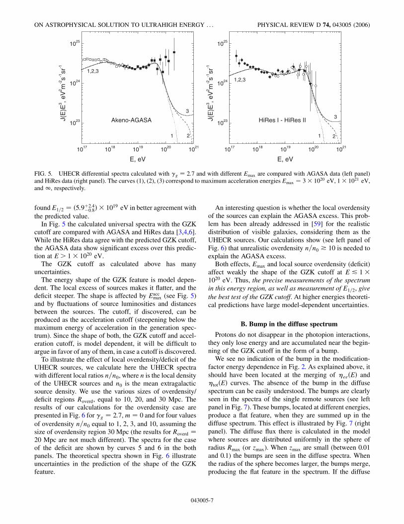
cutoff are compared with AGASA and HiRes data [3,4,6].While the HiRes data agree with the predicted GZK cutoff,the AGASA data show significant excess over this predic-tion at E> 1� 1020 eV.

The GZK cutoff as calculated above has manyuncertainties.

The energy shape of the GZK feature is model depen-dent. The local excess of sources makes it flatter, and thedeficit steeper. The shape is affected by Eacc

max (see Fig. 5)and by fluctuations of source luminosities and distancesbetween the sources. The cutoff, if discovered, can beproduced as the acceleration cutoff (steepening below themaximum energy of acceleration in the generation spec-trum). Since the shape of both, the GZK cutoff and accel-eration cutoff, is model dependent, it will be difficult toargue in favor of any of them, in case a cutoff is discovered.

To illustrate the effect of local overdensity/deficit of theUHECR sources, we calculate here the UHECR spectrawith different local ratios n=n0, where n is the local densityof the UHECR sources and n0 is the mean extragalacticsource density. We use the various sizes of overdensity/deficit regions Roverd, equal to 10, 20, and 30 Mpc. Theresults of our calculations for the overdensity case arepresented in Fig. 6 for �g � 2:7,m � 0 and for four valuesof overdensity n=n0 equal to 1, 2, 3, and 10, assuming thesize of overdensity region 30 Mpc (the results for Roverd �20 Mpc are not much different). The spectra for the caseof the deficit are shown by curves 5 and 6 in the bothpanels. The theoretical spectra shown in Fig. 6 illustrateuncertainties in the prediction of the shape of the GZKfeature.

An interesting question is whether the local overdensityof the sources can explain the AGASA excess. This prob-lem has been already addressed in [59] for the realisticdistribution of visible galaxies, considering them as theUHECR sources. Our calculations show (see left panel ofFig. 6) that unrealistic overdensity n=n0 * 10 is needed toexplain the AGASA excess.

Both effects, Emax and local source overdensity (deficit)affect weakly the shape of the GZK cutoff at E & 1�1020 eV. Thus, the precise measurements of the spectrumin this energy region, as well as measurement of E1=2, givethe best test of the GZK cutoff. At higher energies theoreti-cal predictions have large model-dependent uncertainties.

B. Bump in the diffuse spectrum

Protons do not disappear in the photopion interactions,they only lose energy and are accumulated near the begin-ning of the GZK cutoff in the form of a bump.

We see no indication of the bump in the modification-factor energy dependence in Fig. 2. As explained above, itshould have been located at the merging of �ee�E� and�tot�E� curves. The absence of the bump in the diffusespectrum can be easily understood. The bumps are clearlyseen in the spectra of the single remote sources (see leftpanel in Fig. 7). These bumps, located at different energies,produce a flat feature, when they are summed up in thediffuse spectrum. This effect is illustrated by Fig. 7 (rightpanel). The diffuse flux there is calculated in the modelwhere sources are distributed uniformly in the sphere ofradius Rmax (or zmax). When zmax are small (between 0.01and 0.1) the bumps are seen in the diffuse spectra. Whenthe radius of the sphere becomes larger, the bumps merge,producing the flat feature in the spectrum. If the diffuse

1017 1018 1019 1020 1021

1023

1024

1025

3

21

1,2,3

Akeno-AGASA J(E

)E3 , e

V2 m

-2s-1

sr-1

E, eV

1017 1018 1019 1020 1021

1023

1024

1025

3

21

1,2,3

HiRes I - HiRes IIJ(E

)E3 , e

V2 m

-2s-1

sr-1

E, eV

FIG. 5. UHECR differential spectra calculated with �g � 2:7 and with different Emax are compared with AGASA data (left panel)and HiRes data (right panel). The curves (1), (2), (3) correspond to maximum acceleration energies Emax � 3� 1020 eV, 1� 1021 eV,and 1, respectively.


043005-7

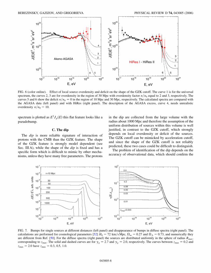
spectrum is plotted as E3Jp�E� this flat feature looks like apseudobump.

C. The dip

The dip is more reliable signature of interaction ofprotons with the CMB than the GZK feature. The shapeof the GZK feature is strongly model dependent (seeSec. III A), while the shape of the dip is fixed and has aspecific form which is difficult to mimic by other mecha-nisms, unless they have many free parameters. The protons

in the dip are collected from the large volume with theradius about 1000 Mpc and therefore the assumption of theuniform distribution of sources within this volume is welljustified, in contrast to the GZK cutoff, which stronglydepends on local overdensity or deficit of the sources.The GZK cutoff can be mimicked by acceleration cutoff,and since the shape of the GZK cutoff is not reliablypredicted, these two cases could be difficult to distinguish.

The problem of identification of the dip depends on theaccuracy of observational data, which should confirm the

1017 1018 1019 1020 102110-8

10-7

10-6

10-5

10-4

10-3

10-2

10-1

200

500

1000

100

5030

r=10 Mpc

J(E

) E

γ g , a

rb. u

nits

E, eV

1017 1018 1019 1020 102110-3

10-2

10-1

100

2.0

0.2

0.08

0.05

0.03

0.01

zmax=0.003

η(E

,zm

ax)

E, eV

FIG. 7. Bumps for single sources at different distances (left panel) and disappearance of bumps in diffuse spectra (right panel). Thecalculations are performed for cosmological parameters [52] H0 � 72 km=s Mpc, �m � 0:27 and �� 0:73, and numerically theyare different from Ref. [50]. For the diffuse spectra (right panel) the sources are distributed uniformly in the sphere of radius Rmax,corresponding to zmax. The solid and dashed curves are for �g � 2:7 and �g � 2:0, respectively. The curves between zmax � 0:2 andzmax � 2:0 have zmax � 0:3, 0.5, 1.0.

1017 1018 1019 1020 1021

1023

1024

1025

Akeno-AGASA

6 5

4

3

2

1

J(E

)E3 , m

-2s-1

sr-1eV

2

E, eV1017 1018 1019 1020 1021

1023

1024

1025

HiRes I - HiRes II

6 5

3

2

1

J(E

)E3 , m

-2s-1

sr-1eV

2

E, eV

FIG. 6 (color online). Effect of local source overdensity and deficit on the shape of the GZK cutoff. The curve 1 is for the universalspectrum, the curves 2, 3 are for overdensity in the region of 30 Mpc with overdensity factor n=n0 equal to 2 and 3, respectively. Thecurves 5 and 6 show the deficit n=n0 � 0 in the region of 10 Mpc and 30 Mpc, respectively. The calculated spectra are compared withthe AGASA data (left panel) and with HiRes (right panel). The description of the AGASA excess, curve 4, needs unrealisticoverdensity n=n0 � 10.


043005-8

specific (and well predicted) shape of this feature. Do thepresent data have the needed accuracy?

The comparison of the calculated modification factorwith that obtained from the Akeno-AGASA data, using�g � 2:7, is given in Fig. 8. It shows the excellent agree-ment between predicted and observed modification factorsfor the dip. In Fig. 8 one observes that at E< 1� 1018 eVthe agreement between calculated and observed modifica-tion factors becomes worse and the observational modifi-cation factor becomes larger than 1. Since by definition��E� 1, it evidences for appearance of another compo-nent of cosmic rays, which is almost undoubtedly given bygalactic cosmic rays. The condition �> 1 implies thedominance of the new (galactic) component, the transitionoccurs at E< 1� 1018 eV.

To calculate �2 for the confirmation of the dip byAkeno-AGASA data, we choose the energy interval be-tween 1� 1018 eV and 4� 1019 eV [the energy of theintersection of �ee�E� and �tot�E�]. In calculations, we

used the Gaussian statistics for low-energy bins and thePoisson statistics for the high energy bins of AGASA. Itresults in �2 � 19:06. The number of Akeno-AGASA binsis 19. We use in calculations two free parameters: �g andthe total normalization of spectrum. In effect, the confir-mation of the dip is characterized by �2 � 19:06 ford:o:f: � 17, or �2=d:o:f: � 1:12, very close to the idealvalue 1.0 for the Poisson statistics.

In the right upper panel of Fig. 8 the comparison of themodification factor with the HiRes data is shown. Theagreement is also very good: �2 � 19:5 for d:o:f: � 19for the Poisson statistics. The Yakutsk and Fly’s Eye data(not shown here) agree with dip as well. The Auger spec-trum [7] at this preliminary stage does not contradict thedip.

The good agreement of the shape of the dip �ee�E� withobservations is a strong evidence for extragalactic protonsinteracting with the CMB. This evidence is confirmed bythe HiRes data on the mass composition [13,14]. While the

1017 1018 1019 1020 1021

10-2

10-1

100

Akeno-AGASA

ηtotal

ηee

γg=2.7

mod

ifica

tion

fact

or

E, eV

1017 1018 1019 1020 1021

10-2

10-1

100

ηtotal

HiRes I - HiRes II

ηee

γg=2.7

mod

ifica

tion

fact

or

E, eV

1017 1018 1019 1020 1021

10-2

10-1

100

Yakutsk

ηtotal

ηee

γg=2.7

mod

ifica

tion

fact

or

E, eV1017 1018 1019 1020 1021

10-2

10-1

100

γg=2.7

Auger

ηtotal

ηee

mod

ifica

tion

fact

or

E, eV

FIG. 8 (color online). Predicted dip in comparison with AGASA, HiRes, Yakutsk and Auger [7] data.


043005-9

data of the Yakutsk array [16] and HiRes-MIA [15] supportthis mass composition, and Haverah Park data [1] do notcontradict it at E * �1–2� � 1018 eV, the data of Akeno[17] and Fly’s Eye [5] favor the mixed composition domi-nated by heavy nuclei.

The observation of the dip should be considered asindependent evidence in favor of proton-dominated pri-mary composition in the energy range 1� 1018–4�1019 eV.

D. The second dip

The second dip in the spectrum of extragalactic UHEprotons appears at energy E � 6:3� 1019 due to interplaybetween pair production and photopion production. It is thedirect consequence of energy Eeq2 � 6:05� 1019 eV,where energy losses due to ee�-production and pion-production become equal (see Fig. 1). This spectrum fea-ture is explained as follows.

The pion-production energy loss increases with energyvery fast, and at energy slightly below Eeq2

ee�-production dominates and spectrum can be withhigh accuracy described in continuous energy-loss ap-proximation. At energy slightly higher than Eeq2 thepion-production dominates and the precise calculation ofspectrum should be performed in the kinetic-equation ap-proach. In this method the evolution of number of particlesin interval dE is given by two compensating terms, describ-ing the particle exit and regeneration due to p� collisions.The small continuous energy losses affect only the exitterm and break this compensation, diminishing the flux.The exact calculations are given in Appendix D. Thesecond dip is very narrow and its amplitude at maximumreaches �10% (see Fig. 24). This feature can be observedby detectors with very good energy resolution, and it givesthe precise mark for energy calibration of a detector. It canbe observed only marginally by the Auger detector.

IV. ROBUSTNESS OF THE DIP PREDICTION

We calculated the dip for the universal spectrum, i.e. forthe case when distances between sources are small enough,and the spectrum does not depend on the propagationmode. In this section we shall study stability of the diprelative to other possible phenomena, namely, discretenessin the source distribution, propagation in magnetic fields,etc. We shall consider also some phenomena related to theexistence of the dip.

A. Discreteness in the source distribution

As it follows from analysis of the small-scale anisotropy(see [22–26]), the average distance between UHECRsources is d� 30–50 Mpc [27,28]. Such discreteness af-fects the spectrum, especially at highest energies, whenenergy attenuation length is comparable with d. In thissubsection we demonstrate the stability of the dip relative

to discreteness of the sources. We illustrate the effect ofdiscreteness by an example of UHE protons propagatingrectilinearly from sources located in the vertices of a 3Dcubic lattice with spacing d. Positions of sources are givenby coordinates x � id, y � jd, and z � kd, where i, j, k �0;�1;�2 . . . . The observer is assumed at x � y � z � 0with no source there. The diffuse flux for the power-lawgeneration spectrum / E

��gg is given by summation over

all vertices. The maximum distance is defined by themaximum redshift zmax. Then the observed flux is given by

Jp�E� ��g � 2�L0d

�4��2Xi;j;k

Eg�E; zijk��g

�i2 j2 k2��1 zijk�

dEgdE

;

(14)

where L0 � Lp=d3 is emissivity, zijk is the redshift for a

source with coordinates i, j, k, and factor �1 zijk� takesinto account the time dilation.

The calculated spectra for d � 1, 5, 10, 20, 40, and60 Mpc are shown in Fig. 9 in comparison with theAGASA-Akeno data. In calculations we used Emax � 1�1022 eV, m � 0 (no evolution), zmax � 4 and �g � 2:7.Emissivity L0 is chosen to fit the AGASA data. One cansee that discreteness in the source distribution affectsweakly the dip, but the effect is more noticeable for theshape of the GZK cutoff.

With d decreasing, the calculated spectra regularly con-verge to the universal one, as it should be according topropagation theorem [53]. This theorem ensures also thatthe spectra from Fig. 14 are valid for the case of weakmagnetic field when the diffusion length ldiff * d.

B. Dip in the case of diffusive propagation

The dip, seen in the universal spectrum, is also present inthe case of diffusive propagation in magnetic fields [56].The calculations are performed for diffusion in random

FIG. 9. Proton spectra for rectilinear propagation from discretesources. Sources are located in vertices of 3D cubic grid withspacing d � 60, 40, 20, 10, 5, and 1 Mpc. The calculations areperformed for zmax � 4, Emax � 1� 1022 eV and �g � 2:7.


043005-10

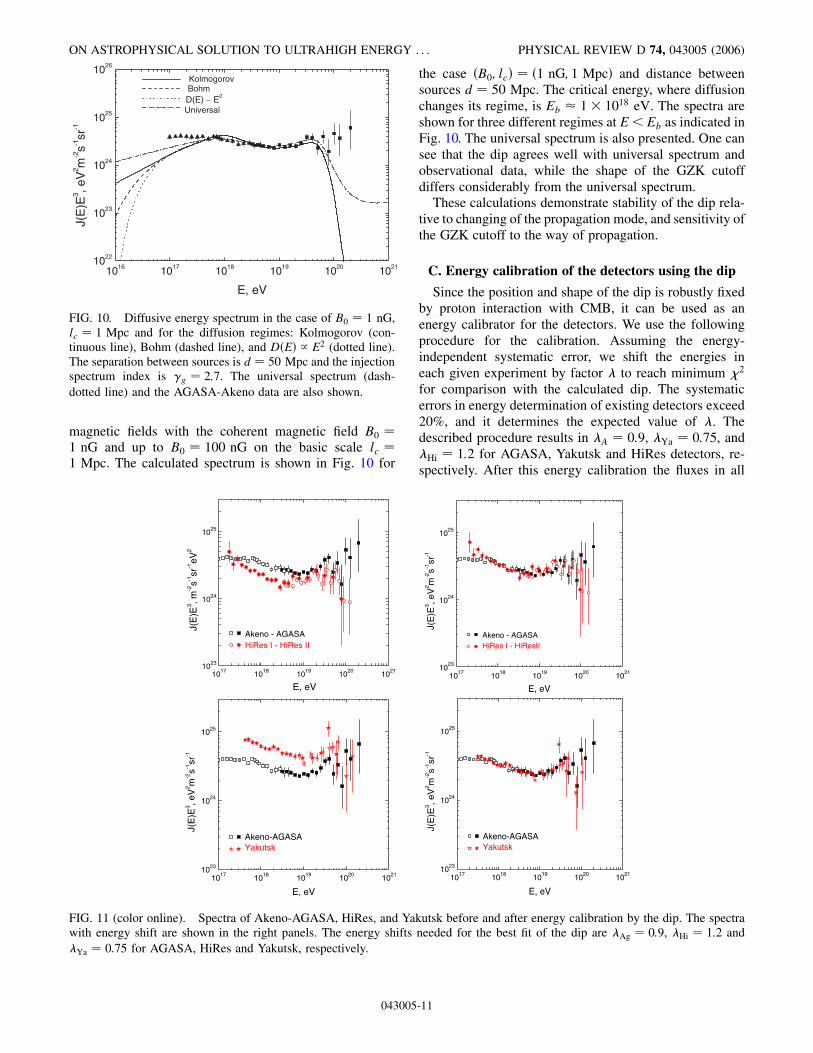
magnetic fields with the coherent magnetic field B0 �1 nG and up to B0 � 100 nG on the basic scale lc �1 Mpc. The calculated spectrum is shown in Fig. 10 for

the case �B0; lc� � �1 nG; 1 Mpc� and distance betweensources d � 50 Mpc. The critical energy, where diffusionchanges its regime, is Eb � 1� 1018 eV. The spectra areshown for three different regimes at E< Eb as indicated inFig. 10. The universal spectrum is also presented. One cansee that the dip agrees well with universal spectrum andobservational data, while the shape of the GZK cutoffdiffers considerably from the universal spectrum.

These calculations demonstrate stability of the dip rela-tive to changing of the propagation mode, and sensitivity ofthe GZK cutoff to the way of propagation.

C. Energy calibration of the detectors using the dip

Since the position and shape of the dip is robustly fixedby proton interaction with CMB, it can be used as anenergy calibrator for the detectors. We use the followingprocedure for the calibration. Assuming the energy-independent systematic error, we shift the energies ineach given experiment by factor � to reach minimum �2

for comparison with the calculated dip. The systematicerrors in energy determination of existing detectors exceed20%, and it determines the expected value of �. Thedescribed procedure results in �A � 0:9, �Ya � 0:75, and�Hi � 1:2 for AGASA, Yakutsk and HiRes detectors, re-spectively. After this energy calibration the fluxes in all

1017 1018 1019 1020 10211023

1024

1025

Akeno - AGASAHiRes I - HiRes II

J(E

)E3 , m

-2s-1

sr-1eV

2

E, eV1017 1018 1019 1020 1021

1023

1024

1025

Akeno - AGASAHiRes I - HiResII

J(E

)E3 , e

V2 m

-2s-1

sr-1

E, eV

1017 1018 1019 1020 10211023

1024

1025

Akeno-AGASAYakutsk

J(E

)E3 , e

V2 m

-2s-1

sr-1

E, eV

1017 1018 1019 1020 10211023

1024

1025

Akeno-AGASAYakutsk

J(E

)E3 , e

V2 m

-2s-1

sr-1

E, eV

FIG. 11 (color online). Spectra of Akeno-AGASA, HiRes, and Yakutsk before and after energy calibration by the dip. The spectrawith energy shift are shown in the right panels. The energy shifts needed for the best fit of the dip are �Ag � 0:9, �Hi � 1:2 and�Ya � 0:75 for AGASA, HiRes and Yakutsk, respectively.

1016 1017 1018 1019 1020 10211022

1023

1024

1025

1026

D(E) ∼ E2

Universal

BohmKolmogorov

J(E

)E3 , e

V2 m

-2s-1

sr-1

E, eV

FIG. 10. Diffusive energy spectrum in the case of B0 � 1 nG,lc � 1 Mpc and for the diffusion regimes: Kolmogorov (con-tinuous line), Bohm (dashed line), and D�E� / E2 (dotted line).The separation between sources is d � 50 Mpc and the injectionspectrum index is �g � 2:7. The universal spectrum (dash-dotted line) and the AGASA-Akeno data are also shown.


043005-11

experiments agree with each other. First, we consider theAGASA and HiRes data. There are two discrepanciesbetween these data (see the upper left panel of Fig. 11):one is described by factor 1.5–2.0 in energy region 1�1018–8� 1019 eV, and the second at E � 1� 1020 eV. InFig. 11, the spectra of Akeno-AGASA and HiRes areshown before and after the energy calibration. One cansee the good agreement of the calibrated data at E< 1�1020 eV and their consistency at E> 1� 1020 eV. Thisresult should be considered together with calculations [60],where it was demonstrated that 11 superGZK AGASAevents can be simulated by the spectrum with GZK cutoffin the case of 30% error in energy determination. We maytentatively conclude that existing discrepancies betweenAGASA and HiRes spectra at all energies are due tosystematic energy errors and statistics.

In Fig. 11, the energy spectra are shown for AGASA andYakutsk spectra before and after energy calibration. Again,the best fit to the dip shape results in excellent agreement inthe absolute values of fluxes.

The agreement between spectra of all three detectorsafter energy calibration by the dip confirms the dip as thespectrum feature produced by interaction of the protonswith the CMB, and demonstrates compatibility of fluxesmeasured by AGASA, HiRes, and Yakutsk detectors.

D. Dip and extragalactic UHE nuclei

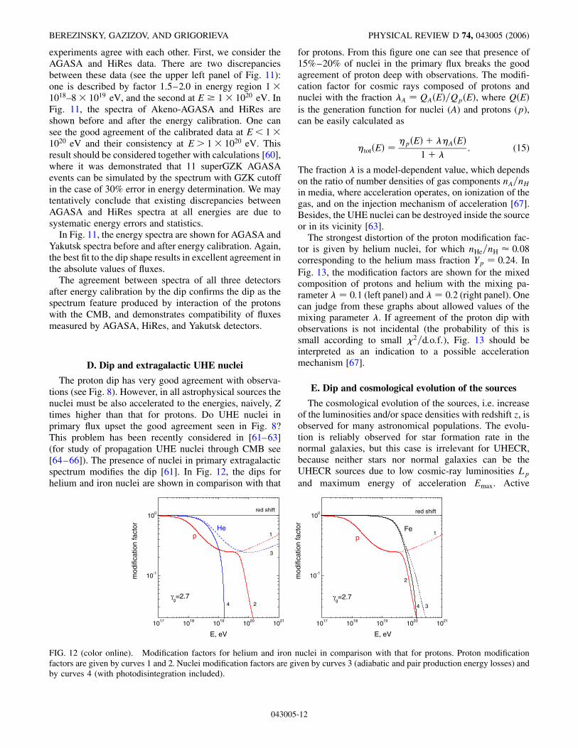
The proton dip has very good agreement with observa-tions (see Fig. 8). However, in all astrophysical sources thenuclei must be also accelerated to the energies, naively, Ztimes higher than that for protons. Do UHE nuclei inprimary flux upset the good agreement seen in Fig. 8?This problem has been recently considered in [61–63](for study of propagation UHE nuclei through CMB see[64–66]). The presence of nuclei in primary extragalacticspectrum modifies the dip [61]. In Fig. 12, the dips forhelium and iron nuclei are shown in comparison with that

for protons. From this figure one can see that presence of15%–20% of nuclei in the primary flux breaks the goodagreement of proton deep with observations. The modifi-cation factor for cosmic rays composed of protons andnuclei with the fraction �A � QA�E�=Qp�E�, where Q�E�is the generation function for nuclei (A) and protons (p),can be easily calculated as

�tot�E� ��p�E� ��A�E�

1 �: (15)

The fraction � is a model-dependent value, which dependson the ratio of number densities of gas components nA=nHin media, where acceleration operates, on ionization of thegas, and on the injection mechanism of acceleration [67].Besides, the UHE nuclei can be destroyed inside the sourceor in its vicinity [63].

The strongest distortion of the proton modification fac-tor is given by helium nuclei, for which nHe=nH � 0:08corresponding to the helium mass fraction Yp � 0:24. InFig. 13, the modification factors are shown for the mixedcomposition of protons and helium with the mixing pa-rameter � � 0:1 (left panel) and � � 0:2 (right panel). Onecan judge from these graphs about allowed values of themixing parameter �. If agreement of the proton dip withobservations is not incidental (the probability of this issmall according to small �2=d:o:f:), Fig. 13 should beinterpreted as an indication to a possible accelerationmechanism [67].

E. Dip and cosmological evolution of the sources

The cosmological evolution of the sources, i.e. increaseof the luminosities and/or space densities with redshift z, isobserved for many astronomical populations. The evolu-tion is reliably observed for star formation rate in thenormal galaxies, but this case is irrelevant for UHECR,because neither stars nor normal galaxies can be theUHECR sources due to low cosmic-ray luminosities Lpand maximum energy of acceleration Emax. Active

1017 1018 1019 1020 1021

10-1

100red shift

He

4

3

2

1p

γg=2.7

mod

ifica

tion

fact

or

E, eV

1017 1018 1019 1020 1021

10-1

100 red shift

4 3

2

1Fe

p

γg=2.7

mod

ifica

tion

fact

or

E, eV

FIG. 12 (color online). Modification factors for helium and iron nuclei in comparison with that for protons. Proton modificationfactors are given by curves 1 and 2. Nuclei modification factors are given by curves 3 (adiabatic and pair production energy losses) andby curves 4 (with photodisintegration included).


043005-12

Galactic Nuclei (AGN), which satisfy these requirements,also exhibit the evolution seen in radio, optical, and x-rayobservations. The x-ray radiation is probably the mostrelevant tracer for evolution of UHECR because bothradiations are feed by the energy release provided byaccretion to massive black hole: x rays—through radiationof accretion disk, and UHECR—through acceleration inthe jets. According to recent detailed analysis in [68,69] theevolution of AGN seen in x-ray radiation can be describedby factor �1 z�m up to zc � 1:2 and is saturated at largerz. In [68] the pure luminosity evolution and pure densityevolution are allowed with m � 2:7 and m � 4:2, respec-tively, and with zc � 1:2 for both cases. In [69] the pure

luminosity evolution is considered as preferable with m �3:2 and zc � 1:2. These authors do not distinguish betweendifferent morphological types of AGN. It is possible thatsome AGN undergo weak cosmological evolution, or noevolution at all. The important as potential UHECRsources, BL Lacs [30], show no signs of positive cosmo-logical evolution [70].

In the case of UHECR there is no need to distinguishbetween luminosity and density evolution, because thediffuse flux is determined by the emissivity, which includesboth luminosity and space evolution, as it follows fromEq. (10).

In Fig. 14 we present the calculated dip spectrum inevolutionary models, inspired by the data cited above. Forcomparison we show also the case of the absence ofevolution m � 0, as can be valid for BL Lacs. FromFig. 14 one can see that the spectra with evolution up tozc > 1 can explain the observational data down to a few�1017 eV and even below, in accordance with early calcu-lations [71–73] (see [74] for recent analysis). However, forany reasonable magnetic fields, protons with these energieshave small diffusion lengths and the spectrum acquires thediffusion ‘‘cutoff’’ at energy Eb � 1� 1018 eV (seeSec. IV B).

We conclude that for many reasonable evolution regimesthe dip agrees with observational data as well as the non-evolutionary case m � 0.

V. ROLE OF INTERACTION FLUCTUATIONS

UHE proton spectrum is affected by fluctuations in thephotopion production. These fluctuations may change theproton spectrum only at energy substantially higher thanE � 4� 1019 eV. At this energy the half of energy lossesis caused by ee� production which does not fluctuate. Upto energy 1� 1020 eV, the photoproduction of pions oc-curs at the threshold in collisions with photons from thehigh-energy tail of the Planck distribution, and the fractionof energy lost does not fluctuate, being fixed by the thresh-

1017 1018 1019 1020 10211023

1024

1025

3

1,2

1 - γg=2.6, m=2.4, z

c=1.2

2 - γg=2.65, m=1.8, z

c=1.2

3 - γg=2.7, m=0

J(E

)E3 , m

-2s-1

sr-1eV

2

E, eV

FIG. 14 (color online). The dip in evolutionary models incomparison with the AGASA data. The parameters of evolutionused in the calculations for curves 1 and 2 are similar to thoseobserved for AGN. The curve 3 is for m � 0.

1017 1018 1019 1020 102110-2

10-1

100red shift

γg=2.7

mod

ifica

tion

fact

or

E, eV

1017 1018 1019 1020 102110-2

10-1

100red shift

γg=2.7

mod

ifica

tion

fact

or

E, eV

FIG. 13 (color online). Modification factors for the mixed composition of protons and helium nuclei in comparison with AGASAdata. The left panel corresponds to mixing parameter � � 0:1, and the right panel to � � 0:2.


043005-13

old value. Indeed, for Ep � 1� 1020 eV the minimal en-ergy of CMB photons needed for pion production is � �3� 10�3 eV to be compared with the energy of photons inthe Planck distribution maximum �m � 3:7� 10�4 eV.The only fluctuating value is the interaction length.

The noticeable effect of fluctuations is expected forprotons with energies E> 1� 1020 eV.

As it is well known [75,76], the kinetic equations give anadequate method to account for the fluctuations in interac-tion. Neglecting the conversion of proton to neutron (neu-tron decays back to proton with small energy loss), thekinetic equation for UHE protons with adiabatic energylosses and with p �! p e e� and p �! N pions scattering in collisions with CMB photons can bewritten down as follows:

@np�E; t�

@t� �3H�t�np�E; t�

@@Ef�H�t�E

bpair�E; t��np�E; t�g � P�E; t�np�E; t�

Z Emax

EdE0P�E0; E; t�np�E

0; t� Qgen�E; t�;

(16)

where np�E; t� is the number density of UHE protons perunit energy, Qgen�E; t� is the generation rate, given byEq. (10) with m � 0, and H�t� is the Hubble parameter.The first term in the right-hand side of Eq. (16) describesexpansion of the universe. The energy loss bpair�E� due toee�-pair production is treated as continuous energy loss.The photopion collisions are described with the help of theprobability P�E; t� of proton exit from energy interval�E;E dE� due to p�-collisions and with the help of theirregeneration in the same energy interval described by theprobability P�E0; E; t�. These two probabilities describefluctuations in the interaction length and in the fractionof energy lost in the interaction; the interaction length isequivalent in this picture to the time of proton exit fromenergy interval dE. The exit probability P�E; t� due tocollisions with CMB photons with temperature T can bewritten as

P�E; t� � �cT

4�2E2

Z 1m�mp

dEcEc�E2c �m2

p��Ec�

� ln�

1� exp��E2c �m2

p

4ET

��; (17)

where Ec is the total c.m.s. energy of colliding proton andphoton, Emin

c � m� mp, ��Ec� is the photopion cross-section, and T is the CMB temperature at cosmologicalepoch t.

Similarly, in the regeneration term of Eq. (16) the proba-bility for a proton with energy E0 to produce a proton withenergy E is given by

P�E0; E; t� � �cT

4�2�E0�2Z 1Eminc �x�

dEcEc�E2c �m2

p�

�d��Ec; E

0; E�dE

ln�

1� exp��E2c �m

2p

4E0T

��;

(18)

where E0 and E are the energies of primary and secondaryprotons, respectively, and x � E=E0. The minimum valueof the allowed c.m.s. energy in this case is given by

Eminc �x� � �m2

�=�1� x� m2p=x�1=2: (19)

This bound corresponds to the process with minimuminvariant mass, namely, to p �! �0 p.

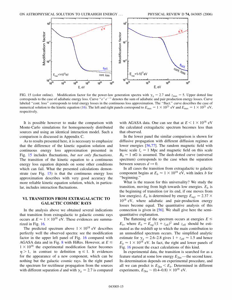
We have solved Eq. (16) numerically. The calculatedspectrum Jp�E� � �c=4��np�E; t0�, where t0 is the age ofthe universe at redshift z � 0, is presented in Fig. 15 as themodification factor ��E� � Jp�E�=J

unmp �E� for generation

spectrum with �g � 2:7 and Emax � 1� 1023 eV (leftpanel) andEmax � 1� 1021 eV (right panel). For compari-son the modification factors for a universal spectrum withcontinuous energy losses are also shown. The difference inthese two spectra at highest energies must be due tofluctuations in energy losses, though formally we have tosay that this is the difference between the solution tokinetic equation (16) and the continuous energy loss ap-proximation. For Emax � 1� 1023 eV one can see thedifference in the spectra about 25% at highest energiesand a tiny difference above the intersection of the �ee and�tot curves. For Emax � 1� 1021 eV the difference issmall.

Note that modification factors do not vanish at Emax,even when generation function goes abruptly to zero, sinceboth solutions vanish keeping the same value of ratios��E� � Jp�E�=Junm�E�. It is easy to demonstrate analyti-cally that the ratio of flux in continuous loss approximationJcont�E� to unmodified flux Junm�E�, given by Eq. (13),tends to H0=�coll�Emax� � 2:45� 10�3, when E! Emax.From Fig. 15 one can see that this ratio coincides exactlywith our numerical calculations, and this gives a proof thatour numerical calculations are correct.

The effect of interaction fluctuations is usually takeninto account with the help of Monte-Carlo simulations. Themethod of the kinetic equation corresponds to averagingover a large number of Monte-Carlo simulations, and if allother assumptions are the same, the results must coincideexactly. These assumptions include Emax and parameters ofp�-interaction. However, the existing Monte-Carlo simu-lations in most cases include some other assumptions incomparison with kinetic equations, which modify the spec-trum stronger than interaction fluctuations. One of them isdiscreteness in the source distribution (in kinetic equationsthe homogeneous distribution is assumed), the other isfluctuations of distances to the nearby sources.


043005-14

It is possible however to make the comparison withMonte-Carlo simulations for homogeneously distributedsources and using an identical interaction model. Such acomparison is discussed in Appendix C.

As to results presented here, it is necessary to emphasizethat the difference of the kinetic equation solution andcontinuous energy loss approximation presented inFig. 15 includes fluctuations, but not only fluctuations.The transition of the kinetic equation to a continuousenergy loss equation depends on some other conditionswhich can fail. What the presented calculations demon-strate (see Fig. 15) is that the continuous energy lossapproximation describes with very good accuracy themore reliable kinetic equation solution, which, in particu-lar, includes interaction fluctuations.

VI. TRANSITION FROM EXTRAGALACTIC TOGALACTIC COSMIC RAYS

In the analysis above we obtained several indicationsthat transition from extragalactic to galactic cosmic raysoccurs at E � 1� 1018 eV. These evidences are summa-rized in Fig. 16.

The predicted spectrum above 1� 1018 eV describesperfectly well the observed spectra: see the modificationfactor in the upper left panel of Fig. 16 compared withAGASA data and in Fig. 8 with HiRes. However, at E &

1� 1018 the experimental modification factor becomes�> 1, in contrast to definition � 1. It evidencesfor the appearance of a new component, which can benothing but the galactic cosmic rays. In the right panelthe spectrum for rectilinear propagation from the sourceswith different separation d and with �g � 2:7 is compared

with AGASA data. One can see that at E< 1� 1018 eVthe calculated extragalactic spectrum becomes less thanthat observed.

In the lower panel the similar comparison is shown fordiffusive propagation with different diffusion regimes atlower energies [56,77]. The random magnetic field withbasic scale lc � 1 Mpc and magnetic field on this scaleB0 � 1 nG is assumed. The dash-dotted curve (universalspectrum) corresponds to the case when the separationbetween sources d! 0.

In all cases the transition from extragalactic to galacticcomponent begins at Eb � 1� 1018 eV, with index b for‘‘beginning.’’

What is the reason for this universality? We study thetransition, moving from high towards low energies. Eb isthe beginning of transition (or its end, if one moves fromlow energies). Eb is determined by energy Eeq1 � 2:37�1018 eV, where adiabatic and pair-production energylosses become equal. The quantitative analysis of thisconnection is given in [56]. We shall give here the semi-quantitative explanation.

The flattening of the spectrum occurs at energies E Eb, where Eb � Eeq=�1 zeff�

2 and zeff should be esti-mated as the redshift up to which the main contribution toan unmodified spectrum occurs. The simplified analyticestimate for �g � 2:6–2:8 gives 1 zeff � 1:5 and henceEb � 1� 1018 eV. In fact, the right and lower panels ofFig. 16 present the exact calculations of this kind.

In experimental data, the transition is searched for as afeature started at some low energy E2kn —the second knee.Its determination depends on experimental procedure, andall we can predict is E2kn <Eb. Determined in differentexperiments, E2kn � �0:4–0:8� � 1018 eV.

FIG. 15 (color online). Modification factor for the power-law generation spectra with �g � 2:7 and zmax � 5. Upper dotted linecorresponds to the case of adiabatic energy loss. Curve ‘‘ee�’’ denotes the sum of adiabatic and pair production energy losses. Curvelabeled ‘‘cont. loss’’ corresponds to total energy losses in the continuous loss approximation. The ‘‘fluct.’’ curve describes the case ofnumerical solution to the kinetic equation (16). The left and right panels correspond to Emax � 1� 1023 eV and Emax � 1� 1021 eV,respectively.


043005-15

The transition at the second knee appears also in thestudy of propagation of cosmic rays in the Galaxy (see e.g.[78–80]).

Being thought of as a purely galactic feature, the posi-tion of the second knee in our analysis appears as a directconsequence of extragalactic proton energy losses.

The transition at the second knee is illustrated by Fig. 17.The clue to understanding this transition is given by theKASCADE data [81,82]. They confirm the rigidity model,according to which position of a knee for nuclei withcharge Z is connected with the position of the protonknee Ep as EZ � ZEp. There are two versions of thismodel. One is the confinement-rigidity model (bendingabove the knee is due to insufficient confinement in thegalactic magnetic field), and the other is the acceleration-rigidity model (Emax is determined by rigidity). In bothmodels the heaviest nuclei (iron) start to disappear at E>EFe � 6:5� 1016 eV, if the proton knee is located at Ep �2:5� 1015 eV. The shape of the spectrum above the ironknee (E> EFe) is model dependent, with two reliablypredicted features: it must be steeper than the spectrumbelow the iron knee (E< EFe), shown by the dash-dotcurve, and iron nuclei must be the dominant componentthere (see Fig. 17). The high energy part of the spectrumhas a characteristic energy Eb, below which the spectrumbecomes more flat, i.e. drops down when multiplied to E2:5

(see Fig. 17). This part of the spectrum is shown for the

diffusive propagation described in Sec. VII B. These twofalling parts of the spectrum inevitably intersect at someenergy Etr, which can be defined as transition energy fromgalactic to extragalactic cosmic rays. The ‘‘end’’ of galac-tic cosmic rays EFe � 6:5� 1016 eV and the beginning offull dominance of the extragalactic component Eb � 1�1018 eV differ by an order of magnitude. Note, that power-law extrapolation of the total galactic spectrum, shown bydot-dash line, beyond the iron knee EFe has no physicalmeaning in the rigidity models and must not be discussed.

The second-knee transition gives an alternative possibil-ity in comparison with the ankle-transition hypothesisknown from the end of the 1970s. It is inspired by flat-tening of the spectrum at Ea � 1� 1019 eV seen in theAGASA and Yakutsk data (left panels in Fig. 8) andpossibly at �0:5–1� � 1019 eV in the Hires data (the rightpanel in Fig. 8). Being multiplied to factor E2:5, as inFig. 17, the ankle transition looks very similar to that atthe second knee. Note that in the latter case the ankle is justan instrinsic part of the dip.

The ankle transition has been recently discussed inRefs. [62,83–86].

In the ankle model it is assumed that the galactic cosmicray spectrum has a power-law shape / E�� from theproton knee Ep � 2:5� 1015 eV to about Ea � 1�1019 eV where it becomes steeper and crosses the moreflat extragalactic spectrum (see the right panel of Fig. 17).

1017 1018 1019 1020 1021

10-2

10-1

100

Akeno-AGASA

ηtotal

ηee

γg=2.7

mod

ifica

tion

fact

or

E, eV

1016 1017 1018 1019 1020 10211022

1023

1024

1025

1026

D(E) E2

Universal

BohmKolmogorov

J(E

)E3 , e

V2 m

-2s-1

sr-1

E, eV

FIG. 16 (color online). Appearance of transition energy Eb � 1� 1018 eV in the modification factor compared with AGASA data(left panel), in the spectrum for rectilinear propagation from the sources with separation d indicated in the figure (right panel) and inthe spectrum for diffusive propagation (lower panel).


043005-16

The ankle transition in Fig. 17 is shown for the extraga-lactic proton spectrum with generation index �g � 2,while the galactic spectrum, given by curve ‘‘gal.CR,’’ iscalculated as the difference of the observed total spectrumand calculated extragalactic proton spectrum.

The ankle model has problems with the galactic compo-nent of cosmic rays. The spectrum at 1� 1018–1�1019 eV is taken ad hoc to fit the observations, while inthe second-knee model this part of the spectrum is calcu-lated with excellent agreement with the data. In the rigiditymodels, the heaviest nuclei (iron) start to disappear at E>EFe � 6:5� 1016 eV. How is the gap between 1�1017 eV and 1� 1019 eV filled?

Galactic protons start to disappear at E> 2:5�1015 eV. Where did they come from at E> 1� 1017 eVto be seen e.g. in the Akeno detector with fraction 10%?

The ankle model needs acceleration by galactic sourcesup to 1� 1019 eV (at least for iron nuclei), which isdifficult to afford. The second-knee model amelioratesthis requirement by 1 order of magnitude.

The second-knee model predicts the spectrum shapedown to 1� 1018 eV with extremely good accuracy(�2=d:o:f: � 1:12 for Akeno-AGASA and �2=d:o:f: �1:03 for HiRes). In the ankle model one has to considerthis agreement as accidental, though such hypothesis hasvery low probability, determined by �2 cited above. As analternative, the ankle model-builders can suggest onlyhopes for future development of galactic propagation mod-els to be as precisely calculated as the dip.

VII. ASTROPHYSICAL SOURCES OF UHECR

In the sections above we have performed the model-independent analysis of spectra of extragalactic protonsinteracting with CMB. We have calculated the features ofthe proton spectrum assuming the power-law generationspectrum / E��g valid at E � 1� 1018 eV, and comparedpredicted features with observations. We found that protondip, a model-independent feature at energy between 1�1018 eV and 4� 1019 eV, is well confirmed by observa-tions. Only two free parameters are involved in fitting ofobservational data: �g � 2:7 (the allowed range is 2.55–2.75) and the flux normalization constant. The variousphysical phenomena included in calculations, such as dis-creteness in the source distribution, the different modes ofpropagation (rectilinear and diffusive), cosmological evo-lution with parameters similar to AGN evolution, fluctua-tions in p� interaction, etc., do not upset this agreement.

The transition of extragalactic to galactic cosmic rays isalso discussed basically in a model-independent manner.

In this section we shall discuss the models: realisticenergy spectra, the sources, and the models for transitionfrom extragalactic to galactic cosmic rays.

The UHECR sources have to satisfy two conditions:they must be very powerful and must accelerate particlesto large Emax * 1� 1021 eV. There is one more restriction[22–28], coming from observation of small-scale cluster-ing: the space density of the sources should be �1–3� �10�5 Mpc�3, probably with noticeable uncertainty in this

107 108 109 1010101

102

103

Eb

Et rE

Fe

extr. pgal. Fe

KASCADEHiRes IHiRes II

J(E

)E2.

5 , m-2s-1

sr-1G

eV1.

5

E, GeV

109 1010 1011100

101

102

Et r

gal. CR

HiRes IHiRes II

extr. p

J(E

)E2.

5 , m-2s-1

sr-1G

eV1.

5

E, GeV

FIG. 17 (color online). Transition from extragalactic to galactic cosmic rays in the second-knee (left panel) and ankle (right panel)models. In the left panel are shown: KASCADE total spectrum, which above the iron knee EFe is composed mostly by iron nuclei(‘‘gal.Fe’’ curve), below Eb the extragalactic proton spectrum (‘‘extr.p’’ curve) is calculated for diffusive propagation (see Sec. VII B)and Etr is the energy of the transition from galactic cosmic rays to extragalactic protons. The dot-dash line shows power-lawextrapolation of the low-energy KASCADE spectrum. In the right panel the extragalactic proton spectrum is calculated for generationspectrum / E�2, while the galactic spectrum (curve ‘‘gal.CR’’) is taken as difference between the observed total spectrum and thecalculated spectrum of extragalactic protons.


043005-17

value. Thus, these sources are more rare than typicalrepresentatives of AGN, e.g. Seyfert galaxies, whose spacedensity is �3� 10�4 Mpc�3. The sources could be therare types of AGN, and indeed the analysis of [30] showsstatistically significant correlation between directions ofparticles with energies �4–8� � 1019 eV and directions toAGN of the particular type—BL Lacs (see also criticism[31] and reply [32]). The acceleration in AGN can providethe maximum energy of acceleration up to �1021 eV fornonrelativistic shock acceleration (see e.g. [87]).

The relativistic shock acceleration can occur in AGNjets. Acceleration to Emax � 1021 eV in the AGN relativ-istic shocks is questionable (see discussion below).

Gamma ray bursts (GRBs) [88–90] are another poten-tially possible source of UHECR. They have very largeenergy output and can accelerate particles up to �1021 eV[89,90]. These sources have, however, the problems withexplaining small-angle anisotropy and with energetics (seediscussion below).

A. Spectra

The assumption of the power-law generation spectrumwith �g � 2:7 extrapolated to Emin � 1 GeV results in toolarge emissivity required for observed fluxes of UHECR.To avoid this problem the broken generation spectrum hasbeen suggested in Refs. [71,91]:

Qgen�E� ��/ E�2 at E Ec/ E�2:7 at E � Ec

; (20)

where Qgen�E� is the generation function (rate of particleproduction per unit of comoving volume), defined byEqs. (9) and (10), and Ec was considered as a freeparameter.

Recently it was demonstrated that the broken generationspectrum can naturally emerge under most reasonablephysical assumptions. In Ref. [92] it has been argued thatwhile spectrum E�2 is universal for nonrelativistic shockacceleration, the maximum acceleration energy Emax isnot, being dependent on the physical characteristics of asource, such as its size, regular magnetic field, etc.Distribution of sources over Emax results in steepening ofthe generation function, so that the distribution of thesources dn=dEmax / E

��max explains the observational

data, if � � 1:5–1:6 [92].In Appendix E we address the generalized problem:

what should be the distribution of spectral emissivityover Emax to provide the generation function with thebroken spectrum. We use there the notation " � Emax

and introduce the spectral emissivity L�"� � ns�"�Lp�"�,where Lp�"� is the particle luminosity of a source andns�"� � ns�"; Lp�"�� is the space density of the sources.The total emissivity is given by L0 �

RL�"�d".

Distribution of spectral emissivity L�"� over maximalenergies " determines the energy steepening of the gen-eration function Qgen�E� at energy E � "min in the distri-

bution. This function is calculated analytically for arbitraryL�"�, assuming that " is confined to the interval�"min; "max�. It is demonstrated that Qgen�E� can be thepower-law function / E��g exactly, only if the L�"� dis-tribution is power law, too ( / "��). For the source gen-eration function qgen�E� / E��2� at E ", thegeneration index in the interval "min E "max is foundto be �g � 1 �, including the case � 0. Thesteepening of the generation spectrum from 2 to �goccurs approximately at energy Ec � "min. At energy E>"max the spectrum is suppressed as exp��E="max� orstronger.

In the applications we are interested in two cases: � 0(nonrelativistic shocks) and � 0:2–0:3 (ultrarelativisticshocks). In the latter case the term E�2 in Eq. (20) shouldbe substituted by E��2�. The energy Ec � "min inEq. (20) is considered as a free parameter.

B. Active galactic nuclei

The AGN as sources of UHECR meet the necessaryrequirements: (i) to accelerate particles to Emax �1021 eV, (ii) to provide the necessary energy output, and(iii) to have the space density ns � �1–3� � 10�5 Mpc�3,required by small-scale clustering. We shall discuss belowthese problems in some detail.

1. Acceleration and spectra

The flow of the gas in AGN jet can be terminated by thenonrelativistic shock which accelerates protons or nuclei inthe radio lobe up to Emax � 1021 eV with spectrum / E�2

[87].In some cases the observed velocities in AGN jets are

ultrarelativistic with a Lorentz factor up to �� 5–10. It isnatural to assume there the existence of internal and exter-nal ultrarelativistic shocks. Acceleration in relativisticshocks relevant for UHECR has been recently studied inRefs. [89,90,93–98]. The acceleration spectrum is / E��gand in the case of isotropic scattering of particles upstreamand downstream, the spectrum index is �g � 2:23� 0:01[94]. However, recently it was understood that this resultdepends on scattering properties of the medium [96,98],and the spectrum can be steeper. In the regime of largeangle scattering in [96] �g � 2:7 was found to be possiblefor the shock with velocity u� �0:8–0:9�c with compres-sion ratio r � 2. In the Monte-Carlo simulation [98] it isdemonstrated that the effect of compression of upstreammagnetic field results in increasing of �g up to the limitingvalue 2.7 in ultrarelativistic case �sh � 1.

The maximal energy of acceleration Emax is a contro-versial issue. While in most works (very notably [93]) it isobtained that Emax cannot reach �1021 eV for all realisticcases of relativistic shocks, the authors of Ref. [99] argueagainst this conclusion.


043005-18

We shall divide a problem with Emax into two: thereliably estimated energy gain in relativistic shocks andmodel-dependent absolute value of Emax. The energy gainin the first full cycle of particle reflection upstream-down-stream-upstream (u! d! u) is about �2

sh. The next re-flections are much less effective, as was first observed in[93]: a particle lives a short time in the upstream regionbefore it is caught up by the shock. As a result, a particle isdeflected by the upstream magnetic field only to a smallangle, and thus it occurs in the downstream region withapproximately the same energy as in the first cycle. Thenthe energy upstream will be almost the same as in the firstcycle. According to the Monte-Carlo simulation [98], theaverage energy gain per each successive u! d! u cycleis only 1.7 (see Fig. 4 in [98] with clear explanation). Withthese energy gains (� �2

sh in the first u! d! u cyclewith �2 in each successive cycle) it is not possible to getEmax � 1021 eV in the conservative approach for AGN andGRBs, but there are some caveats in this conclusion asindicated in [93,99]. The magnetic field in the upstreamregion can be large, and then the deflection angle of aparticle after the shock crossing is large, too. Relativisticshock acceleration can operate in a medium filled bypreaccelerated particles, and thus initial energy can behigh.

There are some other mechanisms of acceleration toenergies up to �1021 eV relevant for AGN: unipolar in-duction and acceleration in strong electromagnetic waves(see [100] for description and references). The mechanismsof jet acceleration have very special status.

The observed correlations between arrival directions ofparticles with energies �4–8� � 1019 eV and BL Lacs [30]imply the jet acceleration. This is because BL Lacs areAGN with jets directed towards us. For this correlation thepropagation of particles (most probably protons) with en-ergies above 4� 1019 eV must be rectilinear, that can berealized in magnetic fields found in MHD simulations in[35] (see however the simulations in [36,37] with quitedifferent results).

An interesting mechanism of jet acceleration, calledpinch acceleration, was suggested and developed in plasmaphysics [101]. It is based on pinch instability, well knownin plasma physics, both theoretically and observationally.The electric current along the jet produces the toroidalmagnetic field which stabilizes the jet flow. The pinchinstability is caused by squeezing the tube of flow by themagnetic field of the current. It results in increasing theelectric current density and magnetic field. The magneticfield compresses further the tube and thus instability devel-ops. The acceleration of particles in [101] is caused byhydrodynamical increase of velocity of the flow and by alongitudinal electric field produced in the pinch. Thisprocess is illustrated by Fig. 18. The pinch accelerationhas been developed for tokamaks and was confirmed thereby observations. The generation spectrum is uniquely pre-

dicted as

qgen�E� / E��g ; with �g � 1

��3p� 2:73: (21)

Scaling the size of the laboratory tube to the cosmic jet, oneobtains Emax exceeding 1022 eV. The particle beam under-goes a few pinch occurrence during traveling along acosmic jet (a few kpc in case of AGN), and thus thespectrum obtains a low energy cut at high value of Emin.This mechanism needs more careful study.

We finalize this subsection concluding that there are atleast three possibilities for the broken generation spectrumwith qgen / E�2:7 at E> Ec: The acceleration by nonrela-tivistic shocks with distribution of sources (more preciselyemissivity) over Emax, the acceleration by relativisticshocks, where Ec � Emin naturally occurs due to the firstu! d! u cycle as �2

shEin with Ein being particle energybefore acceleration, and in the pinch acceleration where�g � 1

��3p

is rigorously predicted and Emin appears dueto several pinch occurrences. The latter mechanism pro-vides acceleration along a jet, necessary for correlationswith BL Lacs.

2. Spectra of UHECR from AGN

We discuss here the diffuse energy spectra from AGN.They are model dependent because one should specify thedistance between sources d, the mode of propagation (e.g.rectilinear or diffusive), and the critical energy Ec in thebroken spectrum of generation. The universal spectrum isvalid when characteristic distance d between sources issmaller than other propagation lengths, most notably en-ergy attenuation length latt�E� and diffusion length ldiff�E�.As was discussed in Sec. IV, the dip, seen at energies 1�1018 & E & 4� 1019 eV, is the robust feature, which isnot modified by any known phenomenon except the pres-ence of extragalactic nuclei with fraction higher than 20%.This fraction depends on model of acceleration and can besmall for some acceleration mechanisms, e.g. for accelera-tion by relativistic shocks.

The prediction of the GZK cutoff is model dependent:the shape of this feature can be modified by different valuesof Emax, by local overdensity/deficit of the sources (seeSec. III A) and by discreteness of the sources (see Fig. 9). It

FIG. 18. Pinch acceleration in the jet with electric current.


043005-19

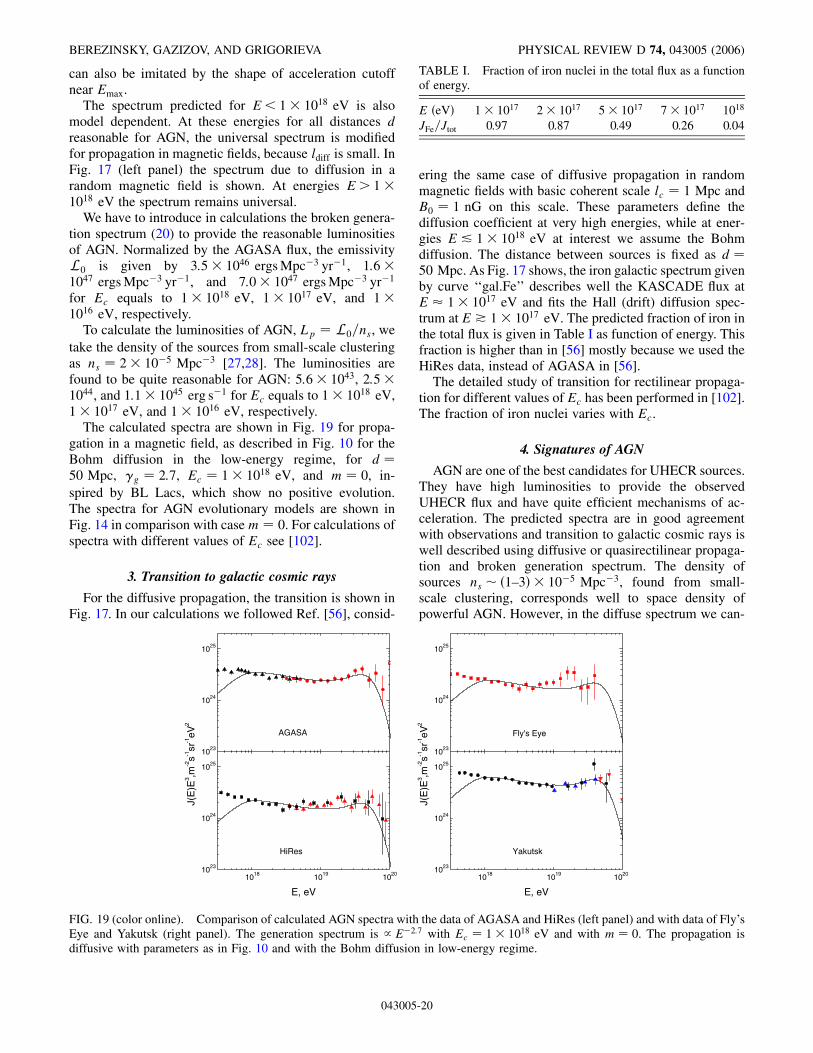
can also be imitated by the shape of acceleration cutoffnear Emax.

The spectrum predicted for E< 1� 1018 eV is alsomodel dependent. At these energies for all distances dreasonable for AGN, the universal spectrum is modifiedfor propagation in magnetic fields, because ldiff is small. InFig. 17 (left panel) the spectrum due to diffusion in arandom magnetic field is shown. At energies E> 1�1018 eV the spectrum remains universal.

We have to introduce in calculations the broken genera-tion spectrum (20) to provide the reasonable luminositiesof AGN. Normalized by the AGASA flux, the emissivityL0 is given by 3:5� 1046 ergs Mpc�3 yr�1, 1:6�1047 ergs Mpc�3 yr�1, and 7:0� 1047 ergs Mpc�3 yr�1

for Ec equals to 1� 1018 eV, 1� 1017 eV, and 1�1016 eV, respectively.

To calculate the luminosities of AGN, Lp � L0=ns, wetake the density of the sources from small-scale clusteringas ns � 2� 10�5 Mpc�3 [27,28]. The luminosities arefound to be quite reasonable for AGN: 5:6� 1043, 2:5�1044, and 1:1� 1045 erg s�1 for Ec equals to 1� 1018 eV,1� 1017 eV, and 1� 1016 eV, respectively.

The calculated spectra are shown in Fig. 19 for propa-gation in a magnetic field, as described in Fig. 10 for theBohm diffusion in the low-energy regime, for d �50 Mpc, �g � 2:7, Ec � 1� 1018 eV, and m � 0, in-spired by BL Lacs, which show no positive evolution.The spectra for AGN evolutionary models are shown inFig. 14 in comparison with casem � 0. For calculations ofspectra with different values of Ec see [102].

3. Transition to galactic cosmic rays

For the diffusive propagation, the transition is shown inFig. 17. In our calculations we followed Ref. [56], consid-

ering the same case of diffusive propagation in randommagnetic fields with basic coherent scale lc � 1 Mpc andB0 � 1 nG on this scale. These parameters define thediffusion coefficient at very high energies, while at ener-gies E & 1� 1018 eV at interest we assume the Bohmdiffusion. The distance between sources is fixed as d �50 Mpc. As Fig. 17 shows, the iron galactic spectrum givenby curve ‘‘gal.Fe’’ describes well the KASCADE flux atE � 1� 1017 eV and fits the Hall (drift) diffusion spec-trum at E * 1� 1017 eV. The predicted fraction of iron inthe total flux is given in Table I as function of energy. Thisfraction is higher than in [56] mostly because we used theHiRes data, instead of AGASA in [56].

The detailed study of transition for rectilinear propaga-tion for different values of Ec has been performed in [102].The fraction of iron nuclei varies with Ec.

4. Signatures of AGN

AGN are one of the best candidates for UHECR sources.They have high luminosities to provide the observedUHECR flux and have quite efficient mechanisms of ac-celeration. The predicted spectra are in good agreementwith observations and transition to galactic cosmic rays iswell described using diffusive or quasirectilinear propaga-tion and broken generation spectrum. The density ofsources ns � �1–3� � 10�5 Mpc�3, found from small-scale clustering, corresponds well to space density ofpowerful AGN. However, in the diffuse spectrum we can-

1023

1024

1025

AGASA

1018 1019 10201023

1024

1025

HiRes

J(E

)E3 ,m

-2s-1

sr-1eV

2

E, eV

1023

1024

1025

Fly's Eye

1018 1019 10201023

1024

1025

Yakutsk

J(E

)E3 ,m

-2s-1

sr-1eV

2

E, eV

FIG. 19 (color online). Comparison of calculated AGN spectra with the data of AGASA and HiRes (left panel) and with data of Fly’sEye and Yakutsk (right panel). The generation spectrum is / E�2:7 with Ec � 1� 1018 eV and with m � 0. The propagation isdiffusive with parameters as in Fig. 10 and with the Bohm diffusion in low-energy regime.

TABLE I. Fraction of iron nuclei in the total flux as a functionof energy.

E �eV� 1� 1017 2� 1017 5� 1017 7� 1017 1018

JFe=Jtot 0.97 0.87 0.49 0.26 0.04


043005-20

not predict any specific signature of AGN, and probablyonly observations of the direct flux of primary (e.g. pro-tons) or secondary (e.g. neutrinos or gamma-rays) radia-tion can give the direct evidence for AGN as sources ofUHECR.

In this respect, the correlations with BL Lacs [30,32] isthe direct indication to AGN as UHECR sources. Theprotons can be the signal carriers. The important point isthat in structured (perforated) magnetic field, there aredirections (holes) with weak magnetic fields in which BLLacs can be seen [91]. In MHD simulation [35], it wasfound indeed that in many large scale structures, like voidsand filaments, the magnetic field is weak and protons canpropagate there with small deflections.

Correlations with BL Lacs imply the jet acceleration,because BL Lacs are AGN with jets directed to an observer.The pinch acceleration mechanism fits well the pictureabove, providing �g � 2:7, high Emax, and high Emin,needed for reasonable luminosity Lp.

C. Gamma ray bursts

GRBs are another candidate for UHECR sources. LikeAGN they have high energy output and can accelerateparticles to UHEs, as has first been proposed in [88–90]

GRB starts with instant energy release Wtot, which oc-curs most probably due to SN explosion. This energy isinjected into a small volume with initial radius Ri � 107

cm in a form of a jet with small opening angle . Theextremely large energy release within a small volumeresults in a very high temperature of the gas, which consistsmostly of photons and electron-positron pairs with a smalladmixture of initially injected baryons. The pressure ofrelativistic ee�� gas accelerates a fireball, its tempera-ture falls down, and the Lorentz factor rises. At later stagesa fireball becomes the baryonic jet moving with Lorentzfactor �0 � Wtot=Mbc

2 � 100, where Mb is initial baryonloading.

The jet is characterized according to observations [103]by small opening angle � 4 and by corresponding solidangle � � �2. The external observer sees only part of theexternal fireball surface within the angle 1=�0 < .Because of this fact, the convenient formalism is to con-sider the fictitious spherically-symmetric fireball withequivalent isotropic energy output Wtot and equivalentisotropic GRB rate �GRB (in units of Mpc�3 yr�1). Thereal energy output and GRB rate are ~Wtot � ��=4��Wtot

and ~�GRB � �4�=��GRB, with the same emissivity L �Wtot�GRB.

According to observations, the equivalent isotropic en-ergy output WGRB � 1� 1053 erg, and spherically-symmetric GRB rate is �GRB � 0:5� 10�9 Mpc�3 yr�1

with emissivity LGRB � 0:5� 1044 erg Mpc�3 yr�1. Themore detailed estimates differ considerably from thisvalue: LGRB � 0:6� 1043 erg Mpc�3 yr�1 (M. Schmidt[104,105]) and LGRB � 1:3� 1044 erg Mpc�3 yr�1 (Frail

et al. [103]). Note, that difference in spectral intervals usedin [103–105] cannot explain alone the differences betweenthe above-cited emissivities. We conclude thus thatLGRB � �0:6–13� � 1043 erg Mpc�3 yr�1, to be comparedwith higher estimate by Waxman [106] LGRB � �3–30� �1043 erg Mpc�3 yr�1.

There are two sites of acceleration in a jet: mildlyrelativistic internal shocks inside a fireball [90] and ultra-relativistic external shock [89].

1. Internal shock acceleration and UHECR

We shall describe here shortly the acceleration insidefireball, following [90,106,107].

Gamma radiation is produced as synchrotron emissionof the shock-accelerated electrons at the stage when thefireball moves with constant Lorenz factor �0 �Wtot=Mbc2. Acceleration occurs due to internal shocksproduced by the motion of fireball subshells with differentLorentz factors �. This phenomenon is assumed to beresponsible for the observed GRBs and for their timesubstructure. In the observer frame the jet looks like anarrow shell with width �� R=�2

0, where R is a radius,i.e. distance from outer surface to the source (the GRBengine). It is assumed that this shell consists of mildlyrelativistic subshells, moving relative to each other in therest frame of the fireball. The inner subshells move fasterthan the outer ones, and their collisions produce mildlyrelativistic shocks. The GRB spikes arise due to shellsubstructure. The range of distances R� where GRB isproduced can be estimated from the observed minimumduration of spikes, �sp * 1 ms, and duration of GRB,�GRB � 1–10 s. Time between collisions of two subshellscan be estimated in the observer frame [107] as t� =v� �2

0 =c, where is the distance between two collid-ing subshells. Thus, R� � c t is limited between Rmin

� �

�20c�sp�3�1011 cm and Rmax

� ��20c�GRB�3�1014–3�

1015 cm. The energetics is described byWGRB � fGRBWtot,with fGRB < 0:5 at least, because half of the total energy isreleased in afterglow. More realistically, fGRB � 0:2.

The exit of all particles from the jet occurs only throughthe front spherical surface, provided by condition >1=�0.

Acceleration of electrons by internal shocks impliesacceleration of protons. According to [90,106], the genera-tion spectrum / E�2, Emax � 1� 1021 eV, Emin �

�0mpc2, and Wp �WGRB (in the observer frame).

As a matter of fact, one must write the expressions aboveas Emin � fa�0mpc

2 and Wp � faWGRB, where fa is afactor of adiabatic cooling. This phenomenon has beenstudied in [108] and adiabatic energy losses were foundto be very severe. As was indicated there the efficientmechanism, which diminishes the influence of adiabaticcooling, is the neutron mechanism of UHECR exit fromexpanding fireball. However, some restrictions obtainedfor this mechanism make its application rather limited.


043005-21

Waxman [106] fought back this criticism by the argumentthat production of HE protons in the shell at later periodscorresponding to a distance Rmax

� eliminates the problem ofadiabatic cooling. We shall argue below that this problemexists.

There are three stages of adiabatic energy losses. Thefirst one occurs during the acceleration process and itoperates at distances Rmin

� &R&Rmax� . The adiabatic en-

ergy losses are described in the standard shock-acceleration equation by the term �p=3� div ~u@�f�r; t; p�=@p, where ~u is hydrodynamical velocity of thegas flow and f�r; t; p� is the distribution function. In ourcase the adiabatic energy losses are large due to expansionof the shell. Adiabatic energy losses diminish the fractionof the shock energy transferred to accelerated particles,which results in the relation Wp � f�1�a WGRB, where f�1�a <1 is the adiabatic factor. Qualitatively it can be explained inthe following way. The first portion of accelerated particleswould suffer severe adiabatic energy losses fa �Rmin� =Rmax

� , if further acceleration were absent. In fact,these particles are reaccelerating and losing energy simul-taneously, as corresponding diffusion equation describes it.This process diminishes only the fraction of energy fatransferred to accelerated particles. It can be estimated asfa � R

eff� =R

max� , but for accurate estimate the solution of

diffusion equation is needed. Unfortunately, this modelexists only in the form of estimates.

The second stage starts after acceleration ceases. Theend of GRB radiation shows this moment. The magneticfield in the expanding shell slowly diminishes, acceleratedelectrons radiate away their energy fast, but protons arestill confined in the shell, forming relativistic gas andlosing energy adiabatically. The duration of this stage isdifferent for protons of different energies and the spectrum/ E�2 is distorted. The protons with 1019–1021 eV are thefirst to accomplish this stage and enter the regime of freeexpansion (stage 3). This energy range is most interestingfor UHECR. The adiabatic factor f�2�a depends on the timeof diminishing of equipartition magnetic field. The detailedcalculations are needed to evaluate f�2�a for the range1019–1021 eV.

At the third stage when the shell of the protons withenergies 1019–1021 eV propagates quasirectilinearly in theexternal magnetic field, the energy losses are also present.They are caused by the collective effect of transferringproton momenta to the macroscopic volume of gas due toscattering in the magnetic field.

As a toy model, let us consider the spherically symmet-ric shell of protons with energies 1019–1021 eV, and makethe order of magnitude estimates. At the distance of orderof gyroradius rL, a proton transfers half of its initial (radial)momentum to the gas. Since protons propagate in the radialdirection almost with light speed, it follows from causalitythat volume of gas, which absorbs the lost momentum,cannot be larger than �r3

L. The equation of radial momen-

tum balance reads

0:5Wp=c� �r3L�gc; (22)

where �g � 10�24 g=cm3 is the density of ambient gas and� is the Lorentz factor obtained by this gas volume. For thespectrum / E�2 the total energy of protons with 1019 E 1021 eV is Wp � 0:2WGRB. For magnetic field in thepresupernova wind at distance r� 1016 cm we accept thevalue of magnetic fieldB0 � 1 G, following the estimate of[99] 0.1–10 G (see also [106]). Then for WGRB � 1�1053 erg we obtain �� 105 and for WGRB � 5� 1050 erg(jet value) �� 103. In fact for the jet case the effectivemass of the target is much less and � is larger. Such gasshell produces the relativistic shock and considered sce-nario is radically changed.

If considered UHE protons capture electrons from themedia with its frozen magnetic field, the pressure of thebeam to the gas further increases.

In fact, we considered above only one mechanism forenergy transfer to the gas. It is clear, that nature of thisphenomenon is very general: the energy density of theproton beam is so large that part of its energy is transferredto magnetized ambient plasma. Only when this densitydrops to some critical value and collective effects disap-pear can the protons propagate as individual particles, notexciting the ambient plasma. Therefore, the total adiabaticfactor fa cannot be of order of 1.

In the left panel of Fig. 20 the calculated flux of UHEprotons accelerated by internal shocks is presented bycurve 1. It corresponds to generation spectrum / E�2

with Emax � 1� 1021 eV and Emin � �0mpc2 �

1� 1011 eV. This is the case of absence of adiabaticenergy losses fa � 1. The spectrum is calculated in thestandard way, taking into account the energy losses onCMB radiation. The emissivity needed to fit the observa-tional data is LCR � 2:2� 1045 erg Mpc�3 yr�1. It mustbe equal to Wp�GRB and thus it should not exceed LGRB

given above. As a matter of fact it is by a factor of 20–300higher. If adiabatic energy losses for protons with energies1019–1021 eV is fa�>1� 1019�, the predicted flux in thisenergy range is additionally suppressed by this factor anddiscrepancy increases correspondingly.

If to assume fa�E 1� 1019eV� � 1, while fa�E �1� 1019 eV� � 1, the energy balance is not changed be-cause the total energy (including Wp and that adiabaticallylost) remains the same.

In the right panel of Fig. 20 we show the spectrum withthe assumed distribution of sources over Emax like in thecase of AGN. In this case the required emissivity is higherLCR � 3:5� 1046 erg Mpc�3 yr�1.

These results have been already presented in [71].Waxman [106] did not understand that we consideredtwo different cases (now being put separately in two differ-ent panels in Fig. 20) and argued in fact only against thecase shown in the right panel of Fig. 20. The left panel


043005-22

shows the same case as considered by Waxman. Ourdiscrepancy in emissivity is explained as follows. Wenormalize our calculations by emissivity Lp (the energyreleased in cosmic ray protons per unit comoving volumeand per unit time) and compare it with LGRB �WGRB�GRB. Waxman normalizes his flux by valueE2 _nCR=dE � 0:8� 1044 erg=Mpc3 yr [106]. To obtainemissivity, this value should be multiplied byln�Emax=Emin�, which is equal to 23 for Emax �1� 1021 eV and Emin � 1� 1011 eV. The obtainedUHECR emissivity roughly agrees with our value, but itexceeds by an order of magnitude what Waxman cites in[106] as the highest value of GRB emissivity (3�1044 erg Mpc�3 yr�1). Note that the comparison is madefor unrealistic case of absence of adiabatic energy losses.

2. External shock acceleration and UHECR

The flow of the ultrarelativistic baryonic jet is termi-nated by the external ultrarelativistic shock propagating inpresupernova wind. The acceleration by such shocks hasbeen described (with relevant references) in Sec. VII B 1.As a shock propagates in interstellar medium, the protons,experiencing the different number of u! d! u cycles,move together with the shock ahead of it (upstream) orbehind it (downstream). The ‘‘fresh’’ particles, whichundergo one or a few (n) cycles have energy E��2

sh2nEi. The ‘‘old’’ particles approach Emax � eBRsh�sh

[93], where Ei is initial proton energy upstream, Rsh is aradius of the shock (the distance from GRB origin), and�sh � 100 is the Lorentz factor of the shock. The accel-eration time ta � E=�ecB�sh� [93] is smaller than the ageof the shock t� Rsh=c for all particles except those withE� Emax.

At this stage of our study we are interested only in thetotal energy transferred to accelerated protons, disregard-

ing what happens to these particles later. In other words weare interested only in energy balance, using the commonassumption Wp �WGRB for the total energy Wp trans-ferred to accelerated protons.

For the typical afterglow distance Rsh � 1016 cm, whenthe shock moves with constant Lorentz factor �sh � 100,we shall use the following parameters for the upstream HEprotons: the power-law spectrum / E��g with the ‘‘stan-dard’’ (see Sec. VII B 1) �g � 2:2, with conservativeEmin � �2

shEi � 1013 eV and with Emax �

eBRsh�sh=��3p� 1� 1021 eV, valid for very large B �

5 G. The fraction of the total energy Wp in the form ofparticles with Ep � 1� 1019 eV is fUHECR � 0:039. Inthe exotic case of the existence of preaccelerated particlesin presupernova wind with Ei � 1013 eV, the minimalenergy is Emin � 1017 eV and fUHECR � 0:29.

As a matter of fact, part of the accelerated particles arelocated downstream. Because they are isotropized in therest frame, the minimum energy in the observer frame isshifted to

Emin �mpc2

2

�sh

�0p�1 �02p =�2

sh�; (23)

where �0p is the Lorentz factor of proton in the rest system.The energy (23) corresponds to a proton moving backwardrelative to shock. Additionally, the number of particleswith maximum energy diminishes due to angular distribu-tion. It results in diminishing of fUHECR; we shall not takethis effect into account.

There is one more effect which diminishes fUHECR fordownstream protons. The highest energy protons can scat-ter to the backward direction and escape through the rearsurface of the shell, while the low-energy protons are betterconfined in the downstream region. In the laboratory framethe backward moving protons have energy about 1 GeV, as

1017 1018 1019 10201023

1024

1025

21

J(E

)E3,

m-2 s

-1 s

r-1 e

V2

E, eV

1017 1018 1019 1020

1024

1025

J(E

)E3,

m-2 s

-1 s

r-1 e

V2

E, eV

FIG. 20 (color online). UHECR from GRBs. In the left panel are shown the fluxes produced by internal shocks (curve 1) withgeneration spectrum / E�2, Emax � 1� 1021 eV and Emin � 1� 1011 eV and by external relativistic shocks (curve 2) with generationspectrum / E�2:2, Emax � 1� 1021 eV and Emin � 1� 1013 eV. In the right panel the spectra are shown with the assumed distributionof sources over Emax, like in the case of AGN. The effective generation spectrum at E> Ec is assumed to be / E�2:7 with Ec �1� 1018 eV.


043005-23

given by Eq. (23). The difference of proton energy (in thelaboratory frame) is transferred to the shell in the processof magnetic scattering. This energy will go back to particleacceleration, and most of it will be taken by low-energyparticles.

Adiabatic energy losses, not taken into account in therelativistic shock acceleration, are discussed in a previoussubsection.

In realistic models, the shock propagates in a diminish-ing magnetic field, e.g. B�R� � B0R0=R [99], valid for thestellar wind. For such a field it is easy to calculate thedeflection angle for proton propagating from Rsh to R,

�eBshRsh

ElnR=Rsh; (24)

and the deflection angle at which the shock overtakes theproton, c �

��3p=�sh, is the same as for constant magnetic

field. The maximum acceleration energy Emax determinedfrom the condition � c remains also approximately thesame. The exit of particles in the interstellar mediumoccurs when �sh diminishes, most notably at the Sedovphase.

In Fig. 20 the calculated spectrum of UHECR fromacceleration by external shock is given by curve 2 for �g �2:2 and Emax � 1� 1021 eV. The UHECR emissivityneeded to fit the flux at E � 1� 1019 eV to the observa-tional data is L�>1� 1019 eV� � 4:7�1044 erg Mpc�3 yr�1. The lower limit to HE proton emis-sivity (without adiabatic energy losses and other effectsdiscussed above) is given by

L p >L�>1� 1019 eV�=fUHECR

� 1:2� 1046 erg Mpc�3 yr�1 (25)

for Emin � 1� 1013 eV, and Lp > 1:6�1045 erg Mpc�3 yr�1 for the exotic case with Emin � 1�1017 eV. The emissivity (25) is 2–3 orders of magnitudeshigher than the observed GRB emissivity �0:6–13� �1043 erg Mpc�3 yr�1. The exotic assumption of Emin �1� 1017 eV reduces this discrepancy only by 1 order ofmagnitude.

3. Discussion and conclusion

The calculations above agree with earlier works[71,72,109,110] (note the emissivities given in the lastwork of this list).

The main difference between calculations[71,72,109,110]) on the one hand, and those by Waxman(e.g. [106]) and Vietri (e.g. [99]), on the other hand, con-sists of the following.

While Waxman and Vietri compare GRB emissivitywith emissivity of the observed UHECR (Vietri at E �1� 1017 eV), we compare it with emissivity, which cor-responds to energy transferred to all protons in the processof their acceleration. Apart from spectral fraction of en-

ergy, it includes also the energy lost by protons before theyescape to extragalactic space (adiabatic energy losses,energy transferred to the magnetized plasma outside thejet, and others discussed above). Waxman for UHECRenergy input uses the value E2d _nCR=dE � 0:8�1044 erg Mpc�3 yr�1 [106], which after integration fromEmin � 1� 1011 eV to Emax � 1� 1021 eV correspondsto emissivity Lp � 1:8� 1045 erg Mpc�3 yr�1 to be com-pared with the observed GRB emissivity �0:6–13� �1043 erg Mpc�3 yr�1. Because of adiabatic energy losses,Lp is expected to be, in fact, much higher than the above-mentioned value.

Vietri et al. [99] indicate UHECR energy release re-quired by observations as 1� 1045 erg Mpc�3 yr�1 forenergy interval 1� 1017–1� 1021 eV (compared withour value 1:6� 1045 erg Mpc�3 yr�1 for the same energyinterval). If one includes the energy input to all acceleratedprotons, which accompany ultrarelativistic shock, fromEmin � �2

shEi to Emax, this emissivity increases at least bya factor of 7.3, in conflict with observations by a factor of60. There is some difference with our work in numericalcalculations: Vietri et al. uses the HiRes data, we energy-shifted data by AGASA and HiRes, which are in goodintrinsic agreement (see Fig. 20); Vietri et al. introducecorrections due interaction fluctuations, we do not need todo it because we normalize our calculations by observa-tional data at E � 2� 1019 eV, where fluctuations areabsent. The maximum acceleration energy Emax �1� 1021 eV at Rsh � 1� 1016 eV requires according toour calculations (it is by factor

��3p

less than in [93]) amagnetic field in the presupernova wind at this distance�6 G, which is very large and marginally possible only forthe SupraNova model [111,112].

Our calculations require the UHECR emissivityL�>1� 1019 eV� � 4:4� 1044 erg Mpc�3 yr�1 for inter-nal shock acceleration (�g � 2:0 and Emax � 1�1021 eV) and 4:7� 1044 erg Mpc�3 yr�1 for external ul-trarelativistic shock acceleration (�g � 2:2 and Emax �

1� 1021 eV). Including the energy injected in low energyprotons (not necessarily coming outside), this emissivityshould be minimum 10–30 times higher, and thus contra-diction with GRB emissivity reaches conservatively thefactor 30–100. A natural solution to this problem is givenby an assumption that accelerated protons carry �100times more energy than electrons, whose radiation is re-sponsible for GRBs. However, for 4 beaming it increasesthe required energy output of SN as GRB source fromWSN � 5� 1050 erg to 1052–1053 erg, which creates theserious problem for SN models of GRBs. This problemexists even for the case when one takes into account only‘‘observed’’ UHECR emissivity L�>1� 1019 eV�. Thenthe minimal energy balance for the internal shock modelincludes LGRB � 1:3� 1044 erg Mpc�3 yr�1, Lafterglow �

LGRB, L�>1� 1019 eV�, and L� � L�>1� 1019 eV�,which results in SN energy output 4� 1051 erg. For the


043005-24

external shock model the energy balance does not includeneutrinos and it results in WSN � 3� 1051 erg.

VIII. CONCLUSIONS

This work is naturally subdivided into two major parts:(i) the model-independent analysis of spectral signatures ofUHE proton interaction with the CMB and (ii) the model-dependent analysis of the transition from extragalactic togalactic cosmic rays and model-dependent study of mostprobable UHECR sources: AGN and GRBs.

In the first part, the number of assumptions is minimal:we assume the power-law generation spectrum of extra-galactic protons / E��g and analyze uniform distributionof the sources with a possible distortion in the form oflarge-scale source inhomogeneities and local overdensityor deficit of the sources. The reference spectrum is givenby the universal spectrum, calculated for the homogeneousdistribution of the sources, when separation of sources d!0. According to the propagation theorem [53], in this casethe spectrum does not depend on the propagation mode,e.g. it is the same for rectilinear and diffusive propagation.We analyze also the spectra with different source separa-tions, giving emphasis to separations d� 30–50 Mpc, fa-vorable by clustering of UHECR [26–28].

Calculation of the universal spectrum is based on anequation of conservation of particles with continuous en-ergy losses of protons interacting with the CMB. Weperformed the new calculations of energy losses (firstpresented in [71]), which agree well with [50,57], seeFig. 1. The technical element needed for calculations, theratio of energy intervals at generation and observationdEg=dE, is calculated by the new method (seeAppendix B). The analysis of spectral features is conve-nient to perform with help of a modification factor, ��E� �Jp�E�=Junm

p �E�, where the spectrum Jp�E� is calculatedwith all energy losses included, and the unmodified spec-trum Junm

p �E�—only with account of adiabatic energylosses (redshift).

There are four major signatures of UHE protons inter-acting with CMB: GZK cutoff, bump, dip, and the seconddip.

GZK cutoff [8,9] is the most prominent signature, whichconsists of the steepening of the proton diffuse spectrumdue to photopion production. The beginning of the GZKcutoff at EGZK � 4� 1019 eV is difficult to observe. Thequantitative characteristic of the GZK cutoff is given byenergy E1=2, where the flux with the cutoff becomes lowerby a factor of 2 in comparison with power-law extrapola-tion from lower energies. This quantity is possible toobserve only in an integral spectrum. Practically indepen-dent of �g, E1=2 � 5:3� 1019 eV. Data of Yakutsk andHiRes are compatible with this value (see Fig. 4), whiledata of AGASA contradict it. As to spectral shape of theGZK cutoff, we found it very model dependent: it dependson separation of sources d, on local source overdensity or

deficit, on maximum acceleration energy Emax, and beingso uncertain, the GZK steepening can be imitated by Emax

acceleration steepening.Bump is produced by pileup protons, experiencing the

GZK process. These protons do not disappear, they onlyshift in energy towards that where the GZK cutoff begins.The bump is very clearly seen in the spectra of individualsources (see left panel of Fig. 7), but they disappear in thediffuse spectrum (right panel of Fig. 7) because individualbumps are located at different energies.

Dip is the most robust signature of UHE protons inter-acting with the CMB. It has a very specific shape (seeFig. 2), which is difficult to imitate by other processes,unless one has a model with many free parameters. Dip isproduced by pair production on the CMB photons p�! p e e� and is located in energy interval 1�1018–4� 1019 eV. Dip has two flattenings (see Fig. 2), oneat energy E� 1� 1019 eV, which automatically reprodu-ces the ankle, well seen in the observational data (seeFig. 8), and the other at E� 1� 1018 eV, which providesthe transition from extragalactic to galactic cosmic rays.The prediction of the dip shape is robust. It is not notice-ably modified by many phenomena included in calcula-tions: by different distances between sources (Fig. 9), bychanging the rectilinear propagation of protons to thediffusive (Fig. 10), by different Emax (Fig. 5), by localoverdensity and deficit of the sources (Fig. 6), by large-scale source inhomogeneities and fluctuations inp�-interactions (Fig. 15).

The dip is very well confirmed by data of Akeno-AGASA, HiRes, Yakutsk, and Fly’s Eye (see Fig. 19 forthe latter), while data of Auger at this stage do not contra-dict the dip (Fig. 8). The agreement with the data of eachexperiment Akeno-AGASA, HiRes, and Yakutsk is char-acterized by �2 � 19–20 for about 20 energy bins, andwith only two free parameters, �g and the flux normaliza-tion constant. The best fit is reached at �g � 2:7, with theallowed range 2.55–2.75.

The dip is used for energy calibration of the detectors,whose systematic energy errors are up to 20%. For eachdetector independently the energy is shifted by factor � toreach the minimum �2. We found �Ag � 0:9, �Hi � 1:2,and �Ya � 0:75 for AGASA, HiRes, and Yakutsk detec-tors, respectively. Remarkably, after this energy shift, thefluxes and spectra of all three detectors agree perfectly,with discrepancy between AGASA and HiRes at E> 1�1020 eV being not statistically significant (see Fig. 11). TheAGASA excess over predicted GZK cutoff might have thestatistical origin combined with systematic errors in energydetermination, and the GZK cutoff may exist.

The difference in energy shifts between fluorescent en-ergy measurement (HiRes) and on-ground measurements(AGASA, Yakutsk) with � > 1 for HiRes and � < 1 forAGASA and Yakutsk may signal a systematic difference inenergy determination by these two methods.


043005-25

The excellent agreement of the dip with observationsshould be considered as a confirmation of UHE protoninteraction with the CMB.

For astrophysical sources of UHECR, the presence ofnuclei in primary radiation is unavoidable. Whatever asource is, the gas in it must contain at least helium ofcosmological origin with ratio of densities nHe=nH �0:079. Any acceleration mechanism operating in this gasmust accelerate helium nuclei, if they are ionized. Thefraction of helium in the primary radiation depends criti-cally on the mechanism of injection. Figure 13 shows thatwhile 10% mixing of helium with hydrogen in the primaryradiation leaves good agreement of dip with observations,20% mixing upsets this agreement. One may conclude thatgood agreement of dip with observations indicates a par-ticular acceleration mechanism, more specifically an injec-tion mechanism. One may also note that the shape of thedip contains the information about the chemical composi-tion of primary radiation (see Fig. 12).

The low-energy flattening of the dip is seen for bothrectilinear and diffusive propagation (see Fig. 16). It isexplained by the transition from adiabatic energy lossesto that due to ee�-pair production. Low-energy flatteningof the extragalactic spectrum provides transition to a moresteep galactic component, as one can see it in the left panelof Fig. 17. Note, that when the spectrum is multiplied toE2:5 the flat spectrum looks like one raising with energy. InFig. 17 the transition is shown for the diffusive spectrum.This model of transition implies that at energy below Etr �5� 1017 eV the galactic iron is the dominant component,while at the higher energy extragalactic protons with someadmixture of extragalactic helium dominate. The observa-tional spectrum feature, which corresponds to this transi-tion, is the second knee. The prediction of this model, thedominance of proton component at E> 1� 1018 eV, isconfirmed by data of HiRes [13,14], HiRes-MIA [15], byYakutsk [16] and does not contradict to the Haverah Parkdata at E> �1–2� � 1018 eV [1]. However, the Akeno [17]and Fly’s Eye [5] data favor the mixed composition domi-nated by heavy nuclei.

The second dip is produced by interplay between pairproduction and photopion production. It is a narrow featureat energy E2dip � 6:3� 1019 eV, which can be observedby detectors with good energy resolution. If detected, itgives the precise mark for energy calibration of a detector.

The UHECR sources have to satisfy two conditions:they must be very powerful and must accelerate particlesto Emax � 1� 1021 eV. There is one more restriction [22–28], coming from the observation of small-scale clustering:the space density of the sources should be �1–3� �10�5 Mpc�3, probably with noticeable uncertainty in thisvalue. Thus, these sources are more rare, than typicalrepresentatives of AGN, Seyfert galaxies, whose spacedensity is �3� 10�4 Mpc�3. The sources could be therare types of AGN, and indeed the analysis of [30] shows a

statistically significant correlation between directions ofparticles with energies �4–8� � 1019 eV and directions toAGN of the special type—BL Lacs. The acceleration inAGN can provide the maximum energy of acceleration toEmax � 1021 eV. The appropriate mechanisms can be ac-celeration by relativistic and ultrarelativistic shocks (seeSec. VII B 1). These mechanisms typically provide spectraflatter than one with �g � 2:6–2:8, needed for agreementof the dip with data. The distribution of the sources overEmax suggested in [28] solve this problem: starting fromsome energy Ec the spectrum becomes steeper. In this casethe diffuse spectrum below Ec has a canonical generationindex �g � 2:0 or �g � 2:2, and above this energy �g �2:6–2:8 to fit the observations. The energy Ec is a freeparameter of the models, and we keep it typically as1017–1018 eV. Such broken generation spectrum relaxesthe requirements for source luminosities. For example, for�g � 2:7 and Ec � 1� 1018 eV, the typical emissivityneeded to fit the observed flux is L0 � nsLp � 3�1046 erg Mpc�3 yr�1, which is held for the source densityns � 2� 10�5 Mpc�3, estimated from the small-angleclustering [27,28], and for the source luminosity Lp � 6�1043 erg=s, very reasonable for AGN. The calculated spec-tra are in a good agreement with observations (see Fig. 19).The transition from galactic to extragalactic cosmic rays inthis model occur at the second knee (see left panel ofFig. 17).

GRBs are another potential UHECR source. They havelarge energy output and can accelerate particles to UHEs.Acceleration occurs at the multiple inner shocks [90,113]and at ultrarelativistic external shock [89,99]. The maxi-mum acceleration energy can be as high as�1� 1021 eV.In the case of ultrarelativistic shock with a Lorentz factorof shock �sh � 100 and at distance Rsh � 1� 1016 cm,typical for afterglow region, the maximum energy Emax �

�1=��3p�eBRsh�sh reaches 1� 1021 eV in the case of a very

strong external magnetic field B� 6 G. Such a strongmagnetic field can be marginally provided by two com-bined effects: a strong field in presupernova wind (possibleonly in the model of SupraNova [111,112]) combined withpreshock amplification of the field.

The energy output of GRBs necessary to provide theobserved UHECR flux imposes a serious problem[71,72,109,110]. It is usually assumed that energy outputin the form of accelerated protons is an order of magnitudeof that observed in GRB photons. The observed emissivityof GRBs is

L � �0:6–13� � 1043 erg Mpc�3 yr�1; (26)

where the lower value is from works by Schmidt [104,105]and the large value from work by Frail et al. [103]. Bothauthors used in their estimates the similar energy intervalof photons, (10–1000 keV) and (0.2–2000 keV).

Our calculations of UHECR spectra for internal shocks(see Fig. 20 curve 1) with �g � 2:0 and Emax�1�1021 eV


043005-26

give UHECR emissivity L�� 1� 1019 eV� � 4:4�1044 erg Mpc�3 yr�1, by factor 3.4–73 higher than (26).If to include the L� �LUHECR contradiction with (26)increases to 6.8–150. If to include in balance the protonswith energies down to Emin � 1� 1011 eV (not necessarilycoming out), the contradiction increases by another factor5. Adiabatic energy losses further increase thisdiscrepancy.

Our calculations for external shock acceleration (seecurve 2 in Fig. 20) with �g � 2:2 and Emax � 1�1021 eV results in UHECR emissivity L�� 1�1019 eV� � 4:7� 1044 erg Mpc�3 yr�1, i.e. by a factor3.6–78 times higher than (26). It increases by a factor of26, if to include protons with energies down to Emin ��2

shEi � 1013 eV, or by a factor of 3.5 for the unrealisticcase of Emin � 1� 1017 eV. Adiabatic energy losses areless than in the case of internal shock acceleration.

This energy crisis can be resolved, assuming that accel-erated protons in GRBs take away �100 times moreenergy than electrons responsible for GRB photons.However, this assumption dramatically affects the statusof the SN origin for GRBs, even in the case of narrow 4

beaming.

Predictions for the Auger measurements

What do we predict for the Auger observations on thebasis of our analysis?

(i) We predict the dip at energy 1� 1018–4�1019 eV not only as the spectrum shape, butwith the absolute values of flux, based on theagreement of AGASA-HiRes-Yakutsk fluxes after

energy calibration by the dip (see Fig. 11). Thisspectrum is displayed in the left panel of Fig. 21.The distortion of the shape of the predicted spec-trum can occur only due to the presence of extra-galactic nuclei.

(ii) The above-mentioned distortion is important asa tool for measuring the chemical compositionof UHECR. The chemical composition is themost difficult problem for UHECR experiments,in which little progress has been reached dur-ing the last 30 years. The measurement of thedip shape gives the precise method of determina-tion of 10%–15% of admixture of helium inprimary UHECR (see Fig. 12). The distortion ofthe proton dip most noticeably occurs at energyE * 3� 1019 eV, (see Fig. 13) where precisemeasurements of Auger are expected.

(iii) Normalization of energies measured by AGASA,Yakutsk and HiRes detectors with the help of thedip (see Sec. IV C) implies that energy measuredby fluorescent method is higher than that by on-ground method (the energy shift for AGASA andYakutsk is � < 1, while for HiRes � > 1). Withhelp of the hybrid events Auger can resolve thisproblem.

(iv) The second dip (see Fig. 24) may be marginallyobserved and used for energy calibration of thedetector.

(v) Yakutsk and HiRes data give evidence for thenumerical characteristic of the GZK cutoffE1=2 �5:3� 1019 eV in the integral spectrum (see

1017 1018 1019 1020 102110-8

10-7

10-6

10-5

10-4

10-3

10-2

10-1

200

500

1000

100

5030

r=10 Mpc

J(E

) E

γ g, arb

. units

E, eV

FIG. 21 (color online). Predictions for the Auger detector. In the left panel the diffuse spectrum prediction is displayed for differentdistances d between sources, which provide the largest uncertainties. The spectrum is normalized by the energy-shifted AGASA datawhich coincides well with HiRes and Yakutsk data (see Fig. 11). In energy range 1� 1018–7� 1019 eV, the uncertainties in thepredictions are small and Auger should observe the beginning of the GZK cutoff at E � 5� 1019 eV. In the right panel the spectrawith bumps from the nearby sources are displayed (�g is the generation index).


043005-27

Fig. 4). In the Auger data this value can be mea-sured more reliably.

(vi) The predicted shape of the GZK steepening hasmany uncertainties (see Sec. III A for the discus-sion). However, the beginning of the GZK cutoffin the narrow energy interval �4–7� � 1019 eV ispredicted with the high accuracy (see left panel inFig. 21). The precise spectrum measurement inthis energy range can give the decisive proof ofthe GZK cutoff.

(vii) The mass composition at 1� 1018 & E &

1� 1019 eV measured by the fluorescent tech-nique can distinguish between models of thesecond-knee transition from galactic to extraga-lactic cosmic rays (protons with 10%–20% ofhelium) and the ankle transition (iron dominance)

(viii) The bumps in the spectrum of single sources, ifdetected, can be observed (see Fig. 21).

ACKNOWLEDGMENTS

We acknowledge the participation of R. Aloisio and P.Blasi in some parts of this work. B. Hnatyk, D. De Marcoand M. Kachelriess are thanked for useful discussions.Participation of M. I. Levchuk at the initial stage of pair-production energy loss recalculation is gratefully acknowl-edged. We thank ILIAS-TARI for access to the LNGSresearch infrastructure and for the financial supportthrough EU Contract No. RII3-CT-2004-506222. Thework of S. G. is partly supported by Grant No. LSS-5573.2006.2.

APPENDIX A: CALCULATIONS OF ENERGYLOSSES

We consider here some details of calculations of energy-losses due to production of ee�-pairs and pions.

Pair production energy loss of ultrahigh energy protonsin low-temperature photon gas, e.g. CMB,

p �CMB ! p e e�; (A1)

has been previously discussed in many papers. The differ-ential cross-section for this process in the first Born ap-proximation was originally calculated in 1934 by Betheand Heitler [114] and Racah [115]. In 1948 Feenberg andPrimakoff [116] obtained the pair production energy lossrate using the extreme relativistic approximation for thedifferential cross-section. In 1970 the accurate calculationwas performed by Blumenthal [39]. Later some analyticalapproximations to differential cross-sections were ob-tained in Ref. [117].

All authors neglected the recoil energy of proton, puttingmp ! 1, the effect being suppressed by a factor ofme=mp � 5� 10�4.

In spite of the fact that all calculations actually used thesame Blumenthal approach, there are noticeable discrep-

ancies in the results of different authors; they are displayedin Fig. 1b of Ref. [51].

To clarify the situation we recalculate the pair produc-tion energy loss of high-energy proton in the low-temperature photon gas. In contrast to Ref. [39], we usethe first Born approximation approach of Ref. [40] takinginto account the finite proton mass. The exact nonrelativ-istic threshold formula with corrections due to differentCoulomb interactions of electron and positron with theproton (see e.g. Ref. [118]) is used. No series expansionsof ��"r�, where "r is the photon energy in the proton restsystem, are involved in our calculations. The averagefraction of proton energy loss in one collision with aphoton is defined as

h1� xi�"r� �1

��"r�

Z xmax�"r�

xmin�"r�dx�1� x�

d��"r; x�dx

; (A2)

where x � E0p=Ep, with Ep and E0p being the incident andfinal proton energies, respectively, in the laboratory sys-tem. The upper and lower limits on fractions x are given by

xmaxmin�"r� � xc�"r� � yc�"r�; (A3)

xc�"r� �1

2

�1

m2p �m2

�

m2p 2mp"r

�;

yc�Ec� �

��x2c�"r� �

m2p

m2p 2mp"r

vuut :

(A4)

Our strategy was to calculate h1� xi�"r� by performingthe direct fourfold integration of the exact matrix elementover the phase space. It should be noted, that direct nu-merical integration, especially at high energies, is difficultin this case because of forward-backward peaks in theelectron-positron angular distributions. To overcome thisproblem, we performed two integrations over polar andazimuth angles in the ee� subsystem analytically. Thiswas facilitated by using the MATHEMATICA 4 code. Theresidual two integrations over energy and scattering anglein the initial p� subsystem were carried out numerically.We calculate simultaneously the total cross-section for pairproduction. The accuracy of our calculations was thuscontrolled by comparison of the calculated total cross-section with the well-known Bethe-Heitler cross-section.

The average fraction of proton energy lost in one colli-sion with a photon is plotted in Fig. 22 as a function of thephoton energy in the proton rest system.

The product of this fraction and the total cross-sectionfor pair production is shown in Fig. 22. This functionshould be integrated over the photon spectrum to obtainthe average energy loss due to pair production in thephoton gas with this spectrum.

The comparison of our calculations with Ref. [51] showsthe negligible difference (see Fig. 1).


043005-28

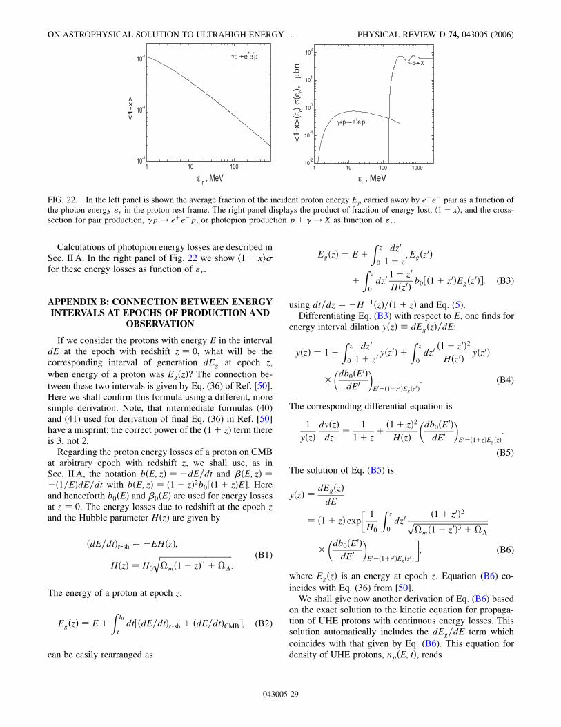
Calculations of photopion energy losses are described inSec. II A. In the right panel of Fig. 22 we show h1� xi�for these energy losses as function of "r.

APPENDIX B: CONNECTION BETWEEN ENERGYINTERVALS AT EPOCHS OF PRODUCTION AND

OBSERVATION

If we consider the protons with energy E in the intervaldE at the epoch with redshift z � 0, what will be thecorresponding interval of generation dEg at epoch z,when energy of a proton was Eg�z�? The connection be-tween these two intervals is given by Eq. (36) of Ref. [50].Here we shall confirm this formula using a different, moresimple derivation. Note, that intermediate formulas (40)and (41) used for derivation of final Eq. (36) in Ref. [50]have a misprint: the correct power of the (1 z) term thereis 3, not 2.

Regarding the proton energy losses of a proton on CMBat arbitrary epoch with redshift z, we shall use, as inSec. II A, the notation b�E; z� � �dE=dt and ��E; z� ��1=E�dE=dt with b�E; z� � �1 z�2b0��1 z�E�. Hereand henceforth b0�E� and �0�E� are used for energy lossesat z � 0. The energy losses due to redshift at the epoch zand the Hubble parameter H�z� are given by

�dE=dt�r-sh � �EH�z�;

H�z� � H0

��m�1 z�3 ��

q:

(B1)

The energy of a proton at epoch z,

Eg�z� � EZ t0

tdt��dE=dt�r-sh �dE=dt�CMB�; (B2)

can be easily rearranged as

Eg�z� � EZ z

0

dz0

1 z0Eg�z0�

Z z

0dz0

1 z0

H�z0�b0��1 z0�Eg�z0��; (B3)

using dt=dz � �H�1�z�=�1 z� and Eq. (5).Differentiating Eq. (B3) with respect to E, one finds for

energy interval dilation y�z� � dEg�z�=dE:

y�z� � 1Z z

0

dz0

1 z0y�z0�

Z z

0dz0�1 z0�2

H�z0�y�z0�

�

�db0�E0�dE0

�E0��1z0�Eg�z0�

: (B4)

The corresponding differential equation is

1

y�z�dy�z�dz�

1

1 z�1 z�2

H�z�

�db0�E

0�

dE0

�E0��1z�Eg�z�

:

(B5)

The solution of Eq. (B5) is

y�z� �dEg�z�

dE

� �1 z� exp�

1

H0

Z z

0dz0

�1 z0�2��m�1 z0�3 ��

p�

�db0�E0�dE0

�E0��1z0�Eg�z0�

�; (B6)

where Eg�z� is an energy at epoch z. Equation (B6) co-incides with Eq. (36) from [50].

We shall give now another derivation of Eq. (B6) basedon the exact solution to the kinetic equation for propaga-tion of UHE protons with continuous energy losses. Thissolution automatically includes the dEg=dE term whichcoincides with that given by Eq. (B6). This equation fordensity of UHE protons, np�E; t�, reads

ε r

1 10 100 100010

-2

10-1

100

101

102

γ+p e+e-p

εr , MeV

γ+p X

<1-x

>(ε

r) σ

(εr),

µb

n

FIG. 22. In the left panel is shown the average fraction of the incident proton energy Ep carried away by ee� pair as a function ofthe photon energy "r in the proton rest frame. The right panel displays the product of fraction of energy lost, h1� xi, and the cross-section for pair production, �p! ee�p, or photopion production p �! X as function of "r.


043005-29

@@tnp�E; t� �

@@E�~b�E; t�np�E; t�� Qg�E; t� � 0; (B7)

with ~b�E; t� � EH�t� b�E; t�, where EH�t� describesadiabatic energy loss and b�E; t�—those due to interactionwith the CMB.

Written in the equivalent form

@@tnp�E; t� � ~b�E; t�

@@E

np�E; t�

� np�E; t�@~b�E; t�@E

�Qg�E; t� � 0; (B8)

this equation can be solved with help of auxiliary charac-teristic equation dE=dt � �~b�E; t�, which solution isE�t� � Eg�Ei; ti; t�, where like in Sec. II B Eg is the gen-eration energy at age t, if E � Ei at ti. When the energy ofa proton is taken on the characteristic E � E�t�, the secondterm in the left-hand side of Eq. (B8) disappears and thesolution found with help of integration factor is

np�E; t� �Z t

tmin

dt0Qg�E�t0�; t0�

� exp�Z t

t0dt00

@@Eb�E�t00�; t00�

�: (B9)

Introducing the redshift z as a variable, dt=dz ��H�1�z�=�1 z�, we obtain for present epoch (z � 0):

np�E� �Z zmax

0

dz0

�1 z0�H�z0�Qg�E�z

0�; z0�

� exp�Z z0

0

dz00

�1 z00�H�z00�@b�E; z00�@E

�(B10)

Using

@b�E; z�@E

� H�z� �1 z�3�@b0�E

0�

@E0

�E0��1z�E�z�

one finally gets

np�E� �Z zmax

0

dz0

�1 z0�H�z0�Qg�E�z0�; z0��1 z0�

� exp�

1

H0

Z z0

0dz00

�1 z00�2��m�1 z00�3 ��

p�

�@b0�E

0�

@E0

�E0��1z00�E�z00�

�(B11)

Since E�z0� � Eg�z0�, one easily recognizes inside the

integral the term dt0Qg�Eg; t0� and dEg=dE as given byEq. (B6).

APPENDIX C: KINETIC EQUATION SOLUTION VSCONTINUOUS LOSS APPROXIMATION:

PHYSICAL INTERPRETATION

We shall compare here the kinetic equation solution forproton spectra, nkin�E�, with that obtained in continuous-

energy-loss (CEL) approximation, ncont�E�, and study thephysical meaning of their difference.

In addition to the full kinetic equation (16), we shallconsider here also the stationary kinetic equation with thephotopion production only. Such equation describes real-istically the spectrum at E> 1� 1020 eV, where pionenergy losses dominate, and the effects of CMB evolutionare negligible. However, we formally consider this equa-tion at the lower energies, too, to study the differencebetween kinetic equation solution and CEL approximation.

The general kinetic equation is reduced to the stationaryone with photopion interaction only, putting in Eq. (16)@n=@t � 0, H�t� � 0, T � T0 and bpair � 0.

Then the stationary kinetic equation reads

� P�E�np�E� Z Emax

EdE0P�E0; E�np�E

0� Qgen�E� � 0;

(C1)

with P�E� and P�E0; E� given by Eqs. (17) and (18).Introducing variable x � E=E0, we rearrange the regenera-tion term into

1

E

Z 1

0dx�Ex

�P�E=x; x�np�E=x�: (C2)

Expanding the integrand into the Taylor series in powers of(1� x) one observes the exact compensation of the zeropower term with �P�E�n�E�. The first power term resultsin the stationary continuous energy loss equation

@@E�b�E�np�E�� Qgen�E� � 0; (C3)

and account of �1� x�2 term gives the stationary Fokker-Planck equation

@@E

�b�E�np�E�

@@E�E2D�E�np�E��

�Qgen�E� � 0;

(C4)

where the term with diffusion coefficient D�E� in momen-tum space describes fluctuations.

This result reproduces the general proof (see e.g. [75],p. 89) for the case when all processes go with a smallenergy transfer.

Let us now consider the analytic solution to Eq. (C1)with Emax ! 1 in the asymptotic limit E� EGZK. Weshall use here (and only here) a toy model with simplifiedassumptions about interactions, namely, with one-pionproduction p �! � N, with isotropic pion distribu-tion in c.m. system and with asymptotic cross-section�p� ! const, when Ec ! 1. With these assumptions wereadily obtain

P�E� ! c�p�n�; P�E0; E� ! c�p�n�=E0; (C5)

and using Qgen�E� � Q0E��g , we arrive at


043005-30

nkin�E� ��g

�g � 1

1

�p�n�cQ0E��g : (C6)

For the continuous energy loss equation (C3), usingb�E0� � hE0 � Eic�p�n� and hE0 � Ei � 1

2E0, valid for

isotropic pion distribution in c.m. system, we obtain

ncont�E� �2

c�p�n�Q0E

��g : (C7)

Therefore, the asymptotic ratio is

nkin�E�ncont�E�

��g2; (C8)

valid also for �g � 2. This result has been obtained earlierin [119]. Of course, at the considered energies nothing butfluctuations are responsible for ratio (C8). This ratio, beingasymptotic, can be used, however, as an estimate of role offluctuations at E� EGZK.

Let us now come over to the case of finite Emax andconsider E very close to Emax.

The regeneration term in Eq. (C1) tends to zero and

nkin�E� !Q0E

��gmax

P�Emax�; (C9)

having nonzero value at E � Emax � � and being zero atE � Emax �, where � is infinitesimally small energy.

For particle density at E � Emax � � in continuous lossapproximation one obtains from Eq. (C3)

ncont�Emax� �1

b�Emax�

Z Emax

Emax�EQ0E��gdE�

�Emax

! 0:

(C10)

Therefore, nkin�E�=ncont�E� ! 1 as E! Emax.This result has a clear physical meaning. In our model

sources are homogeneously distributed and from nearbysources the particles with energy Emax can arrive at theobservational point with the same energy due to fluctua-tions. But in CEL approximation they cannot do it, sincethey loose energy at any distance traversed, whatever smallit is. The described effect influences the ratio r�E� �nkin�E�=ncont�E� at all energies close enough to Emax.

Let us now come over to the solution of Eq. (C1) withinteraction given by the detailed calculations as describedin Sec. V. The calculated ratio r�E� � nkin�E�=ncont�E� isplotted in Fig. 23 for Emax � 1� 1023 eV and for threevalues of �g equal to 2.3, 2.7, and 2.9. One may observe inFig. 23 some features described by our toy model: the ratior�E� increases with �g as it should according to Eq. (C8)and it tends to 1 at Emax. For spectra of interest for thepresent work with 2:3 & �g & 2:8, the ratio r�E� at 1�1019 E 1� 1021 eV does not exceed 10%. Note thatin Fig. 15 it is smaller at low energies because the non-fluctuating pair-production process is included there.

The ratio of the solutions for the kinetic equation and forthe CEL equation includes fluctuations, but it includes alsosome other effects. The kinetic equation tends to the CELequation (C3) in the limit of small 1� x. But in fact for allreasonable energies, 1� x is limited by minimum valuem�=�m� mp� � 0:13, which cannot be considered as asmall value for the discussed accuracy. The same argumentis valid for comparison of the Monte-Carlo simulation withthe CEL approximation: why they should coincide if theenergy transfer process is discrete? However, we do seefrom Fig. 23 that the ratio r�E� differs from 1 just by a fewpercent, when energy becomes less than 1� 1019 eV.

Appendix D gives an example when kin/CEL ratio atenergy close to 1� 1020 eV is explained not by fluctua-tions. At energy E � 6� 1019 eV the kin/CEL ratio isaffected by an interplay between pair- and photopionproduction.

We shall now discuss the comparison of our calculationswith Monte-Carlo (MC) simulations.

As was emphasized in Sec. V the kinetic equationsolution must coincide exactly with MC simulation whenthe number of the MC tests tends to infinity, the distribu-tion of sources is homogeneous, �g and Emax are the sameand interactions are included in the identical way. D. DeMarco and M. Kachelriess run their MC programs spe-cially for comparison with our calculations using �g �2:7, Emax � 1� 1023 eV and homogeneous distributionof sources. They used the SOPHIA interaction model[51], which is not identical to our interaction model espe-cially at the highest energies E � 1� 1021 eV, but theaverage energy losses coincide well in both models (seeFig. 1). The comparison of MC/CEL and kin/CEL ratiosare given in the Table below. The data of MC are kindlyprovided by D. De Marco (D) and M. Kachelriess (K).

From Table II one can see the tendency of smaller kin/CEL ratios in comparison with MC/CEL, which can be due

1019 1020 1021 1022 10230.9

1.0

1.1

1.2

1.3

1.4

1.5

γg=2.9

nkin. eq

(E,γg)/n

cont(E,γ

g)

2.32.7r(E

, γg)

E, eV

FIG. 23. Ratio of solutions of the kinetic equation (C1) andCEL Eq. (C3) for Emax � 1� 1023 eV as a function of energy incase of realistic p�-interaction and for different values ofgeneration indices �g, shown by numbers on the curves.


043005-31

to different interaction models used in these calculations.We are planning the joint work with D. De Marco and M.Kachelriess on the detailed study of the discussed effectsby methods of kinetic equation and Monte-Carlo.

The main conclusion of our study is that fluctuations inphotopion production modify only weakly the spectra withdifferent �g at energies up to 1� 1021 eV (see Fig. 23).

APPENDIX D: THE SECOND DIP

As explained qualitatively in Sec. III D the second dipappears due to the breaking of the compensation betweenparticle exit and regeneration given by the first and secondterms in Eq. (C1). This is a narrow feature near the energyEeq2 which is produced because of the sharp (exponential)increase of photopion energy losses with energy, seen inFig. 1. At energy E just slightly below Eeq2 the continuous(adiabatic and pair-production) energy losses dominate,and the spectrum is universal. At energy slightly aboveEeq2 the continuous energy losses are small, and the spec-trum is determined by Eq. (C1) with the high accuracycompensation between the absorption, �P�E�np�E�, andregeneration terms. At E� Eeq2 the continuous energylosses break this compensation, increasing the absorptionterm, and triggering thus the appearance of the dip. Weshall study here this triggering mechanism quantitatively.

Coming back to the basic kinetic equation (16), werearrange the terms connected with expansion of the uni-

verse [proportional to H�t�] and with pair-production en-ergy losses, including them in Peff�E; t�. We obtain

@np�E; t�

@t� �Peff�E; t�np�E; t�

Z Emax

EdE0P�E0; E; t�np�E0; t� Qgen�E�;

(D1)

where Peff�E; t� � P�E; t� Pcont�E; t�, with P�E; t� givenas before by Eq. (17) and

Pcont�E; t� � 2H�t� � ��pair�E; t� H�t��@ lnn�E; t�@ lnE

�@b�E; t�@E

: (D2)

As was described above, Pcont�E� breaks the compensationbetween �P�E�np�E� and the regeneration term inEq. (D1), triggering thus the modification of nkin�E�. It isconvenient to introduce the auxiliary trigger function de-fined at t � t0 as

T�E� ��Peff�E�=Pcont�E� at E EcPeff�E�=P�E� at E � Ec;

(D3)

with Ec � 6:1� 1019 eV, determined from equationP�E� � Pcont�E� and being equal to Eeq2. The trigger func-tion describes how Peff�E� in Eq. (D1) is changing fromPcont�E� at E� Ec, where T � 1, to P�E� at E� Ec,where T � 1 as well. The calculated trigger function isplotted in the left panel of Fig. 24. In the calculations weused for np�E� the universal spectrum, because as Fig. 15shows, its distortion is small. The trigger function Treaches 1 at E & 3� 1019 eV, and therefore at these en-ergies Peff�E� � Pcont�E�; the regeneration term is small atthese energies, too, and thus nkin�E� � ncont�E� holds. AtE * 1� 1020 eV T � 1, Peff�E� � P�E� and nkin�E� be-

FIG. 24 (color online). In the left panel the trigger function T�E� is displayed as a function of energy. In the right panel the ratio��E� � nkin�E�=ncont�E� is plotted for three values of Emax. Proton density nkin�E� is found as a solution of the total kineticequation (16), and ncont�E� is the universal spectrum calculated in the continuous energy loss approximation for homogeneousdistribution of the sources. The position of the second dip, E � 6:3� 1019 eV, coincides well with the maximum of trigger functionEc � 6:1� 1019 eV, and widths of both features are similar.

TABLE II. Comparison of kin/CEL and MC/CEL ratios.

E �eV� 1� 1020 1� 1021 1� 1022

kin/CEL 1.05 1.1 1.3MC/CEL (D) 1.16 1.16 1.25MC/CEL (K) 1.1 1.3 � � �


043005-32

comes the solution of Eq. (C1) with photopion energylosses only and with nkin�E�=ncont�E� as shown in Fig. 23.The maximum deflection of n�E� from these two regimesreached at Ec � 6:1� 1019 eV. For the steep spectrumn�E�, which is the realistic case, the second term inEq. (D2) is positive and large in comparison with otherterms, Pcont�E�> 0, the effective exit probability P�E� Pcont�E� increases, and thus nkin�E� decreases. The trigger-ing mechanism predicts that Ec does not depend on �g andEmax.

The exact calculations for nkin�E�=ncont�E� are shown inthe right panel of Fig. 24. In fact, this is just the ratio of themodification factors from Fig. 15 (‘‘fluct.’’ and ‘‘con-t.loss.’’ curves), shown with a strong multiplication inorder to demonstrate the fine structure of this function.One can observe the narrow dip at E2dip � 6:3� 1019 eV,which is only marginally seen in Fig. 15. The second dipappears in the solution of the Fokker-Planck equation, too.

The minimum of the dip coincides well with the maxi-mum of the trigger function Ec � 6:1� 1019 eV, and thesmall difference between them is caused by the fact that Ecis calculated for t � t0, while for E2dip the contributionfrom epochs with t < t0 is present. The widths of bothfeatures are numerically similar. As the exact calculationsshow, the position of the dip does not depend on �g andEmax, in accordance with triggering mechanism.

We would like to emphasize the similarity of the first andthe second dip. The first dip starts at energy Eeq1, wherepair-production energy losses become equal to the adia-batic energy losses. The second dip occurs near energyEeq2, where pair-production and pion-production energylosses are equal. Both dips are the faint features, not seenwell when the measured spectrum is exposed in a naturalway Jobs�E� vs E. The first dip is clearly seen in the ratio ofthe measured spectrum to the unmodified spectrum,Jobs�E�=Junm�E�, the second dip is predicted to be visiblein the ratio of the measured spectrum to the smooth uni-versal spectrum, Jobs�E�=Juniv�E�. The latter is predicted asthe ratio nkin�E�=ncont�E� shown in Fig. 24.

APPENDIX E: THE GENERATION FUNCTION FORCASE OF DISTRIBUTION OF SOURCES OVER

MAXIMAL ENERGIES

We calculate here analytically the generation functionQgen�E�, which gives the number of produced particles perunit comoving volume of universe and per unit time at z �0, in the case where the sources are distributed over maxi-mum of acceleration " � Emax.

We consider first the acceleration by nonrelativisticshock, assuming the power-law spectrum of acceleratedparticles �E�2 with exponential suppression exp��E="�at E � ". Namely, we take the generation function for asingle source, qgen�E�, which gives the number of particleswith energy E produced per unit time, in the form

qgen�E; "� �Lp�"�

2 ln�"=Emin�’gen�E; "�; (E1)

where Emin � 1 GeV is the minimum energy in accelera-tion spectrum, Lp�"� is the luminosity of a source in theform of accelerated particles with energy E, and

’gen�E; "� ��E�2 at E ";"�2 exp�1� E="� at E � ":

(E2)

Then the generation function per unit volume Qg�E� is

Qgen�E� �Z "max

"min

d"ns�"�Lp�"�

2 ln�"=Emin�’gen�E; "�; (E3)

where ns�"� � ns�"; Lp�"�� is the space density of thesources.

We introduce also the spectral emissivity, L�"� �ns�"�Lp�"� and the total emissivity L0 �

RL�"�d".

Qgen�E� can be evaluated from Eqs. (E2) and (E3) asfollows: for E< "min,

Qgen�E� � E�2; (E4)

for "min E "max the main contribution to Qgen�E� isgiven by

Q�1�gen�E� � E�2Z "max

Ed"L�"�; (E5)

while the integral from "min to E results in

Q�2�gen�E� � E�1L�E�; (E6)

and for E> "max

Qgen�E� � exp��E="max�: (E7)

The physically interesting regime is given by "min <E< "max. To reproduce Qgen�E� � E

�2:7 needed for thebest fit of the dip, L�"� from (E5) and (E6) must be thepower-law function �E�� with � � 1:7.

In this case we obtain

Qgen�E� �

8<:E�2 at E< "min

E�2:7 at "min E "max

exp��E="max� at E> "max;(E8)

which coincides with the phenomenological broken gen-eration spectrum (20).

The function Qgen�E� from (E8) can be easily normal-ized using the condition

REQgen�E�dE � L0.

One may generalize this derivation for the case

’gen�E; "� �

8<:E��2� E< "

E��2�f�E"

�E � "; (E9)

where f�x� is a function which diminishes with x like e�x

or faster and f�1� � 1.


043005-33

Similar to (E1) and (E3) we have

qgen�E; "� � EminLp�"�’gen�E; "�; (E10)

Qgen�E; "� � Emin

Z "max

"min

d"L�"�’gen�E; "�: (E11)

Using the properties of f�x� we can prove again that thepower-law function Qgen�E� � E��g in the interval "min <E< "max needs the power-law function L�"� � "��.

Then using again the properties of f�x� we obtain

Qgen�E� �

8><>:E��2� at E "min

E��1�� at "min E "max

f�E="max� at E> "max;(E12)

We are interested, in particular, in the case of accelera-tion at relativistic shock, when � 0:2–0:3. The case of�g � 1 � � 2:7 results then in � � 1:7� �1:4–1:5.

[1] M. Ave et al. (Haverah Park Collaboration), Astropart.Phys. 19, 47 (2003).

[2] V. P. Egorova et al., Nucl. Phys. B, Proc. Suppl. 136, 3(2004).

[3] N. Hayashida et al. (AGASA Collaboration), Phys. Rev.Lett. 73, 3491 (1994).

[4] K. Shinozaki et al. (AGASA Collaboration), Nucl. Phys.B, Proc. Suppl. 136, 18 (2004).

[5] D. J. Bird et al. (Fly’s Eye Collaboration), Astrophys. J.424, 491 (1994).

[6] R. U. Abbasi et al. (HiRes Collaboration), Phys. Rev. Lett.92, 151101 (2004).

[7] Pierre Auger Collaboration, astro-ph/0507150.[8] K. Greisen, Phys. Rev. Lett. 16, 748 (1966).[9] G. T. Zatsepin and V. A. Kuzmin, JETP Lett. 4, 78 (1966).

[10] M. Nagano and A. Watson, Rev. Mod. Phys. 72, 689(2000).

[11] D. De Marco, P. Blasi, and A. Olinto, Astropart. Phys. 20,53 (2003).

[12] A. A. Watson, Nucl. Phys. B, Proc. Suppl. 136, 290(2004).

[13] G. Archbold and P. V. Sokolsky, in Proc. of 28thInternational Cosmic Ray Conference (UniversalAcademy Press, Tsukuba, Japan, 2003), p. 405.

[14] R. U. Abbasi et al. (HiRes Collaboration), Astrophys. J.622, 910 (2005).

[15] T. Abu-Zaayad et al. (HiRes Collaboration), Phys. Rev.Lett. 84, 4276 (2000).

[16] A. V. Glushkov et al. (Yakutsk Collaboration), JETP Lett.71, 97 (2000).

[17] M. Honda et al. (Akeno Collaboration), Phys. Rev. Lett.70, 525 (1993).

[18] M. Takeda (AGASA Collaboration), Astrophys. J. 522,225 (1999).

[19] C. B. Finley and S. Westerhoff, Astropart. Phys. 21, 359(2004).

[20] Y. Uchihori et al., Astropart. Phys. 13, 151 (2000).[21] R. U. Abbasi et al., Astrophys. J. 610, L73 (2004).[22] S. L. Dubovsky, P. G. Tinyakov, and I. I. Tkachev, Phys.

Rev. Lett. 85, 1154 (2000).[23] Z. Fodor and S. Katz, Phys. Rev. D 63, 023002 (2001).[24] H. Yoshiguchi, S. Nagataki, and K. Sato, Astrophys. J.

592, 311 (2003).[25] G. Sigl, F. Miniati, and T. Ensslin, Phys. Rev. D 68,

043002 (2003).

[26] H. Yoshiguchi, S. Nagataki, and K. Sato, Astrophys. J.614, 43 (2004).

[27] P. Blasi and D. De Marco, Astropart. Phys. 20, 559 (2004).[28] M. Kachelriess and D. Semikoz, Astropart. Phys. 23, 486

(2005).[29] D. De Marco, P. Blasi, and A. V. Olinto, astro-ph/0603615.[30] P. G. Tinyakov and I. I. Tkachev, JETP Lett. 74, 445

(2001).[31] N. W. Evans, F. Ferrer, and S. Sarkar, Phys. Rev. D 69,

128302 (2004).[32] P. G. Tinyakov and I. I. Tkachev, Phys. Rev. D 69, 128301

(2004).[33] M. Lemoine, G. Sigl, and P. Biermann, astro-ph/9903124.[34] H. Yoshiguchi, S. Nagataki, and K. Sato, Astrophys. J.

614, 43 (2004).[35] K. Dolag, D. Grasso, V. Springel, and I. Tkachev, JETP

Lett. 79, 583 (2004).[36] G. Sigl, F. Miniati, and T. A. Ensslin, Phys. Rev. D 68,

043002 (2003).[37] G. Sigl, F. Miniati, and T. A. Ensslin, Phys. Rev. D 70,

043007 (2004).[38] J. W. Elbert and P. Sommers, Astrophys. J. 441, 151

(1995).[39] G. R. Blumenthal, Phys. Rev. D 1, 1596 (1970).[40] R. A. Berg and C. N. Linder, Nucl. Phys. 26, 259 (1961).[41] V. S. Berezinsky and A. Z. Gazizov, Phys. Rev. D 47, 4206

(1993).[42] A. Z. Gazizov, in Proc. of the 4th Annual Seminar

NPCS’95, Minsk, Belarus, edited by V. Kuvshinov andG. Krylov (Belarus Academy Press, Minsk, 1996), Vol. 6,p. 59.

[43] E. Gabathuler, in Proc. of the 6th Int. Symp. on Electronand Photon Interactions at High Energies (North-Holland,Amsterdam, 1974), p. 299.

[44] D. Menze, W. Pfeil, and R. Wilke, in ZAED Compilationof Pion Photoproduction Data (Bonn University Press,Bonn, 1977).

[45] G. Wolf and P. Soding, in Electromagnetic Interactions ofHadrons (Plenum Press, New York, 1978), Vol. 2, p. 1.

[46] H. M. Fisher, in Proc. of the 6th Int. Symp. on Electron andPhoton Interactions at High Energies (North-Holland,Amsterdam, 1974), p. 77.

[47] H. Meyer, in Proc. of the 6th Int. Symp. on Electron andPhoton Interactions at High Energies (North-Holland,Amsterdam, 1974), p. 175.


043005-34

[48] F. Brasse, in Proc. of the 6th Int. Symp. on Electron andPhoton Interactions at High Energies (North-Holland,Amsterdam,1974), p. 257.

[49] K. C. Moffeit et al., Phys. Rev. D 5, 1603 (1972).[50] V. S. Berezinsky and S. I. Grigorieva, Astron. Astrophys.

199, 1 (1988).[51] T. Stanev, R. Engel, A. Muecke, R. J. Protheroe, and J. P.

Rachen, Phys. Rev. D 62, 093005 (2000).[52] D. N. Spergel et al. (WMAP Collaboration), Astrophys. J.

148, 175 (2003).[53] R. Aloisio and V. Berezinsky, Astrophys. J. 612, 900

(2004).[54] G. Sigl, M. Lemoine, and P. Biermann, Astropart. Phys.

10, 141 (1999).[55] H. Yoshiguchi et al., Astrophys. J. 586, 1211 (2003).[56] R. Aloisio and V. Berezinsky, Astrophys. J. 625, 249

(2005).[57] T. Stanev et al., Phys. Rev. D 62, 093005 (2000).[58] D. R. Bergman et al. (HiRes Collaboration), astro-ph/

0507484.[59] M. Blanton, P. Blasi, and A. Olinto, Astropart. Phys. 15,

275 (2001).[60] D. De Marco, P. Blasi, and A. V. Olinto, J. Cosmol.

Astropart. Phys. 01 (2006) 002.[61] V. Berezinsky, A. Gazizov, and S. Grigorieva, Phys. Lett.

B 612, 147 (2005).[62] D. Allard, E. Parizot, and A. V. Olinto, astro-ph/0505566.[63] G. Sigl and E. Armengaud, J. Cosmol. Astropart. Phys. 10

(2005) 016.[64] e.g. F. W. Stecker and M. H. Salamon, Astrophys. J. 512,

521 (1999).[65] G. Sigl, J. Cosmol. Astropart. Phys. 08 (2004) 012.[66] T. Yamamoto et al., Astropart. Phys. 20, 405 (2004).[67] V. Berezinsky, astro-ph/0509069.[68] Y. Ueda, M. Akiyama, K. Ohta, and T. Miyaji, Astrophys.

J. 598, 886 (2003).[69] A. J. Barger et al., Astron. J. 129, 578 (2005).[70] S. L. Morris et al., Astrophys. J. 380, 49 (1991).[71] V. Berezinsky, A. Z. Gazizov, and S. I. Grigorieva, hep-ph/

0204357 v1.[72] S. T. Scully and F. Stecker, Astropart. Phys. 16, 271

(2002).[73] Z. Fodor, S. D. Katz, A. Ringwald, and H. Tu, J. Cosmol.

Astropart. Phys. 11 (2003) 015.[74] D. R. Bergman et al., astro-ph/0603797.[75] E. M. Lifshitz and L. P. Pitaevskii, Physical Kinetics:

Landau and Lifshitz, (Course of Theoretical Physics)(Pergamon Press, London, 1981), Vol. 10.

[76] V. L. Ginzburg and S. I. Syrovatskii, The Origin of CosmicRays (Pergamon Press, Oxford, 1964).

[77] M. Lemoine, Phys. Rev. D 71, 083007 (2005).[78] P. L. Biermann et al., astro-ph/0302201.[79] J. R. Hoerandel, Astropart. Phys. 19, 193 (2003).[80] S. D. Wick, C. D. Dermer, and A. Atoyan, Astropart. Phys.

21, 125 (2004).[81] K.-H. Kampert et al. (KASCADE Collaboration), in Proc.

27th ICRC (2001), p. 240.[82] J. R. Hoerandel et al. (KASCADE Collaboration), Nucl.

Phys. B, Proc. Suppl. 110, 453 (2002).[83] A. M. Hillas, Nucl. Phys. B, Proc. Suppl. 136, 139 (2004).[84] T. Wibig and A. W. Wolfendale, J. Phys. G 31, 255 (2005).[85] D. Allard, E. Parizot, and A. V. Olinto, astro-ph/0512345.[86] D. De Marco and T. Stanev, Phys. Rev. D 72, 081301

(2005).[87] P. L. Biermann and P. A. Strittmatter, Astrophys. J. 322,

643 (1987).[88] M. Milgrom and V. Usov, Astrophys. J. 449, L37 (1995).[89] M. Vietri, Astrophys. J. 453, 883 (1995).[90] E. Waxman, Phys. Rev. Lett. 75, 386 (1995).[91] V. Berezinsky, A. Z. Gazizov, and S. I. Grigorieva, astro-

ph/0210095.[92] M. Kachelriess and D. V. Semikoz, Phys. Lett. B 634, 143

(2006).[93] Y. A. Gallant and A. Achterberg, Mon. Not. R. Astron.

Soc. 305, L6 (1999).[94] J. G. Kirk, A. W. Guthmann, Y. A. Gallant, and A.

Achterberg, Astrophys. J. 542, 235 (2000).[95] M. Vietri, Astrophys. J. 591, 954 (2003).[96] P. Blasi and M. Vietri, Astrophys. J. 626, 877 (2005).[97] M. Lemoine and G. Pelletier, Astrophys. J. 589, L73

(2003).[98] M. Lemoine and B. Revenu, Mon. Not. R. Astron. Soc.

366, 635 (2006).[99] M. Vietri, D. De Marco, and D. Guetta, Astrophys. J. 592,

378 (2003).[100] V. S. Berezinsky, S. V. Bulanov, V. A. Dogiel, V. L.

Ginzburg, and V. S. Ptuskin, Astrophysics of CosmicRays (North-Holland, Amsterdam, 1990).

[101] V. V. Vlasov, S. K. Zhdanov, and B. A. Trubnikov, Fiz.Plazmy 16, 1457 (1990).

[102] V. Berezinsky, S. I. Grigorieva, and B. I. Hnatyk,Astropart. Phys. 21, 617 (2004).

[103] D. A. Frail et al., Astrophys. J. 562, L55 (2001).[104] M. Schmidt, Astrophys. J. 523, L117 (1999).[105] M. Schmidt, Astrophys. J. 552, 36 (2001); and (private

communication).[106] E. Waxman, Lect. Notes Phys. Vol. 576 (2001), p. 122.[107] T. Piran, Phys. Rep. 314, 575 (1999).[108] J. P. Rachen and P. Meszaros, Phys. Rev. D 58, 123005

(1998).[109] F. W. Stecker, Astropart. Phys. 14, 207 (2000).[110] F. Stecker and S. T. Scully, Astropart. Phys. 23, 203

(2005).[111] M. Vietri and L. Stella, Astrophys. J. 507, L45 (1998).[112] M. Vietri and L. Stella, Astrophys. J. 527, L43 (1999).[113] E. Waxman, Nucl. Phys. B, Proc. Suppl. 87, 345 (2000).[114] H. Bethe and W. Heitler, Proc. R. Soc. A 146, 83 (1934).[115] G. Racah, Nuovo Cimento 11, 461 (1934).[116] E. Feenberg and H. Primakoff, Phys. Rev. 73, 449 (1948).[117] M. Chodorowski, A. A. Zdziarski, and M. Sikora,

Astrophys. J. 400, 181 (1992).[118] V. B. Berestetskii, E. M. Lifshits, and L. P. Pitaevskii,

Quantum Electrodynamics (Nauka, Moscow, 1980),Vol. 4.

[119] V. S. Berezinsky, S. I. Grigorieva, and G. T. Zatsepin,Astrophys. Space Sci. 36, 17 (1975).


043005-35

on astrophysical solution to ultrahigh energy cosmic rays

Documents