On Clarkson’s ”Las Vegas Algorithms for Linear andInteger Programming When the Dimension is Small”

Robert Bassett

March 10, 2014

Question/Why Do We Care

Motivating Question:

Given a linear or integer program with the condition that the number ofvariables is small, can we come up with algorithm(s) that are particularlywell-suited to solve it efficiently?

Wish list:

Expected time is polynomial in the number of constraints

Expected time in terms of dimension isn’t ”too bad”.

2

The Linear Separability Problem

Given a set X of points in Rn, which is partitioned into two sets U and V ,is there a plane that separates the points in U from the points in V ?

Figure: 2 variables, a whole bunch of restrictions!

3

Las Vegas Algorithms

A Las Vegas Algorithm is a randomized algorithm that always gives correctresults.

Las Vegas algorithms either return a solution, or return failure.

First introduced by Laszlo Babai in 1979 in the context of the graphisomorphism problem.

Gamble with the quickness, but not with the result! Hence the name LasVegas.

Are you feeling lucky?

4

Las Vegas Algorithms

A Las Vegas Algorithm is a randomized algorithm that always gives correctresults.

Las Vegas algorithms either return a solution, or return failure.

First introduced by Laszlo Babai in 1979 in the context of the graphisomorphism problem.

Gamble with the quickness, but not with the result! Hence the name LasVegas.

Are you feeling lucky?

5

Spoilers

This paper explores a new algorithm for both linear and integer programs.

For a linear problem with n constraints and d variables, the algorithmrequires an expected

0(d2n) + (log n)O(d)d/2+O(1) + O(d4√n log n)

arithmetic operation.

The paper also presents a related integer programming algorithm withexpected

O(2ddn + 8d√n ln n ln n) + dO(d)φ ln n

operations on numbers with d0(1)φ bits, as n→∞

In both of these values, the constant factors do not depend on d or φ.

6

Linear Programming Algorithms

The lay of the land for linear programming algorithms

Meggido: O(22dn)

Dyer and Frieze: Used random sampling to obtain expected O(d3dn)time.

This Paper: Leading term in n is O(d2n).

Note the considerable improvement in d!

7

The Problem

Determine the maximum x1 coordinate of points satisfying all contraints,i.e.

x∗1 = max{x!|Ax ≤ b}.Where A is an n × d matrix.

Each inequality in this system defines a closed halfspace H. Call thecollection of these halfspaces S . Let P(S) be the polyhedron defined by S .

It is no loss of generality to assume that the optimum x∗1 is unique,because we can take the x∗1 of minimum 2-norm.

The x1 of minimum 2-norm is unique, because of the convexity of thesolution set

P(S) ∩ {x |x1 = x∗1}.

Lastly, this 2-norm mimimizer can be found quickly (Gill, Murray, Wright).

8

Outline of Algorithm

x∗s (S): a simplex like algorithm to solve LPs quickly.

x∗r (S): A recursive algorithm designed to quickly throw awayredundant constraints.

x∗i (S): An iterative algorithm designed to weight the inequalitiesbased on their importance.

x∗m(S): A mixed algorithm which combines the first two algorithms. Itcalls x∗r (S), and then x∗i .

9

x∗r pseudocode

Function x∗r {S : SetOfHalfspaces}Return x∗ : LPoptimum

V ← ∅; Cd ← 9d2

If n ≤ CdThen Return x∗s (S)

Repeat

choose R ⊂ S \ V ∗at random, |R| = r = d√n

x∗ ← x∗r (R ∪ V ∗)

V ← {H ∈ S |x∗ violates H}If |V | ≤ 2

√n Then V ∗ ← V ∗ ∪ V

Until V = ∅Return x∗

10

x∗r details

The main idea behind x∗r is the Helly’s Theorem

Theorem

Helly Let S be a family of convex subsets of Rd . If the intersection ofevery d + 1 of these sets is nonempty, then the whole collection hasnonempty intersection.

Applied to our context: The unique optimum of our contraints isdetermined by d or fewer constraints of S , which we call S∗. (Take thed + 1th constraint to be x1 ≥ x∗1 ).

Idea: Randomly choose a subset of planes of a certain size, and optimizethe objective over this subset. If this value violates few inequalities in S ,the chosen subset is relevant.

11

x∗r details

One issue with the x∗r algorithm is the recursive call.

If we have a large amount of constraints to be discarded, it may takea long time to randomly sample the ”right ones”.

Each of these irrelevant random selections of R calls x∗s .

These repeated, unnecessary calls to x∗s are the bottleneck that slowsdown x∗r .

How can we ”encourage” the algorithm to choose constraints that arerelevant to S∗?

12

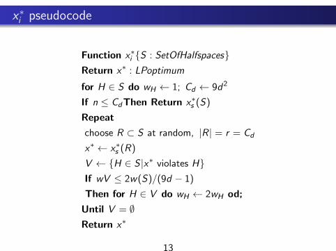
x∗i pseudocode

Function x∗i {S : SetOfHalfspaces}Return x∗ : LPoptimum

for H ∈ S do wH ← 1; Cd ← 9d2

If n ≤ CdThen Return x∗s (S)

Repeat

choose R ⊂ S at random, |R| = r = Cd

x∗ ← x∗s (R)

V ← {H ∈ S |x∗ violates H}If wV ≤ 2w(S)/(9d − 1)

Then for H ∈ V do wH ← 2wH od;

Until V = ∅Return x∗

13

x∗i details

This reweighting technique allows us to choose constraints efficiently.

Choose a random subset R, with probability of selecting a constraintproportional to their weight. Let V be the constraints violated by theoptimum by that subset.

If |V | is low, this subset of inequalities resembles S , so double theweights of these inqualities.

Eventually, the constraints in S∗ has large enough weight that the randomsubset R contains S∗.

Question: Is doubling the weight optimum? Why not triple, or quadruple,the chosen weight? Would this make S∗ ⊆ R faster?

14

The Mixed Algorithm

x∗m is the mixed algorithm, our ”white whale” in terms of complexity.

It is a version of the recursive algorithm x∗r that calls the iterativealgorithm x∗i for its recursive calls.

The motivation for this is to have a time bound with leading termO(d2n) while avoiding the large number of calls to x∗s of the recursivealgorithm.

15

Complexity Analysis

The success of all of these algorithms is based on the following lemma:

Lemma

In the recursive, iterative, and mixed algorithms, if the set V is nonempty,it contains a constraint of S∗.

Draw a picture!

This allows us to be sure that we are making progress with each iterationof the algorithm; elements of S∗ are being reweighted.

16

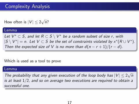
Complexity Analysis

How often is |V | ≤ 2√n?

Lemma

Let V ∗ ⊂ S, and let R ⊂ S \ V ∗ be a random subset of size r , with|S \ V ∗| = n. Let V ⊂ S be the set of constraints violated by x∗(R ∪ V ∗).Then the expected size of V is no more than d(n − r + 1)/(r − d).

Which is used as a tool to prove

Lemma

The probability that any given execution of the loop body has |V | ≤ 2√n

is at least 1/2, and so on average two executions are required to obtain asuccessful one.

17

Complexity Analysis

Theorem

Given an LP problem with b ≥ 0, the iterative algorithm x∗i requires

O(d2 log n) + (d log n)O(d)d/2+O(1)

expected time, as n→∞, where the constant factors do not depend on d.

This is broken down into two steps

The loop body is executed an expected O(d log n) times.

The loop body requires O(dn) + O(d)d/2+O(1). This leading term inn, dn, is from the computation that determines V .

18

Theorem

Complexity Analysis Algorithm x∗m requires

O(d2n) + (d2 log n)O(d)d/2+O(1) + O(d4√n log n)

expected time, as n→∞, where the constant factors do not depend on d.

Idea of proof: At most d + 1 successful (|V | ≤ 2√n) iterations are needed

so that S ⊆ V ∗.

Take away: x∗i (S) does pretty well, but by paying really close attention todetails we can reduce the leading term in n from n log n to n.

19

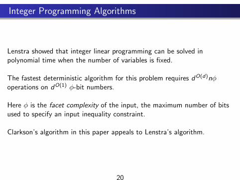
Integer Programming Algorithms

Lenstra showed that integer linear programming can be solved inpolynomial time when the number of variables is fixed.

The fastest deterministic algorithm for this problem requires dO(d)nφoperations on dO(1) φ-bit numbers.

Here φ is the facet complexity of the input, the maximum number of bitsused to specify an input inequality constraint.

Clarkson’s algorithm in this paper appeals to Lenstra’s algorithm.

20

The Integer Case

The basis of the algorithm is a result analogous to Helly’s Theorem.

Theorem

Doignon-Bell-Scarf There is a set S∗ ⊂ S with |S∗| ≤ 2d − 1 and withx∗(S) = x∗(S∗).

In other words, the optimimum of the ILP is determined by a ”small” set.

21

The Integer Case

The ILP algorithms are simply variations on the LP algorithms

Sample sizes using 2d rather than d

Lenstra’s algorithm in the base case

The set S∗ is not necessarily unique. Does Helly’s Theorem guaranteeuniqueness?

22

The Integer Case

We have a similar lemma to the linear case

Lemma

Let V ∗ ⊂ S, and let R ⊂ S \ V ∗ be a random subset of size r > 2d+1,with |S \ V ∗| = n. Let V ⊂ S be the set of constraints violated byx∗(R ∪ V ∗). Then with probability 1/2, |V | ≤ 2d+1n(ln r)/r .

23

The Integer Case

Using this lemma, we have the following modifications for the ILPalgorithms

For the recursive algorithm, put the sample size at 2d√

2n ln n

Use Lenstra’s algorithm with n ≤ 22d+5d

With probability 1/2, the set V will contain no more than√

2n ln nconstraints. Require this for a successful iteration.

For the iterative algorithm, use a sample size of 22d+4(2d + 4), with acorresponding |V | bound of n(ln 2)/2d+3.

24

The Integer Case

Analysis of the ILP mixed algorithm is similar to the LP algorithm

The top level does expected 2d+1n row operations, and generated2d+1 expected subproblems

Each of these subproblems has no more than 2d+1√

2n ln nconstraints.

Each subproblem requires 2d+1 ln n iterations.

Each iteration requires 2d+1√

2n ln n row operations, and a call toLenstra’s algorithm.

25

The Integer Case

These computations yield

Theorem

The ILP algorithm x∗m requires expected

O(2dn + 8d√n ln n ln n)

row operations on O(d3φ)-bit vectors, and

dO(d)φ ln n

expected operations on O(dO(1)φ)-bit numbers, as n→∞, where theconstant factors do not depend on d or φ.

These row operations are just the the evaluation of an inputinequality at a given integral point.Clarkson claims that the integral points can be specified with 7d3φbits.The dO(1)φ-bit numbers comes from Lenstra’s Algorithm.

26

The Clarkson Soup

Clarkson-Type Algorithms

Input

A limit on the number of restrictions necessary to characterize theproblem (Helly’s theorem, Doignon-Bell-Scarf theorem).

A way to solve small problems quickly (Simplex-type algorithm,Lenstra’s algorithm).

A metric of how to verify how similar a subproblem is to the original.How many constraints does the solution to this subproblem violate?

Output

Improved complexity results!

27

The Clarkson Soup

Theme of Clarkson Algorithms:

Choose a boundary for the metric that guarantees forward progresswill be made.I.E. If the number of original inequalities that are violated by therandomly selected constraints is small, then the subproblem contains(mostly) necessary constraints of S .

Choose a sample size so that the probability of this ”success” isgreater than or equal to 1/2.

Do a bunch of random sampling! Outsource small subproblems towhatever the best tool is on the market.

28

K-feasibility Clarkson

Theorem

DeLoera, Iskander, Louveaux If S is an integer program with k feasiblepoints, there is a subproblem consisting of c(d , k) constraints with thesame k-points (and no more).

And so it begins!

We want to use this theorem to establish a Clarkson-type algorithm to findthe best k solutions to S .

Given an arbitrary integer program, we can add the constraintobjectiveS ≥ xk , where xk is the k-th best solution to turn satisfy theconditions for the theorem.

29

Looking Forward

Open Questions and Ideas:

How to check for k-feasibility quickly?Barvinok’s algorithm counts the number of integral points in apolyhedron in polynomial time (in a fixed dimension).

What kind of metric should be used?The number or original constraints violated by the solution to thesubproblem will not work, since we aren’t interested in thepreservation of a single point, but k of them.Also, we don’t have these k points in our hand like we do for Lensta’sand the simplex algorithm!

30

Violator Spaces

One promising generalization of Clarkson-like-algorithms is ViolatorSpaces.

A Violator Space is a pair (H,V ), where H is a finite set and V is amapping 2H → 2H such that

Consistency: G ∩ V (G ) = ∅ holds for all G ⊆ H

Locality: For all F ⊆ G ⊆ H, where G ∩ V (F ) = ∅.

We think of H as the set of constraints that come with a problem, and themap V is the map that, given a subset G returns the constraints in H thatare violated by the optimum over G . (Picture)

31

Basis and Combinatorial Dimension

We say that B ⊆ H is a basis if for all proper subsets F ⊂ B we haveB ∩ V (F ) 6= ∅.

In other words, the smallest (by inclusion) set of constraints that have thesame optimum objective value.

Let (H,V ) be a violator space. The size of a largest basis is called thecombinatorial dimension of (H,V ).

Helly’s Theorem Anybody?!

It turns out that Clarkson’s Algorithm holds for generalized violator spaces.(After proving a non-trivial Sampling Lemma.)

32

Basis and Combinatorial Dimension

We say that B ⊆ H is a basis if for all proper subsets F ⊂ B we haveB ∩ V (F ) 6= ∅.

In other words, the smallest (by inclusion) set of constraints that have thesame optimum objective value.

Let (H,V ) be a violator space. The size of a largest basis is called thecombinatorial dimension of (H,V ).

Helly’s Theorem Anybody?!

It turns out that Clarkson’s Algorithm holds for generalized violator spaces.(After proving a non-trivial Sampling Lemma.)

33

Conclusion

Thanks for listening!

34