on computable beliefs of rational machinestheory.stanford.edu/~megiddo/pdf/compbeli.pdf · on...

On Computable Beliefs of Rational Machines

IBM Research Division, Almaden Research Center, San Jose, California 95120-6099, and School of Mathematical Sciences, Tel Auiv University, Tel Auiv, Israel

Traditional decision theory has assumed that agents have complete, consistent, and readily available beliefs and preferences. Obviously, even if an expert system has complete and consistent beliefs, it cannot have them readily available. More- over, some beliefs about beliefs are not even approximately computable. It is shown that if all players have complete and consistent beliefs, they can compute approximate beliefs about beliefs of any order by considering events arbitrarily close in some well-defined sense to those in question. o 1989 Academic Press. h c .

In traditional decision sciences (see, for example, Luce and Raiffa, 1957) decision makers are usually not assumed to be restricted in their thinking in any way. They have consistent beliefs and preferences which are available throughout the decision making process. The widely ac- cepted Bayesian approach to decision making under uncertainty main- tains that whenever an agent lacks information about the value of a certain variable, s/he still has some "subjective" probability distribution (i.e., beliefs) with respect to such values. The sense of the word "has" in the preceding sentence is that all the probabilities are readily available. Of course, the beliefs are subject to Bayesian updating whenever some new information is received.

There has recently been interest in modeling players as computing machines (see, for example, Binmore, 1987). If the decision maker is a computer program (an "expert system"), rather than an ideal player as in the traditional theory, its beliefs are not readily available. The program may have consistent beliefs which it can only approximate with arbitrary precision. Moreover, for some events with complicated descriptions, the

144 0 8 9 9 - 8 2 5 6 1 8 9 $3 .OO Copyright O 1989 by Academic Press, Inc All rights of reproduction in any form reserved.

COMPUTABLE BELIEFS 145

beliefs may be determined by the basic beliefs but the program cannot even approximate them. It should be noted that in this paper we do not deal with the question of computational complexity at all but rather with the more basic notion of computability. Thus, we are interested here in what expert systems can do in principle and not necessarily in practice.

It is useful to consider beliefs as computable and noncomputable real numbers. A real number a is said to be computable if there exists a computer program A such that, given any rational E > 0, A outputs a rational number a'(&) such that la'(&) - a1 < E . In this sense the program A "knows" the real number a . However, the program can only tell us approximations to a . We believe that a "rational" program should have consistent beliefs in this asymptotic sense, namely, its exact beliefs should be consistent even though the program can only work with approximate beliefs.

Game theory is concerned with situations where more than one decision maker is involved. Players must reason about one another's behavior. In a game of incomplete information, players do not know exactly who the other players are; i.e., they do not know exactly what the other players know about other players. However, Bayesian players have beliefs (in the form of probability distributions) about other players. The foundations for a theory of games with incomplete information played by Bayesian players were given in Harsanyi (1967-1968) (see also Mertens and Zamir, 1985). However, the questions of computability have not been addressed in this context.

In this paper players assume the form of programs residing in computers. We are concerned with the issue of beliefs of programs about other programs and their beliefs. Beliefs about the state of "nature" (as well as beliefs about beliefs about the state of nature, and so on) are suppressed for simplicity of presentation. In other words, states of the world (or "possible worlds") correspond here to combinations of beliefs of players about players. Our discussion here should be considered an extension to the foundations of games with incomplete information played by Bayesian players. Beliefs about beliefs have also been considered by philosophers, mathematicians, and computer scientists. Some references on beliefs can be found in Gaifman (1986), Fagin et al. (1988), Fagin and Halpern (1988), and Konolige (1986).

For the benefit of readers who have not been exposed to the issues of beliefs, we first demonstrate the complications involved in beliefs of players about each other. To simplify the discussion consider henceforth only

146 NIMROD MEGIDDO

2-person games. The extension to any finite number of players is straight- forward.

Suppose none of the players knows exactly who hislher opponent is. For example, suppose none of the players knows whether hislher opponent is a male or a female. However, each player has some belief about the sex of hislher opponent. Let Pi (i = 1, 2) denote the probability with which player i believes hislher opponent is a male. Suppose playerj = 3 - i does not know the precise value of Pi. Thus, slhe considers Pi to be a random variable with some probability distribution F)". Here the superscript ( I ) indicates that this is a belief of level 1. Similarly, player i has a probability distribution F!" with respect to Pj which slhe views as a random variable.

If the players are not restricted in any way then F:" and F)" may already be quite complicated mathematical objects. Note that, in general, the player may be concerned not only with the question of whether the opponent is a male or a female but also with the question of what the opponent believes about the sex of the player hidherself. In principle, each player should have a probability measure on the space of possible opponents. In particular, this space must have a measurable structure relevant to the game. Thus, this structure should reflect not only the sex of the opponent but also the opponent's beliefs about the first player's sex, the beliefs of the second player about the beliefs of the first player about the sex of the second player, and so on. In general, this already raises the need to consider infinite spaces of possible opponents. More specifically, already at the first level player 1, say, must characterize possible opponents not just according to being M (male) or F (female) but also according to types (M, P2) or (F, P2) where P2 (which may be any number between 0 and 1) is the probability which player 2 ascribes to the event that player 1 is a male. Of course, the space of possible opponents must be considered together with a measurable structure.

At the next level, player i does not know what F,!" is, so slhe has some probability distribution ~ 1 ' ) with respect to it. (The superscript (2) indicates a second level of beliefs.) This is a distribution on a class of possible probability distributions of a single random variable. In general, the com- plication of the possible distributions grows quickly with the level of belief. Special care must be given to the problem of measurability. We sometimes talk about levels of events which are the objects of belief. Essentially, the level of an event is the number of times we include a reference to a player in the definition of the event.

We consider below the restricted case where players are identified with finite programs. The set of all possible programs is of course enumerable. This implies severe restrictions on the type of beliefs of players about each other.


Every program has a finite size, yet it reacts to an infinite number of possible inputs. In other words, the behavior of the program in an infinite number of situations is described (implicitly) using finite space. A similar observation applies to the "beliefs" of the program about an infinite number of events. Since the program is finite, it cannot have all its beliefs readily available. Thus it may have to compute some of its beliefs during the decision making process. Of course, the computation is invoked by some signal from the outside, and there are infinitely many possible sig- nals.

The players in our model are programs residing in computers. Recall that we restrict attention to games with two players. Denote by M I , M 2 , . . . the sequence of all possible programs. These programs do not have to exist in the physical sense of the word. They are merely strings of characters. It is easy to construct a one-to-one mapping from programs to natural numbers. Godel constructed such a mapping (for a different pur- pose), so it is quite common to talk about the "Godel number" of a program (or, equivalently, a Turing machine). The details of the mapping are not relevant. However, the important property is that there exists an effective procedure for translating numbers into programs and vice versa.

In our model there are two computers C , , C2, In the beginning these computers are empty (like the "empty shells" in Aumann, 1985). They are then loaded with programs X 1 , X2, respectively. The symbols X I , X2 should be interpreted as random variables whose values are names of programs, or Godel numbers. The latter interpretation is appealing since it makes X I and X2 random variables in the usual sense. Note that we allow for X 1 = X2 since there is no limit on the number of copies of the same program which may be involved in a game.

We do not impose any restriction on the "thinking power" of our players beyond the fact that they are finite programs. We will always assume they are sufficiently smart to compute whatever is needed and computable. Thus, we are aiming at a definition of a class S of those programs which qualify as "smart." In particular, smart programs have complete beliefs about their opponents. If the class S is finite then questions about computability become trivial, so we assume S is infinite. Note that for every program there are infinitely many programs that are equiva- lent to it in the sense that they react in the same way to any input.

The measurable space underlying our discussion is therefore as follows. The points of the space are pairs ( M i , M j ) of programs where Mi and M J are members of a certain subset S of the set of all possible programs. Since the space is enumerable there is no problem in assuming that all the subsets of S x S are measurable. Each program in S has well-defined

148 NIMROD MEGIDDO

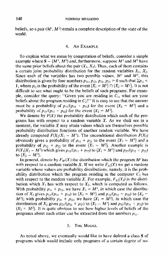
beliefs, so a pair ( M i , M j ) entails a complete description of the state of the world.

To explain what we mean by computation of beliefs, consider a simple example where S = { M I , M 2 ) and, furthermore, suppose M 1 and M 2 have the same prior beliefs about the pair ( X I , X2). Thus, each of them contains a certain joint probability distribution for the random variables X I , X2. Since each of the variables has two possible values, MI and M 2 , this distribution is given by four numbers pl l , p12, p21, p22 2 0 such that 2pi j = 1, where pi, is the probability of the event { X I = M i ) n {X2 = M j ) . It is not difficult to see what ought to be the beliefs of such programs. For example, consider the query: "Given you are residing in C I , what are your beliefs about the program residing in C2?" It is easy to see that the answer must be a probability of p I I I ( p ~ ~ + p12) for the event {X2 = M I ) and a probability of pI2I (pI I + pi2) for the event {X2 = M2).

We denote by F ( X ) the probability distribution which each of the programs has with respect to a random variable X. As we shall see in a moment, the variable X may attain values which are themselves possible probability distribution functions of another random variable. We have already computed F(X21X1 = M I ) . The unconditional distribution F(X2) obviously gives a probability of p l l + pzl to the event {X2 = M I ) and a probability of p12 + pz2 to the event {X2 = M2) . Another example is F ( X , ( X ~ = M ~ ) which gives p12/(p12 + p22) to { X I = M I ) and p d ( p 1 2 + ~ 2 2 )

to {X* = M 2 ) . In general, denote by FMc(X) the distribution which the program M i has

with respect to a random variable X . If we write Fx,(X) we get a random variable whose values are probability distributions, namely, it is the probability distribution which the program residing in the computer C 1 has with respect to the random variable X . For example, Fx,(X2) is the distribution which X I has with respect to X2, which is computed as follows. With probability pl l + p12, we have X I = M I , in which case the distribution of X2 gives pl l l (pl + pI2) to {X2 = M I ) and p121(p12 + pZ2) to {X2 = M2); with probability p21 + p22, we have { X I = M2) , in which case the distribution of X2 gives p21/(p21 + p22) to {X2 = M I ) and p22/(p21 + pZ2) to {X2 = M2) . It is quite obvious to see how higher levels of beliefs of the programs about each other can be extracted from the numbers pi j .

As noted above, we eventually would like to have defined a class S of programs which would include only programs of a certain degree of so-


phistication. These programs would be considered "rational players." The set S would be countable, and we expect it to be infinite.

Our main assumption is that rational players have consistent beliefs. Thus, we assume the following:

A l . Each of the programs in S contains an implicit description of a probability distribution over the "states of the world" (or "possible worlds"), i.e., a joint probability distribution of the random variables XI, X2, signifying the programs residing in the computers C 1 , C 2 .

The implicit presence of a distribution is considered one of the axioms that would characterize programs in the class S. This distribution is an inherent part of the program. It reflects the program's prior probabilities before it is informed of the computer in which it resides. For any program M k E S, denote by pkj the probability which M k ascribes to the event {XI =

M i ) fl {X2 = M i ) . This probability may be viewed as a function of two variables, i, j.

In traditional game theory it is informally assumed to be common knowledge among the players that they are all rational. Accordingly, we assume:

A2. Each program in S ascribes probability zero to any event in which any of the computers C1, C2 stores a program which is not in S.

We do not assume that programs in S can decide whether a given program belongs to the class S.

The objects of belief are events. Recall that the events are precisely the subsets of S x S. Such a subset E represents all instances in which ( X I , X2) E E. However, events are usually described without specifying the sets E directly. In order for a program to "understand" what the event is, there must be an effective procedure which tells for each pair (i, j) whether, say, ( M i , M j ) E E. In such a case we say that the event E is "computable." Obviously there cannot exist more than No computable events.

When an event is described verbally, we can attach to the description a "level number" as follows. First, direct descriptions of the set E will be considered of level 1. On the other hand, a description in the form of a sentence such as " X I ascribes probability greater than 50% to the event that X2 believes with probability greater than 90% that XI = MI7" is to be considered of level 3 . Essentially, descriptions of level v + 1 are stated in terms of beliefs of players about events with descriptions of level less than or equal to v. Note that the level numbers are associated with descriptions of events rather than the events themselves. An event may have descriptions of different levels.

It is trivial to see that the prior distributions { p & ) determine the beliefs

150 NIMROD MEGIDDO

of the programs with respect to any event. Obviously, for every S1, s2 c s,

The latter may constitute an infinite series, convergent, of course. By cardinality arguments, not all the beliefs are computable.

An interesting question is the relation between the description of an event and the computability of its probability. Consider the following example. Denote by E an even in which player 1, say, believes with probability greater than .rro that a certain event E' with a description of level v has occurred. Let pi denote the probability which M k ascribes to {XI = M i } , and let .rri = pi(E'IXI = Mi); i.e., .rri is the conditional probability which Mi ascribes to the event E', given that XI = Mi. Let S1 denote the set of all indices i such that .rri > .rro. Then, obviously,

The quantities pi and .rri are determined by the ps's but there may not exist programs which compute their exact values.

We prefer not to restrict the probabilities ps to be rational numbers. However, since our players are finite programs, we must assume the probabilities are computable. One can distinguish two approaches to computation of beliefs of programs, namely, exact and approximate computation. However, there is a difficulty with the exact computation approach. We might insist that the p$'s be rational numbers but that does not imply that numbers of the form Ej p&pJh,, which are typically involved in the computation of beliefs, will also be rational. It seems unjustified to require that the probabilities of all events be rational numbers, so we adopt the approximate computation approach, which means that the program computes its beliefs with any prescribed precision.

More formally, we assume that given i, j and a rational E > 0, the program M k computes a nonnegative rational number p;(~) such that

Thus the exact belief pkj is the limit (as E tends to zero) of the approximate beliefs pfj(&) which M k computes given the prescribed precision. We of course assume that xi, jpfj = 1. A stronger assumption, namely, 2;. jp; = 1, is reasonable yet not necessary.


In this section we present some elementary facts about computable numbers.

DEFINITION 6.1. A real number a is said to be computable if there is a program A such that, given any rational number E > 0, A computes a rational number 6 = h(e) such that

PROPOSITION 6.2. The computable real numbers constitute a jield.

Proof. The theme in what follows is that the quality of the required approximation can be computed in advance. First note that if a is computable then so is -a. Suppose there exist programs which compute rational E-approximations 6 ( ~ ) and 6 ( ~ ) for a and b , respectively, for any rational e > 0. Thus 16(&) - a1 < E and Ib(&) - bl < E . To approximate a + b, consider the estimate

It implies that a rational &-approximation for a + b can be computed by adding up ~12-approximations of a and b. To approximate ab, consider the estimate

As 6 tends to zero, this computable upper bound tends to zero. Thus, an &-approximation of a + b can be computed by adding up 46) + 6(6), where 6 = l ln and n is the first integer such that

Suppose a f 0. To approximate a-I, assume without loss of generality that for any E , 6(e) f 0 and consider the estimate

For 6 sufficiently small, since a f 0 and 6(6) tends to a , we have

NIMROD MEGIDDO

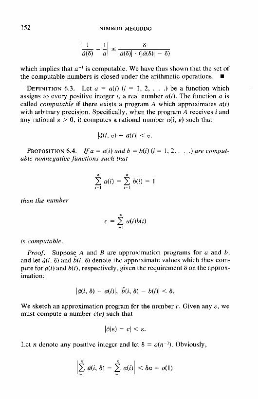
which implies that a-' is computable. We have thus shown tha ~t the set of the computable numbers is closed under the arithmetic operations. rn

DEFINITION 6.3. Let a = a(i) ( i = 1, 2, . . .) be a function which assigns to every positive integer i , a real number a(i). The function a is called computable if there exists a program A which approximates a(i) with arbitrary precision. Specifically, when the program A receives i and any rational E > 0, it computes a rational number i ( i , E ) such that

PROPOSITION 6.4. Zfa = a(i) and b = b(i) ( i = 1 , 2 , . . .) are computable nonnegative functions such that

then the number

is computable.

Proof. Suppose A and B are approximation programs for a and 6, and let n(i, 6) and b(i, 6 ) denote the approximate values which they compute for a(i) and b(i), respectively, given the requirement 6 on the approximation:

We sketch an approximation program for the number c. Given any E, we must compute a number C ( E ) such that

Let n denote any positive integer and let 6 = o(nP1). Obviously,

COMPUTABLE BELIEFS

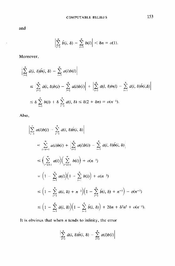
and

Moreover,

Also.

It is obvious that when n tends to infinity, the error

154 NIMROD MEGIDDO

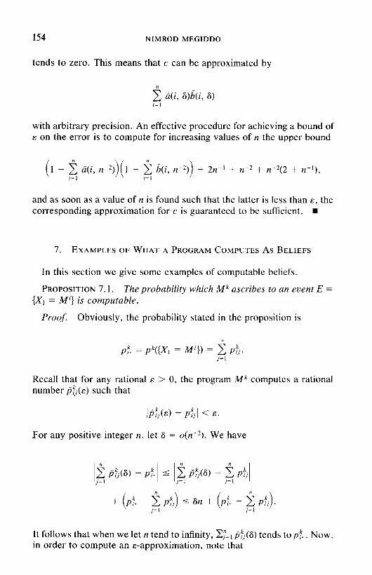
tends to zero. This means that c can be approximated by

with arbitrary precision. An effective procedure for achieving a bound of F on the error is to compute for increasing values of n the upper bound

and as soon as a value of n is found such that the latter is less than E , the corresponding approximation for c is guaranteed to be sufficient.

In this section we give some examples of computable beliefs.

PROPOSITION 7.1. The probability which M k ascribes to an event E =

{ X I = M i ) is computable.

Proof. Obviously, the probability stated in the proposition is

Recall that for any rational E > 0, the program M k computes a rational number B$(E) such that

For any positive integer n , let 6 = o(n-'). We have

It follows that when we let n tend to infinity, B;.(6) tends to pf . . Now, in order to compute an &-approximation, note that

COMPUTABLE BELIEFS

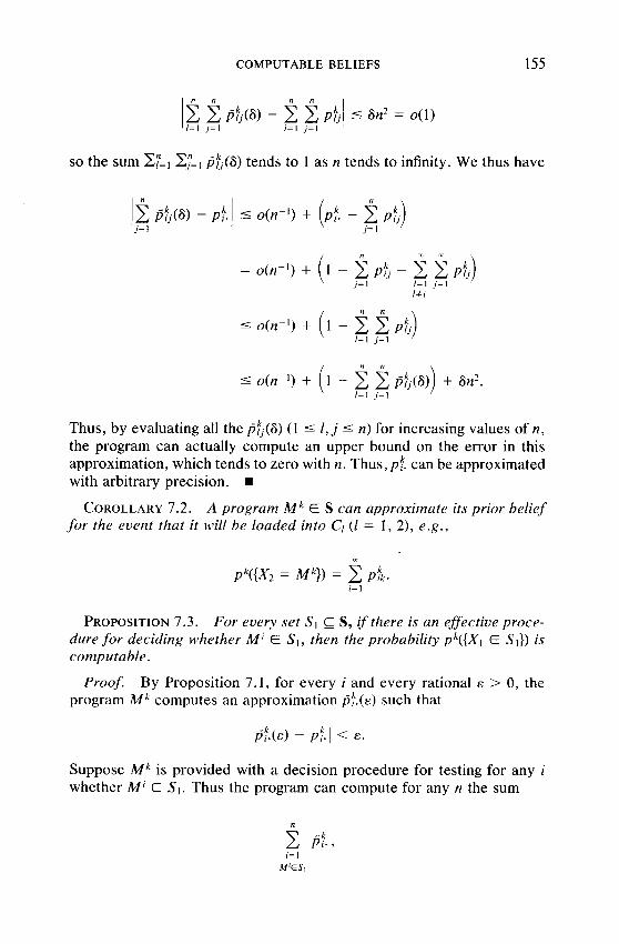
so the sum X;"=, xy=l d h ( 6 ) tends to 1 as n tends to infinity. We thus have

Thus, by evaluating all the sf;.(^) (1 5 I , j 5 n ) for increasing values of n , the program can actually compute an upper bound on the error in this approximation, which tends to zero with n . Thus, pf . can be approximated with arbitrary precision. w

COROLLARY 7.2. A program M k E S can approximate its prior belief for the event that it will be loaded into CI ( I = 1, 2), e.g.,

PROPOSITION 7.3. For every set S 1 S, i f there is an effective procedure for deciding whether M i E S l , then the probability pk({XI E S1}) is computable.

Proof. By Proposition 7.1, for every i and every rational E > 0, the program M h computes an approximation pl.(c) such that

Suppose M k is provided with a decision procedure for testing for any i whether M i E S 1 . Thus the program can compute for any n the sum

156 NIMROD MEGIDDO

and also estimate the difference between the latter and the exact probability. It is easy to see how this implies that the exact probability is computable.

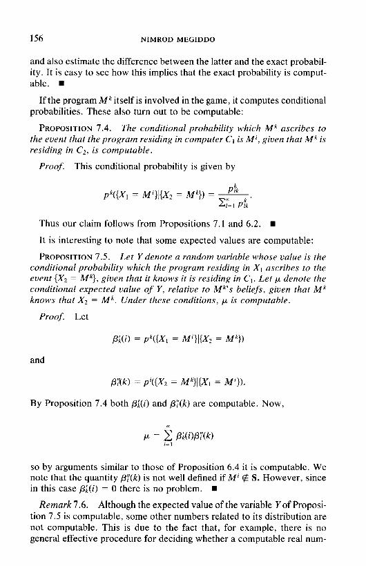
If the program M k itself is involved in the game, it computes conditional probabilities. These also turn out to be computable:

PROPOSITION 7.4. The conditional probability which M k ascribes to the event that the program residing in computer C 1 is M i , given that M k is residing in C2, is computable.

Proof. This conditional probability is given by

Thus our claim follows from Propositions 7.1 and 6.2.

It is interesting to note that some expected values are computable:

PROPOSITION 7.5. Let Y denote a random variable whose value is the conditional probability which the program residing in X I ascribes to the event {X2 = M k } , given that it knows it is residing in C 1 . Let p denote the conditional expected value of Y , relative to M k ' s beliefs, given that M k knows that X2 = M k . Under these conditions, p is computable.

Proof. Let

and

By Proposition 7.4 both P;(i) and P:!(k) are computable. Now,

so by arguments similar to those of Proposition 6.4 it is computable. We note that the quantity p:!(k) is not well defined if M i @ S. However, since in this case P;(i) = 0 there is no problem.

Remark 7.6. Although the expected value of the variable Y of Proposi- tion 7.5 is computable, some other numbers related to its distribution are not computable. This is due to the fact that, for example, there is no general effective procedure for deciding whether a computable real num-


ber a is greater than 1. We can compute s-approximations h(s) of a for any rational s > 0. The case a f 1 is decidable since, if we let s = lln for n =

1 ,2 , . . . , when we reach E < 31a - 1 1 , we observe that I~i(s) - 1 I > E and we then know that a > 1 if and only if h(s) > 1. On the other hand, if a = 1 we may never be able to conclude anything. In fact, there does not exist a general program which can decide, given the description of a program which computes a number a (in the asymptotic sense, with no input), whether a = 1. The proof of this claim is standard and proceeds as follows. Suppose, to the contrary, there exists such a program. Then there exists a program that decides for any program x and any input y whether the number x(y) computed by x in the asymptotic sense, given the input number y, is 1. Furthermore, there exists a program z which computes the number z(x) = 1 given the input x if x(x) f 1, and z(x) = 0 otherwise. It turns out that if z(z) = 1 then z(z) # 1 and if z(z) # 1 then z(z) = 1.

The difficulty pointed out in Remark 7.6 is interesting in its own right. In the traditional theory, when a person wants to find out what hislher subjective probabilityp(E) is for some event, slhe tries to compare p(E) in a binary search fashion with numbers such as 0.5, 0.75, 0.675, and so on, so as to get a good approximation. However, a program can compute approximations but cannot in general perform a single comparison.

Note that it is still possible to perform comparisons in an approximate sense as follows.

PROPOSITION 7.7. If a and b are computable then there exists a program which recognizes for any given rational s > 0 either that a 5 b + E

or that a 2 b - E.

Proof. Let c = b - a and suppose C is a program which computes for any rational s > 0 a rational number E(E) such that If(&) - cl < s . Obvi- ously, if C(s) 2 0 then c > -E, and if E(E) 5 0 then c < F . .

Remark 7.8. Despite the positive tone of Proposition 7.7, there is still a difficulty in computing probabilities as in the following example. Let ak denote the conditional probability (given that X2 = Mk) which M k ascribes to the event that X I ascribes probability of at least 90% to the event that X2 = Mk. The conditional probability

is computable. Let Sk denote the set of indices i such that P:l(k) r 0.9. Then

158 NIMROD MEGIDDO

However, we do not have an effective procedure for deciding whether i E Sk. SO, it seems that a k cannot in general be approximated with an arbitrarily small error.

In this section we present some facts about the computability of the probability distribution of certain random variables.

DEFINITION 8.1. Consider a discrete random variable Y which attains values yi with respective probabilities pi 2 0 (i = 1, 2, . . .). Thus, x:=, pi = 1. We say that Y is computable if there exists a program A that computes &-approximations pi(&) and Yi(&) of pi and yi, respectively, for any i and any rational E > 0.

Denote

S(t) = {i: yi 5 t).

The cumulative distribution function (c.d.f.) of Y is given by

We now consider the problem of approximating the c.d.f. of a computable random variable. For any rational 6 > 0 and any positive integer n , denote

and

Si(6, t) = {i: Ei(6) 5 t - 6, 1 5 i 5 n}.

Let

and

COMPUTABLE BELIEFS

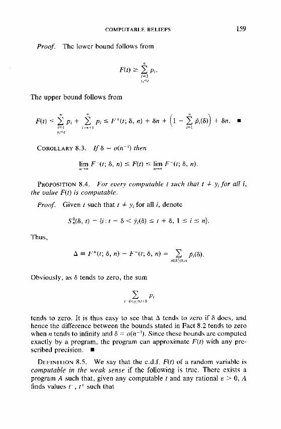
Proof. The lower bound follows from

n

F(t) 2 C Pi. i= l

The upper bound follows from

COROLLARY 8.3. If 6 = o(nPl ) then

lim F - ( t ; 6 , n ) 5 F(t) 5 lim F + ( t ; 6 , n ) . r n m n-m

PROPOSITION 8.4. For every computable t such that t # yi for all i , the value F( t ) is computable.

Proof. Given t such that t # yi for all i , denote

~ f ( 6 , t ) = {i: t - 6 < Yi(6) 5 t + 6 , 1 5 i 5 n}.

Thus,

Obviously, as 6 tends to zero, the sum

tends to zero. It is thus easy to see that A tends to zero if 6 does, and hence the difference between the bounds stated in Fact 8.2 tends to zero when n tends to infinity and 6 = o(nP1) . Since these bounds are computed exactly by a program, the program can approximate F( t ) with any prescribed precision.

DEFINITION 8.5. We say that the c.d.f. F(t) of a random variable is computable in the weak sense if the following is true. There exists a program A such that, given any computable t and any rational E > 0, A finds values t - , t+ such that

160 NIMROD MEGIDDO

and values ~ ( t - , s) and ~ ( t + , E ) such that

and

PROPOSITION 8.6. If Y is a computable random variable then its c.d.f. is computable in the weak sense.

Proof. Consider the computation of t- and ~ ( t - , E ) ; the computation of t+ and ~ ( t + , E ) is analogous. Since t is computable, the program can compute a sequence {t j ) of distinct rational numbers which converges to t from below. For any n let 6 = 6(n) > 0 be smaller than half the minimum distance between any ti f tj such that i , j 5 n. Thus the intervals (ti - 6 , ti + 6) ( i = 1 , . . . , n) are disjoint. It follows that

n n

2 (F+(t;; 6, n) - FP( t i ; 6 , n)) 5 2 pi(6) 5 1 + 6n. i= 1 i= I

This means that the minimum

min ( F f ( t i ; 6, n ) - FP(t i ; 6, n)) I s i s n

tends to zero as n tends to infinity. By choosing t to be a minimizer ti (for sufficiently large n) , we get an &-approximation for F(tP) for a value t- arbitrarily close to t .

COROLLARY 8.7. If Y is a computable random variable, then there exists a program A such that for every computable number y and every rational E > 0, A computes an interval I of length 111 < E , which contains y, and an &-approximation to the probability that Y is in I .

Remark 8.8. If {I,) is a family of intervals containing y, such that II,) < E , then for any random variable Y and any probability measure p,

Thus, the &-approximations claimed in Corollary 8.7 converge to the


probability of { Y = y) . Nevertheless, the program cannot compute E-approximations to the latter with a prescribed E.

Remark 8.9. As noted above, the beliefs of programs with respect to certain random variables may be determined by some consistency re- quirements even though the programs cannot compute them. Thus we may denote by pk({Y = y} ) the probability ascribed by M h to the event { Y = y ) whenever this value is determined by probabilities ascribed by M h o some other events. We have seen examples of such cases where ph( {Y = y} ) is the sum of a well-defined infinite series. The conclusion of Corollary 8.7 suggests that we might relax the definition of computability of a random variable as follows. Let us say that a random variable Y is pseudo-computable for M k if the probability distribution ascribed to Y by M k is well defined and discrete and has the following property. Given any computable y and rational F > 0, M k computes an interval I , 111 < E , which contains y , and an &-approximation to the probability pk({Y E I ) ) . Unfor- tunately, it seems that this notion is yet too restrictive. To clarify this point, suppose Y is pseudo-computable for every M k and let y be any computable number. Denote by Z the probability ascribed by Xi (i.e., the program residing in Ci) to the event { Y = y}. Here Z is not even pseudo- computable since we must replace not only values z of Z by small intervals but also values y of Y by such intervals. We propose below a weaker notion of computability which seems more fit.

We first introduce some notation for discussing more general computable beliefs. Let E be any computable event. For any interval I (which may consist of a single point t ) denote by E [ I ; il the event in which the probability ascribed by Xi to the event E lies in the interval I . Inductively, let

E [ I , , . . . , I,; i l , . . . , ill = {pxl(EIIl , . . . , 1,-I ; i l , . . . , i l - l ] ) € I,}.

- - . .l& f ( x l , . . . , x , ) = l i m . . . lim f ( x , , . . . , x , )

x,-0 x.+O XI-0 x.-0

then we denote the common value of these limits by

Lim f ( x , , . . . , x n ) . I,. ..., x.+O

162 NIMROD MEGIDDO

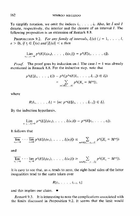
To simplify notation, we omit the indices i l , . . . , il. Also, let f and denote, respectively, the interior and the closure of an interval I. The following proposition is an extension of Remark 8.8.

PROPOSITION 9.2. For any family of intervals, I ~ ( E ) ( j = 1, . . . , 1 , E > 0) , i f t j E ( ( E ) and ll j(~)I < E then

Proof. The proof goes by induction on 1. The case 1 = 1 was already mentioned in Remark 8.8. For the inductive step, note that

where

RII1, . . . , I,] = { m : pm(EII1,

By the induction hypothesis,

Lim pm(E[ l l ( rd , . . . , 4(&1)1) E l I , . . . ,RI+O

It follows that

and

It is easy to see that, as E / tends to zero, the right-hand sides of the latter inequalities tend to the sums taken over

and this implies our claim.

Remark 9.3. It is interesting to note the complications associated with the limits discussed in Proposition 9.2. It seems that the limit would


behave more regularly if we replaced the general families of intervals Ij(&) (a family for each j , satisfying tj E 4 ( ~ ) and JI j (~)I < E ) by sequences of the form 4(&) = (t j - 8 , tj = 8) . However, this simplification implies a limit in the usual sense ("simultaneous") only if 1 < 2. More specifically, first recall that for 1 = 1 we always have

since

Moreover, if { 1 1 ( ~ 1 ) } is a nested family of intervals, then for every k, the function

decreases monotonically to pk(E[ t l ] ) as tends to 0. Now, consider the case 1 = 2. We know that

where

For any fixed 12, let tend to zero, and consider the varying set RIZ1, 12]. Obviously, in this process every m enters this set at most once and leaves it at most once. The contribution of m to p k ( E I I I ( ~ J , 12(g2)1) is pk({Xi2 = Mm}) and the sum of all these values is of course bounded. Thus, this contribution tends to zero as m tends to infinity. It follows that, as E I

tends to zero, the size of the jumps in the value of pk(E[I1(eI ) , I2(c2)1) tends to zero. This means that the limit exists. However, monotonicity is not guaranteed since there can be infinitely many values of m entering and leaving the set RII1, 12] in the limit process, during which I2 is fixed, and this may happen for infinitely many intervals 12. Since monotonicity is not guaranteed, it may happen that in the case 1 = 2, a limit in the usual sense will not exist.

Proposition 9.2 provides the justification for an approximate computation of pk(E[t l , . . . , t,]) in a sense defined below. We first consider the case I = 1.

164 NIMROD MEGIDDO

PROPOSITION 9.4. There exists a program A which does the following. I t receives a program Mk, a computable event E, an index i , and rational numbers t and E > 0. I t then computes an interval I such that t E I and 111 < E, and an E-approximation to the probability pk(EII; i]).

Proof. First, note that

Consider intervals of the form I(6) = (t - 26, t + 26). Denote by pm(E, 6) the 6-approximation computed by M m for pm(E). Let U(6) denote the set of m's such that

Obviously, if m E U(6) then pm(E) E I(6). Let W(6) denote the set of m's such that either

Similarly, if m E W(6) then pm(E) $! I(6). The remaining values of m are those for which either

Denote the set of these m's by V(6). We claim that for every m, there exists 6" = 6*(m) such that for all 6 < 6*, m f$ V(6). For ifpm(E) = t then m E U(6) and ifpm(E) # t then for all 6 sufficiently small m E W(6). Now, for every n


These estimates suggest how to effectively choose n and 6 so as to compute the approximations as required. Specifically, if 6 = o(npl) the difference between the lower and upper bounds on pk(EII; i]) tends to zero as n tends to infinity. Note that both these bounds can be computed exactly. .

We now consider the general case.

PROPOSITION 9.5. There exists a program A which does the following. I t receives a program Mk, a computable event E, indices il, . . . , il, rational numbers tl, . . . , tl, and E > 0. I t then computes open intervals 11, . . . , 4 such that t, E Ij and lIjl < E ( j = I , . . . , I), and an E-

approximation to the probability

pk(EIIl, . . . , Ill) = pk(EII1, . . . , 11; il, . . . , ill).

Proof. We sketch a program which recurses on the value of 1. The case I = 1 was proven in Proposition 9.4. Suppose 1 > 1 and let the inputs Mk, E, ij, tj ( j = 1, . . . , I), and E be given. Recall from the proof of Proposition 9.2 that

where

R[Zl, . . . , I)] = {m: pm(E[Z,, . . . , 11-I]) € I!}

Our program works by recursing to problems of approximating pm (E[ZI, . . . , 11-1]) for m = 1, . . . , n, where n is determined by the program. The complete algorithm therefore computes approximations for pmj (EII1, . . . , I,]} for mj = 1, . . . , nj (where nj is determined by the program) f o r j = 1, . . . , 1 - 1; the intervals Ij turn out to be the same for all values of mj, depending on j. We compute intervals of the form

Actually, the value of is determined with respect to 61, the value of alp2 is determined with respect to and so on. Thus we actually prove the following:

Claim. There exists a program that computes positive rationals 61, . . . , 6l (where 61 < E), positive integers n l , . . . , nl, intervals Ij as defined above, and approximations as follows:

166 NIMROD MEGIDDO

(i) a 6j+l-approximation for pm~+l({X4 = Mrn,)) (mj = 1, . . . , nj),

(ii) a Gj+l-approximation for prn~+l(EII1, . . . , 4]),

where

To prove the claim, suppose we have established the existence of a program which does all the above for the values 1, . . . , j - 1, and consider the case of the value j. Note that only part (ii) of the claim must be proven. We rely on estimates similar to those made in the proof of Proposition 9.4. First, note that if mj E U[61, . . . , 6,] then prn~(EIII, . . . , I,-]]) E I,. Now, let W[61, . . . , denote the set of values of mj such that either

It follows that if mj E W[61, . . . , 6,l thenpm~(EII1, . . . , 4 4 . The remaining values of mj are those for which either

We denote the set of these values of mj by V[6,, . . . , a,]. Given a set of values 61, . . . , for every value of mj, there exists 6; = 6j*(mj; 81, . . . , i3,-1) such that for all 6, < a*,

Now, for every ni we have

COMPUTABLE BELIEFS

and

(where U = U[al, . . . , aj] and V = V[6,, . . . , aj]). These estimates suggest how to effectively choose nj and 6, so as to compute the approximations as required. Specifically, given the requirement aj+ l , we run over values of nj, taking 6, = o(njl). For every aj we recurse and find the approximations and 6's from smaller problems. We then observe the difference between the upper bound and the lower bound derived above. When the latter becomes less than the given aj+,, an approximation as required in (ii) has been found. .

Remark 9.6. It is clear that a stronger result can be proven as follows. Instead of the rational numbers t , , . . . , t , in Proposition 9.5, we could use sets T I , . . . , TI which are computable in some obviously defined sense. For every j, the interval I, would then be interpreted as a Sj-neighborhood of the set T, .

As pointed out earlier, beliefs about computable events are themselves computable. On the other hand, there exist noncomputable events. Among the noncomputable events, we are especially interested in events defined in terms of beliefs about beliefs (and so on) about computable events. The above results indicate that these can be approximated in a natural well-defined sense. A class E of such events is defined as follows. Recall that the sample space (or the space of "states of the world" or "possible worlds") consists of combinations of programs. Thus, we consider a pair of random variables ( X I , Xz) , specifying the programs residing in the two computers which play the game.

We start with the set Eo of computable events. Recall that a subset E of the sample space is called a computable event if there exists a program A which decides for any point x of the space whether x E E. The program A may be considered the description of the event E. It was shown in Propo- sition 7.3 that the probability ascribed by Mk to a computable event is a computable real number. The set of computable events is of course closed under finite union and complementation. Since every subset of the sample

168 NIMROD MEGIDDO

space is a countable union of computable events (namely, singleton sets), it follows by a cardinality argument that there exist noncomputable events which are themselves countable unions of computable ones.

Next, we define a set El as follows. A basic event E' E El is a set of points defined by an inequality of the form

(where E E Eo) which reads: "The probability ascribed to the event E by the program residing in the computer Ci is at least T." The set El is the algebra spanned by the basic events E' (by finite unions and complementation~). We could define E l to be larger by allowing E' to be defined by more general predicates than the inequality given above, but we prefer, for simplicity, not to do so.

As indicated above, events in El are in general not computable. More- over, the probability which a program must ascribe (in order to be consistent) to an event of the type E' may be noncomputable. However, as pointed out in Proposition 9.5, the program can approximate its belief with respect to some event E "close" to E' (for example, E = {pxl(E) 2

7 j ) where 7 j is arbitrarily close to r ) . Inductively, Ej+l is the algebra spanned by events of the form pXl(E) 2 T where E E Ej. Finally, E =

U,"= E, . It is easy to see that every event E E E can be represented by some

computable events, some logical connectives, and some numerical parameters T I , . . . , r,. The sense of the approximate computation is that, given any E > 0, the program computes an event E which is close to E in the sense that the numerical parameters are changed by amounts up to E .

Furthermore, it also computes an &-approximation to the belief with respect to E. Replacing E by E can be easily justified in practice. Note that the computable events involved in the definitions of E and E are the same. Only the numerical parameters which signify probabilities are different. It seems that in every practical situation there exists an E > 0 such that changes in probabilities within E do not really matter.

Since a computer program is necessarily limited in what it can do, there must be some freedom in defining a class of rational programs. It is expected that different classes of programs could serve as candidates. We have considered two properties A1 and A2 of what we see as candidates. Specifically, in a candidate set S each member has a joint probability distribution with respect to the identities of the other players, ascribing probability zero to the event that any player is not in S.


In view of the results proven in this paper, we can say that if a class S has these properties then there exists a class S* as follows. For every member M of S, there exists a member M * of S* which "emulates" M and is also capable of computing its beliefs with respect to events in E in the approximate sense discussed above. This is true because we have proven the existence of a program for carrying out these computations so this program can be "added" to each member of S. Thus, we might add a third requirement which would say that only classes of the form S* qualify as rational. Our results indicate that this third requirement is not too restrictive. To narrow the set of candidate classes even further, one would have to introduce more axioms. Our proposal should be considered a first step away from the classical abstract assumption that all players are rational and that this fact is common knowledge. We have not considered here situations where some players are allowed to be "irrational." Such situations could be difficult for programs to handle since sometimes a "rational" program Mi might ascribe a positive probability to an event where another program Mj does not halt when it attempts to calculate its beliefs. In such a case, the "rational" program would have to compute its belief about whether another program halts in a certain computation.

AUMANN, R. J . (1985). Correlated Equilibrium As an Expression of Bayesian Rationality. Institute of Mathematics, Jerusalem: The Hebrew University.

BINMORE, K. G. (1987). Remodeled Rational Players. London School of Economics. FAGIN, R., AND HALPERN, J. Y. (1988). "Reasoning about Knowledge and Probability," in

Proc. 2nd Conf. on Theoretical Aspects of Reasoning about Knowledge (M. Y . Vardi, Ed.), pp. 227-293. Los Altos, CA: Kaufmann.

FAGIN, R., HALPERN, J. Y., AND MEGIDDO, N. (1988). "Logic for Reasoning about Proba- bilities," in Proc. 3rd IEEE Symp. on Logic in Computer Science, pp. 277-291. Los Angeles, CA: IEEE.

GAIFMAN, H. (1986). "A Theory of Higher Order Probabilities," in Reasoning about Knowledge ( J . Y . Halpern, Ed.). Los Altos, CA: Kaufrnann.

HARSANYI, J. C. (1967-1968). "Games with Incomplete Information Played by Bayesian Players, I, 11, 111," Manage. Sci. 14.

KONOLIGE, K. (1986). A Deduction Model of Belief. London: Pitman. LUCE, R. D., AND RAIFFA, H. (1957). Games and Decisions: Introduction and Critical

Survey. New York: Wiley.

MEGIDDO, N. (1986). Remarks on Bounded Rationality, Research Report RJ 5270. San Jose, CA: IBM Alrnaden Research Center.

MERTENS, J.-F., AND ZAMIR, S. (1985). "Formulation of Bayesian Analysis for Games with Incomplete Information," Znt. J . Game Theory 14, 1-29.

on computable beliefs of rational machinestheory.stanford.edu/~megiddo/pdf/compbeli.pdf · on...

Documents