on convergence to sle6 ii: discrete approximations and

J Stat Phys (2010) 141: 391–408DOI 10.1007/s10955-010-0053-2

On Convergence to SLE6 II: Discrete Approximationsand Extraction of Cardy’s Formula for General Domains

I. Binder · L. Chayes · H.K. Lei

Received: 28 April 2010 / Accepted: 20 August 2010 / Published online: 8 September 2010© The Author(s) 2010. This article is published with open access at Springerlink.com

Abstract We show how to extract Cardy’s Formula for a general class of domains giventhe requisite interior analyticity statement. This is accomplished by a careful study of theinterplay between discretization schemes and extraction of limiting boundary values. Of par-ticular importance to the companion work (Binder et al. in J. Stat. Phys., 2010) we establishthese results for slit domains and for the critical percolation models introduced in Chayesand Lei (Rev. Math. Phys. 19:511–565, 2007).

Keywords Universality · Conformal invariance · Percolation · Cardy’s formula

1 Introduction

In this note we wish to establish the validity of Cardy’s Formula for crossing probabilities ofcertain 2D critical percolation models in a general (finite) domain � ⊂ C (i.e., an open sim-ply connected subset of C). In this introduction we will not be overly concerned with modelspecifics, as the key point of this work is to clarify certain notions concerning discretizationand extraction of appropriate boundary values. While these issues have been addressed tovarious extents in e.g., [4–6, 14, 15, 17], and may seem quite self-evident—at least for nice(i.e., Jordan) domains, a complete and unified treatment for general domains appears to beabsent. Moreover, aside from æsthetic appeal, the generality that appears here is certainlyneeded for the approach of proving convergence to SLE6 outlined in [16] (see also [17])and carried out in [3]. Our efforts will culminate in the establishment of Theorem 5.8 andCorollary 5.11 (which is stated in [3] as Lemma 2.6).

I. BinderDepartment of Mathematics, University of Toronto, Toronto, Ontario, Canadae-mail: [email protected]

L. Chayes · H.K. Lei (�)Department of Mathematics, UCLA, Los Angeles, CA, USAe-mail: [email protected]

L. Chayese-mail: [email protected]

mailto:[email protected]



392 I. Binder et al.

Since it is our intention that this note be self-contained, let us first review themethodology—introduced in [15] and adapted to the models in [7] (see also [3], Sect. 4.1)—by which Cardy’s Formula can be extracted. At the level of the continuum we are interestedin a domain � ⊂ C which is a conformal triangle with boundary components {A, B, C} andmarked prime ends (boundary points) {a, b, c}—all in counterclockwise order—which rep-resent the intersection of neighboring components. At the level of the lattice, at spacing ε,we consider an approximate domain �ε , in which the percolation process occurs and whichtends—in some sense—to � as ε → 0. At the ε-scale, the competing (dual) percolativeforces will be denoted by “yellow” and “blue”.

Let z be an interior point (e.g., a vertex) in �ε . We define the discrete crossing probabilityfunction uB

ε (z) to be probability that there is a blue path connecting A and B, separating z

from C , with similar definitions for vBε (z) and wB

ε (z) along with yellow versions of thesefunctions. For these objects, standard arguments show that subsequential limits exist; twoseminal ingredients are required: First, they converge to harmonic functions with a particularconjugacy relation between them in the interior and second they satisfy certain (“obvious”)boundary values. With these ingredients in hand it can be shown that the limiting functionsare the so called Carleson–Cardy functions. E.g.,

limε→0

uYε = u,

and similarly for the v’s and w’s where, e.g., according to [2], the functions u,v,w are suchthat

F := u + e2πi/3v + e−2πi/3w

is the unique conformal map from � to the equilateral triangle formed by the vertices 1,e±2πi/3. This is equivalent to Cardy’s Formula.

We carry out the above scheme in its entirety for a general class of domains and theirdiscrete approximations which is suitable for our uses in [3], Lemma 2.6/Corollary 5.11.

Remark The appropriate discrete conjugacy relations for the uε, vε and wε have only beenestablished for the 2D triangular site models in [15] and the extension introduced in [7].However, since the RSW estimates are purportedly universal and actually hold for any rea-sonable critical 2D percolation model, in principle we always have limiting functions u,v,w

with some boundary values. Hence most of the content of the present work should apply.However, certain provisos and clarifications will be required; see Remark 5.6.

In the ensuing arguments we will have occasion to make use of the uniformization mapϕ : D → � (where D denotes the unit disk) provided by the Riemann Mapping Theorem.Here we will take ϕ to be normalized so that ϕ(0) = z0 ∈ � for some fixed point z0 wellin the interior of � and ϕ′(0) > 0. We will also identify points on ∂D with boundary primeends of ∂�, via the Prime End Theorem. We refer the reader to e.g., [13] for such issues.Finally, the reader may wish to keep in mind that the reason for addressing most of theissues herein is for application to the case where the curves/slits under consideration arepercolation interfaces/explorer paths; for discussions on this topic we refer the reader to [3].

2 The Carathéodory Minimum

We start by reviewing a standard notion of domain convergence, namely, Carathéodory con-vergence, mainly to phrase it in terms of more elementary conditions which are more conve-

On Convergence to SLE6 II: Discrete Approximations and Extraction 393

nient for our purposes. The reader can find similar conditions/discussions in e.g., Sect. 1.4of [13].

Our general situation concerns a sequence of domains (�n) which converge in somesense to the limiting � along with functions (un, vn,wn) converging to a harmonic triple(u, v,w) satisfying the appropriate conjugacy relations. As a minimal starting point let usconsider the following pointwise (geo)metric conditions for domain convergence:

(iI) If z ∈ �, then z ∈ �n for all n sufficiently large.(iII) If zn ∈ �c

n, then all subsequential limits of (zn) must lie in �c .(e) For all z ∈ �c (including, especially ∂�) there exists some sequence znk

∈ �cnk

suchthat znk

→ z.

Conditions (iI) and (iII) ensure that limiting values of u, v and w in (the interior of)� can be retrieved and are defined by values of un inside �n whereas condition (e) impliesthat �n’s don’t converge to a domain strictly larger than �, so that the boundary values ofu on ∂� might actually correspond to (the limit of) boundary values of un on �n. Indeed,these preliminary conditions turn out to be equivalent to Carathéodory convergence (seee.g., [10]; although in our context we will actually not have occasion to use convergence ofthe relevant uniformization maps). More precisely, first we have the following result, whoseproof is elementary (and we include for completeness):

Proposition 2.1 Consider domains �n,� ⊂ C all containing some point z0. Then the fol-lowing are equivalent:

1. If K is compact and K ⊂ �, then K ⊂ �n for all but finitely many �n.2. (iI) For all z ∈ �, z ∈ �n for all but finitely many �n.

(iII) If zn ∈ �cn, then all subsequential limits of (zn) must lie in �c .

3. If z ∈ �, and δ < d(z, ∂�), then Bδ(z) ⊂ �n, for all but finitely many �n.

Proof (1) ⇒ (2) To see (iI) suppose z ∈ � and d(z, ∂�) > δ, then Bδ(z) ⊂ � and is com-pact and hence we have Bδ(z) ⊂ �n for all n sufficiently large and hence z ∈ �n for all n

sufficiently large; conversely, To see (iII), suppose zn → z with zn ∈ �cn and suppose towards

a contradiction that z ∈ �. Then again arguing as before, Bδ(z) ⊂ �n for n sufficiently large,but then zn ∈ Bδ(z) also for n even larger, which implies that these zn ∈ �n, a contradiction.

(2) ⇒ (3) Again suppose d(z, ∂�) > δ so that Bδ(z) ⊂ �. If it is not the case thatBδ(z) ⊂ �n for n sufficiently large, then we can find a sequence zn ∈ Bδ(z) ∩ �c

n. SinceBδ(z) is compact, there exists a subsequential limit point znk

→ z∗, but then by (iII), z∗ /∈ �,contradicting Bδ(z) ⊂ �.

(3) ⇒ (1) Let K ⊂ � be compact. We can cover K by K ⊂ ⋃x∈K Bδx (x), with δx <

d(x, ∂�). By the assumed compactness, there is a finite subcover K ⊂ ⋃k

i=1 Bδxi(xi). By (3),

for 1 ≤ i ≤ k, there exists Ni such that Bδxi(xi) ⊂ �n for all n ≥ Ni , and hence it is the case

that K ⊂ �m for all m > max{N1,N2, . . . ,Nk}. �

Now the notion of kernel convergence requires, in addition (specifically to condition (1)in the above proposition) that � is the largest (simply connected) domain satisfying theabove conditions. The addition of condition (e) indeed corresponds to maximality; argu-ments similar to those just presented easily lead to the following (whose proof is elementaryand is also included for completeness):

Proposition 2.2 The conditions (iI), (iII), (e) are equivalent to �n converging to � in thesense of kernel convergence.


Proof In light of the above discussion, it is sufficient to show that the condition (e) is equiv-alent to the maximality condition on � required by kernel convergence.

⇒ Suppose � is not maximal and hence � � �′ where �′ satisfies (iI) and (iII). It mustbe the case then there is a point z ∈ ∂� ∩ �′. By condition (e) there exists znk

→ z withznk

∈ �cnk

, but condition (iII) for �′ implies that z ∈ (�′)c , a contradiction.⇐ Conversely, suppose � is maximal and assume towards a contradiction that � does

not satisfy (e), so that there exists some point z ∈ �c and some δ > 0 such that Bδ(z) ⊂ �n

for all n sufficiently large. By the maximality of �, it must be the case that Bη(z) ⊂ � forany η < δ, which implies in particular that z ∈ �, a contradiction. �

It is noted that in the present setting of bounded, simply connected domains, kernel con-vergence is, by the theorem of Carathéodory, equivalent to convergence uniformly on com-pact sets of the corresponding uniformization maps (see e.g., [10], Theorem 3.1). The latternotion is known as Carathéodory convergence and we will use this terminology throughout.

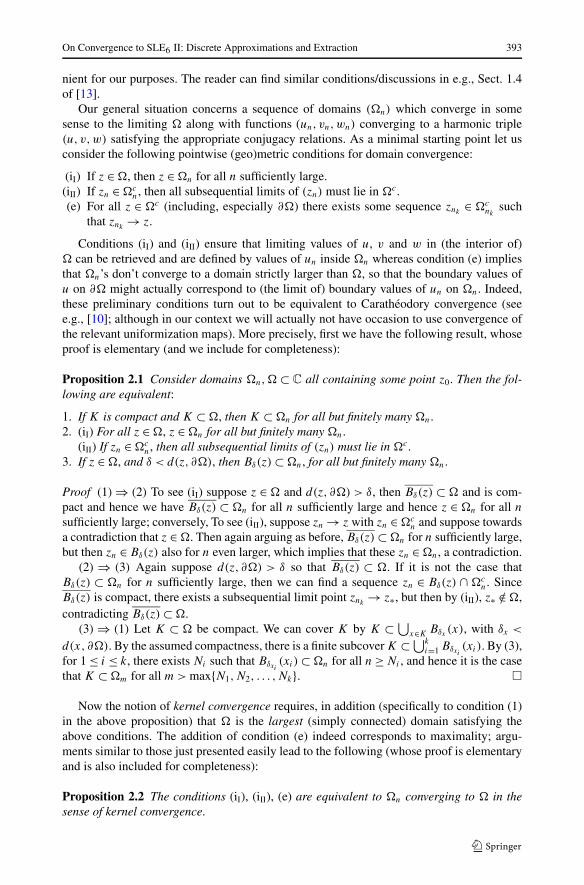
As is perhaps already clear, Carathéodory convergence alone is insufficient for our pur-poses: Since the functions u,v,w must acquire prescribed boundary values on separatepieces of ∂�, it is manifest that (some notion of) separate convergence of the correspondingpieces of the boundary in ∂�n will be required. Special attention is needed for the cases ofdomains with slits—which are of seminal importance when we consider the problem of con-vergence to SLEκ . The situation is in fact rather subtle: Note that in both Fig. 1 and Fig. 3,we have that �ε Carathéodory converges to �, but whereas the situation in Fig. 1 disruptsestablishment of the proper boundary value, the situation in Fig. 3 is perfectly acceptable(see Remarks 3.2 and 4.3).

3 Interior Approximations

We will begin by considering the interior approximations, where �ε ⊂ � for all ε. Forearlier considerations along these lines, see [9] and [11]. Here, the crucial advantage is thatall the �ε’s can be viewed under a single uniformization map; this allows for relativelysimple resolutions of various concerns of a geometric/topological nature. Moreover, thisappears to be the simplest setting for the purposes of establishing Cardy’s Formula in a fixed(static) domain, i.e., where � is fixed for once and for all and we are free to generated �ε inany fashion. (See especially Example 3.3 below.) In particular, for circumstances where thefixed domain problem is all that is of interest, the reader is invited to skip Sect. 4 altogether.We start with:

Definition 3.1 (Interior Approximations) We call (�•ε) an interior approximation to � if:

(I) The domains �•ε consist of one or more (graph) connected components (the latter

case is an artificial effect of the lattice spacing being not fine enough). Each component isbounded by a closed polygonal path, and the union of all such polygonal paths we identifyas the boundary ∂�•

ε . In particular, ∂�•ε consists exclusively of polygonal edges each of

which is a portion of the border of an element in (�•ε)

c .(II) The boundary ∂�•

ε is divided disjoint segments, denoted by Aε, Bε, . . . in (rough)correspondence with the (finitely many) boundary components A, B, . . . of the actual do-main �. In case �ε is a single component, these are joined at vertices aε, bε, . . . corre-sponding to the appropriate marked prime ends. In the multi-component case, if necessary,a similar procedure may be implemented, implying the possible existence of several aε’s etc.


When required, the aε, bε, . . . , etc., will be the one corresponding to the “principal” compo-nent of �ε , namely, the component which contains the point z0, which, we recall, served tonormalize the uniformization map. Here it is tacitly assumed that ε is small enough so thatthis component has a representative of each type.

Further, we require the following:

(i) It is always the case that �•ε ∪ ∂�•

ε ⊂ �. That is, �•ε is in fact a strictly inner approxima-

tion.

This property ensures that indeed all of �ε can be viewed under the (single) conformalmap ϕ : D → � in the ensuing arguments.

(ii) Each z ∈ � lies in �•ε for all ε sufficiently small.

It can be seen that conditions (i) and (ii) imply that for any z ∈ ∂A, there exists somesequence zε → z with zε ∈ Aε , and similarly for B, etc.

(iii) Given any sequence (zε) with zε ∈ Aε for all ε, any subsequential limit must lie in A.Moreover, this must be true in the stronger sense that for any subsequential limitϕ−1(zεn) → ζ ∈ ∂D then ζ ∈ ϕ−1(A). Similarly for B, etc.

In particular, any subsequential limit of the (aε)’s will converge to a point in a, andsimilarly for b, etc.

Remark 3.2

• To avoid confusion, by the above method, an interior approximation to any slit domain—no matter how smooth the slit—necessarily consist of at least a small cavity of a fewlattice spacings. It is noted that the explorer process itself produces just such a cavity.

• It is easy to check that interior approximations satisfy conditions (iI), (iII), (e).• Condition (iii) is indeed used to ensure that the limiting boundary values are unambiguous

and correspond to the desired result (see Lemma 5.2). A simple scenario where carelessapproximation leads to the wrong boundary value is illustrated in Fig. 1.

• Note that even though for convenience we have assumed in (iii) that zε ∈ Cε and haveused the uniformization map ϕ, what is sufficient is that if zk → z ∈ C , then for all butfinitely many k, zk should be close to Cε , in some appropriate sense. Indeed, we shall haveoccasion to formulate such a definition later, for the statement of Lemma 4.4.

Example 3.3 An example of an interior approximation is what we will call the canonicalapproximation, constructed as follows. To be definitive, consider a tiling problem with fi-nitely many types of tiles. We formally define the scale ε to be the maximum diameter of

Fig. 1 Violation of condition (ii)in Definition 3.1, which wouldlead to incorrect (limiting)boundary values


any tile. As usual, we may regard all of C as having been tiled—“Cε”. The domain �ε isdefined as precisely those tiles in Cε which are entirely (including their boundary) in �.Clearly then this construction satisfies (i); condition (ii) is also satisfied: if z ∈ � is such thatd(z, ∂�) > ε0, then z ∈ �ε for all ε < ε0.

At this stage ∂�ε is just one or more closed polygonal paths. The boundary componenttypes are determined as follows: For the marked points, e.g., a, consider the neighborhoodQδ(a) defined as follows: Let cε denote a sequence of crosscuts of ϕ−1(a) with the propertythat ϕ(cε) contains a δ neighborhood of a with δ/ε → ∞ and δ(ε) → 0; Qδ(a) is then the setbounded by ϕ(cε) and the relevant portion of ∂�. It is clear, for ε small, that “outside” theseneighborhoods, the assignment of boundary component type is unambiguous. Here we say aboundary segment is “outside” Qδ(a) etc., if all tiles (intersecting �) touching the segmentin question lie in the complement of Qδ(a). Indeed, each segment of ∂�ε belongs to a tilethat intersects the boundary. For a fixed element of ∂�ε satisfying the above definition of“outside”, some of the external tile is in � and therefore under ϕ−1, the image of this portionof the tile joins up with ∂D; furthermore, it joins with a unique boundary component imagedue to the size of the obstruction provided by Qδ(a). Finally, inside these neighborhoodsQδ(a), etc., all that must be specified are the points aε , etc., which as discussed above, mayhave multiple designations (due to the possibility of multiple components for �ε). The restof the boundary is then assigned accordingly.

Finally, let us establish (iii):

Claim 3.4 The canonical approximation satisfies (iii).

Proof Let zε ∈ Aε with some subsequential limit z. It is clear that z /∈ � since all z ∈ � area finite distance from the boundary while d(zε, ∂�) ≤ ε by construction. Moreover, z ∈ Asince d(zε, A) is (generally less than ε but certainly) no larger than δ(ε). It remains to showthe stronger statement that any subsequential limit of ϕ−1(zε) is in ϕ−1(A). If ζε = ϕ−1(zε)

converges to the image of a marked (end)point in ϕ−1(A) there is nothing to prove. Thuswe may assume that for any κ , eventually ζε is outside the κ-neighborhood of the marked(end)points, which we temporarily denote by α1, α2 ∈ ϕ−1(A). Now let η < κ be such thatthe η neighborhood of ∂D \ [Bκ(α1) ∪ Bκ(α2)] consist of two disjoint components, onecontaining all of the rest of ϕ−1(A) and the other associated with ϕ−1(∂� \ A). Finallyconsider the neighborhood

Mη := Nη(A) ∩ ϕ[Nη(ϕ−1(A)],

where Nη(·) denotes the Euclidean η neighborhood of (·) in the appropriate relative topol-ogy. Since it is agreed that zε stays outside ϕ(Bκ(α1) ∪ Bκ(α2)) it is clear that, for all ε

sufficiently small, zε ∈ Mη and therefore ζε ∈ Nη(ϕ−1(A)) \ [Bκ(α1) ∪ Bκ(α2)] and not in

the complementary η band described above. It follows that the limit must be in ϕ−1(A). �

4 Sup-Approximations

Unfortunately, for various purposes, e.g., certain proofs of convergence to SLE6, we willneed slightly more generality than the internal approximations as provided in Definition 3.1.Specifically, a situation may arise where we have domains �n (given, e.g., stochastically)which are converging, in some sense, to �. One must then contemplate an ε-approximate


Fig. 2 Masking and intermixing of boundary values

for these �n’s—and hence �—and extract some (diagonal) subsequence. However it soonbecomes clear that interior approximations will in general be insufficient: Explicitly, it maybe the case that (�n)εm is not an interior approximation to �, no matter how small εm is.These circumstances can and will readily occur in the pertinent case of slit domains.

Eventually, we will resolve this problem and indeed obtain such a “diagonal” discretiza-tion statement (see Proposition 5.10) by studying more general discretization schemes whichare commensurate with the nature in which �n converges to �. Here, informally, we willdescribe the two additional properties which are essential in our more general context:

• Actual sup-norm convergence of separate sides of the slits (which in the discrete approx-imations may well be separate curves): This is to prevent the masking of one boundaryvalue by another near the joining of boundaries.

• The well-organization property: This is to prevent confusion of boundary values thatcould be caused by intermingling (crisscrossing) of the two curves approximating theopposite sides of the slit.

Scenarios in violation of these properties are depicted in Fig. 2.

Remark 4.1 If γ1 and γ2 are two curves, then as usual the sup distance between them isgiven as

dist(γ1, γ2) = infϕ1,ϕ2

supt

|γ1(ϕ1(t)) − γ2(ϕ2(t))|.

For certain purposes, it is pertinent to consider weighting the sup-norms of portions of thecurves in accord with the particular crosscut in which the portion resides. We will denote theassociated distance by Dist; see [3], Sect. 3.2 for the definition and discussions. However,our ensuing arguments will not be sensitive as to whether we are using the original sup-normor the weighted version and thus we will continue to use the sup-norm.

Definition 4.2 (Sup-approximations) Suppose ∂� can be further divided (perhaps by othermarked boundary points) with the boundary between these points described by Jordan arcsor, more generally, Löwner curves. We shall label the new points J1, J2, etc., and betweencertain pairs, e.g., Jk & Jk+1 will be a Löwner curve denoted by [Jk, Jk+1]. The marked


prime ends a, b, . . . may serve as an endpoint of (some of) these segments, but it is under-stood that they do not reside inside these arcs.

Some of this curve (often enough all of it) will be part of the boundary ∂�. (On the otherhand, it can be envisioned that a portion of this curve lives in a “swallowed” region and ispart of �c .) At the discrete level, we recall that ∂�ε is automatically a union of closed self-avoiding curves. It will be supposed that �ε has corresponding J ε

1 , J ε2 , . . . and the relevant

portion of the curve between the relevant J -pair converges in sup-norm to the correspondingportions in ∂�—or �c , as the case may be—at rate η(ε).

We assume that all of this transpires in such a way that the following property, which wecall well-organized, holds: For any curve of interest [J ε

k , J εk+1], pick points p and p′ on this

arc. Consider δ-neighborhoods around p and p′ and consider the portion of the arc joiningthese neighborhoods (last exit from neighborhood around p to first entrance to neighborhoodaround p′), which we label L . Let P be any path connecting the boundaries of theseneighborhoods to one another in the complement of all of ∂�ε . Then the relevant portionsof ∂Bδ(p), ∂Bδ(p

′), P and L clearly form a Jordan domain, whose interior we denoteby O. Let O′ ⊂ O denote the connected component of P in O \ ∂�ε . Then, ∂O′ ∩ ∂�ε ismonochrome, i.e., it cannot intersect both [J ε

k , J εk+1] and [J ε

, J ε +1] for k �= . While this may

sound overly complicated, what we have in mind is actually a simple topological criterion,c.f., Remark 4.3.

The rest of the domain and boundary is approximated by interior approximation. Thus,for those Jk’s which divide arc-portions of ∂� from “other”, we require commensurability atthe joining points. In particular, in order that the interior approximation be implementable,it is clear that we must require J ε

k ∈ �.

Remark 4.3

• While at first glance it is difficult to imagine that ∂O′ is anything except, say L , whatwe have in mind is when L and a neighboring curve are some approximation to a two-sided slit. A crisscrossing approximation can very well lead to incorrect limiting boundaryvalues—or none at all. The well-organized property does not permit the sides of the ap-proximation to crisscross one another. Alternatively, this is a simple topological criterionwhich can be rephrased as follows: Under the uniformization map (in fact any homeomor-phism onto a Jordan domain would do) the image of each of these J -pieces occupies asingle contiguous piece of the boundary. This sort of monochromicity property is requiredfor well-behaved convergence of relevant boundary conditions which we shall need later.It is clear that this well-organized property is satisfied by the trace of any discrete perco-lation explorer process.

• Sup-approximations satisfy conditions (iI), (iII), (e).• The added difficulty here is that since the approximation is no longer interior, we can no

longer determine the “topological situation” by looking under a single conformal map.E.g., for a point close to the boundary, we can no longer determine which boundary pieceit is “really” close to. This is exemplified by the case of a slit domain: If, say, part ofC is one side of a two-sided slit γ , then points close to γ on one side (correspondingto C ) will have small u value which tends to 0 whereas points close to γ on the otherside (corresponding to say B) will tend to non-trivial boundary values. In the case ofinterior approximation all such ambiguities were resolved by looking under the conformalmap ϕ−1.

• It is worth noting that the important case in point where the boundary consist of an original� with a (Löwner) slit—which might be two sided—falls into the setting under consid-eration. In particular, we will have occasion to consider cases where we have γn → γ in


Fig. 3 A case where the limitingdomains does not contain acomponent present inapproximating domains. Due tofrequent self-touching, such(limiting) domains are in facttypical of SLE6

the sup-norm with γn being discrete explorer paths. In this case to check condition (iII),we observe that if γn → γ in sup-norm and zn ∈ γn and zn → z, then z ∈ γ and hencecertainly in the complement of the domain of interest � \ I(γ ) (i.e., � delete γ togetherwith components “swallowed” by γ ). For an illustration see Fig. 3. These circumstancesmay be readily approximated by a hybrid of sup- and canonical approximations and, as isnot hard to see, satisfy the condition of commensurability.

The main addition is the following lemma which serves the role of condition (iii) inDefinition 3.1 to ensure unambiguous retrieval of boundary values (see Lemma 5.3). Thatis, if w ∈ � is close to C in the “homotopical sense” that any short walk from w whichhits ∂� must hit the C portion of ∂� then w is close to Cn by the same criterion. A precisestatement of this intuitive notion is, unfortunately, much more involved.

Lemma 4.4 (Homotopical Consistency) Consider a domain � with marked boundaryprime ends a, b ∈ ∂�. Let us focus on boundary C with end points a and b which we con-sider to be the bottom of the boundary. (Note that C may consist of Jordan arcs together witharbitrary parts—if double-sided slits are involved, such that not both sides belong to C , thenthe corresponding arc(s) must be connected all the way up to b and/or a). Let us denote thesup-approximation to � by �n and the portion of the boundary approximating C by Cn.

Suppose we have a point w which is more than � away from a and b and δ� away from Cwith � � δ�, such that ϑ = ϕ−1(w) is close to ϕ−1(C). Then there exists η > 0 with η � δ�

such that if dist(Cn, C) < η (here dist denotes e.g., the sup-norm distance where appropriate,and otherwise the Hausdorff distance) then there exists some path P from (some point in)ϕ−1(B�(a)) to (some point in) ϕ−1(B�(b)) (we denote this by ϕ−1(B�(a)) � ϕ−1(B�(b)))such that in the sup-approximation �n, w is in the bottom component of �n\ϕ(P∪B�(a)∪B�(b)) and further, any walk from w in the bottom component which hits ∂�n must hit Cn.

Proof For clarity, we divide the proof into four parts.


Fig. 4 The domain Vn , etc

1. We let η � � � 1 and consider, under the uniformization map, the set

B := D \ [ϕ−1(B�(a)) ∪ ϕ−1(B�(b))].Let us now draw a path P ′ : ∂ϕ−1(B�(a)) � ∂ϕ−1(B�(b)) which defines top and bot-tom components in B with ϑ in the bottom component, and hence also the bottom com-ponent of ϕ(B) \ ϕ(P ′). Further, P := ϕ(P ′) is some finite distance δ � η > 0 awayfrom w. (In essence, δ will now play the role of δ� in the statement of the lemma.)

2. We now look at the domain

Vn = �n \ [B�(a) ∪ B�(b) ∪ P].We claim that for n sufficiently large, all of the above is well-defined: Indeed, P is acompact set in � and hence for n sufficiently large, is contained in �n, by Proposition 2.1.Of course, �n itself may have many components; we are focusing on the principal com-ponent. Even so, with the above setup, Vn may also have many components, e.g., nearthe boundaries of B�(a) and B�(b) (see Fig. 4).

However, we claim that it has the analogue of a top and bottom component: Indeed, itis clear that “large” compact sets in B well away form the boundaries continue to lie inlarge connected components of Vn. More quantitatively, while at the scale �, ∂�n maycreate various components by entering and re-entering B�(a) and B�(b), since Cn andC are η-close (say in the Hausdorff distance), if we shrink these neighborhood balls toscale � − 2η, then such components merge into (the) two principal components, leavingonly η-scale small components in the vicinity of the neighborhood balls.

Finally, we claim that w is in the bottom component of Vn. First, since Bδ(w) mustall be in the same component of Vn, w cannot be in a small η-scale component. Theargument can be finished by any number of means. For example we may choose to re-gard P as two-sided; the component of w is determined by which side of P it may beconnected to. For future reference, let Q′ ⊂ D denote a simple path (staying well awayfrom ∂B) connecting ϑ to P ′ and Q the image of Q′ under ϕ. Then, again, by Propo-sition 2.1, for all n sufficiently large, the entirety of Q is found in �n and the appropriate


component—bottom—for w is determined for once and all. The relevant domains, etc.,are illustrated in Fig. 4.

3. It is clear that w is close to Cn. We further claim that it is not obstructed from Cn by otherportions of ∂�n, as may be the worry when a portion of C is (one side of) a two-sidedslit. We need to divide into a few cases. First if the only portion of C which is close to q isapproximated interiorly, then by an investigation of the situation under the uniformizationmap, it is clear that no obstruction is possible. So now we suppose that w is close to someJordan arc J := [Jk, Jk+1]. If J is one-sided, then there is no problem, since then w

is not close in anyway to any other portion of the boundary except near the endpoints,which we may assume, by shrinking relevant scales if necessary, that w is far away from.

4. We are down to the main issue where J is a two-sided slit, which is being sup-normapproximated by Jn. Since at least one of the end points must be a or b, let us assumewithout loss of generality that Jk = a. We will need to do some refurbishing, startingwith the neighborhood balls around a (and b, if necessary). Let q be a point on Jnear a. It is manifestly the case that q has two images under ϕ−1—which are near ϕ−1(a);consider a crosscut between these two images; the image of this crosscut under ϕ thendefines the relevant neighborhood, which we will denote by e.g., B(a). We note that(i) by construction, B(a) has the property that J enters exactly once and terminatesat a, and (ii) being slightly more careful if necessary to ensure the relevant crosscut iscontained in ϕ−1(B�(a)), we can also ensure that B(a) ⊂ B�(a)). Here we will considerη � dist(a, ∂B(a)), so that in particular, e.g., an ∈ B(a).

Now let us return attention to �n. We will now refurbish P so that it directly joins an tobn and avoids all of ∂�n; we will call the resultant path Pr . We claim that it is possible todraw such a Pr by suitably extending P, under the above stipulations concerning B(a),B(b), and η. Focusing attention on B(a), if this were not possible, then it must have been thecase that a portion of Jn or a portion of ∂�n \ Jn which is approximating the other sideof J , is obstructing. This scenario implies an inner domain inside B(a) surrounding thetip an with boundary e.g., Jn. Since η � dist(a, ∂B(a)), this violates sup-norm η close-ness. (Here it appears that the sup-norm closeness property is crucial. For an illustration seeFig. 5.)

Having achieved all this, it is again clear that the principal component of �n is di-vided into two disjoint Jordan domains. Indeed by the fact that the approximation is well-organized, there are two circuits—both using Pr , passing through an and bn, such that one(which again is the bottom one) contains Cn and the other contains (the principal componentof) �n \ Cn, with no possibility of mixing via crisscrossing. Since Pr is an extension of P,it is clear from the closing argument of (3) that w is in the bottom component and hencemust be closed to Cn without obstruction from any portion of ∂�n \ Cn. �

5 Verification of Boundary Values for u,v,w

We are now in a position to verify boundary values for u,v,w using RSW estimates. Letus begin with a more detailed recapitulation/clarification of how we take the scaling limitof uε, vε,wε (see [15] and [7]). Consider some exhaustion Kn ↗ �, with Kn compact. TheRSW estimates imply equi-continuity, and hence we have u(n)

εk→ u(n) uniformly on Kn and,

at least for the models in [15] and [7],

F (n) := u(n) + e2πi/3v(n) + e−2πi/3w(n)


Fig. 5 Failure to continue P toPr inside B(a)

is analytic there with

u(n) + v(n) + w(n) = const.

We may take (ε(n+1)k ) ⊂ (ε

(n)k ) as a subsequence which implies that

u(n+1)εk

→ u(n+1)

etc., so that F (n+1) is analytic in Kn+1 with values agreeing with the old F (n) in Kn. Thediagonal sequence (u(n)

εn) converges uniformly on compact sets to some u; together with

similar statements for v and w, we obtain that the limiting F is analytic on �. In the sequelfor simplicity we will drop the (n) superscripts and just write e.g., uε → u.

We begin with a lemma which provides us with the RSW technology which is necessaryfor establishing boundary values.

Lemma 5.1 Let � and ϕ be as described. The pre-image of ∂� under ϕ is divided intoa finite number of disjoint (connected) closed arcs the intersection of any adjacent pair ofwhich is the corresponding (pre-image of the) prime end. Then for z ∈ ∂� \ {a, b, c, . . . },we identify z with a single ϕ−1(z) := ζ and similarly identify its corresponding boundarycomponent.

(I) There exists an infinite sequence of (“square”) neighborhoods (S ) centered at z suchthat S ∩� �= ∅ for all and S +1 is strictly contained in S with ∂S containing portionsof the boundary component containing z and

(II) In each S \ S +1, there is a “yellow” circuit and/or a “blue” circuit which separatesz from all other boundary components with probability that is uniformly positive asε → 0 (provided that ε is sufficiently small depending on ). By separation it is meant


that in the pre-image in D, ζ , is separated from all other boundary components alongany path in D whose image under ϕ tends to z.

Finally, for z ∈ {a, b, c, . . . }, a similar statement holds, except for the fact that here therelevant circuits separate z from all other boundary points and boundary components towhich z does not belong.

Proof Let z ∈ ∂� and let ζ = ϕ−1(z) denote its corresponding pre-image. First supposez /∈ {a, b, c, . . . } so that ζ is some finite distance from the corresponding points on ∂D. Thenconsider a sufficiently small crosscut � of D surrounding ζ (a finite distance away from ζ )whose end points on ∂D, denoted α and β , are such that α and β are in the (“interior” ofthe) boundary component of ζ . We also denote by Q the image of the interior of the regionbounded by � and the relevant portion of ∂D; we note that z ∈ ∂Q. Let S0 ⊂ C be a smallsquare centered at z whose intersection with � lies entirely inside Q. Then by construction,∂(S0 ∩�) can contain at most boundary pieces from the boundary component of z. Now thesequence (Sn) will be constructed similarly, with the stipulation that the linear scale of S +1

is reduced by half from that of S .By standard RSW estimates for the percolation problem in all of C, there is a blue and/or

yellow Harris ring inside each annulus S \ S +1 with probability uniformly bounded frombelow for ε sufficiently small. Now consider any path P in D which originates at ζ andends outside ϕ−1(Q) such that the image of the path originates at z. Such a path stays in �

and therefore must intersect the said circuit.Identical arguments hold for z ∈ {a, b, c, . . . } except for the fact that the original crosscut

will now originate and end on two distinct boundary components. �

It is noted that in the presence of a circuit in S \ S +1, the above separation argumentalso applies to points in ∂(Sm ∩ Q) if m ≥ + 1.

Lemma 5.2 (Establishment of Boundary Values for Interior Approximations) Let � and ϕ

be as described. We recall that uBε (z) is the probability at the ε level that there is a blue

crossing from Aε to Bε , separating z from Cε , and let u denote the limiting function. Thenu = 0 on C in the sense that if zk → z ∈ C in such a way that ϕ−1(zk) = ζk → ζ ∈ ϕ−1(C),then limk→∞ u(zk) = 0. Similarly, in the vicinity of the point c, u tends to one. Analogousstatements hold for vB

ε and wBε and for the yellow versions of these functions.

Proof Suppose a yellow Harris circuit has occurred in S \S +1 and let zk → z as described.Then, in the language of the proof of Lemma 5.1, for k sufficiently large zk ∈ Q ∩ Sm forsome m = m(k) tending to ∞ as k → ∞. For ε sufficiently small, it follows from (iii) inDefinition 3.1 that Aε and Bε are disjoint from (Sm ∩ Q ∩ �•

ε) and since �•ε is an inte-

rior approximation, the relevant portion of the circuit evidently joins with ∂Cε to separate∂Sm ∩ Q ∩ �•

ε from c, as for z as discussed near the end of the proof of Lemma 5.1. Thisseparation would preclude the crossing event corresponding to uB

ε (zk) since—as is clear ifwe look on the unit disc via the conformal map ϕ−1—the latter necessitates (two) blue con-nections between the relevant portions of ∂Sm and other boundaries. Now consider k withm(k) very large; then for all ε sufficiently small, the probability of at least one yellow circuitis, uniformly (in ε), close to some p(m) where p(m) → 1 as m → ∞. It therefore followsthat u(zk) ≤ 1 − p(m(k)) → 0 as zk → z. Finally, boundary value of c follows the sameargument: Here the blue Harris ring events accomplish the required connection between Aε

and Bε . Arguments for other functions/boundaries are identical. �


Lemma 5.3 (Establishment of Boundary Values for Sup-approximations) Let � and ϕ beas described. We recall that uB

ε (z) is the probability at the ε level that there is a blue cross-ing from Aε to Bε , separating z from Cε , and let u denote the limiting function. Then u = 0on C in the sense that if zk → z ∈ C in such a way that ϕ−1(zk) = ζk → ζ ∈ ϕ−1(C), thenlimε→0 uB

ε (zk) → 0. Similarly, in the vicinity of the point c, u tends to one. Analogous state-ments hold for vB

ε and wBε .

Proof We recall that we have three boundary pieces A, B, C in counterclockwise order,where we assume without loss of generality that C is on the bottom. We also label therelevant marked prime ends a, b, c, in counterclockwise order, such that e.g., c is oppositeto C . Thus if we draw a path P between aε and bε inside �ε , and zk ∈ �ε is inside theregion formed by P and Cε then to prevent events which contribute to uB

ε , it is sufficientto seal zk off from cε by a yellow Harris ring together with the bottom boundary Cε . This isprecisely the setting of Lemma 4.4 (with w = zk) and so we conclude that for k sufficientlylarge, for ε sufficiently small depending on k, in order to prevent events contributing to uB

ε ,it is indeed sufficient to seal zk off with a yellow Harris ring.

We are now in a position to invoke Lemma 5.1. The proof follows closely as in the lastpart of the proof of Lemma 5.2 except for one difference: For k sufficiently large, zk ∈ Sm forsome m = m(k) which increases as k increases; however, in the case of sup-approximation,it is no longer quite so automatic that arbitrarily small Harris rings will hit the boundaryCε . However, given ε, we have that Cε is at most a distance η(ε) from C , and thus, for fixedε0, there is some M(ε0) such that m(k) ↗ M(ε0) as k → ∞ (and M(ε0) → ∞ as ε0 → 0).So we still have that uniformly for all ε ≤ ε0, Uε(z) ≤ 1 − p(M(ε0)), where p(M(ε0)) asbefore denotes the probability of at least one yellow Harris ring in the annulus S1 \ SM(ε0),and tends to 1 as M(ε0) tends to infinity. �

Remark 5.4 Our arguments in fact show that the function u is continuous up to the boundary:Given any sequence zk → z ∈ C , we have that given any κ > 0, for k sufficiently large,|u(n)

εn(zk)| < κ , uniformly in n, for n sufficiently large (or ε sufficiently small) and hence

u(zk) < κ (c.f., the end of the proof of Theorem 5.5). We have similar statements for v andw on the corresponding boundaries.

To check that F is indeed the appropriate conformal map and thereby uniquely determineit and retrieve Cardy’s Formula, we follow the arguments in [2]. We remark that while thereexists certain literature on discrete complex analysis (see e.g., [11] and [8] and referencestherein) our situation is less straightforward since e.g., none of the functions uN, vN,wN areactually discrete harmonic. Moreover, due to the fact that we are considering general do-mains (versus Jordan domains) and ∂� may not be so well-behaved, to obtain conformalityrequires some extra work. In any case, we will now amalgamate all ingredients to prove thefollowing result:

Theorem 5.5 For the models described in [7] (which includes the triangular site problemstudied in [15]), consider the function F = u + e2πi/3v + e−2πi/3w, where u,v,w are thelimits of uε, vε,wε . Then F is the unique conformal map between � and the equilateraltriangle T with vertices at 1, e2πi/3, e−2πi/3.

Proof We claim that the following seven conditions hold:

1. F is nonconstant and analytic in �,


2. u,v,w (and hence F ) can be continued (continuously) to ∂�,3. u + v + w is a constant,4. u(c) = 1, with similar statements for v and w at a and b,5. u ≡ 0 on C with similar statements for v and w on A and B,6. F ◦ ϕ maps ∂D bijectively onto ∂T,7. (F ◦ ϕ)(D) ∩ (F ◦ ϕ)(∂D) = ∅;

from which the proposition follows immediately. Indeed, from conditions 7 and 6, F ◦ ϕ :D → T is a conformal map (this follows directly from e.g., Theorem 4.3 in [12]). But clearly,conditions 5, 4, 3 imply that F maps � into T, and further, conditions 2 and 1 imply thatF maps � onto T (this follows from e.g., Theorem 4.1 in [12]). Altogether, conformality ofF itself now follows: It is enough to show that F ′ never vanishes, but this follows from thefact that 0 �= (F ◦ ϕ)′(z) = F ′(ϕ(z))ϕ′(z).

We now turn to the task of verifying conditions 1–7. It follows from [7, 15], and [2] thatF is analytic and that u + v + w is constant. On this basis, the real part of F is proportionalto u plus a constant and it is seen from Lemma 5.2 (or Lemma 5.3) that u is not constant,i.e., it is close to 1 near c and close to 0 near C . We have conditions 1 and 3. Conditions 2,4, 5 follow from Lemma 5.2 (or Lemma 5.3) and Remark 5.4.

To demonstrate condition 7, let us write Re(F ) = (3/2)u − 1/2. Then if we show thatu �= 0 in �, then we have demonstrated that F(�) does not intersect F(C). The latter followssince once z ∈ �, we can construct a tube of bounded conformal modulus connecting Ato B going underneath z, and within this tube, by standard percolation arguments whichgo back to [1], we can construct a monochrome path separating z from C . Condition 6follows in a similar spirit: E.g., on the A boundary, if z �= q , but |z − q| � 1, then by theargument of Lemma 5.1, u(z) is close to u(q) (since both can be surrounded by many annuliin which e.g., a blue circuit occurs). Similar arguments for v and w and other boundariesdirectly imply continuity of all functions on all boundaries of �. Moreover, this implies,e.g., u ◦ ϕ−1(A) is continuous on the relevant portion of the circle starting (at ϕ−1(c)) withthe value 1 and ending (at ϕ−1(b)) with the value 0 and thus achieving all values in [0,1].Similarly statements hold for the other functions on the other boundaries. Condition 6 nowfollows directly. �

Remark 5.6 It is worth noting that while using only arguments involving RSW bounds,we have determined that (1) the u,v,w’s can be continued to the boundary and (2) partialboundary values, e.g., u ≡ 0 on C , sufficient determination of boundary values requires addi-tional ingredients. In particular, we also needed that e.g., v + w ≡ 1 on C ; this would followfrom u + v + w ≡ 1 which at present seems only to be derivable from analyticity consider-ations. Duality implies e.g., vB

ε + wYε ≡ 1 on C , but we cannot go any further without color

symmetry as in the site percolation on the triangular lattice case [15] or some (asymptotic)color symmetry restoration as was established for the models in [7].

Definition 5.7 Let us define, as in [3], Cε(�ε, aε, bε, cε, dε) to be the crossing probabilityof the rectangle (�ε, aε, bε, cε, dε) with percolation also taking place at the ε-scale.

Next consider the (unique) conformal map which takes (�,a, b, c, d) to (H,1 −x,1,∞,0), where, clearly, 0 < x < 1 and x = x(�,a, b, c, d). Then we denote byC0(�,a, b, c, d) the function

∫ x

0 (s(1 − s))−2/3 ds∫ 1

0 (s(1 − s))−2/3 ds, (1)

i.e., Cardy’s Formula.


Let us recall/observe that C0(�,a, b, c, d) is equal to e.g., u(d) with d ∈ A (see Sect. 1).We now have

Theorem 5.8 For the models described in [7] with the assumption M(∂�) < 2 (which in-cludes the triangular site problem studied in [15], where the assumption on ∂� is unneces-sary) Cardy’s Formula can be established via an interior or sup-approximation, i.e.,

Cε(�ε, aε, bε, cε, dε) → C0(�,a, b, c, d)

if (�ε) is an interior or sup-approximation to �.

Proof For the site percolation model, this follows from [2, 7, 15], and Theorem 5.5. For themodel described in [7], the interior analyticity statement in sufficient generality is verifiedin [3], Sect. 4.4. �

Finally, let us single out the cases that will be used in the proof of the Main Theoremin [3].

Corollary 5.9 Consider the models described in [7] (which includes the triangular siteproblem studied in [15]) on a bounded domain � with boundary Minkowski dimension lessthan two (if necessary) and two marked boundary points a and c. Suppose we have X

ε[0,t] →

X[0,t] in the Dist norm where Xε[0,t] is the trace of a discrete Exploration Process starting at

a and aiming towards c, stopped at some time t , then

Cε(�ε \ Xε[0,t],X

εt , bε, cε, dε) → C0(� \ X[0,t],Xt , b, c, d).

Further, it is possible to extract a slightly stronger statement which will be used in theproof of the Main Theorem in [3]. For the sake of [3] we will state these results in the Distnorm (c.f., Remark 4.1). For purposes of clarity, we first state a lemma:

Proposition 5.10 Let us denote the type of (slit) domain under consideration by �γ andabbreviate, by abuse of notation, e.g., Cε((�

γ )ε) := Cε(�ε \ γε([0, t]), γε(t), bε, cε, dε) (buthere, γ could stand for other boundary pieces as detailed in Definition 4.2). Then for anysequence γn → γ in the Dist norm and any sequence (εm) converging to zero,

limn,m→∞Cεm

[(�γn)εm

] = C0(�γ ),

regardless of how n and m tend to infinity. Here all approximations are sup-approximations.

Proof From Lemma 5.3 we have that e.g., if γ (n)εm

→ γn is any sup-approximation, thenCεm [(�γn)εm ] → C0(�

γn). The result follows by noting that γ (n)εm

is also a sup-approximationto γ as both m,n → ∞. We emphasize that the reason for such robustness of Lemma 5.3 isbecause the proof is completely insensitive to how γε converges to γ as ε → 0. All that isneeded is that γε is sufficiently close to γ and ε is sufficiently small, which is inevitable if ε

is tending to zero and γε is tending to γ . �

Corollary 5.11 Consider the models described in [7] (which includes the triangular siteproblem studied in [15]) on a bounded domain � with boundary Minkowski dimension lessthan two (if necessary) and two marked boundary points a and c. Consider Ca,c,�, the set


of Löwner curves which begin at a, are aiming towards c but have not yet entered the �

neighborhood of c for some � > 0. Suppose we have γε → γ e.g., in the Dist norm, then

Cε(�ε \ γε([0, t]), γε(t), bε, cε, dε) → C0(� \ γ ([0, t]), γ (t), b, c, d)

pointwise equicontinuously in the sense that

∀κ > 0, ∀γ ∈ Ca,c,�, ∃δ(γ ) > 0, ∃εγ ,

such that

∀γ ′ ∈ Bδ(γ )(γ ), ∀ε ≤ εγ ,

|Cε(�ε \ γε([0, t]), γε(t), bε, cε, dε)

− Cε(�ε \ γ ′ε([0, t]), γ ′

ε(t), bε, cε, dε)| < κ.

(2)

Here Bδ(γ ) denotes the Dist neighborhood of γ .

Proof This is immediate from Proposition 5.10. Negation of the conclusion in the state-ment means that there exists a sequence γn → γ and εn → 0 such that |Cεn((�

γn)εn) −Cε((�

γ )εn)| > κ > 0 for all εn, which clearly contradicts the fact that both of these objectsconverge to the limit C0(�

γ ). �

Remark 5.12 We remark that (2) holds even if “ε = 0” and thus implies continuity ofCardy’s Formula in the “Dist norm”. However, we note that Lemma 5.3, being merely alimiting statement, would be highly inadequate if one had in mind some uniformity of theconvergence or uniformity of the continuity.

Acknowledgements The authors are grateful to the IPAM institute at UCLA for their hospitality and sup-port during the “Random Shapes Conference” (where this work began). The conference was funded by theNSF under the grant DMS-0439872. I.B. was partially supported by the NSERC under the DISCOVER grant5810-2004-298433. L.C. was supported by the NSF under the grant DMS-0805486. H.K.L was supported bythe NSF under the grant DMS-0805486 and by the Dissertation Year Fellowship Program at UCLA.

The authors would also like to thank Wendelin Werner for useful discussions which took place duringthe Oberwolfach conference Scaling Limits in Models of Statistical Mechanics and which led to the presentapproach.

Open Access This article is distributed under the terms of the Creative Commons Attribution Noncommer-cial License which permits any noncommercial use, distribution, and reproduction in any medium, providedthe original author(s) and source are credited.

References

1. Aizenman, M., Chayes, J.T., Chayes, L., Frohlich, J., Russo, L.: On a sharp transition from area law toperimeter law in a system of random surfaces. Commun. Math. Phys. 92(1), 19–69 (1983)

2. Beffara, V.: Cardy’s formula on the triangular lattice, the easy way. In: Universality and Renormalization.Fields Institute Communications, vol. 50, pp. 39–45. AMS, Providence (2007)

3. Binder, I., Chayes, L., Lei, H.K.: On convergence to SLE6 I: conformal invariance for certain models ofthe bond-triangular type. J. Stat. Phys. (2010). doi:10.1007/s10955-010-0052-3

4. Bollobás, B., Riordan, O.: Percolation. Cambridge University Press, Cambridge (2006)5. Camia, F., Newman, C.M.: Two-dimensional critical percolation: the full scaling limit. Commun. Math.

Phys. 268(1), 1–38 (2006)6. Camia, F., Newman, C.M.: Critical percolation exploration path and SLE6: a proof of convergence.

arXiv:math.PR/0604487 (2006)

http://dx.doi.org/10.1007/s10955-010-0052-3

http://arxiv.org/abs/math.PR/0604487


7. Chayes, L., Lei, H.K.: Cardy’s formula for certain models of the bond-triangular type. Rev. Math. Phys.19, 511–565 (2007)

8. Chelkak, D., Smirnov, S.: Discrete complex analysis on isoradial graphs. arXiv:0810.2188v19. Duffin, R.J.: Potential theory on a rhombic lattice. J. Comb. Theory 5, 258–272 (1968)

10. Duren, P.L.: Univalent Functions. Springer, Berlin (1983)11. Ferrand, J.: Fonctions préharmoniques et fonctions préholomorphes. Bull. Sci. Math. 2 68, 152–180

(1944)12. Lang, S.: Complex Analysis. Springer, Berlin (1999)13. Pommerenke, C.: Boundary Behavior of Conformal Maps. Springer, Berlin (1992)14. Ráth, B.: Conformal invariance of critical percolation on the triangular lattice. Available at:

http://www.math.bme.hu/~rathb/rbperko.pdf15. Smirnov, S.: Critical percolation in the plane: conformal invariance, Cardy’s formula, scaling limits.

C. R. Acad. Sci. Paris Sr. I Math. 333, 239–244 (2001). Also available at http://www.math.kth.se/~stas/papers/percras.ps

16. Smirnov, S.: Towards conformal invariance of 2D lattice models. In: Proceedings of the InternationalCongress of Mathematicians, Madrid, Spain (2006)

17. Werner, W.: Lectures on two-dimensional critical percolation. arXiv:0710.0856

http://arxiv.org/abs/arXiv:0810.2188v1

http://www.math.bme.hu/~rathb/rbperko.pdf

http://www.math.kth.se/~stas/papers/percras.ps

http://www.math.kth.se/~stas/papers/percras.ps

http://arxiv.org/abs/arXiv:0710.0856

on convergence to sle6 ii: discrete approximations and

Documents