on dividend policy... merchant renewables and the valuation of peaking plant in energy-only markets...

www.eprg.group.cam.ac.uk

Merchant renewables and the valuation of peaking plant in energy-only markets EPRG Working Paper 2002

Cambridge Working Paper in Economics 2002

Paul Simshauser Abstract Merchant renewables are a new asset class. With historically high cost structures and low wholesale prices associated with merit order effects, continuity of entry has been reliant on Renewable Portfolio Standards or other policy initiatives such as government-initiated Contracts-for-Differences. But in Australia’s National Electricity Market, sharply falling costs of renewables and volatile wholesale market conditions from coal plant exits has led to a surprising number of merchant intermittent renewable investments. Adding to the merchant renewable fleet are older wind plants whose inaugural long-dated PPAs recently matured. Rolling over PPAs is possible, but not necessarily optimal. In this article, a merchant gas turbine, merchant wind, and an integrated portfolio comprising both plants are valued in the NEM’s South Australian region. Asset valuations reveal surprising results. The modelling sequence shows stand-alone gas turbine valuation metrics suffer from modest levels of missing money, that merchant wind can commit to some level of forward (fixed volume) swap contracts in-spite of intermittent production, but the combined portfolio tightens overall valuation metrics significantly. Above all, the combined portfolio is financially tractable, overcoming the missing money for a gas turbine plant undertaking peaking duties. In a NEM region where intermittent renewable market share exceeds 50%, this suggests the energy-only, real-time gross pool design may yet be deemed suitable vis-à-vis meeting environmental objectives and Resource Adequacy. Keywords Merchant renewables, peaking plant, power plant valuations JEL Classification D61, L94, L11 and Q40

Contact [email protected] Publication January 2020 Financial Support N/A

mailto:[email protected]

Merchant renewables and the valuation of peaking plant in energy-only markets

Paul Simshauser♣♠1

January 2020

Abstract Merchant renewables are a new asset class. With historically high cost structures and low wholesale prices associated with merit order effects, continuity of entry has been reliant on Renewable Portfolio Standards or other policy initiatives such as government-initiated Contracts-for-Differences. But in Australia’s National Electricity Market, sharply falling costs of renewables and volatile wholesale market conditions from coal plant exits has led to a surprising number of merchant intermittent renewable investments. Adding to the merchant renewable fleet are older wind plants whose inaugural long-dated PPAs recently matured. Rolling over PPAs is possible, but not necessarily optimal. In this article, a merchant gas turbine, merchant wind, and an integrated portfolio comprising both plants are valued in the NEM’s South Australian region. Asset valuations reveal surprising results. The modelling sequence shows stand-alone gas turbine valuation metrics suffer from modest levels of missing money, that merchant wind can commit to some level of forward (fixed volume) swap contracts in-spite of intermittent production, but the combined portfolio tightens overall valuation metrics significantly. Above all, the combined portfolio is financially tractable, overcoming the missing money for a gas turbine plant undertaking peaking duties. In a NEM region where intermittent renewable market share exceeds 50%, this suggests the energy-only, real-time gross pool design may yet be deemed suitable vis-à-vis meeting environmental objectives and Resource Adequacy. Keywords: Merchant renewables, peaking plant, power plant valuations. JEL Codes: D61, L94, L11 and Q40.

1. Introduction

Renewable Portfolio Standards and government-initiated Contracts-for-Differences (CfD) have been important policy measures for Variable Renewable Energy (VRE) entry, viz. wind and solar PV. Historically high VRE total average costs meant side-payments were essential for entry continuity. Compounding matters were so-called merit order effects – as more priority dispatched VRE entered, the supply curve shifted to the right placing downward pressure on clearing prices. Merit order effects reinforced requirements for side-payments, with remaining plant profitability adversely affected. Plant undertaking peaking duties, essential for reliability purposes, are thought to be particularly vulnerable (Hach and Spinler, 2016; Höschle et al., 2017; Bublitz et al., 2019; Milstein and Tishler, 2019)2. This called into question whether energy-only markets are able to meet both environmental and Resource Adequacy objectives. In the classic VRE entry case, renewables are placed into Special Purpose Vehicles, project financed and underpinned by long-dated run-of-plant Power Purchase Agreements (PPA) written by investment-grade utilities in response to Renewable Portfolio Standards (~9400MW in Australia’s NEM) or government-initiated CfDs (~1800MW3). Equity invested, usually by infrastructure funds, sought stable running yields over time. This investment model of the ‘non-market facing’ VRE plant will no doubt continue.

♣ Professor of Economics, Griffith Business School, Griffith University. Views expressed in this article are those of the author. ♠ Research Associate, Energy Policy Research Group, University of Cambridge. 1 I am indebted to my friend and colleague Dr Joel Gilmore for his extensive assistance building the Stochastic DCF Valuation model used in this research. 2 It is worth noting that in the NEM, it was baseload plant that were most adversely affected due to higher fixed & sunk costs. 3 Also includes government-initiated Feed-in Tariffs for utility-scale plant.

But sharply falling VRE costs and longer-run business cycle dynamics of merit order effects mean alternate entry models are emerging. In Australia’s National Electricity Market (NEM) a surprising number of VRE plant have entered on a fully merchant basis4 – 18 solar PV projects (~1500 MW) and 5 wind projects (~870 MW) reached financial close during 2017-2019 (Panjkov, 2019). Moreover, at least 10 mature incumbent wind plants (~600MW) have simultaneously found themselves with merchant exposures as inaugural 10-15 year PPAs had run full-term. Furthermore, a rising number of VRE entrants (with PPAs) deliberately oversized entry capacity to acquire residual merchant exposures (~650MW). Consequently, Australia’s NEM is accumulating a surprising amount of merchant VRE capacity. From an investment perspective, merchant VRE is a new asset class. In an energy-only market with a Market Price Cap of AUD $14,700/MWh5 – amongst the highest in the world – it is probably not an investment class for the feint hearted given stochastic output. Rolling-over PPAs with incumbent Retailers is possible but may not be profit maximising.6 Indeed as this research reveals, managing merchant VRE is no more challenging than managing stochastic retail loads. VRE can participate in spot and forward markets while managing risks of ‘high price - low output’ events. Resource Adequacy in energy-only markets is a matter of constant interest to energy economists and policymakers, marked by a growing body of literature (Keay, 2016; Bhagwat et al., 2017; Keppler, 2017; Simshauser, 2018; Billimoria and Poudineh, 2019; Bublitz et al., 2019; Milstein and Tishler, 2019). Yet even with rising VRE, provided reliability criteria has a tight nexus with the Market Price Cap7 there should be no question that investment in energy-only markets will flow under conditions of diminishing supply-side reserves. Imbalances induce a growing number, and intensity of, price spike events which drives investment in new capacity (Simshauser and Gilmore, 2019). The central question is whether plant investments occur in a timely manner rather than in response to a crisis, noting practical political limits exist vis-à-vis the severity and duration of wholesale market price shocks (Besser, Farr, and Tierney 2002; Hogan 2005; Simshauser 2018; Bublitz et al. 2019). The central objective of this article is to analyse the most complex of merchant investment commitments in energy-only markets – a price-taking Open Cycle Gas Turbine (OCGT) plant undertaking peaking duties, and, merchant wind. OCGT investments are challenging because predicting peak prices requires much more information than prediction of baseload prices. By their nature, peaking plant operate only during power system imbalances – extreme weather events, material plant outages or market power events. And because such events are inherently uncertain, peaking plant income streams from spot markets are manifestly random and particularly hazardous (Peluchon, 2003; Bidwell and Henney, 2004; Simshauser, 2008). But markets have a way of navigating uncertainty. Practical evidence from Australia’s NEM is that gas turbines have been delivered on a timely basis through altering vertical business boundaries. Of the 7250MW of gas turbine plant developed between 2000-2019, 5350MW (75%) was via vertically-integrated merchant utilities8. This dominant investment thesis had its underpinning in real options9 as a ‘physical hedge’ against stochastic customer load. As

4 Merchant plant sell their output into the spot market and hedge price risk using short-term forward markets. 5 All financial numbers expressed in AUD unless otherwise specified. AUD $14,700/MWh equates to ~US$10,143/MWh and £7791/MWh (AUD/US ~0.69 and AUD/GBP ~0.53) at the time of writing. 6 When an Independent Power Producer (IPP) negotiates with a large utility, the threat of not entering is used to avoid sub-optimal outcomes. Once a plant is sunk, the IPP loses this credible threat. 7 In theory, from a power system planning perspective the overall objective function is to minimise 𝑉𝑉𝑉𝑉𝑉𝑉𝑉𝑉 𝑥𝑥 𝑈𝑈𝑈𝑈𝑈𝑈 + ∑ 𝑐𝑐(𝑅𝑅)𝑛𝑛

𝑖𝑖=1 | 𝑉𝑉𝑉𝑉𝑉𝑉𝑉𝑉 𝑥𝑥 𝑈𝑈𝑈𝑈𝑈𝑈 + 𝑐𝑐�𝑅𝑅�� = 0, where 𝑉𝑉𝑉𝑉𝑉𝑉𝑉𝑉 is the Value of Lost Load, 𝑈𝑈𝑈𝑈𝑈𝑈 is Unserved Energy, and where 𝑐𝑐(𝑅𝑅) is the cost generation plant, and 𝑐𝑐�𝑅𝑅�� is the cost of peaking plant capacity. Provided these conditions hold, it can be said there is a direct relationship between Reliability and the Market Price Cap. An alternate expression where reliability criteria is based on Loss of Load Expectation is 𝑉𝑉𝑉𝑉𝑉𝑉𝑈𝑈 = 𝐶𝐶𝐶𝐶𝐶𝐶𝑈𝑈/𝑉𝑉𝑉𝑉𝑉𝑉𝑉𝑉, where CONE is the cost of new entry. For an excellent discussion on the relationship between a Market Price Cap and reliability criteria, see (Zachary, Wilson and Dent, 2019). 8 That is, large competitive Retail Supply businesses with generation portfolios, or merchant generators with significantly integrated forward Retail Supply positions. 9 The origins of which can be traced back to (Myers, 1977).

vertical investments, gas turbines evidently overcame the many frictions, imperfections and bounded rationality that characterise forward electricity markets (Roques, Newbery and Nuttall, 2005; Simshauser, Tian and Whish-Wilson, 2015; Newbery, 2016). Merchant VRE presents an alternate investment thesis for gas turbines. Just as OCGTs have more stable valuations when marked against stochastic customer load, more stable values should, in theory, be achievable when marked against market-facing stochastic merchant VRE plant. In the following analysis, OCGT and merchant wind are valued as stand-alone investments, then combined as a merchant portfolio. The rich volatility associated with cyclical and structural energy-only market variations are captured using a diverse array of market conditions – 100 years of stochastic spot price data with 30-minute resolution based on the NEM’s South Australian region, where VRE market share now exceeds 50%. Non-convexities, imperfect plant availability and other important features of gas turbines are incorporated in a Unit Commitment Model which aggregates and transposes 30-minute data into 100 years of annual results. A Stochastic DCF Valuation Model then uses a Monte Carlo sub-sampling process to randomly draw annual results from the Unit Commitment Model to populate each future year of the plant’s useful life. This Monte Carlo sub-sampling process is iterated 500 times to produce a valuation distribution for the various merchant generation assets. Valuation results confirm stand-alone OCGT plant is marginally sub-economic10, and that stand-alone wind in Australia’s NEM can commit to a portfolio of forward Swaps (or 2-way CfDs) in-spite of intermittent production. When integrated, OCGT expected returns exceed entry costs, and the combined portfolio is found to have a materially tighter distribution of net revenues under a very wide range of wholesale market conditions – an important characteristic given capital market requirements. Above all, the combined portfolio seems capable of ‘finding the missing money’. These findings present important implications for policymakers. Modelling suggest when OCGT is integrated with merchant VRE in the NEM, tractable financial results emerge as a function of transaction cost economics.11 By implication, the NEM’s energy-only market appears capable of delivering peaking plant capacity on an economic basis (i.e. Resource Adequacy) with very high levels of VRE (i.e. >50% VRE market share). Whether these results can be generalised to other jurisdictions is contingent on the relative pattern of VRE output and the relationship between Dispatch-Weighted and baseload prices. This article is structured as follows. Section 2 reviews relevant literature. Section 3 outlines model inputs. Section 4 introduces the suite of models and Section 5 presents results. Conclusions follow. 2. Review of Literature

There is enduring interest in the ability of energy-only markets to deliver power system reliability due to adequacy of generation plant returns. Reliability should ideally be broken down into its component parts, viz. Resource Adequacy and System Security12 (Batlle and Pérez-Arriaga, 2008). To be clear, the focus in this article is strictly Resource Adequacy in the context of i). energy-only markets ii). with rising VRE, and iii). and the valuation of gas turbine plant, each of which are reviewed below.

10 At least at this point in the energy market business cycle. 11 On transaction costs and vertical integration in the NEM, see Simshauser, Tian and Whish-Wilson (2015). 12 Resource Adequacy means adequate installed plant capacity relative to expected peak demand and is essentially a long run concept (given entry lags). System Security means the configuration of power system resources dispatched and enabled, and their ability to deal with credible contingencies – and is thus a real-time concept.

2.1 Energy-only markets Resource Adequacy concerns in energy-only markets can be loosely traced back to Von der Fehr and Harbord (1995) who noted indivisibility of capacity, construction lead-times, lumpy entry, investment tenor and policy uncertainty make merchant generation unusually risky investments. Early contributions on peaking plant include (Doorman, 2000; Besser, Farr and Tierney, 2002; Stoft, 2002; de Vries, 2003; Oren, 2003; Peluchon, 2003).13 Bublitz et al., (2019) provide an excellent summary of the rapidly growing literature in the field. Of central concern is the stability of earnings and missing money, a concept formally introduced by Cramton and Stoft (2005, 2006). The central idea behind missing money is net revenues earned in energy-only markets are suboptimal cf. expected returns. Peaking plant are thought to be particularly susceptible given manifestly random revenues in organised energy-only spot markets (Peluchon, 2003; Simshauser, 2008; Bajo-Buenestado, 2017; Keppler, 2017; Milstein and Tishler, 2019). Economic theory and power system modelling has long demonstrated organised spot markets can clear demand reliably and provide suitable investment signals for new capacity (Schweppe et al. 1988). But theory and modelling is based on equilibrium analysis with unlimited market price caps, limited political and regulatory interference, and by deduction – largely equity capital-funded generation plant able to withstand elongated ‘energy market business cycles’ (Simshauser, 2010; Arango and Larsen, 2011; Cepeda and Finon, 2011; Bublitz et al., 2019). Good economic theory often collides with harsh realities of applied corporate finance. In practice, energy-only markets are rarely in equilibrium. Persistent pricing at marginal cost does not result in a stable equilibrium given substantial sunk costs – a problem understood at least as far back as (Hotelling, 1938; Boiteux, 1949; Turvey, 1964). Because merchant generators face rigid debt repayment schedules, theories of organised spot markets suffer from an inadequate treatment of how non-trivial sunk capital costs are financed (Joskow, 2006; Finon, 2008; Caplan, 2012).14 Generator pricing must deviate from strict marginal cost at some point, but given oligopolistic market settings distinguishing between loss-minimising behaviour and an abuse of market power is difficult (Cramton and Stoft, 2005, 2008; Roques, Newbery and Nuttall, 2005; Joskow, 2008; Simshauser, 2008). Further, actions by regulatory authorities and System Operators frequently suppress legitimate price signals (Joskow, 2008; Hogan, 2013; Spees, Newell and Pfeifenberger, 2013; Leautier, 2016)15. Australia’s NEM is also suffering from various forms of political interference (Simshauser, 2019b; Wood, Dundas and Percival, 2019). Risks to timely entry may arise from capital constraints. In the early phases of the global restructuring and deregulation experiment, a vast fleet of merchant plant was project financed on the basis of forecast spot prices and short term forward contracts (Joskow, 2006; Finon, 2008; Simshauser, 2008).16 But recurring damage to merchant generator profit & loss statements, a product of structural oversupply and episodes of missing money, eventually led project banks to tighten risk tolerances and credit metrics (Simshauser, 2010).17

13 See also (Bushnell, 2004; Wen, Wu and Ni, 2004; Neuhoff and De Vries, 2004; Hogan, 2005, 2013; Roques, Newbery and Nuttall, 2005; Cramton and Stoft, 2006; Simshauser, 2008; Finon, 2008; Finon and Pignon, 2008; Joskow, 2008; Spees, Newell and Pfeifenberger, 2013; Cramton, Ockenfels and Stoft, 2013). Entire editions of academic journals have been dedicated to the topic. See for example Utilities Policy Volume 16 (2008) or Economics of Energy & Environmental Policy Volume 2 (2013). 14 Fixed and sunk costs in energy-only markets are, in theory, recovered during price spike events. But participants are unable to optimise the frequency and intensity of price spikes (Cramton and Stoft, 2005). Moreover Market Price Caps are frequently set too low (Batlle and Pérez-Arriaga, 2008; Joskow, 2008; Petitet, Finon and Janssen, 2017; Bublitz et al., 2019; Milstein and Tishler, 2019) in which case a stable financial equilibrium can only be reached if the power system is operating near the edge of collapse (Bidwell and Henney, 2004; Simshauser and Ariyaratnam, 2014). 15 See also (Besser, Farr and Tierney, 2002; de Vries, 2003; Oren, 2003; Wen, Wu and Ni, 2004; Batlle and Pérez-Arriaga, 2008; Finon and Pignon, 2008). 16 This included 230,000MW in the US, 13,000MW in Australia and more than 6000MW of new plant in the UK. See (Joskow, 2006; Finon, 2008; Simshauser, 2010) for details. 17 By 2005, more than 110,000 MW of merchant plant in the US, much of the Australian merchant fleet and various high profile plant in the UK (e.g. Drax) experienced financial distress or bankruptcy (Joskow, 2006; Finon, 2008; Simshauser, 2010).

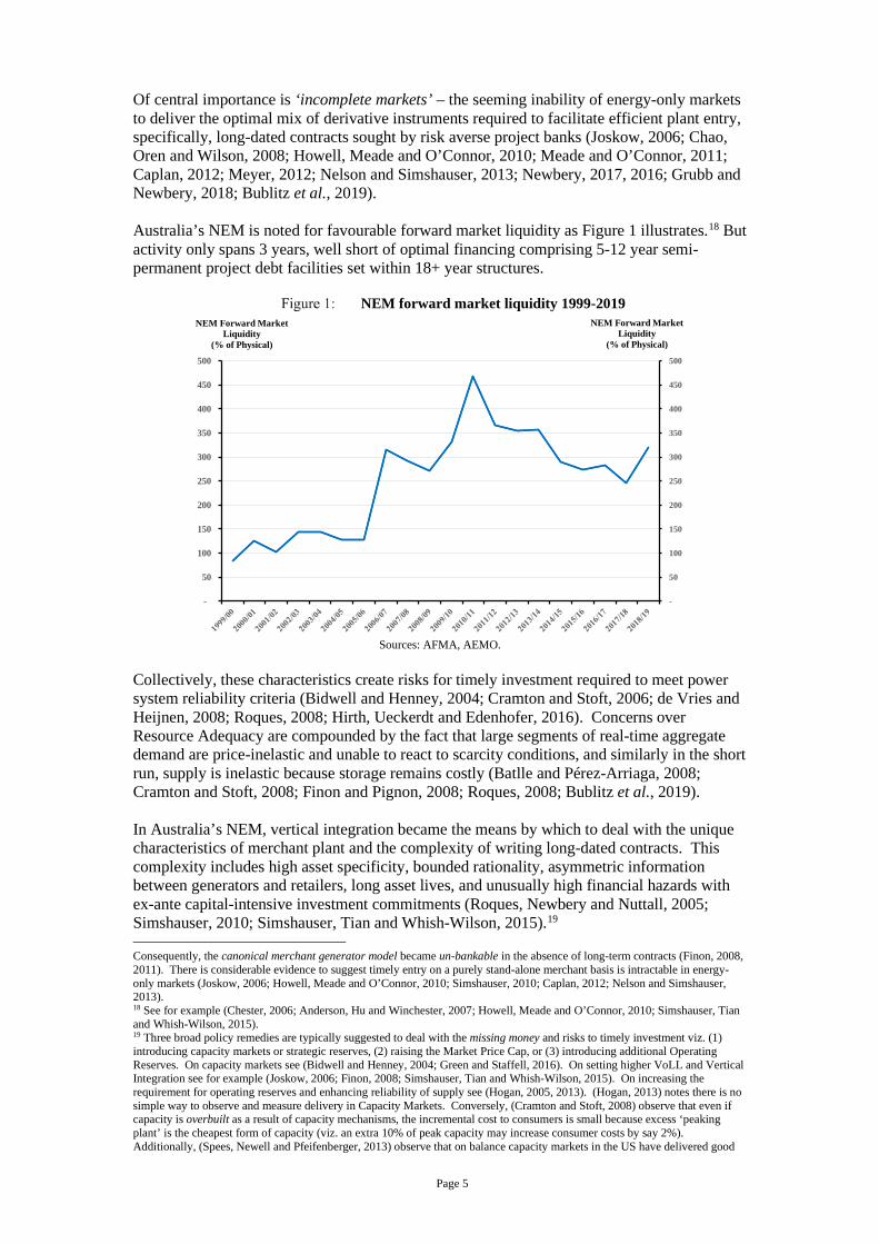
Of central importance is ‘incomplete markets’ – the seeming inability of energy-only markets to deliver the optimal mix of derivative instruments required to facilitate efficient plant entry, specifically, long-dated contracts sought by risk averse project banks (Joskow, 2006; Chao, Oren and Wilson, 2008; Howell, Meade and O’Connor, 2010; Meade and O’Connor, 2011; Caplan, 2012; Meyer, 2012; Nelson and Simshauser, 2013; Newbery, 2017, 2016; Grubb and Newbery, 2018; Bublitz et al., 2019). Australia’s NEM is noted for favourable forward market liquidity as Figure 1 illustrates.18 But activity only spans 3 years, well short of optimal financing comprising 5-12 year semi-permanent project debt facilities set within 18+ year structures.

NEM forward market liquidity 1999-2019

Sources: AFMA, AEMO.

Collectively, these characteristics create risks for timely investment required to meet power system reliability criteria (Bidwell and Henney, 2004; Cramton and Stoft, 2006; de Vries and Heijnen, 2008; Roques, 2008; Hirth, Ueckerdt and Edenhofer, 2016). Concerns over Resource Adequacy are compounded by the fact that large segments of real-time aggregate demand are price-inelastic and unable to react to scarcity conditions, and similarly in the short run, supply is inelastic because storage remains costly (Batlle and Pérez-Arriaga, 2008; Cramton and Stoft, 2008; Finon and Pignon, 2008; Roques, 2008; Bublitz et al., 2019). In Australia’s NEM, vertical integration became the means by which to deal with the unique characteristics of merchant plant and the complexity of writing long-dated contracts. This complexity includes high asset specificity, bounded rationality, asymmetric information between generators and retailers, long asset lives, and unusually high financial hazards with ex-ante capital-intensive investment commitments (Roques, Newbery and Nuttall, 2005; Simshauser, 2010; Simshauser, Tian and Whish-Wilson, 2015).19

Consequently, the canonical merchant generator model became un-bankable in the absence of long-term contracts (Finon, 2008, 2011). There is considerable evidence to suggest timely entry on a purely stand-alone merchant basis is intractable in energy-only markets (Joskow, 2006; Howell, Meade and O’Connor, 2010; Simshauser, 2010; Caplan, 2012; Nelson and Simshauser, 2013). 18 See for example (Chester, 2006; Anderson, Hu and Winchester, 2007; Howell, Meade and O’Connor, 2010; Simshauser, Tian and Whish-Wilson, 2015). 19 Three broad policy remedies are typically suggested to deal with the missing money and risks to timely investment viz. (1) introducing capacity markets or strategic reserves, (2) raising the Market Price Cap, or (3) introducing additional Operating Reserves. On capacity markets see (Bidwell and Henney, 2004; Green and Staffell, 2016). On setting higher VoLL and Vertical Integration see for example (Joskow, 2006; Finon, 2008; Simshauser, Tian and Whish-Wilson, 2015). On increasing the requirement for operating reserves and enhancing reliability of supply see (Hogan, 2005, 2013). (Hogan, 2013) notes there is no simple way to observe and measure delivery in Capacity Markets. Conversely, (Cramton and Stoft, 2008) observe that even if capacity is overbuilt as a result of capacity mechanisms, the incremental cost to consumers is small because excess ‘peaking plant’ is the cheapest form of capacity (viz. an extra 10% of peak capacity may increase consumer costs by say 2%). Additionally, (Spees, Newell and Pfeifenberger, 2013) observe that on balance capacity markets in the US have delivered good

-

50

100

150

200

250

300

350

400

450

500

-

50

100

150

200

250

300

350

400

450

500

NEM Forward Market Liquidity

(% of Physical)

NEM Forward Market Liquidity

(% of Physical)

2.2 On VRE Near-zero marginal running costs of VRE plant, subsidised through side-markets, are thought to destabilise energy-only markets through merit order effects20. The basic principle underpinning the merit order effect is (subsidised) zero marginal cost VRE plant enters at the bottom of the merit order of plant, thus shifting the long-flat base load component of a power system’s aggregate supply function to the right. Ceteris paribus, prices fall (Sensfuß et al. 2008). I will refer to this as the generalised merit order effect, i.e. plant oversupply causes prices to fall. A diverse field of literature analyses whether the cost of obtaining generalised merit order effects (i.e. side payments) are justified by falls in price.21 VRE entry produces multiple effects, over multiple time-horizons. In the NEM, the diurnal pattern of wind has an off-peak bias, and solar PV has a peak bias22. The first VRE plant installed in a large thermal system is therefore likely to earn a Dispatch-Weighted Price slightly below (wind) or well above (solar) average baseload prices (Mills, Wiser and Lawrence, 2012; Nicolosi, 2012; Hirth, 2013; Simshauser, 2018). But as more VRE plant enters a series of price and production effects become visible over the short, medium and long run – not all of these leading to lower prices. Consequently, generalised merit order effects need to be decomposed across a full energy market business cycle:

1. Holding aggregate demand constant, adding any form of new supply (VRE, coal,

nuclear, transmission interconnect) produces a merit order effect. Merit order effects are not specific to VRE (Felder, 2011; Nelson, Simshauser and Nelson, 2012). But VRE does produce unique dynamics (Hirth, 2013; Simshauser, 2018; Johnson and Oliver, 2019).

2. VRE price impression effects arise from a given technology’s correlated production, driven by cumulative ‘VRE plant on’. The first solar plant will earn a price well above baseload prices. The addition of other stochastic, but correlated plant from that asset class shifts the (short-run) aggregate supply curve to the right. This has an impressing impact – exerting a technology-specific downward pressure on spot prices at certain times (Mills, Wiser and Lawrence, 2012; Nicolosi, 2012). Consequently, Dispatch-Weighted Prices of wind or solar as an asset class can be expected to deteriorate within a region relative to base prices as more of that technology class enters (Edenhofer et al., 2013; Hirth, Ueckerdt and Edenhofer, 2016).

3. VRE stochastic production effects arise as a result of cumulative ‘VRE plant off’. When wind or solar output is low, the (short run) aggregate supply curve shifts back to the left and when combined with fluctuating demand can be expected to intensify price volatility – producing distinctly elevated prices (Clò, Cataldi and Zoppoli, 2015). Johnson and Oliver (2019) identify conditions whereby stochastic production effects dominate price impression effects.

Figure 2 depicts price impression effects from cumulative VRE solar on and stochastic production effects from cumulative VRE solar off via August 2019 average 30-minute spot price data from the NEM’s Queensland Region (i.e. high levels of utility-scale and rooftop solar PV).

results in that they met their objective function, mobilised large amounts of low cost supply including Demand Response, energy efficiency, transmission interconnection, plant upgrades, deferred retirements and environmental retrofits. 20 Various countries including Germany, Denmark, Spain, Australia and North America are now routinely experiencing negative spot prices (Bunn and Yusupov, 2015). 21 See (Sensfuß, Ragwitz and Genoese, 2008; Forrest and MacGill, 2013; Joskow, 2013; Cludius, Forrest and MacGill, 2014; Bell et al., 2015, 2017; Keay, 2016; Newbery, 2016; Green and Staffell, 2016; Hach and Spinler, 2016; Keppler, 2017; Lunackova, Prusa and Janda, 2017; Benhmad and Percebois, 2018; Bublitz et al., 2019; Johnson and Oliver, 2019). 22 Peak and off-peak being defined in the traditional sense; peak being nominally 7am-10pm working weekdays. As one Reviewer also noted, solar PV output in cold-climate countries is not well correlated with peak demand – at least by comparison to hot climate jurisdictions, such as South Australia, Queensland and California, for example.

VRE price impression effect and VRE stochastic production effect

Data: AEMO

4. Thermal plant flexibility effects amplify price impression effects. When VRE fleet

output is high and spot prices fall below unit fuel costs, thermal plant can only reduce output to minimum stable loads. Generalised merit order effects therefore comprise two distinct downward forces, price impression effects, amplified by thermal plant overproduction due to flexibility limits (Nicolosi, 2012; Bunn and Yusupov, 2015). Figure 3 illustrates flexibility effects, contrasting average August 2019 output from a 280MW coal-fired unit in Queensland (RHS axis) with average spot prices (LHS axis).

Thermal plant flexibility effect

Data: AEMO

5. Utilisation effects follow. Inflexible coal plant are adversely impacted by two forces;

i). lower average prices in the post-VRE entry environment, and ii). progressively lower output, ultimately falling to some minimum critical level (Höschle et al., 2017). Given suboptimal output levels and heavy sunk costs, coal plant begin to ‘slide up’

0

100

200

300

400

500

600

700

800

900

1000

0

20

40

60

80

100

120

140

160

Spot Price ($/MWh)

Solar PV DispatchUtility-Scale Only

(MW)

Half-hour trading interval

Solar PV OutputPrice ($/MWh)Average Price

Price Impression

Effect

Stochastic Production

Effect

Qld Region, August 2019

0

50

100

150

200

250

0

20

40

60

80

100

120

140

160

Spot Price ($/MWh)

Generation Dispatch(MW)

Half-hour trading interval

Black Coal Unit DispatchSpot PriceMarginal Running Cost

Qld Region, August 2019

~Min Stable Load

Spot Prices fall below plant Marginal Running Costs = Losses

Inflexibility further impresses spot price

Flexibility Effects

their average cost function. Simultaneously confronting falling prices, the marginal coal plant becomes sub-economic and exits (Hirth, 2013; Simshauser, 2018).

Utilisation effects are the crucial long run corollary to short/medium-run generalised merit order effects. Figure 4 illustrates Northern Power Station’s utilisation effect, the last coal plant in the NEM’s South Australian region which had historically been #1 in the merit order.

Thermal plant ‘utilisation effect’

Data: AEMO

6. Following cumulative coal plant exit, a rebound effect follows. Generalised merit

order effects associated with oversupply rapidly unwind (Felder, 2011; Nelson, Simshauser and Nelson, 2012; Hirth, 2013, 2015; Simshauser, 2018, 2019a, 2019b). To be clear, this is a long run dynamic. Figure 5, which presents NEM average annual electricity prices from 1999-2019, highlights rebound effects following the cumulative exit of 11 coal plants (~5100MW or 18% of the thermal plant stock) between 2012-2017.23

Rebound Effect24

Source: Simshauser & Gilmore (2019), ABS, AEMO.

23 The final two generators in 2016 (Northern, South Australian region) and 2017 (Hazelwood, in the Victorian region) represented a distinct tipping point in the market. 24 Note that the data in Figure 5 excludes the $23/t CO2 carbon tax applicable in 2013 and 2014.

0

50,000

100,000

150,000

200,000

250,000

300,000

350,000

400,000

2010 2011 2012 2013 2014 2015 2016

Monthly Coal Plant Production

(MWh)

-

10

20

30

40

50

60

70

80

90

100

Spot Price ($/MWh)

Financial Year

LRMC

NEM Spot

Coal Plant Exits

The combination and sequencing of these effects over a full energy market business cycle should come as no surprise (Felder, 2011; Nelson, Simshauser and Nelson, 2012; Simshauser, 2019a). After all, the purpose of VRE side-markets is to induce new entry and transition the supply-side of energy markets, includes phasing out coal plant. There is no reason to believe such policies will not be successful in the long run. This has important implications for OCGT plant valuations. 2.3 On the valuation of OCGT plant A rich and diverse literature on generation plant valuation exists, spanning technologies, financing structures and business models including merchant, tolled, and PPA-contracted assets (Gardner and Zhuang, 2000; Deng, Johnson and Sogomonian, 2001; Tseng and Barz, 2002; Hlouskova et al., 2005; Hogan, 2005; Abadie and Chamorro, 2008; Heydari and Siddiqui, 2010; Fernandes, Cunha and Ferreira, 2011; Elias, Wahab and Fang, 2016; Simshauser and Gilmore, 2019). Of central importance to the valuation of gas turbine plant is the real option value of the expected difference between the price of electricity and unit fuel costs (i.e. a function of plant heat rate and cost of natural gas) known as the Spark Spread. The range of modelled prices, price resolution, and plant valuation approaches to spread options is extensive. There are four broad streams involving the use of futures prices and/or some form of mean-reverting or random walk forecasting process (see Baker, Mayfield and Parsons, 1998; Pindyck, 1999):

1. Simple spread options using futures data, solved analytically and assuming perfect plant flexibility and plant availability (Deng, Johnson and Sogomonian, 2001; Carmona and Durrleman, 2003; Fleten and Näsäkkälä, 2010);

2. Tree methods, which emerged to solve optimal investment and unit commitment

decisions by relaxing the simplifying assumptions around physical plant characteristics and non-convexities – incorporating start-up costs, ramp rate constraints, minimum run times and random outages (Gardner and Zhuang, 2000; Tseng and Lin, 2007; Abadie and Chamorro, 2008; Elias, Wahab and Fang, 2016, 2017);

3. Real options approach incorporating Monte Carlo simulation techniques to capture underlying stochastic factors known to be important drivers of value (Tseng and Barz, 2002; Hlouskova et al., 2005; Heydari and Siddiqui, 2010; Cassano and Sick, 2013; Wang and Min, 2013; Abadie, 2015) 25; and

4. Power system simulation models or ‘structural models’ which capture system-wide plant availability and load variability driven by anthropogenic patterns and seasonality with specific results fed into a conventional Discounted Cash Flow (DCF) Model.26 Contemporary power system models simulate hundreds of generation and spot price scenarios for a given (inelastic) load curve, with an objective function of cost minimisation subject to reliability constraints. Structural models are particularly well-suited to providing insight into causes of intermediate-run fluctuations, but are data (and processing-) intensive (Pindyck, 1999).27

The modelling sequence in this research lies between the 3rd and 4th streams.

25 (Cassano and Sick, 2013) is a particularly interesting analysis where they model 2 x LM6000 and a Steam Turbine, and model all plausible operating modes (i.e. cold off, idle, open cycle and combined cycle) as a call option over the spark spread – converting the two dimensional problem into one by using the market heat rate (i.e. electricity divided by gas price) based on the principles of (Margrabe, 1978). Using a bootstrap process to simulate future heat rates, they find the average market heat rate is a good explanatory variable for the time integral of the plant operating margin. 26 Structural models in the electricity industry are typically security-constrained, unit commitment models with an engine comprising a Monte Carlo-based Linear Programme – the design of which can be traced back to the joint work by Electricite de France Chief Economist Marcel Boiteux and State Electricity Commission of Victoria Chief Engineer Dr Rob Booth – applying the principles of (Calabrese, 1947), (Boiteux, 1949), (Berrie, 1967) and (Booth, 1972). 27 And if estimates of technology long run marginal costs are comparatively stable over time, such models are capable of providing helpful insights beyond the intermediate-run. The usual caveats apply.

3. Valuation model inputs

For applied transaction purposes, plant valuation ideally involves the triangulation of three pieces of analysis; i). DCF Model based on an energy price forecast, ii). estimated replacement cost, and iii). recent comparable transactions. The purpose of this article is to focus on the first of these (i.e. modelled result) for three specific merchant business combinations:

1. new entrant 3 x 30MW aero-derivative OCGT;

2. incumbent 250MW Wind Portfolio, Annual Capacity Factor (ACF) of ~31%; and

3. integrated portfolio comprising 1). and 2). above. Generation assets are strictly merchant meaning output is sold into organised spot markets and hedged in short-term forward markets (Nelson and Simshauser, 2013; Wang and Min, 2013). There are no long-dated contracts – this includes Wind plant, its inaugural PPA is assumed to have expired. 3.1 OCGT Plant OCGT valuations in energy-only markets are complex because unlike base, semi-base and VRE plant which have relatively constant load factors, peaking duties involves extensive variations in ACFs – some years operating as little as 1% – prima facie making bankability problematic (Simshauser, 2010; Finon, 2011; Caplan, 2012; Nelson and Simshauser, 2013; Keppler, 2017; Bublitz et al., 2019; Milstein and Tishler, 2019). As Peluchon (2003, p2) noted long ago:

Peak capacity investment, especially, seems quite problematic. An investment in base generation plant is a decision that requires forecasting base future prices. An investment in peak generation plant is a decision that requires much more information as peak prices depend on base prices as well as from the future investments in every other kind of generation capacity. The revenue generated by peak plant is therefore much more hazardous than base plant, since it produces only when every other plant produces at full capacity or cannot produce. In the same way an option is said to be ‘out-of-the-money’, peak plant has a value that may change drastically with any change in the way the supply-demand balance evolves . . .

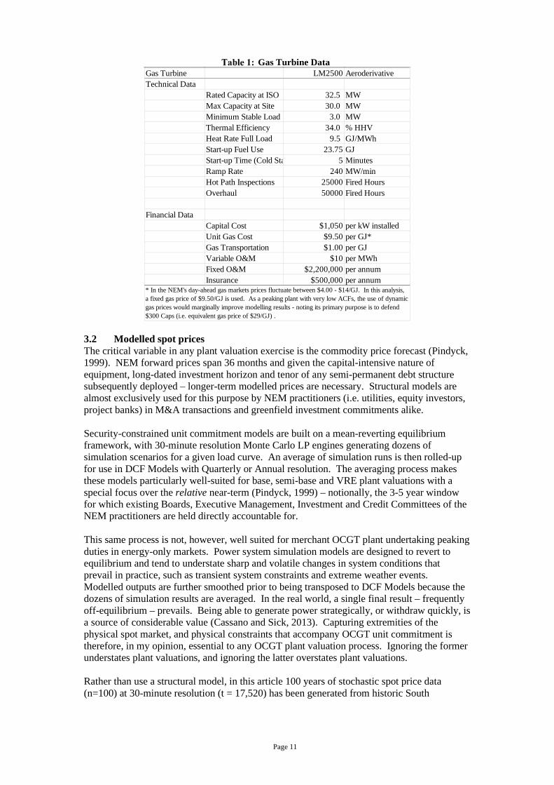
Of critical importance is the inclusion of forward contracts as these stabilise expected revenues. In the NEM, the relevant forward derivative contract is the $300 Cap28. The plant being valued is 3 x GE LM2500 gas turbines with an installed capacity of 97.5MW at ISO29, and 90MW at summer-rated site conditions (Table 1). In the circumstances, it is helpful to consider the valuation for an M&A transaction involving new plant30. Aeroderivative GTs are ideally suited for integrating with merchant wind due to their rapid starting profile – from cold iron to full load in five minutes without restriction.31 Table 1 presents relevant technical and financial data.

28 The $300 Cap is traded both on-exchange and in the Over-The-Counter market. 29 Ambient temperature, altitude and humidity affect Gas Turbine output and performance (ie. Power output is dependent on the mass flow through the compressor, and as air density decreases, more power is required to compress the same mass of air, which reduces output and thermal efficiency). Consequently, the standard reference conditions for Gas Turbine Plant (ISO 3977) are 15oC, 101.3 kPa. 30 An M&A transaction involves an overnight transaction, and thus avoids detailed construction cash flow modelling. 31 LM2500s are a mature technology with 2460 units in service globally, having collectively accumulated 92 million operating hours. My thanks to the team at GE Australia.

Gas Turbine Data

3.2 Modelled spot prices The critical variable in any plant valuation exercise is the commodity price forecast (Pindyck, 1999). NEM forward prices span 36 months and given the capital-intensive nature of equipment, long-dated investment horizon and tenor of any semi-permanent debt structure subsequently deployed – longer-term modelled prices are necessary. Structural models are almost exclusively used for this purpose by NEM practitioners (i.e. utilities, equity investors, project banks) in M&A transactions and greenfield investment commitments alike. Security-constrained unit commitment models are built on a mean-reverting equilibrium framework, with 30-minute resolution Monte Carlo LP engines generating dozens of simulation scenarios for a given load curve. An average of simulation runs is then rolled-up for use in DCF Models with Quarterly or Annual resolution. The averaging process makes these models particularly well-suited for base, semi-base and VRE plant valuations with a special focus over the relative near-term (Pindyck, 1999) – notionally, the 3-5 year window for which existing Boards, Executive Management, Investment and Credit Committees of the NEM practitioners are held directly accountable for. This same process is not, however, well suited for merchant OCGT plant undertaking peaking duties in energy-only markets. Power system simulation models are designed to revert to equilibrium and tend to understate sharp and volatile changes in system conditions that prevail in practice, such as transient system constraints and extreme weather events. Modelled outputs are further smoothed prior to being transposed to DCF Models because the dozens of simulation results are averaged. In the real world, a single final result – frequently off-equilibrium – prevails. Being able to generate power strategically, or withdraw quickly, is a source of considerable value (Cassano and Sick, 2013). Capturing extremities of the physical spot market, and physical constraints that accompany OCGT unit commitment is therefore, in my opinion, essential to any OCGT plant valuation process. Ignoring the former understates plant valuations, and ignoring the latter overstates plant valuations. Rather than use a structural model, in this article 100 years of stochastic spot price data (n=100) at 30-minute resolution (t = 17,520) has been generated from historic South

Gas Turbine LM2500 AeroderivativeTechnical Data

Rated Capacity at ISO 32.5 MWMax Capacity at Site 30.0 MWMinimum Stable Load 3.0 MWThermal Efficiency 34.0 % HHVHeat Rate Full Load 9.5 GJ/MWhStart-up Fuel Use 23.75 GJStart-up Time (Cold Sta 5 MinutesRamp Rate 240 MW/minHot Path Inspections 25000 Fired HoursOverhaul 50000 Fired Hours

Financial DataCapital Cost $1,050 per kW installedUnit Gas Cost $9.50 per GJ*Gas Transportation $1.00 per GJVariable O&M $10 per MWhFixed O&M $2,200,000 per annumInsurance $500,000 per annum

* In the NEM's day-ahead gas markets prices fluctuate between $4.00 - $14/GJ. In this analysis, a fixed gas price of $9.50/GJ is used. As a peaking plant with very low ACFs, the use of dynamic gas prices would marginally improve modelling results - noting its primary purpose is to defend $300 Caps (i.e. equivalent gas price of $29/GJ) .

Australian NEM region data.32 The benefit of using South Australian spot (and forward) data over the 10-year period 2010-2019 as a base is that the price series captures a complete energy market business cycle comprising:

1. Over-capacity and well documented merit order effects33 arising from cumulative wind and solar PV entry to world-record market shares of 50+%, and

2. severe supply-side shocks (i.e. rebound effects) arising from cumulative thermal plant

exit (see Simshauser, 2019a).

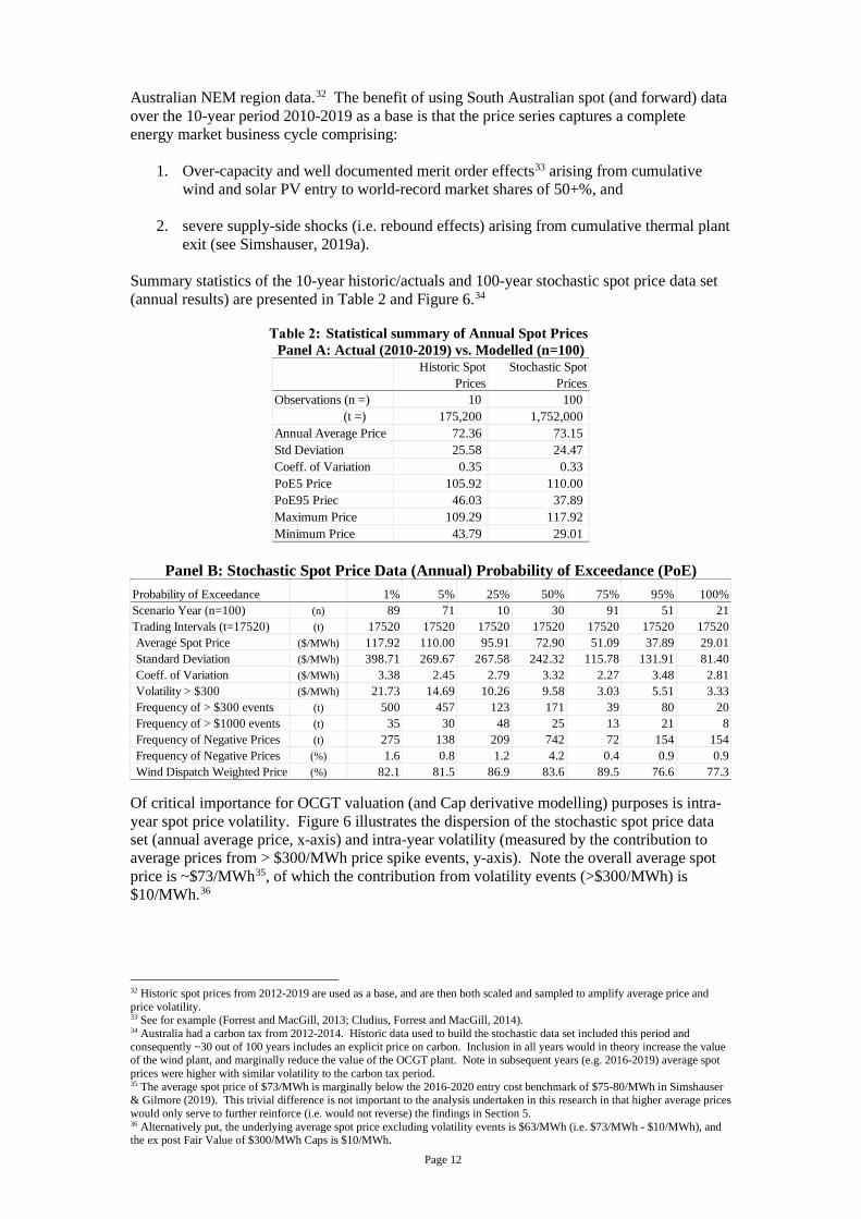
Summary statistics of the 10-year historic/actuals and 100-year stochastic spot price data set (annual results) are presented in Table 2 and Figure 6.34

Statistical summary of Annual Spot Prices Panel A: Actual (2010-2019) vs. Modelled (n=100)

Panel B: Stochastic Spot Price Data (Annual) Probability of Exceedance (PoE)

Of critical importance for OCGT valuation (and Cap derivative modelling) purposes is intra-year spot price volatility. Figure 6 illustrates the dispersion of the stochastic spot price data set (annual average price, x-axis) and intra-year volatility (measured by the contribution to average prices from > $300/MWh price spike events, y-axis). Note the overall average spot price is ~$73/MWh35, of which the contribution from volatility events (>$300/MWh) is $10/MWh.36

32 Historic spot prices from 2012-2019 are used as a base, and are then both scaled and sampled to amplify average price and price volatility. 33 See for example (Forrest and MacGill, 2013; Cludius, Forrest and MacGill, 2014). 34 Australia had a carbon tax from 2012-2014. Historic data used to build the stochastic data set included this period and consequently ~30 out of 100 years includes an explicit price on carbon. Inclusion in all years would in theory increase the value of the wind plant, and marginally reduce the value of the OCGT plant. Note in subsequent years (e.g. 2016-2019) average spot prices were higher with similar volatility to the carbon tax period. 35 The average spot price of $73/MWh is marginally below the 2016-2020 entry cost benchmark of $75-80/MWh in Simshauser & Gilmore (2019). This trivial difference is not important to the analysis undertaken in this research in that higher average prices would only serve to further reinforce (i.e. would not reverse) the findings in Section 5. 36 Alternatively put, the underlying average spot price excluding volatility events is $63/MWh (i.e. $73/MWh - $10/MWh), and the ex post Fair Value of $300/MWh Caps is $10/MWh.

Historic Spot Prices

Stochastic Spot Prices

Observations (n =) 10 100 (t =) 175,200 1,752,000 Annual Average Price 72.36 73.15 Std Deviation 25.58 24.47 Coeff. of Variation 0.35 0.33 PoE5 Price 105.92 110.00 PoE95 Priec 46.03 37.89 Maximum Price 109.29 117.92 Minimum Price 43.79 29.01

Probability of Exceedance 1% 5% 25% 50% 75% 95% 100%Scenario Year (n=100) (n) 89 71 10 30 91 51 21Trading Intervals (t=17520) (t) 17520 17520 17520 17520 17520 17520 17520Average Spot Price ($/MWh) 117.92 110.00 95.91 72.90 51.09 37.89 29.01Standard Deviation ($/MWh) 398.71 269.67 267.58 242.32 115.78 131.91 81.40Coeff. of Variation ($/MWh) 3.38 2.45 2.79 3.32 2.27 3.48 2.81Volatility > $300 ($/MWh) 21.73 14.69 10.26 9.58 3.03 5.51 3.33Frequency of > $300 events (t) 500 457 123 171 39 80 20Frequency of > $1000 events (t) 35 30 48 25 13 21 8Frequency of Negative Prices (t) 275 138 209 742 72 154 154Frequency of Negative Prices (%) 1.6 0.8 1.2 4.2 0.4 0.9 0.9Wind Dispatch Weighted Price (%) 82.1 81.5 86.9 83.6 89.5 76.6 77.3

Stochastic spot prices – Annual Average vs Annual Volatility (>$300 spikes)

3.3 Wind and Dispatch-Weighted Price For valuation purposes the wind plant is assumed to have a (depreciated) capital-cost base of $1750/kW, Fixed O&M costs of $10,000/MW installed and Variable O&M costs of $12/MWh with an average ACF of 32.1% (min 28.2% and max 33.9%). Note subsequent analysis excludes any form of side-market (i.e. Renewable Certificate37) revenues. An important variable in the subsequent analysis is the ‘earned price’ of wind turbine generators (i.e. Dispatch-Weighted Price). As an absolute general conclusion, the annual Dispatch-Weighted Price cannot be greater than the time-weighted spot price because:

• NEM wind generation output tends to have an off-peak bias; and

• When demand is higher than forecast, all else equal, dispatchable generators increase output and receive a higher average price. Conversely, stochastic generators reduce output disproportionately in periods of oversupply and hence sell at disproportionately lower prices (Joskow, 2011; Mills, Wiser and Lawrence, 2012; Edenhofer et al., 2013; Hirth, 2013; Simshauser, 2018).

Consequently, the annual Dispatch-Weighted Price will be less than 100% of the time-weighted spot price – particularly as wind market share increases.38 This critical relationship must be maintained between the 100 years of stochastic 30-minute spot price data and 30-minute wind production data. If not, wind plant valuation results will almost certainly be over-stated.39 Figure 7 confirms the Dispatch-Weighted Price of the merchant 250MW Wind ranges from 77-91% (average = 84%)40.

37 In practice this would add ~$100-$150m to plant valuations. 38 As an aside, for solar PV at-scale it is even more pronounced as Figure 2 tends to suggest. See also (Mills, Wiser and Lawrence, 2012; Nicolosi, 2012; Hirth, 2013; Simshauser, 2018). 39 I should note that there are a small number of wind farms in the NEM that have Dispatch-Weighted Prices (DWP) with near perfect correlation to baseload prices, year-on-year. I am not aware of any wind farms with a DWP materially exceeding baseload prices. 40 Dispatch-Weighted Prices (%) are based on historic data from three wind farms in South Australia over the period 2012-2019.

y = 0.1685x - 2.424R² = 0.7487

-

5

10

15

20

25

- 20 40 60 80 100 120

Volatility Value >$300 ($/MWh)

Time-Weighted Spot Price ($/MWh)

Time-Weighted Average $73/MWhVolatility Value >$300 $10/MWh

Spot Price vs Wind Portfolio Dispatch Weighted Price (% of Time Weighted)

3.4 Modelled $300 Cap Futures Incorporating forward market revenues is a critical component of any merchant plant valuation exercise. Merchant plant does not mean ‘spot sales only’. The sale of forward derivatives are essential from a cashflow management perspective, and drive unit commitment. In Australian financial markets the two most commonly traded electricity derivatives are Swaps and $300 Caps41, the latter being the forward contract of choice to manage risks associated with load uncertainty and extreme price spike events. The traded history of $300 Caps in the NEM’s SA region (daily resolution) is presented in Figure 8.

$300 Cap Futures – Calendar Year Strips 2008-2021 (constant 2019 dollars)

Source: ASX, ABS.

The theoretical equilibrium price of $300 Caps can be derived by calculating a Boiteux Capacity Payment, viz. carrying cost of an OCGT undertaking ‘reserve duties’, expressed in $ per MW per hour. Given OCGT cost data in Table 1, this equates to ~$14/MWh.42

41 $300 is a long-standing NEM convention that provides sufficient headroom for all peaking plant to be economically dispatched even if operating on liquid fuels. 42 See Simshauser & Gilmore (2019, p269) for a detailed analysis of the calculation using the ‘PF Model’ with both on- and off-Balance Sheet financing structures.

-

20

40

60

80

100

120

50% 55% 60% 65% 70% 75% 80% 85% 90% 95% 100%

Time-Weighted Spot Price ($/MWh)

Dispatch-Weighted Price (%)

0

5

10

15

20

25

30

35

$300 Cap Futures Cal Yr Strip

($/MWh) 2008 2009 2010 2011 20122013 2014 2015 2016 20172018 2019 2020 2021 AVG

Ex ante, $300 Caps trade at a premium to their ex post Fair Value – an expected result given the nature of the instrument.43 Figure 9 re-organises Figure 8 data into a ‘3-Year Accumulated Portfolio’ price trace (solid line series) over the 10-year period 2010-2019. The Accumulated Portfolio involves progressively layering Caps into a portfolio over the three-year period leading up to real-time. The 10-Year ex ante average traded Cap Price, and ex post average Cap Settlement is also illustrated (dashed and dotted line series), revealing an ex ante Cap premium of ~30%.

3-Year Accumulated Portfolio of $300 Cap & Cap Payouts (2010-2019)

Source: ASX, AEMO, ABS.

Table 3 presents a statistical summary of Traded Caps, their ex post Fair Value, and a comparison between the historic/actual 3-Year Accumulated Portfolio (2010-2019) and modelled 3-Year Accumulated Portfolio used in this research, which has been estimated via Eq.(1). Note Eq.(1) modelled prices for the Accumulated Portfolio are broadly consistent with the historic 2010-2019 Accumulated Portfolio, viz. 𝜇𝜇𝑐𝑐 ≅ $13/𝑀𝑀𝑀𝑀ℎ, 𝜎𝜎𝑐𝑐 ≅ $3/𝑀𝑀𝑀𝑀ℎ with Coefficient of Variation ~0.24.

10-Year Statistical summary of $300 Cap Strips (2010-2019) – Actual and Modelled

Source: ASX, AEMO (for Traded Caps and Fair Value ex post)

The modelled 3-Year Accumulated Portfolio of $300 Caps is tightly aligned with the stochastic spot price data set, as follows: 𝑝𝑝𝑐𝑐𝑛𝑛,𝑖𝑖 = 𝜇𝜇𝑐𝑐 − (2.25 ∙ 𝜎𝜎𝑐𝑐) + ��𝐹𝐹𝑉𝑉𝑐𝑐

𝑛𝑛−1,𝑖𝑖 + 𝐹𝐹𝑉𝑉𝑐𝑐𝑛𝑛,𝑖𝑖� 2⁄ � ∙ (1 + 𝛿𝛿𝑐𝑐) | 𝛿𝛿𝑐𝑐 = 𝜇𝜇 − 𝐹𝐹𝑉𝑉𝑐𝑐 , (1)

where: 𝑝𝑝𝑐𝑐𝑛𝑛,𝑖𝑖 = modelled prices of an Accumulated Portfolio of $300 Caps c in year n and

43 Caps are an insurance product used by Retail Suppliers to manage risk exposures associated with extreme weather events – events which by their nature are only likely to occur 1-in-10 years. For Retailers, dual-impacts of high price and high volumes raises the possibility of financial distress.

17.67 9.14 1.65 9.64 3.86 7.52 17.20 9.75 10.93 12.65

17.5116.19

15.15

11.57

9.35 8.90

10.49

14.6115.71

12.21

0

2

4

6

8

10

12

14

16

18

20

2010 2011 2012 2013 2014 2015 2016 2017 2018 2019

$300 Cap Futures($/MWh)

Calendar Year

Fair Value Ex Post (Payout)

3-Yr Accumulated Portfolio

10 Yr Average $300 Cap Price

Contract Premium ~30%

Avg of Traded $300 Caps

Fair Value $300 Cap Ex Post

2010-19 $300 Cap Accum. Portfolio

Modelled $300 Cap Accum. Portfolio

Observations 6,933 10 10 500 Average 12.84 10.00 12.98 12.91 Std Deviation 4.49 5.09 2.96 3.05 Coeff. Variation 0.35 0.51 0.23 0.24 Min 6.32 1.65 8.90 `7.46Max 29.40 17.67 17.51 `17.69`Sample results from a single 25 Year Simulation.

iteration i (and i = 1..500) 𝜇𝜇𝑐𝑐 = long run average of the 3-Year Accumulated Portfolio of $300 Caps 𝜎𝜎𝑐𝑐 = standard deviation of the 3-Year Accumulated Portfolio of $300 Caps 𝐹𝐹𝑉𝑉𝑐𝑐

𝑛𝑛,𝑖𝑖 = ex post Fair Value (i.e. payout) of $300 Caps from stochastic spot prices in year n and iteration i

𝛿𝛿𝑐𝑐 = long run observable Cap Premium (30%, per Figure 9) Figure 10 illustrates 10 samples of modelled ‘Accumulated Portfolio of $300 Caps’ traces (i.e. i=10 of 500 iterations, n=25 years, the nominal project life for valuation purposes). Cap prices ($/MWh) are measured on the y-axis for each valuation year n on the x-axis.

Modelled Accumulated Portfolio of $300 Caps vs Entry Cost (i=1..10 of 500)

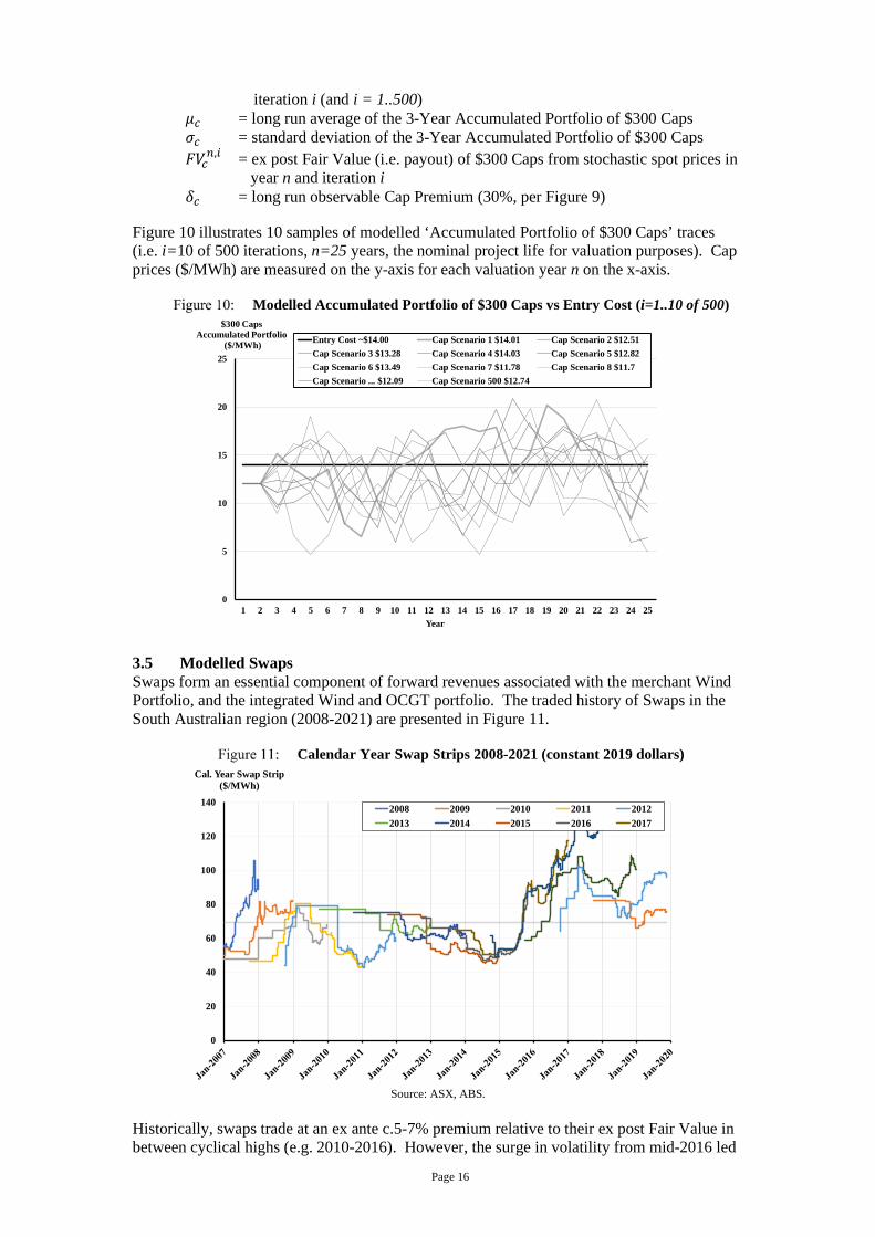
3.5 Modelled Swaps Swaps form an essential component of forward revenues associated with the merchant Wind Portfolio, and the integrated Wind and OCGT portfolio. The traded history of Swaps in the South Australian region (2008-2021) are presented in Figure 11.

Calendar Year Swap Strips 2008-2021 (constant 2019 dollars)

Source: ASX, ABS.

Historically, swaps trade at an ex ante c.5-7% premium relative to their ex post Fair Value in between cyclical highs (e.g. 2010-2016). However, the surge in volatility from mid-2016 led

0

5

10

15

20

25

1 2 3 4 5 6 7 8 9 10 11 12 13 14 15 16 17 18 19 20 21 22 23 24 25

$300 CapsAccumulated Portfolio

($/MWh)

Year

Entry Cost ~$14.00 Cap Scenario 1 $14.01 Cap Scenario 2 $12.51Cap Scenario 3 $13.28 Cap Scenario 4 $14.03 Cap Scenario 5 $12.82Cap Scenario 6 $13.49 Cap Scenario 7 $11.78 Cap Scenario 8 $11.7Cap Scenario ... $12.09 Cap Scenario 500 $12.74

0

20

40

60

80

100

120

140

Cal. Year Swap Strip ($/MWh)

2008 2009 2010 2011 20122013 2014 2015 2016 2017

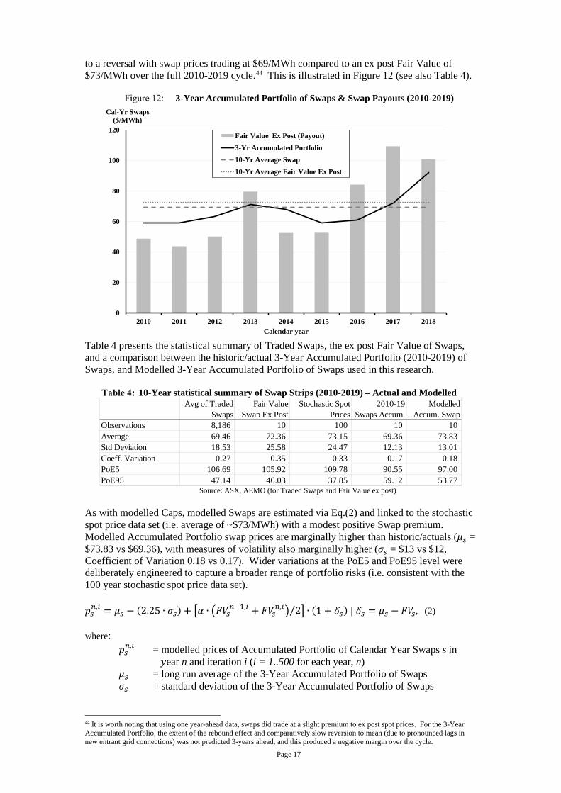
to a reversal with swap prices trading at $69/MWh compared to an ex post Fair Value of $73/MWh over the full 2010-2019 cycle.44 This is illustrated in Figure 12 (see also Table 4).

3-Year Accumulated Portfolio of Swaps & Swap Payouts (2010-2019)

Table 4 presents the statistical summary of Traded Swaps, the ex post Fair Value of Swaps, and a comparison between the historic/actual 3-Year Accumulated Portfolio (2010-2019) of Swaps, and Modelled 3-Year Accumulated Portfolio of Swaps used in this research.

10-Year statistical summary of Swap Strips (2010-2019) – Actual and Modelled

Source: ASX, AEMO (for Traded Swaps and Fair Value ex post)

As with modelled Caps, modelled Swaps are estimated via Eq.(2) and linked to the stochastic spot price data set (i.e. average of ~$73/MWh) with a modest positive Swap premium. Modelled Accumulated Portfolio swap prices are marginally higher than historic/actuals (𝜇𝜇𝑠𝑠 = $73.83 vs $69.36), with measures of volatility also marginally higher (𝜎𝜎𝑠𝑠 = $13 vs $12, Coefficient of Variation 0.18 vs 0.17). Wider variations at the PoE5 and PoE95 level were deliberately engineered to capture a broader range of portfolio risks (i.e. consistent with the 100 year stochastic spot price data set). 𝑝𝑝𝑠𝑠𝑛𝑛,𝑖𝑖 = 𝜇𝜇𝑠𝑠 − (2.25 ∙ 𝜎𝜎𝑠𝑠) + �𝛼𝛼 ∙ �𝐹𝐹𝑉𝑉𝑠𝑠

𝑛𝑛−1,𝑖𝑖 + 𝐹𝐹𝑉𝑉𝑠𝑠𝑛𝑛,𝑖𝑖� 2⁄ � ∙ (1 + 𝛿𝛿𝑠𝑠) | 𝛿𝛿𝑠𝑠 = 𝜇𝜇𝑠𝑠 − 𝐹𝐹𝑉𝑉𝑠𝑠 , (2)

where: 𝑝𝑝𝑠𝑠𝑛𝑛,𝑖𝑖 = modelled prices of Accumulated Portfolio of Calendar Year Swaps s in

𝑦𝑦ear n and iteration i (i = 1..500 for each year, n) 𝜇𝜇𝑠𝑠 = long run average of the 3-Year Accumulated Portfolio of Swaps 𝜎𝜎𝑠𝑠 = standard deviation of the 3-Year Accumulated Portfolio of Swaps

44 It is worth noting that using one year-ahead data, swaps did trade at a slight premium to ex post spot prices. For the 3-Year Accumulated Portfolio, the extent of the rebound effect and comparatively slow reversion to mean (due to pronounced lags in new entrant grid connections) was not predicted 3-years ahead, and this produced a negative margin over the cycle.

0

20

40

60

80

100

120

2010 2011 2012 2013 2014 2015 2016 2017 2018

Cal-Yr Swaps ($/MWh)

Calendar year

Fair Value Ex Post (Payout)3-Yr Accumulated Portfolio10-Yr Average Swap10-Yr Average Fair Value Ex Post

Avg of Traded Swaps

Fair Value Swap Ex Post

Stochastic Spot Prices

2010-19 Swaps Accum.

Modelled Accum. Swap

Observations 8,186 10 100 10 10 Average 69.46 72.36 73.15 69.36 73.83 Std Deviation 18.53 25.58 24.47 12.13 13.01 Coeff. Variation 0.27 0.35 0.33 0.17 0.18 PoE5 106.69 105.92 109.78 90.55 97.00 PoE95 47.14 46.03 37.85 59.12 53.77

𝛼𝛼 = estimated Swap coefficient of 0.7545 𝐹𝐹𝑉𝑉𝑠𝑠𝑛𝑛 = ex post Fair Value of Swaps from stochastic spot prices in

year n and iteration i 𝛿𝛿𝑠𝑠 = expected long run Swap Premium (set to 1%)

4. Models

Plant valuations require integration of two sequential models, i). Unit Commitment Model, and ii). Stochastic DCF Valuation Model. As (Hlouskova et al., 2005) explain when operational constraints are put aside, the problem at hand for the Unit Commitment Model is a simple one. In each trading interval:

𝑖𝑖𝑖𝑖 𝑝𝑝𝑒𝑒 �> 𝑀𝑀𝑅𝑅𝐶𝐶, 𝑞𝑞 = 𝑞𝑞� < 𝑀𝑀𝑅𝑅𝐶𝐶, 𝑞𝑞 = 0, (3)

where:

𝑝𝑝𝑒𝑒 is the spot price of electricity, 𝑀𝑀𝑅𝑅𝐶𝐶 are Marginal Running Costs, 𝑞𝑞 is quantity produced, 𝑞𝑞� is maximum continuous rating.

Gross profit 𝜋𝜋 in each trading interval must capture the real option value of the spark spread, viz. turning the OCGT on and producing to physically back forward derivatives 𝑣𝑣 sold at contract strike price 𝑝𝑝𝑐𝑐, or alternatively, turning the OCGT off and exhausting gains from exchange in organised spot markets46:

𝑖𝑖𝑖𝑖 𝑝𝑝𝑒𝑒 �> 𝑀𝑀𝑅𝑅𝐶𝐶,𝜋𝜋 = 𝑣𝑣(𝑝𝑝𝑐𝑐 − 𝑀𝑀𝑅𝑅𝐶𝐶) + (𝑞𝑞� − 𝑣𝑣) ∙ �𝑝𝑝𝑒𝑒 − 𝑀𝑀𝑅𝑅𝐶𝐶�< 𝑀𝑀𝑅𝑅𝐶𝐶,𝜋𝜋 = 𝑣𝑣�𝑝𝑝𝑐𝑐 − 𝑝𝑝𝑒𝑒�,

(4)

Of course, gas turbine unit commitment decisions are characterised by numerous constraints and non-convexities including start-up costs47, start-up times, ramp-rate, minimum stable loads, minimum run-times, planned inspections and forced outages. Axiomatically, in energy-only markets with a high Market Price Cap, failing to capture these over-values OCGT plant, hence the purpose of a Unit Commitment Model. 4.1 Unit Commitment Model The Model simulates plant dispatch with an objective function of maximising spread options inherent in spot prices subject to the various constraints and non-convexities that characterise OCGT plant. Essential model inputs include gas turbine technical and financial data (Table 1), and the 30-minute spot price data array. Model structure is as follows: Let Y be the ordered set of Years. 𝑛𝑛 ∈ {1. . |𝑌𝑌|} ∧ 𝑦𝑦𝑛𝑛 ∈ 𝑌𝑌, (5) Let H be the ordered set of Half-Hour trading intervals in each year 𝑛𝑛. 𝑡𝑡 ∈ {1. . |𝐻𝐻|} ∧ ℎ𝑡𝑡 ∈ 𝐻𝐻, (6) Let 𝑄𝑄� be the ordered set of gas turbine units on site at their maximum continuous rating. 𝑗𝑗 ∈ {1. . |𝑄𝑄�|} ∧ 𝑞𝑞�𝑗𝑗 ∈ 𝑄𝑄� , (7)

45 As with Eq.(1), the second term in Eq.(2) ensures there is no systematic bias towards ‘more hedging’ given 𝛿𝛿𝑠𝑠 is non-negative. In Eq.(2) the addition 𝛼𝛼 coefficient (i.e. at 0.75) in the estimation process ensures the overall average is ~$73/MWh. 46 The structure of Eq.(4) implies forward derivatives are Swaps rather than Caps. To convert to Caps, premia needs to be included in each trading interval. 47 The maintenance regime of Frame gas turbines undertaking peaking duties are driven by the number of unit starts. Maintenance of aeroderivative gas turbines are driven by running hours. Both technologies use additional fuel during start-up.

Let 𝐾𝐾 be the ordered set of wind turbines. 𝑤𝑤 ∈ {1. . |𝐾𝐾|} ∧ 𝑘𝑘𝑤𝑤 ∈ 𝐾𝐾, (8) Marginal Running Costs include Fuel 𝐹𝐹�𝑞𝑞𝑗𝑗𝑡𝑡� and Variable Operations & Maintenance costs �𝑉𝑉𝐶𝐶𝑀𝑀𝑗𝑗

𝑡𝑡�. Fuel 𝐹𝐹�𝑞𝑞𝑗𝑗𝑡𝑡� is non-convex because of start-up quantity 𝑎𝑎𝑗𝑗 with marginal fuel consumed at the plant’s heat rate ℎ𝑗𝑗. Each coefficient is strictly non-negative. 𝑝𝑝𝑓𝑓𝑡𝑡 is the price of fuel. Once operational, 𝑀𝑀𝑅𝑅𝐶𝐶𝑗𝑗𝑡𝑡 reduces because Fuel consumed during the start-up sequence �𝑎𝑎𝑗𝑗� is sunk.

∃ 𝑞𝑞�𝑗𝑗 �𝑀𝑀𝑅𝑅𝐶𝐶𝑗𝑗𝑡𝑡 = 𝐹𝐹 �𝑞𝑞𝑗𝑗𝑡𝑡� ∙ 𝑝𝑝𝑖𝑖

𝑡𝑡 − 𝑞𝑞𝑗𝑗𝑡𝑡 ∙ 𝑉𝑉𝐶𝐶𝑀𝑀𝑗𝑗

𝑡𝑡 � 𝐹𝐹 �𝑞𝑞𝑗𝑗𝑡𝑡� = 𝑖𝑖𝑖𝑖 �

𝑞𝑞𝑗𝑗𝑡𝑡−1 = 0, 𝑎𝑎𝑗𝑗 + ℎ𝑗𝑗 ∙ 𝑞𝑞𝑗𝑗

𝑡𝑡

𝑞𝑞𝑗𝑗𝑡𝑡−1 > 0, ℎ𝑗𝑗 ∙ 𝑞𝑞𝑗𝑗

𝑡𝑡, (9)

Following unit commitment, quantity produced 𝑞𝑞𝑗𝑗𝑡𝑡 is bounded by maximum rated capacity 𝑞𝑞�𝑗𝑗 and minimum stable load 𝑞𝑞𝑗𝑗. 𝑞𝑞𝐽𝐽 < 𝑞𝑞𝑗𝑗𝑡𝑡 < 𝑞𝑞�𝑗𝑗 ∀ 𝑞𝑞𝑗𝑗𝑡𝑡 > 0, (10) Plant is subject to planned �𝑉𝑉𝑗𝑗,𝑢𝑢

𝑡𝑡 � and forced �𝛼𝛼𝑗𝑗,𝑢𝑢𝑡𝑡 � outages of one week and 6% per annum

respectively. Planned outages are pre-scheduled in mild seasons. Forced outages (including failed starts) are random, occurring throughout the year. Available capacity is therefore stochastic and modelled at the station level for each trading interval:

∑ 𝑞𝑞𝑗𝑗𝑡𝑡|𝑄𝑄�|

𝑗𝑗=1 | 𝑖𝑖𝑖𝑖 �𝑟𝑟𝑎𝑎𝑛𝑛𝑟𝑟[0. .1] < 𝛼𝛼𝑗𝑗,𝑢𝑢

𝑡𝑡 ⋀ 𝑡𝑡 ≠ 𝑉𝑉𝑗𝑗,𝑢𝑢𝑡𝑡 , 𝑞𝑞𝑗𝑗

𝑡𝑡

𝑟𝑟𝑎𝑎𝑛𝑛𝑟𝑟[0. .1] ≥ 𝛼𝛼𝑗𝑗,𝑢𝑢𝑡𝑡 ⋁ 𝑡𝑡 = 𝑉𝑉𝑗𝑗,𝑢𝑢

𝑡𝑡 , 0, (11)

Gas turbines are subject to a start-up sequence�𝛾𝛾𝑗𝑗� which means maximum output in the first trading interval following unit commitment is not feasible:

𝑖𝑖𝑖𝑖 𝑝𝑝𝑒𝑒𝑡𝑡 > 𝑀𝑀𝑅𝑅𝐶𝐶𝑗𝑗𝑡𝑡 ∧ 𝑞𝑞𝑗𝑗𝑡𝑡−1 �

= 0, �𝛾𝛾𝑗𝑗 ∙ 𝑞𝑞𝑡𝑡�

≠ 0, 𝑞𝑞𝑡𝑡, (12)

Gas turbines have practical minimum economic run-times. Unit commitment is subject to expected electricity prices 𝑝𝑝𝑒𝑒𝑡𝑡 over a look-ahead period (𝑙𝑙) nominally set to two hours to ensure units are not started for brief periods of marginal value.48 Conversely, if already operational and marginal value is expected, units remain in service:

𝑞𝑞𝑗𝑗𝑡𝑡 = 𝑖𝑖𝑖𝑖 �∑ 𝑝𝑝𝑒𝑒𝑡𝑡

𝑙𝑙𝑡𝑡+𝑙𝑙t ≥ MRC𝑗𝑗𝑡𝑡,𝑞𝑞

𝑡𝑡

𝑞𝑞𝑡𝑡−1 > 0 ∧ 𝑝𝑝𝑒𝑒𝑡𝑡 ≥ MRC𝑗𝑗𝑡𝑡,𝑞𝑞𝑡𝑡

𝐶𝐶𝑡𝑡ℎ𝑒𝑒𝑟𝑟𝑤𝑤𝑖𝑖𝑒𝑒𝑒𝑒 0.

(13)

In the present exercise, key financial and operational outputs for each trading interval t in each year n are extracted and rolled-up into an ordered set of annual results (𝑛𝑛 = 100). Operational Results Operational results include plant output (𝑄𝑄𝑛𝑛), unit starts 𝑈𝑈𝑛𝑛, fuel consumed 𝐹𝐹(𝑄𝑄𝑛𝑛) and plant operating hours 𝑈𝑈𝐶𝐶𝐻𝐻𝑛𝑛.

48 The consequence of Eq.(13) is that the station will sometimes start early in anticipation of a major price spike thereby capturing realistic behaviour under uncertainty, and may not generate during brief spikes of low profitability thereby avoiding unnecessary operating hours and/or unit starts. However, subject to Eq.(11) unit commitment will always hit major price spikes reflecting an assumption of high quality short-term price forecasting.

𝑄𝑄𝑛𝑛 = ∑ ∑ 𝑞𝑞𝑗𝑗𝑡𝑡|𝐻𝐻|𝑡𝑡=1

|𝑄𝑄|𝑗𝑗=1 , (14)

𝑈𝑈𝑛𝑛 = ∑ ∑ 𝑒𝑒𝑗𝑗𝑡𝑡|𝐻𝐻|𝑡𝑡=1

|𝑄𝑄|𝑗𝑗=1 | 𝑖𝑖𝑖𝑖 𝑒𝑒𝑗𝑗

𝑡𝑡 = �1, 𝑞𝑞𝑗𝑗

𝑡𝑡 > 0 𝑎𝑎𝑛𝑛𝑟𝑟 𝑞𝑞𝑗𝑗𝑡𝑡−1 = 0

0, (15)

𝐹𝐹(𝑄𝑄𝑛𝑛) = 𝑎𝑎𝑗𝑗 ∙ 𝑈𝑈𝑛𝑛 + ℎ𝑗𝑗 ∙ 𝑄𝑄𝑛𝑛 , (16)

𝑈𝑈𝐶𝐶𝐻𝐻𝑛𝑛 = ∑ ∑ 𝑒𝑒𝑉𝑉ℎ𝑗𝑗𝑡𝑡|𝐻𝐻|

𝑡𝑡=1|𝑄𝑄|𝑗𝑗=1 | 𝑖𝑖𝑖𝑖 𝑞𝑞𝑗𝑗

𝑡𝑡 �> 0,𝑒𝑒𝑉𝑉ℎ𝑗𝑗

𝑡𝑡 = (1 ⋅ 𝑇𝑇)

0, 𝑒𝑒𝑉𝑉ℎ𝑗𝑗𝑡𝑡 = 0,

(17)

where 𝑇𝑇 = 0.5, given 30-minute dispatch intervals. Financial Results OCGT Net Revenue (𝑅𝑅n) are derived from electricity spot sales (𝑟𝑟𝑚𝑚𝑛𝑛), plus cap sales (𝑟𝑟𝑐𝑐𝑛𝑛), less cap payouts (𝑟𝑟𝑐𝑐𝑝𝑝𝑛𝑛 ), less Marginal Running Costs. Net Revenues are determined for each of the 100 years of results via Eq. (18)-(21). 𝑟𝑟𝑚𝑚𝑛𝑛 = ∑ ∑ �𝑞𝑞𝑗𝑗𝑡𝑡 ∙ 𝑝𝑝𝑒𝑒

𝑡𝑡 ∙ 𝑇𝑇�,|𝐻𝐻|𝑡𝑡=1

|𝑄𝑄|𝑗𝑗=1 (18)

𝑟𝑟𝑐𝑐𝑛𝑛 = ∑ ∑ �𝑣𝑣𝑐𝑐𝑛𝑛 ∙ 𝑝𝑝𝑐𝑐

𝑛𝑛 ∙ 𝑇𝑇�,|𝐻𝐻|𝑡𝑡=1

|𝑄𝑄|𝑗𝑗=1 (19)

𝑟𝑟𝑐𝑐𝑝𝑝𝑛𝑛 = ∑ [𝑚𝑚𝑎𝑎𝑥𝑥(0,𝑝𝑝𝑒𝑒𝑡𝑡 − 𝑝𝑝𝑠𝑠𝑡𝑡𝑠𝑠𝑖𝑖𝑠𝑠𝑒𝑒) ∙ 𝑣𝑣𝑐𝑐𝑛𝑛 ∙ 𝑇𝑇],|𝐻𝐻|

𝑡𝑡=1 (20) 𝑅𝑅𝑛𝑛 = 𝑟𝑟𝑚𝑚𝑛𝑛 + 𝑟𝑟𝑐𝑐𝑛𝑛 − 𝑟𝑟𝑐𝑐𝑝𝑝𝑛𝑛 − �∑ ∑ 𝑀𝑀𝑅𝑅𝐶𝐶𝑗𝑗𝑡𝑡

|𝐻𝐻|𝑡𝑡=1

|𝑄𝑄|𝑗𝑗=1 �, (21)

where 𝑣𝑣𝑐𝑐𝑛𝑛 = volume of caps sold (MW) p𝑐𝑐𝑛𝑛 = price of caps sold ($/MWh) 𝑇𝑇 = duration of each time period t (in hours) 𝑝𝑝𝑠𝑠𝑡𝑡𝑠𝑠𝑖𝑖𝑠𝑠𝑒𝑒 = strike price of cap contracts ($/MWh) For merchant wind plant, Net Revenues (𝑋𝑋𝑛𝑛) comprise spot market revenues (𝑥𝑥𝑚𝑚𝑛𝑛 ) and difference payments from Swap sales (𝑥𝑥𝑠𝑠𝑛𝑛): 𝑥𝑥𝑚𝑚𝑛𝑛 = ∑ ∑ �𝑞𝑞𝑗𝑗𝑡𝑡 ∙ 𝑝𝑝𝑒𝑒

𝑡𝑡 ∙ 𝑇𝑇�,|𝐻𝐻|𝑡𝑡=1

|𝐾𝐾|𝑤𝑤=1 (22)

𝑥𝑥𝑠𝑠𝑛𝑛 = ∑ ∑ �𝑣𝑣𝑠𝑠𝑛𝑛 ∙ �𝑝𝑝𝑒𝑒

𝑡𝑡 − 𝑝𝑝𝑒𝑒𝑛𝑛� ∙ 𝑇𝑇�,|𝐻𝐻|

𝑡𝑡=1|𝐾𝐾|𝑤𝑤=1 (23)

𝑋𝑋𝑛𝑛 = 𝑥𝑥𝑚𝑚𝑛𝑛 + 𝑥𝑥𝑠𝑠𝑛𝑛 − �∑ ∑ 𝑀𝑀𝑅𝑅𝐶𝐶𝑤𝑤𝑡𝑡

|𝐻𝐻|𝑡𝑡=1

|𝐾𝐾|𝑤𝑤=1 � | 𝑀𝑀𝑅𝑅𝐶𝐶𝑤𝑤𝑡𝑡 = �𝑞𝑞𝑤𝑤

𝑡𝑡 ∙ 𝑉𝑉𝐶𝐶𝑀𝑀𝑤𝑤𝑡𝑡 × 𝑇𝑇�. (24)

where 𝑣𝑣𝑠𝑠𝑛𝑛 = volume of swaps sold (MW) 𝑝𝑝𝑠𝑠𝑛𝑛 = price of swaps sold ($/MWh) 4.2 Stochastic DCF Valuation Model The basic structure of the Stochastic DCF Valuation Model aligns with a conventional unlevered, post-tax nominal DCF Model with 25 years duration (n =1..25), 12% expected equity returns and 6% debt finance (i.e. 9.3% and 2.4% real post-tax, respectively), 30% corporate taxes and imputed capital structure of 40/60 debt/equity. The Model uses a Monte Carlo engine and sub-sampling process to randomly populate each future year n from the 100-year array contained in the Unit Commitment Model thus generating an inherently volatile price and production series that captures full business cycle data inherent in spot and forward

energy markets (for example, see Figure 10 Cap price traces). The Monte Carlo engine is iterated 500 times (i = 500) to produce 500 distinct plant valuations and a valuation distribution similar to (Hlouskova et al., 2005). OCGT Valuation Model The ith valuation of Plant Q is calculated as follows: 𝑉𝑉𝑄𝑄𝑖𝑖 = 𝑃𝑃𝑉𝑉𝑄𝑄𝑖𝑖 ∑ �𝑟𝑟𝑚𝑚𝑛𝑛,𝑖𝑖 + 𝑟𝑟𝑐𝑐𝑛𝑛,𝑖𝑖 − 𝑟𝑟𝑐𝑐𝑝𝑝𝑛𝑛,𝑖𝑖 − �∑ ∑ 𝑀𝑀𝑅𝑅𝐶𝐶𝑗𝑗

𝑡𝑡,𝑖𝑖|𝐻𝐻|𝑡𝑡=1

|𝑄𝑄|𝑗𝑗=1 � − 𝐹𝐹𝐶𝐶𝑄𝑄𝑛𝑛 − 𝜏𝜏𝑛𝑛,𝑖𝑖� ,25

𝑛𝑛=1 (25) where

𝑉𝑉𝑄𝑄𝑖𝑖 = (Present) Value of OCGT (ith iteration) 𝐹𝐹𝐶𝐶𝑄𝑄𝑛𝑛 = Fixed Costs (i.e. Fixed Operations & Maintenance, Insurances etc) 𝜏𝜏𝑛𝑛,𝑖𝑖 = Cash taxes payable

The mid-point valuation of 500 iterations is therefore: 𝑉𝑉𝑄𝑄 = 𝑃𝑃𝑉𝑉𝑄𝑄 ∑ �∑ �𝑟𝑟𝑚𝑚𝑛𝑛,𝑖𝑖 + 𝑟𝑟𝑐𝑐𝑛𝑛,𝑖𝑖 − 𝑟𝑟𝑐𝑐𝑝𝑝𝑛𝑛,𝑖𝑖 − �∑ ∑ 𝑀𝑀𝑅𝑅𝐶𝐶𝑗𝑗

𝑡𝑡,𝑖𝑖|𝐻𝐻|𝑡𝑡=1

|𝑄𝑄|𝑗𝑗=1 � − 𝐹𝐹𝐶𝐶𝑄𝑄𝑛𝑛 − 𝜏𝜏𝑛𝑛,𝑖𝑖�25

𝑛𝑛=1 �500𝑖𝑖=1 𝑖𝑖⁄ , (26)

Merchant Wind Valuation Model The ith valuation of Portfolio K is calculated as follows: 𝑉𝑉𝐾𝐾𝑖𝑖 = 𝑃𝑃𝑉𝑉𝐾𝐾𝑖𝑖 ∑ �𝑥𝑥𝑚𝑚𝑛𝑛,𝑖𝑖 + 𝑥𝑥𝑒𝑒𝑛𝑛,𝑖𝑖 − �∑ ∑ 𝑀𝑀𝑅𝑅𝐶𝐶𝑤𝑤𝑡𝑡,𝑖𝑖|𝐻𝐻|

𝑡𝑡=1|𝐾𝐾|𝑤𝑤=1 � − 𝐹𝐹𝐶𝐶𝐾𝐾𝑛𝑛 − 𝜏𝜏𝑛𝑛,𝑖𝑖�25

𝑛𝑛=1 , (27) where

𝑃𝑃𝑉𝑉𝐾𝐾𝑖𝑖 = Present Value of Wind plant (ith iteration) 𝐹𝐹𝐶𝐶𝐾𝐾𝑛𝑛 = Wind plant Fixed Costs

The mid-point valuation follows the same procedure as Eq.(26). Merchant Wind & Gas Turbine Valuation Model - Optimisation Integration of merchant wind and OCGT plant requires stand-alone hedge portfolios to be re-organised. Specifically, optimal swap levels are increased to average portfolio output, with Cap derivatives reduced to enable the OCGT plant to form a real option against Swaps in light of intermittent output. The volume and structure of portfolio derivatives 𝐷𝐷𝑛𝑛 is therefore: 𝐷𝐷𝑛𝑛 = �̀�𝑣𝑠𝑠 + �̀�𝑣c | �̀�𝑣𝑠𝑠 ≅ 𝑒𝑒(𝑃𝑃𝑉𝑉𝑟𝑟𝑡𝑡𝑖𝑖𝑉𝑉𝑙𝑙𝑖𝑖𝑉𝑉 𝐴𝐴𝐶𝐶𝐹𝐹) ∀ 𝑛𝑛 ∧ �̀�𝑣c = max(0,𝑣𝑣𝑐𝑐 − 𝑣𝑣𝑠𝑠) ∀ 𝑛𝑛, (28) where ex ante, expected average portfolio output is ~80MW.49 The ith valuation of the Portfolio therefore is: 𝑉𝑉𝐾𝐾,𝑊𝑊𝑖𝑖 = 𝑃𝑃𝑉𝑉𝐾𝐾,𝑊𝑊

𝑖𝑖 ∑ ��𝑟𝑟𝑚𝑚𝑛𝑛,𝑖𝑖 + 𝑥𝑥𝑚𝑚𝑛𝑛,𝑖𝑖� + ��̀�𝑥𝑒𝑒𝑛𝑛,𝑖𝑖 + �̀�𝑟𝑐𝑐𝑛𝑛,𝑖𝑖 − �̀�𝑟𝑐𝑐𝑝𝑝𝑛𝑛,𝑖𝑖� − ��∑ ∑ 𝑀𝑀𝑅𝑅𝐶𝐶𝑗𝑗𝑡𝑡,𝑖𝑖|𝐻𝐻|

𝑡𝑡=1|𝑄𝑄|𝑗𝑗=1 � +25

𝑛𝑛=1

�∑ ∑ 𝑀𝑀𝑅𝑅𝐶𝐶𝑤𝑤𝑡𝑡,𝑖𝑖|𝐻𝐻|𝑡𝑡=1

|𝐾𝐾|𝑤𝑤=1 �� − ∑𝐹𝐹𝐶𝐶𝑄𝑄,𝐾𝐾

𝑛𝑛 − 𝜏𝜏𝑛𝑛,𝑖𝑖�. (29) The mid-point valuation follows the same procedure as Eq.(26). 5. Modelling Results

A rising view in energy economics and policy literature is OCGT plant are increasingly unprofitable due to VRE merit order effects and lower run times, implying capacity markets or strategic reserves may be essential (Hach and Spinler, 2016; Höschle et al., 2017; Bublitz et al., 2019; Milstein and Tishler, 2019). But recall from Section 2:

49 The level of hedging would ideally be optimised for expected changes in quarterly conditions rather than limited to pre-set annual hedge levels over a 25 year period. However, this simplifying assumption reduces calculations across the 25 years x 500 iterations considerably.

1. energy-only markets have always been ‘tough neighbourhoods’ from an investment commitment perspective, especially peaking plant (Peluchon, 2003; Bidwell and Henney, 2004; Finon, 2008);

2. vertical integration has historically provided a means by which firms could navigate missing money and forward market imperfections (Simshauser, 2010; Simshauser, Tian and Whish-Wilson, 2015; Newbery, 2016);

3. merit order effects have multiple dimensions over multiple timeframes (Hirth, 2013; Hirth, Ueckerdt and Edenhofer, 2016) and eventually produce near-perfect market conditions for OCGT plant entry; and

4. merchant stochastic VRE plant are analogous to, or a mirror image of, stochastic loads. Consequently, integration of merchant VRE plant with OCGT plant should also, in theory, present transactional gains.

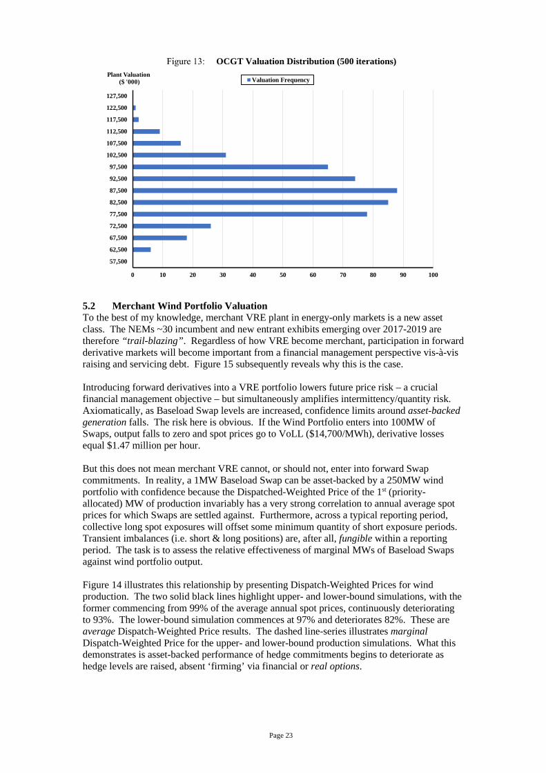
Testing this concept requires three sequential valuations i). merchant OCGT plant, ii). merchant Wind Portfolio, and iii). an integrated portfolio comprising i) and ii). The marginal value of the integrated portfolio result can be quickly derived by comparison with the Sum-of-the-Parts, i.e. iii). vs. (i) + (ii). 5.1 OCGT Valuation Recall the OCGT plant has an overnight capital cost of ~$1050/kW or $102.3m.50 Applying the Section 3 data and Section 4 modelling sequence produces the OCGT plant valuation distribution outlined in Table 5 and Figure 13.

OCGT valuation results

The midpoint valuation is $88.6 million with PoE5 and PoE95 valuations of $105.4m and $71.6, respectively. PoE50 Annual Cash Flows (i.e. ∑ ∑ = 1250025

𝑛𝑛=1 𝑒𝑒𝑖𝑖𝑚𝑚𝑠𝑠𝑙𝑙𝑎𝑎𝑡𝑡𝑒𝑒𝑟𝑟 𝑦𝑦𝑒𝑒𝑎𝑎𝑟𝑟𝑒𝑒500𝑖𝑖=1 ) is

$9.8 million per annum, and the PoE95 result is $4.3 million. Even after accounting for a portfolio of $300 Cap derivatives, annual cash flow variations demonstrate why raising debt against a stand-alone OCGT plant is challenging. OCGT production duties are also summarised in Table 5 – average ACF is 7.9% or 692 operating hours (233 starts per unit) with significant inter-year variation. During cyclical market highs, OCGT duties surge to 24.5% ACF, and fall to just 75 Operating Hours (0.9% ACF) during market lows. Of critical importance is the mid-point OCGT plant valuation ($88.6 million) relative to entry costs of $102.3 million – a shortfall of -$13.7m (-13.4%).51 Given the nature of DCF Models, stand-alone investment commitment in new OCGT plant is more likely to occur during cyclical market highs.

50 That is, 3 x 32.5MW x $1050/kW = $102.3 million or ~US$69m. 51 This result is to be expected – recall plant entry costs are ~$14/MWh and modelled Caps are ~$13/MWh over the cycle.

3 x 30MW OCGT Plant Valuation ACF Unit Starts Op. Hours($m) (%) (#) (Hrs)

Plant Valuation (Avg of 500 iterations) 88.6 7.9 233 692 PoE5 Valuation 105.4 10.4 824 915 PoE95 Valuation 71.6 5.7 107 497 Minimum Valuation` 57.7 0.9 35 75 Maximum Valuation` 117.3 24.5 912 2,147 Avg Annual Cash Flow (500 iterations) 9.8 7.9 233 692 PoE95 Cash Flow (500 iterations) 4.3 5.7 107 497 ` Min and Max Annual Capacity Factor, Unit Starts and Operating Hour results are for a single year. Valuations relate to 25 years.

OCGT Valuation Distribution (500 iterations)

5.2 Merchant Wind Portfolio Valuation To the best of my knowledge, merchant VRE plant in energy-only markets is a new asset class. The NEMs ~30 incumbent and new entrant exhibits emerging over 2017-2019 are therefore “trail-blazing”. Regardless of how VRE become merchant, participation in forward derivative markets will become important from a financial management perspective vis-à-vis raising and servicing debt. Figure 15 subsequently reveals why this is the case. Introducing forward derivatives into a VRE portfolio lowers future price risk – a crucial financial management objective – but simultaneously amplifies intermittency/quantity risk. Axiomatically, as Baseload Swap levels are increased, confidence limits around asset-backed generation falls. The risk here is obvious. If the Wind Portfolio enters into 100MW of Swaps, output falls to zero and spot prices go to VoLL ($14,700/MWh), derivative losses equal $1.47 million per hour. But this does not mean merchant VRE cannot, or should not, enter into forward Swap commitments. In reality, a 1MW Baseload Swap can be asset-backed by a 250MW wind portfolio with confidence because the Dispatched-Weighted Price of the 1st (priority-allocated) MW of production invariably has a very strong correlation to annual average spot prices for which Swaps are settled against. Furthermore, across a typical reporting period, collective long spot exposures will offset some minimum quantity of short exposure periods. Transient imbalances (i.e. short & long positions) are, after all, fungible within a reporting period. The task is to assess the relative effectiveness of marginal MWs of Baseload Swaps against wind portfolio output. Figure 14 illustrates this relationship by presenting Dispatch-Weighted Prices for wind production. The two solid black lines highlight upper- and lower-bound simulations, with the former commencing from 99% of the average annual spot prices, continuously deteriorating to 93%. The lower-bound simulation commences at 97% and deteriorates 82%. These are average Dispatch-Weighted Price results. The dashed line-series illustrates marginal Dispatch-Weighted Price for the upper- and lower-bound production simulations. What this demonstrates is asset-backed performance of hedge commitments begins to deteriorate as hedge levels are raised, absent ‘firming’ via financial or real options.

0 10 20 30 40 50 60 70 80 90 100

57,500

62,500

67,500

72,500

77,500

82,500

87,500

92,500

97,500

102,500

107,500

112,500

117,500

122,500

127,500

Plant Valuation($ '000) Valuation Frequency

Asset-Backed Production by Wind - Average & Marginal Dispatch-Weighted Prices vs Hedge Commitment Levels (MW)

Figure 15, perhaps the most important result in this article, illustrates how the 250MW wind portfolio performs against varying levels of Swaps by comparing expected earnings (PoE50) with 1-in-20 year downside earnings (PoE95). Specifically, the PoE50 and PoE95 Annual Cash Flows from 500 iterations, for 25 years, for each of 25 forward hedging set-points (0-120MW in 5MW increments) are measured in Figure 15, representing the results of 312,500 simulated years in aggregate. Hedge levels are measured on the x-axis, and y-axis measures Cash Flows. The relationship between PoE50 and PoE95 Cash Flows, which can be loosely defined as a modified Sharpe Ratio52, is an important one as it provides an indication of the level of risk (PoE50 – PoE95), given expected returns (PoE50 Cash Flows) of the underlying operating asset:

250MW (31.2% ACF) Merchant Wind Portfolio with Forward Swaps

52 Of course, the Sharpe Ratio measures the risk-adjusted returns of a portfolio �𝑒𝑒�𝑅𝑅𝑝𝑝� − 𝑅𝑅𝑓𝑓 𝜎𝜎𝑝𝑝� �.

97%

82%

99%

93%

74%

88%

70%

75%

80%

85%

90%

95%

100%

2 10 18 26 34 42 50 58 66 74 82 90 98 106 114 122

Dispatch-Weighted Price

(% of Time-Weighted)

Hedge Commitment (MW)

Average Dispatch Weighted Price (Lower Bound Scenario)

Marginal Dispatch Weighted Price (Lower Bound Scenario)

33.7 33.9

12.7

21.0

0

5

10

15

20

25

30

35

40

- 5 10 15 20 25 30 35 40 45 50 55 60 65 70 75 80 85 90 95 100 105 110 115 120

Annual Cash Flows($ Millions)

Hedge Levels - Swaps (MW)

PoE50 Cash Flows (500 iterations)

PoE95 Cash Flows (500 iterations)

Modified Sharpe Ratio 0.38

Modified Sharpe Ratio 0.62

PoE50 Cash Flows are largely constant throughout the 0-120MW trading range, implying Swaps are priced at Fair Value over the business cycle. But notice the material improvement in downside/PoE95 Cash Flows (and modified Sharpe Ratio) as Swaps approach 75MW, then deteriorating sharply thereafter. That modelling reveals an optimal hedge level of ~75MW is not entirely surprising. A 250MW Wind Portfolio at 32.1% ACF produces average output of ~78MW (i.e. 250MW x 32.1% = 78MW). Fixing the price of expected annual output should reduce earnings volatility provided Swaps are fairly priced and asset-backed (noting short/long positions are fungible within a reporting period). The incumbent Merchant Wind Portfolio was valued in the Stochastic DCF Valuation Model with a hedge setpoint comprising 75MW of Swaps and iterated 500 times, producing an (ex-certificate/ex-carbon price) valuation of $319.053 as outlined in Table 6 and Figure 16.

Wind Portfolio Valuation

Wind Valuation Distribution

However, a cautionary note and shortcoming associated with Figure 15:

• as hedge levels increase, upside earnings are truncated – a PoE5 Cash Flow series would be a mirror image of PoE95; and

• the risk of critical ‘intra-period liquidity events’ and black swan events (i.e. >PoE95) are not evident through annual modelling results. In a (credible) scenario where

53 Recall the wind portfolio is an incumbent. While not the purpose of this article, the depreciated valuation as an incumbent is ~$450 million and the combined value of electricity sales (per Table 6) and renewable certificate sales (per footnote 38) exceeds this amount.

250MW Wind Portfolio Valuation ACF ($ Million) (%)

Plant Valuation (Avg of 500 iterations) 319.0 31.1 PoE5 Valuation 348.1 33.9 PoE95 Valuation 288.5 28.2 Minimum Valuation` 268.9 28.2 Maximum Valuation` 366.5 33.9 Avg Annual Cash Flow (500 iterations) 34.0 31.1 PoE95 Cash Flow (500 iterations) 21.0 28.2 ` Min and Max Annual Capacity Factor results are for a single year. Valuations relate to 25 years.

- 10 20 30 40 50 60 70 80 90 100

250,000

257,500

265,000

272,500

280,000

287,500

295,000

302,500

310,000

317,500

325,000

332,500

340,000

347,500

355,000

362,500


75MW of swaps with average strike price of (say) $65/MWh due to moderate market conditions encounter a supply-side shock associated with stochastic spot price Year 14 (n=14 of 100), derivative losses of $3.4m occur in a single week54 and cumulative revenues for the 3rd Quarter fall to zero before accounting for fixed, variable and financing costs. Such a scenario would result in financial distress. However, this also represents the motivation for integration with OCGT plant – while intra-year results are not presented, modelled results reveal integration completely neutralises 3rd Quarter losses in Year 14.

5.3 Integrated Portfolio of 250MW Wind & 90MW OCGT Integrating OCGT and Wind requires forward commitments to be reorganised. Recall the OCGT has 80MW of Caps, and Wind has 75MW of Swaps. In the integrated case, Swaps are raised to average portfolio output of ~80MW and Caps are reduced to 30MW in order to allow the OCGT to physically back marginal Swaps – thus neutralising intra-period liquidity events. Comparative valuation results are presented in Table 7.

Integrated Portfolio Valuation

Columns A and B in Table 7 reproduce Tables 5-6 for ease of comparison. Column C is a simple Sum-of-the-Parts (i.e. Columns A + B). Column D presents the integrated Wind and OCGT Portfolio. Column E isolates Portfolio Effects (i.e. Column D – C). Note the Sum-of-the-Parts valuation is $407.6 million whereas the integrated portfolio valuation is $432.0 million. The Portfolio Effect is therefore +$24.4 million. This is a critical finding. When Portfolio Effects ($24.4) are added to OCGT valuation ($88.6), economics tip in favour of OCGT investment commitment with a combined value of $113.0 million, ~$10 million above entry costs. Note Wind+OCGT Portfolio results (Column D) exceed Sum-of-the-Parts (Column C) in every metric. Portfolio valuations are higher, and crucially, PoE50 and PoE95 Cash Flows improve materially. The valuation distribution is presented in Figure 17.

54 Specifically, settlement week 30 of 52.

Valuation OCGT Wind Simple Sum of the Parts

Wind+OCGT Portfolio

Portfolio Effects

A B C D E C = (A + B) E = (D - C)

($ Million) ($ Million) ($ Million) ($ Million) ($ Million) Plant Valuation (Avg of 500 iterations) 88.6 319.0 407.6 432.0 24.4 PoE5 Valuation 105.4 348.1 453.5 482.7 29.1 PoE95 Valuation 71.6 288.5 360.1 382.0 21.9 Minimum Valuation` 57.7 268.9 326.7 330.4 3.7 Maximum Valuation` 117.3 366.5 483.8 518.4 34.6 Avg Annual Cash Flow (500 iterations) 9.8 34.0 43.9 45.8 1.9 PoE95 Cash Flow (500 iterations) 4.3 21.0 25.3 29.0 3.7 Modified Sharpe Ratio 0.56 0.38 0.42 0.37

Integrated Portfolio Valuation Distribution

6. Policy implications and concluding remarks

The historically high cost of renewables and generalised merit order effects meant continuity of VRE entry had been reliant on Australia’s 20% Renewable Portfolio Standard and other policy initiatives. As latter-stage merit order effects played out (i.e. rebound effects) and entry costs plunged, merchant and semi-merchant renewables emerged as an asset class, augmented by older incumbent VRE plants as legacy PPAs expired. In aggregate, the merchant VRE fleet forms a small but meaningful (15-20%) component of the NEMs total VRE plant stock. For debt to be structured and allocated on commercial terms to merchant VRE, some minimum level of forward hedging is desirable. The benefits of doing so have not been quantified here, and so this represents an area for futher research. But the analysis in Section 5 demonstrated ‘hedging to average’ wind output can be financially prudent, even with a diminishing Dispatch-Weighted Price running at non-trivial discounts to baseload prices. Risk-adjusted expected earnings (PoE50 relative to PoE95 Cash Flows) improved markedly. It was noted annual results mask intra-period liquidity risk. This is not critical when integrated with OCGT plant as it is capable of neutralising intra-period events. This is, of course, the basis of vertical integration with retail load. On a stand-alone basis, OCGT investment was marginally sub-economic. When combined with merchant Wind, Portfolio Effects on underlying valuations were material, tipping the economics in favour of investment commitment. Risk-adjusted returns (i.e. PoE50 and PoE95 Cash Flows) by comparison to Sum-of-the-Parts were also significantly tighter, making the integrated asset portfolio more bankable. Whether these results can be generalised to other jurisdictions is contingent on the relative pattern of VRE output, and critically, the relationship between VRE Dispatch-Weighted Prices and baseload prices. The gap between the two is essential to the economics of peaking plant investment. With merchant VRE, investment error and commodity price risks are allocated to investors. And there are, evidently, strong portfolio incentives to invest in dispatchable OCGT plant. As such, this emerging asset class appears to be a helpful development vis-à-vis environmental objectives and Resource Adequacy. It would seem Resource Adequacy in energy-only markets can be maintained through two forms of portfolio integration, i). the historically dominant vertical integration of OCGT with retail supply, and now ii). OCGT with merchant VRE.

0 10 20 30 40 50 60 70 80

340,000350,000360,000370,000380,000390,000400,000410,000420,000430,000440,000450,000460,000470,000480,000490,000500,000510,000520,000


For policymakers, these results are important. While energy-only markets are ‘tough neighbourhoods’ from an investment perspective, Section 5 analysis appears to contradict the notion that energy-only markets are increasingly incompatible with delivering environmental objectives and Resource Adequacy. The NEM’s South Australian region has delivered one of the highest VRE market shares in the world (>50%), and the broader NEM has met the Reliability Criteria under a wide array of economic and technical conditions with very few exceptions over the past 20 years. It is to be noted system security events are becoming increasingly problematic with high VRE – but this relates to the nature and design of Frequency Control Ancillary Service markets and other system security-related issues55, not matters of environmental policy or Resource Adequacy vis-à-vis the energy only market design. 7. References Abadie, L. M. (2015) ‘Operating flexibility at power plants: A market valuation’, International Journal of Electrical Power and Energy Systems. Elsevier Ltd, 64, pp. 41–49. doi: 10.1016/j.ijepes.2014.07.011.

Abadie, L. M. and Chamorro, J. M. (2008) ‘Valuing flexibility: The case of an Integrated Gasification Combined Cycle power plant’, Energy Economics, 30(4), pp. 1850–1881. doi: 10.1016/j.eneco.2006.10.004.

Anderson, E. J., Hu, X. and Winchester, D. (2007) ‘Forward contracts in electricity markets: The Australian experience’, Energy Policy, 35(5), pp. 3089–3103. doi: 10.1016/j.enpol.2006.11.010.

Arango, S. and Larsen, E. (2011) ‘Cycles in deregulated electricity markets: Empirical evidence from two decades’, Energy Policy. Elsevier, 39(5), pp. 2457–2466. doi: 10.1016/j.enpol.2011.02.010.

Bajo-Buenestado, R. (2017) ‘Welfare implications of capacity payments in a price-capped electricity sector: A case study of the Texas market (ERCOT)’, Energy Economics. Elsevier B.V., 64, pp. 272–285. doi: 10.1016/j.eneco.2017.03.026.

Baker, M., Mayfield, E. S. and Parsons, J. (1998) ‘Alternative Models of Uncertain Commodity Prices for Use with Modern Asset’, The Energy Journal, 19(1), pp. 115–148.

Batlle, C. and Pérez-Arriaga, I. J. (2008) ‘Design criteria for implementing a capacity mechanism in deregulated electricity markets’, Utilities Policy, 16(3), pp. 184–193. doi: 10.1016/j.jup.2007.10.004.

Bell, W. P. et al. (2015) ‘Wind speed and electricity demand correlation analysis in the Australian National Electricity Market: Determining wind turbine generators’ ability to meet electricity demand without energy storage’, Economic Analysis and Policy. Elsevier B.V., 48, pp. 182–191. doi: 10.1016/j.eap.2015.11.009.

Bell, W. P. et al. (2017) ‘Revitalising the wind power induced merit order effect to reduce wholesale and retail electricity prices in Australia’, Energy Economics. Elsevier B.V., 67, pp. 224–241. doi: 10.1016/j.eneco.2017.08.003.

Benhmad, F. and Percebois, J. (2018) ‘Photovoltaic and wind power feed-in impact on electricity prices : The case’, Energy Policy. Elsevier Ltd, 119(April), pp. 317–326. doi: 10.1016/j.enpol.2018.04.042.

Berrie, T. (1967) ‘The economics of system planning in bulk electricity supply’, Electrical Review, 22(2), pp. 425–428.

Besser, J. G., Farr, J. G. and Tierney, S. F. (2002) ‘The political economy of long-term generation adequacy: Why an ICAP mechanism is needed as part of standard market design’, Electricity Journal, 15(7), pp. 53–62. doi: 10.1016/S1040-6190(02)00349-4.

Bhagwat, P. C. et al. (2017) ‘The effectiveness of capacity markets in the presence of a high portfolio share of renewable energy sources’, Utilities Policy, 48, pp. 76–91. doi: 10.1016/j.jup.2017.09.003.

Bidwell, M. and Henney, A. (2004) ‘Will Neta ensure generation adequacy’, Power UK, 122(April), pp. 10–26.

Billimoria, F. and Poudineh, R. (2019) ‘Market design for resource adequacy: A reliability insurance overlay on energy-only electricity markets’, Utilities Policy. Elsevier, 60(January), p. 100935. doi: 10.1016/j.jup.2019.100935.

55 Including inertia, system strength, voltage instability etc.

Boiteux, M. (1949) ‘La tarification des demandes en pointe: Application de la theorie de la vente au cout marginal in Revue Generale de l’Electricite - translated by H Izzard (1960)’, Journal of Business, 33(2), pp. 157–180.

Booth, R. R. (1972) ‘Power system simulation model based on probability analysis’, IEEE Transactions on Power Apparatus and Systems, PAS-91(1), pp. 62–69. doi: 10.1109/TPAS.1972.293291.

Bublitz, A. et al. (2019) ‘A survey on electricity market design : Insights from theory and real-world implementations of capacity remuneration mechanisms’, Energy Economics, 80, pp. 1059–1078. doi: 10.1016/j.eneco.2019.01.030.

Bunn, D. and Yusupov, T. (2015) ‘The progressive inef fi ciency of replacing renewable obligation certi fi - cates with contracts-for-differences in the UK electricity market’, Energy Policy. Elsevier, 82, pp. 298–309. doi: 10.1016/j.enpol.2015.01.002.

Bushnell, J. (2004) ‘California’s electricity crisis: A market apart?’, Energy Policy, 32(9), pp. 1045–1052. doi: 10.1016/j.enpol.2003.11.003.

Calabrese, G. (1947) ‘Generating Reserve Capacity Determined by the Probability Method’, Transactions of the American Institute of Electrical Engineers, 66(1), pp. 1439–1450. doi: 10.1109/T-AIEE.1947.5059596.

Caplan, E. (2012) ‘What drives new generation construction?’, The Electricity Journal, 25(6), pp. 48–61.

Carmona, R. and Durrleman, V. (2003) ‘Pricing and hedging spread options’, SIAM Review, 45(4), pp. 627–685. doi: 10.1137/S0036144503424798.

Cassano, M. and Sick, G. (2013) ‘Valuation of a spark spread: an LM6000 power plant’, European Journal of Finance, 19(7–8), pp. 689–714. doi: 10.1080/1351847X.2011.617763.

Cepeda, M. and Finon, D. (2011) ‘Generation capacity adequacy in interdependent electricity markets’, Energy Policy. Elsevier, 39(6), pp. 3128–3143. doi: 10.1016/j.enpol.2011.02.063.

Chao, H. P., Oren, S. and Wilson, R. (2008) ‘Reevaluation of vertical integration and unbundling in restructured electricity markets’, in Competitive Electricity Markets, pp. 27–64. doi: 10.1016/B978-008047172-3.50005-2.

Chester, L. (2006) ‘The conundrums facing Australia’s National Electricity Market’, Economic Papers, 25(4), pp. 362–377.

Clò, S., Cataldi, A. and Zoppoli, P. (2015) ‘The merit-order effect in the Italian power market : The impact of solar and wind generation on national wholesale electricity prices’, Energy Policy. Elsevier, 77, pp. 79–88. doi: 10.1016/j.enpol.2014.11.038.

Cludius, J., Forrest, S. and MacGill, I. (2014) ‘Distributional effects of the Australian Renewable Energy Target (RET) through wholesale and retail electricity price impacts’, Energy Policy. Elsevier, 71, pp. 40–51. doi: 10.1016/j.enpol.2014.04.008.

Cramton, P., Ockenfels, A. and Stoft, S. (2013) ‘Capacity market fundamentals’, Economics of Energy & Environmental Policy, 2(2), pp. 1–21.

Cramton, P. and Stoft, S. (2005) ‘A Capacity Market that Makes Sense’, The Electricity Journal, 18(7), pp. 43–54.

Cramton, P. and Stoft, S. (2006) The Convergence of Market Designs for Adequate Generating Capacity with Special Attention to the CAISO ’ s Resource Adequacy Problem. 06–007.

Cramton, P. and Stoft, S. (2008) ‘Forward reliability markets: Less risk, less market power, more efficiency’, Utilities Policy, 16(3), pp. 194–201. doi: 10.1016/j.jup.2008.01.007.

Deng, S. J., Johnson, B. and Sogomonian, A. (2001) ‘Exotic electricity options and the valuation of electricity generation and transmission assets’, Decision Support Systems, 30(3), pp. 383–392. doi: 10.1016/S0167-9236(00)00112-3.

Doorman, G. L. (2000) Peaking capacity in restructured power systems. Norwegian University of Science and Technology.

Edenhofer, O. et al. (2013) ‘On the economics of renewable energy sources’, Energy Economics. Elsevier B.V., 40, pp. S12–S23. doi: 10.1016/j.eneco.2013.09.015.

Elias, M. R. us S., Wahab, M. I. M. and Fang, L. (2017) ‘Integrating weather and spark spread options

for valuing a natural gas-fired power plant with multiple turbines’, Engineering Economist, 62(4), pp. 293–321. doi: 10.1080/0013791X.2016.1258746.

Elias, R. S., Wahab, M. I. M. and Fang, L. (2016) ‘The spark spread and clean spark spread option based valuation of a power plant with multiple turbines’, Energy Economics. Elsevier B.V., 59, pp. 314–327. doi: 10.1016/j.eneco.2016.08.003.

Von der Fehr, N.-H. and Harbord, D. (1995) ‘Capacity investment and long-run efficiency in market-based electricity industries.’, in Olsen, O. (ed.) Competition in the electricity supply industry – experience from Europe and the United States. DJ0F Publishing, Copenhagen.

Felder, F. (2011) ‘Examining Electricity Price Suppression Due to Renewable Investments’, The Electricity Journal. Elsevier Inc., 24(4), pp. 34–46. doi: 10.1016/j.tej.2011.04.001.

Fernandes, B., Cunha, J. and Ferreira, P. (2011) ‘The use of real options approach in energy sector investments’, Renewable and Sustainable Energy Reviews. Elsevier Ltd, 15(9), pp. 4491–4497. doi: 10.1016/j.rser.2011.07.102.

Finon, D. (2008) ‘Investment risk allocation in decentralised electricity markets. The need of long-term contracts and vertical integration’, OPEC Energy Review, 32(2), pp. 150–183. doi: 10.1111/j.1753-0237.2008.00148.x.

Finon, D. (2011) Investment and competition in decentralized electricity markets: How to overcome market failure by market imperfections?, Competition, Contracts and Electricity Markets: A New Perspective.

Finon, D. and Pignon, V. (2008) ‘Electricity and long-term capacity adequacy: The quest for regulatory mechanism compatible with electricity market’, Utilities Policy, 16(3), pp. 143–158. doi: 10.1016/j.jup.2008.01.002.

Fleten, S. E. and Näsäkkälä, E. (2010) ‘Gas-fired power plants: Investment timing, operating flexibility and CO2 capture’, Energy Economics, 32(4), pp. 805–816. doi: 10.1016/j.eneco.2009.08.003.

Forrest, S. and MacGill, I. (2013) ‘Assessing the impact of wind generation on wholesale prices and generator dispatch in the Australian National Electricity Market’, Energy Policy. Elsevier, 59, pp. 120–132. doi: 10.1016/j.enpol.2013.02.026.

Gardner, D. and Zhuang, Y. (2000) ‘Valuation of power generation assets: A real options approach’, Algo Research Quarterly, 3(3), pp. 9–20.

Green, R. and Staffell, I. (2016) ‘Electricity in Europe: Exiting fossil fuels?’, Oxford Review of Economic Policy, 32(2), pp. 282–303. doi: 10.1093/oxrep/grw003.

Grubb, M. and Newbery, D. (2018) ‘UK electricity market reform and the energy transition: Emerging lessons’, Energy Journal, 39(6), pp. 1–25. doi: 10.5547/01956574.39.6.mgru.

Hach, D. and Spinler, S. (2016) ‘Capacity payment impact on gas-fired generation investments under rising renewable feed-in - A real options analysis’, Energy Economics. Elsevier B.V., 53, pp. 270–280. doi: 10.1016/j.eneco.2014.04.022.

Heydari, S. and Siddiqui, A. (2010) ‘Valuing a gas-fired power plant: A comparison of ordinary linear models, regime-switching approaches, and models with stochastic volatility’, Energy Economics. Elsevier B.V., 32(3), pp. 709–725. doi: 10.1016/j.eneco.2009.10.001.

Hirth, L. (2013) ‘The market value of variable renewables. The effect of solar wind power variability on their relative price’, Energy Economics. Elsevier B.V., 38(2013), pp. 218–236. doi: 10.1016/j.eneco.2013.02.004.

Hirth, L. (2015) ‘The optimal share of variable renewables: How the variability of wind and solar power affects their welfare-optimal deployment’, Energy Journal, 36(1), pp. 149–184. doi: 10.5547/01956574.36.1.6.

Hirth, L., Ueckerdt, F. and Edenhofer, O. (2016) ‘Why wind is not coal: On the economics of electricity generation’, Energy Journal, 37(3), pp. 1–27. doi: 10.5547/01956574.37.3.lhir.

Hlouskova, J. et al. (2005) ‘Real options and the value of generation capacity in the German electricity market’, Review of Financial Economics, 14(3–4), pp. 297–310. doi: 10.1016/j.rfe.2004.12.001.

Hogan, W. W. (2005) On an ‘Energy Only’ Electricity Market Design for Resource Adequacy, Cener for Business and Government - John F. Kennedy School of Government. Available at: https://ferc.gov/EventCalendar/Files/20060207132019-Hogan_Energy_Only_092305.pdf.

Hogan, W. W. (2013) ‘Electricity scarcity pricing through operating reserves’, Economics of Energy

and Environmental Policy, 2(2), pp. 65–86. doi: 10.5547/2160-5890.2.2.4.

Höschle, H. et al. (2017) ‘Electricity markets for energy , flexibility and availability — Impact of capacity mechanisms on the remuneration of generation technologies’, Energy Economics. Elsevier B.V., 66, pp. 372–383. doi: 10.1016/j.eneco.2017.06.024.

Hotelling, H. (1938) ‘The General Welfare in Relation to Problems of Taxation and of Railway and Utility Rates’, Econometrica, 6(3), pp. 242–269.

Howell, B., Meade, R. and O’Connor, S. (2010) ‘Structural separation versus vertical integration: Lessons for telecommunications from electricity reforms’, Telecommunications Policy. Elsevier, 34(7), pp. 392–403. doi: 10.1016/j.telpol.2010.05.003.

Johnson, E. P. and Oliver, M. E. (2019) ‘Renewable Generation Capacity and Wholesale Electricity Price Variance’, The Energy Journal, 40(01), pp. 143–168. doi: 10.5547/01956574.40.5.ejoh.

Joskow, P. (2006) Competitive electricity markets and investment in new generating capacity. 06–009.

Joskow, P. L. (2008) ‘Capacity payments in imperfect electricity markets: Need and design’, Utilities Policy, 16(3), pp. 159–170. doi: 10.1016/j.jup.2007.10.003.

Joskow, P. L. (2011) ‘Competitive Electricity Markets and Investment in New Generating Capacity’, SSRN Electronic Journal, (2005). doi: 10.2139/ssrn.902005.

Joskow, P. L. (2013) ‘Symposium on “capacity markets”’, Economics of Energy and Environmental Policy, 2(2), pp. v–vi.

Keay, M. (2016) Electricity markets are broken – can they be fixed?, Oxford Inst. Energy Studies. doi: 10.1006/clim.2000.4836.

Keppler, J. H. (2017) ‘Rationales for capacity remuneration mechanisms : Security of supply externalities and asymmetric investment incentives’, Energy Policy. Elsevier Ltd, 105(September 2016), pp. 562–570. doi: 10.1016/j.enpol.2016.10.008.

Leautier, T. O. (2016) ‘The visible hand: Ensuring optimal investment in electric power generation’, Energy Journal, 37(2), pp. 89–109. doi: 10.5547/01956574.37.2.tlea.

Lunackova, P., Prusa, J. and Janda, K. (2017) ‘The merit order effect of Czech photovoltaic plants’, 106(June 2016), pp. 138–147. doi: 10.1016/j.enpol.2017.02.053.

Margrabe, W. (1978) ‘The Value of an Option to Exchange One Asset for Another’, The Journal of Finance, 33(1), pp. 177–186.

Meade, R. and O’Connor, S. (2011) ‘Comparison of long-term contracts and vertical integration in decentralized electricity markets’, Competition, Contracts and Electricity Markets: A New Perspective, pp. 94–133.

Meyer, R. (2012) ‘Vertical economies and the costs of separating electricity supply - A review of theoretical and empirical literature’, Energy Journal, 33(4), pp. 161–185. doi: 10.5547/01956574.33.4.8.

Mills, A., Wiser, R. and Lawrence, E. O. (2012) ‘Changes in the Economic Value of Variable Generation at High Penetration Levels: A Pilot Case Study of California’, (June), pp. 1–111. Available at: http://emp.lbl.gov/sites/all/files/lbnl-5445e.pdf.

Milstein, I. and Tishler, A. (2019) ‘On the effects of capacity payments in competitive electricity markets : Capacity adequacy , price cap , and reliability’, Energy Policy. Elsevier Ltd, 129(November 2018), pp. 370–385. doi: 10.1016/j.enpol.2019.02.028.

Myers, S. C. (1977) ‘Determinants of corporate borrowing’, Journal of Financial Economics, 5(2), pp. 147–175. doi: 10.1016/0304-405X(77)90015-0.

Nelson, J. and Simshauser, P. (2013) ‘Is the Merchant Power Producer a broken model?’, Energy Policy, 53, pp. 298–310. doi: 10.1016/j.enpol.2012.10.059.

Nelson, T., Simshauser, P. and Nelson, J. (2012) ‘Queensland Solar Feed-In Tariffs and the Merit-Order Effect: Economic Benefit, or Regressive Taxation and Wealth Transfers?’, Economic Analysis and Policy, 42(3). doi: 10.1016/S0313-5926(12)50030-5.

Neuhoff, K. and De Vries, L. (2004) ‘Insufficient incentives for investment in electricity generations’, Utilities Policy, 12(4), pp. 253–267. doi: 10.1016/j.jup.2004.06.002.

Newbery, D. (2016) ‘Missing money and missing markets: Reliability, capacity auctions and interconnectors’, Energy Policy, 94(January), pp. 401–410. doi: 10.1016/j.enpol.2015.10.028.

Newbery, D. (2017) ‘Tales of two islands – Lessons for EU energy policy from electricity market reforms in Britain and Ireland’, Energy Policy. Elsevier Ltd, 105(June 2016), pp. 597–607. doi: 10.1016/j.enpol.2016.10.015.

Nicolosi, M. (2012) ‘The Economics of Renewable Electricity Market Integration. An Empirical and Model-Based Analysis of Regulatory Frameworks and their Impacts on the Power Market’, pp. 1–184. Available at: http://kups.ub.uni-koeln.de/4612/.

Oren, S. (2003) Ensuring Generation Adequacy in Competitive Electricity Markets, Energy Policy. EPE007.

Panjkov, L. (2019) Australian PPA Market Primer. BloombergNEF, Sydney.

Peluchon, B. (2003) ‘Is investment in peaking generation assets efficient in a deregulated electricity sector?’, in Research Symposium on European Electricity Markets, pp. 1–8.

Petitet, M., Finon, D. and Janssen, T. (2017) ‘Capacity adequacy in power markets facing energy transition: A comparison of scarcity pricing and capacity mechanism’, Energy Policy. Elsevier, 103(January), pp. 30–46. doi: 10.1016/j.enpol.2016.12.032.

Pindyck, R. S. (1999) ‘Long-run evolution of energy prices’, Energy Journal, 20(2), pp. 1–27. doi: 10.5547/issn0195-6574-ej-vol20-no2-1.

Roques, F. A. (2008) ‘Market design for generation adequacy: Healing causes rather than symptoms’, Utilities Policy, 16(3), pp. 171–183. doi: 10.1016/j.jup.2008.01.008.

Roques, F. A., Newbery, D. M. and Nuttall, W. J. (2005) ‘Investment Incentives and Electricity Market Design: the British Experience’, Review of Network Economics, 4(2), pp. 93–128. doi: 10.2202/1446-9022.1068.

Sensfuß, F., Ragwitz, M. and Genoese, M. (2008) ‘The merit-order effect: A detailed analysis of the price effect of renewable electricity generation on spot market prices in Germany’, Energy Policy, 36(8), pp. 3086–3094. doi: 10.1016/j.enpol.2008.03.035.

Simshauser, P. (2008) ‘The dynamic efficiency gains from introducing capacity payments in the national electricity market’, Australian Economic Review, 41(4), pp. 349–370. doi: 10.1111/j.1467-8462.2008.00512.x.

Simshauser, P. (2010) ‘Vertical integration, credit ratings and retail price settings in energy-only markets: Navigating the Resource Adequacy problem’, Energy Policy, 38(11), pp. 7427–7441. doi: 10.1016/j.enpol.2010.08.023.

Simshauser, P. (2018) ‘On intermittent renewable generation & the stability of Australia’s National Electricity Market’, Energy Economics, 72(May), pp. 1–19. doi: 10.1016/j.eneco.2018.02.006.

Simshauser, P. (2019a) ‘Missing money, missing policy and Resource Adequacy in Australia’s National Electricity Market’, Utilities Policy, 60, p. 100936. doi: 10.1016/j.jup.2019.100936.

Simshauser, P. (2019b) ‘On the Stability of Energy-Only Markets with Government-Initiated Contracts-for-Differences’, Energies, 12(13), p. 2566. doi: 10.3390/en12132566.

Simshauser, P. and Ariyaratnam, J. (2014) ‘What is normal profit for power generation?’, Journal of Financial Economic Policy, 6(2), pp. 152–178. doi: 10.1108/JFEP-09-2013-0045.

Simshauser, P. and Gilmore, J. (2019) ‘On Entry Cost Dynamics in Australia ’ s National Electricity Market’, The Energy Journal, 41(1), pp. 259–285.

Simshauser, P., Tian, Y. and Whish-Wilson, P. (2015) ‘Vertical integration in energy-only electricity markets’, Economic Analysis and Policy, 48, pp. 35–56. doi: 10.1016/j.eap.2015.09.001.

Spees, K., Newell, S. A. and Pfeifenberger, J. P. (2013) ‘Capacity markets - Lessons learned from the first decade’, Economics of Energy and Environmental Policy, 2(2), pp. 1–26. doi: 10.5547/2160-5890.2.2.1.

Stoft, S. (2002) Power System Economics: Designing Markets for Electricity. Wiley.

Tseng, C. and Barz, G. (2002) ‘Short-Term Generation Asset Valuation : A Real Options Approach’, Operations Research, 50(2), pp. 297–310.

Tseng, C. L. and Lin, K. Y. (2007) ‘A framework using two-factor price lattices for generation asset valuation’, Operations Research, 55(2), pp. 234–251. doi: 10.1287/opre.1060.0355.

Turvey, R. (1964) ‘Marginal Cost Pricing in Practice’, Economica, 31(124), pp. 426-432cram. doi: 10.2307/3006575.

de Vries, L. and Heijnen, P. (2008) ‘The impact of electricity market design upon investment under uncertainty: The effectiveness of capacity mechanisms’, Utilities Policy, 16(3), pp. 215–227. doi: 10.1016/j.jup.2007.12.002.

de Vries, L. J. (2003) ‘The instability of competitive energy-only electricity markets’, in Research Symposium on European Electricity Markets, pp. 1–8. Available at: http://www.ecn.nl/fileadmin/ecn/units/bs/Symp_Electricity-markets/b2_4-paper.pdf.

Wang, C. H. and Min, K. J. (2013) ‘Electric power plant valuation based on day-ahead spark spreads’, Engineering Economist, 58(3), pp. 157–178. doi: 10.1080/0013791X.2013.788686.

Wen, F. S., Wu, F. F. and Ni, Y. X. (2004) ‘Generation capacity adequacy in the competitive electricity market environment’, International Journal of Electrical Power and Energy System, 26(5), pp. 365–372. doi: 10.1016/j.ijepes.2003.11.005.

Wood, T., Dundas, G. and Percival, L. (2019) Power play How governments can better direct Australia’s electricity market. Grattan Institute - Melbourne.

Zachary, S., Wilson, A. and Dent, C. (2019) The integration of variable generation and storage into electricity capacity markets. arXiv:1907.05973 [math.OC]. Available at: http://arxiv.org/abs/1907.05973.

on dividend policy... merchant renewables and the valuation of peaking plant in energy-only markets...

Documents