on factoring parametric multivariate polynomials

Advances in Applied Mathematics 45 (2010) 607–623

Contents lists available at ScienceDirect

Advances in Applied Mathematics

www.elsevier.com/locate/yaama

On factoring parametric multivariate polynomials

Ali Ayad a,b,∗,1

a CEA LIST, Software Safety Laboratory, Point Courrier 94, Gif-sur-Yvette, F-91191 Franceb IRMAR, Campus de Beaulieu, Université Rennes 1, 35042, Rennes, France

a r t i c l e i n f o a b s t r a c t

Article history:Received 23 June 2009Revised 28 March 2010Accepted 30 March 2010Available online 26 May 2010

MSC:11Y1668W3011C0812D0514C05

Keywords:Symbolic computationsComplexity analysisPolynomial absolute factorizationIrreducible polynomialsParametric polynomialsAlgebraic polynomial systemsParametric systems

This paper presents a new algorithm for the absolute factorizationof parametric multivariate polynomials over the field of rationalnumbers. This algorithm decomposes the parameters space intoa finite number of constructible sets. The absolutely irreduciblefactors of the input parametric polynomial are given uniformlyin each constructible set. The algorithm is based on a parametricversion of Hensel’s lemma and an algorithm for quantifier elimi-nation in the theory of algebraically closed field in order to reducethe problem of finding absolute irreducible factors to that ofrepresenting solutions of zero-dimensional parametric polynomialsystems. The complexity of this algorithm is single exponential inthe number n of the variables of the input polynomial, its degree dw.r.t. these variables and the number r of the parameters.

© 2010 Elsevier Inc. All rights reserved.

1. Introduction

A polynomial with coefficients in a field K is said to be absolutely irreducible if it is irreducibleover an algebraic closure K of K , this is equivalent to that it is irreducible over all algebraic extensionsof K . Its absolute factorization is its unique decomposition into a product of absolutely irreduciblefactors.

* Address for correspondence: CEA LIST, Software Safety Laboratory, Point Courrier 94, Gif-sur-Yvette, F-91191 France.E-mail address: [email protected].

1 We gratefully thank Professor Dimitri Grigoriev for his help in the redaction of this paper, and more generally for hissuggestions about the approach presented here.

0196-8858/$ – see front matter © 2010 Elsevier Inc. All rights reserved.doi:10.1016/j.aam.2010.03.006

http://www.ScienceDirect.com/

http://www.elsevier.com/locate/yaama

mailto:[email protected]

http://dx.doi.org/10.1016/j.aam.2010.03.006

608 A. Ayad / Advances in Applied Mathematics 45 (2010) 607–623

A parametric multivariate polynomial is a polynomial F ∈ Q[u1, . . . , ur][X0, . . . , Xn] whose polyno-mial coefficients (over Q) in the variables u = (u1, . . . , ur) (the parameters). In this paper, we supposethat the parameters are algebraically independent over Q, therefore all coefficients of parametric mul-tivariate polynomials are algebraically independent over Q (see the second paragraph of Section 3.4for the general case).

The main goal of the paper is to compute the absolute factorization of a parametric multivariatepolynomial F uniformly for different values of the parameters in the set P = Qr which we call theparameters space (see below and Example 1.6). In the sequel, let us adopt the following notation:for a polynomial g ∈ Q(u1, . . . , ur)[X0, . . . , Xn] and a value a = (a1, . . . ,ar) ∈ P of the parameters, wedenote by g(a) the polynomial of Q[X0, . . . , Xn] which is obtained by specialization of u by a in thecoefficients of g if their denominators do not vanish on a.

Definition 1.1. A Parametric Absolutely Irreducible Factor (PAIF) of a parametric multivariate polyno-mial F ∈ Q[u1, . . . , ur][X0, . . . , Xn] is a 3-tuple (W , φ, G) where W is a constructible subset of P ,φ ∈ Q(u)[C] (C is a new variable) and G ∈ Q(C, u1, . . . , ur)[X0, . . . , Xn] is a parametric multivariatepolynomial with rational coefficients in C and u1, . . . , ur . This 3-tuple does satisfy the following prop-erties:

• All rational functions coefficients of φ in Q(u) are well-defined on W .• For any a ∈ W , there exists c ∈ Q, a root of φ(a) ∈ Q[C] such that the denominators of the coeffi-

cients of G do not vanish on (c,a) and G(c,a) is an absolutely irreducible factor of F (a) .

Remark 1.2. Recall that in symbolic computation, the absolute factorization of a polynomial overa ground field K requires also to compute a primitive extension K [α] of K (represented by the min-imal polynomial of α over K ) that contains all coefficients of all the absolutely irreducible factors ofthe polynomial to be factored. For this reason, PAIFs contain a polynomial φ which defines paramet-rically the algebraic extension of Q where the coefficients of G belong to, i.e., for any a ∈ W , thereexists c ∈ Q such that G(c,a) ∈ Q(c)[X0, . . . , Xn] and the minimal polynomial of c over Q is a divisorof φ(a) in Q[C].

Definition 1.3. A Parametric Absolute Factorization (PAF) of a parametric multivariate polynomialF ∈ Q[u1, . . . , ur][X0, . . . , Xn] is a tuple (W , φ, G1, . . . , Gs) where s is a given integer, W is a con-structible subset of P , φ ∈ Q(u)[C] and for all 1 � j � s, G j ∈ Q(C, u1, . . . , ur)[X0, . . . , Xn] is aparametric multivariate polynomial with rational coefficients in C and u1, . . . , ur . This tuple doessatisfy the following properties:

• All rational functions coefficients of φ in Q(u) are well-defined on W .• For any a ∈ W , there exists c ∈ Q, a root of φ(a) ∈ Q[C] such that for all 1 � j � s, the denomina-

tors of the coefficients of G j do not vanish on (c,a) and

F (a) = G(c,a)1 · · · G(c,a)

s

is the absolute factorization of F (a) .

Remark 1.4. Let (W , φ, G1, . . . , Gs) be a PAF of a parametric multivariate polynomial F ∈ Q[u1, . . . ,

ur][X0, . . . , Xn]. Then G1, . . . , Gs are the unique polynomials in Q(C, u1, . . . , ur)[X0, . . . , Xn] such thatfor all 1 � j � s, (W , φ, G j) is a PAIF of F (for fixed W and φ). Therefore, the number of absolutelyirreducible factors of F is constant in W .

The main theorem of the paper ensures that we can cover all values of the parameters as fol-lows:

A. Ayad / Advances in Applied Mathematics 45 (2010) 607–623 609

Theorem 1.5. There is an algorithm which for a parametric multivariate polynomial F ∈ Q[u1, . . . , ur][X0,

. . . , Xn] coded by dense representation (i.e., all monomials up to a certain degree are represented with theircoefficients, including those which are zeroes), computes a finite number of PAFs (W , φ, G1, . . . , Gs) of F suchthat the constructible sets W form a partition of the parameters space P .

In addition, the algorithm of Theorem 1.5 computes bounds on the number of the elements ofthe partition, the degrees and the binary lengths of the output polynomials. Its complexity is sin-gle exponential in n, r and d where d is an upper bound on the degree of F w.r.t. X0, . . . , Xn (seeTheorem 3.19 for more details). This algorithm is based on a parametric version of Hensel’s lemmaand an algorithm for quantifier elimination in the theory of algebraically closed field [5] in order toreduce the problem of finding absolute irreducible factors to that of representing solutions of zero-dimensional parametric polynomial systems [8,9]. The approach presented in this paper is a follow-upof that of [1], which we extend in two main directions:

• first, we introduce the notions of PAIF and PAF to clarify the lecture of the paper;• and second, as it is explained in Remark 1.2, a PAIF of a parametric multivariate polynomial

F computes a primitive extension of Q which contains all the coefficients of the absolutelyirreducible factor of F . While in [1], these coefficients belong to some algebraic extensionQ(c1, . . . , cs) of Q. The result in this paper is obtained by applying an algorithm for solving zero-dimensional parametric polynomial systems.

Example 1.6. Let the following parametric bivariate polynomial

F = (u2 + v

)X2 + u XY + v X + uY + v ∈ Q[u, v][X, Y ].

The algorithm computes 3 PAFs of F as follows:

⎧⎪⎪⎨⎪⎪⎩

W1 = {u2 + v = 0

},

φ1 = 0,

G1 = X + 1,

G2 = uY + v,

⎧⎨⎩

W2 = {u2 + v �= 0, u �= 0

},

φ2 = 0,

G1 = F ,

⎧⎪⎪⎪⎨⎪⎪⎪⎩

W3 = {u = 0, v �= 0

},

φ3 = C3 − 1,

G1 = v(X − C),

G2 = X − C2.

This reads as follows: for any (a,b) ∈ W1, the absolute factorization of F (a,b) is given by F (a,b) =(X + 1)(aY + b). For any (a,b) ∈ W2, F (a,b) is absolutely irreducible. For any (a,b) ∈ W3, there ex-ists c, a cubic primitive root of the unity (i.e., a root of the polynomial φ

(a,b)3 = C3 − 1 according to

Definition 1.3) such that F (a,b) = b(X − c)(X − c2) is the absolute factorization of F (a,b) . Note that thethree constructible sets W1, W2 and W3 form a partition of C2 according to Theorem 1.5.

The paper is organized as follows: Section 2 presents some useful intermediate algorithms whichwill be used in the main algorithm of the paper. This includes Hensel’s lemma (Section 2.1), theChistov–Grigoriev algorithm [5] for quantifier elimination in the theory of algebraically closed field(Section 2.2) and the algorithm of [3,2] for solving zero-dimensional parametric polynomial systems(Section 2.3). Section 3 describes the main algorithm of the paper. First in Section 3.1, we give a firstpartition of the parameters space into constructible sets, each one with a linear transformation ofthe variables of F such that the polynomial obtained after the linear change satisfies the conditionsof Hensel’s lemma. Then Section 3.2 applies Hensel’s lemma to this polynomial and computes a sec-ond partition of the parameters space by an algorithm for quantifier elimination in the theory ofalgebraically closed fields. This reduces the computations of PAFs of F to the representations of solu-tions of zero-dimensional parametric polynomial systems which will be done in Section 3.3 using thealgorithm of Section 2.3.


2. Preliminaries

2.1. Hensel’s lemma

Let K be a field, RN = K [Y1, . . . , Yn]/((Y1, . . . , Yn)N ) for any integer N , 1 � N < ∞ and R∞ =K [Y1, . . . , Yn] where Y1, . . . , Yn are algebraically independent over K and (Y1, . . . , Yn) is the polyno-mial ideal spanned by Y1, . . . , Yn . We recall here a multivariate version of Hensel’s lemma [11,6,7]:

Lemma 2.1. Let N > 1 be an integer and G ∈ RN [X] be a univariate polynomial with coefficients in RN whichsatisfies the following two conditions:

• (H1): lc X (G) = 1, i.e., G is monic w.r.t. X .• (H2): G0(X) = G(X,0, . . . ,0) is separable in K [X].

Then for any decomposition of G0 in the form G0 = G(1)0 · · · G(s)

0 where G(1)0 , . . . , G(s)

0 ∈ K [X] are monic, thefollowing property holds: for any multi-index I = (i1, . . . , in) ∈ Nn such that |I| = i1 +· · ·+ in > N � 1, thereexist unique polynomials G(1)

I , . . . , G(s)I ∈ K [X] which satisfy:

• deg(G( j)I ) < deg(G( j)

0 ) for all |I| � 1 and 1 � j � s.• In the completion of RN [X] w.r.t. (Y1, . . . , Yn), i.e., the ring K [X][[Y1, . . . , Yn]] of ordinary power series

in Y1, . . . , Yn over K [X], one has the decomposition:

G = G1 · · · Gs where G j = G( j)0 +

∑|I|�1

G( j)I Y I , 1 � j � s. (1)

Proof. See e.g., page 1774 of [7] and page 1848 of [6]. �Remark 2.2. Under the hypotheses of Lemma 2.1, let us write G in the form: G = G0 + ∑

|I|�1 G I Y I

where G I ∈ K [X] and deg(G I ) < deg(G0) for all |I| � 1 according to (H1). Then Eq. (1) is equivalentto the following equations:

G I =∑

1� j�s

G(1)0 · · · G( j−1)

0 G( j)I G( j+1)

0 · · · G(s)0 + H I , |I| � 1, (2)

where H I ∈ K [X] and the coefficients of H I ∈ K [X] are polynomial functions of those of the polynomi-als G(1)

J , . . . , G(s)J for all multi-index J such that | J | < |I| (e.g. when s = 2, H I = ∑

1�| J |<|I| G(1)I G(2)

I− J ).

Let d = degX (G) = deg(G0). For fixed multi-index I , the coefficients of G(1)I , . . . , G(s)

I constructa vector of K d which is the unique solution of the linear system Bx = bI given by (2), where B isd × d matrix with entries that only depend on the coefficients of G(1)

0 , . . . , G(s)0 (B is nonsingular by

unicity of G(1)I , . . . , G(s)

I in Lemma 2.1). The second member bI depends on the coefficients of G I

and H I . Note that in case s = 2, we get B = Sylv(G(1)0 , G(2)

0 ) is the well-known Sylvester matrix of G(1)0

and G(2)0 .

The following theorem proves that the coefficients of G(1)I , . . . , G(s)

I are in fact rational functions

in those of G(1)0 , . . . , G(s)

0 . It also establishes bounds on the degrees and the binary lengths (see Def-inition 2.3) of these rational functions. In order to set and prove this theorem, one has to introducesome notations with the following definition:

Definition 2.3. For an integer a ∈ Z \ {0}, let a = (−1)ε∑

0�i�n ai2i be its binary representation suchthat an = 1 and ai ∈ {0,1}. The binary length of a, denoted by l(a), is defined by: l(a) = n + 1 =�log2 |a|� + 1 � log2 |a| + 1, l(0) = 1 where �∗� is the integer part of ∗.


The binary length of a rational number is the maximum of the binary lengths of its numerator andits denominator in Z.

The binary length of a polynomial f ∈ Q[X1, . . . , Xn], denoted by l( f ), is the maximum of thebinary lengths of its coefficients in Q.

Notations. Under the hypotheses of Lemma 2.1, let us adopt the following notations: for any 1 � j � s,let k j = deg(G( j)

0 ) then d = ∑1� j�s k j . We write

G( j)0 = Xk j +

∑0�i<k j

α( j)i X i, G( j)

I =∑

0�i<k j

α( j,I)i X i and G I =

∑0�i<d

vi,I X i, |I| � 1.

Theorem 2.4. Under the hypotheses of Lemma 2.1, Remark 2.2 and the above notations, for any multi-indexI such that |I| � 1, the coefficients of G(1)

I , . . . , G(s)I are rational functions in the coefficients of G(1)

0 , . . . , G(s)0

and the coefficients of G and they are given by the formula:

α( j,I)i = P ( j,I)

i

(det(B))2|I|−1, 1 � j � s, 0 � i < k j, (3)

where P ( j,I)i are polynomials (over the prime subfield of K ) in the variables α

( j)i and vi,I . Moreover,

• degα

( j)i

(P ( j,I)i ) � (2|I| − 1)(d − 1)(s − 1), deg

α( j)i

(det(B)) � (d − 1)(s − 1) and degvi,I(P ( j,I)

i ) �(2|I| − 1)(s − 1).

• If K = Q and L is an upper bound of the binary length of G then that of P ( j,I)i is bounded by

sL + (2|I| − 1)(d − 1)(s − 1).

Proof. We prove the theorem just for the case s = 2, the general case is analogous. For s = 2, weprove the above bounds by induction on |I| as follows:

• For |I| = 1, we apply Cramer formulas on the linear system Bx = bI where B is the Sylvestermatrix of G(1)

0 and G(2)0 and bI is constructed here just by the coefficients vi,I of G I , we get

α( j,I)i = det(�)

det(B)where � is the matrix obtained from B by replacing a certain column (that cor-

responds to j and i) by the vector bI . In this case P ( j,I)i = det(�) satisfies the bounds of the

theorem.• Let us suppose by induction that the bounds hold for all multi-indexes J such that | J | < |I| and

let us prove them for I . By Eq. (2), the entries of bI are given by:

bd−1 = vd−1,I and bk = vk,I −∑

1�| J |<|I|

∑0�l�k

α(1, J )l α

(2,I− J )k−l , 0 � k � d − 2.

By the induction hypothesis, we get for all 0 � k � d − 2:

bk = 1(det(B)

)2|I|−2

(vk,I

(det(B)

)2|I|−2 −∑

1�| J |<|I|

∑0�l�k

P (1, J )l P (2,I− J )

k−l

).

Again Cramer formulas give α( j,I)i = det(�)

det(B), we expand det(�) along the column bI :


det(�) =∑

0�k�d−1

(−1)εk bk det(Bk) = (−1)εd−1 vd−1,I det(Bd−1)

+ 1(det(B)

)2|I|−2

∑0�k�d−2

(−1)εk

×(

vk,I(det(B)

)2|I|−2 −∑

1�| J |<|I|

∑0�l�k

P (1, J )l P (2,I− J )

k−l

)det(Bk)

where each Bk is a (d − 1) × (d − 1) minor of B . Hence we can write each α( j,I)i in the form (3)

with

degα

( j)i

(P ( j,I)

i

)� max

{(2|I| − 2 + 1

)(d − 1),

(2| J | − 1

)(d − 1)

+ (2|I − J | − 1

)(d − 1) + (d − 1)

}�

(2|I| − 1

)(d − 1)

degvi,I

(P ( j,I)

i

)� max

{1,

(2| J | − 1

) + (2|I − J | − 1

)}�

(2|I| − 1

).

The binary length of P ( j,I)i is bounded by

max{

L + (2|I| − 2 + 1

)(d − 1),2L + (

2|I| − 1)(d − 1)

}� 2L + (

2|I| − 1)(d − 1). �

2.2. Quantifier elimination in the theory of algebraically closed fields

Let K be a field, a quantified formula φ over K with free variables u1, . . . , ur is defined by:

φ = φ(u1, . . . , ur) = (Q 1 X1) · · · (Q n Xn)F (X1, . . . , Xn, u1, . . . , ur)

where Q i ∈ {∃,∀} and F is a quantifier free formula involving polynomials in K [u1, . . . , ur, X1, . . . , Xn].This is called the prenex normal form of φ. The variables X1, . . . , Xn are called bound variables. TheK -realization of a formula φ, denoted by R(φ, K r) is the set of a = (a1, . . . ,ar) ∈ K r such that theformula φ(a) obtained by specialization of the free variables u1, . . . , ur by a is satisfied, two formulasφ and ψ with the same free variables u1, . . . , ur are K -equivalent if R(φ, K r) = R(ψ, K r).

Definition 2.5. A constructible subset of K r , defined over K , is the K -realization of a quantifier freeformula with coefficients in K .

The quantifier elimination procedure returns to compute quantifier free formulas K -equivalent toquantified formulas with coefficients in K . This is related to the decision problem for emptyness ofalgebraic varieties and constructible sets.

The first single exponential complexity bound in n and double exponential in m has been realizedby Chistov and Grigoriev [5], i.e., in the form (kd)O (n+r)2m+2

.

2.2.1. The Chistov–Grigoriev algorithmIn this algorithm [5], the ground field K is a finite extension of purely transcendental extension of

its prime subfield, i.e., K = H(T1, . . . , Tl)[η] where H = Q if char(K ) = 0 and H ⊇ Fp is a finite exten-sion of sufficiently large cardinality if char(K ) = p > 0 is a prime number. The variables T1, . . . , Tl arealgebraically independent over H , η is algebraic, separable over the field H(T1, . . . , Tl) with a minimalpolynomial χ ∈ H(T1, . . . , Tl)[Z ]. We show here the inputs, the outputs, the total binary complexity


of this algorithm with the bounds on the degrees and the binary lengths of the output polynomials.Let us consider a quantified formula in the form:

Φ(u1, . . . , ur) = (∃X1) · · · (∃Xn)

( ∧1�i�k

f i = 0 ∧ g �= 0

)

where f i, g ∈ K [u1, . . . , ur, X1, . . . , Xn] of degrees not exceeding d (resp. δ) w.r.t. X1, . . . , Xn (resp.u1, . . . , ur ). The variables u1, . . . , ur are the free variables of Φ . These polynomials are coded bydense representation by their vector of coefficients in H . Their degrees w.r.t. T1, . . . , Tl do not ex-ceed an integer d2 and their binary lengths are less than an integer L2. In addition, we suppose thatthe degree of χ w.r.t. T1, . . . , Tl does not exceed an integer d1 and its binary length is less than an in-teger L1. Then the algorithm constructs a quantifier free formula Ψ (u1, . . . , ur), which is K -equivalentto Φ(u1, . . . , ur) and defined by

Ψ (u1, . . . , ur) =∨

1�i�α

( ∧1� j�β

(Pi, j = 0) ∧ (Ri �= 0)

)

where α,β � δ(kd)O (n2r) . For any 1 � i � α and 1 � j � β , the polynomials Pi, j, Ri ∈ K [u1, . . . , ur]satisfy the following bounds:

• degu(Pi, j) � δ(kd)4(n+r+2)(2n+3) and degu(Ri) � δ(3kd)2n+3.

• degT1,...,Tl(Pi, j) � δd2dO (1)

1 (kd)O (n2r) and degT1,...,Tl(Ri) � δd2dO (1)

1 (kd)O (n) .

• The binary length of Pi, j is bounded by (L1 + L2 + (n + r + l) log2 d2)δdO (1)1 (kd)O (n2r) .

• The binary length of Ri is bounded by (L1 + L2 + (n + r + l) log2 d2)δdO (1)1 (kd)O (n) .

The number of operations of this algorithm does not exceed

(d1d2)O (n+r+l)(kd)O (n(n+r)(n+r+l))

and its total binary complexity is

(pδL1L2)O (1)(d1d2)

O (n+r+l)(kd)O (n(n+r)(n+r+l)).

2.3. Solving zero-dimensional parametric polynomial systems

A parametric algebraic system of polynomial equations over Q is a finite set of parametric multi-variate polynomials F1, . . . , Fk ∈ Q[u][X1, . . . , Xn]. Solving such a system amounts to determining thevalues of the parameters in P for which the associated polynomial systems have solutions in Qn (wecall them consistent systems), this can be done by the algorithm of Section 2.2. However, for con-sistent systems, one has to describe their solutions uniformly in these values of the parameters (seebelow). For the complexity analysis aims, we suppose that the degrees of F1, . . . , Fk w.r.t. X1, . . . , Xn

(resp. u) do not exceed d (resp. an integer δ). In addition, we suppose that their binary lengths areless than an integer L.

Grigoriev and Vorobjov [8] (also Montes [9]) give algorithms for solving zero-dimensional para-metric polynomial systems which are based on the computation of parametric Gröbner bases. If d isan upper bound on the degrees of F1, . . . , Fk w.r.t. X1, . . . , Xn , the complexity bound of the algorithmof [8] is dO (n2r) .

In [3] (see also [2]), we have described an algorithm for solving zero-dimensional parametric sys-tems of polynomial homogeneous equations. This algorithm decomposes the subset U of P (wherethe associated systems are zero-dimensional) into at most (δd)O (n2r2) constructible sets such that for


each set W among them, the algorithm computes polynomials φ,ψ1, . . . ,ψn ∈ Q(u)[C] which satisfythe following properties:

• The multisets of the multiplicities and the number of the solutions of the associated systems areconstant in W and they are computed by the algorithm.

• All rational functions coefficients of φ,ψ1, . . . ,ψn are well-defined on W .• For any a ∈ W , the solutions of the associated system (i.e., after specialization of u by a) are given

by the following parametric polynomial univariate representation:

φ(a)(c) = 0,

⎧⎪⎨⎪⎩

X1 = ψ(a)1 (c)

...

Xn = ψ(a)n (c).

• The degrees of the equations and inequations that define W are equal to δO (r)dO (n2r) . Their binarylengths are less than LδO (r)dO (n2r) .

• For any 1 � j � n, the degrees of φ and ψ j w.r.t. C (resp. u) are less than (nd)n (resp. δO (r)dO (n2r)).

Their binary lengths are equal to LδO (r)dO (n2r) .

The number of arithmetic operations of the algorithm is δO (r2)dO (n2r2) and its binary complexity isL O (1)δO (r2)dO (n2r2) .

3. The computation of PAFs of parametric multivariate polynomials

Let F ∈ Q[u1, . . . , ur][X0, . . . , Xn] be a parametric multivariate polynomial. This section will proveTheorem 1.5 of the introduction, i.e., we give a method for computing a finite number of PAFs of thepolynomial F that cover the parameters space.

First we restrict ourself to the case when each coefficient of F is a parameter, i.e., we can write Fin the form:

F =∑|I|�d

uI X I

where I = (i0, . . . , in) ∈ Nn+1, |I| = i0 + · · · + in is the norm of I and X I = Xi00 · · · Xin

n . The variables(uI )|I|�d are the parameters u = (u1, . . . , ur) of F where d is an upper bound on the degree of Fw.r.t. X0, . . . , Xn (see the first paragraph of Section 3.4 for the general case). We introduce the setQd[X0, . . . , Xn] = {h ∈ Q[X0, . . . , Xn], deg(h) = d} of polynomials of degrees exactly d w.r.t. X0, . . . , Xn .There is a natural bijection between this set and the set

P = (Q(n+d

n ) \ {(0, . . . ,0)

}) × Q(n+dn+1)

which will be the parameters space. The first factor corresponds to the monomials (in X0, . . . , Xn) ofdegrees d, the second factor corresponds to those of degrees strictly less than d.

3.1. Preparing the input polynomial to Hensel’s lemma

For any a ∈ P , the polynomial F (a) ∈ Q[X0, . . . , Xn] does not necessary satisfy the condition (H1)of Lemma 2.1. The following lemma overcomes this problem.

Lemma 3.1. There is an algorithm which decomposes P into (d + 1)n constructible sets V pairwise dis-joint such that for each set V , the algorithm computes a Q-linear transformation of variables X, Y1, . . . , Yn,i.e., the algorithm computes an (n + 1) × (n + 1) nonsingular matrix T with coefficients in Q such that


(X0, . . . , Xn)tr = T (X, Y1, . . . , Yn)tr . The polynomial G ∈ Q(u)[X, Y1, . . . , Yn] obtained from F by applyingthe linear transformation T , satisfies the following properties:

• The rational functions coefficients of G in Q(u) are well-defined on V .• For each specialization a ∈ V of the parameters, the polynomial G(a) ∈ Q[X, Y1, . . . , Yn] fulfills the con-

ditions (H1) and (H2) of Lemma 2.1.• Moreover, degu(G) = 1, degX (G) = d, degY (G) � d and the binary length of G is less than d log2(d). The

binary lengths of the coefficients of the linear transformation are less than log2 d.• The constructible set V is defined by equations and inequations of degrees 1 with coefficients in Q which

have binary lengths less than d log2(d).

The algorithm is done with (d + 1)2n+1 operations in Q. Its binary complexity is bounded by(d + 1)2n+1 log2(d).

To prove Lemma 3.1, we need some notations and intermediate results. For each couple (a, T )

where a ∈ P and T is an (n + 1) × (n + 1) matrix with coefficients in Q, we associate the polynomialG(a,T ) ∈ Q[X, Y1, . . . , Yn] defined by:

G(a,T )(X, Y1, . . . , Yn) = F (a)(T (X, Y1, . . . , Yn)

)(4)

i.e., G(a,T ) is obtained from F (a) by the linear change T of the variables X0, . . . , Xn . We begin byrecalling three technical lemmas: Lemma 3.2 which is known as the Zippel–Schwartz lemma (see e.g.,[10,4]), Lemma 3.3 which deals with some properties of the binary length operator and Lemma 3.4which gives the complexity of evaluation of multivariate polynomials (see e.g., [10]):

Lemma 3.2. Let K be a field and h ∈ K [X1, . . . , Xn] be a nonzero polynomial of degree d. Then for any fi-nite set {b0, . . . ,bd} of pairwise distinct elements of K , there exists (t1, . . . , tn) ∈ {b0, . . . ,bd}n such that0 �= h(t1, . . . , tn) ∈ K .

Proof. By induction on n. The property is true for n = 1 by the fact that a nonzero univari-ate polynomial of degree d has at most d roots in K . We suppose that this property is true forn − 1 and we prove it for n. We write h as a univariate polynomial in Xn with coefficients inK [X1, . . . , Xn−1] such that at least one of its coefficients is nonzero. By the induction hypothesis,there exists (t1, . . . , tn−1) ∈ {b0, . . . ,bd}n−1 such that h(t1, . . . , tn−1, Xn) is nonzero in K [Xn] of degree� d. Thus there exists tn ∈ {b0, . . . ,bd} such that h(t1, . . . , tn) �= 0. �Lemma 3.3. The binary length of the sum (resp. product) of two polynomials f , g ∈ Q[X1, . . . , Xn] is less thanthe maximum (resp. sum) of their binary lengths.

Proof. See e.g., Chapter 2 of [10]. �Lemma 3.4. Let K be a field and h ∈ K [X1, . . . , Xn] be a nonzero polynomial of degree � d and (t1, . . . , tn) ∈K n. Then the computation of h(t1, . . . , tn) ∈ K is done with

(n+dn

)� (d + 1)n operations in K . In addition, if

K = Q and the binary lengths of h and ti are less than an integer L for all 1 � i � n then the binary length ofh(t1, . . . , tn) is less than (L + 1)d.

Proof. See e.g., Sections 5.2 and 10.1 of [10]. �Proposition 3.5. There exists a family {T1, . . . , T N } of nonsingular (n + 1) × (n + 1) matrices with entriesin Q. For any a ∈ P (i.e., F (a) ∈ Qd[X0, . . . , Xn]), there exists 1 � i � N = (d + 1)n such that the polynomialG(a,Ti) satisfying the following property

0 �= lc X (G(a,Ti)) ∈ Q.


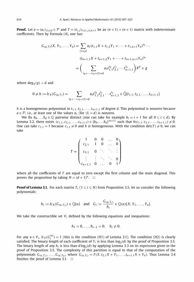
Proof. Let a = (aI )|I|�d ∈ P and T = (ti, j)1�i, j�n+1 be an (n + 1) × (n + 1) matrix with indeterminatecoefficients. Then by Formula (4), one has:

G(a,T )(X, Y1, . . . , Yn) =∑|I|�d

aI (t1,1 X + t1,2Y1 + · · · + t1,n+1Yn)i0 · · ·

(tn+1,1 X + tn+1,2Y1 + · · · + tn+1,n+1Yn)in

=( ∑

i0+···+in=|I|=d

aIti01,1ti1

2,1 · · · tinn+1,1

)Xd + g

where degX (g) < d and

0 �= h := lc X (G(a,T )) =∑

i0+···+in=|I|=d

aIti01,1ti1

2,1 · · · tinn+1,1 ∈ Q[t1,1, t2,1, . . . , tn+1,1]

h is a homogeneous polynomial in t1,1, t2,1, . . . , tn+1,1 of degree d. This polynomial is nonzero becausea ∈ P , i.e., at least one of the values aI (for |I| = d) is nonzero.

We fix b0, . . .bd ∈ Q pairwise distinct (one can take for example bi = i + 1 for all 0 � i � d). ByLemma 3.2, there exists (c1,1, c2,1, . . . , cn+1,1) ∈ {b0, . . .bd}(n+1) such that h(c1,1, c2,1, . . . , cn+1,1) �= 0.One can take c1,1 = 1 because c1,1 �= 0 and h is homogeneous. With the condition det(T ) �= 0, we cantake

T =

⎛⎜⎜⎜⎜⎜⎝

1 0 0 . . . 0c2,1 1 0 . . . 0

c3,1 0. . .

. . ....

......

. . .. . . 0

cn+1,1 0 . . . 0 1

⎞⎟⎟⎟⎟⎟⎠

where all the coefficients of T are equal to zero except the first column and the main diagonal. Thisproves the proposition by taking N = (d + 1)n . �Proof of Lemma 3.1. For each matrix Ti (1 � i � N) from Proposition 3.5, let us consider the followingpolynomials:

hi := lc X (G(u,Ti)) ∈ Q[u] and Gi := G(u,Ti)

hi∈ Q(u)[X, Y1, . . . , Yn].

We take the constructible set V i defined by the following equations and inequations:

h1 = 0, . . . ,hi−1 = 0, hi �= 0.

For any a ∈ V i , lc X (G(a)i ) = 1 (this is the condition (H1) of Lemma 2.1). The condition (H2) is clearly

satisfied. The binary length of each coefficient of Ti is less than log2(d) by the proof of Proposition 3.5.The binary length of any hi is less than d log2(d) by applying Lemma 3.3 on its expression given in theproof of Proposition 3.5. The complexity of this partition is equal to that of the computation of thepolynomials G(u,T1), . . . , G(u,T N ) where G(u,Ti) = F (X, t2,1 X + Y1, . . . , tn+1,1 X + Yn). Thus Lemma 3.4finishes the proof of Lemma 3.1. �


3.2. Applying Hensel’s lemma

In this section, we fix a couple (V , G) from Lemma 3.1. We know that for any a ∈ V , the polyno-mial G(a) ∈ Q[X, Y1, . . . , Yn] satisfies the conditions (H1) and (H2) of Lemma 2.1. Let us write G as inSection 2.1 in the form:

G = Xd +∑

0�|I|�d,0�i<d

vi,I X i Y I = G0 +∑

1�|I|�d

G I Y I

according to the bounds of Lemma 3.1 where vi,I ∈ Q(u). Let k = (k1, . . . ,ks) ∈ Ns be an orderedpartition of d, i.e., d = k1 + · · · + ks , k1 � · · · � ks � 1, we associate to this ordered partition a subsetUk of V defined by:

Definition 3.6. Uk is the set of values a ∈ V of the parameters such that the polynomial G(a) fulfillsthe following condition:

• (H3): There exist monic polynomials G(1)0 , . . . , G(s)

0 ∈ Q[X] such that

G(a)0 = G(1)

0 · · · G(s)0 and deg

(G( j)

0

) = k j for all 1 � j � s

and by application of Lemma 2.1 one gets a decomposition of G(a) in Q[X, Y1, . . . , Yn]. In otherwords, the ordinary power series G(a)

1 , . . . , G(a)s given by Lemma 2.1 are in fact in Q[X, Y1, . . . , Yn].

The latter condition will be called the termination condition.

Let us write the rational functions vi,I ∈ Q(u) (i.e., the coefficients of G) in the form:

vi,I = wi,I

hwhere h, wi,I ∈ Q[u]

and h(a) �= 0 for all a ∈ V (see the proof of Lemma 3.1). Then the condition G(a)0 = G(1)

0 · · · G(s)0 of

Definition 3.6 is equivalent to the following equalities:

w(a)i,0 = h(a)

∑0=l0�l1�···�ls=i

∏1�m�s

α(m)

lm−lm−1, 0 � i < d (5)

where α( j)k j

= 1 for all 1 � j � s and the α( j)i are the coefficients of G( j)

0 (as in Section 2.1). The follow-

ing lemma and theorem prove an equivalent condition to the termination condition of Definition 3.6.

Lemma 3.7. Let I be a multi-index such that |I| > d. Then G( j)I = 0 for all 1 � j � s if and only if H I = 0

where G( j)I are defined in Lemma 2.1 and H I is given by Formula (2) of Remark 2.2.

Proof. For |I| > d, we have G I = 0 because degY (G) � d by Lemma 3.1. Then H I = 0 if and only if thesecond member bI of the linear system Bx = bI of Remark 2.2 is zero. This is equivalent to that thesystem has 0 as its unique solution. This proves the lemma. �Theorem 3.8. The termination condition of Definition 3.6 is equivalent to the following equalities:

H I = 0, d < |I| � sd.


Proof. The termination condition is equivalent to the fact that degY (G j) � d for all 1 � j � s. This is

equivalent to G( j)I = 0 for all 1 � j � s and |I| > d. By Lemma 3.7, these conditions are equivalent to

that H I = 0 for all |I| > d. It remains to prove that it is equivalent to H I = 0 just for d < |I| � sd. Weprove it just for the case s = 2, the general case is analogous. By Remark 2.2, we have:

H I =∑

1�| J |<|I|G(1)

J G(2)I− J .

One has to prove that H I = 0 for all d < |I| � 2d implies H I = 0 for all |I| > d. We suppose thatH I = 0 for all d < |I| � 2d, then Lemma 3.7 ensures that G(1)

I = G(2)I = 0 for all d < |I| � 2d. Let us

prove by induction on t that H I = 0 for |I| = d + t and for all t � d + 1:

• For t = d + 1 (i.e., |I| = 2d + 1). We decompose H I into two sums as follows:

H I =∑

1�| J |�d

G(1)J G(2)

I− J +∑

d<| J |�2d

G(1)J G(2)

I− J .

For d < | J | � 2d, G(1)J = 0 then the second member is zero and for 1 � | J | � d, we get d <

|I − J | � 2d and G(2)I− J = 0 and then the first sum is zero. Thus H I = 0.

• We suppose that H I = 0 for d < |I| � d + t and t � d + 1. Then for |I| = d + t + 1, we have:

H I =∑

1�| J |�d

G(1)J G(2)

I− J +∑

d<| J |�d+t

G(1)J G(2)

I− J .

For d < | J | � d + t , G(1)J = 0 (by the hypothesis of the induction) and for 1 � | J | � d, we get

d < |I − J | � d + t and G(2)I− J = 0. Thus H I = 0. �

Remark 3.9. By Remark 2.2, each H I depends only of the polynomials G(1)J , . . . , G(s)

J for all multi-index

J such that | J | < |I|. We replace the coefficients of the polynomials G(1)J , . . . , G(s)

J (for all | J | < |I|) inthe new termination condition of Theorem 3.8 by their expressions given by Theorem 2.4. Then thecoefficients of H I are rational functions in the variables α

( j)i (which represent the coefficients of G( j)

0 )

and the parameters u, i.e., H I ∈ Q(α( j)i , u)[X]. Thus the termination condition is equivalent to certain

polynomial equalities in the form:

Q (I)t = 0, d < |I| � sd, � t � d − 2 (6)

where Q (I)t ∈ Q[α( j)

i , u].

Lemma 3.10. For any d < |I| � sd, 0 � t � d − 2, one has the following bounds:

⎧⎨⎩

degα

( j)i

(Q (I)

t

)� 2

(|I| − 1)(d − 1)(s − 1) � 2d4,

degu

(Q (I)

t

)� 2

(|I| − 1)(s − 1) � 2d3.

The binary length of Q (I)t is less than

4d log2 d + 2(|I| − 1

)(d − 1)(s − 1) � 6d4 log2 d.


Proof. (Case s = 2)

Q (I)t =

∑1�| J |<|I|,0�l�t

P (1, J )l P (2,I− J )

t−l .

By the bounds of Theorem 2.4, we get

degα

( j)i

(Q (I)

t

)�

(2| J | − 1

)(d − 1) + (

2|I − J | − 1)(d − 1) = 2

(|I| − 1)(d − 1),

degvi,I

(Q (I)

t

)�

(2| J | − 1

) + (2|I − J | − 1

) = 2(|I| − 1

).

Or by Lemma 3.1, degu(G) = 1 (and then degu(vi,I ) = 1). Thus degu(Q (I)t ) � 2(|I| − 1). By Lemma 3.3,

the binary length of Q (I)t is the maximum of the binary lengths of the terms P (1, J )

l P (2,I− J )t−l of its

formula above. Then by Lemma 3.3, Theorem 2.4 and Lemma 3.1 (L � d log2 d), the binary length ofQ (I)

t is bounded by:

maxl, J

{2L + (

2| J | − 1)(d − 1) + 2L + (

2|I − J | − 1)(d − 1)

}

� 4L + 2(|I| − 1

)(d − 1) � 4d log2 d + 2

(|I| − 1)(d − 1).

The final bounds are given using the fact that s � d. �Corollary 3.11. Let k = (k1, . . . ,ks) be an ordered partition of d where s � 2. Then the set Uk is the Q-realization in V of the following quantified formula:

∃α( j)i , 1 � j � s, 0 � i < k j which satisfy (5) and (6). (7)

The free variables of this formula are the parameters u.

Proof. By Definition 3.6, Theorem 3.8 and Remark 3.9. �Corollary 3.12. The number of equations in Formula (7) is

(d − 1)

((n + sd

n

)−

(n + d

n

))+ d � dO (n).

The number of its quantifiers is equal to d, the degrees of its equations w.r.t. α( j)i (resp. u) do not exceed 2d4

(resp. 2d3). The binary lengths of its equations are less than 6d4 log2 d.

Proof. The number of equations is done by the fact that the number of coefficients of a multivariatepolynomial with n variables of degree not exceeding d is

(n+dn

)� (d + 1)n . The other bounds are the

same bounds of Lemma 3.10. �Lemma 3.13. Let k be an ordered partition of d, then Uk is a constructible set defined by the following freequantifier formula:

∨1�i�α

( ∧1� j�β

(Pi, j = 0) ∧ (Ri �= 0)

)


where α,β � dO (nrd2) . For any 1 � i � α and 1 � j � β , the polynomials P i, j, Ri ∈ Q[u1, . . . , ur] satisfy thefollowing bounds:

• The binary length and the degree of P i, j w.r.t. u are less than dO (nrd2).

• The binary length and the degree of Ri w.r.t. u are less than dO (nd).

The computation of this formula is done by dO (nr2d3) binary operations.

Proof. By application of the quantifier elimination algorithm of Chistov–Grigoriev [5] (see Section 2.2)on Formula (7) which defines Uk (Corollary 3.11) taking into account the bounds given in Corol-lary 3.12. �Remark 3.14. The constructible sets Uk (where the k’s are the ordered partitions of d) do not forma partition of V and for any a ∈ Uk , the decomposition G(a) = G(a)

1 · · · G(a)s given by Hensel’s lemma is

not necessary an absolute factorization of G(a) .

To get a partition of V into constructible sets and an absolute factorization of G(a) uniformly ineach of them (i.e., PAFs of G), we introduce the following definition:

Definition 3.15. One says that an ordered partition k′ = (k′1, . . . ,k′

p) of d is finer than another orderedpartition k = (k1, . . . ,ks) of d if for any 1 � l � s, kl = k′

il+ k′

il+1 · · · + k′il+1−1 for certain 1 � i1 < · · · <

is � p.

Proposition 3.16. If k′ is finer than k then Uk′ ⊂ Uk.

Proof. By Definition 3.6. �Lemma 3.17. Let pt(d) be the set of all ordered partitions of an integer d. The cardinal of pt(d) does not exceeddd+1 .

Proof. The cardinal of pt(d) is given by

1 +∑

2�s�d

(d − 1 + s − 1

s

)� 1 +

∑2�s�d

(d − 1)s � 1 + (d − 1)d−1 − 1

d − 2(d − 1)2 � dd+1. �

Lemma 3.18. For each couple (V , G) of Lemma 3.1, the constructible sets Uk = Uk \ ⋃k′ �=k Uk′ ( for all k ∈

pt(d)) form a partition of V where the union ranges over all the ordered partitions k′ of d being finer than k.For each set Uk, there exist polynomials G1, . . . , Gs ∈ Q(C1, . . . , Cd, u)[X, Y1, . . . , Yn] where C1, . . . , Cd arenew variables. These polynomials satisfy the following properties:

• For any a ∈ Uk, there exists (c1, . . . , cd) ∈ Qd a solution of the algebraic system defined by Formulas (5)and (6) such that the denominators of the coefficients of G1, . . . , Gs do not vanish on (c1, . . . , cd,a) andthe absolute factorization of G(a) ∈ Q[X, Y1, . . . , Yn] is given by:

G(a) =∏

1� j�s

G(c1,...,cd,a)

j where G(c1,...,cd,a)

j is absolutely irreducible.

• For any 1 � j � s, degC1,...,Cd(G j) � 2d4 , degu(G j) � 2d3 , degX (G j) � d, degY (G j) � d. The binary

length of G j is less than 6d4 log2 d.


Proof. For each k ∈ pt(d), the polynomials G1, . . . , Gs are given by Hensel’s lemma (Lemma 2.1) andTheorem 2.4 with rational function coefficients in the parameters u and the indeterminate coefficientsC1, . . . , Cd of G(1)

0 , . . . , G(s)0 . The degrees and binary lengths are deduced from Corollary 3.12. �

3.3. Reduction to solving zero-dimensional parametric polynomial systems

For each couple (V , G) of Lemma 3.1, Lemma 3.18 gives a kind of PAFs for the parametric multi-variate polynomial G ∈ Q(u)[X, Y1, . . . , Yn]. To get PAFs of the original parametric multivariate poly-nomial F , we will replace the variables C1, . . . , Cd of Lemma 3.18 by only one variable C and wewill show how to pass from the absolute factorization of G(a) (given by Lemma 3.18) to that of F (a)

uniformly in the values a of the parameters.The following theorem is the main result of the paper, it is similar to Theorem 1.5 but with bounds

and complexity analysis.

Theorem 3.19. There is an algorithm which computes at most dO (nr2d2) PAFs (W , φ, G1, . . . , Gs) of F suchthat the constructible sets W form a partition of the parameters space P . Moreover, the following bounds hold:

• The degrees of the equations and inequations that define a constructible set W are equal to dO (nr2d2) . Theirbinary lengths are equal to dO (nr2d2) .

• For any 1 � j � s, the degrees of φ and G j w.r.t. C (resp. u) are equal to dO (d) (resp. dO (rd2)). Their binary

lengths are equal to dO (rd2) .

The number of arithmetic operations of the algorithm is dO (nr2d3) and its binary complexity is dO (nr2d3) .

Proof. We fix a constructible set Uk ⊂ V given by Lemma 3.18 and we consider the parametricpolynomial system S which is defined by Eqs. (5) and (6). The parameters of S are the variablesu = (u1, . . . , ur), its unknowns are the variables C1, . . . , Cd which replace the variables α

( j)i in these

equations. For any a ∈ Uk , the system S(a) (obtained after specialization of the parameters u by a)admits a finite number of solutions which correspond to the permutations of the factors of G(a)

0 (seeDefinition 3.6). Namely, there is a bijective correspondence between the solutions of S(a) and thepermutations of the factors of G(a)

0 .By applying the algorithm of Section 2.3 to the zero-dimensional parametric polynomial system S ,

we get a partition of Uk into dO (r2d2) constructible sets W such that for each set W , the algorithmcomputes polynomials φ,ψ1, . . . ,ψd ∈ Q(u)[C] which satisfy the following properties:

• All rational functions coefficients of φ,ψ1, . . . ,ψd are well-defined on W .• For any a ∈ W and for any solution (c1, . . . , cd) ∈ Qd of the system S(a) , there exists c ∈ Q, a root

of φ(a) ∈ Q[C] such that ci = ψ(a)i (c), ∀i = 1, . . . ,d.

• The degrees of the equations and inequations that define W are equal to dO (r2d2) . Their binarylengths are less than dO (r2d2) .

• For any 1 � j � d, the degrees of φ and ψ j w.r.t. C (resp. u) are equal to dO (d) (resp. dO (rd2)).

Their binary lengths are equal to dO (rd2) .

This partition is done by dO (r2d2) operations in Q. Its binary complexity is dO (r2d2) . The above boundsare done by taking into account those of the system S which are given in Corollary 3.12. We fixnow a set W and we replace the expressions Ci = ψi(C), ∀i = 1, . . . ,d, in the coefficients of thepolynomials G1, . . . , Gs ∈ Q(C1, . . . , Cd, u)[X, Y1, . . . , Yn] of Lemma 3.18. One gets new polynomials


G j ∈ Q(C, u)[X, Y1, . . . , Yn] (we retain the same names). For any a ∈ W , there exists c ∈ Q, a root ofφ(a) ∈ Q[C] such that the absolute factorization of G(a) is given by:

G(a) =∏

1� j�s

G(c,a)j , G(c,a)

j is absolutely irreducible.

This means that the tuples (W , φ, G1, . . . , Gs) are now PAFs of G .To pass from the absolute factorization of G(a) to that of F (a) , one has to return to the form of the

polynomial G which is given by Formula (4) and the proof of Lemma 3.1. This can be done by thecomputation of the inverse of the matrix T which defines G .

The degrees of the equations and inequations that define the elements of the partition is themaximum of those of V (Lemma 3.1), Uk (Lemma 3.13) and W (from above).

It remains to count the number of elements of the partition of the parameters space P and toestimate the total complexity of the algorithm. First, the number of sets V is � (d + 1)n (Lemma 3.1),that of the sets Uk for k ∈ pt(d) is � dd+1 (Lemma 3.17) and that of the sets W is � dO (r2d2) (fromabove). Therefore the total number of the elements of the partition of P is � (d + 1)n × dd+1 ×dO (r2d2) � dO (n+r2d2) .

Second, for any multi-index I , the computation of the coefficients of the polynomials G(1)I , . . . , G(s)

I(i.e., the resolution of the linear system Bx = bI of Remark 2.2) costs O (d2.376) operations in Q (seee.g. [10]). To construct the equations of Formula (7) which defines Uk , it was necessary to computeall the polynomials G(1)

I , . . . , G(s)I for all 1 � |I| � sd. The complexity of this computation is given by(n+sd

n

)O (d2.376) � dO (n) . Since the number of ordered partitions k of d is � d(d+1) (by Lemma 3.17),

then the complexity of the construction of all the sets Uk is dd+1 ×dO (n) ×dO (nr2d3) � dO (nr2d3) opera-tions in Q (the third factor is the complexity bound in Lemma 3.13). Its binary complexity is dO (nr2d3) .By taking also into account the complexity of computing the sets V (Lemma 3.1) and that of the setsW (from above), we get the total complexity of the algorithm. �3.4. The general case

When the coefficients of F ∈ Q[u][X0, . . . , Xn] are polynomials in the parameters u of degrees notexceeding an integer δ and binary lengths less than an integer L, we still can follow the steps ofthe algorithm of Section 3 to compute PAFs of F . Theorem 3.19 is still valid but the bounds on thedegrees of the output polynomials and the complexity of the algorithm are changed by adding newfactors of powers of δ and L as follows:

• The degrees of the equations and inequations that define each element of the partition of theparameters space are equal to δO (r2)dO (nr2d2) . Their binary lengths are equal to LδO (r2)dO (nr2d2) .

• For any 1 � j � s, the degrees of φ and G j w.r.t. C (resp. u) are equal to δdO (d) (resp. δO (r)dO (rd2)).

Their binary lengths are equal to LδO (r)dO (rd2) .

The number of arithmetic operations of the algorithm is δO (r2)dO (nr2d3) and its binary complexity isLδO (r2)dO (nr2d3) .

When the parameters u1, . . . , ur are algebraically dependent over Q, i.e., the parameters space Pis equal to a certain constructible set U , then the algorithm of Theorem 3.19 returns a partition ofP into a finite number of constructible sets W = W ∩ U such that the tuples (W , φ, G1, . . . , Gs) arePAFs of F .

References

[1] A. Ayad, Complexity bound for the absolute factorization of parametric polynomials, Zap. Nauchn. Sem. S.-Peterburg. Otdel.Mat. Inst. Steklov. (POMI) 316 (2004) 5–29, Teor. Slozhn. Vychisl. 9 (224) (2004) 5–29, translation in J. Math. Sci. (N.Y.) 134(2006) 2325–2339.


[2] A. Ayad, Complexité de la résolution des systèmes algébriques paramétriques, PhD thesis, University of Rennes 1, France,2006.

[3] A. Ayad, An algorithm for solving zero-dimensional parametric systems of polynomial homogeneous equations, submittedfor publication.

[4] S. Basu, R. Pollack, M.-F. Roy, Algorithms in Real Algebraic Geometry, Springer, New York, 2003.[5] A. Chistov, D. Grigoriev, Complexity of quantifier elimination in the theory of algebraically closed fields, in: Lecture Notes

in Comput. Sci., vol. 176, Springer, 1984, pp. 17–31.[6] A.L. Chistov, Algorithm of polynomial complexity for factoring polynomials and finding the components of varieties in

subexponential time, J. Sov. Math. 34 (1986) 1838–1882.[7] D. Grigoriev, Factorization of polynomials over a finite field and the solution of systems of algebraic equations, J. Sov.

Math. 34 (1986) 1762–1803.[8] D. Grigoriev, N. Vorobjov, Bounds on numbers of vectors of multiplicities for polynomials which are easy to compute, in:

Proc. ACM Intern. Conf. Symbolic and Algebraic Computations, St. Andrews, Scotland, 2000, pp. 137–145.[9] A. Montes, A new algorithm for discussing Gröbner basis with parameters, J. Symbolic Comput. 33 (2002) 183–208.

[10] J. von zur Gathen, J. Gerhard, Modern Computer Algebra, second ed., Cambridge Univ. Press, 2003.[11] H. Zassenhaus, On Hensel factorization, J. Number Theory 1 (1969) 291–311.

on factoring parametric multivariate polynomials

Documents