on-farm cost os f reducing environmental...

O N - F A R M C O S T S O F R E D U C I N G E N V I R O N M E N T A L D E G R A D A T I O N U N D E R RISK

David Letson Parveen P. Setia*

Resumen: Los productores agrícolas responden a las regulaciones ambientales ajustando sus prácticas de producción a través de la minimización de sus pérdidas de ingreso esperado. Esencialmente, el costo de regular el medio agrícola está determinado por los ajustes que se tienen que hacer a nivel de productor. Nuestra estructura de simulación a este nivel evalúa los efectos económicos y ambientales de restricciones hipotéticas en el uso de pesticidas en un contexto donde continúan los esfuerzos de conservación del suelo.

Abstract: Farmers respond to environmental regulations by adjusting production practices so as to comply while minimizing their loss in expected income. Ultimately the cost of agro-environmental regulation is determined by farm-level adjustments. Our farm-level simulation framework assesses economic and environmental impacts of hypothetical pesticide restrictions in the context of continuing soil conservation efforts.

1. Introduction

Nonpoint source pollution efforts in U.S. agricultural policy historically have emphasized voluntary control of soil erosion and surface runoff. Not all water quality problems fit neatly into this focus,

* The authors are economists with the Natural Resources and the Environment Division, Economic Research Service, U.S. Department of Agriculture. The views expressed are those of the authors and do not represent policies or views of the United States Department of Agriculture. We would like to thank Steve Crutchfield, Wen Huang, and Marc Ribaudo for their comments. Discussions with R.R. Venkataraman were especially helpful. The usual caveat applies.

EEco, 9, 2, 1994 163

164 E S T U D I O S E C O N Ó M I C O S

however. The detection of agricultural chemicals in groundwater has raised much concern, for example. In their nationwide well survey, the U . S . Environmental Protection Agency reports the detection of pesticide residues in about ten percent of the community wells and four percent of the private wells surveyed ( U S E P A 1991; U S E P A 1994). With the onset of additional pollution concerns in agriculture comes the need for analytical tools to assess the costs of controlling the multidimensional problem.

The cost of agricultural nonpoint source pollution control is difficult to determine when (1) control of one pollutant can result in the release of others, or (2) instead of being controlled, pollutants can be shifted to different environmental media. In addition to limiting the burden on farmers, policy makers also must contend with possibly opposing environmental goals, such as soil conservation and the reduction of pesticide applications. The physical linkage of surface and groundwater systems and air quality provides a setting for another example of conflicting environmental goals, since it suggests that policy analysis needs to address surface and ground water quality, and air quality as well. Many researchers have considered restriction on pesticides (Lichtenberg et al., 1988; Anderson et al, 1985), sedimentation (Kramer et al., 1983; Braden et al, 1989), or nutrients (Park and Shab-man, 1982; Johnson et al., 1991), but without attempting to limit such intermedia effects.

Another complication in costing environmental control in agriculture is that regulatory burden on farmers can come in the form of increased risk bearing. New restrictions on land and chemical use would create additional variability in revenue and input supplies, as well as new input costs. Uncertainty in farm income and farmer's attitudes toward risk add to the cost of alternative production practices, or management systems, needed to meet environmental goals (Collins and Headley, 1983; Ervin, 1982; and Kramer et al., 1983). Usually, researchers have given joint rather than separate consideration to farmers' attitudes toward variation in income and soil loss.

This paper captures these important elements of the agricultural water quality problem. Because the burden of new pesticide regulations depends on farmers' ability to substitute out of more costly inputs and less profitable outputs (Kramer et al., 1983), we adopt a farm-level analytical framework. We consider farm-level decisions with a quad-

REDUCING ENVIRONMENTAL DEGRADATION 165

ratic programming model of a typical, 121.4 hectare (300 acre) cash grain farm in the U.S. western cornbelt (i.e., Missouri, Illinois and Iowa). The model is comprehensive in limiting soil loss and pesticide loadings to the air, surface runoff, and leachate below the root zone. To consider risk, we use a stochastic simulator to generate separate probabilistic parameters for soil loss and net income that reflect the added production risk of regulation. These parameters are input for the quadratic programming model.

We use the quadratic programming model to consider two sets of issues. First, how do the level of risk aversion and the probability of meeting the soil loss goals influence farmer income and the choice of management systems? Second, how will the farmer respond to conservation and environmental regulations? Here we relate farmer income and the choice of management systems to restrictions on soil loss and pesticide loadings. By assessing the farmer's possible response to risk and resource use restrictions, we hope to gain a clearer picture of the cost of managing multi-dimensional environmental problems caused by agriculture.

2. Analytical Framework

2.1. Overview

Policy makers want to achieve environmental goals while minimizing the regulatory burden on the farming community. More stringent regulation of inputs and production practices generally, but not always, wil l have a detrimental effect on farming profitability; the magnitude of that effect, however, is a matter of contentious debate. What is needed is a rigorous assessment of the profitability of alternative management systems. A n extensive literature exists on the comparative economics of alternative agricultural production systems (e.g., Shortle and Miranowski, 1987; and Taylor and Frohberg, 1977; for a review, see Fox et al., 1991). Our contribution is our separate treatment of different types of risk and our control of intermedia pollutant transfers.

The policy assessment should faithfully represent the productive capabilities of alternative management systems. In most cases, risk should be considered, because of randomness in prices, yields, and


resource availability, and because numerous studies have demonstrated that farmers are risk averse (e.g., Binswanger, 1980; Dillon and Scan-dizzo, 1978). The farmer often is willing to sacrifice some income, on average, for security and wil l select a portfolio of enterprises. Farmers' regulatory burden ultimately depends on their flexibility in portfolio management, substituting out of regulated inputs and into more profitable outputs (Kramer et al., 1983). The policy assessment should also consider the transport of pollutants to environmental media and the chemical transformations the pollutants undergo during transport. To inform policy makers on the merits of alternative strategies, researchers must appropriately characterize environmental and farm production systems so that hypothetical policy changes can be accurately transformed into economic and environmental outcomes.

In our research we have used a simulation framework having two components. The first is the Stochastic Soil Conservation Economics model ( S S O I L E C ) , which is a stochastic, dynamic farm production simulator developed by the University of Illinois Department of Agricultural Economics (Setia and Johnson, 1988). S S O I L E C used site-specific physical and economic data to generate parameters for the second component of the simulation, a quadratic programming model ( Q P ) . S S O I L E C yielded means and covariances for net income and soil loss for each management system. The Q P determined optimal combinations of management systems under various regulatory scenarios (i.e., soil loss and pesticide restrictions). An U S E P A study (Donigian et al., 1986) provided pesticides fate and transport data for the Q P . The Q P maximizes net income under risk, subject to desired reductions in soil loss and potential pesticide loadings to air, surface runoff, and leachate below the root zone.

2.2. Simulated and Historical Data

We selected the 24 management systems most prevalent in the study area: two crop rotations (continuous corn and corn-soybeans), three tillage systems (conventional tillage, reduced tillage, no-till), and four mechanical control practices (vertical plowing, contouring, stripcropping, and contouring and terracing). A stochastic simulator ( S S O I L E C ) calculated the impact of sheet and rill erosion on soil productivity and production costs. It consists of four basic relationships: the universal soil loss equation

R E D U C I N G E N V I R O N M E N T A L D E G R A D A T I O N 167

( U S L E ) , discounted net returns, and the relationships between crop yield and soil loss and between production costs and soil loss, S S O I L E C linked physical and economic information for each management system over the 25-year planning horizon to capture the intertemporal nature of soil loss.

To simulate effects of soil erosion on net returns over time and under different soil management systems, we gathered field data from four experimental farms operated by the University of Illinois' Department of Agronomy, which were reviewed and approved by the U.S. Department of Agriculture's Extension Service in Illinois. Our data describe a typical farm in the U .S . western cornbelt and include the following factors: annual production costs for each system, specific to this region and the soil types; U S L E factors; production cost and crop yield adjustments for mechanical control practices; crop yield adjustments for tillage effects; crop residue production; 30-year (1957-1986) historical joint probability distributions1 (for commodity prices, crop yields, and weather); and confidence level parameters and safety income level (Baumol, 1963; Boussard and Petit, 1967). These data represent typical values for the region's farms. For a detailed description of S S O I L E C and our data sources, see Setia and Johnson (1988) and Venkataraman (1988). S S O I L E C calculated annualized net returns for each management system with a real discount rate of 8 percent and 25-year planning horizon. 2

There are at least four possible sources of uncertainty in our model: crop yields, weather (i.e., the U S L E /^-factor, a measure of rainfall as it affects erosion), crop prices and production costs. Reasonable assumptions about these sources of variation allowed us to simplify our modeling framework. First, we assume production costs to be constant and known at the time of planting. Second, we assume no correlation between crop yields and prices, since the latter are determined on the world level, while yields are site specific. Third, we assume no correla-

1 To correct for an upward bias due to inflation and technological change, the varíate difference method was used to detrend the data. This method allows the mathematically predictable expected components of the data to be removed and the variances and co variances calculated on the residual random component of the data (Tintner, 1940). This approach assumes that predictable components of the data do not contribute to risk.

2 We used a range of discount rates, from 4 to 10 percent. We do not report here the results from discount rates other than 8 percent, because the change influenced income levels but not our principle interest, the pattern of management systems adopted.


tion between crop yields and the /?-factor. While rainfall often wi l l not affect yields because of the time of year it is delivered, it almost certainly wi l l affect soil loss considerably in the U S L E (Setia and Johnston, 1988).

One notable complication did arise: the stochastic nature of weather, crop prices, and crop yields causes net returns to be random as well. Because the stochastic variables interrelate in a multiplicative manner (e.g., price * yield = gross returns), it is difficult to directly predict their effect on variability in net returns. Monte Carlo analysis overcame this prediction problem. We ran the simulator repeatedly by randomly sampling from the joint probability distributions of the stochastic variables (weather, crop yields, and crop prices), generating a distribution of outputs (net returns) reflecting conditions at the farm (Rubinstein, 1981; Setia and Johnson, 1988). Theoretically, an infinite number of observations needs to be generated by this method. However, we ceased our simulations after 700 runs when the results stabilized, i.e., additional observations did not influence mean and variance values.

Lastly, we were fortunate enough to find information about pesticide loadings that met our needs. A n essential part of this research was fate and transport information reliable and simple enough to be included in our Q P . The potential pesticide loadings to different environmental media (air, surface runoff, and leached below the root zone) for each management system were provided by an E P A pesticide fate and transport modeling analysis (Donigian etaL, 1986). This study used the physical process models P R Z M and AT123D to generate linear loading coefficients for nine pesticides and takes into account the effect of weather, pesticide and soil characteristics, tillage practices, and crops (Pesticide Root Zone Modeling System, Carsel 1986; Analytical Transient One-, Two-, Three-Dimensional Simulation of Waste Treatment in the Aquifer System, Yeh, 1986). P R Z M models pesticide mass loadings to leachate, runoff, and volatilization as a function of pesticide properties, meteorological conditions, soil and crop characteristics, tillage practices, and application rates. AT123D uses the P R Z M predictions of leachate loadings to model solute transport in aquifer systems, giving pesticide concentrations in groundwater. A detailed description of the analytical framework used to estimate the pesticide loadings coef-fients is given in Donigian et al. (1986).


2.3. Economic Optimization Model

Thus far we have assembled data and parameters to characterize production and environmental systems. What remains is our specification of the farmer's decision analysis. The farmer wi l l rank farm plans on the basis of their income distributions. Several alternatives exists for such a ranking. The most established decision theory in economics is expected utility theory, as developed by von Neuman and Morgenstern (1944). The conceptual appeal of this approach derives from its reliance on a set of behavioral axioms rather than a particular functional form. However, the theoretical generality of the expected utility approach comes at the expense of computational ease, particularly when looking at multiple risky assets. Anderson, Dillon, and Hardaker (1977) review the attempts to use the axioms of expected utility theory to elicit individual utility functions. A more practical approach is to assume a computationally convenient functional form, and mean-variance ( E V ) analysis as developed by Markowitz (1959) is one means for doing so. The E V approach assumes that the farmer's preferences among alternative farm plans are based on the expected value and variance of the income associated with those plans. For a more detailed discussion of expected utility theory and mean-variance analysis, see Hazell and Norton (1986) or Anderson, Dil lon, and Hardaker (1977).

We solve our E V model using Q P to analyze farm production decisions under various regulatory scenarios3 (see Robison and Brake (1979) for a review of E V model applications to agriculture). Farmers' regulatory burden depends on their ability to substitute out of regulated inputs and into more profitable outputs (Kramer et al., 1983). Our Q P allows the farmer to select the ex ante most profitable, fixed input/output combinations (i.e., management systems). Regulatory burden also depends on the farmer's risk preferences. Alternative management sys-

3 To use the EV model we assumed an exponential value function to approximate the farmer's utility function, which implies constant absolute risk aversion, and normally distributed earnings, which we confirmed for our simulations with the chi-square goodness of fit test (a = 0.025). In place of these two assumptions, we could have used a quadratic utility function but did not because of its diminishing marginal utility of income and increasing absolute risk aversion properties. These assumptions underlying EV make it less general than expected utility models, but also much easier to solve: maximizing our mean-variance objective function is equivalent to maximizing the expected value of the utility function (Freund, 1956).

170 ESTUDIOS ECONÓMICOS

tems require capital and specialized management skills; income risk posed by regulation and farmers' attitudes toward that risk influence adoption as they would any investment decision (Collins and Headley, 1983; Ervin, 1982; and Kramer et al, 1983).

The Q P has the following structure. In the objective function (1), discounted expected returns (y) are the difference between expected net income and the variance of net income, weighted by the risk aversion parameter (O). Ideally, the variance term should be based on the decision maker's subjective assessment of the relevant risks, although this has rarely been done (Lin et al., 1974, is an exception). Instead, we use our objective measure of variability and assume the farmer bases his/her plans on the mean and variance of a historical series of returns. For the atrazine ban simulation, the adjustment factor adj adjusts total expected returns for yield loss and increased input costs (Osteen and Kuchler, 1986); in all other runs of the model this factor was set to zero.

The first constraint (2) requires the total number of hectares planted in each land (i.e., soil characteristics) group (x) not to exceed available hectares (L"). The farm we consider is comprised of land groups in the same proportion as exists for the western cornbelt, according to the 1982 National Resources Inventory. We considered land groups Flanagan, Grundy, Tama, Clinton, Ridgeville, Drummer, and Fayette.

The second constraint (3) is the deterministic form of a chance constraint on soil loss. The probability of the expected soil loss exceeding the erosion limit (SLU) must be less than a. We convert the probabilistic soil loss constraint to deterministic form by changing a to D, the standardized normal value associated with an a probability that soil loss will not be greater than SLU (Chames and Cooper, 1959).4

Since D is positive for risk averse decision makers, the effect of risk in soil loss is to increase resource usage per unit of activity (Segarra et al., 1985). In our model, that means switching to less erosive management practices, but ones that also offer lower net income.

4 Some evidence suggests that rain fall, and thus soil loss, is log normally distributed (Wischmeier and Smith, 1978). Our assumption is that, with our large sample (700 samples of n = 30), the central limit theorem holds, so that the sample means are normally distributed.


The third constraint (4) restricts pesticide loadings to the environment.5 It requires that the sum of the number of hectares planted (x) times the potential pesticide loadings coefficients (PS) be less than a specified standard (PSU), for leaching below the root zone, surface runoff, and volatilization. The farmer chooses pesticides and management systems simultaneously and may use any pesticide with any system. However, the amount of a given pesticide used with a particular management system is fixed. In our simulated atrazine ban, we adjust the objective function for the increased input costs and diminished yields from using substitutes (Osteen and Kuchler, 1986). For the other policies pesticides enter the farmer's decisions through this constraint only. In all cases, the farmer must use more of the less effective substitutes to achieve the same effect and in doing so may increase pesticide loadings to the environment. If so, s/he may also have to shift to less chemical intensive management systems.

Lastly, the fourth constraint (5) requires non-negativity of the choice variables (x). The QP maximizes expected returns subject to constraints on land usage, soil loss, and pesticide loadings:

maximize y = X x * (R - ad] ) J m,x,p m,s,p v m, s Jm,s'

subject to

• 0 / 2 * X x c 2 x (1) m, m, s, p s, m, p r m, m, s in, s, p x '

^ V . , ^ ' (2)

for all land groups s € S

I x SL +D*[Z x a2 x ]i/2<SLu

m.p m,s,p m, .v L m,m,p s,m,p sm,m,s m,s,pJ s (3)

for all s G S

5 We restrict pesticide loadings, rather than applications, even though this would be difficult if not impossible to enforce in practice. We do so as a modeling expedient, assuming that in some settings (i.e. a small number of farmers in a clearly defined watershed) a regulator would be able infer application rates from our parameter values and simulation findings.


I x PS <PSU (4) m, s m, s, p m, e, p e,p v '

for all environmental media e e E and pesticides p e P

x >0 (5) m, s, p v 7

for all management systems me M,s e S and pe P. Where

adym v is the adjustment to expected net returns for the atrazine ban (= 0 when no atrazine ban),

D is a standardized normal value associated with an a probability, L u

s is upper bound on available land, PSm, e, p are pesticide loadings, PS" p are the upper bounds on pesticide loadings, Rm v is expected net income, SLnh s is the expected soil loss, SLU

S is the upper bound on soil loss, x t n s p is land planted, y is risk adjusted or expected net income, O is the Arrow-Pratt coefficient of absolute risk aversion, and <52 and a? are covariance matrices for income (r) and soil loss (s).

3. Results and Discussion

To assess the impact of possible pesticide restrictions, we investigated two sets of issues with the Q P . First, how are farm income and management system choices affected by the level of risk aversion toward income and by the probability of meeting the soil loss goals? Second, how do farm income and management system choices respond to soil loss and potential pesticide loadings restrictions?

To look at the two sets of issues we performed four simulations. In the first three simulations we accumulated, one by one, the land, soil loss, and pesticide constraints to see the additional net income and environmental effects of each. In other words, the three runs included the following constraints: land; land and soil loss; land, soil loss, and pesticides. In the fourth simulation we considered two different

REDUCING E N V I R O N M E N T A L DEGRADATION 173

kinds of pesticide restrictions. In the first (Status Quo), we restricted potential pesticide loadings to be no greater than what would occur without the soil loss constraint, while requiring those leached below the root zone to reduce by 20%; the objective was to reduce leaching in the context of soil conservation measures. The second scenario is a ban on atrazine, which induces substitution of other herbicides, such as cyanazine. The simulations illustrate some differences in farmers' responses to risk in income and soil loss; they also demonstrate some tradeoffs inherent in managing multi-dimensional agro-environmental problems.

3.1. Simulation One: Land Constraint Only

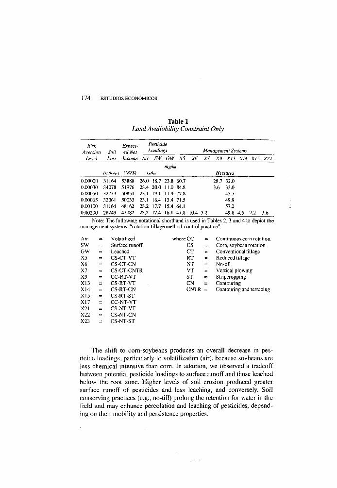
Table 1 shows how expected returns and the choice of management system vary as the level of risk aversion (O) increases.6 At higher levels of O, the farmer chooses a larger number of management systems, indicating the expected enterprise diversification to reduce variability of net income. Because the settings for this parameter are somewhat arbitrary, we selected a wide range of values to evaluate a broad range of possible farmer attitudes. Following Kramer et al. (1983), Tauer (1986), and Boggess and Ritchie (1988), we selected a range from 0 (risk neutral) to 0.002 (very high risk aversion).7 Expected net income varied by 20% over this range, confirming the breadth of our range of settings.

Management systems involving a corn-soybean rotation are preferred because of the higher expected value and lower variance of net income. However, these systems cause soil loss to be far greater than the tolerance level (6726 kg/ha/yr or 3 tons per acre per year ( T A Y ) )

or the national goal of 5 T A Y (11210 kg/ha/yr) because they incorporate the relatively more erosive crop, soybeans, in the rotation. While higher levels of risk aversion induce a shift from conventional to reduced tillage, conserving both soil and moisture and offsetting the increase in soil loss, the levels of soil loss remain far above tolerance levels.

6 These results may overstate the amount of diversification a single farmer would choose, because of the additional managerial expertise, machinery tooling requirements, and machinery transportation logistics required for each system. New systems might require some minimal acreage before they would become practical. At the regional level, however, production changes in the stated proportions are plausible.

7 A level of 0.0001 means that marginal utility decreases at a rate of .01 percent per dollar increase in returns, and the farmer is said to be risk averse because s/he derives less additional satisfaction from an additional dollar of income.


Table 1 Land Availability Constraint Only

Risk Aversion

Level Soil Loss

Expected Net Income

Pesticide Loadings Management Systems

Risk Aversion

Level Soil Loss

Expected Net Income Air SW GW X5 X6 X7 X9 X13 X14 X15 X21

(kx/haAtr) ('87$) mg/ha

kg/ha Hectares

0.00000 31164 53888 26.0 18.7 23.8 60.7 28.7 32.0 0.00030 34078 51976 23.4 20.0 11.0 84.8 3.6 33.0 0.00050 32733 50851 23.1 19.1 11.9 77.8 43.5 0.00065 32061 50033 23.1 18.4 13.4 71.5 49.9 0.00100 31164 48162 23.2 17.7 15.4 64.1 57.2 0.00200 28249 43082 23.2 17.4 16.1 47.8 10.4 3.2 49.8 4.5 2.2 3.6

Note: The following notational shorthand is used in Tables 2, 3 and 4 to depict the management systems: "rotation-tillage method-control practice".

Air = Volatilized where C C = Continuous corn rotation SW = Surface runoff CS = Corn, soybean rotation GW = Leached CT = Conventional tillage X5 = CS-CT-VT RT = Reduced tillage X6 = CS-CT-CN NT = No-till X7 = CS-CT-CNTR VT = Vertical plowing X9 = C C - R T - V T ST = Stripcropping X13 = CS-RT-VT CN = Contouring X14 = CS-RT-CN CNTR = Contouring and terracing X15 = CS-RT-ST X17 = C C - N T - V T X21 = CS-NT-VT X22 = CS-NT-CN X23 = CS-NT-ST

The shift to corn-soybeans produces an overall decrease in pes ticide loadings, particularly to volatilization (air), because soybeans are less chemical intensive than corn. In addition, we observed a tradeoff between potential pesticide loadings to surface runoff and those leached below the root zone. Higher levels of soil erosion produced greater surface runoff of pesticides and less leaching, and conversely. Soil conserving practices (e.g., no-till) prolong the retention for water in the field and may enhance percolation and leaching of pesticides, depending on their mobility and persistence properties.


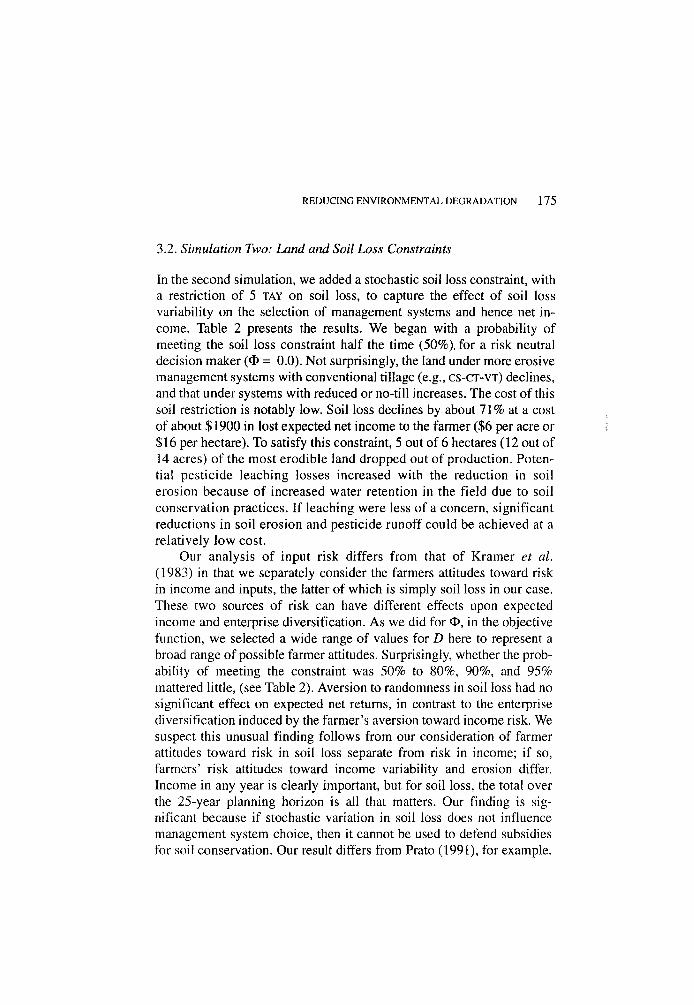
3.2. Simulation Two: Land and Soil Loss Constraints

In the second simulation, we added a stochastic soil loss constraint, with a restriction of 5 T A Y on soil loss, to capture the effect of soil loss variability on the selection of management systems and hence net income. Table 2 presents the results. We began with a probability of meeting the soil loss constraint half the time (50%), for a risk neutral decision maker (O = 0.0). Not surprisingly, the land under more erosive management systems with conventional tillage (e.g., C S - C T - V T ) declines, and that under systems with reduced or no-till increases. The cost of this soil restriction is notably low. Soil loss declines by about 71% at a cost of about $1900 in lost expected net income to the farmer ($6 per acre or $16 per hectare). To satisfy this constraint, 5 out of 6 hectares (12 out of 14 acres) of the most erodible land dropped out of production. Potential pesticide leaching losses increased with the reduction in soil erosion because of increased water retention in the field due to soil conservation practices. If leaching were less of a concern, significant reductions in soil erosion and pesticide runoff could be achieved at a relatively low cost.

Our analysis of input risk differs from that of Kramer et al. (1983) in that we separately consider the farmers attitudes toward risk in income and inputs, the latter of which is simply soil loss in our case. These two sources of risk can have different effects upon expected income and enterprise diversification. As we did for O, in the objective function, we selected a wide range of values for D here to represent a broad range of possible farmer attitudes. Surprisingly, whether the probability of meeting the constraint was 50% to 80%, 90%, and 95% mattered little, (see Table 2). Aversion to randomness in soil loss had no significant effect on expected net returns, in contrast to the enterprise diversification induced by the farmer's aversion toward income risk. We suspect this unusual finding follows from our consideration of farmer attitudes toward risk in soil loss separate from risk in income; if so, farmers' risk attitudes toward income variability and erosion differ. Income in any year is clearly important, but for soil loss, the total over the 25-year planning horizon is all that matters. Our finding is significant because if stochastic variation in soil loss does not influence management system choice, then it cannot be used to defend subsidies for soil conservation. Our result differs from Prato (1991), for example.


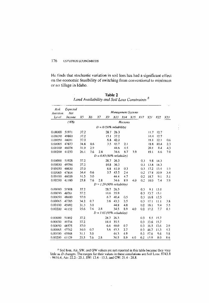
He finds that stochastic variation in soil loss has had a significant effect on the economic feasibility of switching from conventional to minimum or no tillage in Idaho.

Table 2 Land Availability and Soil Loss Constraints 8

Risk Expected Aversion Net Management Systems

Level Income X5 X6 X7 X9 XI3 X14 X15 X17 X2J X22 X23

cm) Hectares

D = 0 (50% reliability)

0.00000 51971 37.2 28.7 26.3 11.7 12.7 0.00030 49860 37.2 15.1 37.2 14.4 12.7 0.00050 48691 37.0 6.8 42.0 18.1 12.1 0.6 0.00065 47873 34.8 0.6 3.5 43.7 2.1 18.8 10.4 2.3 0.00100 46078 31.9 2.9 44.6 4.5 20.1 8.4 4.3 0.00200 41233 26.1 7.6 2.8 34.6 8.7 3.9 19.1 6.6 7.0

D = 0.85 (80% reliability)

0.00000 51928 37.2 28.7 26.3 0.3 9.8 14.3 0.00030 49794 37.2 14.8 36.3 0.3 13.8 14.3 0.00050 48630 37.0 6.8 41.0 0.3 0.3 17.2 13.4 1.9 0.00065 47814 34.4 0.6 3.5 43.5 2.4 0.2 17,8 10.9 3.4 0.00100 46020 31.5 3.0 44.4 4.7 0.2 18.7 9.1 5.1 0.00200 41180 25.8 7.6 2.8 34.6 8.9 4.0 0.2 18.0 7.4 7.9

D = J.29 (90% reliability)

0.00000 51908 37.2 28.7 26.3 0.3 9.1 15.1 0.00030 49761 37.2 14.6 35.9 0.3 13.7 15.1 0.00050 48600 37.0 6.7 40.4 0.5 0.3 16.8 12.5 0.00065 47785 34.2 0.7 3.6 43.3 2.5 0.3 17.1 11.1 3.8 0.00100 45992 31.3 3.0 44.8 4.8 0.2 18.1 9.4 5.5 0.00200 41152 25.6 7.6 2.8 34.5 8.9 4.0 0.2 17.2 7.7 8.3

D = 1.65 (95% reliability)

0.00000 51892 37.2 28.7 26.3 0.3 8.5 15.7 0.00030 49734 37.2 14.4 35.5 0.3 13.6 15.7 0.00050 48575 37.0 6.6 40.0 0.7 0.3 16.5 12.6 2,9 0.00065 47762 34.0 0.7 3.6 43.3 2.7 0.3 16.7 11.3 4.2 0.00100 45968 31.1 3.0 44.3 4.9 0.3 17.6 9.6 5.8 0.00200 41129 25.5 7.6 2.8 34.5 8.9 4.0 0.2 15.9 8.0 8.6

8 Soil loss, Air, SW, and GW values are not reported in this table because they vary little as D changes. The ranges for their values in these simulations are Soil Loss: 8743.8 - 9416.4, Air: 22.2 - 25.1, SW: 13.6 - 15.5, and GW: 21.4 - 28.8.


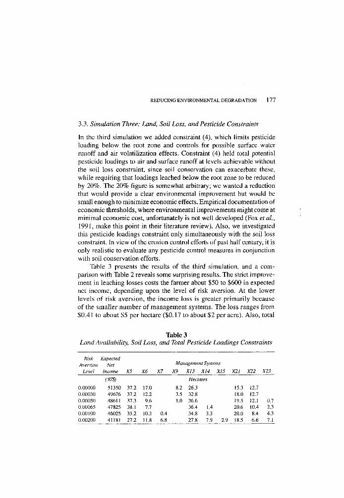
3.3. Simulation Three: Land, Soil Loss, and Pesticide Constraints

In the third simulation we added constraint (4), which limits pesticide loading below the root zone and controls for possible surface water runoff and air volatilization effects. Constraint (4) held total potential pesticide loadings to air and surface runoff at levels achievable without the soil loss constraint, since soil conservation can exacerbate these, while requiring that loadings leached below the root zone to be reduced by 20%. The 20% figure is somewhat arbitrary; we wanted a reduction that would provide a clear environmental improvement but would be small enough to minimize economic effects. Empirical documentation of economic thresholds, where environmental improvements might come at minimal economic cost, unfortunately is not well developed (Fox et ai, 1991, make this point in their literature review). Also, we investigated this pesticide loadings constraint only simultaneously with the soil loss constraint. In view of the erosion control efforts of past half century, it is only realistic to evaluate any pesticide control measures in conjunction with soil conservation efforts.

Table 3 presents the results of the third simulation, and a comparison with Table 2 reveals some surprising results. The strict improvement in leaching losses costs the farmer about $50 to $600 in expected net income, depending upon the level of risk aversion. At the lower levels of risk aversion, the income loss is greater primarily because of the smaller number of management systems. The loss ranges from $0.41 to about $5 per hectare ($0.17 to about $2 per acre). Also, total

Table 3 Land Availability, Soil Loss, and Total Pesticide Loadings Constraints


Level Income X5 X6 X7 X9 X13 X14 X15 X21 X22 X23

('87$) Hectares

0.00000 51350 37.2 17.0 8.2 26.3 15.3 12.7 0.00030 49676 37.2 12.2 3.5 32.8 18.0 12.7 0.00050 48611 37.3 9.6 1.0 36.6 19.5 12.1 0.7 0.00065 47825 38.1 7.7 36.4 1.4 20.6 10.4 2.3 0.00100 46025 35.2 10.3 0.4 34.8 3.3 20.0 8.4 4.3 0.00200 41181 27.2 11.8 6.8 27.8 7.9 2.9 18.5 6.6 7.1


erosion increased slightly but is well below the specified limit. The farmer drops management systems such as C C - R T - V T that increased leaching losses in favor of those systems (e.g., C S - C T - C N ) that prevent or reduce leaching.

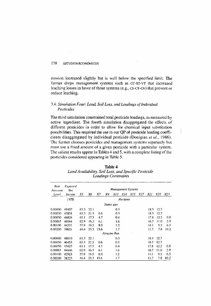
3.4. Simulation Four: Land, Soil Loss, and Loadings of Individual Pesticides

The third simulation constrained total pesticide loadings, as measured by active ingredient. The fourth simulation disaggregated the effects of different pesticides in order to allow for chemical input substitution possibilities. This required the use in our QP of pesticide loading coefficients disaggregated by individual pesticide (Donigian et aL, 1986). The farmer chooses pesticides and management systems separately but must use a fixed amount of a given pesticide with a particular system. The salient results appear in Tables 4 and 5, with a complete listing of the pesticides considered appearing in Table 5.

Table 4 Land Availability, Soil Loss, and Specific Pesticide

Loadings Constraints


Level Income X5 X6 X7 X9 X13 X14 XJ5 XJ7 X21 X22 X23

cm) Hectares

Status quo

0.00000 49407 63.3 22 A 0.3 18.3 12.7 0.00030 47851 63.3 21.5 0.6 0.3 18.3 12.7 0.00050 46824 63.1 17.5 4.7 0.4 17.8 12.2 0.8 0.00065 46064 62.9 16.3 6.1 1.6 16.7 11.0 2.9 0.00100 44321 57.9 19.5 8.0 1.2 14.1 9.5 6.5 0.00200 39621 44.4 25.3 15.6 1.7 11.7 7.8 10.2

Atrazine Ban

0.00000 48010 63.3 22.1 0.3 18.3 12.7 0.00030 46453 63.3 21.5 0.6 0.3 18.3 12.7 0.00050 45427 63.1 17.5 4.7 0.4 17.8 12.2 0.8 0.00065 44666 62.9 16.3 6.1 1.6 16.7 11.0 2.9 0.00100 42923 57.9 19.5 8.0 1.2 14.1 9.5 -6.5 0.00200 38223 44.4 25.3 15.6 1.7 11.7 7.8 10.2

REDUCING E N V I R O N M E N T A L DEGRADATION 179

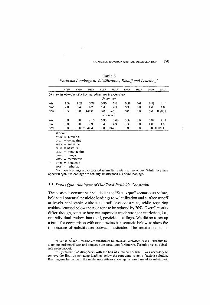
Table 5 Pesticide Loadings to Volatilization, Runoff and Leaching9

ATZN CYZN SMZN ALCR MC LR LNRN MTZN BTZN TFOS

(Air, sw in K G / H A / Y R of active ingredient; G W in M G / H A / Y R )

Status quo

Air 1.39 1.22 5.78 6.90 3.0 0.58 0.0 0.98 4.14 SW 2.0 0.4 8.7 7.4 4.3 0.3 0.0 1.0 1.8 GW 0.3 0.0 447.0 0.0 1 867.1

ATZN ban 1 0

0.0 0.0 0.0 8 800.1

Air 0.0 0.0 8.10 6.90 3.00 0.58 0.0 0.98 4.14 SW 0.0 0.0 9.9 7.4 4.3 0.3 0.0 1.0 1.8 GW 0.0 0.0 2 641.4 0.0 1 867.1 0.0 0.0 0.0 I I 800.1

Where: A T Z N = atrazine C Y Z N = cyanazine S M Z N = simazine A L C R = alachlor M C L R = metolachlor LNRN = linuron M T Z N = metribuzin BTZN = bentazon TFOS = terbufos Note: G W loadings are expressed in smaller units than sw or AIR. While they may

appear larger, G W loadings are actually smaller than AIR or sw loadings.

3.5. Status Quo: Analogue of Our Total Pesticide Constraint

The pesticide constraints included in the "Status quo" scenario, as before, held total potential pesticide loadings to volatilization and surface runoff at levels achievable without the soil loss constraint, while requiring residues leached below the root zone to be reduced by 20%. Overall results differ, though, because here we imposed a much stronger restriction, i.e., on individual, rather than total, pesticide loadings. We did so to set up a basis for comparison with our atrazine ban scenario below, to show the importance of substitution between pesticides. The restriction on in-

9 Cyanazine and simazine are substitutes for atrazine; metolachlor is a substitute for alachlor; and metribuzin and bentazon are substitutes for linuron. Terbufos has no substitute in the model.

J ( ) Cyanazine use disappears with the ban of atrazine because it was necessary to remove the limit on simazine loadings below the root zone to get a feasible solution. Banning one herbicide in the model necessitates allowing increased use of its substitutes.


dividual pesticide losses causes expected income to fall by about 4% in comparison with the Table 1 results and slows down the implementation of conservation tillage to meet the soil loss limits. Also, the management system using chemicals most intensively ( C C - R T - V T ) drops from the optimal plan.

3.6. Atrazine Ban

In the second scenario, we ban atrazine, a suspected cause of cancer; congestion of the heart, lungs, and kidneys; hypertension; muscle spasms; anorexia; and degradation of the adrenal gland ( U S E P A , 1991). Atrazine is the most widely used pesticide in U .S . com production, the most frequently detected pesticide in groundwater in most of the midwestern us. , and is ubiquitous in surface watersheds where applied ( U S E P A , 1992). The Safe Drinking Water Act requires that public utilities treat water for atrazine i f it is found in amounts greater than standards established by U S E P A . Installing advanced treatment systems to remove atrazine could result in substantial costs to utilities and their customers. Alternatives to treatment focus on controlling atrazine applications, thereby preventing or limiting its discharge into surface and ground waters. A n atrazine ban is the most extreme form of this approach.

Before looking at these results, however, the modeling of this ban warrants discussion. To get a feasible solution, it was necessary to remove the restriction on simazine loadings below the root zone. Thus, unlike the other results in this paper, those reported in the next paragraph do not hold simazine leaching below the root zone to levels achievable in the first set of simulations, before imposition of the soil loss constraint. That simply is not possible here: if we are to ban one herbicide, then we must allow increased use of substitutes. Relaxing this constraint means expressing the cost of the atrazine ban as the sum of two effects: foregone income to the farmer and net changes in pesticide loadings.

Income falls another three percent as a result of the atrazine ban. The decrease, occurs because of diminished yields and higher costs associated with the substitute herbicide, simazine (Table 5). Atrazine loadings are eliminated (as are those of cyanazine), but those of simazine to volatilization, runoff, and leaching below the root zone


increase by 40, 13, and 491 percent, respectively. The availability of a close substitute limited the economic loss to the farmer from the ban of this widely used herbicide and in fact eliminated the need to alter management systems. However, potential pesticide losses to the environment increase because of the substitution of less cost effective pesticide (e.g., simazine) for atrazine.

Health and ecosystem protection would be better served if atrazine control strategies considered both the target chemical and its substitutes. (A recent evaluation of atrazine control strategies, conducted at the regional level for the U .S . Midwest, also makes this point. See Ribaudo and Bouzaher, 1994.) Atrazine, simazine, and cynazine are all members of the triazines group and have similar leachability and toxicity properties (Gustafson, 1989; Weber, 1977). Thus, little if any environmental improvement occurs as a result of the ban. This result suggests a dilemma for regulators since banning several alternatives used for a pest problem can produce very large economic impacts (Ribaudo and Bouzaher, 1994; Osteen and Kuchler, 1986). If all triazines were to be banned, use of newer, sulfonyl herbicides (e.g., nicosulfuron and primisulfuron; not in our model) would probably increase, but at a greater cost, with a narrower window for effective application, and with a greater possibility of accelerated development of weed resistance problems. Available evidence on these newer chemicals (approved in 1990) suggests that they too have leaching potential ( U S E P A , 1992). Herbicide-resistant corn now under development might be a preferred alternative since it could promote more use of post-emergent herbicides (i.e., applied after plant emerges from soil), rather than triazines, which are pre-emergents. Post-emergent herbicides are applied in lower concentrations and later in the season; are more biodegradable; and would likely produce less leaching and runoff than triazines.

3.7. A Final Result

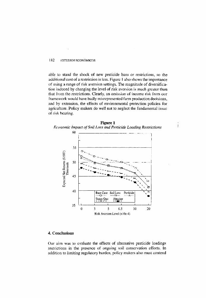
One final result puts our findings in perspective with the state of knowledge about farmers' risk attitudes. Figure 1 shows that as the level of risk aversion increases, the differences in net income under the various scenarios become smaller. This effect occurs for two reasons. First, the induced diversification causes portfolios (combinations of management systems) to become more alike. Second, diversified portfolios are better


able to stand the shock of new pesticide bans or restrictions, so the additional cost of a restriction is less. Figure 1 also shows the importance of using a range of risk aversion settings. The magnitude of diversification induced by changing the level of risk aversion is much greater than that from the restrictions. Clearly, an omission of income risk from our framework would have badly misrepresented farm production decisions, and by extension, the effects of environmental protection policies for agriculture. Policy makers do well not to neglect the fundamental issue of risk bearing.

Figure 1 Economic Impact of Soil Loss and Pesticide Loading Restrictions

60 , ,

a on

& I

55

50

45

40

35

• ® —

********

Base Case Soil Loss Pesticide s x. s

—43—, A • • • m Status Quo Atrazine

3 5 6.5 10 Risk Aversion Level (xlOe-4)

20

4. Conclusions

Our aim was to evaluate the effects of alternative pesticide loadings restrictions in the presence of ongoing soil conservation efforts. In addition to limiting regulatory burden, policy makers also must contend


with possibly opposing environmental goals. By assessing the farmer's possible response to two types of risk and to resource use restrictions, we hoped to gain a clearer picture of the cost of managing a multi-dimensional agro-environmental problem.

Some of our results were expected and suggest the fundamental soundness of our approach; others offer insights on the farmer's response to risk and resource use restrictions. With increasing levels of risk aversion, the farmer diversified production to reduce variability in net income. However, the large size of this effect, compared with any from our array of soil loss and pesticide loadings restrictions, is somewhat surprising. In particular, farmer attitudes about income risk induce enterprise diversification, while attitudes about soil loss risk appear not to matter. Imposition of a soil loss constraint, as expected, caused the farmer to shift out of conventional tillage and into systems with reduced or no-till, but our changes in the probability of meeting this constraint had no significant effect. The farmer is concerned with total soil loss over the 25-year planning horizon but not with soil loss in any given year. This finding may stem from our separate consideration of farmers' attitudes toward risk in soil loss and income, and it contrasts with the belief, expressed for example in Kramer et al. (1983), that the stochastic nature of the soil loss has a large influence on crop yields and thus on income. This is an important finding in that riskiness in soil loss has been used as a defense for subsidizing soil conservation efforts.

We also examined the effect of pesticide restrictions when soil loss constraints are already in place, as they are likely to be for some time. We found that a 20% reduction in total leaching losses cost the farmer only about $50 to $600 in expected net income ($0.41 to $5 per hectare, or $0.17 to $2 per acre), depending upon the level of risk aversion (O). At lower levels of O the farmer diversifies less and the loss in income is greater. Management systems changes are the expected response to pesticide restrictions in the absence of close substitute; systems causing smaller leaching losses replaced ones causing more, but soil erosion increased as did pesticide loadings to surface runoff.

Comparable restrictions when substitute chemicals are available are likely to cause smaller economic but larger environmental effects. A complete ban on the use of atrazine, on the other hand, caused bigger effects of both sorts. Farm income fell $1400 because of


the yield loss and higher production costs associated with the substitute herbicide, simazine. In addition, air volatilization, surface water runoff, and leaching losses from simazine increased by 40, 13, and 491 percent, respectively. A complete ban of a selected chemical may not achieve the desired goals because farmers wi l l switch to substitutes.

Limitations of this research point to directions for further work. First, because we limit only total pesticide and sediment loadings for the farm, it is possible that per hectare contamination could pose a problem at particular locations in the farm and surrounding areas. Ours is a farm level model and does not consider these important issues. Second, commodity programs that require farmers to maintain a base acreage might hinder the diversification of management systems that occurs in our model, increasing the burden of the resource use-restrictions. Uncertainty over the future forms of commodity programs would complicate efforts to include them. Also, realistic constraints on the availability of labor, machinery, or managerial skill would have the same effect. Third, we use historical variance in income as a measure of the farmer's risk rather than a field estimate that might come closer to his/her own subjective assessment. Fourth, pesticide loadings are stochastic in nature but deterministic in our model. Since the levels of pest infestations and rainfall vary and because pesticides are a risk-reducing input, pesticide loadings ideally should be incorporated in the model as stochastic rather than deterministic factors. Doing so would offset our result that pesticide applications and income risk aversion are inversely related (see Table 1). Unfortunately the data to do so—covariance matrices for pesticide loadings to environmental media for each of the pesticides—do not exist to our knowledge. In any case, the invariance of our results to changes in the soil loss risk parameter D suggests that the use of a stochastic soil loss constraint with a deterministic pesticide loadings constraint did not produce misleading results. Lastly, more research is needed to systematically measure the distribution and evolution of farmer risk preferences if research of this type is to be truly useful to policy makers. These limitations of our research stem from simplifying assumptions in an already complicated modeling effort and do not reduce the value of our findings as broad insights.

REDUCING E N V I R O N M E N T A L D E G R A D A T I O N 185

References

Anderson, G.D.; J.J. Opaluch; and W.M. Sullivan (1985). "Nonpoint Agricultural Pollution: Pesticide Contamination of Groundwater Supplies", American Journal of Agricultural Economics 67: 1238-1243.

Anderson, J.R.; J.L. Dillon; and J.B. Hardaker (1977). Agricultural Decision Analysis. Iowa State University Press.

Baumol, W.J. (1963). "An Expected Gain-Confidence Limit Criterion for Portfolio Selection", Management Science 10: 174-182.

Binswanger, H.P. (1980). "Attitudes Toward Risk: Experimental Measurement in Rural India", American Journal of Agricultural Economics 62: 395-407.

Boggess, W.G. and J.T. Ritchie (1988). "Economic and Risk Analysis of Irrigation Decisions in Humid Regions", Journal of Production Agriculture 1: 116-122.

Boussard, J. and M . Petit (1967). "Representation of Farmers' Behavior Under Uncertainty with a Focus Loss Constraint", Journal of Farm Economics 49: 869-880.

Braden, J.; G.V. Johnson; A. Bouzaher; and D. Miltz (1989). "Optimal Spatial Management of Agricultural Pollution", American Journal of Agricultural Economics 71: 404-413.

Carsel, R.F.; C.N. Smith; L .A. Mulkey; D.J. Dean; and P.P. Jowise (1986). Users' Manual for the Pesticide Root Zone Model (PRZM): Release 2. U.S.

Environmental Protection Agency Laboratory, Athens, Georgia. Chames, A. and W.W. Cooper (1959). "Chance Constrained Programming",

Management Science 6:73-79. Dillon, J.L. and P.L. Scandizzo (1978). "Risk Attitudes of Subsistence Farms in

Northeast Brazil: A Sampling Approach",7\m^nca/i Journal of Agricultural Economics 60: 425-435.

Collins, R. A. and J.C. Headley ( 1983). "Optimal Investment to Reduce the Decay Rate of Income Stream: The Case of Soil Conservation", Journal of Environmental Economics and Management 10: 60-71.

Donigian, A.S.; C.S. Raju; and R.F. Carsel (1986). Impact of Conservation Tillage on Environmental Pesticide Concentration in Three Agricultural Regions. Unpublished report. Office of Policy Analysis, U.S. EPA.

Ervin, D.E. (1982). Perceptions, Attitudes and Risk: Overlooked Variables in Formulating Public Policy on Soil Conservation and Water Quality. Staff report AGES820129, Economic Research Service, U.S. Department of Agriculture.

Fox, G.; A . Weersink; G. Sarwar; S. Duff; and W. Deen (1991). "Comparative Economics of Alternative Agricultural Production Systems: A Review", Northeastern Journal of Agricultural and Resource Economics 20: 124-142.

Freund, R.J. (1956). "The Introduction of Risk into a Programming Model", Econometrica 24: 253-263.


Gustafson, D.I. (1989). "Groundwater Ubiquity Score: A Simple Method for Assessing Pesticide Leachability", Environmental Technology and Chemistry 8: 339-357.

Hazell, P.B.R. and R.D. Norton (1986). Mathematical Programming for Economic Analysis in Agriculture, Macmillan.

Johnson, S.L.; R.M. Adams; and G.M. Perry (1991). "The On-Farm Costs of Reducing Groundwater Pollution", American Journal of Agricultural Economics 73: 1063-1073.

Kramer, R.A.; W.T. McSweeny; and R.W. Stavros (1983). "Soil Conservation with Uncertain Revenues and Input Supplies", American Journal of Agricultural Economics 65: 694-702.

Lichtenberg, E.; D. Parker; and D. Zimmerman (1988). "Marginal Analysis of Welfare Costs of Environmental Policies: The Case of Pesticide Regulation", American Journal of Agricultural Economics 70: 867-874.

Lin, W.; G.W. Dean; and C.V. Moore (1974). "An Empirical Test of Utility vs Profit Maximization in Agricultural Production", American Journal of Agricultural Economics 56: 497-508.

Markowitz, H.M. (1959). Portfolio Selection: Efficient Diversification of Investments. New York: Wiley.

Osteen, C. and F. Kuchler (1986). Potential Bans of Corn and Soybeans Pesticides: Economic Implications for Farmers and Consumers. AER-546, Economic Research Service, U.S. Department of Agriculture.

Park, W. and L. Shabman (1982). "Distributional Constraints on Acceptance of Nonpoint Pollution Controls", American Journal of Agricultural Economics 64: 455-462.

Prato, T. (1991). "Economic Feasibility of Conservation Tillage with Stochastic Yields and Erosion Rates", North Central Journal of Agricultural Economics 12: 333-344.

Ribaudo, Marc O. and Aziz Bouzaher (1944). Atrazine: Environmental Characteristics and Economics of Management. USDA/ERS Agricultural Economic Report 699.

Robison, L. and P. Brake (1979). "Application of Portfolio Theory To Farmer and Lender Behavior", American Journal of Agricultural Economics 61: 158-164.

Rubinstein, R. (1981). Simulation and the Monte Carlo Method. New York: Wiley.

Segarra, E.; R.A. Kramer; and D.B. Taylor (1985). " A Stochastic Programming Analysis of the Farm Level Implications of Soil Erosion Control", Southern Journal of Agricultural Economics 17: 147-154.

Setia, P.P. and G.V. Johnson (1988). "Soil Conservation Management Systems under Uncertainty", North Central Journal of Agricultural Economics 10: 111-124.

Shortle, J.S. and J.A. Miranowski (1987). "Intertemporal Soil Resource Use: Is It Socially Excessive?", Journal of Environmental Economics and Management 14: 99-111.


Tauer, L. (1986). "Risk Preferences of Dairy Farmers", North Central Journal of Agricultural Economics 8: 7-16.

Taylor, C.R. and K. Frohberg (1977). "The Welfare Effects of Erosion Controls, Banning Pesticides, and Limiting Pesticide Application in the Corn Belt", American Journal of Agricultural Economics 59: 25-36.

Tintner, Gerhard (1940). The Variate Difference Method. Bloomington: University of Indiana Press.

U.S. Environmental Protection Agency (1991). National Pesticide Survey: Project Summary. Office of Water (Fact Sheet).

(1994). National Water Quality Inventory: 1992 Report to Congress. Office of Water. Report Number 841-R-94-001.

(1992). Water Resources Analysis for the Triazine Herbicides. Office of Pesticide Programs.

Venkataraman, R.R. (1988 ). Impact of Tenure and Uncertainty on the Choice of Optimal Soil Erosion Control Measures. Ph.D. Dissertation (unpublished), Department of Agricultural Economics, University of Illinois.

Von Neumann, J. and O. Morgenstern (1944). Theory of Games and Economic Behavior, Princeton University Press.

Weber, J.B. "The Pesticide Scorecard", Environmental Science and Technology 11: 756-761.

Wischmeier, W.H. and D.D. Smith (1978). Predicting Rainfall Erosion Losses— A Guide to Conservation Planning. Agricultural Handbook 537, Science and Educational Administration, USDA.

Yeh, G.T. (1986). Analytical Transient One-, Two-, Three-Dimensional Simulation of Waste Treatment in the Aquifer System. ORNL-5602. Oak Ridge National Laboratory, Oak Ridge, TN.

on-farm cost os f reducing environmental...

Documents