on hierarchical diameter-clustering and the supplier problem

Theory Comput Syst (2009) 45: 497–511DOI 10.1007/s00224-009-9186-6

On Hierarchical Diameter-Clusteringand the Supplier Problem

Aparna Das · Claire Kenyon-Mathieu

Published online: 27 January 2009© Springer Science+Business Media, LLC 2009

Abstract Given a data set in a metric space, we study the problem of hierarchicalclustering to minimize the maximum cluster diameter, and the hierarchical k-supplierproblem with customers arriving online.

We prove that two previously known algorithms for hierarchical clustering, one(offline) due to Dasgupta and Long and the other (online) due to Charikar, Chekuri,Feder and Motwani, output essentially the same result when points are considered inthe same order. We show that the analyses of both algorithms are tight and exhibita new lower bound for hierarchical clustering. Finally we present the first constantfactor approximation algorithm for the online hierarchical k-supplier problem.

Keywords Hierarchical clustering · Approximation algorithm · Online algorithm

1 Introduction

Clustering is the partitioning of data points into disjoint clusters (or groups) accord-ing to similarity [1, 9]. For example if the data points are books, a 2-clustering mightconsist of the clusters fiction, and non-fiction. In this way clustering can provide aconcise view of large amounts of data. In many application domains it is useful tobuild a partitioning of the data that starts with broad categories which are graduallyrefined thus allowing the data to be viewed simultaneously at different levels of con-ciseness. This calls for a hierarchical or nested clustering of the data where clustershave subclusters, these have subsubclusters, and so on. For example a hierarchicalclustering might first separate the books into clusters fiction and non-fiction, then

A. Das (�) · C. Kenyon-MathieuBrown University, Providence, RI 02918, USAe-mail: [email protected]

C. Kenyon-Mathieue-mail: [email protected]

mailto:[email protected]

mailto:[email protected]

498 Theory Comput Syst (2009) 45: 497–511

separate the fiction cluster into classics and non-classics and the non-fiction clusterinto math, science and history, and so on. More formally, a hierarchical clusteringof n data points is a recursive partitioning of the points into 1,2,3,4, . . . , n clusterssuch that the (k + 1)th clustering is obtained by dividing one of the clusters of thekth clustering into two parts, thus making the clustering gradually more fine-grained[5, Sect. 10.9]. This framework has long been popular among statisticians, biologists(particularly taxonomists) and social scientists [10].

A criterion commonly used to measure the quality of a clustering is the maxi-mum cluster diameter, where the diameter of a cluster is the distance between thetwo farthest points in the cluster. The goal is to find clusterings which minimize themaximum cluster diameter, thus similar points are placed in the same cluster whiledissimilar points are separated. In this paper, we focus on the hierarchical diameter-clustering problem: finding a hierarchical clustering where the value of the clusteringis the maximum cluster diameter.

Every associated k-clustering of the hierarchical clustering should be close tothe optimal k-clustering, where the optimal k-clustering is the one that minimizesthe maximum cluster diameter. The competitive ratio of a hierarchical clusteringalgorithm A is the supremum, over n and over input sets S of size n, of thequantity maxk∈[1,n] Ak(S)/OPTk(S), where OPTk(S) is the value of the optimalk-clustering of S and Ak(S) is the value1 of the k-clustering constructed by algo-rithm A. Thus a hierarchical clustering algorithm with a small competitive ratio, pro-duces k-clusterings which are close to the optimal for all 1 ≤ k ≤ n.

The hierarchical diameter-clustering problem was studied in work by Dasguptaand Long [4] and by Charikar, Chekuri, Feder and Motwani [2]. A simple and com-monly used algorithm for this problem is the greedy “agglomerative” algorithm [5],which starts with n singletons clusters and repeatedly merges the two clusters whoseunion has smallest diameter. However, it is proved in [4] that this algorithm has com-petitive ratio �(logk). The authors then propose a better, constant-factor algorithm,inspired by the “divisive” k-clustering algorithm of Gonzalez [6]. The algorithm pro-posed in [2] is instead “coalescent” and may be partially inspired by a k-clusteringalgorithm by Hochbaum and Shmoys [8]. Superficially, the hierarchical k-clusteringalgorithms presented in the two papers look quite different. Quoting [4]: “the earlierwork of [2] uses similar techniques for a loosely related problem, and achieves thesame bounds”. Indeed, both papers present a 8 competitive deterministic algorithmand a 2e competitive randomized variant. Additionally, the algorithm from [2] fo-cuses on online clustering, where points arrive one by one in an arbitrary sequence.We refer to the algorithm from [2] as the tree-doubling algorithm and to the algorithmfrom [4] as the farthest algorithm. Here are the main results from [2, 4].

Theorem 1 For the hierarchical diameter-clustering problem, the farthest algo-rithm is 8-competitive, in its deterministic form and 2e-competitive in its randomizedform [4].

The tree doubling algorithm is 8-competitive, in its deterministic form and 2e-competitive in its randomized form [2].

1If A is randomized, then Ak(S) should be replaced by E(Ak(S)).

Theory Comput Syst (2009) 45: 497–511 499

Our first contribution is to formally relate the two algorithms. Their specificationcontains some non-deterministic choices: the farthest algorithm starts from an arbi-trary point, and the tree-doubling algorithm considers the points in arbitrary order.Assuming some conditions which remove the non-determinism, we prove that bothin the deterministic and in the randomized cases the clustering produced by the far-thest algorithm is always a refinement of the clustering produced by the tree-doublingalgorithm, where refinement is defined as follows:

Definition 1 A partition F1,F2, . . . Fl is a refinement of a partition D1,D2, . . .Dk

iff ∀i ≤ l, ∃j ≤ k such that Fi ⊆ Dj .

The farthest clustering is a refinement and not equivalent to the tree doubling clus-tering because the farthest algorithm always outputs a k-clustering with exactly k

clusters, where as the tree doubling algorithm outputs one with at most k clusters.

Theorem 2 (Refinement) Assume that the first two points labeled by the farthestalgorithm have distance equal to the diameter of the input. Also assume that thetree-doubling algorithm considers points in the order in which they were labeledby the farthest algorithm. Moreover, in the randomized setting, assume that the twoalgorithms choose the same random value r .2

Then, for every k, the k-clustering produced by the farthest (deterministic or ran-domized) algorithm is a refinement of the k-clustering produced by the tree-doubling(deterministic or randomized) algorithm.

With this interpretation, we see that the competitive ratio of the farthest algorithmcan be seen as a corollary of the competitive ratio of the tree-doubling algorithm.Could it be that the farthest algorithm is actually better? We answer this question inthe negative by proving that the analysis of the farthest algorithm in [4] is tight.

Theorem 3 (Tightness) The competitive ratio3 of the deterministic farthest algorithmis at least 8.

This means that the 8 competitive ratio upper bound for the farthest algorithm istight, and, by the refinement theorem, the 8 competitive ratio upper bound for thetree-doubling algorithm is also tight. Proving tightness of the randomized variantsare open.

Can the competitive ratio be improved? We turn to the question of what is the bestcompetitive ratio achievable for any hierarchical clustering algorithm with no compu-tational restrictions. In other words, what is the best we can expect from a hierarchicalclustering algorithm if it is allowed to have non-polynomial running time? We provethat no deterministic algorithm can achieve a competitive ratio better than 2, and norandomized algorithm can achieve competitive ratio better than 3/2. (Note that the

2The significance of parameter r will be explained in Sect. 2.3Charikar et al. [2] present a lower bound of 8 for their clustering algorithm, however it applies to theonline setting but not to the hierarchical setting and does not extend to the tree-doubling algorithm.


lower bounds proved in [2] apply to the online model only and thus are incomparableto our lower bounds.)

Theorem 4 (Hierarchical lower bound) No deterministic (respectively randomized)hierarchical clustering algorithm can have competitive ratio better than 2 (respec-tively better than 3/2), even with unbounded computational power.

How general are these techniques? In our final contribution, we extend the tree-doubling algorithm to design the first constant factor approximation algorithm for theonline hierarchical supplier problem.

In the standard (offline, non hierarchical) k-supplier problem, we are given a set S

of suppliers and a set C of customers and the distances between all customer-supplierpairs. We wish to select a set Sk of k suppliers and an assignment of each customer c

to a supplier f (c) in Sk so as to minimize the maximum distance from any customerto its supplier, maxc∈C d(c, f (c)). For example the task of segmenting customers intoa small number, k, market segments can be modeled as a k-supplier problem wherethe suppliers are a set of fixed templates representing different markets and the goal isto match markets to customers based on their buying patterns (the distance measure).A 3-approximation algorithm for the k-supplier problem is mentioned in [7].

In the more difficult online hierarchical setting, the set S of suppliers is known inadvance but new customers arrive as time goes on, so C is a sequence of customers.When a new customer arrives, it is either assigned to one of the existing open sup-pliers, or a new supplier is opened to serve this customer. If opening a new supplierresults in more than k open suppliers then two existing open suppliers merge theircustomer lists, and one of them closes. This requirement ensures that the hierarchicalcondition is satisfied, i.e. that Si−1 ⊆ Si and that for each supplier s ∈ Si \ Si−1, allthe customers assigned to s are assigned to the same supplier in Si−1. For example,suppose customers arrive over time to use resources and we would like to dynami-cally increase/decrease the total number of resources allocated without having to doextensive recomputation. Using the hierarchical supplier solution, this only requiressplitting/merging the customers currently assigned to one of the resources. The onlinehierarchical model is an increasingly important framework for clustering problems,where there is a requirement to gather and categorize large amounts of data on the fly(see [12] for example).

Using the tree-doubling algorithm as a subroutine, we obtain a constant-factor ap-proximation algorithm for the online hierarchical supplier problem. (Note that in theoffline case, we could equivalently have used the farthest algorithm as a subroutine.In fact, we conjecture that in the offline case, a similar result may also be obtainableusing methods from [3, 11].)

Theorem 5 (Online hierarchical supplier) For the online hierarchical k-supplierproblem, there exists a deterministic 17-approximation algorithm and a randomized(1 + 4e) = 11.87-approximation algorithm.


2 Review of the Hierarchical Clustering Algorithms

2.1 The Farthest Algorithm from [4]

The input is a set of n points {x1, . . . xn} with associated distance metric d . The algo-rithm has three main steps:

Labeling the Points Take an arbitrary point and label it 1. Give label i for i ∈{2, . . . , n}, to the point which is farthest away from the previously labeled points.Let di denote the distance from i to the previous i − 1 labeled points, i.e di =min1≤j≤i−1 d(i, j). Thus d2 = d(1,2).

Assigning Levels to Labelled Points For labelled point 1, set level(1) = 0. For la-belled point i ∈ {2, . . . , n}, set level(i) = �log2(d2/di)� + 1.

Organizing Labelled Points into a Tree Organize the points into a tree referred toas the �′-tree. Place point 1 as the root of the �′-tree. For each point i ∈ {2, . . . , n},define its parent, π ′(i), to be the point closest to i among the points with level strictlyless than level(i). Later, in order to compare the farthest algorithm with the tree dou-bling algorithm we set a specific tie breaking scheme for choosing the parent for anode. Insert points i > 1 into the �′-tree in order of increasing levels connecting eachpoint i with an edge to its parent π ′(i).

The hierarchical clustering is represented implicitly in the �′-tree. To obtain thek-clustering (of the hierarchical clustering) remove edges (i,π ′(i)), for i ∈ {2, . . . , k}from the �′-tree. Deleting these k − 1 edges splits the �′-tree into k connected com-ponents such that points {1, . . . , k} are in separate components. The components arereturned as the k clusters.

It is easy to verify that this defines a hierarchical clustering, and [4] proves that itsatisfies the following properties. The distances (di)i are a monotone non-increasingsequence, and the levels (level(i))i are a monotone non-decreasing sequence. Thedefinition of levels imply the following bounds on di .

d2/2level(i) < di ≤ d2/2level(i)−1. (1)

In addition [4] proves that:

d(i,π ′(i)) ≤ d2/2level(i)−1. (2)

Dasgupta and Long [4] also present a randomized variant of the farthest algorithm,where the only difference is in the definition of levels. A value r is chosen uniformlyat random from the interval [0,1], and the levels are now defined by: level(1) = 0 andlevel(i) = �ln(d2/di) + r� + 1. The monotonicity properties are unchanged; and thetwo inequalities are replaced by the following.

erd2/elevel(i) < di ≤ erd2/e

level(i)−1 and d(i,π ′(i)) ≤ erd2/elevel(i)−1. (3)


2.2 The Tree-Doubling Algorithm from [2]

Here the input consists of a sequence of n points {x1, . . . , xn} with associated distancemetric d . Let � denote the diameter of the points. The algorithm considers the pointsone by one in an online fashion and maintains a certain infinite rooted tree which werefer to as the T + tree. Each node in T + is associated to a point, and the set of nodesassociated to the same point forms an infinite path in the tree. The first point is placedat depth 0 as the root of T +, and a copy of this point is placed at each depth d > 0along with a parent edge to the copy at depth d − 1. When a new point p arrives itis inserted at a depth dp , as defined by the insertion rule given below. A copy of p isplaced at each depth d > dp with a parent edge to the copy of p at depth d − 1.

(Insertion rule) Find the largest depth d with a point q such that dist(p, q) ≤�/2d . Point p is inserted into depth dp = d + 1 with a parent edge to q .

To obtain a k-clustering, find the maximum depth d in T + which has at most k

nodes. Delete all tree nodes at depth less than d . This leaves ≤ k subtrees rooted atthe points at depth d . Delete all multiple copies of points from the subtrees and returnthese as the clusters.

By [2], the following properties are maintained as nodes are added to T +:

Property 1 (Close-parent property) Points at depth d are at distance at most �/2d−1

from their parents.

Property 2 (Far-cousins property) Points at depth d are at distance greater than �/2d

from one another.

Charikar et al. [2] also presents a randomized variant, where the only difference isin the insertion rule. A value r is chosen uniformly at random from the interval [0,1],and the insertion rule is now: Find the largest depth d that contains a point q suchthat dist(p, q) ≤ er�/ed . Point p is inserted into depth dp = d + 1 with a parentedge to q .

The properties are replaced by the following.

Property 3 Points at depth d are at distance at most er�/ed−1 from their parents,and at distance greater than er�/ed from one another.

3 Proof of the Refinement Theorem

3.1 Proof of the Deterministic Version

To relate the farthest and tree doubling algorithms we first make some assumptionsabout their nondeterministic choices. The farthest algorithm starts its labelling at anarbitrary point. We will assume the first point labelled by the farthest algorithm is atdistance � from the second point labelled by the algorithm and thus d2 = �. Thetree doubling algorithm receives its input points in an arbitrary order. We assumethat points arrive to the tree-doubling algorithm in the order they are labeled by the


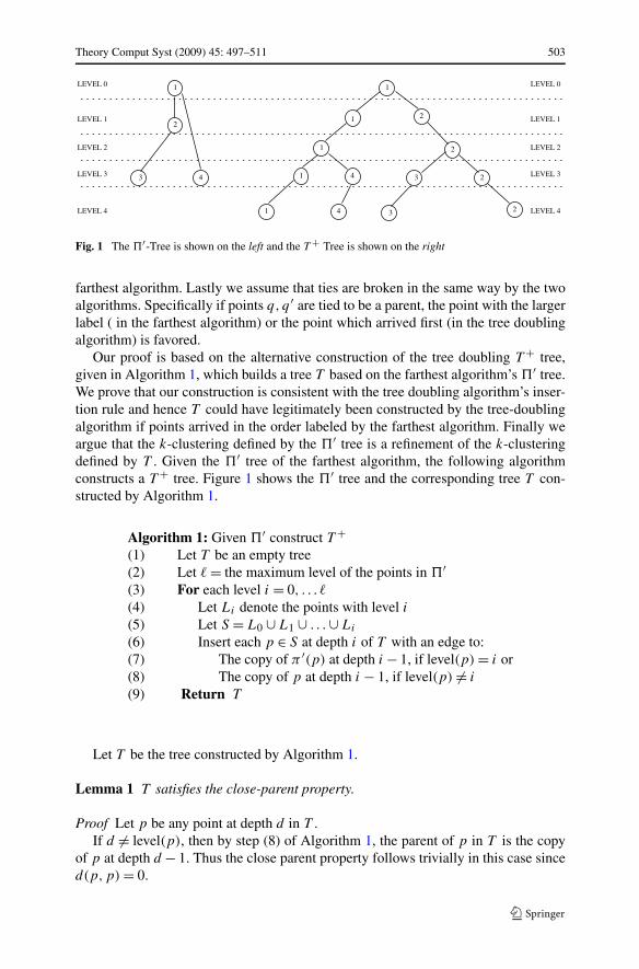
Fig. 1 The �′-Tree is shown on the left and the T + Tree is shown on the right

farthest algorithm. Lastly we assume that ties are broken in the same way by the twoalgorithms. Specifically if points q, q ′ are tied to be a parent, the point with the largerlabel ( in the farthest algorithm) or the point which arrived first (in the tree doublingalgorithm) is favored.

Our proof is based on the alternative construction of the tree doubling T + tree,given in Algorithm 1, which builds a tree T based on the farthest algorithm’s �′ tree.We prove that our construction is consistent with the tree doubling algorithm’s inser-tion rule and hence T could have legitimately been constructed by the tree-doublingalgorithm if points arrived in the order labeled by the farthest algorithm. Finally weargue that the k-clustering defined by the �′ tree is a refinement of the k-clusteringdefined by T . Given the �′ tree of the farthest algorithm, the following algorithmconstructs a T + tree. Figure 1 shows the �′ tree and the corresponding tree T con-structed by Algorithm 1.

Algorithm 1: Given �′ construct T +(1) Let T be an empty tree(2) Let � = the maximum level of the points in �′(3) For each level i = 0, . . . �

(4) Let Li denote the points with level i

(5) Let S = L0 ∪ L1 ∪ . . . ∪ Li

(6) Insert each p ∈ S at depth i of T with an edge to:(7) The copy of π ′(p) at depth i − 1, if level(p) = i or(8) The copy of p at depth i − 1, if level(p) �= i

(9) Return T

Let T be the tree constructed by Algorithm 1.

Lemma 1 T satisfies the close-parent property.

Proof Let p be any point at depth d in T .If d �= level(p), then by step (8) of Algorithm 1, the parent of p in T is the copy

of p at depth d − 1. Thus the close parent property follows trivially in this case sinced(p,p) = 0.


Otherwise, d = level(p). By step (7) of Algorithm 1 parent(p) = π ′(p). Applying(2) with d2 = �, we have that, d(p,π ′(p)) ≤ �/2level(p)−1. Substituting level(p) =d and π ′(p) = parent(p), we get: d(p,parent(p)) ≤ �/2d−1. �

Lemma 2 T satisfies the insertion rule.

Proof By steps (3–6) of Algorithm 1 if level(p) = d , then p appears in T for the firsttime at depth d and its parent q is π ′(p).

Since level(π ′(p)) < level(p), a copy of π ′(p) must be at depth d − 1 in T . SinceT satisfies the close-parent property, d(p,π ′(p)) ≤ �/2d−1. Thus π ′(p) is qualified(distance-wise) to be the parent of p according to the insertion rule.

To show that insertion rule is satisfied we need to show that when p first arrives,there was no other point at a depth higher than d − 1 which was close enough to p tobe its parent. Let q ′ be any point at depth j > d −1, which arrived before p. Note thatq ′ ∈ {1, . . . , p − 1} since by assumption points arrive in the order they are labelled bythe farthest algorithm. We need to show that d(p,q ′) > �/2j . Note that by definitionof dp , d(p,q ′) ≥ minj∈[1,p−1] d(p, j) = dp . Using the fact that level(p) = d and (1)with d2 = � we get

dp > �/2level(p) = �/2d .

Combining the two statements above we have that

d(p,q ′) ≥ dp > �/2d ≥ �/2j ,

where the last inequality follows since j > d − 1 ⇒ j ≥ d . Since d(p,q ′) > �/2j

point q ′ cannot be parent of p. �

We have shown that T satisfies the insertion rule and thus it can be constructed bythe tree-doubling algorithm when the assumptions of Theorem 2 hold. Thus for therest of the proof assume that the tree doubling algorithm constructs T .

Given k, the farthest algorithm removes exactly k − 1 edges from the �′ treeand returns a clustering F(k) with exactly k clusters. The tree-doubling algorithmlooks for the deepest level of the T tree with at most k nodes and thus returns aclustering D(k) with ≤ k clusters. We first show the two clusterings D(k) and F(k)

are equivalent when they both have exactly k clusters. The refinement property thenfollows easily.

Lemma 3 Let k be such that the tree doubling tree T has a depth d with exactly k

vertices, then the clusterings F(k) and D(k) are the same.

Proof Let F1, . . . Fk be the clusters returned by the farthest algorithm, where Fi con-tains point i. Let D1, . . .Dk be the clusters returned by the tree-doubling algorithm,where the cluster are defined by the k points at depth d in T . Since depth d containsexactly k vertices, the monotonicity of (level(i))i implies that these points must beexactly the points 1, . . . , k. We will show that for any 1 ≤ i ≤ k if a point, x, is inDi then x ∈ Fi . Since the k-clustering is a partition of the points, this immediatelyimplies that Di = Fi for all 1 ≤ i ≤ k.


Let x be a point in Di . Since Di contains the points in the subtree under i, thereis a i-to-x path P = (i = p1,p2, . . . pl = x) in T . Let S = (i = s1, s2, . . . sm = x)

be the sequence of points obtained by deleting all repetitions of points from P . Bythe construction of T we have that sj = π ′(sj+1) for all 1 ≤ j ≤ m which impliesthat S is a valid i-to-x path in the �′-tree. Since depth d of T contains all points in{1, . . . , k}, only point i can appear in sequence S. Thus none of the points {1, . . . , k}except i are in the i-to-x path in �′ tree. This implies that x ∈ Fi . �

Corollary 1 Let k1 be an input such that D(k1) has strictly less than k1 clusters. Letk2 be the minimum input such that k2 > k1 and D(k2) has exactly k2 clusters. ThenD(k1) � F(k1) � D(k2), where A � B stands for “B is a refinement of A”.

Proof Let k < k1 be the number of clusters in D(k1). Thus D(k1) = D(k) and T

has a level with exactly k vertices. By Lemma 3, F(k) = D(k). By definition ofa hierarchical clustering, F(k) � F(k1) as k < k1. Thus we have D(k1) = D(k) =F(k) � F(k1).

Similarly, on input k2, the tree-doubling algorithm produces a clustering withexactly k2 clusters which implies that T has a level with exactly k2 vertices. ByLemma 3, F(k2) = D(k2). By definition of a hierarchical clustering, F(k1) � F(k2)

as k1 < k2. Thus we have F(k1) � F(k2) = D(k2). �

3.2 Proof of the Refinement Theorem, Randomized Version

Suppose the random parameter r in the randomized versions of the farthest and thetree-doubling algorithms is chosen to have the same value. Then Lemma 3 and Corol-lary 1 also apply to the randomized algorithms. The only change to the analysis is touse inequalities (3) instead of inequalities (2) and (1) in the proof of correctness forAlgorithm 1.

3.3 Nondeterministic Choices

To prove the refinement theorem, we made some assumptions about the nondeter-ministic choices of the two algorithms. But how much do these choices affect theperformance of the algorithms?

The first point chosen by the farthest algorithm determines the value of d2 andthis in turn determines the level threshold of the �′ tree, i.e. level one contains thepoints which are at distance [d2, d2/2) from previously labelled points and level twocontains points which are at distance [d2/2, d2/22) from previously labelled pointsand so on. The initial point can affect the performance of the farthest algorithm by afactor up to 8 as demonstrated on the example we present in Sect. 4, Fig. 2. On thisexample when the farthest algorithm chooses initial point p1 it outputs a 5-clusteringwhich has cost arbitrarily close to 8 OPT. However the optimal 5-clustering can beobtained if p4 is chosen as the initial point.

Points arrive to the tree doubling algorithm in an arbitrary order. How much canthe ordering of points affect the performance of the tree doubling algorithm? By therefinement theorem, if points arrive in the order labelled by the farthest algorithm,


there is always a way to break ties so that the tree doubling clustering is no betterthan the farthest clustering. However the arrival order of points can help the treedoubling algorithm perform better than the farthest algorithm. We demonstrate thison the tight example presented in Sect. 4, Fig. 2. If the points arrive as labelled by thefarthest algorithm, the tree doubling and the farthest 5-clustering have cost 8 OPT,while if the order starts with p2,p5,p

′5, then tree doubling can construct the cost

2 OPT, 5-clustering:{(p2

),(p3

),(p′

3

)(p1,p4,p5, q1 . . . qn

),(p′

1,p′4,p

′5, q

′1 . . . q ′

n

)}.

Combining these observations, we see that the farthest algorithm can produce clus-terings which are 8 times better than the tree doubling algorithm clusterings if the far-thest algorithm starts with the best possible initial point and the tree doubling is givenits points in the worst possible ordering. On the other hand the tree doubling cluster-ings can be 4 times better than the farthest clusterings when its points are orderedfavorably and the farthest algorithm starts at the worst possible initial point.

4 Proof of the Tightness Theorem

We will prove that, for any ε > 0, there exists an input on which the farthest algo-rithm produces a hierarchical clustering where the k = 5 clustering is worse than theoptimal 5-clustering by a factor of at least 8 − 4ε.

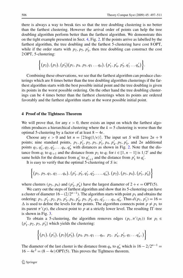
Choose any ε > 0 and let n = �2 log(1/ε)�. The input set S will have 2n + 9points; nine standard points, p1,p

′1,p2,p3,p

′3,p4,p

′4,p5,p

′5, and 2n additional

points q1, q′1, q2, q

′2, . . . qn, q

′n with distances as shown in Fig. 2. Note that the dis-

tance from qi to qi+1 and the distance from p1 to qi for i ∈ [1, n − 1] is 1/2i and thesame holds for the distance from q ′

i to q ′i+1 and the distance from p′

1 to q ′i .

It is easy to verify that the optimal 5-clustering of S is:{(p1,p5, q1, q2 . . . qn

),(p′

1,p′5, q

′1, q

′2, . . . , q

′n

),(p2

),(p3,p4

),(p′

3,p′4

)}

where clusters (p3,p4) and (p′3,p

′4) have the largest diameter of 2 + ε = OPT(5).

We carry out the steps of farthest algorithm and show that its 5-clustering can havea cluster of diameter 16−(2/2n−1). The algorithm starts with point p1 and obtains theordering: p1,p

′1,p2,p3,p

′3,p4,p

′4,p5,p

′5, q1, q

′1, . . . qn, q

′n. Thus d(p1,p

′1) = 16 =

� is used to define the levels for the points. The algorithm connects point p �= p1 toits parent π ′(p), the closest point to p at a strictly lower level. The resulting �′-treeis shown in Fig. 3.

To obtain a 5-clustering, the algorithm removes edges (pi,π′(pi)) for pi ∈

{p′1,p2,p3,p

′3} which yields the clustering:

{(p1

),(p′

1

),(p3

)(p′

3

),(p4,p5, q1 . . . qn, p2, p′

4,p′5, q1 . . . q ′

n,)}

The diameter of the last cluster is the distance from qn to q ′n which is 16 − 2/2n−1 =

16 − 4ε2 = (8 − 4ε)OPT(5). This proves the Tightness theorem.


Fig. 2 Graph for tight example

Fig. 3 �-Tree for tight example

5 Proof of the Hierarchical Lower Bound Theorem

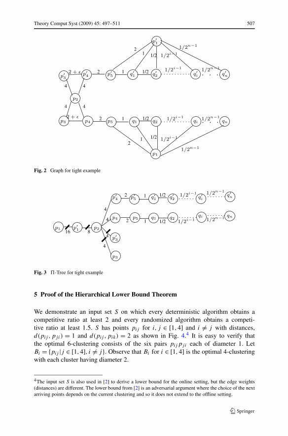
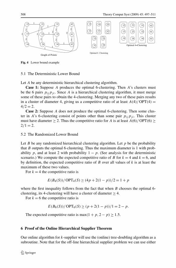
We demonstrate an input set S on which every deterministic algorithm obtains acompetitive ratio at least 2 and every randomized algorithm obtains a competi-tive ratio at least 1.5. S has points pij for i, j ∈ [1,4] and i �= j with distances,d(pij ,pji) = 1 and d(pij ,pik) = 2 as shown in Fig. 4.4 It is easy to verify thatthe optimal 6-clustering consists of the six pairs pijpji each of diameter 1. LetBi = {pij |j ∈ [1,4], i �= j}. Observe that Bi for i ∈ [1,4] is the optimal 4-clusteringwith each cluster having diameter 2.

4The input set S is also used in [2] to derive a lower bound for the online setting, but the edge weights(distances) are different. The lower bound from [2] is an adversarial argument where the choice of the nextarriving points depends on the current clustering and so it does not extend to the offline setting.


Fig. 4 Lower bound example

5.1 The Deterministic Lower Bound

Let A be any deterministic hierarchical clustering algorithm.Case 1: Suppose A produces the optimal 6-clustering. Then A’s clusters must

be the 6 pairs pijpji . Since A is a hierarchical clustering algorithm, it must mergesome of these pairs to obtain the 4-clustering. Merging any two of these pairs resultsin a cluster of diameter 4, giving us a competitive ratio of at least A(4)/OPT(4) =4/2 = 2.

Case 2: Suppose A does not produce the optimal 6-clustering. Then some clus-ter in A’s 6-clustering consist of points other than some pair pijpji . This clustermust have diameter ≥ 2. Thus the competitive ratio for A is at least A(6)/OPT(6) ≥2/1 = 2.

5.2 The Randomized Lower Bound

Let B be any randomized hierarchical clustering algorithm. Let p be the probabilitythat B outputs the optimal 6-clustering. Thus the maximum diameter is 1 with prob-ability p, and at least 2 with probability 1 − p. (See analysis for the deterministicscenario.) We compute the expected competitive ratio of B for k = 4 and k = 6, andby definition, the expected competitive ratio of B over all values of k is at least themaximum of these two values.

For k = 4 the competitive ratio is

E(B4(S))/OPT4(S) ≥ (4p + 2(1 − p))/2 = 1 + p

where the first inequality follows from the fact that when B chooses the optimal 6-clustering, its 4-clustering will have a cluster of diameter ≥ 4.

For k = 6 the competitive ratio is

E(B6(S))/OPT6(S) ≥ (p + 2(1 − p))/1 = 2 − p.

The expected competitive ratio is max(1 + p,2 − p) ≥ 1.5.

6 Proof of the Online Hierarchical Supplier Theorem

Our online algorithm for k-supplier will use the (online) tree-doubling algorithm as asubroutine. Note that for the off-line hierarchical supplier problem we can use either


the tree-doubling or the farthest algorithm and achieve the same performance guar-antees described below. In fact, we conjecture that in the offline case, a similar resultmay also be obtainable using methods from [3, 11].

6.1 The Algorithm

We denote a supplier as active if it is the closest supplier to one of the currentcustomers. Throughout the algorithm, we will maintain a hierarchical clustering ofthe active suppliers by inserting them into the (deterministic or randomized) tree-doubling algorithm tree T +.

When a new customer c arrives, we find the supplier s who is closest to c. If s is notyet in T +, we mark s as an active supplier and add s to T + (using the deterministicor randomized tree-doubling algorithm).

To obtain a hierarchical k-supplier solution, find the largest depth d in T + whichcontains k′ ≤ k active suppliers s1, s2, . . . sk′ and output these suppliers. For eachcustomer c with closest supplier s0, assign c to si for i ∈ [1, k′], if s0 = si or if s0 isin the subtree below si in depth d of T +.

6.2 The Deterministic Analysis

Suppose d is the largest depth containing at most k active suppliers. Let s (at depthd) be the supplier that customer c was assigned to and s0 be the active supplier thatc is closest to. Then there is a s0-to-s path in T +. Let s0, s1, . . . sp be the sequenceof the suppliers on the s0-to-s path, where sp = s. By the triangular inequality, thedistance from c to s can be bounded as:

d(c, s) ≤ d(c, s0) +p−1∑i=0

d(si, si+1). (4)

Let � be the maximum distance between any two suppliers. By the close-parentproperty of the tree-doubling algorithm, the distance from si to si+1 for i ∈ [0,p − 1]is at most �/2depth(si )−1. Since the depths of suppliers on the s0-to-s path are strictlydecreasing, and sp−1 is on level d + 1, we have that,

p−1∑i=0

d(si, si+1) ≤ �

2depth(sp−1)−1(1 + 1/2 + 1/4 + . . .) ≤ 2

�

2d. (5)

Now we derive two lower bounds for OPTk . First, since s0 is the closestsupplier to c, we have that OPTk ≥ d(c, s0). Next, since d is the largest depthin T + with at most k active suppliers, depth d + 1 contains at least k + 1 ac-tive suppliers, s1, s2, . . . , sk+1. Using Lemma 4, we have OPTk ≥ δ/4 where δ =min1≤i<j≤k+1 d(si, sj ). By the Far-Cousins property of T +, δ is at least �/2d+1.Applying these bounds we obtain

d(c, s) ≤ d(c, s0) + 2�

2d≤ OPTk + 4δ.


Lemma 4 below shows that δ ≤ 4 OPTk . Thus the final result that d(c, s) ≤17 OPTk follows as a corollary to Lemma 4.

Lemma 4 Let d be the largest depth in T + with at most k active suppliers and lets1, s2, . . . , sk+1 be active suppliers at depth d + 1. Let δ = min1≤i<j≤k+1 d(si, sj ),and OPTk be the maximum distance from a customer to a supplier in the optimalk-supplier solution. Then δ ≤ 4 OPTk .

Proof Since suppliers s1, s2, . . . , sk+1 are active, each of them is the closest supplierto some customer ci . The solution OPTk uses at most k suppliers, so it will have toassign two of those customers, ci and cj , to the same supplier s∗. Thus,

OPTk ≥ max(d(ci, s∗), d(cj , s

∗)) ≥ (d(ci, s∗) + d(cj , s

∗))/2.

Applying the triangle inequality on d(si, sj ) we have that:

d(si, sj ) ≤ d(si, ci) + d(ci, s∗) + d(s∗, cj ) + d(cj , sj )

Using the fact that si is the closest supplier to ci and sj is closest for cj , we obtain

δ ≤ d(si, sj ) ≤ 2(d(ci, s∗) + d(cj , s

∗)) ≤ 4 OPTk . �

6.3 The Randomized Analysis

Equation (4) still holds. Instead of (5) we now have:

p−1∑i=0

d(si, si+1) ≤ er�

edepth(sp−1)−1(1 + 1/e + 1/e2 + . . .) ≤ e

e − 1

er�

ed.

Now, by Property 3 the minimum distance δ between s1, . . . , sk+1 satisfies er�/

ed+1 < δ ≤ er�/ed . Write δ = eεer�/ed+1, where ε is distributed uniformlyin [0,1). In expectation we have

E(er�/ed+1) = δ

∫ 1

0e−εdε = δ

e − 1

e.

Lemma 4 still holds, so we finally get:

E(d(c, s)) ≤ d(c, s0) + e

e − 1E

(er�

ed

)≤ OPTk + e

e − 1eδ

e − 1

e≤ (1 + 4e)OPTk .

7 Conclusions and Open Questions

Hierarchical clustering provides a useful way to view large amounts of data in anorganized manner and is popular among statisticians, biologists and social scien-tists [10]. In this work we have studied this problem when the objective is to minimize


the maximum cluster diameter and showed that two previously known algorithms,tree doubling [2] and farthest algorithm [4] produce essentially the same output. Bothalgorithms also work for the closely related objective of minimizing the maximumcluster radius, where the radius of a cluster is defined as the maximum distance froma designated center point to other points in the cluster. Our result that the farthestclustering is a refinement of the tree doubling clustering extend to radius objective.We also showed that the analyses of both algorithms are tight under the diameter ob-jective. However the example we used to show tightness does not extend to the radiusobjective and finding a tight example for this remains an open question.

We exhibited new lower bounds for hierarchical clustering for the diameter ob-jective. Do similar lower bounds exist for the radius objective? The derivation of ourbounds assumed no computational restrictions on the algorithm, however it might bepossible to get stronger lower bounds by placing such restrictions.

References

1. Arabie, P., Hubert, L.J., De Soete, G. (eds.): Clustering and Classification. World Scientific, RiverEdge (1998)

2. Charikar, M., Chekuri, C., Feder, T., Motwani, R.: Incremental clustering and dynamic informationretrieval. SIAM J. Comput. 33(6), 1417–1440 (2004)

3. Chrobak, M., Kenyon, C., Noga, J., Young, N.E.: Online medians via online bribery. Lect. Not. Com-put. Sci. 3887, 311–322 (2006). Latin American Theoretical Informatics (2006)

4. Dasgupta, S., Long, P.: Performance guarantees for hierarchical clustering. J. Comput. Syst. Sci.70(4), 555–569 (2005)

5. Duda, R.O., Hart, P.E., Sork, D.G.: Pattern Classification. Wiley, New York (2001)6. Gonzalez, T.F.: Clustering to minimize the maximum intercluster distance. In: Proceedings of the 17th

Annual ACM Symposium on the Theory of Computing, vol. 38, pp. 293–306 (1985)7. Hochbaum, D.S.: Various notions of approximations: good, better, best and more. In: Hochbaum, D.S.

(ed.) Approximation Algorithms for NP-Hard Problems. PWS-Kent, Boston (1996)8. Hochbaum, D.S., Shmoys, D.B.: A best possible heuristic for the k-center problem. Math. Oper. Res.

10, 180–184 (1985)9. Jain, A.K., Dubes, R.C.: Algorithms for Clustering Data. Prentice Hall, Englewood Cliffs (1988)

10. Kaufman, L., Rousseeuw, P.J.: Finding Groups in Data: An Introduction to Cluster Analysis. Wiley,New York (1990)

11. Lin, G., Nagarajan, C., Rajamaran, R., Williamson, D.P.: A general approach for incremental approx-imation and hierarchical clustering. In: Proceedings of the Seventeenth Annual ACM-SIAM Sympo-sium on Discrete Algorithm (SODA), pp. 1147–1156 (2006)

12. NSF Workshop Report on Emerging Issues in Aerosol Particle Science and Technology (NAST),UCLA, 2003, Chap. 1, Sect. 18, “Improved and rapid data analysis tools (Chemical Characteriza-tion)”. Available at http://www.nano.gov/html/res/NSFAerosolParteport.pdf

http://www.nano.gov/html/res/NSFAerosolParteport.pdf

on hierarchical diameter-clustering and the supplier problem

Documents