on improvements in exact real arithmetic for initial … improvements in exact real arithmetic for...
TRANSCRIPT
On improvements in Exact Real Arithmeticfor Initial Value Problems
Franz Brauße1 Margarita Korovina2 Norbert Müller1
1 Universität Trier
2 IIS Novosibirsk
CCC, Kochel, 2015-09-17

1 Background and Setting
Motivation
iRRAM
2 Algorithm
3 Radius of Convergance
Picard-Lindelöf’s method
Improved by Integrals
Iterative Improvement
4 Countering wrapping effects
Lipschitz bounds reducing wrapping
Taylor Models
5 Future Work and References
Brauße, Korovina, Müller (UT, IIS) Using ERA for IVPs CCC, Kochel, 2015-09-17 2 / 20

Background and Setting Motivation
Why another approach to solving IVPs?
Goal
• Provide reliable solutions up to arbitrary accuracy, efficiently!
Setting: Computable Analysis
• Theoretical foundation for computations with continuous objects:Real Numbers, Functions, Sets, . . .
Result: IVP-solver in iRRAM
• C++ implementation of concepts from Computable Analysis.
• x ∈ R is represented as sequence (ci + eiI)i converging to x whereci, ei dyadic and I = [−1, 1].
Brauße, Korovina, Müller (UT, IIS) Using ERA for IVPs CCC, Kochel, 2015-09-17 3 / 20

Background and Setting iRRAM
Provide methods / tools suitable for use by engineers w/o in-depthknowledge about Real computation, but who assume to perform those.
iRRAM works on names:
• Cauchy: REAL
• τTM: TM, linear multivariate poly w/ interval coeffs. T : Ik → Rd, kcan vary over course of computation due to polishing
• τA for other wrappings A?
Algorithms dependant on actual rep-resentation of Reals (low level):
• arithmetic
• lim
• evaluation of power series
• Lipschitzify
Algorithms work independent of con-crete backend/representation (highlevel):
• elementary funs
• solving PIVP systems (includingbounds to R,M, L)
Brauße, Korovina, Müller (UT, IIS) Using ERA for IVPs CCC, Kochel, 2015-09-17 4 / 20

Background and Setting iRRAM
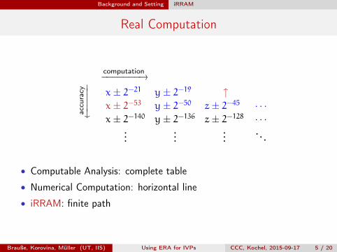
Real Computation
computation−−−−−−−→ac
cura
cy←−−−
−− x± 2−21 y± 2−19 ↑x± 2−53 y± 2−50 z± 2−45 · · ·x± 2−140 y± 2−136 z± 2−128 · · ·
......
.... . .
• Computable Analysis: complete table
• Numerical Computation: horizontal line
• iRRAM: finite path
Brauße, Korovina, Müller (UT, IIS) Using ERA for IVPs CCC, Kochel, 2015-09-17 5 / 20

Background and Setting iRRAM
Real Computation
computation−−−−−−−→ac
cura
cy←−−−
−− x± 2−21 y± 2−19 ↑x± 2−53 y± 2−50 z± 2−45 · · ·x± 2−140 y± 2−136 z± 2−128 · · ·
......
.... . .
• Computable Analysis: complete table
• Numerical Computation: horizontal line
• iRRAM: finite path
Brauße, Korovina, Müller (UT, IIS) Using ERA for IVPs CCC, Kochel, 2015-09-17 5 / 20

Background and Setting Polynomial ODE systems
Polynomial ODE system
d-dimensional polynomial ~f : R×Rd → Rd in d+ 1 variables, then solution~y : R→ Rd described by ODE system
ddt
~y(t) = ~f(t,~y(t))
Usually we also have an initial value ~y0 = ~y(t0) at some t0.
• virtually all real-world ODE systems are describable by poly right handside ~f
• example systems: Van-der-Pol oscillator, n-Body problem, doublependulum, Lorentz attractor, . . .
Brauße, Korovina, Müller (UT, IIS) Using ERA for IVPs CCC, Kochel, 2015-09-17 6 / 20
Background and Setting Polynomial ODE systems
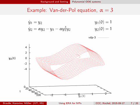
Example: Van-der-Pol equation, α = 3
y1 = y2 y1(0) = 1
y2 = αy2 − y1 − αy21y2 y2(0) = 1
020406080100 -2 -1 0 1 2
-4
-2
0
2
4
y2(t)
vdp-3
t
y1(t)
y2(t)
Brauße, Korovina, Müller (UT, IIS) Using ERA for IVPs CCC, Kochel, 2015-09-17 7 / 20

Algorithm
1 Background and Setting
Motivation
iRRAM
2 Algorithm
3 Radius of Convergance
Picard-Lindelöf’s method
Improved by Integrals
Iterative Improvement
4 Countering wrapping effects
Lipschitz bounds reducing wrapping
Taylor Models
5 Future Work and References
Brauße, Korovina, Müller (UT, IIS) Using ERA for IVPs CCC, Kochel, 2015-09-17 8 / 20

Algorithm
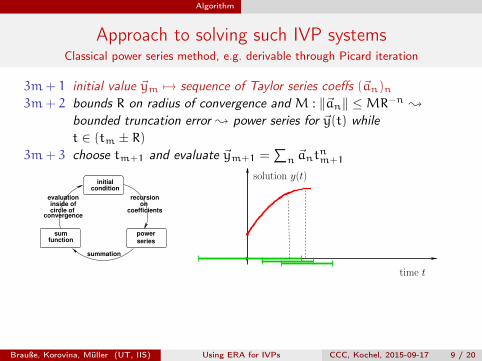
Approach to solving such IVP systemsClassical power series method, e.g. derivable through Picard iteration
3m+ 1 initial value ~ym 7→ sequence of Taylor series coeffs (~an)n3m+ 2 bounds R on radius of convergence and M : ‖~an‖ ≤MR−n ;
bounded truncation error ; power series for ~y(t) whilet ∈ (tm ± R)
3m+ 3 choose tm+1 and evaluate ~ym+1 =∑n ~ant
nm+1
recursionon
coefficients
summation
powerseries
conditioninitial
evaluationinside ofcircle of
convergence
sumfunction
solution y(t)
time t
Good bounds on radius are crucial:
• step size• fewer Taylor series coefficients need to be computed
Brauße, Korovina, Müller (UT, IIS) Using ERA for IVPs CCC, Kochel, 2015-09-17 9 / 20

Algorithm
Approach to solving such IVP systemsClassical power series method, e.g. derivable through Picard iteration
3m+ 1 initial value ~ym 7→ sequence of Taylor series coeffs (~an)n3m+ 2 bounds R on radius of convergence and M : ‖~an‖ ≤MR−n ;
bounded truncation error ; power series for ~y(t) whilet ∈ (tm ± R)
3m+ 3 choose tm+1 and evaluate ~ym+1 =∑n ~ant
nm+1
recursionon
coefficients
summation
powerseries
conditioninitial
evaluationinside ofcircle of
convergence
sumfunction
solution y(t)
time t
Good bounds on radius are crucial:
• step size• fewer Taylor series coefficients need to be computed
Brauße, Korovina, Müller (UT, IIS) Using ERA for IVPs CCC, Kochel, 2015-09-17 9 / 20

Radius of Convergance
1 Background and Setting
Motivation
iRRAM
2 Algorithm
3 Radius of Convergance
Picard-Lindelöf’s method
Improved by Integrals
Iterative Improvement
4 Countering wrapping effects
Lipschitz bounds reducing wrapping
Taylor Models
5 Future Work and References
Brauße, Korovina, Müller (UT, IIS) Using ERA for IVPs CCC, Kochel, 2015-09-17 10 / 20

Radius of Convergance Picard-Lindelöf’s method
Original approach by P-L
Fix some δ and select compact region aroundinitial value:
Cε = {(t0 + t, ~w0 + ~w) : |t| ≤ δ∧ ‖~w‖ ≤ ε}
p(ε) = max ‖f(Cε)‖; RPL(ε) = min{δ, ε/p(ε)}Leaves option to choose ε. . .
δ
R
ε
~w0
t0
p(ε)
020406080100 -2 -1 0 1 2
-4
-2
0
2
4
y2(t)
vdp-3
t
y1(t)
y2(t)
0
0.2
0.4
11 13 15 17
Brauße, Korovina, Müller (UT, IIS) Using ERA for IVPs CCC, Kochel, 2015-09-17 11 / 20

Radius of Convergance Improved by Integrals
p(ε) monotonically increasing ;∫ε01/p(s)ds ≥ ε/p(ε)
Worst-case is on the boundary. So Rint(0, ε) = min{δ,∫ε0 1/p(s)ds}.
RPL Rint
t0
~w0
ε
δ
0
0.2
0.4
11 13 15 17
Brauße, Korovina, Müller (UT, IIS) Using ERA for IVPs CCC, Kochel, 2015-09-17 12 / 20

Radius of Convergance Improved by Integrals
p(ε) monotonically increasing ;∫ε01/p(s)ds ≥ ε/p(ε)
Worst-case is on the boundary. So Rint(0, ε) = min{δ,∫ε0 1/p(s)ds}.
RPL Rint
t0
~w0
ε
δ
0
0.2
0.4
11 13 15 17
Brauße, Korovina, Müller (UT, IIS) Using ERA for IVPs CCC, Kochel, 2015-09-17 12 / 20

Radius of Convergance Improved by Integrals
p(ε) monotonically increasing ;∫ε01/p(s)ds ≥ ε/p(ε)
Worst-case is on the boundary. So Rint(0, ε) = min{δ,∫ε0 1/p(s)ds}.
RPL Rint
t0
~w0
ε
δ
0
0.2
0.4
11 13 15 17Brauße, Korovina, Müller (UT, IIS) Using ERA for IVPs CCC, Kochel, 2015-09-17 12 / 20

Radius of Convergance Iterative Improvement
Have some R
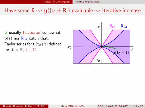
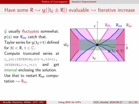
; y([t0 ± R]) evaluable ; Iterative increase
~y usually fluctuates somewhat.p(s) nor Rint catch that.Taylor series for y(t0+t) definedfor |t| < R, t ∈ C.
Compute truncated series atc_int(INTERVAL(t0-t,t0+t),
INTERVAL(-t,+t)) and getinterval enclosing the solution.
Use that to restart Rint compu-tation ; Ritr.
RPL Rint
y(t0 + t)
Ritr
t0
~w0
ε
δ
0
0.2
0.4
11 13 15 17
Brauße, Korovina, Müller (UT, IIS) Using ERA for IVPs CCC, Kochel, 2015-09-17 13 / 20

Radius of Convergance Iterative Improvement
Have some R ; y([t0 ± R]) evaluable
; Iterative increase
~y usually fluctuates somewhat.p(s) nor Rint catch that.Taylor series for y(t0+t) definedfor |t| < R, t ∈ C.
Compute truncated series atc_int(INTERVAL(t0-t,t0+t),
INTERVAL(-t,+t)) and getinterval enclosing the solution.
Use that to restart Rint compu-tation ; Ritr.
RPL Rint
y(t0 + t)
Ritr
t0
~w0
ε
δ
0
0.2
0.4
11 13 15 17
Brauße, Korovina, Müller (UT, IIS) Using ERA for IVPs CCC, Kochel, 2015-09-17 13 / 20
Radius of Convergance Iterative Improvement
Have some R ; y([t0 ± R]) evaluable ; Iterative increase
~y usually fluctuates somewhat.p(s) nor Rint catch that.Taylor series for y(t0+t) definedfor |t| < R, t ∈ C.
Compute truncated series atc_int(INTERVAL(t0-t,t0+t),
INTERVAL(-t,+t)) and getinterval enclosing the solution.
Use that to restart Rint compu-tation ; Ritr.
RPL Rint
y(t0 + t)
Ritr
t0
~w0
ε
δ
0
0.2
0.4
11 13 15 17
Brauße, Korovina, Müller (UT, IIS) Using ERA for IVPs CCC, Kochel, 2015-09-17 13 / 20

Radius of Convergance Iterative Improvement
Have some R ; y([t0 ± R]) evaluable ; Iterative increase
~y usually fluctuates somewhat.p(s) nor Rint catch that.Taylor series for y(t0+t) definedfor |t| < R, t ∈ C.Compute truncated series atc_int(INTERVAL(t0-t,t0+t),
INTERVAL(-t,+t)) and getinterval enclosing the solution.
Use that to restart Rint compu-tation ; Ritr.
RPL Rint
y(t0 + t)
Ritr
t0
~w0
ε
δ
0
0.2
0.4
11 13 15 17
Brauße, Korovina, Müller (UT, IIS) Using ERA for IVPs CCC, Kochel, 2015-09-17 13 / 20
Radius of Convergance Iterative Improvement
Have some R ; y([t0 ± R]) evaluable ; Iterative increase
~y usually fluctuates somewhat.p(s) nor Rint catch that.Taylor series for y(t0+t) definedfor |t| < R, t ∈ C.Compute truncated series atc_int(INTERVAL(t0-t,t0+t),
INTERVAL(-t,+t)) and getinterval enclosing the solution.Use that to restart Rint compu-tation ; Ritr.
RPL Rint
y(t0 + t)
Ritr
t0
~w0
ε
δ
0
0.2
0.4
11 13 15 17
Brauße, Korovina, Müller (UT, IIS) Using ERA for IVPs CCC, Kochel, 2015-09-17 13 / 20

Countering wrapping effects
1 Background and Setting
Motivation
iRRAM
2 Algorithm
3 Radius of Convergance
Picard-Lindelöf’s method
Improved by Integrals
Iterative Improvement
4 Countering wrapping effects
Lipschitz bounds reducing wrapping
Taylor Models
5 Future Work and References
Brauße, Korovina, Müller (UT, IIS) Using ERA for IVPs CCC, Kochel, 2015-09-17 14 / 20
Countering wrapping effects Lipschitz bounds reducing wrapping
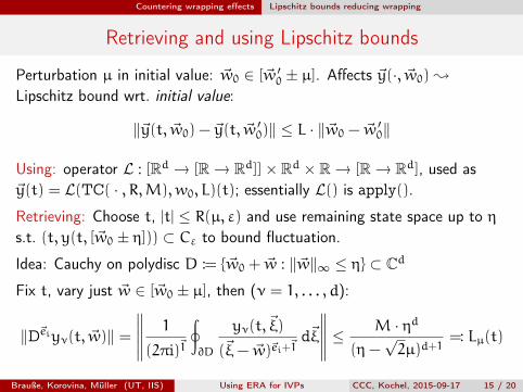
Retrieving and using Lipschitz bounds
Perturbation µ in initial value: ~w0 ∈ [~w ′0 ± µ]. Affects ~y(·, ~w0) ;
Lipschitz bound wrt. initial value:
‖~y(t, ~w0) − ~y(t, ~w ′0)‖ ≤ L · ‖~w0 − ~w ′
0‖
Using: operator L : [Rd → [R→ Rd]]× Rd × R→ [R→ Rd], used as~y(t) = L(TC( · , R,M), w0, L)(t); essentially L() is apply().Retrieving: Choose t, |t| ≤ R(µ, ε) and use remaining state space up to ηs.t. (t, y(t, [~w0 ± η])) ⊂ Cε to bound fluctuation.
Idea: Cauchy on polydisc D := {~w0 + ~w : ‖~w‖∞ ≤ η} ⊂ Cd
Fix t, vary just ~w ∈ [~w0 ± µ], then (ν = 1, . . . , d):
‖D~eiyν(t, ~w)‖ =
∥∥∥∥∥ 1
(2πi)~1
∮∂D
yν(t,~ξ)
(~ξ− ~w)~ei+~1d~ξ
∥∥∥∥∥ ≤ M · ηd
(η−√2µ)d+1
=: Lµ(t)
Brauße, Korovina, Müller (UT, IIS) Using ERA for IVPs CCC, Kochel, 2015-09-17 15 / 20

Countering wrapping effects Taylor Models
Taylor Models
Classic version by Makino/Berz, named wrt. Taylor expansion of functions.
T(~λ) =∑
~n c~n~λ~n polynomial in vector of error variables ~λ ∈ Ik plus a real
remainder interval I; c~n ∈ R
• Representation of real intervals: ∃λ : T(λ) 3 x• Allows for cancellation: T, T ′ both represent x=⇒ T(~λ) − T ′(~λ) = I− I ′ ≈ 0Usual interval arithmetic for I− I ′, though
Generalization: c~n ⊆ R intervals, no remainder interval necessary
• Allows transparent change of representation T 7→ T (“polish”)Example: order reduction: c2,1λ21λ2 ; c2,1I2︸ ︷︷ ︸
c0,1
λ2
• Naturally implementable by types REAL or INTERVAL in iRRAM• Integrate seamlessly to Taylor series evaluation: truncation error 7→ c0
Brauße, Korovina, Müller (UT, IIS) Using ERA for IVPs CCC, Kochel, 2015-09-17 16 / 20

Countering wrapping effects Back to Van-der-Pol example, α = 3
TMs allow to catch rapid convergance near attractorVan-der-Pol, α = 3, different “polishing” strategies
-200
-180
-160
-140
-120
-100
-80
-60
0 2000 4000 6000 8000 10000 12000 14000
Precision
Steps
Brauße, Korovina, Müller (UT, IIS) Using ERA for IVPs CCC, Kochel, 2015-09-17 17 / 20

Countering wrapping effects Back to Van-der-Pol example, α = 3
Timings
method tend steps time initial final bits /[s] precision tend
Lipschitz 10 139 131 2−601 2−100 51.1
20 285 655 2−1151 2−94 52.8
50 – – – – –100 – – – – –
Taylor 10 139 37 2−207 2−190 1.7
model, 20 285 71 2−207 2−179 1.4
older sweep 50 711 180 2−207 2−174 0.62
100 1440 344 2−207 2−156 0.51
Brauße, Korovina, Müller (UT, IIS) Using ERA for IVPs CCC, Kochel, 2015-09-17 18 / 20

Future Work and References
1 Background and Setting
Motivation
iRRAM
2 Algorithm
3 Radius of Convergance
Picard-Lindelöf’s method
Improved by Integrals
Iterative Improvement
4 Countering wrapping effects
Lipschitz bounds reducing wrapping
Taylor Models
5 Future Work and References
Brauße, Korovina, Müller (UT, IIS) Using ERA for IVPs CCC, Kochel, 2015-09-17 19 / 20

Future Work and References
Improve speed of IVP-Solver to match double precision implementations.
Generalize PIVP-Solver to HIVP-Solver w/ H = holom. fns w/ additionallyprovided comp. modulus of continuity
Radius of Convergance:
• Use higher-order TMs to get better approx. for derivatives.• Refine computation towards tighter bounds than Ritr.
Taylor Models:
• Allow to catch attractors ; need better polishing heuristics.• Formalize TMs to reason about behaviour in ERA setting.• Generalize iRRAM’s methods to TMs (and other representationsbesides τTM?); What properties are necessary to enable efficient handling?
iRRAM Documentation: http://irram.uni-trier.de/
iRRAM Code: https://github.com/norbert-mueller/iRRAM
Brauße, Korovina, Müller (UT, IIS) Using ERA for IVPs CCC, Kochel, 2015-09-17 20 / 20