on-line mobile robot model identiﬁcation using integrated

On-line Mobile Robot Model Identification usingIntegrated Perturbative Dynamics

Forrest Rogers-Marcovitz and Alonzo Kelly

Abstract We present an approach to the problem of real-time identification of vehi-cle motion models based on fitting, on a continuous basis, parametrized slip mod-els to observed behavior. Our approach is unique in that we generate parametricmodels capturing the dynamics of systematic error (i.e. slip) and then predict tra-jectories for arbitrary inputs on arbitrary terrain. The integrated error dynamics arelinearized with respect to the unknown parameters to produce an observer relatingerrors in predicted slip to errors in the parameters. An Extended Kalman filter isused to identify this model on-line. The filter forms innovations based on residualdifferences between the motion originally predicted using the present model and themotion ultimately experienced by the vehicle. Our results show that the models con-verge in a few seconds and they reduce prediction error for even benign maneuverswhere errors might be expected to be small already. Results are presented for both askid-steered and an Ackerman steer vehicle.

1 Introduction

Autonomous vehicle research has continuously demonstrated that a platform’s pre-cise understanding of its own mobility is a key ingredient of competent machinesthat perform [4]. Since ground vehicles are propelled over the earth by the twoforces of gravity and traction, agile autonomous mobility relies fundamentally onunderstanding and exploiting the interactions between the terrain and tractive de-vices like wheels and tracks. Furthermore the propulsive forces depend critically onthe composition of the surface over which the vehicle moves. Therefore, unless theterrain is homogeneous for the duration of an entire mission, and the vehicle modelsare already well calibrated, we must conclude that a capacity to calibrate (i.e. iden-tify) vehicle models in real-time is a core requirement of high performance ground

Forrest Rogers-Marcovitz and Alonzo KellyRobotics Institute, Carnegie Mellon University, e-mail: {forrest,alonzo}@cmu.edu

1

2 Forrest Rogers-Marcovitz and Alonzo Kelly

robots. In principle, it should be possible to calibrate vehicle models in real-timebased on observing residual differences between the motion originally predicted bythe platform and the motion ultimately experienced. In a machine learning context,this process would be called self-supervised learning whereas in the adaptive controlcommunity it would be called on-line identification.

We concentrate on the problem of calibrating the faster-than-real-time modelswhich occur in mobile robotic predictive control and motion planning. Such casesinclude obstacle avoidance and path following situations where the predicted motionof the vehicle is the basis for decisions on where to go. Our models calibrate themapping between the control inputs and predicted state trajectory. Certainly thismapping depends on terrain conditions, gravity, reaction and inertial forces but wehave found it unnecessary to express forces explicitly in the models. Our modelsnonetheless provide a fairly accurate model of the underlying dynamics over theregime of performance of present-day robots.

Motion models of ground robots have many uses. Model-based approaches havebeen applied to estimate longitudinal wheel slip and to detect immobilization ofmobile robots [10]. Analytical models also exist for steering maneuvers of planetaryrovers on loose soil [3]. The aspects of wheel-terrain interaction that are needed foraccurate models are neither well known nor easily measurable in realistic situations.Other researchers have addressed the problem of model identification for groundrobots. Algorithms have been developed to learn soil parameters given wheel-terraindynamic models [8].

Our colleagues have constructed an artificial neural network that was used tolearn a forward predictive model of the Crusher Unmanned Ground Vehicle [2]. Thismodel gave good results, with fast predictions, without making any assumptionsabout the vehicle to ground interaction. It was trained off-line and does not attemptto adapt to varying terrain properties.

Whereas published methods are designed to use measurements to estimate presentstate for feedback controllers, our method learns a predictive model by capturing theunderlying dynamics as a function of all of input space. Some published methodslump all of the unknown soil parameters into slip ratios and a slip angle and usevelocity measurements to aid in estimation. An Extended Kalman Filter (EKF) anda Sliding Mode Observer (SMO) have been developed to estimate the slip ratio pa-rameters by [11] and [5]. An EKF has also been used to estimate the slip angles andlongitudinal slippage for a wheeled mobile robot [6].

Our method also relies on more reliable pose residuals rather than measurementsof velocity. In our past work, we have developed off-line calibration techniques [1]including techniques for learning vehicle slip rates [7]. In this paper, we extendthose techniques to work for real time calibration. We first develop a general landvehicle model in Section 2. This model, along with the pose residual observations,is integrated into the EKF in Section 3. Section 4 describes the experimental set-up,and the results are presented in Section 5. We present our conclusions in Section 6.

On-line Mobile Robot Model Identification using Integrated Perturbative Dynamics 3

2 Vehicle Model

For any vehicle moving in contact with a surface, there are three degrees of freedomof in-plane motion as long as the vehicle remains in contact with the terrain, (Figure1). Errors in motion prediction can therefore be reduced, without loss of generality,to instantaneous values of forward slip rate, δVx, side slip rate, δVy, and angular sliprate, δω .

Fig. 1 Vehicle Dynamics.

Given these slip rates and the vehicle’s commanded linear and angular velocity,we have the following kinematic differential equation for the time derivatives of thevehicle’s 2D position and heading with respect to a ground fixed frame of reference,known hereafter as the world frame. x

yθ

=

cθ −sθ 0sθ cθ 00 0 1

Vx

Vyω

+

δVxδVyδω

(1)

cθ = cos(θ), sθ = sin(θ)

This model is the general case for a vehicle moving on a surface with three de-grees of velocity freedom. We expressed the velocity in terms of a commandedcomponent and an error component. Both are expressed in body coordinates be-cause slip is likely to be simpler to express in these coordinates. The model is alsorelevant to rough terrain when expressed in body coordinates because the instan-taneous linear velocity remains in the plane containing the wheel contact points.Ignoring suspension deflections, this plane is fixed in body coordinates. No non-holonomic constraints are present in the unperturbed model above, but they can beeasily added. The perturbations, of course, are elements that will not respect suchconstraints even if they nominally exist. In plain terms, if the wheels are slippingsideways, the perturbations will tell us that.

We elected to use a velocity driven model because these are natural inputs formost of our robots. However, this is not a requirement of our approach. Any dif-ferential equation, such as one driven by forces or fuel flow rates, could be used.It is important to express the model in terms of control inputs rather than measure-


ments since the model will be used to predict motion before the terrain is traversed.Furthermore, the perturbation terms need not be in input space. They could be ex-pressed as additive errors to the state δx or even the state derivatives δ x. They needonly span the dimensions necessary to characterize the actual errors of interest.

The calibration question is how best to model the perturbations. They will de-pend, in general, on terrain composition and vehicle state along with the applied,constraint, and inertial forces that terrain and vehicle state imply. We can param-eterize a 3 × 1 vector of the slip velocity δu, expressed as δu(u, p). These slipvelocities depend, in our model, on the commanded velocities u(Vx,Vy,ω) and on aset of learned slip parameters, p. Accordingly, the perturbed system dynamics canbe written in general as:

x = f (x,u, p) (2)

The use of wheel rotational velocities, or integrals involving them, to form ob-servations is not desirable since such measurements cannot observe slip directly.In addition, wheels may slip sideways and such motion would not be reflected inmeasurements of wheel rotations, even though it is the dominant effect of interest inmany cases. Although many approaches to system identification are based on fittingthe data to the differential equation, we prefer to exploit the high relative accuracyof position data (e.g. RTK GPS or visual odometry) by observing the effects of theslip velocities on the integrated dynamics. This formulation also allows the positionmeasurements to be under-sampled relative to the command frequency; for exam-ple, low-cost GPS may only provide an position update at 1 Hz while the vehicleis commanded at 100 Hz. The vehicle path is found by integrating the equations ofmotion.

x =

xyθ

= F(u(t), p) =∫

f (x(t),u(t), p)dt (3)

In order to produce regular observations, we reset the integral to a local originbefore using the current estimate of slip parameters to produce the difference be-tween measured and predicted changes in pose for a given path segment. To avoida double delta symbol in the notation, let us define the uppercase vector X to be thedifference between two states expressed in ground fixed coordinates:

X(k) = x(tk +n)− x(tk) (4)

This gives us an integrated observation.

∆X = Xmeasured−X predicted (5)


3 Extended Kalman Filter

Any vehicle’s performance will depend on terrain characteristics which vary overspace and time due to such effects as weather and seasonal vegetation. Only an on-line system can adapt to these changes as fast as the local environment changes dur-ing the vehicle’s motion from place to place. In an operational setting, the trajectoryfollowed by the robot will not normally be chosen to simplify model identification.In any case, there is no clear way to tell when the terrain is about to change so thesystem must be able calibrate on any arbitrary trajectory.

An Extended Kalman Filter (EKF) is used whose state vector is composed en-tirely of the parameters governing perturbative (i.e. slip) velocity. The vehicle poseestimation system functions as a sensor for the identification filter. It may use itsown Kalman filter but in this paper the EKF will always mean the identificationEKF used to identify slip parameters. In the EKF, uncertainty in both states (pa-rameters) and the measurements is correctly treated. The transition and observationmodels below are used in the standard EKF algorithm.

3.1 Transition model

Our parameters are assumed to be constant over a short segment once the terrain andthe inputs are known. Therefore, the state transition model is adequately modeledas static in (6). The process noise, ε t , of covariance Qt describes the parameteruncertainty. The uncertainty models can be adaptive, allowing the noise amplitudeto be increased, for example, during terrain transitions that are detected (from rapidchanges in slip) or predicted (from perception). The transition matrix is simply theidentity matrix, (7), so it does not appear in the transition model.

pt = g(pt−1)+ ε t = pt−1 + ε t (6)

Gt =∂g(pt−1)

∂ pt

= I5,5 (IdentityMatrix) (7)

3.2 Observation Model

Each computation of the motion prediction dynamics integral (3) is called a pathsegment. The observation is the measured relative pose between the start and endof the current path segment, Xmeasured , whereas the predictive measurement is thesame quantity as predicted by the current parameter estimates and the sequence ofcommands issued over the segment, (8). The observation noise, δ t , is the expected


noise of the difference between start and end poses, with covariance Rt . More detailon the observation noise is presented in Section 3.3.

zt = h(u(t), pt)+δ t (8)

zt = Xmeasured (9)h(u(t), pt) = X predicted = F(u(t), pt) (10)

Given an observed difference between the predicted and measured relative poseof a path segment, the measurement Jacobian, H, allows us to find the changesneeded in the slip parameters to correct the relative pose residual. Since pose is only3D in the plane and any sophisticated model will have many parameters, we havean under determined system. Optimal estimation, via the Kalman gain, can computechanges in n parameters to correspond to 3 pose residual errors, (11).

∆ p = K∆X = PHT [HPHT +R]−1∆X (11)

The Jacobian, H, which linearizes the change in the integrand F due to the changein parameters p, can be evaluated on an arbitrary trajectory in (12).

H =∂F∂ p

=∂

∂ p

∫f (x(t),u(t), p)dt =

∫∂

∂ pf (x(t),u(t), p)dt (12)

The last step in (12) uses Leibniz’s rule to convert the derivative of the integral tothe integral of the derivative. Numerical finite differences on the integral could alsobe performed, but Leibniz’ rule gives a closed form solution for our formulation.The chain rule is used for the inner derivative to simplify the analytical differentia-tion, (13).

∂ f∂ p

=∂ f

∂δu∂δu∂ p

(13)

The first needed derivative, describing the change in predicted motion relative tothe change in slip rates, is simply the rotation matrix in the motion model.

∂ f∂δu

=

cθ −sθ 0sθ cθ 00 0 1

(14)

Slip rate is represented as a second order polynomial surface over input space.This approach allows us to learn, not only the present slip, but a model for how slipdepends on arbitrary inputs - even arbitrary functions of time. The polynomial termsare formed over commanded speed V , and angular velocity is dropped from thecommand vector in favor of curvature, κ . The result of these formulation decisionsis a slip surface that is a general paraboloid over this input space.


δVx = α1,x κ +α2,xV +α3,x κV +α4,x κ2 +α5,xV 2

δVy = α1,y κ +α2,yV +α3,y κV +α4,y κ2 +α5,yV 2 (15)

δVω = α1,ω κ +α2,ωV +α3,ω κV +α4,ω κ2 +α5,ωV 2

Constant terms were not used since they cause phantom drift when the vehicle is,in fact, not moving. Commanded side velocity was not considered as our vehicles(skid-steered and Ackerman-steered) have no commanded side velocity. Gravity,expressed in the body frame, would likely be needed in the model for slopes, but wehave not performed such experiments yet. Additional terms may be added for otherrelevant inputs, disturbances, or state variables.

Ideally, the inputs used should be whatever the system actually accepts as inputsat the level of abstraction that is being calibrated. For example, one could calibratea decoupled model of a Mars rover which accepts 4 wheel velocities or a state spacemodel of the same system that presents a curvature-accelerator interface like anautomobile.

The slip rate surface parameters are grouped into a column vector to form the 21state vector of the EKF. Equation (16) gives the second needed derivative used ininner derivative, (13).

p = [α1,x α2,x α3,x α4,x α5,x α1,y α2,y α3,y α4,y α5,yα1,ω α2,ω α3,ω α4,ω α5,ω ]>

∂δu∂ p

= U =

C 01,5 01,501,5 C 01,501,5 01,5 C

(16)

C =[κ, V, κV, κ2, V 2

]

3.3 Uncertainty

Given the EKF observation residual, (17), the observation uncertainty is a combi-nation of the measurement uncertainties of the initial and final state plus the un-certainty in the integrand, F, which depends on both the initial pose and parameteruncertainties, (18). Equation (18) assumes that the two pose measurements are un-correlated - which we find to be an adequate model for RTK GPS. For systems thatuse WAAS, or lower grade GPS, a model of the correlation of the two relative poseerrors can be used. GPS errors are of course not white or Gaussian, but a simplecheck such as a validation gate should be able to detect large GPS jumps and re-ject any such measurements. Good inertial navigation systems or visual odometryare likely to be better solutions than GPS since they exhibit excellent short termaccuracy that can observe wheel slip.

∆z = z−h(p) = x f − xi−F(xi, p,u fi ) (17)

Rz = Rx f +Rxi +RF (18)


RF = RFxi+RFp = JxiRxiJ

>xi

+ JpRpJ>p (19)

In estimating the uncertainty in X predicted , it is very important to correctly accountfor the fact that the predicted relative pose error can be caused by a combination oferrors in the initial conditions and errors in the parameters used in the integral. Thatis, a lateral pose error could be caused simply by an error in the yaw angle used asinitial conditions.

The second term in (19) describes the uncertainty in the predicted relative posedue to errors in the slip parameters. We can take the parameter uncertainty and it’sJacobian straight from the EKF; thus Jp = H in (12) and Rp = P, the parametercovariance, in (11).

The first term in (19) describes the uncertainty in the predicted relative pose dueto error in the measured initial pose. The pose measurement uncertainty providedby the position estimation system is used for this. For the Jacobian, the partial insidethe integrand is taken with respect to the initial state rather than the current state ateach point in time as the integral in computed.

Jxi =∂F∂xi

=∂

∂xi

∫f (xi,x, p,u)dt =

∫∂ f (xi,x, p,u)

∂xidt (20)

We can isolate the dependence on the initial angle by rewriting the world-relativeyaw angle, θ , as the sum of the constant initial angle, θi, and the time varyingdeviation from the initial angle, ∆θ(t). This can be represented as a product of tworotation matrices.

f (xi,x, p,u) =

xyθ

=

cθi −sθi 0sθi cθi 00 0 1

c∆θ −s∆θ 0s∆θ c∆θ 0

0 0 1

Vx(p)Vy(p)ω(p)

(21)

The Jacobian is now straightforward since the rotation through the constant initialangle can be taken outside the integral. We define ∆xi

f as the state change expressedin a coordinate system fixed to the initial pose.

∂F(xi, p,u fi )

∂xi=

∂

∂xi


∫ f (x, p,u)dt =∂

∂xi


∗∆xif (22)

The derivative of a matrix with respect to a vector produces a third order tensor(3x3x3) in general. We can simplify this complexity by taking the derivative of therotation matrix with respect to each element of the vector of initial conditions andthen multiplying by the relative pose change, ∆xi

f , to get a single column of theJacobian. First we take the derivative with respect to initial heading.

∂F(xi, p,u fi )

∂θi=

−sθi −cθi 0cθi −sθi 00 0 1

∗∆xif =

−∆y∆x0

(23)


The changes in position produced, ∆x and ∆y, are expressed in world coordi-nates. Because the rotation matrix is independent of the initial position, (xi,yi), theother two columns of the Jacobian are zero. This gives us the final Jacobian:

Jxi =

0 0 −∆y0 0 ∆x0 0 0

(24)

The result is intuitively correct since this is the Jacobian of a rotation of a dis-placement vector rotated through an angle at the start. If we multiply out the wholefirst uncertainty term, we get:

JxiRxiJ>xi

=

∆y2 −∆y∆x 0−∆y∆x ∆x2 0

0 0 0

σθiθi (25)

The uncertainty propagation can be used to estimate the error in trajectory pre-diction for planning purposes. Vehicle motion planners can improve performanceand better avoid obstacles if they know the likely regions occupied by the vehicleafter executing an arbitrary trajectory. The uncertainty in the integrand, RF , foundin Equation (19), gives the uncertainty in the predicted pose from the uncertainty inthe parameters and the uncertainty in the initial state.

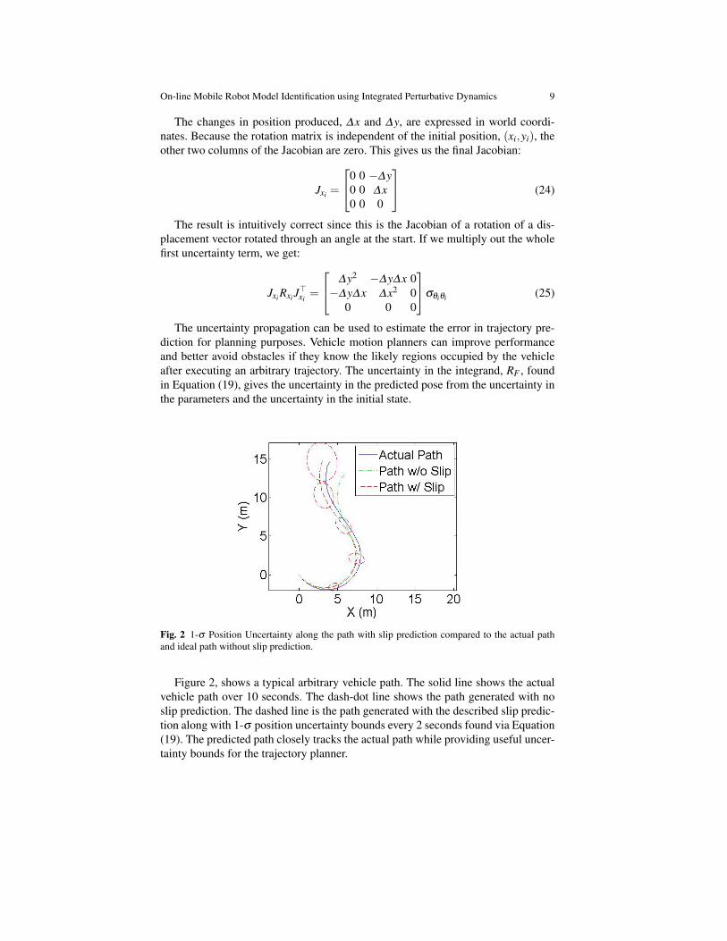
Fig. 2 1-σ Position Uncertainty along the path with slip prediction compared to the actual pathand ideal path without slip prediction.

Figure 2, shows a typical arbitrary vehicle path. The solid line shows the actualvehicle path over 10 seconds. The dash-dot line shows the path generated with noslip prediction. The dashed line is the path generated with the described slip predic-tion along with 1-σ position uncertainty bounds every 2 seconds found via Equation(19). The predicted path closely tracks the actual path while providing useful uncer-tainty bounds for the trajectory planner.


4 Experimental Set-Up

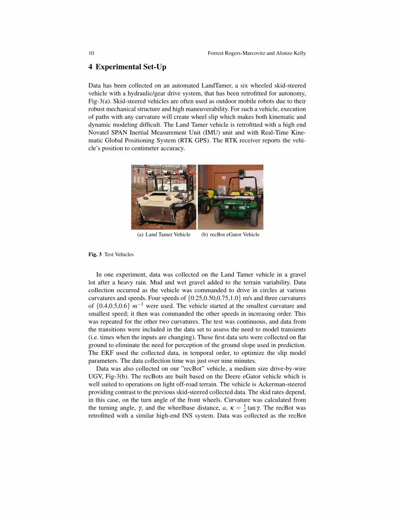
Data has been collected on an automated LandTamer, a six wheeled skid-steeredvehicle with a hydraulic/gear drive system, that has been retrofitted for autonomy,Fig-3(a). Skid-steered vehicles are often used as outdoor mobile robots due to theirrobust mechanical structure and high maneuverability. For such a vehicle, executionof paths with any curvature will create wheel slip which makes both kinematic anddynamic modeling difficult. The Land Tamer vehicle is retrofitted with a high endNovatel SPAN Inertial Measurement Unit (IMU) unit and with Real-Time Kine-matic Global Positioning System (RTK GPS). The RTK receiver reports the vehi-cle’s position to centimeter accuracy.

(a) Land Tamer Vehicle (b) recBot eGator Vehicle

Fig. 3 Test Vehicles

In one experiment, data was collected on the Land Tamer vehicle in a gravellot after a heavy rain. Mud and wet gravel added to the terrain variability. Datacollection occurred as the vehicle was commanded to drive in circles at variouscurvatures and speeds. Four speeds of {0.25,0.50,0.75,1.0}m/s and three curvaturesof {0.4,0.5,0.6} m−1 were used. The vehicle started at the smallest curvature andsmallest speed; it then was commanded the other speeds in increasing order. Thiswas repeated for the other two curvatures. The test was continuous, and data fromthe transitions were included in the data set to assess the need to model transients(i.e. times when the inputs are changing). These first data sets were collected on flatground to eliminate the need for perception of the ground slope used in prediction.The EKF used the collected data, in temporal order, to optimize the slip modelparameters. The data collection time was just over nine minutes.

Data was also collected on our ”recBot” vehicle, a medium size drive-by-wireUGV, Fig-3(b). The recBots are built based on the Deere eGator vehicle which iswell suited to operations on light off-road terrain. The vehicle is Ackerman-steeredproviding contrast to the previous skid-steered collected data. The skid rates depend,in this case, on the turn angle of the front wheels. Curvature was calculated fromthe turning angle, γ , and the wheelbase distance, a, κ = 1

a tanγ . The recBot wasretrofitted with a similar high-end INS system. Data was collected as the recBot


was randomly driven around on a grass lawn for just over five and half minutes atspeeds up to 4.8 m/s. The grass was mostly level and flat, although tractor treads inthe ground provided additional variance in the skip rates.

5 Results

Overlapping one-second path segments were used for computing the path residuals.It is significant that residuals were large enough over such a short time period topermit identification of the model despite the sensor noise. Each iteration occurredwith pose measurement updates at 100 Hz; thus, the segment start points were sep-arated by 10 milliseconds. Keeping track of the past internal derivatives, ∂ f /∂ p,along the length of the path segment made the on-line integration very efficient. Theentire EKF algorithm can easily run faster than real-time.

As the EKF was run on the collected Land Tamer circular data, a future path seg-ment is predicted from the current pose with the current estimated slip parameters.The remaining predicted pose residuals from the measured end pose were minimalwith a few exceptions during transients (perhaps due to un-modeled actuation de-lays), Figure 4(b). For comparison, the relative pose residuals computed without slipprediction are shown in Figure 4(a).

(a) Pose Residuals without Slip Prediction (b) Pose Residuals with Slip Prediction

Fig. 4 Predicted Pose Residuals, 1 second path segments

Parameter values converge in a few seconds once the vehicle enters a newspeed/curvature regime, and the models are formulated to be valid throughout in-put space. The system cannot distinguish innovations caused by changes in terrainfrom those caused by parameter errors so the net result is to adapt to terrain changesin the same way at the same rate. Stochastic models have also been successfullyidentified in an off-line setting [7] in order to quantify the remaining variation af-ter the systematic model converges. Future work will integrate the stochastic modelinto the EKF for on-line identification.


It is significant that the slip rate surface parameters were all initialized to zero,making no assumptions about the vehicle-ground interaction. This is more evidenceof rapid on-line adaptation to the terrain. The slip surface parameter variation overthe EKF run is shown in Figure 5 versus the algorithm iteration index. The parame-ters are clearly adjusting to incorporate new knowledge when new operating regimesare first encountered.

Fig. 5 Parameter Variation during EKF iterations

The final learned slip rate surfaces for the LandTamer are shown in Figure 6.The surfaces are the final predicted mean slip rates over the observed commandedcurvatures and speeds. The surfaces themselves tell us that lateral slip is nearlynonexistent for such a vehicle and the dominant slip directions are best characterizedas rotational and forward.

Even for the benign conditions in this dataset, the EKF relative position estima-tion over 1 second path segments was two times better than the result obtained withno slip prediction, Table 1. The EKF provides an improvement of ten times reduc-tion in the predicted path residual orientation error over path prediction with no sliprates.

Table 1 Relative Pose Error Comparison with Standard Deviation

Algorithm Position (m) Orientation (rad)None .075± .058 .157± .084EKF .034± .042 .014± .019

The improvements are more pronounced as the path segment length or predic-tion time increases, Figure 7. While the position error for a path segment, with nopredicted slip, increases rapidly as the path time length increases, the EKF position


(a) Forward Slip (b) Side Slip

(c) Angular Slip

Fig. 6 Slip Surfaces learned via EKF

error is increases at a much slower rate. With a path time length of six seconds, wesee a position error improvement from 1.6 meters to under 21 centimeters - an er-ror reduction of over about 8 times. Clearly a motion model for this vehicle on thisterrain can be calibrated, and it can be calibrated well.

Fig. 7 Land Tamer Predicted Position Residual with regard to Path Length


The EKF was also run on the collected RecBot data. Recall this test was per-formed at speeds up to 4.8 m/s and steering inputs were arbitrary. The predictionwas more difficult due to less frequent (10 Hz) pose updates, which affects the pathintegration, and an inaccurate steering wheel angle encoder. In addition, the vehiclewas driven at high speeds through more aggressive maneuvers. While the EKF errorresiduals were not as small, the relative improvements, over not using slip in themotion prediction, are similar to those of the Land Tamer data set. The position er-ror grows rapidly as the path segment length is increased, Figure 8. At six seconds,the position error decreases around 3 times. The other plots for the RecBot are notshown here due to space considerations.

Fig. 8 RecBot Predicted Position Residual with regard to Path Length

6 Conclusion

A method has been developed for real-time identification of vehicle dynamic mod-els. The method uses perturbative models to represent slip in all degrees of free-dom, and the model relates slip velocities to arbitrary input signals. Our residualsare based on pose predictions generated from integrating the model over a short pe-riod of time. Though more complex than classical techniques, the approach permitsthe direct use of high quality sensing like RTK GPS, or even under-sampled posemeasurements, as ground truth. This technique requires the linearization of an inte-gral of the system dynamics with respect to the model parameters. The process isclearly observable over all of input space for our vehicles and it converges in a fewseconds on the tested terrain.

The vehicle motion model is a general formulation that applies to any vehicletype and any terrain. In this paper, we have applied it to both skid-steered andAckerman-steered vehicles on loose gravel and grass. Future work will expand theEKF for rolling terrain, for a range of vehicle types, and for multiple terrain types.In addition, command delay transients will be simultaneously learned. Ultimately,perception based slip prediction will permit vehicle control and motion planningto predict the terrain characteristics based on its previewed geometry and appear-


ance. Our formulation also leads to an equivalent capacity to calibrate a stochasticdynamics model by using the integral of the associated linear variance equation.

Our method improves prediction for a few seconds of trajectory prediction whileadapting rapidly to terrain. The improved models produced by this technique willlead to significant improvements in the performance of model predictive controllers,particularly in difficult terrains or during aggressive maneuvers.

Acknowledgments

This work was supported by the U. S. Army Research Office under contract Real-Time Identification of Wheel Terrain Interaction Models for Enhanced AutonomousVehicle Mobility (contract number W911NF-09-1-0557).

References

1. M. Alarfaj and F. Rogers-Marcovitz, “Interaction of Pose Estimation and Online DynamicModeling for a Small Inspector Spacecraft,” ESA Small Satellites Systems and Services 4SSymposium, Funchal, Madeira, Portugal, May 2010.

2. M. Bode, “Learning the Forward Predictive Model for an Off-Road Skid-Steer Vehicle,” tech.report CMU-RI-TR-07-32, Robotics Institute, Carnegie Mellon University, September, 2007.

3. G. Ishigami, A. Miwa, K. Nagatani, and K. Yoshida, “Terramechanics-Based Model for Steer-ing Maneuver of Planetary Exploration Rovers on Loose Soil,” Journal of Field Robotics, Vol.24, No. 3, March, 2007, pp. 233-250.

4. A. Kelly, A. Stentz, O. Amidi, M. Bode, D. Bradley, A. Diaz-Calderon, M. Happold, H. Her-man, R. Mandelbaum, T. Pilarski, P. Rander, S. Thayer, N. Vallidis, and R. Warner. “TowardReliable Off Road Autonomous Vehicles Operating in Challenging Environments,” The Inter-national Journal of Robotics Research, Vol 25, No 5/6, 2006.

5. E. Lucet, C. Grand, D. Sall, and P. Bidaud, “Dynamic sliding mode control of a four-wheelskid-steering vehicle in presence of sliding”, Romansy, Tokyo, Japan, July 2008.

6. C. B. Low and D. Wang, “Integrated Estimation for Wheeled Mobile Robot posture, velocities,and wheel skidding perturbations,” IEEE International Conference on Robotics and Automa-tion. Rome, Itatly, August 2007.

7. F. Rogers-Marcovitz, “On-line Mobile Robotic Dynamic Modeling using Integrated Perturba-tive Dynamics,” tech. report CMU-RI-TR-10-15, Robotics Institute, Carnegie Mellon Univer-sity, April 2010.

8. L. Seneviratne, Y. Zweiri, S. Hutangkabodee, Z. Song, X. Song, S. Chhaniyara, S. Al-Milli,and K. Althoefer. “The modeling and estimation of driving forces for unmanned ground ve-hicles in outdoor terrain,” International Journal of Modeling, Identification, and Control, Vol.6, No. 1, 2009

9. X. Song, L. D. Seneviratne, K. Althoefer, and Z. Song, “A Robust Slip Estimation Methodfor Skid-Steered Mobile Robots,” Intl. Conf. on Control, Automation, Robotics, and Vision,Hanoi, Vietnam, Dec. 2008

10. C. Ward, and K. Iagnemma, “A Dynamic Model-Based Wheel Slip Detector for MobileRobots on Outdoor Terrain,” IEEE Transactions on Robotics, Vol. 24, No. 4, pp. 821-831,Aug. 2008.

11. J. Yi, H. Wang, J. Zhang, D. Song, S. Jayasuriya, and J. Liu, “Kinematic Modeling and Anal-ysis of Skid-Steered Mobile Robots With Applications to Low-Cost Inertial-Measurement-Unit-Based Motion Estimation,” IEEE Transactions on Robotics, Vol. 25, No. 6, Oct. 2009.

on-line mobile robot model identiﬁcation using integrated

Documents