on-line monitoring and oscillatory stability margin
TRANSCRIPT

On-line Monitoring and Oscillatory Stability
Margin Prediction in Power Systems
Based on System Identification
by
Hassan Ghasemi
A thesis
presented to the University of Waterloo
in fulfilment of the
thesis requirement for the degree of
Doctor of Philosophy
in
Electrical and Computer Engineering
Waterloo, Ontario, Canada, 2006
c© Hassan Ghasemi 2006

I hereby declare that I am the sole author of this thesis. This is a true copy of
the thesis, including any required final revisions, as accepted by my examiners.
I understand that my thesis may be made electronically available to the public.
ii

Abstract
Poorly damped electromechanical modes detection in a power system and corre-
sponding stability margins prediction are very important in power system planning
and operation, and can provide significant help to power system operators with
preventing stability problems.
Stochastic subspace identification is proposed in this thesis as a technique to
extract the critical mode(s) from the measured ambient noise without requiring
artificial disturbances (e.g. a line outage), allowing these critical modes to be used
as an on-line index, which is referred here to as System Identification Stability
Indices (SISI) to predict the closest oscillatory instability. The SISI is not only
independent of system models and truly representative of the actual system, but
also computationally efficient. In addition, readily available signals in a power
system and several identification methods are categorized, and merits and pitfalls
of each one are addressed in this work.
The damping torque of linearized models of power systems is studied in this
thesis as another possible on-line security index. This index is estimated by means
of proper system identification techniques applied to both power system transient
response and ambient noise. The damping torque index is shown to address some
of drawbacks of the SISI.
This thesis also demonstrates the connection between the second order statistical
properties, including confidence intervals, of the estimated electromechanical modes
and the variance of model parameters. These analyses show that Monte-Carlo
type of experiments or simulations can be avoided, hence resulting in a significant
reduction in the number of samples.
In these types of studies, the models available in simulation packages are ex-
iii

tremely important due to their unquestionable impact on modal analysis results.
Hence, in this thesis, the validity of generator subtransient model and a typical
STATCOM transient stability (TS) model are also investigated by means of system
identification, illustrating that under certain conditions the STATCOM TS model
can yield results that are too optimistic, which can lead to errors in power system
planning and operation.
In addition to several small test systems used throughout this thesis, the fea-
sibility of the proposed indices are tested on a realistic system with 14,000 buses,
demonstrating their usefulness in practice.
iv

Acknowledgments
I would like to express my sincere gratitude to Prof. Claudio A. Canizares. I cannot
say enough about his constant support, continuous encouragement and priceless
guidance throughout my PhD study. In short, it was a great honor to work with
him.
I am deeply indebted to Dr. Gordon Savage from System Design Engineering
Department for fruitful, enlightening discussions. His remarkable skills and ex-
pertise were always beneficial to completing different parts of this thesis. Sincere
thanks to Dr. Mehrdad Kazerani for providing technical support for parts of the
research related to FACTS controllers. I will always remember the discussions and
help of Dr. Hamid Sheikhzadeh on signal processing issues.
Warmest thanks to my colleagues in the Powerlab at the University of Waterloo:
Mithulan, Sameh, Federico, Valery, Hong, Hamidreza, Warren, Rafael, Ismael, and
Amirhossein.
The valuable remarks and suggestions from Powertech Labs’ personnel is greatly
appreciated. Special thanks to Dr. Prabha Kundur for providing an internship
opportunity in Powertech Labs, which gave me great experience and a chance to
meet wonderful people.
Very special thanks to my parents for their love and hardships during all years
of my studies. The support and continuous encouragement of my brothers and
sister are greatly acknowledged.
Last but not least, I would like to express my utmost thanks to my dear wife,
Salimeh, for her unwavering support and truly pure love during sunny and cloudy
days.
This thesis is dedicated to my wife and our lovely daughter, Hanyeh.
v

Contents
1 Introduction 1
1.1 Research Motivation . . . . . . . . . . . . . . . . . . . . . . . . . . 1
1.2 Literature Review . . . . . . . . . . . . . . . . . . . . . . . . . . . . 3
1.2.1 Stability Limit Prediction . . . . . . . . . . . . . . . . . . . 3
1.2.2 Electromechanical Mode Detection . . . . . . . . . . . . . . 4
1.2.3 Modeling Effect on Stability Limits . . . . . . . . . . . . . . 5
1.3 Objectives . . . . . . . . . . . . . . . . . . . . . . . . . . . . . . . . 7
1.4 Outline of the Thesis . . . . . . . . . . . . . . . . . . . . . . . . . . 7
2 Background Review 9
2.1 Introduction . . . . . . . . . . . . . . . . . . . . . . . . . . . . . . . 9
2.2 Modeling . . . . . . . . . . . . . . . . . . . . . . . . . . . . . . . . . 9
2.2.1 Generators . . . . . . . . . . . . . . . . . . . . . . . . . . . . 10
2.2.2 Loads . . . . . . . . . . . . . . . . . . . . . . . . . . . . . . 11
2.2.3 Synchronous STATic COMpensator (STATCOM) . . . . . . 12
vi

2.3 Power System Stability . . . . . . . . . . . . . . . . . . . . . . . . . 17
2.3.1 Voltage Stability . . . . . . . . . . . . . . . . . . . . . . . . 18
2.3.2 Angle Stability . . . . . . . . . . . . . . . . . . . . . . . . . 19
2.4 Tools . . . . . . . . . . . . . . . . . . . . . . . . . . . . . . . . . . . 20
2.4.1 Continuation Power Flow . . . . . . . . . . . . . . . . . . . 20
2.4.2 Small-Disturbance Stability Analysis . . . . . . . . . . . . . 21
2.4.3 Time-Domain Simulation . . . . . . . . . . . . . . . . . . . . 22
2.4.4 Identification . . . . . . . . . . . . . . . . . . . . . . . . . . 23
2.5 Test Systems . . . . . . . . . . . . . . . . . . . . . . . . . . . . . . 24
2.5.1 Single-Machine-Infinite-Bus (SMIB) . . . . . . . . . . . . . . 24
2.5.2 IEEE 3-bus System . . . . . . . . . . . . . . . . . . . . . . . 24
2.5.3 IEEE 14-bus System . . . . . . . . . . . . . . . . . . . . . . 25
2.5.4 Two-area Benchmark System . . . . . . . . . . . . . . . . . 25
2.5.5 Real 14,000-bus System . . . . . . . . . . . . . . . . . . . . 27
2.6 Summary . . . . . . . . . . . . . . . . . . . . . . . . . . . . . . . . 28
3 System Identification Techniques 29
3.1 Introduction . . . . . . . . . . . . . . . . . . . . . . . . . . . . . . . 29
3.2 Ringdown Data . . . . . . . . . . . . . . . . . . . . . . . . . . . . . 30
3.2.1 Prony Method . . . . . . . . . . . . . . . . . . . . . . . . . . 30
3.3 Ambient Data . . . . . . . . . . . . . . . . . . . . . . . . . . . . . . 33
3.3.1 ARMA Model . . . . . . . . . . . . . . . . . . . . . . . . . . 34
vii

3.3.2 Parameter Estimation . . . . . . . . . . . . . . . . . . . . . 35
3.3.3 AR Parameter Estimation . . . . . . . . . . . . . . . . . . . 39
3.3.4 Stochastic Subspace Identification . . . . . . . . . . . . . . . 42
3.3.5 Computational Issues . . . . . . . . . . . . . . . . . . . . . . 46
3.4 Summary . . . . . . . . . . . . . . . . . . . . . . . . . . . . . . . . 50
4 System Identification Stability Index 51
4.1 Introduction . . . . . . . . . . . . . . . . . . . . . . . . . . . . . . . 51
4.2 Proposed Oscillatory Stability Index . . . . . . . . . . . . . . . . . 52
4.3 SISI from Transient Response . . . . . . . . . . . . . . . . . . . . . 54
4.3.1 IEEE 3-bus System . . . . . . . . . . . . . . . . . . . . . . . 55
4.3.2 IEEE 14-bus System . . . . . . . . . . . . . . . . . . . . . . 63
4.3.3 Real System (14,000 buses) . . . . . . . . . . . . . . . . . . 66
4.4 SISI from Ambient Data . . . . . . . . . . . . . . . . . . . . . . . . 72
4.4.1 IEEE 14-bus System . . . . . . . . . . . . . . . . . . . . . . 74
4.4.2 Two-Area Benchmark System . . . . . . . . . . . . . . . . . 78
4.5 Summary . . . . . . . . . . . . . . . . . . . . . . . . . . . . . . . . 83
5 Damping Torque Index 84
5.1 Introduction . . . . . . . . . . . . . . . . . . . . . . . . . . . . . . . 84
5.2 Damping and Synchronizing Torque . . . . . . . . . . . . . . . . . . 85
5.2.1 Damping and Synchronizing Coefficients . . . . . . . . . . . 86
viii

5.2.2 Electromechanical Mode Estimation . . . . . . . . . . . . . . 88
5.3 Techniques . . . . . . . . . . . . . . . . . . . . . . . . . . . . . . . . 88
5.3.1 Ordinary Least Square (OLS) . . . . . . . . . . . . . . . . . 88
5.3.2 Generalized Least Square (GLS) . . . . . . . . . . . . . . . 89
5.3.3 Robust Fitting with Bisquare Weights (RFBW) . . . . . . . 90
5.4 Damping Torque Estimation from Transient Response . . . . . . . . 91
5.4.1 Single-Machine-Infinite-Bus (SMIB) . . . . . . . . . . . . . . 92
5.4.2 Two-area Benchmark System . . . . . . . . . . . . . . . . . 92
5.4.3 Real System (14,000 buses) . . . . . . . . . . . . . . . . . . 98
5.5 Damping Torque Estimation from Ambient Data . . . . . . . . . . 102
5.5.1 Box-Jenkins Model . . . . . . . . . . . . . . . . . . . . . . . 102
5.5.2 Two-area Benchmark System-Schedules 1 and 2 . . . . . . . 103
5.6 Summary . . . . . . . . . . . . . . . . . . . . . . . . . . . . . . . . 113
6 Estimation of Uncertainty 114
6.1 Introduction . . . . . . . . . . . . . . . . . . . . . . . . . . . . . . . 114
6.2 Covariance of Parameters . . . . . . . . . . . . . . . . . . . . . . . 115
6.3 Covariance of Eigenvalues . . . . . . . . . . . . . . . . . . . . . . . 118
6.4 Test case . . . . . . . . . . . . . . . . . . . . . . . . . . . . . . . . . 119
6.5 Summary . . . . . . . . . . . . . . . . . . . . . . . . . . . . . . . . 120
ix

7 System Identification Techniques Applied to Model Validation 123
7.1 Introduction . . . . . . . . . . . . . . . . . . . . . . . . . . . . . . . 123
7.2 Generator Modeling . . . . . . . . . . . . . . . . . . . . . . . . . . . 124
7.3 STATCOM Modeling . . . . . . . . . . . . . . . . . . . . . . . . . . 126
7.3.1 Test case . . . . . . . . . . . . . . . . . . . . . . . . . . . . . 127
7.3.2 Standard Control Analysis . . . . . . . . . . . . . . . . . . . 128
7.3.3 Supplementary Control Analysis . . . . . . . . . . . . . . . . 128
7.4 Summary . . . . . . . . . . . . . . . . . . . . . . . . . . . . . . . . 131
8 Conclusions 137
8.1 Summary and Conclusions . . . . . . . . . . . . . . . . . . . . . . . 137
8.2 Contributions . . . . . . . . . . . . . . . . . . . . . . . . . . . . . . 139
8.3 Directions for Future Work . . . . . . . . . . . . . . . . . . . . . . . 141
A SYSTEM DATA 142
A.1 IEEE 3-bus System . . . . . . . . . . . . . . . . . . . . . . . . . . 142
A.2 IEEE 14-bus System . . . . . . . . . . . . . . . . . . . . . . . . . . 145
A.3 Two-area Benchmark System . . . . . . . . . . . . . . . . . . . . . 146
B SISI Proof 149
C Alternative Damping Torque Formulation 151
x

List of Figures
2.1 Basic structure of STATCOM. . . . . . . . . . . . . . . . . . . . . . 14
2.2 STATCOM control block diagram with phase control. . . . . . . . . 15
2.3 STATCOM control block diagram with PWM control. . . . . . . . . 15
2.4 Voltage-Current characteristic of a STATCOM. . . . . . . . . . . . 16
2.5 STATCOM transient stability model and its control [1]. . . . . . . . 17
2.6 A typical PV curve and corresponding SLM and DLM. . . . . . . . 21
2.7 Single-Machine-Infinite-Bus (SMIB). . . . . . . . . . . . . . . . . . 24
2.8 IEEE 3-bus test system. . . . . . . . . . . . . . . . . . . . . . . . . 25
2.9 IEEE 14-bus test system. . . . . . . . . . . . . . . . . . . . . . . . . 26
2.10 Two-area benchmark system. . . . . . . . . . . . . . . . . . . . . . 27
3.1 The performance of YW, MYW, LSMYW, and PEM in electrome-
chanical mode estimation from ambient data. . . . . . . . . . . . . 43
3.2 Standard deviation of the estimated real part α of the inter-area
mode −0.1228 ± j4.7824 for the 2-area benchmark system. . . . . . 48
3.3 Standard deviation of the estimated frequency of the inter-area mode
−0.1228 ± j4.7824 for the 2-area benchmark system. . . . . . . . . 49
xi

4.1 SISI profile for a real power system with varying operating conditions. 55
4.2 P-V curves at Bus 3 for the IEEE 3-bus system, for the base case
and for a line 2-3 outage. . . . . . . . . . . . . . . . . . . . . . . . . 57
4.3 Generator G1 speed following a line 2-3 outage in the IEEE 3-bus
system. . . . . . . . . . . . . . . . . . . . . . . . . . . . . . . . . . . 58
4.4 Eigenvalue profiles with respect to load changes in the IEEE 3-bus
system. . . . . . . . . . . . . . . . . . . . . . . . . . . . . . . . . . . 59
4.5 Stability index for the IEEE 3-bus system for SNR = 30 db; base
system. . . . . . . . . . . . . . . . . . . . . . . . . . . . . . . . . . . 60
4.6 Stability index for the IEEE 3-bus system for SNR = 30 db; line 2-3
outage. . . . . . . . . . . . . . . . . . . . . . . . . . . . . . . . . . . 61
4.7 Stability index for the IEEE 3-bus system for SNR = 10 db; base
system. . . . . . . . . . . . . . . . . . . . . . . . . . . . . . . . . . . 62
4.8 Standard deviation of parameter estimates for the IEEE 3-bus sys-
tem; ai’s are the characteristic equation coefficients. . . . . . . . . . 64
4.9 Standard deviation of the SISI and the critical mode’s frequency for
the IEEE 3-bus system. . . . . . . . . . . . . . . . . . . . . . . . . . 65
4.10 P-V curves for the IEEE 14-bus system at Bus 14, for the base case
and for a line 2-4 outage. . . . . . . . . . . . . . . . . . . . . . . . . 67
4.11 Eigenvalue profiles with respect to load changes in the IEEE 14-bus
system. . . . . . . . . . . . . . . . . . . . . . . . . . . . . . . . . . . 68
4.12 Stability index for the IEEE 14-bus system; base system. . . . . . . 69
4.13 Stability index for the IEEE 14-bus system; line 2-4 outage. . . . . 70
xii
4.14 Generator G2 speed following a three phase fault at Bus 4 in the
IEEE 14-bus system. . . . . . . . . . . . . . . . . . . . . . . . . . . 71
4.15 SISI for the 14,000-bus real system. . . . . . . . . . . . . . . . . . . 73
4.16 Mean of the real part and frequency of the identified critical mode
µc = αc ± βc. . . . . . . . . . . . . . . . . . . . . . . . . . . . . . . 75
4.17 Standard deviation of the real part and frequency of the identified
critical mode µc = αc ± βc. . . . . . . . . . . . . . . . . . . . . . . . 76
4.18 Singular values of weighted projection (3.26). . . . . . . . . . . . . . 77
4.19 One-minute block measurement of the change in generator G2’s power
at a 285 MW loading level. . . . . . . . . . . . . . . . . . . . . . . . 79
4.20 SISI for the IEEE 14-bus system obtained with the use of the sub-
space method. . . . . . . . . . . . . . . . . . . . . . . . . . . . . . . 80
4.21 P-V curve at Bus 11 for the 2-area benchmark system. . . . . . . . 81
4.22 SISI for the 2-area benchmark system obtained with use of the sub-
space method. . . . . . . . . . . . . . . . . . . . . . . . . . . . . . . 82
5.1 Torque-speed block diagram. . . . . . . . . . . . . . . . . . . . . . . 87
5.2 Damping coefficient Kd from transient response for the SMIB. . . . 93
5.3 Eigenvalue profiles for different dispatch scenarios; Schedules 1 and 2. 95
5.4 P-V curves at Bus 7 for the 2-area benchmark system. . . . . . . . 96
5.5 Damping coefficients of all generators obtained from transient re-
sponse for the 2-area benchmark system for Schedule 1. . . . . . . . 97
5.6 Damping coefficients of all generators obtained from transient re-
sponse for the 2-area benchmark system for Schedule 2. . . . . . . . 99
xiii

5.7 Generator speed oscillations due to the trigger of the unstable elec-
tromechanical mode in the 14,000-bus real system. . . . . . . . . . . 100
5.8 Damping coefficients of slack generators in different areas for the
14,000-bus real system. . . . . . . . . . . . . . . . . . . . . . . . . . 101
5.9 Loss function for the BJ(nc,nd) model in the 2-area benchmark sys-
tem; Schedule 1. . . . . . . . . . . . . . . . . . . . . . . . . . . . . . 105
5.10 Loss function for the BJ(nc,nd) in the 2-area benchmark system;
Schedule 2. . . . . . . . . . . . . . . . . . . . . . . . . . . . . . . . 106
5.11 Whiteness test for the OLS and BJ(1,2) models using ACF(ǫ[k]) in
the 2-area benchmark system; Schedule 1. Horizontal bars indicate
95% confidence intervals. . . . . . . . . . . . . . . . . . . . . . . . . 107
5.12 Whiteness test for the OLS and BJ(2,5) models using ACF(ǫ[k]) in
the 2-area benchmark system; Schedule 2. Horizontal bars indicate
95% confidence intervals. . . . . . . . . . . . . . . . . . . . . . . . . 108
5.13 The standard deviation of estimated Kd and Ks for the BJ(nc,nd)
model; Schedule 1. . . . . . . . . . . . . . . . . . . . . . . . . . . . 109
5.14 Damping coefficients of all generators from ambient data for the 2-
area benchmark system; Schedule 1. . . . . . . . . . . . . . . . . . . 111
5.15 Damping coefficients of all generators from ambient data for the 2-
area benchmark system; Schedule 2. . . . . . . . . . . . . . . . . . . 112
6.1 Standard deviation of the real part of the identified critical mode
−0.1228 ± j4.7824 for the 2-area benchmark system using Monte-
Carlo and equation (6.18). . . . . . . . . . . . . . . . . . . . . . . . 121
xiv

6.2 Standard deviation of the frequency of the identified critical mode
−0.1228 ± j4.7824 for the 2-area benchmark system using Monte-
Carlo and equation (6.18). . . . . . . . . . . . . . . . . . . . . . . . 122
7.1 SISI for the IEEE 3-bus system; generator detailed model versus its
subtransient model. . . . . . . . . . . . . . . . . . . . . . . . . . . . 125
7.2 The response of the system to a line 2-3 outage in the IEEE 3-bus
system; STATCOM at Bus 3 without supplementary control at 160%
loading level. . . . . . . . . . . . . . . . . . . . . . . . . . . . . . . 129
7.3 Detailed STATCOM model with and without a supplementary con-
trol at a 130% loading level. . . . . . . . . . . . . . . . . . . . . . . 132
7.4 IEEE 3-bus system response for a line 2-3 outage for a STATCOM
with a supplementary control at 190% loading level. . . . . . . . . . 133
7.5 IEEE 3-bus system response for a line 2-3 outage for a STATCOM
with a supplementary control at a 190% loading level. . . . . . . . . 134
7.6 The active and reactive power absorbed by the STATCOM with a
supplementary control at a 190% loading level. . . . . . . . . . . . . 135
xv

List of Tables
3.1 CPU time in seconds for different methods and system orders . . . 47
7.1 Effect of including/neglecting network transients on the critical mode 126
7.2 STATCOM static data . . . . . . . . . . . . . . . . . . . . . . . . . 127
7.3 STATCOM controller parameters . . . . . . . . . . . . . . . . . . . 127
7.4 Critical electromechanical mode for the IEEE 3-bus system with
STATCOM detailed and TS models. . . . . . . . . . . . . . . . . . 130
7.5 Critical electromechanical mode for the IEEE 3-bus system; STAT-
COM with a supplementary control . . . . . . . . . . . . . . . . . . 131
xvi

List of Terms
Acronyms:
ACF : Auto Correlation Function
AIC : Akaike Information Criterion
AR : Auto-Regressive
ARMA : Auto-Regressive Moving-Average
AVR : Automatic Voltage Regulator
COI : Center of Inertia
CPF : Continuation Power Flow
CVA : Canonical Variate Algorithm
DAE : Differential-Algebraic Equations
DLM : Dynamic Loading Margin
EVI : Eigenvalue Index
FACTS : Flexible AC Transmission Systems
FPE : Final Prediction Error
GLS : Generalized Least Square
HB : Hopf Bifurcation
IEEE : Institute of Electrical and Electronics Engineers
IV : Instrumental Variable
LIB : Limit-induced Bifurcation
LM : Linearized Model
LSMYW : Least Square Modified Yule-Walker
MA : Moving Average
MYW : Modified Yule-Walker
ODE : Ordinary Differential Equation
xvii

OLS : Ordinary Least Square
PEM : Prediction Error Method
PRBS : Pseudo-Random Binary Signal
PSAPAC : Power System Analysis Package
PSAT : Power Flow and Short-circuit Analysis Tool
PSS : Power System Stabilizer
PST : Power System Toolbox
PWM : Pulse Width Modulation
RFBW : Robust Fitting with Bisquare Weights
RHP : Right Half Plane
SLIB : Saddle-limit-induced Bifurcation
SLM : Static Loading Margin
SNB : Static-Node Bifurcation
SNR : Signal to Noise Ratio
SSAT : Small Signal Analysis Tool
SSSC : Static Synchronous Series Compensator
STATCOM : Static Synchronous Compensator
SVC : Static Var Compensator
SVD : Singular Value Decomposition
TCSC : Thyristor Controlled Series Compensator
TS : Transient Stability
TSAT : Transient Stability Assessment Tool
UWPFLOW : University of Waterloo Power Flow
VSC : Voltage Source Converter
WECC : Western Electricity Coordinating Council
WLS : Weighted Least Square
xviii

WSCC : Western System Coordinating Council
YW : Yule-Walker
xix

Chapter 1
Introduction
1.1 Research Motivation
Power systems around the world are faced with challenging issues concerning over-
all system security, reliability and stability because of the unprecedented increase
in electricity demand, lack of transmission expansion, and the fact that new power
plants are not being built close to population centers because of environmental and
economic constraints. Several major blackouts (e.g. August 2003 North-East black-
out [2], September 2003 Italy blackout [3], September 2003 Sweden-Denmark black-
out [4], August 1996 WSCC blackout [5]) are testimonies to these issues. Deregula-
tion of electricity markets is further adding to this problem, since the main objective
is to transfer power from generation surplus areas to generation deficit points, thus
leading to increased transmission congestion problems.
Power system operators are constantly dealing with the challenge of operating
their systems in a secure manner, while taking into account the uncertainty in de-
mand and supply and the availability of enough security margins. Thus, off-line
1

CHAPTER 1. INTRODUCTION 2
system studies are performed to ensure the overall system security ahead of time.
These studies are mainly classified into voltage stability analysis and angle stabil-
ity analysis, based on short-, mid- and long-term stability studies. These off-line
system studies are, however, based on power system models that are represented
by differential-algebraic equations (DAEs). These DAE models are based on ap-
proximate system representation and data, since obtaining models and data for a
system (e.g. system controllers) with several thousand buses is rather cumbersome.
Therefore, during the last two decades, there has been a trend to use identification
techniques based on the real-time response of the power system in order to analyze
its behavior. Furthermore, these on-line tools and techniques can also provide use-
ful information for system operators regarding readily available security margins,
and can further assist operators in taking proper actions to avoid possible system
problems.
This thesis studies various issues regarding on-line monitoring of oscillatory
behavior of a power system, i.e. small-disturbance stability analysis, which are as-
sociated with phenomena that may lead to significant problems in power systems
(e.g. the August 1996 WSCC blackout was mainly triggered by an oscillatory in-
stability). In order to extract stability information from on-line measurements,
several identification tools for different kinds of tests and signals are discussed and
proposed. The possibility of predicting the corresponding stability margins using
these system identification techniques is explored, as is the effect of using different
system models on these oscillations.

CHAPTER 1. INTRODUCTION 3
1.2 Literature Review
Poorly damped electromechanical oscillations in power systems are related to lightly
damped modes that arise from a number of factors, such as fast exciters, which
are intended to enhance the synchronizing torque; long transmission lines; and
improvements in the cooling system of turbo-alternators [6]. Upon a change in
one of the system parameters such as loading level, these modes can become less
damped, and eventually result in unstable oscillations, a phenomenon previously
observed in power systems, with major consequences (e.g. August 1996 WSCC
blackout [5]). In fact, being able to predict such problems would be extremely
helpful in preventing them. Hence, there have been significant efforts in developing
techniques to identify, predict and control these stability problems.
1.2.1 Stability Limit Prediction
In general, voltage collapse and oscillatory phenomena have been directly associated
with bifurcation theory in nonlinear systems. Saddle-node bifurcations (SNB) and
limit-induced bifurcations (LIB) have been directly related to voltage stability [7].
On the other hand, electromechanical oscillations have been associated with Hopf
bifurcations (HB), which are important, as they restrain the transfer capacity of
the system [8]. All these are, however, off-line methods, based on DAE models, and
are consequently dependent on approximate data and models.
A fair amount of research work has been conducted to detect and predict the
stability limits associated with voltage collapse [7, 9]. When voltage collapse is
associated with an SNB, it may be predictable by monitoring the minimum sin-
gular value of the power flow Jacobian; however, these types of indices encounter
discontinuities, and have a nonlinear profile. Therefore, these indices are usually

CHAPTER 1. INTRODUCTION 4
“linearized” by dividing them by their derivatives. In [10], a test function is also
used in an existent performance index for detection of proximity to a static voltage
collapse point; it is then compared with known singular values and eigenvalues in-
dices, and with other previously proposed test functions, showing some advantages
and disadvantages. On the other hand, LIBs cannot be detected by monitoring
the minimum singular value or eigenvalue; hence, other approaches, such as the
distance to generator Var limit as proposed in [9], have been proposed.
Some research has also been carried out on characterizing oscillatory behavior
in power systems as well as its detection, prediction and control [11, 12, 13, 14, 15].
In [11], it is shown that a power system may experience either an SNB or an HB
depending on the value of the causal parameter; however, an HB, if exists, occurs
prior to an SNB. In [8], an HB index that employs the state matrix and critical
eigenvalues is proposed; then another index, which does not require computing the
state matrix, and hence is faster, is suggested. However, both indices rely on a
DAE model of the system under study.
1.2.2 Electromechanical Mode Detection
Various techniques have been recently developed based on wide area measurements
(WAM) to provide on-line information of poorly damped modes, to identify causal
factors using sensitivity analysis, and to propose actions for real-time operation and
off-line studies to alleviate the problematic system oscillations [16, 17, 18]. However,
these tools are not designed to provide predictions of the available stability limits
when loading or other system parameters change.
The Prony method, for instance, is a well-known system identification technique
that has been widely used in power systems to determine modal content, develop

CHAPTER 1. INTRODUCTION 5
equivalent linear models of power systems, and tune controllers using system mea-
surements [19, 20, 21, 22]. Compared with modal analysis, this method is a close
duplicate; however, it needs a high signal-to-noise ratio (SNR) in order to get ac-
curate results. Thus, it cannot be readily applied to the response of a normally
operated power system since it needs “large enough” perturbations (e.g. line or
generator outages), which are usually not available.
There are linear time-invariant models, such as auto-regressive (AR); auto-
regressive moving-average (ARMA); and stochastic state-space, which is a trans-
formed representation of an ARMA, that can be employed to analyze the measured
response of power systems under normal operating conditions. In these models, the
input is white noise, and it can be interpreted as random load switching during
the day, assuming that the system does not change, and remains at its equilibrium
point [23, 24]. ARMA models are more general than AR models, but they are
computationally expensive, as they require the solving of an optimization problem
and do not provide guaranteed global minima. Although it is possible to use an
AR model by removing the moving average term of an ARMA, the system order
needed to model the signal would be high. In [23], the parameters of an ARMA
model is estimated by means of a Least Square Modified Yule-Walker (LSMYW)
equation so as to avoid the optimization problem. However, the accuracy of the
detected mode in this case would be somewhat compromised.
1.2.3 Modeling Effect on Stability Limits
DAE models are vital in power system analysis, as choosing models with different
degrees of complexity would yield different results; for instance, stability limits have
been shown to change significantly for the same system with different load models

CHAPTER 1. INTRODUCTION 6
[25, 26, 27, 28]. Generator and exciter modeling also plays a significant role in the
dynamic studies of a power system [8, 29, 30].
Since a power system usually consists of several thousand buses and machines,
its analysis requires handling of extremely large matrices. Therefore, simplified
models such as power flow and transient stability (TS) models have been pro-
posed to enhance computational efficiency (e.g. larger integration time step and
smaller state matrix); these models are typically used in power system analysis
packages instead of more detailed models. To the knowledge of the author, these
models were validated by using only time-domain simulations and comparing their
response with the ones obtained from more detailed models. For instance, the TS
model proposed for all the Flexible AC Transmission Systems (FACTS) controllers
in [1] was validated only by inspection of the time-domain simulation results. Thus,
these TS models need also to be validated from the viewpoint of small-disturbance
analysis and their accuracy in terms of their impact on the system modes. This
requirement becomes important when FACTS controllers are used to enhance both
large-disturbance and small-disturbance stability [15, 31]. For instance, additional
damping for the electromechanical modes may be obtained by adding a supplemen-
tary control to the main control of a FACTS controller [8, 32]. It is important that
TS models when utilized in a small-disturbance analysis program, yield appropriate
information about the real system behavior.
System identification techniques are powerful tools that are used in this thesis
to validate TS models from the abovementioned perspective. These tools can also
be used to obtain transfer functions for tuning purposes [19, 20, 21].

CHAPTER 1. INTRODUCTION 7
1.3 Objectives
Based on the review of the state-of-the-art of the areas mentioned before, the fol-
lowing areas of interest will be researched in this thesis, concentrating mostly on the
use of system identification tools for detecting and predicting oscillatory stability
limits in a power system:
1. Propose a computationally efficient identification method to detect the elec-
tromechanical modes in a power system without requiring any major distur-
bances.
2. Develop a simple index for on-line applications that is independent of approx-
imate models and data, based on the critical modes of the system.
3. Develop an index that does not require surveillance of specific, undetected
critical modes.
4. Propose a technique to estimate the uncertainty of the calculated electrome-
chanical modes to avoid Monte-Carlo type of simulations and experiments.
5. Validate TS models of major power system components, such as synchronous
generator and FACTS controllers, by means of system identification.
1.4 Outline of the Thesis
This thesis is structured as follows: Chapter 2 presents a background on review
of the main concepts on power system stability used here. It also describes the
tools, models and test cases used throughout this thesis in order to demonstrate
the feasibility of the proposed methods.

CHAPTER 1. INTRODUCTION 8
Chapter 3 discusses and categorizes the types of signals that can be readily mea-
sured in a power system, as well as corresponding techniques to extract the modal
content of the signals. It also explains the merits and pitfalls of each technique.
Chapter 4 describes the development of a proposed stability index, which is
based on the critical eigenvalues of a power system, used to predict the closest os-
cillatory instability point. The results for several test cases are presented, including
those of a real system.
Chapter 5 discusses formulating the analytical representation of the damping
torque, and proposes another index, which is based on the damping torque concept.
Several test cases and dispatch scenarios are used to examine the feasibility of
employing this index in practice.
Chapter 6 first presents a brief background on estimating the covariance of
parameters and then it discusses the procedure to calculate the variance of the
identified electromechanical modes by means of a technique that is employed to
establish a connection between the variance of parameters and variance of modes.
In Chapter 7, the generator subtransient model is validated by comparing its
time-domain simulation results with those obtained from the generator detailed
model; system identification is employed to study the impact of using each model
on the electromechanical modes. The TS model of a shunt FACTS controller known
as STATCOM is also compared, from the small-disturbance analysis point of view,
with its detailed model; the validity of the TS model with a supplementary control
is then investigated.
Finally, Chapter 8 summarizes the main content and contributions of this thesis,
and suggests directions for possible future research work.

Chapter 2
Background Review
2.1 Introduction
In this chapter, a general overview of models, power system stability analysis tools
and techniques, and the test cases used throughout the thesis is presented. A dis-
cussion of the critical points one needs to take into consideration in different system
studies, such as continuation power flow or small-disturbance stability analysis, is
also presented here.
2.2 Modeling
Models for power system components have to be selected according to the purpose
of the system study, and hence, one must be aware of what models in terms of
accuracy and complexity should be used for a certain type of system studies, while
keeping the computational burden as low as possible. Selecting improper models
for power system components may lead to erroneous conclusions. For example,
9

CHAPTER 2. BACKGROUND REVIEW 10
the author in [8] studied the effect of using various load models on the system
stability margin, showing that for some case studies, when only load models are
changed, different stability margins in terms of MWs are obtained. In the following
sections, the main elements of power systems, for the purpose of this thesis, are
briefly discussed, and the corresponding models are reviewed.
2.2.1 Generators
Generators are important in system stability studies, and are modeled in dissim-
ilar ways depending on the objective of the study. For instance, in a power flow
study, a generator is modeled as a PV bus (defined as a bus with fixed voltage and
power). For other complex analyses, such as small-disturbance stability, it may be
required to use either generator subtransient or transient stability models that are
represented by means of DAEs.
The per unit stator voltage equations for generator detailed model in dq refer-
ence frame are typically written as [33]:
ed = pψd − ψqωr − Raid (2.1)
eq = pψq + ψdωr − Raiq
where ed and eq are the instantaneous stator phase voltages; p is the differential
operator d/dt; id and iq are the instantaneous stator phase currents; ψd and ψq are
the flux linkages; ωr is the rotor electrical speed; and Ra is the armature resistance
per phase.
The two most common simplifications in obtaining generator stability models
are: First, neglect the stator transients, which are represented by the pψd and
pψd terms in 2.1; these terms are associated with network transients, which decay

CHAPTER 2. BACKGROUND REVIEW 11
rapidly. Second, neglect the effect of speed variations on stator voltages, i.e. ωr = 1
in 2.1. In addition to the abovementioned simplifications, other assumptions, such
as balanced voltages with slowly varying phase and angle, yield generator stability
models represented by differential equations with orders ranging from II (classical
model) to VI (subtransient model) [34]. For instance, a generator subtransient
model is obtained assuming two q-axis and one d-axis damper windings on the rotor,
and X′′
d = X′′
q , where X′′
d and X′′
q are subtransient reactances. On the other hand,
a generator classical model is obtained by modeling the generator as a constant
voltage source behind a reactance, and hence, only two differential equations are
used to represent the electromechanical swing equations.
A generator is normally equipped with an exciter for primary voltage control
and a governor for frequency control. Fast exciters are known to enhance generator
synchronizing torque, but may deteriorate the damping [35], and hence, for some
generators, a Power System Stabilizer (PSS) is installed to improve the damping.
Several types of exciters, governors and PSSs are readily available (for more details,
please refer to [33]), and are incorporated in most small-disturbance stability and
transient stability analysis programs, such as the Power System Toolbox (PST) [36].
These models are not typically modeled in a power flow study; however, they have
to be adequately represented in an eigenvalue analysis (small-disturbance analysis)
or a transient stability analysis.
2.2.2 Loads
Load models are categorized as static and dynamic. Dynamic load models are
more complicated, and are used mainly for transient stability analysis. On the
other hand, static models are better suited for power flow and small-disturbance

CHAPTER 2. BACKGROUND REVIEW 12
stability analysis. The three main static load models are known as constant PQ (or
MVA), constant current and constant impedance; all of them can be mathematically
expressed by
P = P0
(V
V0
)a
(2.2)
Q = Q0
(V
V0
)b
(2.3)
(2.4)
where P0 and Q0 are the active and reactive power consumed at voltage V0, re-
spectively. The type of the load model depends on exponents a and b, i.e. constant
PQ for a = b = 0, constant current for a = b = 1, and constant impedance for
a = b = 2.
2.2.3 Synchronous STATic COMpensator (STATCOM)
Shunt compensators are primarily used to regulate the voltage in a bus by provid-
ing or absorbing reactive power. They are also known to be effective in damping
electromechanical oscillations [15, 31]. Different kinds of shunt compensators are
currently being used in power systems, of which the most popular ones are Static
Var Compensator (SVC) and Synchronous STATic COMpensator (STATCOM)
[37]; however, in this research, only the STATCOM, which has a more complicated
topology, is explained and studied. SVCs and STATCOMs are thyristor based and
GTO based FACTS controllers, respectively. A thyristor has only turn-on capabil-
ity, thus cannot be used in switch mode applications. Advanced devices such as
Gate Turn-Off Thyristors (GTO) and Integrated Gate Bipolar Transistors (IGBT)
have both turn-on and turn-off capabilities; hence, it is possible to use them in
switched mode applications such as Voltage-Source Converters (VSC) in power
CHAPTER 2. BACKGROUND REVIEW 13
systems.
A VSC generates a synchronous voltage of fundamental frequency and control-
lable magnitude and phase angle. If a VSC is connected to a system via a coupling
transformer as shown in Figure 2.1, the resulting STATCOM [37, 38, 39] can inject
or absorb reactive power to or from the bus to which it is connected. The main
advantage of a STATCOM over an SVC is its reduced size, which results from the
elimination of ac capacitor banks and reactors. Moreover, a STATCOM response
is 10 times faster than that of an SVC due to turn-on and turn-off control of the
STATCOM.
The active and reactive power exchange between the VSC and the system are
the function of the converter output voltage denoted as Vout in Figure 2.1, i.e.
P =Vout V
Xsin αconv (2.5)
Q =V 2
out − VoutV cos αconv
X(2.6)
where αconv is the angle between the ac system voltage V and Vout.
Two control strategies may be used for a STATCOM; namely, Phase Control and
PWM Control. In phase control, the DC bus voltage Vdc is regulated by changing
αconv, i.e. charging and discharging the DC capacitor, which ultimately controls
Vout, as this voltage is proportional to Vdc; the block diagram of a phase control
is shown in Figure 2.2. On the other hand, in the PWM control, both angle and
magnitude of the converter output voltage are regulated as shown in Figure 2.3.
Although less low frequency harmonics are produced by a STATCOM with a PWM
control, the high switching losses due to the high switching frequency are the main
constraints for its application in transmission systems.
The maximum and minimum operating points of a STATCOM are independent

CHAPTER 2. BACKGROUND REVIEW 14
0∠V
convoutV α∠
Coupling
Transformer
+-dcV
oi3 Phase
Figure 2.1: Basic structure of STATCOM.
from the system voltage as opposed to an SVC. The V-I characteristic of a STAT-
COM is limited only by the maximum voltage and current rating as depicted in
Figure 2.4. This controller can be operated over its full output current range even
at very low voltages (typically 0.2 p.u.).
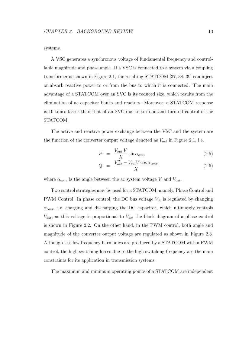
STATCOM Transient Stability (TS) Model
For the case that the output voltage of the STATCOM is balanced and harmonic
free, a TS model has been proposed, which does not include converter switching
phenomena [1, 32]. The STATCOM TS model replaces the detailed model with a
variable voltage source as shown in Figure 2.5, in which the magnitude of capacitor
voltage is determined by a differential equation derived based on the power exchange

CHAPTER 2. BACKGROUND REVIEW 15
refV-
+PI Controller
convα
Phased Locked Loop
(PLL)
for Synchronization
θcosmVV =
+Gate Pulse
Generator
6
o3600 ≤≤ θ
sT
sT
w
w
+1
Supplementary Control
+
+min
max
Magnitude
(rms)
Figure 2.2: STATCOM control block diagram with phase control.
refV
convα
Phased Locked Loop
(PLL)
for Synchronization
Gate Pulse
Generator
6
refdcV
dcV
-
am
max
min
max
min
+
sT
sT
w
w
+1
+
Supplementary Control
s
KK
I
pα
α+
s
KK m
m
Ip ++
-o3600 ≤≤ θ
Magnitude
(rms)
θcosmVV =
Figure 2.3: STATCOM control block diagram with PWM control.

CHAPTER 2. BACKGROUND REVIEW 16
V
maxLImaxcI InductiveCapacitive 0
minV
Figure 2.4: Voltage-Current characteristic of a STATCOM.
between the STATCOM and the network [1, 40]:
dVdc
dt=
3 a k V
CXsin αconv −
Vdc
Rc C(2.7)
where a stands for the transformer ratio, and the resistance Rc represents the
converter losses, which can be significant, depending on the number of switches
and the switching frequency. All the blocks in Figure 2.5 are the same as the
STATCOM detailed model in Figure 2.3, except that the converter and the blocks
related to the switches are replaced by a voltage source kVdc∠θ; the coefficient k
is proportional to the modulation index ma, which for a two-level inverter is ma
2√
2.
It has been shown by means of time-domain simulation results that the TS model
response is reasonably close to that obtained with the detailed model when the
transients are small [1].
CHAPTER 2. BACKGROUND REVIEW 17
Filter
R+j X
convdcVk α∠
+
_dcV
Magnitude
Controller
+
_refdcV
+_
refV
Magnitude
VV θ∠
convα
am (PWM)
P + j Q 1:a
cRC
II θ∠
+
_
Figure 2.5: STATCOM transient stability model and its control [1].
2.3 Power System Stability
From the aforementioned models, a power system model can be represented using
a DAE model, such as :
x = f(x, z, λ, ρ) (2.8)
0 = g(x, z, λ, ρ)
y = h(x, z, λ, ρ)
where x ∈ ℜn is a vector of state variables that represents the state variables of
generators, loads and other system controllers; z ∈ ℜm is a vector of steady state
algebraic variables that result from neglecting fast dynamics in some load phasor
voltage magnitudes and angles; λ ∈ ℜℓ is a set of uncontrollable parameters such as
active and reactive power load variations; ρ ∈ ℜa is a set of controllable parameters
such as tap or AVR set points; and y ∈ ℜl is a vector of output variables such
as power through the lines and generator output power. The nonlinear functions
f : ℜn × ℜm × ℜℓ × ℜa 7→ ℜn, g : ℜn × ℜm × ℜℓ × ℜa 7→ ℜm, and h : ℜn × ℜm ×

CHAPTER 2. BACKGROUND REVIEW 18
ℜℓ ×ℜa 7→ ℜl stand for the differential equations, algebraic constraints and output
variable measurements, respectively.
The DAE model in (2.8) can be linearized about an operating point (xo, zo, λo,
ρo) to obtain the system state matrix A:
A = Dxf |o −Dzf |o Dzg |−1o Dxg |o (2.9)
For slowly varying parameters λ, the power system model (2.8) has been shown
to present local bifurcations, on which most stability indices in the current literature
are based [41].
2.3.1 Voltage Stability
In a power system, voltage stability is directly related to the voltage on the system
buses, and is defined as the power system ability to maintain steady acceptable
voltages at all buses under normal operating conditions and after a contingency
[33]. Thus, if the bus voltage magnitude decreases as the reactive power injection
at the same bus increases, the power system is voltage unstable. This may lead to
voltage collapse, if generators or other reactive power sources do not provide enough
reactive power support. Voltage collapse can be explained within the context of
bifurcation theories applied to DAEs in nonlinear systems, namely, SNB and LIB
[7, 9].
Saddle-node Bifurcations (SNB)
When the system state matrix A has a simple and unique zero eigenvalue with
nonzero left and right eigenvectors, the equilibrium point (xo, zo, λo, ρo) is typically

CHAPTER 2. BACKGROUND REVIEW 19
referred to as SNB point (other transversality conditions must also be met). In
power systems, this bifurcation point is associated with voltage stability problems
due to the local merger and disappearance of equilibria (operating points) as λ
changes.
Limit-induced Bifurcations (LIB)
LIBs occur at an equilibrium point where the eigen-system of A undergoes a discrete
change due to the fact that system states or algebraic variables reach a limit. There
are various types of LIBs, of which a saddle LIB (SLIB) can be associated in power
systems with voltage stability problems due to the local merger and disappearance
of equilibrium points as λ changes.
2.3.2 Angle Stability
Angle stability is defined as the ability of interconnected synchronous machines
to remain in synchronism [33]. In general, the angle instability may happen in
the form of steady increase in rotor angle or undamped rotor oscillations; these
phenomena are due to insufficient synchronizing torque and lack of damping torque,
respectively. This thesis concentrates on the latter. These oscillations are due to
poorly damped or undamped modes that are classified into local modes, inter-
area modes, control modes, and torsional modes. Power system oscillations can be
studied by Hopf bifurcation (HB) theory, which describes the onset of an oscillatory
problem in nonlinear systems.

CHAPTER 2. BACKGROUND REVIEW 20
Hopf Bifurcations (HB)
In this case, two complex conjugate eigenvalues of A cross the imaginary axis as λ
changes. This results in limit cycles that may lead to oscillatory instabilities, as it
has been observed in practice [5, 42].
2.4 Tools
As explained before, power system stability analyses are classified into static and
dynamic studies. In general, voltage stability analysis requires only static data,
such as power flow data and dispatching scenarios, and is investigated by tracing
P-V curves, which are obtained my means of continuation power flow techniques
or optimal power flows. On the other hand, angle stability analyses require both
static and dynamic data (e.g. exciter data), and hence are computationally more
demanding when compared to voltage stability studies. An overview of all the
utilized techniques and tools in this thesis follows.
2.4.1 Continuation Power Flow
For given dispatch scenarios, the continuation power flow [43] technique is used to
obtain P-V curves similar to the one depicted in Figure 2.6, and thus determine the
static loading margin (SLM) of the system (nose point) associated with a voltage
collapse point, which could be the result of an SNB or an LIB. Figure 2.6 also
demonstrates the dynamic loading margin (DLM) of a system, which is associated
with an angle instability happening before the nose point.
All the P-V curves in this work have been obtained with the University of
Waterloo Power Flow (UWPFLOW) program, which is computationally efficient,

CHAPTER 2. BACKGROUND REVIEW 21
0.5
1.0
.).( upV
.
Voltage Instability
.
Angle Instability
SLM
DLM
0LP1maxLP
2maxLPLP
Figure 2.6: A typical PV curve and corresponding SLM and DLM.
as it has been developed in C and C++, and hence appropriate to study large
systems. Furthermore, UWPFLOW provides other insightful information such the
type of bifurcation and the corresponding right and left eigenvectors, plus power
flow solutions and Jacobians.
2.4.2 Small-Disturbance Stability Analysis
As explained before, matrix A and its eigenvalues can provide valuable information
about the system stability for small perturbations that may occur in the system.
This is also referred to as small-disturbance stability analysis or eigenvalue analysis.
In this work, matrix A and its eigenvalues for the test cases have been ob-
tained by means of the linearized transient stability models in the Power System
Toolbox (PST) [36], which is a MATLAB based program. PST, when compared to

CHAPTER 2. BACKGROUND REVIEW 22
other programs, is user-friendly but slow, and hence inappropriate for large systems
(more than 50 buses). Therefore, for large systems, the Small Signal Analysis Tool
(SSAT) is used; as it is able to deal with systems made up of several thousand buses.
It offers powerful features, such as complete eigenvalue analysis; Single-Machine-
Infinite-Bus (SMIB) analysis; eigenvalue analysis within specified frequency and
damping ranges; computation of modes closest to a specified frequency and damp-
ing; computation of modes related to a generator; sensitivity analysis; mode trace;
etc.
2.4.3 Time-Domain Simulation
Time-domain simulation is mainly used for transient stability analysis of power
systems following large perturbations, as it accounts for all the nonlinear effects by
solving the complete set of DAEs by means of step-by-step trapezoidal or predictor-
corrector integration [33]. However, in this thesis, this time-domain response of the
power system is also used to obtain important small-disturbance stability informa-
tion. Time-domain simulations of test cases were carried out by means of both the
PST and the Transient Stability Analysis Tool (TSAT) [44]; however, the simula-
tion of large systems was only feasible with the later. TSAT has two simulation
engines: A conventional time-domain simulation engine that uses full numerical
integration techniques and a fast time-domain simulation engine based on a quasi
steady-state system model. It has several useful features for transient stability anal-
ysis, such as the possibility of running multi-contingency cases or multi-dispatch
scenarios, obtaining a security index based on critical clearing time, etc. A wide
range of dynamic models of power system components is available, and well-known
formats, such as PTI PSS/E, GE PSLF, and BPA can be used as input data.

CHAPTER 2. BACKGROUND REVIEW 23
2.4.4 Identification
System identification is about building mathematical models of complex systems
by using physical insights into the system and the measured input-output data.
It is a useful tool, for a wide range of applications, including obtaining simplified
models for large systems, model validation and controller tuning.
The advantage in studying power systems by means of system identification
techniques is twofold: First, their studies take shorter time, when compared to
analytical techniques that are based on DAE models of the power system, since
the latter usually requires handling equations with several thousand states for a
medium size power system; hence, identification techniques are of interest for on-line
practical system monitoring. Second, these techniques rely on the actual response
of the power system, as opposed to models that are based on approximate system
representation and data.
Since the main objective of this research is to investigate the small-disturbance
stability of the power system, linear parametric models have been used to study
the indices proposed in this thesis. For the first proposed index, the prediction
error method (PEM) and the stochastic subspace identification method are used to
estimate the linear model parameters, and then use the model to extract the modal
content of the time-domain response of the power system. For the second index,
the PEM is used to estimate damping torque coefficients of individual generators,
which in turn provides useful information about the current stability conditions
and margins of the system under study.
The System Identification Toolbox [45] in MATLAB and ad-hoc coding are the
basic tools used to perform these studies.

CHAPTER 2. BACKGROUND REVIEW 24
1G
Figure 2.7: Single-Machine-Infinite-Bus (SMIB).
2.5 Test Systems
A variety of test cases, ranging from a Single-Machine-Infinite-Bus (SMIB) to a real
power system with 14,000 buses, were used to test the feasibility of the proposed
stability indices and system identification techniques. In some cases, several dis-
patch scenarios were considered in order to emulate the operation of a real power
system. The general characteristics of these test cases are briefly reviewed in this
section.
2.5.1 Single-Machine-Infinite-Bus (SMIB)
This is the simplest but the most widely used test case, as it consists of only a
generator, a transmission line and a load as depicted in Figure 2.7. The load
bus is modeled as an infinite bus, which is normally used to replace a stiff large
system with a constant voltage magnitude and angle. This system can be used
to investigate the behavior of a generator or group of generators, labeled as G1 in
Figure 2.7, with respect to the infinite bus.
2.5.2 IEEE 3-bus System
This corresponds to a case where two areas are connected through a long transmis-
sion line (weak connection); hence, power oscillations are observed in the tie-line.

CHAPTER 2. BACKGROUND REVIEW 25
~
1
~
G1 G23 2
Load
Figure 2.8: IEEE 3-bus test system.
A single-line diagram of the test system is shown in Figure 2.8 [8]. The base load
used at Bus 3 is a 900 MW and 300 MVar load, and is modeled as a constant PQ.
Each machine has a simple exciter, and a simple governor is used for the machine
at Bus 1. The generators are modeled in detail by means of subtransient models.
The corresponding static and dynamic data is presented in Appendix A.1.
2.5.3 IEEE 14-bus System
This test system is shown in Figure 2.9, and has 5 generators; two of them are
providing both active and reactive power at Buses 1 and 2, and the generators at
Buses 3, 6 and 8 are basically synchronous condensers [46]. The generators are
modeled by means of subtransient models and equipped with DC exciters (type 1),
and the loads are represented as constant impedances. The base total loading level
of the system is 259 MW and 81.3 MVar. The corresponding static and dynamic
data is presented in Appendix A.2.
2.5.4 Two-area Benchmark System
A single-line diagram of this system is shown in Figure 2.10 [33]. This is similar
to the IEEE 3-bus test system in the sense that two areas are connected through

CHAPTER 2. BACKGROUND REVIEW 26
G
C
G
C
C
1
2
3
4
7 8
9
1011
12
13
14
G
C
GENERATORS
SYNCHRONOUS
THREE WINDING
TRANSFORMER EQUIVALENT
9
4
78
C
6
5
COMPENSATORS
Figure 2.9: IEEE 14-bus test system.

CHAPTER 2. BACKGROUND REVIEW 27
G1
G2
G3
G4
7 1
2
9 3
4
5 6 8 11 10
Area 1 Area 2
Figure 2.10: Two-area benchmark system.
tie-lines, hence resulting in an inter-area mode with a frequency of about 0.7 Hz.
However, the individual machines in each area also contribute to a local mode in
the same area with a frequency of about 1.3 Hz. Therefore, an inter-area rotor
angle mode and two local modes are observed for this test case.
The generators were modeled using subtransient models and their exciters are
simple exciters equipped with PSSs. The corresponding static and dynamic data is
given in Appendix A.3. The total base loading level is 2734 MW and 200 MVar.
2.5.5 Real 14,000-bus System
This system consists of around 2,000 generators, 11,000 lines, 6,000 transformers, 22
areas and 6,500 loads (the details of the system are confidential); the total loading
level of the system is 38.6 GW. Due to the extremely large size of the system, all
the system studies such as power flow, continuation power flow, small-disturbance
stability analysis, and time-domain simulations were carried on PSAT [47], VSAT
[48], SSAT [49], and TSAT [44], respectively.

CHAPTER 2. BACKGROUND REVIEW 28
2.6 Summary
A brief explanation of some of the key power system components used in this
thesis, such as loads and generators, is presented in this chapter. Also discussed
in this chapter is the importance of selecting the right models for different kinds
of analyses. Power system stability concepts and the analysis techniques and tools
used throughout this thesis, such as voltage and angle stability, continuation power
flow and system identification are briefly explained.

Chapter 3
System Identification Techniques
3.1 Introduction
Real-time signals measured in power systems represent the true response of these
systems, as opposed to those obtained through simulation. These signals may be
analyzed by means of signal processing techniques to obtain useful information,
such as stability conditions, about the system. However, these techniques must be
selected properly to ensure that the analysis results are both accurate and depend-
able. In order to capture the dynamic response of a power system, first it must be
excited, a process that is based on either an external test (ringdown test), such as
line/load tripping, or the existing random load switching happening throughout a
day. A “proper” identification technique is then required to analyze the measure-
ments.
This chapter discusses and categorizes the types of signals that can be readily
measured in a power system, and the corresponding techniques used to extract the
modal content of the signals. This modal content, in turn, provides useful informa-
29

CHAPTER 3. SYSTEM IDENTIFICATION TECHNIQUES 30
tion about the system stability conditions. Depending on the kind of excitations
that are present in the system, one can categorize the measured signals as deter-
ministic ringdown data and stochastic ambient data. Thus, each type of data is
explained here thoroughly, as are the corresponding appropriate techniques; the
merits and disadvantages of the techniques are also discussed. A computationally
efficient identification method is then proposed to overcome the shortcomings of
previously used methods.
3.2 Ringdown Data
A power system may be excited by large perturbations (e.g. adding/removing large
loads, generator tripping, severe short circuits), resulting in a transient response
that can be easily observed and distinguished from ambient noise. These transients
usually consist of one or several damped sinusoidal signals. Many techniques can
be deployed to extract the modal content of these transients. Linear techniques are
based mainly on the Prony method [50] and the Matrix Pencil method [51]. The
Prony method is explained below, since it has been widely used in power systems
in order to extract modal content and tune power system controllers such as power
system stabilizers (PSSs) [21, 52, 53, 54].
3.2.1 Prony Method
The Prony method, proposed in 1795 by Gaspard Riche, Baron de Prony, is a viable
technique to model a linear sum of damped exponentials. It was first used to explain
the laws governing the expansion of various gases, and is closely related to the least
square linear prediction algorithms used for AR parameter estimation. However,

CHAPTER 3. SYSTEM IDENTIFICATION TECHNIQUES 31
the Prony method is used to fit a deterministic exponential model to evenly sampled
data, as opposed to the AR and ARMA methods, which are based on a random
model. Several versions of the original Prony method, such as the total least square
Prony method and the singular value decomposition (SVD) Prony method, have
improved its performance.
A measured signal y(t) can be represented in continuous and discrete time,
respectively, as a sum of n damped complex sinusoids:
y(t) =n∑
i=1
Ri eλit =
n/2∑
i=1
Ai eαit cos(βit + φi) (3.1)
y[k] =n∑
i=1
Ri Zki (3.2)
where Ri is an output residue corresponding to the mode λi = αi + jβi; Zi = eλiTs ;
Ts is the sampling time; Ai = 2∣∣Ri
∣∣; and k is integer time.
The original Prony method calculates λi and Ri as follows:
1. Consider that (3.1) is the solution to a difference equation with order n:
y[k] = −a1 y[k − 1] − a2 y[k − 2] − . . . − an y[k − n] (3.3)
This can be written in a matrix form:
Y = D θ (3.4)
where
Y = [yk+n yk+n+1 yk+n+2 . . . yk+N ]TN−n+1 (3.5)
θ = [−a1 − a2 . . . − an]T (3.6)

CHAPTER 3. SYSTEM IDENTIFICATION TECHNIQUES 32
D =
yk+n−1 yk+n−2 . . . yk
yk+n yk+n−1 . . . yk+1
...
yk+N−1 yk+N−2 . . . yk+N−n
(N−n+1)×n
(3.7)
where N is the number of samples. The least square method can be used to
compute θ.
2. The vector θ leads to the eigenvalues Z ,is of the system, which are the roots
of the system characteristic equation:
Zn + a1 Zn−1 + a2 Zn−2 + . . . + an = 0 (3.8)
3. One may write (3.2) in a matrix form similar to (3.4) using the calculated
Zi’s, and solve for the residues Ri’s.
The order of the system n is usually unknown. In [20], the “rule-of-thumb” of an
initial guess for n = N/6 is proposed. Once the roots of the system characteristic
equation are obtained, the poles corresponding to high frequencies, which are known
not to be present in power systems, are discarded. This technique, however, may
lead to results that depend heavily on the user. Furthermore, order underestimation
results in inaccurate results; on the other hand, higher orders lead to accurate
poles estimation as well as extraneous poles, since the model seeks to fit the noise
corrupting the signal.
A better technique for choosing n is proposed in [55] for communication systems.
This method is based on monitoring the singular values of matrix D for n = N/2 .
Although the maximum possible order, which can be chosen for the system, is N/2,
the practical order of a matrix is equal to the number of its largest singular values.
Thus, for σ1 ≥ σ2 ≥ . . . ≥ σn ≥ . . . ≥ σN/2, if σn+1 ≈ σn+2 ≈ ... ≈ σN/2 ≈ 0, then
n < N/2 is the order of the matrix D.

CHAPTER 3. SYSTEM IDENTIFICATION TECHNIQUES 33
When SNR is low, the Prony method is known to behave poorly, and yields
biased and sensitive results since (3.3) no longer holds [56]. Its performance and
problems in the presence of noise have been investigated in [57]. In this paper, the
Prony method is shown to be unable to extract the true poles of the signal if the
SNR is below a certain level; however, this level is higher for signals containing
more modes. For instance, in the case of a single mode comprising the entire
signal, a minimum SNR in the range of 10 to 20 db is required. Furthermore,
it is mentioned that the real part of the mode is more sensitive to noise than its
frequency. Hence, the Prony method is recommended as an appropriate tool to
analyze the measured transient response of power systems with large disturbances,
such as major contingencies or artificially added and removed loads, i.e. ringdown
test.
3.3 Ambient Data
The load switching throughout the day, which is random in nature, are persistently
exciting the power system. Hence, the response of the power system contains
information about the dynamic behavior of the system, and it can be employed
for on-line system stability monitoring. However, these perturbations normally
appear as noise with very small magnitudes on ambient data, and therefore, cannot
be easily distinguished from measurement noise. Due to the randomness of the
perturbations, in order to model the measured signals, a stochastic framework has
to be employed. Well-known linear models such as AR or ARMA have been used
for this purpose; the underlying assumption in this case is that the system input is
noise and so is the output. The input noise is assumed to be white in the frequency
range of interest (0.1 Hz - 2 Hz). The output signal, however, would be a colored

CHAPTER 3. SYSTEM IDENTIFICATION TECHNIQUES 34
noise, since its power spectrum density (PSD) is proportional to the system transfer
function, i.e.
Soutput(f) = |Gs(f)|2 Sinput(f) (3.9)
where Gs(f) is the system transfer function, f is the frequency, and Sinput(f) is the
input signal PSD, which is assumed to be flat in the frequency range of interest.
Thus, output signal in this case can provide insightful information about the system
transfer function. The PSD of a discrete signal such as x[k] is the Fourier transform
of its autocorrelation function (ACF) rxx[k], which is defined as:
rxx[τ ] = E [x∗[k]x[k + τ ]] (3.10)
where τ is the lag time between the two samples, and E denotes the expectation
operator. In this work, it is assumed that the process is wide-sense stationary.
That is, the mean and the ACF do not depend on time, i.e. the ACF in (3.10) only
depends on the lag time τ .
3.3.1 ARMA Model
The power system linearized model may be represented as a time series or a rational
transfer function. That is, the output y[k] and input noise e[k], which represents
the load switching throughout the day, are related in a linear difference form,
y[k] = −p
∑
i=1
ai y[k − i] +d∑
i=0
bi e[k − i] (3.11)
where ai’s and bi’s represent the coefficients related to the AR and MA terms,
respectively, and p and d denote the order of the AR and MA terms, respectively.
This is known as an ARMA(p,d) model. It is important to mention that the input
noise or process noise is different from the measurement or observation noise.
CHAPTER 3. SYSTEM IDENTIFICATION TECHNIQUES 35
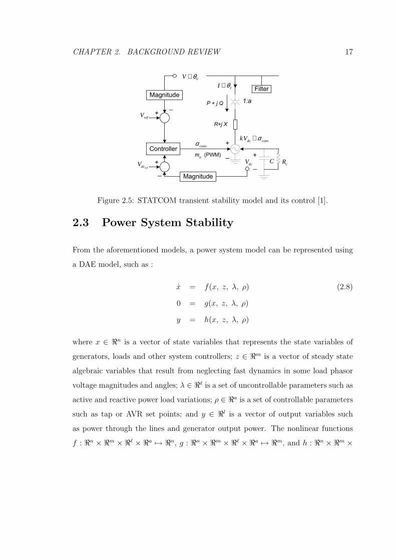
The system transfer function Gs(q) between the output and the input is defined
as:
Gs(q) =B(q)
A(q)(3.12)
A(q) =
p∑
i=0
ai q−i , a0 = 1
B(q) =d∑
i=0
bi q−i
where q is the shifting operator defined by q−1y[k] = y[k− 1]. The roots of polyno-
mial A(q) yield the poles of the system. Thus, from (3.9), the relationship between
the input and the output PSDs is,
Sy(f) = σ2
∣∣∣∣
B(f)
A(f)
∣∣∣∣
2
(3.13)
e[k] is assumed to be white noise with variance σ2.
The ARMA(p,d) is a strictly autoregressive model AR(p) if all bk except b0
vanish, and a strictly moving average model MA(d) if all ak except a0 are zero.
According to the Wold decomposition theorem and the Kolmogorov theorem
[56], any ARMA or AR process can be represented by a unique MA process of
infinite order and vice versa. This is important since, if one fails to choose a correct
model structure and a right order for a system, it would still be possible to obtain
a reasonable approximation by choosing an order higher than the true order.
3.3.2 Parameter Estimation
There are different approaches to estimating the parameters of any structure such as
an ARMA model and a state-space model associated with the power system. They

CHAPTER 3. SYSTEM IDENTIFICATION TECHNIQUES 36
mainly fall into the three following categories: Prediction error methods (PEM),
correlation methods and subspace methods; each one providing potential gains as
well as potential pitfalls. Each method is described briefly below [58, 59]:
• Prediction Error Methods: These methods are basically based on performing
an optimization routine to obtain the unknown parameters θ. For instance,
for the ARMA(p,d) model described in (3.11), θ = [a1 ... ap b1 ... bd]T may be
computed by minimizing an objective function such as
Min V (θ) =1
N
N∑
k=1
1
2ǫ2[k] (3.14)
s.t. ǫ[k] = y[k] − y[k]
where ǫ[k] is the prediction error and y[k] is the one-step-ahead prediction of
y[k], and can be mathematically expressed as
y[k] =
[
1 −(
B(q)
A(q)
)−1]
y[k] (3.15)
This requires an iterative search for θ that yields the minimum of loss function
V (θ). The optimization is a nonlinear optimization, and thus may lead to local
minima as well as high computational burden. In this work, however, only the
coefficients of polynomial A(q) are of interest, since it is aimed at extracting
the modal content of the signal, which are the roots of A(q). Hence, one may
consider applying other techniques such as the Yule-Walker (YW) method
that only estimates the parameters of A(q), thus employing more simplified
and robust numerical techniques. It is also possible to model y[k] in (3.11)
with a high-order AR rather than using an ARMA as a result of Kolmogorov
theorem. This leads to an objective function that can be solved by means of
well-known least square method; thus, the least square used for an AR model

CHAPTER 3. SYSTEM IDENTIFICATION TECHNIQUES 37
would be identical to that of the Prony method. A high-order AR, however,
leads to extraneous poles close to the system poles, which could be difficult
to distinguish between the true and extraneous modes. Furthermore, an AR
model may result in biased estimates if residuals are not white. As previously
mentioned for the Prony method, when the SNR is low, the model structure
is an ARMA rather than a pure AR.
• Correlation Methods: The fundamental idea behind correlation methods is
that, for a good model, the prediction error at time k should be independent
of past data up to time k − 1, i.e. if the errors are correlated with past data,
then there was more information available in past data about y[k] than picked
by y[k]. Normally, similar to the PEM, correlation methods require an iter-
ative search technique to solve a nonlinear equation. However, Instrumental
variable (IV) methods as an application of the correlation methods result in
a linear regression. A special case of IV methods are shown to be the YW
method [60] (a set of linear equations that can be solved by means of fast and
efficient algorithms such as Levinson’s). More details about the fundamentals
of the original YW method and, different versions of YW such as modified YW
(MYW) and least square modified YW (LSMYW) are presented in Section
3.3.3.
• Subspace Methods: Subspace methods have become popular because of their
numerical simplicity, robustness of the techniques that are used in the algo-
rithms, and their state-space form which is convenient for control purposes
[61]. However, subspace methods are suboptimal, as they are not based on the
minimization of a criterion. Some of the main advantages of these methods
over previously mentioned identification methods are:

CHAPTER 3. SYSTEM IDENTIFICATION TECHNIQUES 38
1. Model order selection: For PEM, different criteria have been proposed
in order to select the best order of the model, such as Akaike Infor-
mation Criterion (AIC) and Final Prediction Error (FPE) [58]. These
techniques are defined based on prediction error variance. For instance,
to choose the orders p and d of an ARMA(p,d) model, first a range is se-
lected for p and d, then, for each (p,d) pair, the parameters of the model
are estimated; the pair obtaining the lowest value of AIC or FPE crite-
rion is selected as the best estimate of the model order. This approach
results in high computational costs since, in order to obtain the predic-
tion error variance, all the possible models in the selected range have
to be first estimated. On the other hand, in subspace methods, there is
the possibility to estimate the model order without having to estimate
the parameters of a variety of different models. Order estimation in this
case is one step of the algorithm, and only requires a SVD.
2. Handling large data: When the amounts of data are large, order selection
with PEM based techniques is just not feasible [62]. This is the case
of the application being considered in this thesis, which requires long
“blocks” of data in order to truly estimate the power system mode(s).
3. On-line application: If for any reason, the system dynamics change, the
model needs to be updated. The subspace methods are a better choice
in this case, due to the superiority of subspace over other methods from
a computational point of view [62].
The state-space matrices are identified in this case by using measured outputs
and robust numerical techniques such as QR-factorization, least square and
SVD without the need to calculate correlations, i.e. it is data driven instead of
covariance driven. Therefore, these types of techniques are computationally

CHAPTER 3. SYSTEM IDENTIFICATION TECHNIQUES 39
more efficient.
3.3.3 AR Parameter Estimation
Several approaches can be utilized to estimate the parameters of the coefficients of
the polynomial A(q) in an AR or ARMA model. They all result in a set of linear
equations that relates the parameters with the help of the ACF. The basic YW
equation is explained, and the variations of YW to overcome its shortcomings are
then presented.
Yule - Walker (YW)
For a strictly AR process, equations (3.11) is rewritten as:
y[k] = −p
∑
i=1
ai y[k − i] + b0 e[k] (3.16)
Multiplying both sides of (3.16) by y[k − j] and taking the expectation yields:
ryy[j] =
−p∑
i=1
ai ryy[j − i] for j ≥ 1
−p∑
i=1
ai ryy[−i] + b0 σ2 for j = 0
(3.17)
This equation is known as YW equation, and defines a relationship between the
ACF and parameters of an AR(p) process. By solving the following set of linear
equations, one can determine the parameters of an AR(p):
ryy[0] ryy[−1] · · · ryy[−(p − 1)]
ryy[1] ryy[0] · · · ryy[−(p − 2)]...
.... . .
...
ryy[p − 1] ryy[p − 2] · · · ryy[0]
︸ ︷︷ ︸
Ryy
a1
a2
...
ap
= −
ryy[1]
ryy[2]...
ryy[p]
(3.18)

CHAPTER 3. SYSTEM IDENTIFICATION TECHNIQUES 40
The autocorrelation matrix Ryy is hermitant (RHyy = Ryy), and Toeplitz since the
diagonal elements (top-left to lower-right) are the same. The model in this case
yields stable poles [56]. Equation (3.18) may be solved by means of an efficient algo-
rithm such as Levinson’s, and it depends on the ACF. A reasonable approximation
is to calculate the elements of Ryy from the limited available data.
Modified Yule - Walker (MYW)
A similar procedure previously used to derive the YW equation can be applied to
an ARMA(p,d) model, leading to the following set of linear equations:
ryy[d] ryy[d − 1] · · · ryy[d − p + 1]
ryy[d + 1] ryy[d] · · · ryy[d − p + 2]...
.... . .
...
ryy[d + p − 1] ryy[d + p − 2] · · · ryy[d]
︸ ︷︷ ︸
R′
yy
a1
a2
...
ap
= −
ryy[d + 1]
ryy[d + 2]...
ryy[d + p]
(3.19)
The matrix R′
yy is Toeplitz, although not hermitant. Hence, the stability of the
poles of A(q) is not guaranteed [56].
Least Square Modified Yule - Walker (LSMYW)
Equation (3.19) could also be rewritten as:
ryy[k] = −p
∑
i=1
ai ryy[k − i] for k ≥ q + 1 (3.20)

CHAPTER 3. SYSTEM IDENTIFICATION TECHNIQUES 41
Since there is information in the ACF with higher order lags, it is also possible to
calculate the ai’s by incorporating these ACFs. Thus:
ryy[d] ryy[d − 1] · · · ryy[d − p + 1]
ryy[d + 1] ryy[d] · · · ryy[d − p + 2]...
.... . .
...
ryy[M − 1] ryy[M − 2] · · · ryy[M − p]
︸ ︷︷ ︸
R′′
yy
a1
a2
...
ap
= −
ryy[d + 1]
ryy[d + 2]...
ryy[M ]
(3.21)
In this case, M − d ≥ p and R′′ ∈ ℜ(M−d)×p is a nonsquare matrix, as opposed to
R′ ∈ ℜp×p; hence, the least square method has to be employed to calculate the ai’s.
It is stated in [56] that for large data records, the estimates obtained by solving
LSMYW equations are asymptotically unbiased, and that its variance decreases as
the number of equations (M − d) increases, as long as N ≫ M − d. In general,
LSMYW offers better performance compared to MYW if the number of equations
is not too large. As reported in [56], LSMYW yields the most accurate estimates
when the poles are near the unit circle. This is usually the case in a power system
with poorly damped oscillations, as the corresponding poorly damped modes are
the ones with damping ratios less than 3%, i.e. the power system controllers (e.g.
PSS) are well-tuned if the modes attain a minimum damping ratio of 3%.
Comparison
The previously explained YW method and its variations are compared here with
the PEM based on estimating the parameters of an AR(10) or ARMA(10,5) for
detection of an electromechanical mode. A two-minute recorded power signal PG2
in the two-area benchmark system is used as the system output y[k] (for more details
regarding the test system, please refer to Chapter 2). The input is simulated as

CHAPTER 3. SYSTEM IDENTIFICATION TECHNIQUES 42
random load switching, and 20 simulations with independent realizations of the
noise yield the results depicted in Figure 3.1. The order of the system is selected
to be 10 for the YW method. On the other hand, an ARMA(10,5) is assumed for
both MYW and LSMYW methods, but the number of linear equations in (3.19)
and (3.21) are different, i.e. 10 and 15, respectively. Observe that the YW method
does the poorest job in estimating the electromechanical mode with a high variance,
while providing stable poles, as mentioned in Section 3.3.3. However, some of poles
estimated with the MYW and the LSMYW methods are unstable. The LSMYW
performance is better than both the YW and the MYW methods, and comparable
to the PEM results in terms of accuracy and variance. On the other hand, the long
computational times needed by the optimization routine required in the PEM, and
the associated numerical problems are drawbacks of using the PEM.
3.3.4 Stochastic Subspace Identification
Consider the discrete stochastic state-space model:
∆x[k + 1] = Ad ∆x[k] + w[k], Ad = eA Ts (3.22)
∆y[k] = C ∆x[k] + v[k]
where ∆x[k + 1] is the discrete time state vector; w[k] and v[k] are zero mean
noise E[w[k]] = E[v[k]] = 0 representing the process noise and the measure-
ment noise, respectively, and are independent from ∆x[k], i.e. E[∆x[k].wT [k]] = 0,
E[∆x[k].vT [k]] = 0; and A and Ad denote the continuous and discrete time state
matrices, respectively. The output measurements are put into a block Hankel ma-

CHAPTER 3. SYSTEM IDENTIFICATION TECHNIQUES 43
−0.8 −0.7 −0.6 −0.5 −0.4 −0.3 −0.2 −0.1 0 0.14.65
4.7
4.75
4.8
4.85
4.9
4.95
5
5.05
5.1
5.15
Real (sec−1)
Ima
gin
ary
(ra
d/s
ec)
AR(10) with YWARMA(10,5) with MYWARMA(10,5) with LSYWARMA(10,5) with PEM
True mode
Figure 3.1: The performance of YW, MYW, LSMYW, and PEM in electromechan-
ical mode estimation from ambient data.
CHAPTER 3. SYSTEM IDENTIFICATION TECHNIQUES 44
trix, and divided into a past and future parts as follows:
Y0|2i−1 =
∆y[0] ∆y[1] . . . ∆y[j − 1]
∆y[1] ∆y[2] . . . ∆y[j]
. . . . . . . . . . . .
∆y[i − 1] ∆y[i] . . . ∆y[i + j − 2]
∆y[i] ∆y[i + 1] . . . ∆y[i + j − 1]
∆y[i + 1] ∆y[i + 2] . . . ∆y[i + j]
. . . . . . . . . . . .
∆y[2i − 1] ∆y[2i] . . . ∆y[2i + j − 2]
=
(Y0|i−1
Yi|2i−1
)
=Yp
Yf
(3.23)
where i is typically equal to 2M/l [61], with M representing the “expected” maximal
order of the system, and j is the number of samples of each measured output signal.
The subscripts of Y0|2i−1, Y0|i−1 and Yi|2i−1 are the first and last element in the first
column of the block Hankel matrix. Matrices Y +p and Y −
f are defined by shifting
the border between past and future data one row down in (3.23), i.e. Y +p = Y0|i,
and Y −f = Yi+1|2i−1.
There are different algorithms to calculate the system matrices Ad and C. The
canonical variate algorithm (CVA) is used here as explained below.
Canonical Variate Algorithm [61]
Once the block Hankel matrix and its submatrices are formed, the following steps
are taken:

CHAPTER 3. SYSTEM IDENTIFICATION TECHNIQUES 45
1. Calculate the projection matrices Oi and Oi−1:
Oi = Yf/Yp (3.24)
Oi−1 = Y −f /Y +
p (3.25)
where Yf/Yp denotes a shorthand for the projection of the row space of the
future matrix Yf on the row space of past matrix Yp, i.e. YfYTp (YpY
Tp )†Yp
where the symbol † denotes the pseudo inverse of the matrix. Robust QR-
factorization methods may be used to calculate the projection matrices.
2. Calculate the SVD of the weighted projection:
W1OiW2 = USV T (3.26)
= (U1 U2)
S1 0
0 0
V T
1
V T2
where weighting matrices W1 =(
1jYfY
Tf
)− 1
2
, and W2 = Ij (identity matrix
j × j); and U and V are unitary matrices resulting from the SVD process.
The order of the system n is determined by inspecting the singular values in
S, i.e. determine the n×n submatrix S1, which are the cosine of the principal
angles between the row space of past outputs Yp and future outputs Yf . In
practice, however, due to noise and rounding errors, the structure of S is not
as shown in (3.26), i.e. the zero diagonal matrix is not really zero. In this
case, a “large” reduction in the singular values of S are used to define S1 (the
system order n), as discussed in detail for the test systems in Chapter 4.
3. Determine the extended observability matrices Γi and Γi−1 as follows:
Γi = W−11 U1S
1/21 (3.27)
Γi−1 = Γi (3.28)

CHAPTER 3. SYSTEM IDENTIFICATION TECHNIQUES 46
where Γi is obtained by removing the last l rows of Γi with l being the number
of output signals.
4. Find the Kalman filter state sequences Xi and Xi+1 as follows:
Xi = Γ†iOi (3.29)
Xi+1 = Γ†i−1Oi−1 (3.30)
5. Then, Ad and C are determined from:
Ad
C
=
Xi+1
Yi|i
X†i (3.31)
Once Ad is calculated, the eigenvalues Zi = ZRi+ jZIi
of matrix Ad can be
transformed onto the s-plane si = λRi+ jλIj
using a bilinear transformation,
i.e. si = 2Ts
(Zi − 1)/(Zi + 1).
3.3.5 Computational Issues
One of the assumptions in stochastic subspace identification is that the w[k] and
v[k] are independent of ∆x[k], i.e. E[∆x[k].wT [k]] = 0, E[∆x[k].vT [k]] = 0. It
is typically assumed that the data blocks are long enough and ergodic, i.e. the
underlying system model is not changing, so that the expectation operator E can
be replaced with the average over one experiment run for infinite time. This is why
subspace methods work well for long data blocks even in the presence of noise [61].
The asymptotic properties of the proposed subspace method are also discussed in
[63], where it is shown that for a white noise input, the CVA and the PEM are
asymptotically equivalent.
The effect of using different sizes of data blocks on the accuracy of the method
was investigated for the 2-area benchmark system, and the asymptotic behavior

CHAPTER 3. SYSTEM IDENTIFICATION TECHNIQUES 47
Table 3.1: CPU time in seconds for different methods and system orders
Method MATLAB function n=13 n=16 n=19 n=22
Subspace n4sid(n) 0.63 0.83 1.00 1.16
ARMA armax(n,n) 6.99 9.96 14.08 19.44
State-space pem(n) 11.17 13.99 24.67 36.20
of the proposed subspace method was compared to an ARMA model and a state-
space model whose parameters were estimated using the PEM. For this purpose,
the following built in functions of MATLAB were used: function n4sid() for the
subspace method; armax() for the ARMA model; and pem() for the state-space
model. The data was generated for an inter-area mode −0.1228±j4.7824 (damping
2.57% and frequency 0.7611 Hz). The standard deviation of the estimated real part
and frequency of the mode for different size of data blocks are depicted in Figure
3.2 and Figure 3.3, respectively; these were obtained based on a Monte-Carlo type
of simulation with 30 independent cases. Notice that for short data blocks, the
ARMA and state-space models yield better performance. On the other hand, for
long data blocks, as explained before, the proposed subspace method and ARMA
and state-space models behave similarly.
From the computational burden point of view, the previously mentioned MAT-
LAB built in functions were used to estimate the parameters of the corresponding
models for the same 4-minute block data. Table 3.1 shows the CPU times obtained
for each function as the system order n changes; observe that the subspace method
is significantly faster than the others.

CHAPTER 3. SYSTEM IDENTIFICATION TECHNIQUES 48
1 1.5 2 2.5 3 3.5 40.02
0.03
0.04
0.05
0.06
0.07
0.08
0.09
0.1
0.11
Block size (minutes)
Sta
nd
ard
de
via
tion
of
α (
sec
−1)
Subspace (n=20)ARMA (20,20)State−space (n=20)
Figure 3.2: Standard deviation of the estimated real part α of the inter-area mode
−0.1228 ± j4.7824 for the 2-area benchmark system.

CHAPTER 3. SYSTEM IDENTIFICATION TECHNIQUES 49
1 1.5 2 2.5 3 3.5 40
0.02
0.04
0.06
0.08
0.1
0.12
0.14
0.16
0.18
Block size (minutes)
Sta
nd
ard
de
via
tion
of fr
eq
ue
cy (
Hz)
Subspace (n=20)ARMA (20,20)State−space (n=20)
Figure 3.3: Standard deviation of the estimated frequency of the inter-area mode
−0.1228 ± j4.7824 for the 2-area benchmark system.

CHAPTER 3. SYSTEM IDENTIFICATION TECHNIQUES 50
3.4 Summary
Different types of signals that can be readily measured in a power system are
described as well as corresponding techniques to extract the modal content of the
signals. This modal content, in turn, provides useful information about the system
stability condition. Depending on the kind of excitations that are present in the
system, appropriate techniques are recommended for both deterministic ringdown
and stochastic ambient data, and the merits and pitfalls of each technique are
discussed. Namely, the Prony method is suitable for the transient response with
high SNR, while the LSMYW and the PEM are shown as proper techniques to
analyze ambient noise.
The stochastic subspace identification method is proposed to capture the critical
modes of a power system from ambient data; it uses robust numerical techniques,
and is data driven instead of covariance driven, and hence is faster. The results
demonstrate the accuracy and efficiency of the proposed method; therefore, it can
be used as an on-line monitoring tool in power system surveillance and electrome-
chanical mode detection. The asymptotic behavior of the proposed method was
also investigated, and compared with the class of estimation methods known as
PEM. It was shown that the methods are asymptotically equivalent; however, the
proposed method is much easier to implement, and is computationally efficient.
Chapter 4
System Identification Stability
Index
4.1 Introduction
The identification of stability limits associated with angle stability is of great in-
terest to Independent System Operators (ISO). The availability of proper on-line
monitoring tools can assist operators to determine the available security margins
of the system, thus allowing them to take proper actions close to real time in the
case of system contingencies.
In this chapter, a general overview is given regarding a previously proposed
oscillatory stability index, which is calculated off-line and is used to predict oscilla-
tory phenomena. A stability index to determine and predict the closest instability
point in a power system with regards to the load change is then proposed and
studied. This index is defined based on the critical eigenvalues of the system, i.e.
the eigenvalues that eventually cross the imaginary axis, thus leading the system to
51

CHAPTER 4. SYSTEM IDENTIFICATION STABILITY INDEX 52
instability. Several test systems, including a real 14,000-bus system, are employed
to test the effectiveness of the proposed index using both their transient response
and ambient noise by means of the Prony method and the stochastic subspace
identification method, respectively.
4.2 Proposed Oscillatory Stability Index
The index, referred in [13] as to Hopf bifurcation index (HBI), predicts the distance
to the closest SNB or HB stability point, given a known load change direction. It
is based on the system state matrix A and the “critical” eigenvalues µc = αc ± jβc,
i.e. the eigenvalues that eventually cross the imaginary axis at an SNB or HB point
as λ changes. Thus, the HBI is defined as
HBI(A, βc) = svmin(Am) (4.1)
where svmin is the minimum singular value of the modified state matrix Am, which
is defined as
Am =
A +βcIn
−βcIn A
2n
(4.2)
At an SNB or HB point, svmin becomes zero. In [13], the authors also compare the
HBI to an eigenvalue index (EVI) which is defined as the real part of the critical
eigenvalue. It is worth mentioning that almost in all test cases both HBI and EVI
present a fairly linear behavior.
Computing the HBI in (4.1) requires making assumptions about the model, so
that the matrix A can be explicitly determined. However, if the “output” deviations

CHAPTER 4. SYSTEM IDENTIFICATION STABILITY INDEX 53
∆y(t) ∈ ℜl of (2.8), i.e.
∆x(t) = A ∆x(t) (4.3)
∆y(t) = C ∆x(t)
is measured, the modal content in the output signal ∆y(t) is the same as the modal
content in matrix A if the system modes are excited; hence, these modes can be
calculated using system identification techniques. If the eigenvalues µi(A) = αi+jβi
of the system can be identified, one may define a new diagonal state matrix Λ =
diagµ1, µ2, . . . , µn, which can be used to define the following new modified state
matrix:
Λm =
Λ +βcIn
−βcIn Λ
2n
(4.4)
In this case, using basic singular value decomposition concepts as shown in Ap-
pendix B, the svmin for Λm can be calculated using:
svmin(Λm) = mini=1,n
√
α2i + (βc − βi)2
(4.5)
If the closest eigenvalue to the imaginary axis is the critical one, then
svmin(Λm) = |αc| (4.6)
Since multiple eigenvalues can be readily determined using system identification
tools applied to measured signals such as generator speed or power, and assuming
that the critical eigenvalue can be monitored, a System Identification Stability
Index (SISI) is hence defined here:
SISI = |αc| (4.7)
Observe that this index does not require assumptions regarding the system modeling
as the HBI would require. Furthermore, based on the observations in [13] regarding
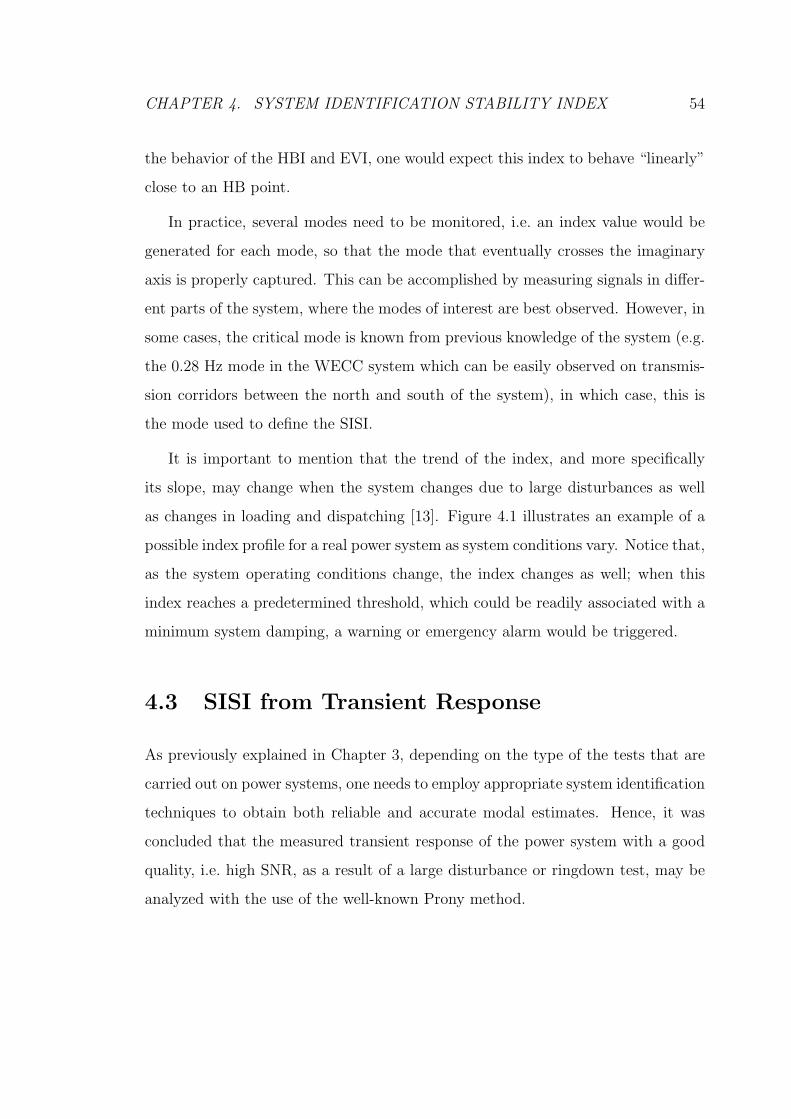
CHAPTER 4. SYSTEM IDENTIFICATION STABILITY INDEX 54
the behavior of the HBI and EVI, one would expect this index to behave “linearly”
close to an HB point.
In practice, several modes need to be monitored, i.e. an index value would be
generated for each mode, so that the mode that eventually crosses the imaginary
axis is properly captured. This can be accomplished by measuring signals in differ-
ent parts of the system, where the modes of interest are best observed. However, in
some cases, the critical mode is known from previous knowledge of the system (e.g.
the 0.28 Hz mode in the WECC system which can be easily observed on transmis-
sion corridors between the north and south of the system), in which case, this is
the mode used to define the SISI.
It is important to mention that the trend of the index, and more specifically
its slope, may change when the system changes due to large disturbances as well
as changes in loading and dispatching [13]. Figure 4.1 illustrates an example of a
possible index profile for a real power system as system conditions vary. Notice that,
as the system operating conditions change, the index changes as well; when this
index reaches a predetermined threshold, which could be readily associated with a
minimum system damping, a warning or emergency alarm would be triggered.
4.3 SISI from Transient Response
As previously explained in Chapter 3, depending on the type of the tests that are
carried out on power systems, one needs to employ appropriate system identification
techniques to obtain both reliable and accurate modal estimates. Hence, it was
concluded that the measured transient response of the power system with a good
quality, i.e. high SNR, as a result of a large disturbance or ringdown test, may be
analyzed with the use of the well-known Prony method.
CHAPTER 4. SYSTEM IDENTIFICATION STABILITY INDEX 55
(c)
Warning
Emergencyng
(d)
(a), (b), (c), (d): Different load and dispatch scenarios (a), (b), (c): Load increases (d): Load decreases
SISI
Time
(a)
(b)
Line outage
Generator tripping
Remedial action (e.g. load shedding)
Figure 4.1: SISI profile for a real power system with varying operating conditions.
The response of the system to a large disturbance, such as a line outage or a three
phase fault, is recorded such that it contains at least three periods of oscillations.
Then, the measurement noise is removed with a Chebyshev low pass filter with a
cut off frequency of 2 Hz, then re-sampling the signal at 10 Hz; the mean and low
frequency trends of the measured signal have to be removed as well. The Prony
method is then applied to the preprocessed signal to obtain the modal contents
of the signal and thus the SISI. The behavior of the index, as the system loading
changes, is depicted below for each test system, illustrating the application of the
SISI to the prediction of the stability margin.
4.3.1 IEEE 3-bus System
The IEEE 3-bus system of Figure 2.8 is used here to test the application of the
proposed index. The P-V curves for the base system and for a line 2-3 outage

CHAPTER 4. SYSTEM IDENTIFICATION STABILITY INDEX 56
are given in Figure 4.2; observe that these cases present HBs at certain loading
conditions before the maximum SLM (nose point). The rotor speed of generator
G1 for a line 2-3 outage is shown in Figure 4.3 for two loading conditions; notice
that at higher loading, the contingency results in unstable oscillations associated
with the HB depicted in Figure 4.2. For a SNR of 30 db, the 8 largest singu-
lar values of the matrix D in (3.7) are 0.26568, 0.24935, 0.0089838, 0.0037355,
0.0000252, 0.0000228, 0.0000067, 0.0000006; hence, the practical order of the sys-
tem is n = 2, as there is a large drop from the second to the third singular value.
Nevertheless, higher orders are examined as well. The characteristic equation can
then be formulated, and the modal content of the signal is obtained using (3.8).
The small-disturbance stability program of the PST program [36] was also used
to obtain the critical eigenvalues from a linearized model of the power system, and
obtain the corresponding EVI of DAE Model. With the variation of the load at
Bus 3, the eigenvalues of the base system and the system under a line 2-3 outage
were computed using PST and the Prony method; the eigenvalue profiles obtained
with PST with respect to load changes in the base system are illustrated in Figure
4.4. For each system, the stability indices (from the linearized DAE model and the
mean value of 30 simulations) are depicted in Figures 4.5 and 4.6. Observe that all
indices predict an HB at about 1500 MW for the base system and 1130 MW for a
line 2-3 outage, with both EVI and SISI indices presenting a rather linear profile.
The results for the Prony method when the SNR is 10 db are shown in Figure
4.7, demonstrating poor results compared with the case when SNR is 30 db, as
expected and explained in Section 3.2.1.
Increasing the model order results in more accurate estimates of the critical
modes, as shown in Figures 4.5, 4.6 and 4.7. However, the order cannot be in-
creased without considering the following: First, the appearance of extraneous

CHAPTER 4. SYSTEM IDENTIFICATION STABILITY INDEX 57
1000 1200 1400 1600 1800 2000 22000.4
0.5
0.6
0.7
0.8
0.9
1
1.1
Total Load (Mw)
V3 (
p.u
.)
Base caseLine 2−3 outage
* * HB
HB
Figure 4.2: P-V curves at Bus 3 for the IEEE 3-bus system, for the base case and
for a line 2-3 outage.

CHAPTER 4. SYSTEM IDENTIFICATION STABILITY INDEX 58
0 2 4 6 8 10 12
0.996
0.997
0.998
0.999
1
1.001
1.002
1.003
1.004
time (sec)
ωG
1
Total load = 900 MwTotal load = 1135 Mw
Figure 4.3: Generator G1 speed following a line 2-3 outage in the IEEE 3-bus
system.

CHAPTER 4. SYSTEM IDENTIFICATION STABILITY INDEX 59
−8 −7 −6 −5 −4 −3 −2 −1 0−20
−15
−10
−5
0
5
10
15
20
Real
Ima
gin
ary
Ho
pf B
ifurc
atio
n
λ
λ
λ
λ λ
Figure 4.4: Eigenvalue profiles with respect to load changes in the IEEE 3-bus
system.
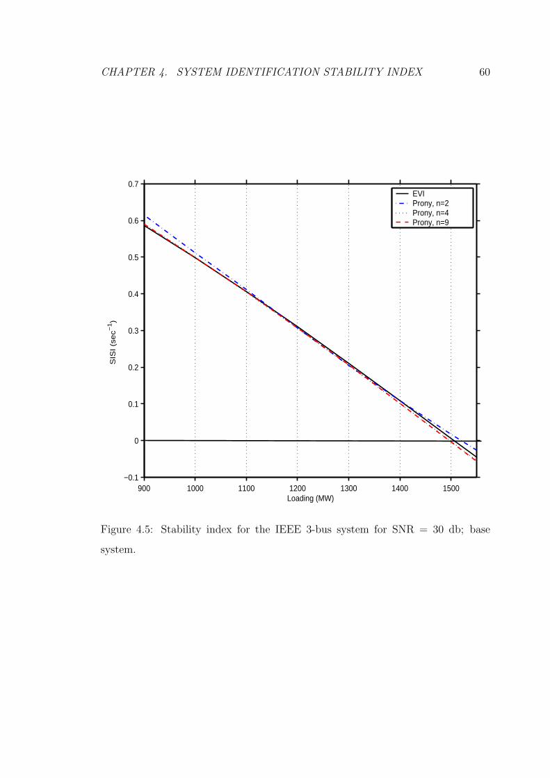
CHAPTER 4. SYSTEM IDENTIFICATION STABILITY INDEX 60
900 1000 1100 1200 1300 1400 1500−0.1
0
0.1
0.2
0.3
0.4
0.5
0.6
0.7
SIS
I (s
ec−
1)
Loading (MW)
EVIProny, n=2Prony, n=4Prony, n=9
Figure 4.5: Stability index for the IEEE 3-bus system for SNR = 30 db; base
system.

CHAPTER 4. SYSTEM IDENTIFICATION STABILITY INDEX 61
900 950 1000 1050 1100 1150−0.05
0
0.05
0.1
0.15
0.2
0.25
0.3
0.35
0.4
Loading (MW)
SIS
I (s
ec−
1)
EVIProny; n = 2Prony; n = 4Prony; n = 9
Figure 4.6: Stability index for the IEEE 3-bus system for SNR = 30 db; line 2-3
outage.

CHAPTER 4. SYSTEM IDENTIFICATION STABILITY INDEX 62
900 1000 1100 1200 1300 1400 1500−0.1
0
0.1
0.2
0.3
0.4
0.5
0.6
0.7
Loading (MW)
SIS
I (s
ec−
1)
EVIProny; n = 2Prony; n = 4Prony; n = 9
Figure 4.7: Stability index for the IEEE 3-bus system for SNR = 10 db; base
system.

CHAPTER 4. SYSTEM IDENTIFICATION STABILITY INDEX 63
modes, which makes it difficult to distinguish between the true modes and spurious
ones. Second, the variance of mode/pole estimates, which is directly related to the
variance of the SISI.
One should make a distinction between the variance of the parameters θ, i.e. co-
efficients of the characteristic equation or coefficients of an AR(p), and the variance
of mode/pole estimates that are the roots of the characteristic equation. There is a
nonlinear relationship between them, and the theoretical background on the former
is well understood and developed. Thus, the variance of the parameters θ is known
to increase asymptotically, as the order increases [58]. Figure 4.8 illustrates this
behavior; observe that when the order of the system increases from 2 to 4 and then
9, there is a significant increase in the variance of the parameters estimates. On
the other hand, no clear conclusion can be reached regarding the variance of pole
estimates when the order changes. This can be clearly observed in Figure 4.9, which
shows the standard deviation of pole estimates, depicted with use of the standard
deviation of both the SISI and the frequency.
4.3.2 IEEE 14-bus System
The IEEE 14-bus benchmark system shown in Figure 2.9 is used as a more realistic
test system. There is an HB point for both the base system and for a line 2-4
outage before the “nose” point, as shown in the corresponding P-V curves depicted
in Figure 4.10. The base system yields the critical eigenvalues µc = −0.21637 ±j8.8298 (1.4 Hz frequency and 2.45% damping ratio) at a 259 MW load; this is the
eigenvalue that eventually crosses the imaginary axis at the HB point, as shown in
the eigenvalue profiles depicted in Figure 4.11.
The stability indices for the base system and for a line 2-4 outage are depicted

CHAPTER 4. SYSTEM IDENTIFICATION STABILITY INDEX 64
a_1a_2
a_3a_4
a_5a_6
a_7a_8
a_9
0
0.1
0.2
0.3
0.4
0.5
Parameters
Stn
da
rd d
evi
atio
n o
f θ
Prony; n = 2Prony; n = 4Prony; n = 9
Figure 4.8: Standard deviation of parameter estimates for the IEEE 3-bus system;
ai’s are the characteristic equation coefficients.

CHAPTER 4. SYSTEM IDENTIFICATION STABILITY INDEX 65
900 1000 1100 1200 1300 1400 15000.02
0.04
0.06
0.08
0.1
Loading(MW)
Sta
nd
ard
de
via
tion
of S
ISI (s
ec−
1)
Prony; n = 2Prony; n = 4Prony; n = 9
900 1000 1100 1200 1300 1400 15000
0.005
0.01
0.015
0.02
Loading(MW)
Sta
nd
ard
de
via
tion
of fr
eq
ue
ncy
(H
z)
Figure 4.9: Standard deviation of the SISI and the critical mode’s frequency for
the IEEE 3-bus system.

CHAPTER 4. SYSTEM IDENTIFICATION STABILITY INDEX 66
in Figures 4.12 and 4.13, respectively. Observe that SISIs in this case are not as
close to the EVI values as in case of the IEEE 3-bus system. This can be explained
by looking at the time-domain response of the system as depicted in Figure 4.14.
Note that the 1.4 Hz signal (fast) does not oscillate about the pre-contingency
operating condition as opposed to Figure 4.3; hence, the identified indices, when
compared with the IEEE 3-bus system results, deviate significantly from the EVI
model values. This behavior is due to the fact that the type of load models used
in the IEEE 3-bus and 14-bus systems are different; for the IEEE 3-bus system,
the constant PQ load model makes the time-domain response oscillate about the
pre-contingency conditions.
4.3.3 Real System (14,000 buses)
In order to investigate the shape of the proposed index for a real power system, a
14,000-bus system is studied. To move this system closer to an instability condition,
several generator outages are modeled; thus, a low damped 0.33 Hz mode appears
due to the simulated contingencies. The power transfer among some areas in the
system is then increased until the appearance of an HB point associated with this
mode at a 39.6 GW loading level, approximately. It is interesting to highlight the
fact that this example is somewhat similar to the Western Electricity Coordinat-
ing Council (WECC), previously known as WSCC, 1996 blackout, where several
contingencies triggered a 0.28 Hz mode that led the system to instability [5].
The system in this case is perturbed using two 50 MW load perturbations
in different areas to obtain the desired signals and excite the desired mode. By
analyzing the 0.33 Hz mode shape, two generators’ output power signals in the
main areas that oscillate against each other were selected to identify the mode.

CHAPTER 4. SYSTEM IDENTIFICATION STABILITY INDEX 67
260 280 300 320 340 360 380 400 420 4400
0.2
0.4
0.6
0.8
1
Total Load (Mw)
V14 (
p.u
.)
BaseLine 2−4 outage
* * HB
HB
Figure 4.10: P-V curves for the IEEE 14-bus system at Bus 14, for the base case
and for a line 2-4 outage.

CHAPTER 4. SYSTEM IDENTIFICATION STABILITY INDEX 68
−0.3 −0.2 −0.1 0 0.1 0.2 0.3
−8
−6
−4
−2
0
2
4
6
8
Real(sec−1)
Ima
gin
ary
(ra
d/s
ec)
Ho
pf
Bifu
rca
tion
λ
λ
Figure 4.11: Eigenvalue profiles with respect to load changes in the IEEE 14-bus
system.

CHAPTER 4. SYSTEM IDENTIFICATION STABILITY INDEX 69
260 270 280 290 300 310 320 330 340 350 360 370−0.05
0
0.05
0.1
0.15
0.2
0.25
0.3
Loading (MW)
SIS
I (s
ec−
1)
EVIProny; n = 2Prony; n = 3Prony; n = 4Prony; n = 8
Figure 4.12: Stability index for the IEEE 14-bus system; base system.

CHAPTER 4. SYSTEM IDENTIFICATION STABILITY INDEX 70
260 270 280 290 300 310 320 330 340 350 360−0.05
0
0.05
0.1
0.15
0.2
Loading (MW)
SIS
I (s
ec−
1)
EVIProny; n = 2Prony; n = 3Prony; n = 4Prony; n = 8
Figure 4.13: Stability index for the IEEE 14-bus system; line 2-4 outage.

CHAPTER 4. SYSTEM IDENTIFICATION STABILITY INDEX 71
0 5 10 15 20 25 300.9975
0.998
0.9985
0.999
0.9995
1
1.0005
1.001
1.0015
1.002
time (sec)
ωG
2
(p
.u.)
Figure 4.14: Generator G2 speed following a three phase fault at Bus 4 in the IEEE
14-bus system.

CHAPTER 4. SYSTEM IDENTIFICATION STABILITY INDEX 72
The SISIs obtained from system identification and the linearized transient stability
model are shown in Figure 4.15; the maximum error between the identified and
modeled SISI is 0.0042 sec−1. Notice that in this case, the index is not quite as
linear as in the previous cases, and hence prediction of maximum loading margins
at light loading levels are not that accurate; however, no discontinuity was observed
while increasing the power transfer between areas, even though several generators
reached their Var limits.
4.4 SISI from Ambient Data
Dealing with low quality random signals (ambient data) is more involved, since
these have to be examined with random models (e.g. ARMA model), and their cor-
responding parameters have to be estimated with the more complicated techniques
described in Chapter 3.
In this case, it is assumed that the system is persistently being excited by ran-
dom load switching, emulating the load switching in a real power system through-
out the day. Several methods can be used to monitor the critical electromechanical
mode of the system. The stochastic subspace identification method is used here
due to its superiority over other methods from a computational point of view, as
explained in Section 3.3.
The desired signals for various test cases are obtained with use of independent
random load modulation with a magnitude of 1% of both active and reactive power
at load buses; white Gaussian noise is added to the output signals as measurement
noise vk, so that the SNR is 20 db. A Monte-Carlo type of simulation is used to test
the feasibility and accuracy of the identified modes by simulating 30 independent
cases at each operating condition. The mean and the standard deviation σ of the

CHAPTER 4. SYSTEM IDENTIFICATION STABILITY INDEX 73
3.86 3.88 3.9 3.92 3.94 3.96
x 104
0
0.005
0.01
0.015
0.02
0.025
0.03
0.035
0.04
Loading (MW)
SIS
I (s
ec
−1)
EVISISI
Figure 4.15: SISI for the 14,000-bus real system.

CHAPTER 4. SYSTEM IDENTIFICATION STABILITY INDEX 74
mode estimates do not change significantly when the number of simulations is more
than 30, as it can be observed from Figures 4.16 and 4.17 for the 2-area benchmark
system. Assuming a direction for the load change and the generation dispatch,
critical modes and indices are computed at different operating conditions using both
small-disturbance stability analysis of a linearized transient stability model and the
proposed stochastic subspace identification method applied to signals generated by
time-domain simulation.
The order of the system was determined by inspecting the singular values of S in
(3.26), as explained in Section 3.3.4; thus, n is chosen based on a “large” reduction
in these singular values. For the different test cases, Figure 4.18 shows the singular
values obtained from simulations used in this case. Thus, from this figure, n = 14
for the IEEE 3-bus system, n = 14 for the IEEE 14-bus system, and n = 13 for
the 2-area benchmark system. Experience has shown that order overspecification
results in better estimates of modes; hence, n was selected to be 18, 20, and 16 for
these three test cases, respectively.
4.4.1 IEEE 14-bus System
The SISI results of applying the proposed subspace method to 4-minute blocks of
PG1and PG2
, which are the output generator power signals for genertors 1 and 2,
respectively, (a one-minute block of PG2is depicted in Figure 4.19), as the system
loading changes are shown in Figure 4.20; this figure depicts the mean value and
the confidence limit of one standard deviation σ of the SISI. Observe that as the
critical mode moves towards the RHP, and hence becomes less damped, the stan-
dard deviation decreases; this has been previously observed for ARMA models as
well in [23]. As loads are increased, some of the generators reach their maximum

CHAPTER 4. SYSTEM IDENTIFICATION STABILITY INDEX 75
0 20 40 60 80 100−0.14
−0.12
−0.1
−0.08
No. of Monte−Carlo Simulations
Me
an
αc (
sec−
1)
0 20 40 60 80 1000.758
0.76
0.762
0.764
0.766
No. of Monte−Carlo Simulations
Me
an
fc (
Hz)
EVISubspace (n = 15)
Figure 4.16: Mean of the real part and frequency of the identified critical mode
µc = αc ± βc.

CHAPTER 4. SYSTEM IDENTIFICATION STABILITY INDEX 76
0 20 40 60 80 1000
0.02
0.04
0.06
0.08
No. of Monte−Carlo Simulations
σ α
c (se
c−1)
0 20 40 60 80 1000
2
4
6
8x 10
−3
No. of Monte−Carlo Simulations
σ f
c (H
z)
Subspace (n = 15)
Figure 4.17: Standard deviation of the real part and frequency of the identified
critical mode µc = αc ± βc.

CHAPTER 4. SYSTEM IDENTIFICATION STABILITY INDEX 77
5 10 1314 20 250
0.1
0.2
0.3
0.4
0.5
0.6
0.7
0.8
0.9
1
Model order n
Sin
gu
lar
valu
es
of S
IEEE 3−bus systemIEEE 14−bus system2−area system
"Large" drop in singular values
Figure 4.18: Singular values of weighted projection (3.26).

CHAPTER 4. SYSTEM IDENTIFICATION STABILITY INDEX 78
Var limit; notice that no discontinuity was observed in the index, as opposed to
SNB indices that usually show discontinuities when control limits are reached [7].
The maximum error between the mean value of the identified and modeled SISI is
0.0121 sec−1, which shows that the proposed identified SISI is a good measure of
proximity to oscillatory instabilities.
4.4.2 Two-Area Benchmark System
There is an inter-area mode that eventually crosses the imaginary axis as loads are
increased. Generators G2 and G3 are rescheduled proportionally to their base power
to respond to load increases at Bus 7 and 9. There is an HB point before the nose
point as shown in the corresponding P-V curve depicted in Figure 4.21. Loads are
modeled as constant PQ loads and are increased with a constant power factor. The
inter-area mode, µc = −0.4204 ± j4.9123 (damping 8.53% and frequency 0.7818
Hz), crosses the imaginary axis at about 3100 MW of total loading. The mean
value and confidence limit of one standard deviation of the SISI obtained using
the proposed identification technique, and the SISI using the linearized transient
stability model associated with the inter-area mode are depicted in Figure 4.22;
observe the relatively linear profile of these SISIs. As critical mode becomes less
damped, it is more likely to capture it accurately, i.e. the method works better for
less damped modes, since the oscillations die out slower once the mode is excited.
The maximum error between the mean value of the identified and modeled SISI is
0.0462 sec−1, showing the good accuracy of the proposed identification method.

CHAPTER 4. SYSTEM IDENTIFICATION STABILITY INDEX 79
0 10 20 30 40 50 60−5
−4
−3
−2
−1
0
1
2
3
4
5
Time (sec)
∆ P
G2
(M
W)
Figure 4.19: One-minute block measurement of the change in generator G2’s power
at a 285 MW loading level.

CHAPTER 4. SYSTEM IDENTIFICATION STABILITY INDEX 80
260 280 300 320 340 360−0.05
0
0.05
0.1
0.15
0.2
0.25
0.3
0.35
0.4
Loading (MW)
SIS
I (s
ec −
1)
EVIMean SISIMean SISI ± σ SISI
Figure 4.20: SISI for the IEEE 14-bus system obtained with the use of the subspace
method.

CHAPTER 4. SYSTEM IDENTIFICATION STABILITY INDEX 81
2000 2200 2400 2600 2800 3000 3200 3400 3600 3800 40000.98
0.99
1
1.01
1.02
1.03
1.04
1.05
Loading (MW)
V11 (
p.u
.)
HB
*
Figure 4.21: P-V curve at Bus 11 for the 2-area benchmark system.

CHAPTER 4. SYSTEM IDENTIFICATION STABILITY INDEX 82
2000 2200 2400 2600 2800 3000 32000
0.1
0.2
0.3
0.4
0.5
0.6
Loading (MW)
SIS
I (s
ec −
1)
EVI
Mean SISI
Mean SISI ± σ SISI
Figure 4.22: SISI for the 2-area benchmark system obtained with use of the subspace
method.
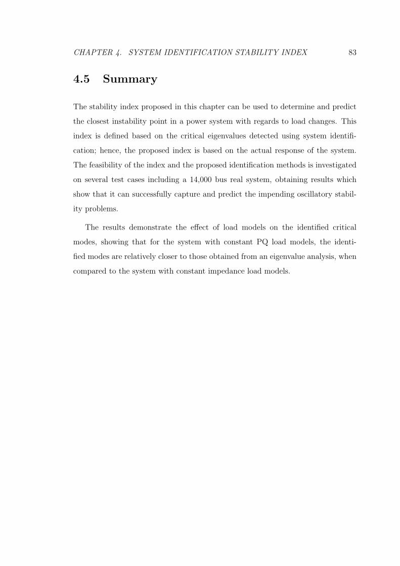
CHAPTER 4. SYSTEM IDENTIFICATION STABILITY INDEX 83
4.5 Summary
The stability index proposed in this chapter can be used to determine and predict
the closest instability point in a power system with regards to load changes. This
index is defined based on the critical eigenvalues detected using system identifi-
cation; hence, the proposed index is based on the actual response of the system.
The feasibility of the index and the proposed identification methods is investigated
on several test cases including a 14,000 bus real system, obtaining results which
show that it can successfully capture and predict the impending oscillatory stabil-
ity problems.
The results demonstrate the effect of load models on the identified critical
modes, showing that for the system with constant PQ load models, the identi-
fied modes are relatively closer to those obtained from an eigenvalue analysis, when
compared to the system with constant impedance load models.

Chapter 5
Damping Torque Index
5.1 Introduction
The main obstacle for the stability index SISI in the preceding chapter, as well
as with similar off-line indices, is identifying the critical modes in advance, which
is not an easy task in some systems. Therefore, in this chapter, another index is
proposed, which is also based on the time-domain response, and hence of use in
on-line stability monitoring. The new index is defined based on damping torque
concepts for the individual generators.
The theoretical background on damping and synchronizing torques is first pre-
sented, and the procedure to derive the damping and synchronizing coefficients
from a linearized model (LM) of the power system is described. Then, the iden-
tification techniques used to estimate the damping coefficient from the transient
response of the system are explained. The results of applying the proposed identi-
fication methods to calculate the damping torque coefficient are also presented and
discussed for a variety of test cases, focusing on the behavior of this coefficient as
84

CHAPTER 5. DAMPING TORQUE INDEX 85
a stability/security index. Finally, damping torque estimation from ambient data
is discussed and an effective identification method is proposed.
5.2 Damping and Synchronizing Torque
The concept of damping and synchronizing torques for a single-machine-infinite-
bus (SMIB) system was first introduced in [35]. Thus, electromechanical torque
Te deviations of a machine can be expressed in terms of its speed ω and angle δ
deviations, known as damping and synchronizing torque, respectively. The damping
and synchronizing torques are the in time phase components proportional to the
speed and angle deviations [64], and are defined as:
∆Te(t) = Kd ω0 ∆ω(t)︸ ︷︷ ︸
damping
+ Ks ∆δ(t)︸ ︷︷ ︸
synchronizing
(5.1)
or in the frequency domain:
∆Te(s) = (Kd +Ks
s) ω0 ∆ω(s) (5.2)
where Kd (p.u./rad/sec) and Ks (p.u.) are damping and synchronizing coefficients,
respectively; and ω0 (rad/sec) is the system angular frequency. The generator’s
angle and speed deviations in (5.1) are typically measured with respect to a center
of inertia (COI ), i.e. δi = δi − δCOI and ωi = ωi − ωCOI , where
δCOI =1
MT
g∑
i=1
Miδi (5.3)
ωCOI =1
ω0
dδCOI
dt
and MT =∑g
i=1 Mi is the total inertia of the g generators.

CHAPTER 5. DAMPING TORQUE INDEX 86
Since ω0∆ω(t) = d∆δ(t)/dt, or in discrete form ω0∆ω[k] = (∆δ[k] − ∆δ[k − 1])/Ts,
where Ts is the sampling time, one can rewrite (5.1) as:
∆Te[k] = ξ ∆δ[k − 1] + ζ ∆δ[k] (5.4)
where ξ = −Kd/Ts and ζ = Kd/Ts + Ks. Equation (5.4) can be used to calculate
ξ and ζ from sampled signals, thus yielding Kd and Ks. Using (5.4), which only
requires two signals Te and δ, as opposed to (5.1), which requires three signals Te,
ω and δ, reduces the errors due to mean value and low frequency trends in the
measured signals, due to the effect of the governor’s response.
For a single-machine-infinite-bus (SMIB) system, the synchronizing and damp-
ing coefficients correctly define the frequency and damping of the electromechanical
mode. However, for a multi-machine power system, the electromechanical oscilla-
tions contain different modes, and hence a single mode cannot simply be assigned
to a single machine [65], since the oscillations of each machine are a linear combi-
nation of all the modes. Hence, in this case, one must be aware that the damping
coefficient of a given machine includes the effect of several modes.
5.2.1 Damping and Synchronizing Coefficients
In the linear model (4.3), let assume that only the ith mode of the system λi =
αi + jβi is excited by an initial condition x0 in the direction of right eigenvector Ui
associated with λi. Hence, any output yk(t) can be expressed as yk(t) = CkUieλit,
or yk(s) = CkUi/(s − λi) where Ck is the kth row of C. In this case, one may write
the following relationship between the speed and electrical torque of machine j,
defined as Dj:
Dj =∆Tej
(t)
∆ωj(t)=
∆Tej(s)
∆ωj(s)=
CTejUi
CωjUi
(5.5)
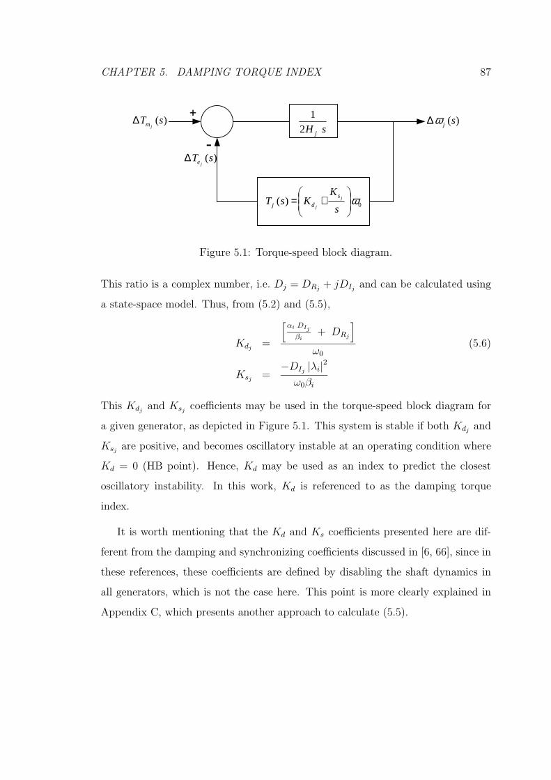
CHAPTER 5. DAMPING TORQUE INDEX 87
sH j21+
-
)(sTjm∆
)(sTje∆
)(sjω∆
0)( ω
+=
s
KKsT j
j
s
dj
Figure 5.1: Torque-speed block diagram.
This ratio is a complex number, i.e. Dj = DRj+ jDIj
and can be calculated using
a state-space model. Thus, from (5.2) and (5.5),
Kdj=
[αi DIj
βi+ DRj
]
ω0
(5.6)
Ksj=
−DIj|λi|2
ω0βi
This Kdjand Ksj
coefficients may be used in the torque-speed block diagram for
a given generator, as depicted in Figure 5.1. This system is stable if both Kdjand
Ksjare positive, and becomes oscillatory instable at an operating condition where
Kd = 0 (HB point). Hence, Kd may be used as an index to predict the closest
oscillatory instability. In this work, Kd is referenced to as the damping torque
index.
It is worth mentioning that the Kd and Ks coefficients presented here are dif-
ferent from the damping and synchronizing coefficients discussed in [6, 66], since in
these references, these coefficients are defined by disabling the shaft dynamics in
all generators, which is not the case here. This point is more clearly explained in
Appendix C, which presents another approach to calculate (5.5).

CHAPTER 5. DAMPING TORQUE INDEX 88
5.2.2 Electromechanical Mode Estimation
The characteristic equation corresponding to the block diagram depicted in Figure
5.1 can be mathematically expressed as
2Hj
ω0
s2 + Kdjs + Ksj
= 0 (5.7)
The roots of the characteristic equation may be used to estimate the damping and
the frequency of the electromechanical mode. Although this is true if oscillations
consist of only one mode, it may still be used when several modes are present but
one is more dominant. However, the estimates in this case will not be accurate
due to under-parameterization of a system of order n ≥ 2 when represented by a
second order system. Thus, if several strong modes are dominant in the response,
in order to correctly capture all of the modes, the linear parametric models, such
as the ARMA model or the state-space model explained in Chapter 3, have to be
employed instead.
The main application of using Kd, as explained before, is predicting the available
stability margin without the need to monitor certain modes. However, it can also be
used to provide information about the poorly damped local or sometimes inter-area
modes, and hence re-tuning the controllers such as PSSs.
5.3 Techniques
5.3.1 Ordinary Least Square (OLS)
Damping and synchronizing coefficients in (5.1) can be estimated using an ordinary
least square (OLS) method [64]. It is basically a fitting problem which can be

CHAPTER 5. DAMPING TORQUE INDEX 89
described as:
Y = [Ω ∆] K + ǫ (5.8)
= X K + ǫ
where Y =[Te[1] Te[2]... Te[N ]]T ∈ ℜN ; Ω = ω0 [∆ω[1] ∆ω[2]... ∆ω[N ] ]T ∈ ℜN ;
∆ =[∆δ[1] ∆δ[2]... ∆δ[N ]]T ∈ ℜN ; ǫ ∈ ℜN represents “residuals” introduced to
account for fitting errors and measurement noise; K = [Kd Ks]T ; and N is the
number of samples. The ordinary least square estimate can be obtained as:
KOLS = (XT X)−1XT Y. (5.9)
Here, KOLS is unbiased, efficient (or Markov estimate), and consistent when ǫ is
white noise with zero mean [67]. Furthermore, it is also identical to the maximum
likelihood estimator when ǫ is normally distributed. However, the condition of
whiteness for the current application is not guaranteed, thus K might be biased.
This will be clearly shown here in a number of case studies.
5.3.2 Generalized Least Square (GLS)
From the system identification point of view, (5.8) can be represented as follows:
y[k] = x[k] K + H(q) e[k] (5.10)
where e[k] is white noise, H−1(q) is a whitening filter, and q is the shifting operator
defined by q−1y[k] = y[k − 1].
Selecting a proper candidate model set in this case, which includes the true
model, is an essential aspect to obtain accurate parameter estimates. On the other
hand, over-parameterization can lead to high computational costs as well as numer-
ical problems (e.g. convergence and local minima). Therefore, one should search
CHAPTER 5. DAMPING TORQUE INDEX 90
for a model set that includes the true model with as low number of parameters as
possible. It is also important to consider that choosing a rather simple model, i.e.
under-parameterization, might lead to inaccurate parameter estimates [59].
The candidate model (5.10) with H(q) = 1, which leads to (5.9), is not a general
model and may not correctly represent the power system dynamics. For example,
when the perturbations are large and hence the linearity assumption does not hold,
the OLS estimates can lead to erroneous results. Experience shows that by adding
a transfer function such as H(q) = 1/(1 + h1q−1 + h2q
−2 + ... + hpq−p) with p = 1
or 2, good results can be obtained [67]. This method is also known as generalized
least square (GLS) and can be used to correctly model the residuals or filter the
nonlinear effects. In this case, K along with the parameters of the whitening filter
are denoted as θ, and are estimated using PEMs. These methods are basically
based on an optimization problem such as:
Min V (θ) =1
N
N∑
k=1
1
2ǫ2[k] (5.11)
s.t. ǫ[k] = H−1(q) y[k] − x[k] K
5.3.3 Robust Fitting with Bisquare Weights (RFBW)
Robust fitting may also be employed as another remedial method for handling the
nonlinear effects, which can occur due to large deviations from an operating point.
This method is basically an iterative weighted least square (WLS) method, and is
able to give different weights to each residues during the fitting process; data with
lower quality are given less weight, since the part of the signal that is distorted due
to the nonlinear effects is hard to fit, and hence should be less important in the
estimation process. One may consider using small perturbations as a way to avoid

CHAPTER 5. DAMPING TORQUE INDEX 91
nonlinearities; however, in the current application, small disturbances may not be
feasible, since the perturbations have to be large enough to be distinguished from
measurement noise.
Robust fitting employs the following objective function, which assigns weights
to different predicted errors:
Min V =1
N
N∑
k=1
wk ǫ2[k] (5.12)
The estimated damping and synchronizing coefficients in this case are:
KWLS = (XT W X)−1XT W Y. (5.13)
where W = diagw1, w2, ... , wN ∈ ℜN×N . There are different weights which can
be utilized in the objective function (5.12) [68]; in this work, bisquare weights are
used. This method has been previously used in economics to decrease the sensitivity
of least square to “extreme” values called outliers.
5.4 Damping Torque Estimation from Transient
Response
For various test cases, the damping torque index is calculated here by means of the
previously mentioned techniques. Similar to the eigenvalue index SISI, the feasi-
bility of using Kd for different types of signals known as ringdown data (transient
response) or ambient data (noise) is addressed. The signals are recorded with the
same specifications mentioned for the eigenvalue index SISI; however, in addition
to the generator power signal, generator angle or speed have to be measured. The
behavior of the index, as the system loading changes, is depicted for each case,
illustrating its capability to predict the closest stability margin.

CHAPTER 5. DAMPING TORQUE INDEX 92
The electromechanical torque and generator angle of each generator following
a large disturbance, such as a line outage or a three phase fault, are recorded so
that it contains at least three periods of oscillations. Then, the measurement noise
is removed with a Chebyshev low pass filter with a cut off frequency of 2 Hz, and
then re-sampling the signal at 10 Hz. The mean and low frequency trends of the
measured signal have to be also removed.
5.4.1 Single-Machine-Infinite-Bus (SMIB)
The generator in the simple test system depicted in Figure 2.7 was modeled using a
subtransient model. There is an electromechanical mode, which moves toward the
RHP, as the load increases from 100 MW to 700 MW, resulting in an increase in
tie-line power as well as a gradual decrease in the generator’s damping coefficient
Kd. The results obtained for “theoretical” and estimated values of Kd are shown
in Figure 5.2; observe that all the identification methods were able to correctly
calculate Kd. However, for heavy loads, the different values for Kd obtained from
the various methods used coincide, which is to be expected, since at light loading
conditions the mode is well-damped. This is akin to the case when eigenvalues are
to be identified using the time-domain response of the system, as reported in [23].
5.4.2 Two-area Benchmark System
The single line diagram of the two-area benchmark system used here is shown
in Figure 2.10. There is an inter-area mode and two local modes that change
as the loads are increased. Depending on the load and dispatch scenarios, one
could expect to have different eigenvalue profiles. For instance, in this system, two
dispatch scenarios, Schedules 1 and 2, result in fairly different eigenvalue profiles,

CHAPTER 5. DAMPING TORQUE INDEX 93
100 200 300 400 500 600 700−0.02
−0.01
0
0.01
0.02
0.03
0.04
0.05
0.06
0.07
Loading (MW)
Kd (
p.u
./ra
d/s
)
LMOLSGLSRFBW
Figure 5.2: Damping coefficient Kd from transient response for the SMIB.
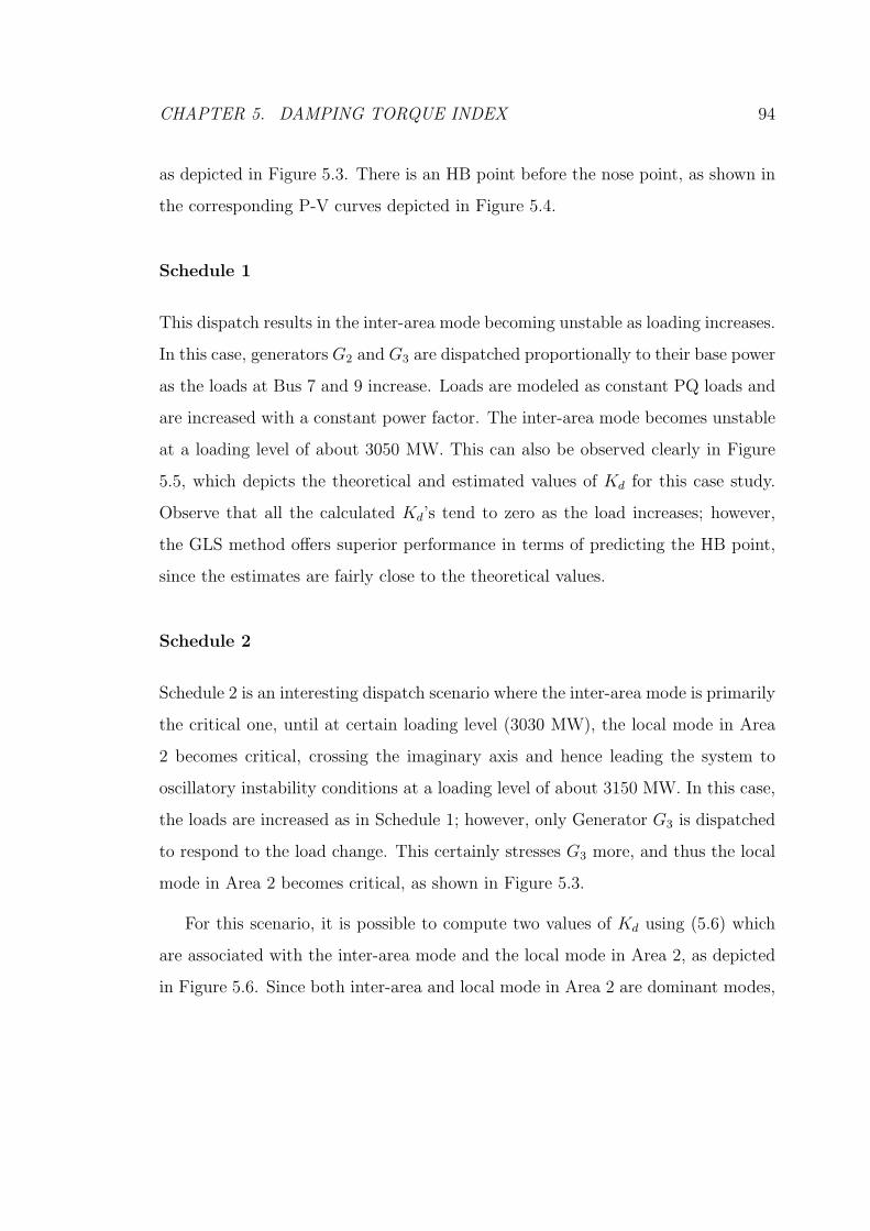
CHAPTER 5. DAMPING TORQUE INDEX 94
as depicted in Figure 5.3. There is an HB point before the nose point, as shown in
the corresponding P-V curves depicted in Figure 5.4.
Schedule 1
This dispatch results in the inter-area mode becoming unstable as loading increases.
In this case, generators G2 and G3 are dispatched proportionally to their base power
as the loads at Bus 7 and 9 increase. Loads are modeled as constant PQ loads and
are increased with a constant power factor. The inter-area mode becomes unstable
at a loading level of about 3050 MW. This can also be observed clearly in Figure
5.5, which depicts the theoretical and estimated values of Kd for this case study.
Observe that all the calculated Kd’s tend to zero as the load increases; however,
the GLS method offers superior performance in terms of predicting the HB point,
since the estimates are fairly close to the theoretical values.
Schedule 2
Schedule 2 is an interesting dispatch scenario where the inter-area mode is primarily
the critical one, until at certain loading level (3030 MW), the local mode in Area
2 becomes critical, crossing the imaginary axis and hence leading the system to
oscillatory instability conditions at a loading level of about 3150 MW. In this case,
the loads are increased as in Schedule 1; however, only Generator G3 is dispatched
to respond to the load change. This certainly stresses G3 more, and thus the local
mode in Area 2 becomes critical, as shown in Figure 5.3.
For this scenario, it is possible to compute two values of Kd using (5.6) which
are associated with the inter-area mode and the local mode in Area 2, as depicted
in Figure 5.6. Since both inter-area and local mode in Area 2 are dominant modes,
CHAPTER 5. DAMPING TORQUE INDEX 95
−1.2 −1 −0.8 −0.6 −0.4 −0.2 0 0.2
8
8.2
8.4
8.6
(c): Local mode − Area 2
Ima
g (
rad
/s)
−0.3 −0.2 −0.1 0 0.1 0.2
4
4.5
5
5.5
Ima
g (
rad
/s)
(a): Inter−area mode
−1.1 −1 −0.9 −0.8 −0.7 −0.6 −0.5
7
7.2
7.4
7.6
Ima
g (
rad
/s)
(b): Local mode − Area 1
* : Schedule 1
: Schedule 2
: Schedule 1
: Schedule 2
: Schedule 1
: Schedule 2
o
* o
* o
Real (sec−1)
Figure 5.3: Eigenvalue profiles for different dispatch scenarios; Schedules 1 and 2.

CHAPTER 5. DAMPING TORQUE INDEX 96
2800 2900 3000 3100 3200 3300 3400 3500 3600 3700 38000.92
0.93
0.94
0.95
0.96
0.97
0.98
0.99
1
Loading (MW)
V7 (
p.u
.)
Schedule 1Schedule 2
HB
*
*HB
Figure 5.4: P-V curves at Bus 7 for the 2-area benchmark system.

CHAPTER 5. DAMPING TORQUE INDEX 97
2000 2500 3000 3500−0.01
0
0.01
0.02
0.03
0.04
Kd (p
.u./
rad
/s)
Loading (MW)
G1
LM: Inter−area modeOLSGLSRFBW
2000 2500 3000 3500−0.01
0
0.01
0.02
0.03
0.04
Kd (p
.u./
rad
/s)
Loading (MW)
G2
2000 2500 3000 3500−0.01
−0.005
0
0.005
0.01
0.015
0.02
Kd (p
.u./
rad
/s)
Loading (MW)
G3
2000 2500 3000 3500−0.02
−0.01
0
0.01
0.02
0.03
0.04
0.05
Kd (p
.u./
rad
/s)
Loading (MW)
G4
Figure 5.5: Damping coefficients of all generators obtained from transient response
for the 2-area benchmark system for Schedule 1.

CHAPTER 5. DAMPING TORQUE INDEX 98
time-domain simulation results in this case would be influenced by both of them,
and so would be the identified Kd’s. Notice that in this case, the values obtained
for Kd from OLS are not accurate; neither are the predicted stability margins. On
the other hand, the Kd’s obtained using GLS present the best results in terms of
accuracy in estimation as well as prediction. The RFBW’s accuracy is between the
OLS and GLS, and from the computational point of view, it is slower than OLS
and faster than the GLS. The advantage of using Kd, when compared to eigen-
value based indices, is that, in order to monitor system stability/security margin,
the damping coefficient is able to provide accurate margins without the need for
monitoring particular modes. This can be an issue for eigenvalue-based indices.
For instance, the damping torque is able to capture the oscillatory phenomenon for
both schedules; on the other hand, for Schedule 2, if only the inter-area mode were
used as an index, it would yield inaccurate margins.
5.4.3 Real System (14,000 buses)
There are around 2000 generators and 22 areas in this system, and hence only the
slack generators in some areas are monitored. The areas are selected by looking at
the mode shape corresponding to the critical mode. The critical mode moves to the
RHP with respect to load change, resulting in unstable oscillations triggered by a
line outage as shown in Figure 5.7. Figure 5.8 depicts the Kd for the slack buses in
four different areas where the critical mode is highly observable. Observe that only
some of the generators are able to successfully predict the oscillatory phenomenon,
indicating the importance of employing several monitoring units in different parts
of the system.

CHAPTER 5. DAMPING TORQUE INDEX 99
2400 2600 2800 3000 3200 3400
−0.02
0
0.02
0.04
0.06
0.08
Kd (p
.u./
rad
/s)
Loading (MW)
G1
LM:Inter−area modeLM:Local mode Area−2OLSGLSRFBW
2400 2600 2800 3000 3200 3400
−0.02
0
0.02
0.04
0.06
0.08
Kd (p
.u./
rad
/s)
Loading (MW)
G2
2400 2600 2800 3000 3200 3400
−0.02
0
0.02
0.04
Kd (p
.u./
rad
/s)
Loading (MW)
G3
2400 2600 2800 3000 3200 3400
−0.02
0
0.02
0.04
0.06
0.08
Kd (p
.u./
rad
/s)
Loading (MW)
G4
Figure 5.6: Damping coefficients of all generators obtained from transient response
for the 2-area benchmark system for Schedule 2.

CHAPTER 5. DAMPING TORQUE INDEX 100
010
2030
4050
60
0
10
20
30
4059.975
59.98
59.985
59.99
59.995
60
60.005
60.01
60.015
Time (sec)K: Area Number
Sla
ck G
en
era
tor
GK S
pe
ed
(H
z)
Figure 5.7: Generator speed oscillations due to the trigger of the unstable elec-
tromechanical mode in the 14,000-bus real system.

CHAPTER 5. DAMPING TORQUE INDEX 101
38.6 38.7 38.8 38.9 39 39.1 39.2 39.3 39.4 39.5 39.6
0
0.2
0.4
0.6
0.8
1
Loading (MW)
No
rma
lize
d
Kd
LMG
A1
GA
2G
A3
GA
4
GA
j
: Slack Generator in Area j
Figure 5.8: Damping coefficients of slack generators in different areas for the 14,000-
bus real system.

CHAPTER 5. DAMPING TORQUE INDEX 102
5.5 Damping Torque Estimation from Ambient
Data
For the following test cases, it is assumed that the system is persistently being
excited by random load switching, and hence the measured signal of the system is
a colored noise. The advantage of using this kind of signals is twofold: There is no
need to carry on expensive, risky, intrusive tests; second, the linearity assumption
due to the small magnitude of the perturbations holds.
5.5.1 Box-Jenkins Model
Experience shows that RFBW yields results similar to OLS, because the pertur-
bations are small, and the problem of nonlinear effects does not show up in the
measured response. However, due to the persistent excitation of different modes,
the whitening filter in this case is more complicated.
As explained in Section 5.3.2, for the transient response of the system, GLS is
used to model the correlated residuals; notice that the residuals were modeled by
means of an AR(p). Since the objective is to obtain white ǫ[k], and considering the
fact that the first term on the right side of (5.10) (x[k] K) cannot be changed, it
would be beneficial to use a Box-Jenkins model. This model provides a parametric
model with errors being modeled separately from the first term that is related to
the system dynamics. The error term properties are modeled by a rational transfer
function H(q) with both numerator and denominator; thus, (5.10) can be written

CHAPTER 5. DAMPING TORQUE INDEX 103
as:
y[k] = x[k] K + H(q) e[k] (5.14)
H(q) =1 + c1 q−1 + c2 q−2 + . . . + cnc
q−nc
1 + d1 q−1 + d2 q−2 + . . . + dndq−nd
(5.15)
This model is known as a Box-Jenkins (BJ) model and is denoted by BJ(nc,nd). The
BJ model in this case is indeed employing an ARMA(nc,nd) in order to correctly
model the residuals. The orders nc and nd can be selected by means of AIC or
FPE. For instance, the FPE can be computed as:
FPE = V (θ)1 − κ
N
1 + κN
(5.16)
where θ = [KT c1 c2 ... cncd1 d2 ... dnd
]T and κ = dim(θ). It is worth mentioning
that for large data blocks, i.e. N −→ ∞, the FPE is the same as the loss function
V (θ), which is the case for ambient data; and therefore, V (θ) can be used instead
of FPE.
5.5.2 Two-area Benchmark System-Schedules 1 and 2
For the 2-area benchmark system explained in detail in Section 5.4.2, two previously
defined dispatch scenarios (Schedules 1 and 2) are investigated, where 1% of the
loads at Buses 7 and 9 are being switched as driving noise. The BJ(nc,nd) model for
each case is utilized to estimate the damping torque; the optimum order is selected
by inspecting the loss function of models for a given range of nc and nd. First,
a range is selected for nc and nd, thus resulting in models with different orders;
for each case, the corresponding BJ model as well as the loss function V (θ) are
then estimated. Usually, as the order is increased, after a certain point which is
related to the optimum order, no significant reduction in V (θ) is achieved. The

CHAPTER 5. DAMPING TORQUE INDEX 104
parsimony principle [58] has to also be taken into consideration, which suggests
selecting the simplest model of all the models that can accurately describe a system.
Furthermore, from an optimization point of view, adding more MA terms results
in more complexity and nonlinearity, as the corresponding regressor is not linear;
thus, parameter estimation would be significantly easier for smaller nc’s.
For instance, Figures 5.9 and 5.10 suggest BJ(1,2) for Schedule 1, and BJ(2,5)
for Schedule 2. Only an inter-area mode is dominant for Schedule 1, as opposed
to Schedule 2; consequently, Schedule 1 needs a simpler model to describe the
residuals.
The predicted errors ǫ[k] may also be examined to check the whiteness assump-
tion, which in turn, leads to efficient estimates as explained in Section 5.3.1. The
typical whiteness test is inspecting the sample autocorrelation function ACF (rǫ[τ ]),
i.e. for ǫ[k] to be white, rǫ[τ ] = 0 for τ 6=0. Usually, the standard deviations obtained
via Barttlet’s approximation [69] are used to test the hypothesis, i.e. the whiteness
is rejected if the sample rǫ[τ ] falls out of the, for instance, 95% confidence interval.
For a selected model, if the whiteness test indicates that ǫ[k] is correlated, then one
needs to reexamine the model and data, and search for a statistically better model.
A close inspection of the ACF for both schedules demonstrate the ability of
using BJ models in obtaining white residuals as depicted in Figures 5.11 and 5.12.
As well, the confidence interval of the estimated Kd’s must be checked to ensure
that it does not experience a significant increase, as the order of the filter H(q)
increases. For instance, in Schedule 1, the standard deviation of the Kd and Ks
for various filter models are depicted in Figure 5.13, showing that the standard
deviation of the Kd for the selected model, BJ(1,2), is relatively close to that of the
BJ(0,0) or OLS.

CHAPTER 5. DAMPING TORQUE INDEX 105
02
46
810
0
5
10
0
0.5
1
1.5
2
x 10−3
nc
nd
V (
θ )
Figure 5.9: Loss function for the BJ(nc,nd) model in the 2-area benchmark system;
Schedule 1.

CHAPTER 5. DAMPING TORQUE INDEX 106
0
5
10
02
46
810
1.95
2
2.05
2.1
2.15
2.2
2.25
x 10−3
nc n
d
V (
θ )
Figure 5.10: Loss function for the BJ(nc,nd) in the 2-area benchmark system; Sched-
ule 2.

CHAPTER 5. DAMPING TORQUE INDEX 107
0 2 4 6 8 10 12 14 16 18 20−0.5
0
0.5
1
Lag time
AC
F
0 2 4 6 8 10 12 14 16 18 20−0.5
0
0.5
1
Lag time
AC
F
BJ(0,0) or OLS
BJ(1,2)
Figure 5.11: Whiteness test for the OLS and BJ(1,2) models using ACF(ǫ[k]) in
the 2-area benchmark system; Schedule 1. Horizontal bars indicate 95% confidence
intervals.

CHAPTER 5. DAMPING TORQUE INDEX 108
0 2 4 6 8 10 12 14 16 18 20−0.5
0
0.5
1
Lag time
AC
F
0 2 4 6 8 10 12 14 16 18 20−0.5
0
0.5
1
Lag time
AC
F
BJ(0,0) or OLS
BJ(2,5)
Figure 5.12: Whiteness test for the OLS and BJ(2,5) models using ACF(ǫ[k]) in
the 2-area benchmark system; Schedule 2. Horizontal bars indicate 95% confidence
intervals.

CHAPTER 5. DAMPING TORQUE INDEX 109
BJ(0,0)
BJ(0,1)
BJ(1,0)
BJ(1,1)
BJ(1,2)
BJ(0,5)
K_s
K_d
0
0.005
0.01
0.015
0.02
0.025
Sta
nd
ard
de
via
tio
n o
f K
d &
Ks
Figure 5.13: The standard deviation of estimated Kd and Ks for the BJ(nc,nd)
model; Schedule 1.

CHAPTER 5. DAMPING TORQUE INDEX 110
The estimated Kd’s for both schedules are shown in Figures 5.14 and 5.15. A
BJ model is employed to estimates the Kd for each generator and is compared to
the theoretical and OLS estimates.
Observe that for Schedule 1, all the calculated Kd’s tend to zero as the load in-
creases; however, the BJ method offers superior performance in terms of predicting
the HB point as well as providing fairly close estimates to the theoretical values,
which are denoted as LM in Figure 5.14. Notice that the OLS underestimates the
Kd for all the generators, especially at light loading levels.
For Schedule 2, only some of the estimated Kd’s are able to predict the instability
point. For instance, the trend of the Kd’s of generators G1 and G2 are giving better
prediction of the instability point compared to the Kd’s of the Generators G3 and
G4. Notice that the OLS is providing erroneous Kd’s for Generators G3 and G4,
and that it is unable to predict the instability point, demonstrating the need for
using better models such as a BJ model.
The differences observed for generators in Schedule 2 are because of the mag-
nitude of the modes’ observability on each generator, i.e. the more observable a
mode on a generator, the larger the corresponding oscillations on the generator’s
response. In Schedule 1, the critical mode is an inter-area mode, and therefore, its
observability is almost the same on all the generators; thus, the differences in Kd’s
are not significant, and all of them can be used to predict the oscillatory stability
limit. On the other hand, in Schedule 2, the local mode in Area 2 is not well ob-
served on the generators in Area 1, and therefore, when this mode becomes critical,
its effect in not significant on Area 1.

CHAPTER 5. DAMPING TORQUE INDEX 111
2000 2200 2400 2600 2800 3000−0.005
0
0.005
0.01
0.015
0.02
0.025
Kd (p
.u./ra
d/s
)
Loading (MW)
G1
LM: Inter−area modeOLSBJ(1,2)
2000 2200 2400 2600 2800 3000−0.005
0
0.005
0.01
0.015
0.02
0.025
Kd (p
.u./ra
d/s
)
Loading (MW)
G2
2000 2200 2400 2600 2800 3000−0.005
0
0.005
0.01
0.015
0.02
0.025
Kd (p
.u./
rad
/s)
Loading (MW)
G3
2000 2200 2400 2600 2800 3000−0.005
0
0.005
0.01
0.015
0.02
0.025
Kd (p
.u./
rad
/s)
Loading (MW)
G4
Figure 5.14: Damping coefficients of all generators from ambient data for the 2-area
benchmark system; Schedule 1.

CHAPTER 5. DAMPING TORQUE INDEX 112
2400 2600 2800 3000 32000
0.02
0.04
0.06
0.08
Kd (
p.u
./ra
d/s
)
Loading (MW)
G1
2400 2600 2800 3000 32000
0.02
0.04
0.06
0.08
Kd (
p.u
./ra
d/s
)
Loading (MW)
G2
2400 2600 2800 3000 32000
0.02
0.04
0.06
0.08
Kd (
p.u
./ra
d/s
)
Loading (MW)
G3
2400 2600 2800 3000 32000
0.02
0.04
0.06
0.08
Kd (
p.u
./ra
d/s
)
Loading (MW)
G4
LM: Inter-area modeLM: Local mode Area 2OLS or BJ(0,0)BJ(2,5)
Figure 5.15: Damping coefficients of all generators from ambient data for the 2-area
benchmark system; Schedule 2.

CHAPTER 5. DAMPING TORQUE INDEX 113
5.6 Summary
The procedure to derive the theoretical values of damping and synchronizing co-
efficients obtained using linearized models of power system is demonstrated. In
the systems with single dominant mode, the accuracy of the obtained coefficients
using system identification and measured time-domain response of the system is
investigated by comparing them with the theoretical values.
The GLS and RFBW identification methods are shown to be better alternatives
than the OLS method when the transient response of the power system is available.
In particular, it is shown that the OLS method may not be able to accurately esti-
mate the coefficients, because of the nonlinear effects that appear in the measured
response of a power system; these effects can be reduced using smaller perturba-
tions. There is a trade off, however, between the magnitude of the perturbation
and SNR of the measured signals, i.e. the lower the SNR, the less accurate the
estimates.
The damping coefficient is shown to be a useful index to predict the distance to
instability points when system loading changes. It is basically a close duplicate of
the electromechanical modes behavior; however, it does not require the monitoring
of certain modes, which can be an issue in large power systems. Hence, this index
may help system operators determine proximity to an oscillatory instability with-
out requiring modeling assumptions and simulations, thus allowing to take proper
actions in the case of contingencies and congestion problems.
The Box-Jenkins model is proposed to estimate the damping torque from am-
bient data, and its effectiveness and superior performance over OLS are illustrated
by means of several examples.

Chapter 6
Estimation of Uncertainty
6.1 Introduction
In parameter estimation, second order statistical properties of the estimates, such
as confidence intervals, are important when discussing the quality of the estimates,
i.e. the tighter the confidence intervals, the better the estimates. For the indices
presented in the preceding chapters, the mean value and the confidence interval
(standard deviation of the estimates) were studied to ensure that the estimates are
both accurate and dependable (e.g. Figures 4.20 and 4.22). The confidence inter-
vals, however, were obtained by means of a Monte-Carlo type of simulation, which
requires repeating the simulation for several realizations of the noise; hence, they
are computationally expensive and in some cases impractical. For example, in a
real power system, the system operating conditions as well as its dynamic charac-
teristics may change over a long time window due to load change, rescheduling, tap
changer operation, etc; hence, it is important to quickly conduct the experiment
to ensure that the system does not experience significant changes, and that the
114

CHAPTER 6. ESTIMATION OF UNCERTAINTY 115
stationarity assumption is not violated over the measurement time.
This chapter starts with a background on estimating the covariance of param-
eters of a linear parametric model. This information is useful in determining the
variance of the indices previously proposed.
The index proposed in Chapter 4, the SISI, has however a nonlinear relation-
ship with the parameters, and so does its variance. This nonlinear relationship is
due to the fact that the SISI is basically related to the eigenvalues of the system
that are the roots of the characteristic equation.
A technique that has been used in civil engineering for identification of civil
structures to establish a connection between the variance of parameters and the
variance of modal parameters is used here [70], and the corresponding equations
are explained in detail.
6.2 Covariance of Parameters
A linear model is given by
y(k) = G(q) u(k) + H(q) e(k) (6.1)
where y(k) is the output; u(k) is the input; and e(k) models the disturbances.
One-step-ahead prediction y(k|θ) uses the observations available up to time k − 1
to predict y(k), thus:
y(k|θ) = H−1(q) G(q) u(k) + [1 − H−1(q)] y(k) (6.2)

CHAPTER 6. ESTIMATION OF UNCERTAINTY 116
This notation is adapted from [71] and is used to emphasize its dependence on the
parameter vector θ. Rewriting (3.14) using (6.1) and (6.2) results in:
θ = arg min V (θ) (6.3)
V (θ) =1
N
N∑
k=1
1
2ǫ2(k, θ)
ǫ(k, θ) = y(k) − y(k|θ)
where function V (θ) denotes the loss that results from the model in the fitting
process, and “arg min” means the minimization argument of the function V (θ).
Hence, at the solution point, the differentiation of V (θ) with respect to θ has to be
zero, i.e.:
V′
(θ) = 0 (6.4)
Thus, an iterative algorithm, such as Newton, is used to solve for θ by means of
the Taylor series expansion of (6.4) around θ∗:
0 ≈ V′
(θ∗) + V′′
(θ∗)(θ − θ∗) (6.5)
or
(θ − θ∗) = −[
V′′
(θ∗)]−1
V′
(θ∗) (6.6)
which requires the first derivative (gradient) and second derivative (Hessian). These
derivatives can be expressed as:
V′
(θ∗) = − 1
N
N∑
k=1
ψ(k, θ∗) ǫ(k, θ∗) (6.7)
V′′
(θ∗) =1
N
N∑
k=1
ψ(k, θ∗) ψT (k, θ∗) +1
N
N∑
k=1
ψ′
(k, θ∗) ǫ(k, θ∗) (6.8)
ψ(k, θ∗) = − d
dθǫ(k, θ)|θ=θ∗ =
d
dθy(k|θ)|θ=θ∗
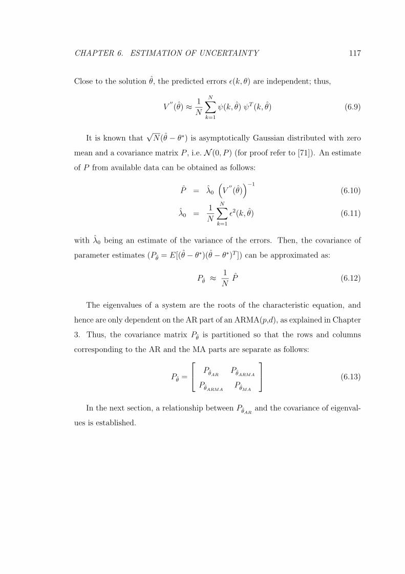
CHAPTER 6. ESTIMATION OF UNCERTAINTY 117
Close to the solution θ, the predicted errors ǫ(k, θ) are independent; thus,
V′′
(θ) ≈ 1
N
N∑
k=1
ψ(k, θ) ψT (k, θ) (6.9)
It is known that√
N(θ − θ∗) is asymptotically Gaussian distributed with zero
mean and a covariance matrix P , i.e. N (0, P ) (for proof refer to [71]). An estimate
of P from available data can be obtained as follows:
P = λ0
(
V′′
(θ))−1
(6.10)
λ0 =1
N
N∑
k=1
ǫ2(k, θ) (6.11)
with λ0 being an estimate of the variance of the errors. Then, the covariance of
parameter estimates (Pθ = E[(θ − θ∗)(θ − θ∗)T ]) can be approximated as:
Pθ ≈ 1
NP (6.12)
The eigenvalues of a system are the roots of the characteristic equation, and
hence are only dependent on the AR part of an ARMA(p,d), as explained in Chapter
3. Thus, the covariance matrix Pθ is partitioned so that the rows and columns
corresponding to the AR and the MA parts are separate as follows:
Pθ =
PθAR
PθARMA
PθARMAPθMA
(6.13)
In the next section, a relationship between PθARand the covariance of eigenval-
ues is established.

CHAPTER 6. ESTIMATION OF UNCERTAINTY 118
6.3 Covariance of Eigenvalues
Eigenvalues are related to the θAR, which are the coefficients of the characteristic
equation. This relationship can be written as:
Φ = γ(θAR) (6.14)
where γ(θAR) is a nonlinear function, and Φ denotes a vector containing the modal
parameters; for instance, the real part α and the frequency f of the eigenvalues can
be used to define:
Φ = [α1, f1, α2, f2, . . . , αp, fp]T ∈ ℜ2p (6.15)
In order to obtain the mean and variance of modal parameters, the expected
value operator may be applied to a Taylor series expansion of the function γ about
an operating point (Φ, θAR), which may be written as:
Φ ≈ Φ + J(θAR)(
θAR − θAR
)
(6.16)
J(θAR) =∂γ(θAR)
∂θAR
∣∣∣∣θAR=θAR
(6.17)
where J(θAR) ∈ ℜ2p×p.
Thus, rearranging (6.16) and applying the second moment operator (covariance)
yields
Cov Φ = E[
(Φ − Φ) (Φ − Φ)T]
= J(θAR) P (θAR) JT (θAR) (6.18)
This clearly shows the connection between the covariance of estimates P (θAR) and
the covariance of eigenvalues Cov Φ. Hence, in order to obtain Cov Φ, one first
needs to calculate the numeric Jacobian J(θAR) as follows:
Jij(θAR) =γi(θAR + ∆θj) − γi(θAR − ∆θj)
2h(6.19)

CHAPTER 6. ESTIMATION OF UNCERTAINTY 119
where
∆θj =
0...
0
h
0...
0
←− j
and h is a small number, and P (θAR) can be estimated using (6.12).
6.4 Test case
The proposed method for estimating the standard deviation of the identified modes
is tested with the 2-area benchmark system. First, a Monte-Carlo type of simula-
tion with 150 trials is performed by running independent simulations, where 1% of
the loads at Buses 7 and 9 are represented as Gaussian noise; 4-minutes data blocks
of generator G1’s power output are recorded in each simulation. Then, the prepro-
cessed data blocks along with a PEM are employed to estimate the parameters of
an ARMA(10,5) model representing the power system transfer function.
The estimated standard deviation of both the real part and frequency of the
inter-area mode obtained using (6.18) is depicted in Figures 6.1 and 6.2, respec-
tively. Observe that the estimates track the results corresponding to the Monte-

CHAPTER 6. ESTIMATION OF UNCERTAINTY 120
Carlos simulation, and that the mean of the estimates depicted in both figures
show that it can provide good accuracy with a significantly reduced number of tri-
als. For instance, in Figure 6.1, the convergence speed of the estimates is nearly 3
to 4 times faster than the Monte-Carlo method, which is a significant reduction in
the monitoring time.
6.5 Summary
A procedure to calculate the second order statistical properties of the previously
proposed is presented and justified. It is based on a technique that employs the
Taylor series expansion to establish a connection between the variance of parame-
ters and the variance of eigenvalues. The presented technique can be used to avoid
Monte-Carlo type of analyses, thus resulting in a significant reduction in computa-
tional time, making the proposed indices and monitoring techniques more appealing
for real-time applications.

CHAPTER 6. ESTIMATION OF UNCERTAINTY 121
0 50 100 1500
0.01
0.02
0.03
0.04
0.05
0.06
0.07
0.08
No. of Monte−Carlo simulations
Sta
nd
ard
de
via
tion
of
αc (
sec−
1)
Monte−CarloEstimated standard deviationMean of the estimated standard deviation
Figure 6.1: Standard deviation of the real part of the identified critical mode
−0.1228±j4.7824 for the 2-area benchmark system using Monte-Carlo and equation
(6.18).

CHAPTER 6. ESTIMATION OF UNCERTAINTY 122
0 50 100 1500
0.002
0.004
0.006
0.008
0.01
0.012
No. of Monte−Carlo simulations
Sta
nd
ard
de
via
tion
of f
c (H
z)
Monte−CarloEstimated standard deviationMean of the estimated standard deviation
Figure 6.2: Standard deviation of the frequency of the identified critical mode
−0.1228±j4.7824 for the 2-area benchmark system using Monte-Carlo and equation
(6.18).

Chapter 7
System Identification Techniques
Applied to Model Validation
7.1 Introduction
This chapter discusses the validation of the simplified models of major power system
elements, in particular synchronous generators and STATCOMs. These approxi-
mate models, instead of their detailed models, are typically used in power system
analysis packages, since power systems normally consist of several thousand buses
and machines, which may lead to intractable problem if full device models are used.
Thus, TS models are based on simplifications made to enhance computational effi-
ciency.
The validation procedure is performed by means of system identification applied
to the time-domain response of the both detailed models and simplified models,
so that the identified electromechanical modes can then be compared. The test
systems with detailed models was simulated in PSCAD/EMTDC program [72];
123

CHAPTER 7. SYSTEM IDENTIFICATION TECHNIQUES APPLIED TOMODEL VALIDATION 124
since large test cases cannot be handled in this program, the simulations were
obtained only for the IEEE 3-bus system.
7.2 Generator Modeling
As explained in Chapter 2, neglecting stator and network transients is the first
common step for simplification of the generator detailed model, as it provides a
very close approximation of the actual system response; this simplification along
with a few other assumptions result in the generator subtransient model [33], and
thus permit the use of a much larger step size for integration in transient stability
programs. The reason for neglecting stator and network transients is that these
transients are fast and damp quickly, as they are related to main frequency tran-
sients (50 Hz or 60 Hz), since when these transients are included, there will be a DC
offset term in the phase currents, which results in a DC braking torque and a main
frequency oscillatory torque, adding a slight degree of stability to the system [33].
Thus, the stability limits obtained using simplified models are conservative when
compared to the actual system stability limits. It has been shown that DC offset
currents can also develop abnormal oscillatory torques and back swing phenomena
[73, 74].
In order to compare generator models by means of system identification tech-
niques, the author has been forced to use signals generated through time-domain
simulations of detailed PSCAD/EMTDC [72] models for a small IEEE 3-bus system,
so that the resulting signals would be as close to field measurements as possible.
To perturb the system in PSCAD, a pseudo-random binary signal (PRBS) [75],
which approximates white noise, was used to represent a 1% load modulation at
Bus 3. The stochastic subspace technique applied to the generators’ output power

CHAPTER 7. SYSTEM IDENTIFICATION TECHNIQUES APPLIED TOMODEL VALIDATION 125
900 1000 1100 1200 1300 1400 1500 1600 1700 18000
0.1
0.2
0.3
0.4
0.5
0.6
Loading (MW)
SIS
I (se
c −1 )
EVIIdentification applied to measured PSCAD output
Figure 7.1: SISI for the IEEE 3-bus system; generator detailed model versus its
subtransient model.
yielded the results shown in Figure 7.1. Observe that both the generator detailed
model and its linearized subtransient model in PST yeild fairly similar results. The
maximum error in this case, between the identified and modeled SISI is 0.047 sec−1,
which is small.
The effect of including/or neglecting stator and network transients for small-
disturbance stability analyses and their impact on rotor angle mode was also stud-
ied. A small-disturbance stability program MASS [76], which is capable of per-
forming modal analysis including/neglecting network transients, was used for some
test cases and the results were given in Table 7.1. Observe that the corresponding

CHAPTER 7. SYSTEM IDENTIFICATION TECHNIQUES APPLIED TOMODEL VALIDATION 126
Table 7.1: Effect of including/neglecting network transients on the critical mode
Network Transients Included Neglected
Mode, Damping Mode, Damping
IEEE 3-bus -0.6509 ± j8.09, 8.01% -0.6298± j8.14, 7.71%
IEEE 14-bus -0.2502 ± j8.85, 2.82% -0.2158± j8.83, 2.44%
Two-area 11-bus -0.0940± j4.61 , 2.04% -0.0800± j4.61, 1.74%
eigenvalues indicate that network transients add a slight degree of stability to the
electromechanical mode, i.e. generator subtransient models are slightly conservative
from the point of view of calculating the electromechanical modes.
7.3 STATCOM Modeling
Readily available power system packages employ power flow or TS models to rep-
resent FACTS controllers. TS models, however, need to be validated from the
small-disturbance analysis point of view prior to using them in TS studies. This
can be achieved by means of system identification.
A typical STATCOM TS model is based on a fundamental frequency representa-
tion (phasor model) of the power system. In [1, 40], the authors study the accuracy
of the proposed TS model with regards to the detailed model only by means of
time-domain simulations. However, since these controllers can play a major role in
damping electromechanical oscillations [15, 31], one needs to validate these models
by means of small-disturbance stability analysis or modal analysis.
In this section, besides time-domain simulation results, a system identification
technique is used to investigate the accuracy of a typical STATCOM TS model

CHAPTER 7. SYSTEM IDENTIFICATION TECHNIQUES APPLIED TOMODEL VALIDATION 127
Table 7.2: STATCOM static data
Rc (Ω) Rtransformer (Ω) Xtransformer (Ω) C (µF)
200 0 0.108 740
Table 7.3: STATCOM controller parameters
KpαKIα
KpmKIm
Tw (s)
0.06 0.6 10 100 10
compared to its detailed model, from the small-disturbance stability analysis point
of view.
7.3.1 Test case
Both the STATCOM detailed and TS models are simulated in PSCAD/EMTDC
program. Due to the limitations imposed by PSCAD, only the IEEE 3-bus system
(Figure 2.8) is studied here. A 200 MVar STATCOM is connected to the Bus 3
through a coupling transformer (∆-Y, 6 kV/138 kV) to mainly regulate the voltage
at Bus 3. By adding a supplementary control loop (Figure 2.3), it could also be
used in damping oscillations. The data for the STATCOM are given in Tables 7.2
and 7.3.
The STATCOM detailed PSCAD model includes all the switches and the cor-
responding snubbers. The PWM control with a carrier frequency of 1260 Hz is
used to reduce the harmonics. It should be mentioned that the harmonic content
of the output voltage of the converter can be significantly reduced by increasing the
carrier frequency fc. The harmonics with order of Mfc ±Nfs appear in the output

CHAPTER 7. SYSTEM IDENTIFICATION TECHNIQUES APPLIED TOMODEL VALIDATION 128
voltage where fs is power system frequency, M and N are integers, and M + N
is an odd integer [77]; however, fc is limited to the maximum switching frequency
that the switches can withstand. A capacitor bank is connected to the Bus 3 to
filter high frequency harmonics; it is also providing 140 MVar of reactive power at
the fundamental frequency when the loading level is 900 MW.
For TS studies, the converter is replaced in PSCAD with a TS model based on a
controlled voltage source with a fixed frequency equal to the fundamental frequency
of the power system. The magnitude of the voltage source is determined from the
differential equation described in (2.7).
7.3.2 Standard Control Analysis
The detailed model and TS model are studied for several loading conditions. As
the load at Bus 3 increases, the electromechanical mode becomes less stable, as
shown in Table 7.4. The Prony method is employed to obtain the modal content
of the measured generator 1’s output power, showing a close agreement between
the eigenvalue calculated for the detailed and the TS models. The time-domain
simulation results for a line 2-3 outage and reconnection after 2 cycles are depicted in
Figure 7.2, showing fairly similar profiles. These results basically validate previous
studies of the STATCOM TS model [1, 40].
7.3.3 Supplementary Control Analysis
A supplementary control is added to damp the oscillations and remove the HB point.
The auxiliary signal used for this control is usually a local signal such as power or
current through the STATCOM adjacent lines. The auxiliary signal used here is

CHAPTER 7. SYSTEM IDENTIFICATION TECHNIQUES APPLIED TOMODEL VALIDATION 129
1 2 3 4 5 6 7 8 9 10350
400
450
PG
1
(M
W)
1 2 3 4 5 6 7 8 9 100.55
0.6
0.65
δ G1
(ra
d)
1 2 3 4 5 6 7 8 9 100.998
1
1.002
Time (sec)
ωG
1
(p
.u.)
Detailed modelTS model
Figure 7.2: The response of the system to a line 2-3 outage in the IEEE 3-bus
system; STATCOM at Bus 3 without supplementary control at 160% loading level.
CHAPTER 7. SYSTEM IDENTIFICATION TECHNIQUES APPLIED TOMODEL VALIDATION 130
Table 7.4: Critical electromechanical mode for the IEEE 3-bus system with STAT-
COM detailed and TS models.
Loading Level Detailed Model TS Model
Mode, Damping Mode, Damping
100% (900 MW) -0.5600± j8.11, 6.89% -0.5500± j8.11, 6.77%
130% (1170 MW) -0.3686 ± j8.12, 4.53% -0.3698± j8.11, 4.56%
160% (1440 MW) -0.1993 ± j8.08, 2.47% -0.2170± j8.07, 2.69%
190% (1710 MW) -0.0294 ± j8.02, 0.37% -0.0674± j8.00, 0.84%
the power in line 1-3 due to the better performance of power over other signals as
reported in [8]. At the same loading conditions as in the previous case, the critical
eigenvalue is calculated by means of the Prony method applied to the time-domain
simulation results. Table 7.5 and Figure 7.3 clearly illustrate the effectiveness of the
supplementary control in damping electromechanical oscillations when compared to
the results in Table 7.4; however, the calculated eigenvalues for the TS model in
this case are not as close to the ones related to the detailed model. Observe that
the TS model does a better job in damping oscillations, i.e. the TS model provides
more optimistic results from the eigenvalue analysis point of view, as depicted in
Figure 7.4. This basically results in an overestimation of the real stability margin
of the power system, and hence it is a potential risk in power system planning.
The discrepancy between the two models is better illustrated in Figure 7.5,
which shows the terminal voltage Vt, the DC bus voltage Vdc and converter’s delay
angle αconv. Observe that the fast transients during and right after clearing the
fault are not captured by the TS model. This is due to the fact that the TS model
was developed based on the balanced three phase voltages with fundamental fre-

CHAPTER 7. SYSTEM IDENTIFICATION TECHNIQUES APPLIED TOMODEL VALIDATION 131
Table 7.5: Critical electromechanical mode for the IEEE 3-bus system; STATCOM
with a supplementary control
Loading Level Detailed Model TS Model
Mode, Damping Mode, Damping
100% (900 MW) -0.9778± j8.51, 11.41% -1.0252± j8.44, 12.06%
130% (1170 MW) -0.7038 ± j8.72, 8.04% -0.8067± j8.63, 9.31%
160% (1440 MW) -0.4439 ± j8.76, 5.06% -0.5952± j8.66, 6.86%
190% (1710 MW) -0.1766 ± j8.70, 2.03% -0.3641± j8.60, 4.23%
quency, i.e. phasors, and hence is not able to capture the fast voltage transients.
The absorbed active and reactive power from the system to the converter depicted
in Figure 7.6 provide additional insights into the functioning of the different mod-
els. Notice that the active power, which plays a fundamental role in damping the
oscillating power ∆PG1, is larger in the case of the TS model, hence yielding a
more stable system. The main reason for this is that the TS model is based on
a controlled voltage source, with its magnitude being controlled by a differential
equation, whereas in the detailed model, the voltage is directly affected by fast DC
voltage transients.
7.4 Summary
The generator subtransient model and the STATCOM TS model are studied and
compared here with respect to their detailed models by means of PSCAD simula-
tions and system identification. From the electromechanical mode point of view,
the subtransient model of a generator yields very close results to the those obtained

CHAPTER 7. SYSTEM IDENTIFICATION TECHNIQUES APPLIED TOMODEL VALIDATION 132
1 2 3 4 5 6 7 8 9 10
380
400
420
PG
1
(M
W)
1 2 3 4 5 6 7 8 9 100.6
0.62
0.64
0.66
δ G1
(ra
d)
1 2 3 4 5 6 7 8 9 101
1.0005
1.001
Time (sec)
ωG
1
(p
.u.)
Without supplementary controlWith supplementary control
Figure 7.3: Detailed STATCOM model with and without a supplementary control
at a 130% loading level.

CHAPTER 7. SYSTEM IDENTIFICATION TECHNIQUES APPLIED TOMODEL VALIDATION 133
1 2 3 4 5 6 7 8 9 10350
400
450
PG
1
(M
W)
1 2 3 4 5 6 7 8 9 100.5
0.52
0.54
0.56
δ G1
(ra
d)
1 2 3 4 5 6 7 8 9 100.999
1
1.001
1.002
ωG
1
(p
.u.)
Detailed modelTS model
Figure 7.4: IEEE 3-bus system response for a line 2-3 outage for a STATCOM with
a supplementary control at 190% loading level.

CHAPTER 7. SYSTEM IDENTIFICATION TECHNIQUES APPLIED TOMODEL VALIDATION 134
1 2 3 4 5 6 7 8 9 10
0.88
0.9
0.92
Vt (
p.u
.)
1 2 3 4 5 6 7 8 9 1010
20
30
Vd
c (kV
)
1 2 3 4 5 6 7 8 9 10
0.7
0.75
0.8
0.85
Time (sec)
αco
nv (
De
g)
Detailed modelTS model
Figure 7.5: IEEE 3-bus system response for a line 2-3 outage for a STATCOM with
a supplementary control at a 190% loading level.
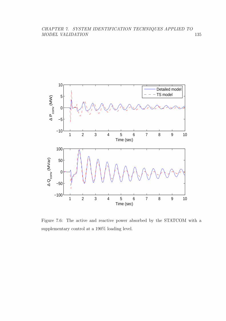
CHAPTER 7. SYSTEM IDENTIFICATION TECHNIQUES APPLIED TOMODEL VALIDATION 135
1 2 3 4 5 6 7 8 9 10−10
−5
0
5
10
Time (sec)
∆ P
con
v (M
W)
1 2 3 4 5 6 7 8 9 10−100
−50
0
50
100
Time (sec)
∆ Q
con
v (M
Va
r)
Detailed modelTS model
Figure 7.6: The active and reactive power absorbed by the STATCOM with a
supplementary control at a 190% loading level.

CHAPTER 7. SYSTEM IDENTIFICATION TECHNIQUES APPLIED TOMODEL VALIDATION 136
from the detailed model, while being slightly conservative, which is acceptable from
the planning point of view. On the other hand, the STATCOM TS model also yields
results fairly close to those of its detailed model for the case when no supplemen-
tary control is added to the STATCOM control. However, it is shown that, in
the presence of supplementary control, the STATCOM TS model gives optimistic
results regarding the electromechanical modes, which could be a problem for power
system operators and designers that has not been previously identified.
Chapter 8
Conclusions
8.1 Summary and Conclusions
This thesis concentrates on the study of oscillatory angle stability problems, propos-
ing system identification techniques to detect the electromechanical modes from
both power system transient response and ambient noise. Two on-line stability in-
dices, along with several identification methods, are proposed to monitor oscillatory
phenomena and to predict stability margins in a power system. Also, a procedure
is presented to obtain the confidence intervals of these stability indices from the
variance of the parameters. Finally, the generator subtransient model and a typical
STATCOM model are compared with respect to their detailed models using system
identification tools.
In Chapter 2, the models of some of the key power system components used in
this thesis are briefly explained. The importance of selecting the right models for
different kinds of power system analyses is also discussed. Power system stability
concepts, techniques and tools used throughout this thesis, such as voltage and
137

CHAPTER 8. CONCLUSIONS 138
angle stability, continuation power flow and system identification are presented
here as well.
Chapter 3 describes different types of signals that can be readily measured
in a power system, as well as the corresponding techniques to extract the signal
modal content. Namely, the Prony method is shown to be suitable for the transient
response with high SNR, while the LSMYW and the PEM are shown as proper
techniques to analyze ambient noise. A stochastic subspace identification method
is proposed to capture the critical modes of a power system from ambient data. The
asymptotic behavior of the proposed method is investigated by comparing it with
the PEM. It is shown that the methods are asymptotically equivalent; however, the
proposed method is easier to implement and is computationally more efficient.
Chapter 4 proposes an eigenvalue based index referred to as SISI to predict the
closest stability margin related to the impending oscillatory phenomena. Several
test cases along with a 14,000-bus power system are used to illustrate the effective-
ness of the index in practice.
In Chapter 5, another stability index based on the damping torque of individual
generators is proposed to overcome the shortcomings of the SISI, as it does not
require surveillance of certain modes. The drawback of using this index is that
the contributing modes to oscillations are not separately identified, as opposed
to the SISI which allows to estimate the damping and frequency of each mode.
Some identification methods and models, such as GLS method and BJ model, are
proposed and studied to estimate the damping torque.
Chapter 6 demonstrates the connection between the second order statistical
properties, including confidence intervals, of the estimated modes and the variance
of model parameters. These analyses show that Monte-Carlo type of experiments

CHAPTER 8. CONCLUSIONS 139
or simulations can be avoided by using the proposed formulas and procedures.
Chapter 7 investigates the validity of generator subtransient model and a typical
STATCOM TS model by means of system identification, illustrating that, under
certain conditions, the STATCOM TS model can yield optimistic results regarding
damping in the system.
8.2 Contributions
The main contributions of the thesis are the following:
1. Previous research on on-line electromechanical mode detection has been fo-
cused on using and developing linear parametric models estimated by means
of PEMs, which are computationally demanding, and may run into numer-
ical problems. A new subspace identification method is proposed here to
detect the electromechanical mode from ambient noise. It is shown to be
asymptotically equivalent to PEMs; however, the proposed method is easier
to implement and computationally more efficient, and thus should be useful
for on-line monitoring applications in power systems.
2. Currently proposed indices used for prediction of oscillatory stability margins
in power systems are based on off-line analyses, which rely on approximate
DAE models and data. The proposed new SISI is an on-line index, based on
identified critical modes of the system, which allows for the prediction of the
distance to the maximum loading condition in practice, as demonstrated here
by means of real system studies.
3. A novel damping torque index is also proposed to predict oscillatory stability
limits in power systems. This index is shown to offer some complementary
CHAPTER 8. CONCLUSIONS 140
features when compared to the proposed SISI, as it does not need prior knowl-
edge of the critical modes of the system. However, as opposed to the SISI, it
cannot correctly reveal the true nature of the poorly damped oscillations, i.e.
whether the problematic modes are local modes or inter-area modes, so that
appropriate remedial actions can be taken accordingly.
4. The OLS method has been mostly used so far to estimate the damping torque
of individual generators; however, it is shown here that for well-damped tran-
sient response of power systems and ambient noise, the OLS method cannot
accurately estimate the damping torque. Thus, several identification meth-
ods are presented and studied for the estimation of the damping torque from
power system transient response and ambient noise under various operating
conditions. The new techniques are shown to be better than the currently
existent methods.
5. In the current technical literature, the most common approach to obtaining
the confidence intervals associated with identified electromechanical modes
is based on Monte-Carlo type of simulations and experiments. A clear con-
nection is demonstrated here between the confidence intervals of identified
modes and the variance of model parameters. This new approach is shown to
significantly reduce the number of experiments and recorded data needed to
detect critical modes for on-line power system monitoring applications.
6. The TS models of power system components are usually validated only by
inspection of the time-domain simulation results and comparing them with
those of more detailed models. System identification is employed here to
validate the generator subtransient model and the STATCOM TS model from
the viewpoint of small-disturbance analysis. These new results show that the

CHAPTER 8. CONCLUSIONS 141
STATCOM TS model, when a supplementary oscillation control is added, can
lead to damping levels that are too optimistic, which is a problem that so far
has not been identified.
Part of the proposed stability indices, identification methods, and corresponding
results presented in this thesis have been published in [78, 79, 80].
8.3 Directions for Future Work
Based on the research work presented and discussed in this thesis, further research
may be pursued on the following subjects:
• Application of the proposed SISI and the damping torque index to on-line
tuning of power system controllers such as PSSs.
• TS model validation for other FACTS controllers, such as SVC, SSSC and
TCSC, from the small-disturbance stability point of view by means of system
identification.
• Application of recursive identification methods in mode detection and damp-
ing estimation from ambient data to improve computational efficiency.
• Investigate the whiteness of both load switching phenomena and measurement
noise in power systems, as well as the “stationarity” hypothesis over a long
time monitoring window.

Appendix A
SYSTEM DATA
The dynamic and static data for the test systems used in this thesis are presentedhere in PST format [36]. The data for teh 14,000-bus real system is confidential.
A.1 IEEE 3-bus System
%Bus data
%Column:
% 1 2 3 4 5 6 7 8
% bus volt angle p_gen q_gen p_load q_load G_shunt
% 9 10 11 12 13 14 15
% B_shunt type q_max q_min v_rate v_max v_min
bus = [ 1 1.05 0.0 4 1.5 0.0 0.0 0.0 0.0 2 10 -2;
2 1 0.0 5 1.5 0.0 0.0 0.0 0.0 1 999 -999;
3 1.0 0 0 0 9 3 0.0 2.0 3 0 0];
% line data format
% line: from bus, to bus, resistance(pu), reactance(pu),
% line charging(pu), tap ratio, tap phase, tapmax, tapmin, tapsize
142

APPENDIX A. SYSTEM DATA 143
line = [1 3 0.00 0.05 0. 1. 0.;
2 3 0.00 0.03999 0. 1. 0.;
2 3 0.00 0.03999 0. 1. 0.];
% Machine data format
% machine: 1. machine number
% 2. bus number
% 3. base mva
% 4. leakage reactance x_l(pu)
% 5. resistance r_a(pu)
% 6. d-axis sychronous reactance x_d(pu)
% 7. d-axis transient reactance x’_d(pu)
% 8. d-axis subtransient reactance x"_d(pu)
% 9. d-axis open-circuit time constant T’_do(sec)
% 10. d-axis open-circuit subtransient time
% constant T"_do(sec)
% 11. q-axis sychronous reactance x_q(pu)
% 12. q-axis transient reactance x’_q(pu)
% 13. q-axis subtransient reactance x"_q(pu)
% 14. q-axis open-circuit time constant T’_qo(sec)
% 15. q-axis open circuit subtransient time
% constant T"_qo(sec)
% 16. inertia constant H(sec)
% 17. damping coefficient d_o(pu)
% 18. damping coefficient d_1(pu)
% 19. bus number
% 20. S(1.0) - saturation factor
% 21. S(1.2) - saturation factor
mac_con = [...
1 1 555.5 0.16 0 1.81 0.300 0.217 7.8 0.022 ...
1.76 0.610 0.217 0.9 0.074 ...
4.53 0 0 1 0.0 0.0;
2 2 700.0 0.16 0 1.81 0.300 0.217 7.8 0.022 ...
1.76 0.610 0.217 0.9 0.074 ...
6.53 0 0 2 0.0 0.0];

APPENDIX A. SYSTEM DATA 144
%Exciter data format
%Column: 1. Exciter type 0 for simple exciter
% 2. Machine number
% 3. Rc compensation resistance
% 4. Xc compensation reactance
% 5. Transuducer time constant
% 6. Voltage regulator gain Kg
% 7. Voltage regulator time constant Ta
% 8. Tb
% 9. Tc
% 10. Maximum voltage regulator output Vmax
% 11. Minimum voltage regulator output Vmin
exc_con = [...
0 1 0.0 100 0.05 0.0 0.0 6.43 -6 ...
0 0 0 0 0 0 0 0 0 0 0 ;
0 2 0.0 100 0.05 0.0 0.0 6.43 -6 ...
0 0 0 0 0 0 0 0 0 0 0
];
%Turbine Governor
%Column
% 1 turbine model number (=1)
% 2 machine number
% 3 speed set point wf pu
% 4 steady state gain 1/R pu
% 5 maximum power order Tmax pu on generator base
% 6 servo time constant Ts sec
% 7 governor time constant Tc sec
% 8 transient gain time constant T3 sec
% 9 HP section time constant T4 sec
% 10 reheater time constant T5 sec
tg_con = [
1 1 1 5 25 5 0.01 0.01 0.01 0.01;
];

APPENDIX A. SYSTEM DATA 145
A.2 IEEE 14-bus System
bus = [
1 1.0600 0.00 2.353 -0.1689 0.0000 0.0000 0.00 0.00 1 10.0 -10.0;
2 1.0450 -4.98 0.40 -0.4240 0.2170 0.1270 0.00 0.00 2 0.5 -0.4;
3 1.0100 -12.72 0.00 0.2815 0.9420 0.1900 0.00 0.00 2 0.4 0.0;
4 1.0107 -10.32 0.00 0.0000 0.4780 0.0390 0.00 0.00 3 0.0 0.0;
5 1.0200 -8.78 0.00 0.0000 0.0760 0.0160 0.00 0.00 3 0.0 0.0;
6 1.0700 -14.22 0.00 0.2400 0.1120 0.0750 0.00 0.00 2 0.24 -1.06;
7 1.0620 -13.37 0.00 0.0000 0.00 0.00 0.00 0.00 3 0.0 0.0;
8 1.0900 -13.37 0.00 0.24 0.00 0.00 0.00 0.00 2 0.24 -1.06;
9 1.0563 -14.95 0.00 0.0000 0.2950 0.1660 0.00 0.00 3 0.0 0.0;
10 1.0513 -15.10 0.00 0.0000 0.0900 0.0580 0.00 0.00 3 0.0 0.0;
11 1.0571 -14.80 0.00 0.0000 0.0350 0.0180 0.00 0.00 3 0.0 0.0;
12 1.0552 -15.08 0.00 0.0000 0.0610 0.0160 0.00 0.00 3 0.0 0.0;
13 1.0504 -15.16 0.00 0.0000 0.1350 0.0580 0.00 0.00 3 0.0 0.0;
14 1.0385 -16.04 0.00 0.0000 0.1490 0.0500 0.00 0.00 3 0.0 0.0];
line = [
1 2 0.01938 0.05917 0.0528 1. 0.; %1
1 5 0.05403 0.22304 0.0492 1. 0.; %2
2 3 0.04699 0.19797 0.0438 1. 0.; %3
2 4 0.05811 0.17632 0.0374 1. 0.; %4
2 5 0.05695 0.17388 0.0340 1. 0.; %5
3 4 0.06701 0.17103 0.0346 1. 0.; %6
4 5 0.01335 0.04211 0.0128 1. 0.; %7
4 7 0.0 0.20912 0.0 1 0.; %8
4 9 0.0 0.55618 0.0 1 0.; %9
5 6 0.0 0.25202 0.0 1 0.; %10
6 11 0.09498 0.19890 0.0 1. 0.; %11
6 12 0.12291 0.25581 0.0 1. 0.; %12
6 13 0.06615 0.13027 0.0 1. 0.; %13
7 8 0.0 0.17615 0.0 1. 0.; %14
7 9 0.0 0.11001 0.0 1. 0.; %15
9 10 0.03181 0.08450 0.0 1. 0.; %16
9 14 0.12711 0.27038 0.0 1. 0.; %17
10 11 0.08205 0.19207 0.0 1. 0.; %18
12 13 0.22092 0.19988 0.0 1. 0.; %19
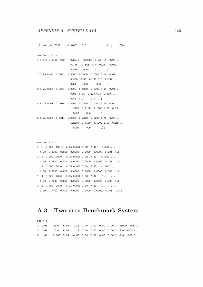
APPENDIX A. SYSTEM DATA 146
13 14 0.17093 0.34802 0.0 1. 0.]; %20
mac_con = [ ...
1 1 615 0.1725 0.0 0.8979 0.2995 0.23 7.4 0.03 ...
0.746 0.646 0.4 0.25 0.033 ...
5.548 0.00 0.0 ;
2 2 75 0.00 0.0031 1.0500 0.1850 0.1300 6.10 0.04...
0.980 0.36 0.130 0.3 0.099...
6.54 0.0 0.0 ;
3 3 75 0.00 0.0031 1.0500 0.1850 0.1300 6.10 0.04...
0.98 0.36 0.130 0.3 0.099 ...
6.54 0.0 0.0 ;
4 6 25 0.09 0.0014 1.2500 0.2320 0.1200 4.75 0.06 ...
1.2200 0.7150 0.1200 1.50 0.21 ...
5.06 0.0 0 ;
5 8 25 0.09 0.0014 1.2500 0.2320 0.1200 4.75 0.06...
1.2200 0.7150 0.1200 1.50 0.21...
5.06 0.0 0];
exc_con = [...
1 1 0.000 190.0 0.05 0.000 0.00 7.32 -1.000 ...
1.00 0.1900 0.000 0.0000 0.0000 0.0000 0.001 1.0;
1 2 0.000 20.0 0.05 0.000 0.00 7.32 -1.000 ...
1.00 1.9800 0.000 0.0000 0.0000 0.0000 0.005 1.0;
1 3 0.000 20.0 0.05 0.000 0.00 7.32 -1.000 ...
1.00 1.9800 0.000 0.0000 0.0000 0.0000 0.005 1.0;
1 4 0.000 20.0 0.05 0.000 0.00 7.32 -1. ...
1.00 0.7000 0.000 0.0000 0.0000 0.0000 0.005 1.0;
1 5 0.000 20.0 0.05 0.000 0.00 7.32 -1. ...
1.00 0.7000 0.000 0.0000 0.0000 0.0000 0.005 1.0];
A.3 Two-area Benchmark System
bus = [
1 1.03 26.0 6.84 1.31 0.00 0.00 0.00 0.00 1 990.0 -990.0;
2 1.01 17.0 5.00 1.13 0.00 0.00 0.00 0.00 2 5.0 -300.0;
3 1.03 0.045 9.24 0.67 0.00 0.00 0.00 0.00 2 5.0 -300.0;

APPENDIX A. SYSTEM DATA 147
4 1.01 -1.97 7.00 0.43 0.00 0.00 0.00 0.00 2 5.0 -300.0;
5 1.01 20. 0.00 0.00 0.00 0.00 0.00 0.00 3 0.0 0.0;
6 0.98 10.8 0.00 0.00 0.00 0.00 0.00 0.00 3 0.0 0.0;
7 0.97 4.79 0.00 0.00 9.67 1.00 0.00 2.00 3 0.0 0.0;
8 0.9503 0.49 0.00 0.00 0.00 0.00 0.00 0.00 3 0.0 0.0;
9 0.97 -13.14 0.00 0.00 17.67 1.00 0.00 3.50 3 0.0 0.0;
10 0.9862 -8.54 0.00 0.00 0.00 0.00 0.00 0.00 3 0.0 0.0;
11 1.01 -6.52 0.00 0.00 0.00 0.00 0.00 0.00 3 0.0 0.0];
line = [...
1 5 0.0 0.0167 0.00 1.0 0.;
2 6 0.0 0.0167 0.00 1.0 0.;
3 11 0.0 0.0167 0.0 1.0 0.;
4 10 0.0 0.0167 0.0 1.0 0.;
5 6 0.0025 0.025 0.04375 1.0 0.;
6 7 0.001 0.0100 0.0175 1.0 0.;
6 7 0.002 0.0200 0.0170 1.0 0.;
10 9 0.00125 0.0100 0.0175 1.0 0.;
9 10 0.005 0.0125 0.0035 1.0 0.;
7 8 0.0075 0.005 0.12833 1.0 0.;
7 8 0.0075 0.075 0.12833 1.0 0.;
7 8 0.0075 0.075 0.12833 1.0 0.;
7 8 0.0075 0.075 0.12833 1.0 0.;
8 9 0.018 0.180 0.1925 1.0 0.;
8 9 0.018 0.180 0.1925 1.0 0.;
8 9 0.018 0.180 0.1900 1.0 0.;
11 10 0.0025 0.005 0.0140 1.0 0.
];
mac_con = [...
1 1 900 0.200 0.0025 1.8 0.30 0.25 8.00 0.03...
1.7 0.55 0.25 0.4 0.05...
6.5 0 0 1;
2 2 900 0.200 0.0025 1.8 0.30 0.25 8.00 0.03...
1.7 0.55 0.25 0.4 0.05...
6.5 0 0 2;
3 3 900 0.200 0.0025 1.8 0.30 0.25 8.00 0.03...
1.7 0.55 0.25 0.4 0.05...
5.175 0 0 3;
4 4 900 0.200 0.0025 1.8 0.30 0.25 8.00 0.03...

APPENDIX A. SYSTEM DATA 148
1.7 0.55 0.25 0.4 0.05...
6.175 0 0 4];
exc_con = [...
0 1 0.0 100 0.02 0.0 0.0 7 -7 ...
0 0 0 0 0 0 0 0 0 0 0 ;
0 2 0.0 100 0.02 0.0 0.0 7 -7 ...
0 0 0 0 0 0 0 0 0 0 0 ;
0 3 0.0 75 0.02 0.0 0.0 7 -7 ...
0 0 0 0 0 0 0 0 0 0 0 ;
0 4 0.0 50 0.02 0.0 0.0 7 -7 ...
0 0 0 0 0 0 0 0 0 0 0 ;
];
tg_con = [
1 1 1 5 25 5 0.01 0.01 0.01 0.01;
];
%Power System Stabilizer (PSS)
%Column
%1 type
%1 speed input
%2 power input
%2 machine number
%3 gain K
%4 washout time constant T sec
%5 lead time constant T1 sec
%6 lag time constant T2 sec
%7 lead time constant T3 sec
%8 lag time constant T4 sec
%9 maximum output limit pu
%10 minimum output limit pu
pss_con = [...
1 1 6.0 2.0 0.08 0.04 0.08 0.04 10 -10;
1 2 6.0 2.0 0.08 0.04 0.08 0.04 10 -10;
1 3 6.0 2.0 0.08 0.04 0.08 0.04 10 -10;
1 4 6.0 2.0 0.08 0.04 0.08 0.04 10 -10
];
Appendix B
SISI Proof
From equation (4.4), the singular values of the matrix Λm are defined as:
svi(Λm) =√
µi (Q) for i = 1, 2, · · · , 2n (B.1)
Q = Λ∗m Λm ∈ ℜ2n×2n (B.2)
where µi(Q) denotes the ith eigenvalue of Q, and Λ∗m is the transpose conjugate of
Λm. Thus,
Q = Λ∗m Λm =
Λ∗Λ + β2
c I βc(Λ − Λ∗)
βc(Λ∗ − Λ) Λ∗Λ + β2
c I
(B.3)
Then, these submatrices can be expressed in terms of the eigenvalues in Λ (λi =
αi ± jβi) as:
Λ∗Λ + βcI = diag|λ1|2 + β2c , |λ2|2 + β2
c , · · · , |λn|2 + β2c ∈ ℜn×n (B.4)
βc(Λ − Λ∗) = (2j βc) diagβ1, β2, · · · , βn ∈ ℜn×n (B.5)
Thus, the characteristic equation of Q can be obtained as:
∆(s) = det(sI − Q) = [(s − |λ1|2 − β2c )
2 − (2β1βc)2] [(s − |λ2|2 − β2
c )2 − (2β2βc)
2]
· · · [(s − |λn|n − β2c )
2 − (2βnβc)2] (B.6)
149

APPENDIX B. SISI PROOF 150
The roots of the characteristic equation are the eigenvalues of Q, which can be
written as
µi(Q) = α2i + (βc ± βi)
2 (B.7)
Thus, (B.7) and (B.1) yields (4.5). ⋄

Appendix C
Alternative Damping Torque
Formulation
In order to calculate Dj in (5.5), it is possible to separate the states as ∆x =
[∆ωj ∆xd]T , and hence rewrite the linearized state-space model as follows:
∆xd = Ax ∆xd + Bω ∆ωj (C.1)
∆ωj = Aω ∆ωj + Bx ∆xd (C.2)
∆Tej= Cd ∆xd + Cωj
∆ωj (C.3)
Replacing d/dt by s in (C.1) would yield ∆xd = (sI − Ax)−1Bω∆ωj. Thus:
Dj(s) =∆Tej
∆ωj
=(Cd (s I − Ax)
−1 Bω + Cωj
)(C.4)
Evaluating Dj(s = λi) would give the same results as (5.5). In [6], the author pro-
poses a method to obtain transfer functions similar to (C.4) by disabling the shaft
dynamics in all machines, resulting in various transfer functions. These functions
are used to show the inherent damping and interaction between different machines.
151

APPENDIX C. ALTERNATIVE DAMPING TORQUE FORMULATION 152
However, the procedure shown here is equivalent to disabling only the shaft dy-
namics for machine j; this means that (C.4) includes the induced damping and
synchronizing torques of all machines on the shaft of Machine j.
Bibliography
[1] E. Uzunovic, “Transient Stability and Power Flow Models of VSC FACTS con-
trollers,” Ph.D. dissertation, University of Waterloo, Waterloo, ON, Canada,
2001.
[2] “Interim Report: Causes of the August 14th Blackout in the United States
and Canada,” Tech. Rep., November 2003, available at http://www.nrcan-
rncan.gc.ca/media/docs/814BlackoutReport.pdf.
[3] “Report on the events of September 28th, 2003 culminating in the separation
of the Italian power system from the other UCTE networks,” Tech. Rep., April
2004, available at http://www.autorita.energia.it/docs/04/061-04all.pdf.
[4] “The black-out in southern Sweden and eastern Denmark,
23 September, 2003,” Tech. Rep., October 2003, available at
http://www.svk.se/upload/3195/Disturbance Sweden DenmarkSept23.pdf.
[5] “System Disturbance Stability Studies for Western System Coordinating Coun-
cil (WSCC),” EPRI Final Report prepared by Powertech Labs Inc., Surrey,
BC, Canada, Tech. Rep. TR-108256, September 1997.
153

BIBLIOGRAPHY 154
[6] M. J. Gibbard, “Co-ordinated design of multimachine power system stabilisers
based on damping torque concepts,” IEE Proceedings, Pt. C, vol. 135, no. 4,
pp. 276–284, July 1988.
[7] C. A. Canizares, editor, “Voltage Stability Assessment: Concepts, Practices
and Tools,” Special Publication of IEEE Power System Stability Subcommit-
tee, Tech. Rep. SP101PSS, August 2002.
[8] N. Mithulananthan, “Hopf bifurcation control and indices for power system
with interacting generator and FACTS controllers,” Ph.D. dissertation, Uni-
versity of Waterloo, Waterloo, ON, Canada, 2002.
[9] C. A. Canizares, N. Mithulananthan, A. Berizzi, and J. Reeve, “On the linear
profile of indices for the prediction of saddle-node and limit-induced bifurcation
points in power systems,” IEEE Trans. Circuits and Systems, vol. 50, no. 2,
pp. 1588–1595, December 2003.
[10] C. A. Canizares, A. C. Z. de Souza, and V. Quintana, “Comparison of per-
formance indices for detection of proximity to voltage collapse,” IEEE Trans.
Power Systems, vol. 11, no. 3, pp. 1441–1450, August 1996.
[11] V. Ajjarapu and B. Lee, “Bifurcation theory and its application to nonlinear
dynamical phenomena in an electrical power system,” IEEE Trans. Power
Systems, vol. 7, no. 1, pp. 424–431, 1992.
[12] W. Zhu, R. Mohler, R. Spee, W. A. Mittelstadt, and D. Maratukulam, “Hopf
bifurcation in a SMIB power system with SSR,” IEEE Trans. Power Systems,
vol. 11, no. 7, pp. 1579–1584, 1996.

BIBLIOGRAPHY 155
[13] C. A. Canizares, N. Mithulananthan, F. Milano, and J. Reeve, “Linear per-
formance indices to predict oscillatory stability problems in power systems,”
IEEE Trans. Power Systems, vol. 19, no. 2, pp. 1104–1114, May 2004.
[14] T. Kim and E. H. Abed, “Closed-loop monitoring system for detecting im-
pending instability,” IEEE Trans. Circuits and Systems, vol. 47, no. 10, pp.
1479–1493, October 2000.
[15] N. Mithulananthan, C. A. Canizares, J. Reeve, and G. J. Rogers, “Comparison
of PSS, SVC and STATCOM controllers for damping power system oscilla-
tions,” IEEE Trans. Power Systems, vol. 18, no. 2, pp. 786–792, May 2003.
[16] “Power Dynamics Management (PDM),” Psymetrix Limited, Scotland, UK,
Tech. Rep., available at www.psymetrix.com.
[17] D. H. Wilson, “Managing oscillatory stability using on-line dynamics mea-
surements,” in Power System Conference & Exposition, New York, October
2004.
[18] I. Fernando, L. Chung, L. Midford, A. Silk, R. Coish, A. Golder, K. Hay,
and D. Wilson, “Real time online evaluation of small signal system damping
applied to power system stabilizer commissioning and testing,” in International
Conference on Power Systems Transients - IPST, New Orleans, 2003.
[19] J. F. Hauer, “The use of Prony analysis to determine modal content and equiv-
alent models for measured power system response,” in IEEE/PES Symposium
on Application of Eigenanalysis and Frequency Domain Methods for System
Dynamic Performance, July 1989, pp. 105–115.

BIBLIOGRAPHY 156
[20] J. R. Smith, F. Fatehi, C. S. Woods, J. F. Hauer, and D. J. Trudnowski,
“Transfer function identification in power system applications,” IEEE Trans.
Power Systems, vol. 8, no. 3, pp. 1282–1290, August 1993.
[21] J. F. Hauer, “Application of Prony analysis to the determination of modal
content and equivalent models for measured power system response,” IEEE
Trans. Power Systems, vol. 6, no. 3, pp. 1062–1068, August 1991.
[22] B. J. Bujanowski, J. W. Pierre, S. M. Hietpas, T. L. Sharp, and D. A. Pierre, “A
comparison of several system identification methods with application to power
systems,” in IEEE Proceedings of the 36th Midwest Symposium on Circuits
and Systems, vol. 1, August 1993, pp. 64–67.
[23] R. W. Wies, J. W. Pierre, and D. J. Trudnowski, “Use of ARMA block process-
ing for estimating stationary low-frequency electromechanical modes of power
systems,” IEEE Trans. Power Systems, vol. 18, no. 1, pp. 167–173, 2003.
[24] J. W. Peirre, D. J. Trudnowski, and M. Donnelly, “Initial results in electrome-
chanical mode identification from ambient data,” IEEE Trans. Power Systems,
vol. 12, no. 3, pp. 1245–1251, August 1997.
[25] M. K. Pal, “Voltage stability conditions considering load characteristics,” IEEE
Trans. Power Systems, vol. 7, pp. 243–247, February 1992.
[26] W. S. Kao, “The effect of load models on unstable low-frequency oscillation
damping in taipower system experience w/wo power system stabilizers,” IEEE
Trans. Power Systems, vol. 16, pp. 463–472, August 2001.
[27] C. A. Canizares, “On bifurcations, voltage collapse and load modeling,” IEEE
Trans. Power Systems, vol. 10, pp. 512–522, February 1995.

BIBLIOGRAPHY 157
[28] M. H. J. Bollen, G. Yalcinkaya, and G. Hazza, “The use of electromagnetic
transient program for voltage sag analysis,” in Proc. 8th International Confer-
ence on Harmonics And Quality of Power, vol. 1, October 1998, pp. 598–603.
[29] G. Rogers, Power Sysem Oscillations. Boston/London/Dordrecht: Kluwer
Academic Publishers, 2000.
[30] M. Klein, G. J. Rogers, and P. Kundur, “A fundamental study of inter-area
oscillation in power systems,” IEEE Trans. Power Systems, vol. 6, no. 3, pp.
914–921, 1991.
[31] N. Mithulananthan, C. A. Canizares, and J. Reeve, “Hopf bifurcation control
in power system using power system stabilizers and static var compensators,”
in Proc. of NAPS’99, San Luis Obispo, California, October 1999, pp. 155–163.
[32] Y. Ni and L. Snider, “STATCOM power frequency model with VSC charging
dynamics and its application in power system stability analysis,” in Proceedings
of APSCOM’97, Hong Kong, November 1997, pp. 119–125.
[33] P. Kundur, Power System Stability and Control. New York: McGraw-Hill,
1994.
[34] F. Milano, Power System Analysis Toolbox (PSAT), Version 1.3.4, User Man-
ual, 2005, available at http://www.power.uwaterloo.ca/∼fmilano.
[35] F. P. Demello and C. Concordia, “Concepts of synchronous machine stability
as affected by excitation control,” IEEE Trans. Power Apparatus and Systems,
vol. PAS-88, no. 4, pp. 316 – 329, April 1969.
[36] Power System Toolbox (PST) Version 2.0: Dynamics Tutorial and Functions,
Cherry Tree Scientific Software, 2002.

BIBLIOGRAPHY 158
[37] G. Hingrani, Understanding FACTS. New York: IEEE Press, 2000.
[38] A. E. Hammad, “Comparing the voltage control capabilities of present and
future var compensating techniques in transmission systems,” IEEE Trans.
Power Delivery, vol. 11, no. 1, pp. 475–484, January 1996.
[39] E. Larsen, S. Nilsson, N. Miller, and S. Lindgren, “Benefits of gto-based com-
pensation systems for electric utility applications,” IEEE Trans. Power Deliv-
ery, vol. 7, no. 4, pp. 2056–2062, October 1992.
[40] C. A. Canizares, M. Pozzi, and E. Uzunovic, “STATCOM modeling for volt-
age and angle stability studies,” International Journal of Electrical Power &
Energy Systems, vol. 25, no. 6, pp. 431–441, June 2003.
[41] V. Venkatasubramanian, H. Schattler, and J. Zaborsky, “Dynamics of large
constrained nonlinear systems-a taxonomy theory [power system stability],” in
Proceedings of the IEEE, vol. 83, no. 11, November 1995, pp. 1530–1561.
[42] N. Mithulananthan and S. C. Sirvastava, “Investigation of a voltage collapse
incident in Sri Lanka’s power system network,” in EMPD’98, Singapore, March
1998, pp. 47–52.
[43] C. A. Caizares and F. L. Alvarado, “Point of collapse and continuation methods
for large ac/dc systems,” IEEE Trans. Power Systems, vol. 8, no. 1, pp. 1–8,
February 1993.
[44] Transient Security Assessment Tool (TSAT), User Manual, Powertech Labs
Inc., Surrey, BC, Canada, V3W 7R7, 2002.
[45] System Identification Toolbox Version 5.0.1. www.Mathworks.com, 18-May-
2001.

BIBLIOGRAPHY 159
[46] S. K. M. Kodsi and C. A. Canizares, “Modeling and simulation of IEEE 14-bus
system with FACTS controllers,” University of Waterloo, Canada, Tech. Rep.,
March 2003, available at www.power.uwaterloo.ca.
[47] Power Flow and Short-circuit Analysis Tool (PSAT), Version 5.1, User Man-
ual, Powertech Labs Inc., Surrey, BC, Canada, V3W 7R7, 2002.
[48] Voltage Security Assessment Tool (VSAT), Version 5.2, User Manual, Pow-
ertech Labs Inc., Surrey, BC, Canada, V3W 7R7, 2002.
[49] Small Signal Analysis Tool (SSAT), User Manual, Powertech Labs Inc., Surrey,
BC, Canada, V3W 7R7, 2002.
[50] S. L. Marple, Digital Spectral Analysis. Englewood Cliffs, N.J.: Prentice Hall,
1987.
[51] Y. Hua and T. K. Sarkar, “Generalized pencil-of-function method for extract-
ing poles of an EM system from its transient response,” IEEE Trans. Antenna
and Propagation, vol. 37, no. 2, pp. 229–234, February 1989.
[52] J. F. Hauer, C. J. Demeure, and L. L. Scharf, “Initial results in Prony analysis
of power system response signals,” IEEE Trans. Power Systems, vol. 5, no. 1,
pp. 80–89, February 1990.
[53] D. J. Trudnowski, J. M. Johnson, and J. F. Hauer, “Making Prony analysis
more accurate using multiple signals,” IEEE Trans. Power Systems, vol. 14,
no. 1, pp. 226–231, February 1998.
[54] D. J. Trudnowski, J. R. Smith, T. A. Short, and D. A. Pierre, “An application
of Prony methods in PSS design for multimachine systems,” IEEE Trans.
Power Systems, vol. 6, no. 1, pp. 118–126, February 1991.

BIBLIOGRAPHY 160
[55] D. W. Tufts and R. Kumaresan, “Singular value decompsition and improved
frequency estimation using linear prediction,” IEEE Trans. Acoustics, Speech,
and Signal Processing, vol. ASSP-30, no. 4, pp. 671–675, August 1982.
[56] S. M. Kay, Modern Spectral Estimation: Theory and Application. Englewood
Cliffs, N.J.: Prentice Hall, 1988.
[57] M. L. VanBlaricum and R. Mittra, “Problems and solutions associated with
prony’s method for processing transient data,” IEEE Trans. Antennas and
Propagation, vol. AP-26, no. 1, pp. 174–182, January 1978.
[58] L. Ljung, System Identification: Theory for the User, 2nd ed. Englewood
Cliffs, N.J.: Prentice-Hall, 1999.
[59] R. Soderstrom, System Identification. Cambridge, UK: Prentice Hall Inter-
national (UK) Ltd., 1989.
[60] B. Friedlander, “Instrumental variable methods for ARMA spectral estima-
tion,” IEEE Trans. Acoustics, Speech, and Signal Processing, vol. ASSP-31,
no. 2, pp. 404–415, April 1983.
[61] P. V. Overshee and B. D. Moor, Subspace Identification for Linear Systems:
Theory-Implementation-Applications. Kluwer Academic Publishers, 1996.
[62] D. Bauer, “Subspace Algorithms,” 2003, seminar notes, available at
http://cowles.econ.yale.edu/seminars/ecm03/bauer-031022.pdf.
[63] B. Dietmar, “Asymptotic efficiency of CCA subspace methods in the case of
no exogenous inputs,” Department of Electrical and Computer Engineering,
Linkoping University, SE-581 83, Linkoping, Sweden, Tech. Rep. LiTH-ISY-
R-2262, 2000.

BIBLIOGRAPHY 161
[64] R. T. H. Alden and A. A. Shaltout, “Analysis of damping and synchronous
torques: Part I - A general calculation method,” IEEE Trans. Power Systems,
vol. PAS-98, no. 5, pp. 1696–1700, Sept/Oct 1979.
[65] A. A. Shaltout and B. A. Abu Al-Feilat, “Damping and synchronous torque
computation in multimachine power systems,” IEEE Trans. Power Systems,
vol. 7, no. 1, pp. 280–286, February 1992.
[66] P. Pourbeik and M. J. Gibbard, “Damping and synchronizing torques in-
duced on generators by facts stabilizers in multimachine power systems,” IEEE
Trans. Power Systems, vol. 11, no. 4, pp. 1920–1925, November 1996.
[67] T. C. Hsia, System Identification: Least-Square Methods. Lexington, MA:
Lexington Books, D.C. Health and Company, 1977.
[68] Statistic Toolbox 1.1 in MATLAB, The Mathworks, 2000.
[69] A. Pankratz, Forecasting with Univariate Box-Jenkins Models: Concepts and
Cases, 1st ed. New York: Wiley, 1983.
[70] P. Andersen, “Identification of civil engineering structures using vector ARMA
models,” Ph.D. dissertation, Aalborg University, Aalborg, Denmark, 1997.
[71] L. Ljung, System Identification Theory for the User. Englewood Cliffs, N.J.:
Prentice Hall, 1999.
[72] On the Use of Power System Computer Aided Design (PSCAD) Version 4.0.3,
User’s Guide, Manitoba HVDC Research Centre, 244 Cree Crescent, Win-
nipeg, Manitoba, Canada R3J 3W1, 2003.

BIBLIOGRAPHY 162
[73] T. J. Hammons et al., “Effect of damper modelling and the fault clearing
process on response torque and stressing of turbine generator rotors,” IEEE
Trans. Energy Conversion, vol. EC-1, no. 9, p. 113, 1986.
[74] T. Kumano et al., “Effect of back swing phenomena upon transient stability,”
Trans. IEE of Japan, vol. 109-B, no. 9, p. 403, 1989.
[75] I. D. Landau, System Identification and Control Design. Englewood Cliffs,
N.J.: Prentice Hall, 1990.
[76] Small Signal Stability Program (SSSP) Version 3.1, User’s Manual, Ontario
Hydro, 1994.
[77] N. Mohan, T. M. Undeland, and W. P. Robbins, Power Electronics : Convert-
ers, Applications, and Design, 2nd ed. NJ: Wiley, 1994.
[78] H. Ghasemi, C. A. Canizares, and A. Moshred, “Oscillatory stability limit pre-
diction using stochastic subspace identification,” IEEE Trans. Power Systems,
vol. 21, no. 2, pp. 736–745, May 2006.
[79] H. Ghasemi, C. A. Canizares, and J. Reeve, “Prediction of instability points
using system identification,” in Proc. Bulk Power System Dynamics and Con-
trol - VI, Cortina D′Ampezzo, Italy, August 2004, 6 pages.
[80] H. Ghasemi and C. A. Canizares, “Damping torque estimation and oscillatory
stability margin prediction,” accepted to IEEE Power Engineering Summer
Meeting, Montreal, Canada, June 2006, 6 pages.