On-line Support Vector Regression of the Transition

Model for the Kalman Filter

Samuele Saltia, Luigi Di Stefanoa

aViale Risorgimento, 2 - 40135 Bologna, Italy

Abstract

Recursive Bayesian Estimation (RBE) is a widespread solution for visual

tracking as well as for applications in other domains where a hidden state is

estimated recursively from noisy measurements. From a practical point of

view, deployment of RBE filters is limited by the assumption of complete

knowledge on the process and measurement statistics. These missing to-

kens of information lead to an approximate or even uninformed assignment

of filter parameters. Unfortunately, the use of the wrong transition or mea-

surement model may lead to large estimation errors or to divergence, even

when the otherwise optimal filter is deployed. In this paper on-line learning

of the transition model via Support Vector Regression is proposed. The

specialization of this general framework for linear/Gaussian filters, which

we dub Support Vector Kalman (SVK), is then introduced and shown to

outperform a standard, non adaptive Kalman filter as well as a widespread

solution to cope with unknown transition models such as the Interacting

Multiple Models (IMM) filter.

Keywords: Adaptive Transition Model, Visual Tracking, Support Vector

Regression, Kalman filter, Interacting Multiple Models

Email addresses: samuele.salti@unibo.it (Samuele Salti),Preprint submitted to Image and Vision Computing April 18, 2013

The problem of hidden state estimation from noisy measurements is

transversal to several disciplines, such as Statistic, Control Theory, Econo-

metrics and, last but not least, Computer Vision. In Computer Vision, this

problem usually emerges in the Filtering and Data Association [1] compo-

nent of visual tracking algorithms, and it is typically dealt with by Recursive

Bayesian Estimation (RBE) [2].

One of the main drawbacks to the deployment of this powerful and

sound framework consists in the requirement to a priori specify a process

dynamic, i.e. a transition model between states, that the user believes the

system obeys. In many cases, this model is unknown and hence, empirically

selected among a restricted set of standard ones. This approximate tuning

of a recursive Bayesian filter may seriously degrade its performance, that

could be optimal in case of correct system identification. Another solution

to cope with the lack of knowledge on the transition model is to treat the

system as a jump Markov system, i.e. a system that can follow different

models at different time steps. Under this assumption, the user provides

the RBE filter with a pool of possible models and let it choose the most

likely one in each time frame, thereby having the filter partially tackling the

uncertainty on the real system dynamics. Nevertheless, the choice of the

models in the pool is left to the user and therefore, prone to error.

In this work we take a novel perspective to transition model identifica-

tion: we propose to learn the transition model on-line by feeding the filter

evolution to Support Vector Machines in regression mode (SVR). We pro-

vide first a conceptual solution suited to the general formulation of RBE

and we discuss some issues related to every specific instantiation of this

luigi.distefano@unibo.it (Luigi Di Stefano)2

general model. Then, we address the Gaussian/linear case and provide a

detailed solution for the Kalman Filter, dubbed Support Vector Kalman

(SVK) filter. Our choice is motivated by the state-of-the-art performance

demonstrated by SVR [3] as well as, in case of Gaussian/linear systems,

by the sound theoretical match between the assumptions on uncertainties

underlying Kalman filtering and SVR. The SVK filter drastically reduces

the number of parameters to be specified by the user, in particular the pro-

cess noise covariance matrix, which is typically hard to estimate, but plays

a significant role with respect to filter performance. Our algorithm also

allows for obtaining a time-variant estimation of the transition model, and

therefore results in a more adaptive filter than those usually proposed in

previous literature. A preliminary version of our work was presented in [4].

1. Recursive Bayesian Estimation

The problem of hidden state estimation, xk ∈ Rn, from noisy measures,

zk ∈ Rm, is typically solved in discrete-time systems via Recursive Bayesian

Estimation. In this framework the system is completely specified by a first

order Markov model compound of a law of evolution of the state, a mea-

surement process and an initial state x0.

In a Bayesian approach, given the uncertainty affecting both the law of

evolution of the state as well as the measurement process, represented by

the noise Random Variables νk ∈ Rn and ηk ∈ Rm affecting, respectively,

the state evolution and the measurement process, the entities comprising

the system are defined by PDFs, i.e. following the notation in [2],

• the transition model xk = fk(xk−1, νk) is modeled by the PDF p(xk | xk−1);

3

• the observation likelihood zk = hk(xk, ηk) is modeled by the PDF

p(zk | xk);

• the initial state is known via its PDF p(x0).

These PDFs are generally assumed to be known a priori and never updated.

Given this characterization of the target motion, a general but concep-

tual solution to the tracking problem can be obtained in two steps: pre-

diction and update [2] (Fig. 2). In the prediction stage, the Chapman-

Kolmogorov equation is used to propagate the belief on the state at time

k − 1 to time k

p(xk | z1:k−1) =

∫p(xk | xk−1)p(xk−1 | z1:k−1) dxk−1. (1)

where z1:k−1 is the set of all measurements up to frame k−1, {z1, . . . , zk−1}.

This usually corresponds to a spreading of the belief on the state, due to

the increasing distance in time from the last measurement. In the update

stage, the PDF is sharpened again by using the current measure zk and the

Bayes rule

p(xk | z1:k) ∝ p(zk | xk)p(xk | z1:k−1). (2)

This conceptual solution is analytically solvable only in a few cases. A

notable one is when the law of evolution of the state and the measurement

equations are linear and noises are Gaussian. In this situation, the optimal

solution is provided by the Kalman filter [5]. The RBE framework for this

case becomes:

xk = fk(xk−1, νk) ⇒ xk = Fkxk−1 + νk, E[νkν

Tk

]= Qk (3)

zk = hk(xk, ηk) ⇒ zk = Hkxk + ηk, E[ηkη

Tk

]= Rk. (4)

4

12.5

13

13.5

14

14.5

15

15.5

16

16.5

0 50 100 150 200 250 300

Erro

r

Time

Vel

0

2000

4000

6000

8000

10000

12000

0 50 100 150 200 250 300

Erro

r

Time

Vel

(a) (b)

Figure 1: The impact of a wrong transition model: (a) the Kalman estima-

tion exhibits, apart from the noise effect, a constant error (actual velocity

- estimated velocity) if the wrong transition model is used; (b) the Kalman

estimation diverges from the true velocity (i.e. the error increases) if a per-

turbed transition model is used (the noise effect is hardly perceivable here

because of the much larger error scale).

and the mean and covariance matrix of the Gaussian posterior can be op-

timally estimated using the Kalman filter equations [5]. We will refer to

Fk ∈ Rn×n and Qk ∈ Rn×n as the transition matrix and the transition

covariance, respectively.

2. Motivation

The difficulty of identifying a proper transition model for a specific ap-

plication typically leads to empirical and suboptimal tuning of the filter

parameters. The most widespread solutions to specify a transition model

for tracking are to empirically select it among a restricted set of standard

ones (such as constant position, i.e. Brownian motion, [6–8] or constant

velocity [1, 9–11]) or learn it off-line from representative training data [12].5

Besides the availability of these training sequences, which depends on the

particular application, the major shortcoming of these solutions is that they

do not allow to change the transition model through time, although this can

be beneficial and neither the conceptual solution nor the solving algorithms

require it to be fixed.

Approximate tuning of a recursive Bayesian filter may seriously degrade

its performances, that could be optimal (e.g., when the assumptions of

Kalman filtering are met) in case of correct system identification. In Fig.

1 we present two simple experiments to highlight the strong, detrimental

impact of a wrongly identified transition model on an otherwise optimal

and correctly tuned recursive Bayesian filter. In these simulations a point

is moving along a line with constant acceleration and we try to estimate its

position and velocity by two Kalman filters from measurements corrupted

with Gaussian noise, whose constant covariance matrix is known and used

as the measurement noise covariance matrix of the filters, Rk. Hence, we

are using the optimal estimator given the experimental setup. The only

parameter that is wrongly tuned is the transition model, in particular, in

one simulation we use a constant velocity transition matrix Fk instead of a

constant acceleration one, whereas in the second simulation the transition

model is a constant acceleration matrix whose parameters are perturbed by

5% of their value. The transition covariance matrix, Qk, was set very high,

in order to compensate for the wrong transition matrix. Despite this, when

using the wrong transition model the estimation exhibits a constant bias

with respect to the real value while, when using the perturbed transition

model the estimated and the true value of the velocity diverge. In other

words, the estimation of an otherwise optimal estimator like the Kalman fil-

6

ter can be arbitrarily wrong when an incorrect transition model is assumed.

This highlights the main motivation behind our work.

3. Related work

Closely related to our work are the efforts devoted to the derivation of

adaptive Kalman filters, that have been studied since the introduction of

this filtering technique. In fact, our proposal can be seen as a new approach

to build an adaptive Kalman filter. The main idea behind adaptive filter-

ing schemes is that the basic source of uncertainty is due to the unknown

noise covariances, and the proposed solution consists in estimating them

on-line from observed data. One of the most comprehensive contributions

in this field is provided in [13]. The paper reviews proposed approaches

and classifies them according to four categories: Bayesian Estimation (BE),

Maximum Likelihood Estimation (MLE), Correlation Methods (CM) and

Covariance-Matching Techniques (CMT). Methods in the first category im-

ply integration over a large dimensional space and can be solved only with

special assumptions on the PDF of the noise parameters. MLE requires the

solution of a non-linear equation that, in turns, is solvable only under the as-

sumptions that the system is time invariant and completely observable and

the filter has reached a steady state. Under these assumptions, however,

only a time invariant estimation of the parameters of the noise PDF can be

obtained. Correlation Methods, too, are applicable only to time invariant

and completely observable systems. Finally, Covariance-Matching Tech-

niques can estimate either process or measurement noise parameters and

turn out to provide good and time-varying approximations for the measure-

ment noise when the process noise is known.7

In [14], an improved correlation method is proposed, but the require-

ment on the stationarity of the system is not dropped. In [15], an approach

able to simultaneously estimate both transition and covariance matrices,

even if they are time-varying, is proposed. It is based on the construction

of a recursive sequence of positive definite matrices representing the up-

per bounds for the real covariance matrices. Covariance matrices are then

determined by minimizing such bounds, which turns out to require a time-

consuming convex optimization problem. In the context of visual tracking,

[16] presents the application of an adaptive Kalman filter. The process and

measurement errors are modified at every frame taking into account the

degree of occlusion of the target: greater occlusion corresponding to greater

value of measurement noise and vice versa, the two noises always summing

up to one. In the extreme case of total occlusion, measurement noise is

set to infinity and process noise to 0. The method in [17] uses the term

Adaptive to refer to an adaptive forgetting factor, that is used to trade off

the contribution to the covariance estimate at the current time step of the

covariance estimates for the previous time step and process noise. This is

done to improve responsiveness of the filter in case of abrupt state changes.

Compared to all these proposals, our method makes no assumptions on

the system. This allows our method to be more widely applicable and, in

particular, to fit better the usual working conditions visual trackers have

to deal with. Moreover, unlike BE, MLE and CM techniques, our proposal

provides a time-varying noise statistics estimation. This is extremely im-

portant to allow the filter to dynamically weight the prediction on the state

and the noisy measurement it has to fuse at each frame, e.g. to cope with

occlusions when the measurement can be totally wrong and the prediction

8

on the state is the only reliable source of information to keep on tracking

the target. Unlike [16], our proposal is not specifically conceived for visual

tracking and, hence, generally applicable. On the other hand, a general

proposal like the one in [15], turns out to be less attractive for visual track-

ing than our filter, given the higher computational requirements. Finally,

it is worth pointing out that, unlike all reviewed approaches, our proposal

is adaptive in a broader sense, for it identifies on-line not only the process

noise covariance matrix but also the transition matrix.

Another approach to deal with unknown covariance matrices and tran-

sition models is to rely on multiple standard models and let the filter choose

the most adequate one in each time frame, that is effectively modeling it as

Jump Markov system [2]. A celebrated algorithm based on this idea is the

Interacting Multiple Model (IMM) filter [18], that has been used also for

visual tracking [19, 20]. We will show in the experimental results how our

approach consistently outperforms IMM, having also the additional advan-

tage to expose the user to less free parameters to be specified.

4. SVMs in ε-regression mode

Our approach to transition model identification is based on Support

Vector Machines [21] in ε-regression mode (SVR) [3]. To make the paper

self-contained, we provide a brief description of them.

To introduce SVMs as regressors, and in particular in ε-regression mode,

let us have a quick look at the regression of a linear model given a series of

data (xi, yi). In ε-regression mode the SVR tries to estimate a function of x

that is far from training data yi at most ε and is at the same time as flat as

possible. The requirement of flatness comes from the theory of complexity9

developed by [21] and ensures that we will get a solution with minimal

complexity (hence, with better generalization abilities). In the linear case,

the model we fit on the data is

f (x) = 〈w,x〉+ b (5)

and the solution with minimal complexity is given by the unique solution

of the following convex optimization problem

min12||w| |2 + C

∑li=1(ξi + ξ∗i )

yi − 〈w,xi〉 − b ≤ ε+ ξi

yi − 〈w,xi〉 − b ≥ −ε− ξ∗i

(6)

The constant C is a parameter and weights the deviations from the model

greater than ε. The problem is then usually solved using its dual form,

that is easier both to solve and to extend so as to estimate also non-linear

functions ([21]).

5. On-line transition model adaptation

We propose to overcome the difficulties and shortcomings due to empir-

ical tuning of the transition model by adapting it on-line.

In other terms, we propose to avoid to define p(xk|xk−1), and instead

use in its place a learned PDF p̃(xk|xk−1), derived from a learned f̃k.

Furthermore, we propose to learn the motion model using SVRs. A first

reason to employ SVMs lays in their solid theoretical foundations, based

on the statistical learning theory developed by Vapnik and Chervonenkis,

which guarantee their ability to generalize from training data minimizing

10

the over-fitting problem. Their use as regressors is probably less popu-

lar but even in this field they provide excellent performances [3]. In the

case of Gaussian/linear systems, there is another important reason to use

SVRs in combination with Kalman filters (the optimal RBE filter in such

a case). The noise model assumed by the SVR is Gaussian, with mean and

covariance being random variables whose distributions depend on two of its

parameters, C and ε, as discussed in the very interesting work of Pontil

et al. [22]. The mean, in particular, is uniformly distributed between −ε

and ε. Therefore, the SVR noise model is a superset of that assumed by

the Kalman filter, i.e. a zero-mean Gaussian. In other words, the SVR

is a theoretically sound regressor to apply in all the situations where the

Kalman is the optimal filter.

In the context of RBE, given the first order Markovian assumption, the

transition model represents the relationship between the state at time k−1

and that at time k. As we do not know the real states, to regress fk on-line

we exploit the set of states predicted by the filter, x̂1:k−1. In particular, we

provide to the SVR as training data at time k the tuples

〈x̂1, x̂2〉, . . . , 〈x̂k−2, x̂k−1〉. (7)

A global overview of the resulting system is provided in Fig. 2, whereas

a detail algorithmic description is provided in Alg. 1.

Since the SVR can only regress functions f : Rn → R, if the state vector

has dimension n, n SVRs are used, each one fed with tuples of the form

〈x̂k−2, x̂ik−1〉, where the superscript i denotes the i-th component of a vector.

Another important design choice is the use of a temporal window to

select states for training. To use all the state transitions since the beginning

11

Standard RBE

Update

Predict

Proposed method

Update

Predict

SVR

x̃k

x̂k

z k

x̃k−1f̃ k

Δ t

x̃k

x̂k

z k

x̃k−1

Δ t

Figure 2: Global overview of a standard RBE filter (left) and of the proposed

method (right).

of observations to learn the transition model for the current time slot can

slow down the filter adaptation to sharp motion changes. A solution may

be the use of dynamic SVR for time series regression, introduced in [23].

Though we believe that this may be beneficial, and can be an interesting

investigation to carry on in the future, so far we have relied on a simpler

solution, namely a sliding window of fixed length, so as to prevent too old

samples from affecting the current estimate.

Finally, the influence of the time variable must be considered during

regression. To understand this, consider the circular motion on the unit

circle depicted in the leftmost chart of Fig.3. Assuming for clarity of the

graphical explanation the state vector to consist of the x position of the

point only, some of the samples from which the SVR has to regress the

transition model of this point are depicted in the second chart. As can be

seen, without taking into account the evolution of the state through time,

even with a perfect regression (represented by the dotted line in the second

12

Figure 3: An example showing the importance of including time between

the variables used for regression.

chart), it is impossible to have a correct prediction of the state at time t,

given the state at time t − 1: for example, at time t = 4 and t = 6 the

previous state, xt−1, is equal for the two positions, but the output of the

regression should be different, namely x4 = −1 and x6 = 0. This situation

can be disambiguated adding time as an input variable to the function to

be regressed, as shown by the last chart.

To summarize, n SVRs are used, where n is the dimension of the state

vector xk. The i-th SVR is trained at frame k by using the following training

set

{〈k − 2−W, x̂k−1−W , x̂ik−2−W 〉, ..., 〈k − 1, x̂k−2, x̂

ik−1〉} (8)

where W is the length of the sliding window. We always use W = 10 in our

experiments.

In the following section we address in detail the linear-Gaussian case,

when the Kalman filter is the optimal solution, and show how our framework

can be instantiated to successfully and advantageously adapt the transition

matrix and the associated noise covariance matrix on-line.

13

6. Support Vector Kalman

In the case of linear process and measurement functions, of zero-mean

Gaussian noise and Gaussian PDF for the initial state, all the subsequent

PDFs of the state are (multivariate) Gaussians as well. Therefore, they

are completely specified by their mean vector, that is usually also used as

the state estimation, and their covariance matrix. The Kalman filter is the

optimal estimator in this case.

Between the hypotheses of the Kalman filter there is linearity of fk.

Hence, three consequences immediately arise:

1. we must use a linear kernel, i.e. the SVR formulation introduced in

Sec. 4;

2. we must modify it in order to regress a linear function;

3. we must discard the temporal variable.

In fact, the standard function learned by an SVR is (5), i.e. an affine

mapping. As discussed by [24], a linear mapping can be learned without

harming the general theory underneath SVM algorithms, since the linear

kernel is a positive definite kernel. Moreover, a solving algorithm for the

linear mapping was also proposed in the paper of [25], which introduced

the standard and widespread solution for the affine case, i.e. the Sequential

Minimal Optimization (SMO) algorithm.

As for the temporal variable, it would be beneficial even in the linear

case to disambiguate situations similar to that depicted in Fig. 3. However,

even if the evolution of the state is properly described by a linear law, its

expansion along the temporal axis is not guaranteed in general to be linear.

Using this flavor of our framework, it is possible, given the training data14

in the considered temporal window, to obtain an estimate of Fk. Each vector

of weights wik regressed by the i-th SVR at time k can be almost directly

used as the i-th row of the estimated transition matrix, F̂k. The last but

not least issue to be dealt with to deploy the SVR weights as rows of the

Kalman transition matrix is normalization. Given the model regressed by

the SVRs, it is also possible to associate an uncertainty to each predicted

state variable, that can be used to define a temporal variant transition

covariance matrix.

6.1. Two-step normalization

Typical implementations of SVMs require the input and output to be

normalized within the range [0, 1] or [−1,+1]. While this normalization

is a neutral preprocessing as far as the SVR output is concerned, it has

subtle consequences when the weight vectors of the SVR are used within

our proposal. To illustrate this, let us consider a simple example where a

mapping from a scalar p to a scalar q is regressed, and the variables are

normalized to the range [−1,+1]. Then

p̃ =2p− pmax − pmin

pmax − pmin

, q̃ =2q − qmax − qmin

qmax − qmin

, (9)

where the superscript ˜ denotes the normalized variables and pmax, pmin

are the maximum and minimum value of the variable within the considered

temporal window. Hence, the function of p that gives the unnormalized q

is

q̃ = wp̃ ⇒ q = ap+ b, a =2(qmax − qmin)w

pmax − pmin

b = qmax + qmin −(qmax − qmin)(pmax + pmin)w

pmax − pmin

(10)

15

i.e., again an affine mapping. Therefore, using the unnormalized coefficient

a as an entry of the transition matrix F̂k results in poor prediction, since

the constant term is not taken into account. In order to obtain a linear

mapping, that fits directly into the transition matrix of a Kalman filter, a

two steps normalization must be carried out. Given a sequence of training

data, a first normalization is applied,

p̄ = p− pmax + pmin

2, q̄ = q − qmax + qmin

2. (11)

These are the data on which the Kalman filter has to work. In other words,

at every time step, the output of the previous time step must be renormal-

ized if its value changes the minimum or maximum within the temporal

window. This is equivalent to a translation of the origin of the state space

and does not affect the Kalman filter itself. No normalization is required

for the covariance matrix. After this normalization, the data can be scaled

in the range [−1,+1], as required by the SVR, according to

p̃ =2

p̄max − p̄min

p̄ , q̃ =2

q̄max − q̄min

q̄ (12)

where the subscripts have the same meaning as in (9). Using such a two

steps normalization, the unnormalized function of the Kalman data is

q̃ = wp̃ ⇒ q̂ =(q̄max − q̄min)

(p̄max − p̄min)wp̄, (13)

i.e. the required linear mapping.

6.2. Adaptive transition covariance matrix

As discussed in Sec. 3, the classical definition of an adaptive Kalman

filter is more concerned with dynamic adjustment of Qk than with the

16

adaptation of the transition model [14, 17]. Our proposal makes it easy

to learn on-line the value of Fk, but provides also an effective and efficient

way to dynamically adjust the process noise. The value of Qk, in fact, is

crucial for the performances of the Kalman filter. In particular, the ratio

between the uncertainties on the transition model and on the measurements

tunes the filter to be either more responsive but more sensitive to noise or

smoother but with a greater latency in reacting to sharp changes in the

dynamics of the observed system.

Within our framework, a probabilistic interpretation of the output of the

SVR allows to dynamically quantify the degree of belief on the regressed

transition model, and, consequently, the value of Qk. Some works have

already addressed the probabilistic interpretation of the output of a SVR

[26–28]. All of them estimate error bars on the prediction, i.e. the variance

of the prediction. Therefore they are all suited to estimating the Gaussian

covariance matrix of the regression output. We choose to use [28] since it

is the simplest method and also turned out the most effective one in the

comparison proposed in [28].

Given a training set, this method performs k-fold cross validation on it

and considers the histogram of the residuals, i.e. the difference between the

known function value at xi and the value of the function regressed using

only the training data not in the xi fold. Then it fits a Gaussian or a Laplace

PDF to the histogram, using a robust statistical test to select between the

two PDFs. In our implementation, in accordance with the hypothesis of

the Kalman filter, we avoid the test and always fit a Gaussian, i.e. we

estimate the covariance as the mean squared residual. We also keep Qk

diagonal for simplicity. Hence, every SVR provides only the value of the

17

diagonal entry of its row of Qk. As discussed before, however, learning from

states is prone to degeneration of the learning loop into a filter unaffected by

measurements. To avoid this, we prevent the covariance of every SVR to fall

down a predetermined percentage of the corresponding entry of R (10% in

our implementation). This has experimentally proved to be effective enough

to avoid the coalescence of the filter while at the same time preserving its

ability to dynamically adapt the values of Q.

Finally, such an estimation of the process noise covariance matrix al-

lows for an intuitive interpretation of the C parameter of the SVRs. Since

C weights the deviations from the regressed function greater than ε, it is

directly related with the smoothness of the Support Vector Kalman out-

put. In fact, if C is high, errors will be highly penalized, and the regressed

function will tend to overfit the data, leading to greater residuals during

the cross validation and to a bigger uncertainty on the transition model.

This will result in a more noisy but more responsive output of the Kalman

estimation. If, instead, C is low, the SVR output will be smoother and the

residuals during the cross validation will be smaller. The resulting tighter

covariances will guide the Kalman filter towards smoother estimates of the

state.

7. Simulation results

We provide first two simulations concerning a simple 1D estimation prob-

lem (i.e., a point moving along a line). In the first experiment, the motion

is kept within the assumptions required by the Kalman filter, in particular

there is a linear relationship between consecutive states. In the second one,

a case of non-linear motion is considered.18

0

20000

40000

60000

80000

100000

120000

140000

160000

180000

200000

-100 0 100 200 300 400 500

Pos

ition

Time

Ground-truthKalman CV Q=10-4RKalman DR Q=10-4RKalman CA Q=10-4R

Kalman IMM CA Q=10-4RKalman IMM CV Q=10-4R

SVK 2x2

0

20000

40000

60000

80000

100000

120000

140000

160000

180000

200000

-100 0 100 200 300 400 500

Pos

ition

Time

Ground-truthKalman CV Q=10-2RKalman DR Q=10-2RKalman CA Q=10-2R

Kalman IMM CA Q=10-2RKalman IMM CV Q=10-2R

SVK 2x2

Figure 4: Charts showing the evolution of the filters against ground truth

data in case of linear motion: the top one compares SVK to Kalman and

IMM filters tuned for smoothness, the bottom one to Kalman and IMM

filters tuned for responsiveness.

7.1. Simulation of linear motion

In both simulations, comparisons have been carried out versus three

Kalman filters adopting different motion models, namely drift (Kalman

DR), constant velocity (Kalman CV) and constant acceleration (Kalman

CA), and two IMM filters, one using all the three previous models (IMM

CA) and one using only drift and constant velocity (IMM CV).

19

0

20

40

60

80

100

0 20 40 60 80 100 120 140

Abs

olut

e E

rror

Time

Kalman CV Q=10-4RKalman CV Q=10-2RKalman DR Q=10-4RKalman DR Q=10-2RKalman CA Q=10-4RKalman CA Q=10-2R

Kalman IMM CA Q=10-4RKalman IMM CA Q=10-2RKalman IMM CV Q=10-4RKalman IMM CV Q=10-2R

SVK 2x2

Figure 5: The chart reports absolute errors for the constant acceleration

interval.

0

20

40

60

80

100

320 340 360 380 400 420 440 460

Abs

olut

e E

rror

Time

Kalman CV Q=10-4RKalman CV Q=10-2RKalman DR Q=10-4RKalman DR Q=10-2RKalman CA Q=10-4RKalman CA Q=10-2R

Kalman IMM CA Q=10-4RKalman IMM CA Q=10-2RKalman IMM CV Q=10-4RKalman IMM CV Q=10-2R

SVK 2x2

Figure 6: The chart reports absolute errors for the constant velocity interval.

20

The model matrices are as follows:

FDR = [1] , FCV =

1 ∆t

0 1

, FCA =

1 ∆t

∆t2

2

0 1 ∆t

0 0 1

. (14)

Two different tunings were considered for each filter: a more respon-

sive one, when Q has been set equal to 10−2R; and a smoother one, with

Q = 10−4R. For IMM filters, a uniform Transitional Probability Matrix [2]

has been assumed, i.e. the filter has no preference in staying in the same

regime with respect to jumping to a new one at each time frame. This

has been done to allow the filter to best face the sharp motion changes

present in this experiment, but it is worth noting that this is an unlikely

tuning in a real-world scenario. Therefore, the performance of this filter

can be overestimated by this experiment. Moreover, this is another exam-

ple of the many degrees of freedom left to the user to tune with this kind

of filters: a theoretical strength but also a practical obstacle and source of

low performance due to wrong tuning. As far as SVK is concerned, it was

fed with noisy measurements of the position and the velocity of the point,

therefore regressing a 2 × 2 model matrix. The only rough tuning regards

C, which is set equal to 2−10 in this simulation and to 2 in the non-linear

case: intuitively, an easier sequence allows for deploying a smoother filter.

During the linear motion sequence, motion is switched every 160 samples

between a constant acceleration, a constant position and a constant velocity

law. Therefore, there is a time frame wherein the real motion of the point

is exactly that described by the transition matrix of each Kalman filter.

As for the IMM filters, the IMM CA filter has the perfect motion models

pool to carry on estimation on this sequence, whereas the IMM CV has the21

optimal models only in two consecutive time frames. Results on the whole

sequence are reported in Fig.4 and Tab.1. As for simulation parameters, R

has been kept constant in time and equal to 100 ∗ I, with I denoting the

identity matrix; constant acceleration was 30.0 m/s2, constant velocity was

1000 m/s and ∆t was 0.5. Gaussian noise with covariance matrix R was

added to the data to produce noisy measurements for the filters.

As shown by the first column of Tab.1, the proposed SVK filter achieves

the second best Root Mean Squared Error (RMSE) on the whole sequence.

Its RMSE is very close to that of the optimal filter for this sequence, the

IMM CA filter. This shows that on-line adaptation of the transition model

can produce a very good estimate while requiring only a minimal set-up by

the user. This is also shown by the two charts in Fig.4. At the scale of

the charts, the estimations of SVK and of IMM filters are indistinguishable

from the real state of the system, whereas the delay of Kalman DR and the

overshots/undershots of Kalman CA and Kalman CV in presence of sharp

changes of motion are clearly visible.

Going into more details, we separately analyze each of the three different

parts of motion (Fig. 5, 7, 6). Here, we discuss not only the performance

on the whole interval associated with each motion law, but, also, those

achieved in the final part of each interval (i.e., the last 80 samples). In

fact, final samples allow to evaluate the accuracy at the steady state of the

estimators, filtering out the impact of the delays due to the filter degree of

responsiveness.

During the constant acceleration interval, Kalman CA and IMM CA

perform best, both with the responsive as well as the smooth tuning. This

is reasonable, since theoretically they are the optimal filters for this specific

22

part of motion. Our filter, however, performs slightly worse than Kalman

and IMM CA, but definitely better than Kalman and IMM CV and Kalman

DR (2-nd column of tab.1). This is also demonstrated by Fig. 5, which, for

better visualization, displays only absolute errors less than 50. Only our

filter exhibits a trend similar to optimal ones. The poor performance of

IMM CV is interesting: it shows that, when provided with an incorrect

pool of models, i.e. quite a likely situation in a real deployment, IMM

filters cannot achieve accurate state estimates. When considering only the

steady state (5-th column of tab.1), the analysis does not change, partly

because this interval is the very first one and, hence, there are no delays

to recover, and partly because the Kalman and IMM CV and the Kalman

DR do not have the proper transition matrix for this part and, thus, cannot

recover from errors.

During the constant velocity part, the two responsive IMM filters and

SVK have the best overall RMSE (3-rd column of tab.1). This is due to the

delay accumulated by Kalman CV, theoretically the optimal filter, during

the previous intervals. This highlights one of the major advantages brought

in by SVK: in case of sharp changes of the motion law, dynamical update

of parameters renders SVK even more accurate than the optimal filter due

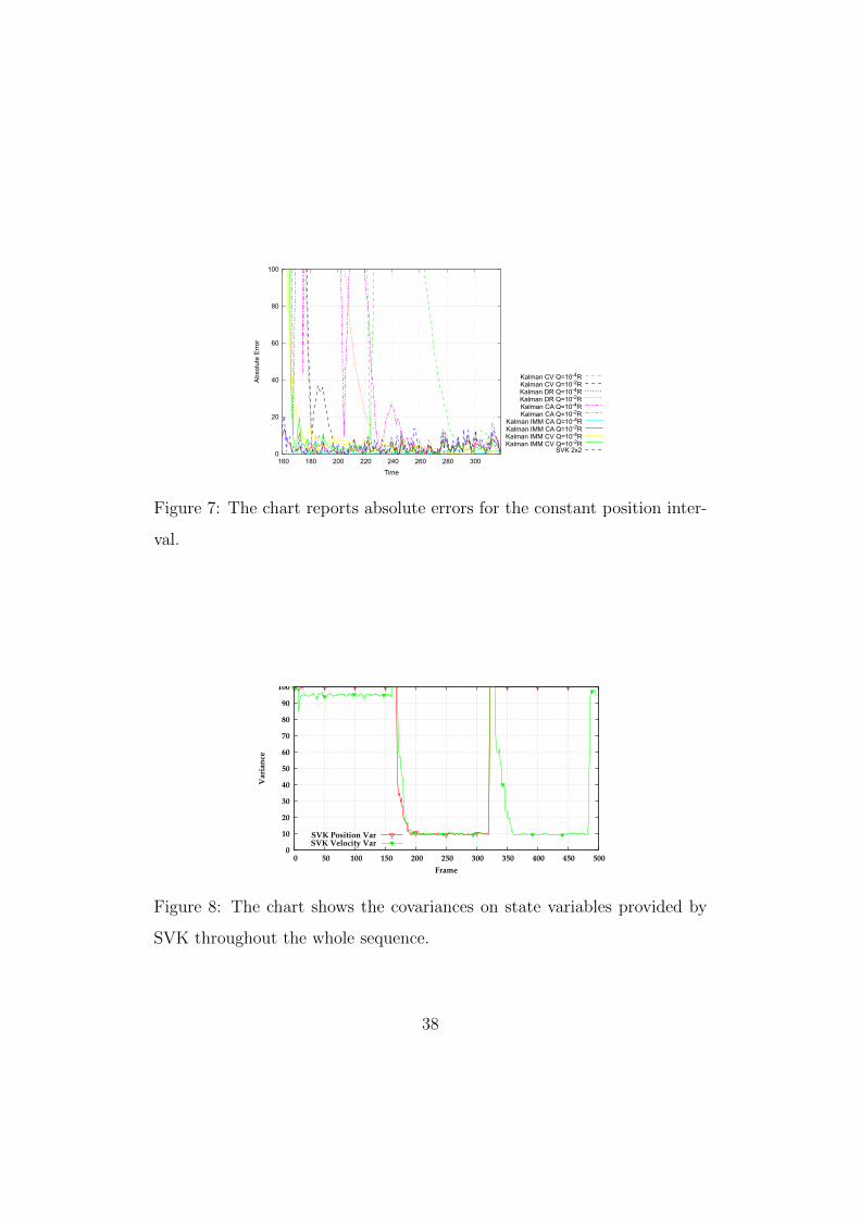
to its higher responsiveness. This is confirmed by Fig. 8, showing the po-

sition and the velocity variances estimated by SVK. It can be seen that,

immediately after the change of motion law from constant position to con-

stant velocity at sample 320, both variances significantly increase, somehow

”detecting” such a change, thanks to the adaptive process noise modeling

embodied into our filter. The resulting lower confidence in its predictions

automatically turns the filter from smoothness to responsiveness, prevent-

23

Filter Whole CA CV Drift CA* CV* Drift*

SVK 2x2 Model 22.41 9.79 38.02 35.41 8.91 9.63 1.67

Kalman IMM CA Q = 10−2R 18.23 4.62 31.62 3.61 4.50 4.22 4.62

Kalman IMM CA Q = 10−4R 60.21 4.6 105.43 1.79 4.48 3.41 1.40

Kalman IMM CV Q = 10−2R 56.03 76.91 36.78 44.82 102.86 4.37 4.36

Kalman IMM CV Q = 10−4R 76.05 69.78 87.37 72.52 89.34 2.92 3.62

Kalman CA Q = 10−2R 76.62 4.83 51.3 125.87 4.59 4.55 6.06

Kalman CA Q = 10−4R 357.45 4.26 242.19 581.52 3.72 4.04 7.87

Kalman CV Q = 10−2R 227.38 100.12 155.13 355.71 104.84 3.74 5.31

Kalman CV Q = 10−4R 1680.37 1213.78 1160.73 2439.37 1416.30 49.82 109.30

Kalman DR Q = 10−2R 4498.51 6015.22 4536.67 1793.30 8056.45 4757.75 2.77

Kalman DR Q = 10−4R 29698.38 25771.38 31583.97 29279.53 35763.45 37809.42 16743.08

Table 1: Comparison of RMSE on linear motion: first column reports the

RMSEs on the whole sequence; then, partial RMSEs on each piece of motion

are given as well as RMSEs concerning only the final part of each interval

(marked with *), when the filter may have reached the steady state.

ing the overshots/undershots exhibited by standard Kalman filters. After a

few samples, the covariance on the velocity decreases again, vouching that

SVK has confidently learned the new model. Between IMM filters, only re-

sponsive ones perform well during this interval, due to the delay in reacting

to the sharp change of smooth versions. Conversely, considering only the

steady state (6-th column of tab.1), smooth filters are best, since they more

effectively filter measurement noise. This is another strong indication of

the importance of adapting the covariance matrix on-line to achieve good

performance in every working condition. Considering only the steady state,

Kalman CV exhibits, as expected, good performance. Unlike the CA inter-

val, however, only the responsive tuning performs well since the smoother

Kalman CV has accumulated too much delay to recover. This difference is

24

due to the intrinsically higher smoothness of the CV model with respect to

CA. Kalman CA, with both tunings, is another good performer during the

steady state phase and this is also reasonable since a constant velocity mo-

tion may be seen as a special case of constant acceleration. Again, even in

this phase SVK is by far closer to the optimal filters than to those adopting

a wrong motion model and, visualizing only errors less than 50, it is the

only one visible in Fig. 6, apart from those correctly tuned.

Finally, due to the delay accumulated by the other filters, SVK turns

out the third best estimator in the constant position interval (4-th column

of Tab.1). Only the optimally tuned IMM CA filters perform better. Note

that, although IMM CV are optimally equipped for this interval, it comes

immediately after the CA interval. Hence, the CV filters have to recover

from accumulated delays and this results in a low global RMSE. Indeed,as

far as the steady state is concerned, all the filters exhibit a good RMSE apart

from very smooth ones, namely CV and DR tuned towards smoothness,

since they do not recover from delays even after 80 samples. Unlike the other

motion intervals, SVK keeps on being the best performer together with IMM

CA, even when only the steady state is considered. An explanation for this

is provided again by the chart of covariances (Fig. 8). During the constant

position part, the SVR is able to regress a very good transition matrix and

both the uncertainties are kept really low compared to the values in R.

Therefore, the filter is highly smooth, as can be observed in the chart of

absolute errors, and this keeps the RMSE low also in the last 80 frames.

Our proposal is robust to higher measurement noise, too. We report

in Tab.2 the RMSEs for the same simulation, but with R = 1000I. Even

in this case SVK turns out to be the overall second best thanks to its

25

Filter Whole CA Drift CV CA* Drift* CV*

SVK 2x2 Model R=1000 43.36 31.35 9.33 67.93 28.29 5.23 30.56

Kalman IMM CA Q = 10−2R 27.99 15.62 11.44 45.04 16.27 13.37 14.60

Kalman IMM CA Q = 10−4R 111.47 15.78 5.66 195.15 16.57 17.27 10.47

Kalman IMM CV Q = 10−2R 54.18 61.06 42.45 53.82 74.26 13.79 13.7

Kalman IMM CV Q = 10−4R 116.60 105.94 28.87 173.47 105.36 19.17 83.12

Kalman CA Q = 10−2R 79.65 15.36 130.17 52.94 14.52 19.17 14.3

Kalman CA Q = 10−4R 357.69 13.33 581.70 242.46 11.75 17.28 10.94

Kalman CV Q = 10−2R 228.08 100.97 356.26 156.61 106.77 16.81 11.71

Kalman CV Q = 10−4R 1681.04 1214.90 2439.48 1162.36 1418.82 106.66 49.56

Kalman DR Q = 10−2R 4500.00 6016.82 1793.01 4539.23 8059.09 8.78 4761.46

Kalman DR Q = 10−4R 29699.11 25772.48 29279.76 31584.70 35764.94 16742.06 37810.78

Table 2: Comparison of RMSE between different filters in case of higher

measurement noise.

adaptive behavior. Considerations similar to previous ones apply to the

three different parts of motion.

To summarize, simulations with linear motion laws show that the pro-

posed SVR-based approach to on-line adaptation of the transition model

is an effective solution for the tracking problem when the assumption of

stationary transition matrix cannot hold due to the tracked system under-

going significant changes in its motion traits. They also show that trying to

cope with the limited knowledge on the real transition model by deploying

multiple approximate models with IMM filters is prone to obtain the same

unsatisfactory performance when the right model is not present into the

pool, beside requiring to guess a larger set of parameters, such as especially

covariance matrices.

7.2. Simulation of non-linear motion

Given its ability to dynamically adapt the transition matrix, we expect

SVK to be superior to a standard Kalman filter or to IMM filters in the26

R = 100 Whole R=1000 Whole

SVK 2x2 Model 20.61 SVK 2x2 Model 43.84

Kalman IMM CA Q = 10−2R 38.53 Kalman IMM CA Q = 10−2R 44.71

Kalman IMM CA Q = 10−4R 48.88 Kalman IMM CA Q = 10−4R 58.23

Kalman IMM CV Q = 10−2R 289.90 Kalman IMM CV Q = 10−2R 242.67

Kalman IMM CV Q = 10−4R 236.11 Kalman IMM CV Q = 10−4R 215.54

Kalman CA Q = 10−2R 61.92 Kalman CA Q = 10−2R 62.32

Kalman CA Q = 10−4R 308.32 Kalman CA Q = 10−4R 308.66

Kalman CV Q = 10−2R 72.69 Kalman CV Q = 10−2R 72.95

Kalman CV Q = 10−4R 248.30 Kalman CV Q = 10−4R 248.46

Kalman DR Q = 10−2R 143.63 Kalman DR Q = 10−2R 144.87

Kalman DR Q = 10−4R 434.83 Kalman DR Q = 10−4R 435.20

Table 3: Comparison of RMSE in case of non-linear motion.

case of non-linear motion. In such a case, in fact, a time-varying linear

function can approximate better than a fixed linear function the real non-

linear motion. Hence, to test this conjecture we have run simulations with

a motion compound of two different sinusoidal parts linked by a constant

position interval. The motion law of the two sinusoidal parts is as follows:

x1(t) = 300t+ 300 sin(2πt) + 300 cos(2πt), (15)

x2(t) = 300t− 300 sin(2πt)− 300 cos(2πt). (16)

Aggregate results are shown in Fig. 9, Fig. 10 and Tab.3 for the same levels

of measurement noise as in 7.1. In this case our filter proves to be the overall

best, indeed confirming its superior flexibility.

8. Experimental results

In this section we provide experimental results on real data. The ex-

periments concern 3D camera tracking and target tracking onto the image27

plane. For target tracker onto the image plane, we also provide quantitative

results.

8.1. 3D camera tracking

In this experiment, we track the 3D position of a moving camera in or-

der to augment the video content, taking as measurement the output of a

standard camera pose estimation algorithm [29] fed with point correspon-

dences established matching invariant local features, in particular SURF

features [30]. Some snapshots are reported in Fig. 11. The snapshots show

side-by-side the augmentation resulting from the use of Kalman CA (top

image) and our SVK filter (bottom image). Both filters have been tuned

to be as responsive as in 7.2 and measurement noise covariances has been

adjusted to match the range of the input data. The sequence shows a fast

change of motion of the camera, the purpose of filters being to keep the vir-

tual object spatially aligned with the reference position, denoted for easier

interpretation of results by a white sheet of paper. We can see that both

filters exhibit a delay following the sharp motion change at frame 19, but

SVK is subject to a much smaller translation error (e.g. frame 23), recovers

much faster (SVK is again on the target by frame 27, Kalman CA only by

frame 40) and, unlike Kalman CA, without any overshot (which Kalman

CA exhibits from frames 27 to 40).

8.2. Tracking onto the image plane: qualitative evaluation

In this experiments, we compare qualitatively our SVK to standard,

non adaptive solutions for estimating an object trajectory in the image

plane based on the mean-shift tracker introduced in [1]. We compare the

28

original mean-shift (MS) tracker, the non-adaptive Kalman filter (Kalman-

MS tracker) and the IMM filter (IMM-MS tracker) to SVK. Kalman-MS,

IMM-MS as well as SVK deploy the MS tracker as source of measurements.

The MS tracker and the Kalman-MS tracker have been proposed in the

original paper on mean-shift [1].

The basic MS tracker implicitly assumes a constant position transition

model by letting the tracker start its search for the best position in each new

frame exactly at the position where the target was found in the previous

frame. Instead, the Kalman-MS tracker deployed in our experiment relies

on a constant velocity motion model and the IMM-MS tracker has both a

constant position and a constant velocity motion model.

Some snapshots of one test sequence are depicted in Fig. 12. The mean-

shift technique in general cannot withstand total occlusions, such as that

shown in the third snapshot (Frame # 069), because the MS tracker can

be attracted by the background structure (e.g. the road in our experiment)

if this turns out more similar to the target than the occluding object. For

this reason the MS Tracker is unwilling to follow the object while it passes

below the advertisement panel and stays in the last position where it could

locate the target (frame # 069 of Fig. 12). The Kalman-MS tracker and the

IMM-MS tracker follow the previous dynamics of the target, thanks to the

smoothness brought in by the transition models (frame # 069 of Fig. 12).

Nevertheless, since the way they weight the contribution of measurement

and prediction on the state is fixed, they are finally caught back by the

measurements (i.e. the MS tracker) continuously claiming the presence of

the target in the old location, before the occluding object. Only the SVK

is able to correctly guess the trajectory of the target while the latter is oc-

29

cluded (frame # 069 of Fig. 12) and continues to track it after the occlusion

(frame # 084 and subsequent frames of Fig. 12). This is due to the abil-

ity of the SVK to dynamically adjust the process noise covariance matrix,

increasing its confidence on the motion of the object (i.e. to decrease the

variance) while the object keeps moving with an approximatively constant

motion law on the image plane (first part of the sequence, first two snap-

shots, from frame # 001 to frame # 051 of Fig. 12). Thanks to the high

confidence gained on its motion model, the filter can reject the wrong mea-

surements coming from the MS tracker during the occlusion. This happens

again during the second occlusions at frame # 201 of Fig. 12.

Similar considerations apply to the test sequence depicted in Fig. 13.

Thanks to its adaptive behavior, SVK lets the mean shift tracker producing

the new measurement at frame # 86 start more on the left than the other

two trackers, i.e. the filter has learned that the target is slowing down and

exploits this adaptive knowledge to guide the measurements. This allows

the mean shift tracker used by the SVK filter to recover the target as soon

as it is not occluded (frame # 101) and to stick to it during the subsequent

frames (e.g. # 127 and # 195). In this sequence, which is less challenging

than the previous one as the occlusion lasts less, the higher flexibility on

the transition model of the IMM-MS tracker with respect to the simple

Kalman-MS allows it to exhibit similar performance to that of the SVK.

8.3. Tracking onto the image plane: quantitative evaluation

To perform a quantitative comparison with non-adaptive methods, we

used the methodology recently introduced in [31] and two sequences, Faceocc2

30

and DavidIndoor, from a publicly available dataset1 introduced in two re-

cent and very relevant proposals of adaptive appearance model trackers. We

chose the methodology presented in [31] because it allows to compare meth-

ods independently of thresholds: it compares algorithms by simultaneously

considering the mean Dice overlap and the Correct Track Ratio, i.e. the

percentage of frames of a sequence that the tracker overlap is above a given

threshold. This pair of values is plotted for every possible threshold value,

resulting in curves like those depicted in Fig. 14: the higher the curve, the

better the tracker performance. For more details on this methodology and

the analyses that can be carried out on such curves, the reader is referred

to [31].

The SVK turns out the best in both sequences. Only on Faceocc2, the

IMM filter offers similar performance. These sequences are designed to test

appearance adaptive trackers. The mean-shift tracker, upon which all the

evaluated trackers are based, is not adaptive: this is especially evident on

the DavidIndoor sequence, where the target appearance between the first

frame and the middle of the sequence changes drastically. This change of

appearance makes all the trackers drift away from the target: the only one

to remain on-target is the SVK, due to the high confidence gained on the

target motion model, which overrules the wrong measures received from the

Mean-shift tracker. In Faceocc2, where the greatest challenge is represented

by partial occlusions, the mean-shift tracker is more effective. Nevertheless,

trackers like IMM-MS and SVK, that offer time-variant transition models,

obtain better performance than the basic algorithm. It is worth noting that

our filter obtains the same performance of IMM-MS while requiring to set

1http://vision.ucsd.edu/~bbabenko/project_miltrack.shtml

31

a lot less parameters.

9. Parameters sensitivity

To conclude the experimental validation of our proposal, we present

a study about the sensitivity of the proposed algorithm to the parameter

values. We used the DavidIndoor sequence presented in the previous section

and consider the parameters W , i.e. the size of the sliding window, and C,

i.e. the regularization term multiplier in the SVR objective function.

Results are reported in Fig. 15. We studied the effects of the parameters

separately: in particular, we kept one parameter equal to the value used in

the previous evaluation, and let the other vary. We report the mean Dice

overlap over the whole sequence for the different parameter combinations.

The proposed filter turns out robust to parameter tuning. In particular, the

sliding window size is not a critical parameter, as the filter attains similar

Dice overlaps even with small W , i.e. when it is provided with limited

samples to regress a meaningful transition model. Similarly, the algorithm

is not particularly sensitive to the value of C, as long as it is small enough

to assign to the regressed transition model a low uncertainty, as explained

in Sec. 6.2.

10. Conclusions

A new approach to build an adaptive recursive Bayesian estimation

framework has been introduced, both from a theoretical point of view and

in terms of its instantiation in the case of linear transition and measurement

models and Gaussian noise. The proposed SVK filter has been shown to

32

outperform a standard Kalman filter and an IMM filter while also requiring

less parameters to be arbitrarily (and possibly wrongly) tuned.

It has also been highlighted how the proposed approach can be seen

as a novel and general on-line adaptive Kalman filtering algorithm and

thus beneficially deployable in a variety of hidden state estimation problems

relying on different measurement sources, such as e.g. target tracking in

the image plane based on color histograms and mean shift optimization as

well as camera tracking based on interest points matching and camera pose

estimation.

Endowing the vision of this work as a step towards a general and param-

eters free tracking system, an interesting future direction of research may

deal with the insertion of algorithms for automatic on-line selection of SVR

parameters. Finally, the instantiation of our proposal also in the case of non

linear and non Gaussian tracking, in particular by modifying it in order to

be beneficially used also with particle filters, would be a major contribution

to foster its applicability and adoption.

References

[1] D. Comaniciu, V. Ramesh, P. Meer, Kernel-based object tracking, Transactions on

Pattern Analysis and Machine Intelligence (PAMI) 25 (2003) 564–575.

[2] B. Ristic, S. Arulampalam, N. Gordon, Beyond the Kalman Filter: Particle Filters

for Tracking Applications, Artech House, Boston, MA, USA, 2004.

[3] A. J. Smola, B. S. Olkopf, A tutorial on Support Vector Regression, Technical

Report, Statistics and Computing, 1998.

[4] S. Salti, D. Luigi, On-line learning of the transition model for recursive bayesian

estimation, in: Proc. of the 2nd International Workshop on Machine Learning for

Vision-based Motion Analysis (MLVMA).

33

[5] R. E. Kalman, A new approach to linear filtering and prediction problems, Trans-

actions of the American Society of Mechanical Engineers (ASME)–Journal of Basic

Engineering 82 (1960) 35–45.

[6] A. Adam, E. Rivlin, I. Shimshoni, Robust Fragments-based Tracking Using the Inte-

gral Histogram, in: Proc. of the Computer Society Conference on Computer Vision

and Pattern Recognition (CVPR) - Volume 1, IEEE Computer Society Washington,

DC, USA, 2006, pp. 798–805.

[7] S. Avidan, Ensemble tracking, in: Proc. of the International Conference on Com-

puter Vision and Pattern Recognition (CVPR) - Volume 2, IEEE Computer Society

Washington, DC, USA, 2005, pp. 494–501.

[8] R. T. Collins, Y. Liu, M. Leordeanu, Online Selection of Discriminative Tracking

Features., Transactions on Pattern Analysis and Machine Intelligence (PAMI) 27

(2005) 1631–43.

[9] M. Harville, D. Li, Fast, integrated person tracking and activity recognition with

plan-view templates from a single stereo camera, in: Proc. of the Computer Society

Conference on Computer Vision and Pattern Recognition (CVPR) - Volume 2, IEEE

Computer Society, Washington, DC, USA, 2004, pp. 398–405.

[10] M. Isard, J. MacCormick, BraMBLe: A bayesian multiple-blob tracker, in: Proc.

of the International Conference on Computer Vision (ICCV) - Volume 2, IEEE

Computer Society, Washington, DC, USA, 2001, pp. 34–41.

[11] I. Haritaoglu, D. Harwood, L. S. Davis, W4: Real-time surveillance of people and

their activities, Transactions on Pattern Analysis and Machine Intelligence (PAMI)

22 (2000) 809–830.

[12] P. Prez, C. Hue, J. Vermaak, M. Gangnet, Proc. of the color-based probabilistic

tracking, in: Proceedings of the Seventh European Conference on Computer Vision

(ECCV) - Part I, Lecture Notes in Computer Science (LNCS), Springer-Verlag,

London, 2002, pp. 661–675.

[13] R. Mehra, Approaches to adaptive filtering, Transactions on Automatic Control 17

(1972) 693–698.

[14] M. Oussalah, J. De Schutter, Adaptive Kalman filter for noise identification, in:

Proc. of the 25th International Conference on Noise and Vibration Engineering

34

(ISMA), Katholieke Universiteit, Leuven, Belgium, 2000, pp. 1225–1232.

[15] Y. Liang, D. X. An, D. H. Zhou, Q. Pan, A finite-horizon adaptive Kalman filter for

linear systems with unknown disturbances, Signal Processing 84 (2004) 2175–2194.

[16] S.-K. Weng, C.-M. Kuo, S.-K. Tu, Video object tracking using adaptive Kalman

filter, Journal of Visual Communication and Image Representation 17 (2006) 1190–

1208.

[17] Y. Zhang, H. Hu, H. Zhou, Study on adaptive Kalman filtering algorithms in human

movement tracking, in: Proc. of the IEEE International Conference on Information

Acquisition (ICIA), pp. 11–15.

[18] E. Mazor, A. Averbuch, Y. Bar-Shalom, J. Dayan, Interacting multiple model meth-

ods in target tracking: a survey, IEEE Transactions on Aerospace and Electronic

Systems 34 (1998) 103–123.

[19] M. E. Farmer, R.-L. Hsu, A. K. Jain, Interacting multiple model (IMM) Kalman

filters for robust high speed human motion tracking, in: International Conference

on Pattern Recognition, volume 2, IEEE, 2002, pp. 20–23.

[20] J. Burlet, O. Aycard, A. Spalanzani, C. Laugier, Pedestrian tracking in car parks:

an adaptive interacting multiple models based filtering method, in: Intelligent

Transportation Systems Conference, IEEE, 2006, pp. 462–467.

[21] V. N. Vapnik, The Nature of Statistical Learning Theory, Springer-Verlag, New

York, NY, USA, 1995.

[22] M. Pontil, S. Murkerjee, F. Girosi, On the Noise Model of Support Vector Machine

Regression, Technical Report, Massachusetts Institute of Technology, Cambridge,

MA, USA, 1998.

[23] L. Cao, Q. Gu, Dynamic Support Vector Machines for non-stationary time series

forecasting, Intelligent Data Analysis 6 (2002) 67–83.

[24] T. Poggio, S. Mukherjee, R. Rifkin, A. Rakhlin, A. Verri, b, Technical Report CBCL

Paper 198/AI Memo 2001-011, Massachusetts Insititute of Technology, Artificial

Intelligence Laboratory, 2001.

[25] J. C. Platt, Fast Training of Support Vector Machines Using Sequential Minimal

Optimization, MIT Press, MA, USA, Cambridge, MA, USA, pp. 185–208.

[26] J. Gao, S. Gunn, C. Harris, M. Brown, A probabilistic framework for SVM regression

35

and error bar estimation, Machine Learning 46 (2 January 2002) 71–89.

[27] W. Chu, S. Keerthi, C. J. Ong, Bayesian Support Vector Regression using a unified

loss function, Transactions on Neural Networks 15 (2004) 29–44.

[28] C.-J. Lin, R. C. Weng, Simple Probabilistic Predictions for Support Vector Regres-

sion, Technical Report, Department of Computer Science, National Taiwan Univer-

sity, 2004.

[29] G. Schweighofer, A. Pinz, Robust pose estimation from a planar target, Transactions

on Pattern Analysis and Machine Intelligence (PAMI) 28 (2006) 2024–2030.

[30] H. Bay, A. Ess, T. Tuytelaars, L. J. V. Gool, Speeded-Up Robust Features (SURF),

Computer Vision and Image Understanding 110 (2008) 346–359.

[31] S. Salti, A. Cavallaro, L. Di Stefano, Adaptive Appearance Modeling for Video

Tracking: Survey and Evaluation, Trans. on Image Processing (2012 (to appear)).

36

Algorithm 1 RBE with on-line transition model adaptation

INPUT: a set of noisy measurements, Z1:K = {zk}Kk=1

INPUT: an initial state PDF, p(x0)

OUTPUT: the estimated trajectory in the state space, X̂1:K = {x̂k}Kk=1

// Bootstrap

p(x̂1) = RBE Predict(p(x0))

p(x1) = RBE Update(p(x̂1), z1)

for k = 2 : W do

for i = 1 : n do

p(x̂k) = RBE Predict(p(xk−1))

p(xk) = RBE Update(p(x̂k), zk)

SV R[i].addTrainingSample(xk−1, xk[i], k)

end for

end for

// Main loop

for k ∈ W + 1 : K do

for i ∈ 1 : n do

p(x̂k) = RBE Predict(p(xk−1))

p(xk) = RBE Update(p(x̂k), zk))

removeOldestTrainingSample(SV R[i])

addTrainingSample(SV R[i],xk−1,xk[i], k)

SV R[i].train(F̂k+1[i, :], Q̂k+1[i, i])

p(x̂k) = RBE SetTransitionModel(F̂k+1[i, :], Q̂k+1[i, i])

end for

end for

37

0

20

40

60

80

100

160 180 200 220 240 260 280 300

Abs

olut

e E

rror

Time

Kalman CV Q=10-4RKalman CV Q=10-2RKalman DR Q=10-4RKalman DR Q=10-2RKalman CA Q=10-4RKalman CA Q=10-2R

Kalman IMM CA Q=10-4RKalman IMM CA Q=10-2RKalman IMM CV Q=10-4RKalman IMM CV Q=10-2R

SVK 2x2

Figure 7: The chart reports absolute errors for the constant position inter-

val.

0

10

20

30

40

50

60

70

80

90

100

0 50 100 150 200 250 300 350 400 450 500

Vari

an

ce

Frame

SVK Position VarSVK Velocity Var

Figure 8: The chart shows the covariances on state variables provided by

SVK throughout the whole sequence.

38

-1500

-1000

-500

0

500

1000

1500

2000

2500

0 50 100 150 200 250 300 350 400 450 500

Pos

ition

Time

Ground-truthKalman CV Q=10-4RKalman DR Q=10-4RKalman CA Q=10-4R

Kalman IMM CA Q=10-4RKalman IMM CV Q=10-4R

SVK 2x2

-1000

-500

0

500

1000

1500

2000

2500

3000

0 50 100 150 200 250 300 350 400 450 500

Pos

ition

Time

Ground-truthKalman CV Q=10-2RKalman DR Q=10-2RKalman CA Q=10-2R

Kalman IMM CA Q=10-2RKalman IMM CV Q=10-2R

SVK 2x2

Figure 9: Simulation dealing with non-linear motion with R = 100I. Chart

on top compares SVK to Kalman filters tuned for smoothness, the bottom

one to Kalman filters tuned for responsiveness. At this scale, the estimation

of our filter is almost indistinguishable from the ground truth.

39

-500

0

500

1000

1500

2000

0 50 100 150 200 250 300 350 400 450 500

Pos

ition

Time

Ground-truthKalman CV Q=10-4RKalman DR Q=10-4RKalman CA Q=10-4R

Kalman IMM CA Q=10-4RKalman IMM CV Q=10-4R

SVK 2x2

-1000

-500

0

500

1000

1500

2000

2500

3000

0 50 100 150 200 250 300 350 400 450 500

Pos

ition

Time

Ground-truthKalman CV Q=10-2RKalman DR Q=10-2RKalman CA Q=10-2R

Kalman IMM CA Q=10-2RKalman IMM CV Q=10-2R

SVK 2x2

Figure 10: Simulation dealing with non-linear motion with R = 1000I.

Chart on top compares SVK to Kalman filters tuned for smoothness, the

bottom one to Kalman filters tuned for responsiveness.

40

(a) 17 cropped (b) 21 cropped

(c) 23 cropped (d) 25 cropped

(e) 27 cropped (f) 28 cropped

(g) 34 cropped (h) 40 cropped

Figure 11: Some of the most significant frames (top: Kalman CA, bottom:

SVK) from the 3D camera tracking experiment.

41

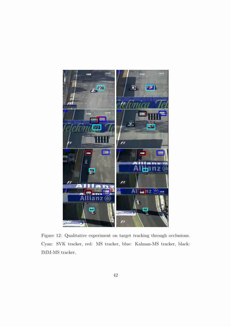
Figure 12: Qualitative experiment on target tracking through occlusions.

Cyan: SVK tracker, red: MS tracker, blue: Kalman-MS tracker, black:

IMM-MS tracker.

42

Figure 13: Qualitative experiment on target tracking through occlusions.

Cyan: SVK tracker, red: MS tracker, blue: Kalman-MS tracker, black:

IMM-MS tracker.

43

0

0.2

0.4

0.6

0.8

1

0 0.2 0.4 0.6 0.8 1

Mea

n D

ice

Correct Track Ratio

0

0.2

0.4

0.6

0.8

1

0 0.2 0.4 0.6 0.8 1

Mea

n D

ice

Correct Track Ratio

(a) (b)

Figure 14: Quantitative results. From top to bottom: quantitative results,

first frame, exemplar frame from the sequence. (a) Faceocc2 sequence; (b)

DavidIndoor sequence.

44

0

0.05

0.1

0.15

0.2

0.25

0.3

0.0001 0.001 0.01 0.1 1

Dice Overlap

C

SVKalmanMS W=10

0

0.05

0.1

0.15

0.2

0.25

0.3

6 8 10 12 14 16 18 20

Dice Overlap

W

SVKalmanMS C=0.01

Figure 15: Sensitivity of the proposed algorithm with respect to parameters

value.

45