on local and zonal pulses of atmospheric heat transport in...
TRANSCRIPT

Quarterly Journal of the Royal Meteorological Society Q. J. R. Meteorol. Soc. 141: 2376–2389, July 2015 B DOI:10.1002/qj.2529
On local and zonal pulses of atmospheric heat transport in reanalysisdata
G. Messori* and A. CzajaSpace and Atmospheric Physics Group, Department of Physics, Imperial College London, UK
*Correspondence to: G. Messori, Department of Meteorology, Stockholm University, 16c, Svante Arrhenius vag,106 91 Stockholm, Sweden.
E-mail: [email protected]
The present study analyses large values (or pulses) of local and zonally integrated meridionalatmospheric heat transport due to transient eddies. The data used is the European Centrefor Medium-range Weather Forecasts ERA-Interim reanalysis with daily, 0.7◦ latitudeand longitude resolution. The domain of interest is the extratropics. First, the circulationassociated with local pulses of heat transport is described. This is found to match many ofthe features found in warm conveyor belts, although important regional differences exist.The large values of heat transport are seen to be associated with co-varying meridionalvelocity and moist static energy anomalies. Next, it is shown that there exist strong pulses ofmeridional heat transport when a zonal integral around a given latitude circle is considered.These zonal pulses are only partly driven by the synchronized occurrence of a large numberof local pulses. The existence of such pronounced variability in zonally integrated meridionalheat transport can have important consequences for the energy balance of the high latitudes.
Key Words: heat transport; atmosphere; transport pulse; extreme events; reanalysis; variability; transient motions
Received 7 May 2014; Revised 21 January 2015; Accepted 4 February 2015; Published online in Wiley Online Library 02April 2015
1. Introduction
As part of the vast body of literature dedicated to anthropogenicclimate change, a great deal of attention has focused on possiblechanges in the magnitude and drivers of meridional heat transport(e.g., Hwang and Frierson, 2010; Zelinka et al., 2012). Althoughthere is some agreement on the general trends, the transportmagnitudes forecasted by models for both pre-industrial andfuture scenarios are extremely variable (e.g., Donohoe and Battisti,2012; Zelinka et al., 2012).
In many cases, the focus is on zonally integrated, time-meantransport values. The role of variability on subseasonal time-scales has received comparatively little attention. At the sametime, atmospheric heat transport is known to be sensitive toshort-lived, very intense heat bursts. Swanson and Pierrehumbert(1997) were among the first to highlight the important role playedby extreme events in atmospheric heat transport by transientmotions, using data from three locations in the Pacific stormtrack. Messori and Czaja (2013, hereafter MC13; 2014) havegeneralized this conclusion showing that, at any given location inthe extratropical regions during both winter and summer, only avery few days every season can account for over half of the netseasonal transport. The mean transport by transient motions istherefore effectively set by a few extreme events every season.
The above studies focused on a local view of the transport,whereby the calculations were based on transport values atsingle grid boxes. The discussion was centred on statisticalfeatures of the transport and local processes; relatively little
attention was devoted to analysing the larger-scale circulationassociated with the extremes. If the local extremes were associatedwith systematic mesoscale, synoptic or larger-scale circulationfeatures, this might lead to a measure of synchronization betweenevents at different longitudes. We will refer to these zonallysynchronized events as ‘zonal extremes’. Zonal extremes couldpotentially carry a significant amount of the net seasonal heattransport over a very short period of time. The meridionalatmospheric heat transport by transient motions might thereforebe characterized by a fundamentally sporadic nature, even whenadopting a zonally integrated view. Subseasonal anomalies inthe magnitude and convergence of atmospheric heat transportcan have severe impacts on the polar regions (Graversen et al.,2011). The existence of zonal extremes would therefore providean important new perspective on the study of meridional heattransport under a changing climate.
If zonal extremes were indeed found to exist, this would opena number of questions: how do local and zonal extremes relate toeach other? How will the frequency and intensity of zonal extremeschange in the future? How will this influence the polar regions?The present article will focus on the first of these questions, andaims to:
a. Provide a simple overview of the circulation featuresassociated with local extremes.
b. Demonstrate the existence of strong pulses of zonallyintegrated meridional heat transport across a given latitudecircle (i.e zonal extremes).
c© 2015 Royal Meteorological Society

Local and Zonal Pulses of Atmospheric Heat Transport 2377
c. Show that these zonal pulses are partly driven by thesynchronized occurrence of a large number of localextremes, and that this is consistent with the circulationfeatures discussed in point (a).
The focus is on atmospheric poleward heat transport by time-dependent motions in the ERA-Interim dataset. An analysis ofthe climate forecasts made by GCMs is beyond the scope of thisstudy, but the methodology presented here lays out the basis foran investigation on the subject.
First, the circulation associated with local pulses of heattransport is described. This is found to match many of thefeatures found in warm conveyor belts, although importantregional differences exist. The second part of the analysis iscentred on the largest zonally integrated values of meridionalheat transport. It is shown that the top percentiles of the zonallyintegrated transport distribution are significantly different fromall other days, and can therefore be considered zonal extremeevents. The discussion focuses on the relationship between thesezonal extremes and the local pulses. The structure of this articleis as follows. Section 2 describes the data used and outlinesthe methodology. Section 3 looks at the circulation associatedwith the local extremes. An analysis of the zonally integratedheat transport is presented in section 4, with a focus on thenature and role of the extreme events. Section 5 discusses therelationship between local and zonal extremes. Finally, section 6presents some further discussion, conclusions and scope for futureresearch.
2. Data and methods
2.1. The re-analysis data
The present study utilizes the European Centre for Medium-range Weather Forecasts (ECMWF) ERA-Interim reanalysis data(Simmons et al., 2006). Similar to MC13, daily (1200 UTC) fieldswith a 0.7◦ latitude and longitude resolution are considered. Asubset of the data has been analysed at six-hourly resolution toverify that the conclusions drawn are not dependent on the choiceof utilizing daily values. The period taken into consideration spansfrom June 1989 to February 2011, thereby providing 22 December,January and February (DJF) and 22 June, July and August (JJA)time series. Even though ERA-Interim includes additional yearsof data, this more limited period is selected to allow for an easycomparison with the analysis presented in Messori and Czaja(2014).
The analysis of the circulation features (section 3) uses allavailable pressure levels between 975 and 20 mb. The statisticalanalysis of the extreme events (sections 4 and 5) focuses on the850 mb level. This is the level of the peak heat transport bytransient eddies, and is often used as a reference level in theliterature (e.g., Lau, 1978). Other vertical levels in the data setwere analysed by MC13 and they found that the 850 mb analysisprovided a good indication of the statistics of the transport atother levels.
2.2. Meridional heat transport by transient motions
The transient-eddy transport is computed as the product ofv (meridional velocity) and H (moist static energy, hereafteralso referred to as MSE) temporal anomalies. These are definedas departures from the linearly detrended seasonal mean, andare denoted by a prime. Velocity is positive polewards in bothhemispheres. Moist static energy is defined as:
H = Lvq + CpT + gz, (1)
where Lv is the latent heat of vaporization, Cp is the specificheat capacity at constant pressure, T is the absolute temperature,q is the specific humidity, z is the geopotential height and g
is the gravitational acceleration (e.g., Neelin and Held, 1987).The anomalies are computed at every grid point for 172 latitudebands between 30◦N and 89◦N and 30◦S and 89◦S, and theanalysis is performed over both land and ocean.
The terminology ‘local event’ simply refers to the transportvalue at a single reanalysis grid box. In order to present resultsin the same units as the zonally integrated values, the localtransport in the figures has been multiplied by the circumferenceof the latitude at which it is located. Zonally integrated values arecomputed by integrating each local v′H′ value over the width ofthe grid box it refers to. All the values around a given latitude arethen summed to obtain the zonal integral. Both local and zonalvalues are then normalized by layer thickness, and the transport isexpressed in W/1000 hPa. Values therefore can be interpreted asthe transport in W that would occur if the local flux were realizedat all vertical levels and longitudes.
For both the local and zonally integrated analyses, extremeevents are defined as the values of v′H′ exceeding the 95thpercentiles of the respective distributions, for the full hemisphereand time period considered. Note that these distributions arecomputed for the 850 mb level only. It is shown by MC13 that theexact percentile chosen as threshold does not affect the statisticalcharacteristics of the extremes for single-point values. The sameis found in the case of the zonally integrated distributions.The sensitivity of the analysis to the extreme event threshold isdiscussed further in section 5.5.
Part of the analysis is performed on time-filtered data. The filterused is a 21-point high-pass finite impulse response filter, witha half-power cut-off at 8 days. It is designed to capture the fullbreadth of baroclinic time-scales. Chang (1993) suggested thatfilters with a 6 day cut-off lose a key part of the baroclinic variance.Here, we therefore follow Nakamura et al. (2002) in choosing an8 day cut-off. Where no filter is applied, the analysis encompassesphenomena covering a wide range of periods, beyond thosetypically associated with baroclinic time-scales. A brief discussionof the sensitivity of the present analysis to filtering is thereforeprovided in the online Supporting Information (File S2).
The analysis also includes ‘well-separated’ local extremes. Theseare local extremes that are driven by distinct atmospheric systemsas opposed to extremes resulting from a single, zonally elongatedregion of enhanced transport, which might register as a localextreme at several locations. In order to provide an objectivedefinition of well-separated extremes, a mean decorrelationlength scale for the heat transport is computed at every latitude.The decorrelation scale is defined as the distance over whichthe autocovariance function of the transport anomalies crosseszero for the first time. Local extremes that are more than onedecorrelation scale apart are counted separately. If multipleextremes are within one decorrelation scale of each other, thegroup is counted only once.
2.3. Two-dimensional heat transport cross-sections
The analysis of the circulation features (section 3) is based oncross-sectional composites of local extreme events in the zonaland height (pressure) plane. The selection of these extremes isbased on the transport values at single data points, with no zonalintegration applied. In all of the composite figures, only theextremes corresponding to local maxima are selected. If only asimple percentile threshold were applied, an extensive region ofstrong heat transport could contribute with multiple data pointsto the statistics. This is desirable when computing, for example,a climatology of heat transport bursts. However, it becomesproblematic when analysing atmospheric circulation, because itwould artificially replicate the circulation system associated witha single heat transport peak.
In MC13, the majority of local events were found to havezonal wave numbers between 6 and 10. In order to capture thefull extent of the extremes, including the surrounding circulationfeatures, 50 reanalysis grid boxes (corresponding to approximately
c© 2015 Royal Meteorological Society Q. J. R. Meteorol. Soc. 141: 2376–2389 (2015)

2378 G. Messori and A. Czaja
35◦ longitude), are retained on either side of the selected localmaxima. To avoid double-counting data points, if two extremesoccur on the same day and latitude and are less than 100 gridboxes apart, half the grid boxes in the interval are assignedto each of the extremes. The heat transport is then computedacross all the selected longitude data points, at all pressure levels.This procedure provides a pressure–longitude transport cross-section for each extreme. All the extremes thus analysed are thencomposited, and the values found are normalized by the numberof data points in the composite. Note that, because some extremesare less than 100 grid boxes apart, the normalization factor will notbe uniform across the composite. A similar procedure is applied toobtain cross-sectional plots of the wind fields corresponding to theextreme events. Note that no vertical integration is performed.Indeed, the reanalysis estimates might not be accurate for thewhole vertical extent between two adjacent pressure levels. Asnoted by Trenberth (1991), the values archived in the ECMWFreanalyses should be interpreted as the most accurate valuesavailable at those levels, but not representative of layers. Suchan issue has vastly improved in the passage from ERA-40 toERA-Interim, but is still present in the latter data set and shouldnot be ignored (e.g., Graversen et al., 2011).
Since the atmospheric circulation is analysed using compositeplots, one needs to ensure that the mean picture representsindividual events well. As a first step, statistical significance limitsare presented in the cross-sectional plots. The null hypothesis isthat the structure of the extreme events does not differ significantlyfrom that of all other poleward transport events. Events above the75th percentile of the full hemispheric distribution are taken asreference for the average event. A random Monte-Carlo sampling(1000 iterations) is then performed to determine locations wherethe extreme event composite is not statistically different fromthe average events at the 99% confidence level. A separate testis performed exclusively on the areas that display equatorward(negative) transport. Here, a non-parametric sign test is applied,with the null hypothesis that the data in these regions comesfrom an unknown distribution with a positive median. Again,a 99% confidence threshold is considered. The first test verifieswhether the extreme event composite is statistically differentfrom the weaker poleward transport instances. The second testevaluates whether the negative transport is a robust featureof the extremes or whether it is simply part of a near-zerobackground flow. The same procedure is applied to the velocitycomposites.
In addition to this, two further analyses are performed. In thefirst, extreme events are split into those corresponding to polewardvelocity anomalies and those corresponding to equatorward ones.The second analysis focuses on regional domains, selected so as tomatch the areas in which local extreme events are most frequent.The names of the different domains, and the correspondinggeographical boundaries, are listed in Table 1. Figure 6(a) providesa graphical illustration of the same domains.
2.4. Net meridional heat transport and probability densityfunctions
In addition to the transport by transient motions described above,we also briefly analyse the net, vertically and zonally integratedmeridional heat transport by all atmospheric motions. This is
Table 1. Names, abbreviations and geographical boundaries of the domains usedin the analysis of extreme event regional composites.
Domain name Abbreviation Boundaries
a. Gulf Stream GS 30◦N–55◦N; 265◦E–335◦Eb. Pacific Storm Track PS 30◦N–50◦N; 150◦E–230◦Ec. Bering Strait/Gulf of Alaska BS 55◦N–70◦N; 180◦E–200◦Ed. Nordic Seas NS 55◦N–80◦N; 335◦E–15◦Ee. Southern Ocean SO 40◦S–70◦S; 295◦E–275◦E
expressed as:
TATM = 1
g
1∫0
dη
2π∫0
dφv
(1
2u·u + CpT + gz + Lvq
)∂p
∂η, (2)
where g is gravity, u = (u, v) is the horizontal wind vector, p isthe pressure, φ is the longitude and η is the vertical coordinate ofthe ERA-Interim atmospheric model (Graversen et al., 2011). TheTATM provides a value in W for the net northward energy transportacross a given latitude circle. A barotropic mass correction is alsoapplied, following Trenberth (1991) and Graversen (2006). Thisaccounts for the non-conservation of mass in the ERA-Interimdataset.
Finally, the present article discusses several probability densityfunctions (PDFs), and refers to their skewness. This is a measureof the asymmetry of a distribution or, more formally, thedistribution’s third standardized moment. Note that a skewnessof zero does not necessarily imply symmetry about the mean.Another oft-used indicator is the most likely value (MLV) of thePDF, which is taken to be the central value of the bin with thehighest frequency of events. The exact value of the MLV obviouslydepends on the choice of bins. Nonetheless, the MLV is generallya robust indicator if used to compare the order of magnitudeof the most frequent value of a variable to the one of its mostextreme outcomes.
3. Atmospheric circulation and local extremes
Previous studies (e.g., Swanson and Pierrehumbert, 1997; MC13;Messori and Czaja, 2014) have highlighted how meridionalatmospheric heat transport is sensitive to short-lived, very intenseheat bursts. Here, these are referred to as local extreme events (orpulses). The term ‘local’ simply refers to the transport at a singlegrid box. When analysing local transport, the extremes form apopulation of events that are one or more orders of magnitudelarger than the MLV of the transport’s PDFs. The present sectioninvestigates the atmospheric circulation associated with theselocal extremes.
3.1. Hemispheric composite maps
To investigate the vertical and zonal structure of transient-eddyheat transport extremes, we begin by computing compositetransport maps. These take into account extreme events at allavailable latitude bands (30–89◦) over the full analysis period(1989–2011). Figure 1 shows the composite map for events in theNorthern Hemisphere during DJF. The other season–hemispherecombinations (not shown) yield similar maps. As would beexpected from the definition of extreme events used here, the peaktransport is found around 850 mb. The general spatial structureof the extreme events is that of a deep vertical column of polewardtransport, flanked by weaker equatorward transport regions to theeast and at high levels. Cross-hatching marks the regions wherethe composite is not statistically different from heat transportevents above the 75th percentile of the distribution. The diagonalstriping marks regions of equatorward heat transport. The exactposition and intensity of the equatorward flow varies significantlybetween individual events. Sometimes there is virtually no returntransport, while at other times a more extended return flow regionis seen. At locations where the cross-hatching is superimposedonto the striped regions, the null hypothesis of non-negativetransport cannot be rejected, and the equatorward transport istherefore not significant. Notwithstanding the large variabilitybetween events, virtually all of the equatorward transport regionsare statistically significant. The whole transport pattern displaysa small westward tilt, consistent with the typical developmentof a baroclinic system. Even though the area of poleward heattransport is very extensive, the core of the extreme event isquite narrow, covering only a few degrees longitude on average.
c© 2015 Royal Meteorological Society Q. J. R. Meteorol. Soc. 141: 2376–2389 (2015)

Local and Zonal Pulses of Atmospheric Heat Transport 2379
Figure 1. Composite pressure versus longitude colour map of meridional heattransport (W/1000 hPa) for extreme events. The diagonal striping marks regions ofequatorward transport. The cross-hatching marks regions that are not statisticallysignificant at the 99% confidence level. The continuous contours show meridionalvelocity anomalies every 2.5 m s−1. The dashed contours show MSE anomaliesevery 1.5 K. Zero contours for both variables are labelled; thicker contourscorrespond to negative values. The data cover Northern Hemisphere DJFs fromDecember 1989 to February 2011. All latitude circles between 30◦N and 89◦N aretaken into account. Note that the colour bar is not symmetric about zero.
The spatial scale of the transport is generally in agreement with theconclusions drawn in MC13. The latter study found that the fullextent of an extreme event, including the possible recirculationfeatures, typically corresponds to wave number 8 (or, equivalently,45◦ longitude).
Figure 1 also displays the composites of meridional velocity(continuous contours) and MSE (dashed contours) anomaliescorresponding to the extremes. The strongest positive anomaliesin both variables match the peak transport, and the picture acrossthe event core is that of in-phase positive anomalies. As for whatconcerns equatorward transport, at upper levels it corresponds tonegative MSE and positive velocity anomalies, while the oppositesign combination is seen on the eastward flank of the extreme.Finally, the western flank of the extreme events is characterizedby a negative MSE anomaly, which is strongest at low levels.Care should be taken in interpreting these results. The contoursrepresent mean anomalies, and the sign of the product of the twomeans will not always correspond to the sign of the transport,which is the mean of the product.
Next, maps analogous to that in Figure 1 are produced forthe individual velocity components, in order to reconstruct thewind field corresponding to the extreme events. Panels (a)–(c) inFigure 2 show the zonal (u) and meridional (v) components ofthe wind field, as well as the pressure velocity (ω). The figurerefers to events in Northern Hemisphere DJF. Meridional, zonaland pressure velocities are positive in the polewards, eastwardsand downwards directions, respectively. The diagonal stripingmarks regions of negative velocities. Cross-hatching marks theregions where the composites are not statistically significant; thenull hypotheses adopted are the same as for the heat transport.
Extreme events are characterized by a strongly ascending airstream just to the west of the core of the event (ω < 0), flankedby two regions of subsiding air. The meridional velocity patterndisplays a core of strong poleward velocity at the location ofthe extreme, surrounded by a strong equatorward flow on theeastern flank and a weaker one on the western flank. This isconsistent with the velocity anomalies displayed in Figure 1. Thezonal flow is eastwards, due to the presence of the midlatitudewesterlies. The zonal velocity composite is therefore dominatedby the climatological flow rather than by a circulation specificto the extreme events. The statistical significance test, whichcompares the extreme events to average poleward transport days,is therefore not as relevant as for the other plots, where themajor features of the velocity patterns are directly related to theextremes.
Figure 2. Composite pressure versus longitude colour maps of (a) zonal,(b) meridional and (c) pressure velocities for meridional heat transport extremeevents. The units are m s−1, m s−1 and Pa s−1, respectively. The data cover the samerange as in Figure 1. The diagonal striping marks regions of negative velocities(westwards, equatorwards and upwards, respectively). The cross-hatching marksregions that are not statistically significant at the 99% confidence level. Notethat the colour bar of (a) is positive-only, whereas those of (b) and (c) are notsymmetric about zero.
The large-scale features described above are representativeof the majority of events across all four season–hemispherecombinations. However, a composite covering almost a fullhemisphere inevitably runs the risk of smoothing out manyfeatures, both in the transport and in the anomaly fields. Aregional analysis is therefore presented in section 3.2. Furtherdetails concerning the variability of the v′ and H′ signals are alsoprovided in the online Supporting Information (File S1).
3.2. Cold air advection and regional domains
The composite in Figure 1 displays a poleward heat transportdriven by positive v′ and H′ anomalies; however, this is not
c© 2015 Royal Meteorological Society Q. J. R. Meteorol. Soc. 141: 2376–2389 (2015)

2380 G. Messori and A. Czaja
Figure 3. Same as Figure 1 but for extreme events corresponding to (a) positiveand (b) negative meridional velocity anomalies at the location of the extremeevent local maxima. Unlike in Figure 1, the contour intervals are every 5 m s−1
for meridional velocity anomalies and 3 K for MSE ones.
always the case. Indeed, there is a large number of extreme events(approximately 38% of the total in the Northern Hemisphere)where both anomalies are negative, corresponding to equatorwardadvection of cold air. ∗ This motivates a further analysis, wherethe extreme events are split into those corresponding to polewardadvection and those corresponding to equatorward advection.At the location of the extreme, the transport by definition ispoleward; the MSE and velocity anomalies must therefore havethe same sign. For conciseness, this section focuses on the winterseasons in both hemispheres.
Figure 3 shows the cross-sectional composites of the extremescorresponding to (a) poleward and (b) equatorward advection.The markings match those in Figure 1, except for the intervalsof the v′ and H′ contours, which are now 5 m s−1 and 3 K,respectively. As can be seen, the structure of the transport inthe two panels is extremely similar, even though the anomaliesdriving it are opposite. In turn, both panels bear a strongresemblance to the transport structure seen in the full NorthernHemisphere composite in Figure 1. This highlights two importantpoints. First, that the full hemispheric composite presents a verygood representation of the heat transport structure of a typicalevent, notwithstanding the large domain considered. Second,that similar patterns of heat transport can correspond to verydifferent meridional velocity and MSE anomalies. Further detailson the analysis of cold-air advection are provided in the onlineSupporting Information (File S1).
The presence of extremes driven by both poleward andequatorward advection suggests that large regional differencesin the meridional velocity and MSE anomalies may exist. Wetherefore present a brief analysis of extreme events in the fiveregions listed in Table 1. Panels (a)–(e) in Figure 4 show the
∗Even though we are analysing velocity anomalies as opposed to absolutevalues, for ease of reference we term the instances where v′ is negative asequatorward advection and those where it is positive as poleward advection.
meridional heat transport cross-sections and velocity and MSEanomalies for the five domains. The letters of the panels matchthose in the table. The colour bars and markings are identicalto those in Figure 1. The two Northern Hemisphere storm-track domains (GS and PS, corresponding to panels (a) and(b)) display a structure that is almost identical to that seen inthe Northern Hemisphere DJF composite shown in Figure 1.Even the finer details, such as an upper-level local maximumin meridional velocity anomaly, match quite closely. The twosub-Arctic domains (BS and NS, corresponding to panels (c) and(d)) display an overall similar transport pattern, but a weakertransport core. The corresponding meridional velocity and MSEanomalies, even though they are on average both positive at thecore, are also significantly weaker. Upon closer analysis this isfound to be due to the fact that, in the BS and NS domains,just under half the extreme events correspond to southerly cold-air advection (45 and 44%, respectively). This is in contrastto the GS and PS domains, where the contribution of cold-airadvection is significantly smaller (38 and 33%, respectively). Asmentioned previously, this compares to a hemisphere-wideaverage of 38%.
In order to illustrate that both hemispheres present similarfeatures, the regional cross-section for the Southern Hemispherestorm track (SO, panel (e)) is also shown. The transport pattern isbroadly similar to that of its Northern Hemisphere counterparts.The only major difference is that none of the equatorwardtransport is statistically significant. This is mainly due to the factthat the average magnitude of such transport is much smallerthan that seen in the Northern Hemisphere.
In both hemispheres, the regional analysis therefore supportsthe previous conclusion: even though the dynamical drivers ofthe extreme heat transport events might be very different, the heattransport pattern is surprisingly robust.
3.3. Physical interpretation
The results from sections 3.1 and 3.2 show that the heat transportextremes are characterized by a rapidly ascending airstream, andthat for the most part they correspond to positive meridionalvelocity and MSE anomalies. These features account for morethan half the heat transport events in all of the domains analysed,although their relative importance is lesser in the more northerlyregions such as the Bering Strait and the Nordic Seas. This suggestsa direct correspondence with precise mesoscale atmosphericfeatures, such as warm conveyor belts (WCBs) associated withextratropical cyclones. The WCBs are streams of moist, rapidlyascending air parcels that rise from the boundary layer into theupper troposphere. Both their typical duration of a few days andtheir sporadic occurrence are consistent with the characteristicsof the extreme heat transport events (e.g., Eckhardt et al., 2004).
Taking as reference a typical WCB schematic (see Figure 5,corresponding to figure 1 in Catto et al. (2010), adapted fromBrowning (1997)), the rapid ascent near the location of theextremes would match the warm conveyor itself. The fact thatthe highest rate of ascent is seen to the west of the 850 mb heattransport core is consistent with the flow of the warm conveyorturning anticyclonically as it gains height. The descending motionseen in the velocity composites would correspond to the dry airfrom the upper atmosphere on the western flank of the WCB.Indeed, as shown in Figure 1, this flow mostly corresponds to anegative MSE anomaly. Such an anomaly is particularly intensein the two Northern Hemisphere storm-track domains. Whatthe WCB schematic does not necessarily explain is the fact thatthe return heat transport is generally seen only on the easternflank of the extremes. In fact, idealized simulations of midlatitudecyclones predict two recirculating branches of the WCB, one tothe east and one to the west of the location of rapid ascent (e.g.,Boutle et al., 2010). A further element that is not present inthe heat transport composites is the cold conveyor belt (CCB).This is a cold air feature typically seen to the west of the WCB.
c© 2015 Royal Meteorological Society Q. J. R. Meteorol. Soc. 141: 2376–2389 (2015)

Local and Zonal Pulses of Atmospheric Heat Transport 2381
Figure 4. Same as Figure 1 but for extreme events in the five regional domains listed in Table 1. The letters of the panels match those in the table.
These discrepancies between the structures of the heat transportextremes and of the WCBs suggest that the latter do not drivethe totality of the extremes. Indeed, almost 40% of the selectedevents correspond to cold air advection. Consequently, the exactstructure of the velocity and MSE anomalies varies significantlyacross the different individual events, and some do indeed agreeclosely with the typical recirculation pattern seen in WCBs. TheGS composite (Figure 4(a)), for example, displays a low-levelregion of negative v′ and H′ to the west of the extreme event core,consistent with a recirculating CCB-type feature.
The climatologies of local extreme heat transport events(Figure 6(a)) and WCBs (Figure 6(b), originally figure 3(f))from Eckhardt et al., 2004), display some differences in thegeographical distributions. There is a good match between WCBsand extreme heat transport events over the storm-track domains,but elsewhere the two distributions do not overlap as closely.Examples of this are over the Bering region and in the NordicSeas, where relatively few WCBs are detected, even though thereare significant numbers of heat transport extremes. In theseregions, the mean structure of the heat transport extremesshows fewer resemblances to WCBs than in the storm-trackdomains. A comparison with WCB climatologies from otherstudies, such as Madonna et al. (2014), presents a very similarpicture.
A possible analogue for the negative v′ events could beprovided by marine cold-air outbreaks (MCAOs). These arelarge-scale outflows of cold air masses over the ocean, andwould correspond to negative v′ and H′ values. The NorthernHemisphere MCAOs are particularly intense in three regions: theNordic Seas, the Labrador Sea and the Northern Pacific (e.g.,Kolstad and Bracegirdle, 2008). Two of these regions match theNS and BS domains, where the cold advection events are mostfrequent. In both the full Northern Hemisphere domain and theregional composites, these events are fewer than the WCB-typestructures, and are therefore smoothed out. Obviously, the v′ andH′ patterns of the cold-air advection extremes are very differentfrom those of the mean depicted in Figure 1. However, the typicalheat transport structure is surprisingly similar, as illustrated inFigure 3(b).
An important question that has not been fully addressedconcerns whether the circulation described above is indeed uniqueto the highest percentiles of the distribution, or whether the so-called ‘extremes’ are not that different from median days in termsof the circulation pattern. Composite cross-sections of the lowerpercentiles of the distribution (not shown) are found to lack therapid ascent and return flows seen in the extreme event plots.Even composite plots of events in the top 10 percentiles presentsome differences compared with Figure 1, most notably in the
c© 2015 Royal Meteorological Society Q. J. R. Meteorol. Soc. 141: 2376–2389 (2015)

2382 G. Messori and A. Czaja
Figure 5. Schematic showing the typical structure of a conveyor belt system, including the warm conveyor, the cold conveyor and the dry air intrusion (from Cattoet al., 2010, c© American Meteorological Society, used with permission).
080°S
40°S
80°N
40°N
(b)
0
90 180 270 360 0
080°S
40°S
80°N
40°N
(a)
0
90 180 270 3600
5
10
15
1
2
3
4
5
Figure 6. (a) Map of seasonal mean spatial distribution of local heat transportextreme events for DJF. The data cover DJFs from December 1989 to February2011. The scale of the colour bar corresponds to the number of data points perseason per 0.7◦ × 0.7◦ box. The calculation is not applied equatorward of 30◦latitude. The black boxes correspond to the regional domains used in section 3.2.The exact coordinates for each domain are listed in Table 1. (b) Map of seasonalmean spatial distribution of WCB trajectories 24 h after genesis for DJF. The datacover DJFs from December 1979 to February 1993. The scale of the colour barcorresponds to the fraction (in per cent) of all trajectories that fulfil the WCBcriteria (from Eckhardt et al., 2004, c© American Meteorological Society, usedwith permission).
return flows. This is in agreement with the fact that the extremeevent composites are statistically different from events above the75th percentile at most points in the cross-sectional composites.The structure described above is therefore specific to the upperpercentiles of the v′H′distribution, and justifies the terminologyadopted thus far.
4. The zonal mean view
We now shift our attention to the extremes (or pulses) in zonallyintegrated heat transport, which have received less attention in
the literature. By zonally integrated transport, what is intendedhere is simply the single grid-box transport integrated around fulllatitude circles.
4.1. Zonally integrated heat transport PDFs
As first step, we analyse the PDFs of zonally integrated heattransport in the ERA-Interim dataset. The aim is to verify whetherthe top percentiles of the data play any relevant role in settingthe net seasonal transport. The net seasonal transport is takento be the integral of the distribution for the full spatial andtemporal domains being analysed. In constructing the PDFs,the integral of the heat transport around a latitude circle, on agiven day, is treated as a single data point. All available latitudebands (30–89◦) and years (1989–2011) are considered. In theinterest of conciseness, the resulting distributions are shown onlyfor Northern Hemisphere DJFs and Southern Hemisphere JJAs(Figure 7(a) and (b), respectively).
The PDFs are significantly different from those obtainedby MC13, which were constructed by treating the transportat each grid box as a single data point. For comparison, thesingle-point distribution for Northern Hemisphere DJF is shownin Figure 8(a). Its Southern Hemisphere counterpart is verysimilar. Both Figures 7 and 8(a) consider the same data setand geographical domain. Figure 8(a) illustrates two salientfeatures of the single-point distributions: a very pronouncedMLV and a thin, extended positive tail. This tail represents a verysmall fraction of the overall data, as shown by the cumulativedistribution function (CDF) overlaid onto the PDF. However,it accounts for a significant part of the net seasonal transport.The distributions also have a large skewness (4.8 for NorthernHemisphere DJF).
The zonally integrated distributions shown in Figure 7 stillhave a well-defined MLV and long positive tails. However, thesetails account for a much larger fraction of the events than wasseen in the single-point distributions. Furthermore, the skewnessvalues are significantly lower than those of the single-point data(0.83 versus 4.8 for Northern Hemisphere DJF), and the twohemispheres present important differences. The strong positiveyear-round atmospheric heat transport suggests that negativetransport values should be almost entirely absent. It is thereforeinteresting to note that both hemispheres display some negativevalues, albeit with very low frequencies and magnitudes. Theseevents are briefly addressed in section 4.2. The MLVs of bothhemispheres lie in the smallest positive bin of the respectivedistributions, centred on zero. The fact that both hemispheres
c© 2015 Royal Meteorological Society Q. J. R. Meteorol. Soc. 141: 2376–2389 (2015)

Local and Zonal Pulses of Atmospheric Heat Transport 2383
–1e + 160
0.05
0.1
0.15
Rel
ativ
e fr
eque
ncy
0.2
0.25(b)
–5e + 15 0 5e + 15 1e + 16
W/1000 hPa
1.5e + 16 2e + 16
–1e + 16 –5e + 15 0 5e + 15 1e + 16 1.5e + 16 2e + 160
0.05
0.1
0.15
Rel
ativ
e fr
eque
ncy
0.2
0.25(a)
Figure 7. The PDFs of zonally integrated atmospheric heat transport due to transient eddies for (a) Northern Hemisphere DJFs and (b) Southern Hemisphere JJAs.Both PDFs are plotted over the same bins. The data cover the 850 mb fields from June 1989 to February 2011. All latitude circles between 30◦N and 89◦N and S aretaken into account. The skewnesses of the PDFs are (a) 0.83 and (b) 0.34. The corresponding most likely values are (a) 0 W/1000 hPa and (b) 0 W/1000 hPa. Thecontinuous vertical lines show the bins corresponding to the most likely values. The dashed vertical lines show the bins corresponding to the 95th percentiles.
–1e + 160
0.2
Rel
ativ
e fr
eque
ncy
0.4(b)
–5e + 15 0 5e + 15 1e + 16W/1000 hPa
1.5e + 16 2e + 16
–3e + 170
0.5
Rel
ativ
e fr
eque
ncy 1(a)
–2e + 17 –1e + 17 0 1e + 17 2e + 17 3e + 17 4e + 17 5e + 17 6e + 17
Figure 8. The PDFs of (a) local and (b) high-pass filtered zonally integrated atmospheric heat transport due to transient eddies. The data cover Northern HemisphereDJFs from December 1989 to February 2011. All latitude circles between 30◦N and 89◦N are taken into account. The skewnesses of the PDFs are (a) 4.8 and (b) 1.34.The corresponding most likely values are (a) 0 W/1000 hPa and (b) 0 W/1000 hPa. The continuous vertical lines show the bins corresponding to the most likely values.The dashed vertical lines show the bins corresponding to the 95th percentiles. The continuous black line with circular markers in (a) shows the CDF of the data.
have exactly the same MLV, and that such MLV is equal tozero, is simply due to the choices of plotting both distributionsover the same bins and of centring a bin on zero. As theMLV is defined here as the central value of the bin with thehighest frequency of events, as long as both distributions havesimilar peaks in frequency, the resulting MLVs will be identicalunless the bins are very narrow. Further analysis shows thatthe majority of the values lying in the bins centred on zero arepositive.
Concerning the differences between hemispheres, the moststriking is the bimodality of the Southern Hemisphere PDF. Bysplitting the distribution into two latitude bands (30–60◦S and60–89◦S, not shown), it becomes clear that the lower latitudesaccount for the right-hand side peak, while the higher latitudesaccount for that on the left-hand side. This is partly due to thelower relative frequency of extremes in the high latitudes: thepronounced near-zero MLV of the PDF is driven by the very highlatitudes, where few 850 mb extremes are seen. A similar patternis seen in the Northern Hemisphere, but the split between the twolatitude bands is less marked, and thus does not lead to a bimodaldistribution. Further discussion of the differences between the twohemispheres is presented in section 6. The PDFs for NorthernHemisphere JJA and Southern Hemisphere DJF share the samequalitative features as their wintertime counterparts, albeit withsome quantitative differences.
4.2. Equatorward transport events
As mentioned in section 4.1, the PDFs of the zonally integratedtransport display some negative values. These equatorwardtransport events correspond to between 6.3 and 8.9% of thedata points, depending on the hemisphere and season. The valuesfor all four cases are shown in Table 2. These numbers wouldnot be surprising for single-point transport values, but they areintriguing for the zonally integrated case, where some measure ofcompensation between different longitudes may be expected.
From a dynamics standpoint, it is interesting to analyse therole of the different time-scales in driving this negative transport.Figure 8(b) displays the zonally integrated heat transportdistribution for the high-pass filtered Northern Hemisphere DJFdata. This can be compared with Figure 7(a), which displaysthe same distribution for the unfiltered data, plotted using thesame bins. Focusing on the negative portion of the distribution,it can be seen that the values in the filtered data are greatlyreduced in magnitude. The lowest filtered values are less than30% of the magnitude of the lowest unfiltered ones, and the fullynegative bins in Figure 8(b) are almost completely depopulated.This probably reflects the fact that motions in the high-passband are the ones ‘tapping’ into the available potential energyof the atmosphere, lowering its centre of mass and, as a result,carrying heat polewards. The reduction in negative values is much
c© 2015 Royal Meteorological Society Q. J. R. Meteorol. Soc. 141: 2376–2389 (2015)

2384 G. Messori and A. Czaja
Table 2. Frequency of equatorward zonally integrated atmospheric heat transportvalues. The 850 mb column refers to events where the zonally integrated transportby transient motions is equatorward at 850 mb. The 850 and 300 mb columnrefers to events where the zonally integrated transport by transient motions isequatorward at both 850 and 300 mb. The 850 mb and full transport columnrefers to events where the zonally integrated transport by transient motions at850 mb and the vertically and zonally integrated net transport by all motions areboth equatorward. The data cover all longitudes and latitudes, from 30◦N to 89◦N
and from 30◦S to 89◦S over the period June 1989–February 2011.
Hemisphere Season Equatorward transport events (%)
850 mb 850 and 300 mb 850 mb and fulltransport
Northern DJF 8.9 4.7 1.2JJA 6.3 2.6 1.4
Southern DJF 8.6 5.5 2.1JJA 6.3 3.6 0.8
sharper than that seen for the positive tail of the distribution,and suggests that the zonally integrated equatorward transportis primarily driven by low-frequency motions. The increase inskewness (1.34 versus 0.83) confirms this. In fact, the skewnessprovides a measure of the asymmetry of a distribution; in thiscase the higher skewness of the filtered data corresponds to moreunequal positive and negative tails. This point is discussed furtherin section 6.
Returning to the unfiltered data, an obvious question to askis whether transient motions at other pressure levels act tobalance out the negative contribution of the 850 mb level.To obtain an indication of this we extend our analysis to the300 mb level, which is the approximate level of the secondarypeak in meridional heat transport by transient motions (Peixotoand Oort, 1992). Depending on the season and hemisphere,it is found that between 41.6 and 63.6% of the equatorwardtransport data points identified at 850 mb also display a negativetransport at 300 mb. Therefore, up to 5.5% of the data pointspresent an equatorward transport at both levels. This suggeststhat the transport by transient motions displays a strong verticalcoherence in a zonally integrated sense. Again, the values for allfour season–hemisphere combinations are displayed in Table 2.
A similar calculation can be applied to the net meridionalenergy transport. By ‘net’ here we indicate the zonally andvertically integrated meridional atmospheric energy transportby all motions. It is found that between 12.3 and 23.9% of thedata points where the zonally integrated 850 mb transport isnegative correspond to a negative net transport. This implies thattypically 1–2% of the data points display an equatorward netatmospheric heat transport, with a contribution from transientmotions at 850 mb. In these instances, the atmosphere as a wholecarries energy towards the Equator. As might be expected, thehigher percentages correspond to the summer seasons of thetwo hemispheres, when the climatological poleward transport isweaker (see Table 2).
4.3. The role of zonal extreme events
A visual assessment of the PDFs in Figure 7 suggests that thecontribution of the largest zonal events to the overall transportis significantly lower than that seen in Figure 8(a) for the localextremes. The contributions of the top 5% of events in the zonaltransport PDFs to (i) the overall and (ii) the poleward-onlytransports are shown in Table 3. The values displayed are simply(i) the percentage contribution of the selected events to the overallintegral of the distribution and (ii) the percentage contributionof the selected events to the integral of the positive portion ofthe distribution. Depending on the season and hemisphere, thesevalues range from about 13% to over 16%. As almost all thezonally integrated transport values are positive, the overall andpoleward-only contributions are almost identical.
As a point of comparison, the last column in Table 3 showsthe contributions found for the local extremes relative to the
single-point PDFs. Compared with these, the contributions ofthe zonal case may seem extremely small. However, one shouldkeep in mind that this is somewhat expected. Indeed, the localextremes correspond to specific circulation patterns that have theability to effect an enormous heat transport. This can be orders ofmagnitude larger than the typical values at a given point (MC13).In the zonal picture, however, it is hard to imagine planetary-scalecoherent structures that could account for a similar effect.
It is also instructive to compare the values shown in Table 3 tothe weight of the corresponding events in a Gaussian distribution.To obtain these values, Gaussian profiles with the same meansand standard deviations as the zonal transport distributions areconstructed. The role of the velocity and MSE anomalies indriving the transport is not considered here. The portions ofthe Gaussian distributions above the respective 95th percentilesare then selected, and their weight relative to the integral of thepositive portion of the Gaussians is computed as a percentage. Theresulting values are shown in the third data column of Table 3.Even though these values appear to be similar to those foundfor the reanalysis distributions, a random Monte-Carlo samplingprocedure shows that the differences are statistically significantat the 99% confidence level for all four season–hemispherecombinations. There is therefore some basis for calling the toppercentiles of the zonally integrated transport distributions ‘zonalextremes’.
5. Zonal versus local extremes
Having established that there is reason to discuss zonal extremes,the next pertinent question to address is how these zonal eventsmight relate to the local extremes analysed in section 3 of thisarticle. The terminology ‘zonal extremes’ refers to the top 5%of events in the PDFs of the zonally integrated meridional heattransport.
5.1. A pictorial overview
A first overview of the relationship between local and zonalheat transport can be gleaned from a simple comparison of thefrequencies of local and zonal extreme events on a given latitudecircle over a season. The plots for five consecutive DJF seasons(1989–1994) are shown in Figure 9. The figure refers to the50◦N latitude circle. The choices of season, years and latitude areentirely random, as the plot simply serves to illustrate the typicalpattern seen throughout the period and domains analysed in thepresent article. On a given day, the value of the vertical bar is set tothe number of local v′H′ events falling in the top five percentilesof the local heat transport distribution for the full NorthernHemisphere domain. The vertical lines over the light grey barsmark the days on which a zonal extreme occurs at the selectedlatitude. Again, these are defined as the top five percentiles of thezonal distribution for the full Northern Hemisphere domain.
The local extreme events tend to happen in bursts lasting for afew days, during which very significant numbers of events occur.In the context of the circulation features highlighted in section3 these could correspond, for example, to periods of particularlyvigorous synoptic activity in the storm tracks (e.g., Pinto et al.,2014). The bursts are preceded and followed by days with verylittle activity. In certain years, more extended periods of activityare present. At the same time it is clear that, at least at theselected latitude, there is a continuous background of extremesthroughout the season. The intermittency in the frequency of thelocal extremes is consistent with the link found between localtransport extremes and circulation structures typically associatedwith the storm tracks. In fact, the intermittent nature of eddyactivity in the storm tracks is well known and can be captured bysimple models (e.g., Ambaum and Novak, 2014).
Shifting the attention to the zonal extremes, it can be seen thatthey typically match the periods of strong local activity. However,there are also periods with an enhanced local extreme event
c© 2015 Royal Meteorological Society Q. J. R. Meteorol. Soc. 141: 2376–2389 (2015)
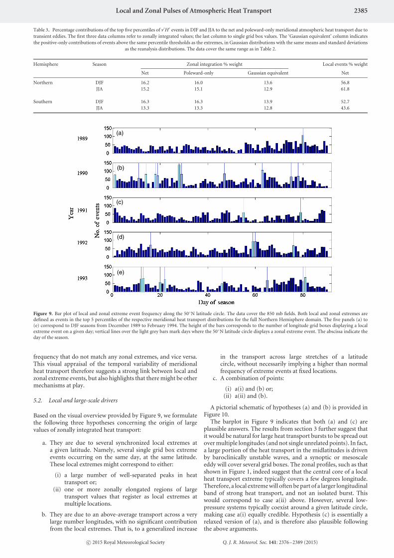
Local and Zonal Pulses of Atmospheric Heat Transport 2385
Table 3. Percentage contributions of the top five percentiles of v′H′ events in DJF and JJA to the net and poleward-only meridional atmospheric heat transport due totransient eddies. The first three data columns refer to zonally integrated values; the last column to single grid box values. The ‘Gaussian equivalent’ column indicatesthe positive-only contributions of events above the same percentile thresholds as the extremes, in Gaussian distributions with the same means and standard deviations
as the reanalysis distributions. The data cover the same range as in Table 2.
Hemisphere Season Zonal integration % weight Local events % weight
Net Poleward-only Gaussian equivalent Net
Northern DJF 16.2 16.0 13.6 56.8JJA 15.2 15.1 12.9 61.8
Southern DJF 16.3 16.3 13.9 52.7JJA 13.3 13.3 12.8 43.6
(b)
(a)
(d)
(e)
(c)
Figure 9. Bar plot of local and zonal extreme event frequency along the 50◦N latitude circle. The data cover the 850 mb fields. Both local and zonal extremes aredefined as events in the top 5 percentiles of the respective meridional heat transport distributions for the full Northern Hemisphere domain. The five panels (a) to(e) correspond to DJF seasons from December 1989 to February 1994. The height of the bars corresponds to the number of longitude grid boxes displaying a localextreme event on a given day; vertical lines over the light grey bars mark days where the 50◦N latitude circle displays a zonal extreme event. The abscissa indicate theday of the season.
frequency that do not match any zonal extremes, and vice versa.This visual appraisal of the temporal variability of meridionalheat transport therefore suggests a strong link between local andzonal extreme events, but also highlights that there might be othermechanisms at play.
5.2. Local and large-scale drivers
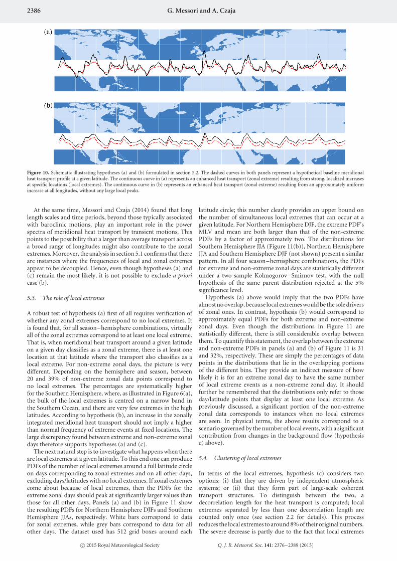
Based on the visual overview provided by Figure 9, we formulatethe following three hypotheses concerning the origin of largevalues of zonally integrated heat transport:
a. They are due to several synchronized local extremes ata given latitude. Namely, several single grid box extremeevents occurring on the same day, at the same latitude.These local extremes might correspond to either:
(i) a large number of well-separated peaks in heattransport or;
(ii) one or more zonally elongated regions of largetransport values that register as local extremes atmultiple locations.
b. They are due to an above-average transport across a verylarge number longitudes, with no significant contributionfrom the local extremes. That is, to a generalized increase
in the transport across large stretches of a latitudecircle, without necessarily implying a higher than normalfrequency of extreme events at fixed locations.
c. A combination of points:
(i) a(i) and (b) or;(ii) a(ii) and (b).
A pictorial schematic of hypotheses (a) and (b) is provided inFigure 10.
The barplot in Figure 9 indicates that both (a) and (c) areplausible answers. The results from section 3 further suggest thatit would be natural for large heat transport bursts to be spread outover multiple longitudes (and not single unrelated points). In fact,a large portion of the heat transport in the midlatitudes is drivenby baroclinically unstable waves, and a synoptic or mesoscaleeddy will cover several grid boxes. The zonal profiles, such as thatshown in Figure 1, indeed suggest that the central core of a localheat transport extreme typically covers a few degrees longitude.Therefore, a local extreme will often be part of a larger longitudinalband of strong heat transport, and not an isolated burst. Thiswould correspond to case a(ii) above. However, several low-pressure systems typically coexist around a given latitude circle,making case a(i) equally credible. Hypothesis (c) is essentially arelaxed version of (a), and is therefore also plausible followingthe above arguments.
c© 2015 Royal Meteorological Society Q. J. R. Meteorol. Soc. 141: 2376–2389 (2015)
2386 G. Messori and A. Czaja
Figure 10. Schematic illustrating hypotheses (a) and (b) formulated in section 5.2. The dashed curves in both panels represent a hypothetical baseline meridionalheat transport profile at a given latitude. The continuous curve in (a) represents an enhanced heat transport (zonal extreme) resulting from strong, localized increasesat specific locations (local extremes). The continuous curve in (b) represents an enhanced heat transport (zonal extreme) resulting from an approximately uniformincrease at all longitudes, without any large local peaks.
At the same time, Messori and Czaja (2014) found that longlength scales and time periods, beyond those typically associatedwith baroclinic motions, play an important role in the powerspectra of meridional heat transport by transient motions. Thispoints to the possibility that a larger than average transport acrossa broad range of longitudes might also contribute to the zonalextremes. Moreover, the analysis in section 5.1 confirms that thereare instances where the frequencies of local and zonal extremesappear to be decoupled. Hence, even though hypotheses (a) and(c) remain the most likely, it is not possible to exclude a prioricase (b).
5.3. The role of local extremes
A robust test of hypothesis (a) first of all requires verification ofwhether any zonal extremes correspond to no local extremes. Itis found that, for all season–hemisphere combinations, virtuallyall of the zonal extremes correspond to at least one local extreme.That is, when meridional heat transport around a given latitudeon a given day classifies as a zonal extreme, there is at least onelocation at that latitude where the transport also classifies as alocal extreme. For non-extreme zonal days, the picture is verydifferent. Depending on the hemisphere and season, between20 and 39% of non-extreme zonal data points correspond tono local extremes. The percentages are systematically higherfor the Southern Hemisphere, where, as illustrated in Figure 6(a),the bulk of the local extremes is centred on a narrow band inthe Southern Ocean, and there are very few extremes in the highlatitudes. According to hypothesis (b), an increase in the zonallyintegrated meridional heat transport should not imply a higherthan normal frequency of extreme events at fixed locations. Thelarge discrepancy found between extreme and non-extreme zonaldays therefore supports hypotheses (a) and (c).
The next natural step is to investigate what happens when thereare local extremes at a given latitude. To this end one can producePDFs of the number of local extremes around a full latitude circleon days corresponding to zonal extremes and on all other days,excluding days/latitudes with no local extremes. If zonal extremescome about because of local extremes, then the PDFs for theextreme zonal days should peak at significantly larger values thanthose for all other days. Panels (a) and (b) in Figure 11 showthe resulting PDFs for Northern Hemisphere DJFs and SouthernHemisphere JJAs, respectively. White bars correspond to datafor zonal extremes, while grey bars correspond to data for allother days. The dataset used has 512 grid boxes around each
latitude circle; this number clearly provides an upper bound onthe number of simultaneous local extremes that can occur at agiven latitude. For Northern Hemisphere DJF, the extreme PDF’sMLV and mean are both larger than that of the non-extremePDFs by a factor of approximately two. The distributions forSouthern Hemisphere JJA (Figure 11(b)), Northern HemisphereJJA and Southern Hemisphere DJF (not shown) present a similarpattern. In all four season–hemisphere combinations, the PDFsfor extreme and non-extreme zonal days are statistically differentunder a two-sample Kolmogorov–Smirnov test, with the nullhypothesis of the same parent distribution rejected at the 5%significance level.
Hypothesis (a) above would imply that the two PDFs havealmost no overlap, because local extremes would be the sole driversof zonal ones. In contrast, hypothesis (b) would correspond toapproximately equal PDFs for both extreme and non-extremezonal days. Even though the distributions in Figure 11 arestatistically different, there is still considerable overlap betweenthem. To quantify this statement, the overlap between the extremeand non-extreme PDFs in panels (a) and (b) of Figure 11 is 31and 32%, respectively. These are simply the percentages of datapoints in the distributions that lie in the overlapping portionsof the different bins. They provide an indirect measure of howlikely it is for an extreme zonal day to have the same numberof local extreme events as a non-extreme zonal day. It shouldfurther be remembered that the distributions only refer to thoseday/latitude points that display at least one local extreme. Aspreviously discussed, a significant portion of the non-extremezonal data corresponds to instances when no local extremesare seen. In physical terms, the above results correspond to ascenario governed by the number of local events, with a significantcontribution from changes in the background flow (hypothesisc) above).
5.4. Clustering of local extremes
In terms of the local extremes, hypothesis (c) considers twooptions: (i) that they are driven by independent atmosphericsystems; or (ii) that they form part of large-scale coherenttransport structures. To distinguish between the two, adecorrelation length for the heat transport is computed; localextremes separated by less than one decorrelation length arecounted only once (see section 2.2 for details). This processreduces the local extremes to around 8% of their original numbers.The severe decrease is partly due to the fact that local extremes
c© 2015 Royal Meteorological Society Q. J. R. Meteorol. Soc. 141: 2376–2389 (2015)

Local and Zonal Pulses of Atmospheric Heat Transport 2387
Figure 11. The PDFs of the number of local extreme events around a full latitude circle for days that are in the top 5% (white) and days that are in the bottom95% (grey) of the distributions of the zonally integrated meridional atmospheric heat transport due to transient eddies. The PDFs cover (a,c) Northern HemisphereDJF and (b,d) Southern Hemisphere JJA data, over the same temporal and spatial range as Figure 7. (a) and (b) consider all local extremes; (c) and (d) only countwell-separated local extremes. Only days/latitudes with at least one local extreme are considered. The most likely values are respectively (a) 60 (extremes, in white) and28 (non-extremes, in grey), (b) 68 and 20, (c) 4 and 1 and (d) 5 and 2. The corresponding means are respectively (a) 64 and 31, (b) 70 and 33, (c) 4.0 and 2.3 and(d) 5.2 and 2.9. The vertical lines show the bins corresponding to the most likely values.
extend across several grid boxes, as seen in section 3. A singlelocal maximum will therefore be counted multiple times if theselection is purely based on the exceedance of a threshold. Therest of the decrease can be ascribed to multiple closely spacedlocal extreme peaks which form part of a single, extensive bandof strong meridional heat transport, and are counted only once.The local extremes therefore present a pronounced clustering,corresponding to hypothesis c(ii). This is in agreement with thewell-defined geographical regions of high extreme event frequencyshown in Figure 6(a).
The fact that clusters of local extremes exist, however, doesnot necessarily mean that they actively drive the zonal extremes.Indeed, the clustering might be a general property of the local heattransport, and be completely unrelated to the zonal extremes.We therefore test whether there is any systematic relationshipbetween the additional heat transport seen on extreme zonal daysand the size and/or number of clusters of local extremes. To dothis, the PDF analysis described in section 5.3 above is repeatedfor the new set of well-separated local extremes. Panels (c) and(d) in Figure 11 display the results for Northern HemisphereDJF and Southern Hemisphere JJA, respectively. As before, the
extreme zonal days display systematically more local extremesthan the non-extreme zonal days. The distributions are againstatistically different under a two-sample Kolmogorov–Smirnovtest, at the 95% confidence level, for all hemispheres and seasons.However, it is immediately noticeable that the overlap betweenthe distributions for the extreme and non-extreme zonal days ismuch larger than before. The overlaps are now 55% for NorthernHemisphere DJF (panel (c)) and 46% for Southern HemisphereJJA (panel (d)). If the additional heat transport during extremezonal days was entirely due to larger clusters of local events, thetwo PDFs in each of the panels would overlap completely. Infact, each cluster would be counted only once, regardless of thenumber of local extremes forming it. The opposite would occur ifthe additional transport were exclusively due to a larger numberof clusters.
5.5. The weak synchronisation hypothesis
The picture that emerges from the above analysis correspondsto a zonally integrated heat transport that is largely, but not
c© 2015 Royal Meteorological Society Q. J. R. Meteorol. Soc. 141: 2376–2389 (2015)

2388 G. Messori and A. Czaja
exclusively, governed by the number of local extreme events. Itis further found that the local extremes driving the transporttend to cluster in zonally elongated bands. This corresponds tohypothesis c(ii) of the original list. If local extremes forming partof the same cluster are counted only once, approximately halfthe extreme zonal days have the same number of clusters as thenon-extreme ones. This indicates that a zonal extreme may comeabout because of either more frequent or larger clusters of localextremes (or indeed both).
We therefore conclude that the zonal heat transport ischaracterized by a weak synchronization effect, whereby zonalextremes are partly driven by synchronized, zonally elongatedbands of local extremes. However, the zonal extremes have amuch weaker impact on the overall transport distribution thantheir single-point counterparts, as shown in section 4.3.
Finally, it should be noted that there is a caveat to themethodology adopted here. The validity of the hypotheses madeabove may depend on the exact definition of local extremes interms of percentiles of a distribution. Indeed, if the percentilethreshold were to be changed by tens of percentiles, the picturewould in turn change. However, the circulation maps shownin section 3 are specific to only the strongest transport events,suggesting that data points above the 95th percentile are physicallydifferent from the norm. This threshold is therefore a suitableselection criterion. Although it could be argued that the 93rdor 97th percentiles would be equally valid choices, it wouldbe unphysical to choose, for example, the 70th percentile asthreshold. Moreover, if the percentiles defining local extremeschange, so do those defining the zonal ones. For example, if thelocal extremes were to be defined as events within the top 10percentiles of the single-point distribution, the same definitionwould then be applied to the zonally integrated distribution inorder to select the extreme zonal days. This definition is a limitcase because, as discussed in section 3, the events selected by thisrelaxed criterion lack some of the circulation features seen inFigure 1. If such a threshold were adopted, the fractional overlapof the PDFs corresponding to those in Figure 11(a) and (b)would rise from 31 and 32% to 64 and 51% respectively, but thedistributions for extreme and non-extreme days would remainstatistically different. We therefore conclude that large changes inthe chosen extreme event threshold would not be justifiable froma dynamics standpoint, while small changes do not significantlyalter the findings discussed here.
6. Further discussion and conclusions
The present article examines zonally integrated meridionalatmospheric heat transport due to transient eddies, focusingon low levels in the mid- and high latitudes. Previous studieshave already shown that the local transport is very discontinuousin nature, and is very sensitive to a few extreme events everyseason (e.g., Swanson and Pierrehumbert, 1997; MC13; Messoriand Czaja, 2014). Here, it is shown that the local extremes canbe associated with precise circulation features. In the storm-trackregions, these correspond primarily to WCB-type structures.Different circulation patterns, such as cold air outbreaks, emergein other regions.
The existence of these circulation analogues for local extremessuggests that there might be a measure of synchronization betweenextremes at different longitudes, hence giving rise to large valuesof zonally integrated meridional transport, or zonal extremes.This is indeed seen to be the case: the zonal extremes in theERA-Interim data are found to be partly due to numerous localextremes occurring simultaneously around a given latitude circle.The local extremes tend to cluster in zonally elongated bands,with a more pronounced clustering during extreme zonal days. Inaddition to this, the zonal events also display a contribution fromincreased transport at non-extreme locations. These two featuressuggest that scales larger than those associated with the extremesact to enhance the transport over wide areas of the latitude circle.
Such inference is in agreement with the results of Messori andCzaja (2014), who found that long length scales (zonal wavenumbers ≤ 4) and time periods (periods >8 days), beyond thosetypically associated with baroclinic motions, play an importantrole in the power spectra of meridional heat transport by transienteddies.
The percentage contributions of zonal extreme events to thenet, zonally integrated meridional heat transport are significantlylower than the corresponding values found for local extremes(MC13). They are still, however, significantly larger than thosefound for Gaussian distributions with the same means andstandard deviations as the transport PDFs.
It should also be remembered that the local poleward transportextremes are often associated with a return equatorward transport(see Figure 1). Such return transport is highly variable, and mightprovide an additional explanation as to why days with a large num-ber of local extremes do not always correspond to zonal extremes.As shown in Figure 11, a small fraction of non-extreme zonal daysdisplays a very large number of local extremes – larger, in fact,than the most likely value for an extreme zonal day. A realistichypothesis is that these outlying non-extreme days are character-ized by local extremes that have uncommonly strong recirculationfeatures, such that their net transport is smaller than usual.
Extending the analysis of recirculation features to a global scaleit is interesting to note that, even when considering zonally inte-grated values, the transport is not always polewards. In fact, the850 mb zonally integrated transport is negative on a small fractionof the days and latitudes considered. Only a very brief analysis ofthese events has been performed here. The results suggest that thenegative transport is primarily driven by the large-scale motions,associated with time-scales beyond 8 days. This is consistent withthe picture of baroclinic-scale growing systems (periods <8 days)mainly accounting for poleward transport values, and the weakeror even negative values corresponding to decaying waves. It is fur-ther found that the transport by transient motions displays a highvertical coherence, meaning that when the transport at 850 mb isnegative, the transport at upper levels has a significant chance ofalso being negative. When the net atmospheric energy transport iscomputed, the other components of the transport (e.g., climato-logical stationary eddies and/or compensation by a reduced Ferrelcell) often balance out the negative contribution by transientmotions. However, there is a small fraction of cases (1–2% ofthe total) where a negative 850 mb transport corresponds to anegative net transport. On these days, at a given latitude, theatmosphere carries energy towards the Equator. A more in-depthanalysis, based on existing studies of the co-variability of thedifferent components of the atmospheric energy transport (e.g.,Trenberth and Stepaniak, 2003), would be required in order todetermine the dynamical drivers of these events.
Although the general picture seems coherent, there are someaspects that require further clarification. The first is whether therole of the longer time-scales and length scales, mentioned above,is compatible with a direct correspondence between the extremesand the local atmospheric features discussed in section 3. Thedefinition of ‘extreme’ adopted here is based on a numericalthreshold. When considering the spectral features of the heattransport, large variations in power at scales consistent with baro-clinic motions could be sufficient to determine whether eventswith high power at larger scales classify as extremes or not. Thatis, the power in a specific region of the spectrum could determinewhether a given event falls above or below the threshold, eventhough the said region might not account for the majority of thenet spectral power. One can therefore reconcile the spectral andsynoptic analyses, and interpret the extreme events as regionallycoherent synoptic features superimposed on planetary-scalevariability. This view is further strengthened by the fact that theclustering of local extremes is enhanced during zonal extremedays. In fact, the formation of the clusters could be facilitated byan enhanced heat transport driven by planetary-scale modes.
In this regard a detailed spectral analysis, studying thecontributions of the different periods to the vertical and zonal
c© 2015 Royal Meteorological Society Q. J. R. Meteorol. Soc. 141: 2376–2389 (2015)
Local and Zonal Pulses of Atmospheric Heat Transport 2389
structure of the extremes, could prove valuable. Applying a high-pass or band-pass filter to the data, with an upper cut-off around6–8 days, would remove the planetary-scale component andhighlight the structure of the local synoptic motions.
A second point concerns the differences seen in the zonallyintegrated transport distributions of the two hemispheres. Ithas been suggested in section 4 that the bimodality seen in theSouthern Hemisphere distribution is the result of two distinctpatterns. One holds for the lower latitudes, where there are largervalues of zonally integrated transport. The other holds for thehigher latitudes, where the zonally integrated transport is smaller.Although, in general, this is also true of the Northern Hemisphere,the two hemispheres display a clear difference in the geographicaldistributions of the local extremes. In the Northern Hemisphere,the location of the extreme events is varied, with the two stormtracks playing an important role, but with several other areas ofvigorous activity at higher latitudes (MC13). This is in contrast tothe Southern Hemisphere, where the vast majority of the extremeevents is concentrated in a narrow latitudinal band, providing amuch sharper contrast between the lower and higher latitudes(see Figure 6(b)).
Regardless of these differences, both hemispheres display apronounced variability on a zonally integrated level, whichtranslates into the existence of zonally integrated transportextremes. This is very significant for the energy balance of thehigh latitudes. The past decade has seen an unprecedented sea-ice loss in the Arctic basin, which has been underestimated byalmost all climate models (e.g., Stroeve et al., 2007). There arestudies suggesting that anomalous atmospheric heat transportconvergence at the high latitudes might drive a local long-waveforcing, playing a significant role in the melt process (Graversenet al., 2011). Further efforts in understanding and modellingthe variability of zonally integrated meridional heat transport,coupled with a study of the possible impacts of climate changeon such variability, would therefore be crucial in order to betterunderstand the future of the polar regions.
Acknowledgements
During the research, G. Messori has been funded by the UK’sNatural Environment Research Council, as part of the RAPID-RAPIT project, and by Sweden’s Vetenskapsradet, as part ofthe MILEX project. ERA-Interim reanalysis data were obtainedfrom the BADC FTP server at ftp.badc.rl.ac.uk. We thank theanonymous reviewers for the many helpful comments; we alsothank C. H. O’Reilly for his suggestions and for editing the article.Finally, we are very grateful to R. G. Graversen for providingthe vertically integrated heat transport data and for a stimulatingdiscussion on equatorward transport events.
Supporting information
The following supporting information is available as part of theonline article:
File S1. The role of velocity and MSE in driving heat transportextremes.
File S2. Time-filtered heat transport.
References
Ambaum MHP, Novak L. 2014. A nonlinear oscillator describing stormtrack variability. Q. J. R. Meteorol. Soc. 140: 2680–2684, doi: 10.1002/qj.2352.
Boutle I, Belcher S, Plant R. 2010. Moisture transport in mid-latitude cyclones.Q. J. R. Meteorol. Soc. 136: 1–14.
Browning KA. 1997. The dry intrusion perspective of extra-tropical cyclonedevelopment. Meteorol. Appl. 4: 317–324.
Catto J, Shaffrey L, Hodges K. 2010. Can climate models capture the structureof extratropical cyclones? J. Clim. 23: 1621–1635.
Chang EKM. 1993. Downstream development of baroclinic waves as inferredfrom regression analysis. J. Atmos. Sci. 50: 2038–2053.
Donohoe A, Battisti DS. 2012. What determines meridional heat transport inclimate models? J. Clim. 25: 3832–3850.
Eckhardt S, Stohl A, Wernli H, James P, Forster C, Spichtinger N. 2004. A15-year climatology of warm conveyor belts. J. Clim. 17: 218–237.
Graversen RG. 2006. Do changes in the mid-latitude circulation haveany impact on the Arctic surface air temperature trend? J. Clim. 19:5422–5438.
Graversen RG, Mauritsen T, Drijfhout S, Tjernstrom M, Martensson S. 2011.Warm winds from the Pacific caused extensive Arctic sea-ice melt in summer2007. Clim. Dyn. 36: 2103–2112.
Hwang Y-T, Frierson DMW. 2010. Increasing atmospheric poleward energytransport with global warming. Geophys. Res. Lett. 37: L24807, doi:10.1029/2010GL045440.
Kolstad EW, Bracegirdle TJ. 2008. Marine cold-air outbreaks in the future: Anassessment of IPCC AR4 model results for the Northern Hemisphere. Clim.Dyn. 30: 871–885.
Lau N-C. 1978. On the three-dimensional structure of the observed transienteddy statistics of the Northern Hemisphere wintertime circulation. J. Atmos.Sci. 35: 1900–1923.
Madonna E, Wernli H, Joos H, Martius O. 2014. Warm conveyor beltsin the ERA-interim dataset (1979–2010). Part I: Climatology andpotential vorticity evolution. J. Clim. 27: 3–26, doi: 10.1175/JCLI-D-12-00720.1.
Messori G, Czaja A. 2013. On the sporadic nature of meridional heattransport by transient eddies. Q. J. R. Meteorol. Soc. 139: 999–1008,doi: 10.1002/qj.2011.
Messori G, Czaja A. 2014. Some considerations on the spectral features ofmeridional heat transport by transient eddies. Q. J. R. Meteorol. Soc. 140:1377–1386, doi: 10.1002/qj.2224.
Nakamura H, Izumi T, Sampe T. 2002. Interannual and decadal modulationsrecently observed in the Pacific storm track activity and East Asian WinterMonsoon. J. Clim. 15: 1855–1874.
Neelin JD, Held IM. 1987. Modelling tropical convergence based on the moiststatic energy budget. Mon. Weather Rev. 115: 3–12.
Peixoto J, Oort A. 1992. Physics of Climate. American Institute of Physics NewYork, NY.
Pinto JG, Gomara I, Masato G, Dacre HF, Woollings T, Caballero R. 2014.Large-Scale dynamics associated with clustering of extra-tropical cyclonesaffecting Western Europe. J. Geophys. Res. Atmos. 119: 13704–13719, doi:10.1002/2014JD022305.
Simmons A, Uppala S, Dee D, Kobayashi S. 2006. ERA-Interim: New ECMWFreanalysis products from 1989 onwards. ECMWF Newsl. 110: 25–35.
Stroeve J, Holland MM, Meier W, Scambos T, Serreze M. 2007. Arcticsea ice decline: Faster than forecast. Geophys. Res. Lett. 34: L09501, doi:10.1029/2007GL029703.
Swanson KL, Pierrehumbert RT. 1997. Lower-tropospheric heat transport inthe Pacific storm track. J. Atmos. Sci. 54: 1533–1543.
Trenberth KE. 1991. Climate diagnostics from global analyses: Conservationof mass in ECMWF analyses. J. Clim. 4: 707–722.
Trenberth KE, Stepaniak DP. 2003. Covariability of components ofpoleward atmospheric energy transports on seasonal and interannualtimescales. J. Clim. 16: 3691–3705, doi: 10.1175/1520-0442(2003)016<3691:COCOPA>2.0.CO;2.
Zelinka MD, Hartmann DL. 2012. Climate feedbacks and their implications forpoleward energy flux changes in a warming climate. J. Clim. 25: 608–624,doi: 10.1175/JCLI-D-11-00096.1.
c© 2015 Royal Meteorological Society Q. J. R. Meteorol. Soc. 141: 2376–2389 (2015)