on modeling and analyzing cost factors in information...

On Modeling and Analyzing Cost Factorsin Information Systems Engineering

Bela Mutschler1,2 and Manfred Reichert2,3

1 Daimler AG, Group Research, P.O. Box 2360, 89013 Ulm, [email protected]

2 Information Systems Group, University of Twente, The [email protected]

3 Institute of Databases and Information Systems, University of Ulm, [email protected]

Abstract. Introducing enterprise information systems (EIS) is usually associatedwith high costs. It is therefore crucial to understand those factors that determine orinfluence these costs. Though software cost estimation has received considerableattention during the last decades, it is difficult to apply existing approaches to EIS.This difficulty particularly stems from the inability of these methods to deal withthe dynamic interactions of the many technological, organizational and project-driven cost factors which specifically arise in the context of EIS. Picking up thisproblem, we introduce the EcoPOST framework to investigate the complex coststructures of EIS engineering projects through qualitative cost evaluation models.This paper extends previously described concepts and introduces design rulesand guidelines for cost evaluation models in order to enhance the development ofmeaningful and useful EcoPOST cost evaluation models. A case study illustratesthe benefits of our approach. Most important, our EcoPOST framework is animportant tool supporting EIS engineers in gaining a better understanding of thecritical factors determining the costs of EIS engineering projects.

Keywords: Information Systems Engineering, Cost Analysis, Evaluation Mod-els, Simulation.

1 Introduction

While the benefits of enterprise information systems (EIS) are usually justified by im-proved process performance [1], there exist no approaches for systematically analyz-ing related cost factors and their dependencies. Though software cost estimation hasreceived considerable attention during the last decades [2] and has become an essen-tial task in information systems engineering, it is difficult to apply existing approachesto EIS, particularly if the considered EIS shall provide active business process sup-port. This difficulty stems from the inability of these approaches to cope with thenumerous technological, organizational and project-driven cost factors which have tobe considered in the context of process-aware EIS (and which do only partly exist indata- or function-centered information systems) [3]. As an example consider the signif-icant costs for redesigning business processes. Another challenge deals with the manydependencies existing between different cost factors. Activities for business process

Z. Bellahsene and M. Leonard (Eds.): CAiSE 2008, LNCS 5074, pp. 510–524, 2008.c© Springer-Verlag Berlin Heidelberg 2008

On Modeling and Analyzing Cost Factors in Information Systems Engineering 511

redesign, for example, can be influenced by intangible impact factors like availableprocess knowledge or end user fears. These dependencies, in turn, result in dynamic ef-fects which influence the overall costs of EIS engineering projects. Existing evaluationtechniques [4] are typically unable to deal with such dynamic effects as they rely on toostatic models based upon snapshots of the considered software system.

What is needed is an approach that enables project managers and EIS engineers tomodel and investigate the complex interplay between the many cost and impact fac-tors that arise in the context of EIS. This paper presents the EcoPOST methodology,a sophisticated and practically validated, model-based methodology to better under-stand and systematically investigate the complex cost structures of EIS engineeringprojects. Specifically, this paper extends our previous work on EcoPOST [5] by intro-ducing model design rules and modeling guidelines, which enhance the development ofmeaningful and useful evaluation models.

Section 2 summarizes the EcoPOST methodology. Section 3 introduces rules fordesigning evaluation models and Section 4 describes modeling guidelines. Section 5summarizes results from one of our case studies in order to illustrate the benefits ofthe EcoPOST approach. It further discusses issues related to validation research from amore general perspective. Section 6 concludes with a summary.

2 The EcoPOST Cost Analysis Methodology

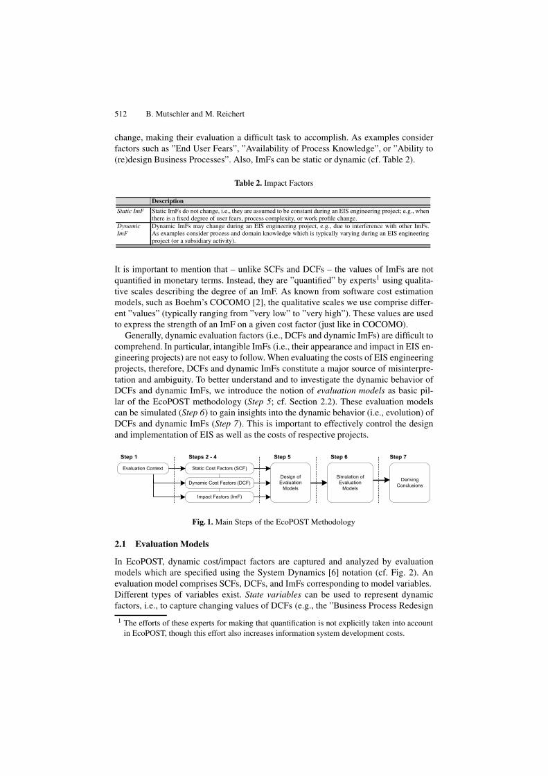
Our EcoPOST methodology was designed to ease the realization of process-aware EISin the automotive industry (and was, consequently, also validated and piloted in severalEIS engineering projects in this domain). The EcoPOST methodology comprises sevensteps (cf. Fig. 1). Step 1 concerns the comprehension of an evaluation scenario. Thisis crucial for developing problem-specific evaluation models. The following two steps(Steps 2 and 3) deal with the identification of two different kinds of Cost Factors repre-senting costs that can be quantified in terms of money (cf. Table 1): Static Cost Factors(SCFs) and Dynamic Cost Factors (DCFs).

Step 4 deals with the identification of Impact Factors (ImFs), i.e., intangible factorsthat influence DCFs and other ImFs. We distinguish between organizational, project-specific, and technological ImFs. ImFs cause the value of DCFs (and other ImFs) to

Table 1. Cost Factors

Description

SCF Static Cost Factors (SCFs) represent costs whose values do not change during an EIS engineering project (exceptfor their time value, which is not further considered in the following). Typical examples: software license costs,hardware costs and costs for external consultants.

DCF Dynamic Cost Factors (DCFs), in turn, represent costs that are determined by activities related to an EIS engineer-ing project. The (re)design of business processes prior to the introduction of EIS, for example, constitutes such anactivity. As another example consider the performance of interview-based process analysis. These activities causemeasurable efforts which, in turn, vary due to the influence of intangible impact factors. The DCF ”Costs for Busi-ness Process Redesign” may be influenced, for instance, by an intangible factor ”Willingness of Staff Membersto Support Process (Re)Design Activities”. Obviously, if staff members do not contribute to a (re)design projectby providing needed information (e.g., about process details), any redesign effort will be ineffective and result inincreasing (re)design costs. If staff willingness is additionally varying during the (re)design activity (e.g., due to achanging communication policy), the DCF will be subject to even more complex effects. In the EcoPOST frame-work, intangible factors like the one described are represented by impact factors.

512 B. Mutschler and M. Reichert

change, making their evaluation a difficult task to accomplish. As examples considerfactors such as ”End User Fears”, ”Availability of Process Knowledge”, or ”Ability to(re)design Business Processes”. Also, ImFs can be static or dynamic (cf. Table 2).

Table 2. Impact Factors

Description

Static ImF Static ImFs do not change, i.e., they are assumed to be constant during an EIS engineering project; e.g., whenthere is a fixed degree of user fears, process complexity, or work profile change.

DynamicImF

Dynamic ImFs may change during an EIS engineering project, e.g., due to interference with other ImFs.As examples consider process and domain knowledge which is typically varying during an EIS engineeringproject (or a subsidiary activity).

It is important to mention that – unlike SCFs and DCFs – the values of ImFs are notquantified in monetary terms. Instead, they are ”quantified” by experts1 using qualita-tive scales describing the degree of an ImF. As known from software cost estimationmodels, such as Boehm’s COCOMO [2], the qualitative scales we use comprise differ-ent ”values” (typically ranging from ”very low” to ”very high”). These values are usedto express the strength of an ImF on a given cost factor (just like in COCOMO).

Generally, dynamic evaluation factors (i.e., DCFs and dynamic ImFs) are difficult tocomprehend. In particular, intangible ImFs (i.e., their appearance and impact in EIS en-gineering projects) are not easy to follow. When evaluating the costs of EIS engineeringprojects, therefore, DCFs and dynamic ImFs constitute a major source of misinterpre-tation and ambiguity. To better understand and to investigate the dynamic behavior ofDCFs and dynamic ImFs, we introduce the notion of evaluation models as basic pil-lar of the EcoPOST methodology (Step 5; cf. Section 2.2). These evaluation modelscan be simulated (Step 6) to gain insights into the dynamic behavior (i.e., evolution) ofDCFs and dynamic ImFs (Step 7). This is important to effectively control the designand implementation of EIS as well as the costs of respective projects.

Impact Factors (ImF)

Dynamic Cost Factors (DCF)

Static Cost Factors (SCF)

Steps 2 - 4 Step 5 Step 6

Design ofEvaluation

Models

Step 1 Step 7

DerivingConclusions

Simulation ofEvaluation

Models

Evaluation Context

Fig. 1. Main Steps of the EcoPOST Methodology

2.1 Evaluation Models

In EcoPOST, dynamic cost/impact factors are captured and analyzed by evaluationmodels which are specified using the System Dynamics [6] notation (cf. Fig. 2). Anevaluation model comprises SCFs, DCFs, and ImFs corresponding to model variables.Different types of variables exist. State variables can be used to represent dynamicfactors, i.e., to capture changing values of DCFs (e.g., the ”Business Process Redesign

1 The efforts of these experts for making that quantification is not explicitly taken into accountin EcoPOST, though this effort also increases information system development costs.


Costs”; cf. Fig. 2A) and dynamic ImFs (e.g., ”Process Knowledge”). A state variableis graphically denoted as rectangle (cf. Fig. 2A), and its value at time t is determinedby the accumulated changes of this variable from starting point t0 to present moment t(t > t0); similar to a bathtub which accumulates – at a defined moment t – the amountof water poured into it in the past. Typically, state variables are connected to at leastone source or sink which are graphically denoted as cloud-like symbols (except forstate variables connected to other ones) (cf. Fig. 2A). Values of state variables changethrough inflows and outflows. Graphically, both flow types are depicted by twin-arrowswhich either point to (in the case of an inflow) or out of (in the case of an outflow) thestate variable (cf. Fig. 2A). Picking up again the bathtub image, an inflow is a pipe thatadds water to the bathtub, i.e., inflows increase the value of state variables. An outflow,by contrast, is a pipe that purges water from the bathtub, i.e., outflows decrease thevalue of state variables. The DCF ”Business Process Redesign Costs” shown in Fig.2A, for example, increases through its inflow (”Cost Increase”) and decreases throughits outflow (”Cost Decrease”). Returning to the bathtub image, we further need ”watertaps” to control the amount of water flowing into the bathtub, and ”drains” to specify theamount of water flowing out. For this purpose, a rate variable is assigned to each flow(graphically depicted by a valve; cf. Fig. 2A). In particular, a rate variable controls theinflow/outflow it is assigned to based on those SCFs, DCFs, and ImFs which influenceit. It can be considered as an interface which is able to merge SCFs, DCFs, and ImFs.

A) State Variables & Flows

Costs

BusinessProcess

Redesign

Controlsthe Inflow

Controlsthe Outflow

DCF

CostIncrease

CostDecrease

Auxiliary Variables

Rate Variables

Dynamic Cost Factors Sources and Sinks

Dynamic Impact Factors

Text

Static Cost Factor [Text]

Static Impact Factor (Text)

B) Auxiliary Variables

Cost Increase Cost Decrease

AdjustedProcess Analysis

Costs

-

-

+

Analysis Costsper Week]+

WaterTap

WaterDrain

[SCF1]

[SCF2]

(ImFS)

AuxiliaryVariable

++

--

Business ProcessRedesign Costs

Ability to RedesignBusiness

Processes

[Planned

Notation:Flows

Links [+|-]

ProcessKnowledge

DomainKnowledge

Fig. 2. Evaluation Model Notation and initial Examples

Besides state variables, evaluation models may comprise constants and auxiliaryvariables. Constants are used to represent static evaluation factors, i.e., SCFs and staticImFs. Auxiliary variables, in turn, represent intermediate variables and typically bringtogether – like rate variables – cost and impact factors, i.e., they merge SCFs, DCFs,and ImFs. As an example consider the auxiliary variable ”Adjusted Process AnalysisCosts” in Fig. 2B, which merges the three dynamic ImFs ”Process Knowledge”, ”Do-main Knowledge”, and ”Ability to Redesign Business Processes” and the SCF ”PlannedAnalysis Costs per Week”. Both constants and auxiliary variables are integrated into anevaluation model with links (not flows), i.e., labeled arrows. A positive link (labeled


with ”+”) between x and y (with y as dependent variable) indicates that y will tend inthe same direction if a change occurs in x. A negative link (labeled with ”-”) expressesthat the dependent variable y will tend in the opposite direction if the value of x changes.Altogether, we define:

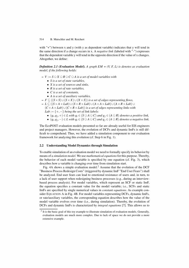
Definition 2.1 (Evaluation Model). A graph EM = (V, F, L) is denotes as evaluationmodel, if the following holds:

– V := S ∪ X ∪ R ∪ C ∪ A is a set of model variables with• S is a set of state variables,• X is a set of sources and sinks,• R is a set of rate variables,• C is a set of constants,• A is a set of auxiliary variables,

– F ⊆ ((S × S)∪ (S × X)∪ (X × S)) is a set of edges representing flows,– L ⊆ ((S × A × Lab)∪ (S × R × Lab)∪ (A×A×Lab)∪ (A ×R×Lab) ∪

(C × A × Lab)∪ (C× R × Lab)) is a set of edges representing links withLab := {+,−} being the set of link labels:

• (qi,q j,+) ∈ L with qi ∈ (S ∪ A ∪ C) and q j ∈ (A ∪ R) denotes a positive link,• (qi,q j,−) ∈ L with qi ∈ (S ∪ A ∪ C) and q j ∈ (A ∪ R) denotes a negative link.

The EcoPOST evaluation models presented so far are already useful for EIS engineersand project managers. However, the evolution of DCFs and dynamic ImFs is still dif-ficult to comprehend. Thus, we have added a simulation component to our evaluationframework for analyzing this evolution (cf. Step 6 in Fig. 1).

2.2 Understanding Model Dynamics through Simulation

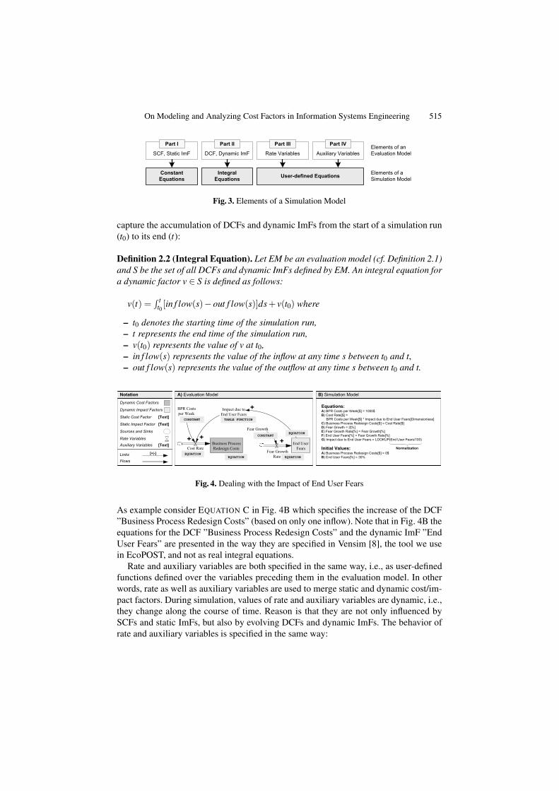
To enable simulation of an evaluation model we need to formally specify its behavior bymeans of a simulation model. We use mathematical equations for this purpose. Thereby,the behavior of each model variable is specified by one equation (cf. Fig. 3), whichdescribes how a variable is changing over time from simulation start.

Fig. 4A shows a simple evaluation model.2 Assume that the evolution of the DCF”Business Process Redesign Costs” (triggered by dynamic ImF ”End User Fears”) shallbe analyzed. End user fears can lead to emotional resistance of users and, in turn, toa lack of user support when redesigning business processes (e.g., during an interview-based process analysis). For model variables, which represent an SCF or static ImF,the equation specifies a constant value for the model variable; i.e., SCFs and staticImFs are specified by single numerical values in constant equations. As example con-sider EQUATION A in Fig. 4B. For model variables representing DCFs, dynamic ImFs,or rate/auxiliary variables, the corresponding equation describes how the value of themodel variable evolves over time (i.e., during simulation). Thereby, the evolution ofDCFs and dynamic ImFs is characterized by integral equations [7]. This allows us to

2 It is the basic goal of this toy example to illustrate simulation of evaluation models. Generally,evaluation models are much more complex. Due to lack of space we do not provide a moreextensive example.


ConstantEquations

IntegralEquations User-defined Equations

SCF, Static ImF DCF, Dynamic ImF Rate Variables Auxiliary VariablesElements of anEvaluation Model

Elements of aSimulation Model

Part I Part II Part III Part IV

Fig. 3. Elements of a Simulation Model

capture the accumulation of DCFs and dynamic ImFs from the start of a simulation run(t0) to its end (t):

Definition 2.2 (Integral Equation). Let EM be an evaluation model (cf. Definition 2.1)and S be the set of all DCFs and dynamic ImFs defined by EM. An integral equation fora dynamic factor v ∈ S is defined as follows:

v(t) =∫ t

t0[in f low(s)− out f low(s)]ds+ v(t0) where

– t0 denotes the starting time of the simulation run,– t represents the end time of the simulation run,– v(t0) represents the value of v at t0,– in f low(s) represents the value of the inflow at any time s between t0 and t,– out f low(s) represents the value of the outflow at any time s between t0 and t.

A) Evaluation ModelNotation

Flows

Auxiliary VariablesRate Variables

Dynamic Cost Factors

Links

Sources and Sinks


[Text]

[+|-]


Static Impact Factor [Text]TABLE FUNCTION

EQUATION

Business ProcessRedesign Costs

End UserFears

Fear GrowthRate

Cost Rate

Impact due toEnd User Fears

BPR Costsper Week

Fear Growth

B) Simulation Model

Equations:A) BPR Costs per Week[$] = 1000$B) Cost Rate[$] = BPR Costs per Week[$] * Impact due to End User Fears[Dimensionless]C) Business Process Redesign Costs[$] = Cost Rate[$]D) Fear Growth = 2[%]E) Fear Growth Rate[%] = Fear Growth[%]F) End User Fears[%] = Fear Growth Rate[%]G) Impact due to End User Fears = LOOKUP(End User Fears/100)

Initial Values:A) Business Process Redesign Costs[$] = 0$B) End User Fears[%] = 30%

CONSTANT

CONSTANTEQUATION

EQUATIONEQUATION

Normalization

+ + +

+

Fig. 4. Dealing with the Impact of End User Fears

As example consider EQUATION C in Fig. 4B which specifies the increase of the DCF”Business Process Redesign Costs” (based on only one inflow). Note that in Fig. 4B theequations for the DCF ”Business Process Redesign Costs” and the dynamic ImF ”EndUser Fears” are presented in the way they are specified in Vensim [8], the tool we usein EcoPOST, and not as real integral equations.

Rate and auxiliary variables are both specified in the same way, i.e., as user-definedfunctions defined over the variables preceding them in the evaluation model. In otherwords, rate as well as auxiliary variables are used to merge static and dynamic cost/im-pact factors. During simulation, values of rate and auxiliary variables are dynamic, i.e.,they change along the course of time. Reason is that they are not only influenced bySCFs and static ImFs, but also by evolving DCFs and dynamic ImFs. The behavior ofrate and auxiliary variables is specified in the same way:


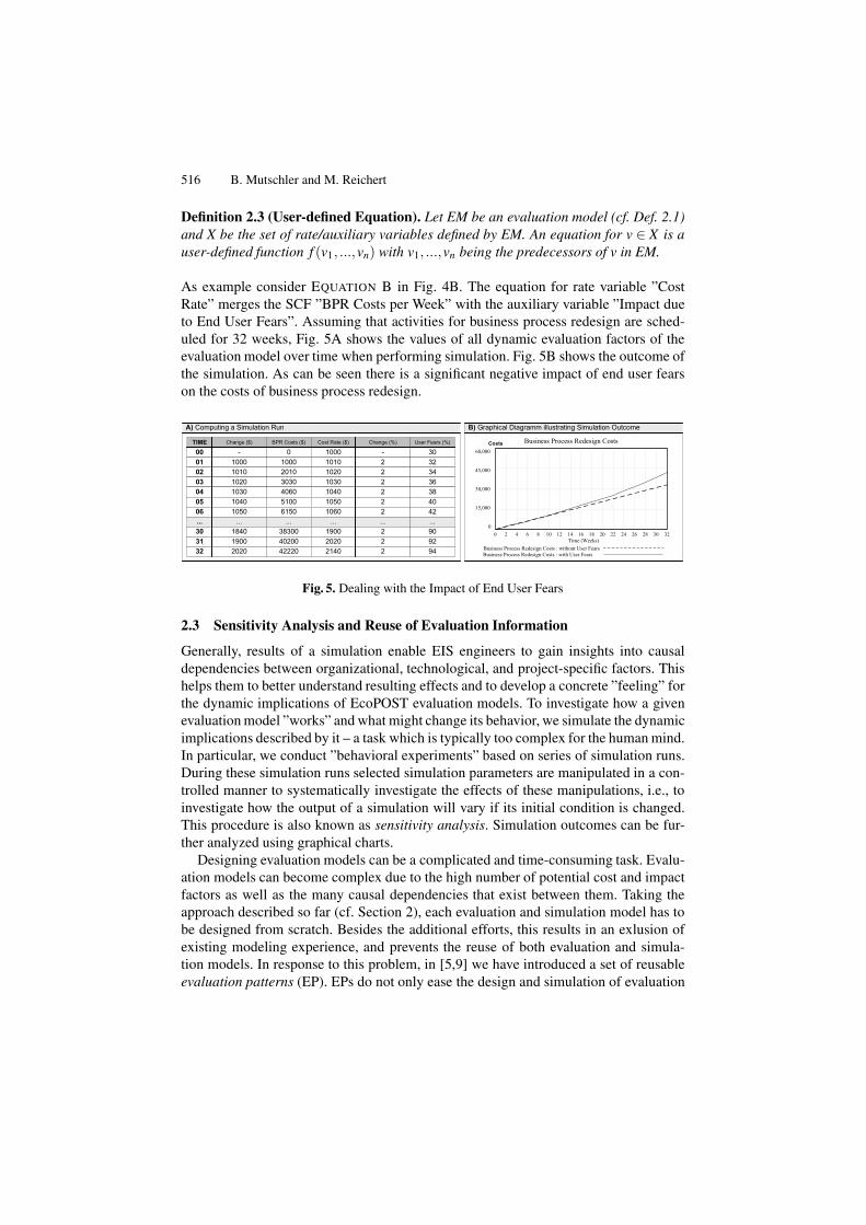
Definition 2.3 (User-defined Equation). Let EM be an evaluation model (cf. Def. 2.1)and X be the set of rate/auxiliary variables defined by EM. An equation for v ∈ X is auser-defined function f (v1, ...,vn) with v1, ...,vn being the predecessors of v in EM.

As example consider EQUATION B in Fig. 4B. The equation for rate variable ”CostRate” merges the SCF ”BPR Costs per Week” with the auxiliary variable ”Impact dueto End User Fears”. Assuming that activities for business process redesign are sched-uled for 32 weeks, Fig. 5A shows the values of all dynamic evaluation factors of theevaluation model over time when performing simulation. Fig. 5B shows the outcome ofthe simulation. As can be seen there is a significant negative impact of end user fearson the costs of business process redesign.

A) Computing a Simulation Run

TIME Change ($) BPR Costs ($)

00 - 001 1000 100002 1010 201003 1020 303004 1030 406005 1040 510006 1050 6150... ... ...30 1840 3830031 1900 4020032 2020 42220

Business Process Redesign Costs

60,000

45,000

30,000

15,000

0

0 2 4 6 8 10 12 14 16 18 20 22 24 26 28 30 32Time (Weeks)

Business Process Redesign Costs : without User Fears

Cost Rate ($)

1000101010201030104010501060

...190020202140

Change (%)

-222222...222

User Fears (%)

30323436384042...909294

B) Graphical Diagramm illustrating Simulation Outcome

Business Process Redesign Costs : with User Fears

Costs

Fig. 5. Dealing with the Impact of End User Fears

2.3 Sensitivity Analysis and Reuse of Evaluation Information

Generally, results of a simulation enable EIS engineers to gain insights into causaldependencies between organizational, technological, and project-specific factors. Thishelps them to better understand resulting effects and to develop a concrete ”feeling” forthe dynamic implications of EcoPOST evaluation models. To investigate how a givenevaluation model ”works” and what might change its behavior, we simulate the dynamicimplications described by it – a task which is typically too complex for the human mind.In particular, we conduct ”behavioral experiments” based on series of simulation runs.During these simulation runs selected simulation parameters are manipulated in a con-trolled manner to systematically investigate the effects of these manipulations, i.e., toinvestigate how the output of a simulation will vary if its initial condition is changed.This procedure is also known as sensitivity analysis. Simulation outcomes can be fur-ther analyzed using graphical charts.

Designing evaluation models can be a complicated and time-consuming task. Evalu-ation models can become complex due to the high number of potential cost and impactfactors as well as the many causal dependencies that exist between them. Taking theapproach described so far (cf. Section 2), each evaluation and simulation model has tobe designed from scratch. Besides the additional efforts, this results in an exlusion ofexisting modeling experience, and prevents the reuse of both evaluation and simula-tion models. In response to this problem, in [5,9] we have introduced a set of reusableevaluation patterns (EP). EPs do not only ease the design and simulation of evaluation


models, but also enable the reuse of evaluation information. This is crucial to foster thepractical applicability of the EcoPOST framework.

3 Model Design Rules

Overall benefit of EcoPOST evaluation models depends on their quality. The latter,in turn, is determined by the syntactical as well as the semantical correctness of theevaluation model. Maintaining correctness of an evaluation model, however, can be adifficult task to accomplish. This section picks up this problem.

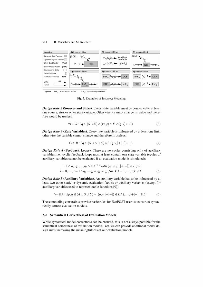
3.1 Modeling Constraints for Evaluation Models

Rules for the correct use of flows and links are shown in Fig. 6A and Fig. 6B. Bycontrast, Fig. 7A – Fig. 7F show examples of incorrect models.

B) Use of Links

SCFDCF

ImFD

ImFS

A

A R

Dependent Variable

SCF DCF ImFD ImFS X

x xxx xx xx xx xxx xx xxx x

xxx x xcorrect link

incorrect link

A) Use of Flows

DCF

ImFD

X

SCF DCF

Inde

pend

ent

Var

iabl

e*

Dependent Variable

ImFD ImFS X

xxx xxxx

x xxx

xcorrect flow incorrect flow

A R

x xx

x

* SCF, ImFS, A and R do not have to be considered here. Flows are only con-nected to dynamic evaluation factors (i.e., DCF and ImFD) and Sources/Sinks.

ImFD = Dynamic ImF ImFS = Static ImF

ImFD = Dynamic ImF

ImFS = Static ImF

*

*

* such links are only allowed if the dependent SCF and ImFS are constants which consistthemselves of subsidiary constants.

Fig. 6. Using Flows and Links in our Evaluation Models

Dynamic evaluation factors, for example, may be only influenced by flows and not bylinks as shown in Fig. 7A. Likewise, flows must be not connected to auxiliary variablesor constants (cf. Fig. 7B). Links pointing from DCFs (or auxiliary variables) to SCFsor static ImFs (cf. Fig. 7C and Fig. 7D) are also not valid as SCFs as well as static ImFshave constant values which cannot be influenced. Finally, flows and links connectingDCFs with dynamic ImFs (and vice versa) are also not considered as correct (cf. Fig.7E and Fig. 7F).

Several other constraints have to be taken into account as well when designing evalu-ation models. In the following let EM = (V, F, L) be an evaluation model (cf. Definition2.1). Then:

Design Rule 1 (Binary Relations). Every model variable must be used in at least onebinary relation. Otherwise, it is not part of the analyzed evaluation context and can beomitted:

∀v ∈ (S ∪ X) : ∃q ∈ (S ∪ X)∧ ((v,q) ∈ F ∨ (v,q) ∈ F) (1)

∀v ∈ (A ∪ C) : ∃q ∈ (A ∪ R)∧∃ (q,v, [+|−]) ∈ L (2)


A) Incorrect LinkNotation

Flows

Auxiliary Variables

Rate Variables

Dynamic Cost Factors

Links

Sources and Sinks


Text

[+|-]


Static Impact Factor (Text)

B) Incorrect Flow C) Incorrect Link

D) Incorrect Flow E) Incorrect Flow F) Incorrect Link

DCF

[SCF]+ Auxiliary

Variable

(ImFS)

ImFD

(ImFS)+ ImFD DCF

ImFDDCF

ImFD DCF

ImFDDCF +

+

DCF

[SCF]+

Caption: ImFS - Static Impact Factor ImFD - Dynamic Impact Factor

Fig. 7. Examples of Incorrect Modeling

Design Rule 2 (Sources and Sinks). Every state variable must be connected to at leastone source, sink or other state variable. Otherwise it cannot change its value and there-fore would be useless:

∀v ∈ S : ∃q ∈ (S ∪ X)∧ ((v,q) ∈ F ∨ (q,v) ∈ F) (3)

Design Rule 3 (Rate Variables). Every rate variable is influenced by at least one link;otherwise the variable cannot change and therefore is useless:

∀v ∈ R : ∃q ∈ (S ∪ A ∪ C)∧∃ (q,v, [+|−]) ∈ L (4)

Design Rule 4 (Feedback Loops). There are no cycles consisting only of auxiliaryvariables, i.e., cyclic feedback loops must at least contain one state variable (cycles ofauxiliary variables cannot be evaluated if an evaluation model is simulated):

¬∃ < q0,q1, ...,qr >∈ Ar+1 with (qi,qi+1, [+|−]) ∈ L f or

i = 0, . . . ,r − 1 ∧q0 = qr ∧ qk = ql f or k, l = 1, . . . ,r;k = l (5)

Design Rule 5 (Auxiliary Variables). An auxiliary variable has to be influenced by atleast two other static or dynamic evaluation factors or auxiliary variables (except forauxiliary variables used to represent table functions [9]):

∀v ∈ A : ∃p,q ∈ (A ∪ S ∪ C)∧ ((q,v, [+|−]) ∈ L∧ (p,v, [+|−]) ∈ L) (6)

These modeling constraints provide basic rules for EcoPOST users to construct syntac-tically correct evaluation models.

3.2 Semantical Correctness of Evaluation Models

While syntactical model correctness can be ensured, this is not always possible for thesemantical correctness of evaluation models. Yet, we can provide additional model de-sign rules increasing the meaningfulness of our evaluation models.


Design Rule 6 (Transitive Dependencies). Transitive link dependencies (i.e., indirecteffects described by chains of links) are restricted. As example consider Fig. 8. Fig.8A reflects the assumption that increasing end user fears result in increasing emotionalresistance. This, in turn, leads to increasing business process costs. Consequently, themodeled transitive dependency between ”End User Fears” and ”Business Process Re-design Costs” is not correct, as increasing end user fears do not result in decreasingbusiness process (re)design costs. The correct transitive dependency is shown in Fig.8B. Fig. 8C illustrates the assumption that increasing process knowledge results in anincreasing ability to (re)design business processes. An increasing ability to (re)designbusiness processes, in turn, leads to decreasing process definition costs. The modeledtransitive dependency between ”Process Knowledge” and ”Process Definition Costs”,however, is not correct, as increasing process knowledge does not result in increasingprocess definition costs (assuming that the first 2 links are correct). The correct transi-tive dependency is shown in Fig. 8D.

A) Incorrect Transitive Dependency

C) Incorrect Transitive Dependency

B) Correct Transitive Dependency

(ProcessKnowledge)

(Ability to redesignBusiness Processes)

+[Process

Definition Costs]

-

+

D) Correct Transitive Dependency

(ProcessKnowledge)

(Ability to redesignBusiness Processes)

+[Process

Definition Costs]

-

-

(End UserFears)

(EmotionalResistance)

+[Business ProcessRedesign Costs]

+

-

(End UserFears)

(EmotionalResistance)

+(Management

Pressure)

+

+

E) Incorrect Transitive Dependency F) Correct Transitive Dependency

(Communication) (End UserFears)

-(Ability to redesign

Business Processes)

-

+(Communication) (End User

Fears)

-(Ability to redesign

Business Processes)

-

-

Fig. 8. Transitive Dependencies (Simplified Evaluation Models)

Finally, Fig. 8E deals with the impact of communication (e.g., the goals of an EISproject) on the ability to redesign business processes. Yet, the transitive dependencyshown in Fig. 8E is not correct. The correct one is shown in Fig. 8F.

Altogether, two causal relations (”+” and ”-”) are used in the context of our evalua-tion models. Correct transitive dependencies can be described based on a multiplicationoperator. More precisely, transitive dependencies have to comply with the followingthree multiplication laws for transitive dependencies (for any x,y ∈ {+,−}):

+∗y = y (7)

−∗− = + (8)

x ∗ y = y ∗ x (9)

The evaluation models shown in Fig. 8A and Fig. 8C violate Law 1, whereas the modelshown in Fig. 8E violates the second one. Law 3 states that the ”*” is commutative.

Design Rule 7 (Dual Links I). A constant cannot be connected to the same auxiliaryvariable with both a positive and negative link:


∀v ∈ C,∀q ∈ A : ¬∃ l1, l2 ∈ L withl1 = (v,q,−)∧ l2 = (v,q,+) (10)

Design Rule 8 (Dual Links II). A state variable cannot be connected to the same aux-iliary variable with both a positive and negative link:

∀v ∈ S,∀q ∈ A : ¬∃ l1, l2 ∈ L withl1 = (v,q,−)∧ l2 = (v,q,+) (11)

Design Rule 9 (Dual Links III). An auxiliary variable cannot be connected to anotherauxiliary variable with both a positive and negative link:

∀v ∈ A,∀q ∈ A : ¬∃ l1, l2 ∈ L withl1 = (v,q,−)∧ l2 = (v,q,+) (12)

Finally, there exist two additional simple constraints:

Design Rule 10 (Representing Cost Factors). A cost factor cannot be represented bothas SCF and DCF in one evaluation model.

Design Rule 11 (Representing Impact Factors). An impact factor cannot be repre-sented both as static and dynamic ImF in one evaluation model.

Without providing model design rules, incorrect evaluation models can be quickly mod-eled. This, in turn, does not only aggravate the derivation of plausible evaluations, butalso hampers the use of the modeling and simulation tools [5] which have been devel-oped as part of the EcoPOST framework.

4 Modeling Guidelines

To further facilitate the use of our methodology, governing guidelines and best practicesare provided. This section summarizes two categories of EcoPOST governing guide-lines: (1) guidelines for evaluation models and (2) guidelines for simulation models.

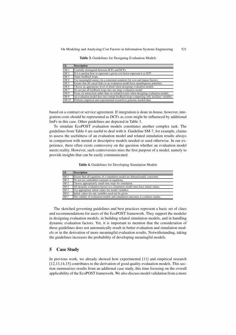
In general, EcoPOST evaluation models can become large, e.g., due to a potentiallyhigh number of evaluation factors to be considered or due to the large number of causaldependencies existing between them. To cope with this complexity, we introduce guide-lines for designing evaluation models (cf. Table 3). Their derivation is based on expe-riences we gathered during the development of our approach, its initial use in practice,and our study of general System Dynamics (SD) guidelines [10]. As example considerguideline EM-1 from Table 3. The distinction between SCFs and DCFs is a fundamen-tal principle in the EcoPOST framework. Yet, it can be difficult for the user to decidewhether a cost factor shall be considered as static or dynamic. As example take an evalu-ation scenario which deals with the introduction of a new EIS ”CreditLoan” to supportthe granting of loans at a bank. Based on the new EIS, the entire loan offer processshall be supported. For this purpose, the EIS has to leverage internal (i.e., within thebank) and external (e.g., a dealer) trading partners as well as other legacy applicationsfor customer information and credit ratings. Among other things, this necessitates theintegration of existing legacy applications. In case this integration is done by externalsuppliers, resulting costs can be represented as SCFs as they can be clearly quantified


Table 3. Guidelines for Designing Evaluation Models

GL Description

EM-1 Carefully distinguish between SCFs and DCFs.EM-2 If it is unclear how to represent a given cost factor represent it as SCF.EM-3 Name feedback loops.EM-4 Use meaningful names (in a consistent notation) for cost and impact factors.EM-5 Ensure that all causal links in an evaluation model have unambiguous polarities.EM-6 Choose an appropriate level of detail when designing evaluation models.EM-7 Do not put all feedback loops into one large evaluation model.EM-8 Focus on interaction rather than on isolated events when designing evaluation models.EM-9 An evaluation model does not contain feedback loops comprising only auxiliary variables.EM-10 Perform empirical and experimental research to generate needed data.

based on a contract or service agreement. If integration is done in-house, however, inte-gration costs should be represented as DCFs as costs might be influenced by additionalImFs in this case. Other guidelines are depicted in Table 3.

To simulate EcoPOST evaluation models constitutes another complex task. Theguidelines from Table 4 are useful to deal with it. Guideline SM-7, for example, claimsto assess the usefulness of an evaluation model and related simulation results alwaysin comparison with mental or descriptive models needed or used otherwise. In our ex-perience, there often exists controversy on the question whether an evaluation modelmeets reality. However, such controversies miss the first purpose of a model, namely toprovide insights that can be easily communicated.

Table 4. Guidelines for Developing Simulation Models

GL Description

SM-1 Ensure that all equations of a simulation model are dimensionally consistent.SM-2 Do not use embedded constants in equations.SM-3 Choose appropriately small time steps for simulation.SM-4 All dynamic evaluation factors in a simulation model must have initial values.SM-5 Use appropriate initial values for model variables.SM-6 Initial values for rate variables need not be given.SM-7 The validity of evaluation models and simulation outcomes is a relative matter.

The sketched governing guidelines and best practices represent a basic set of cluesand recommendations for users of the EcoPOST framework. They support the modelerin designing evaluation models, in building related simulation models, and in handlingdynamic evaluation factors. Yet, it is important to mention that the consideration ofthese guidelines does not automatically result in better evaluation and simulation mod-els or in the derivation of more meaningful evaluation results. Notwithstanding, takingthe guidelines increases the probability of developing meaningful models.

5 Case Study

In previous work, we already showed how experimental [11] and empirical research[12,13,14,15] contributes to the derivation of good quality evaluation models. This sec-tion summarizes results from an additonal case study, this time focusing on the overallapplicability of the EcoPOST framework. We also discuss model validation from a more


general viewpoint. Due to space limitations we cannot decsribe the complete case studyin detail (for details see [9]).

5.1 Research Design

We apply the EcoPOST framework to a complex EIS engineering project from theautomotive domain in which we participated. We investigate cost overruns observedduring the introduction of a large information system for supporting the developmentof electrical and electronic (E/E) systems (e.g., a multimedia unit in the car). Basedon real project data, interviews with project members (e.g., requirements engineers,software architects, software developers), online surveys among end users, and practicalexperiences gathered in the respective EIS engineering project, we develop a set ofEcoPOST evaluation models and analyze these models using simulation.

An initial business case for the considered EIS engineering project is developed priorto project start in order to convince senior management to fund the project. This busi-ness case is based on data about similar projects provided by competitors (evaluationby analogy) as well as on rough estimates on planned costs and assumed benefits ofthe project. The business case comprises six main cost categories: (1) project manage-ment, (2) process management, (3) IT system realization, (4) specification and test, (5)roll-out and migration, and (6) implementation of interfaces.

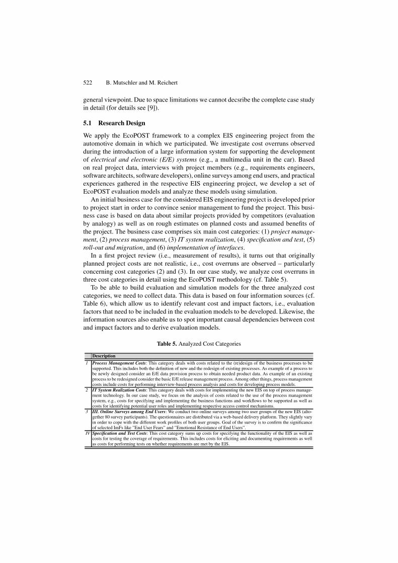
In a first project review (i.e., measurement of results), it turns out that originallyplanned project costs are not realistic, i.e., cost overruns are observed – particularlyconcerning cost categories (2) and (3). In our case study, we analyze cost overruns inthree cost categories in detail using the EcoPOST methodology (cf. Table 5).

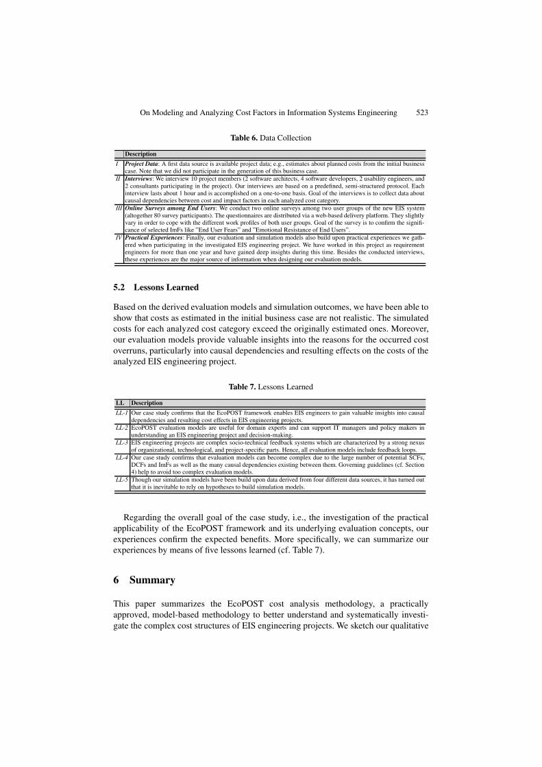
To be able to build evaluation and simulation models for the three analyzed costcategories, we need to collect data. This data is based on four information sources (cf.Table 6), which allow us to identify relevant cost and impact factors, i.e., evaluationfactors that need to be included in the evaluation models to be developed. Likewise, theinformation sources also enable us to spot important causal dependencies between costand impact factors and to derive evaluation models.

Table 5. Analyzed Cost Categories

Description

1 Process Management Costs: This category deals with costs related to the (re)design of the business processes to besupported. This includes both the definition of new and the redesign of existing processes. As example of a process tobe newly designed consider an E/E data provision process to obtain needed product data. As example of an existingprocess to be redesigned consider the basic E/E release management process. Among other things, process managementcosts include costs for performing interview-based process analysis and costs for developing process models.

2 IT System Realization Costs: This category deals with costs for implementing the new EIS on top of process manage-ment technology. In our case study, we focus on the analysis of costs related to the use of the process managementsystem, e.g., costs for specifying and implementing the business functions and workflows to be supported as well ascosts for identifying potential user roles and implementing respective access control mechanisms.

3 III. Online Surveys among End Users: We conduct two online surveys among two user groups of the new EIS (alto-gether 80 survey participants). The questionnaires are distributed via a web-based delivery platform. They slightly varyin order to cope with the different work profiles of both user groups. Goal of the survey is to confirm the significanceof selected ImFs like ”End User Fears” and ”Emotional Resistance of End Users”.

IV Specification and Test Costs: This cost category sums up costs for specifying the functionality of the EIS as well ascosts for testing the coverage of requirements. This includes costs for eliciting and documenting requirements as wellas costs for performing tests on whether requirements are met by the EIS.


Table 6. Data Collection

Description

I Project Data: A first data source is available project data; e.g., estimates about planned costs from the initial businesscase. Note that we did not participate in the generation of this business case.

II Interviews: We interview 10 project members (2 software architects, 4 software developers, 2 usability engineers, and2 consultants participating in the project). Our interviews are based on a predefined, semi-structured protocol. Eachinterview lasts about 1 hour and is accomplished on a one-to-one basis. Goal of the interviews is to collect data aboutcausal dependencies between cost and impact factors in each analyzed cost category.

III Online Surveys among End Users: We conduct two online surveys among two user groups of the new EIS system(altogether 80 survey participants). The questionnaires are distributed via a web-based delivery platform. They slightlyvary in order to cope with the different work profiles of both user groups. Goal of the survey is to confirm the signifi-cance of selected ImFs like ”End User Fears” and ”Emotional Resistance of End Users”.

IV Practical Experiences: Finally, our evaluation and simulation models also build upon practical experiences we gath-ered when participating in the investigated EIS engineering project. We have worked in this project as requirementengineers for more than one year and have gained deep insights during this time. Besides the conducted interviews,these experiences are the major source of information when designing our evaluation models.

5.2 Lessons Learned

Based on the derived evaluation models and simulation outcomes, we have been able toshow that costs as estimated in the initial business case are not realistic. The simulatedcosts for each analyzed cost category exceed the originally estimated ones. Moreover,our evaluation models provide valuable insights into the reasons for the occurred costoverruns, particularly into causal dependencies and resulting effects on the costs of theanalyzed EIS engineering project.

Table 7. Lessons Learned

LL Description

LL-1 Our case study confirms that the EcoPOST framework enables EIS engineers to gain valuable insights into causaldependencies and resulting cost effects in EIS engineering projects.

LL-2 EcoPOST evaluation models are useful for domain experts and can support IT managers and policy makers inunderstanding an EIS engineering project and decision-making.

LL-3 EIS engineering projects are complex socio-technical feedback systems which are characterized by a strong nexusof organizational, technological, and project-specific parts. Hence, all evaluation models include feedback loops.

LL-4 Our case study confirms that evaluation models can become complex due to the large number of potential SCFs,DCFs and ImFs as well as the many causal dependencies existing between them. Governing guidelines (cf. Section4) help to avoid too complex evaluation models.

LL-5 Though our simulation models have been build upon data derived from four different data sources, it has turned outthat it is inevitable to rely on hypotheses to build simulation models.

Regarding the overall goal of the case study, i.e., the investigation of the practicalapplicability of the EcoPOST framework and its underlying evaluation concepts, ourexperiences confirm the expected benefits. More specifically, we can summarize ourexperiences by means of five lessons learned (cf. Table 7).

6 Summary

This paper summarizes the EcoPOST cost analysis methodology, a practicallyapproved, model-based methodology to better understand and systematically investi-gate the complex cost structures of EIS engineering projects. We sketch our qualitative


EcoPOST methodology, introduce model design rules and describes modeling guide-lines. We also summarize a case study illustrating the benefits of our approach.

Currently, our methodology is used in various information system engineering pro-jects, mainly in the automotive domain. In future, we want to further validate our ap-proach and aim at increasing the number of EcoPOST evaluation patterns [9].

References

1. Reijers, H.A., van der Aalst, W.M.P.: The Effectiveness of Workflow Management Systems- Predictions and Lessons Learned. Int’l. J. of Inf. Mgmt. 25(5), 457–471 (2005)

2. Boehm, B., Abts, C., Brown, A.W., Chulani, S., Clark, B.K., Horowitz, E., Madachy, R.,Reifer, D., Steece, B.: Software Cost Estimation with Cocomo 2. Prentice-Hall, EnglewoodCliffs (2000)

3. Mutschler, B., Reichert, M., Bumiller, J.: Designing an Economic-driven Evaluation Frame-work for Process-oriented Software Technologies. In: Proc. 28th ICSE, pp. 885–888 (2006)

4. Mutschler, B., Zarvic, N., Reichert, M.: A Survey on Economic-driven Evaluations of Infor-mation Technology. Technical Report, TR-CTIT-07, University of Twente (2007)

5. Mutschler, B., Reichert, M., Rinderle, S.: Analyzing the Dynamic Cost Factors of Process-aware Information Systems: A Model-based Approach. In: 19th CAiSE, pp. 589–603 (2007)

6. Richardson, G.P., Pugh, A.L.: System Dynamics - Modeling with DYNAMO (1981)7. Forrester, J.W.: Industrial Dynamics, Industrial Dynamics. Productivity Press (1961)8. Systems, V.: Vensim (2006), http://www.vensim.com/9. Mutschler, B.: Analyzing Causal Dependencies on Process-aware Information Systems from

a Cost Perspective. PhD Thesis, University of Twente (2008)10. Sterman, J.D.: Business Dynamics. McGraw-Hill, New York (2000)11. Mutschler, B., Weber, B., Reichert, M.: Workflow Management versus Case Handling: Re-

sults from a Controlled Software Experiment. In: Proc. ACM SAC 2008 (2008)12. Mutschler, B., Reichert, M., Bumiller, J.: Unleashing the Effectiveness of Process-oriented

Infomation Systems: Problem Analysis, Critical Success Factors and Implications. IEEETransactions on Systems, Man, and Cybernetics (2008)

13. Mutschler, B., Rijkpema, M., Reichert, M.: Investigating Implemented Process Design: ACase Study on the Impact of Process-aware Information Systems on Core Job Dimensions.In: Proc. 8th Int’l. BPMDS Workshop, pp. 379–384 (2007)

14. Mutschler, B., Reichert, M.: A Survey on Evaluation Factors for Business Process Manage-ment Technology. Technical Report, TR-CTIT-06-63, University of Twente (2006)

15. Mutschler, B., Reichert, M., Bumiller, J.: Why Process-Orientation is Scarce: An EmpiricalStudy of Process-oriented Information Systems in the Automotive Industry. In: Proc. 10thIEEE EDOC, pp. 433–438 (2006)

http://www.vensim.com/

on modeling and analyzing cost factors in information...

Documents