on multidisciplinary panel data research 2
TRANSCRIPT

Deutsches Institut für Wirtschaftsforschung
www.diw.de
Frank M. Fossen • Davud Rostam-Afschar
EPrecautionary and Entrepreneurial Saving –New Evidence from German Households Ts
240
SOEPpaperson Multidisciplinary Panel Data Research
Berlin, November 2009
SOEPpapers on Multidisciplinary Panel Data Research at DIW Berlin This series presents research findings based either directly on data from the German Socio-Economic Panel Study (SOEP) or using SOEP data as part of an internationally comparable data set (e.g. CNEF, ECHP, LIS, LWS, CHER/PACO). SOEP is a truly multidisciplinary household panel study covering a wide range of social and behavioral sciences: economics, sociology, psychology, survey methodology, econometrics and applied statistics, educational science, political science, public health, behavioral genetics, demography, geography, and sport science. The decision to publish a submission in SOEPpapers is made by a board of editors chosen by the DIW Berlin to represent the wide range of disciplines covered by SOEP. There is no external referee process and papers are either accepted or rejected without revision. Papers appear in this series as works in progress and may also appear elsewhere. They often represent preliminary studies and are circulated to encourage discussion. Citation of such a paper should account for its provisional character. A revised version may be requested from the author directly. Any opinions expressed in this series are those of the author(s) and not those of DIW Berlin. Research disseminated by DIW Berlin may include views on public policy issues, but the institute itself takes no institutional policy positions. The SOEPpapers are available at http://www.diw.de/soeppapers Editors: Georg Meran (Dean DIW Graduate Center) Gert G. Wagner (Social Sciences) Joachim R. Frick (Empirical Economics) Jürgen Schupp (Sociology)
Conchita D’Ambrosio (Public Economics) Christoph Breuer (Sport Science, DIW Research Professor) Anita I. Drever (Geography) Elke Holst (Gender Studies) Martin Kroh (Political Science and Survey Methodology) Frieder R. Lang (Psychology, DIW Research Professor) Jörg-Peter Schräpler (Survey Methodology) C. Katharina Spieß (Educational Science) Martin Spieß (Survey Methodology, DIW Research Professor) ISSN: 1864-6689 (online) German Socio-Economic Panel Study (SOEP) DIW Berlin Mohrenstrasse 58 10117 Berlin, Germany Contact: Uta Rahmann | [email protected]
Precautionary and EntrepreneurialSavinga
–New Evidence from German Households
Frank M. Fossenb Davud Rostam-Afscharc
September 2, 2009
Abstract
The well-documented positive correlation between income risk and wealth was interpreted as
evidence for high amounts of precautionary wealth in various studies. However, the large
estimates emerged from pooling non-entrepreneurs and entrepreneurs without controlling for
heterogeneity. This paper provides evidence for Germany based on representative panel data
including private wealth balance sheets. Entrepreneurs, who face high income risk, hold
more wealth than employees, but it is shown that this is not due to precautionary motives.
Entrepreneurs may rather save for old age, as they are usually not covered by statutory
pension insurance. The analysis accounts for endogeneity of entrepreneurial choice.
Keywords: precautionary saving, precautionary wealth, entrepreneurshipJEL: D91, D12, E21
a The authors would like to thank Viktor Steiner and participants in a joint seminar of DIW Berlin and theFree University of Berlin for valuable comments and suggestions. Financial support from the GermanResearch Foundation (DFG) for the project "Tax Policy and Entrepreneurial Choice" (STE 681/7-1) isgratefully acknowledged. The usual disclaimer applies.
b DIW Berlin, e-mail: [email protected] DIW Berlin and Free University of Berlin, e-mail: [email protected]

Precautionary and Entrepreneurial Saving 1
1. Introduction
Various studies have suggested that a large share of the wealth of households can be explained
by a precautionary saving motive. Quantity estimates of precautionary savings are important
because of their implications for policies that affect income risk, particularly labor market,
social security and taxation policy. If the precautionary saving motive is strong, policies that
increase income risk will raise savings, which in turn is likely to influence the growth rate of
an economy (e.g. Femminis, 2001).
A widely applied estimation approach is to use the relationship between the income risk
of households and their wealth holdings to quantify the fraction of wealth which is held as
precaution against systematic uncertainty. If the stock of wealth is positively related to income
variations, this is interpreted as evidence for the existence of precautionary saving. Applying
this method to panel data from the USA, Kazarosian (1997) found a strong precautionary
saving motive, and Carroll and Samwick (1997, 1998) reported that precautionary savings
even amount to almost half of American households’ wealth. By analyzing data on the
subjective assessment of risks, Lusardi (1997, 1998) cast doubt on these high estimates.
Hurst et al. (forthcoming) showed that the precautionary saving motive was overestimated
in previous literature that did not properly account for heterogeneity between entrepreneurial
and non-entrepreneurial households. Entrepreneurs hold more wealth, face higher income
risk and differ in their saving motives from other households. Explicitly taking account of the
special role of entrepreneurial households, Hurst et al. (forthcoming) estimated precautionary
wealth to represent less than ten percent of overall wealth in the USA. They were also able
to show that large estimates of precautionary savings reported by prior studies resulted from
pooling together entrepreneurial and non-entrepreneurial households and vanish if the sample
is split, or controls for entrepreneurial households are introduced.
This paper adds to this evolving literature by providing the first analysis of the existence
and quantity of precautionary savings explicitly accounting for entrepreneurship in Germany.
The findings reported by Hurst et al. (forthcoming) for the USA turn out to be even more
2 Precautionary and Entrepreneurial Saving
important in Germany: Using our preferred specifications, no statistically significant evidence
of precautionary saving remains once entrepreneurship is accounted for, and when the
dependent variable is total net worth (with or without business wealth), rather than just
financial wealth. The analysis is based on the Socio-Economic Panel (SOEP), which has the
crucial advantages of providing information on private wealth balance sheets and individual
measures of risk aversion.
By focusing on Germany, this study examines the importance of accounting for entrepreneur-
ship when estimating precautionary savings in a country where employees, as opposed to
entrepreneurs, are covered by an extensive social security system. In particular, saving
behavior may differ between entrepreneurs and non-entrepreneurs even more than in the
USA because employees are covered by statutory pension insurance, whereas entrepreneurs
have to save for their old age consumption.
Fuchs-Schündeln and Schündeln (2005) and Bartzsch (2008) identified about one fifth
of household wealth in Germany as precautionary, using different strategies to control for
risk aversion. They employed the same data as in this analysis, the German SOEP. Upon
re-examination, their results could represent portfolio decisions in favor of liquid assets
rather than precautionary saving, because they find an influence of uncertainty on financial
assets only, which represent the most liquid component of a household’s wealth portfolio.
Essig (2005) and Schunk (2007) used the German SAVE dataset of the Mannheim Research
Institute for the Economics of Aging (MEA) to relate saving behavior to motives which are
elicited based on subjective importance measures. One of Essig’s (2005) findings is a higher
savings rate of the self-employed. In line with our reasoning, he doubts this can be attributed
to uncertainty.
The main methodological contribution of this paper beyond Hurst et al. (forthcoming) is
that entrepreneurial status is recognized and treated as being endogenous with respect to
wealth. Endogeneity may arise from credit constraints faced by nascent entrepreneurs, for
example, as more wealthy people are more likely to be able to enter entrepreneurship. To
deal with this, the wealth equations of entrepreneurs and non-entrepreneurs are modeled as
Precautionary and Entrepreneurial Saving 3
an endogenous switching regression, among other specifications.
The following section presents the empirical methodology employed to test the hypothesis
of precautionary saving. In Section 3, different strategies are suggested how entrepreneurship
can be accounted for appropriately. A description of the data follows in Section 4. The
main analysis is conducted in two stages. First, we construct measures of permanent income
and of income uncertainty, as described in Section 5. Second, we estimate wealth equations.
Section 6 presents the results, which are discussed in Section 7, and Section 8 concludes.
2. Empirical Specification
The estimation equation is motivated by the buffer-stock model developed by Deaton (1991)
and Carroll (1992, 1997, 2004). The model’s main feature is a target wealth-to-income
ratio, which describes a positive relation between wealth W and permanent income P that
consumers want to maintain. If wealth is above the target, consumption will exceed income
and wealth will fall. If wealth is below the target, income will exceed consumption and wealth
will rise.1 According to the model, the size of the wealth target depends on the degree of
uncertainty ω a consumer faces.2 Additionally, target wealth may be shifted by a vector of
observed characteristics x and an unobserved error term u:
W
P= f(ω,x,u). (1)
As wealth and income are highly unequally distributed, natural logarithms are chosen for the
empirical specification:
ln(Wit) = α0 + γ′ωit + α1ln(Pit) + β′xit + uit (2)
1 This would explain why the saving rate increased in the USA, after wealth balances shrunk during therecent financial turmoil. Since the beginning of 2005 to April 2008 the seasonally adjusted annual personalsaving rate as provided by the Bureau of Economic Analysis of the U.S. Department of Commerceremained quite stable at an average of 1.8%. From May 2008 on, when the financial crisis had hit theeconomy, savers reacted by accumulating 3.9% on average till June 2009, the end of the reporting period.
2 In this general notation ω is written as a vector, because in one specification we decompose income riskinto permanent and transitory components (see Section 4).
4 Precautionary and Entrepreneurial Saving
The equation is estimated at the household level, because household members are likely to
take saving decisions jointly based on pooled income. Thus, P denotes permanent household
income.3 We measureW as total net worth, i.e. total assets of the household minus total debt.
In contrast to analyzing wealth components, e.g. financial assets, this avoids mixing saving
with portfolio decisions. Wealth components will be examined additionally for comparison
with the literature. The vector x contains characteristics of the household or household head
as control variables. It includes age, age squared, years in unemployment and its square,
work experience and its square, and dummy variables indicating gender, marital status,
the number of children under 17 in the household, nationality, region, disability, and the
year of observation. Additionally, 10 dummy variables representing the self-reported risk
attitude on a scale from 0 to 10 are included, similarly to Bartzsch (2008). This controls for
self-selection of more risk tolerant people into occupations with higher income risk, which
might otherwise lead to a downward selection bias in the coefficient of the income variance.
In a field experiment with real money at stake, based on a representative sample of 450
subjects, Dohmen et al. (2005) found that these survey measures of the willingness to take
risks are good predictors of actual risk-taking behavior.4
The buffer-stock model predicts α1 > 0. With respect to γ, the theoretical proposition
is a positive value,5 as the optimal reaction to greater uncertainty is to hold more wealth.
This corresponds to the existence of a precautionary saving motive. The different uncertainty
measures used will be described in Section 4. In the following section, the specification is
further elaborated on to account for the specific role of entrepreneurship.
3 We assume that households regard uncertainty in terms of variation in net rather than gross income. Thisis an important distinction, because gross income’s variation is reduced by progressive taxation.
4 Since information on risk attitudes are only available in the SOEP waves 2004 and 2006, while the mainanalysis is based on the years 2002 and 2007 (see Section 4), the attitudes in 2002 are approximated bythe observations in 2004 and in 2007 by the observations in 2006.
5 Respectively, positive components of γ, if the decomposed measure of uncertainty is used.
Precautionary and Entrepreneurial Saving 5
3. Dealing with Entrepreneurs
As mentioned in the introduction, Carroll and Samwick (1997, 1998) presented estimation
results for the USA which indicated that almost 50% of total net worth is due to the
precautionary motive. They used occupational categories, which included self-employed
managers, as instruments for their measures of earnings risk and permanent income. The
approach requires the strong assumption that entrepreneurship has no direct influence
on wealth. The authors identified the self-employed as crucial for their high estimate of
precautionary savings: When they excluded farmers and the self-employed from the sample,
their estimations showed almost no support for the existence of precautionary saving. They
argued that these two groups provided variation in income and hence these groups should
remain in the sample (Carroll and Samwick, 1998, p. 415).
The main critique of this interpretation by Hurst et al. (forthcoming) was that the
correlation between wealth and income uncertainty in the pooled sample is not due to a
precautionary motive rather than to differences between entrepreneurs and non-entrepreneurs,
as entrepreneurs have both higher income variance and more wealth for reasons unrelated to
precautionary savings. They argued that other incentives to save for entrepreneurs could
explain the higher amounts of wealth, such as saving for old-age provision, as the propensity
to have a pension is higher for non-entrepreneurs than for entrepreneurs. Entrepreneurial and
non-entrepreneurial households may also differ in preferences. An entrepreneurial household
could have a different bequest or housing motive or discount factor.
This leads to heterogeneity between entrepreneurs and non-entrepreneurs that has to be
accounted for. There are three potential strategies how to do this:
1. By employing a dummy variable for entrepreneurial households in x.
2. By excluding entrepreneurial households from the sample.
3. By using a measure of wealth W that does not include business equity.
The effect of accounting for entrepreneurship was shown using PSID data for the USA by
Hurst et al. (forthcoming). They demonstrated that the estimated amount of precautionary
6 Precautionary and Entrepreneurial Saving
saving decreases from 50% without accounting for entrepreneurs to less than 10%.
The differences in the savings behavior between entrepreneurs and non-entrepreneurs may
be even larger in Germany because of the more important role of the social security system.
Employees are covered by statutory pension insurance, whereas entrepreneurs usually are not.
Entrepreneurs have to save for their old age consumption, for example by paying into life or
private pension insurance, investing in property, or reinvesting in their own business, all of
which is part of total net worth, the dependent variable. The coefficient of an entrepreneurship
dummy variable captures the additional saving of entrepreneurs that are due to their status
and not to their higher income variance. As entrepreneurship is strongly correlated with a
higher variance of income, omitting the entrepreneurship dummy in the pooled sample leads
to an upward bias of the estimated coefficient of income risk. This leads to an overestimation
of precautionary saving in the whole population.
While solving the omitted variable problem, including an entrepreneurship dummy in x may
introduce another endogeneity problem. If credit constraints exist for nascent entrepreneurs,
wealthier households may be more likely to enter entrepreneurship (e.g. Nykvist, 2008; Hurst
and Lusardi, 2004; Johansson, 2000; Blanchflower and Oswald, 1998). Endogeneity potentially
biases all estimated coefficients, including the coefficient of income risk and thus the estimated
degree of precautionary saving.
We employ the instrumental variables (IV) technique to deal with the endogeneity of the
entrepreneurship dummy in the pooled regression. As instruments, dummy variables are used,
which indicate a self-employed father6 of the household head, whether the household head’s
father and mother had high school diplomas that qualify for university entrance (Abitur),
and the highest educational attainment of the household head.7 Having a self-employed
father is well-known to strongly increase the probability of being an entrepreneur (Dunn and
Holtz-Eakin, 2000).
6 In Germany, self-employed mothers were rare in the generation of most respondents’ parents, and theinformation are often missing, so only self-employed fathers are used.
7 Four levels are distinguished: apprenticeship, technical school degree or Abitur, higher technical collegedegree or similar, and university degree.
Precautionary and Entrepreneurial Saving 7
The GMM IV-estimation based on the pooled sample assumes that the coefficients are the
same for entrepreneurs and non-entrepreneurs. Splitting the sample between entrepreneurs
and non-entrepreneurs is less restrictive as the coefficients are allowed to differ. Estimation
on the sub-sample of non-entrepreneurs then corresponds to the second approach mentioned
above, i.e. excluding entrepreneurs from the sample. For the same reasons that cause the
endogeneity of the entrepreneurship dummy in the pooled regression, splitting the sample
between entrepreneurs and non-entrepreneurs may introduce selectivity bias, as selection into
entrepreneurship is non-random.
Instead of simply splitting the sample we thus employ an endogenous switching regression
model, where entrepreneurs (I = 1) face a different regime than non-entrepreneurs (cf.
Maddala, 1983; Lokshin and Sajaia, 2004):
Iit = 1 if δzit + vit > 0
Iit = 0 if δzit + vit ≤ 0
Regime 1: ln(Wit) = α0,1 + γ′1ωit + α1,1ln(Pit) + β′1xit + u1,it if Iit = 1 (3)
Regime 2: ln(Wit) = α0,2 + γ′2ωit + α1,2ln(Pit) + β′2xit + u2,it if Iit = 0 (4)
The explanatory variables z in the criterion function, which determines selection into
entrepreneurship, include the variables in x and additionally the dummy variables used as IVs
mentioned above. These additional variables thus serve as exclusion restriction here. Under
the assumption that the error terms v, u1 and u2 follow the trivariate normal distribution,
the model is estimated using the maximum likelihood method. We will use a restricted
version of the model, where the coefficients do not differ between the two regimes, to test
for the significance of the difference between the regimes. The restricted model corresponds
to a treatment effects model (Heckman, 1978), where entrepreneurship is understood as the
treatment. Furthermore, as part of the robustness analysis, we will check how excluding
business equity from the wealth measure influences the estimate of precautionary savings
(strategy 3).
8 Precautionary and Entrepreneurial Saving
4. Dataset and Sub-Samples
This analysis is based on data from the Socio-Economic Panel (SOEP), a representative
annual household panel survey in Germany started in 1984. Wagner et al. (2007) provide a
detailed description of the data. We use all waves available (1984-2007) to estimate permanent
income and income uncertainty measures. The waves of 2002 and 2007 included a special
module collecting information about private wealth. Thus, the main analysis refers to these
two periods. The interviewers asked for the market value of personally owned real estate
(owner-occupied housing, other property, mortgage debt), financial assets, tangible assets,
private life and pension insurance, consumer credits, and private business equity (net market
value; own share in case of a business partnership). The wealth balance sheets were elicited at
the personal level. In case of jointly owned assets, the personally owned shares were explicitly
asked for. For the purpose of this analysis, we aggregate wealth and income data to the
household level for the reasons mentioned in Section 2.8
Fuchs-Schündeln and Schündeln (2005) also used the SOEP, but only until the wave of
2000, so direct wealth information was not available. Instead, they relied on the flows of
received amounts of interest and dividend payments to estimate financial wealth using the
yearly average interest and dividend yields in Germany. Apart from the low precision in the
amount of financial wealth estimated this way, another disadvantage of this approach was
that no wealth components other than financial assets could be considered (the implications
will be discussed in Section 7).
An entrepreneurial household is defined as a household owning a private business with
a positive value, as in Hurst et al. (forthcoming). We exclude households whose heads are
younger than 18 or older than 55 from the sample, because youth or older consumers in the
years immediately preceding retirement are not expected to engage in buffer-stock saving (cf.
Carroll, 1997). For the same reason pensioners, individuals in education or vocational training,
8 Apart from that, the personal characteristics of the household’s head are associated with the household.As head of household the earner is determined who has the highest gross monthly income. In case bothearners have exactly the same gross monthly income, the SOEP’s definition of household head is used.
Precautionary and Entrepreneurial Saving 9
interns, those serving in the military or community service, the unemployed, and those not
participating in the labor market are excluded.9 In the sample of 2002 and 2007, 6,303
observations of households-years remain, 474 of which refer to entrepreneurial households.
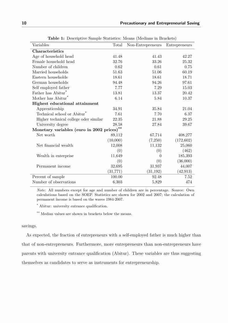
Table 1 provides the means of the variables in this sample and the sub-samples of en-
trepreneurial and non-entrepreneurial households. At the bottom of the table, the means of
total net worth,10 net financial wealth (financial assets minus debt from consumer credits)
and wealth held in private businesses are shown. The latter is zero for non-entrepreneurial
households by definition. All monetary variables are deflated using the consumer price index
provided by the Federal Statistical Office.
It is obvious that entrepreneurial households differ from other households. Their total net
worth is on average more than six times larger than that of non-entrepreneurial households.
This comparison of assets exaggerates the wealth difference between entrepreneurs and the
remaining population, however, as it does not consider the statutory pension insurance
entitlements of the dependently employed in Germany. Assuming an average monthly
pension of 1000 euro and a remaining life expectancy at the age of 65 (retirement age in
Germany) of 18.5 years (Deutsche Rentenversicherung, 2007), average public pension wealth
amounts to 222,000 euro. Thus, on average employees have a lower total net worth than
entrepreneurs even after consideration of public pension wealth, but the gap becomes much
smaller. Entrepreneurs also enjoy a higher level of permanent net income, in part because
usually they do not pay social security contributions (the construction of permanent net
income will be described in the next section).
Another interesting observation is the large share of private business equity in total net
worth of entrepreneurial households (see also Fossen, 2008). This underlines that total wealth
holdings may be correlated with entrepreneurship for reasons unrelated to precautionary
9 The results remain qualitatively similar if the cut-off point for age is chosen to be 50 or 65, or if unemployedand non-participating individuals are included in the sample (available from the authors upon request).In this paper we focus on labor income risk and do not analyze the effect of unemployment risk onprecautionary saving. For an investigation of the latter, cf. Engen and Gruber (2001).
10 Total net worth is the sum of housing and other property (minus mortgage debt), financial assets, thecash surrender value of private life and pension insurance policies, tangible assets, the net market value ofcommercial enterprises, minus debt.
10 Precautionary and Entrepreneurial Saving
Table 1: Descriptive Sample Statistics: Means (Medians in Brackets)Variables Total Non-Entrepreneurs EntrepreneursCharacteristicsAge of household head 41.48 41.43 42.27Female household head 32.76 33.26 25.32Number of children 0.62 0.61 0.75Married households 51.63 51.06 60.19Eastern households 18.61 18.61 18.71German households 94.48 94.26 97.61Self employed father 7.77 7.29 15.03Father has Abitur* 13.81 13.37 20.42Mother has Abitur* 6.14 5.84 10.37Highest educational attainmentApprenticeship 34.91 35.84 21.04Technical school or Abitur* 7.61 7.70 6.37Higher technical college oder similar 22.35 21.88 29.25University degree 28.58 27.84 39.67
Monetary variables (euro in 2002 prices)**
Net worth 89,112 67,714 408,277(10,000) (7,250) (172,602)
Net financial wealth 12,008 11,132 25,060(0) (0) (462)
Wealth in enterprise 11,649 0 185,393(0) (0) (36,000)
Permanent income 32,695 31,937 44,007(31,771) (31,192) (42,913)
Percent of sample 100.00 92.48 7.52Number of observations 6,303 5,829 474
Note: All numbers except for age and number of children are in percentage. Source: Owncalculations based on the SOEP. Statistics are shown for 2002 and 2007; the calculation ofpermanent income is based on the waves 1984-2007.* Abitur: university entrance qualification.** Median values are shown in brackets below the means.
savings.
As expected, the fraction of entrepreneurs with a self-employed father is much higher than
that of non-entrepreneurs. Furthermore, more entrepreneurs than non-entrepreneurs have
parents with university entrance qualification (Abitur). These variables are thus suggesting
themselves as candidates to serve as instruments for entrepreneurship.
Precautionary and Entrepreneurial Saving 11
5. Construction of Permanent Income and Income Risk Measures
Permanent income (as presented in Table 1) as well as the measures of income uncertainty
are estimated based on household net income information contained in all waves available in
the SOEP. It is assumed that income depends on a trend due to demographic and human
capital factors x1it and a transitory component eit so that yearly net household income11 yit
can be written as
ln(yit) = b′x1it + eit. (5)
The x1 vector contains the variables in x and additionally dummy variables indicating the
household head’s highest educational attainment (see Section 3).12 To approximate permanent
income, yPit := yit is predicted after OLS estimation of equation (5),13 as in Lusardi (1998).14
To be able to estimate equation (2), a measure of income uncertainty is needed. Because
theory is lacking an appropriate specification that captures the relationship between uncer-
tainty and wealth, in the literature atheoretical measures of uncertainty are used. In this
paper five alternative measures are constructed to estimate the size of precautionary wealth.
The first measure of income variance is based on estimating a heteroscedasticity function.
After estimation of equation (5), the squared residuals (ln(yit)− ln(yit))2 = σ2it are obtained.
To estimate the heteroscedasticity function, an OLS regression of ln(σ2it) on the x1 variables
is conducted. Then the fitted values lvarly I are obtained. This measure contains the
11 Yearly net household income is approximated by multiplying current monthly net household income by 12.12 In the specifications that maintain the exogeneity assumption of entrepreneurship in the wealth equation (2),
which are used primarily to compare results to the existing literature, a dummy variable indicatingentrepreneurial households is included in x1 as well. The dummy is dropped from x1 in the preferred IVmodel with endogenous entrepreneurship and the endogenous switching model in order to use exogenousvariation in earnings risk and permanent income only. Furthermore, the dummy variables indicating therisk attitude are excluded from x1, since these are only available in 2004 and 2006.
13 To obtain consistent predictions yit, the predicted values from the log model must be exponentiated andmultiplied with the expected value of exp(eit). A consistent estimator for the expected value of exp(eit)is obtained from a regression of yit on the exponentiated predicted values from the log model through theorigin. This procedure does not require normality of exp(eit).
14 Similar levels of permanent income are obtained when the method used by Fuchs-Schündeln and Schündeln(2005) is replicated.

12 Precautionary and Entrepreneurial Saving
logarithm of the expected variance of log income conditional on observed characteristics and
can be interpreted as measure of income uncertainty. By applying the exponential function
on lvarly I, we obtain varly I as an alternative measure.
Another approach used in the literature to measure income uncertainty is to calculate the
income variance in certain sub-samples. We divide the sample into four occupation groups
(civil servants, self-employed, white-collar workers, blue-collar workers) and five categories
of educational attainment (university, higher technical college or similar, technical school
or Abitur, apprenticeship, other) to construct 20 cells associated with a cell-specific income
uncertainty, which is measured as the variance of the logarithm of income. We will refer
to this measure as varly II and to the logarithm of varly II as lvarly II. Carroll and
Samwick (1998) additionally consider sector groups. They demonstrate that the relationship
between the logarithm of the variance of log income and the logarithm of the target wealth
ratio, as predicted by the buffer stock-model, can be fitted well linearly, which supports the
specification of the estimation equation. The logarithm is also used by Fuchs-Schündeln and
Schündeln (2005) as a conventional risk measure.
Carroll and Samwick (1997) and Hurst et al. (forthcoming) decomposed the income variance
into permanent and transitory components. In an additional specification we follow this
method, which is presented in Appendix A, in order to compare the results.
Since varly II, lvarly II, and the decomposed variance components could embody substantial
measurement errors, we will employ a GMM IV-estimator in the wealth equations using
these measures, as done in the literature mentioned, using dummy variables indicating the
household head’s highest educational attainment as excluded instruments.
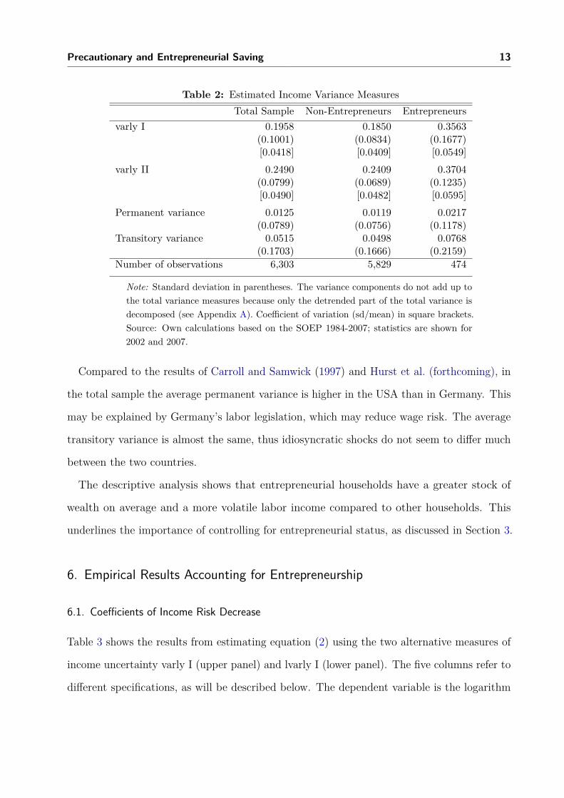
The sample means of the uncertainty measures varly I and varly II presented in Table 2
clearly confirm that entrepreneurial households face higher income risk than other house-
holds. The difference persists when the estimated variance is normalized by the mean (the
variation coefficients are reported in square brackets). When the variance is decomposed
into a permanent and a transitory component, both components turn out to be larger for
entrepreneurs.
Precautionary and Entrepreneurial Saving 13
Table 2: Estimated Income Variance MeasuresTotal Sample Non-Entrepreneurs Entrepreneurs
varly I 0.1958 0.1850 0.3563(0.1001) (0.0834) (0.1677)[0.0418] [0.0409] [0.0549]
varly II 0.2490 0.2409 0.3704(0.0799) (0.0689) (0.1235)[0.0490] [0.0482] [0.0595]
Permanent variance 0.0125 0.0119 0.0217(0.0789) (0.0756) (0.1178)
Transitory variance 0.0515 0.0498 0.0768(0.1703) (0.1666) (0.2159)
Number of observations 6,303 5,829 474
Note: Standard deviation in parentheses. The variance components do not add up tothe total variance measures because only the detrended part of the total variance isdecomposed (see Appendix A). Coefficient of variation (sd/mean) in square brackets.Source: Own calculations based on the SOEP 1984-2007; statistics are shown for2002 and 2007.
Compared to the results of Carroll and Samwick (1997) and Hurst et al. (forthcoming), in
the total sample the average permanent variance is higher in the USA than in Germany. This
may be explained by Germany’s labor legislation, which may reduce wage risk. The average
transitory variance is almost the same, thus idiosyncratic shocks do not seem to differ much
between the two countries.
The descriptive analysis shows that entrepreneurial households have a greater stock of
wealth on average and a more volatile labor income compared to other households. This
underlines the importance of controlling for entrepreneurial status, as discussed in Section 3.
6. Empirical Results Accounting for Entrepreneurship
6.1. Coefficients of Income Risk Decrease
Table 3 shows the results from estimating equation (2) using the two alternative measures of
income uncertainty varly I (upper panel) and lvarly I (lower panel). The five columns refer to
different specifications, as will be described below. The dependent variable is the logarithm
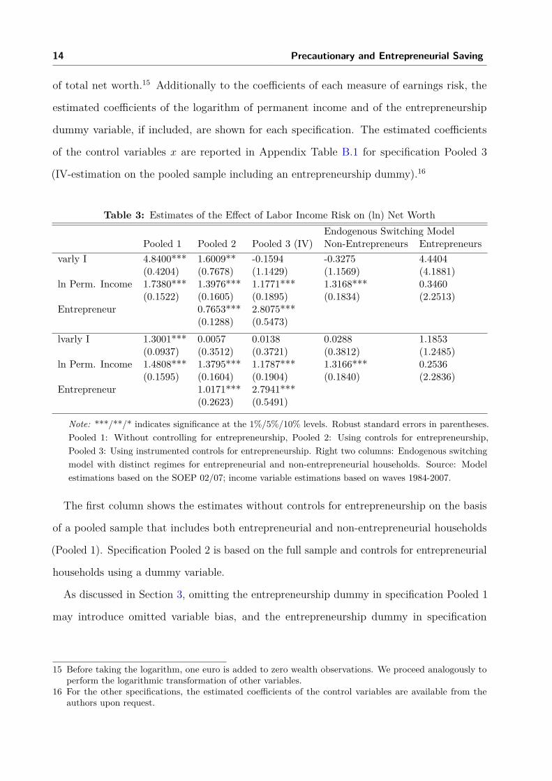
14 Precautionary and Entrepreneurial Saving
of total net worth.15 Additionally to the coefficients of each measure of earnings risk, the
estimated coefficients of the logarithm of permanent income and of the entrepreneurship
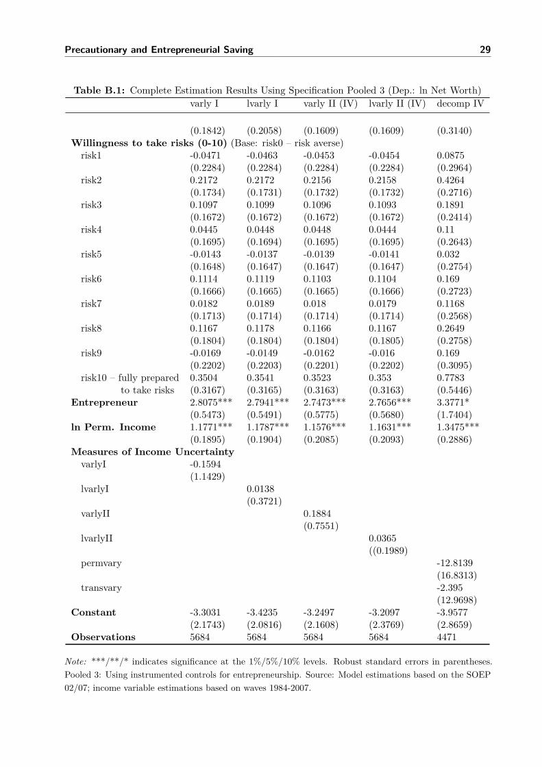
dummy variable, if included, are shown for each specification. The estimated coefficients
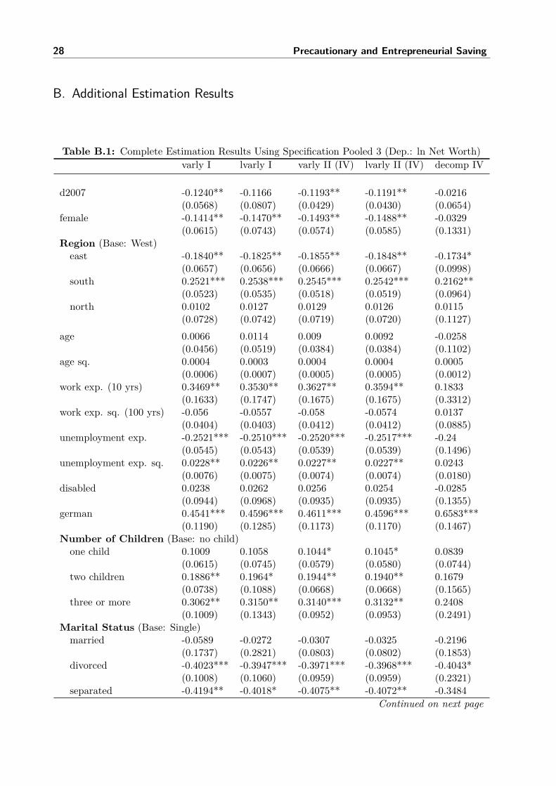
of the control variables x are reported in Appendix Table B.1 for specification Pooled 3
(IV-estimation on the pooled sample including an entrepreneurship dummy).16
Table 3: Estimates of the Effect of Labor Income Risk on (ln) Net WorthEndogenous Switching Model
Pooled 1 Pooled 2 Pooled 3 (IV) Non-Entrepreneurs Entrepreneursvarly I 4.8400*** 1.6009** -0.1594 -0.3275 4.4404
(0.4204) (0.7678) (1.1429) (1.1569) (4.1881)ln Perm. Income 1.7380*** 1.3976*** 1.1771*** 1.3168*** 0.3460
(0.1522) (0.1605) (0.1895) (0.1834) (2.2513)Entrepreneur 0.7653*** 2.8075***
(0.1288) (0.5473)lvarly I 1.3001*** 0.0057 0.0138 0.0288 1.1853
(0.0937) (0.3512) (0.3721) (0.3812) (1.2485)ln Perm. Income 1.4808*** 1.3795*** 1.1787*** 1.3166*** 0.2536
(0.1595) (0.1604) (0.1904) (0.1840) (2.2836)Entrepreneur 1.0171*** 2.7941***
(0.2623) (0.5491)
Note: ***/**/* indicates significance at the 1%/5%/10% levels. Robust standard errors in parentheses.Pooled 1: Without controlling for entrepreneurship, Pooled 2: Using controls for entrepreneurship,Pooled 3: Using instrumented controls for entrepreneurship. Right two columns: Endogenous switchingmodel with distinct regimes for entrepreneurial and non-entrepreneurial households. Source: Modelestimations based on the SOEP 02/07; income variable estimations based on waves 1984-2007.
The first column shows the estimates without controls for entrepreneurship on the basis
of a pooled sample that includes both entrepreneurial and non-entrepreneurial households
(Pooled 1). Specification Pooled 2 is based on the full sample and controls for entrepreneurial
households using a dummy variable.
As discussed in Section 3, omitting the entrepreneurship dummy in specification Pooled 1
may introduce omitted variable bias, and the entrepreneurship dummy in specification
15 Before taking the logarithm, one euro is added to zero wealth observations. We proceed analogously toperform the logarithmic transformation of other variables.
16 For the other specifications, the estimated coefficients of the control variables are available from theauthors upon request.
Precautionary and Entrepreneurial Saving 15
Pooled 2 may be endogenous. Therefore the preferred specification is the IV model Pooled 3.
As mentioned, in this specification dummy variables for a self-employed father, university
entrance qualification of the household head’s parents and his or her own educational
attainment are used as IVs for the entrepreneurship dummy.17 As the analysis of Carroll and
Samwick (1998) suggests that the logarithm of the variance of log income has a near linear
relationship with log wealth, the preferred measure of income risk is lvarly I.
The last two columns report the estimation results from the endogenous switching regression
model. The left and right columns report the estimated coefficients for the regimes faced
by non-entrepreneurial and entrepreneurial households, respectively. As mentioned, this
specification is more flexible than specification Pooled 3, as it allows the coefficients to
differ between the two household types, while accounting appropriately for endogeneity of
entrepreneurship as well.18 The disadvantage of this model is that the coefficients for the
entrepreneurs’ regime are imprecisely estimated due to the comparably small size of the
sub-sample of entrepreneurs (see Section 4).
What are the results with respect to the precautionary saving motive? In specification
Pooled 1, which does not control for entrepreneurship, the relationship between income
variance and net worth, which might be attributed to precautionary saving, is significantly
positive for both measures of income uncertainty. These results replicate the findings in the
prior literature that does not account for entrepreneurship. Looking at lvarly I, the estimated
coefficient implies that when income uncertainty doubles, total net worth increases by 130%.
Once entrepreneurship is controlled for, however, the picture changes completely. Turning to
the specifications accounting for entrepreneurship, which are found in the remaining columns
to the right, the point estimates for the income variance coefficients become substantially
17 The strength of these excluded instruments seems to be marginally sufficient. An F -test indicates thatthey are jointly significant at the 1% level (F = 9.38, if varly I is used, and F = 11.14 for lvarly I) inthe first stage regression of the entrepreneurship dummy variable on all instruments; Shea’s Partial R2
is 0.0148 (0.0146), when varly I (lvarly I) is used. The Hansen test of overidentifying restrictions is notrejected (the p-value is 0.7044 using varly I, and 0.5703 using lvarly I).
18 The variables excluded from the criterion function, which are identical to the excluded instruments inspecification Pooled 3, are jointly significant at the 1% level in the selection equation (χ2
7 = 21.04 forvarly I, χ2
7 = 20.92 for lvarly I).
16 Precautionary and Entrepreneurial Saving
smaller, in two cases even negative, regardless of whether varly I or lvarly I is used. There is
no longer a significant relationship between income uncertainty and total net worth. The
only exception to this is specification Pooled 2 using varly I, where the point estimate is also
substantially smaller than without controlling for entrepreneurship, but still significant. As
argued above, the logarithm lvarly I is the preferred measure because of the better functional
fit, however. The coefficient in the entrepreneurs’ regime of the switching regression model
is the only one that does not become substantially smaller in comparison to specification
Pooled 1. This is not inconsistent with the general result, as for this regime the estimated
coefficient has a large standard error for the reasons mentioned above, and is not significantly
different from zero. Overall the results clearly show that given the heterogeneity between
entrepreneurial and non-entrepreneurial households, not controlling for entrepreneurship
causes spurious correlation between income uncertainty and wealth and leads to an upward
bias of estimations of precautionary savings.
The estimated coefficient of the entrepreneurship dummy in the preferred specification
Pooled 3 indicates that the wealth stock held by entrepreneurial households is on average
about 15 times larger than that of a non-entrepreneurial household, holding income risk
and the other explanatory variables constant, and regardless of whether measure varly I or
lvarly I is used.19
The relationship between permanent income and total net worth is positive and significant
across all specifications and income risk measures, again except for the entrepreneurs’ regime
of the switching regression model, where the coefficient is insignificant due to a large standard
error. Focusing on specification Pooled 3 using the uncertainty measure lvarly I, the estimated
coefficient of log permanent net income implies that a doubling of permanent net income
increases total net worth by 118%.
The results remain similar when the coefficients (except for the intercept) in the endogenous
switching model are restricted to be the same in the two regimes. As mentioned in Section 3,
19 Since the dependent variable is the logarithm of total net worth, this estimate is obtained by calculatinge2.7941 − 1 = 15.35 (based on the specification using lvarly I).
Precautionary and Entrepreneurial Saving 17
this restricted model accounts for entrepreneurship by interpreting entrepreneurial status as a
treatment in the sense of a treatment effects model (Heckman, 1978). As in the other models
accounting for entrepreneurship, the coefficient of the earnings variance becomes small and
insignificant, regardless of whether varly I or lvarly I is used.20
6.2. Results Robust to Alternative Measures of Income Risk
The results from the IV estimations using the measures of income uncertainty varly II and
lvarly II and the decomposed variance are reported in Appendix Table B.2. The findings
confirm the results discussed above, which were obtained from using the variance measures
varly I and lvarly I. In specification Pooled 1 without accounting for entrepreneurship, the
estimated coefficient of earnings risk is positive and significant using all the income uncertainty
measures. Again the significance is lost and the point estimates become substantially smaller
once entrepreneurship is controlled for by including an entrepreneurship dummy assumed to
be exogenous (Pooled 2) or endogenous (Pooled 3, using the same additional instruments as
before).
The Hansen test of overidentifying restrictions does not indicate invalidity of the instru-
mental variables.21 The instruments seem to be sufficiently strong for the income risk
measures varly II and lvarly II, as Shea’s Partial R2 is 0.17 and 0.21, respectively. For the
entrepreneurship indicator, Shea’s Partial R2 is only 0.017 using both variance measures. A
likely reason for the higher correlation of the instruments with the variance measures is that
the educational dummy variables used as IVs are also used to define cells for the construction
of these variance measures, so the indicator may not be very informative. The strength of
the instruments for the decomposed variance measure is clearly non-satisfying, as indicated
by a Partial R2 of 0.0017 for the variance of permanent shocks and 0.0008 for the variance
20 The results are available from the authors upon request. In this paper we report the results of the moregeneral endogenous switching model only, because the restrictions of equal coefficients in the two regimesare rejected by an LR test (χ2
32 = 111.32 using lvarly I). The treatment effects model is similar to theIV model Pooled 3, which we prefer, because the former model requires the assumption of normallydistributed error terms for consistency.
21 The p-value of this test is 0.5817 (0.5769) using varly II (lvarly II) and 0.3965 for the decomposed variancemeasures.
18 Precautionary and Entrepreneurial Saving
of transitory shocks. Hurst et al. (forthcoming) reported similar weak instrument problems.
The results based on these variance measures must thus be interpreted with caution; this is
the main reason why we prefer the measures varly I and lvarly I.
6.3. Share of Precautionary Savings in Total Net Worth Becomes Small
To quantify the amount of precautionary savings based on the estimated parameters, we
follow the literature and compare the predicted net worth of households Wi with the simulated
net worth they would hold if they all faced the minimum income risk. The minimum income
risk ω∗ is approximated by the minimum predicted risk in the sample. A prediction of W ∗i ,
obtained by substituting the households’ income risk ωi by ω∗, can be interpreted as the
amount that households would accumulate if they faced the minimum risk. The share of
total net worth explained by precautionary saving in the sample is then given by
∑Ni=1 Wi −
∑Ni=1 W
∗i∑N
i=1 Wi
. (6)
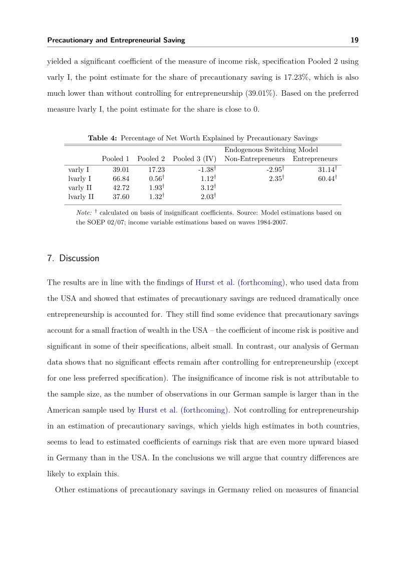
Table 4 shows the estimated share of precautionary savings in total net worth, based on the
different specifications and measures of income risk. Without controlling for entrepreneurship
(Pooled 1), the estimated amount of precautionary savings is large, which replicates results
reported in the literature (Carroll and Samwick, 1998). Using the preferred measure lvarly I,
it even accounts for 66.84% of total net worth. Once entrepreneurship is controlled for by
including a dummy or applying the switching regression model, the point estimates of the
shares become substantially smaller (and even slightly negative in two specifications), except
for the entrepreneurs’ regime in the switching regression model. Even in this regime, the
hypothesis that precautionary savings are zero cannot be rejected, because the coefficients of
the income variance are insignificant, as in almost all the other specifications accounting for
entrepreneurship.22 Based on the only specification controlling for entrepreneurship which
22 This is also true for the decomposed variance measure. For this measure, the share of precautionarysavings is not reported in the table, because the coefficients are too imprecisely estimated and potentiallybiased due to weak instruments, as mentioned above.
Precautionary and Entrepreneurial Saving 19
yielded a significant coefficient of the measure of income risk, specification Pooled 2 using
varly I, the point estimate for the share of precautionary saving is 17.23%, which is also
much lower than without controlling for entrepreneurship (39.01%). Based on the preferred
measure lvarly I, the point estimate for the share is close to 0.
Table 4: Percentage of Net Worth Explained by Precautionary SavingsEndogenous Switching Model
Pooled 1 Pooled 2 Pooled 3 (IV) Non-Entrepreneurs Entrepreneursvarly I 39.01 17.23 -1.38† -2.95† 31.14†lvarly I 66.84 0.56† 1.12† 2.35† 60.44†varly II 42.72 1.93† 3.12†lvarly II 37.60 1.32† 2.03†
Note: † calculated on basis of insignificant coefficients. Source: Model estimations based onthe SOEP 02/07; income variable estimations based on waves 1984-2007.
7. Discussion
The results are in line with the findings of Hurst et al. (forthcoming), who used data from
the USA and showed that estimates of precautionary savings are reduced dramatically once
entrepreneurship is accounted for. They still find some evidence that precautionary savings
account for a small fraction of wealth in the USA – the coefficient of income risk is positive and
significant in some of their specifications, albeit small. In contrast, our analysis of German
data shows that no significant effects remain after controlling for entrepreneurship (except
for one less preferred specification). The insignificance of income risk is not attributable to
the sample size, as the number of observations in our German sample is larger than in the
American sample used by Hurst et al. (forthcoming). Not controlling for entrepreneurship
in an estimation of precautionary savings, which yields high estimates in both countries,
seems to lead to estimated coefficients of earnings risk that are even more upward biased
in Germany than in the USA. In the conclusions we will argue that country differences are
likely to explain this.
Other estimations of precautionary savings in Germany relied on measures of financial
20 Precautionary and Entrepreneurial Saving
wealth instead of total net worth as the dependent variable. Specifically, Fuchs-Schündeln
and Schündeln (2005) and Bartzsch (2008) estimated the amount of precautionary savings to
be about 20% after employing different strategies to control for heterogeneity in risk aversion.
As they excluded the self-employed, they avoided the spurious correlation problem arising
from pooling non-entrepreneurial and entrepreneurial households without controlling for
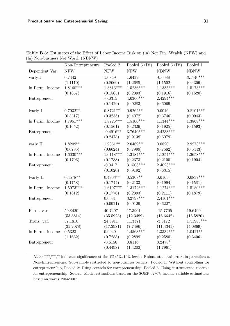
entrepreneurship. To allow for a comparison, Table B.3 in the Appendix shows estimation
results using net financial wealth as the dependent variable. The leftmost column presents
results from a sample excluding entrepreneurs, similarly to the two studies mentioned. Using
lvarly II as the measure of income risk, which is very similar to one of the measures used
in the two studies mentioned, the coefficient of income risk turns out to be positive and
significant, which replicates the general results of the two studies. Positive and significant
results are also obtained using the preferred specification Pooled 3 (IV-estimation based on
the pooled sample with an endogenous entrepreneurship dummy), based on all measures of
income risk except for varly I and the decomposed variance measure. The positive effect thus
seems to arise when financial wealth is chosen as the dependent variable.
These findings show that households with higher income risk hold more liquid financial
wealth such as cash, bonds and shares. Interpreting this as evidence for precautionary saving
is problematic, however. Given that the results from using total net worth as the dependent
variable indicated that total net worth does not react significantly upon changes in income
risk, the changes in financial assets must rather be interpreted as portfolio decisions. The
larger amount of financial assets that households with higher income risk hold must be offset
by a smaller amount in other assets such as property, holding total net worth constant. It
seems plausible that households with more volatile income hold a larger share of their wealth
in liquid assets. In the light of the findings from this study, this does not mean that these
households save more, however.
As an additional robustness test, total net worth minus the value of a private business is
used as the dependent variable. The second column from the right in Table B.3 shows results
obtained from substituting the dependent variable in the preferred specification Pooled 3. The
Precautionary and Entrepreneurial Saving 21
effect of controlling for entrepreneurship does not change: Regardless of the measure of income
variance used, the estimated coefficients of income risk are small and insignificant. In the
rightmost column of the table, the modified dependent variable is plugged into specification
Pooled 1, which does not include an entrepreneurship dummy variable. Here, the estimated
coefficients of income risk are smaller than those obtained when total net worth is used as
the dependent variable in the same specification, but they are still positive and significant. If
the only channel for entrepreneurs’ additional saving were investment in their own business,
removing business wealth from the wealth measure would be sufficient to avoid the upward
bias in the coefficient of earnings risk that results from not accounting for entrepreneurship.
The results from this last test show that this does not seem to be true, at least in Germany,
and invalidate the approach referred to as potential strategy 3 in Section 3. It is very plausible
that additional savings of entrepreneurs that are unrelated to the precautionary motive,
e.g. savings for old age consumption in order to make up for the lack of statutory pension
insurance, are not exclusively concentrated in their business, but also in other assets such as
property and private pension insurance.
8. Conclusion
Empirical estimates of large amounts of precautionary savings disappear once the heterogeneity
between entrepreneurial and non-entrepreneurial households is accounted for, as reported
by Hurst et al. (forthcoming) using data from the USA. This paper is the first to confirm
the result in a different country by revising estimates of precautionary savings in Germany.
While Hurst et al. (forthcoming) still find some evidence that precautionary savings account
for a small fraction of wealth in the USA, the results from this study based on the preferred
specifications actually show that no significant estimates of precautionary savings remain in
Germany once entrepreneurship is controlled for.
Hence, not controlling for entrepreneurship in an estimation of precautionary savings, which
yields high estimates in both countries, is even more misleading in Germany than in the USA.
A possible explanation is that the difference in the saving behavior between entrepreneurial
22 Precautionary and Entrepreneurial Saving
and non-entrepreneurial households is even more pronounced in countries with an extensive
social security system such as Germany than in a country following the Anglo-Saxon model.
In Germany, employees are covered by statutory pension insurance, while entrepreneurs
have to save for their old age consumption. Thus, the extra saving of entrepreneurs is
likely to be due to their exclusion from the social security system. Pooling together the two
household types without controlling for entrepreneurship misleadingly connects the higher
savings of entrepreneurs to their higher income risk and leads to an upward bias in estimates
of precautionary savings.
Prior studies which estimated precautionary savings in Germany, particularly Fuchs-
Schündeln and Schündeln (2005) and Bartzsch (2008), analyzed the effect of income risk on
certain components of wealth such as net financial wealth. They interpreted their results as
evidence for precautionary savings. While these results can be replicated, in this paper it is
shown that there are no significant effects of income risk on total net worth. Thus, higher
income risk seems to be associated with a portfolio shift towards more liquid assets, but not
with more saving.
Methodologically, the main innovation in this study is that entrepreneurship is recognized as
being endogenous with wealth, as suggested by the large literature on credit constraints faced
by nascent entrepreneurs. This study employs IV estimators and an endogenous switching
regression model, where entrepreneurial and non-entrepreneurial households face different
regimes, to deal with this endogeneity.
Estimates of precautionary saving are important for policy design, especially labor market,
social security, and taxation policy, as these policies directly affect the variance of households’
net income. Governments in Western welfare states have tended to downsize the social
security system during the last decades. At the same time, collective labor agreements have
lost importance in some countries such as Germany. Prior estimates of precautionary saving
suggested that households would considerably increase their savings due to the rising income
uncertainty. In contrast, the new findings in this study, which account for the important role
of entrepreneurship, imply that no significant effects on the savings rate are to be expected.
Precautionary and Entrepreneurial Saving 23
References
Bartzsch, N. (2008): “Precautionary Saving and Income Uncertainty in Germany - New
Evidence from Microdata,” Journal of Economics and Statistics (Jahrbuecher fuer Nation-
aloekonomie und Statistik), 228(1), 5–24.
Blanchflower, D. G., and A. J. Oswald (1998): “What Makes an Entrepreneur?,”
Journal of Labor Economics, 16(1), 26–60.
Carroll, C. D. (1992): “The Buffer-Stock Theory of Saving: Some Macroeconomic
Evidence,” Brookings Papers on Economic Activity, 23(1992-2), 61–156.
(1997): “Buffer-Stock Saving and the Life Cycle/Permanent Income Hypothesis,”
Quarterly Journal of Economics, 112(1), 1–55.
(2004): “Theoretical Foundations of Buffer Stock Saving,” Economics Working
Paper Archive 517, The Johns Hopkins University, Department of Economics.
Carroll, C. D., and A. A. Samwick (1997): “The Nature of Precautionary Wealth,”
Journal of Monetary Economics, 40(1), 41–71.
(1998): “How Important Is Precautionary Saving?,” Review of Economics and
Statistics, 80(3), 410–419.
Deaton, A. (1991): “Saving and Liquidity Constraints,” Econometrica, 59(5), 1221–48.
Deutsche Rentenversicherung (2007): Jahresbericht 2007, available at
http://www.deutsche-rentenversicherung.de/.
Dohmen, T., A. Falk, D. Huffman, U. Sunde, J. Schupp, and G. G. Wagner (2005):
“Individual Risk Attitudes : New Evidence from a Large, Representative, Experimentally-
Validated Survey,” Discussion Papers of DIW Berlin 511, German Institute for Economic
Research.
24 Precautionary and Entrepreneurial Saving
Dunn, T., and D. Holtz-Eakin (2000): “Financial Capital, Human Capital, and the
Transition to Self-Employment: Evidence from Intergenerational Links,” Journal of Labor
Economics, 18(2), 282–305.
Engen, E. M., and J. Gruber (2001): “Unemployment Insurance and Precautionary
Saving,” Journal of Monetary Economics, 47(3), 545 – 579.
Essig, L. (2005): “Precautionary Saving and Old-Age Provisions: Do Subjective Saving
Motive Measures Work?,” MEA discussion paper series 05084, Mannheim Research Institute
for the Economics of Aging (MEA), University of Mannheim.
Femminis, G. (2001): “Risk-Sharing and Growth: The Role of Precautionary Savings in the
"Education" Model,” Scandinavian Journal of Economics, 103(1), 63–77.
Fossen, F. M. (2008): “The Private Equity Premium Puzzle Revisited: New Evidence on
the Role of Heterogeneous Risk Attitudes,” Discussion Papers of DIW Berlin 839, German
Institute for Economic Research.
Fuchs-Schündeln, N., and M. Schündeln (2005): “Precautionary Savings and Self-
Selection: Evidence from the German Reunification "Experiment",” Quarterly Journal of
Economics, 120, 1085–1120.
Heckman, J. J. (1978): “Dummy Endogenous Variables in a Simultaneous Equation System,”
Econometrica, 46(4), 931–959.
Hurst, E., A. Kennickell, A. Lusardi, and F. Torralba (forthcoming, available
at http://faculty.chicagogsb.edu/erik.hurst/research/ ): “Precautionary Savings and the
Importance of Business Owners,” Review of Economics and Statistics.
Hurst, E., and A. Lusardi (2004): “Liquidity Constraints, Household Wealth, and
Entrepreneurship,” Journal of Political Economy, 112(2), 319–347.
Johansson, E. (2000): “Self-Employment and Liquidity Constraints: Evidence from Fin-
land,” Scandinavian Journal of Economics, 102(1), 123–34.
Precautionary and Entrepreneurial Saving 25
Kazarosian, M. (1997): “Precautionary Savings-A Panel Study,” The Review of Economics
and Statistics, 79(2), 241–247.
Lokshin, M., and Z. Sajaia (2004): “Maximum Likelihood Estimation of Endogenous
Switching Regression Models,” Stata Journal, 4(3), 282–289.
Lusardi, A. (1997): “Precautionary Saving and Subjective Earnings Variance,” Economics
Letters, 57(3), 319–326.
(1998): “On the Importance of the Precautionary Saving Motive,” American
Economic Review, 88(2), 449–53.
Maddala, G. S. (1983): Limited-Dependent and Qualitative Variables in Econometrics.
Cambridge: Cambridge University Press.
Nykvist, J. (2008): “Entrepreneurship and Liquidity Constraints: Evidence from Sweden,”
Scandinavian Journal of Economics, 110(1), 23–43.
Schunk, D. (2007): “What Determines the Saving Behavior of German Households? An
Examination of Saving Motives and Saving Decisions,” MEA discussion paper series 07124,
Mannheim Research Institute for the Economics of Aging (MEA), University of Mannheim.
Wagner, G. G., J. R. Frick, and J. Schupp (2007): “The German Socio-Economic
Panel Study (SOEP): Scope, Evolution and Enhancements,” Journal of Applied Social
Science Studies, 127(1), 139–169.
26 Precautionary and Entrepreneurial Saving
Appendix
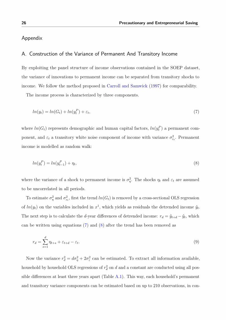
A. Construction of the Variance of Permanent And Transitory Income
By exploiting the panel structure of income observations contained in the SOEP dataset,
the variance of innovations to permanent income can be separated from transitory shocks to
income. We follow the method proposed in Carroll and Samwick (1997) for comparability.
The income process is characterized by three components.
ln(yt) = ln(Gt) + ln(yPt ) + εt, (7)
where ln(Gt) represents demographic and human capital factors, ln(yPt ) a permanent com-
ponent, and εt a transitory white noise component of income with variance σ2εt . Permanent
income is modelled as random walk:
ln(yPt ) = ln(yPt−1) + ηt, (8)
where the variance of a shock to permanent income is σ2η. The shocks ηt and εt are assumed
to be uncorrelated in all periods.
To estimate σ2η and σ2
εt , first the trend ln(Gt) is removed by a cross-sectional OLS regression
of ln(yt) on the variables included in x1, which yields as residuals the detrended income yt.
The next step is to calculate the d-year differences of detrended income: rd = yt+d− yt, which
can be written using equations (7) and (8) after the trend has been removed as
rd =d∑s=1
ηt+s + εt+d − εt. (9)
Now the variance r2d = dσ2
η + 2σ2ε can be estimated. To extract all information available,
household by household OLS regressions of r2d on d and a constant are conducted using all pos-
sible differences at least three years apart (Table A.1). This way, each household’s permanent
and transitory variance components can be estimated based on up to 210 observations, in con-

Precautionary and Entrepreneurial Saving 27
Table A.1: Observations used to esti-mate households variances
d=3 d=4 · · · d=231987-1984 1988-1984 · · · 2007-19841988-1985 1989-1985
......
2006-2003 2007-20032007-2004
20 19 · · · 1
trast to only nine observations in Carroll and Samwick (1997) and Hurst et al. (forthcoming).
Households for which only 3 or less observations are available are not considered.
28 Precautionary and Entrepreneurial Saving
B. Additional Estimation Results
Table B.1: Complete Estimation Results Using Specification Pooled 3 (Dep.: ln Net Worth)varly I lvarly I varly II (IV) lvarly II (IV) decomp IV
d2007 -0.1240** -0.1166 -0.1193** -0.1191** -0.0216(0.0568) (0.0807) (0.0429) (0.0430) (0.0654)
female -0.1414** -0.1470** -0.1493** -0.1488** -0.0329(0.0615) (0.0743) (0.0574) (0.0585) (0.1331)
Region (Base: West)east -0.1840** -0.1825** -0.1855** -0.1848** -0.1734*
(0.0657) (0.0656) (0.0666) (0.0667) (0.0998)south 0.2521*** 0.2538*** 0.2545*** 0.2542*** 0.2162**
(0.0523) (0.0535) (0.0518) (0.0519) (0.0964)north 0.0102 0.0127 0.0129 0.0126 0.0115
(0.0728) (0.0742) (0.0719) (0.0720) (0.1127)age 0.0066 0.0114 0.009 0.0092 -0.0258
(0.0456) (0.0519) (0.0384) (0.0384) (0.1102)age sq. 0.0004 0.0003 0.0004 0.0004 0.0005
(0.0006) (0.0007) (0.0005) (0.0005) (0.0012)work exp. (10 yrs) 0.3469** 0.3530** 0.3627** 0.3594** 0.1833
(0.1633) (0.1747) (0.1675) (0.1675) (0.3312)work exp. sq. (100 yrs) -0.056 -0.0557 -0.058 -0.0574 0.0137
(0.0404) (0.0403) (0.0412) (0.0412) (0.0885)unemployment exp. -0.2521*** -0.2510*** -0.2520*** -0.2517*** -0.24
(0.0545) (0.0543) (0.0539) (0.0539) (0.1496)unemployment exp. sq. 0.0228** 0.0226** 0.0227** 0.0227** 0.0243
(0.0076) (0.0075) (0.0074) (0.0074) (0.0180)disabled 0.0238 0.0262 0.0256 0.0254 -0.0285
(0.0944) (0.0968) (0.0935) (0.0935) (0.1355)german 0.4541*** 0.4596*** 0.4611*** 0.4596*** 0.6583***
(0.1190) (0.1285) (0.1173) (0.1170) (0.1467)Number of Children (Base: no child)
one child 0.1009 0.1058 0.1044* 0.1045* 0.0839(0.0615) (0.0745) (0.0579) (0.0580) (0.0744)
two children 0.1886** 0.1964* 0.1944** 0.1940** 0.1679(0.0738) (0.1088) (0.0668) (0.0668) (0.1565)
three or more 0.3062** 0.3150** 0.3140*** 0.3132** 0.2408(0.1009) (0.1343) (0.0952) (0.0953) (0.2491)
Marital Status (Base: Single)married -0.0589 -0.0272 -0.0307 -0.0325 -0.2196
(0.1737) (0.2821) (0.0803) (0.0802) (0.1853)divorced -0.4023*** -0.3947*** -0.3971*** -0.3968*** -0.4043*
(0.1008) (0.1060) (0.0959) (0.0959) (0.2321)separated -0.4194** -0.4018* -0.4075** -0.4072** -0.3484
Continued on next page
Precautionary and Entrepreneurial Saving 29
Table B.1: Complete Estimation Results Using Specification Pooled 3 (Dep.: ln Net Worth)varly I lvarly I varly II (IV) lvarly II (IV) decomp IV
(0.1842) (0.2058) (0.1609) (0.1609) (0.3140)Willingness to take risks (0-10) (Base: risk0 – risk averse)
risk1 -0.0471 -0.0463 -0.0453 -0.0454 0.0875(0.2284) (0.2284) (0.2284) (0.2284) (0.2964)
risk2 0.2172 0.2172 0.2156 0.2158 0.4264(0.1734) (0.1731) (0.1732) (0.1732) (0.2716)
risk3 0.1097 0.1099 0.1096 0.1093 0.1891(0.1672) (0.1672) (0.1672) (0.1672) (0.2414)
risk4 0.0445 0.0448 0.0448 0.0444 0.11(0.1695) (0.1694) (0.1695) (0.1695) (0.2643)
risk5 -0.0143 -0.0137 -0.0139 -0.0141 0.032(0.1648) (0.1647) (0.1647) (0.1647) (0.2754)
risk6 0.1114 0.1119 0.1103 0.1104 0.169(0.1666) (0.1665) (0.1665) (0.1666) (0.2723)
risk7 0.0182 0.0189 0.018 0.0179 0.1168(0.1713) (0.1714) (0.1714) (0.1714) (0.2568)
risk8 0.1167 0.1178 0.1166 0.1167 0.2649(0.1804) (0.1804) (0.1804) (0.1805) (0.2758)
risk9 -0.0169 -0.0149 -0.0162 -0.016 0.169(0.2202) (0.2203) (0.2201) (0.2202) (0.3095)
risk10 – fully prepared 0.3504 0.3541 0.3523 0.353 0.7783to take risks (0.3167) (0.3165) (0.3163) (0.3163) (0.5446)
Entrepreneur 2.8075*** 2.7941*** 2.7473*** 2.7656*** 3.3771*(0.5473) (0.5491) (0.5775) (0.5680) (1.7404)
ln Perm. Income 1.1771*** 1.1787*** 1.1576*** 1.1631*** 1.3475***(0.1895) (0.1904) (0.2085) (0.2093) (0.2886)
Measures of Income UncertaintyvarlyI -0.1594
(1.1429)lvarlyI 0.0138
(0.3721)varlyII 0.1884
(0.7551)lvarlyII 0.0365
((0.1989)permvary -12.8139
(16.8313)transvary -2.395
(12.9698)Constant -3.3031 -3.4235 -3.2497 -3.2097 -3.9577
(2.1743) (2.0816) (2.1608) (2.3769) (2.8659)Observations 5684 5684 5684 5684 4471
Note: ***/**/* indicates significance at the 1%/5%/10% levels. Robust standard errors in parentheses.Pooled 3: Using instrumented controls for entrepreneurship. Source: Model estimations based on the SOEP02/07; income variable estimations based on waves 1984-2007.

30 Precautionary and Entrepreneurial Saving
Table B.2: IV-Estimates of the Effect of Labor Income Risk on (ln) NetWorth
Pooled 1 Pooled 2 Pooled 3varly II 4.9050*** 0.1700 0.1884
(0.5552) (0.7185) (0.7551)ln Perm. Income 1.4162*** 1.3560*** 1.1576***
(0.1958) (0.1892) (0.2085)Entrepreneur 1.0060*** 2.7473***
(0.0945) (0.5775)lvarly II 1.1701*** 0.0314 0.0365
(0.1605) (0.1879) (0.1989)ln Perm. Income 1.6647*** 1.3634*** 1.1631***
(0.1921) (0.1879) (0.2093)Entrepreneur 1.0132*** 2.7656***
(0.0843) (0.5680)Perm. var. 33.4779* 3.3450 -12.8139
(20.0179) (30.4036) (16.8313)Trans. var. 31.0954*** 11.5044 -2.3950
(6.6433) (18.3140) (12.9698)ln Perm. Income 0.7025 1.1948** 1.3475***
(0.4896) (0.5565) (0.2886)Entrepreneur 0.6018 3.3771*
(0.5434) (1.7404)
Note: ***/**/* indicates significance at the 1%/5%/10% levels. Robust standarderrors in parentheses. Pooled 1: Without controlling for entrepreneurship,Pooled 2: Using controls for entrepreneurship, Pooled 3: Using instrumentedcontrols for entrepreneurship. Source: Model estimations based on the SOEP02/07; income variable estimations based on waves 1984-2007.
Precautionary and Entrepreneurial Saving 31
Table B.3: Estimates of the Effect of Labor Income Risk on (ln) Net Fin. Wealth (NFW) and(ln) Non-business Net Worth (NBNW)
Non-Entrepreneurs Pooled 2 Pooled 3 (IV) Pooled 3 (IV) Pooled 1Dependent Var. NFW NFW NFW NBNW NBNWvarly I 0.7442 1.0849 1.6439 -0.0688 3.1740***
(1.1110) (0.8069) (1.2685) (1.1502) (0.4309)ln Perm. Income 1.8160*** 1.8816*** 1.5236*** 1.1335*** 1.5178***
(0.1657) (0.1565) (0.2393) (0.1916) (0.1520)Entrepreneur -0.0315 4.0360*** 2.4294***
(0.1429) (0.9283) (0.6069)lvarly I 0.7932** 0.8721** 0.9262** 0.0016 0.8101***
(0.3317) (0.3235) (0.4072) (0.3746) (0.0943)ln Perm. Income 1.7951*** 1.8725*** 1.5100*** 1.1344*** 1.3868***
(0.1652) (0.1561) (0.2329) (0.1925) (0.1593)Entrepreneur -0.4916** 3.7640*** 2.4233***
(0.2478) (0.9138) (0.6079)varly II 1.8209** 1.9061** 2.0469** 0.0820 2.9273***
(0.6785) (0.6624) (0.7999) (0.7582) (0.5443)ln Perm. Income 1.6030*** 1.6118*** 1.3184*** 1.1254*** 1.3658***
(0.1796) (0.1788) (0.2373) (0.2100) (0.1904)Entrepreneur -0.0417 3.1503*** 2.4023***
(0.1020) (0.9192) (0.6315)lvarly II 0.4578** 0.4963** 0.5308** 0.0163 0.6837***
(0.1758) (0.1744) (0.2133) (0.1994) (0.1581)ln Perm. Income 1.5973*** 1.6197*** 1.3172*** 1.1274*** 1.5180***
(0.1812) (0.1776) (0.2393) (0.2111) (0.1879)Entrepreneur 0.0081 3.2798*** 2.4101***
(0.0921) (0.9129) (0.6227)Perm. var. 59.8420 40.7497 17.3901 -15.7705 19.6490
(53.8814) (35.5923) (12.3489) (16.6642) (16.5820)Trans. var. 37.1810 24.8911 11.3371 -3.8172 17.1983***
(25.2078) (17.2981) (7.7486) (11.4341) (4.0869)ln Perm. Income 0.5323 0.9949 1.4563*** 1.3332*** 1.0427**
(1.1632) (0.7288) (0.2899) (0.2580) (0.3406)Entrepreneur -0.6156 0.8116 3.2478*
(0.4498) (1.4202) (1.7961)
Note: ***/**/* indicates significance at the 1%/5%/10% levels. Robust standard errors in parentheses.Non-Entrepreneurs: Sub-sample restricted to non-business owners. Pooled 1: Without controlling forentrepreneurship, Pooled 2: Using controls for entrepreneurship, Pooled 3: Using instrumented controlsfor entrepreneurship. Source: Model estimations based on the SOEP 02/07; income variable estimationsbased on waves 1984-2007.