on optimal disc covers and a new characterization of the ... · i=1 s p i (), arose in the analysis...

On Optimal Disc Covers and

a New Characterization of the Steiner Center

Yael Yankelevsky and Alfred M. Bruckstein

Technion - Israel Institute of TechnologyHaifa 32000, Israel

September 23, 2013

Abstract

Given N points in the plane P1, P2, ..., PN and a location Ω, the unionof discs with diameters [ΩPi], i = 1, 2, ..., N covers the convex hull of thepoints.

The location Ωs minimizing the area covered by the union of discs, isshown to be the Steiner center of the convex hull of the points. Similarresults for d-dimensional Euclidean space are discussed.

1 Introduction

In this paper we discuss a sphere coverage problem and, in this context, wepropose an optimal coverage criterion defining a center for a given set of pointsin space.

Suppose that a constellation of N points P1, P2, ..., PN in Rd (the d-dimensional Euclidean space) is given. An arbitrary point Ω ∈ Rd is selected andthe spheres SPi(Ω), having [ΩPi] as diameters, are defined. Hence the centersof SPi

(Ω) are at 12 (Ω + Pi) and their radii are 1

2‖Ω− Pi‖, ∀i = 1, 2, ..., N .Consider the union of these spheres SPi

(Ω), their surface ”anchored” at Ω.First we prove that the resulting d-dimensional shape always covers the convexhull of the given points P1, P2, ..., PN , hence its volume exceeds the volume ofCH P1, P2, ..., PN for all Ω ∈ Rd. This leads to the following natural question:what is the location Ω∗ which minimizes the excess (or overflow) volume and

hence the total volume of the shape, Σ(Ω) =⋃Ni=1 SPi

(Ω)?Such a location, we claim, would be a natural candidate as a ”center” for

the constellation of points P1, P2, ..., PN.The problem of determining the point that gives the tightest cover with

spheres, minimizing the excess volume beyond the convex hull, is solved herefor the planar case (i.e. d = 2). The result is the following: the optimallocation Ω∗, is the so called Steiner center of the convex hull of the given

1

Technion - Computer Science Department - Technical Report CIS-2013-01 - 2013

points P1, P2, ..., PN ∈ R2. Hence, the Steiner center Ωs of a convex poly-gon [V1V2...Vk] is also characterized as the point that yields the tightest disccover with discs having [ΩsVj ] as diameters (j = 1, 2, ...k).

For the d-dimensional case we conjecture that a similar result holds, howeverwe have no proof (yet) for this.

Finding meaningful centers for a collection of data points is a fundamentalgeometric problem in various data analysis and operation research/facility lo-cation applications. The Steiner center, along with the center of gravity, thecentroid of the convex hull and the Weber-Fermat median, were all subject tointense research (see e.g. [5],[2],[3],[1],[7],[12]). All these points are character-ized by various optimization criteria, such as (weighted) sums of distances (orfunctions of distances) to the given points. Minimax criteria, such as locationsminimizing the maximal distance to a set of given points, with various metricsyielding so called δ-centers, among them the center of the smallest coveringsphere, as optimal centers for point constellations were also subject to extensiveinvestigations over the years.

However, we have never encountered a ”center” location optimization crite-rion expressed as the area of a union of shapes defined in terms of the variablepoint Ω and the points of the given data set. We note that the problem of cover-ing the convex hull of a set of points with unions of spheres, Σ(Ω) =

⋃Ni=1 SPi

(Ω),arose in the analysis of monitoring threshold functions over distributed datastreams, in the work of Sharfman, Schuster and Keren [10]. They provide aproof of the coverage result based on a variant of Caratheodory’s theorem, us-ing induction on the dimensionality d. Our proof is simpler and direct, and doesnot rely on any results beyond the definition of convexity.

The rest of the paper is organized as follows: Section 2 proves the theoremon coverage of the convex hull in Rd, then Section 3 analyzes the problem forthe plane (d = 2) and presents an even simpler argument proving convex hullcoverage and shows that the optimal Ω is the Steiner point of the convex hull ofa planar constellation of points. In Section 4 we follow with a discussion on theSteiner point and its other nice properties and provide some numerical evidencethat the Steiner center is also optimally tight in covering the convex hull of thedata points in 3-dimensions. Finally, Section 5 offers some concluding remarks.

2 d-dimensional sphere covers

Given a set of points in Rd, denoted by P1, P2, ..., PN, for any Ω ∈ Rd definethe spheres SPi

(Ω) with center at the midpoint of the segment [ΩPi] and radius12‖ΩPi‖. We prove the following:

Theorem 1.

CH P1, P2, ..., PN ⊂N⋃i=1

SPi(Ω) (1)

2


where CH P1, P2, ..., PN denotes the convex hull of the points P1, P2, ..., PN .

Without loss of generality, we choose the coordinate system such that Ω isthe origin, i.e. Ω = (0, 0, ...0) ∈ Rd. Denote a general point in the convex hull

of P1, P2, ..., PN by Q =∑Ni=1 λiPi (with λi ≥ 0,

∑Ni=1 λi = 1) .

To prove the inclusion of the convex hull in the union of the spheres SPi(Ω)

we must show that:

∃i ∈ 1, 2, ..., N s.t. d(Q,1

2Pi) ≤ d(Ω,

1

2Pi) (2)

hence Q is inside at least one of the spheres, being closer to the sphere centerthan its radius. This clearly implies that:

Q ∈ CH P1, P2, ..., PN ⇒ Q ∈N⋃i=1

SPi(Ω) (3)

Proof of Theorem 1. Assume that

d(Q,1

2Pi) > d(Ω,

1

2Pi) ∀i ∈ 1, 2, ..., N (4)

Hence we have

d2(Q,1

2Pi) > d2(Ω,

1

2Pi)

(Q− 1

2Pi)

T (Q− 1

2Pi) >

1

2PTi ·

1

2Pi

QTQ−QTPi > 0

QT (Pi −Q) < 0 ∀i ∈ 1, 2, ..., N (5)

This means that the projections of all the vectors from Q to Pi (= ~Pi− ~Q), on

the vector from Ω to Q (= ~Q) are strictly negative (see Figure 1). But this is im-possible since Q ∈ CHP1, P2, ..., PN and this implies that CHP1, P2, ..., PNcannot project on the line ΩQ on ”one side” of Q.

Figure 1: Strictly negative projections

3


The contradiction to the assumption in (4) proves that we must have forsome i:

d(Q,1

2Pi) ≤ d(Ω,

1

2Pi) (6)

Hence

Q ∈ CH P1, P2, ..., PN ⇒ Q ∈N⋃i=1

SPi(Ω) (7)

As stated in the introduction, Theorem 1 is due to D. Keren and his cowork-ers (see [10],[6]). Their proof is rather complex, being based on Caratheodory’stheorem on convex sets and induction on the dimensionality d.

Since CH P1, P2, ..., PN ⊂⋃Ni=1 SPi

(Ω) , we have that

V olume

(N⋃i=1

SPi(Ω)

)= V olume (CH P1, ..., PN)

+V olume

(N⋃i=1

SPi(Ω) \ CH P1, P2, ..., PN

)

It therefore makes sense to ask what is the location Ω∗ that minimizes thevolume of the union of spheres SPi

(Ω), hence also the excess volume beyond theconvex hull of the data points. In the next section we solve this problem forthe important planar case. Surprisingly, the optimal location turns out to be awell-known center for planar convex shapes.

3 A discovery on disc covers

In this section, we analyze the planar disc covering problem, first providing aneven simpler proof of the convex hull coverage result and then determining thelocation of Ω that results in the tightest cover.Given N points in the plane, R2, we shall prove that:

1. The discs SPi(Ω) cover their convex hull,

2. The optimal location for Ω∗, yielding the tightest cover, is the Steinercenter of the convex hull polygon.

The second result provides a novel characterization for the Steiner point ofa convex polygon in the plane, namely:

Given V1, V2, ..., Vk the vertices of a convex polygon in R2, the Steinerpoint Ωs is the solution of

Ωs = arg minΩ

Area

(k⋃i=1

SVi(Ω)

)(8)

4


A traditional characterization of the Steiner point is

Ωs = arg minΩ

k∑i=1

θid2(Vi,Ω) (9)

yielding explicitly

Ωs =1

2π

k∑i=1

θiVi (10)

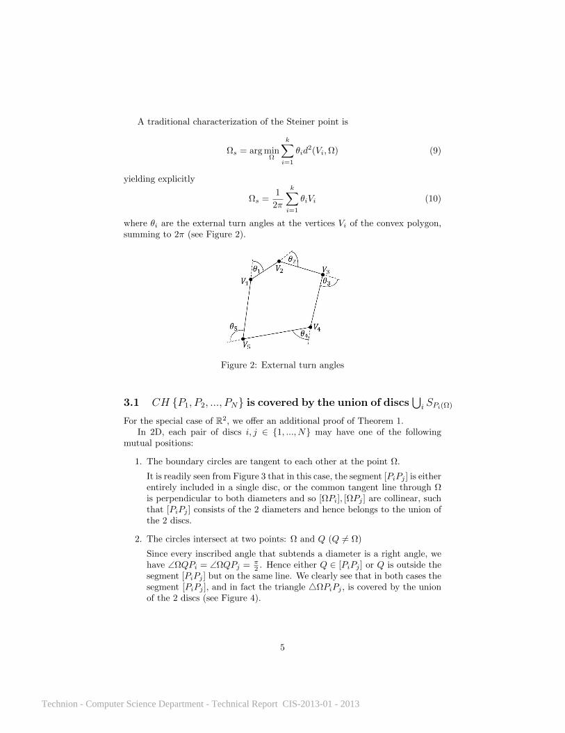
where θi are the external turn angles at the vertices Vi of the convex polygon,summing to 2π (see Figure 2).

Figure 2: External turn angles

3.1 CH P1, P2, ..., PN is covered by the union of discs⋃

i SPi(Ω)

For the special case of R2, we offer an additional proof of Theorem 1.In 2D, each pair of discs i, j ∈ 1, ..., N may have one of the following

mutual positions:

1. The boundary circles are tangent to each other at the point Ω.

It is readily seen from Figure 3 that in this case, the segment [PiPj ] is eitherentirely included in a single disc, or the common tangent line through Ωis perpendicular to both diameters and so [ΩPi], [ΩPj ] are collinear, suchthat [PiPj ] consists of the 2 diameters and hence belongs to the union ofthe 2 discs.

2. The circles intersect at two points: Ω and Q (Q 6= Ω)

Since every inscribed angle that subtends a diameter is a right angle, wehave ∠ΩQPi = ∠ΩQPj = π

2 . Hence either Q ∈ [PiPj ] or Q is outside thesegment [PiPj ] but on the same line. We clearly see that in both cases thesegment [PiPj ], and in fact the triangle 4ΩPiPj , is covered by the unionof the 2 discs (see Figure 4).

5


(a) (b)

Figure 3: Tangent circles (case 1)

(a) (b)

Figure 4: Intersecting circles (case 2)

So far it was shown that for every pair of discs i, j, the line segment [PiPj ],and in fact the triangle 4ΩPiPj , is covered by the union of the 2 discs.

The convex hull of a finite set of points in R2 is a convex polygon whosevertices are a subset of the point set P1, P2, ..., PN. Therefore the CH polygonedges are a subset of all possible segments [PiPj ] ∀i, j. As each such segment,and hence each polygon edge, belongs to the union of 2 discs, it obviously belongsto the union of all discs.

Since all the discs intersect at Ω, the union of discs is a star-shaped region,i.e.

∀Q0 ⊂N⋃i=1

SPi(Ω), [ΩQ0] ⊂

N⋃i=1

SPi(Ω) (11)

Due to this fact, together with the convexity of the CH polygon, the CH iscompletely covered by the union of triangles

⋃Ni,j=14ΩPiPj . Finally, since each

such triangle is covered by the union of discs, it follows that

∀Ω : CHP1, ..., PN ⊂N⋃i=1

SPi(Ω) (12)

6


3.2 The optimal location for Ω

Next, let us determine the optimal location of Ω in the sense of minimizing thearea difference between the union of discs SPi

(Ω), i = 1, 2, ..., N and the convexhull CH P1, P2, ..., PN. Clearly this requires us to simply minimize the area

of⋃Ni=1 SPi

(Ω).Denote by ∆S(Ω) the ”overflow” region covered beyond CH P1, P2, ..., PN,

i.e.

∆S(Ω) =

N⋃i=1

SPi(Ω) \ CH P1, P2, ..., PN (13)

We consider possible locations for Ω∗ only in the convex hull of the datapoints. Clearly, if Ω∗ would be outside CH P1, P2, ..., PN, we could add it tothe data points and get a set P1, P2, ..., PN ,Ω

∗ for which the optimal locationis a-priori known to be Ω∗, a point located on the boundary of the convexhull of the points P1, P2, ..., PN ,Ω

∗. However, we shall next show that for aconvex polygonal region, the optimal point is a (positively) weighted sum of theexternal points, hence it cannot be any one of them. From this it follows thatΩ∗ will have to be inside the convex hull of P1, P2, ..., PN. Therefore we shallprove the following:

Theorem 2. The area of ∆S(Ω) is minimized when Ω is located at the Steinercenter of the convex hull of the data points in R2.

Proof of Theorem 2.We consider Ω ⊂ CH P1, P2, ..., PN, which after reordering and renum-

bering the extremal points from P1, P2, ..., PN is a convex polygon defined byP1, P2, ..., PM

: (P1 → P2 → ...→ PM → P1).

It is readily seen that the N −M points in the interior of the convex hullpolygon define discs that are covered by the M discs determined by the externalpoints.

Indeed, if Pk is a point in P1, P2, ..., PN \P1, P2, ..., PM

we have that

SPk(Ω) ⊂ SPk

(Ω) where Pk is the point where the ray [ΩPk) exits the convexhull (see Figure 5)

The point Pk is on a boundary segment[PlPl+1

]of the convex hull and

SPl(Ω) ∪ SPl+1

(Ω) clearly covers SPk(Ω), since all three circles intersect at Ω

and at its projection on the line(PlPl+1

), denoted by Ql (see Figure 6).

Therefore let us define the shape S ,⋃Mi=1 SPi

(Ω) and compute its areaexplicitly as a function of the location of Ω.

Consider the convex polygon P1, P2, ..., PM → P1 and the point Ω inside it(see Figure 7).

7


Figure 5: Discs defined by internal points are covered by discs defined by exter-nal poins

Figure 6: The discs SPl(Ω),SPl+1

(Ω) and SPk(Ω) intersect at Ω and Ql

Figure 7: The convex polygon P1, P2, ..., PM → P1 with an internal point Ω

The diameters[ΩPi

]are segments that form a ”star configuration” about

Ω, their length being di , d[ΩPi

]. Let us denote by Qi the projections of Ω on

8


the lines(PiPi+1 (mod M)

). Also define the angles

∠PiΩQi = αi

∠QiΩPi+1 = βi+1

i = 1, 2, ...,M

as illustrated in Figure 8.

(a)

(b) (c)

Figure 8: Definition of the angles αi, βi+1 for the different possible locations ofQi

We recall the following simple facts about areas of segments in a circle (seeFigure 9):

Figure 9: Basic properties of triangles and circular segments

9


1. The area of a circular segment is given by

S(segment)(QP ) =1

4d2

(α− 1

2sin(2α)

)(14)

2. The area of the triangle ΩQP is

S(4ΩQP ) =1

4d2 sin(2α) (15)

Plugging (15) into (14), we can express

S(segment)(QP ) =1

4d2α− 1

2S(4ΩQP ) (16)

With these preliminary definitions and basic facts in mind, we can calculatethe area of the union of discs

⋃Mi=1 SPi

(Ω) and the area of the convex hullCH

P1, P2, ..., PM

in terms of the distances di and the angles αi and βi (see

Figure 10).

Figure 10: Computing the excess area ∆S and the area of the convex hull SCH(note that θk+1 = ∠QkΩQk+1 = ∠QkΩPk+1 + ∠Pk+1ΩQk+1 = βk+1 + αk+1)

Let us express the excess area ∆S defined in (13) as a sum of circular seg-ments. It can be seen from Figure 8 that the excess area over the CH edge[PiPi+1] in the three possible scenarios is either the sum or difference of thecircular segments lying on the chords [QiPi], [QiPi+1].

If Q ∈ [PiPi+1] (see Figure 8a), the excess area over [PiPi+1], denoted ∆Si,is

∆Si = S(segment)

(QiPi

)+ S(segment)

(QiPi+1

)and

S(4PiΩPi+1) = S(4PiΩQi) + S(4QiΩPi+1)

10


Thus using (16),

∆Si =

[1

4d2iαi −

1

2S(4PiΩQi)

]+

[1

4d2iβi+1 −

1

2S(4QiΩPi+1)

]=

1

4d2i (αi + βi+1)− 1

2

[S(4PiΩQi) + S(4QiΩPi+1)

]=

1

4d2i (αi + βi+1)− 1

2S(4PiΩPi+1)

(17)

Observing that ∠PiΩPi+1 = αi + βi+1, this yields

∆Si =1

4d2i

(∠PiΩPi+1

)− 1

2S(4PiΩPi+1) (18)

If Q 6∈ [PiPi+1] and is on the continuation of the line determined by [PiPi+1]beyond Pi+1 (see Figure 8b),

∆Si = S(segment)

(QiPi

)− S(segment)

(QiPi+1

)and

S(4PiΩPi+1) = S(4PiΩQi)− S(4QiΩPi+1)

with ∠PiΩPi+1 = αi − βi+1, resulting in

∆Si =

[1

4d2iαi −

1

2S(4PiΩQi)

]−[

1

4d2iβi+1 −

1

2S(4QiΩPi+1)

]=

1

4d2i (αi − βi+1)− 1

2

[S(4PiΩQi)− S(4QiΩPi+1)

]=

1

4d2i

(∠PiΩPi+1

)− 1

2S(4PiΩPi+1)

(19)

Finally, if Qi is on the line determined by [Pi+1Pi] beyond Pi (see Figure 8c),

∆Si = −S(segment)

(QiPi

)+ S(segment)

(QiPi+1

)and

S(4PiΩPi+1) = −S(4PiΩQi) + S(4QiΩPi+1)

with ∠PiΩPi+1 = −αi + βi+1, we similarly get

∆Si =1

4d2i (−αi + βi+1)− 1

2

[−S(4PiΩQi) + S(4QiΩPi+1)

]=

1

4d2i

(∠PiΩPi+1

)− 1

2S(4PiΩPi+1)

(20)

Therefore, summing the excess area over all the M discs, we can write:

∆S =

M∑i=1

∆Si =

M∑i=1

d2i

4

(∠PiΩPi+1

)− 1

2S(4PiΩPi+1) (21)

11


Observe that the convex hull area can similarly be expressed as a sum oftriangles:

SCH =

M∑i=1

S(4PiΩPi+1) (22)

Given that observation, we can rewrite (21) as:

∆S =

M∑i=1

d2i

4

(∠PiΩPi+1

)− 1

2SCH (23)

Now we wish to find the optimal center that yields the minimal excess area,and since SCH is independent of Ω, we need to solve:

Ω∗ = arg minΩ

∆S = arg minΩ

M∑i=1

d2i

(∠PiΩPi+1

)(24)

By extending each edge [Pi−1Pi] outside the polygon, an exterior angle isformed at the vertex Pi whose size is exactly θi = ∠PiΩPi+1 (see Figure 10).As θi is also independent of Ω, (24) becomes:

Ω∗ = arg minΩ

M∑i=1

θid2i (25)

This is simply a weighted sum of the square distances of the vertices fromΩ, with given constant weights that measure the exterior angles of the convexpolygon. Noting that the M exterior angles sum to 2π, the optimizer of (25) isexplicitly given by:

Ω∗(x, y) =

(M∑i=1

θi2πxi,

M∑i=1

θi2πyi

)(26)

We see that a relatively straightforward calculation provides the optimallocation Ω∗ as a weighted average of the points P1, P2, ..., PM , the weights beingproportional to the turn angles at Pi.

However this is exactly the Steiner center point of the convex polygon de-fined by the points P1, P2, ..., PN .

Hence Theorem 2 is proved, and also, we have justified the search for theoptimal location only within the convex hull of the data points.

4 The Steiner center: some alternative charac-terizations

The Steiner point (also known as the Steiner curvature centroid) of a convexpolygon in R2, is commonly defined as the geometric centroid of the system

12


obtained by placing a mass equal to the magnitude of the exterior angle at eachvertex [4].

For a set of points P ⊆ R2, let VP be the set of extreme points of P , i.e. thevertices of the convex hull CH(P ). For every p ∈ VP let αp be the interior angleformed on the convex hull boundary at p, and set the weights accordingly:

w(p) =

π − αp, if p ∈ VP0 if p ∈ P − VP

(27)

such that for p ∈ VP the weight w(p) is the turn angle at p on CH(P ).The Steiner point is defined as the normalized weighted center of mass of P

using the weights w(p). Since∑p∈P w(p) = 2π, this center is:

Ωs(P ) =1

2π

∑p∈P

w(p)p (28)

An interesting property of the Steiner point arising from this definition isthat it is defined solely by the geometry of the convex hull, i.e. given a discreteset of points P , their Steiner center takes into consideration only the subset ofthese points that serve as vertices of CH(P ). A desirable consequence is the”stability” of this center, in the sense that a continuous displacement of anypoint p ∈ P results in a continuous change of the weights and therefore also ofthe Steiner center [3].

Another characterization of the Steiner center is by projections [3]: Denotethe unit vector at angle θ ∈ [0, π) by uθ = (cosθ, sinθ). Let Pθ denote theprojection of the set of points P ⊆ R2 on uθ, then:

Pθ = uθ < p, uθ > | p ∈ P (29)

and the Steiner center is defined as:

Ωs(P ) =2

π

∫ π

0

mid(Pθ)dθ (30)

where:mid(Pθ) =

uθ2

( minp∈P

< p, uθ >+ maxp∈P

< p, uθ >) (31)

is simply the Euclidean center of Pθ.

Additionally, the Steiner center Ωs of a convex shape has some very interest-ing properties, among which is its linearity with respect to Minkowski addition.That is, if K1 and K2 are two convex sets in Rd, we have that

Ωs(K1 ⊕K2) = Ωs(K1) + Ωs(K2) (32)

where ⊕ stands for vector addition, i.e.

K1 ⊕K2 = x+ y|x ∈ K1, y ∈ K2 (33)

13


It is also true that the map K → Ωs(K) is similarity invariant, i.e.

Ωs(tK) = tΩs(K) (34)

wheretK =

tx|x ∈ K ⊂ Rd, t > 0

(35)

It is well known (see Shephard [11, 13], Sallee [8] and Schneider [9]) that theabove two properties and continuity of a mapping characterize the Steiner point,i.e. if we have a mapping from the set of convex shapes to Rd, i.e. Φ : Pd → Rd(where Pd is the set of convex shapes in Rd) that satisfies:

1. Φ(K1 ⊕K2) = Φ(K1) + Φ(K2)

2. Φ(tK) = tΦ(K)

3. Φ() is continuous

then necessarily Φ(K) = Ωs(K).

We hope that this last characterization will enable an elegant proof of theresult discussed in this paper for the higher dimensional case.

5 Concluding remarks

This paper presented a novel characterization of the Steiner center as the pointthat provides the tightest disc coverage for the convex hull of the set of pointsin the plane.

We first proved that the convex hull of N points in Rd is covered by theunion of d-dimensional discs formed such that their diameters are the segmentsconnecting some point Ω inside the convex hull with each of the N vertices (thisis true for any Ω chosen inside the convex hull, regardless of its exact location).

Next it was shown for R2 that the theoretically optimal location of Ω inthe sense of minimizing the area difference between the union of discs and theconvex hull is the well known Steiner curvature center. This interesting propertyis a nice addition to the existing characterizations of the Steiner center.

For higher dimensions, we conjecture that the optimal point is the Rd Steinercenter, but a theoretical proof is yet to be found. Some numerical simulationsthat were performed in 3D seem to confirm this conjecture.

Acknowledgements

This research was supported by the Israel Science Foundation grant no. 1551/09.

14


References

[1] C. Berg. Abstract Steiner points for convex polytopes. J. London Math.Soc., 4(1):176–180, 1971.

[2] P. Carmi, S. Har-Peled, and M. J. Katz. On the Fermat-Weber center ofa convex object. Comput. Geom. Theory Appl., 32:188–195, 2005.

[3] S. Durocher and D. Kirkpatrick. The Steiner center of a set of points:stability, eccentricity, and applications to mobile facility location. Interna-tional Journal of Computational Geometry & Applications, 16(4):345–371,2006.

[4] R. Honsberger. Episodes in Nineteenth and Twentieth Century EuclideanGeometry. The Mathematical Association of America, 1995.

[5] M. J. Kaiser and T. L. Morin. Characterizing centers of convex bodies viaoptimization. J. Math. Anal. and Applications, 184(3):533–559, 1994.

[6] D. Keren, I. Sharfman, A. Schuster, and A. Livne. Shape sensitive geomet-ric monitoring. IEEE Trans. Knowl. Data Eng., 24(8):1520–1535, 2012.

[7] P. McMullen. Valuations and Euler-type relations on certain classes ofconvex polytopes. Proc. London Math. Soc., 35:113–135, 1977.

[8] G. T. Sallee. A valuation property of Steiner points. Mathematika, 13:76–82, 1966.

[9] R. Schneider. On Steiner points of convex bodies. Israel J. Math., 9(2):241–249, 1971.

[10] I. Sharfman, A. Schuster, and D. Keren. A geometric approach to mon-itoring threshold functions over distributed data streams. In Proc. ACMSIGMOD Int’l Conf. Management of Data (SIGMOD ’06), pages 301–312,2006.

[11] G. C. Shephard. The Steiner point of a convex polytope. Canad. J. Math,18:1294–1300, 1966.

[12] G. C. Shephard. Euler-type relations for convex polytopes. Proc. LondonMath. Soc., 18(4):597–606, 1968.

[13] G. C. Shephard. A uniqueness theorem for the Steiner point of a convexregion. J. London Math. Soc., 43:439–444, 1968.

15


on optimal disc covers and a new characterization of the ... · i=1 s p i (), arose in the analysis...

Documents