On Strong Stability of Explicit Runge–KuttaMethods for Nonlinear Semibounded Operators

Hendrik Ranocha

21 May 2019

Explicit Runge–Kutta methods are classical and widespread techniques in thenumerical solution of ordinary differential equations (ODEs). Considering partialdifferential equations, spatial semidiscretisations can be used to obtain systems ofODEs that are solved subsequently, resulting in fully discrete schemes. However,certain stability investigations of high-order methods for hyperbolic conservationlaws are often conducted only for the semidiscrete versions. Here, strong stability(also known as monotonicity) of explicit Runge–Kutta methods for ODEs withnonlinear and semibounded (also known as dissipative) operators is investigated.Contrary to the linear case, it is proven that many strong stability preserving (SSP)schemes of order two or greater are not strongly stable for general smooth andsemibounded nonlinear operators. Additionally, it is shown that there are first orderaccurate explicit SSP Runge–Kutta methods that are strongly stable (monotone) forsemibounded (dissipative) and Lipschitz continuous operators.

Keywords. Runge–Kutta methods · strong stability ·monotonicity · strong stabilitypreserving · semibounded ·dissipativeMathematics Subject Classification (2010). 65L06 · 65L20 · 65M12 · 65M20

1 Introduction

Considering the numerical solution of (partial) differential equations, stability of the schemesplays an important role. For linear symmetric hyperbolic partial differential equations (PDEs),energy estimates can often be obtained, resulting in both uniqueness of solutions and existencevia appropriate approximations, as described in the monographs of Gustafsson, Kreiss andOliger [18] and Kreiss and Lorenz [30]. Using schemes in the framework of summation byparts operators [31] with simultaneous approximation terms [8, 9], these energy estimates canoften be transferred to semidiscrete schemes, as described in the review articles of Fernández,Hicken and Zingg [14] and Svärd and Nordström [49] and references cited therein. While thisframework has been developed originally for finite difference schemes, it contains also manyother classes of methods such as finite volume [35, 36], discontinuous Galerkin [13, 16], andflux reconstruction schemes [26, 43].Since numerical methods are used to obtain fully discrete schemes from semidiscrete ones,

the preservation of such kind of semidiscrete stability is worth investigating. Strong stabilitypreserving (SSP)methods can bewritten as convex combinations of explicit Euler steps. Hence,they preserve all convex stability properties of the explicit Euler method, as described in themonograph of S. Gottlieb, Ketcheson and Shu [17] and references cited therein.However, even for linear ODEs with semibounded operators, the explicit Euler method does

not preserve L2 stability in general. Thus, the SSP property cannot be used to obtain strongstability for these schemes. Nevertheless, some well-known high order, explicit SSP Runge–Kutta methods are strongly stable in this general case [42, 51]. While the classical fourth orderRunge–Kutta method is not strongly stable after one time step, combining two consecutive time

1

arX

iv:1

811.

1160

1v2

[m

ath.

NA

] 1

5 D

ec 2

019

steps results in a strongly stable scheme for this class of problems [47]. Further results for linearautonomous systems have been obtained by Sun and Shu [48].

Becausemany hyperbolic conservation laws are nonlinear or semidiscretisations are obtainedvia nonlinear processes, it is interesting whether explicit SSP Runge–Kutta methods can bestrongly stable for general nonlinear ODEs with semibounded operators. In the context ofhyperbolic conservation laws, many studies are based on the seminal work of Tadmor [50, 52]concerning entropy stability of semidiscretisations. While there are related studies of explicitRunge–Kutta methods [33], there are no general results on strong stability.

Although strong stability can be considered for general convex functionals, the L2 norm willbe used in this article. It is most similar to the linear case and of interest in applications,e.g. in the recent article of Nordström and La Cognata [37]. Moreover, it is a special case ofstrong stability and it might be expected that there is a larger set of methods that are stronglystable for this convex functional, similar to the case of SSP methods studied by Higueras [22].Furthermore, the focus is on explicit schemes, since they are widespread, can be implementedeasily, are oftenmore efficient if accuracy is a determining factor, and efficient use of parallelismis less expensive than for implicit schemes [28].

In this article, it is proven that many explicit SSP Runge–Kutta methods of order two orgreater cannot be strongly stable for nonlinear ODEs with smooth and semibounded operatorsin general. Some tedious calculations used in these proofs are verified using Mathematica [53]and published online [41]. Moreover, it is shown that first order accurate schemes can be bothSSP and strongly stable for semibounded and Lipschitz continuous operators.

To do so, the article is structured as follows. At first, basic definitions such as strong stabilityand semiboundedness are given in section 2. Additionally, a brief review of Runge–Kuttamethods is included to introduce the notation. Afterwards, Runge–Kutta methods of up tothree stages are studied in section 3. It is shown that there are no such schemes with orderof accuracy of at least two that are strongly stable and SSP. This result is based on the explicitconstruction of ODEswith nonlinear and semibounded operators and implications of the orderconditions.

Since the number of parameters and the complexity of the order conditions increases withthe number of stages, the general approach is not really feasible for methods with more stages.Therefore, some known explicit SSP methods with more than three stages are investigatedseparately in section 4. In particular, it is shown that the families of schemes with optimal SSPcoefficient of order two [29, Theorem 9.3] and three [27, Theorem 3] and the ten stage, fourthorder method SSPRK(10,4) of Ketcheson [27] are not strongly stable in general.

Thereafter, two well-known and popular SSP methods are studied in more detail in thefollowing sections. While the investigations up to this point are only concerned with strongstability and not with boundedness in general, the popular three-stage method SSPRK(3,3) ofShu and Osher [45] is studied in detail in section 5. It is shown that the norm of the numericalapproximation can increasemonotonically andwithout bounds for nonlinear and semiboundedoperators. Since this article is motivated by applications of SSP methods to semidiscretisationsof hyperbolic conservation laws, an energy stable and nonlinear semidiscretisation of the lineartransport equation is constructed in section 6. This ODE with semibounded operator is solvednumerically with SSPRK(10,4) and it is shown that the norm of the numerical solution increasesfor a large range of time steps.

Turning to first order schemes in section 7, it is shown that the limitations of high orderschemes studied before do not apply. In particular, there are explicit SSP Runge–Kuttamethodsof first order of accuracy that are strongly stable for semibounded and Lipschitz continuousoperatorswithLipschitz constant L under a time step restriction∆t ≤ ∆tmax, where∆tmax ∝ L−1.Finally, the results are summarised and discussed in section 8.

2

2 Brief Review of Runge Kutta Methods

Consider an ordinary differential equation

ddt u(t) � g

(u(t)) , t ∈ (0, T),

u(0) � u0 ,(2.1)

in a real vector space H with semi inner product 〈·, ·〉, inducing the seminorm ‖·‖. Typically,H can be a Hilbert space. Therefore, ‖·‖ will be called norm in the following. However, theproperty distinguishing a norm from a seminorm will not be used anywhere.

2.1 Strong Stability

For a smooth solution of (2.1), the time derivative of the squared norm is

ddt

u(t) 2� 2

⟨u(t), d

dt u(t)⟩� 2

⟨u(t), g

(u(t))⟩ . (2.2)

Definition 2.1. A function g : H →H is semibounded, if

∀u ∈ H :⟨u , g(u)⟩ ≤ 0. (2.3)

/

Remark 2.1. If a complex (semi) inner product space is considered instead of a real one, the realpart of the (semi) inner product

⟨u , g(u)⟩ has to be non-positive. /

Remark 2.2. Sometimes, such operators g are also called (energy) dissipative. Here, the termsemibounded is used instead, in order to emphasise that (energy) conservative operators areincluded in this definition. /

Thus, the (squared) norm of a smooth solution u of (2.1) is bounded by its initial value if gis semibounded. However, an approximate solution obtained by a numerical method does notnecessarily satisfy this inequality. For example, applying one step of the explicit Euler methodto (2.1) yields the new value u+ � u0 + ∆t g(u0), satisfying

‖u+‖2 � u0 + ∆t g(u0)

2� ‖u0‖2 + 2∆t

⟨u0 , g(u0)

⟩︸¨ ¨ ¨ ¨ ¨ ¨ ¨︷︷¨ ¨ ¨ ¨ ¨ ¨ ¨︸

≤0

+∆t2 g(u0) 2

︸¨ ¨ ¨ ¨ ¨︷︷¨ ¨ ¨ ¨ ¨︸≥0

. (2.4)

Thus, for a general semibounded g, the norm of the numerical solution can increase duringone time step, e.g. if

⟨u0 , g(u0)

⟩� 0. In particular, this happens if g(u) � Lu where L is a

linear and skew-symmetric operator.Definition 2.2. A numerical scheme approximating (2.1) during one time step from u0 ≈ u(t)to u+ ≈ u(t + ∆t)with semibounded g is called strongly stable if ‖u+‖2 ≤ ‖u0‖2. /

Remark 2.3. Since this work is motivated by discretisations of PDEs, the term strong stability isused. In the literature on Runge–Kuttamethods, such a property is often calledmonotonicity. /

Nevertheless, the explicit Euler method can be strongly stable under stronger assumptionson g. For example, consider the condition

∃M ∈ R∀u ∈ H :⟨u , g(u)⟩ ≤ M

g(u) 2. (2.5)

If M < 0 in (2.5), the explicit Euler method u+ � u0 + ∆t g(u0) is strongly stable under the timestep restriction ∆t ∈ (0,−2M], since

u0 + ∆t g(u0) 2 −‖u0‖2 � 2∆t

⟨u0 , g(u0)

⟩+ ∆t2 g(u0)

2 ≤ (∆t + 2M)∆t g(u0)

2 ≤ 0. (2.6)

Such right hand sides with linear g are called coercive by Levy and Tadmor [32] and Tadmor[51].

3

Remark 2.4. Instead of the norm‖·‖ of the solution, other convex functionals can be considered.For semidiscretisations of hyperbolic conservation laws, some important examples are the L1

norm u(t) 1 �

∫ ��u(t , x)�� dx, the total variation seminorm u(t) TV , non-negativity (expressed

via −minx u(t , x)), or the total entropy∫

U(u(t , x)) dx, where U is a convex function. In that

case, strong stability refers to the monotonicity of that particular convex functional in time. /

Since the explicit Euler method is relatively simple, it is desirable to transfer results such asstrong stability from that method (which are relatively easy to check) to high order schemes (forwhich it is considerably more difficult to check these properties). Strong stability preservingnumerical schemes are designed to enable exactly this transfer, as described in the monographof S. Gottlieb, Ketcheson and Shu [17] and references cited therein.Definition 2.3. A numerical time scheme for (2.1) is called strong stability preserving (SSP) withSSP coefficient c > 0 if it is strongly stable under the time step restriction ∆t ≤ c∆tE wheneverthe explicit Euler method is strongly stable for ∆t ≤ ∆tE and any convex functional, i.e. if for allconvex functionals η, ∀∆t ∈ (0,∆tE] : η(u0 +∆t g(u0)) ≤ η(u0) implies ∀∆t ∈ (0, c∆tE] : η(u+) ≤η(u0). /

Considering only semi inner products as in this article, some restrictions for general SSPmethods can be relaxed [22].

2.2 Connections to Other Properties

The application of a one-sided Lipschitz condition

∃M ∈ R∀t ∈ [0, T], u , v ∈ X :⟨

f (t , u) − f (t , v), u − v⟩ ≤ M‖u − v‖2 (2.7)

has been very successful, e.g. for stiff and dissipative problems

ddt u(t) � f

(t , u(t)) , t ∈ (0, T),

u(0) � u0 ,(2.8)

cf. Söderlind [46]. Indeed, the existence of such a one-sided/logarithmic Lipschitz con-stant M implies that the difference between two solutions u , v of (2.8) with initial conditionsu0 , v0 remains bounded. In particular, if M ≤ 0, the difference between two solutions doesnot increase, resulting in contractivity. Thus, such a condition yields some important stabil-ity/boundedness/robustness properties. Since (2.7) does not restrict the Lipschitz seminorm

�� f��Lip :� sup

u,v

f (t , u) − f (t , v) ‖u − v‖ (2.9)

of f , results based thereon can be applied to arbitrarily stiff equations. Hence, it is mostlyuseful for implicit methods. In order to be able to investigate also stability properties of explicitmethods, Dahlquist and Jeltsch [11] introduced the condition

∃M ∈ R∀t ∈ [0, T], u , v ∈ X :⟨

f (t , u) − f (t , v), u − v⟩ ≤ M

f (t , u) − f (t , v) 2, (2.10)

see also Dekker and Verwer [12, Chapter 6]. If f satisfies (2.10) with M < 0, f is Lipschitzcontinuous in its second argument with

�� f��Lip ≤ −M−1, since

−M f (t , u) − f (t , v) 2 ≤ − ⟨

f (t , u) − f (t , v), u − v⟩ ≤ f (t , u) − f (t , v) ‖u − v‖ . (2.11)

M < 0 yields again a contractive ODE and results based on (2.10) can be applied to explicitmethods since the Lipschitz constant of f is bounded.

General results on contractivity can be implied by seemingly simpler requirements such as

∃M ∈ R∀t ∈ [0, T], u ∈ X :⟨

f (t , u), u⟩≤ M‖u‖2 (2.12)

or∃M ∈ R∀t ∈ [0, T], u ∈ X :

⟨f (t , u), u

⟩≤ M

f (t , u) 2, (2.13)

4

cf. [6] or [7, Section 357]. In particular, monotonicity/semiboundedness results such as discreteversions of

u(t) ≤ ‖u0‖ can be transferred directly to contractivity. Therefore, only the formerwill be studied in this article.Remark 2.5. For linear ODEs with possibly time dependent coefficients, the concepts of con-tractivity and monotonicity are equivalent. Since many results have been established for con-tractivity, e.g. byDahlquist and Jeltsch [11] andDekker andVerwer [12], they can be transferreddirectly to monotonicity. In particular, severe limitations of numerical methods result from lin-ear ODEs with varying coefficients. /

Remark 2.6. Results for right hand sides f satisfying (2.13) with M < 0 have been obtainedby Higueras [22], similar to the results for circle contractivity by Dahlquist and Jeltsch [11]and Dekker and Verwer [12]. This is a special case of strong stability preservation and ismore directly related to semibounded operators considered in this article. Nevertheless, sincenumerical methods for hyperbolic conservation laws motivate this study, general SSP methodswill be considered. /

Remark 2.7. For linear and time-independent ODEs (2.1) with semibounded g, some strongstability properties have been obtained by Ranocha andÖffner [42] and Sun and Shu [48]. Thus,it is interesting whether similar results can be established under the assumption (2.13) withM ≤ 0. In order to restrict the stiffness of the ODE (2.1), a Lipschitz condition will be assumed,i.e.

��g��Lip ≤ L. Since there are many negative results even for autonomous problems, (2.1) willbe considered instead of (2.8). /

2.3 Runge–Kutta Methods

A general (explicit or implicit) Runge–Kutta method with s stages can be described by itsButcher tableau [7, 20]

c Ab (2.14)

whereA ∈ Rs×s and b , c ∈ Rs . Since (2.1) is an autonomousODE, there is no explicit dependencyon time and one step from u0 to u+ is given by

ui � u0 + ∆ts∑

j�1ai j g(u j), u+ � u0 + ∆t

s∑i�1

bi g(ui). (2.15)

Here, ui are the stage values of the Runge–Kutta method. It is also possible to express themethod via the slopes ki � g(ui) [19, Definition II.1.1].

Using the stage values ui as in (2.15), the change of squared norm (“energy”) is given by

‖u+‖2 −‖u0‖2 � 2∆t

⟨u0 ,

s∑i�1

bi g(ui)⟩+ (∆t)2

s∑

i�1bi g(ui)

2

(2.16)

(2.15)� 2∆t

s∑i�1

bi

⟨ui − ∆t

s∑j�1

ai j g(u j), g(ui)⟩+ (∆t)2

s∑

i�1bi g(ui)

2

� 2∆ts∑

i�1bi

⟨ui , g(ui)

⟩+ (∆t)2

s∑

i�1bi g(ui)

2

− 2s∑

i , j�1bi ai j

⟨g(ui), g(u j)

⟩� 2∆t

s∑i�1

bi⟨ui , g(ui)

⟩+ (∆t)2

s∑

i , j�1

(bi b j − bi ai j − b j a ji

) ⟨g(ui), g(u j)

⟩,

where the symmetry of the scalar product has been used in the last step. Here, the first termon the right hand side is consistent with

∫ t0+∆tt0

2⟨u(t), g

(u(t))⟩ dt, if the Runge–Kutta method

5

is consistent, i.e.∑s

i�1 bi � 1. Additionally, it can be estimated via the semiboundedness of g ifall bi are non-negative.

The second term of order (∆t)2 is undesired. Depending on the method (and the stages, ofcourse), it may be positive or negative. However, if it is positive, then a stability error may beintroduced.

As a special case, if the method fulfils bi b j � bi ai j + b j a ji , i , j ∈ {1, . . . , s}, this term vanishes.These methods can conserve quadratic invariants of ordinary differential equations, a topicof geometric numerical integration, see Theorem IV.2.2 of Hairer, Lubich and Wanner [19],originally proved by Cooper [10]. A special kind of these methods are the implicit Gaußmethods [19, Section II.1.3].More generally, the (∆t)2 term is non-positive if thematrixwith entries (bi b j−bi ai j−b j a ji)i , j is

negative semidefinite (and bi ≥ 0, as before), i.e. when the Runge–Kutta method is algebraicallystable. Then, the Runge–Kutta method is strongly stable in the L2 norm for every time step∆t > 0, i.e. B stable, cf. [7, section 357]. While there are Runge–Kutta methods with these nicestability properties, these are all implicit.Remark 2.8. Applying explicit methods to (2.1), it can be expected that time step restrictionsfor strong stability depend on boundedness or Lipschitz constants of g, e.g. ∆t ≤ ∆tmax ∝ L−1.Hence, such restrictions on g will be used in the following. /

The following result will be used in the next sections, cf. [17, Observation 5.2] or [29].Lemma 2.1. Any Runge–Kutta method with positive SSP coefficient c > 0 has non-negative coefficientsand weights, i.e. ∀i , j : ai j ≥ 0, bi ≥ 0.

That the coefficients ai j , bi of the schemes are non-negative can also be obtained under otherconditions focusing on circle contractivity, cf. [22]. This implies certain restrictions on thepossible order of the schemes, cf. [29] or [17, Section 5.1].

3 Explicit Methods with Three Stages

In this section, explicit Runge–Kutta methods with three stages are considered. Thus, thecorresponding coefficients are

a21 , a31 , a32 , b1 , b2 , b3. (3.1)

Since the proofs of the negative results obtained in this section are easier if fewer coefficientsare considered, third order methods will be investigated at first. Thereafter, schemes of at leastsecond order of accuracy are studied.The usual conditions for second order accurate Runge–Kuttamethods used later are

∑sj�1 b j �

1 and∑s

j,k�1 b j a jk � 1/2. Thirdorder schemeshave to fulfil∑s

j,k ,l�1 b j a jk a jl � 1/3and∑sj,k ,l�1 b j a jk akl �

1/6 additionally [20, Section II.2].The basic approach to get negative results can be described as follows. Certain test problems

(2.1) using specific semibounded g are constructed such that the normof the numerical solutionincreases during the first time step for each ∆t ∈ (0,∆tmax]. Then, this result can be transferredto semibounded g with

��g��Lip ≤ L by considering suitable modifications outside of a boundedregion using Kirszbraun’s theorem [44, Theorem 1.31]:Theorem 3.1 (Kirszbraun). Suppose S is a subset of the Hilbert spaceH and g : S → H is Lipschitzcontinuous. Then, g can be extended to all of H in such a way that the extension satisfies the sameLipschitz condition.

3.1 Third Order Methods

Theorem 3.2. There is no explicit Runge–Kutta method that

• is strong stability preserving with positive SSP coefficient,

• is of third order of accuracy & has at most three stages,

6

• and is strongly stable for (2.1) for all smooth and semibounded g with��g��Lip ≤ L.

To prove Theorem 3.2, the initial value problem (2.1) with

u(t) �(u1(t)u2(t)

), g(u) � α(u1 − ru2)

(−u2u1

), u0 �

(10

), (3.2)

will be used, where r is a real parameter, α > 0, and u1 , u2 are real valued functions. Since g isgiven by polynomials in u, the squared norm after one step can be calculated explicitly and isa polynomial in the time step ∆t.Lemma 3.1. Applying an explicit third order Runge–Kutta method with three stages given by theparameters (3.1) to the ODE (2.1) with (3.2) yields ‖u+‖2 − ‖u0‖2 � ∆t4p(∆t), where p(∆t) is apolynomial of the form

p(∆t) � α4

12

(−5 + 7r2

+ (a31 + a32)(4 − 8r2))+ O(∆t). (3.3)

Lemma 3.1 can be proved by direct but tedious calculations and has been verified usingMathematica [53].Lemma 3.2. An explicit third order Runge–Kutta method with three stages given by the parameters (3.1)that is strongly stable for (2.1) for all smooth and semibounded g with

��g��Lip ≤ L satisfies

78 ≤ a31 + a32 ≤ 5

4 . (3.4)

Proof. In order to be strongly stable for the ODE (2.1) with (3.2), the coefficient of the constantterm of the polynomial p(∆t) given in Lemma 3.1 has to be non-positive, i.e.

12α4 p(0) � −5 + 7r2

+ (a31 + a32)(4 − 8r2) ≤ 0.

This can be reformulated as

a31 + a32 ≤ 5 − 7r2

4 − 8r2 , if r2 <12

a31 + a32 ≥ 5 − 7r2

4 − 8r2 , if r2 >12 .

(3.5)

Basically, the assertion is proved by letting r → 0 in the first inequality and r → ∞ in thesecond one. To satisfy the upper bound on the Lipschitz constant, α→ 0 can be coupled withthe limiting process on r: In this way, the local Lipschitz constant of g (3.2) around u0 can bemade arbitrarily small without changing the results of Lemma 3.2. Since only one time stepis considered, g can be modified outside of a suitable neighbourhood of u0 while keeping thelocal Lipschitz constant of g as global Lipschitz constant because of Kirszbraun’s theorem. �

These technical results can be used to prove Theorem 3.2 as follows.

Proof of Theorem 3.2. The general solution of the order conditions for third order explicit Runge–Kutta methods with three stages is given by the two parameter family

a21 � α2 , b1 � 1 +2 − 3(α2 + α3)

6α2α3,

a31 �3α2α3(1 − α2) − α2

3α2(2 − 3α2) , b2 �

3α3 − 26α2(α3 − α2) ,

a32 �α3(α3 − α2)α2(2 − 3α2) , b3 �

2 − 3α26α3(α3 − α2) ,

(3.6)

7

where α2 , α3 , 0, α2 , α3, α2 , 2/3 and the two one parameter families

a21 �23 , b1 �

14 ,

a31 �23 −

14ω3

, b2 �34 − ω3 ,

a32 �1

4ω3, b3 � ω3 ,

(3.7)

where α2 � α3 � 2/3 anda21 �

23 , b1 �

14 − ω3 ,

a31 �1

4ω3, b2 �

34 ,

a32 � − 14ω3

, b3 � ω3 ,

(3.8)

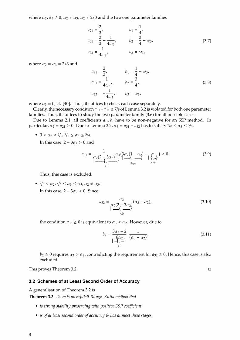
where α3 � 0, cf. [40]. Thus, it suffices to check each case separately.Clearly, the necessary condition a31+a32 ≥ 7/8 of Lemma 3.2 is violated for both one parameter

families. Thus, it suffices to study the two parameter family (3.6) for all possible cases.Due to Lemma 2.1, all coefficients ai j , bi have to be non-negative for an SSP method. In

particular, α2 � a21 ≥ 0. Due to Lemma 3.2, α3 � a31 + a32 has to satisfy 7/8 ≤ α3 ≤ 5/4.• 0 < α2 < 2/3, 7/8 ≤ α3 ≤ 5/4.

In this case, 2 − 3α2 > 0 and

a31 �1

α2(2 − 3α2)α3︸¨ ¨ ¨ ¨ ¨ ¨︷︷¨ ¨ ¨ ¨ ¨ ¨︸>0

(3α2(1 − α2)︸¨ ¨ ¨ ¨︷︷¨ ¨ ¨ ¨︸

≤3/4

− α3︸︷︷︸≥7/8

)< 0. (3.9)

Thus, this case is excluded.

• 2/3 < α2, 7/8 ≤ α3 ≤ 5/4, α2 , α3.In this case, 2 − 3α2 < 0. Since

a32 �α3

α2(2 − 3α2)︸¨ ¨ ¨ ¨︷︷¨ ¨ ¨ ¨︸<0

(α3 − α2), (3.10)

the condition a32 ≥ 0 is equivalent to α3 < α2. However, due to

b2 �3α3 − 2

6α2︸¨ ¨︷︷¨ ¨︸>0

1(α3 − α2) , (3.11)

b2 ≥ 0 requires α3 > α2, contradicting the requirement for a32 ≥ 0, Hence, this case is alsoexcluded.

This proves Theorem 3.2. �

3.2 Schemes of at Least Second Order of Accuracy

A generalisation of Theorem 3.2 isTheorem 3.3. There is no explicit Runge–Kutta method that

• is strong stability preserving with positive SSP coefficient,

• is of at least second order of accuracy & has at most three stages,

8

• and is strongly stable for (2.1) for all smooth and semibounded g with��g��Lip ≤ L.

The basic idea of the proof of Theorem 3.3 is the same as for the proof of Theorem 3.2.However, the technical details are a bit more complicated.

As before, the initial value problem (2.1) with (3.2) will be used, where r is a real parameter,α > 0, and u1 , u2 are real valued functions.Lemma 3.3. Applying an explicit three stage Runge–Kutta method with at least second order of accuracygiven by the parameters (3.1) to the ODE (2.1)with (3.2) yields‖u+‖2−‖u0‖2 � ∆t3p(∆t), where p(∆t)is a polynomial of the form

p(∆t) �(−1 + a21 − 2a21a31b3 + 2a2

31b3 + 4a31a32b3 + 2a232b3

)rα3

+14

(1 + r2 − 8a21a32b3(2 − r2

+ a31(−1 + 2r2) + a32(−1 + 2r2)))∆tα4

+ O(∆t2). (3.12)

Since the restrictions imposed by (3.2) do not seem to suffice to prove Theorem 3.3, the initialvalue problem (2.1) with

u(t) �(u1(t)u2(t)

), g(u) � α(ru1 − u2)

(−u2u1

), u0 �

(10

), (3.13)

will be used additionally, where r is again a real parameter and α > 0.Lemma 3.4. Applying an explicit three stage Runge–Kutta method with at least second order of accuracygiven by the parameters (3.1) to the ODE (2.1) with (3.13) yields ‖u+‖2 −‖u0‖2 � ∆t3p(∆t), wherep(∆t) is a polynomial of the form

p(∆t) �(−1 + a21 − 2a21a31b3 + 2a2

31b3 + 4a31a32b3 + 2a232b3

)r2α3

+14 r2

(1 + r2

+ 8a21a32b3(1 − 2r2

+ (a31 + a32)(−2 + r2)) ) ∆tα4+ O(∆t2). (3.14)

Both Lemma 3.3 and Lemma 3.4 can be proved by direct but tedious calculations and havebeen verified using Mathematica [53].

These technical results can be used to prove Theorem 3.3 as follows.

Proof of Theorem 3.3. For s � 3 stages, the conditions for an order of accuracy 2 are

s∑j�1

b j � 1,s∑

j,k�1b j a jk �

12 . (3.15a)

As in Lemma 3.2, the coefficient of the constant term of the polynomial p(∆t) in Lemma 3.3 hasto be non-positive for all r ∈ R. Since p(0) � (−1+a21−2a21a31b3+2a2

31b3+4a31a32b3+2a232b3)rα3,

this implies−1 + a21 − 2a21a31b3 + 2a2

31b3 + 4a31a32b3 + 2a232b3 � 0. (3.15b)

Furthermore, Lemma 3.3 (i.e. the right hand side (3.2)) yields the condition

∀r ∈ R : 1 + r2 − 8a21a32b3(2 − r2

+ (a31 + a32)(−1 + 2r2)) ≤ 0. (3.15c)

Similarly, Lemma 3.4 (i.e. the right hand side (3.13)) yields the condition

∀r ∈ R : r2(1 + r2

+ 8a21a32b3(1 − 2r2

+ (a31 + a32)(−2 + r2)) ) ≤ 0. (3.15d)

As in the proof of Lemma 3.2, α > 0 can be adapted to r such that the local Lipschitz constantof g near u0 is as small as desired. Outside of such a neighbourhood, g can be modified to keepthis Lipschitz constant (Kirszbraun’s theorem).Finally, Lemma 2.1 yields the conditions

a21 ≥ 0, a31 ≥ 0, a32 ≥ 0, b1 ≥ 0, b2 ≥ 0, b3 ≥ 0. (3.15e)

9

Applying the function Reduce of Mathematica [53] to equations (3.15a) to (3.15e) yields thesingle possibility

a21 �12 , a31 � 0, a32 � 1, b1 �

14 , b2 �

12 , b3 �

14 . (3.16)

This scheme is not strongly stable for the ODE (2.1) with g(u) � Lu, whereL is a general linearand skew-symmetric operator. This can be seen by considering the classical stability region ofthis scheme. Indeed, the stability function is R(z) � det(I−zA + z1bT) � 1 + z +

12 z2 +

18 z3.

Considering z � yi with y ∈ R yields

��R(yi)��2 �

����1 + yi − 12 y2 − 1

8 y3i����2�

(1 − 1

2 y2)2

+

(y − 1

8 y3)2

� 1 +164 y6. (3.17)

Hence,��R(yi)�� > 1 for y , 0 and the scheme (3.16) is not strongly stable in general. This proves

Theorem 3.3. �

4 Some Known Explicit Methods

Since the general explicit Runge–Kutta with more than three stages has an increased numberof coefficients, an approach similar to the one in the previous section is not really feasible.Therefore, some specific methods with up to ten stages will be studied in this section.As before, the impossibility results will be obtained using some specifically designed test

problems. In the following, the ODE (2.1) with

u(t) �(u1(t)u2(t)

), g(u) � (u1 − u2)

(−u2u1

), u0 �

(10

), (4.1)

will be used, i.e. (3.2) or (3.13) with r � 1.

4.1 Second Order Methods

The unique second order explicit SSP Runge–Kutta method SSPRK(s,2) with s ≥ 2 stages andoptimal (maximal) SSP coefficient is given by the Butcher coefficients [29, Theorem 9.3]

ai , j �1

s − 1 , bi �1s, ∀i , j ∈ {1, . . . , s}, j < i. (4.2)

These schemes can be implemented in a low storage form as [27]

uk � uk−1 +∆t

s − 1 g(uk−1), k ∈ {1, . . . , s},

u+ �s − 1

sus +

1s

u0.(4.3)

Theorem 4.1. The second order explicit SSP Runge–Kutta methods SSPRK(s,2), s ≥ 2, of [29, The-orem 9.3] are not strongly stable for the ODE (2.1) for all smooth and semibounded g with

��g��Lip ≤ L.In order to prove Theorem 4.1, the following technical result will be used.

Lemma 4.1. For the ODE (2.1) with parameters (4.1), the stages uk , k ∈ {0, . . . , s}, in (4.3) satisfy

uk ,1 � 1 − k(k − 1)2

(∆t

s − 1

)2

+k(k − 1)2

2

(∆t

s − 1

)3

− (k + 1)k(k − 1)(k − 2)12

(∆t

s − 1

)4

+ O(∆t5),

uk ,2 � k(∆t

s − 1

)− k(k − 1)

2

(∆t

s − 1

)2

− k(k − 1)(k − 2)6

(∆t

s − 1

)3

+(5k − 7)k(k − 1)(k − 2)

12

(∆t

s − 1

)4

+ O(∆t5).(4.4)

10

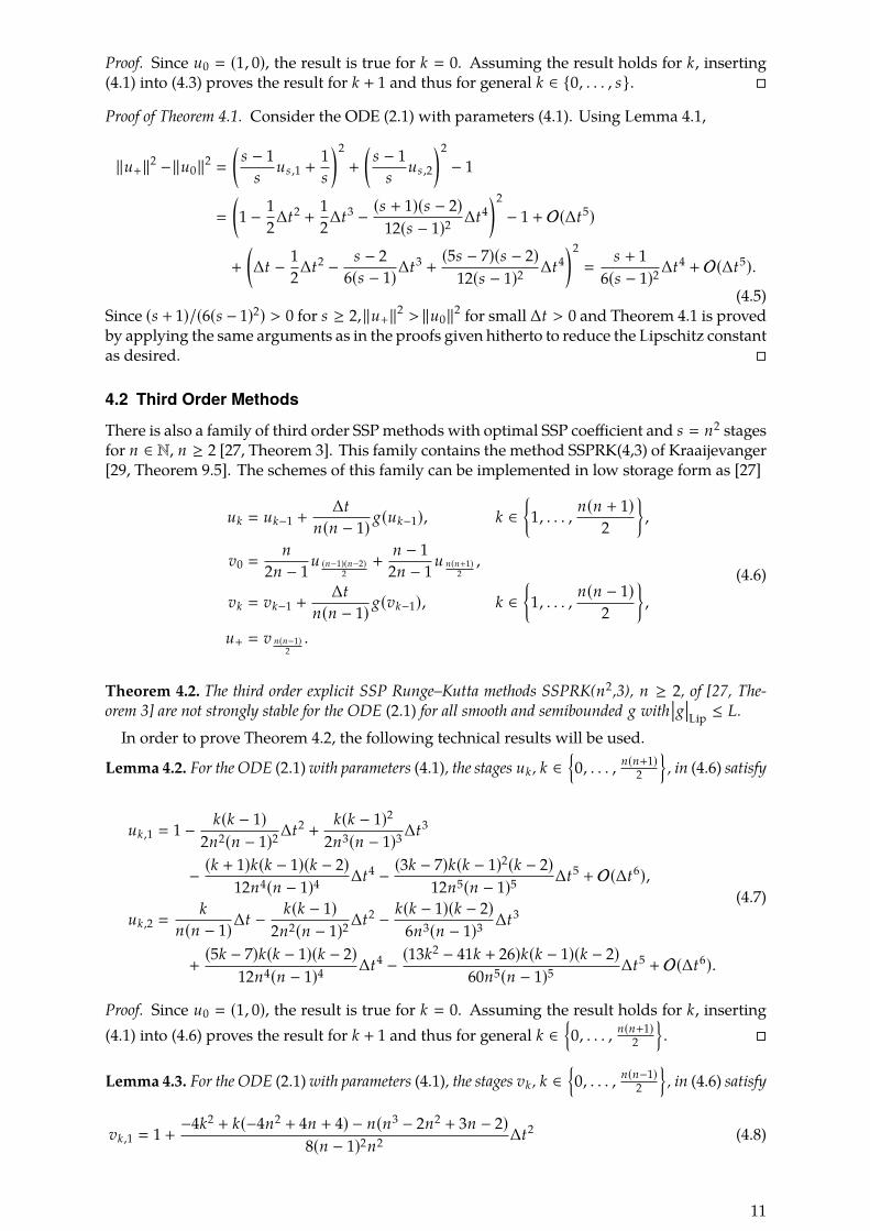
Proof. Since u0 � (1, 0), the result is true for k � 0. Assuming the result holds for k, inserting(4.1) into (4.3) proves the result for k + 1 and thus for general k ∈ {0, . . . , s}. �

Proof of Theorem 4.1. Consider the ODE (2.1) with parameters (4.1). Using Lemma 4.1,

‖u+‖2 −‖u0‖2 �

(s − 1

sus ,1 +

1s

)2

+

(s − 1

sus ,2

)2

− 1

�

(1 − 1

2∆t2+

12∆t3 − (s + 1)(s − 2)

12(s − 1)2 ∆t4)2

− 1 + O(∆t5)

+

(∆t − 1

2∆t2 − s − 26(s − 1)∆t3

+(5s − 7)(s − 2)

12(s − 1)2 ∆t4)2

�s + 1

6(s − 1)2∆t4+ O(∆t5).

(4.5)Since (s + 1)/(6(s − 1)2) > 0 for s ≥ 2,‖u+‖2 > ‖u0‖2 for small ∆t > 0 and Theorem 4.1 is provedby applying the same arguments as in the proofs given hitherto to reduce the Lipschitz constantas desired. �

4.2 Third Order Methods

There is also a family of third order SSPmethods with optimal SSP coefficient and s � n2 stagesfor n ∈ N, n ≥ 2 [27, Theorem 3]. This family contains the method SSPRK(4,3) of Kraaijevanger[29, Theorem 9.5]. The schemes of this family can be implemented in low storage form as [27]

uk � uk−1 +∆t

n(n − 1) g(uk−1), k ∈{1, . . . , n(n + 1)

2

},

v0 �n

2n − 1 u (n−1)(n−2)2

+n − 1

2n − 1 u n(n+1)2,

vk � vk−1 +∆t

n(n − 1) g(vk−1), k ∈{1, . . . , n(n − 1)

2

},

u+ � v n(n−1)2.

(4.6)

Theorem 4.2. The third order explicit SSP Runge–Kutta methods SSPRK(n2,3), n ≥ 2, of [27, The-orem 3] are not strongly stable for the ODE (2.1) for all smooth and semibounded g with

��g��Lip ≤ L.In order to prove Theorem 4.2, the following technical results will be used.

Lemma 4.2. For the ODE (2.1)with parameters (4.1), the stages uk , k ∈{0, . . . , n(n+1)

2

}, in (4.6) satisfy

uk ,1 � 1 − k(k − 1)2n2(n − 1)2∆t2

+k(k − 1)2

2n3(n − 1)3∆t3

− (k + 1)k(k − 1)(k − 2)12n4(n − 1)4 ∆t4 − (3k − 7)k(k − 1)2(k − 2)

12n5(n − 1)5 ∆t5+ O(∆t6),

uk ,2 �k

n(n − 1)∆t − k(k − 1)2n2(n − 1)2∆t2 − k(k − 1)(k − 2)

6n3(n − 1)3 ∆t3

+(5k − 7)k(k − 1)(k − 2)

12n4(n − 1)4 ∆t4 − (13k2 − 41k + 26)k(k − 1)(k − 2)60n5(n − 1)5 ∆t5

+ O(∆t6).

(4.7)

Proof. Since u0 � (1, 0), the result is true for k � 0. Assuming the result holds for k, inserting(4.1) into (4.6) proves the result for k + 1 and thus for general k ∈

{0, . . . , n(n+1)

2

}. �

Lemma 4.3. For the ODE (2.1)with parameters (4.1), the stages vk , k ∈{0, . . . , n(n−1)

2

}, in (4.6) satisfy

vk ,1 � 1 +−4k2 + k(−4n2 + 4n + 4) − n(n3 − 2n2 + 3n − 2)

8(n − 1)2n2 ∆t2 (4.8)

11

+

(8k3

+ 4k2(3n2 − 3n − 4) + 2k(3n4 − 6n3 − n2+ 4n + 4)

+ n(n5 − 3n4+ 11n3 − 17n2

+ 4n + 4)) 1

16(n − 1)3n3∆t3

+

(16k4

+ 32k3(n2 − n − 1) + 8k2(3n4 − 6n3 − 3n2+ 6n − 2)

+ 8k(n6 − 3n5+ 5n3

+ 3n2 − 6n + 4)+ n(n7 − 4n6

+ 26n5 − 64n4+ 57n3 − 12n2 − 20n + 16)

) 1192(n − 1)4n4∆t4

+

(96k5

+ 16k4(15n2 − 15n − 38) + 16k3(15n4 − 30n3 − 41n2+ 56n + 86)

+ 8k2(15n6 − 45n5+ 27n4

+ 21n3+ 96n2 − 114n − 164)

+ 2k(15n8 − 60n7+ 178n6 − 324n5

+ 11n4+ 448n3 − 284n2

+ 16n + 224)+ n(3n9 − 15n8

+ 112n7 − 358n6+ 247n5

+ 449n4 − 354n3 − 428n2+ 120n + 224)

)1

384(n − 1)5n5∆t5+ O(∆t6),

and

vk ,2 �2k + n2 − n2(n − 1)n ∆t +

−4k2 + k(−4n2 + 4n + 4) − n(n3 − 2n2 + 3n − 2)8(n − 1)2n2 ∆t2 (4.9)

−(8k3

+ 12k2(n2 − n − 2) + 2k(3n4 − 6n3+ 3n2

+ 8)

+ n(n5 − 3n4+ 9n3 − 13n2 − 2n + 8)

) 148(n − 1)3n3∆t3

+

(80k4

+ 32k3(5n2 − 5n − 11) + 8k2(15n4 − 30n3 − 27n2+ 42n + 62)

+ 8k(5n6 − 15n5+ 30n4 − 35n3

+ 21n2 − 6n − 28)+ n(5n7 − 20n6

+ 106n5 − 248n4+ 69n3

+ 252n2 − 52n − 112)) 1

192(n − 1)4n4∆t4

−(416k5

+ 80k4(13n2 − 13n − 32) + 80k3(13n4 − 26n3 − 39n2+ 52n + 70)

+ 40k2(13n6 − 39n5+ 15n4

+ 35n3+ 98n2 − 122n − 128)

+ 2k(65n8 − 260n7+ 950n6 − 1940n5

+ 725n4+ 1480n3 − 1500n2

+ 480n + 832)+ n(13n9 − 65n8

+ 490n7 − 1570n6+ 1165n5

+ 1727n4 − 1508n3 − 1564n2

+ 480n + 832)) 1

1920(n − 1)5n5∆t5+ O(∆t6).

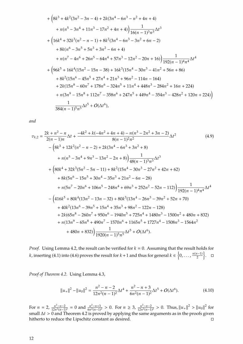
Proof. Using Lemma 4.2, the result can be verified for k � 0. Assuming that the result holds fork, inserting (4.1) into (4.6) proves the result for k +1 and thus for general k ∈

{0, . . . , n(n−1)

2

}. �

Proof of Theorem 4.2. Using Lemma 4.3,

‖u+‖2 −‖u0‖2 �n2 − n − 2

12n2(n − 1)2∆t4+

n2 − n + 36n2(n − 1)2∆t5

+ O(∆t6). (4.10)

For n � 2, n2−n−212n2(n−1)2 � 0 and n2−n+3

6n2(n−1)2 > 0. For n ≥ 3, n2−n−212n2(n−1)2 > 0. Thus, ‖u+‖2 > ‖u0‖2 for

small ∆t > 0 and Theorem 4.2 is proved by applying the same arguments as in the proofs givenhitherto to reduce the Lipschitz constant as desired. �

12

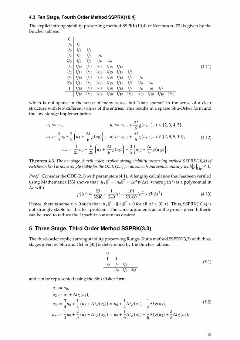
4.3 Ten Stage, Fourth Order Method SSPRK(10,4)

The explicit strong-stability preserving method SSPRK(10,4) of Ketcheson [27] is given by theButcher tableau

01/6 1/61/3 1/6 1/61/2 1/6 1/6 1/62/3 1/6 1/6 1/6 1/61/3 1/15 1/15 1/15 1/15 1/151/2 1/15 1/15 1/15 1/15 1/15 1/62/3 1/15 1/15 1/15 1/15 1/15 1/6 1/65/6 1/15 1/15 1/15 1/15 1/15 1/6 1/6 1/61 1/15 1/15 1/15 1/15 1/15 1/6 1/6 1/6 1/6

1/10 1/10 1/10 1/10 1/10 1/10 1/10 1/10 1/10 1/10

(4.11)

which is not sparse in the sense of many zeros, but “data sparse” in the sense of a clearstructure with few different values of the entries. This results in a sparse Shu-Osher form andthe low-storage implementation

u1 :� u0 , ui :� ui−1 +∆t6 g(ui−1), i ∈ {2, 3, 4, 5},

u6 :� 35 u0 +

25

(u5 +

∆t6 g(u5)

), ui :� ui−1 +

∆t6 g(ui−1), i ∈ {7, 8, 9, 10},

u+ :� 125 u0 +

925

(u5 +

∆t6 g(u5)

)+

35

(u10 +

∆t6 g(u10)

).

(4.12)

Theorem 4.3. The ten stage, fourth order, explicit strong stability preserving method SSPRK(10,4) ofKetcheson [27] is not strongly stable for the ODE (2.1) for all smooth and semibounded g with

��g��Lip ≤ L.

Proof. Consider theODE (2.1)withparameters (4.1). A lengthy calculation that hasbeenverifiedusing Mathematica [53] shows that ‖u+‖2 −‖u0‖2 � ∆t6p(∆t), where p(∆t) is a polynomial in∆t with

p(∆t) � 233240 −

1240∆t − 161

29160∆t2+ O(∆t3). (4.13)

Hence, there is some τ > 0 such that ‖u+‖2 −‖u0‖2 > 0 for all ∆t ∈ (0, τ). Thus, SSPRK(10,4) isnot strongly stable for this test problem. The same arguments as in the proofs given hithertocan be used to reduce the Lipschitz constant as desired. �

5 Three Stage, Third Order Method SSPRK(3,3)

The third-order explicit strong stability preserving Runge–Kuttamethod SSPRK(3,3) with threestages given by Shu and Osher [45] is determined by the Butcher tableau

01 1

1/2 1/4 1/41/6 1/6 2/3

(5.1)

and can be represented using the Shu-Osher form

u1 :� u0 ,

u2 :� u1 + ∆t g(u1),u3 :� 3

4 u0 +14

(u2 + ∆t g(u2)

)� u0 +

14∆t g(u1) + 1

4∆t g(u2),

u+ :� 13 u0 +

23

(u3 + ∆t g(u3)

)� u0 +

16∆t g(u1) + 1

6∆t g(u2) + 23∆t g(u3).

(5.2)

13

Theorem 3.2 implies that SSPRK(3,3) is not strongly stable for general semibounded g. Sincethis method is often used, it is considered for further stability investigations in this section. Inparticular, the following properties will be studied.

• The classical fourth order, four stage explicit Runge–Kutta method RK(4,4) is not stronglystable for general semibounded and linear g. However, the method given by two consec-utive steps of RK(4,4) is strongly stable for such g, cf. [47]. Thus, it is of interest whethersomething similar is true for SSPRK(3,3) for general nonlinear semibounded g.

• Even if SSPRK(3,3) is not strongly stable after a finite number of steps, the increase ofthe norm might still be bounded, cf. [23–25] for investigations of such a property whenthe explicit Euler method is assumed to be strongly stable. Although boundedness andmonotonicity are equivalent in this context for a large class of Runge–Kutta methods [25],this result cannot be applied here directly. Hence, it is of interest to study the behaviourof SSPRK(3,3) for semibounded g.

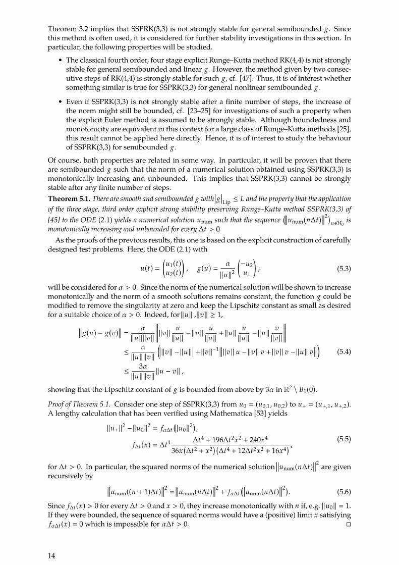
Of course, both properties are related in some way. In particular, it will be proven that thereare semibounded g such that the norm of a numerical solution obtained using SSPRK(3,3) ismonotonically increasing and unbounded. This implies that SSPRK(3,3) cannot be stronglystable after any finite number of steps.Theorem 5.1. There are smooth and semibounded g with

��g��Lip ≤ L and the property that the applicationof the three stage, third order explicit strong stability preserving Runge–Kutta method SSPRK(3,3) of[45] to the ODE (2.1) yields a numerical solution unum such that the sequence

( unum(n∆t) 2)n∈N0

ismonotonically increasing and unbounded for every ∆t > 0.As the proofs of the previous results, this one is based on the explicit construction of carefully

designed test problems. Here, the ODE (2.1) with

u(t) �(u1(t)u2(t)

), g(u) � α

‖u‖2(−u2

u1

), (5.3)

will be considered for α > 0. Since the norm of the numerical solutionwill be shown to increasemonotonically and the norm of a smooth solutions remains constant, the function g could bemodified to remove the singularity at zero and keep the Lipschitz constant as small as desiredfor a suitable choice of α > 0. Indeed, for ‖u‖ ,‖v‖ ≥ 1,

g(u) − g(v) �α

‖u‖‖v‖ ‖v‖ u

‖u‖ −‖u‖u‖u‖ +‖u‖

u‖u‖ −‖u‖

v‖v‖

≤ α‖u‖‖v‖

(��‖v‖ −‖u‖�� +‖v‖−1 ‖v‖ u −‖v‖ v +‖v‖ v −‖u‖ v )

≤ 3α‖u‖‖v‖ ‖u − v‖ ,

(5.4)

showing that the Lipschitz constant of g is bounded from above by 3α in R2 \ B1(0).Proof of Theorem 5.1. Consider one step of SSPRK(3,3) from u0 � (u0,1 , u0,2) to u+ � (u+,1 , u+,2).A lengthy calculation that has been verified using Mathematica [53] yields

‖u+‖2 −‖u0‖2 � fα∆t(‖u0‖2

),

f∆t(x) � ∆t4 ∆t4 + 196∆t2x2 + 240x4

36x(∆t2 + x2

) (∆t4 + 12∆t2x2 + 16x4

) , (5.5)

for ∆t > 0. In particular, the squared norms of the numerical solution unum(n∆t) 2 are given

recursively by unum((n + 1)∆t) 2� unum(n∆t) 2

+ fα∆t( unum(n∆t) 2)

. (5.6)

Since f∆t(x) > 0 for every∆t > 0 and x > 0, they increase monotonically with n if, e.g. ‖u0‖ � 1.If they were bounded, the sequence of squared norms would have a (positive) limit x satisfyingfα∆t(x) � 0 which is impossible for α∆t > 0. �

14

Numerical solutions of (5.3) with α � 1 and initial condition u0 � (1, 0) have been computedusing SSPRK(3,3) implemented in DifferentialEquations.jl [39] in Julia v1.1.0 [4] using usingfloating point numbers with extended precision (BigFloat with setprecision(500)). Asvisualised in Figure 1, the energy increases monotonically for every time step ∆t > 0, inaccordance with Theorem 5.1.

0.0 0.2 0.4 0.6 0.8 1.0t

10−22

10−20

10−18

10−16

10−14

10−12

10−10

||u(t)||2−||u

0||2

∆t � 10−3

∆t � 10−4∆t � 10−5

∆t � 10−6

Figure 1: Evolution of the energy of numerical solutions computed using SSPRK(3,3) with different timesteps ∆t.

Remark 5.1. In applications, only finite final times T > 0 are relevant. Hence, it can beinteresting whether a bound of the form

∀n ∈ N, n∆t ≤ T : u(n∆t) ≤ cT (5.7)

holds for some constant cT > 0 depending on T. For explicit schemes, a useful bound seemsto require an additional restriction of the time step ∆t because of stability issues. Choosing0 < ∆t < ∆tmax small enough, such a bound will trivially hold if the scheme converges.However, it does not seem to be trivial to guarantee good estimates of cT and∆tmax in general. /

6 Ten Stage, Fourth Order Method SSPRK(10,4) and the TransportEquation

In this section, themethod SSPRK(10,4) of [27] described in section 4.3will be used to integrate asemidiscretisation of a hyperbolic conservation law in time. Itwill be demonstrated numericallythat the energy (squared norm) of the solution increases for a wide range of positive time steps.Consider the linear advection equation with periodic boundary conditions

∂t u(t , x) + ∂x u(t , x) � 0, t ∈ (0, T), x ∈ (xL , xR),u(0, x) � u0(x), x ∈ (xL , xR),

u(t , xL) � u(t , xR), t ∈ (0, T),(6.1)

and the initial condition u0(x) � − sin(πx) in the domain (xL , xR) � (−1, 1). Using the L2

entropy U(u) � 12 u2, the entropy flux is F(u) � 1

2 u2 and the flux potential is ψ(u) � 12 u2.

Smooth solutions fulfil u(t) 2

2 � ‖u0‖22 and the entropy inequality

∂t u(t , x)2 + ∂x u(t , x)2 ≤ 0 (6.2)

yields u(t) 2

2 ≤ ‖u0‖22 for general solutions, cf. [50, 52].Recently, Abgrall [1] proposed a general method to make numerical schemes entropy con-

servative/stable. He described this approach using residual distribution schemes and explains

15

how some other frameworks can be recast in this way, see also [2, 3]. For nodal discontinuousGalerkin (DG) schemes in one space dimension, this approach will be adapted in the following.Consider a general polynomial collocation approach using p + 1 nodes and polynomials of

degree ≤ p in an element [xi−1 , xi]. Besides the choice of the nodes, the main ingredients are

• a mass matrix M , approximating the L2 scalar product via∫ xi

xi−1u(x)v(x)dx � 〈u , v〉L2 ≈⟨

u , v⟩

M � uT M v.

• a derivative matrix D , approximating the derivative ∂x u ≈ D u.

• a restriction operator R , performing interpolation to the boundary nodes xi−1 , xi viaR u � (uL , uR)T .

• a diagonal boundary matrix B � diag (−1, 1), giving the difference of boundary values asin the fundamental theorem of calculus.

If the mass matrix is exact for polynomials of degree ≤ 2p − 1, the summation by partsproperty

M D + DT M � RT B R (6.3)

will be satisfied, cf. [13, 16, 21]. In that case, semidiscrete stability can be proven in manycases, as described in the review articles of Fernández, Hicken and Zingg [14] and Svärd andNordström [49] and references cited therein.AnodalDGsemidiscretisationof the advection equation (6.1)will beperformedas follows. At

first, the domain (xL , xR) is divided uniformly into N non-overlapping elements. Each elementis mapped via an affine-linear mapping to the reference element (−1, 1) and all computationsare performed there. On each element, the semidiscretisation is

∂t u + D u � −M−1RT B(

f num − R u), (6.4)

where the numerical flux will be the central flux f num(u− , u+) � u−+u+

2 . This flux is entropyconservative for the L2 entropy U(u) � u2

2 . Thus, if SBP operators are used, e.g. via baseson Gauss or Lobatto Legendre nodes, the resulting semidiscretisation is entropy conservative.Indeed, using SBP operators yields

uT M ∂t u � −uT M D u − uT RT B(

f num − R u)

� −12 uT M D u − 1

2 uT RT B R u +12 uT DT M u − uT RT B

(f num − R u

)�

12 uT RT B R u − uT RT B f num ,

(6.5)

where the SBP property (6.3) has been used in the second line. Writing the element index as anupper index and suppressing the index ·(i) for the i-th element, this can be rewritten as

uT M ∂t u �12 uT RT B R u − uT RT B f num

�12

(u2

R − u2L

)−

(uR f num (

uR , u(i+1)L

) − uL f num (u(i−1)

R , uL) )

�©­«

u(i−1)R + uL

2 f num (u(i−1)

R , uL) − u2

L

2ª®¬− ©­«(uR + u(i+1)

L

2 f num (uR , u

(i+1)L

) − u2R

2ª®¬

� −1T R T B Fnum , Fnum�

(Fnum (

u(i−1)R , uL

), Fnum (

uR , u(i+1)L

) )T,

(6.6)

where Fnum(u− , u+) � (u− + u+)/2 · f num(u− , u+) − (ψ(u−) + ψ(u+))/2 is the entropy flux ofTadmor [52]. The basic idea of Abgrall [1] is to enforce (6.6) for any semidiscretisation via the

16

addition of a correction term r on the left hand side of (6.4) that is consistent with zero anddoes not violate the conservation relation (using D 1 � 0)

1T M ∂t u � −1T M D u − 1T RT B(

f num − R u)� −1T R T B f num. (6.7)

He proposes a correction term of the form

r � α©­«

u −1T M u

1T M 11ª®¬, α �

EuT M u − (1

T M u)21T M 1

,

E � 1T R T B Fnum − wT M D u − uT RT B(

f num − R u).

(6.8)

Indeed, the conservation relation (6.7) is left unchanged, since

1T M r � α©­«1T M u −

1T M u

1T M 11T M 1ª®¬

� 0. (6.9)

Moreover, the entropy rate satisfies the desired equation (6.6), since

uT M ∂t u � −uT M r − uT M D u − uT RT B(

f num − R u)�

� − α ©­«uT M u −

1T M u

1T M 1uT M 1ª®¬︸¨ ¨ ¨ ¨ ¨ ¨ ¨ ¨ ¨ ¨ ¨ ¨ ¨ ¨ ¨︷︷¨ ¨ ¨ ¨ ¨ ¨ ¨ ¨ ¨ ¨ ¨ ¨ ¨ ¨ ¨︸

�E

−uT M D u − uT RT B(

f num − R u)

� −1T R T B Fnum.

(6.10)

If the denominator of α in (6.8) is zero, the numerical solution is constant in the element becauseof the Cauchy Schwarz inequality (since 1 and u are linearly dependent in that case). Then, theDG scheme reduces to a finite volume scheme using the numerical flux f num and is thereforeentropy conservative/stable depending on f num.

In the following, some numerical experiments will be conducted using nodal DG methodson equidistant nodes including the boundaries and diagonal mass matrices using the weightsof the closed Newton Cotes quadrature formula (which are positive in the cases consideredbelow). The domain is divided into N � 16 elements and polynomials of degree ≤ p � 3 areapplied. The initial condition is advanced one time step ∆t using SSPRK(10,4) of [27].

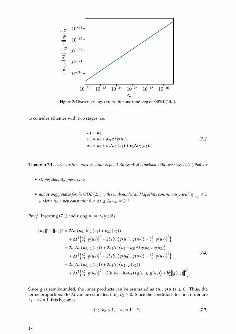
These methods have been implemented in Julia v0.6.4 [4] using floating point numberswith extended precision (BigFloat with setprecision(5000)). Using 500 different valuesof ∆t (with uniformly distributed logarithms), the discrete energy errors after one time step unum(∆t) 2

M −‖u0‖2M (computed via the mass matrix M ) are shown in Figure 2. As can be seenthere, the discrete energy increases for every choice of ∆t > 0. Moreover, the increase of theenergy scales as O(∆t5), as expected for one time step of a fourth order Runge–Kutta method.

To sum up, a semidiscrete DG scheme with insufficient quadrature strength is made semi-discretely energy conservative following the approach of Abgrall [1]. Integrating the resultingordinary differential equation in time with SSPRK(10,4) results in monotonically increasingenergies, even for ridiculously small time steps ∆t > 0.

7 First Order Schemes

In contrast to the negative results of the previous sections for explicit methods of at least secondorder of accuracy, there are first order schemes that are strongly stable. To prove this, it suffices

17

10−50 10−42 10−34 10−26 10−18 10−10

∆t

10−216

10−174

10−132

10−90

10−48

u num(∆

t) 2 M−‖

u 0‖2 M

Figure 2: Discrete energy errors after one time step of SSPRK(10,4).

to consider schemes with two stages, i.e.

u1 � u0 ,

u2 � u0 + a21∆t g(u1),u+ � u0 + b1∆t g(u1) + b2∆t g(u2).

(7.1)

Theorem 7.1. There are first order accurate explicit Runge–Kutta method with two stages (7.1) that are

• strong stability preserving

• and strongly stable for theODE (2.1)with semibounded and Lipschitz continuous g with��g��Lip ≤ L

under a time step constraint 0 < ∆t ≤ ∆tmax ∝ L−1.

Proof. Inserting (7.1) and using u1 � u0 yields

‖u+‖2 −‖u0‖2 � 2∆t⟨u0 , b1 g(u1) + b2 g(u2)

⟩+ ∆t2

(b2

1 g(u1)

2+ 2b1b2

⟨g(u1), g(u2)

⟩+ b2

2 g(u2)

2)

� 2b1∆t⟨u0 , g(u0)

⟩+ 2b2∆t

⟨u2 − a21∆t g(u0), g(u2)

⟩+ ∆t2

(b2

1 g(u0)

2+ 2b1b2

⟨g(u0), g(u2)

⟩+ b2

2 g(u2)

2)

� 2b1∆t⟨u0 , g(u0)

⟩+ 2b2∆t

⟨u2 , g(u2)

⟩+ ∆t2

(b2

1 g(u0)

2+ 2(b1b2 − b2a21)

⟨g(u0), g(u2)

⟩+ b2

2 g(u2)

2).

(7.2)

Since g is semibounded, the inner products can be estimated as⟨ui , g(ui)

⟩ ≤ 0. Thus, theterms proportional to ∆t can be estimated if b1 , b2 ≥ 0. Since the conditions for first order areb1 + b2 � 1, this becomes

0 ≤ b2 ≤ 1, b1 � 1 − b2. (7.3)

18

The terms multiplied by ∆t2 satisfy

b21 g(u0)

2+ 2(b1b2 − b2a21)

⟨g(u0), g(u2)

⟩+ b2

2 g(u2)

2

� b21 g(u0)

2+ 2(b1b2 − b2a21)

⟨g(u0), g(u0) + g(u2) − g(u0)

⟩+ b2

2 g(u0) + g(u2) − g(u0)

2

�(b2

1 + 2(b1b2 − b2a21) + b22) g(u0)

2

+ 2(b1b2 − b2a21 + b22)

⟨g(u0), g(u2) − g(u0)

⟩+ b2

2 g(u2) − g(u0)

2

≤ ((b1 + b2)2 − 2b2a21) g(u0)

2

+ 2���b1b2 − b2a21 + b2

2

��� g(u0) g(u2) − g(u0)

+ b22 g(u2) − g(u0)

2

≤ ((b1 + b2)2 − 2b2a21) g(u0)

2

+ 2���b1b2 − b2a21 + b2

2

���|a21 | L∆t g(u0)

2+ b2

2a221L2∆t2 g(u0)

2.

(7.4)Inserting the order condition (7.3), the last expression can be written as

· · · ≤ (1 − 2b2a21) g(u0)

2+ 2|1 − a21 | |b2a21 | L∆t

g(u0) 2

+ |b2a21 |2 L2∆t2 g(u0) 2. (7.5)

If g(u0) � 0, then u+ � u2 � u1 � u0 and strong stability is obvious. Otherwise, the termwithout ∆t is negative if

1 − 2b2a21 < 0. (7.6)In that case, strong stability is achieved for sufficiently small ∆t (and the natural assumptionb2a21L , 0), since

(1 − 2b2a21) + 2|1 − a21 | |b2a21 | L∆t + |b2a21 |2 L2∆t2 ≤ 0 (7.7)

for

∆t ≤√(1 − a21)2 − (1 − 2b2a21) −|1 − a21 |

|b2a21 | L . (7.8)

Thus, there are strongly stable schemes.Choosing for example

b1 � b2 �12 , a21 �

32 , (7.9)

the new value u+ can be written as

u+ � u0 +12∆t g(u0) + 1

2∆t g(u2)

�34 u0 +

12∆t g(u0) + 1

4

(u2 − 3

2∆t g(u0))+

12∆t g(u2)

�34

(u0 +

16∆t g(u0)

)+

14

(u2 + 2∆t g(u2)

).

(7.10)

Since u2 � u0 +32∆t g(u0), u+ is a convex combination of explicit Euler steps with positive step

sizes, the resulting scheme is strong stability preserving. �

Remark 7.1. Of course, the scheme constructed in the proof of Theorem 7.1 and the derivedlower bound on the SSP coefficient are not optimal. However, since such first order schemesare not really relevant in practice, no attempt to optimise them has been made. /

Remark 7.2. Generalising the approach used in proof of Theorem 7.1, it can be expected thatthere are strongly stable schemes of first order if more stages are used. /

Remark 7.3. If a non-autonomous problem (2.8) is considered, the proof of Theorem7.1 requiresLipschitz continuity in (t , u) instead of continuity in t and Lipschitz continuity in u as requiredfor the Picard-Lindelöf theorem, since f (t2 , u2) − f (t0 , u0) has to be estimated. /

Remark 7.4. Since higher-order schemes satisfy‖u+‖2−‖u0‖2 � O(∆tp) for p > 2 if g is smooth,it does not seem to be (easily) possible to get similar estimate for higher order schemes usingonly Lipschitz continuity of g. /

19

8 Summary and Discussion

In this article, strong stability of explicit SSP Runge–Kutta methods has been investigated.Many well-known and widespread high order schemes are not strongly stable for ODEs withgeneral nonlinear, smooth, and semibounded operators with bounded Lipschitz constant, cf.Theorems 3.3, 4.1, 4.2, and 4.3. Moreover, it has been proven that the norms of the numericalsolutions can even increase monotonically and without bounds for the popular three stage,third order method SSPRK(3,3) of [45], cf. Theorem 5.1. Additionally, it has been shown insection 6 that the ten stage, fourth order method SSPRK(10,4) of [27] can result in increasingnorms of the solution for an energy stable and nonlinear semidiscretisation of a hyperbolicconservation law. Finally, it has been proven that such restrictions do not apply to first orderRunge–Kutta methods, cf. Theorem 7.1. In particular, there are strongly stable SSP methods,even for nonlinear and semibounded operators that are Lipschitz continuous. In that case,strong stability can be guaranteed under a time step restriction ∆t ≤ ∆tmax, where ∆tmax isproportional to the inverse of the Lipschitz constant of the right hand side.It is well-known that implicit Runge–Kutta methods can have more favourable stability

properties than explicit ones. In particular, there are strongly stable methods for generalsemibounded operators [7, sections 357–359]. Furthermore, summation by parts operators canbe used to construct schemes with these properties [5, 34, 38], resulting e.g. in energy stableschemes for nonlinear equations [37]. This is also related to space-time discontinuous Galerkinschemes, where entropy stability can be obtained [15].In this light, it seems interesting to investigatewhether there are general possibilities to obtain

strong stability of explicit Runge–Kutta methods by approximating the original problem, e.g.by adding sufficient artificial dissipation, cf. [54]. In the light of the current results, it mightbe conjectured that such a dissipative mechanism might be necessary to obtain strong stabilitywith explicit methods. If this is possible, it is interesting to compare such schemes with fullyimplicit ones.

Acknowledgements

The author was supported by the German Research Foundation (DFG, Deutsche Forschungs-gemeinschaft) under Grant SO 363/14-1. The author would like to thank David Ketchesonvery much for some comments on an earlier draft of this manuscript and for pointing out thereferences [11, 12].

References

[1] R. Abgrall. ‘A general framework to construct schemes satisfying additional conserva-tion relations. Application to entropy conservative and entropy dissipative schemes’. In:Journal of Computational Physics 372 (2018), pp. 640–666. doi: 10.1016/j.jcp.2018.06.031. arXiv: 1711.10358 [math.NA].

[2] R. Abgrall. Some remarks about conservation for residual distribution schemes. 2017. arXiv:1708.03108 [math.NA].

[3] R. Abgrall, E. le Mélédo and P. Öffner. On the Connection between Residual DistributionSchemes and Flux Reconstruction. 2018. arXiv: 1807.01261 [math.NA].

[4] J. Bezanson, A. Edelman, S. Karpinski and V. B. Shah. ‘Julia: A Fresh Approach to Nu-merical Computing’. In: SIAM Review 59.1 (2017), pp. 65–98. doi: 10.1137/141000671.arXiv: 1411.1607 [cs.MS].

[5] P. D. Boom and D. W. Zingg. ‘High-order implicit time-marching methods based ongeneralized summation-by-parts operators’. In: SIAM Journal on Scientific Computing 37.6(2015), A2682–A2709. doi: 10.1137/15M1014917.

20

[6] K. Burrage and J. C. Butcher. ‘Non-linear stability of a general class of differential equa-tion methods’. In: BIT Numerical Mathematics 20.2 (1980), pp. 185–203. doi: 10.1007/BF01933191.

[7] J. C. Butcher.Numerical Methods for Ordinary Differential Equations. Chichester: JohnWiley& Sons Ltd, 2016.

[8] M. H. Carpenter, D. Gottlieb and S. Abarbanel. ‘Time-Stable Boundary Conditions forFinite-Difference Schemes SolvingHyperbolic Systems:Methodology andApplication toHigh-Order Compact Schemes’. In: Journal of Computational Physics 111.2 (1994), pp. 220–236. doi: 10.1006/jcph.1994.1057.

[9] M. H. Carpenter, J. Nordström and D. Gottlieb. ‘A Stable and Conservative InterfaceTreatment of Arbitrary Spatial Accuracy’. In: Journal of Computational Physics 148.2 (1999),pp. 341–365. doi: 10.1006/jcph.1998.6114.

[10] G. Cooper. ‘Stability of Runge-Kutta Methods for Trajectory Problems’. In: IMA Journalof Numerical Analysis 7.1 (1987), pp. 1–13. doi: 10.1093/imanum/7.1.1.

[11] G. Dahlquist and R. Jeltsch. Generalized disks of contractivity for explicit and implicit Runge-Kuttamethods. Technical Report TRITA-NA-7906.Departement ofNumericalAnalysis andComputing Sciences, The Royal Institute of Technology, S-100 44 Stockholm 70, Sweden:Institut för Numerisk Analysis, KTH Stockholm, Jan. 1979.

[12] K. Dekker and J. G. Verwer. Stability of Runge-Kutta methods for stiff nonlinear differentialequations. Vol. 2. CWI Monographs. Amsterdam: North-Holland, 1984.

[13] D. C. D. R. Fernández, P. D. Boom and D. W. Zingg. ‘A generalized framework for nodalfirst derivative summation-by-parts operators’. In: Journal of Computational Physics 266(2014), pp. 214–239. doi: 10.1016/j.jcp.2014.01.038.

[14] D. C. D. R. Fernández, J. E. Hicken and D. W. Zingg. ‘Review of summation-by-partsoperators with simultaneous approximation terms for the numerical solution of partialdifferential equations’. In: Computers & Fluids 95 (2014), pp. 171–196. doi: 10.1016/j.compfluid.2014.02.016.

[15] L. Friedrich, G. Schnücke, A. R. Winters, D. C. D. R. Fernández, G. J. Gassner and M. H.Carpenter. Entropy Stable Space-Time Discontinuous Galerkin Schemes with Summation-by-Parts Property for Hyperbolic Conservation Laws. 2018. arXiv: 1808.08218 [math.NA].

[16] G. J. Gassner. ‘A Skew-Symmetric Discontinuous Galerkin Spectral Element Discretiza-tion and Its Relation to SBP-SAT Finite Difference Methods’. In: SIAM Journal on ScientificComputing 35.3 (2013), A1233–A1253. doi: 10.1137/120890144.

[17] S. Gottlieb, D. I. Ketcheson and C.-W. Shu. Strong stability preserving Runge-Kutta andmultistep time discretizations. Singapore: World Scientific, 2011.

[18] B. Gustafsson, H.-O. Kreiss and J. Oliger. Time-Dependent Problems and Difference Methods.Hoboken: John Wiley & Sons, 2013.

[19] E. Hairer, C. Lubich and G. Wanner. Geometric Numerical Integration: Structure-PreservingAlgorithms for Ordinary Differential Equations. Vol. 31. Springer Series in ComputationalMathematics. Berlin Heidelberg: Springer-Verlag, 2006. doi: 10.1007/3-540-30666-8.

[20] E. Hairer, S. P. Nørsett and G. Wanner. Solving Ordinary Differential Equations I: Non-stiff Problems. Vol. 8. Springer Series in Computational Mathematics. Berlin Heidelberg:Springer-Verlag, 2008. doi: 10.1007/978-3-540-78862-1.

[21] J. E.Hicken andD.W.Zingg. ‘Summation-by-parts operators andhigh-order quadrature’.In: Journal of Computational and Applied Mathematics 237.1 (2013), pp. 111–125. doi: 10.1016/j.cam.2012.07.015.

[22] I. Higueras. ‘Monotonicity for Runge-Kutta Methods: Inner Product Norms’. In: Journalof Scientific Computing 24.1 (2005), pp. 97–117. doi: 10.1007/s10915-004-4789-1.

21

[23] W. Hundsdorfer, A. Mozartova and M. N. Spijker. ‘Special boundedness properties innumerical initial value problems’. In: BIT Numerical Mathematics 51.4 (2011), pp. 909–936.doi: 10.1007/s10543-011-0349-x.

[24] W. Hundsdorfer, A. Mozartova and M. N. Spijker. ‘Stepsize conditions for boundednessin numerical initial value problems’. In: SIAM Journal on Numerical Analysis 47.5 (2009),pp. 3797–3819. doi: 10.1137/090745842.

[25] W. Hundsdorfer and M. N. Spijker. ‘Boundedness and strong stability of Runge-Kuttamethods’. In:Mathematics of Computation 80.274 (2011), pp. 863–886. doi: 10.1090/S0025-5718-2010-02422-6.

[26] H. T. Huynh. ‘A Flux Reconstruction Approach to High-Order Schemes Including Dis-continuous Galerkin Methods’. In: 18th AIAA Computational Fluid Dynamics Conference.American Institute of Aeronautics and Astronautics. AIAA, 2007. doi: 10.2514/6.2007-4079.

[27] D. I. Ketcheson. ‘Highly Efficient Strong Stability-Preserving Runge-Kutta Methods withLow-Storage Implementations’. In: SIAM Journal on Scientific Computing 30.4 (2008),pp. 2113–2136. doi: 10.1137/07070485X.

[28] D. A. Kopriva and E. Jimenez. ‘An Assessment of the Efficiency of Nodal DiscontinuousGalerkin Spectral Element Methods’. In: Recent Developments in the Numerics of NonlinearHyperbolic Conservation Laws. Ed. by R. Ansorge, H. Bijl, A. Meister and T. Sonar. Berlin:Springer Berlin Heidelberg, 2013, pp. 223–235. doi: 10.1007/978-3-642-33221-0_13.

[29] J. F. B. M. Kraaijevanger. ‘Contractivity of Runge-Kutta methods’. In: BIT NumericalMathematics 31.3 (1991), pp. 482–528. doi: 10.1007/BF01933264.

[30] H.-O. Kreiss and J. Lorenz. Initial-Boundary Value Problems and the Navier-Stokes Equations.Vol. 47. Classics in Applied Mathematics. Philadelphia: SIAM, 2004.

[31] H.-O. Kreiss and G. Scherer. ‘Finite Element and Finite Difference Methods for Hyper-bolic Partial Differential Equations’. In: Mathematical Aspects of Finite Elements in PartialDifferential Equations. Ed. by C. de Boor. New York: Academic Press, 1974, pp. 195–212.

[32] D. Levy and E. Tadmor. ‘From Semidiscrete to Fully Discrete: Stability of Runge-KuttaSchemes by The Energy Method’. In: SIAM Review 40.1 (1998), pp. 40–73. doi: 10.1137/S0036144597316255.

[33] C. Lozano. ‘Entropy Production by Explicit Runge-Kutta Schemes’. In: Journal of ScientificComputing 76.1 (2018), pp. 521–565. doi: 10.1007/s10915-017-0627-0.

[34] T. Lundquist and J. Nordström. ‘The SBP-SAT technique for initial value problems’. In:Journal of Computational Physics 270 (2014), pp. 86–104. doi: 10.1016/j.jcp.2014.03.048.

[35] J. Nordström andM. Björck. ‘Finite volume approximations and strict stability for hyper-bolic problems’. In: Applied Numerical Mathematics 38.3 (2001), pp. 237–255. doi: 10.1016/S0168-9274(01)00027-7.

[36] J. Nordström, K. Forsberg, C. Adamsson and P. Eliasson. ‘Finite volume methods, un-structured meshes and strict stability for hyperbolic problems’. In: Applied NumericalMathematics 45.4 (2003), pp. 453–473. doi: 10.1016/S0168-9274(02)00239-8.

[37] J. Nordström and C. La Cognata. ‘Energy stable boundary conditions for the nonlinearincompressible Navier-Stokes equations’. In: Mathematics of Computation (2018). doi: 10.1090/mcom/3375.

[38] J. Nordström and T. Lundquist. ‘Summation-by-parts in time’. In: Journal of ComputationalPhysics 251 (2013), pp. 487–499. doi: 10.1016/j.jcp.2013.05.042.

[39] C. Rackauckas and Q. Nie. ‘DifferentialEquations.jl – A Performant and Feature-RichEcosystem for Solving Differential Equations in Julia’. In: Journal of Open Research Software5.1 (2017), p. 15. doi: 10.5334/jors.151.

[40] A. Ralston. ‘Runge-Kutta methods with minimum error bounds’. In:Mathematics of Com-putation 16.80 (1962), pp. 431–437. doi: 10.1090/S0025-5718-1962-0150954-0.

22

[41] H. Ranocha. StrongStabilityExplicitRungeKuttaForNonlinearOperators. On Strong Stability ofExplicit Runge–KuttaMethods forNonlinear SemiboundedOperators. https://github.com/ranocha/StrongStabilityExplicitRungeKuttaForNonlinearOperators.Nov. 2018. doi: 10.5281/zenodo.3066828.

[42] H. Ranocha and P. Öffner. ‘L2 Stability of Explicit Runge-Kutta Schemes’. In: Journal ofScientific Computing 75.2 (May 2018), pp. 1040–1056. doi: 10.1007/s10915-017-0595-4.

[43] H. Ranocha, P. Öffner and T. Sonar. ‘Summation-by-parts operators for correction proced-ure via reconstruction’. In: Journal of Computational Physics 311 (Apr. 2016), pp. 299–328.doi: 10.1016/j.jcp.2016.02.009. arXiv: 1511.02052 [math.NA].

[44] J. T. Schwartz. Nonlinear functional analysis. Vol. 4. Notes on Mathematics and its Applic-ations. New York: Gordon and Breach Science Publishers Inc., 1969.

[45] C.-W. Shu and S. Osher. ‘Efficient implementation of essentially non-oscillatory shock-capturing schemes’. In: Journal of Computational Physics 77.2 (1988), pp. 439–471. doi:10.1016/0021-9991(88)90177-5.

[46] G. Söderlind. ‘The logarithmic norm. History and modern theory’. In: BIT NumericalMathematics 46.3 (2006), pp. 631–652. doi: 10.1007/s10543-006-0069-9.

[47] Z. Sun and C.-W. Shu. ‘Stability of the fourth order Runge-Kutta method for time-dependent partial differential equations’. In: Annals of Mathematical Sciences and Ap-plications 2.2 (2017), pp. 255–284. doi: 10.4310/AMSA.2017.v2.n2.a3. url: https:/ / www . brown . edu / research / projects / scientific - computing / sites / brown .edu.research.projects.scientific-computing/files/uploads/Stability%20of%20the%20fourth%20order%20Runge- Kutta%20method%20for%20time- dependent%20partial.pdf.

[48] Z. Sun and C.-W. Shu. Strong Stability of Explicit Runge-Kutta Time Discretizations. Submit-ted to SIAM Journal on Numerical Analysis. Nov. 2018. arXiv: 1811.10680 [math.NA].

[49] M. Svärd and J.Nordström. ‘Reviewof summation-by-parts schemes for initial-boundary-value problems’. In: Journal of Computational Physics 268 (2014), pp. 17–38. doi: 10.1016/j.jcp.2014.02.031.

[50] E. Tadmor. ‘Entropy stability theory for difference approximations of nonlinear conserva-tion laws and related time-dependent problems’. In:Acta Numerica 12 (2003), pp. 451–512.doi: 10.1017/S0962492902000156.

[51] E. Tadmor. ‘From Semidiscrete to Fully Discrete: Stability of Runge-Kutta Schemes bythe Energy Method II’. In: Collected Lectures on the Preservation of Stability under Discretiz-ation. Ed. by D. J. Estep and S. Tavener. Vol. 109. Proceedings in Applied Mathematics.Philadelphia: Society for Industrial and Applied Mathematics, 2002, pp. 25–49.

[52] E. Tadmor. ‘The numerical viscosity of entropy stable schemes for systems of conservationlaws. I’. In: Mathematics of Computation 49.179 (1987), pp. 91–103. doi: 10.1090/S0025-5718-1987-0890255-3.

[53] Wolfram Research, Inc. ‘Mathematica 10.3’. https://www.wolfram.com. 2015.[54] H. Zakerzadeh and U. S. Fjordholm. ‘High-order accurate, fully discrete entropy stable

schemes for scalar conservation laws’. In: IMA Journal of Numerical Analysis 36.2 (2016),pp. 633–654. doi: 10.1093/imanum/drv020.

23