On the Apparent Transparency of a Motion Blurred Object

Alessandro Giusti Vincenzo CagliotiDipartimento di Elettronica e Informazione, Politecnico di Milano

P.za Leonardo da Vinci, 32 20133 Milano – Italyalessandro.giusti@polimi.it vincenzo.caglioti@polimi.it

Abstract

An object which moves during the exposure time resultsin a blurred smear in the image. We consider the smear asif it was the image of a semitransparent object, and we re-trieve its alpha matte by means of known techniques. Ourwork is focused on the qualitative and quantitative anal-ysis of the alpha matte: in particular, we show that thealpha value at a pixel represents the fraction of the expo-sure time during which the object image overlapped thatpixel; then, we prove that the alpha matte enjoys a numberof properties, which can be used to derive constraints onthe object’s apparent contour, and its motion, from a singlemotion-blurred image. We show that some of these proper-ties also hold on the original image. We point out possibleapplications, and experimental results both on synthetic andreal finite-exposure images.

1. IntroductionWhen a moving object is photographed by a still camera,

its image is motion blurred because the object’s projectionon the image plane changes during the exposure time. Ifthe exposure time is not short enough in relation to the mo-tion speed, the object results in a visible, semitransparent“smear” or “streak” in the image, and its contours blendwith the background confusing traditional computer visiontechniques.

In this paper, we provide a meaningful interpretation ofthe smear’s alpha matte (i.e., transparency), which can berecovered by means of controlled shooting conditions orknown matting algorithms. Then, we prove that the alphamatte of the blurred object image enjoys several properties,which are linked to the object’s apparent contour and itsmotion during the exposure time.

Other than generically supporting the understanding ofthe object smear, this allows us to retrieve:

• the apparent contour at the beginning and end of theexposure;

• parts of the contour at arbitrary time instants inside theexposure time;

• envelopes of the moving contour;

• the path of corners on the contour;

• speed discontinuities of the contour, caused for exam-ple by impacts of the moving object.

Most literature dealing with motion blur is concernedwith removing it (“deblurring”), either assuming that it af-fects the whole image because of camera shake [5, 19], oraiming at deblurring moving objects [9]. In [8], the study ofthe blurred object’s alpha matte is used for recovering thepoint spread function, improving deblurring performance.

In our setting, on the contrary, we want to take advantageof the additional information that a single motion blurredimage incorporates about the scene structure and evolution,which can not be extracted from a single still image. Severalworks in literature follow a similar approach: [12, 14] esti-mate the speed of a moving vehicle and of a moving ball,respectively; in [10], rotational blur estimation is the basisfor a visual gyroscope, and [13] exploits motion blur to ob-tain depth information from a single blurred image. In [4]motion blur is used for joint reconstruction of geometry andphotometry of scenes with multiple moving objects.

Instead of referring to a specific application, our workhas a general validity when moving objects are imaged froma still camera, and provides a sound theoretical founda-tion for interpreting and extracting information from blurredsmears; contrarily to most works in the field, we use a gen-eral blur model, and do not require that blur is representablein the frequency domain. This allows us to handle any typeof motion.

The paper is structured as follows: at the beginning werecall a general model for motion-blurred image forma-tion (section 2), and show how the smear’s transparencycan be meaningfully interpreted in this context; we brieflyshow how transparency can be recovered under varyingconstraints, then introduce our notation and basic proper-ties. In section 3 we introduce and prove our main results,

1

which relate features on the alpha matte to meaningful con-straints on the moving object’s apparent contours during theexposure time. We discuss practical applications of our the-ory in section 4, whereas Section 5 presents experimentalresults on both real and synthetic images. Finally, we pro-vide conclusions and list future works (section 6).

2. Model and definitionsWe begin by presenting a model for the image of a mov-

ing object, highlighting the connections to the matting prob-lem by introducing the α(p) quantity, which will be ourmain object of study in the following.

2.1. Motion blur model and its relation with alphamatting

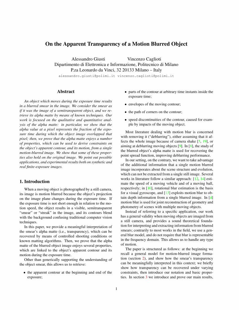
Figure 1. The image C of the motion blurred object can be inter-preted as the temporal average over the exposure time of infinitestill images It (top). We show that the blurred smear can be inter-preted as a semitransparent layer, whose alpha matte we analyzein the following.

A motion blurred image is obtained when the scene pro-jection on the image plane changes during the camera ex-posure period [t′, t′′]. The final image C is obtained as theintegration of infinite sharp images, each exposed for an in-finitesimal portion of [t′, t′′]. In an equivalent interpreta-tion (figure 1), we can consider the motion blurred image asthe temporal average of infinite sharp images It, each takenwith the same exposure time t′′ − t′ but representing thescene frozen at a different instant t ∈ [t′, t′′]. This tech-nique is also implemented in many 3D rendering packagesfor accurate synthesis of motion blurred images.

If the camera is static and a single object is moving inthe scene, the static background in the final image is sharpsince its pixels are of constant intensity in each It; con-versely, the image pixels which are affected by the movingobject, possibly only in some of the It images, belong to themotion-blurred image (smear) of the object.

For a pixel p, define i(p) ⊆ [t′, t′′] the set of time instantsduring which p belongs to the object image. We finally de-fine α(p) as the fraction of [t′, t′′] during which the objectprojects to p:

α(p) = ||i(p)||/(t′′ − t′). (1)

Let B(p) be the intensity of the background at p. SinceC is the temporal average of all the It images, C(p) =α(p)o(p) + (1 − α(p))B(p). o(p) is the temporal averageover i(p) of the intensity of image pixel C(p):

o(p) =1

||i(p)||

∫t∈i(p)

It(p) dt. (2)

To sum up, the intensity of a pixel p in the motion blurredimage C can be interpreted as the convex linear combina-tion of two factors: the ”object” intensity o(p), weightedα(p), and the background intensity. The resulting equationis the well-known Porter-Duff alpha compositing equation[16] for a pixel with transparency α(p) and intensity o(p)over the background pixel B(p). Recovering α(p) from amotion-blurred image is therefore equivalent to the well-known layer extraction (or alpha matting) problem.

2.2. Recovery of the alpha matte

If the object appears with a given constant intensity ona known background, α(p) can be readily derived at eachpixel by solving a first-degree linear equation.

In a color image, we can extend our considerations to allchannels separately, noting that α(p) is constant along allthe channels:

Cr(p) = α(p)or(p) + (1− α(p))Br(p)Cg(p) = α(p)og(p) + (1− α(p))Bg(p)Cb(p) = α(p)ob(p) + (1− α(p))Bb(p).

(3)

Then, if the background is known and the object colors meetsome constraints, α(p) can analytically be computed in thewhole image [7].

In the general case, the matting problem is undercon-strained, even if the background is known: still, in literaturemany algorithms have been proposed : some ([20, 15]) re-quire a specific background (blue screen matting), whereasothers ([2, 3, 17, 21, 11, 1]), with minimal user assistance,handle unknown backgrounds (natural image matting) andlarge zones of mixed pixels (0 < α < 1). Although none isexplicitly designed for the interpretation of blurred smears,we can get satisfactory results in our peculiar setting. As we

show in this paper, the alpha matte of blurred smears enjoyssome rather restrictive properties, and several constraintscan also be enforced for the object color: these additionalconstraints could be integrated in existing algorithms in thefuture, for a more accurate extraction of the alpha matte ofblurred smears.

As we discuss in section 4.2, some of our results alsohold for the original blurred image, which allows applica-tions even without matting.

2.3. Definitions, basic assumptions and properties

During the exposure time [t′, t′′], the object contourchanges. Let c(t) be the object apparent contour at t.

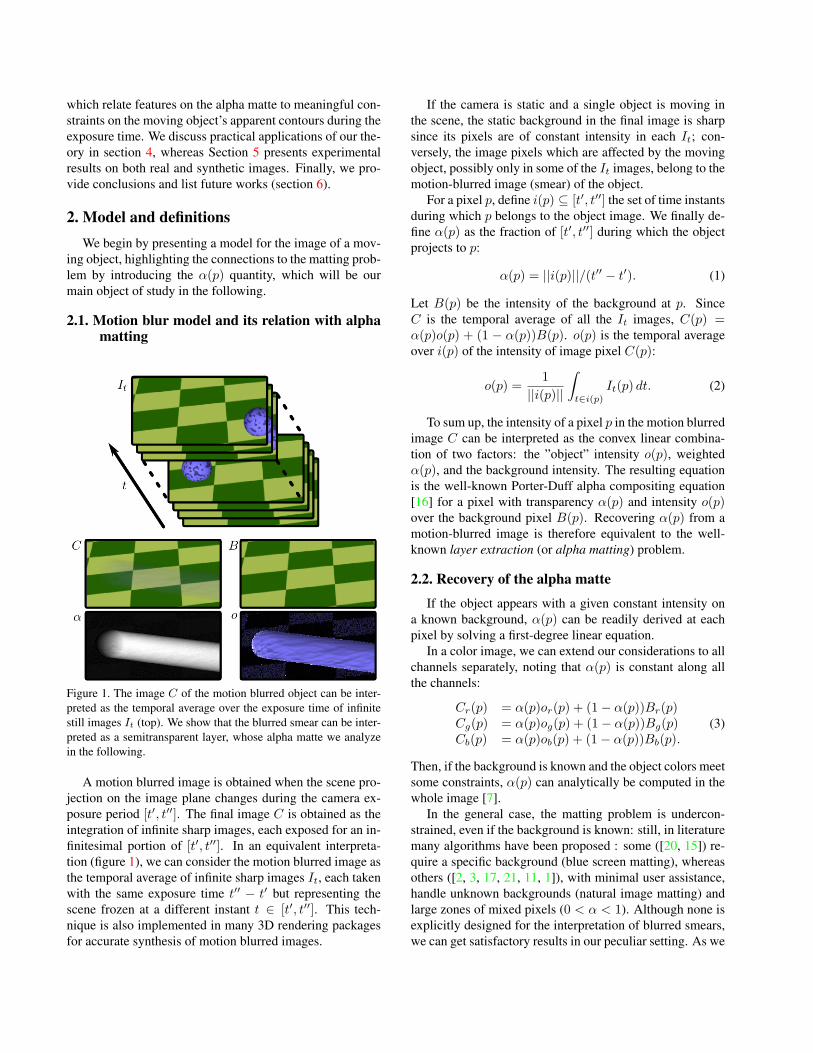
We partition the image in regions, which we classify onthe basis of two criteria:

• Whether the region is inside c(t′) (R•) or not (R◦),which we indicate with a superscript.

• How many times each image point belonging to theregion is crossed by c during the exposure time, whichwe indicate with a subscript.

Figure 2. The smear of a rotating object and its regions.

The background (α(p) = 0) is the R◦0 region. On the

contrary, the R•0 region is composed by all and only the

pixels covered by the object during the whole exposure(α = 1); in figure 2, there is no R•

0 region.Note that if any point inside c(t′) is crossed once by the

apparent contour, it will be outside c(t′′), and vice-versa;this is easily generalized to the following property.

Property 1. An R•2n+1 or R◦

2n region is outside c(t′′). AnR•

2n or R◦2n+1 region is inside c(t′′).

3. Properties of the blurred smear alpha matte

We present a meaningful property of α values in R1 re-gions, then discuss region topology and classify borders be-tween regions. Finally, we show how this relates to the al-pha matte.

3.1. α inside R1 regions

Theorem 2. The iso-α curve α = α within an R•1 region is

part of the apparent contour c(t′ + α(t′′ − t′)). Similarly,the iso-α curve α = α within an R◦

1 region is part of c(t′′−α(t′′ − t′)).

Proof. Each pixel p belongs to the object image for ex-actly α(p)(t′′ − t′) seconds. In an R•

1 region each pixelis crossed once by the object contour, therefore it belongsto the object image during a compact time interval startingat t′ and ending when it is crossed by the object contour, attime t′ + α(p)(t′′ − t′). The first part of the thesis immedi-ately follows. A similar argument holds for the second partof the thesis.

Corollary. In an R1 region the direction of ∇α(p) is or-thogonal to the object contour in p at time α(p)(t′′ − t′);|∇α(p)| is inversely proportional to the apparent contourmotion speed component along the direction of ∇α(p). Inan R◦

1 region ∇α(p) points towards the motion direction,whereas in R•

1, ∇α(p) points towards the opposite direc-tion.

3.2. Space-time representation of c(t)

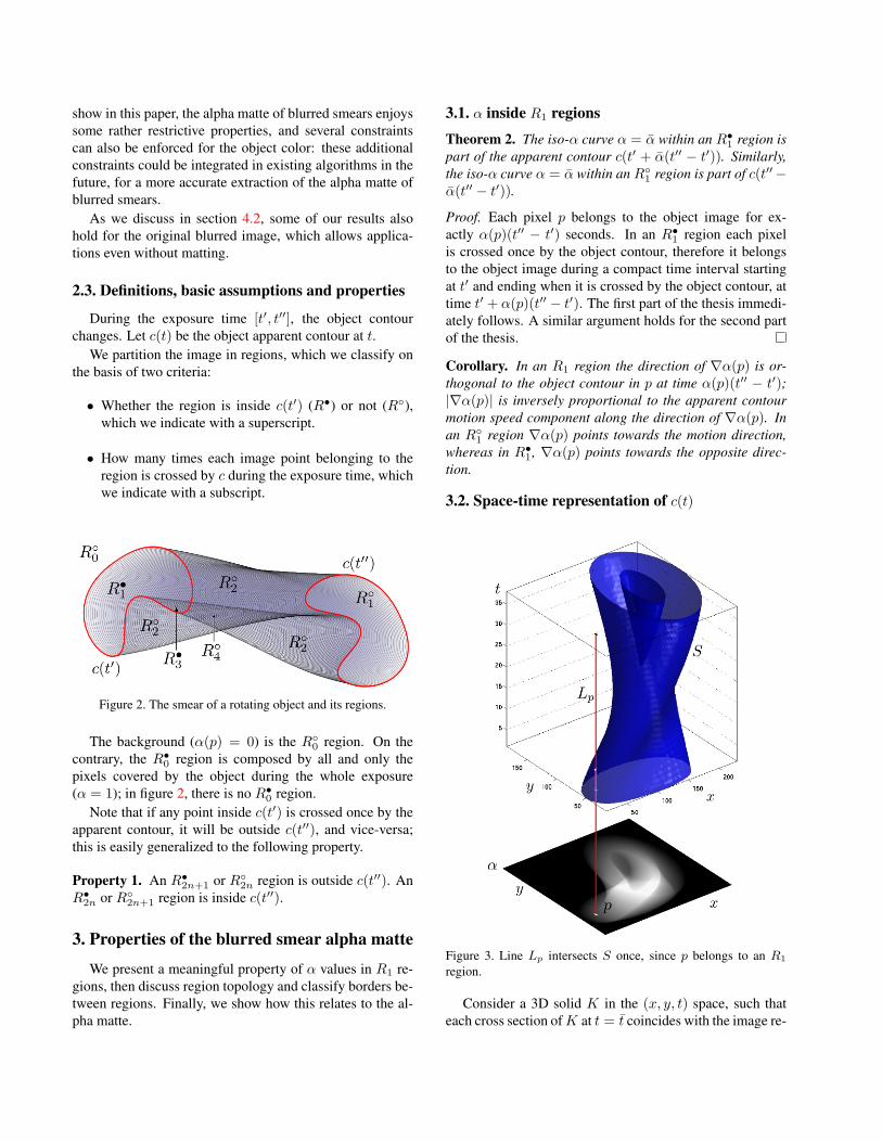
Figure 3. Line Lp intersects S once, since p belongs to an R1

region.

Consider a 3D solid K in the (x, y, t) space, such thateach cross section of K at t = t coincides with the image re-

gion inside c(t). K is bounded by t = t′ and t = t′′ planes,and summarizes the evolution of the object contours duringthe exposure1. We also refer to S (see figure 3), which is thelateral surface of K, i.e. the surface of K except the upper(t = t′) and lower (t = t′′) caps2; the intersection of S witha t = t plane is c(t).

Consider a point p = (px, py) on the x, y plane, and aline Lp in the x, y, t space, defined as x = px, y = py .The number of intersections of S with Lp coincides withthe number of times image point p is crossed by c duringthe exposure time.

Definition 3. An image point p is a degenerate point if andonly if none of the following conditions hold:

(1) Lp is not tangent to S, and p does not belong to eitherc(t′) or c(t′′).

(2) Lp is tangent to S at a single point, and p does notbelong to either c(t′) or c(t′′).

(3) Lp is not tangent to S, and p belongs to c(t′) but not toc(t′′).

(4) Lp is not tangent to S, and p belongs to c(t′′) but notto c(t′).

The physical meaning of said degeneracy is described inthe remarks to the following theorem.

3.3. Borders between regions

Definition 4. We classify borders between regions as fol-lows:

type 1a: connects an Rn region with an Rn+1 region, in-verting the superscript;

type 1b: connects an Rn region with an Rn+1 region, pre-serving the superscript;

type 2: connects an Rn region with an Rn+2 region, al-ways preserving the superscript.

Theorem 5. If apparent contours move with finite speedand a discrete set of degenerate image points exists:

i All possible borders between regions can be classifiedaccording to definition 4; multiple borders may over-lap at a degenerate point.

ii The union set of all type 1a borders coincides withc(t′); the union set of all type 1b borders coincideswith c(t′′).

1A similar representation has been previously proposed for action clas-sification in [22]

2S can be composed by several isolated parts (as in the figure), but weassume that each is smooth everywhere except possibly in a 0-measure set(ridge)

iii A type 2 border is the envelope3 of c(t)|t∈[t1,t2]⊆[t′,t′′];

Proof. Consider a non-degenerate image point. Then, onlyone of the conditions in definition 3 holds.

• If condition (1) holds, then p is not part of a regionborder. In fact, all points p′ in p’s neighborhood be-long to the same region as p, because their Lp′ linesin x, y, t space are crossed by S the same number oftimes; points p′ they are all either inside or outsidec(t′) – thus the region superscript is kept.

• If condition (2) holds, p belongs to a type 2 border. Infact, in p’s neighborhood two points p′ and p′′ existsuch that Lp′ crosses S k times, and Lp′′ crosses Sk + 2 times. The region superscript is kept because allpoints in the neighborhood are either inside or outsidec(t′).

• If condition (3) holds, p belongs to a type 1a border.In fact, in p’s neighborhood two points p′ and p′′ existsuch that Lp′ crosses S k times, and Lp′′ crosses Sk + 1 times. p′ and p′′ are at opposite sides of c(t′),thus the region superscript is inverted.

• If condition (4) holds, p belongs to a type 1b border. p′

and p′′ are not at opposite sides of c(t′), thus the regionsuperscript is preserved.

Remark. Degenerate points are points belonging to morethan a single border; by assuming a discrete set of degen-erate points, we exclude that two borders coincide along afinite curve. In practice, this condition is nearly always met.Examples of violating scenes are an object moving with atrajectory which exactly retraces itself, or an object with astraight horizontal contour part translating horizontally (asegment of a type 1a border overlaps a part of a type 2 bor-der). However, even in scenes not meeting the constraints,

3.4. Interpretation of features on the alpha matte

Features on the alpha matte can be related to region bor-ders by means of the following theorem.

Theorem 6. Under the same broad assumptions as theo-rem 5, and additionally excluding the following degeneratecases:

• presence of cusps on S;

• presence of a ridge on S whose projection on the x, yplane overlaps along a finite curve with a region bor-der or with the projection of a different ridge;

3If c(t) is not smooth, (part of) a type 2 border may represent the locusof points touched by a corner traslating along a direction not included bythe corner itself. This slightly broadens the definition of envelope.

let ∇α be the gradient of α; if p belongs to a single regionborder then ∇α is discontinous in p.

Proof sketch. The theorem can be proven exploiting thespace-time representation of c(t) introduced in section 3.2.α(p) can be interpreted as the total length of P ’s intersec-tion with K. When p crosses a border of type 1, Lp crossesa ridge on the surface of K, which reflects to a disconti-nuity in ∇α: our hypoteses exclude that the discontinuitymay be cancelled by another ridge in K. When p crosses aborder of type 2, P is tangent to K’s surface, which reflectsto a discontinuity in ∇α as well, unless S has a cusp in thetangency point, which is excluded by our hypoteses.

Remark. In practice, the degenerate cases in the theoremstatement almost never occur; they exclude that a discon-tinuity in ∇α is neutralized by a corresponding oppositesource of discontinuity.

The reverse of theorem 6 also holds under the followingmuch more restrictive assumptions, which are met by theperspective image of a strictly convex smooth solid in freemotion:

1. smooth, strictly convex apparent contours;

2. apparent contours moving with continuity in speed.

Then, ∇α has a jump discontinuity always and only acrossa region border. In particular, at a type 1 border we have ajump discontinuity of ∇α in which both the left and rightlimits have finite norm. At a type 2 border, one of the leftor right limits of ∇α has infinite norm.

From the proof of theorem 6 we easily derive that alsoany abrupt change in the speed or orientation of (a part of)apparent contour results in a discontinuity in ∇α. This oc-curs:

• when the object suddenly changes its motion at a timet, e.g. as the result of an impact; in this case a discon-tinuity in ∇α overlapping with c(t) is originated.

• when the moving object is not strictly convex: then adiscontinuity in ∇α at point p occurs as p’s viewingray is bitangent to the object at a given t ∈ [t′, t′′].

• along the path of a corner on the apparent contour.

4. Discussion and practical considerations4.1. Classifying borders and regions

Theorem 6 allows to locate a superset of all region bor-ders by looking for discontinuities in ∇α. Type 2 borders,when representing the envelope of smooth contours, areeasily classified because ∇α has an extremely large normjust besides the border. If the restrictive assumptions hold,which ensure the validity of the reverse of theorem 6, then

there is a one-to-one relation between discontinuities andborders. Else, some discontinuities may be spurious, ande.g. may represent the path of corners in the apparent con-tour which do not originate a legitimate region border, oroutline the contour when the object abruptly changes itsspeed.

R◦0 and R•

0 regions can be initialized where α = 0 andα = 1, respectively.

The type 1 borders constitute the union of c(t′) andc(t′′). Assuming that the two can be separated, there isan uneliminable ambiguity about which is which, so oneis arbitrarily chosen as c(t′) and classified as Type 1a; allcontained regions are set as R•; all remaining regions areR◦. As a result of such uneliminable ambiguity, two con-sistent region labelings are always possible, correspondingto opposite motion directions of the object; one can be trans-formed into the other by simply inverting the superscript ofodd regions.

The region subscripts are not affected by the ambiguity,and can be derived by means of the constraints stated bytheorem 5; we verified on synthetic images that in most im-ages only one consistent labeling (plus its “inverted” twin)satisfies all such constraints.

4.2. Operating on the original image

Under broad assumptions, discontinuities in ∇α resultin discontinuities in the gradient of the original image. Lo-cating region borders and other features directly from theimage gradient is therefore theoretically possible. Practicalfeasibility may be hindered by the possible interference ofthe background and object shading and texture, and greatlydepends on the application scenario.

Figure 4 and Figure 8 illustrate examples of this possi-bility on real images.

4.3. Applications

By locating and classifying regions, their borders, andother discontinuities of∇α, strong constraints on the objectapparent contours during the exposure can be reconstructed.This allows to extract a wealth of motion information fromthe object smear, which would not be available in a sharpimage.

Independent of the specific application scenario, theo-rem 2 allows to partially reconstruct apparent contours atintermediate time instants belonging to the exposure pe-riod, as the union set of an iso-α curve with value α withinR•

1 and an iso-α curve with value 1 − α within R◦1. This

can also be applied for temporal superresolution of apparentcontours in a video whose frames are exposed for a signifi-cant part of the inter-frame interval; this has analogies withShechtman and Caspi’s work [18], which tackles a simi-lar problem with a completely different approach. Another

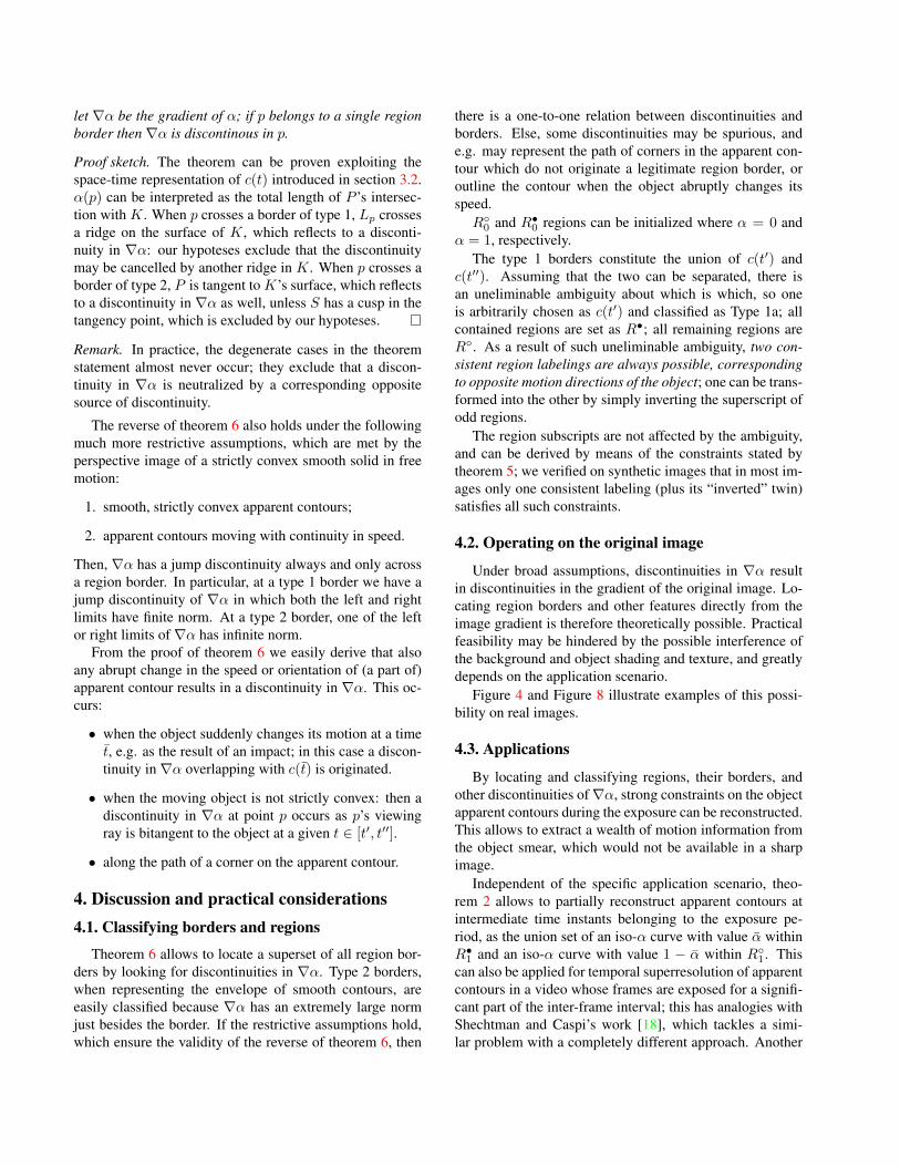
Figure 5. Results on synthetic images. First row: rototraslating torus; from left to right: α; |∇α|; discontinuity in ∇α (see text); groundtruth region subscripts, 0 (black) to 5 (white). Second row: traslating cube; rightmost image represents part of c(t) at intermediate,equispaced instants during the exposure, reconstructed as iso-alpha curves (theorem 2).

Figure 6. Results on real images. First row: white rectangular business card moving on a dark desk; from left to right: the object; theblurred image (from which α follows immediately); |∇α|; discontinuity in ∇α; contour motion as iso-alpha curves. Second row: A planarobject with curvy contours moving on a dark desk. Third row: A candy. Second image is the actual blurred image (exposure time 20 ms):note severe shading and noise. Alpha (third image) is computed using Levin’s matting algorithm.

sophisticated application of the same principle can theoret-ically allow partial 3D reconstruction of a rototraslating ob-ject from a single image ([6]).

Theorem 5 allows to identify c(t′) and c(t′′), which is avaluable information in many practical applications; in fig-ure 8, we exploit this in order to reconstruct the 3D positionand velocity of a moving ball from a single slightly blurredperspective image.

Information about contour envelopes and corner pathscan also be valuable for reconstructing motion in simplescenes, which has applications in machine vision or for un-derstanding high-speed dynamic events with the high reso-lution and low price of an ordinary digital camera.

5. Experimental Results

The theoretical results we presented in the previous sec-tions have been validated by experimental results both onreal (Figures 6 and 8) and synthetic (Figure 5) images, inwhich ground truth is known.

Synthetic images are generated using the popularBlender raytracing software, by creating an animation withseveral hundred frames and averaging all together to obtainthe actual motion-blurred image. Knowledge of the sin-gle frames also allows to automatically compute the groundtruth for the region labeling, as in top right of figure 5. Weextracted alpha data by means of the technique in [7], andverified that the result exactly matches the true alpha, gen-

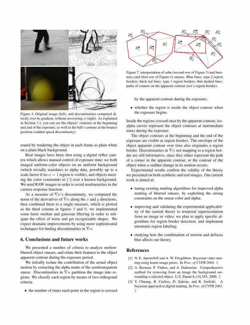
Figure 4. Original image (left), and discontinuities computed di-rectly over its gradient, without recovering α (right). As explainedin Section 3.4, you can see the objects’ contours at the beginningand end of the exposure, as well as the ball’s contour at the bounceposition (sudden speed discontinuity).

erated by rendering the object in each frame as plain whiteon a plain black background.

Real images have been shot using a digital reflex cam-era which allows manual control of exposure time; we bothimaged uniform-color objects on an uniform background(which trivially translates to alpha data, possibly up to ascale factor if no α = 1 region is visible), and objects meet-ing the color constraints in [7] over a known background.We used RAW images in order to avoid nonlinearities in thecamera response function.

As a measure of ∇α’s discontinuity, we computed thenorm of the derivatives of ∇α along the x and y directions,then combined them to a single measure, which is plottedas the third column in figures 5 and 6; we implementedsome basic median and gaussian filtering in order to mit-igate the effect of noise and get recognizable shapes. Weexpect dramatic improvements by using more sophisticatedtechniques for finding discontinuities in ∇α.

6. Conclusions and future worksWe presented a number of criteria to analyze motion-

blurred object smears, and relate their features to the objectapparent contour during the exposure period.

We initially isolate the contribution of the actual objectmotion by extracting the alpha matte of the semitransparentsmear. Discontinuities in ∇α partition the image into re-gions. We classify each region by means of two orthogonalcriteria:

• the number of times each point in the region is crossed

Figure 7. interpretation of cube (second row of Figure 5) and busi-ness card (first row of Figure 6) smears. Blue lines: type 2 regionborders; thick red lines: type 1 region borders; thin dashed lines:paths of corners on the apparent contour (not a region border).

by the apparent contour during the exposure;

• whether the region is inside the object contour whenthe exposure begins.

Inside the regions crossed once by the apparent contour, iso-alpha curves represent the object contours at intermediatetimes during the exposure.

The object contours at the beginning and the end of theexposure are visible as region borders. The envelope of theobject apparent contour over time also originates a regionborder. Discontinuities in ∇α not mapping to a region bor-der are still informative, since they either represent the pathof a corner in the apparent contour, or the contour of theobject when a sudden change in its motion occurs.

Experimental results confirm the validity of the theorywe presented on both synthetic and real images. Our currentwork is aimed at:

• tuning existing matting algorithms for improved alphamatting of blurred smears, by exploiting the strongconstraints on the smear color and alpha;

• improving and validating the experimental applicabil-ity of the current theory to temporal superresolutionfrom an image or video; we plan to apply specific al-gorithms for region border detection, and implementautomatic region labeling;

• studying how the combination of motion and defocusblur affects our theory.

References[1] N. E. Apostoloff and A. W. Fitzgibbon. Bayesian video mat-

ting using learnt image priors. In Proc. of CVPR 2004. 2[2] A. Berman, P. Vlahos, and A. Dadourian. Comprehensive

method for removing from an image the background sur-rounding a selected object. U.S. Patent 6,134,345, 2000. 2

[3] Y. Chuang, B. Curless, D. Salesin, and R. Szeliski. Abayesian approach to digital matting. In Proc. of CVPR 2001.2

Figure 8. An application of our theory to 3D localization of a moving ball from a single perspective image. If the ball appears even slightlyblurred, the traditional method of fitting an ellipse to its apparent contour does not work. We exploit theorem 6, and look for angular pointsalong rectilinear intensity profiles parallel to the ball’s motion; these points lie on c(t′) and c(t′′); by fitting two ellipses on the two sets ofpoints, we are able to reconstruct the 3D position and velocity of the moving ball from a single image. Top row shows a synthetic example(with added gaussian noise): blue dots are discontinuities in the image intensity derivative along profiles, after denoising; red ellipses arethe ground truth for c(t′) and c(t′′); blue ellipses are our estimate, obtained by fitting to blue dots; on the right, each 3D blue line representsour reconstructed position and velocity with a different realization of noise; red line is ground truth; other orientations of the same plot arealso given. Bottom row shows the same algorithm on four different camera images (where ground truth is not available).

[4] P. Favaro and S. Soatto. A variational approach to scene re-construction and image segmentation from motion-blur cues.In Proc. of CVPR 2004. 1

[5] R. Fergus, B. Singh, A. Hertzmann, S. T. Roweis, and W. T.Freeman. Removing camera shake from a single photograph.In ACM SIGGRAPH 2006 Papers. 1

[6] Y. Furukawa, A. Sethi, J. Ponce, and D. Kriegman. Ro-bust structure and motion from outlines of smooth curvedsurfaces. IEEE Trans. on PAMI, 28(2):302–315, 2006. 6

[7] A. Giusti and V. Caglioti. Isolating motion and color in amotion blurred image. In Proc. of BMVC 2007. 2, 6, 7

[8] J. Jia. Single image motion deblurring using transparency.In Proc. of CVPR 2007. 1

[9] S. Kang, Y. Choung, and J. Paik. Segmentation-based imagerestoration for multiple moving objects with different mo-tions. In Proc. of International Conference on Image Pro-cessing (ICIP) 1999. 1

[10] G. Klein and T. Drummond. A single-frame visual gyro-scope. In Proc. of BMVC 2005. 1

[11] A. Levin, D. Lischinski, and Y. Weiss. A closed form solu-tion to natural image matting. In Proc. of CVPR 2006. 2

[12] H.-Y. Lin. Vehicle speed detection and identification from asingle motion blurred image. In Proc. of IEEE Workshop onApplications of Computer Vision, pages 461–467, 2005. 1

[13] H.-Y. Lin and C.-H. Chang. Depth recovery from motionblurred images. In Proc. of International Conference on Pat-tern Recognition (ICPR) 2006, volume 1, pages 135–138. 1

[14] H.-Y. Lin and C.-H. Chang. Automatic speed measurementsof spherical objects using an off-the-shelf digital camera. InProc. of IEEE International Conference on Mechatronics,pages 66–71, 2005. 1

[15] Y. Mishima. Soft edge chroma-key generation based uponhexoctahedral color space. U.S. Patent 5,355,174, 1993. 2

[16] T. Porter and T. Duff. Compositing digital images. ComputerGraphics, 1984. 2

[17] M. Ruzon and C. Tomasi. Alpha estimation in natural im-ages. In Proc. of CVPR 2000. 2

[18] E. Shechtman and Y. Caspi. Space-time super-resolution.IEEE Trans. on PAMI, 27(4):531–545, 2005. Member-Michal Irani. 5

[19] D. Slepian. Restoration of photographs blurred by imagemotion. Bell System Tech., 46(10):2353–2362, December1967. 1

[20] A. R. Smith and J. F. Blinn. Blue screen matting. In SIG-GRAPH ’96: Proc. of the 23rd annual conference on Com-puter graphics and interactive techniques, pages 259–268.2

[21] J. Sun, J. Jia, C.-K. Tang, and H.-Y. Shum. Poisson matting.In ACM SIGGRAPH 2004 Papers, pages 315–321. 2

[22] A. Yilmaz and M. Shah. Actions sketch: A novel actionrepresentation. In Proc. of CVPR 2005. 4