on the automated design of technical systems -...
TRANSCRIPT

On the Automated Designof Technical Systems
From theDepartment of Mathematics and Computer Science
of the University of Paderborn, Germany
The Submitted Dissertation ofAndré Schulz
In Order to Obtain the Academic Degree ofDr. rer. nat.

Advisor: Prof. Dr. Hans Kleine BüningReading Committee: Prof. Dr. Gregor EngelsDate of Oral Examination: November 19th, 2001

Acknowledgments
This thesis is a result of my work in the Knowledge-based SystemsGroup, Department of Methematics and Computer Science, Universityof Paderborn.
I wish to thank my thesis advisor, Professor Dr. Kleine Büning, forhis support of my work, as well as Professor Dr. Engels for evaluatingthis thesis.
I also wish to thank all my colleagues for the valuable discussions,hints and corrections throughout my work on this thesis. I owe specialthanks to Dr. Benno Stein for numerous discussions and for his rigor-ous guidance from which my work benefitted a great deal, and to Dr.Theo Lettmann for his technical and moral support.
Finally, I wish to thank my family and friends for the encourage-ment and support.
André Schulz

4

Contents
1 Introduction 1
1.1 Thesis Structure . . . . . . . . . . . . . . . . . . . . . . . . 4
1.2 Design Support . . . . . . . . . . . . . . . . . . . . . . . . 5
1.3 Model Simplification . . . . . . . . . . . . . . . . . . . . . 7
2 A Design Task 13
2.1 Caramel Syrup Example—Structure . . . . . . . . . . . . 16
2.2 Caramel Syrup Example—Behavior . . . . . . . . . . . . 18
3 Graph Grammar Model for Design 21
3.1 Design Tasks and Graph Transformation Rules . . . . . . 21
3.2 Context-free Design Graph Grammar . . . . . . . . . . . 28
3.3 Context-sensitive Design Graph Grammar . . . . . . . . . 32
3.4 On the Semantics of Labels . . . . . . . . . . . . . . . . . . 35
3.4.1 Terminal and Nonterminal Labels . . . . . . . . . 35
3.4.2 Variable Labels . . . . . . . . . . . . . . . . . . . . 36
3.4.3 Ambiguities . . . . . . . . . . . . . . . . . . . . . . 37
4 Analyzing Systems 39
4.1 Structure Analysis by Graph Grammars . . . . . . . . . . 40
i

Contents
4.2 Caramel Syrup Example . . . . . . . . . . . . . . . . . . . 43
4.3 Behavior Analysis by Simulation . . . . . . . . . . . . . . 45
4.3.1 Classical Simulation . . . . . . . . . . . . . . . . . 47
4.3.2 Qualitative Simulation . . . . . . . . . . . . . . . . 48
4.3.3 Complexity of Design Evaluation . . . . . . . . . . 49
5 Synthesizing Systems 51
5.1 Structure Synthesis by Graph Grammars . . . . . . . . . 52
5.2 Caramel Syrup Example Reviewed . . . . . . . . . . . . . 53
5.3 Graph Topology Restrictions . . . . . . . . . . . . . . . . 55
5.4 Search Techniques . . . . . . . . . . . . . . . . . . . . . . . 56
5.4.1 Label Ordering . . . . . . . . . . . . . . . . . . . . 57
5.4.2 Reinforcement Learning . . . . . . . . . . . . . . . 59
5.4.3 Model Compilation . . . . . . . . . . . . . . . . . . 60
6 Design Language 63
6.1 Requirements . . . . . . . . . . . . . . . . . . . . . . . . . 64
6.1.1 Modification Types . . . . . . . . . . . . . . . . . . 64
6.1.2 Modification Location . . . . . . . . . . . . . . . . 65
6.2 Semantics of Graphical Representation . . . . . . . . . . . 66
6.3 Caramel Syrup Example Reviewed Again . . . . . . . . . 68
7 Classes, Complexity and Design Evaluation 73
7.1 Classical and Design Graph Grammars . . . . . . . . . . 74
7.1.1 The Connecting Approach . . . . . . . . . . . . . . 75
7.1.2 The Gluing Approach . . . . . . . . . . . . . . . . 78
ii

Contents
7.1.3 Hybrid Approaches . . . . . . . . . . . . . . . . . 79
7.1.4 Design Graph Grammars . . . . . . . . . . . . . . 82
7.2 Relationship to PGRS . . . . . . . . . . . . . . . . . . . . . 84
7.3 The Problem of Matching . . . . . . . . . . . . . . . . . . 86
7.3.1 Context and Its Consequences . . . . . . . . . . . 87
7.3.2 The Subgraph Matching Problem . . . . . . . . . . 88
7.3.3 Context within Backward Execution . . . . . . . . 89
7.4 Foundations of Derivations and Membership . . . . . . . 90
7.4.1 Basic Properties . . . . . . . . . . . . . . . . . . . . 90
7.4.2 Special Restrictions . . . . . . . . . . . . . . . . . . 92
7.5 Membership and Derivation in Design . . . . . . . . . . . 96
7.5.1 The Membership Problem . . . . . . . . . . . . . . 97
7.5.2 Solving the Membership Problem . . . . . . . . . 100
7.5.3 Shortest Derivation . . . . . . . . . . . . . . . . . . 103
7.5.4 Distance between Graphs . . . . . . . . . . . . . . 107
8 Summary 111
Bibliography 112
A Applications in Design 121
A.1 Structural Synthesis: Chemical Plants . . . . . . . . . . . 122
A.2 Structural Simplification: Hydraulic Plants . . . . . . . . 131
A.3 Structural Synthesis: Hydraulic Plants . . . . . . . . . . . 137
A.4 Model Reformulation: Wave Digital Structures . . . . . . 140
A.5 Model Reformulation: Parallel-Series Graphs . . . . . . . 143
iii

Contents
Index 150
iv

1 Introduction
The design of a technical system is a process usually dealing with anon-trivial number of components and relations; it remains a majorchallenge for present-day designers. Besides, the design process usu-ally consists of a set of different tasks, such as analysis and optimiza-tion: design does not mean configuration alone, as is the general per-ception.
When tackling a design job, it is useful to look at different modelsof a system from the viewpoints of structure and behavior, which, de-pending on the modeling paradigm, are either loosely or tightly con-nected to each other [Stein, 2001]. Modern design tools focus mainlyon the formulation and processing of behavior models. Support forbehavioral aspects of the design process is indeed essential due to thetime-consuming nature of behavior-related tasks; tasks pertaining tostructural models, which require a great deal of creativity, are usuallyefficiently solved by human experts. Figure 1.1 illustrates this idea.
StructureModel
BehaviorModel
TaskExpectedBehavior
ResultingBehavior
Synthesis Parameterization
AnalysisEvaluation
Manual Processing Automatic Processing
Figure 1.1: The design process according to [Gero, 1990] and modifiedby Stein [Stein, 1995], and the tasks that are traditionally solved man-ually and automatically
1

1 Introduction
Although support for the synthesis of structure models may seemquestionable, it is nonetheless an important step of the design process.This thesis focuses on the structural aspects of the design tasks andaims at providing a foundation for a holistic support of the design pro-cess.
The design process is—depending on the modeling paradigm andgranularity—very complex and at this level even simpler tasks re-main toilsome. Thus, we resort to Functional Abstraction, a paradigmwithin the model construction theory developed by Stein in [Stein,2001], in order to make the task tractable. Stein informally introducesthe paradigm of functional abstraction in the following way:
“At first, we construct a poor solution of a design problem,which then must be repaired.”
In particular, functional abstraction comprises four steps: By meansof model simplification, the original task is abstracted. At this simplifiedlevel, a coarse design can be efficiently generated and, subsequently,enriched with behavior by adding behavior model parts to the struc-ture model. This enriched structure model represents a possibly faultydesign; repair mechanisms are required to produce an acceptable de-sign. Figure 1.2 illustrates the concept of functional abstraction.
Sim
plifi
catio
n
BehaviorLevel
FunctionLevel
OriginalTask
AbstractedTask
StructureModel
Behavior Model(coarse) Solution
Figure 1.2: Efficient solution of a design task by means of functionalabstraction [Stein, 2001].
2

The main contribution of this thesis is the automation of the step“abstracted task → structure model”. Given a description of the de-mands implied by the abstracted task, e. g., in the form of inputs andoutputs, and a set of parameterized system building blocks, both theselection and the connection of the necessary building blocks shall bederived. Moreover, the analysis and improvement of structure and be-havior of a given design is also addressed. In order to achieve thesegoals, state-of-the-art search techniques and knowledge acquisitionmethods are adapted and applied.
The essence of our approach is as follows. A technical system isviewed as a graph, the nodes of the graph describe system buildingblocks, the edges of the graph specify the connections between build-ing blocks and enable the exchange of information and energy. Modi-fications of a technical system are defined as node-insertion and node-deletion operations on the graph. We use graph grammars as a propermeans to precisely specify such modifications, say, to encode an engi-neer’s design knowledge on structure. In order to do this effectively, anew graph grammar class—the design graph grammar—was devisedto allow for an efficient processing within technical domains.
For illustrative purposes we will resort to the domain of chem-ical engineering, which is the main area of application of the DFGproject from which this thesis resulted. Note that in this domaincomputer-based design support is provided in the form of dedicatedconfiguration systems for particular devices such as mixers and ag-itators [Brinkop and Laudwein, 1993, Knoch and Bottlinger, 1993] orspecial heat transfer devices [Götte, 1995, Götte and Schmidt-Traub,1996]. Moreover, there are tools concentrating around simulation, andyet other design tools were developed as tailored CAD programs[Räumschüssel et al., 1993, Marquardt, 1992, Stephanopoulos et al.,1990, Piela et al., 1991, Pantelides, 1988].
In order to validate our approach, a design tool implementing thedescribed methodology has been prototypically developed. This tool,named DIMod (for Domain Independent Modeler), can generate struc-ture models complying with the underlying design knowledge basedon the abstracted task specification. The generated structure model is
3

1 Introduction
enriched with behavior model parts and sourced out to a simulator;the simulation results have to be evaluated in order to determine thequality of the solution—this last step, however, has not been integratedyet into DIMod.
1.1 Thesis Structure
This thesis is organized as follows.
Section 1.2 presents a short survey on the state of the art of modernsystems supporting design tasks. Special attention is given to tools forthe domain of chemical engineering.
Section 1.3 deals with model simplification, a requirement for func-tional abstraction, and addresses the major simplifications introducedas well as some issues related to the modeling granularity.
Chapter 2 gives a description of chemical design tasks, which isillustrated by means of a realistic example.
Chapter 3 examines the requirements imposed by design tasks andintroduces the concept of design graph grammars.
Chapter 4 applies the design graph grammar approach to structureanalysis and briefly discusses the simulation of the underlying model.
Chapter 5 applies the design graph grammar approach to structuresynthesis. Furthermore, search techniques for an efficient generationprocess are investigated.
Chapter 6 sheds some light on different design topics: design repairand optimization.
Chapter 7 supplies a theoretical foundation related to the area ofgraph grammars. The relationship between design graph grammarsand the classical approaches is addressed in detail, and special atten-tion is given to design-related issues.
The appendix contains practical examples of design graph gram-mars used within different domains.
4

1.2 Design Support
1.2 Design Support in Chemical Engineering
According to Marquardt [Marquardt, 1992], modern process model-ing tools can be roughly classified into two types: block-oriented (alsocalled modular) and equation-oriented approaches.
Block-oriented approaches correspond to modeling on the flow-sheet level. The user or engineer works with standardized buildingblocks which model the behavior of a process unit-operation or partof it. Chemical plants are designed by choosing building blocks froma library of standard building blocks and by connecting them appro-priately. These approaches require that an expert create the model li-braries and allow the user to use them at the abstract level describedabove. The manipulation of these building blocks is usually suppliedby modeling languages or visual editors.
Equation-oriented approaches allow for the implementation ofmodels and libraries built thereof by means of declarative modelinglanguages or template routines that can be embedded directly intosome procedural programming language, such as Fortran. These ap-proaches do not provide any modeling tools for experts or users,thereby requiring profound knowledge of the domain.
Since the early 1980’s, various projects whose primary goals wereto provide support for process modeling have been engaged. Only afew of these projects were successful, and the development of somesystems has been suspended altogether. The following table, basedmainly on [Marquardt, 1996], lists some of the projects together withtheir features1:
1Empty entries mean that no information about this specific feature is available andshould not be interpreted as lack thereof.
5

1 Introduction
Tool/ Visual Modeling Uses AI Process
Language Class modeler language simul.
Ascend block general XDiva/Veda
equation process X X
Dylan general XDymola block X general XgProms/SpeedUp
equation general X
HPT process XModass process XDesign-Kit/Model.la
process X
Modeller processModex process XModKit X process XOmSim/Omola
block X general X
Profit process XDIMod block X general X X
The alleged features of some systems could not be checked by theauthor due to availability issues. Though some tools may share thesame properties, they often do so to varying degrees. The use of ar-tificial intelligence, for instance, is often limited to the availability ofassistants or wizards, or, in a few cases, to an “intelligent” preprocess-ing of the equation systems.
The approaches presented in this thesis were implemented to a cer-tain extent in DIMod, a process modeling tool prototype developed atthe University of Paderborn; they are described in detail in the chap-ters 4, 5 and 6. The main concern in DIMod is the support for structure-related tasks; process simulation support is restricted to qualitativesimulation or sourced out to third-party simulation tools2.
2At the present development stage only Ascend is supported.
6
1.3 Model Simplification
Although DIMod possesses many features common to moderntools, it outstands in its ability to automatically synthesize and ana-lyze structure models.
1.3 Model Simplification
An automation of the design steps at the original model level wouldbe very expensive—present systems limit automation to human-un-friendly tasks like simulation, and the effort involved there is highenough. However, our goal is to provide support throughout the de-sign procedure, and at this level fine granular processing remains in-surmountable with present-day technology.
Another pressing reason for a modeling depth shift is the targeteddesign support type, namely the automation of structure related tasks.Within this scope information pertaining to the physical properties ofa system does not play a major role.
Instead of deriving a concrete solution at the modeling level im-posed by the supplied demands, the original task is simplified. Onthis abstract level, a solution can be efficiently calculated and trans-ferred back to the physical level, although some adjustments may benecessary at this point (see chapter 6).
The following model simplification steps—named according to[Frantz, 1995]—lead to a more tractable design problem:
• Model boundary simplification. Assumptions pertaining to the ex-ternal features of the model—input variable space, global restric-tions etc.—are made:
– Simple task assumption. It is general practice to combine dif-ferent chemical processes that share some partial chains inorder to save costs. Such a combination corresponds to thesolution of different tasks simultaneously. However, thisprocedure belongs to optimization; therefore, overlappingplant structures are segregated and dealt with separately,
7

1 Introduction
i. e., we solve each task individually. The following figureillustrates this concept.
– Model context. The way models, or parts of models, are em-bedded into a context is clearly defined. Pumps, for exam-ple, have a strict structural relationship; they have one inputand one output, i. e., the degree is fixed, and the predecessorof a pump must be another device.
– Limited input space. Firstly, we concentrate on tasks of thefood processing branch of the chemical engineering do-main. This restriction results in further simplifications: Thechemical plants to be designed do not exceed a certain mag-nitude, as well as the range of some variables, such as tem-perature, which is limited to “small” values, say, below200°C.Furthermore, the focus is laid on liquid mixtures. Thismeans that at least one input has to be a fluid.Another restriction is the number of relevant substanceproperties. During design generation, decisions are takenbased on the abstract values of a small set of substanceproperties, such as temperature, viscosity, density, mass andstate. Properties such as heat capacity, heat conductivity orcritical temperature and pressure are neglected at this point.
8

1.3 Model Simplification
– Approximation. Instead of using different functions and for-mulas that apply under different conditions, only one func-tion or formula covering the widest range of restrictions isused in each case. For example, there are over 50 differ-ent formulas to calculate the viscosity of a mixture, mostof which are very specialized versions and only applica-ble under very rare circumstances—the formula ln(η) =∑i ϕi · ln(ηi), however, is very often applicable and deliv-ers a good approximation, even in the complicated cases.
• Behavioral simplification. Now the focus is shifted to aspectswithin the model, where the behavior of components is simpli-fied:
– Causal decomposition. To prevent components from exertinginfluence on themselves, feedback loops are ruled out. Thissimplification step makes structural manipulation and be-havioral analysis easier.The situation depicted below shows a cycle within a chemi-cal plant. The purpose of the backward edge is to transportevaporated substance back into the mixer; this gaseous sub-stance condenses on the way.
– Numeric representation. Although the use of crisp valuesleads to exact results, fuzzy sets are used to represent essen-tial value ranges. This simplification diminishes the combi-natorial impact on our graph grammar approach, since sub-stance properties are coded into edge labels and the use ofcrisp values would lead to an excessive number of rules.The following figure shows the fuzzy representation of thesubstance property “viscosity”:
9

1 Introduction
500 5000
0.5
1.0
01
low medium high
mPas
– State aggregation. In general, the material being processedwithin a device is not in one state, but actually in variousdifferent ones. For instance, inside a heat transfer device afluid may be, depending on the reading point, cold, warm,in liquid form or gaseous. This behavior is simplified by as-suming that, inside any device, a material will be in one sin-gle state.
– Temporal aggregation. Time is neglected, making any state-ments about continuous changes to material properties nolonger possible; changes to material properties are con-nected to entry and exit points within the plant structure.
– Entity aggregation by function. Different device entities arerepresented by one device performing a function commonto all devices. For example, all different mixer types couldbe described by one special mixer, as shown below.
– Entity aggregation by structure. Devices usually consist of dif-ferent parts that can be configured separately. For instance,a plate heat transfer device is composed of a vessel and avariable number of plates. The arrangement of the plateswithin the vessel is a configuration task.
10

1.3 Model Simplification
The following figure sketches the composition of a plateheat transfer device and of an anchor mixer.
+
+ +
– Function aggregation. In contrast to entity aggregation byfunction, where devices are represented by a special device,we aggregate here functions. For instance, mixers are capa-ble of performing different functions, such as homogeniza-tion, emulsification, aeration, suspension etc.
• Derived relationships. Some fields of chemical engineering still re-main unveiled and are dealt with as black boxes. In such casesone has to resort to look-up tables and interpolation, as far assufficient information is available. For example, the output ofa mixer, measured in terms of the Reynolds and Newton num-bers, has to be determined experimentally, and this data is usu-ally only available as tables.
Remarks. The model simplification steps listed above can be classifiedinto two different types: Steps pertaining to the model structure andsteps belonging to the model behavior. Note that steps may be con-nected to both structure and behavior.
The steps that simplify the model structure—simple task assump-tion, model context, limited input space, causal decomposition, nu-meric representation, entity aggregation by function—yield a modelthat is fitting to be processed with graph grammars. These steps re-strict the graph structure and specify the types and granularity of nodeand edge labels.
The steps belonging to the model behavior—limited input space,approximation, causal decomposition, numeric representation, stateand temporal aggregation, entity aggregation by structure, functionaggregation, derived relationships—result in a model suitable forqualitative simulation, as described in chapter 4.
11
1 Introduction
The model simplification steps performed here relate to the domainof chemical engineering. For other domains not necessarily the samesteps will be appropriate; the modeler has to determine which modelsimplification steps are fitting individually.
12

2 A Design Task from the Domain ofChemical Engineering
The approach presented in this thesis may be suited to tackle variouskinds of design problems in different domains. However, we concen-trate on a particular part of chemical engineering: The design of plantsfor the food processing industry.
A chemical plant can be viewed as a graph, where the nodes rep-resent the devices, or unit-operations, and the edges correspond tothe pipes responsible for the material flow. Typical unit-operationsare mixing (homogenization, emulsification, suspension, aeration etc.),heat transfer, and flow transport. Modifications of a chemical processinclude the insertion of devices, rearrangement of chains, removal orsubstitution of redundant devices etc. At the abstract level these mod-ifications match the graph operations mentioned earlier.
The task of designing a chemical plant is defined, as in many otherfields, by the given input and the desired output. The goal is to mixor transform various input substances in such a way that the result-ing product meets the imposed requirements—in order to achieve thisgoal, a chemical plant, consisting of properly configured devices, hasto be devised. Figure 2.1 illustrates the solution process followed ingeneral practice.
The steps depicted in Figure 2.1 can be described in more detail asfollows:
1. Preliminary examination. This step includes any preparatory mea-sures that must be taken prior to beginning with the design pro-cess. This includes examining the task specification, i.e., the input
13

2 A Design Task
Solution
Task Preliminary examination
Choice of unit-operations
Structure definition
Configuration of components
Optimization
Figure 2.1: Steps in the design process of a chemical plant.
substances and the desired output, from which possibly implicitinformation can be extracted. For instance, the input substancesmay differ in a certain essential property like “solubility in wa-ter”, and, if there are more than two input substances, it mightbe necessary to process the ones belonging to the same solubilitytype before dealing with all input substances together. This canbe done by grouping or clustering the substances according toprespecified properties.
2. Choice of unit-operations. After examining the substances involvedin the desired chemical process, abstract building blocks, so-called unit-operations, are chosen in compliance with certainrules. For example, if the output mixture should have a temper-ature that is substantially different from the temperature of theinput substances, then the unit-operation heat transfer is needed.Moreover, using the example of the last step, if at least two sub-stances have different solubility properties, then the unit-opera-tion emulgation is necessary. Similarly, any other conclusions con-cerning the choice of unit-operations are drawn in a rule-basedfashion.
In practice, engineers choose concrete devices at this stage—theuse of abstract building blocks is done implicitly.
14

3. Structure definition. The previous step produces a set of unit-op-erations devoid of any structure, i.e., the unit-operations are still“unconnected”. To find an apt topology, different circuits aretried until one that meets the requirements is found. This well-known propose-and-revise behavior has been also applied to thefield of chemical engineering [Brinkop and Laudwein, 1993].
Typically, the initially devised topology represents a good solu-tion. However, a first calculation of the resulting mixture andits properties may show that certain constraints, such as max-imum mixing time, cannot be met by the proposed topology.Therefore, the engineer may have to adapt his initial solution byadding or removing certain devices, or the topology itself has tobe changed. This procedure is reiterated until all requirementsare met.
4. Configuration of devices. The chosen devices, still represented byunit-operations, are instantiated. Beginning with the first unit-operation in the process chain, concrete devices are chosen froma database. Since different devices of the same class often pro-duce outputs with slightly different properties, these changesmust be propagated throughout the chain, thus influencing thechoice of later devices.
Alternatively, this step may also be performed before the struc-ture is defined (but no propagation takes place at this point).
5. Optimization. The plant’s functionality is tested whether it meetsthe imposed requirements. If the designed plant fails to fulfillany of these requirements, some changes have to be applied ei-ther to the structure or to the set of chosen devices.
Even if the plant represents a solution to the problem, the engi-neer might still want to refine it to reduce energy consumptionor to decrease mixing time. These optimizations or modificationsalso require some changes to the plant, making the return to aprevious step obligatory.
15

2 A Design Task
2.1 Caramel Syrup Example—Structure
We now present a concrete example for the design process describedin section 2. Here the emphasis is laid on the structure of the design;section 2.2 will address the behavior of the design.
The following task specification excerpt shall help illustrate theusual design procedure performed by an engineer.
Name State Mass Temp. Viscositysugar solid 47.62% 20°C –water liquid 15.75% 20°C 0.0010012 Passtarch syrup liquid 36.63% 20°C 0.2-1.6 Pascaramel syrup liquid 100.00% 110°C ?
The goal is to produce caramel syrup, which is necessary for theproduction of caramel bonbons, using water, starch syrup and sugar.
The following table containing viscosity values of sugar solution,a possible intermediate product, is also available, although it does notbelong to the task specification per se:
Temperature Viscosity (71% solution)0°C 5000 Pas
10°C 1000 Pas20°C 500 Pas30°C 250 Pas40°C 130 Pas50°C 80 Pas60°C 50 Pas70°C 30 Pas80°C 20 Pas
Based on this task specification, the following steps pertaining tothe structure are performed in compliance with the general proceduredepicted in section 2:
16

2.1 Caramel Syrup Example—Structure
1. Preliminary examination. The first observation made by the engi-neer is that one of the substances, sugar, is a solid and must bedissolved within one of the other input liquids. Since water hasa lower viscosity than starch syrup, it will be better to mix sugarand water first and then add the starch syrup to the solution.Depending on the mass ratios the water may have to be heatedbeforehand to increase solubility.
2. Choice of unit-operations. The comparison of the mass ratios ofsugar and water leads to the conclusion that heating is necessary;thus, a heat transfer unit-operation is needed to heat the water.The heated water and the sugar are then mixed—for this purposea mixing unit-operation for lower viscous substances is appro-priate. To avoid recrystallization, the starch syrup should also beheated, thereby making another heat transfer unit-operation nec-essary. Finally, the heated sugar solution and the heated starchsyrup are mixed. In order to reach the required temperature of110°C, another heat transfer unit-operation will be needed. Fur-thermore, pump unit-operations are required to transport thesubstances between devices.
3. Structure definition. The choice of unit-operations, although hav-ing no direct impact on the structure, allows for certain conclu-sions pertaining to the ordering of the unit-operations. In thiscase this ordering is relatively evident; Figure 2.2 shows the cho-sen topology.
Starchsyrup
Water
Sugar
Caramelsyrup
Figure 2.2: The first design of the example process.
17

2 A Design Task
2.2 Caramel Syrup Example—Behavior
The example presented in the previous section shows how an abstractdesign can be generated, using a simplified task description. The re-sult of the generation process is a feasible structure complying with thesimplified demands. This, however, does not represent a complete de-sign, since all devices remain abstract. Thus, this abstract model mustbe enhanced with concrete device data—static and dynamic parame-ters.
The following steps determine the behavior of the design and makesome corrections, if applicable:
4. Configuration of devices. Based on the mass, the volume, and theother properties of the involved substances, matching devicesare chosen from databases or data sheets. For the sake of simplic-ity we will refrain from a detailed description here and refer toFigure 2.3, where the abstract design with additional data fromthe underlying model is shown.
5. Optimization. The computed properties of the plant design usu-ally represent feasible values, but improvement may still be pos-sible. With this goal in mind, the parameterization process is re-peated and parameters adjusted accordingly. In our case the lastheat transfer unit-operation of the process chain represents anoverkill—the last mixing unit-operation is then slightly changedso that only devices with a built-in heat transfer unit are consid-ered. This change shortens the process chain, thereby reducingcosts and mixing time. The final design is depicted by Figure 2.3.
Alternatively, another design with fewer devices is conceivable.For instance, water and starch syrup can be mixed first, and the re-sulting solution used to dissolve sugar. This structure choice wouldrequire one heat transfer unit-operation less than the proposed designbecause both water and the starch syrup have to be heated to the sametemperature, which is best done if both substances are mixed togetherbeforehand. However, this alternative would cause a longer mixing
18

2.2 Caramel Syrup Example—Behavior
Starchsyrup
Water
Sugar
Caramelsyrup
[0-50C]
[0-50C]45l
40l
15kg
[0-0.5 m3/h]
[0-0.5 m3/h]
[0-0.5 m3/h]
20C
20C
70C
70C
70C, ≤0.2Pas
70C, ≤0.001Pas
Propeller75% Solution≈ 60-70C≈ 30Pas
100l≤ 110C≈ 4Pas
PropellerRange: [0-50C]≤ 110C≈ 4Pas
Figure 2.3: Design showing part of the underlying model.
time, since the sugar must be dissolved in a more viscous solution(compared to pure water). Figure 2.4 shows this alternative solution.
Starchsyrup
Water
Sugar
Caramelsyrup
Figure 2.4: Alternative design of the example process.
19

2 A Design Task
20

3 Graph Grammar Model for Design
Each of the steps depicted in Figure 2.1 can be automated in an isolatedfashion. However, a separate processing may lead to loss of informa-tion, since the choice of a unit-operation often affects the structure andvice versa. For example, the choice of a certain mixer might influencethe decision whether a heat transfer device is necessary or not, therebypossibly causing a change to the topology. Likewise, a certain orderingof the devices within the plant structure can make one of them super-fluous.
Due to the intertwined nature of these steps, it is strongly desirableto combine the choice of unit-operations and the structure definition tomake use of all information available. One way of tackling both taskssimultaneously is to use a graph grammar to generate feasible designsin a controlled manner, thus allowing for an incremental execution ofthe mentioned steps. The graph grammar will not only be used for con-trolled generation, but also for analysis tasks, optimization and repairtasks, and also for dynamic visualization purposes.
In the following we analyze the requirements imposed by the var-ious design aspects and introduce suitable graph grammar models tofulfill them. Finally, special issues concerning the semantics of designgraph grammars are addressed.
3.1 Design Tasks and Graph Transformation Rules
A technical system can be described by a labeled graph. The nodes ofthe graph designate the system’s items, the graph’s edges define rela-tions between the items, labels specify the types of nodes and edges.
21

3 Graph Grammar Model for Design
The following definition introduces this concept formally.
Definition 1 (Labeled Graph)
A labeled graph is a tuple G = 〈VG, EG,σG〉 where VG is the set of nodes,EG ⊆ VG × VG is the set of directed edges, and σG is the label function,σG : VG ∪ EG → Σ, where Σ is a set of symbols, called the label alphabet.
Notation: (v1, v2, l) represents a directed edge with tail v1, head v2 and labell. {v1, v2, l} denotes an undirected edge with label l, which can be viewedas two directed edges, (v1, v2, l) and (v2, v1, l). Edges without labels will bewritten as (v1, v2) or {v1, v2}.
The design of a system encompasses a variety of different aspectsor tasks and not only the traditional construction process with whichit is usually associated. For each of these tasks different operations ofvarying complexity are required:
• Insertion and deletion of single items in a system
• Change of specific item and connection types
• Manipulation of sets of items, e. g., for repair or optimization
The operations delineated above can be viewed as transformationson graphs; they are of the form target → replacement. A precise specifi-cation of such “graph transformation rules” can be given with graphgrammars. A central concept in this connection is bound up with thenotions of matching and context, which, in turn, build up on the con-cept of isomorphism (see, for example, [Jungnickel, 1999]). Complexityissues are addressed in chapter 7.
Definition 2 (Isomorphism, Isomorphism with labels)
Let G = 〈VG, EG〉 and H = 〈VH , EH〉 be two graphs. An isomorphismis a bijective mapping ϕ : VG → VH for which holds: {a, b} ∈ EG ⇔{ϕ(a),ϕ(b)} ∈ EH, for any a, b ∈ VG. If such a mapping exists, G and Hare called isomorphic.
22

3.1 Design Tasks and Graph Transformation Rules
G and H are called isomorphic with labels, if G and H are labeled graphswith labeling functions σG and σH, and the following additional conditionholds: σG(a) = σH(ϕ(a)) for each a ∈ VG, and σG(e) = σH(ϕ(e)) for eache ∈ EG, where ϕ(e) = {ϕ(a),ϕ(b)} if e = {a, b}.
Figure 3.1 shows an example of isomorphic and non-isomorphicgraphs.
a
b
c
d
e
ab
c d
e
a
b
c
d
e
G H1 H2
Figure 3.1: A graph G, a graph H1 that is isomorphic to G, and a graphH2 that is not isomorphic to G.
Definition 3 (Matching, Context)
Given are a labeled graph G = 〈V, E,σ〉 and another labeled graph, C.Each subgraph 〈VC , EC,σC〉 in G, which is isomorphic to C, is called a match-ing of C in G. If C consists of a single node only, a matching of C in G is callednode-based, otherwise it is called graph-based.
Moreover, let T be a subgraph of C, and let 〈VT , ET,σT〉 denote a match-ing of T in G. A matching of C in G can stand in one or more of the followingrelations to 〈VT , ET ,σT〉:
1. VT ⊂ VC , VT = ∅. Then the graph 〈VC, EC,σC〉 is called a context ofT in G.
2. 〈VC, EC,σC〉 = 〈VT , ET,σT〉. Then T is called context-free.
A matching of a graph T in G is denoted by T̃. In general, we will notdifferentiate between a graph T and its isomorphic copy.
23

3 Graph Grammar Model for Design
a) b) c)
ab
c d
b
c
Ga
bc
d
TC
ab
c d
b
c
Tab
c d
b
c
Tab
c d
b
c
T
Figure 3.2: Above, a context graph C including a target graph T, anda host graph G. Below: a) strict degree matching of T in G;b) matching of T in G; and c) matching of C in G, but nocontext of T.
Figure 3.2 illustrates the notions of matching and context.
Remarks. A matching T̃ of a graph T within another graph G repre-sents a subgraph of G, which means that potentially every node of T̃may be connected to the remainder of G by arbitrarily many edges.This matching concept may be sufficient for most purposes, but thedomain of technical systems requires more flexibility. Thus, the term“matching” is refined to allow the matching of nodes with a precisenumber of edges. This type of matching is called strict degree matching;in practice, the use of this type of matching will be indicated by anasterisk appended to a node instance, as in T = 〈{1∗, 2}, {(1, 2)}〉.
Existing graph grammar approaches are powerful, but lack withintwo respects. Firstly, the notion of context is not used in a clear andconsistent manner, which is also observed in [Rozenberg, 1997], page97. Secondly, graph grammars have not been applied seriously in or-der to solve synthesis and analysis problems in the area of techni-cal systems—graph grammar solutions focus mainly on meta prob-
24

3.1 Design Tasks and Graph Transformation Rules
lems [Rozenberg, 1997, Ehrig et al., 1999a,b, van Eekelen et al., 1998,Kaul, 1986, 1987, Korff, 1991, Lichtblau, 1991, Rekers and Schürr, 1995,Schürr et al., 1995, Schürr, 1997a].
The systematics of design graph grammars introduced here ad-dresses these shortcomings. Figure 3.3 relates classical graph grammarterminology to typical design tasks; the following list presents exam-ples for the differently powerful rule types. A precise analysis of the re-lationship between classical graph grammar families and design graphgrammars can be found in chapter 7.
Node-based Graph-based
withcontext
context-free
NLC NCE
Insertion,deletion
(synthesis)
Manipulationof types
(synthesis,analysis)
Typed structuralmanipulation
(repair, optimization)
Structuralmanipulation(model trans-
formation)
NCE
withcontext
context-free
NCE withoutedge labels
Target
DesignTasks
ClassicalGraph
Grammars
Figure 3.3: Graph grammar hierachy for the various design tasks. Theabbreviations NLC and NCE denote classical graph gram-mar families.
• Node → node: Context-free transformation based on node la-bels. Graph grammars with rules of this type are called node labelcontrolled graph grammars (NLC grammars). The following fig-ure illustrates a type modification of a mixing unit, which can berealized by this class of rules.
25

3 Graph Grammar Model for Design
• Node → graph: Context-free transformation based on node la-bels (NLC grammars). The following figure shows the replace-ment of an ideal voltage source by a resistive voltage source (syn-thesis without context).
e e
+ +
• Node with context → node: Node-based transformation basedon node labels and edge labels. Graph grammars with rules ofthis type are called neighborhood controlled embedding graph gram-mars (NCE grammars). The clustering of graphs (analysis andsynthesis with context) is an example for this type of transfor-mation and is depicted in the following figure.
A B
C
• Node with context → graph: Node-based transformation basedon node labels and edge labels (NCE grammars). The follow-ing figure shows the replacement of an unknown unit by insert-ing heat transfer and pump units to fulfill the temperature con-straints (synthesis with context):
TlowThigh Tlow
Thigh?
The following figure illustrates the replacement of an unknownunit by inserting a heat transfer unit, a pump unit and a mixingunit (synthesis with context):
26

3.1 Design Tasks and Graph Transformation Rules
Tlow Thigh Thigh
ThighThigh
Tlow?
• Graph → graph: Context-free transformation based on graphswithout edge labels (NCE grammars without edge labels). Thereplacement of two resistors in series by one resistor, an examplefor structural manipulation, is depicted below.
Another example for transformation of this type is given by theconversion of a structure description tree into a parallel-seriesgraph (model transformation):
S
P
S
∆ ∆ ∆ ∆ ∆
∆∆
∆
∆∆
• Graph with context → graph: Context-sensitive transformationbased on graphs with edge labels (NCE grammars). The follow-ing figure shows the insertion of a bypass throttle (repair, opti-mization), which represents such a transformation.
27

3 Graph Grammar Model for Design
3.2 Context-free Design Graph Grammar
What happens during a graph transformation is that a node, t—or asubgraph, T—in the original graph G is replaced by a graph R. Putanother way, R is embedded into G.
In the following we will provide a formal basis for the illustratedgraph transformations.
Definition 4 (Host Graph, Context Graph, Target Graph, ReplacementGraph, Cut Node)
Within the graph transformation context a graph can play one of the fol-lowing roles:
• Host graph G. A host graph represents the structure on which thegraph transformations are to be performed.
• Context graph C. A context graph represents a matching to be foundin a host graph G. The graph C is part of the left-hand side of graphtransformation rules.
• Target graph T. A target graph represents a graph whose matching ina host graph G is to be replaced. If T is a subgraph of a context graph C,then the occurrence of T within the matching of C in G is to be replaced.The graph T is part of the left-hand side of graph transformation rules.In case T consists of a single node, it is called target node and denotedby t.
• Replacement graph R. A replacement graph represents a graph ofwhich an isomorphic copy is used to replace a matching of the targetgraph T in the host graph. The graph R is part of the right-hand side ofgraph transformation rules.
• The nodes of the host graph that are connected to the matching of T arecalled cut nodes.
Informally, a graph grammar is a collection of graph transforma-tion rules, each of which is equipped with a set of embedding instruc-
28

3.2 Context-free Design Graph Grammar
tions. The following definition provides the necessary syntax and se-mantics.
Definition 5 (Context-free Design Graph Grammar)
A context-free design graph grammar is a tuple G = 〈Σ, P, s〉 with
• Σ is the label alphabet used for nodes and edges1,
• P is the finite set of graph transformation rules,
• and s is the initial symbol.
The productions of the set P are graph transformation rules of the formT → 〈R, I〉 and with the following semantics: Firstly, a matching of thetarget graph T is searched within the host graph G. Secondly, this occurrenceof T along with all incident edges is deleted. Thirdly, an isomorphic copy ofR is connected to the host graph according to the semantics of the embeddinginstructions.
• T = 〈VT, ET ,σT〉 is the target graph to be replaced,
• R = 〈VR, ER,σR〉 is the possibly empty replacement graph.
• I is the set of embedding instructions consisting of tuples of the form((h, t, e), (h, r, f )), where
– h ∈ Σ is a label of a node v ∈ G \ T,
– t ∈ Σ is a label of a node w ∈ VT,
– e ∈ Σ is the label of the edge {v, w},
– f ∈ Σ is another edge label not necessarily unequal to e, and
– r ∈ VR is a node in R.1Labels are used to specify types and as variables for other labels. To avoid confusion,
variable labels will be denoted by capital letters, and all other labels with small let-ters.
29

3 Graph Grammar Model for Design
An embedding instruction ((h, t, e), (h, r, f )) is interpreted as follows:If there is an edge with label e connecting a node labeled h with thetarget node t, then the embedding process will create a new edge withlabel f connecting the node labeled h with node r. See section 3.4 for adetailed discussion about the semantics of embeddings instructions.
The execution of a graph transformation rule p on a host graph G yieldinga new graph G′ is called a derivation step and denoted by G ⇒p G′. Asequence of such derivation steps is called derivation.
Remarks. In many cases we will not need the complete expres-sive power of the embedding instruction definition. If the targetgraph consists of a single node and edge labels are left unchanged2,then an embedding instruction may be written as (e, r) instead of((h, t, e), (h, r, e)).
Example. In order to illustrate how a graph transformation rule works,let us view the transformation of a graph G into a graph G′, as depictedin Figure 3.4.
G’G
a
b c
d e
f g f
Tn
a d e
f f
R
Figure 3.4: Application of a context-free graph transformation rule ona host graph G showing a target graph T and a replacementgraph R.
A graph transformation rule T → 〈R, I〉 that performs the transfor-mation shown in Figure 3.4 has the following components:
2 In the literature grammars that do not change edge labels in the embedding processare called neighborhood uniform grammars.
30

3.2 Context-free Design Graph Grammar
• Target T = 〈VT, ET ,σT〉 = 〈{1, 2}, {{1, 2}}, {(1, b), (2, c)}〉• Replacement R = 〈VR, ER,σR〉 = 〈{3}, {}, {(3, n)}〉• Set I of embedding instructions with I = {((a, b, f ), (a, n, f )),
((e, c, f ), (e, n, f ))}. Alternatively, one can employ variable la-bels, which yields I = {((X, Y, f ), (X, n, f ))}.
In the following we present the formal representation of a simpledesign graph grammar.
Example. Let G = 〈Σ, P, s〉 be a design graph grammar that comprisessome transformations described in section 3.1.
• Σ = {?, A, B, C, D, low, high, pump, heater, mixer},
• P = {r1, r2},
• s = ?
Rule r1 is defined as follows:
T = 〈{1, 2, 3}, {(1, 2), (2, 3)}, {(1, A), (2, ?), (3, B),((1, 2), low), ((2, 3), high)}〉
R = 〈{4, 5, 6, 7}, {(4, 5), (5, 6), (6, 7)},{(4, A), (5, pump), (6, heater), (7, B),((4, 5), low), ((6, 7), high)}〉
I = {((D, A, E), (D, A, E)), ((D, B, E), (D, B, E))}
The graphical representation of the above rule is:
TlowThigh Tlow
Thigh?
31

3 Graph Grammar Model for Design
The formal representation of rule r2 is:
T = 〈{1, 2, 3, 4}, {(1, 3), (2, 3), (3, 4)}, {(1, A), (2, B),(3, ?), (4, C), ((1, 3), low), ((2, 3), high), ((3, 4), high)}〉
R = 〈{5, 6, 7, 8, 9, 10}, {(5, 7), (7, 8), (8, 9), (6, 9), (9, 10)},{(5, A), (6, B), (7, heater), (8, pump), (9, mixer), (10, C),((5, 7), low), ((6, 9), high), ((9, 10), high)}〉
I = {((D, A, E), (D, A, E)), ((D, B, E), (D, B, E)),((D, C, E), (D, C, E))}
The formal described above corresponds to the following graphicalnotation:
Tlow Thigh Thigh
ThighThigh
Tlow?
3.3 Context-sensitive Design Graph Grammar
In section 3.2 the notion of context-free design graph grammars was in-troduced. However, it is conceivable that context-sensitive rules maybe necessary, which fact makes context-free graph grammars inad-equate. In the literature, the natural extension of context-free graphgrammars is called context-sensitive graph grammars. The following def-inition is based on definition 5 of section 3.2.
Definition 6 (Context-sensitive Design Graph Grammar)
A context-sensitive design graph grammar is a tuple G = 〈Σ, P, s〉 asdescribed in definition 5, but where the productions of the set P are graphtransformation rules of the form 〈T, C〉 → 〈R, I〉 with
• T = 〈VT , ET ,σT〉 is the target graph to be replaced,
32

3.3 Context-sensitive Design Graph Grammar
• C is a supergraph of T, called the context,
• R = 〈VR, ER,σR〉 is the possibly empty replacement graph.
• I is the set of embedding instructions.
The semantics of a graph transformation rule 〈T, C〉 → 〈R, I〉 is asfollows: Firstly, a matching of the context C is searched within the hostgraph. Secondly, an occurrence of T within the matching of C alongwith all incident edges is deleted. Thirdly, an isomorphic copy of R isconnected to the host graph according to the semantics of the embeddinginstructions.
The set I of embedding instructions consists of tuples of the form((h, t, e), (h, r, f )), which are interpreted as in the context-free case.
In the following we will not always distinguish between bothgraph grammar types, since this should be obvious from the contextand rule types.
Example. In order to illustrate how a context-sensitive graph transfor-mation rule works, let us view the transformation of a graph G into agraph G′, as depicted in Figure 3.5.
G
a
bc
d
T
C
f
g
a
n
d
R
C
f
g
G’
Figure 3.5: A context-sensitive graph transformation rule showing ahost graph G, a target graph T, a context graph C and areplacement graph R.
33

3 Graph Grammar Model for Design
A graph transformation rule 〈T, C〉 → 〈R, I〉 that performs thetransformation shown in Figure 3.5 has the following components:
T = 〈VT , ET,σT〉 = 〈{1, 2}, {{1, 2}}, {(1, b), (2, c)}〉C = 〈VC, EC,σC〉〈{3, 4, 5, 6, 7, 8}, {{3, 4}, {3, 7},
{7, 8}, {4, 8}, {3, 5}, {5, 6}, {6, 8}},{(3, a), (5, b), (6, c), (8, d), ({3, 5}, f ), ({6, 8}, g)}〉
R = 〈VR, ER,σR〉 = 〈{9}, {}, {(9, n)}〉I = {((a, b, f ), (a, n, f )), ((d, c, g), (d, n, g))}
Remarks. Design graph grammars differ not only in matters of context,but also as far as the size of the target graph of the graph transforma-tion rules is concerned. If all target graphs of the graph transformationrules consist of single nodes, then the graph grammar is called node-based, otherwise it is called graph-based. This distinction is of relevance,since node-based and graph-based graph grammars fall into differentcomplexity classes due to the subgraph matching problem (see 7.3.2)connected to the latter.
Example. The following simple3 graph transformation rules depictedin Figures 3.6, 3.7 and 3.8 illustrate some cases where node-basedgraph transformation rules are insufficient. Note that such rules arerequired for optimization and repair purposes.
Figure 3.6: Replacement of a partial chain consisting of a mixer, apump and a heat transfer unit with a mixer device withbuilt-in heat transfer.
3For the sake of simplicity edge labels have been omitted.
34

3.4 On the Semantics of Labels
?
Figure 3.7: Removal of a superfluous nonterminal node.
Figure 3.8: Combination of two identical partial chains through relo-cation. Depending on the properties of the substances in-volved, a different mixer device has to be used.
3.4 On the Semantics of Labels
Labels are of paramount importance for the graph transformation pro-cess, since all tasks belonging to a transformation step—matching oftarget and context graphs, embedding of replacement graphs—rely onthem. Within this section we address some issues related to labels: ter-minal and nonterminal labels, variable labels, ambiguities during em-bedding, and conflicting embedding instructions.
3.4.1 Terminal and Nonterminal Labels
Several approaches distinguish between terminal and nonterminallabels: terminal labels may appear only within the right-hand sides ofgraph transformation rules; nonterminal labels are used within bothsides.
Design graph grammars use the classic concept of graph matchingand, therefore, there is no syntactical distinction with respect to termi-nals and nonterminals in the set Σ. Note that this behavior reflects themodeling structure of the domain.
35

3 Graph Grammar Model for Design
Furthermore, the above mentioned approaches also distinguish be-tween terminal (or final) and nonterminal graphs—a graph is final ifit contains only terminal labels, otherwise it is nonterminal. Designgraph grammars do not make this distinction, since this is not alwayspossible or desirable in the technical domains focused.
3.4.2 Variable Labels
Variable labels are introduced for convenience purposes: They al-low for the formulation of generic rules, which match situations be-longing to identical topologies that differ with respect to their labels;without variable labels one rule for each such situation would have tobe devised, leading to a large rule set due to the combinatorial explo-sion.
Furthermore, the use of variable labels within rules and embed-ding instructions leads to the question of “variable binding”. Firstly,variables used exclusively within embedding instructions are used asplaceholders for concrete labels of nodes or edges matching the de-scribed context; such variables are unbound. Secondly, variables may beused within rules, i. e., within target, context and replacement graphs,where they represent a specific instance; such variables are bound andused uniformly throughout the rule application, i. e., the variable re-tains its “value” during the replacement and embedding processes.
Note that variable labels prevent a clear distinction between ter-minal and nonterminal labels: The labels in Σ can no longer be easilyclassified into terminal or nonterminal by analysis of the graph trans-formation rules in P.
In case conflicts within the embedding instructions arise due to theuse of variable labels, the principle of the least commitment shall apply:The most specialized embedding instruction is to be chosen.
36

3.4 On the Semantics of Labels
3.4.3 Ambiguities
The design graph grammar approach, like the classical graphgrammars, relies mainly on node and edge labels to describe matchesand embeddings. Since nodes and edges may share identical labels,ambiguities may occur, leading to possibly unwanted embeddings.Ambiguities may stem from identical edge labels of edges connectedto one node or nodes with identical labels in the target graph, fromidentical node labels in the replacement graph as well as from a com-bination thereof. Figure 3.9 shows an example of such a situation.
ae
e
b ce
e
I = {((H,a,e),(H,b,e)), ((H,a,e),(H,c,e))}
a b c
Situation 1
Situation 2 b c
e
ee
e
Figure 3.9: Graph transformation rule and two possible outcomes dueto ambiguity.
A straightforward solution to this problem is the numbering ofidentical labels in order to make them unique. Please note that it suf-fices to perform this numbering at the implementation level; this rem-edy remains transparent to users.
37

3 Graph Grammar Model for Design
38

4 Analyzing Systems
In section 3 we introduced the concept of graph grammars and ex-plained how a design can be manipulated by means of a graph gram-mar. In this section we present an approach that works reversedly: Agiven design is analyzed by means of a suitable graph grammar (to-gether with domain knowledge) in order to determine its feasibility.
Analysis byGraph Grammars
Analysis bySimulation
Synthesis(Repair/Optimization)
Synthesis byGraph Grammars
Evaluation
Figure 4.1: The design cycle.
As depicted by Figure 4.1, the analysis of a system is part of thewhole design process, and it consists of two distinct steps that are dealtwith separately. The design process elements can be described as fol-lows:
• Synthesis by Graph Grammars. Based on the specified inputs andoutputs and any further task requirements, a structure is built incompliance with the design graph grammar used. The resultingstructure is feasible by definition, but at an abstract level.
• Analysis by Graph Grammars. This step is mainly concerned withthe analysis of the structure of the system, for which task graph
39

4 Analyzing Systems
grammars have proven to be very adequate. A given designis analyzed with respect to its structure and type information,which represents traits from the underlying model at an abstractlevel. If a structure outstands this analysis step, then it is found tobe feasible, and analysis of the underlying model can be started.
• Analysis by Simulation. This step pertains to the underlyingmodel, i. e., the behavioral level, and takes the structure forgranted. The feasible structure is now brought to completion bytaking the underlying model into consideration. Simulation isnot performed at the abstract level, but at a lower level that iscloser to the physical representation. A design that withstandsthis process is considered functional.
• Evaluation. A system design that has been found to be functionalmay or may not fulfill the task demands properly. This step triesto decide, according to some pre-specified criteria, if the givendesign is acceptable or if it should be changed or improved.
• Synthesis (Repair, Optimization). If a design is incorrect or just notfulfills all requirements, then some sort of adjustment must takeplace. Here, constructive steps are performed to produce an im-proved version of the original design. After completion, the de-sign is passed to the next stage, analysis by simulation, to checkthat the resulting design is indeed functional.
4.1 Structure Analysis by Graph Grammars
Structural analysis aims at a preliminary statement concerning the fea-sibility of a given design of a technical system. This abstract feasibil-ity check involves the design structure and the chosen components,but refrains from delving into the details concerning the underlyingmodel, which are examined within the behavior analysis step. A de-sign’s structure and choice of components can be derived by meansof design graph grammars that encode engineering knowledge. Thus,it is logical to use a design graph grammar to perform this structuralanalysis.
40

4.1 Structure Analysis by Graph Grammars
In order to use a design graph grammar to check the structuralfeasibility of a given design, it is necessary to determine if the designcan be generated by the grammar—this problem is known as the mem-bership problem for graph languages and is addressed in section 7.5.1.In the case of string grammars, the membership problem is solved byapplying grammar rules in a backward fashion in order to derive theinitial symbol; for grammars in certain normal forms this procedureis efficient (see section 7.5.1)—thus, an analogous approach is pur-sued here. The successful derivation of the initial symbol means thatthe given design belongs to the graph language generated by the de-sign graph grammar, and the used graph transformation rules togetherwith the application order yield a valid inversed derivation.
The following steps summarize the process of structural analysisby design graph grammars:
1. Invert the design graph grammar, i. e., change each graph trans-formation rule 〈T, C〉 → 〈R, I〉 into 〈R, I〉 → 〈T, C〉.
2. Choose an inverted graph transformation rule for application. Ifno graph transformation rule is applicable, then the design is notstructurally feasible with respect to the design graph grammarused.
3. Apply the chosen graph transformation rule to the design.
4. If the design consists of the initial symbol after application of thegraph transformation rule, then the given design is structurallyfeasible, otherwise continue at step 2.
This abstract algorithm assumes that the order of application ofgraph transformation rules is irrelevant and does not take backtrack-ing into account, but can be improved to do so.
The following pseudo-code algorithm determines if a specificgraph is derivable with a given design graph grammar and corre-sponds to the above abstract algorithm.
ANALYSIS-STEPInput: An inverted design graph grammar G and a graph G.
41

4 Analyzing Systems
Output: true, if the initial symbol could be derived, otherwise the re-sulting graph is returned.
(1) ANALYSIS-STEP(DGG G, GRAPH G) {(2) if INITIAL-SYMBOL-P(G) then result := true;(3) else {(4) result := false;(5) ruleapps := CHECK-MATCHINGS(G, G);(6) while (ruleapps = ∅ and result = false) {(7) ruleapp := SELECT-RULE(ruleapps, G);(8) ruleapps := ruleapps \ {ruleapp};(9) result := ANALYSIS-STEP(G, APPLY-RULE(ruleapp, G));
(10) }(11) }(12) return result;(13) }
The algorithm ANALYSIS-STEP makes use of four subroutines:
1. INITIAL-SYMBOL-P. A predicate function that determines if agraph G corresponds to the initial symbol. If not, INITIAL-SYMBOL-P returns false.
2. CHECK-MATCHINGS. A function that searches for all possiblematches of rules in G within the graph G.
3. SELECT-RULE. A function that chooses a fitting rule according tothe search strategies implemented for the domain (see section5.4 for some approaches tailored for the domain of chemical en-gineering). This function has a direct impact on efficiency.
4. APPLY-RULE. A function that fires the chosen rule on the givengraph and returns the transformed graph.
In case this feasibilty check fails, i. e., the initial symbol cannot bederived from the given design, some adjustments must be made to thefaulty context to make the design compliant with the underlying de-sign graph grammar. Note that at this point only adjustments pertain-
42

4.2 Caramel Syrup Example
ing to node and edge labels are performed; any other changes involvestructural transformations, which belong to another step, design repairand optimization.
Without applying any restrictions to the design graph grammarand the generated graph language, the membership problem remainsNP-complete (see section 7.5.1) and the above algorithm will requireexponential time in the size of the design to determine if a given de-sign belongs to the language generated by the design graph grammar.The NP-completeness of this problem is partially due to the subgraphmatching problem described in section 7.3.2. The theoretical issues con-cerning the time complexity of this membership test and the possiblerestrictions that lead to a better performance are discussed in detail insection 7.5.
4.2 Caramel Syrup Example
We shall now simulate the functioning of the above procedures to tryto determine if the design is feasible with respect to the used designgraph grammar, i. e., with respect to the structure.
The design graph grammar we shall use reflects the transforma-tions depicted in the caramel syrup example of section 2.1. These trans-formations are performed by rules (R1) through (R6). Furthermore, weintroduce additional rules as illustrated by Figures 4.8 and 4.9.
p p p?A B A B
Figure 4.2: (R1) Deletion of nonterminal node.
Now, rules (R1) through (R8) are used to derive the initial symbol,which process is shown in Figure 4.10. The initial graph is the firstgraph in the derivation chain.
Note that at certain points creative steps, which correspond to thebackward execution of destructive rules (such as (R1)), have to be takenin order to be able to perform other reduction steps.
43

4 Analyzing Systems
?sns3...
s1
s2A
B
?sns3...
s1
s2A
B
Figure 4.3: (R2) Insertion of a mixing unit-op.
?sns3...
s1
s2A
B
?
sns3...
s1
s2A
B
Figure 4.4: (R3) Insertion of mixing unit-op with built-in heat transferunit.
?
sliquid
ssolid
sliquid
?
?
sliquid
sliquid
ssolid
A
B
C
A
B
C
Figure 4.5: (R4) Improvement of mixing properties by handling solidinputs separately.
tlow
thigh
thigh
tlow thigh
thigh
? ?
A
B
CA
B
C
Figure 4.6: (R5) Improvement of dissolving properties by heating aninput.
44

4.3 Behavior Analysis by Simulation
pt pt pt? ?A A
Figure 4.7: (R6) Insertion of a pump unit-op.
thigh
tlow
thigh
tlow? ?
?
tlow
tlow
A
B
C
A
B
C
Figure 4.8: (R7) Improvement of mixing properties by handling inputsof different temperatures separately.
thigh
tmed
tmed
tmed
thigh
??
A
B
A
B
Figure 4.9: (R8) Improvement of dissolving properties by cooling aninput.
4.3 Behavior Analysis by Simulation
In the previous section the feasibility of the design’s structure waschecked. This fact, however, does not imply a functional design—itonly means that the structure is feasible and that it may belong to afunctional design. It is not even guaranteed that this structure is suit-able to solve the task at hand.
Thus, another procedure that goes a step further is necessary to de-cide on a design’s functionality: simulation. Now, the feasible structureis enriched with further information pertaining to the chosen devicesand involved substances, i. e., we move our focus to the underlying
45

4 Analyzing Systems
tlow
tlow
thigh
tmedium
tmedium
tmedium
R1
tlow
?tlow
thigh
tmedium
tmedium
tmedium tmedium
R2 ?
tlow
tlow
thigh
tmedium
tmedium
tmedium
R8 ?
tlow
tlow
thigh
tmedium
tmedium
R1
?tlow
tlow
thigh
tmedium
tmedium
R3 ?
?tlow
tlow
thigh
tmediumR7 ?
thigh
tmedium
tlow
tlow
?
Figure 4.10: Derivation of the initial symbol.
46

4.3 Behavior Analysis by Simulation
model. At this level, a reliable statement concerning a design’s func-tionality can be derived.
Before our simulation approach is presented, we shortly describethe traditional simulation approaches followed by other systems andcompare them to our situation.
4.3.1 Classical Simulation
Existing systems, as described in [Marquardt, 1996], have in com-mon that they somehow produce a mathematical model—the under-lying model—of the system to be simulated. Then, this mathematicalmodel is transformed into input for a numerical algorithm, which triesto solve the equations.
The generation of the mathematical model is done either manually,as in equation-oriented systems, or partially automatically, as in block-oriented systems. In either way the plant design is decomposed intoits parts, for which mathematical relations are given, and these math-ematical relations are connected to each other, providing a model atwhich level the plant is simulated. Figure 4.11 illustrates this process.
Analysis byGraph Grammars
Analysis bySimulation
DesignEvaluation
Synthesis(Repair/Optimization)
Synthesis byGraph Grammars
DeviceDecomposition
ModelSynthesis
ModelSimulation
Figure 4.11: Steps belonging to simulation of a system.
47

4 Analyzing Systems
These steps can be described in the following way:
• Device Decomposition. This step encompasses the retrieval of themathematical relations describing the physical properties be-longing to the separate devices. At this stage these mathemati-cal relations are collected independently and not coupled in anymanner.
• Model Synthesis. The mathematical relations collected in the pre-vious step are coupled to form a model describing the systemat hand. This step corresponds to a nontrivial process that re-quires, depending on the modeling depth, a large degree of do-main knowledge.
• Model Simulation. Within this phase the equation system derivedin the last step is solved, yielding results that have to be evalu-ated in order to decide on the plant’s functionality or any neces-sary corrections.
4.3.2 Qualitative Simulation
The underlying model of our approach, in contrast to the struc-ture generated by the graph grammar, is not abstract, but closer to thephysical level. This means that at this level we no longer deal with sim-plified substance properties or abstract device families, but with crispsubstance values and concrete device parameters. However, we stillrestrain ourselves from actually working at the physical level, whichimplies dealing with differential equations, numerical algorithms etc.like the traditional approaches. For our approach the steps belongingto the simulation phase could be described as follows:
• Device Decomposition. This step consists of the transition fromthe abstract level to the concrete parameter level. Every abstractdevice representation is enriched with the concrete parameters,transforming it into a concrete device. As in the case of tradi-tional systems, this is an information retrieval step.
48

4.3 Behavior Analysis by Simulation
• Model Synthesis. In contrast to the model synthesis of traditionalsystems, we take the design’s structure as a basis to combine theconcrete devices.
• Model Simulation. Instead of solving complex mathematical equa-tions, model simulation here consists of the execution of func-tions representing the different transformations performed bythe devices and the propagation of these results throughout thestructure.
Remarks. In contrast to most traditional approaches, we work solely atthe device level. Put in other words, we regard devices as atomic anddo not perform any further decomposition, i. e., devices are not brokendown into components that do not represent or perform any essentialfunction.
Also note that within the domain of chemical engineering a mathe-matical model of a plant design may not exist at all—some aspects stilllack a mathematical model and are regarded as black boxes. Since oursimulation approach works at a higher level, usable results may stillbe produced.
4.3.3 Complexity of Design Evaluation
As argued in section 5.3, the graphs generated by our approach aretopologically restricted—they lack cycles, are directed, and generatedby means of mostly context-free rules. Thus, the time complexity tosimulate a generated design is linear in the number of nodes, sincea topological search is sufficient to visit all nodes in the appropriateorder.
Taking the computational effort for the simulation of a device intoaccount, the total computational effort amounts to O(n · D), where Dis the maximum effort necessary to simulate a device.
49

4 Analyzing Systems
50

5 Synthesizing Systems
In section 3 we presented a brief introduction to graph grammars,which, depending on their type, provide the necessary mechanisms tosolve various design tasks, which are depicted in Figure 5.1. Now wegive an overview of the synthesis approach, which pursues the goalof generating a system from scratch. Additionally, we address someissues and introduce some enhancements to improve and acceleratesearch.
Analysis byGraph Grammars
Analysis bySimulation
Synthesis(Repair/Optimization)
Synthesis byGraph Grammars
Evaluation
Figure 5.1: The design cycle.
Remarks. Note that by synthesis we mean the generation of designs,including structure definition, choice of abstract devices and modelsynthesis. Due to model simplification, such a generated design maynot fulfill the demands properly, making some repair or optimizationsteps necessary. Repair and optimization, although implying synthesissteps, are not dealt with here, but in chapter 6.
51

5 Synthesizing Systems
5.1 Structure Synthesis by Graph Grammars
In section 2.1 we described the part of the design process that is re-sponsible for structure generation, and in section 2.2 the generation ofthe underlying model was addressed, together with some other topicssuch as optimization. Here we concentrate on the structure synthesis,i. e., we care only for the graph grammar related part of the synthesisprocess.
The synthesis of a chemical plant structure is, as mentioned previ-ously, based on the given input and the desired output. Thus, the gen-eration process begins with an abstract design represented by a singlenonterminal node to which edges describing the given inputs and thedesired output are connected. The simple algorithm described belowreflects this idea.
SYNTHESIS-STEPInput: A design graph grammar G and an initial graph G.Output: A graph consisting of terminal nodes or the symbol fail.
(1) SYNTHESIS-STEP(DGG G, GRAPH G) {(2) if TERMINAL-P(G) then result := G;(3) else {(4) result := fail;(5) rules := CHECK-MATCHINGS(G, G);(6) while (rules = ∅ and result = fail) {(7) rule := SELECT-RULE(rules, G);(8) rules := rules \ {rule};(9) result := SYNTHESIS-STEP(G, APPLY-RULE(rule, G));
(10) }(11) }(12) return result;(13) }
The algorithm SYNTHESIS-STEP makes use of four subroutines:
1. TERMINAL-P. A predicate function that determines if a graph Gis terminal, i. e., if G contains any nodes labeled with “?”. If not,
52

5.2 Caramel Syrup Example Reviewed
TERMINAL-P returns true.
2. CHECK-MATCHINGS. A function that searches for all possiblematches of rules in G within the graph G.
3. SELECT-RULE. A function that chooses a fitting rule according tothe search strategies implemented for the domain (see section5.4 for some approaches tailored for the domain of chemical en-gineering). This function has a direct impact on efficiency anddesign quality.
4. APPLY-RULE. A function that fires the chosen rule on the givengraph and returns the transformed graph.
5.2 Caramel Syrup Example Reviewed
In section 2 we described the design procedure for a caramel syrupprocess and presented a solution to this problem from the point ofview of an engineer. Now, we will use a graph grammar to attain thesame goal. For this purpose, the graph rules depicted by Figures 4.2 –4.7 in section 4.2 are given. Finally, Figure 5.2 shows a derivation thatproduces a feasible design.
In general there will be a series of rules that apply for a given sit-uation (i. e., setential form), leading to different solutions of varyingquality and cost. Thus, the generation process can be viewed as a treecontaining derivations for all possible alternatives, as shown in Figure5.3. Note that the graph grammar derivation of Figure 5.2 correspondsto one branch of this tree.
Finally, the structure generated is completed into a design byadding the information from the underlying model to the abstractlayer. At this point, the synthesis process is finished. Subsequent sim-ulation and evaluation steps decide if the proposed design fulfills thedemands adequately or if it requires some adjustments to do so.
53

5 Synthesizing Systems
?
Starchsyrup
Water
Sugar
Caramelsyrup
R4
Starchsyrup
Water
Sugar
?
?Caramel
syrup
Starchsyrup
Water
Sugar
Caramelsyrup
Starchsyrup
Water
Sugar
?Caramel
syrup
Starchsyrup
Water
Sugar
?Caramel
syrup
Starchsyrup
Water
Sugar
?Caramelsyrup
Starchsyrup
Water
Sugar
?
?Caramel
syrupR5
R2, R1
R6
R5
R3, R1
Figure 5.2: Derivation of the caramel plant design.
54

5.3 Graph Topology Restrictions
Cost: 120
Cost: 140
Cost: 90
...
...
...
?
Figure 5.3: Search tree for the optimization of the design generationprocess.
5.3 Graph Topology Restrictions
In practice, plants often combine various chemical processes withinone single “chain” producing one main product and several by-products. This means that the topology represents a directed acyclicgraph or a graph of even greater complexity; graphs of such com-plexity can only be generated by graph-based graph grammars, whichimply exponential time complexity, as rules may have more than onenonterminal on the left-hand side (subgraph matching problem, see[Garey and Johnson, 1997]). In order to avoid this drawback, we re-strict, as far as possible, the set of graph production rules to context-free rules, which generate a graph in polynomial time [Brandenburg,1994].
Another restriction that has already been discussed in section 1.3is enforced by avoiding cycles within a design. Cycles not only hin-der an efficient graph grammar processing, but also make simulationmore complicated. Through causal decomposition the expected timecomplexity can be substantially reduced.
55

5 Synthesizing Systems
These restrictions have far-reaching implications for both systemsynthesis steps. On the one hand they guarantee a better performancedue the simplifications imposed by the restrictions, while on the otherhand they rule out certain complex structures and more exact simula-tion results.
5.4 Search Techniques
The search for a solution of a design task corresponds to the searchof a design graph grammar derivation whose final graph meets theimposed requirements. A final graph does not contain any unspeci-fied nodes—initially existing unspecified nodes are either replaced byspecified nodes or deleted if the input and output edge labels are iden-tical, i. e., the unspecified node represents the identity mapping. How-ever, a final graph that meets the task requirements does not necessar-ily represent a good solution; therefore, the search process has to takealternatives into consideration.
Design graph grammars represent a mechanism for the descrip-tion of the synthesis search space—they define the allowed transfor-mations, thereby specifying the possible solutions attainable with thisconcept. They do not provide any means to efficiently search for thebest solution for a given design task.
Due to model simplification the search space spawned by designgraph grammars is indeed small in comparison to the unrestricted so-lution space of the given domain. However, even this small solutionspace cannot be efficiently searched with naive methods: Depth-first-search with backtracking may not terminate in case there are infinitebranches; breadth-first-search leads to inefficiency in terms of mem-ory usage and running time; even iterative deepening does not appearvery promising. For example, a small design graph grammar with 10always applicable graph transformation rules spawns a small searchspace containing 1.000.000.000 graphs at a depth of 9. Therefore, in-telligent techniques are required in order to improve the search for asolution. Figure 5.4 illustrates the search space problem.
56

5.4 Search Techniques
Figure 5.4: Simplified search space as described by design graphgrammars.
In the following we present some ideas that lead to highly efficientsearch in the graph space spawned by design graph grammars. Notethat these techniques may be applied independently or in a combinedfashion.
5.4.1 Label Ordering
Design graph grammars, as introduced in section 3, perform trans-formations based mainly on node and edge labels. Depending on thedomain, these labels may be exploited in order to direct the search fora solution; here, the domain of chemical engineering shall help to il-
57

5 Synthesizing Systems
lustrate this idea.
Design graph grammars for the domain of chemical engineeringrely heavily on edge and node labels to specify application contexts.Within this domain, as indicated in chapter 2, node labels designatefunctions that are performed on substances that are represented byedge labels. To be more precise, edge labels describe the properties ofthe substance conveyed through an edge.
Substance properties are ordered, since most properties representa value on some scale, such as temperature, density, or viscosity. Thus,in our simplified world, there are labels tl representing a low temper-ature, tm a medium temperature and th a high temperature. Likewise,there are labels vl, vm, and vh for viscosity, dl, dm, and dh for density andso on. Formally speaking, there is a function succ : Σ → Σ that, whenapplied to a given label, yields the successor of this label with respectto the given label ordering. Thus, succ(tl) = tm, succ(succ(tl)) = th,succ(th) = th and so on. Furthermore, the distance between two la-bels can be given by another function dist : Σ × Σ → N, wheredist(l1, l2) = k means that k succ–operations are required to achieveequality, i. e., a distance of 0. Note that this function can be enhancedto deal with combined labels of the form tlvh.
With help of label ordering, one can now perform a more directedsearch for a solution within the graph space. At any given point withinan incomplete derivation, a set A of applicable graph transformationrules representing the possible choices is given. Now, the applicationcontext for any given graph transformation rule includes a set of inputedge labels and a set of output edge labels, which, in the chemical en-gineering case, contains a single element. These input and output edgelabels reflect the “before-after” situation.
At this stage the potential result of the application of a graph trans-formation rule of the set A to the given context is examined with re-spect to the gain in terms of label distance. The graph transformationrule that minizes the label distance is chosen for application. Note thatthe effect of a graph transformation rule on the resulting label distancecan be determined a-priori.
58

5.4 Search Techniques
Figure 5.5 illustrates the use of label ordering.
tlow thightlow thigh? ?A C A Ctmed
Figure 5.5: A graph transformation rule that reduces the label distanceby 1 unit.
Remarks. Label ordering is suitable to guide the search process in localterms. Depending on the task at hand, this approach will not lead to agood solution in global terms; for instance, an optimum chemical plantfor a given task may have to apply heating and cooling repeatedly, i.e., labels do not necessarily change monotonously.
In other domains in which edge labels do not play a major role (orany role at all), this approach may not be used. In such cases one hasto resort to one of the other search optimization techniques.
5.4.2 Reinforcement Learning of Rule Priorities
Graph transformation rules are used to different degrees in designtasks—some rules performing essential transformations are appliedoften, others are rarely fired because they deal with unusual situations.In any case, it is a logical assumption that graph transformation rulesare of varying importance for design tasks. This knowledge can be ex-ploited to speed up the search process by assigning priorities to thegraph transformation rules.
On the one hand, the expert may have some favorite operations orsome type of ranking determining the most useful rules. In this casethe expert may assign priorities to the graph transformation rules heformulates. It should be noted that manually assigned priorities reflectthe preferences of one expert; such priorities may not correspond to theview of a group of experts. On the other hand, an a-priori assignmentof priorities may not be possible, for instance due to the size of a ruleset, incomparability of rules or strong similarity between rules.
59

5 Synthesizing Systems
Experts become experts through experience they accumulate dur-ing their lifetimes. This means that, initially, experts know very littleabout rule priorities; they amass this knowledge with time. Similarly,the search process can learn about rule priorities incrementally: Eachdesign task is connected to a set of rules that are applied to achieve thesolution; these graph transformation rules are then “rewarded” withan increase in priority, leading to a preferred application of these rulesin future design task solution processes. This rewarding technique isusually known as reinforcement learning.
Remarks. The reinforcement learning approach can lead to the exclu-sive use of a subset of the available graph transformation rules. Forinstance, this phenomenon occurs if there are different rules for thesame purpose. However, this must not be a disadvantage, since rulesthat are never used are probably superfluous.
5.4.3 Model Compilation
Another way to improve the search for a solution is to preprocessthe search space. The idea behind this preprocessing phase is to collectinformation on the search space so that subsequent searches for spe-cific solutions will be found as fast as possible. Such a preprocessingprocedure is called model compilation [Stein, 2001]; Figure 5.6 illustratesthis idea.
Beginning with a set D of demands, the search space is examinedthoroughly in order to find a solution. At any given solution the pathleading back to the starting point is evaluated by means of regression;each choice point belonging to this path is reevaluated (choice pointsmay belong to more than one solution path) in accordance with a set offeatures chosen for this specific domain. Each choice point is assigneda value between 0 and 1 which designates its success probability, lead-ing to a well directed search.
Remarks. The compilation of the search space is an exhaustive job thattakes considerable time—among other resources—to be done, depend-ing on the design graph grammar used, the maximum search depth,
60

5.4 Search Techniques
Choice point
Features
Figure 5.6: Compiled search space: Choice points represent graphs to-gether with features.
and the number of representative tasks required. Besides, since graphgrammar derivations may be endless due to loops, a restriction of themaximum depth to be searched is compulsory.
A positive aspect of search space compilation is that the processcan be parallelized: Different machines examine and evaluate differentsubtrees of the search space, or they search for solutions of differentdesign tasks. Overlapping results can be combined after all brancheshave been examined independently.
The search techniques introduced above may be used in a unified
61

5 Synthesizing Systems
manner—if applicable—by means of a function s taking the results ofthe different search strategies into account. Let G = 〈Σ, P, s〉 be thedesign graph grammar in use, A = {r1, . . . , rn} the set of currentlyapplicable rules with A ⊂ P, and sX : P → [0, 1] the search strategyevaluation function for each X ∈ {ordering, priority, compilation};then, we define the function s : P → [0, 1] as follows:
s(rk) = w1 · sordering(rk) + w2 · spriority(rk) + w3 · scompilation(rk)
Additionally, it must hold that ∑i∈{1,2,3} wi = 1. Also observethat this linear combination can be easily extended to include furthersearch strategies.
62

6 Design Language
Design repair or optimization is necessary in many cases: Design gen-eration typically produces, due to the simplifications applied to themodel, faulty designs requiring some adjustments to become feasible;simulation of manually created designs often reveals deficiencies thatmust be overcome by means of repair operations; and in some situa-tions designs of technical systems may be optimized to reach higherefficiency and lower costs. A design language in which repair and op-timization knowledge is formulated can easily tackle these problems.Figure 6.1 shows the areas of the design cycle affected by repair andoptimization by means of a design language.
Analysis byGraph Grammars
Analysis bySimulation
Synthesis(Repair/Optimization)
Synthesis byGraph Grammars
Evaluation
Figure 6.1: The design cycle.
In the following we address the requirements that must be fulfilledby a design language as well as a necessary enhancement of the designgraph grammar concept. A concrete design language is not presentedhere—the fulfillment of this task belongs to future work.
63

6 Design Language
6.1 Requirements
In this section we address some issues that arise within the context of adesign language for repair and optimization of technical systems: thetypes of possible modifications that are available and the search forappropriate modification application contexts.
6.1.1 Modification Types
As stated above, the design language shall provide means toformulate repair and optimization transformations, which are onlyneeded if some type of fault or insufficiency is detected. Hence, themost important construct of the design language will be of the formobservation → adjustment, or, put in other words, symptom → remedy, i.e., rules compose the main part of the design language.
There are different types of modifications for different types ofsymptoms [Stein and Vier, 1998], which differ in their gravity andrange of context:
• Local modifications. Local modifications are component-based, i.e., they apply changes to a single component, modifying its be-havior, and ignore the component’s neighborhood. We differen-tiate between the following two local modification types:
– Parameter modification. This type of modification is equiva-lent to a simple change of a parameter setting, like increas-ing the power throughput or changing the dimensions ofthe vessel of a mixer.
– Characteristics modification. This type of modification is moreradical in nature and corresponds to a replacement of a de-vice with another, more fitting device. This modification isonly necessary if a parameter modification fails to correctthe problem.
• Global modifications. Global modifications are related to non-locatable symptoms, i. e., symptoms that are not bound to a spe-
64

6.1 Requirements
cific component but to the system as a whole. These modifica-tions require changes to the system topology by means of ad-dition, deletion or reordering of components. Note that such amodification may correspond to a change of characteristics (lo-cal modification due to a non-locatable fault).
6.1.2 Modification Location
The most important issue concerning design repair and optimiza-tion is, as observed in [Stein and Vier, 1998], determining where a mod-ification is to occur. Obviously, the difficulty to find the modificationlocation depends on the symptom detected—if the fault is component-based, then the location is known; if the fault is non-locatable, then thelocation for the modification must be searched.
Stein and Vier introduce the notion of location specifiers for their de-sign language [Stein and Vier, 1998]. A similar mechanism is also re-quired for our design language, but, instead of adding a new conceptto our approach, we resort once again to graph grammars. To this avail,we allow the formulation of repair rules as tuples of the form “(FaultCandidate, Modification, Additional Actions)”, where
• fault candidate is the location description of a possible modifica-tion site and represents the left-hand side of a rule,
• modification describes the change to be applied and representsthe right-hand side of a rule, or may be empty, i. e., nothing ischanged,
• and additional actions are low level—or domain specific—actionsto be performed together with the graph transformation and arerequired for parameter settings etc. This mechanism is requiredto manipulate the underlying model of the design.
Now, instead of performing a search for the fault candidateswithin the faulty design, the graph grammar’s rule-based behavioris exploited. For every symptom a set of remedy rules is built and
65

6 Design Language
activated—the search is then performed by the rule processing engine.After one rule has fired, the design has to be simulated once again inorder to check if the problem has been solved; if the fault persists oranother fault emerges, then the process is reiterated.
6.2 Semantics of Graphical Representation
The graph grammar model introduced in chapter 3 is actually perfectlysuited for any conceivable transformation necessary within the scopeof design generation, system analysis or design repair and optimiza-tion. However, the classical graphical representation of graph transfor-mation rules is not able to reflect the use of some special features of de-sign graph grammars. Additionally, we introduce some new graphicalfeatures that aim at a better understanding of the graph transformationrules.
One such aspect pertains to the edges incident to a target node. Inmany cases only a subset of the incident edges is of interest, the re-maining edges are irrelevant. By means of the embedding instructionsone can ascertain that these irrelevant edges are restored; however, thisis not visible within the graphical representation used so far. Thus, weintroduce a new graphical representation for such cases: A dotted edgerepresents any number of edges that may exist beyond the ones speci-fied explicitly. In order to improve readability, the graph rule designermay also add labels to such edges, such as 0..n or s1, . . . , sm; however,these labels do not have any further meaning for the rule applicationprocess.
Apart from the dotted edges described above, we also allow thegraphical representation of labeled “dangling edges” when appropri-ate. These edges do not interfere with the matching process and areonly relevant for the embedding step. The purpose of this “feature”is to improve readability and stress the importance of these edges forthe embedding process. In most cases we will refrain from drawinglabeled dangling edges.
Another aspect that has not been addressed yet is the edge label
66

6.2 Semantics of Graphical Representation
complexity allowed. Within our approach, edge labels correspond toabstract substance properties, such as vhtl which means “viscosity highand temperature low”. Depending on the number of properties a labelhas to encompass, a large number of combinations may be the result.Thus, we allow rule edges to match host graph edges whose labels aresubsumed by the rule edge labels.
Figure 6.2 illustrates the use of template edges and label subsump-tion.
cold-solid
hot-liquid
warm-liquid
solid
liquid
liquid
liquid
solid
liquid
solid
liquid
Figure 6.2: Rule with and two possible matches.
Finally, we allow the use of different node representations. In gen-eral, nodes are depicted by circles, and their labels are placed outsidethe circle. Although this representation is sufficient for our needs, theuse of specific graphical symbols representing devices of a concretedomain is acceptable; in fact, such graphical symbols correspond toa combined representation of nodes together with their type defininglabels. Note that we also allow the mixed use of graphical representa-tions.
67

6 Design Language
6.3 Caramel Syrup Example Reviewed Again
We now take a further look at the caramel syrup example, whereasemphasis is now laid on the synthesis-simulation-evaluation cycle andnot on one step alone. For the sake of simplicity, we assume there isonly a single fault that has to be corrected, limiting the number of cycleiterations to one.
The design steps undertaken for the solution of the caramel syruptask are1:
1. Demands. Instead of using relative mass values, as in section 2.1,we now give concrete amounts: 15kg sugar, 45l water and 40lstarch syrup.
2. Synthesis. The synthesis consists of the generation of a structure,based on the given demands, and the enhancement thereof withconcrete device data, which represents the underlying model.
a) Structure generation.
StructureGeneration
Starchsyrup
Water
Sugar
Caramelsyrup
sstl
sftlvl
sftlvm
sfth
Starchsyrup
Water
Sugar
Caramelsyrupsstl
sftlvl
sftlvm
sfthvm
sfthvm sfthvm
sfthvl sfthvl sfthvm sfthvm
?
Figure 6.3: Generation of the caramel syrup design structure.
Figure 6.3 shows the structure resulting from the generationprocess. Note that during the generation process label items
1The edge labels are: t for “temperature”, v for “viscosity”, and s for “state”. The sub-scripts are qualifiers and mean: s for “solid”, f for “fluid”, g for “gas”, l for “low”, mfor “medium”, and h for “high”.
68

6.3 Caramel Syrup Example Reviewed Again
may be appended to an existing label, and that the oppositedoes not occur.
b) Behavior model generation.Figure 6.4 shows the generated structure together with anexcerpt of the underlying model.
Starchsyrup
Water
Sugar
Caramelsyrup
[0-50C]
[0-50C]
45l
40l
15kg
[0-0.5 m3/h]
[0-0.5 m3/h] Propeller
Propeller
[0-0.5 m3/h]
100l
Figure 6.4: Caramel syrup design structure with underlying model in-formation.
3. Simulation. Now, substance and mixture values and the results ofthe functions performed by the devices are propagated through-out the design structure, as shown in Figure 6.5.
Starchsyrup
Water
Sugar
Caramelsyrup
[0-50C]
[0-50C]
40l
15kg
[0-0.5 m3/h]
[0-0.5 m3/h]
[0-0.5 m3/h]
20C
20C
70C
70C
70C, ≤0.2Pas
70C, ≤0.001Pas
Propeller≈ 65-70C≈ 4Pas
Propeller75% Solution≈ 60-70C≈ 30Pas
100l≈ 65-70C≈ 4Pas
45l
Figure 6.5: Simulation of the caramel syrup design: propagation ofproperties and values.
69

6 Design Language
4. Evaluation. The results of the simulation and the task require-ments are compared to determine if the actual design fulfills thedemands adequately. The first (and in our case only) observa-tion is that the output, as produced by our design, is not hotenough—the required output temperate was 110°C, i. e., the out-put needs to be heated by at least 45°C. The following repair ac-tions compose the actual choice list for this situation:
• Increase the power of one or more heat transfer units (pa-rameter modification).
• Replace one or more heat transfer units with more power-ful devices; alternatively, replace an agitator with one con-taining a built-in heat transfer device (characteristics modifi-cation).
• Insert an additional heat transfer unit to the design (globalmodification).
In the present case a parameter modification is not possible, sincethe heat transfer units are already working at maximum power(∆t =50°C). The next simplest change would be the replacementof a device—we choose to use an agitator with a built-in heattransfer unit, as shown in Figure 6.6.
If a repair step was necessary, then the process continues withthe simulation step, otherwise the design is considered feasibleand the design cycle is interrupted here.
70

6.3 Caramel Syrup Example Reviewed Again
Starchsyrup
Water
Sugar
Caramelsyrup
[0-50C]
[0-50C]45l
40l
15kg
[0-0.5 m3/h]
[0-0.5 m3/h]
[0-0.5 m3/h]
20C
20C
70C
70C
70C, ≤0.2Pas
70C, ≤0.001Pas
Propeller75% Solution≈ 60-70C≈ 30Pas
100l≤ 110C≈ 4Pas
PropellerRange: [0-50C]≤ 110C≈ 4Pas
Figure 6.6: Repaired caramel syrup design showing values after sim-ulation.
71

6 Design Language
72

7 Classes, Complexity and DesignEvaluation
The development and use of design graph grammars (DGGs) is con-nected to various theoretical issues, which are addressed in this chap-ter, which is organized as follows.
Section 7.1 examines the relationship of design graph grammars tothe classical graph grammar approaches and establishes a language hi-erarchy. Additionally, hybrid approaches and programmed graph re-placement systems are addressed.
In sections 7.3, 7.4 and 7.5 topics relevant for analysis are ad-dressed: Subgraph matching and its consequences, complexity reduc-ing properties, and special graph grammar classes, for which the mem-bership problem can be solved in polynomial time. Figure 7.1 showsthe different concepts and their relationships to each other.
Membership Rule application Matching
Associativity, Confluence
⇑Leftmost,Boundary
Rooted flowgraph,
Precedence graph
Special grammars
Special properties
Derivation from sAnalysis of G ~
Is based onSimplifies
Figure 7.1: Concepts, properties and special classes contributing to theanalysis of a design G. s denotes the initial symbol of agraph grammar (figure from [Stein, 2001]).
73

7 Classes, Complexity and Design Evaluation
Furthermore, in section 7.5 issues concerning design quality arealso examined. Figure 7.2 presents an overview of the concepts andproperties necessary for a statement concerning the quality of a givendesign.
Distance Shortest derivation from s~Derivation from G*Quality of G ~
Monotonicity,
Shortcut-free
Special properties
Is based onDisambiguates
Figure 7.2: Concepts and special properties necessary for a statementregarding the quality of a design G. G∗ denotes the opti-mum design, s denotes the initial symbol of a graph gram-mar (figure from [Stein, 2001]).
7.1 Relationship Between Classical Graph Grammars andDesign Graph Grammars
An important question pertains to the justification of the developmentof design graph grammars, which represent a further graph trans-formation formalism amidst numerous existing graph grammar con-cepts. In the following we describe the two general approaches tograph transformation together with their most prominent graph gram-mar representants and point out their advantages and disadvantages.Some attention is also paid to hybrid concepts, which try to combinethe aforementioned approaches. We then compare design graph gram-mars with the classical graph grammars and establish their relation-ship. Finally, the relationship between design graph grammars andprogrammed graph replacement systems is addressed.
74

7.1 Classical and Design Graph Grammars
7.1.1 The Connecting Approach
The connecting approach is a node-centered concept that aims atthe replacement of nodes or subgraphs by graphs. The item to be re-placed is deleted along with all incident edges, and the replacementgraph is embedded into the host graph by connecting both with newedges. These new edges are constructed by means of some mechanismthat specifies the embedding.
In the literature graph grammars are often distinguished by the sizeof the left-hand sides of rules, leading to two approaches of inherentlydifferent complexity: node replacement and graph replacement graphgrammars (called node-based and graph-based). Additionally, each ofthese two approaches is divided into context-free and context-sensitivesubclasses.
Several graph grammars follow the connecting approach. Accord-ing to [Engelfriet and Rozenberg, 1997], the most well-known node re-placement graph grammar families are the node label controlled (NLC)and the neighborhood controlled embedding (NCE) graph grammars,whose node-based versions we describe in the following.
NLC Graph Grammars
Node label controlled graph grammars perform graph transforma-tions on undirected node-labeled graphs. A graph transformation stepis based merely on node labels, i. e., there are no application conditionsor contexts to be matched. The embedding is determined by a set ofembedding instructions shared by all graph transformation rules. Thefollowing definition resembling the one of [Engelfriet and Rozenberg,1997] introduces NLC grammars formally1.
Definition 7 (NLC Graph Grammar)
A NLC graph grammar is a tuple G = 〈Σ, P, I, s〉 with1In the literature it is usually distinguished between different label alphabets. For the
sake of simplicity, we use one single alphabet including all necessary label types.
75

7 Classes, Complexity and Design Evaluation
• Σ is the set of nonterminal and terminal labels,
• P is the finite set of graph transformation rules or productions of theform t → R, where t ∈ Σ and R is a labeled graph,
• I is an embedding relation,
• s is the initial symbol.
Each embedding instruction (h, r) states that the embedding processshould create an edge connecting each node of the replacement graph labeledr with each node of the host graph labeled h that is a neighbor of the targetnode.
Remarks. A graph transformation rule t → R can be applied to anynode labeled t, regardless of its context.
The domain of technical systems imposes a series of requirements,of which some cannot be met by NLC grammars due to weaknesses ofthis mechanism:
1. There is no way to specify a context. Therefore, it is not possi-ble to distinguish between different situations related to a singleitem.
2. There is no way to distinguish between individual nodes in thereplacement graph, since the embedding mechanism relies solelyon labels.
NCE Graph Grammars
Neighborhood controlled embedding graph grammars, an extensionof NLC grammars, perform graph transformations on directed orundirected labeled graphs2. A graph transformation step is based on
2In the literature, NCE grammars with and without edge labels and edge directions aredistinguished by prefixes “e” (for edge labels) and “d”(for directed edges) that areadded to the NCE acronym. Thus, there are NCE, eNCE, dNCE and edNCE graphgrammars. For the sake of simplicity, we omit these prefixes.
76

7.1 Classical and Design Graph Grammars
node labels and edge labels, which provide further discerning power.The embedding is determined by means of a set of embedding instruc-tions associated with each graph transformation rule. The followingdefinition based on [Engelfriet and Rozenberg, 1997] introduces NCEgrammars formally.
Definition 8 (NCE Graph Grammar)
An NCE graph grammar is a tuple G = 〈Σ, P, s〉 with
• Σ is the alphabet of node and edge labels, and includes terminal andnonterminal labels,
• P is the finite set of productions,
• and s is the initial symbol.
The productions of the set P are tuples of the form t → 〈R, I〉 with
• t ∈ Σ is the label belonging to a node v in the host graph,
• R = 〈VR, ER,σR〉 is the non-empty replacement graph,
• I is the set of embedding instructions for the replacement graph R andconsists of tuples (h, e/ f , r), where
– h ∈ Σ is a node label and e ∈ Σ is an edge label in the host graph,
– f ∈ Σ is another edge label,
– and r ∈ VR is a node of the replacement graph.
An embedding rule (h, e/ f , r) has the same meaning as in definition 5,where it is written as ((h, t, e), (h, r, f )).
Despite their superiority over NLC graph grammars, NCE graphgrammars do not cope either with the requirements of the tasks of thedomain of technical systems:
77

7 Classes, Complexity and Design Evaluation
1. The mechanism for context specification is weak, since a contextis restricted to incident edges of the target node–there is no wayto specify larger contexts. Furthermore, this type of context isonly taken into account within the embedding process, whichfact means that it cannot serve as an application condition.
2. Deletion is not easily performed, since the replacement graph hasto be non-empty.
7.1.2 The Gluing Approach
The gluing approach is an edge-centered concept that aims at thereplacement of hyperedges or hypergraphs by hypergraphs. Each hy-peredge or hypergraph possesses a series of attachment nodes whichrepresent the interfaces to the outer world. Within a replacement step,the item to be replaced is deleted from the host hypergraph with ex-ception of the attachment nodes, which are at the same time externalnodes of the host hypergraph, and the new hypergraph is embeddedin its place by identifying its attachment nodes with the external nodes.Thus, the embedding is performed by unifying nodes.
There exists a large set of hypergraph grammars following the glu-ing approach. The most well-known family is called hyperedge replace-ment (HR) grammar.
HR Grammars
In analogy to the connecting approach case, in which node-basedand graph-based grammars are distinguished, we differentiate be-tween hyperedge-based and hypergraph-based hyperedge replace-ment grammars. Hyperedge-based hyperedge replacement grammarsare defined as in [Drewes et al., 1997].
Definition 9 (Hyperedge Replacement Grammar)
A hyperedge replacement grammar is a tuple G = 〈Σ, P, s〉 where
78

7.1 Classical and Design Graph Grammars
• Σ is the set of terminal and nonterminal labels3,
• P is a finite set of hypergraph transformation rules or productions overΣ, of which a production has the form T → R, where T is a hyperedgelabel and R is the replacement hypergraph,
• and s ∈ Σ is the initial symbol.
Hyperedge replacement grammars are not powerful enough forthe design tasks envisioned. The following weaknesses hinder the useof this concept:
• HR grammars are intrinsically context-free, since the item of theleft-hand side of a rule is completely deleted and replaced bythe hypergraph of the right-hand side. In order to introducematching-level context—a context that serves as an applicationcondition—into this concept, one would have to either extendHR grammars or integrate the context into the target hyperedgeor hypergraph. This means that the context would have to bedeleted and restored by means of the replacement hypergraph.
• HR grammars are weaker than the confluent NCE graph gram-mars of the connecting approach in terms of generative power([Engelfriet and Rozenberg, 1997], page 4).
7.1.3 Hybrid Approaches
Apart from design graph grammars there exist other hybrid ap-proaches in the literature. In [Courcelle et al., 1993] the authors presentanother hybrid graph grammar, the handle hypergraph grammar. Thishybrid graph grammar, as the name already implies, is based on thehyperedge replacement approach and has some node replacement fea-tures. A similar approach that has a simpler rewriting mechanism isthe HR grammar with eNCE rewriting, presented in [Kim and Jeong,
3Only hyperedges are labeled in HR grammars.
79

7 Classes, Complexity and Design Evaluation
1996]. Another hybrid approach, the hypergraph NCE graph grammar,is introduced in [Klempien-Hinrichs, 1996]. This concept is based onthe node replacement approach. In the following we briefly describethese approaches and address their usability for design purposes.
Handle Hypergraph Grammars
Handle hypergraph (HH) grammars rewrite handles. A handle is anedge (or hyperedge) together with all of its nodes. Within a hyper-graph transformation step a handle is deleted, including all incidentedges; the replacement hypergraph is then embedded into the host hy-pergraph by means of embedding instructions based on the connectingapproach [Courcelle et al., 1993, Rozenberg, 1997].
HH grammars have a simpler embedding mechanism than tradi-tional node replacement graph grammars, since the deleted edges in-cident to the handle do not have to be distinguished but only restored;therefore, there is no edge relabeling. On the other hand, a handle isthe smallest item that can be replaced; this means that rules have tomatch and delete at least one edge and two nodes (excluding incidentedges from the host hypergraph), whereas in the design graph gram-mar approach the smallest item is a single node, which seems moreflexible. Since the domain of technical systems requires a node cen-tered mechanism and due to the above disadvantages, we concludethat this concept does not meet our requirements.
Hypergraph Replacement with eNCE Rewriting
Hypergraph replacement grammars with an eNCE way of rewriting(HRNCE) are handle-rewriting grammars like the HH grammars de-scribed above. HRNCE grammars possess a simple structure and areas easy to use as NLC grammars, but are still powerful in terms ofexpressiveness [Kim and Jeong, 1996].
Again, the design tasks imposed by the domain of technical sys-tems require a node centered concept, and, although HRNCE gram-
80

7.1 Classical and Design Graph Grammars
mars represent a powerful manipulation mechanism, they share thesame disadvantages with the HH grammars. Thus, HRNCE grammarsare not fitting for our purposes.
Hyperedge Neighborhood Controlled Embedding GraphGrammars
Hyperedge NCE (hNCE) graph grammars generalize classical NCEgrammars by extending the traditional approach to handle hyperedgesinstead of ordinary edges. The necessity for this enhanced NCE gram-mar arises from the need to perform special hypergraph transforma-tions, which cannot be expressed by hyperedge or handle rewriting inhypergraphs or by node replacement in bipartite graphs, on Petri nets[Klempien-Hinrichs, 1996].
Basically, an hNCE grammar works exactly like an NCE gram-mar: A nonterminal target node, together with all incident hyperedges,is deleted. Then, the replacement hypergraph is embedded into thehost graph by adding hyperedges that are created in compliance withthe embedding instructions. hNCE grammars can generate the samegraph languages generated by HR grammars, and, according to theauthor of [Klempien-Hinrichs, 1996], hNCE grammars are assumed tohave at least the same generative power as S-HH grammars4.
hNCE grammars, although apparently versatile and powerful interms of expressiveness, only extend the NCE concept to hyperedgesand hypergraphs. This additional functionality is not required for thetasks of the domain of technical systems, and only adds further over-head, since the use of hyperedges and hypergraphs make the formula-tion of graph transformation rules cumbersome. Thus, this concept isnot adequate for our needs.
4S-HH grammars are separated HH grammars, i. e., no two nonterminal hyperedges areadjacent in the right-hand side of hypergraph transformation rules or in the initialsymbol or hypergraph.
81

7 Classes, Complexity and Design Evaluation
7.1.4 Design Graph Grammars
As seen in the previous sections, neither classical node replacementgraph grammars nor hyperedge replacement grammars seem to besuitable for design tasks in the domain of technical systems; even thepowerful hybrid approaches proved to be inadequate for our needs.Design graph grammars, on the other hand, encompass the benefits ofthe connecting and gluing approaches, while remaining node replace-ment based:
• Replacement paradigm. Concise formulation of node-based graphtransformation rules (NLC/NCE)
• Embedding. Access to individual nodes of the replacement graph(NCE); unique embedding through attachment nodes(HR)
Furthermore, design graph grammars add some features of theirown:
• Matching. Fine grained control of matching
• Embedding.
– Extended replacement graph formulation
– Enhanced embedding instructions
– Flexible rule formulation by means of variable labels
• Context.
– Distinction between exact and partial contexts
– Context serves as an application condition
Figure 7.3 shows the relationship of design graph grammars to theclassical grammars with respect to their features.
In the following we present some formal results that establish therelationship between design graph grammars and the classical graphand hypergraph grammars.
82

7.1 Classical and Design Graph Grammars
NCE
HR
DGG
+ Context by context graph+ Empty replacement graph+ Links between cut nodes + Context by embedding rules
+ Connection by embedding
· Target graph· Replacement graph· Graph with labels· Cut nodes
+ Context by target graph+ Connection by gluing+ Graph with hyperedges
Figure 7.3: Features of the different graph grammar concepts.
Theorem 1 (LNLC ⊆ LDGG)
Every NLC graph language generated by a node-based NLC graph gram-mar can be generated by a node-based, context-free design graph grammar.
Proof. Let an arbitrary NLC grammar G = 〈Σ, P, I, s〉 for an NLC graphlanguage L be given. We construct a node-based, context-free DGG G′ =〈Σ′, P′, s′〉 based on G such that L(G′) = L.
Obviously, s′ = s and Σ′ = Σ. The set of graph transformation rules P′ isdefined as follows. P′ contains a graph transformation rule r′ : t → 〈R, I ′〉 foreach r ∈ P with r : t → R. The embedding instruction set I ′ of each r′ ∈ P′contains the same embedding instructions as the set I. For each embeddinginstruction i ∈ I with i = (h, r) there is an embedding instruction i′ ∈ I ′with i′ = ((h, t, ⊥), (h, v, ⊥)), where σR(v) = r. It is clear that L(G′) = L.�
Theorem 2 (LNCE ⊆ LDGG)
Every NCE graph language generated by a node-based NCE graph gram-mar can be generated by a node-based, context-free design graph grammar.
83

7 Classes, Complexity and Design Evaluation
Proof.
Taking an arbitrary NCE grammar G = 〈Σ, P, s〉 for an NCE graph lan-guage L as a starting point, we construct a node-based, context-free DGGG′ = 〈Σ′, P′, s′〉 whose generated language L(G′) = L.
Due to the strong similarity between both concepts, the construction isstraightforward. We set Σ′ = Σ, P′ = P and s′ = s. The graph transfor-mation rules are identical in syntax and semantics for both concepts; onlythe syntax of the embedding instructions differ: For each NCE embedding in-struction i ∈ I with i = (h, e/ f , r) there is a DGG embedding instructioni′ ∈ I ′ with i′ = ((h, t, e), (h, r, f )). Obviously, L(G′) = L. �
Theorem 3 (LHR ⊆ LDGG)
Every HR language generated by a hyperedge-based HR grammar can begenerated by a node-based, context-free design graph grammar, if hypergraphsare interpreted as bipartite graphs.
Proof. According to Engelfriet and Rozenberg ([Engelfriet and Rozenberg,1990] and [Engelfriet and Rozenberg, 1997], page 57ff.), LBnd−edNCE = LHR.Hence, HR languages generated by HR grammars can be generated by non-terminal neighbor deterministic boundary edNCE grammars, which inturn can be simulated by DGGs, since LBnd−edNCE ⊆ LB−edNCE ⊆ LedNCE.Thus, DGGs can generate HR languages and it follows that LHR ⊆ LDGG.�
Figure 7.4 summarizes the above statements and illustrates the ex-pressive power of design graph grammars.
7.2 Relationship to Programmed Graph Replacement Sys-tems
Design graph grammars as proposed here shall enable domain expertsto formulate design expertise for various design tasks. Design graphgrammars result from the combination of different features of the clas-sical graph grammar approaches, while special effort has been spentto keep the underlying formalism as simple as possible.
84

7.2 Relationship to PGRS
DGGDesign graph
grammarHR
Hyperedge replacementgraph grammar, (bipartite)
NCENeighborhood-controlled
embeddding
Power wrt. languagesthat can be generated
Figure 7.4: The expressive power of design graph grammmars.
When comparing design graph grammars to programmed graphreplacement systems (PGRS) one should keep in mind that the for-mer is located at the conceptual level while the latter emphasizes thetool character. PGRS are centered around a complex language allowingfor different programming approaches. PROGRES5, for instance, of-fers declarative and procedural elements [Schürr, 1989, 1991] for dataflow oriented, object oriented, rule based and imperative program-ming styles. A direct comparison between PROGRES to the conceptof design graph grammars is of restricted use only and must stay atthe level of abstract graph transformation mechanisms.
However, it is useful to relate the concepts of design graph gram-mars to PGRS under the viewpoint of operationalization. PGRS are ameans—say: one possibility—to realize a design graph grammar by
5We chose PROGRES for illustration purposes only; other tools, such as PAGG (see[Schürr, 1997b] for a brief description and further pointers) or Fujaba [Nickel et al.,2000], could have been used as well.
85

7 Classes, Complexity and Design Evaluation
reproducing its concepts. In this connection PROGRES fulfills the re-quirements of design graph grammars for the most part. However,PROGRES lacks the design graph grammar facilities for the formula-tion of context, deletion operations, and matching control, which haveto be simulated by means of complex rules. Such a kind of emulationmay be useful as a prototypic implementation, but basically, it missesa major concern of design graph grammars: Their intended compact-ness, simplicity, and adaptivity with respect to a concrete domain ortask.
7.3 The Problem of Matching
Matching is a vital part of any rule-based concept. In order for a graphtransformation rule to fire it is necessary that a matching of the left-hand side be found within the host graph. Additionally, the embed-ding process requires that individual nodes be matched so that edgescan be drawn between them.
Matching is already a nontrivial issue in the context-free, graph-based case, as implied by the subgraph matching problem described insection 7.3.2. The inclusion of context adds to the complexity of match-ing, because node-based matchings with context are then comparablewith graph-based matchings.
The specification of context as a means to restrict the applicationof a graph transformation rule to a certain situation is an essential re-quirement for design purposes. In the following the different types ofcontext are examined and the resulting consequences identified. Then,the subgraph matching problem, a problem also related with context,is described as well as a measure to diminish its effect. Finally, weaddress the problem of context within backward execution of graphtransformation rules.
86

7.3 The Problem of Matching
7.3.1 Context and Its Consequences
As stated above, we differentiate between matchings with contextand without context. This leads to the following classification:
1. Node-based matching without context. This type of matching per-tains to a single node and disregards its context completely.Within a graph, a matching of a certain node takes at the mostlinear time in the size of the graph.
2. Node-based matching with incident edges. This type of matchingyields a single node together with incident edges, which rep-resent a very small and restricted context. The search for sucha node requires linear time in the size of the graph, if it can beassumed that node degree is bounded by a constant, which isusually the case.
3. Node-based matching with context graph. A matching of this typeincludes a node and a nontrivial context, which size is onlybounded by the host graph itself. Thus, the most expensivematching can be achieved in the node-based case.
4. Graph-based matching without context. Graph-based matchingswithout context share the same worst-case complexity as the pre-vious case. In average, though, one can expect this type of match-ing to be of a larger scope, and therefore more expensive.
5. Graph-based matching with context graph. This type of matchingrepresents the most difficult case and shares the same worst-casecomplexity as the previous matching type. However, since con-text has to be matched as well, it is to be expected that this typeof matching behaves worse than the graph-based matching with-out context in the average case.
For obvious reasons one should avoid formulating graph transfor-mation rules more complex than case 2. However, in many cases, es-pecially with respect to repair and optimization, graph transformationrules with nontrivial matchings are required.
87

7 Classes, Complexity and Design Evaluation
7.3.2 The Subgraph Matching Problem
Subgraph matching6 is a widely known NP-complete problem[Garey and Johnson, 1997, Köbler et al., 1993], and therefore no algo-rithm implementing a solution to this problem will run in polynomialtime, assuming that NP = P.
In order to avoid this large effort one can make use of addi-tional information to accelerate the subgraph matching step, whereasthe problem and its complexity remain unchanged. In [Bunke et al.,1991a,b] the authors describe an efficient graph grammar implemen-tation based on the Rete algorithm [Forgy, 1982, Forgy and Shepard,1987] that achieves considerable speedups in the best case. This sameapproach could be adapted for our design graph grammar.
Example. Let the following graph rules (actually only the left-handsides) be given7 as in Figure 7.5.
A B
C
A ::= ...R1:
BA ::= ...R2:
CBA ::= ...R3:
CBA ::= ...R4:
1 2
3
Figure 7.5: Graph rule left-hand sides and a sample graph.
The corresponding Rete network including the activations is de-picted by Figure 7.6.
Remarks. The above example uses context-sensitive rules to illustratehow the Rete network is compiled. Although the rules of our designgraph grammars are primarily context-free, this approach remains
6In the field of graph theory this problem is known as the subgraph isomorphism problem.It should not be mistaken with the graph isomorphism problem, which lies in NP, butfor which it is still open if it is NP-complete [Garey and Johnson, 1997, Arvind et al.,1998, Köbler et al., 1993, Mehlhorn, 1984].
7This example is a slightly modified version of the example found in [Bunke et al.,1991a].
88

7.3 The Problem of Matching
A B C
Root
A B B C C A
A B C
A B C
R1 R2 R3 R4
(1)
(1,2) (3,1)(2,3)
(1,2), (2,3)
(1,2) (1,2), (2,3)
(1,2), (2,3),(3,1)
(1,2), (2,3),(3,1)
Figure 7.6: The compiled Rete network for the example of Figure 7.5.
fully applicable within the design analysis context, since graph rulesare to be executed in a backward fashion.
Remarks. Figure 7.6 clearly shows that the Rete network is a compactstructure considering all partial and total matches. The ability to com-bine partial matches to handle multiple rule activations is the decisivefactor here and accounts for the performance gain reached through theuse of this concept, which trades space for time.
7.3.3 Context within Backward Execution
As seen in section 4, the structural analysis of designs is done bymeans of graph transformation rules executed in a backward fash-
89

7 Classes, Complexity and Design Evaluation
ion. A graph transformation rule 〈T, C〉 → 〈R, I〉 is interpreted as〈R, I〉 → 〈T, C〉, i. e., the replacement graph R represents the new tar-get graph, the target graph T represents the new replacement graph,and the context graph C specifies the embedding explicitly. The em-bedding instructions I play the role of the new context—this fact givesrise to some issues that are addressed here.
Firstly, a context may be omitted, i. e., the graph transformationrule is context-free. A backward execution of such a graph transforma-tion rule leads to the question of how to deal with the embedding in-structions: Either they are used solely for connection purposes and notas a context specification (context-free backward execution), or theyare used for connection and context purposes (context-sensitive back-ward execution).
Secondly, embedding instructions lack the exactness of a true con-text graph, since they only represent rules that specify embeddings—ifthere is no applicable situation, then an embedding instruction is ig-nored. Thus, different “contexts” may be matched by the embeddinginstructions.
7.4 Foundations of Derivations and Membership
This section is dedicated to the basic properties of design graph gram-mars, which allow a classification of design graph grammars into dif-ferent subclasses with certain properties. Furthermore, special restric-tions that lead to interesting and promising results related to the mem-bership problem are addressed.
7.4.1 Basic Properties
There are a series of basic properties of graph grammars that canbe examined, but the probably most important property is conflu-ence. Confluence has far-reaching consequences, since many NP- orPSPACE-complete problems related to graph grammars that have thisproperty can be solved in (nondeterministic) polynomial time, such as
90

7.4 Foundations of Derivations and Membership
the membership problem. However, before we proceed with the defi-nition of confluence, we provide some other basic notions.
Lemma 1 (Associativity of Design Graph Grammars)
Let G = 〈Σ, P, s〉 be a design graph grammar, with graph transformationrules T1 → 〈R1, I1〉 and T2 → 〈R2, I2〉, and let G a host graph. Moreover,let R1 contain a matching of T2. Then G[T1|R1][T2|R2] = G[T1|R1[T2|R2]].
The following definition of the confluence property is based on[Engelfriet and Rozenberg, 1997].
Definition 10 (Confluence)
A context-free design graph grammar G = 〈Σ, P, s〉 is confluent, if forevery pair of rules T1 → 〈R1, I1〉 and T2 → 〈R2, I2〉 with Ri containsa matching of Ti∈{1,2}, and for any arbitrary host graph H containing twomatchings of T1 and T2, the following equality holds:
H[T1|R1][T2|R2] = H[T2|R2][T1|R1]
Put in other words, a design graph grammar is confluent if the sequenceof rule application is irrelevant with respect to the set of derivable graphs.
The following definition of confluence (based on the definition ofconfluence for edNCE grammars in [Engelfriet and Rozenberg, 1997])is more detailed and makes an a-priori statement possible.
Definition 11 (Confluence 2)
A context-free design graph grammar G = 〈Σ, P, s〉 is confluent, if for allgraph transformation rules T1 → 〈R1, I1〉 and T2 → 〈R2, I2〉 in P, all nodesx1 ∈ VR1 , x2 ∈ VR2 , and all edges labels α, δ ∈ Σ, the following equivalenceholds:
∃β ∈ Σ : ((t2, t1,α), (t2, x1, β)) ∈ I1 and((σ(x1), t2, β), (σ(x1), x2, δ)) ∈ I2
⇔
91

7 Classes, Complexity and Design Evaluation
∃γ ∈ Σ : ((t1, t2,α), (t1, x2, γ)) ∈ I2 and((σ(x2), t1, γ), (σ(x2), x1, δ)) ∈ I1
Remarks. The above definition allows for an algorithmic confluencetest of context-free design graph grammars. Furthermore, confluencecan only be guaranteed for constructive transformations; thus, thepresence of destructive graph transformation rules makes a confluencestatement improbable.
Theorem 4 (Context-free Design Graph Grammars and Confluence)
Context-free design graph grammars are not inherently confluent.
Proof. Let G = 〈Σ, P, s〉 be a context-free design graph grammar and H =〈{v}, ∅, {(v, t1)}〉 a host graph. Let r1, r2 ∈ P be two graph transformationrules as follows:
r1: t1 → 〈R1, I1〉 with R1 = ∅ and I1 = ∅r2: t1 → 〈R2, I2〉 with R2 = 〈{v1, v2}, {{v1, v2}}, {(v1, t1), (v2, t2)}〉
and I2 = ∅
With these two rules the following derivations are possible:
1. H ⇒r1 H1 = ∅2. H ⇒r2 H2 ⇒r1 H21 = 〈{v2}, ∅, {(v2, t2)}〉
Since H1 = H21, G is not confluent. �
7.4.2 Special Restrictions for Membership Test
As hinted previously, the confluence property leads to positive re-sults and is therefore desirable. In this section two possible restrictionsto node-based design graph grammars are presented, each of whichimplies confluence or even stronger properties. The following defini-tions and results are based on [Engelfriet and Rozenberg, 1997].
92

7.4 Foundations of Derivations and Membership
Leftmost Derivation
Leftmost derivations of design graph grammars are achieved by im-posing a linear order on the nodes of the right-hand sides of the graphrules—this is necessary since there is no natural linear order as in thecase of string grammars. This order induces a linear order on the nodesof the sentential forms of the graph grammar.
Definition 12 (Ordered Graph, Ordered Design Graph Grammar)
A graph G = 〈VG, EG,σG〉 is an ordered graph, if there is a linear order(v1, . . . , vn) with vi ∈ VG for 1 ≤ i ≤ n and |VG| = n.
A design graph grammar G = 〈Σ, P, s〉 is ordered, if for each rule t →〈R, I〉 in P the replacement graph R is ordered.
Let G be an ordered design graph grammar containing a graphtransformation rule t → 〈R, I〉. When embedding the replacementgraph R with the linear order (w1, . . . , wR) into a host graph G with lin-ear order (v1, . . . , vi−1, t, vi+1, . . . , vG), the order of the resulting graphG′ is constructed as follows: (v1, . . . , vi−1, w1, . . . , wR, vi+1, . . . , vG).
Definition 13 (Leftmost Derivation)
Let G be an ordered design graph grammar. For an ordered graph G, aderivation step G ⇒v,p G′ of G is a leftmost derivation step if v is the firstnonterminal node in the order of G (p represents here the graph transforma-tion rule used). A derivation is leftmost if all its steps are leftmost.
The graph language leftmost generated by G is denoted by Llm(G).
Remarks. The ordering of the sentential forms has no influence on thelanguage L(G) generated by a graph grammar G.
Lemma 2 (Expressiveness of Leftmost Generated Languages)
Let G be an ordered design graph grammar. Then Llm(G) does not dependon the sequence of rule applications.
93

7 Classes, Complexity and Design Evaluation
Proof: See [Engelfriet and Rozenberg, 1997], page 40, where the authorsshow that the restriction to leftmost derivations is equivalent to the restric-tion to confluent grammars. This same argumentation holds for design graphgrammars. �
Theorem 5 (Characterization of Leftmost Generated Languages)
The class of languages leftmost generated by design graph grammars isequal to the class of languages generated by confluent design graph grammars.
Proof: See [Engelfriet and Rozenberg, 1997], page 41ff, where a proof forconfluent NCE grammars is given. Due to the strong similarity between de-sign graph grammars and NCE grammars, the proof for design graph gram-mars is analogous. �
Boundary Restriction
Since design graph grammars are NCE graph grammars, variousproperties valid for NCE grammars also hold for design graph gram-mars. However, important properties such as confluence, decidabilityof the membership problem etc. do not necessarily hold for the wholeclass. For certain subclasses, on the other hand, it can be shown thatthese properties hold. In the following we introduce one such class,whose definition stems from [Engelfriet and Rozenberg, 1997].
Definition 14 (Boundary Design Graph Grammar)
A design graph grammar G = 〈Σ, P, s〉 with directed edges and edgelabels is boundary, or a boundary design graph grammar, if, for every pro-duction T → 〈R, I〉,
(B1) R does not contain adjacent nonterminal nodes, and
(B2) The set I does not contain any embedding instructions of the form((σ , t, β), (σ , x, γ)) where σ is nonterminal.
94

7.4 Foundations of Derivations and Membership
In [Engelfriet and Rozenberg, 1997] it is also shown that only one of theconditions (B1) or (B2) is actually necessary, since each condition implies theother one.
Design graph grammars are not boundary by definition, since both(B1) and (B2) do not hold. However, design graph grammars can beeasily restricted to have this property.
Consequences of the Restrictions
In the last two sections we introduced two possible—but inherentlydifferent—restrictions to design graph grammars that are easy to per-form. The application of these restrictions has a series of interestingconsequences [Engelfriet and Rozenberg, 1997]:
• Confluent design graph grammars are associative.
• The membership problem for confluent design graph grammarsis in NPTIME ([Engelfriet and Rozenberg, 1997], page 82).
• The membership problem for boundary design graph grammarsis in PTIME, if, due to labeling restrictions, the subgraph match-ing problem can be solved in polynomial time ([Slisenko, 1982,Rozenberg and Welzl, 1986, Schuster, 1987]).
Boundary Design Graph Grammars
In order to make design graph grammars boundary, additional termi-nal nodes called junctions (also called “T-connections”) are introduced.The nodes are inserted into rules having more than one nonterminalon the right-hand side. As an example, we apply this restriction to thedesign graph rules of section 5.2, of which only rule (R4) is actuallychanged, as depicted by Figure 7.7.
95

7 Classes, Complexity and Design Evaluation
p?
sliquid
ssolid
sliquid ?
? p
sliquid
sliquid
ssolid
p?
sliquid
ssolid
sliquid
? p
sliquid
?sliquid
ssolid
Figure 7.7: Change of rule (R4) resulting from the boundary restric-tion.
Remarks. Note that this restriction of design graph grammars doesnot hinder its use for our purposes. In fact, the additional nodes (andedges) resulting from the boundary restriction can be easily removedby means of a post-processing routine, as far as a removal is possible.Since this post-processing step only consists of removing additionalnodes of degree 2, the required effort amounts to linear time in thesize of the graph. Thus, the complete process remains polynomial.
7.5 Membership and Derivation in Design
This section is dedicated to the problems of membership and deriva-tion as applied to design tasks. In particular, the membership problemis examined and statements about its complexity made, whereas spe-cial attention is given to the polynomial case and the graph class re-strictions needed to make this possible. Furthermore, the problems ofshortest derivations and distance between graphs, which are closelyrelated to the synthesis task, are addressed.
96

7.5 Membership and Derivation in Design
7.5.1 The Membership Problem for Graph Languages
To solve the membership problem for graph languages a method isrequired with which a graph can be parsed and a derivation tree basedon the design graph grammar can be constructed. It suffices, however,to know that the given graph was generated from the initial symbolof the design graph grammar, i. e., a derivation tree is not absolutelynecessary.
In the area of string languages there are some algorithms that weredevised to solve exactly the same problem. One of these is the Cocke-Younger-Kasami algorithm (CYK algorithm) described in [Hopcroft,1979]. The basic idea is to start from the given sentential form and ap-ply the grammar productions backwards, taking all possible combina-tions in consideration. If the word belongs to the language generatedby the string grammar, then the initial symbol will be derived. TheCYK algorithm is a dynamic programming procedure taking O(n3)time in the length of the input word. In order to guarantee this run-time complexity, the grammar must be in Chomsky normal form, i. e.,rules may only have either one terminal or two nonterminal symbolson the right-hand side.
Example. In the following we illustrate how the CYK algorithm works.For this purpose, let the following simple string grammar in Chomskynormal form be given:
S → C11X | C12XC11 → T1XC12 → T1XT1 → C21X | C22X
C21 → T2XC22 → T2XT2 → tX → x
97

7 Classes, Complexity and Design Evaluation
Figure 7.8 shows how the CYK algorithm works on the input txxxx;Figure 7.9 shows a parse tree for the word txxxx. Note that the parsingtree is a binary tree (due to the Chomsky normal form), and that thetable generated by the CYK algorithm has the same structure.
1
2
3
4
5 S
T2
T1
C11, C12
C21, C22
t
X
x
X
x
X
x
X
x
Ø
Ø
Ø
Ø Ø
Ø
Figure 7.8: Recognition of the word txxxx by the CYK algorithm.
S
T2
T1
C21
C11
t x
X
x x x
X
X
X
Figure 7.9: A parse tree derived by the CYK algorithm for the wordtxxxx.
98

7.5 Membership and Derivation in Design
In contrast to graph grammars, string grammars possess a linearordering that specifies the context—or relevant neighborhood—of asymbol, namely the symbols located to the left and right. The CYKalgorithm (and most parsing algorithm for string languages) makesuse of this trivial property, as well as of the normal form used for thestring grammar, as can be seen in Figures 7.8 and 7.9, and of the in-trinsic freedom of rule application order. Graphs, unlike string words,do not have this linear ordering property, which fact makes the searchfor a rule with matching right-hand side a toilsome job due to the sub-graph matching problem (see section 7.3.2 for further details). Figure7.10 shows a graph and a string graph together with their relevant con-texts.
vs
Figure 7.10: Relevant contexts in graphs and strings.
Indeed, in [Brandenburg, 1983] it is shown that the membershipproblem is NP- or PSPACE-complete for a variety of graph languages,including restricted context-free languages such as the ones generatedby NLC grammars, which are a special case of NCE grammars8. Fur-thermore, it is argued in [Brandenburg, 1983] that the finite ChurchRosser property9 is of crucial importance for the existence of a poly-nomial time recognition algorithm.
8NLC graph grammars do not have edge directions or labels. See section 7.1 or[Engelfriet and Rozenberg, 1997] for details on NLC and NCE grammars.
9This property states that nonoverlapping rewriting steps can be performed in anyorder. This property is also known as confluence.
99

7 Classes, Complexity and Design Evaluation
7.5.2 Solving the Membership Problem in Polynomial Time
As seen in the previous section, the membership problem for graphlanguages imposes exponential time complexity on any algorithm at-tempting to solve it. This statement applies to the general case of arbi-trary graph languages, which is far more than is required for our pur-poses. Indeed, by restricting the graph language class under consider-ation and using additional information, polynomial time complexitycan be achieved.
In the literature one can find some approaches that solve the mem-bership problem in polynomial time, two of which are precendencegraph grammars [Kaul, 1986] and rooted context-free flowgraph languages[Lichtblau, 1991]. In the following we give a brief description of thesetwo approaches and reflect on the consequences for our problem.
Rooted Context-Free Flowgraph Languages
Flowgraph languages are context-free graph languages that supply asuitable mechanism to represent the control flow of source programs10;they have a strong resemblance to series-parallel graphs, to which thegraphs generated by our design graph grammars for the domain ofchemical engineering are also similar.
Rooted flowgraphs are graphs containing nodes (roots) that areconnected to all other nodes by means of paths. They are of vitalimportance for the polynomial time recognition algorithm, since thenodes have to be ordered somehow and these roots provide the idealstarting points.
In order to test if a given graph belongs to the language of rootedcontext-free flowgraphs, the given graph and the flowgraph grammarhave to be ordered. This is done by imposing ordered spanning treeson the graph as well as on the graph grammar. This spanning tree isthen used to guide the reduction process, which acts in accordance10The information and results presented in this section stem primarily from [Lichtblau,
1991].
100

7.5 Membership and Derivation in Design
with the given order. The recognition algorithm based on these prereq-uisites requires polynomial time in the size of the input graph—furtherdetails can be found in [Lichtblau, 1991] and [Lichtblau, 1990].
Whether a similar algorithm for the membership problem for non-rooted flowgraph grammars exists still remains an open problem[Lichtblau, 1991].
Precedence Graph Grammars
Precedence graph grammars are context-free graph grammars thathave been enriched with precedence relations11. In the general case, themembership problem is PSPACE-complete; however, if certain condi-tions are met, the membership problem is decidable in O(n2) time,where n is the number of nodes of the input graph.
In the field of string languages, only fast parsing algorithms takinglinear time in the length of the input have become widespread. There,linear complexity can be attained by means of the introduction of ad-ditional precedence relations, the requirement of the LL(k) or LR(k)property [Hopcroft, 1979] etc. Apart from the use of precedence re-lations, all other approaches rely on the linear order of strings—theefficiency of LR(k) methods, for example, is based on the fact that theset of all valid prefixes can be formulated as a regular language. Prece-dence relations, on the other hand, allow for processing in any orderor even in parallel.
Precedence graph grammars are conventional graph grammarswith additional precedence information. Every pair of adjacent sym-bols is assigned a precedence determining which symbol is to be pro-cessed first. Precedences always refer to a node pair (v, w), and eachprecedence may be of one of the following types:
1. Node v is to be processed before node w.
2. Node v is to be processed after node w.11The information and results presented in this section stem primarily from [Kaul, 1986].
101

7 Classes, Complexity and Design Evaluation
3. Nodes v and w are to be processed simultaneously.
4. Nodes v and w can be processed in any order.
In order to achieve the time complexity of O(n2) claimed above,the following conditions must hold:
• The graph grammar is confluent. Confluence is essential here, sincethere are cases where the order of reduction steps is arbitraryor not specified. If the graph grammar is not confluent, then thereduction process may not be able to reach the initial symbol,although it is derivable.
• The precedence relations are disjoint. This feature ensures that everynode pair is assigned a unique precedence relation, thus prevent-ing any ambiguity in the reduction process.
• The graph productions are uniquely revertible. This requirementarises from the fact that every reduction step, i. e., backward ex-ecution of a rule, must be deterministic and achievable withoutbackups. Again, ambiguity is to be avoided.
In [Kaul, 1986], precedence graph grammars do not have edge la-bels in the usual sense; the precedences are edge attributes. The edgelabel alphabet of design graph grammars can be enhanced to include“precedence labels”, increasing the size of the edge label alphabet by afactor of at most four12.
Remarks. Please note that the precedence graph grammar approach isnot only applicable for special context-free graph classes such as out-erplanar or series-parallel graphs, but for any context-free graph lan-guage for which a precedence graph grammar with the above proper-ties can be given.
For more details concerning precedence graph grammars, refer to[Kaul, 1986] and [Kaul, 1987], where practical applications for prece-dence graph grammars are presented.12Actually, every edge label should only be assigned one precendence, therefore only
making the existing labels longer and not increasing their number at all.
102

7.5 Membership and Derivation in Design
Remarks. The approaches presented above require additional infor-mation or mechanisms in order to reach polynomial time complexity.Thus, design graph grammars have to be extended to encompass andmake use of these approaches. As mentioned above, this can be doneby adding special symbols to the edge label alphabet or by imposingsome order on the nodes of the graph to be tested and on the nodes ofthe graph grammar rules.
In section 7.4.2 we present some theoretical results found in the lit-erature, among which is the statement that the membership problemfor boundary NCE grammars is in PTIME. This result is, as stated ear-lier, theoretical in nature and does supply neither any concrete parsingor recognition algorithm nor any statement regarding a precise timecomplexity.
7.5.3 Shortest Derivation
The length of a derivation is an adequate measure for the runtimecomplexity of the generation of a design, which is the primary task ofthe synthesis process described in section 5. Depending on the designgraph grammar used and on the order of graph transformation rulesapplied, a derivation will take at least linear time with respect to thesize of the graph, assuming that each rule application will generatea finite number of terminal nodes only; on the other hand, the worstcase runtime complexity for a derivation is unbounded if cyclic partialderivations exist and destructive graph transformation rules are ap-plied. Thus, only a statement concerning the lower bound for the timerequired for the derivation process is possible, i. e., a prediction canonly be ventured for the shortest derivation.
The design graph grammar concept, as presented in section 3,does not impose any restriction upon the transformational behavior ofrules. In fact, the example of section 5.2 contains three different typesof rules: rules that fire only once, e. g. R1, rules that fire linearly in thenumber of inputs, e. g. R4, and rules that can fire arbitrarily often, e.g. R6. The existence of the last rule type implies that the graph rulesystem may not terminate. In fact, within a concrete technical domain
103

7 Classes, Complexity and Design Evaluation
such as the domain of chemical engineering one can distinguish be-tween the following types of rules:
• Chain rules. Rules may only produce a single output, and rulesmay not split nonterminal nodes into further nonterminal nodes,such as in rule R4. Furthermore, we forbid cycles within the gen-erated design, thus avoiding the repeated execution of rule se-quences.Due to these restrictions, the size of chemical plant designs gen-erated by these rules is linearly related to the number of inputsavailable. Therefore, the computational effort—in terms of thenumber of rules applied—to produce a feasible design usingrules of this type is of the order O(n).
• Splitting rules. Now we drop the splitting restriction on rules, i.e., splitting rules such as R4 are allowed. Depending on the num-ber of inputs, further nonterminal nodes may be produced. Thisresults in O(n2) rule applications.
• Unrestricted rules. Lastly, rules that multiply the number of out-puts are also allowed. Since with these rules arbitrarily manynew “inputs” can be generated, the computational effort is un-bounded.
Accordingly, the overall complexity is unbounded, if all rule typesare allowed. However, the design graph grammar for chemical plantspresented in section 5.1 does not contain rules of the last type, therebylimiting the overall computational effort for the generation of onechemical plant design to O(n2) rule applications.
The termination drawback mentioned above can be avoided by for-bidding the repeated use of the same rule within the same context—infact, graph grammar implementations do include facilities to specifyforbidden and allowed rules (see programmed graph replacement systemsin [Schürr, 1997b]).
As hinted above, the presence of cycles containing destructivetransformations within a derivation may lead to an unbounded com-plexity. However, by means of restrictions on the rule structures that
104

7.5 Membership and Derivation in Design
prevent such cycles, one may avoid this drawback. Before we addressthis issue we shall introduce some necessary notions.
Definition 15 (Derivation)
A derivation is a sequence of graphs π = (G1, . . . , Gn) for which the sim-ple derivation Gi ⇒ Gi+1, i ∈ {1, . . . , n− 1}, has been achieved by applyinga graph transformation rule. πG denotes a derivation based on graph transfor-mation rules of a design graph grammar G = 〈Σ, P, s〉, and πG(G) denotes aderivation (s, . . . , G).
The shortest derivation is denoted by π∗.
Remarks. A derivation π = (G1, . . . , Gn) may also be written as G1 ⇒∗Gn. Although the latter form is widely used, we choose to use the firstform for convenience, since statements such as “G ∈ (G1, . . . , Gn)” aremore intuitive than “G ∈ G1 ⇒∗ Gn”.
Definition 16 (Derivation Rule Sequence)
Let π = (G1, . . . , Gn) be a derivation. We define the derivation rule se-quence belonging to π as ρπ = (r1, . . . , rn−1), where Gi ⇒ Gi+1 by meansof a graph transformation rule ri, 1 ≤ i ≤ n − 1.
Typically, the human understanding of the design of technical sys-tems imposes a monotonic behavior on the design of a system. Thismeans that the design process is constructive, deletion operations areavoided where possible, leading to a system with the smallest num-ber of steps possible. The following definitions shed some light on thismatter.
Definition 17 (Deletion Operation)
A deletion operation is a graph transformation step G ⇒ G′ such that
• |VT| > |VR| or
• |ET| > |ER|.
105

7 Classes, Complexity and Design Evaluation
Remarks. Definition 17 implies that constructive graph transformationsteps may perform partial deletions, as long as there are more inser-tions.
Figure 7.11 illustrates the consequence of the presence of deletionoperations within a derivation.
GGA
Constructive derivation
Destructivederivation
...?
Figure 7.11: A derivation containing deletion operations. Due to thecycle the derivation length is unbounded..
With the aid of the above notions the aforementioned restriction torule structures, which represents a special property, can be introducedformally.
Definition 18 (Monotonicity, Shortcut-Freedom)
Let G, G′ be graphs and G a design graph grammar. A derivation π =(G, . . . , G′) is called monotonic, if and only if ρπ does not involve deletionoperations.
G is monotonic, if and only if for every G ∈ L(G) there exists a monotonicderivation πG(G).
G is called shortcut-free, if for every G ∈ L(G) the shortest derivation isa monotonic derivation.
Remarks. Shortcut-freedom means that there is no shortest derivationcontaining deletion operations.
Figure 7.12 shows a monotonic derivation.
106

7.5 Membership and Derivation in Design
? ?
?
?
Figure 7.12: A monotonic derivation of a chemical plant.
7.5.4 Distance between Graphs
Another issue that is closely related to the shortest derivation prob-lem addressed in the previous section is the distance between graphs.But, instead of providing some means to predict the effort necessary togenerate a design fulfilling the given constraints, the focus now lies insupplying a statement concerning the quality of the design.
The quality of a design G is measured by the distance from D tothe ideal design G∗, as provided by an expert. In practice, this is doneby determining the necessary graph transformation steps required forthe derivation (G, . . . , G∗) and calculating the involved effort.
Since our approach is bound to a concrete design graph grammarwithin a given domain, we have to determine the distance betweena design G and the ideal design G∗ by means of the graph transfor-mations supplied by the design graph grammar. Hereby we assumethat the ideal design G∗ is also derivable with the given design graphgrammar. Hence, we distinguish between the direct distance betweentwo graphs as well as the derivational distance between two graphs.Figure 7.13 depicts both situations.
Talking about Figure 7.13, it is clear that the derivational distancebetween the two designs is equivalent to the effort necessary for the“derivation” (G, . . . , GA, . . . , G∗). Put in other words, the distance be-tween G and G∗ is given by the effort required to transform G back
107

7 Classes, Complexity and Design Evaluation
Commonancestor GA
G*
G
Derivation A1
Derivation A2
Directtransformation
Derivationaltransformation
?
Figure 7.13: Distance between a design G and the ideal design G∗ withrespect to the design graph grammar derivation.
into an ancestor GA and the effort required to derive G∗ from this com-mon ancestor GA (in the following let GA denote an ancestor setentialform).
Remarks. In some favorable cases it may happen that a design G is anancestor of the ideal design G∗.
Determining the Graph Transformation Sequence
The effort required to solve the task of determining the graph transfor-mation sequence necessary for the derivation (G, . . . , G∗) depends ontwo factors: the degree of information given and the desired granular-ity of the distance statement.
In order to determine the derivational distance between a design Gand the ideal design G∗ one needs the derivations belonging to thesetwo graphs. Four different cases can be distinguished, representing thedegree of information supplied:
1. Derivations of G and G∗ are unknown.
108

7.5 Membership and Derivation in Design
2. Derivation of G is unknown, derivation of G∗ is known.
3. Derivation of G is known, derivation of G∗ is unknown.
4. Derivations of G and G∗ are known.
The first two cases can be ruled out, since the design G has been au-tomatically generated—its derivation is therefore known. Thus, onlythe last two cases remain as possible starting points. A derivation ofG∗, if not available, can be determined by means of the methodologypresented in section 4.
As far as the desired granularity of the distance statement is con-cerned, one has to decide how much effort to invest in calculating thederivational distance described above. On the one hand, a naive ap-proach consisting of a simple comparison of derivations is conceivable.This approach implies comparing π(G) and π(G∗) element-wise, i. e.,searching for a graph GA with GA ∈ π(G) and GA ∈ π(G∗). This ap-proach leads to a gross upper bound for the derivational distance be-tween G and G∗. On the other hand, a more elaborate approach involv-ing finding the “greatest” common ancestor results in a lower upperbound for the derivational distance.
The search for a common ancestor is a nontrivial task involvingsolving the subgraph matching problem mentioned in section 7.3.2.The search for the “greatest” common ancestor is even more toilsome,since there may exist more than one derivation for a given graph. Thismeans that the comparison of alternative derivations may be neces-sary. Please note that this problem does not correspond to the NP-hard maximal common subgraph problem [Koch, 2001], although the al-gorithms described there could be used to find a maximal commonsubgraph, which in turn represents at least an approximation of thegreatest common ancestor.
Again, the monotonicity property proves to be a valuable featureof a design graph grammar because it makes the search for a commonancestor much easier. In fact, the absence of deletion operations re-duces the search space considerably, since monotonicity implies thereis an upper bound for the derivation length, whereas with deletion
109

7 Classes, Complexity and Design Evaluation
operations a derivation may be arbitrarily long. Thus, some way todetermine if a design graph grammar is monotonic is mandatory.
Lemma 3 (Monotonicity Requirements)
Let a design graph grammar G = 〈Σ, P, s〉 be given. G is monotonic, ifthe following holds for every graph transformation rule r = 〈T, C〉 → 〈R, I〉of P: R encompasses a matching of T.
Put in other words, the target graph is a subgraph of the replacementgraph.
Determining the Effort of the Transformation
After determining the graph transformation rules required for thederivation G ⇒∗ G∗, the effort necessary for this transformation canbe calculated from both the domain and the graph-theoretical point ofview.
In order to take the domain into account, we introduce a functioncdom : P → R+
0 that yields for a graph grammar G = 〈Σ, P, s〉 the effortfor the application of a given rule r ∈ P within the domain dom. Now,the overall domain effort when transforming a design according to aderivation π can be computed as follows:
effort(π) = ∑r∈ρπ
cdom(r)
If a function cdom cannot be stated, a function cgg : P → R+0 that
computes the graph-theoretical effort, which includes aspects such ascontext and matching, must be used instead:
effort(π) = ∑r∈ρπ
cgg(r)
110

8 Summary
The goal pursued by this thesis was the improvement of design au-tomation for technical systems. As argued in chapter 1, the design pro-cess encompasses various tasks at different granularity levels, whichcannot all be tackled efficiently with present-day technology. Thus,abstractions belonging to model simplification have to be applied inorder to make the solution process of a design problem more pliable.
At this simplified level a holisitic support of the design procedure ispossible. For this purpose we introduced the concept of design graphgrammars, which, at the level of parameterized building blocks, allowfor the structural manipulation of graphs representing technical sys-tems.
Through simplification and by means of design graph grammars,the tasks associated with a design problem—structure generation, be-havioral model synthesis, structural and behavioral analysis, designevaluation, design repair and design optimization—become tractable.The concepts introduced are uniformly applicable throughout the de-sign cycle and allow for automation in areas that have been as yetleft untouched by traditional approaches, of which structural synthesisand analysis benefitted the most.
The domain of chemical engineering, among others, provided dif-ferent design tasks that we used to exemplify and, by means ofDIMod—a prototypical design tool, validate our approach. A chem-ical process is modeled as a graph whose nodes describe the build-ing blocks, or unit-operations, and whose edges specify the proper-ties of the processed substance at a simplified level. Modifications ofa chemical process are defined as node-insertion and node-deletion
111

8 Summary
operations, which in turn are formalized by means of design graphgrammars.
Thus, design solutions for a chemical processing problem can beproduced and verified automatically by applying graph productionrules that encode an engineer’s design knowledge. However, draw-backs to this approach do exist: design generation has a theoreticallyunbounded runtime behavior, and the verification of a design solutiondoes not work for arbitrary structures—they must comply with theencoded design knowledge and the structural restrictions imposed bythe design graph grammar model. Given a properly encoding of thedesign knowledge, a large set of feasible designs can be generated orverified at an acceptable computational effort.
Furthermore, efficient methods to improve the search process con-nected to design generation were presented in chapter 5. These tech-niques are connected to different aspects of the search process andmay, therefore, be combined; however, the applicability of one of thepresented techniques depends strongly on the knowledge representa-tion implied by the domain.
All in all, our approach provides insights and evaluation of themethodologies necessary for an entire automation of the design pro-cess of technical systems. In particular, the use of model simplificationand structural manipulation by design graph grammars proves to beadvantageous within this context.
112

Bibliography
V. Arvind, R. Beigel, and A. Lozano. The Complexity of ModularGraph Automorphism. In Proc. 15th Annual Symp. on Theoretical As-pects of Computer Science, volume 1373 of LNCS, pages 172–182, 1998.
F. Brandenburg. On the Complexity of the Membership Problem ofGraph Grammars. In M. Nagl and J. Perl, editors, Graphtheoretic Con-cepts in Computer Science, pages 40–49, Linz, 1983. Trauner Verlag.
F. Brandenburg. Designing Graph Drawings by Layout Graph Gram-mars. In R. Tamassia and I. G. Tollis, editors, Proc. DIMACS Int.Work. Graph Drawing, GD, number 894 in Lecture Notes in ComputerScience, LNCS, pages 416–427, Berlin, Germany, 1994. Springer-Verlag.
A. Brinkop and N. Laudwein. Konfigurieren von industriellen Rühr-werken. KI, 2:54–59, 1993.
H. Bunke, T. Glauser, and T.-H. Tran. An Efficient Implementationof Graph Grammars based on the RETE Matching Algorithm. InH. Ehrig, H.-J. Kreowski, and G. Rozenberg, editors, Proc. 4th. Int.Workshop on Graph Grammars and their Application to Computer Sci-ence, volume 532 of Lecture Notes in Computer Science, pages 174–189.Springer-Verlag, 1991a.
H. Bunke, T. Glauser, and T.-H. Tran. Efficient Matching of Dynami-cally Changing Graphs. In Selected Papers from 7th Scandinavian Conf.Theory and Applications of Image Analysis, pages 110–124. World Sci-entific, 1991b.
113

Bibliography
B. Courcelle, J. Engelfriet, and G. Rozenberg. Handle-rewriting Hy-pergraph Grammars. Journal of Computer and System Sciences, 46:218–270, 1993.
F. Drewes, H.-J. Kreowski, and A. Habel. Hyperedge ReplacementGraph Grammars. In G. Rozenberg, editor, Handbook of Graph Gram-mars and Computing by Graph Transformation, pages 95–162. WorldScientific, Singapore, 1997.
H. Ehrig, G. Engels, H.-J. Kreowski, and G. Rozenberg, editors. Hand-book of Graph Grammars and Computing by Graph Transformation, vol-ume 2 Applications, Languages and Tools. World Scientific, 1999a.
H. Ehrig, H.-J. Kreowski, U. Montanari, and G. Rozenberg, editors.Handbook of Graph Grammars and Computing by Graph Transformation,volume 3 Concurrency, Parallelism and Distribution. World Scien-tific, 1999b.
J. Engelfriet and G. Rozenberg. A Comparison of Boundary GraphGrammars and Context-Free Hypergraph Grammars. Inform. andComput., 84:163–206, 1990.
J. Engelfriet and G. Rozenberg. Node Replacement Graph Grammars.In G. Rozenberg, editor, Handbook of Graph Grammars and Comput-ing by Graph Transformation, pages 1–94. World Scientific, Singapore,1997.
A. Fettweis. Wave Digital Filters: Theory and Practice. Proceedings ofthe IEEE, 74(2):270–327, Feb. 1986.
C. L. Forgy. Rete: A Fast Algorithm for the Many Pattern / ManyObject Pattern Match Problem. Artificial Intelligence, 19:17–37, 1982.
C. L. Forgy and S. J. Shepard. Rete: A Fast Match Algorithm. AI Expert,2(1):34–40, Jan. 1987.
F. Frantz. A Taxonomy of Model Abstraction Techniques. In Proceed-ings of the 1995 Winter Simulation Conference (WSC 95), Proceedingsin Artificial Intelligence, pages 1413–1420, Arlington, VA, Dec. 1995.
114

Bibliography
M. R. Garey and D. S. Johnson. Computers and Intractability: A Guide tothe Theory of NP-Completeness. W. H. Freeman and Company, NewYork, 1997.
J. S. Gero. Design Prototypes: A Knowledge Representation Schemefor Design. AI Magazine, 11:26–36, 1990.
W. Götte. Ein Wissensbasiertes System zur Konfigurierung von Rohrbün-delwärmeüberträgern. VDI-Verlag, 1995.
W. Götte and H. Schmidt-Traub. Wissensbasierte Planungsmethodenzur Konfigurierung von Rohrbündelwärmeüberträgern. Chemie In-genieur Technik, 11:1455–1459, 1996.
J. E. Hopcroft. Introduction to Automata Theory, Languages and Computa-tion. Addison-Wesley, 1979.
D. Jungnickel. Graphs, Networks and Algorithms, volume 5 of Algorithmsand Computation in Mathematics. Springer, 1999.
M. Kaul. Syntaxanalyse von Graphen bei Präzedenz-Graph-Grammatiken.PhD thesis, Fakultät für Mathematik und Informatik, UniversitätPassau, Passau, Germany, 1986.
M. Kaul. Practical Applications of Precedence Graph Grammars. InH. Ehrig, M. Nagl, G. Rozenberg, and A. Rosenfeld, editors, GraphGrammars and Their Application to Computer Science, number 291 inLecture Notes in Computer Science, pages 326–342, Berlin, 1987.Springer-Verlag.
C. Kim and T. Jeong. HRNCE Grammars – A Hypergraph GeneratingSystem with an eNCE Way of Rewriting. In J. Cuny, H. Ehrig, G. En-gels, and G. Rozenberg, editors, Graph Grammars and Their Applica-tion to Computer Science, number 1073 in Lecture Notes in ComputerScience, pages 383–396, Berlin, 1996. Springer-Verlag.
R. Klempien-Hinrichs. Node Replacement in Hypergraphs: Simu-lation of Hyperedge Replacement and Decidability of Confluence.In J. Cuny, H. Ehrig, G. Engels, and G. Rozenberg, editors, GraphGrammars and Their Application to Computer Science, number 1073
115

Bibliography
in Lecture Notes in Computer Science, pages 397–411, Berlin, 1996.Springer-Verlag.
A. Knoch and M. Bottlinger. Expertensysteme in der Verfahrenstech-nik – Konfiguration von Rührapparaten. Chem.-Ing.-Tech., 65(7):802–809, 1993.
J. Köbler, U. Schöning, and J. Torán. The Graph Isomorphism Problem: ItsStructural Complexity. Birkhäuser, 1993.
I. Koch. Enumerating All Connected Maximal Common Subgraphs inTwo Graphs. Theoretical Computer Science, 250(1–2):1–30, 2001.
M. Korff. Application of Graph Grammars to Rule-based Systems. InH. Ehrig, editor, Graph Grammars and Their Application to ComputerScience, number 532 in Lecture Notes in Computer Science, pages505–519, Berlin, 1991. Springer-Verlag.
U. Lichtblau. Flußgrapggrammatiken. PhD thesis, Universität Olden-burg, Oldenburg, Germany, 1990.
U. Lichtblau. Recognizing Rooted Context-Free Flowgraph Languagesin Polynomial Time. In H. Ehrig, editor, Graph Grammars and TheirApplication to Computer Science, number 532 in Lecture Notes inComputer Science, pages 538–548, Berlin, Germany, 1991. Springer-Verlag.
W. Marquardt. Rechnergestützte Erstellung verfahrenstechnischerProzeßmodelle. Chem.-Ing.-Tech., 64(1):25–40, 1992.
W. Marquardt. Trends in Computer-Aided Process Modeling. Comput-ers chem. Engng., 20(6/7):591–609, 1996.
K. Mehlhorn. Data Structures and Algorithms, volume 2 Graph Algo-rithms and NP-Completeness. Springer, Berlin, 1984.
U. Nickel, J. Niere, and A. Zündorf. Tool demonstration: The FujabaEnvironment. In Proc. 22nd Intl. Conference on Software Engineering,pages 742–745. ACM Press, 2000.
116

Bibliography
C. C. Pantelides. Speedup – Recent Advances in Process Simulation.Comput. chem. Engng., 12(7):745–755, 1988.
P. C. Piela, T. G. Epperly, K. M. Westerberg, and A. W. Westerberg. AS-CEND: An Object-Oriented Computer Environment for Modelingand Analysis: The Modeling Language. Computers chem. Engng., 15(1):53–72, 1991.
S. Räumschüssel, A. Gerstlauer, E. D. Gilles, B. Raichle, M. Zeitz, andW. Marquardt. An Architecture of a Knowledge-Based Process Mod-eling and Simulation Tool. In Proc. IMACS/IFAC 2nd Intl. Symposiumon Mathematical and Intelligent Models in System Simulation, volume 2,pages 242–247, 1993.
J. Rekers and A. Schürr. A Graph Grammar Approach to GraphicalParsing. Technical Report 95-15, Department of Computer Science,Leiden University, 1995.
G. Rozenberg, editor. Handbook of Graph Grammars and Computing byGraph Transformation, volume 1 Foundations. World Scientific, 1997.
G. Rozenberg and E. Welzl. Boundary NLC Graph Grammars—BasicDefinitions, Normal Forms, and Complexity. Information and Control,69:136–167, 1986.
A. Schulz. Graphenanalyse hydraulischer Schaltkreise zur Erkennungvon hydraulischen Achsen und deren Kopplung. Master’s thesis,University of Paderborn, Department of Mathematics and Com-puter Science, 1997.
A. Schürr. Introduction to PROGRESS, an Attribute Graph GrammarBased Specification Language. In M. Nagl, editor, Proc. 15th Intl.Workshop on Graph-Theoretic Concepts in Computer Science, volume 411of LNCS, pages 151–165. Springer-Verlag, 1989.
A. Schürr. PROGRES: A VHL-Language Based on Graph Grammars.In H. Ehrig, H.-J. Kreowski, and G. Rozenberg, editors, Proc. 4th Intl.Workshop on Graph Grammars and Their Application to Computer Sci-ence, volume 532 of LNCS, pages 641–659. Springer-Verlag, 1991.
117

Bibliography
A. Schürr. Developing Graphical (Software Engineering) Tools withPROGRES. In Proc. ICSE, pages 618–619. IEEE Computer SocietyPress, 1997a.
A. Schürr. Programmed Graph Replacement Systems. In G. Rozen-berg, editor, Handbook of Graph Grammars and Computing by GraphTransformation, pages 479–546. World Scientific, Singapore, 1997b.
A. Schürr, A. Winter, and A. Zündorf. Visual Programming with GraphRewriting Systems. In Proc. 11th Intl. IEEE Symposium on Visual Lan-guages. IEEE Computer Society Press, 1995.
R. Schuster. Graphgrammatiken und Grapheinbettungen: Algorithmen undKomplexität. PhD thesis, Universität Passau, 1987.
A. Slisenko. Context-Free Grammars as a Tool for DescribingPolynomial-Time Subclasses of Hard Problems. Inf. Proc. Letters, 14:52–56, 1982.
B. Stein. Functional Models in Configuration Systems. PhD thesis, Uni-versity of Paderborn, 1995.
B. Stein. Model Construction in Analysis and Synthesis Tasks. Professo-rial dissertation (to appear), University of Paderborn, Departmentof Mathematics and Computer Science, 2001.
B. Stein and M. Hoffmann. On Adaptation in Case-Based Design. InR. Parenti and F. Masulli, editors, Proc. 3rd Intl. Symposia on IntelligentIndustrial Automation & Soft Computing. ICSC Academic Press, 1999.
B. Stein and A. Schulz. Topological Analysis of Hydraulic Systems.Technical Report tr-ri-98-197, University of Paderborn, 1998.
B. Stein and E. Vier. An Approach to Formulate and to Process DesignKnowledge in Fluidics. In N. E. Mastorakis, editor, Recent Advancesin Information Science and Technology, pages 237–242. World ScientificPublishing, 1998.
G. Stephanopoulos, G. Henning, and H. Leone. Model.la. A Model-ing Language for Process Engineering - I. The Formal Framework.Computers chem. Engng., 14(1):813–846, 1990.
118

Bibliography
M. van Eekelen, S. Smetsers, and R. Plasmeijer. Graph RewritingSystems for Functional Programming Languages. Technical report,Computing Science Institute, University of Nijmegen, 1998.
119

Bibliography
120

A Applications in Design
Within this thesis we have concentrated on important tasks related tothe design of technical systems: analysis, synthesis and optimizationof structures. These are tasks located at a global level with respect tothe overall design of a system. Additionally, there are a series of othertasks that play a minor role within the design process but that arenonetheless necessary within certain contexts. Some of these specialtasks can be tackled by means of design graph grammars.
As hinted in section 3.1, there are various conceivable operationson structures, and some of the examples presented there belong tospecial tasks as mentioned above. The following examples stem fromwork on projects dealing with design aspects in different domains andaddress tasks located at the global level as well as tasks for more re-stricted purposes.
121

A Applications in Design
A.1 Structural Synthesis: Chemical Plants
Throughout this thesis short examples from the domain of chemicalengineering have been used to exemplify the use of design graphgrammars for synthesis tasks; however, none of the presented exam-ples was based on a complete design graph grammar—up to now onlyexcerpts were used. Now we present a complete design graph gram-mar with which simple chemical plants can be derived.
Due to lack of space the granularity of the design graph grammarhas to be restricted, as described in the following.
• Available unit-operations. There are many devices that can be usedfor the same task (heating, conveying, mixing). In order to keepthe rule set compact, we limit the available unit-operations toone heat transfer unit-operation, one conveying unit-operationand two mixing unit-operations for low and high viscous sub-stances. Additionally, two combined mixing and heat transferunit-operations are allowed. The figure below shows the avail-able unit-operations.
• Substance properties. The most relevant substance properties aretemperature, viscosity and state. Further properties of impor-tance are density, heat capacity etc., but we refrain from takingthese into consideration here.
• Label class granularity. For each scalar substance property wechoose to use a label consisting of two different variants: “low”and “high”. Thus, temperature is represented by tl and th, andviscosity by vl and vh. The property state is represented by sg, sland ss, corresponding to the three states “gaseous”, “liquid” and“solid”.
Let G = 〈Σ, P, s〉 be a design graph grammar for the synthesis ofchemical plants where Σ = {s′ , s, p, h, mpropeller, manchor, hmpropeller,
122

A.1 Structural Synthesis: Chemical Plants
hmanchor, A, B, C, H, I}, s′ is the initial symbol (unused here1) and Pis the set of graph transformation rules, which are divided into prop-erty related groups as follows:
State related graph transformation rules:
• Splitting rule for solids and fluids
T = 〈VT , ET ,σT〉 = 〈{1, 2, 3}, {(1, 3), (2, 3)}, {(1, A), (2, B),(3, C), ((1, 3), sl), ((2, 3), ss)}〉
R = 〈VR, ER,σR〉 = 〈{4, 5, 6, 7}, {(4, 6), (5, 6), (6, 7)},{(4, A), (5, B), (6, C), (7, C), ((4, 6), sl), ((5, 6), ss)}〉
I = {((H, A, I), (H, A, I)), ((H, B, I), (H, B, I)),((H, C, I), (H, 7, I))}
The graphical representation of the above rule is as follows:
ss
A
B
Csl Csl
ss
A
B
sl C
Splitting rule for liquids and gases
T = 〈VT , ET ,σT〉 = 〈{1, 2, 3}, {(1, 3), (2, 3)}, {(1, A), (2, B),(3, C), ((1, 3), sl), ((2, 3), sg)}〉
R = 〈VR, ER,σR〉 = 〈{4, 5, 6, 7}, {(4, 6), (5, 6), (6, 7)},{(4, A), (5, B), (6, C), (7, C), ((4, 6), sl), ((5, 6), sg)}〉
I = {((H, A, I), (H, A, I)), ((H, B, I), (H, B, I)),((H, C, I), (H, 7, I))}
The formal representation corresponds to the following graphi-cal rule:
1This design task requires an initial graph consisting of a set of inputs connected to a“plant” node, which is in turn connected to an output.
123

A Applications in Design
sg
A
B
sl C Csl
sg
A
B
sl C
• Improvement of solubility by heating
T = 〈VT , ET,σT〉 = 〈{1, 2, 3}, {(1, 3), (2, 3)}, {(1, A), (2, B),(3, C), ((1, 3), sl), ((2, 3), ss)}〉
R = 〈VR, ER,σR〉 = 〈{4, 5, 6, 7, 8}, {(4, 6), (5, 8), (6, 7),(7, 8)}, {(4, A), (5, B), (6, h), (7, p), (8, C),((4, 6), sl), ((5, 6), ss)}〉
I = {((H, A, I), (H, A, I)), ((H, B, I), (H, B, I)),((H, C, I), (H, C, I))}
The graphical rule representing the above formal rule is as fol-lows:
ss
A
C
B
sl
ss
A
C
B
slt h
Temperature related graph transformation rules:
• Improvement of mixing properties by heating an input
T = 〈VT , ET,σT〉 = 〈{1, 2, 3}, {(1, 3), (2, 3)}, {(1, A), (2, B),(3, C), ((1, 2), tl), ((2, 3), th)}〉
R = 〈VR, ER,σR〉 = 〈{4, 5, 6, 7, 8}, {(4, 5), (5, 6), (6, 7),(7, 8)}, {(4, A), (5, h), (6, p), (7, B), (8, C),
124

A.1 Structural Synthesis: Chemical Plants
((4, 5), tl), ((6, 7), th), ((7, 8), th)}〉I = {((H, A, I), (H, A, I)), ((H, B, I), (H, B, I)),
((H, C, I), (H, C, I))}
The graphical representation of the above rule is as follows:
A
CBt l
t h
A
CB t h
t lt h
Improvement of mixing properties by cooling an input
T = 〈VT , ET ,σT〉 = 〈{1, 2, 3}, {(1, 3), (2, 3)}, {(1, A), (2, B),(3, C), ((1, 2), th), ((2, 3), tl)}〉
R = 〈VR, ER,σR〉 = 〈{4, 5, 6, 7, 8}, {(4, 5), (5, 6), (6, 7),(7, 8)}, {(4, A), (5, h), (6, p), (7, B), (8, C),((4, 5), th), ((6, 7), tl), ((7, 8), tl)}〉
I = {((H, A, I), (H, A, I)), ((H, B, I), (H, B, I)),((H, C, I), (H, C, I))}
The graphical representation of the above rule is as follows:
A
CBt h
t l
A
CB t l
t ht l
• Improvement of mixing properties by dealing with warm inputsseparately
T = 〈VT , ET ,σT〉 = 〈{1, 2, 3}, {(1, 3), (2, 3)}, {(1, A), (2, B),
125

A Applications in Design
(3, C), ((1, 2), th), ((2, 3), th)}〉R = 〈VR, ER,σR〉 = 〈{4, 5, 6, 7}, {(4, 6), (5, 6), (6, 7)},
{(4, A), (5, B), (6, C), (7, C),((4, 6), th), ((5, 6), th), ((6, 7), th)}〉
I = {((H, A, I), (H, A, I)), ((H, B, I), (H, B, I)),((H, C, I), (H, 7, I))}
The formal notation yields the following graphical rule:
t h
A
B
Ct h
t hC
t h
A
B
t h C
Improvement of mixing properties by dealing with cold inputsseparately
T = 〈VT , ET,σT〉 = 〈{1, 2, 3}, {(1, 3), (2, 3)}, {(1, A), (2, B),(3, C), ((1, 2), tl), ((2, 3), tl)}〉
R = 〈VR, ER,σR〉 = 〈{4, 5, 6, 7}, {(4, 6), (5, 6), (6, 7)},{(4, A), (5, B), (6, C), (7, C),((4, 6), tl), ((5, 6), tl), ((6, 7), tl)}〉
I = {((H, A, I), (H, A, I)), ((H, B, I), (H, B, I)),((H, C, I), (H, 7, I))}
The formal notation yields the following graphical rule:
t l
A
B
Ct l
t lC
t l
A
B
t l C
126
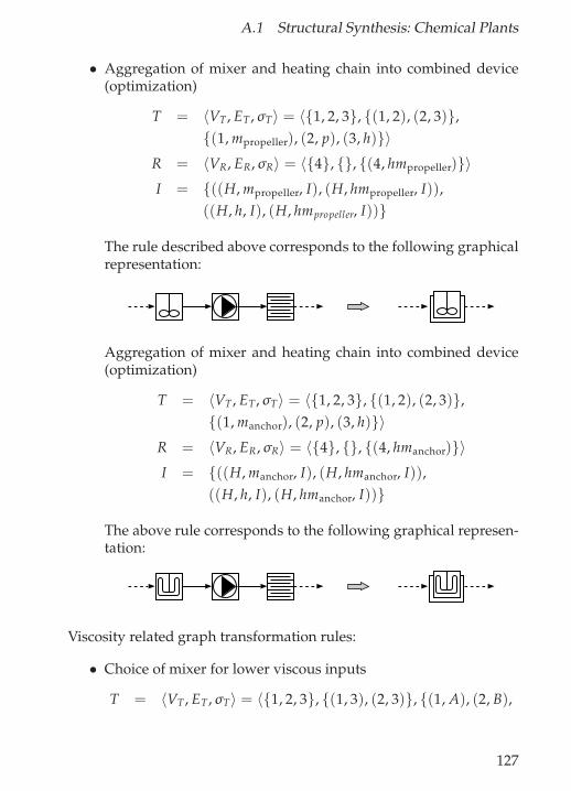
A.1 Structural Synthesis: Chemical Plants
• Aggregation of mixer and heating chain into combined device(optimization)
T = 〈VT , ET ,σT〉 = 〈{1, 2, 3}, {(1, 2), (2, 3)},{(1, mpropeller), (2, p), (3, h)}〉
R = 〈VR, ER,σR〉 = 〈{4}, {}, {(4, hmpropeller)}〉I = {((H, mpropeller, I), (H, hmpropeller, I)),
((H, h, I), (H, hmpropeller, I))}
The rule described above corresponds to the following graphicalrepresentation:
Aggregation of mixer and heating chain into combined device(optimization)
T = 〈VT , ET,σT〉 = 〈{1, 2, 3}, {(1, 2), (2, 3)},{(1, manchor), (2, p), (3, h)}〉
R = 〈VR, ER,σR〉 = 〈{4}, {}, {(4, hmanchor)}〉I = {((H, manchor, I), (H, hmanchor, I)),
((H, h, I), (H, hmanchor, I))}
The above rule corresponds to the following graphical represen-tation:
Viscosity related graph transformation rules:
• Choice of mixer for lower viscous inputs
T = 〈VT , ET ,σT〉 = 〈{1, 2, 3}, {(1, 3), (2, 3)}, {(1, A), (2, B),
127

A Applications in Design
(3, ?), ((1, 2), vh)}〉R = 〈VR, ER,σR〉 = 〈{4, 5, 6}, {(4, 6), (5, 6)},
{(4, A), (5, B), (6, manchor), ((4, 6), vh)}〉I = {((H, A, I), (H, A, I)), ((H, B, I), (H, B, I)),
((H, C, I), (H, manchor, I))}
The following graphical rule represents the above formal rule:
A
?
B
vh
A
B
vh
Choice of mixer for high viscous inputs
T = 〈VT , ET,σT〉 = 〈{1, 2, 3}, {(1, 3), (2, 3)}, {(1, A), (2, B),(3, ?), ((1, 2), vl)}〉
R = 〈VR, ER,σR〉 = 〈{4, 5, 6}, {(4, 6), (5, 6)},{(4, A), (5, B), (6, mpropeller), ((4, 6), vh)}〉
I = {((H, A, I), (H, A, I)), ((H, B, I), (H, B, I)),((H, C, I), (H, mpropeller, I))}
The formal notation yields the following graphical rule:
A
?
B
vl
A
B
vl
128

A.1 Structural Synthesis: Chemical Plants
• Improvement of mixing properties by dealing with high viscousinputs separately
T = 〈VT , ET ,σT〉 = 〈{1, 2, 3}, {(1, 3), (2, 3)}, {(1, A), (2, B),(3, C), ((1, 2), vh), ((2, 3), vh)}〉
R = 〈VR, ER,σR〉 = 〈{4, 5, 6, 7}, {(4, 6), (5, 6), (6, 7)},{(4, A), (5, B), (6, C), (7, C),((4, 6), vh), ((5, 6), vh), ((6, 7), vh)}〉
I = {((H, A, I), (H, A, I)), ((H, B, I), (H, B, I)),((H, C, I), (H, 7, I))}
The formal notation yields the following graphical rule:
vh
A
B
Cvh
vhC
vh
A
B
vh C
• Improvement of mixing properties by heating high viscous input
T = 〈VT , ET ,σT〉 = 〈{1, 2, 3}, {(1, 3), (2, 3)}, {(1, A), (2, B),(3, C), ((1, 3), vh), ((2, 3), vl)}〉
R = 〈VR, ER,σR〉 = 〈{4, 5, 6, 7, 8}, {(4, 6), (5, 8), (6, 7),(7, 8)}, {(4, A), (5, B), (6, h), (7, p), (8, C),((4, 6), vh), ((5, 8), vl), ((7, 8), th)}〉
I = {((H, A, I), (H, A, I)), ((H, B, I), (H, B, I)),((H, C, I), (H, C, I))}
The graphical rule representing the above formal rule is as fol-lows:
129

A Applications in Design
A
C
B
vh
A
C
B
vh
vl vl
t h
Remarks. Please note that the substance property under considerationdetermines the types of structural manipulation that are necessary. Forinstance, all properties lead to splitting rules, the property “tempera-ture” is connected to optimization rules, and the property “viscosity”implies choice rules. Likewise, the other substance properties not cov-ered by the design graph grammar described above are also associatedwith specific structural transformations.
The rule set presented above suffices to generate graphs corre-sponding to simple chemical plants; any remaining “?” labeled nodesare superfluous and can be deleted—this could also have been doneby means of a design graph grammar rule.
130

A.2 Structural Simplification: Hydraulic Plants
A.2 Structural Simplification: Hydraulic Plants
The maintenance of hydraulic plants is a challenging job for present-day engineers. The size and complexity of hydraulic plants exceed thehuman capacity to manage them efficiently, thus making additionalsupport a necessity. In special, the design task “analysis” for diagnosispurposes is of importance.
In [Schulz, 1997, Stein and Schulz, 1998] the concept of hydraulicaxes plays a major role within the analysis of a hydraulic plant. Hy-draulic axes represent substructures within a hydraulic plant that per-form a function; the recognition of all hydraulic axes of a hydraulicplant yields the set of all functions present within the plant—in a cer-tain sense one could say the recognition of hydraulic axes is the recog-nition of the building blocks that compose the global plant. Figure A.1shows a hydraulic plant and its hydraulic axes.
Figure A.1: A hydraulic plant containing three hydraulic axes (shadedareas); the fourth area is shared by all axes.
The recognition of the hydraulic axes of a plant does not sufficeto fully analyze a hydraulic plant. Within the diagnosis context theknowledge about the relationships between the individual axes is es-sential for a precise statement concerning a faulty component, since a
131

A Applications in Design
defect within a hydraulic axis often influences the behavior of otheraxes, spreading the faulty behavior throughout the hydraulic plant.Thus, the relationship between each pair of hydraulic axes within ahydraulic plant must be considered. Figure A.2 shows the couplingsbetween the hydraulic axes depicted in Figure A.1.
sequential
serial
Figure A.2: Coupling of hydraulic axes.
The tasks described above—the recognition of hydraulic axes andof their relationship to each other—are efficiently solved by means ofpath search algorithms. This is due to the inherent structure of hy-draulic axes; each hydraulic axis possesses a pump, representing apressure source, some valves for control together with additional aux-iliary components, and cylinders and motors, representing the work-ing devices responsible for the output. However, hydraulic axes oftenpossess substructures that hinder a full recognition: circuit loops, deadbranches etc. Thus, a hydraulic circuit has to be simplified prior to ap-plying path searching methods; Figure A.3 illustrates the simplifica-tion process.
The following simple design graph grammar suffices to performthe transformation described by Figure A.3.
132

A.2 Structural Simplification: Hydraulic Plants
Figure A.3: Simplification of a hydraulic circuit by structural compres-sion and merging.
First, let the following assumptions be made:
• Supply elements, i. e., pumps and tanks, are designated by thelabel “p”,
• Working elements, i. e., cylinders and motors, are represented bythe label “w”,
• Control elements, i. e., valves, are designated by the label “v”,
• Junction nodes, also called Tri-Connections, are represented by thelabel “j”,
• and all other auxiliary elements are designated by the label “a”.
133

A Applications in Design
Let G = 〈Σ, P, s〉 be a design graph grammar for the structuralsimplification of hydraulic circuits where Σ = {p, w, v, j, a, s, H, I, J,K, L, M, N}, s is the initial symbol (unused here) and P = Pcompression∪Pmerging is the set of graph transformation rules.
Now, we first provide the compression related graph transforma-tion rules Pcompression:
1. Compression of dead branches
T = 〈VT, ET ,σT〉 = 〈{1, 2}, {{1, 2}}, {(1, a), (2, K)}〉R = 〈VR, ER,σR〉 = 〈{3}, {}, {(3, K)}〉I = {((J, K, H), (J, K, H))}
The graphical representation of this rule is as shown below.
L K L
2. Compression of chains
T = 〈VT , ET ,σT〉 = 〈{1, 2, 3}, {{1, 2}, {2, 3}},{(1, H), (2, a), (3, K)}〉
R = 〈VR, ER,σR〉 = 〈{4, 5}, {{4, 5}}, {(4, H), (5, K)}〉I = {((I, H, M), (I, H, M)), ((J, K, M), (J, K, M))}
The graphical representation of this rule is depicted below.
a KH KH
3. Compression of loops
T = 〈VT, ET ,σT〉 = 〈{1, 2, 3, 4}, {{1, 2}, {1, 3},{2, 4}, {3, 4}}, {(1, j), (2, a), (3, a), (4, j)}〉
R = 〈VR, ER,σR〉 = 〈{5}, {}, {(5, j)}〉I = {((H, j, I), (H, j, I))}
The graphical representation of this rule is illustrated below.
134

A.2 Structural Simplification: Hydraulic Plants
a
a
jj j
The set of graph transformation rules Pmerging is defined as follows:
1. Merging with working elements
T = 〈VT , ET ,σT〉 = 〈{1, 2}, {{1, 2}}, {(1, w), (2, K)}〉R = 〈VR, ER,σR〉 = 〈{3}, {}, {(3, w)}〉I = {((H, w, L), (H, w, L)), ((J, K, M), (J, w, M))}
The above formal representation is equivalent to the followinggraphical notation:
w K w
2. Merging with supply elements
T = 〈VT , ET,σT〉 = 〈{1, 2}, {{1, 2}}, {(1, p), (2, K)}〉R = 〈VR, ER,σR〉 = 〈{3}, {}, {(3, p)}〉I = {((J, K, M), (J, p, M))}
The graphical representation of the above graph transformationrule is as follows:
p K p
3. Merging with control elements
T = 〈VT , ET ,σT〉 = 〈{1, 2}, {{1, 2}}, {(1, v), (2, K)}〉R = 〈VR, ER,σR〉 = 〈{3}, {}, {(3, v)}〉I = {((H, v, M), (H, v, M)), ((J, K, N), (J, v, N))}
135

A Applications in Design
Again, the corresponding graphical representation is depictedbelow:
v K v
Remarks. Some of the above graph transformation rules possess iden-tical structures and differ only with respect to node and edge labels.In such cases one could argue that label classes would reduce the num-ber of graph transformation rules noticeably. For example, all mergingrules could be written as a single rule using label classes; however, theembedding instructions would have to be adapted to match the mostgeneral case.
136

A.3 Structural Synthesis: Hydraulic Plants
A.3 Structural Synthesis: Hydraulic Plants
Like the analysis task described in section A.2, structural synthesisalso represents a major challenge due to the same reasons. One wayto tackle this job is to use case-based reasoning techniques to derivesolutions from previously solved tasks. In [Stein and Hoffmann, 1999],Stein and Hoffmann introduce abstract building blocks that are com-bined to form new hydraulic plants; the concrete plant parts corre-sponding to the abstract building blocks are retrieved from a casedatabase and adapted accordingly. Figure A.4 illustrates this notion.
w w
c
c
s
Figure A.4: Example of a concrete hydraulic plant and its abstractbuilding block view.
The following design graph grammar generates feasible structuresconsisting of abstract building blocks; a subsequent case-based pro-cessing step can then convert these abstract structures into concretehydraulic circuits.
First, let the following assumptions be made:
• Functional units are labeled with “f”,
• Supply elements, i. e., pumps and tanks, are designated by thelabel “s”,
• Working elements, i. e., cylinders and motors, are represented bythe label “w”,
• Control elements, i. e., valves, are designated by the label “c”,
137

A Applications in Design
• Junction nodes, also called Tri-Connections, are represented by thelabel “t”,
• and all other auxiliary elements are designated by the label “b”.
Let G = 〈Σ, P, ?〉 be a design graph grammar for the structural syn-thesis of hydraulic circuits where Σ = {?, f , s, w, c, t, b, A, B}, ? is theinitial symbol and P is the set of graph transformation rules.
The graph transformation rules in P are as follows:
1. Generation of a functional unit
? f bb
s
2. Refinement of a functional unit into a hydraulic axis
f w bb
c
3. Removal of auxiliary node
b BA A B
4. Insertion of a further functional unit in series
f bb f bb f b
5. Insertion of a further functional unit in parallel
f bb
f bb
f ttb b
138

A.3 Structural Synthesis: Hydraulic Plants
6. Insertion of a further hydraulic axis in parallel
w bbw bb
w ttb b
7. Insertion of a further hydraulic axis in sequence
w bb
w
w
bb
ttb b
c
Finally, the appearance used for Figure A.4 is achieved by meansof an additional design graph grammar with the following four graphtransformation rules:
ww
ss
t cc
139

A Applications in Design
A.4 Model Reformulation: Wave Digital Structures
Wave digital structures (WDS) form a particular class of signal flowgraphs where the signals are linear combinations of the electric cur-rent and flow. WDS represent a concept to translate electrical circuitsfrom the electrical u/i-domain into the a/b-wave-domain; this trans-lation establishes a paradigm shift and is called, in terms of models,model reformulation. With respect to this concrete example, this refor-mulation is bound up with several advantages, which are addressedin [Fettweis, 1986].
When migrating from an electrical circuit towards a WDS, the un-derlying model is completely changed: The structure model of theelectrical circuit, Mu/i
S , is interpreted as a series-parallel graph withclosely connected components and transformed into an adaptor struc-ture, Ma/b
S .
Figure A.5 shows the reformulation of a series-parallel structuretree of an electrical circuit into a corresponding adaptor structure. Thenodes labeled by “s” and “p” indicate series and parallel connectionsin the circuit.
p
s
s
p1 2
3 4 5
6 7
8 9
1
2
8
9
3
4
5
6
7
p
s Series connection
Parallel connection
Series adaptor
Parallel adaptor
Figure A.5: Overview of the mapping Mu/iS −→ Ma/b
S .
The following design graph grammar2 performs the model refor-mulation depicted in Figure A.5 for arbitrary structure models Mu/i
S .2Since the involved transformation is a translation rather than generation, it would be
better to speak of graph transformation systems instead of graph grammars.
140

A.4 Model Reformulation: Wave Digital Structures
G = 〈Σ, P, z〉 with Σ = {z, p, s, i, X, Y, A, B, C, D, E, F, G, H, I, J},z is the initial symbol (can be neglected), and P is the set of graphtransformation rules, which are presented in the following.
1. Splitting rule for nodes with more than three edges.
T = 〈VT, ET ,σT〉 = 〈{1, 2, 3, 4, 5}, {{1, 5}, {2, 5},{3, 5}, {4, 5}}, {(1, E), (2, F), (3, G), (4, H),(5, X), ({1, 5}, B), ({2, 5}, A), ({3, 5}, C),({4, 5}, D)}〉
R = 〈VR, ER,σR〉 = 〈{6, 7, 8, 9, 10, 11},{{6, 7}, {7, 8}, {7, 9}, {9, 10}, {9, 11}},{(6, F), (7, X), (8, E), (9, X), (10, G), (11, H),({6, 7}, A), ({7, 8}, B), ({7, 9}, i), ({9, 10}, C),({9, 11}, D)}〉
I = {((F, X, A), (F, 7, A)), ((E, X, B), (E, 7, B)),((G, X, C), (G, 9, C)), ((H, X, D), (H, 9, D)),((I, E, J), (I, E, J)), ((I, F, J), (I, F, J)),((I, G, J), (I, G, J)), ((I, H, J), (I, H, J))}
For illustrative reasons we resort to the graphical representationfrom now on and refrain from using the formal version if appro-priate.
X XiX
A
BC
DC
D
A
B
E
F
G
H
E
F
G
H
2. Marking rule for edges connecting inner nodes.
141

A Applications in Design
X Y YXi
A B A B
The above rules are sufficient to perform the structural transforma-tion required. The following rules belonging to an additional designgraph grammar are necessary to change the appearance of the finalstructure into an adaptor structure as depicted in Figure A.5.
1. Display of a parallel node.P
2. Display of a serial node.S
3. Display of a port node.X
X
Z
Z
4. Display of node connector.X
Xi
A A
142

A.5 Model Reformulation: Parallel-Series Graphs
A.5 Model Reformulation: Parallel-Series Graphs
Model reformulation, as motivated in section A.4, occurs in variousforms and within different contexts; however, many of them share thesame basic prerequisites and goals. The model reformulation task oftranslating a structure description tree, such as the one depicted byFigure A.5, into a parallel-series graph represents an adequate abstrac-tion of the corresponding tasks within concrete technical domains.
In a certain sense the goal of this model reformulation task is totranslate the structural view of the system of interest into its topolog-ical view. The initial structure is a structure description tree: Innernodes represent either parallel or serial parts of the described struc-ture, leaves represent edge labels. Figure A.6 shows a structure de-scription tree and the corresponding parallel-series graph.
pR
p
ss
∆∆ ∆
∆ ∆
∆
∆
∆∆
∆
Figure A.6: A structure description tree and its corresponding paral-lel-series graph.
The following design graph grammar performs the transformationrequired by the model reformulation task.
G = 〈Σ, P, z〉 with Σ = {z, pR, sR, p0, s0, p′, s′, e, l, r, ∆, A, B, H, I, J,K, L, M}, z is the initial symbol (can be neglected), and P is the set ofgraph transformation rules, which are presented in the following.
1. Initial rule for parallel rooted description tree
T = 〈VT, ET ,σT〉 = 〈{1}, {}, {(1, pR)}〉R = 〈VR, ER,σR〉 = 〈{2, 3, 4}, {{2, 3}, {3, 4}},
143

A Applications in Design
{(2, p0), (3, p′), (4, p0), ({2, 3}, l), ({3, 4}, r)}〉I = {((H, pR, I), (H, p′, I))}
The rule formally described above corresponds to the followinggraphical representation:
pR p'p0 p0l r
2. Initial rule for serial rooted description tree
T = 〈VT , ET,σT〉 = 〈{1}, {}, {(1, sR)}〉R = 〈VR, ER,σR〉 = 〈{2, 3, 4}, {{2, 3{, {3, 4}},
{(2, s0), (3, s′), (4, s0), ({2, 3}, l), ({3, 4}, r)}〉I = {((H, sR, I), (H, s′, I))}
The graphical representation of the above rule is as follows:
sR s's0 s0l r
3. Creation of parallel threads
T = 〈VT, ET ,σT〉 = 〈{1, 2, 3, 4}, {{1, 2}, {2, 3}, {2, 4}},{(1, A), (2, p′), (3, B), (4, s), ({1, 2}, l), ({2, 3}, r)}〉
R = 〈VR, ER,σR〉 = 〈{5, 6, 7, 8}, {{5, 6}, {5, 7}, {6, 8},{7, 8}}, {(5, A), (6, p′), (7, s′), (8, B),({5, 6}, l), ({5, 7}, l), ({6, 8}, r), ({7, 8}, r)}〉
I = {((H, p′, I), (H, p′, I)), ((H, s, I), (H, s′, I)),((H, A, I), (H, A, I)), ((H, B, I), (H, B, I))}
The above rule corresponds to the following graphically:
144

A.5 Model Reformulation: Parallel-Series Graphs
p'
s
p'
s'
l rl r
l r
A B
A B
Creation of parallel threads containing a leaf node
T = 〈VT, ET ,σT〉 = 〈{1, 2, 3, 4}, {{1, 2}, {2, 3}, {2, 4}},{(1, A), (2, p′), (3, B), (4, ∆), ({1, 2}, l), ({2, 3}, r)}〉
R = 〈VR, ER,σR〉 = 〈{5, 6, 7, 8}, {{5, 6}, {5, 7}, {6, 8},{7, 8}}, {(5, A), (6, p′), (7, ∆), (8, B),({5, 6}, l), ({5, 7}, l), ({6, 8}, r), ({7, 8}, r)}〉
I = {((H, p′, I), (H, p′, I)), ((H, A, I), (H, A, I)),((H, B, I), (H, B, I))}
The graphical representation is:
p'p'l r
l r
l r∆
∆
A B
A B
4. Removal of empty parallel node
T = 〈VT , ET ,σT〉 = 〈{1, 2, 3}, {{1, 2}, {2, 3}},{(1, A), (2, p′), (3, B), ({1, 2}, l), ({2, 3}, r)}〉
R = 〈VR, ER,σR〉 = 〈{4, 5}, {}, {(4, A), (5, B)}〉I = {((H, A, L), (H, A, L)), ((H, B, L), (H, B, L))}
The formal definition of the above rule conforms with the fol-lowing graphical representation:
145

A Applications in Design
p'l r
A B A B
5. Creation of serial thread
T = 〈VT , ET ,σT〉 = 〈{1, 2, 3, 4}, {{1, 2}, {2, 3},{2, 4}}, {(1, A), (2, s′), (3, B), (4, p),({1, 2}, l), ({2, 3}, r)}〉
R = 〈VR, ER,σR〉 = 〈{5, 6, 7, 8, 9}, {{5, 6}, {6, 7},{7, 8}, {8, 9}}, {(5, A), (6, p′), (7, e), (8, s′),(9, B), ({5, 6}, l), ({6, 7}, r), ({7, 8}, l), ({8, 9}, r)}〉
I = {((H, s′, I), (H, s′, I)), ((H, p, I), (H, p′, I)),((H, A, I), (H, A, I)), ((H, B, I), (H, B, I))}
The graphical rule depicted below reflects the above formal def-inition:
p
s'l r
A B
p' s'l r
A Bl r
e
Creation of a serial thread containing a leaf node
T = 〈VT , ET ,σT〉 = 〈{1, 2, 3, 4}, {{1, 2}, {2, 3},{2, 4}}, {(1, A), (2, s′), (3, B), (4, ∆),({1, 2}, l), ({2, 3}, r)}〉
R = 〈VR, ER,σR〉 = 〈{5, 6, 7, 8, 9}, {{5, 6}, {6, 7},{7, 8}, {8, 9}}, {(5, A), (6, ∆), (7, e), (8, s′),(9, B), ({5, 6}, l), ({6, 7}, r), ({7, 8}, l), ({8, 9}, r)}〉
I = {((H, s′, I), (H, s′, I)), ((H, A, I), (H, A, I)),((H, B, I), (H, B, I))}
146
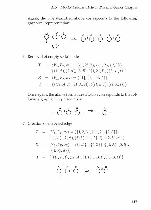
A.5 Model Reformulation: Parallel-Series Graphs
Again, the rule described above corresponds to the followinggraphical representation:
s'l r
∆
A Bs'
l r∆A Be
r l
6. Removal of empty serial node
T = 〈VT , ET ,σT〉 = 〈{1, 2∗, 3}, {{1, 2}, {2, 3}},{(1, A), (2, s′), (3, B), ({1, 2}, l), ({2, 3}, r)}〉
R = 〈VR, ER,σR〉 = 〈{4}, {}, {(4, A)}〉I = {((H, A, I), (H, A, I)), ((H, B, I), (H, A, I))}
Once again, the above formal description corresponds to the fol-lowing graphical representation:
l rs'A B A
7. Creation of a labeled edge
T = 〈VT , ET,σT〉 = 〈{1, 2, 3}, {{1, 2}, {2, 3}},{(1, A), (2, ∆), (3, B), ({1, 2}, l), ({2, 3}, r)}〉
R = 〈VR, ER,σR〉 = 〈{4, 5}, {{4, 5}}, {(4, A), (5, B),({4, 5}, ∆)}〉
I = {((H, A, I), (H, A, I)), ((H, B, I), (H, B, I))}
l r∆
∆A B A B
147

A Applications in Design
Remarks. As with the rules presented in section A.2, the use of labelclasses would result in a smaller rule set by combining all graph trans-formation rules with identical oder nearly identical structures. Again,the embedding instructions would have to be adapted to match themost general case.
Example. Figure A.7 illustrates the usage of the design graph grammardescribed above.
Remarks. This design graph grammar allows for parallelism, whichwas implicitly used in the derivation shown in Figure A.7.
148

A.5 Model Reformulation: Parallel-Series Graphs
pR
p
ss
∆∆ ∆
∆ ∆
p
ss
∆∆ ∆
∆ ∆
p'p0 p0l r
p
s
s'
∆
∆ ∆
∆ ∆
p'p0 p0
l r
l r
p
s'
s'
∆
∆
∆
∆ ∆
p'p0 p0
l r
l r
l r
∆∆
∆
∆
p0 p0
lr
e
∆
e
∆∆
∆∆
p0 p0
e
∆
e
p' s'
s'
∆∆
∆ ∆
p0 p0
l
r
l r
el
r
∆
e
lr
p'
∆∆
∆
∆p0 p0
l
r
lr
e
∆
e
lr
l
r
Figure A.7: Translation of a structure description tree into a parallel-series graph.
149
Index
algorithmanalysis-step, 41–42synthesis-step, 52–53
compilation, 60connecting approach, 74–77context, 23–24context graph, see graphcut nodes, 28
deletion operation, 106, 106, 107,110
derivation, 30, 104, 105, 108leftmost, 93, 93–94, 95rule sequence, 106shortest, 104, 105, 107, 108step, 30
design graph grammarboundary, 94–95, 95context-free, 29–30context-sensitive, 32–33
design process, 39
embedding instructions, 29
gluing approach, 77–79graph
context, 28host, 28labeled, 22ordered, 93replacement, 28rooted flowgraph, 101target, 28
graph distancederivational, 108–110direct, 108
graph grammargraph-based, 33–34NCE, 74, 75, 76–77, 100neighborhood uniform, 31NLC, 74, 74–75, 100node-based, 33–34precedence, 96, 100, 101
graph isomorphism, 22–23with labels, 22–23
graph isomorphism problem, 88
host graph, see graphHR grammar, 78
label alphabet, 29label distance, 58language
flowgraph, 101rooted context-free flow-
graph, 100location specifier, 65
matching, 23–24, 86strict degree, 24
maximal common subgraph prob-lem, 110
membership problem, 41, 43, 95,100
model simplification, 7approximation, 9behavioral simplification, 9
150

Index
causal decomposition, 9, 55derived relationships, 11entity aggregation
by function, 10by structure, 11
function aggregation, 11limited input space, 9model boundary simplifica-
tion, 7model context, 8numeric representation, 10simple task assumption, 7state aggregation, 10temporal aggregation, 10
modificationcharacteristics, 64global, 64local, 64parameter, 64
ordered spanning tree, 101
PGRS, 85, 105principle of least commitment, 37productions, 29property
associativity, 91confluence, 91, 100finite Church Rosser, 100monotonicity, 106–107, 110shortcut-free, 107
replacement graph, see graph
subgraph isomorphism problem,88
subgraph matching problem, 43,55, 86, 88, 95, 99, 110
target graph, see graph
transformation rules, see produc-tions
variable label, 29bound, 37unbound, 37
151