Lectures on the beginnings of calculus in Kerala and in Europe

Math 191, April 5, 7, 12, 14, 19

The School of Mādhava in Kerala, c.1350‐1600 CE

• Exodus of Brahmins from North following Muslim invasions (Delhi Sultanate, MughalEmpire of Babur, Akbar, etc.)

• Tightly knit guru‐parampara (“chain of teachers”): Mādhava (the founder) →Parameśvara→Dāmodara→Nīl k h J h d → N ( B h i !→Nīlakantha, Jyeșthadeva→ Narayana (+ non‐Brahmins! Śankara Variyar, Acyuta Pisārati)

• All in a small area, at small village temples, underAll in a small area, at small village temples, under protection of the Mahārājah of Calicut.

• Jyeșthadeva wrote a unique book, informal ‘lecture t ’ i M l l th Y kti Bhā ( lnotes’, in Malayalam, the Yukti‐Bhāșa (vernacular 

<exposition> of rationales). A translation by K. V. Sarmawas recently  published as Ganita‐Yukti‐Bhāșa.

• The basic ideas were attributed to Mādhava , and ideas such as a virtually heliocentric model of the solar system to Nīlakantha (1444‐c 1540)to Nīlakantha (1444‐c.1540)

• Their work never spread and was forgotten until c.1820 when C.M.Whish learned Malayalam, collected palm‐leaf manuscripts from Kerala and found, to his astonishment, a “complete system of fluxions”

• First big discovery: 1

1

R nn

nRx dx

• In §6.4 of the Yukti: “Summation of Series”

• Goal is to approximate the Riemann sum

0

Goal is to approximate the Riemann sum

b “ ll (“ ”)” hil

1

. , , "radius", "segment"n

p

ks k s ns R s

as s becomes “as small as an atom (“aņu”)” while n becomes as large as “parārdha” (1 trillion!)

• Now 1n n

p p pk k • Now

so the sums of integers are the key and he says:

1

1 1. p p p

k ks k s s k

so the sums of integers are the key and he says:

“Now suppose the radius to be the same number of units as the number of segments to which it has been divided, in order f g ,to facilitate remembering their number”,i.e. make s =1.

“ h h d d h f b f

To give the flavor, here’s the case p=3.

“Now, to the method or deriving the summation of cubes: Summation of cubes, it is clear, is the summation where the square of each  number (bhuja) in the summation of squares is multiplied by the number. Now, by how much will the sum of cubes increase if all the numbers squared were to be multiplied by the radius. By the principle enunciated earlier, the square number next‐to‐last will increase by itself being multiplied by 1. The square numbers below will increase by multiples of 2,3, etc. in order. That sum will be equal to the summation of summation of squares. It has already been shown that the summation of squares is equal to ⅓ the cube of the radius. Hence ⅓ the cube of each number will be equal to the summation of all square numbers ending with that number. Hence it follows that the summation of summation of square numbers is equal to ⅓ the sum of cube f f q q fnumbers. Therefore the summation of squares multiplied by the radius will be equal to the summatiuon of cubes plus ⅓ of itself. Hence, when ¼ of it is subtracted, what remains will be the summation of cubes. Hence, it also , f ,follows that the summation of cubes is equal to ¼ the square of the square of the radius.

3 2 2 ( ( ))R R R

k k k k R R k 1 1 1

2 2

. .( ( ))

R R

k k k k R R k

R k k

2 2

1 1 1

3 3

k

R

R k k

R

1 .

3 3

RRR

4 43 34 ,

3 3 4R Rk k

1 1

1

Same argument shows:p pn

p n R

1

1 . . . , equality

1 1p p

k

n Rs k s sp p

in the limit

Using double integrals and induction, this becomes:R R R R R 1 1 1

0 0 0 0

( ( )) .R R R R R

p p p p

x

x dx x R R x dx R x dx x dy dx

1

0 1

.p

p

x y

RR x dxdyp

0 1

x yp

1 = .yRp

pRR x dx dy

0 0

=Rp p

p

R yR dy

0

1 11

= .

1 hR Rp p

p p

R dyp p

R Rd d

1

0 0

so 1 , hence 1

p pp

R Rx dx x dxp p

He applies this summation tosummation to compute first 

1 1 11p= - + - +

in §6.3 and later to get the power series

4 3 5 7+ +

get the power series for arctan(x), any x.Here is his basic diagram, a quadrant of a circle of radius R P the “East”R, P the  East  point, the line PPndivided in a very large number n of segments

“Now is described the procedure for arriving at theNow is described the procedure for arriving at the circumference of a circle of desired diameter without involving calculation of square roots. Construct a square with four sides equal to the diameter of the proposed circle. Inscribe the circle inside the square in such a manner that the circumference of that circle touches the centers of the f f ffour sides of the square. Them through the center of the circle, draw the east‐west line and the north‐south line with their tips being located at the points of contact of thetheir tips being located at the points of contact of the circumference and the sides. Then the interstice between the east‐point and the south‐east corner of the square will be equal to the radius of the circle. Divide this line into a number of equal parts by marking a large number of points closely at equal distances. The more the divisions, the more y q ,accurate would be the calculated circumference.”

Outline of proof:

Let 1R s n s P P i n k OP

p

1

1

Let . , , 1 , ,

angle , so that 8

i i i in

i i i i

R s n s P P i n k OP

P OP

1

Sections 6.3.1, 6.3.2 are devoted to showing:i

R R

21

sin( ).

i i ( )

i ii i i

s R s Rk k k

P P R

d l P P0or, since is arctan( ), i iP P x R x 0

2 2 2

coord along ,

he shows

nP Pd R Rd k R

2 2 2dx k R x

“6.3.1: Dividing the circum into arc‐bits

APi Pi+1

C´Qicircum. into arc‐bits, approx. the arc‐bits by sines” C

C˝

Δ(AOPi+1) congruent toΔ(ACPi+1) and to  θi+1Δ(PiC´Pi+1) andΔ(PiC´O) congruent to Δ(QiC˝O)

θi

Δ(QiC O).Thus:

Oi iC P C PR OA O

1 1 1

and sin( ) hence sin( )

i i i i

i i i

k sOP PP

C P C P C Q s R

1

and sin( ), hence sin( )i ii i ii ik k kOP OP

Last step:

Start with the identity:a a ac

( )

and iterate, giving the "sequence of subtractive corrections":b c b b b c

2 2 3

2 2 2 3 4( )a a ac ac a ac ac ac

b c b b b b c b b b b

Applying this to a

2 2 2

3 2 5 4

. , , ( ) , ,is R b R c is b c k

s R s s i s i

2 3 5

3 3 5 5

.4

1 1 1

ii i ii

s R s s i s ik R R R

3 3 5 5

3 5

1 1 1 13 3 5 7

sn s n s nR R R

How rigorous is this?

• Bounds comparing                         are easy and strong

,p pk x strong

• Bounds on                         are also easy

A i k i h

sin( ) 1 1 11• A tricky part is that                                   

converges only conditionally, not absolutely

1 1 13 5 71

• If x < 1, then we get absolute convergence for3 5

3 5arctan( ) x xx x

This is called “Abel summation”: that the limit of this as x→1 can be taken term by term.

3 5

of this as x→1 can be taken term by term.

It is interesting to compare this argument with Newton’sthis argument with Newton s  derivation of Kepler’s Second Law: that planets move so that the area swept out the line connecting them to the sun increases at a constant su c eases at a co sta tspeed. Both use geometry in discrete approximations, then a loose passage to thethen a loose passage to the limit.

Isaac Newton, Philosophiæ Naturalis Principia Mathematica, 1687

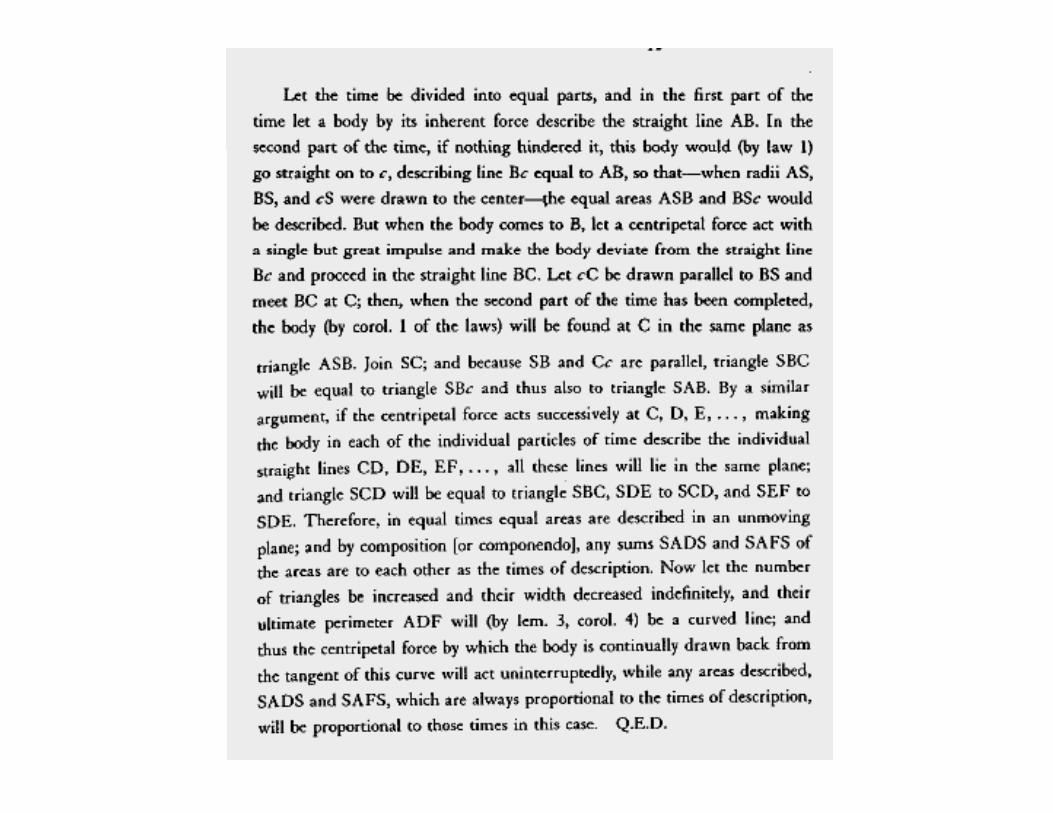
How did Newton justify his methods (my bold face)

“In any case, I have presented these lemmas before the propositions in order to avoid the tedium of working out lengthy proofs by reductio ad absurdum in the manner of the ancient geometers. Indeed, proofs are rendered more concise by g , p ythe method of indivisibles. But since the hypothesis of indivisibles is problematical and this method is accounted less geometrical, I have preferred to make the proofs of what follows depend on the ultimate sums and ratios of vanishing quantities and on the first sums and ratios of nascent quantities, that is, on the limits of such sums and ratios, and therefore to present proofs of those limits beforehand as briefly as I could. For the same result is obtained by h b h h d f d bl d h ll b f dthese as by the method of indivisibles, and we shall be on safer ground using principles that have been proved. ….

It may be objected that there is no such thing as an ultimate proportion ofIt may be objected that there is no such thing as an ultimate proportion of vanishing quantities, inasmuch as before vanishing the proportion is not ultimate, and after vanishing it does not exist at all. But the answer is easy: … the ultimate ratio of vanishing quantities is to be understood not as the ratio ofthe ultimate ratio of vanishing quantities is to be understood not as the ratio of quantities before they vanish or after they have vanished but the ratio with which they vanish.”

Nicole Oresme, 1323‐1382, Tractatus de Configurationibus Qulaitatum

One thing he was very clear about is that the keything about a graph is that its shape should depict

t l th ti f th lit b iaccurately the ratios of the quality beingmeasured against the true distances in the subject,an interval of space or timean interval of space or time.

This is the point in problem #1, HW9.

Gottfried Wilhelm von Leibniz, 1646‐1716• Polymath: Philosopher, Mathematician, Scientist, he aspired to understand everything and reduce to a p y glogical system

• Discovered calculus seemingly independently of Newton, drawing on many ideas ‘in the air’ in the work of Fermat, Descartes, Cavalieri, Huygens, P l BPascal, Barrow

• Introduced                                  and the formalism for ki ith th b i t l ti t d b

, (also )dx x ddxworking with them., being strongly motivated by finite differences of discrete sequences, as were the Indian mathematiciansIndian mathematicians.

If A, B, C, D, E are supposed to be quantities that continually pp q yincrease in magnitude, and the differences between successive terms are denoted by L, M, N, P, it will follow that

L+M+N+P = E-AL+M+N+P = E Athat is, sums of the differences, no matter how great their number, will be equal to the difference between terms at the beginning and 

d f h i F l l k h 0 1 4 9 16 25end of the series. For example, let us take the squares 0 1 4 9 16 25 with differences 1 3 5 7 9. It is evident that

1+3+5+7+9 = 25-0 = 25and the same will hold good whatever the number of terms or the differences may be. Delighted by this easy elegant theorem, our young friend considered a large number of numerical series andyoung friend considered a large number of numerical series, and also proceeded to to the second differences or differences of the differences, ….

• Leibniz wrote many unpublished notes and many letters.

• In an unpublished manuscript addressed to the the“Journal des Savans” (from the 1670’s), he announces

1 1 114 3 5 7p= - + - +

by a method which starts very differently from Madhavan but ends the same way [next slide]

• He publishes New Method for Maxima Minima and• He publishes New Method for Maxima, Minima and Tangents in 1784 using differentials dx and showing how to calculate dy/dx for all functions y=f(x) obtained y y f( )by rational expressions and powers. 

• His notes and letters show much more detail including i t l th f d t l th d hi hintegrals, the fundamental theorem and even higher order differentials ddx, dddx, … [describe]