on the bv-formalism - math.uni-hamburg.de · on the bv-formalism thanks while banging my head...
TRANSCRIPT

On the BV-formalism
On the BV-formalism
Urs Schreiber
January 17, 2008
Urs Schreiber On the BV-formalism
On the BV-formalism
Abstract
We try to understand theBatalin-Vilkovisky (BV) complex for handling perturbativequantum field theory.I emphasize a Lie ∞-algebraic perspective based on[Roberts-S., Sati-S.-Stasheff] over the popular supergeometryperspective and try to show how that is useful.A couple of examples are spelled out in detail:
the (−1)-brane;ordinary gauge theory;higher gauge theory.
Using these we demonstrate that the BV-formalism arisesnaturally from a construction ofconfiguration space from an internal hom-objectfollowing in spirit, but not in detail, the very insightful [AKSZ,Roytenberg].
Urs Schreiber On the BV-formalism

On the BV-formalism
Thanks
While banging my head against the BV-formalism, I profited fromconversation with
John Baez
Dmitry Roytenberg
Pavol Severa
Jim Stasheff
Danny Stevenson
Zoran Skoda
Todd Trimble
Of course none of them can be taken responsible for what is wrongand/or idiosyncratic about my presentation, as far as it is.The discussion of the higher gauge theory example is based on[Baez-S., S.-Waldorf, Sati-S.-Stasheff].
Urs Schreiber On the BV-formalism

On the BV-formalism
Plan
1 Introduction
2 ∞-vector spaces: (co)chain complexes
3 Lie ∞-algebras: differential graded (co)algebra
4 ∞-configuration spaces: the BV complex
Differential forms on spaces of mapsthe Chevalley-Eilenberg complexthe Koszul-Tate complexthe full BV-complex
5 Examples
6 Annotated literature
Urs Schreiber On the BV-formalism

On the BV-formalism
Introduction
IntroductionWhat is perturbative quantum field theory?
What is the BV-complex and what does it accomplish?
How can we understand that?
What is the relation to the Weil algebra of Lie n-algebroids?
How do we obtain BV-complexes?
next: ∞-vector spaces
Urs Schreiber On the BV-formalism

On the BV-formalism
Introduction
Field Theory
The setup of field theory
Classical field theory.
a “space” of configurations
conf
an “action functional”
exp(S) : conf → U(1)
Quantum field theory.
something like a measure
dµ
on confthe path integral ∫
confexp(S) dµ
Urs Schreiber On the BV-formalism
On the BV-formalism
Introduction
Field Theory
The problem and one of its solutions
Problem. conf is usually “two large” in two ways:
conf is typically not a finite dimensional manifold;
conf typically has many flows along which exp(S) is invariant,the symmetries.
One solution: perturbative quantum field theory
Taylor-expand S around critical points of S (the classicalsolutions);
inject conf into a supermanifold and extend exp(S) to asuperfunction such that the odd part of the path integral(over the ghosts) divides out the symmetries.
Urs Schreiber On the BV-formalism

On the BV-formalism
Introduction
The idea of BV-formalism
Tools to take care of that
Dealing with the symmetries.The BRST-complex is the Chevalley-Eilenberg complex ofthe symmetries acting on the module of functions on conf.In 0-th cohomology: the functions invariant under thesymmetries.
Dealing with the critical points.The Koszul-Tate complex is the weak quotient of allfunctions on conf by those that vanish on the critical pointsof S .In 0-th cohomology: the functions on the critical points of S .
Urs Schreiber On the BV-formalism

On the BV-formalism
Introduction
The idea of BV-formalism
BV-complex
The BRST complex and the Koszul-Tate complex happen to unifyto the Batalin-Vilkovisky (BV) complex
BV•(conf, exp(S)) .
If we think of conf as a supermanifold, then
the BV complex is the space of functions the shiftedcotangent bundle of conf, regarded as a supermanifold
BV• = C∞(T [1]∗conf) .
If we think of conf as a Lie n-algebroid, then
the BV complex is the space of horizontal inner derivations onthe Weil algebra of conf
BV• = horinn(W(conf)) .
Urs Schreiber On the BV-formalism

On the BV-formalism
Introduction
The role of Lie n-algebroids and Lie n-groupoids
It is useful to regard the BV-formalism as being aboutLie ∞-algebroids:
Urs Schreiber On the BV-formalism

On the BV-formalism
Introduction
The role of Lie n-algebroids and Lie n-groupoids
Sketches of the ∞-Lie theorem
Lie’s classical theorem says that every Lie algebra is the linearapproximation to some Lie group.People are progressing towards the many-object (Lie algebroid) andhigher dimensional (Lie n-algebroids) version of this:
∞-Lie theorem
L∞-algebra _
[Sullivan], [Getzler], [Henriques] // Lie ∞-groups _
Lie ∞-algebroids oo [Severa]
:=
Lie ∞-groupoids
:=
dg-manifolds oo // smoothKan-complexes
Urs Schreiber On the BV-formalism

On the BV-formalism
Introduction
The role of Lie n-algebroids and Lie n-groupoids
Underlying this are two classical results:
Fact (Dold-Kan, Brown-Higgins)
degree + 0 -ordinary
vector spaceChaincomplexes
are∞-vectorspaces.
interpretation ︸ ︷︷ ︸∞−vector space︸ ︷︷ ︸
∞−covector space
Fact (Sullivan models in rational homotopy theory)
Every non-negatively graded commutative differential A algebra isessentially the algebra of differential forms on some “space” XA
A → Ω•(XA) .
Urs Schreiber On the BV-formalism
On the BV-formalism
Introduction
The role of Lie n-algebroids and Lie n-groupoids
How to interpret the BV-complex
Using the ∞-Lie theorem, we can read the BV-formalism as saying
Observation
The configuration “space” of a physical system is really
a Lie ∞-groupoid:
objects are the physical configurations;morphisms are the gauge transformations betweenconfigurations;2-morphisms are the gauge-of-gauge transformations;n-morphisms are the n-fold gauge transformations.
Urs Schreiber On the BV-formalism

On the BV-formalism
Introduction
The role of Lie n-algebroids and Lie n-groupoids
The Lie ∞-algebraic interpretation of the BV-complex
BV-terminologyDGCA
interpretationLie ∞-groupoidinterpretation
fieldsdegree 0 generators
of CE(g, V )objects of
configuration spacefieldsandghosts
ghostsdegree 1 generators
of CE(g, V )morphisms in
configuration space
n-fold ghostsdegree n generators
of CE(g, V )n-morphisms in
configuration space
antifieldsdegree 1 horizontal
derivations in W(g, V )paths ofobjects
antifieldsand
antighostsantighosts
degree 2 horizontalderivations in W(g, V )
paths of1-morphisms
anti-ghosts-of-ghostsdegree 3 horizontal
derivations in W(g, V )paths of
2-morphisms
Urs Schreiber On the BV-formalism

On the BV-formalism
Introduction
Relation between the BV-complex and the Weil algebra
What is the relation between the BV complex and theWeil algebra of a Lie ∞-algebroid?
Urs Schreiber On the BV-formalism
On the BV-formalism
Introduction
Relation between the BV-complex and the Weil algebra
Lie ∞-algebras
A L∞-algebra g – the infinite categorification of a Lie algebra – is acodifferential graded co-commutative coalgebra
g = (∨•V ,Dg)
whose underlying graded co-commutative coalgebra is freelygenerated from a N+-graded vector space V .
Urs Schreiber On the BV-formalism
On the BV-formalism
Introduction
Relation between the BV-complex and the Weil algebra
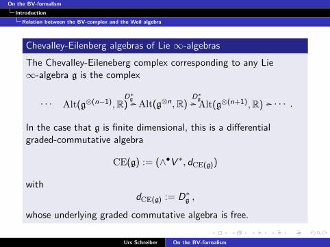
Chevalley-Eilenberg algebras of Lie ∞-algebras
The Chevalley-Eileneberg complex corresponding to any Lie∞-algebra g is the complex
· · · Alt(g⊗(n−1), R)D∗
g // Alt(g⊗n, R)D∗
g// Alt(g⊗(n+1), R) // · · · .
In the case that g is finite dimensional, this is a differentialgraded-commutative algebra
CE(g) := (∧•V ∗, dCE(g))
withdCE(g) := D∗
g ,
whose underlying graded commutative algebra is free.
Urs Schreiber On the BV-formalism

On the BV-formalism
Introduction
Relation between the BV-complex and the Weil algebra
In fact, every differential graded-commutative algebra DGCAwhose underlying graded commutative algebra is free on a finitedimensional N+-graded vector space comes from a finitedimensional L∞-algebra this way.
Urs Schreiber On the BV-formalism
On the BV-formalism
Introduction
Relation between the BV-complex and the Weil algebra
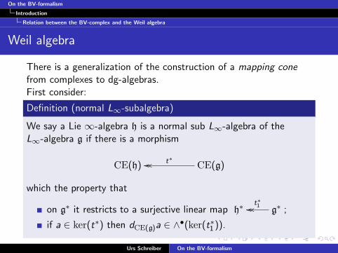
Weil algebra
There is a generalization of the construction of a mapping conefrom complexes to dg-algebras.First consider:
Definition (normal L∞-subalgebra)
We say a Lie ∞-algebra h is a normal sub L∞-algebra of theL∞-algebra g if there is a morphism
CE(h) CE(g)t∗oooo
which the property that
on g∗ it restricts to a surjective linear map h∗ g∗t∗1oooo ;
if a ∈ ker(t∗) then dCE(g)a ∈ ∧•(ker(t∗1 )).
Urs Schreiber On the BV-formalism
On the BV-formalism
Introduction
Relation between the BV-complex and the Weil algebra
Proposition
For h and g ordinary Lie algebras, the above notion of normal subL∞-algebra coincides with the standard notion of normal sub Liealgebras.
Urs Schreiber On the BV-formalism

On the BV-formalism
Introduction
Relation between the BV-complex and the Weil algebra
Weil algebra
Definition (mapping cone of qDGCAs; crossed module of normalsub L∞-algebras)
Let t : h → g be an inclusion of a normal sub L∞-algebra h intog. The mapping cone of t∗ is the qDGCA whose underlying gradedalgebra is ∧•(g∗ ⊕ h∗[1])
and whose differential dt is such that it acts on generatorsschematically as
dt =
(dg 0t∗ dh
).
The mapping cone L∞-algebra thus obtained we denote
(ht
→ g) .
Urs Schreiber On the BV-formalism
On the BV-formalism
Introduction
Relation between the BV-complex and the Weil algebra
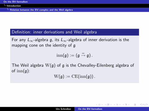
Definition: inner derivations and Weil algebra
For any L∞-algebra g, its L∞-algebra of inner derivation is themapping cone on the identity of g
inn(g) := (g=→ g) .
The Weil algebra W(g) of g is the Chevalley-Eilenberg algebra ofof inn(g):
W(g) := CE(inn(g)) .
Urs Schreiber On the BV-formalism

On the BV-formalism
Introduction
Relation between the BV-complex and the Weil algebra
The Weil algebra turns out to be trivializable, and yet, partlybecause of that, it is of crucial importance.
Observation (Weil algebra and shifted tangent bundle
If we regard CE(g) from the point of view of supermanifolds as thealgebra of functions on a supermanifold Xg, then W(g) is thealgebra of functions on the shifted tangent bundle T [1]Xg of Xg:
W(g) = C∞(T [1]Xg) .
Recall that the BV-complex can be thought of as the shiftedcotangent bundle of a supermanifold.
Urs Schreiber On the BV-formalism
On the BV-formalism
Introduction
Relation between the BV-complex and the Weil algebra
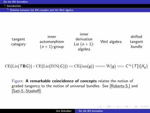
tangentcategory
innerautomorphism(n + 1)-group
innerderivation
Lie (n + 1)-algebra
Weil algebrashiftedtangentbundle
CE(Lie(TBG )) CE(Lie(INN(G ))) CE(inn(g)) W(g) C∞(T [1]Xg)
Figure: A remarkable coincidence of concepts relates the notion ofgraded tangency to the notion of universal bundles. See [Roberts-S.] and[Sati-S.-Stasheff].
Urs Schreiber On the BV-formalism

On the BV-formalism
Introduction
Obtaining BV-complexes from inner homs
With that nice interpretation in hand, the question remains how weextract from a given physical setup the relevant configuration Lie∞-groupoid such that its Lie n-algebroid supports a BV-complex.In [AKSZ, Roytenberg] it was observed, more or less explicitly, thatthe entire BV-setup drops out, more or less automatically, if oneforms the configuration space object (for field theories of generalσ-model type) as the internal hom-object of maps from parameterspace to configuration space.We here adopt that general idea, but give a possibly different,systematic and conceptual, construction of the internal hom-object.
Urs Schreiber On the BV-formalism

On the BV-formalism
Introduction
Obtaining BV-complexes from inner homs
Internalized physics
For field theories of σ-model and of gauge theory type, we aredealing with objects
par – parameter space
tar – target space
phas – space of phases
in some ambient category T , together with a morphism
tra : tar→ phas – the background field
which we want to transgress to
conf := hom(par, tar) – the configuration space of fields ,
which is the internal hom-object of maps from par to tar in T .
Urs Schreiber On the BV-formalism

On the BV-formalism
Introduction
Obtaining BV-complexes from inner homs
Internalized physics
The situation is a diagram
maps(par, tar)⊗ par
vvvvnnnnnnnnnnnnnev
''PPPPPPPPPPPPP
par tar tra // phas
in T from which we build the action functional
exp(S) : 1→ hom(conf,maps(par, tar)) .
Urs Schreiber On the BV-formalism

On the BV-formalism
Introduction
Obtaining BV-complexes from inner homs
Example for internalized physics: ordinary gauge theory
A good concrete example of this to keep in mind is the example ofordinary gauge theory of g-connections on a manifold Y , which wediscuss in detail in Example: ordinary gauge theory.Here we are working with T the category of diferentialgraded-commutative algebras of non-negative degree. We set
Internalization of ordinary gauge theory
par = Ω•(Y ) – the algebra of forms on Y
tar = W(g) – the Weil algebra of g
conf = Ω•(U 7→ Hom(W(g)),Ω•(Y × U)) – the algebra offorms on the presheaf on manifolds (i.e. the generalizedsmooth space) of dg-morphisms from W(g) to Ω•(Y ).
Urs Schreiber On the BV-formalism

On the BV-formalism
Introduction
Obtaining BV-complexes from inner homs
Example for internalized physics: ordinary gauge theory
This specifies the kinematics of ordinary gauge theory. Wedemonstrate in Example: ordinary gauge theory that theconfiguration space object thus obtained does indeed support theBV complex in that it knows about all the fields, ghosts, antifieldsand antighosts.To do dynamics, we need to choose a “background field”tra : tar→ phas. A good example to keep in mind for this istopological Yang-Mills theory with action functional
(A ∈ Ω•(Y , g)) 7→∫
Y〈FA ∧ FA〉 .
Urs Schreiber On the BV-formalism

On the BV-formalism
Introduction
Obtaining BV-complexes from inner homs
Example for internalized physics: ordinary gauge theory
This is obtained by taking
phas = CE(b3u(1)) – the Lie 4-algebra triply shifted u(1)
( tar oo tra phas ) = ( W(g) oo 〈·,·〉CE(b3u(1)) ) – the
embedding of the invariant polynomial 〈·, ·〉 into W(g).
Here I am making extensive use of the stuff discussed inSati-S.-Stasheff, which eventually I need to review here.Notice the reversal of the above arrows due to the fact that withalgebras everything is contravariant.
Urs Schreiber On the BV-formalism

On the BV-formalism
∞-Vector spaces: (co)chain complexes
previous: Introduction
∞-Vector spaces:(co)chain complexes
A-modules
Chain complexes as internal ω-categories
Cochain complexes of A-modules
next: Lie ∞-algebras
Urs Schreiber On the BV-formalism

On the BV-formalism
∞-Vector spaces: (co)chain complexes
The objects that we shall be concerned with here are differentialgraded algebras (dg-algebras). The right way to think of adg-algebra is as a monoid in a category of cochain complexes.
dg-algebra monoid in Ch•(A)
wedge product tensor product
graded-commutativity nontrivial symmetric braiding
Table: Realizing dg-algebras as monoids in chain complexes.
We recall very basic facts about the category of chain complexesand the homological algebra one can do with it.
Urs Schreiber On the BV-formalism

On the BV-formalism
∞-Vector spaces: (co)chain complexes
A-modules
A-modules
Urs Schreiber On the BV-formalism
On the BV-formalism
∞-Vector spaces: (co)chain complexes
A-modules
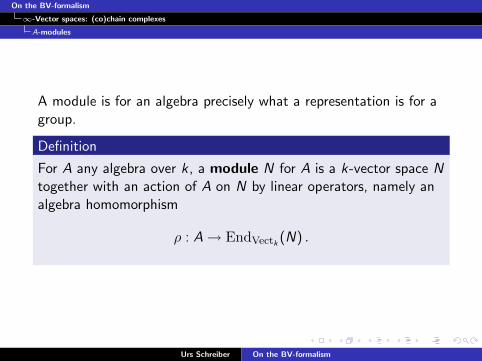
A module is for an algebra precisely what a representation is for agroup.
Definition
For A any algebra over k, a module N for A is a k-vector space Ntogether with an action of A on N by linear operators, namely analgebra homomorphism
ρ : A→ EndVectk (N) .
Urs Schreiber On the BV-formalism
On the BV-formalism
∞-Vector spaces: (co)chain complexes
A-modules
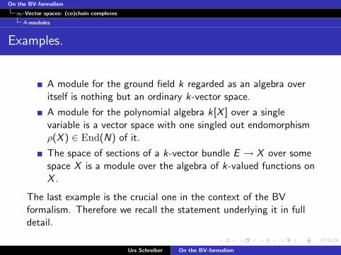
Examples.
A module for the ground field k regarded as an algebra overitself is nothing but an ordinary k-vector space.
A module for the polynomial algebra k[X ] over a singlevariable is a vector space with one singled out endomorphismρ(X ) ∈ End(N) of it.
The space of sections of a k-vector bundle E → X over somespace X is a module over the algebra of k-valued functions onX .
The last example is the crucial one in the context of the BVformalism. Therefore we recall the statement underlying it in fulldetail.
Urs Schreiber On the BV-formalism

On the BV-formalism
∞-Vector spaces: (co)chain complexes
A-modules
Definition (special properties of modules)
The following special properties of A-modules are important.
An A-module N is finitely generated if it is spanned, over A,by finitely many of its elements.
An A-module N is free of rank n ∈ N if it is of the formN ' An := A⊕n.
An A-module N is projective if any of the followingequivalent conditions hold
N is a direct summand of a free module, i.e. there existsanother module N ′ such that N ⊕ N ′ is free.N is the image N ' im(P) of a projection P ∈ End(An) onsome free module.
N satisfies the lifting property ∀g , f :
M ′
N
g //
∃h
>>
M
Urs Schreiber On the BV-formalism
On the BV-formalism
∞-Vector spaces: (co)chain complexes
A-modules
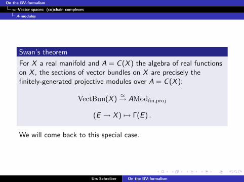
Swan’s theorem
For X a real manifold and A = C (X ) the algebra of real functionson X , the sections of vector bundles on X are precisely thefinitely-generated projective modules over A = C (X ):
VectBun(X )'→ AModfin,proj
(E → X ) 7→ Γ(E ) .
We will come back to this special case.
Urs Schreiber On the BV-formalism

On the BV-formalism
∞-Vector spaces: (co)chain complexes
A-modules
There is an obvious notion of homomorphisms of A-modules.
Definition
Given two A-modules N and N ′, an A-module homomorphism
f : N → N ′
between them is a linear map that preseves the A action:
A⊗ Nρ⊗Id //
IdA⊗f
End(N)⊗ Nev // N
f
A⊗ N ′ ρ′⊗Id // End(N ′)⊗ N ′ev // N ′
.
Urs Schreiber On the BV-formalism

On the BV-formalism
∞-Vector spaces: (co)chain complexes
A-modules
Definition (the category of A-modules)
We write AMod for the category whose objects are A-modules andwhose morphisms are A-module homomorphisms.
Urs Schreiber On the BV-formalism
On the BV-formalism
∞-Vector spaces: (co)chain complexes
A-modules
Structures and properties of AMod.
AMod is an abelian category, hence we can do homologicalalgebra inside AMod.Recall that this is equivalent to saying that that
it has a zero-object – this is the 0-dimensional A-module;and it has all pullbacks and pushouts;and all monomorphisms and epimorphisms are normal.
AMod is symmetric monoidal. The tensor product
⊗A : AMod× AMod→ AMod
is the ordinary tensor product of A-modules over A. Thetensor unit is I = A and the symmetric braiding is theobious one.
Urs Schreiber On the BV-formalism
On the BV-formalism
∞-Vector spaces: (co)chain complexes
A-modules
Structures and properties of AMod.
AMod is closed with respect to the above monoidal structure.The internal hom
hom : AModop × AMod→ AMod
sends any two A-modules to the vector space of A-modulehomomorphisms between them, equipped with an A-modulestructure in the obvious way.
Urs Schreiber On the BV-formalism

On the BV-formalism
∞-Vector spaces: (co)chain complexes
A-modules
Structures and properties of AMod.
AMod has duals. The dual
(−)∗ : AMod→ AModop
is(−)∗ = hom(−,A) .
The A-module V is of finite rank if (V ∗)∗ ' V .The full subcategory of finite rank modules we denote
AModfin .
AModfin is compact closed, meaning that the internal homexists and is
hom(V ,W ) ' V ∗ ⊗A W .
Urs Schreiber On the BV-formalism
On the BV-formalism
∞-Vector spaces: (co)chain complexes
A-modules
Example
In the context of Swan’s theorem, consider modules of functionalgebras given by sections Γ(E ) of vector bundles E → X oversome space X .Then:
The dual module V ∗ ' Γ(E ∗) is the space of sections of thedual bundle.
The tensor product V ⊗A W corresponds, under to theordinary fiberwise tensor product of vector bundles:
Γ(E )⊗C(X ) Γ(E ′) ' Γ(E ⊗VectBun E ′) .
Urs Schreiber On the BV-formalism

On the BV-formalism
∞-Vector spaces: (co)chain complexes
chain complexes as internal ω-categories
Chain complexes as internal ω-categories.
Urs Schreiber On the BV-formalism

On the BV-formalism
∞-Vector spaces: (co)chain complexes
chain complexes as internal ω-categories
One combinatorial model for higher dimensional homotopies areω-categories (strict, globular or cubical). The nerve of anω-category internal to AMod is a simplicial A-module.The famous Dold-Kan correspondence says that by forgetting lotsof face maps except one, and restricting it to the kernel of some ofthe other face maps, one obtains from a simplicial A-module anon-negatively graded chain complex of A-modules without loosinginformation.
Urs Schreiber On the BV-formalism

On the BV-formalism
∞-Vector spaces: (co)chain complexes
chain complexes as internal ω-categories
Dold-Kan correspondence
Forming the normalized chain complex from a simplicial A-moduleis an equivalence of categories
AMod∆op ' // Ch+• (AMod) .
Urs Schreiber On the BV-formalism

On the BV-formalism
∞-Vector spaces: (co)chain complexes
chain complexes as internal ω-categories
This equivalence is just the first in a longer list.
Brown and Higgins [?]
Let A be an abelian category. Then the following categories,internal to A, are all equivalent:
simplicial objects
chain complexes
crossed complexes
cubical sets with connections
cubical ω-groupoids with connections
globular ω-groupoids.
Urs Schreiber On the BV-formalism
On the BV-formalism
∞-Vector spaces: (co)chain complexes
chain complexes as internal ω-categories
Remark
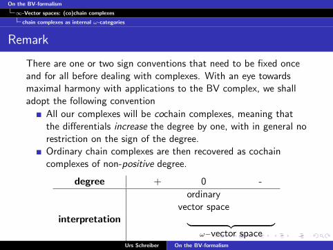
There are one or two sign conventions that need to be fixed onceand for all before dealing with complexes. With an eye towardsmaximal harmony with applications to the BV complex, we shalladopt the following convention
All our complexes will be cochain complexes, meaning thatthe differentials increase the degree by one, with in general norestriction on the sign of the degree.Ordinary chain complexes are then recovered as cochaincomplexes of non-positive degree.
degree + 0 -
ordinaryvector space
interpretation ︸ ︷︷ ︸ω−vector space︸ ︷︷ ︸
ω−covector space
Table: The interpretation of cochain complexes in terms of higherorder vector spaces.
Urs Schreiber On the BV-formalism
On the BV-formalism
∞-Vector spaces: (co)chain complexes
Cochain complexes of A-modules
Cochain complexes of A-modules
Urs Schreiber On the BV-formalism
On the BV-formalism
∞-Vector spaces: (co)chain complexes
Cochain complexes of A-modules
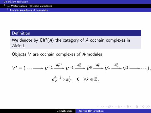
Definition
We denote by Ch•(A) the category of A cochain complexes inAMod.
Objects V are cochain complexes of A-modules
V • = ( · · · // V−2d−1
V // V−1d0
V // V 0d1
V // V 1d2
V // V 2 // · · · ) ,
dk+1V dk
V = 0 ∀k ∈ Z .
Urs Schreiber On the BV-formalism
On the BV-formalism
∞-Vector spaces: (co)chain complexes
Cochain complexes of A-modules
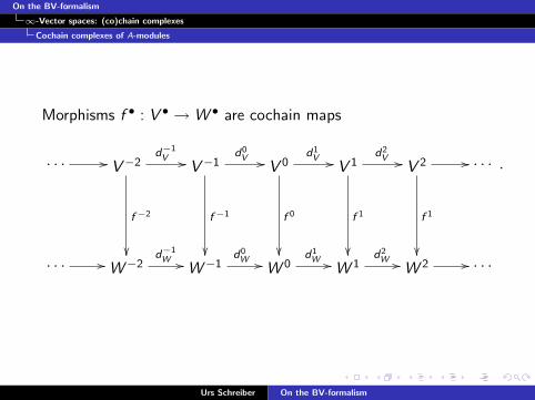
Morphisms f • : V • →W • are cochain maps
· · · // V−2d−1
V //
f −2
V−1d0
V //
f −1
V 0d1
V //
f 0
V 1d2
V //
f 1
V 2 //
f 1
· · ·
· · · // W−2d−1
W // W−1d0
W // W 0d1
W // W 1d2
W // W 2 // · · ·
.
Urs Schreiber On the BV-formalism

On the BV-formalism
∞-Vector spaces: (co)chain complexes
Cochain complexes of A-modules
We assume all chain complexes to be nontrivial only in finitelymany degrees.It is useful to distinguish the full subcategories
Ch−(A) of cochain complexes concentrated in non-positivedegree;
Ch+(A) of cochain complexes concentrated in non-negativedegree.
One may think of Ch−(A) as ω-vector spaces and of Ch+(A) asω-co-vector spaces.Using the notation
Vn := V−n
we can neatly switch back and forth between the two pictures.
Urs Schreiber On the BV-formalism
On the BV-formalism
∞-Vector spaces: (co)chain complexes
Cochain complexes of A-modules
Remark
If we forget the differentials, i.e. if we look at cochaincomplexes with all differentials trivial (the 0-maps), then theseare the same as Z-graded A-modules.
When we have nontrivial differentials, their nilpotency,d2 = 0, necessarily imposes, as discussed below, on thesegraded vector spaces the structure of supervector spaces: thesymmetric braiding is the nontrivial Z2-grading thatintroduces a sign whenever two odd-graded components areinterchanged.
Urs Schreiber On the BV-formalism

On the BV-formalism
∞-Vector spaces: (co)chain complexes
Cochain complexes of A-modules
Structure and properties and of Ch•(A).
We list some useful facts about Ch•(A).
Urs Schreiber On the BV-formalism
On the BV-formalism
∞-Vector spaces: (co)chain complexes
Cochain complexes of A-modules
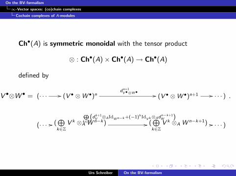
Ch•(A) is symmetric monoidal with the tensor product
⊗ : Ch•(A)× Ch•(A)→ Ch•(A)
defined by
V •⊗W • = (· · · // (V • ⊗W •)ndn+1
V•⊗W• // (V • ⊗W •)n+1 // · · · )
(· · · // (⊕k∈Z
V k ⊗A W n−k)
L
k∈Z(dk+1
V ⊗AIdWn−k +(−1)k Id
Vk⊗Adn−k+1W )
// (⊕k∈Z
V k ⊗A W n−k+1) // · · · )
.
Urs Schreiber On the BV-formalism

On the BV-formalism
∞-Vector spaces: (co)chain complexes
Cochain complexes of A-modules
Remark.
The signs appearing here are crucial. Their nature is fixed entirelyby the requirement that the tensor product is again a chaincomplex, i.e. by the requirement that (dV⊗W )2 = 0. As we will seein the following, this will also imply that our modules are subjectto the nontrivial symmetric braiding which introduces a signwhenever two odd-graded modules are interchanged. All thisfollows just from the nilpotency condition d2 = 0.One way to understand the precise nature of the signs above is tonote that when forming the tensor product V ⊗W , we obtain thedouble complex
Urs Schreiber On the BV-formalism

On the BV-formalism
∞-Vector spaces: (co)chain complexes
Cochain complexes of A-modules
...
dmW
...
dmW
· · ·
dnV // V n ⊗W m
dn+1V //
dm+1W
V n+1 ⊗W m
dm+1W
// · · ·
· · ·dn
V// V n ⊗W m+1dn+1
V //
V n+1 ⊗W m+1 //
· · ·
......
as an intermediate step. The squares commute, meaning that dV
and dW commute.
Urs Schreiber On the BV-formalism
On the BV-formalism
∞-Vector spaces: (co)chain complexes
Cochain complexes of A-modules
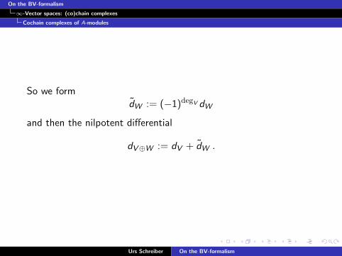
So we formdW := (−1)degV dW
and then the nilpotent differential
dV⊕W := dV + dW .
Urs Schreiber On the BV-formalism

On the BV-formalism
∞-Vector spaces: (co)chain complexes
Cochain complexes of A-modules
The tensor unit is
I • := ( · · ·d−1
I // 0d0
I // Ad1
I // 0d2
I // · · ·
· · · 0 // 00 // A
0 // 0 // · · ·
)
Urs Schreiber On the BV-formalism

On the BV-formalism
∞-Vector spaces: (co)chain complexes
Cochain complexes of A-modules
The symmetric braiding
Ch•(A)× Ch•(A)⊗ //
σ))SSSSSSSSSSSSSSS
Ch•(A)⊗ Ch•(A)
Ch•(A)× Ch•(A)
⊗
55kkkkkkkkkkkkkkkb
withσ : Ch•(A)× Ch•(A)→ Ch•(A)× Ch•(A)
Urs Schreiber On the BV-formalism

On the BV-formalism
∞-Vector spaces: (co)chain complexes
Cochain complexes of A-modules
the exchange of factors is
bnV •,W • : (
⊕k
V k ⊗A W n−k)
L
k(−1)k(n−k)
// (⊕k
W n−k ⊗A V k) .
The signs here ensure the required naturality
(⊕k
V k ⊗A W n−k)
L
k(−1)k(n−k)
//
dV⊗AId+(−1)k Id⊗AdW
(⊕k
W n−k ⊗A V k)
dW⊗AId+(−1)n−k Id⊗AdV
(⊕k
V k ⊗A W n−k+1)
L
k(−1)k(n−k+1)
// (⊕k
W n−k+1 ⊗A V k)
Urs Schreiber On the BV-formalism
On the BV-formalism
∞-Vector spaces: (co)chain complexes
Cochain complexes of A-modules
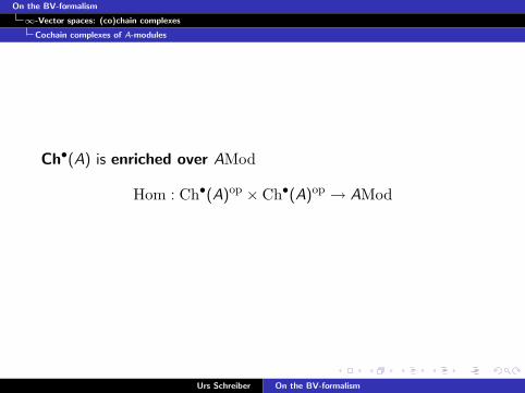
Ch•(A) is enriched over AMod
Hom : Ch•(A)op × Ch•(A)op → AMod
Urs Schreiber On the BV-formalism
On the BV-formalism
∞-Vector spaces: (co)chain complexes
Cochain complexes of A-modules
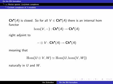
Ch•(A) is closed. So for all V ∈ Ch•(A) there is an internal homfunctor
hom(V ,−) : Ch•(A)→ Ch•(A)
right adjoint to
−⊗ V : Ch•(A)→ Ch•(A)
meaning that
Hom(U ⊗ V ,W ) ' Hom(U,hom(V ,W ))
naturally in U and W .
Urs Schreiber On the BV-formalism
On the BV-formalism
∞-Vector spaces: (co)chain complexes
Cochain complexes of A-modules
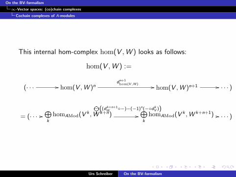
This internal hom-complex hom(V ,W ) looks as follows:
hom(V ,W ) :=
(· · · // hom(V ,W )ndn+1hom(V ,W ) // hom(V ,W )n+1 // · · · )
= (· · · //⊕k
homAMod(V k ,W k+n)
L
k((dk+n+1
W −)−(−1)n(−dkV ))
//⊕k
homAMod(V k ,W k+n+1) // · · · )
Urs Schreiber On the BV-formalism

On the BV-formalism
∞-Vector spaces: (co)chain complexes
Cochain complexes of A-modules
The differential dhom(V ,W ) here can be understood from looking atthe evaluation map
ev : hom(V ,W )⊗ V →W
which exists by general nonsense on internal homs. Letf ∈ ⊕kHom(V k ,W k+n) be any homogeneous element in theinternal hom and x ∈ V m. Write f (x) for ev(f , x). Then the factthat ev is a cochain morphism says that
dW (f (v)) = (dhom(V ,W )f )(x) + (−1)nf (dV x) .
Solving this for dhom(V ,W )f yields the action of the differential asgiven above.
Urs Schreiber On the BV-formalism
On the BV-formalism
∞-Vector spaces: (co)chain complexes
Cochain complexes of A-modules
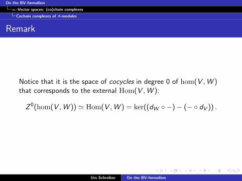
Remark
Notice that it is the space of cocycles in degree 0 of hom(V ,W )that corresponds to the external Hom(V ,W ):
Z 0(hom(V ,W )) ' Hom(V ,W ) = ker((dW −)− (− dV )) .
Urs Schreiber On the BV-formalism

On the BV-formalism
∞-Vector spaces: (co)chain complexes
Cochain complexes of A-modules
Ch•(A) has duals. Since we have a tensor unit I and an internalhom, we have duality
(·)∗ : Ch•(A)→ Ch•(A)op
given byV ∗ := hom(V , I ) .
Using the above one finds
V ∗ = (· · · // (V ∗)ndn+1
V∗ // (V ∗)n+1 // · · · )
= (· · · // (V−n)∗−(−1)n(d−n
V )∗// (V−n−1)∗ // · · · )
.
Urs Schreiber On the BV-formalism

On the BV-formalism
∞-Vector spaces: (co)chain complexes
Cochain complexes of A-modules
The unit i : I → V ⊗ V ∗ is
· · · // 0 //
0
A //
L
k
iVk
0 //
· · ·
· · · //⊕k
V k ⊗A (V k+1)∗ //⊕k
V k ⊗A (V k)∗ //⊕k
V k ⊗A (V k−1)∗ // · · ·
,
Urs Schreiber On the BV-formalism
On the BV-formalism
∞-Vector spaces: (co)chain complexes
Cochain complexes of A-modules
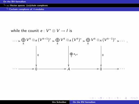
while the counit e : V ∗ ⊗ V → I is
· · · //⊕k
V k ⊗A (V k+1)∗ //
0
⊕k
V k ⊗A (V k)∗ //
L
k
eVk
⊕k
V k ⊗A (V k−1)∗ //
0
· · ·
· · · // 0 // A // 0 // · · ·
.
Urs Schreiber On the BV-formalism
On the BV-formalism
∞-Vector spaces: (co)chain complexes
Cochain complexes of A-modules
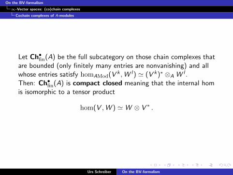
Let Ch•fin(A) be the full subcategory on those chain complexes thatare bounded (only finitely many entries are nonvanishing) and allwhose entries satisfy homAMod(V
k ,W l) ' (V k)∗ ⊗A W l .Then: Ch•fin(A) is compact closed meaning that the internal homis isomorphic to a tensor product
hom(V ,W ) 'W ⊗ V ∗ .
Urs Schreiber On the BV-formalism

On the BV-formalism
∞-Vector spaces: (co)chain complexes
Cochain complexes of A-modules
Ch•(A) has plenty of other nice structures. In particular, itnaturally is a model category.
Urs Schreiber On the BV-formalism
On the BV-formalism
∞-Vector spaces: (co)chain complexes
dg-Algebras and dg-coalgebras
dg-Algebras and dg-coalgebras
Urs Schreiber On the BV-formalism
On the BV-formalism
∞-Vector spaces: (co)chain complexes
dg-Algebras and dg-coalgebras
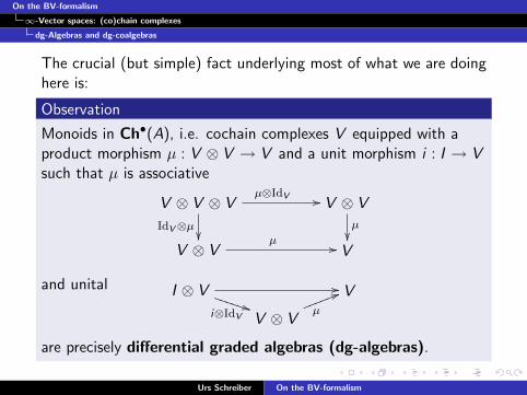
The crucial (but simple) fact underlying most of what we are doinghere is:
Observation
Monoids in Ch•(A), i.e. cochain complexes V equipped with aproduct morphism µ : V ⊗ V → V and a unit morphism i : I → Vsuch that µ is associative
V ⊗ V ⊗ Vµ⊗IdV //
IdV⊗µ
V ⊗ V
µ
V ⊗ Vµ // V
and unital I ⊗ V //
i⊗IdV**TTTTTT V
V ⊗ Vµ
55kkkkkk
are precisely differential graded algebras (dg-algebras).
Urs Schreiber On the BV-formalism
On the BV-formalism
∞-Vector spaces: (co)chain complexes
dg-Algebras and dg-coalgebras
dg-algebra
A dg-algebra is an associative graded algebra (V , ·) equipped witha graded derivation
d : V → V
of degree +1 that squares to 0,
d2 = 0 .
Urs Schreiber On the BV-formalism

On the BV-formalism
∞-Vector spaces: (co)chain complexes
dg-Algebras and dg-coalgebras
Of ocurse this has a co-version:
Defintion
Comonoids in Ch•(A), i.e. cochain complexes V equipped with acoproduct morphism δ : V → V ⊗ V and a counit morphisme : V → I such that δ is coassociative
V ⊗ V ⊗ V V ⊗ Vδ⊗IdVoo
V ⊗ V
IdV⊗δ
OO
V
δ
OO
δoo
and counital I ⊗ V oojji⊗IdV
UUUUUU V
V ⊗ Vuu
µ
kkkkkk
are precisely codifferential graded coalgebras (cdg-coalgebras).
Urs Schreiber On the BV-formalism
On the BV-formalism
∞-Vector spaces: (co)chain complexes
dg-Algebras and dg-coalgebras
cdg-coalgebra
A cdg-coalgebra is a coassociative graded coalgebra (V , ·)equipped with a graded coderivation
D : V → V
of degree +1 that squares to 0,
D2 = 0 .
Urs Schreiber On the BV-formalism
On the BV-formalism
∞-Vector spaces: (co)chain complexes
dg-Algebras and dg-coalgebras
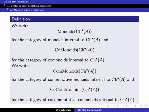
Definition
We writeMonoids(Ch•(A))
for the category of monoids internal to Ch•(A) and
CoMonoids(Ch•(A))
for the category of comonoids internal to Ch•(A).We write
ComMonoids(Ch•(A))
for the category of commutative monoids internal to Ch•(A) and
CoComMonoids(Ch•(A))
for the category of cocommutative comonoids internal to Ch•(A).
Urs Schreiber On the BV-formalism
On the BV-formalism
∞-Vector spaces: (co)chain complexes
dg-Algebras and dg-coalgebras
Quasi-free dg-(co)-algebra
Urs Schreiber On the BV-formalism

On the BV-formalism
∞-Vector spaces: (co)chain complexes
dg-Algebras and dg-coalgebras
We shall mainly be interested in dg-algebras that are free in acertain sense. These come from symmetric tensor powers.
Definition
The symmetric tensor prodct of an object V in Ch•(A) withitself is
V ∧ V := ker(IdV⊗V − bV ,V )
= im(1
2(IdV⊗V + bV ,V )) ,
where bV ,W is the component of the symmetric braiding, describedabove.Similarly the nth symmetric tensor power
∧nV
is defined by symmetrizing, using bV ,V , over all n! permutations.
Urs Schreiber On the BV-formalism

On the BV-formalism
∞-Vector spaces: (co)chain complexes
dg-Algebras and dg-coalgebras
Remark.
Notice that for chain complexes concentrated in degree 0, thesymmetric tensor product coincides with the usual symmetrictensor product of plain A-modules. For chain complexes withall differentials vanishing it corresponds to the gradedsymmetric product of the corresponding graded A-modules.
The definition of V ∧ V in terms of the image of the projector
sym :=1
2(IdV⊗V + bV ,V )
is convenient (see below), but does need to assume that weare working over a field not of characteristic 2.
Urs Schreiber On the BV-formalism
On the BV-formalism
∞-Vector spaces: (co)chain complexes
dg-Algebras and dg-coalgebras
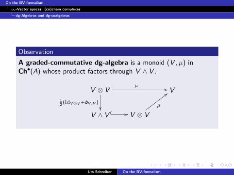
Observation
A graded-commutative dg-algebra is a monoid (V , µ) inCh•(A) whose product factors through V ∧ V .
V ⊗ Vµ //
12(IdV⊗V +bV ,V )
V
V ∧ V // V ⊗ V
µ
;;xxxxxxxxx
Urs Schreiber On the BV-formalism

On the BV-formalism
∞-Vector spaces: (co)chain complexes
dg-Algebras and dg-coalgebras
Definition
The tensor algebra over a complex V is the complex
TV :=⊕n∈N
V ⊗ · · · ⊗ V︸ ︷︷ ︸n
:= I ⊕ V ⊕ (V ⊗ V )⊕ · · · .
equipped with the tautological monoid structureThe symmetric tensor algebra over a complex V is the complex
Λ•V :=⊕n∈N∧nV = I ⊕ V ⊕ (V ∧ V )⊕ · · · .
The monoid structure · : ΛV ⊗ ΛV → ΛV on this is the one fromabove, composed with the graded symmetrization projector
µ : V ∧k ⊗ V ∧lsym // V ∧(k+l) .
Urs Schreiber On the BV-formalism
On the BV-formalism
∞-Vector spaces: (co)chain complexes
dg-Algebras and dg-coalgebras
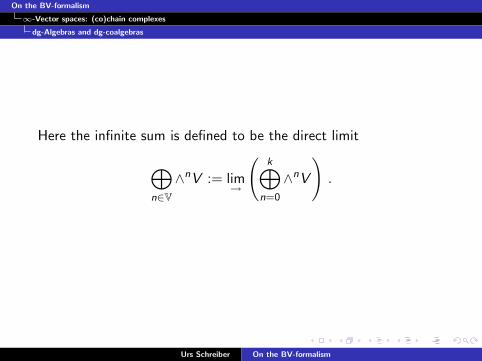
Here the infinite sum is defined to be the direct limit
⊕n∈V∧nV := lim
→
(k⊕
n=0
∧nV
).
Urs Schreiber On the BV-formalism

On the BV-formalism
∞-Vector spaces: (co)chain complexes
dg-Algebras and dg-coalgebras
Example
Let V be an ordinary vector space, regarded as a chain complexconcentrated in degree 0, with A = k the ground field. Then
TV
is the ordinary tensor algebra over V ,
ΛV
is the free symmetric tensor algebra (the bosonic Fock spaceover V ) and
Λ(V [1])
is the (free graded-commutative) Grassmann algebra over V (thefermionic Fock space over V ).
Urs Schreiber On the BV-formalism

On the BV-formalism
∞-Vector spaces: (co)chain complexes
dg-Algebras and dg-coalgebras
Example
Let (g, [·, ·]) a finite dimensional Lie algebra over our ground field.Then the Chevalley-Eilenberg algebra CE (g) of that Lie algebrais the graded commutative dg-algebra obtained by equipping
Λ(g∗[1])
with the differential
d : Λ(g∗[1])→ (Λ(g∗[1]) ∧ Λ(g∗[1]))[−1]
defined byd |g∗[1] := [·, ·]∗ .
The cohomology of the corresponding complex is, by definition, theLie algebra cohomology of g (with values in the trivial module).
Urs Schreiber On the BV-formalism

On the BV-formalism
∞-Vector spaces: (co)chain complexes
dg-Algebras and dg-coalgebras
Example
Let (g, [·, ·]) a finite dimensional Lie algebra over our ground field.Then the Weil algebra W (g) of that Lie algebra is the gradedcommutative dg-algebra obtained by equipping
Λ(g∗[1]⊕ g∗[2])
with the differential
d : Λ(g∗[1])→ (Λ(g∗[1]) ∧ Λ(g∗[1]))[−1]
defined byd |g∗[1] := [·, ·]∗ + s∗
andd(s∗(x)) := s∗dx
for all x ∈ g∗[1] and with s : g[2]→ g[1] the canonicalisomorphism. The closed elements in Λg∗[2] ⊂ Λ(g∗[1]⊕ g∗[2]) arethe symmetric invariant polynomials on g.
Urs Schreiber On the BV-formalism
On the BV-formalism
∞-Vector spaces: (co)chain complexes
dg-Algebras and dg-coalgebras
Remark
In order to put this into perspective, I make the following remark,without, at this point, trying to actually describe or explain any ofthese statements.The Weil algebra W (g) arises from CE (g) in a universal way. Allof the following are synonymous:
W (g) is the mapping cone of the identity map on CE (g). .
W (g) is the homotopy quotient of the identity map onCE (g).
W (g) is the weak cokernel of the identity map on CE (g).
Moreover
CE (g) plays the role of differential forms on G .
W (g) plays the role of differential forms on EG .
inv(g), the graded commutative algebra of closed elements inW (g)|∧g∗[2], plays the role of differential forms on BG .
Urs Schreiber On the BV-formalism

On the BV-formalism
∞-Vector spaces: (co)chain complexes
dg-Algebras and dg-coalgebras
And we have a canonical sequence
G // EG // // BG
CE (g) W (g)oooo inv(g)? _oo
Urs Schreiber On the BV-formalism
On the BV-formalism
∞-Vector spaces: (co)chain complexes
dg-Algebras and dg-coalgebras
The following fact will be of importance:
Observation
ΛV = ∧∞(I ⊕ V )
In particular
Observation
If V ∈ bfCh•(A) contains in degree 0 just the tensor unit
V 0 = A
then∧∞V
naturally is a monoid in Ch•(A).
Urs Schreiber On the BV-formalism

On the BV-formalism
Lie ∞-algebras: differential graded (co)algebra
previous: ∞-vector spaces
Lie ∞-algebras:differential graded (co)algebranext: ∞-configuration spaces
Urs Schreiber On the BV-formalism

On the BV-formalism
Lie ∞-algebras: differential graded (co)algebra
Given a graded vector space V , the tensor spaceT •(V ) :=
⊕n=0 V⊗n with V 0 being the ground field. We will
denote by T a(V ) the tensor algebra with the concatenationproduct on T •(V ):
x1 ⊗ x2 ⊗ · · · ⊗ xp
⊗xp+1 ⊗ · · · ⊗ xn 7→ x1 ⊗ x2 ⊗ · · · ⊗ xn
and by T c(V ) the tensor coalgebra with the deconcatenationproduct on T •(V ):
x1 ⊗ x2 ⊗ · · · ⊗ xn 7→∑
p+q=n
x1 ⊗ x2 ⊗ · · · ⊗ xp
⊗xp+1 ⊗ · · · ⊗ xn.
Urs Schreiber On the BV-formalism

On the BV-formalism
Lie ∞-algebras: differential graded (co)algebra
The graded symmetric algebra ∧•(V ) is the quotient of the tensoralgebra T a(V ) by the graded action of the symmetric groups Sn
on the components V⊗n. The graded symmetric coalgebra ∨•(V )is the sub-coalgebra of the tensor coalgebra T c(V ) fixed by thegraded action of the symmetric groups Sn on the components V⊗n.
Urs Schreiber On the BV-formalism
On the BV-formalism
Lie ∞-algebras: differential graded (co)algebra
Remark
∨•(V ) is spanned by graded symmetric tensors
x1 ∨ x2 ∨ · · · ∨ xp
for xi ∈ V and p ≥ 0, where we use ∨ rather than ∧ to emphasizethe coalgebra aspect, e.g.
x ∨ y = x ⊗ y ± y ⊗ x .
Urs Schreiber On the BV-formalism
On the BV-formalism
Lie ∞-algebras: differential graded (co)algebra
In characteristic zero, the graded symmetric algebra can beidentified with a sub-algebra of T a(V ) but that is unnatural andwe will try to avoid doing so. The coproduct on ∨•(V ) is given by
∆(x1∨x2 · · ·∨xn) =∑
p+q=n
∑σ∈Sh(p,q)
ε(σ)(xσ(1)∨xσ(2) · · · xσ(p))⊗(xσ(p+1)∨· · · xσ(n)) .
Urs Schreiber On the BV-formalism
On the BV-formalism
Lie ∞-algebras: differential graded (co)algebra
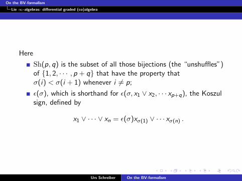
Here
Sh(p, q) is the subset of all those bijections (the “unshuffles”)of 1, 2, · · · , p + q that have the property thatσ(i) < σ(i + 1) whenever i 6= p;
ε(σ), which is shorthand for ε(σ, x1 ∨ x2, · · · xp+q), the Koszulsign, defined by
x1 ∨ · · · ∨ xn = ε(σ)xσ(1) ∨ · · · xσ(n) .
Urs Schreiber On the BV-formalism

On the BV-formalism
Lie ∞-algebras: differential graded (co)algebra
Definition (L∞-algebra)
An L∞-algebra g = (g,D) is a N+-graded vector space g equippedwith a degree -1 differential coderivation
D : ∨•g→ ∨•g
on the graded co-commutative coalgebra generated by g, such thatD2 = 0. This induces a differential
dCE(g) : Sym•(g)→ Sym•+1(g)
on graded-symmetric multilinear functions on g. When g is finitedimensional this yields a degree +1 differential
dCE(g) : ∧•g∗ → ∧•g∗
on the graded-commutative algebra generated from g∗. This is theChevalley-Eilenberg dg-algebra corresponding to the L∞-algebra g.
Urs Schreiber On the BV-formalism

On the BV-formalism
Lie ∞-algebras: differential graded (co)algebra
Remark
That the original definition of L∞-algebras in terms ofmultibrackets yields a codifferential coalgebra as above was shownin [Lada-Stasheff]. That every such codifferential comes from acollection of multibrackets this way is due to [Lada-Markl].
Urs Schreiber On the BV-formalism
On the BV-formalism
Lie ∞-algebras: differential graded (co)algebra
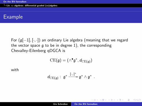
Example
For (g[−1], [·, ·]) an ordinary Lie algebra (meaning that we regardthe vector space g to be in degree 1), the correspondingChevalley-Eilenberg qDGCA is
CE(g) = (∧•g∗, dCE(g))
with
dCE(g) : g∗[·,·]∗ // g∗ ∧ g∗ .
Urs Schreiber On the BV-formalism

On the BV-formalism
Lie ∞-algebras: differential graded (co)algebra
Example
If we let ta be a basis of g and C abc the corresponding
structure constants of the Lie bracket [·, ·], and if we denote byta the corresponding basis of g∗, then we get
dCE(g)ta = −1
2C a
bctb ∧ tc .
Urs Schreiber On the BV-formalism
On the BV-formalism
Lie ∞-algebras: differential graded (co)algebra
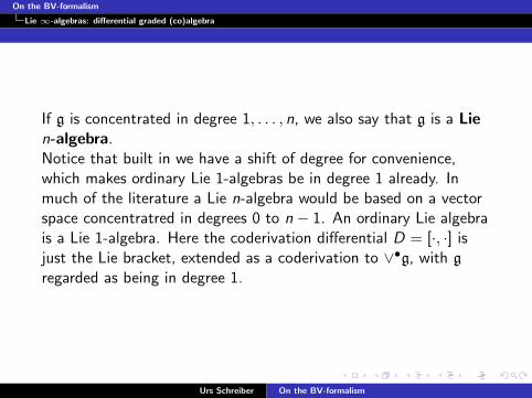
If g is concentrated in degree 1, . . . , n, we also say that g is a Lien-algebra.Notice that built in we have a shift of degree for convenience,which makes ordinary Lie 1-algebras be in degree 1 already. Inmuch of the literature a Lie n-algebra would be based on a vectorspace concentratred in degrees 0 to n − 1. An ordinary Lie algebrais a Lie 1-algebra. Here the coderivation differential D = [·, ·] isjust the Lie bracket, extended as a coderivation to ∨•g, with g
regarded as being in degree 1.
Urs Schreiber On the BV-formalism

On the BV-formalism
Lie ∞-algebras: differential graded (co)algebra
In the rest of the discussion we assume, just for simplicity andsince it is sufficient for our applications, all g to befinite-dimensional. Then, by the above, these L∞-algebras areequivalently conceived of in terms of their dual Chevalley-Eilenbergalgebras, CE(g), as indeed every quasi-free differential gradedcommutative algebra (“qDGCA”, meaning that it is free as agraded commutative algebra) corresponds to an L∞-algebra. Wewill find it convenient to work entirely in terms of qDGCAs, whichwe will usually denote as CE(g).
Urs Schreiber On the BV-formalism
On the BV-formalism
Lie ∞-algebras: differential graded (co)algebra
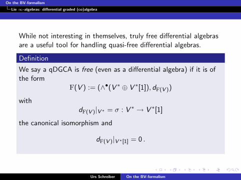
While not interesting in themselves, truly free differential algebrasare a useful tool for handling quasi-free differential algebras.
Definition
We say a qDGCA is free (even as a differential algebra) if it is ofthe form
F(V ) := (∧•(V ∗ ⊕ V ∗[1]), dF(V ))
withdF(V )|V ∗ = σ : V ∗ → V ∗[1]
the canonical isomorphism and
dF(V )|V ∗[1] = 0 .
Urs Schreiber On the BV-formalism

On the BV-formalism
Lie ∞-algebras: differential graded (co)algebra
Remark
Such algebras are indeed free in that they satisfy the universalproperty: given any linear map V →W , it uniquely extends to amorphism of qDGCAs F (V )→ (
∧•(W ∗), d) for any choice ofdifferential d .
Urs Schreiber On the BV-formalism
On the BV-formalism
Lie ∞-algebras: differential graded (co)algebra
Example
The free qDGCA on a 1-dimensional vector space in degree 0 is thegraded commutative algebra freely generated by two generators, tof degree 0 and dt of degree 1, with the differential acting asd : t 7→ dt and d : dt 7→ 0. In rational homotopy theory, thismodels the interval I = [0, 1]. The fact that the qDGCA is freecorresponds to the fact that the interval is homotopy equivalent tothe point.We will be interested in qDGCAs that arise as mapping cones ofmorphisms of L∞-algebras.
Urs Schreiber On the BV-formalism
On the BV-formalism
Lie ∞-algebras: differential graded (co)algebra
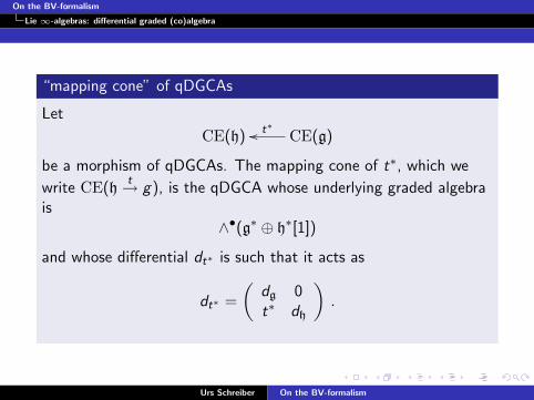
“mapping cone” of qDGCAs
Let
CE(h) CE(g)t∗oo
be a morphism of qDGCAs. The mapping cone of t∗, which we
write CE(ht→ g), is the qDGCA whose underlying graded algebra
is∧•(g∗ ⊕ h∗[1])
and whose differential dt∗ is such that it acts as
dt∗ =
(dg 0t∗ dh
).
Urs Schreiber On the BV-formalism
On the BV-formalism
Lie ∞-algebras: differential graded (co)algebra
Definition (Weil algebra of an L∞-algebra)
The mapping cone of the identity on CE(g) is the Weil algebra
W(g) := CE(gId→ g)
of g.
Urs Schreiber On the BV-formalism
On the BV-formalism
Lie ∞-algebras: differential graded (co)algebra
Proposition
For g an ordinary Lie algebra this does coincide with the ordinaryWeil algebra of g.
Urs Schreiber On the BV-formalism

On the BV-formalism
Lie ∞-algebras: differential graded (co)algebra
The Weil algebra has two important properties.
Proposition
The Weil algebra W(g) of any L∞-algebra g
is isomorphic to a free differential algebra W(g) ' F(g) , andhence is contractible;
has a canonical surjection CE(g) W(g)i∗oooo .
Urs Schreiber On the BV-formalism

On the BV-formalism
Lie ∞-algebras: differential graded (co)algebra
As a corollary we obtain
Corollary
For g any L∞-algebra, the cohomology of W(g) is trivial.
Urs Schreiber On the BV-formalism
On the BV-formalism
Lie ∞-algebras: differential graded (co)algebra
Remark
As we will shortly see, W(g) plays the role of the algebra ofdifferential forms on the universal g-bundle. The surjection
CE (g) W (g)i∗oooo plays the role of the restriction to the
differential forms on the fiber of the universal g-bundle.
Urs Schreiber On the BV-formalism

On the BV-formalism
Lie ∞-algebras: differential graded (co)algebra
Examples
We construct large families of examples the so-called String-likeextensions of L∞-algebras, based on the first two of the followingexamples and elements in L∞-algebra cohomology.
Urs Schreiber On the BV-formalism
On the BV-formalism
Lie ∞-algebras: differential graded (co)algebra
1. Ordinary Weil algebras as Lie 2-algebras
What is ordinarily called the Weil algebra W(g) of a Lie algebra(g[−1], [·, ·]) can, since it is again a DGCA, also be interpreted asthe Chevalley-Eilenberg algebra of a Lie 2-algebra. This Lie2-algebra we call inn(g). It corresponds to the Lie 2-groupINN(G ) discussed in [?]:
W(g) = CE(inn(g)) .
We haveW(g) = (∧•(g∗ ⊕ g∗[1]), dW(g)) .
Urs Schreiber On the BV-formalism
On the BV-formalism
Lie ∞-algebras: differential graded (co)algebra
1. Ordinary Weil algebras as Lie 2-algebras
Denoting by σ : g∗ → g∗[1] the canonical isomorphism, extendedas a derivation to all of W(g), we have
dW(g) : g∗[·,·]∗+σ // g∗ ∧ g∗ ⊕ g∗[1]
and
dW(g) : g∗[1]−σdCE(g)σ−1
// g∗ ⊗ g∗[1] .
Urs Schreiber On the BV-formalism
On the BV-formalism
Lie ∞-algebras: differential graded (co)algebra
1. Ordinary Weil algebras as Lie 2-algebras
With ta a basis for g∗ as above, and σta the correspondingbasis of g∗[1] we find
dW(g) : ta 7→ −1
2C a
bctb ∧ tc + σta
anddW(g) : σta 7→ −C a
bctbσtc .
Urs Schreiber On the BV-formalism
On the BV-formalism
Lie ∞-algebras: differential graded (co)algebra
1. Ordinary Weil algebras as Lie 2-algebras
The Lie 2-algebra inn(g) is, in turn, nothing but the strict Lie2-algebra as in the third example below, which comes from the
infinitesimal crossed module (gId→ g
ad→ der(g)).
Urs Schreiber On the BV-formalism

On the BV-formalism
Lie ∞-algebras: differential graded (co)algebra
2. Shifted u(1).
By the above, the qDGCA corresponding to the Lie algebra u(1) issimply
CE(u(1)) = (∧•R[1], dCE(u(1)) = 0) .
We write
CE(bn−1u(1)) = (∧•R[n], dCE(bnu(1)) = 0)
for the Chevalley-Eilenberg algebras corresponding to the Lien-algebras bn−1u(1).
Urs Schreiber On the BV-formalism
On the BV-formalism
Lie ∞-algebras: differential graded (co)algebra
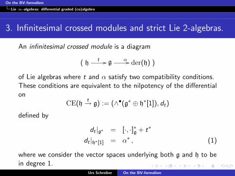
3. Infinitesimal crossed modules and strict Lie 2-algebras.
An infinitesimal crossed module is a diagram
( ht // g α // der(h) )
of Lie algebras where t and α satisfy two compatibility conditions.These conditions are equivalent to the nilpotency of the differentialon
CE(ht→ g) := (∧•(g∗ ⊕ h∗[1]), dt)
defined by
dt |g∗ = [·, ·]∗g + t∗
dt |h∗[1] = α∗ , (1)
where we consider the vector spaces underlying both g and h to bein degree 1.
Urs Schreiber On the BV-formalism

On the BV-formalism
Lie ∞-algebras: differential graded (co)algebra
3. Infinitesimal crossed modules and strict Lie 2-algebras.
Here in the last line we regard α as a linear map α : g⊗ h→ h.
The Lie 2-algebras (ht→ g) thus defined are called strict Lie
2-algebras: these are precisely those Lie 2-algebras whoseChevalley-Eilenberg differential contains at most co-binarycomponents.
Urs Schreiber On the BV-formalism
On the BV-formalism
∞-Configuration spaces: the BV-complex
previous: Lie ∞-algebras
∞-Configuration spaces:the BV-complex
Differential forms on spaces of maps
The Chevalley-Eilenberg complex.
The Koszul-Tate complex.
The full Batalin-Vilkovisky-complex.
next: Examples
Urs Schreiber On the BV-formalism

On the BV-formalism
∞-Configuration spaces: the BV-complex
Differential forms on spaces of maps
Differential forms on spaces of maps
Urs Schreiber On the BV-formalism
On the BV-formalism
∞-Configuration spaces: the BV-complex
Differential forms on spaces of maps
As mentioned in the introduction, the starting point ofBV-formalism is, in our language, the idea that we replace theconfiguration space of our system with the Lie n-algebroid whoseobjects are the configurations, and whose morphisms are the gaugetransformations.Then we need to ask: how do we obtain the configuration Lien-algebroids?The answer is: by constructing the configuration spaceinternally.
Urs Schreiber On the BV-formalism
On the BV-formalism
∞-Configuration spaces: the BV-complex
Differential forms on spaces of maps
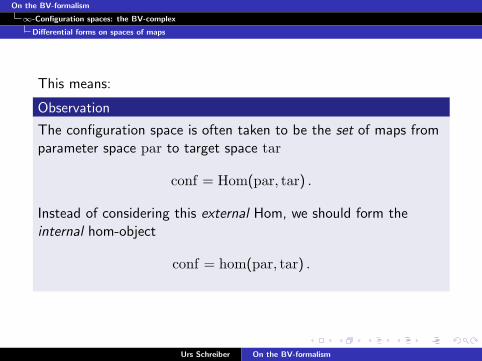
This means:
Observation
The configuration space is often taken to be the set of maps fromparameter space par to target space tar
conf = Hom(par, tar) .
Instead of considering this external Hom, we should form theinternal hom-object
conf = hom(par, tar) .
Urs Schreiber On the BV-formalism
On the BV-formalism
∞-Configuration spaces: the BV-complex
Differential forms on spaces of maps
Remark: the AKSZ approach
The observation that the BV-formalism finds its natural homewhen the configuration space is constructed internally is, more orless implicitly, due to [Alexandrov–Schwarz-Zaboronsky], reviewedby [Roytenberg].This author here, however, had his problems with extracting theabstract inner-hom construction which the component-basedformulas of these two articles could correspond to.The following construction is supposed to remedy this. Ourexamples gauge theory and higher gauge theory show that andhow this works.
Urs Schreiber On the BV-formalism

On the BV-formalism
∞-Configuration spaces: the BV-complex
Differential forms on spaces of maps
In quantum field theory, we are faced with the problem of makingsense of a diagram of the form
maps(par, tar)⊗ par
vvvvnnnnnnnnnnnnnev
''PPPPPPPPPPPPP
par tar tra // phas
in some ambient category T .We write
conf := maps(par, tar) .
The morphism tra induces the action
exp(S) : 1→ maps(conf,maps(par, tar)) .
Urs Schreiber On the BV-formalism

On the BV-formalism
∞-Configuration spaces: the BV-complex
Differential forms on spaces of maps
DGCAs of maps
We now explain and put into perspective the following definition,which is used extensively in our Examples:
Deifnition
For A and B any two DGCAs, we write
maps(B,A) := Ω•(HomDGCAs(B,A⊗ Ω•(−)))
for the DGCA of differential forms on the presheaf over manifoldswhose set of plots on any domain U is HomDGCAs(B,A⊗Ω•(U)).
Urs Schreiber On the BV-formalism
On the BV-formalism
∞-Configuration spaces: the BV-complex
Differential forms on spaces of maps
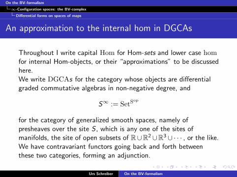
An approximation to the internal hom in DGCAs
Throughout I write capital Hom for Hom-sets and lower case homfor internal Hom-objects, or their “approximations” to be discussedhere.We write DGCAs for the category whose objects are differentialgraded commutative algebras in non-negative degree, and
S∞ := SetSop
for the category of generalized smooth spaces, namely ofpresheaves over the site S , which is any one of the sites ofmanifolds, the site of open subsets of R∪R2 ∪R3 ∪ · · · , or the like.We have contravariant functors going back and forth betweenthese two categories, forming an adjunction.
Urs Schreiber On the BV-formalism

On the BV-formalism
∞-Configuration spaces: the BV-complex
Differential forms on spaces of maps
The functorΩ•(·) : S∞ → DCGAs
acts asΩ• : X 7→ HomS∞(X ,Ω•) ,
where, in turn, here on the right Ω• denotes the smooth space ofall differential forms, given by the object in S∞ which acts as
Ω• : U 7→ Ω•(U) ,
where on the right we have the ordinary algebra of differentialforms on U.
Urs Schreiber On the BV-formalism
On the BV-formalism
∞-Configuration spaces: the BV-complex
Differential forms on spaces of maps
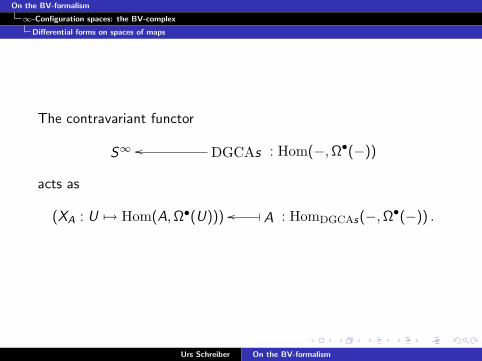
The contravariant functor
S∞ DGCAsoo : Hom(−,Ω•(−))
acts as
(XA : U 7→ Hom(A,Ω•(U))) Aoo : HomDGCAs(−,Ω•(−)) .
Urs Schreiber On the BV-formalism

On the BV-formalism
∞-Configuration spaces: the BV-complex
Differential forms on spaces of maps
Notice that S∞, being a topos, has lots of nice properties. Inparticular it is cartesian closed. The inner hom is
homS∞(X ,Y ) : U 7→ Hom(X × U,Y ) .
On the other hand, the category DGCAs doesn’t have these niceproperties in general, except after one restricts to a suitably wellbehaved subcategory. (I suspect, though, that the aboveadjunction can be turned into an equivalence on cohomology, but Iam not sure yet.)
Urs Schreiber On the BV-formalism

On the BV-formalism
∞-Configuration spaces: the BV-complex
Differential forms on spaces of maps
But we can use the above adjunction to “pull back” the inernalhom in S∞ to DGCAs, meaning that we consider
homDGCAs(−,−) :
(DGCAs)op ×DGCAsHom(−,Ω•(−))op×Hom(−,Ω•(−))op // (S∞)op × S∞
homS∞ (−,−)
S∞
Ω•
DGCAs
.
Urs Schreiber On the BV-formalism
On the BV-formalism
∞-Configuration spaces: the BV-complex
Differential forms on spaces of maps
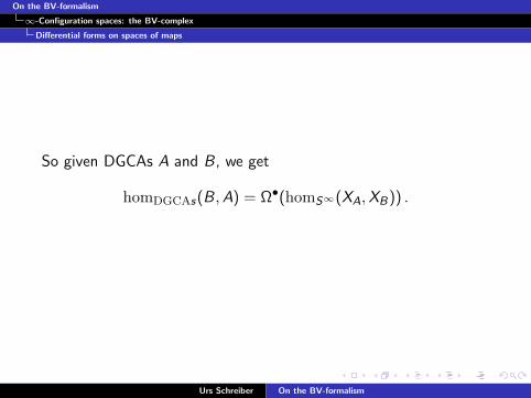
So given DGCAs A and B, we get
homDGCAs(B,A) = Ω•(homS∞(XA,XB)) .
Urs Schreiber On the BV-formalism
On the BV-formalism
∞-Configuration spaces: the BV-complex
Differential forms on spaces of maps
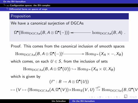
Proposition
We have a canonical surjection of DGCAs
Ω•(HomDGCAs(B,A⊗ Ω•(−))) oooo homDGCAs(B,A) .
Proof. This comes from the canonical inclusion of smooth spaces
HomDGCAs(B,A⊗ Ω•(−)) // HomS∞(XA ×−,XB)
which comes, on each U ∈ S , from the inclusion of sets
HomDGCAs(B,A⊗ Ω•(U)) → HomS∞(XA × U,XB)
which is given by(f ∗ : B → A⊗ Ω•(U))
7→ (V 7→ (HomDGCAs(A,Ω•(V ))×HomS(V ,U)f ∗→ HomDGCAs(B,Ω•(V )))) .
Urs Schreiber On the BV-formalism

On the BV-formalism
∞-Configuration spaces: the BV-complex
Differential forms on spaces of maps
Definition: currents
For A any DGCA, we say that a current on A is a smooth linearmap
c : A→ R .
For A = Ω•(X ) this reduces to the ordinary notion of currents.
Urs Schreiber On the BV-formalism

On the BV-formalism
∞-Configuration spaces: the BV-complex
Differential forms on spaces of maps
Proposition
For each element b ∈ B and current c on A, we get an element inΩ•(HomDGCAs(B,A⊗ Ω•(−))) by mapping, for each U ∈ S
HomDGCAs(B,A⊗ Ω•(U))→ Ω•(U)
f ∗ 7→ c(f ∗(b)) .
If b is in degree n and c in degree m ≤ n, then this differentialform is in degree n −m.
Urs Schreiber On the BV-formalism
On the BV-formalism
∞-Configuration spaces: the BV-complex
The Chevalley-Eilenber complex
The Chevalley-Eilenberg complex
Urs Schreiber On the BV-formalism

On the BV-formalism
∞-Configuration spaces: the BV-complex
The Koszul-Tate complex
The Koszul-Tate complex
Urs Schreiber On the BV-formalism

On the BV-formalism
∞-Configuration spaces: the BV-complex
The Koszul-Tate complex
Definition (dual Koszul complex)
Forf : M → A
a morphism of A-modules with M of rank n, let
V := (0 // V−1d0
V // V 0 // 0)
(0 // Mf // A // 0)
in Ch•(A) be the corresponding cochain complex in degree -1 and0. Then
K [f ] := ∧nV
is the (dual) Koszul complex defined by f .
Urs Schreiber On the BV-formalism

On the BV-formalism
∞-Configuration spaces: the BV-complex
The Koszul-Tate complex
Example
The crucial example of interest in the BV context is this: LetA = C (X ) for X some manifold. Let TX be the tangent bundleover X and M = Γ(TX ) its space of sections. Let S ∈ C (X ) beany function on X and set f = dS(·).
V := (0 // V−1d0
V // V 0 // 0)
(0 // Γ(TX )dS(·) // C (X ) // 0)
.
Urs Schreiber On the BV-formalism
On the BV-formalism
∞-Configuration spaces: the BV-complex
The Koszul-Tate complex
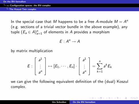
In the special case that M happens to be a free A-module M = An
(e.g. sections of a trivial vector bundle in the above example), anytuple (Ea ∈ A)na=1 of elements in A provides a morphism
E : An → A
by matrix multiplication
E :
a1
...an
7→ [E1, · · · ,En] ·
a1
...an
=n∑
k=1
akEk
we can give the following equivalent definition of the (dual) Koszulcomplex.
Urs Schreiber On the BV-formalism
On the BV-formalism
∞-Configuration spaces: the BV-complex
The Koszul-Tate complex
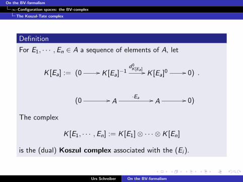
Definition
For E1, · · · ,En ∈ A a sequence of elements of A, let
K [Ea] := (0 // K [Ea]−1
d0K [Ea] // K [Ea]
0 // 0)
(0 // A·Ea // A // 0)
.
The complex
K [E1, · · · ,En] := K [E1]⊗ · · · ⊗ K [En]
is the (dual) Koszul complex associated with the (Ei ).
Urs Schreiber On the BV-formalism
On the BV-formalism
∞-Configuration spaces: the BV-complex
The Koszul-Tate complex
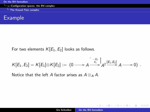
Example
For two elements K [E1,E2] looks as follows.
K [E1,E2] = K [E1]⊗K [E2] := (0 // A
−E2E1
// A2
[E1,E2] // A // 0) .
Notice that the left A factor arises as A⊗A A.
Urs Schreiber On the BV-formalism

On the BV-formalism
∞-Configuration spaces: the BV-complex
The Koszul-Tate complex
Remarks
K [E1, · · · ,En] := (· · · // A⊕n
Pna=1 ·Ek // A // 0)
The cohomology of the Koszul complex in degree 0 is thequotient
A/(E1, · · · ,En)A, .
Therefore, in the case that all other cohomology groups of theKoszul complex vanish, it provides a resolution of thisquotient. Since all A-modules appearing in the Koszulcomplex are free, this resolution is necessarily projective.
Therefore the cohomologies of the Koszul complex innon-vanishing degree measure the interdependency of the Ea.In particular, cohomology in degree -1 contains the relationsamong the Ea, namely tuples of elements v ∈ A⊕n such thatvaEa = 0 modulo the trivial relations.
Urs Schreiber On the BV-formalism
On the BV-formalism
∞-Configuration spaces: the BV-complex
The Koszul-Tate complex
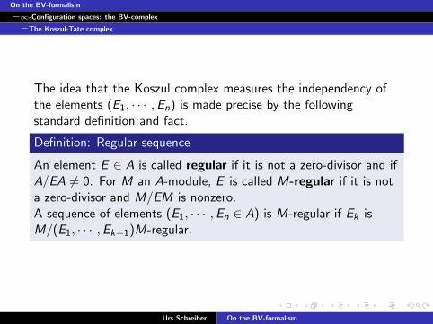
The idea that the Koszul complex measures the independency ofthe elements (E1, · · · ,En) is made precise by the followingstandard definition and fact.
Definition: Regular sequence
An element E ∈ A is called regular if it is not a zero-divisor and ifA/EA 6= 0. For M an A-module, E is called M-regular if it is nota zero-divisor and M/EM is nonzero.A sequence of elements (E1, · · · ,En ∈ A) is M-regular if Ek isM/(E1, · · · ,Ek−1)M-regular.
Urs Schreiber On the BV-formalism
On the BV-formalism
∞-Configuration spaces: the BV-complex
The Koszul-Tate complex
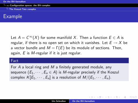
Example
Let A = C∞(X ) for some manifold X . Then a function E ∈ A isregular, if there is no open set on which it vanishes. Let E → X bea vector bundle and M = Γ(E ) be its module of sections. Then,again, E is M-regular if it is just regular.
Fact
For A a local ring and M a finitely generated module, anysequence (E1, · · · ,En ∈ A) is M-regular precisely if the Koszulcomplex K [E1, · · · ,En] is a resolution of M/(E1, · · · ,En).
Urs Schreiber On the BV-formalism

On the BV-formalism
∞-Configuration spaces: the BV-complex
The Koszul-Tate complex
If the Koszul complex K [E1, · · · ,En] is not a resolution, we canread off from its failure of acyclicity the maximal regular sequenceinside (E1, · · · ,En).
Fact
If precisely the highest r cohomology groups of K [E1, · · · ,E2]vanish, then the maximal regular sequence inside (E1, · · · ,E2) haslength r .More precisely, if
H−n+j(K [E1, · · · ,En]) = 0
for all j < r , while
H−n+r (K [E1, · · · ,En]) 6= 0
then every maximal regular sequence inside (E1, · · · ,En) haslength r .
Urs Schreiber On the BV-formalism
On the BV-formalism
∞-Configuration spaces: the BV-complex
The Koszul-Tate complex
Remark
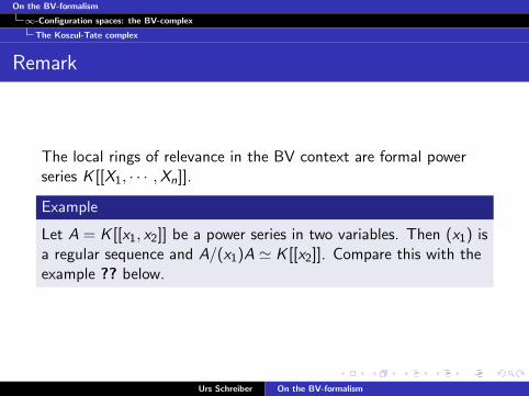
The local rings of relevance in the BV context are formal powerseries K [[X1, · · · ,Xn]].
Example
Let A = K [[x1, x2]] be a power series in two variables. Then (x1) isa regular sequence and A/(x1)A ' K [[x2]]. Compare this with theexample ?? below.
Urs Schreiber On the BV-formalism
On the BV-formalism
∞-Configuration spaces: the BV-complex
The Koszul-Tate complex
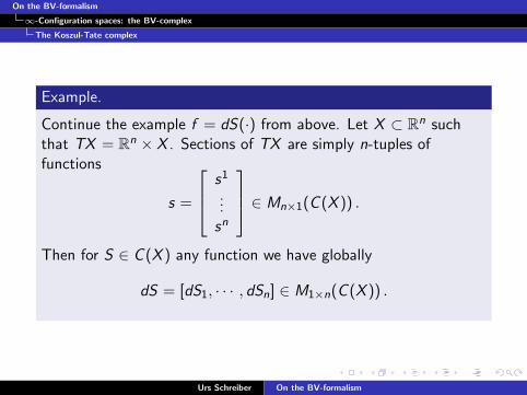
Example.
Continue the example f = dS(·) from above. Let X ⊂ Rn suchthat TX = Rn × X . Sections of TX are simply n-tuples offunctions
s =
s1
...sn
∈ Mn×1(C (X )) .
Then for S ∈ C (X ) any function we have globally
dS = [dS1, · · · , dSn] ∈ M1×n(C (X )) .
Urs Schreiber On the BV-formalism

On the BV-formalism
∞-Configuration spaces: the BV-complex
The Koszul-Tate complex
The Tate construction: killing of cohomology groups
Urs Schreiber On the BV-formalism
On the BV-formalism
∞-Configuration spaces: the BV-complex
The Koszul-Tate complex
In practice it is often useful to resolve quotients A/(E1, · · · ,En)where the (E1, · · · ,En) do not form a regular sequence.There is a canonical procedure, going back to John Tate (and usedthroughout rational homotopy theory, see the example below), tosystematically “kill” all unwanted cohomology groups byintroducing further generators.
Urs Schreiber On the BV-formalism
On the BV-formalism
∞-Configuration spaces: the BV-complex
The Koszul-Tate complex
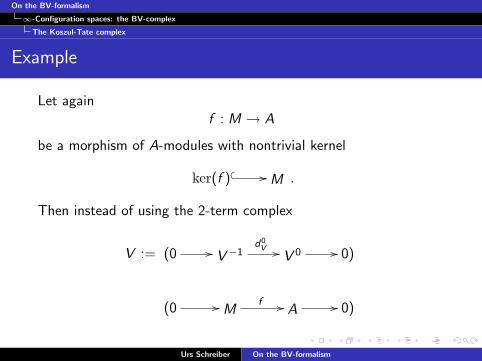
Example
Let againf : M → A
be a morphism of A-modules with nontrivial kernel
ker(f ) // M .
Then instead of using the 2-term complex
V := (0 // V−1d0
V // V 0 // 0)
(0 // Mf // A // 0)
Urs Schreiber On the BV-formalism
On the BV-formalism
∞-Configuration spaces: the BV-complex
The Koszul-Tate complex
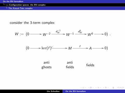
consider the 3-term complex
W := (0 // W−2d−1
W // W−1d0
W // W 0 // 0)
(0 // ker(f ) // Mf // A // 0)
antighosts
antifields
fields
.
Urs Schreiber On the BV-formalism
On the BV-formalism
∞-Configuration spaces: the BV-complex
The Koszul-Tate complex
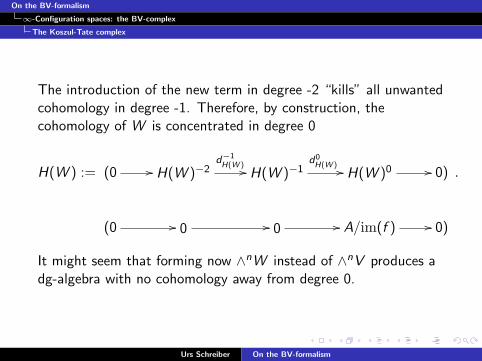
The introduction of the new term in degree -2 “kills” all unwantedcohomology in degree -1. Therefore, by construction, thecohomology of W is concentrated in degree 0
H(W ) := (0 // H(W )−2d−1
H(W ) // H(W )−1d0
H(W ) // H(W )0 // 0)
(0 // 0 // 0 // A/im(f ) // 0)
.
It might seem that forming now ∧nW instead of ∧nV produces adg-algebra with no cohomology away from degree 0.
Urs Schreiber On the BV-formalism
On the BV-formalism
∞-Configuration spaces: the BV-complex
The Koszul-Tate complex
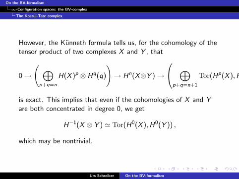
However, the Kunneth formula tells us, for the cohomology of thetensor product of two complexes X and Y , that
0→
( ⊕p+q=n
H(X )p ⊗ Hq(q)
)→ Hn(X⊗Y )→
⊕p+q=n+1
Tor(Hp(X ),Hq(Y ))
→ 0
is exact. This implies that even if the cohomologies of X and Yare both concentrated in degree 0, we get
H−1(X ⊗ Y ) ' Tor(H0(X ),H0(Y )) ,
which may be nontrivial.
Urs Schreiber On the BV-formalism
On the BV-formalism
∞-Configuration spaces: the BV-complex
The Koszul-Tate complex
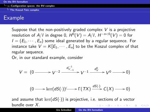
Example
Suppose that the non-positively graded complex V is a projectiveresolution of A/I in degree 0, H0(V ) = A/I , H−n<0(V ) = 0 forI = (E1, · · · ,En) some ideal generated by a regular sequence. Forinstance take V = K [E1, · · · ,En] to be the Koszul complex of thatregular sequence.Or, in our standard example, consider
V = (0 // V−2d−1
V−1 // V−1d0
V // V 0 // 0)
(0 // ker(dS(·)) // Γ(TX )dS(·) // C (X ) // 0)
and assume that ker(dS(·)) is projective, i.e. sections of a vectorbundle over X .
Urs Schreiber On the BV-formalism
On the BV-formalism
∞-Configuration spaces: the BV-complex
The Koszul-Tate complex
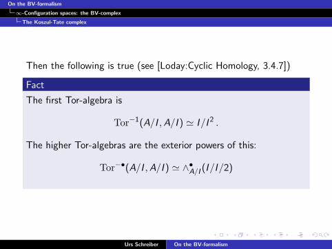
Then the following is true (see [Loday:Cyclic Homology, 3.4.7])
Fact
The first Tor-algebra is
Tor−1(A/I ,A/I ) ' I/I 2 .
The higher Tor-algebras are the exterior powers of this:
Tor−•(A/I ,A/I ) ' ∧•A/I (I/I/2)
Urs Schreiber On the BV-formalism

On the BV-formalism
∞-Configuration spaces: the BV-complex
The Koszul-Tate complex
Remark
If A = C (X ), then ∧•(I/I 2) is the algebra of differential forms onX restricted the vanishing set of (E1, · · · ,En).So we find in this case that even though the cohomology of V isconcentrated in degree 0, the cohomology of V ⊗ V can benontrivial in degree -1.
Urs Schreiber On the BV-formalism

On the BV-formalism
∞-Configuration spaces: the BV-complex
The Koszul-Tate complex
The Tate construction
Let (V , ·) be monoid in Ch•(A), hence a dg-algebra over A,concentrated in either non-positive or non-negative degree. Let usassume V is in non-positive degree for definiteness, as in ourapplications.There is a systematic way to create from (V , ·) a new dg-algebra(V ′, ·) extending it
(V ′, ·) // // (V , ·)
with the property that the cohomology of V ′ vanishes everywhereexcept in degree 0, where it coincides with the cohomology of V .
Urs Schreiber On the BV-formalism

On the BV-formalism
∞-Configuration spaces: the BV-complex
The Koszul-Tate complex
The procedure works by induction over the degree of thecohomology groups:
Let (V−k , ·) // // (V , ·) be a dg-algebra extending V suchthat
H−k<d<0(V−k) = 0 .
add an addition generator etc [need to rewrite this]
Using this procedure, one obtains the following
Fact (Tate)
For I any ideal in A there exists a free acyclic dg-algebra X suchthat H0(X ) = A/I .
In other words: we can always find some resolution of a quotientA/I by a dg-algebra.
Urs Schreiber On the BV-formalism
On the BV-formalism
∞-Configuration spaces: the BV-complex
The Koszul-Tate complex
Remark.
In the context of the BV formalism, it is for this reason that one isactually not primarily interested in Koszul complexes themselves:even if they fail to provide a resolution, using the Tate construction(“incorporating (possibly higher order)antighosts”), one alwaysforms a resolution of the “shell”.
Urs Schreiber On the BV-formalism
On the BV-formalism
∞-Configuration spaces: the BV-complex
The Koszul-Tate complex
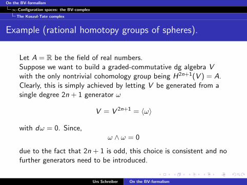
Example (rational homotopy groups of spheres).
Let A = R be the field of real numbers.Suppose we want to build a graded-commutative dg algebra Vwith the only nontrivial cohomology group being H2n+1(V ) = A.Clearly, this is simply achieved by letting V be generated from asingle degree 2n + 1 generator ω
V = V 2n+1 = 〈ω〉
with dω = 0. Since,ω ∧ ω = 0
due to the fact that 2n + 1 is odd, this choice is consistent and nofurther generators need to be introduced.
Urs Schreiber On the BV-formalism

On the BV-formalism
∞-Configuration spaces: the BV-complex
The Koszul-Tate complex
But now consider the same situation for even degree: suppose thegraded-commutative dg-algebra V has a single non-exact degree2n-generator ω with dω = 0. Then the cohomology in degree 2n isagain A. But now also all elements of the form ω ∧ ω ∧ · · ·ω arenon-vanishing and closed. In order to remove the unwantedcohomology generated by these, we throw in another generator, λ,in degree 4n − 1, and set
dλ = ω ∧ ω .
This removes all the superfluous cohomologies: now alltroublesome elements are exact.
ω ∧ ω ∧ ω ∧ · · · ∧ ω︸ ︷︷ ︸k∈N
= d(λ ∧ ω ∧ · · · ∧ ω︸ ︷︷ ︸k
) .
Urs Schreiber On the BV-formalism
On the BV-formalism
∞-Configuration spaces: the BV-complex
The Koszul-Tate complex
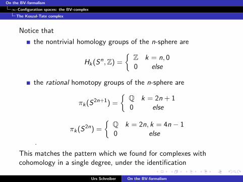
Notice that
the nontrivial homology groups of the n-sphere are
Hk(Sn, Z) =
Z k = n, 00 else
the rational homotopy groups of the n-sphere are
πk(S2n+1) =
Q k = 2n + 10 else
πk(S2n) =
Q k = 2n, k = 4n − 10 else
.
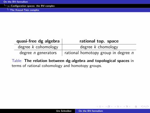
This matches the pattern which we found for complexes withcohomology in a single degree, under the identification
Urs Schreiber On the BV-formalism
On the BV-formalism
∞-Configuration spaces: the BV-complex
The Koszul-Tate complex
quasi-free dg algebra rational top. spacedegree k cohomology degree k chomology
degree n generators rational homotopy group in degree n
Table: The relation between dg-algebra and topological spaces interms of rational cohomology and homotopy groups.
Urs Schreiber On the BV-formalism
On the BV-formalism
∞-Configuration spaces: the BV-complex
The full Batalin-Vilkovisky complex
The full Batalin-Vilkoviskycomplex
Urs Schreiber On the BV-formalism

On the BV-formalism
∞-Configuration spaces: the BV-complex
The full Batalin-Vilkovisky complex
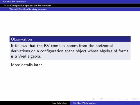
Observation
The Weil algebra W(g) of an L∞-algebra g is the same as what isaddressed as the space of functions on the shifted tangent bundleof the supermanifold on which CE(g) is the space of functions.
tangentcategory
innerautomorphism(n + 1)-group
innerderivation
Lie (n + 1)-algebra
Weil algebrashiftedtangentbundle
CE(Lie(TBG )) CE(Lie(INN(G ))) CE(inn(g)) W(g) C∞(T [1]Xg)
Figure: A remarkable coincidence of concepts relates the notion ofgraded tangency to the notion of universal bundles. See [Roberts-S.] and[Sati-S.-Stasheff].
Urs Schreiber On the BV-formalism

On the BV-formalism
∞-Configuration spaces: the BV-complex
The full Batalin-Vilkovisky complex
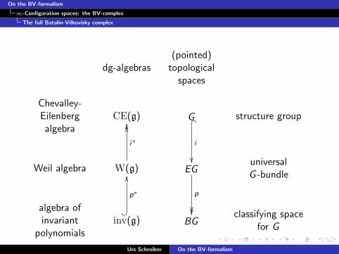
Recall from [Sati-S.-Stasheff] that the Weil algebra W(g) of anL∞-algebra g plays the role of differential forms on the universalexp(g)-bundle:
Urs Schreiber On the BV-formalism
On the BV-formalism
∞-Configuration spaces: the BV-complex
The full Batalin-Vilkovisky complex
dg-algebras(pointed)topological
spaces
Chevalley-Eilenbergalgebra
CE(g) G _
i
structure group
Weil algebra W(g)
i∗
OOOO
EG
p
universalG -bundle
algebra ofinvariant
polynomialsinv(g)
?
p∗
OO
BGclassifying space
for G
Figure: The universal G -bundle and its analog in the world ofdg-algebras.
Urs Schreiber On the BV-formalism

On the BV-formalism
∞-Configuration spaces: the BV-complex
The full Batalin-Vilkovisky complex
Definition: vertical and horizontal derivations
vertical derivations on W(g) are those vanishing on theshifted copy g∗[1] ⊂W(g)
horizontal derivations on W(g) are those vanishing on theun-shifted copy g∗ ⊂W(g)
Urs Schreiber On the BV-formalism
On the BV-formalism
∞-Configuration spaces: the BV-complex
The full Batalin-Vilkovisky complex
Observation
It follows that the BV-complex comes from the horizontalderivations on a configuration space object whose algebra of formsis a Weil algebra.
More details later.
Urs Schreiber On the BV-formalism

On the BV-formalism
Examples
previous: ∞-configuration spaces
ExamplesThe archetypical example: the (−1)-brane.
The crucial motivating example: ordinary gauge theory.
The first example showing the full power: higher gauge theory.
next: annotated literature
Urs Schreiber On the BV-formalism

On the BV-formalism
Examples
Example: the (−1)-brane
Example:the (−1)-brane
The simple – but very instructive – case where configuration spaceis finite dimensional.
Urs Schreiber On the BV-formalism

On the BV-formalism
Examples
Example: the (−1)-brane
In practice the BV complex is applied in the context of localfunctions on some jet space.But here we want to get rid of inessential technicalities as far aspossible and try to extract the pure relevant structure. For thatreason we study the BV complex in a setup where we are dealingwith ordinary functions on some manifold.Mathematically, this amounts to studying the critical points of anordinary function by cohomological means. Physically it canfruitfully be thought of as the standard BV formalism applied towhat is called a (-1)-brane: an object whose worldvolume is asingle point.
Urs Schreiber On the BV-formalism
On the BV-formalism
Examples
Example: the (−1)-brane
Remark: the algebra of functions
Some of the crucial statements about the cohomologies of thecomplexes we are about to consider depend sensitively on theprecise nature of the function algebras over which we work.For X a (real) manifold, we shall write C (X ) for an unspeifiedclass of functions on X as long as it does not matter. When itmatters, we will choose from
C (X ) ///o/o/o
Cω(X ) real analytic functionsC∞(X ) smooth functions
Urs Schreiber On the BV-formalism

On the BV-formalism
Examples
Example: the (−1)-brane
The ingredients
Definition
Let X be a smooth manifold and S ∈ C∞(X ) a smooth functionon it. Denote by Γ(TX ) the space of smooth vector fields on X .Consider the 3-term chain complex
ker(dS(·)) // Γ(TX )dS(·) // C∞(X )
−2 −1 0
with the degrees as indicated. The corresponding 3-vector spacewe denote
WC (Σ) ∈ 3Vect .
Urs Schreiber On the BV-formalism
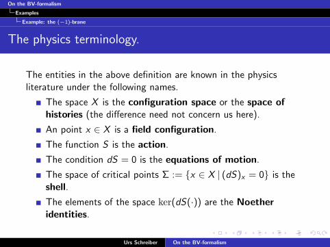
On the BV-formalism
Examples
Example: the (−1)-brane
The physics terminology.
The entities in the above definition are known in the physicsliterature under the following names.
The space X is the configuration space or the space ofhistories (the difference need not concern us here).
An point x ∈ X is a field configuration.
The function S is the action.
The condition dS = 0 is the equations of motion.
The space of critical points Σ := x ∈ X | (dS)x = 0 is theshell.
The elements of the space ker(dS(·)) are the Noetheridentities.
Urs Schreiber On the BV-formalism

On the BV-formalism
Examples
Example: the (−1)-brane
The notation WC (Σ) is for smooth functions on the “weak shell”.By construction, the cohomology of WC (Σ) is concentrated indegree 0, where it is C (X )/im(dS(·)). Following the situation inphysical examples, we assume that im(dS(·)) is the space of allsmooth functions on X that vanish on Σ. (** When is thisassumption satisfied?? **)
Observation
Hence the above chain complex is a resolution for the space ofon-shell functions, which is the way it is usually thought of.Passing from homotopical to n-categorical language this means:the 3-vector space WC (Σ) is equivalent, as a 3-vector space, tothe 1-vector space of on-shell functions.
Urs Schreiber On the BV-formalism
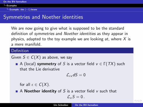
On the BV-formalism
Examples
Example: the (−1)-brane
Symmetries and Noether identities
We are now going to give what is supposed to be the standarddefinition of symmetries and Noether identities as they appear inphysics, adapted to the toy example we are looking at, where X isa mere manifold.
Definition
Given S ∈ C (X ) as above, we say
A (local) symmetry of S is a vector field v ∈ Γ(TX ) suchthat the Lie derivative
LεvdS = 0
for all ε ∈ C (X ).
A Noether identity of S is a vector field v such that
LvS = 0 .
Urs Schreiber On the BV-formalism
On the BV-formalism
Examples
Example: the (−1)-brane
Remark.
To see the connection of this definition to the definitions onemight find in most of the physics literature notice that
The above says that a local symmetry preserves the equationsof motion. This corresponds to the more commonrequirement that the local symmetry preserves the Lagrangianup to a divergence. Compare with p.7 of[KazinskiLyakhovichSharapov:1993].
To see that a Noether identity can be regarded as a vectorpreserving the action in our context, take the usual defintionand truncate jet space at 0th order everywhere. Compare with[StasheffFulpLada:2002].
In the same vein, the following plays the role of Noether’s secondtheorem in the context of our toy example.
Urs Schreiber On the BV-formalism

On the BV-formalism
Examples
Example: the (−1)-brane
Proposition: toy version of Noether’s second theorem
The space of local symmetries is isomorphic to that of Noetheridentities.
Proof. Using Cartan’s “magic formula” we have
LεvdS = εLvdS + dε ∧ v(S)
= εd(v(S)) + v(S)dε .
Clearly, every Noether identity v is hence also a local symmetry.Conversely, if v is a local symmetry then from LvdS = 0 and usingLεvdS = 0 in the above formula for all ε ∈ C (X ) it follows that vis a Noether identity.
Urs Schreiber On the BV-formalism

On the BV-formalism
Examples
Example: the (−1)-brane
chaincomplex
V = ker(dS(·)) // Γ(TX )
dS(·)// C(X )dρ // C(X ) ⊗ g∗
C(X ) ⊗ g
degree −2 −1 0 1
ass. 3-algebra _? Lie 1-algebra _?
Noether’ssecond thm.
Noetheridentities
localsymmetries
mathguys Tate Koszul
Chevalley-Eilenberg
physicsnames
antighosts antifields fields ghosts
antifieldnumber
=ω-vector
space dimension 2 1 0
ghostnumber
=ω-covector
space dimension 1
Urs Schreiber On the BV-formalism

On the BV-formalism
Examples
Example: the (−1)-brane
Local symmetry Lie algebras
We now make the assumption that we have a “Lie algebra of localgauge symmetries”.
Definition
In the case that the space of local symmetries of S is of the formC (X )⊗ g with g a finite-dimensional Lie algebra equipped with anaction ρ : g→ Γ(TX )
we say that g is the gauge Lie algebra of S and that ρ are thegauge transformations of the fields.In that case we can extend our 3-term complex WC (Σ) by themap
C (X )dρ // C (X )⊗ g∗
by setting dρ : f 7→ ρ(·)(f ) .
Urs Schreiber On the BV-formalism
On the BV-formalism
Examples
Example: the (−1)-brane
Remark
Notice that dρ is the differential of the Chevalley-Eilenbergcomplex that computes the Lie algebra cohomology of g withvalues in the Lie module C (X ) restricted to degree 0.
Urs Schreiber On the BV-formalism
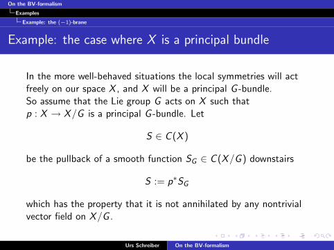
On the BV-formalism
Examples
Example: the (−1)-brane
Example: the case where X is a principal bundle
In the more well-behaved situations the local symmetries will actfreely on our space X , and X will be a principal G -bundle.So assume that the Lie group G acts on X such thatp : X → X/G is a principal G -bundle. Let
S ∈ C (X )
be the pullback of a smooth function SG ∈ C (X/G ) downstairs
S := p∗SG
which has the property that it is not annihilated by any nontrivialvector field on X/G .
Urs Schreiber On the BV-formalism

On the BV-formalism
Examples
Example: the (−1)-brane
Then the local symmetries of S are precisely the vertical vectorfields on the G -bundle X , namely sections
Γvert(TX ) := Γ(Vert(X )) ' C (X )⊗R g
of the vector bundle of vertical vector fields
Vert(X ) := ker(dp) ' P × g .
So in this case our complex is
(0 // B−2 // B−1 // C (X ) // A⊗ g // 0)
(0 // Γvert(TX ) // Γ(TX )dS(·) // C (X )
dρ // C (X )⊗R g // 0)
.
Urs Schreiber On the BV-formalism

On the BV-formalism
Examples
Example: the (−1)-brane
invariant functions on the trivial circle bundle
As a simple special case, consider the following example, whichmodels essentially the harmonic oscillator with a circle worth ofgauge degeneracies thrown in:Let
X = R× S1
the cylinder, thought of as the trivial circle bundle
p : X → R
and let the action S ∈ Cω(X ) be
S = p∗(x 7→ x2) .
Thenker(dS) = ker(dp)
are the analytic vertical vector fields on S1.Urs Schreiber On the BV-formalism

On the BV-formalism
Examples
Example: the (−1)-brane
Since dS is just multiplication of (component) functions by x , wefind that the on-shell functions are indeed precisely the quotient
Cω(Σ) ' coker(dS(·)) = Cω(X )/im(dS(·)) .
Since furthermoreker(dρ) ' Cω(X/G )
we find that the cohomology of the above complex in degree 0 isprecisely that of gauge-invariant on-shell functions
Cω(Σ/G ) = Cω(0) = R .
Urs Schreiber On the BV-formalism

On the BV-formalism
Examples
Example: ordinary gauge theory
Example:ordinary gauge theory
The case where configuration space is the space of Lie-algebravalued forms on some manifold.
Urs Schreiber On the BV-formalism
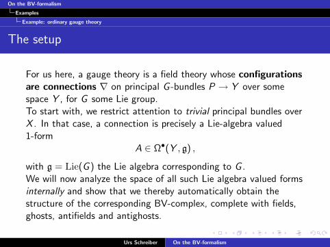
On the BV-formalism
Examples
Example: ordinary gauge theory
The setup
For us here, a gauge theory is a field theory whose configurationsare connections ∇ on principal G -bundles P → Y over somespace Y , for G some Lie group.To start with, we restrict attention to trivial principal bundles overX . In that case, a connection is precisely a Lie-algebra valued1-form
A ∈ Ω•(Y , g) ,
with g = Lie(G ) the Lie algebra corresponding to G .We will now analyze the space of all such Lie algebra valued formsinternally and show that we thereby automatically obtain thestructure of the corresponding BV-complex, complete with fields,ghosts, antifields and antighosts.
Urs Schreiber On the BV-formalism

On the BV-formalism
Examples
Example: ordinary gauge theory
Let g be any (finite dimensional) Lie ∞-algebra, CE(g) itsChevalley-Eilenberg DGC algebra and W(g) its Weil DGCA.For Y any smooth space, g-valued differential forms on Y areDGCA morphisms
Ω•(Y ) W(g)(A,FA)oo .
So the set of g-valued differential forms is
HomDGCAs(W(g),Ω•(Y )) .
Urs Schreiber On the BV-formalism

On the BV-formalism
Examples
Example: ordinary gauge theory
We want to consider the algebra of differential forms on thesmooth space of g-valued forms on Y :
maps(W(g),Ω•(Y ))
according to Differential forms on spaces of maps.
Urs Schreiber On the BV-formalism
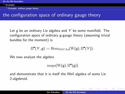
On the BV-formalism
Examples
Example: ordinary gauge theory
the configuration space of ordinary gauge theory
Let g be an ordinary Lie algebra and Y be some manifold. Theconfiguration space of ordinary g-gauge theory (assuming trivialbundles for the moment) is
Ω•(Y , g) := HomDGCAs(W(g),Ω•(Y )) .
We now analyze the algebra
maps(W(g),Ω•(g))
and demonstrate that it is itself the Weil algebra of some Lie2-algebroid.
Urs Schreiber On the BV-formalism

On the BV-formalism
Examples
Example: ordinary gauge theory
To make contact with the physics literature and most of theBV-literature, we describe everything in components.So let Y = Rn and let xµ be the canonical set of coordinatefunctions on Y . Choose a basis ta of g and let ta be thecorresponding dual basis of g∗. Denote by
δy ι ∂∂xµ
the delta-current on Ω•(Y ) which sends a 1-form ω to
ωµ(y) := ω(∂
∂xµ)(y) .
Urs Schreiber On the BV-formalism
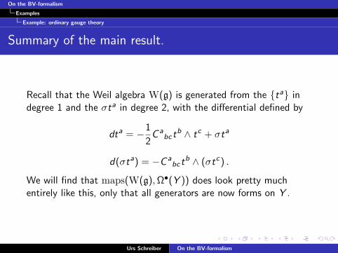
On the BV-formalism
Examples
Example: ordinary gauge theory
Summary of the main result.
Recall that the Weil algebra W(g) is generated from the ta indegree 1 and the σta in degree 2, with the differential defined by
dta = −1
2C a
bctb ∧ tc + σta
d(σta) = −C abct
b ∧ (σtc) .
We will find that maps(W(g),Ω•(Y )) does look pretty muchentirely like this, only that all generators are now forms on Y .
Urs Schreiber On the BV-formalism

On the BV-formalism
Examples
Example: ordinary gauge theory
fieldsn
Aaµ(y), (FA)µν (y) ∈ Ω0(Ω(Y , g)) | y ∈ Y , µ, ν ∈ 1, · · · , dim(Y ), a ∈ 1, . . . , dim(g)
o
ghostsn
ca(y)Ω1(Ω(Y , g)) | y ∈ Y , a ∈ 1, . . . , dim(g)o
antifields
∂
∂δAaµ(y)
∈ Hom(Ω1(Ω(Y , g)), R) | y ∈ Y , µ ∈ 1, · · · , dim(Y ), a ∈ 1, . . . , dim(g)
anti-ghostsn
∂∂βa(y)
∈ Hom(Ω2(Ω(Y , g)), R) | y ∈ Y , dim(Y ), a ∈ 1, . . . , dim(g)o
Table: The BV field content of gauge theory obtained from ouralmost internal hom of dg-algebras, definition ??. The dgc-algebramaps(W(g),Ω•(Y )) is the algebra of differential forms on a smoothspace of maps from Y to the smooth space underlying W(g). In theabove table β is a certain 2-form that one finds in this algebra of formson the space of g-valued forms.
Urs Schreiber On the BV-formalism

On the BV-formalism
Examples
Example: ordinary gauge theory
Remark.
Before looking at the details of the computation, recall that ann-form ω in maps(W(g),Ω•(Y )) is an assignment
U
φ
HomDGCAs(W(g),Ω•(Y × U))ωU // Ω•(U)
V HomDGCAs(W(g),Ω•(Y × V ))ωV //
φ∗
OO
Ω•(V )
φ∗
OO
of forms on U to g-valued forms on Y × U for all manifolds U,conatural in U.We concentrate on those n-forms ω which arise in the way ofproposition ??.
Urs Schreiber On the BV-formalism
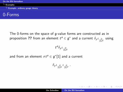
On the BV-formalism
Examples
Example: ordinary gauge theory
0-Forms
The 0-forms on the space of g-value forms are constructed as inproposition ?? from an element ta ∈ g∗ and a current δy ι ∂
∂xµusing
taδy ι ∂∂xµ
and from an element σta ∈ g∗[1] and a current
δy ι ∂∂xµ
ι ∂∂xν
.
Urs Schreiber On the BV-formalism
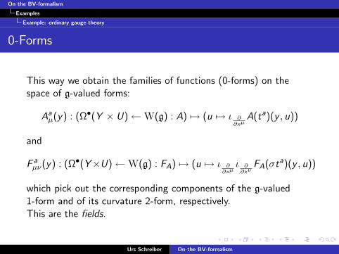
On the BV-formalism
Examples
Example: ordinary gauge theory
0-Forms
This way we obtain the families of functions (0-forms) on thespace of g-valued forms:
Aaµ(y) : (Ω•(Y × U)←W(g) : A) 7→ (u 7→ ι ∂
∂xµA(ta)(y , u))
and
F aµν(y) : (Ω•(Y×U)←W(g) : FA) 7→ (u 7→ ι ∂
∂xµι ∂
∂xνFA(σta)(y , u))
which pick out the corresponding components of the g-valued1-form and of its curvature 2-form, respectively.This are the fields.
Urs Schreiber On the BV-formalism
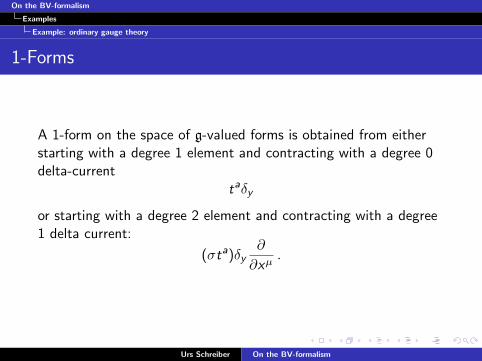
On the BV-formalism
Examples
Example: ordinary gauge theory
1-Forms
A 1-form on the space of g-valued forms is obtained from eitherstarting with a degree 1 element and contracting with a degree 0delta-current
taδy
or starting with a degree 2 element and contracting with a degree1 delta current:
(σta)δy∂
∂xµ.
Urs Schreiber On the BV-formalism
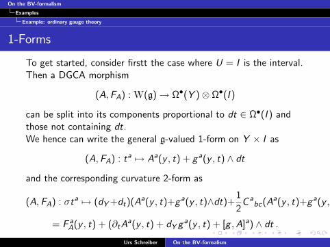
On the BV-formalism
Examples
Example: ordinary gauge theory
1-Forms
To get started, consider firstt the case where U = I is the interval.Then a DGCA morphism
(A,FA) : W(g)→ Ω•(Y )⊗ Ω•(I )
can be split into its components proportional to dt ∈ Ω•(I ) andthose not containing dt.We hence can write the general g-valued 1-form on Y × I as
(A,FA) : ta 7→ Aa(y , t) + ga(y , t) ∧ dt
and the corresponding curvature 2-form as
(A,FA) : σta 7→ (dY +dt)(Aa(y , t)+ga(y , t)∧dt)+
1
2C a
bc(Aa(y , t)+ga(y , t)∧dt)∧(Ab(y , t)+gb(y , t)∧dt)
= F aA(y , t) + (∂tA
a(y , t) + dY ga(y , t) + [g ,A]a) ∧ dt .
Urs Schreiber On the BV-formalism
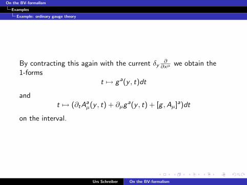
On the BV-formalism
Examples
Example: ordinary gauge theory
By contracting this again with the current δy∂
∂xµ we obtain the1-forms
t 7→ ga(y , t)dt
andt 7→ (∂tA
aµ(y , t) + ∂µga(y , t) + [g ,Aµ]a)dt
on the interval.
Urs Schreiber On the BV-formalism

On the BV-formalism
Examples
Example: ordinary gauge theory
1-Forms
We will identify the first one with the component of the 1-forms onthe space of g-valued forms on Y called the ghosts and the secondone with the 1-forms which are killed by the derivations called theanti-fields.To see more of this structure, consider now U = I 2, the unitsquare.Then a DGCA morphism
(A,FA) : W(g)→ Ω•(Y )⊗ Ω•(I 2)
can be split into its components proportional to dt1, dt2 ∈ Ω•(I 2).
Urs Schreiber On the BV-formalism

On the BV-formalism
Examples
Example: ordinary gauge theory
1-Forms
We hence can write the general g-valued 1-form on Y × I as
(A,FA) : ta 7→ Aa(y , t) + gai (y , t) ∧ dt i ,
and the corresponding curvature 2-form as
(A,FA) : σta 7→ (dY +dI 2)(Aa(y , t)+gai (y , t)∧dt i+ha(y , t)dt1∧dt2)
+1
2C a
bc(Aa(y , t)+ga
i (y , t)∧dt i+ha(y , t)dt1∧dt2)∧(Ab(y , t)+gbi (y , t)∧dt i )
= F aA(y , t) + (∂t i Aa(y , t) + dY ga
i (y , t) + [gi ,A]a) ∧ dt i
+(∂igaj + [gi , gj ]
a)dt i ∧ dt j .
Urs Schreiber On the BV-formalism

On the BV-formalism
Examples
Example: ordinary gauge theory
1-Forms
By contracting this again with the current δy∂
∂xµ we obtain the1-forms
t 7→ gai (y , t)dt i
andt 7→ (∂tA
aµ(y , t) + ∂µga
i (y , t) + [gi ,Aµ]a)dt i
on the unit square.This are again the local values of our
ca(y) ∈ Ω1(Ω•(Y , g))
andδAa
µ(Y ) ∈ Ω1(Ω•(Y , g)) .
Urs Schreiber On the BV-formalism
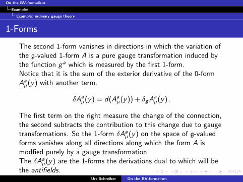
On the BV-formalism
Examples
Example: ordinary gauge theory
1-Forms
The second 1-form vanishes in directions in which the variation ofthe g-valued 1-form A is a pure gauge transformation induced bythe function ga which is measured by the first 1-form.Notice that it is the sum of the exterior derivative of the 0-formAa
µ(y) with another term.
δAaµ(y) = d(Aa
µ(y)) + δgAaµ(y) .
The first term on the right measure the change of the connection,the second subtracts the contribution to this change due to gaugetransformations. So the 1-form δAa
µ(y) on the space of g-valuedforms vanishes along all directions along which the form A ismodfied purely by a gauge transformation.The δAa
µ(y) are the 1-forms the derivations dual to which will bethe antifields.
Urs Schreiber On the BV-formalism

On the BV-formalism
Examples
Example: ordinary gauge theory
2-Forms
We have already seen the 2-form appear on the standard square.We call this 2-form
βa ∈ Ω2(Ω•(Y , g)) ,
corresponding on the unit square to the assignment
βa : (Ω•(Y × I 2)←W(g) : A) 7→ (∂igaj + [gi , gj ]
a)dt i ∧ dt j .
There is also a 2-form in the game, coming from (σta)δy .Then one immediately sees that our forms on the space of g-valuedforms satisfy the relations
dca(y) = −1
2C a
bccb(y) ∧ cc(y) + βa(y)
anddβa(y) = −C a
bcca(y) ∧ cb(y) .
Urs Schreiber On the BV-formalism
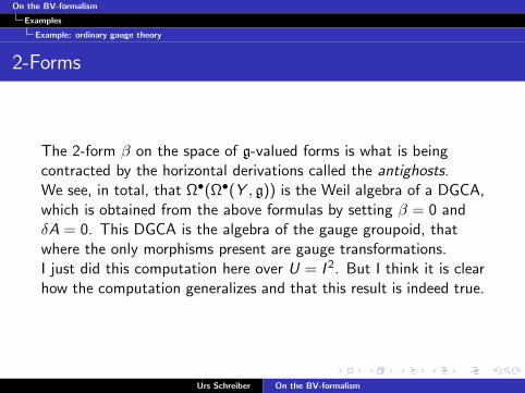
On the BV-formalism
Examples
Example: ordinary gauge theory
2-Forms
The 2-form β on the space of g-valued forms is what is beingcontracted by the horizontal derivations called the antighosts.We see, in total, that Ω•(Ω•(Y , g)) is the Weil algebra of a DGCA,which is obtained from the above formulas by setting β = 0 andδA = 0. This DGCA is the algebra of the gauge groupoid, thatwhere the only morphisms present are gauge transformations.I just did this computation here over U = I 2. But I think it is clearhow the computation generalizes and that this result is indeed true.
Urs Schreiber On the BV-formalism

On the BV-formalism
Examples
Example: higher gauge theory
Example:higher gauge theory
The case where configuration space is the space of Lie ∞-algebravalued forms on some manifold.
Urs Schreiber On the BV-formalism
On the BV-formalism
Examples
Example: higher gauge theory
A field configuration of a higher gauge theory is a connection of aprincipal G(n) n-bundle, for G(n) some Lie n-group. The mostfamiliar example is the structure 2-group G(n) = G(2) = BU(1)which yields abelian gerbes.As before, we start by concentrating on the case that the n-bundlein question is actually trivial. In that case a connection is preciselya differential form datum with values in the Lie n-algebrag := Lie(G(n)), as described in [Sati-S.-Stasheff].
Urs Schreiber On the BV-formalism

On the BV-formalism
Examples
Example: higher gauge theory
So the discussion is completely analogously to the exampleOrdinary gauge theory, only that we use the Weil algebra W(g) ofthe Lie ∞-algebra g wherever we had used before the Weil algebraof an ordinary Lie algebra.
Urs Schreiber On the BV-formalism

On the BV-formalism
Examples
Example: higher gauge theory
For a Lie n-algebra we find k-fold ghosts-of-ghosts and theircorresponding antifields for 1 ≤ k ≤ n.The configuration space of a higher gauge theory with structureLie n-algebra g is a Lie n-groupoid. See also [Baez-S., S.-Waldorf].
Urs Schreiber On the BV-formalism
On the BV-formalism
Annotated literature
previous: Examples
Annotated literatureA completely incomplete and highly subjective selection of somebackground literature, together with some remarks.
Urs Schreiber On the BV-formalism
On the BV-formalism
Annotated literature
Glenn BarnichAlgebraic structure of gauge systems: Theory and Applicationspdf slides for a talk at Bedlewo, October 19, 2007 available athttp://homepages.ulb.ac.be/ gbarnich/bedlewo.pdf
This is one of the better physics-style overviews ofBV-formalism in quantum field theory. The items on slidenumber 3 correspond to our example The (-1)-brane.
Urs Schreiber On the BV-formalism
On the BV-formalism
Annotated literature
Mathematical insight into BV-formalism
Jim StasheffThe (secret?) homological algebra of the Balalin-Vilkoviskyapproach[http://arxiv.org/abs/hep-th/9712157]
In this article the well-known homological algebraic structuresunderlying the BV-formalism are explicitly pointed out, moreor less for the first time apparently. The Chevalley-Eilenbergcomplex and the Koszul-Tate complex sitting inside theBV-complex are pointed out, and the relation to L∞-algebra,which I mentioned in Lie ∞-algebras, is mentioned.Follow the references given there.
Urs Schreiber On the BV-formalism

On the BV-formalism
Annotated literature
Conceptual insights on the BV-formalism
The following three articles on BV-formalism stand out in thatthey indicate a deeper meaning underlying the formalism, which wediscuss in Differential forms on spaces of maps:
Urs Schreiber On the BV-formalism
On the BV-formalism
Annotated literature
Conceptual insights into the BV-formalism
Alexandrov, Kontsevich, Schwarz and ZaboronskyThe Geometry of the Master Equation and TopologicalQuantum Field Theory[http://arxiv.org/refs/hep-th/0608150]
Reviewed in
D. RoytenbergAKSZ-BV Formalism and Courant Algebroid-inducedTopological Field Theories[http://arxiv.org/abs/hep-th/0608150]
This develops the idea that configuration space conf has to beformed as something close to the internal hom in dg-algebras.See Differential forms on spaces of maps.
Urs Schreiber On the BV-formalism
On the BV-formalism
Annotated literature
Conceptual insights into the BV-formalism
E. WittenA note on the antibracket formalismModern Physics Letters A, 5 7, 487-494
This shows that the BV-Laplacian is nothing but the exteriordifferential acting on a non-standard Clifford module.
Urs Schreiber On the BV-formalism
On the BV-formalism
Annotated literature
The following references are to the articles which the discussion ofgauge theory makes use of and the discussion ofhigher gauge theory relies on.
Urs Schreiber On the BV-formalism

On the BV-formalism
Annotated literature
Aspects of higher gauge theory
J. Baez and U. S.Higher Gauge theoryin Contemporary Mathematics, 431,Categories in Algebra, Geometry and Mathematical Physicsavailable as [arXiv:math/0511710]
This article discusses the parallel transport of Lie 2-algebravalued connections for possibly nontrivial 2-bundles. In thespecial case the the Lie 2-group is an automorphism 2-group,the differential 2-cocycles thus obtained reproduce those fornonabeliam gerbes with connection.
Urs Schreiber On the BV-formalism

On the BV-formalism
Annotated literature
Aspects of higher gauge theory
D. Roberts and U. S.The inner automorphism 3-group of a strict 2-group[arXiv:0708.1741]
This article describes the Lie 3-group obtained from
integrating the Lie 3-algebra inn(ht→ g) for (h
t→ g) a strictLie 2-algebra. Notice that
W(ht→ g) = CE(inn(h
t→ g)) .
The article closes by indicating in which sense the innerautomorphism 3-group is the univseral 2-bundle of thecorresponding strict 2-group. This is the integrated analog of
the fact we use here: that W(ht→ g) plays the role of forms
on the universal exp(ht→ g)2-bundle.
Urs Schreiber On the BV-formalism

On the BV-formalism
Annotated literature
Aspects of higher gauge theory
H. Sati, U. S. and J. StasheffLie ∞-algebra connections and application to String- andChern-Simons n-transport[http://www.math.uni-hamburg.de/home/schreiber/LCon.pdf]
This article describes a way to handle Lie ∞-algebrag-connections entirely at the level of Lie ∞-algebras. Thenotion of Lie ∞-algebra valued forms used here, as well as thecrucial interpretation of W(g) as forms on the universalexp(g)-bundle is discussed there.
Urs Schreiber On the BV-formalism
On the BV-formalism
Annotated literature
Aspects of higher gauge theory
U. S. and K. WaldorfThe geometry of smooth 2-functors
U.S. and K. WaldorfParallel transport and 2-functors
Urs Schreiber On the BV-formalism