on the chance of freak waves at sea - citeseer

J. Fluid Mech. (1998), ol. 355, pp. 113–138. Printed in the United Kingdom

# 1998 Cambridge University Press

113

On the chance of freak waves at sea

By BENJAMIN S. WHITE1 BENGT FORNBERG2

"Exxon Research and Engineering Co., Route 22 East, Annandale, NJ 08801, USA

#Department of Applied Mathematics, University of Colorado at Boulder, Campus Box 526,Boulder, CO 80309-0526, USA

(Received 28 October 1996 and in revised form 4 July 1997)

When deep-water surface gravity waves traverse an area with a curved or otherwisevariable current, the current can act analogously to an optical lens, to focus waveaction into a caustic region. In this region, waves of surprisingly large size, alternativelycalled freak, rogue, or giant waves are produced. We show how this mechanismproduces freak waves at random locations when ocean swell traverses an area ofrandom current. When the current has a constant (possibly zero) mean with smallrandom fluctuations, we show that the probability distribution for the formation of afreak wave is universal, that is, it does not depend on the statistics of the current, butonly on a single distance scale parameter, provided that this parameter is finite andnon-zero. Our numerical simulations show excellent agreement with the theory, evenfor current standard deviation as large as 1.0 m s−". Since many of these results arederived for arbitrary dispersion relations with certain general properties, they includeas a special case previously published work on caustics in geometrical optics.

1. Introduction

Waves of surprisingly large size, alternatively called freak, rogue, or giant waves, area well-documented hazard to mariners. Perhaps the most celebrated incident occurredduring the world’s first solo circumnavigation, when, in 1896, well off the Patagoniancoast, the Spray’s hull was completely submerged by a giant wave as Captain JoshuaSlocum (1899) clung to the peak halyards. Captain Mallory (1974) analysed elevenmore-recent incidents, off the south-east coast of South Africa, of freak waves whichcaused damage to large vessels, including one ship which was cleaved in half. All theseoccurrences were in an area renowned for producing freak waves when a large oceanswell opposes the swift Agulhas current.

Peregrine (1976) suggested that, in areas of strong current such as the Agulhas,abnormally large waves could be produced when wave action is concentrated byrefraction into a caustic region. In this scenario, a curved or otherwise variable currentacts analogously to an optical lens to focus wave action. Gerber (1996) applied thisidea, and the theory of Gerber (1993), to explain the large waves encountered in theAgulhas current, examining in particular the 1986 incident involving the semi-submersible Actinia. A related theory was given by Gutshabash & Lavrenov (1986).Irvine & Tilley (1988) analysed Synthetic Aperture Radar (SAR) data of the Agulhascurrent, and concluded that caustics caused by meanders in the Agulhas could producegiant waves.

Further support for the caustic theory of giant waves is given by Smith (1976), whocalculated the shape of a wave near a caustic, and produced an asymmetry, as is

114 B. S. White and B. Fornberg

reported by mariners. Mallory (1974) describes freak waves as having a steeper forwardface preceded by a deep trough, or ‘hole in the sea’.

We adopt here the nomenclature of Bacon (1991, in the classic text of Coles), todistinguish between extreme waves, representing the tail of some typical statisticaldistribution of wave heights (generally a Rayleigh distribution), and freaks, ‘defined aswaves of a height occurring more often than would be expected from the ‘‘background’’probability distribution’. Note however that not all authorities accept this distinction,e.g. Van Dorn (1993). Although Sand et al. (1990), in their analysis of waves on theDanish Continental Shelf, do not use this nomenclature, they do confirm the existenceof large waves that Bacon would call freak, rather than extreme. These waves, in theirwords, ‘do not belong to the traditional short term statistical distributions used forocean waves. The waves are too high, too asymmetric and too steep.’

The expected structure of extreme waves was calculated theoretically by Phillips, Gu& Donelan (1993a), who obtained good agreement with data, as did Phillips, Gu &Walsh (1993b). In contrast to Smith’s (1976) analysis of giant waves, this expectedstructure of extreme waves is symmetric. A more definitive mathematical theoryapplicable to determining the structure of extreme waves is given by Lindgren (1970).

In this paper, we compute the probability distribution for the formation of a freakwave when a regular ocean swell traverses a region of deep water with random currentfluctuations. It is assumed that freak waves are produced by caustics resulting from rayfocusing when the swell interacts with the random current. Under wide hypotheses,when the mean current is constant (possibly zero) and the random current fluctuationsare small, the probability distribution for the formation of a freak is universal, i.e. itdoes not depend on the details of the current distribution, but is described by auniversal mathematical form controlled by a single distance scale parameter, providedthat this parameter is finite and non-zero. The theory is verified with Monte Carlosimulations, and good agreement is obtained, even when the standard deviation of thecurrent is as large as 1 m s−". Since many of the main results are derived for arbitraryray systems generated by two-dimensional dispersion relations, they include, forexample, previously published results on caustics in geometrical optics.

Note that in this model caustics occupy a fixed position in space near which freakwaves are generated. Conditions like this were encountered by the ketch Tzu Hangwhen she was pitchpoled in the South Pacific, 900 miles offshore, in the first of her twounsuccessful attempts to round Cape Horn (Smeeton 1959). Henderson (1991)postulated the existence of uncharted seamounts to explain crew member JohnGuzzwell’s description of the sea state as similar to ‘what would be encountered witha long swell passing over a shoal area’. A caustic region is an alternative explanation.Peregrine (1976) suggested that a better description of wave behaviour in a causticregion might be given by considering the behaviour of a short wave group, that, hesurmised, might ‘show just one or two large waves persisting for a limited time’.

To study the focusing of waves, we introduce, in §2, the ray theory for water waves(Longuet-Higgins & Stewart 1961; Whitham 1974; Peregrine 1976), in which wave raysare refracted by a spatially varying current. In this theory, a singularity in the ray fielddevelops when two rays, which are initially (infinitesimally) close, coalesce. A causticis the locus of such points, where rays are pinched together, and large amplitudesoccur. In numerical simulations, the location of a caustic may be detected bymonitoring the ‘Jacobian’, or equivalently the ‘raytube area’, which is the distancebetween two initially close rays, normalized by their initial separation. A caustic is thendetermined as the locus of points in space where the raytube area vanishes.

In §2 we also derive new equations for the propagation of raytube area (or,

On the chance of freak waes at sea 115

equivalently, the Jacobian) along a ray. This is a new development in the ray theoryfor water waves, with many possible applications beyond that of determining thelocation of caustics, for which these equations are utilized here. In the assessment ofIrvine & Tilley (1988), the Jacobian ‘ is the most important factor governing energydensity in situations dominated by refraction’. Furthermore, we derive these equationsin great generality, for arbitrary dispersion relations in two dimensions, so that they arealso applicable to a wide range of wave propagation problems other than those ofsurface gravity waves in deep water. In this way, our equations can be seen as ageneralization of the raytube area equations that are known for non-dispersive waves(see, e.g. Kulkarny & White 1982).

The principle of conservation of wave action (CWA) (Longuet-Higgins & Stewart1961; Whitham 1974; Peregrine 1976) may be used, in conjunction with ray theory, todetermine wave amplitudes at points in space that are not near a caustic. Forcompleteness, and to demonstrate the amplitude singularity at a caustic, we use CWAin §2 to express the wave amplitude in terms of the raytube area. However, all otherresults in this paper, including the raytube area equations and the universal rogueprobability curve, are independent of the assumption of CWA. This point is importantbecause CWA has, in general, only been demonstrated mathematically for irrotationalcurrents and we intend to apply our results for example to random eddy fields withvarious statistics. Since our calculations are only concerned with the location ofcaustics, and not their amplitude, our only assumption is that an amplitude singularityresults from the geometric one. That is, we assume, as the other authors cited above,that freak waves are associated with caustics. A further discussion of wave amplitudesand related matters is contained in the Appendix.

In §3 we consider the propagation of a ray and its associated raytube area througha region of random current. It is assumed that the current has a constant (possiblyzero) mean and that the random fluctuations have a standard deviation σ which ismuch smaller than the phase velocity, c

p, of the waves. The random fluctuations are

assumed to have an intrinsic length scale lh , and to satisfy a ‘mixing property’, roughly,that correlations between any two points decay rapidly to zero when the two points areseparated by large distances in space. The equations are scaled for the proper distancescale to see caustics developing, a propagation distance of O((σc

p)−#/$lh ).

Application of the general limit theorem of Papanicolaou & Kohler (1974) nextyields an approximation in terms of a diffusion Markov process of a particularly simpleform. Actually, we demonstrate this limit not for surface gravity waves only but, again,for an arbitrary ray system generated by any two-dimensional dispersion relation withcertain general properties. Because of this, our results contain as a special casepreviously published work on geometrical optics, or acoustics (Kulkarny & White1982; White, Nair & Bayliss 1988; Klyatskin 1993). In addition, this previous work canbe used to deduce further properties of the limit process. It is this substantial generalityof the limit, which does not depend on the details of the random fluctuations, or, forthat matter, on the precise form of the dispersion relation, that provides universality.

In §4 we examine the universal limit, and derive more explicit formulas for therelevant parameters. In particular, we study a model for two-dimensional in-compressible flow with a random stream function, which is the model used in theMonte Carlo simulations of §5.

Several effects are not included in our mathematical model. (i) Swell is representedas a regular time-harmonic wave train, so that a more realistic wave variability isneglected. (ii) As discussed above, we do not attempt to predict the actual wave heights,but only the caustic locations. Thus nonlinear effects are neglected as are the effects of


wave breaking and other dissipation mechanisms. (iii) We do not consider nonlinearinstabilities, or the possible defocusing effects of nonlinearities. (iv) We do not considerthe generation of waves by wind forces, a subject with an extensive literature (Komenet al. 1994). We consider only the focusing of wave action, using linear monochromatictheory, after the swell has been generated. Some of these other topics are discussedfurther in the Appendix.

This manuscript, submitted in the centennial year of Slocum’s Great Wave, is ourcontribution to the Joshua Slocum Centennial festivities of 1995–8, commemoratinghis historic voyage. Whether a current-induced caustic caused the Great Wave is, ofcourse, uncertain. However, it is plausible, since Slocum was near an area of whatmight be considered random current, the notorious tide-races. He had gone welloffshore because ‘Hoping that she might go clear of the destructive tide-races, thedread of big craft or little along this coast, I gave all the capes a berth of about fiftymiles, for these dangers extend many miles from the land. But where the sloop avoidedone danger she encountered another ’, that is, the rogue wave (Slocum 1899). So it ispossible that the danger Slocum encountered was another manifestation of the one hehad sought to avoid.

2. Propagation equations for raytube area

The dispersion relation for surface gravity waves in the presence of a constantcurrent U `2# is (Peregrine 1976)

Ω¯Ω (rkr)k[U, (2.1)

where Ω (rkr)¯³(grkr)"/# (2.2)

is the dispersion relation with no current, and g is the acceleration due to gravity. ForU¯U(x) a slowly varying function of x `2#, an approximate theory (Whitham 1974;Peregrine 1976) provides a generalization for the phase, φ, of a wave, which in the caseof a constant current is of the form φ¯k[x®ωt, with ω¯Ω(k). A local phase,φ(t,x), is constructed from the local frequency ω¯®φ

tand the local wavenumber

k¯¡φ3φx, by using the dispersion relation locally, so that

φtΩ(x,φx)¯ 0. (2.3)

The amplitude, a, of the wave is determined by conservation of wave action

¥¥t 0

a#

Ω 1¡[0a#

Ω Ωk1¯ 0. (2.4)

Consider the steady problem of ocean swells of constant frequency ω incident on aregion of random current. Putting φ(t,x)¯®ωtφW (x), and dropping hats, (2.3) and(2.4) become

Ω(x,φx)¯ω, (2.5)

¡[0a#

Ω Ωk1¯ 0. (2.6)

Let φ¯φ!(x) be given along some initial curve x

!(α) parametrized by arclength α.

In particular, an initially plane wavefront is analysed below, so that φ!

is constantalong a straight line x

!(α). Then (2.5) can be solved by the method of characteristics

(Courant & Hilbert 1962). The rays are the characteristic curves xa (t,α),ka (t,α) `2#,


where α denotes the starting point of the ray on x!(α), and the parameter along the ray,

which has the dimension of time, is denoted by t. The rays satisfy the characteristicequations

¥xa (t,α)

¥t¯Ωk(xa ,ka ),

¥ka (t,α)

¥t¯®Ωx(xa ,ka ), (2.7)

with the initial condition

xa (0,α)¯x!(α), ka (0,α)¯φ

!,x(x

!(α)). (2.8)

Then it can be shown thatka (t,α)¯φx(xa (t,α)) (2.9)

and φ(xa (t,α))¯φa (t,α), where φa satisfies

¥φa (t,α)

¥t¯k[Ωk, φa (0,α)¯φ

!(x

!(α)). (2.10)

Auxiliary equations, which are convenient for determining the amplitude, a, willnow be derived. The unit tangent along a ray is

e"(t,α)¯

Ωk(xa ,ka )rΩk(xa ,ka )r

. (2.11)

Let e#v e

"be the unit normal, so that (e

", e

#) are right-handed. Then

¥e"

¥t¯ rΩkr κe

#,

¥e#

¥t¯®rΩkr κe

", (2.12)

where κ¯1

rΩkr0eT# [Ωkx[e

"®eT

#[Ωkk[

Ωx

rΩkr1 (2.13)

is the ray curvature. Here Ωkx is the 2¬2 matrix with ijth entry ¥#Ω(¥ki¥x

j), and a

similar notation is used for Ωkk, Ωxx and Ωxk ¯ΩTkx.

Letγ¯ (t,α)T (2.14)

so that xa γ is the 2¬2 matrix of derivatives of the transformation from ray coordinatesto physical space. From (2.7), (2.11) the Jacobian, J, of the transformation can beobtained:

J¯det (xa γ)¯ rΩkrA, (2.15)

where A¯ eT#[xa α (2.16)

is the raytube area. That is, A(t,α) dα is the distance of the point xa (t,α) from theinfinitesimally close ray x([,αdα). Propagation equations for xa γ,ka γ along a ray areobtained by differentiation of (2.7) :

¥¥t

xa γ ¯Ωkx[xa γΩkk[ka γ,¥¥t

ka γ ¯®Ωxx[xa γ®Ωxk[ka γ. (2.17)

From (2.17) a propagation equation can be obtained for J in terms of

kx(xa (t,α))¯φxx(xa (t,α))¯ka γ(t,α))xa −"γ (t,α). (2.18)

Thus1

J

¥¥t

J¯Trace ²ΩkxΩkk kx). (2.19)


From (2.6), (2.7)

¥¥t 0

a#(xa (t,α))

Ω (φx(xa (t,α)))1¯®0α#

Ω 1 0¡x[Ωk))x=xa

¯®0a#

Ω 1Trace ²ΩkxΩkk kx´. (2.20)

From (2.19), (2.20), (2.15) the amplitude is written in terms of the raytube area:

a(t,α)¯ a!0Ω

Ω !rΩ!

krrΩkr

A!

A 1"/#

, (2.21)

where superscript 0 denotes values at t¯ 0.Propagation equations for A along a ray can now be derived. From (2.17), (2.18) a

matrix Riccati equation is obtained for kx :

¥¥t

kx(xa (t,α))¯®Ωxx®Ωxk kx®kx Ωkx®kx Ωkk kx. (2.22)

Let Q be the 2¬2 matrix with ej, j¯ 1, 2 as its jth column. Changing to the e

", e

#basis,

and using symmetry of kx gives

kW x ¯QTkx Q¯

A

B

®eT"[

Ωx

rΩkr®eT

#[

Ωx

rΩkr

®eT#[

Ωx

rΩkrR

C

D

(2.23)

where R¯ eT#[kx[e

#¯

B

A(2.24)

and B¯ eT#[

Ωx

rΩkr[eT

"xa αeT

#[ka α. (2.25)

Change of basis in (2.22) and use of (2.12) and (2.23) yields a scalar Riccati equationfor R :

¥R¥t

¯µ"®2µ

#R®µ

$R#, (2.26)

where

µ"¯®eT

#[Ωxx[e

#2

eT#

Ωx

rΩkr[eT

"[Ωkx[e

#eT

#[Ωkx[e

"]

®20eT" [Ωx

rΩkr1 0eT# [Ωx

rΩkr1 eT

"[Ωkk[e

#®0eT# [Ωx

rΩkr1# [eT

"Ωkk[e

"2eT

#[Ωkk[e

#],

µ#¯®eT

"[Ωkk[e

#0eT

#[Ωx

rΩkr1eT

#[Ωkx[e

#µ$¯ eT

#Ωkk e

#.

5

6

7

8

(2.27)

By differentiating (2.5) with respect to α an expression for eT"[ka α is obtained, which,

when combined with (2.25), gives

ka α ¯®AeT#[Ωx

rΩkre"Be

#®eT

"[xa α

Ωx

rΩkr. (2.28)

Differentiation of (2.16), and use of (2.28) yields

¥A¥t

¯µ#Aµ

$B. (2.29)


Differentiating B¯RA and use of (2.26) and (2.29) yields

¥B¥t

¯µ"A®µ

#B. (2.30)

To summarize, the ray position xa and local wavenumber ka are determined by the rayequations (2.7), which are four nonlinear scalar equations. The raytube area A andauxiliary variable B can then be computed along a ray from the two additional scalarlinear equations (2.29) and (2.30), with coefficients (2.27). The amplitude a is thendetermined from (2.21). The derivatives of Ω used in (2.7) and (2.27) are

(Ωk)i¯³

g"/#

2rkr$/#kiU

i, (Ωx)i

¯ 3#

j="

kj

¥Uj

¥xi

, (Ωxx)ij¯ 3

#

l="

kl

¥#Ul

¥xi¥x

j

,

(Ωkx)ij¯ (Ωxk)ji

¯¥U

i

¥xj

, (Ωkk)ij¯³0 g"/#

2rkr$/#δij®

3g"/#

4rkr(/#kikj1 .

5

6

7

8

(2.31)

3. A stochastic limit

To determine the distance scale over which caustics may occur, the dispersionrelation (2.5) is first non-dimensionalized. Let lh be a typical length and kh a typical(scalar) wavenumber. For the validity of ray theory kh lh must be large. Non-dimensionalposition, wavenumber and phase are defined by

x«¯x

lh, k«¯

k

kh, φ«¯

φ

kh lh. (3.1)

Note that if k¯φx, then k«¯φ!x«. Define the non-dimensional dispersion relation by

Ω«(x«,k«)¯Ω(lhx«,kh k«)ω. (3.2)

Then the dispersion (2.5) holds for the primed variables, with ω«¯ 1.More specifically, consider (2.1), (2.2), where U¯U(xlh ) is a random function of

position, and lh is an intrinsic length scale. For given ω, let

kh ¯ω#g, c!p¯ωkh (3.3)

be the wavenumber and phase velocity, respectively, in the absence of current, and let

U «¯Uc!p. (3.4)

Then (2.1), (2.2) hold for the primed variables, with g«¯ 1. For notational convenience,primes will be dropped in what follows.

Consider propagation across a region of current with small random fluctuations

U(x)¯U!σUq (x), (3.5)

where U!

is a constant, non-random mean current, and σUq (x) is a mean zerohomogeneous random field with standard deviation σ, which is assumed small. We willfollow a ray, with its associated raytube area, to determine the probability of a causticdeveloping (i.e. A¯ 0) within a give propagation distance.

The main tool used below is the probabilistic limit theorem of Papanicolaou &Kohler (1974). This theorem applies to random ordinary differential equations of theform

dW

dτ¯

1

εH

"0 τε# ,W1H#0 τε# ,W1 ,

W(0)¯W!,

5

6

7

8

(3.6)


where W `2d, ε is a small parameter, and for each fixed, non-random value W of W,H

"(t,W ) and H

#(t,W ) are random functions of t satisfying a ‘mixing condition’.

Roughly, this means that (H"(t,W ), H

#(t,W )) become asymptotically independent of

(H"(tt«,W ), H

#(tt«,W )) as the time difference t« becomes large. Furthermore, for

a sensible limit of (3.6), H"(t,W ) must have mean zero. Then as ε $ 0, the solution W

of (3.6) converges (weakly) to a diffusion Markov process, with infinitesimal generator(Kolmogorov backward operator)

L¯ 3d

i,j="

aij(W )¥#

¥W i ¥W j3

d

i="

bi(W )¥

¥W i. (3.7)

Formulas for aij, bi are as follows:

aij(W )¯ limTU¢

1

T&t+T

t

& s"

t

©H i

"(s

",W )Hj

"(s

#,W )ªds

#ds

",

bi(W )¯ limTU¢

1

T&t+T

t

©Hi

#(s

",W )ªds

"

limTU¢

1

T&t+T

t

& s"

t

-H j

"(s

",W )

¥H i

"(s

#,W )

¥W j .ds#ds

",

5

6

7

8

(3.8)

where ©[ª denotes probability average.The operator L determines the statistics of the limiting Markov process through, for

example, partial differential equations for its probability density. In particular, let Σ bethe square root of the symmetric part of the matrix a whose components are given in(3.8), i.e. Σ satisfies

ΣΣT¯ "

#(aaT). (3.9)

Let b be the vector with components given in (3.9), and let β be a vector of independentBrownian motions. Then the limit for W can be characterized as the solution of the Itostochastic differential equations (white noise equations)

dW¯b(W ) dto2Σ(W ) dβ. (3.10)

To apply these general formulas to the case of water waves, let

ε¯σ"/$, F(k)¯ (grkr)"/#k[U!, G(x,k)¯k[Uq (x), (3.11)

so that Ω(x,k)¯F(k)ε$G(x,k), (3.12)

where G(x,k) is, for fixed k, a homogeneous random field, i.e., its statistics aretranslation invariant. The limit theorem will be applied to general dispersion relationsof the form (3.12). Thus the results will be applicable not only to water waves, but, forexample, to geometrical optics in a random medium, where F(k)¯ rkr, G(x,k)¯rkrcW (x), σcW (x) is the mean zero random perturbation in the local propagation speed(which has mean one), σ is the standard deviation, and ε¯σ"/$.

The ray equations may be written on a long propagation distance scale of O(σ−#/$)by defining a scaled time as

τ¯ ε#t¯σ#/$t. (3.13)

Substitution of (3.12), (3.13) into (2.7) gives

dxadτ

¯1

ε#Fk(ka )εGk(xa ,ka ), xa (0)¯x

!,

dka

dτ¯®εGx(xa ,ka ), ka (0)¯k

!,

5

6

7

8

(3.14)


where the α dependence has been suppressed, to write ordinary differential equations.From (3.14) ka deviates at most O(ε) from k

!, and will be expanded about

kW ¯ limε $

!

k!. (3.15)

k!¯φx(x

!(α)), and hence kW are parallel to the normal to x

!([). Let c

gbe the group

velocity in the absence of random fluctuations, and eW"

the corresponding direction:

cg¯ rFk(k

W )r" 0, eW"¯

Fk(kW )

cg

. (3.16)

Let eW#v eW

"so that eW

", eW

#are right handed. Let the initial strip for (2.5) be non-

characteristic :

cosψ3 eW T"

kW

rkW r1 0. (3.17)

Substitution into (3.12) yields

k!¯kW ®

ε$

cg

G(x!,kW )

cosψ

kW

rkW rO(ε'). (3.18)

Let x", k

"be defined by

xa ¯x!c

g

τ

ε#eW"x

", ka ¯kW ε#k

". (3.19)

The scaling for ka is suggested by comparison of (3.14) with (3.6), i.e. ε−"G(xa ,ka ) isexpected to make an O(1) contribution to the limit ; x

", k

"will be assumed O(1), and

determined self-consistently as ε $ 0. Substitution of (3.19) into (3.14) yields

dx"

dτ¯Fkk(k

W )k"εGk(xa ,kW )O(ε#), (3.20)

dk"

dτ¯®

1

εGx(xa ,kW )®εGxk(xa ,kW )k

"O(ε$). (3.21)

From the identity

d

dτG(xa ,kW )¯GT

x (xa ,kW ) 9cg eW"

ε#Fkk(k

W )k"εGk(xa ,kW )O(ε#): (3.22)

it is apparent thatk"¯ εη

"eW"η

#eW#

(3.23)

with η", η

#of O(1), since substitution of (3.23) into (3.21) and use of (3.22) yields

d

dτ 9η"

1

cg

G(xa ,kW ):¯ η#

1

cg

GTx (xa ,kW )Fkk(k

W ) eW#®η

#eW T"

Gxk(xa ,kW ) eW#O(ε), (3.24)

dη#

dτ¯®

1

εeW T#

Gx(xa ,kW )O(ε). (3.25)

Also, substitution of (3.23) into (3.20) yields

dx"

dτ¯ η

#Fkk(k

W ) eW#εη

"Fkk(k

W ) eW"εGk(xa ,kW )O(ε#). (3.26)


Let ξ#

be defined by

dξ#

dτ¯ η

#, ξ

#(0)¯ 0, (3.27)

so that x"¯ ξ

#Fkk(k

W ) e#εx

#, (3.28)

wheredx

#

dτ¯ η

"Fkk(k

W ) eW"Gk(xa ,kW )O(ε). (3.29)

The ray equations will next be expanded about

xh ¯x!

cgτ

ε#eW"ξ

#Fkk(k

W ) eW#. (3.30)

From (3.19), (3.28), (3.30)xa ¯xh εx

#. (3.31)

Let

η$¯ η

"

1

cg

G(xa ,kW )¯ η"

1

cg

G(xh ,kW )O(ε). (3.32)

Substitution of (3.31), (3.32) into (3.24), (3.25) yields

dη$

dτ¯ η

#

1

cg

GTx (xh ,kW )[Fkk(k

W )[eW#®η

#eW T"[Gxk(xh ,kW )[eW

#O(ε), (3.33)

dη#

dτ¯®

1

εeW T#[Gx(xh ,kW )®eW T2[Gxx(xh ,kW )[x

#O(ε). (3.34)

From (3.29), (3.31), (3.32)

dx#

dτ¯ 9η$

®1

cg

G(xh ,kW ):Fkk(kW ) eW

"Gk(xh ,kW )O(ε). (3.35)

For initial conditions, first note, from (2.25), (3.12), that B(0)¯O(ε$). A limit will bederived for A and B«¯Bε#. Dropping primes, the initial conditions are, using also(2.26), (3.18), that

η"(0)¯®

G(x!,kW )

cg

O(ε$), η#(0)¯O(ε), η

$(0)¯O(ε$),

x#(0)¯ 0, A(0)¯ cosψO(ε$), B(0)¯O(ε).

5

6

7

8

(3.36)

Since only AA(0) is relevant, and the A,B equations are linear, we may take A(0)¯ 1in (3.36).

From (2.27), (3.12), and the estimates ej¯ eW

jO(ε#), j¯ 1, 2, the coefficients of the

A,B equations may be written as

µ"¯®ε$eW T

#[Gxx(xa ,kW )[eW

#O(ε&), µ

#¯O(ε$), µ

$¯ eW T

#[Fkk(k

W )[eW#O(ε#). (3.37)

Further expansion about xh and substitution into (2.29), (2.30) now yields

dA

dτ¯∆BO(ε), (3.38)

dB

dτ¯®

1

ε[eW T

#[Gxx(xh ,kW )[eW

#]A®[eW T

#(Gxxx(xh ,kW )x

#)[eW

#]AO(ε), (3.39)


where the matrix Gxxx x#

has ijth component Σ#l="

(¥#G¥xi¥x

j¥x

l) (x

#)l, and

∆¯ eW T#[Fkk(k

W )[eW#. (3.40)

To apply the limit theorem, consider the seven-dimensional vector W¯ (ξ#, η

#, η

$,

x#,A,B)T satisfying equations (3.27), (3.34), (3.33), (3.35), (3.38), (3.39), where the O(ε)

terms have been neglected. These equations are of the form (3.6), where Hi, i¯ 1, 2 are

function of xh , and so are of the form

Hi(t,W )¯H

i(x

!c

gteW

"ξ

#Fkk(k

W ) eW#,W ), (3.41)

where t¯ τε#. Now the mixing condition must be inferred from some correspondingproperty of the random field G(x,kW )¯kW [Uq (x). We assume that if two sets S

",S

#`2#

are separated by a large distance, then the sigma-algebra generated ²G(x,kW ) :x `S"´ is

approximately independent of that generated by ²G(x,kW ) :x `S#´. Roughly, this means

that Uq (x) cannot be predicted from its values in a region far from x.From (3.41) it is apparent that for fixed non-random W ,H

i(t,W ) is determined by

the values of G(x,kW ) and its first three x-derivatives along a line Ftin the direction of

Fkk(kW ) eW

#, passing through the point x

!c

gteW

". Similarly, H

i(tt«,W ) is determined by

the values of G and its first three derivatives along a parallel line Ft+t«

through the pointx!c

g(tt«) eW

". First assume that ∆1 0, so that these lines are not parallel to eW

"(∆¯ 0

will be treated below). Then Ft, F

t+t«are separated by the distance

r∆r

rFkk(kW ) eW

#r(c

gt«)U¢ as t«U¢. (3.42)

So (H"(t,W ), H

#(t,W )) becomes asymptotically independent of (H

"(tt«,W ),

H#(tt«,W )) as the time difference t« becomes large, since they depend on the values

of G(x,kW ) on sets separated by a large distance. (Technically, the sigma-algebra & tt

is the smallest sigma-algebra with respect to which G(x,kW ), x ` Ftand its first three

x- derivatives are measurable.)Next suppose ∆¯ 0, so that F

tis parallel to eW

". Let

τ«¯ τε#rFkk(k

W ) eW#r

cg

ξ#.

Then if all equations are written in terms of τ«, the function evaluations are at xh ¯x!(c

gτ«ε

#) eW

", so that mixing follows. Also, since ddτ¯ (1O(ε#)) ddτ«, the limit

is not affected by this change of variables.Application of the limit theorem can be considerably simplified by noting that,

because of the role of H#

in (3.8), all O(1) terms that are rapidly varying on the τε#

scale, and are mean zero, do not contribute to the limit. Equivalently, setting theseterms equal to zero before computing the limit, we find that the subsystem W "¯(ξ

#, η

#,A,B)T decouples from the subsystem W #¯ (η

$,x

#)T, which can be computed

trivially. From this calculation and (3.32)

η"¯®G(x

!,kW )c

g, η

$¯ 0, x

#¯ 0. (3.43)

The other limits may now be calculated from (3.8), and will be written in the form(3.10). Let β

",β

#be two independent Brownian motions. Then in the limit

dξ#¯ η

#dτ, ξ

#(0)¯ 0; dη

#¯ (aa ##)"/#dβ

", η

#(0)¯ 0; (3.44)

dA¯∆Bdτ, A(0)¯ 1, dB¯ (aa %%)"/#Adβ#, B(0)¯ 0. (3.45)

The constants aa ##, aa %% are expressed in terms of the correlation function

ρG(x«,k«)¯©G(x,k«)G(xx«,k«)ª. (3.46)


Then

aa ##¯®1

cg

¥#

¥s##

&¢

−¢

ρG(s

"eW"s

#eW#) ds

")s#=!

, (3.47)

aa %%¯1

cg

¥%

¥s%#

&¢

−¢

ρG(s

"eW"s

#eW#) ds

")s#=!

. (3.48)

Let the correlation matrix of Uq be

ρUq (x«)¯©Uq (x)Uq T(xx«)ª. (3.49)

Then for G given by (3.11)ρG(x«,kW )¯kW TρUq (x«)kW . (3.50)

4. Universal rogue distribution

From (3.17), (3.40) and (2.31) with Ω¯F, we obtain

∆¯³g"/#

2kW $/# 03 cos#ψ®1

2 1 , (4.1)

where ψ is the angle between the rays and the waves in the absence of randomness, andkW ¯ rkW r. From (3.45) dA¯ 0 if ∆¯ 0. So A¯ 1 and no caustics are possible (on thisO(σ−#/$) distance scale) if the rays make an angle of ψ*¯ arcos (1o3)¯ 54.7° withthe waves. This situation would require such swift currents, without significant meancurvature, that the theory is unlikely to find applications where this effect is observed.However, it is interesting to note that the complement of ψ*, 35.3°, is familiar from thetheory of ship waves (Whitham 1974). A ship wake is confined to a wedge of semi-anglearctan (1(2o2))¯ 19.5°. A wave reaching the boundary of this wedge makes an angleof 35.3° to the direction of the ship.

From (3.45) the joint probability density, P(τ,A,B), of A,B at time τ, is the solutionof the forward Kolmogorov (Fokker–Planck) equation

¥P¥τ

¯ "

#aa %%A#

¥#P¥B#

®∆B¥P¥A

, P(0,A,B)¯ δ(A®1) δ(B). (4.2)

From (4.2) it is evident that for ∆1 0 and finite aa %%1 0, the variables B and τ can bere-scaled to effectively set ∆ and aa %% arbitrarily. In particular, let

τa ¯ 0aa %%∆#

3 1"/$τ, B ¯ 03∆

aa %%1"/$

B. (4.3)

Then when written in terms of τa , B , equation (4.2), and hence (3.45), are of the sameform but with ∆ replaced by 1, and aa %% replaced by 3.

Thus, for ∆1 0 and finite aa %%1 0 the (A,B) process is universal, except for scalefactors. In particular, all the statistics of A(τ) are determined by a single distance scalefactor, irrespective of the details of the random medium. Indeed, the universal statisticsof A(τ) do not even depend on the dispersion relation, except for general properties,such as (3.12). This limit was first discovered for the non-dispersive case by Kulkarny& White (1982), and was verified by the Monte Carlo simulations of Hesselink &Sturtevant (1988). Extensions of these ideas to the non-dispersive case are in Zwillinger& White (1985), Nair & White (1991), and White et al. (1988). A three-dimensionaltheory for geometrical optics is in White (1984).


54

32

10 –4

–2

0

24

0

1

R

s

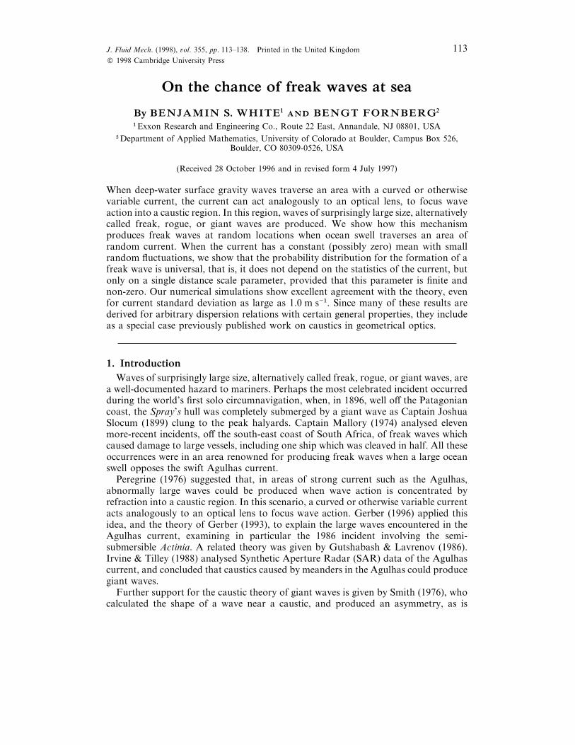
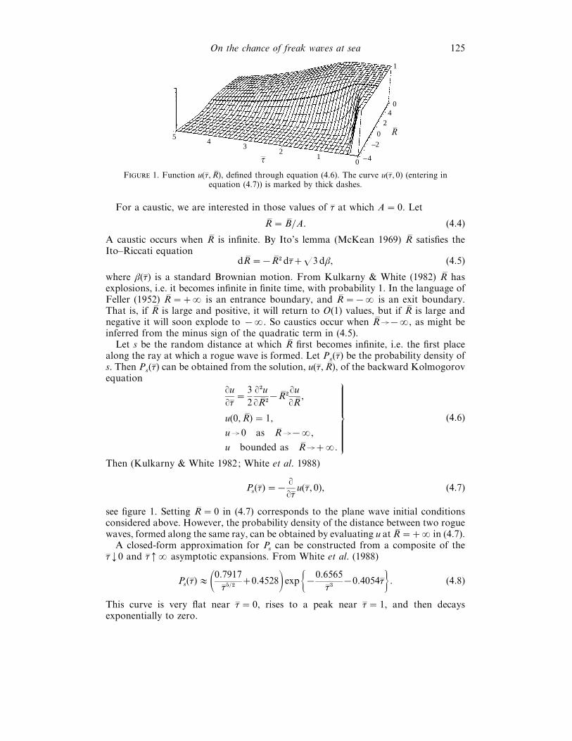
F 1. Function u(τa ,R ), defined through equation (4.6). The curve u(τa , 0) (entering inequation (4.7)) is marked by thick dashes.

For a caustic, we are interested in those values of τa at which A¯ 0. Let

R ¯B A. (4.4)

A caustic occurs when R is infinite. By Ito’s lemma (McKean 1969) R satisfies theIto–Riccati equation

dR ¯®R #dτa o3dβ, (4.5)

where β(τa ) is a standard Brownian motion. From Kulkarny & White (1982) R hasexplosions, i.e. it becomes infinite in finite time, with probability 1. In the language ofFeller (1952) R ¯¢ is an entrance boundary, and R ¯®¢ is an exit boundary.That is, if R is large and positive, it will return to O(1) values, but if R is large andnegative it will soon explode to ®¢. So caustics occur when R U®¢, as might beinferred from the minus sign of the quadratic term in (4.5).

Let s be the random distance at which R first becomes infinite, i.e. the first placealong the ray at which a rogue wave is formed. Let P

s(τa ) be the probability density of

s. Then Ps(τa ) can be obtained from the solution, u(τa ,R ), of the backward Kolmogorov

equation

¥u¥τa

¯3

2

¥#u¥R #

®R #¥u¥R ,

u(0,R )¯ 1,

uU 0 as R U®¢,

u bounded as R U¢.

5

6

7

8

(4.6)

Then (Kulkarny & White 1982; White et al. 1988)

Ps(τa )¯®

¥¥τa

u(τa , 0), (4.7)

see figure 1. Setting R ¯ 0 in (4.7) corresponds to the plane wave initial conditionsconsidered above. However, the probability density of the distance between two roguewaves, formed along the same ray, can be obtained by evaluating u at R ¯¢ in (4.7).

A closed-form approximation for Ps

can be constructed from a composite of theτa $ 0 and τa #¢ asymptotic expansions. From White et al. (1988)

Ps(τa )E 00.7917

τa &/#0.45281 exp (®0.6565

τa $®0.4054τa * . (4.8)

This curve is very flat near τa ¯ 0, rises to a peak near τa ¯ 1, and then decaysexponentially to zero.


LetD¯ c

gτa σ#/$ (4.9)

be the distance, to leading order, traversed along a ray at time τa . Then from (4.1), (4.3)

τa ¯ 0σ#aa %%g

12kW $ 93 cos#ψ®1

2 :#1"/$ D

cg

. (4.10)

As a specific model for a random current, let U be two-dimensionally incompressible,so that Uq is determined by a random stream function Ψ(x). Let Ψ have mean zero andcorrelation function

ρΨ(x«)¯©Ψ(x)Ψ(xx«)ª¯L#

4exp (®rx«r#

L#* . (4.11)

Here L is an intrinsic distance scale, and the pre-exponential factor is chosen so that©rUq r#ª¯ 1. For this model,

ρUq (x«)¯ exp (®rx«r#L#

*A

B

1

2®

x!#

#

L#

x!

"x!

#

L#

x!

"x!

#

L#

1

2®

x!#

"

L#

C

D

, (4.12)

and equation (4.10) becomes

τa ¯ (100π)"/'0σcg

1#/$ 0c!gcg

1#/$ 0cosψ 93 cos#ψ®1

2 :1#/$D

L, (4.13)

where c!g¯ "

#c!p

is the group velocity in the absence of current.When the mean current is zero, the third and fourth factors in (4.13) are unity. For

a non-trivial mean current, the situation may be more or less dangerous depending onthe average set and drift, with ψ¯ 54.7° the least dangerous situation, as discussed atthe beginning of this section. The most dangerous situation obtains when the swell isin a direction opposite to the set of the mean current, both according to (4.13) and inaccord with common lore. For a fixed mean current strength this situation bothmaximizes the terms involving cosψ and minimizes c

g, and gives a larger value of τa than

if the mean drift were zero. Note that this result is non-trivial, since a constant currentwith no random fluctuations will not by itself produce caustics in an opposing swell.

5. Numerical simulations

5.1. Description of the numerical ray tracing code

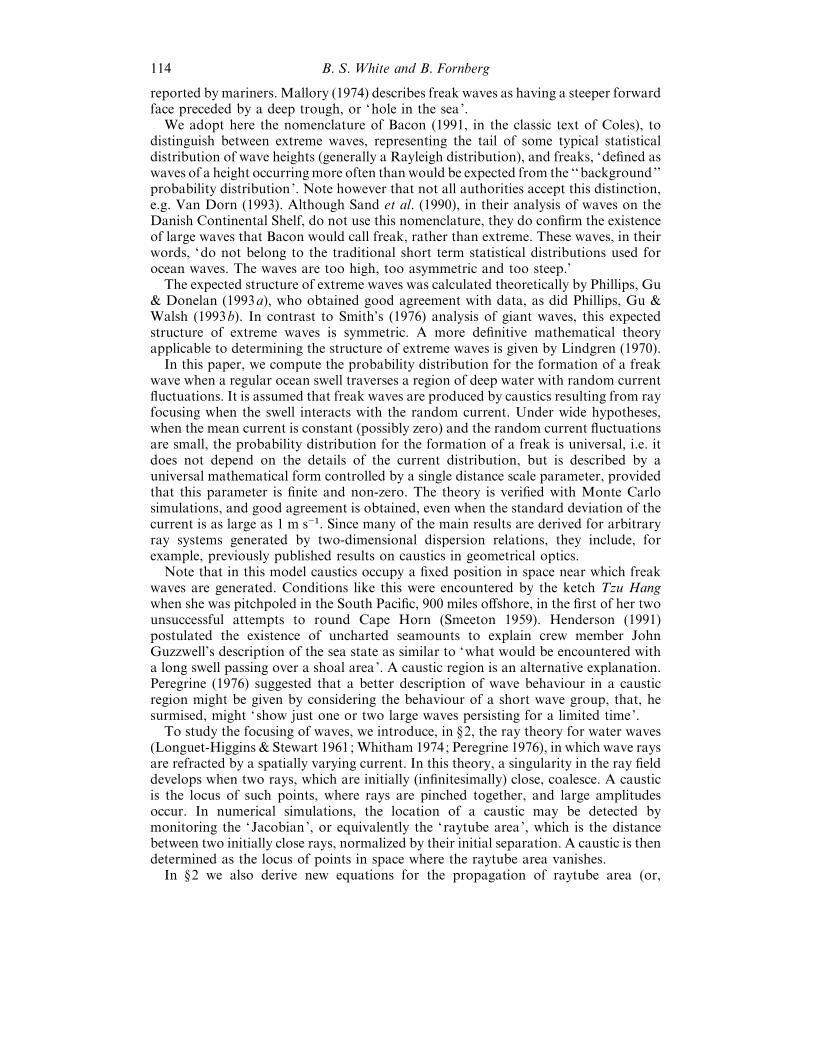
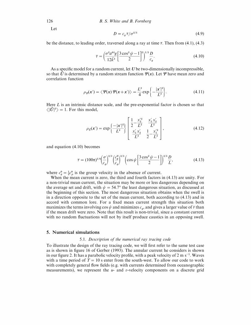
To illustrate the design of the ray tracing code, we will first refer to the same test caseas is shown in figure 16 of Gerber (1993). The annular current he considers is shownin our figure 2. It has a parabolic velocity profile, with a peak velocity of 2 m s−". Waveswith a time period of T¯ 10 s enter from the south-west. To allow our code to workwith completely general flow fields (e.g. with currents determined from oceanographicmeasurements), we represent the u- and -velocity components on a discrete grid


160 km

40 km

F 2. Ray tracing test problem: annular current ; parabolic velocity profile withmaximum velocity 2 m s−".

100

0

–100–200

–1000

100200

–200

–100

0

100

200

100

0

–100

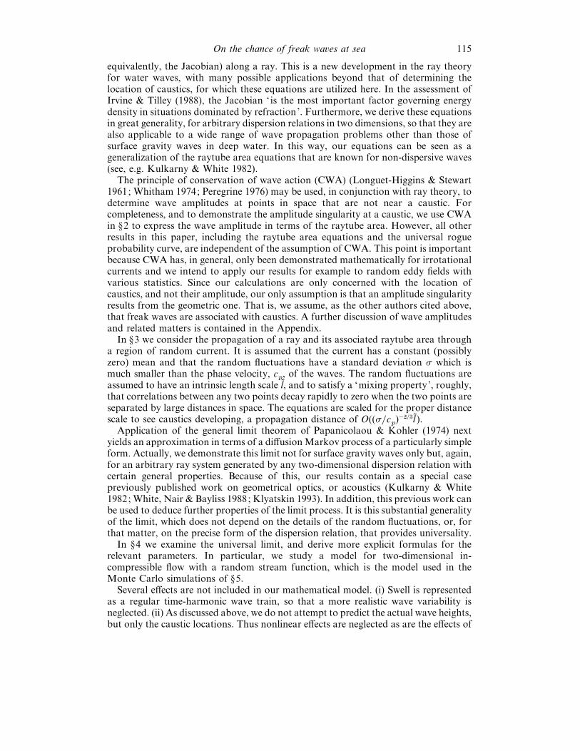
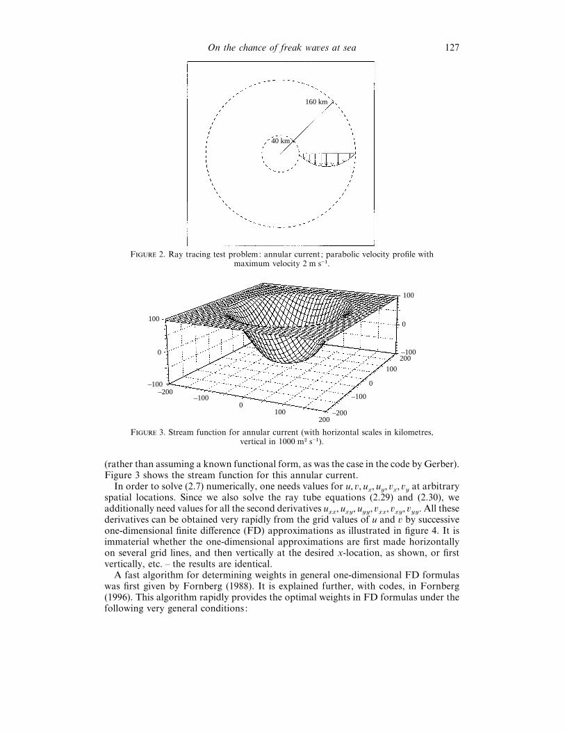
F 3. Stream function for annular current (with horizontal scales in kilometres,vertical in 1000 m# s−").

(rather than assuming a known functional form, as was the case in the code by Gerber).Figure 3 shows the stream function for this annular current.

In order to solve (2.7) numerically, one needs values for u, , ux, u

y,

x,

yat arbitrary

spatial locations. Since we also solve the ray tube equations (2.29) and (2.30), weadditionally need values for all the second derivatives u

xx, u

xy, u

yy,

xx,

xy,

yy. All these

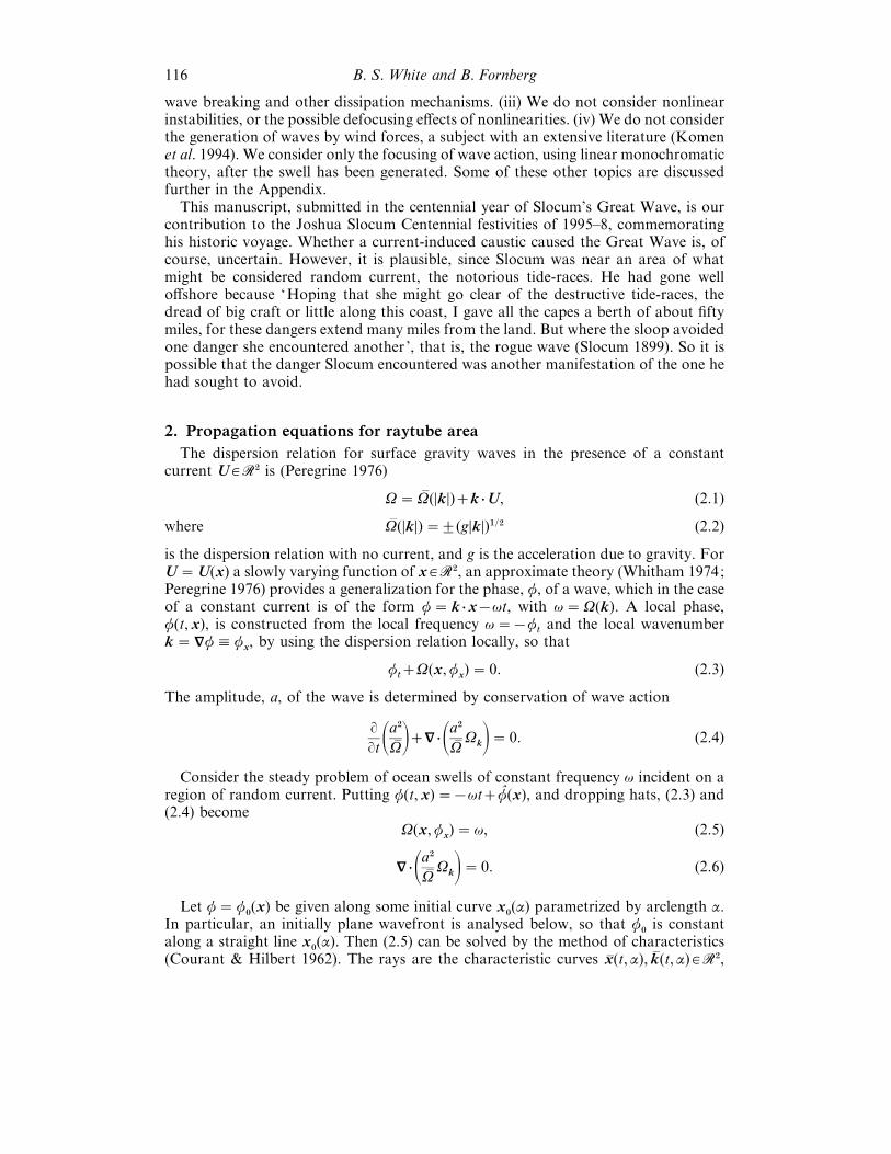
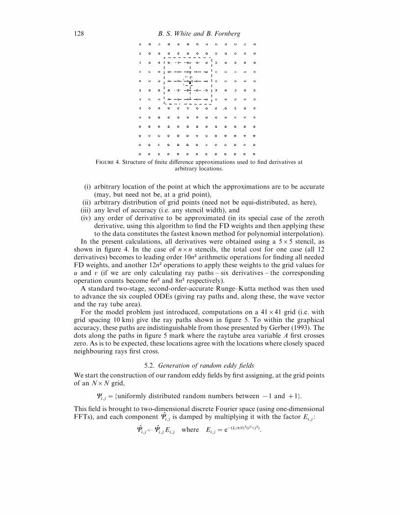
derivatives can be obtained very rapidly from the grid values of u and by successiveone-dimensional finite difference (FD) approximations as illustrated in figure 4. It isimmaterial whether the one-dimensional approximations are first made horizontallyon several grid lines, and then vertically at the desired x-location, as shown, or firstvertically, etc. – the results are identical.

A fast algorithm for determining weights in general one-dimensional FD formulaswas first given by Fornberg (1988). It is explained further, with codes, in Fornberg(1996). This algorithm rapidly provides the optimal weights in FD formulas under thefollowing very general conditions:


F 4. Structure of finite difference approximations used to find derivatives atarbitrary locations.

(i) arbitrary location of the point at which the approximations are to be accurate(may, but need not be, at a grid point),

(ii) arbitrary distribution of grid points (need not be equi-distributed, as here),(iii) any level of accuracy (i.e. any stencil width), and(iv) any order of derivative to be approximated (in its special case of the zeroth

derivative, using this algorithm to find the FD weights and then applying theseto the data constitutes the fastest known method for polynomial interpolation).

In the present calculations, all derivatives were obtained using a 5¬5 stencil, asshown in figure 4. In the case of n¬n stencils, the total cost for one case (all 12derivatives) becomes to leading order 10n# arithmetic operations for finding all neededFD weights, and another 12n# operations to apply these weights to the grid values foru and (if we are only calculating ray paths – six derivatives – the correspondingoperation counts become 6n# and 8n# respectively).

A standard two-stage, second-order-accurate Runge–Kutta method was then usedto advance the six coupled ODEs (giving ray paths and, along these, the wave vectorand the ray tube area).

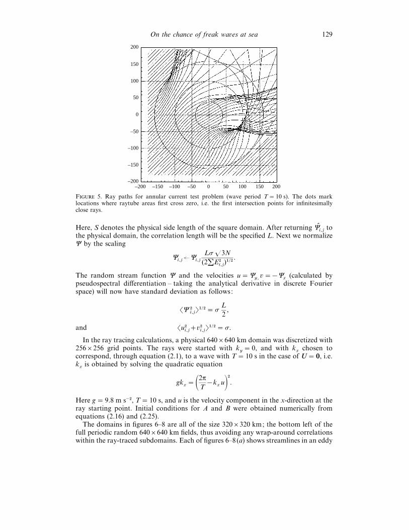
For the model problem just introduced, computations on a 41¬41 grid (i.e. withgrid spacing 10 km) give the ray paths shown in figure 5. To within the graphicalaccuracy, these paths are indistinguishable from those presented by Gerber (1993). Thedots along the paths in figure 5 mark where the raytube area variable A first crosseszero. As is to be expected, these locations agree with the locations where closely spacedneighbouring rays first cross.

5.2. Generation of random eddy fields

We start the construction of our random eddy fields by first assigning, at the grid pointsof an N¬N grid,

Ψi,j

¯²uniformly distributed random numbers between ®1 and 1´.

This field is brought to two-dimensional discrete Fourier space (using one-dimensionalFFTs), and each component Ψq

i,jis damped by multiplying it with the factor E

i,j:

Ψqi,j

VΨqi,j

Ei,j

where Ei,j

¯ e−(L/πS)#(i

#+j

#).


200

150

100

50

–50

–100

–150

–200

0

–200 –150 –100 –50 0 50 100 150 200

F 5. Ray paths for annular current test problem (wave period T¯ 10 s). The dots marklocations where raytube areas first cross zero, i.e. the first intersection points for infinitesimallyclose rays.

Here, S denotes the physical side length of the square domain. After returning Ψqi,j

tothe physical domain, the correlation length will be the specified L. Next we normalizeΨ by the scaling

Ψi,j

VΨi,j

Lσo3N

(23E#i,j

)"/#.

The random stream function Ψ and the velocities u¯Ψy,

¯®Ψx

(calculated bypseudospectral differentiation – taking the analytical derivative in discrete Fourierspace) will now have standard deviation as follows:

©Ψ #i,j

ª"/#¯σL

2,

and ©u#i,j

#i,j

ª"/#¯σ.

In the ray tracing calculations, a physical 640¬640 km domain was discretized with256¬256 grid points. The rays were started with k

y¯ 0, and with k

xchosen to

correspond, through equation (2.1), to a wave with T¯ 10 s in the case of U¯0, i.e.kx

is obtained by solving the quadratic equation

gkx¯ 02π

T®k

xu1#.

Here g¯ 9.8 m s−#, T¯ 10 s, and u is the velocity component in the x-direction at theray starting point. Initial conditions for A and B were obtained numerically fromequations (2.16) and (2.25).

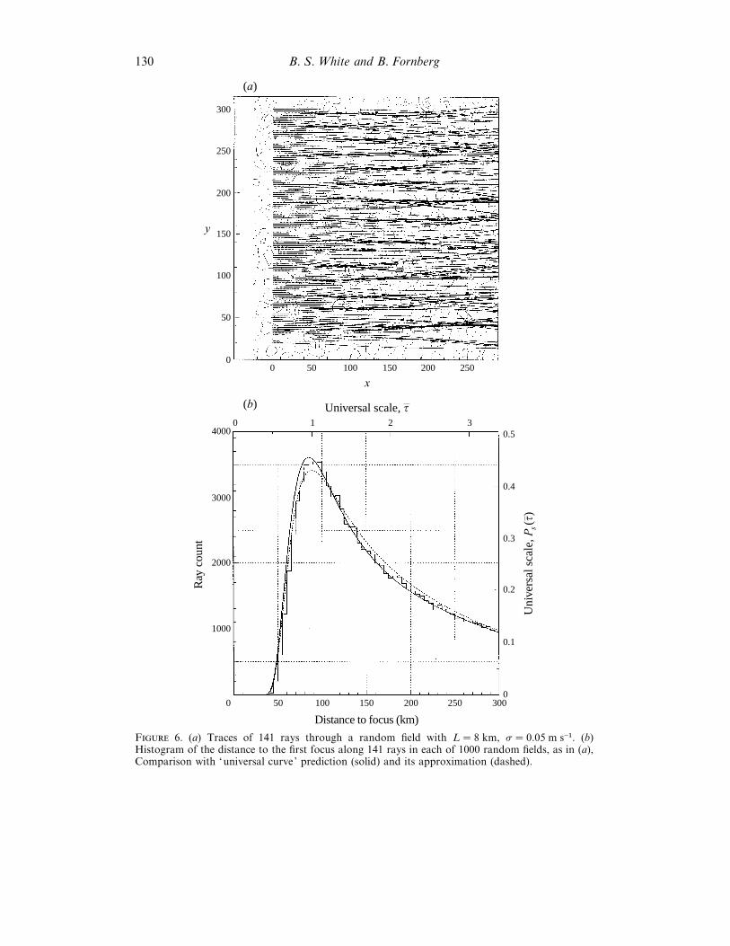
The domains in figures 6–8 are all of the size 320¬320 km; the bottom left of thefull periodic random 640¬640 km fields, thus avoiding any wrap-around correlationswithin the ray-traced subdomains. Each of figures 6–8(a) shows streamlines in an eddy


300

250

200

150

100

50

00 50 100 150 200 250

x

y

(a)

4000

3000

2000

1000

0 50 100 150 200 250 3000

0.1

0.2

0.3

0.4

0.53210

Ray

cou

nt

Distance to focus (km)

Universal scale, s

Uni

vers

al s

cale

, Ps(s

)

(b)

F 6. (a) Traces of 141 rays through a random field with L¯ 8 km, σ¯ 0.05 m s−". (b)Histogram of the distance to the first focus along 141 rays in each of 1000 random fields, as in (a),Comparison with ‘universal curve’ prediction (solid) and its approximation (dashed).


300

250

200

150

100

50

00 50 100 150 200 250

x

y

(a)

4000

3000

2000

1000

0 50 100 150 200 250 3000

0.1

0.2

0.3

0.4

0.53210

Ray

cou

nt


Universal scale, s

Uni

vers

al s

cale

, Ps(s

)

(b)

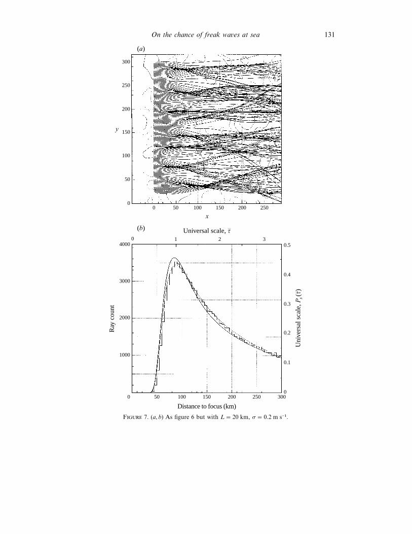
F 7. (a, b) As figure 6 but with L¯ 20 km, σ¯ 0.2 m s−".


300

250

200

150

100

50

00 50 100 150 200 250

x

y

(a)

4000

3000

2000

1000

0 50 100 150 200 250 3000

0.1

0.2

0.3

0.4

0.5

3210

Ray

cou

nt


Universal scale, s

Uni

vers

al s

cale

, Ps(s

)

(b)

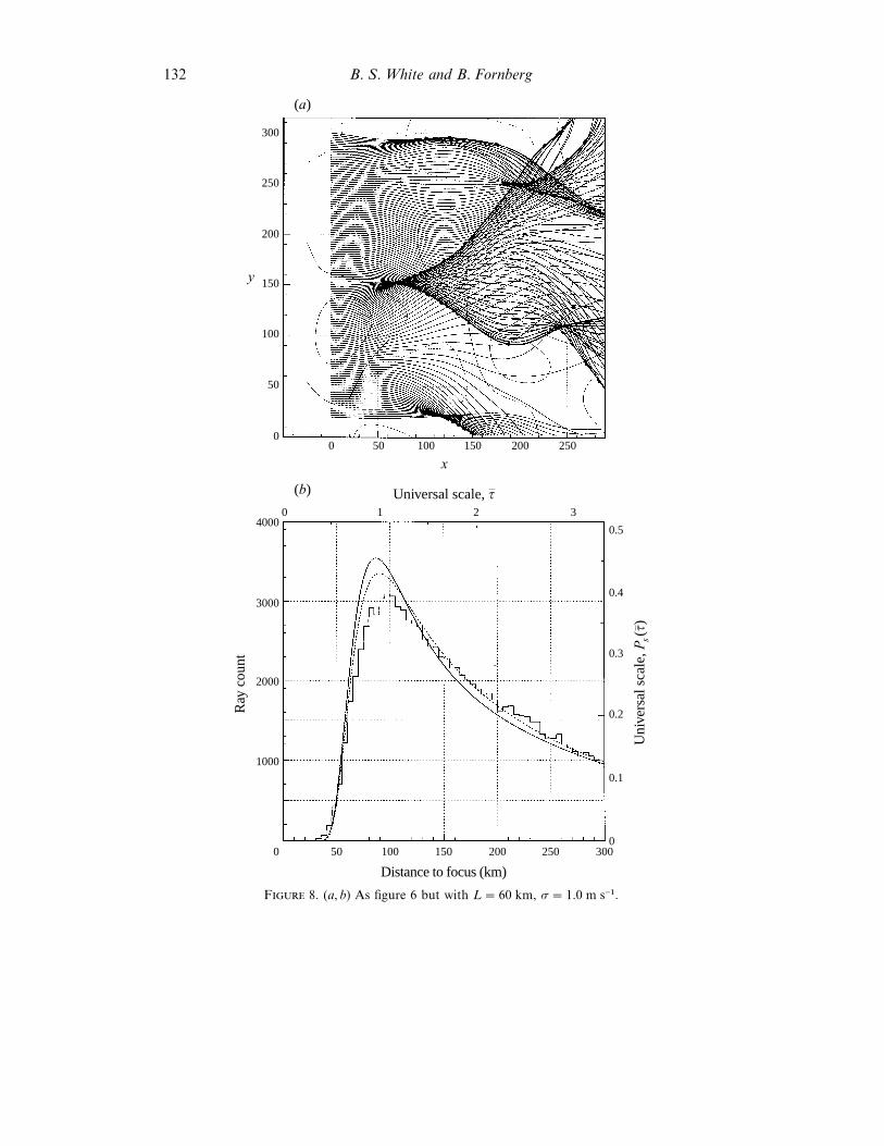
F 8. (a, b) As figure 6 but with L¯ 60 km, σ¯ 1.0 m s−".


800

0

–800

250

200

150

100

50

0 050

100

200150

250y

x

(a)

8000

0

–8000

250

200

150

100

50

0 050

100

200150

250y

x

(b)

80000

0

–80000

250

200

150

100

50

0 050

100

200150

250y

x

(c)

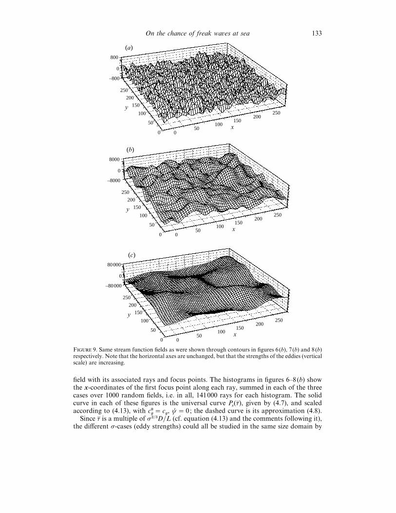
F 9. Same stream function fields as were shown through contours in figures 6(b), 7(b) and 8(b)respectively. Note that the horizontal axes are unchanged, but that the strengths of the eddies (verticalscale) are increasing.

field with its associated rays and focus points. The histograms in figures 6–8(b) showthe x-coordinates of the first focus point along each ray, summed in each of the threecases over 1000 random fields, i.e. in all, 141000 rays for each histogram. The solidcurve in each of these figures is the universal curve P

s(τa ), given by (4.7), and scaled

according to (4.13), with c!g¯ c

g, ψ¯ 0; the dashed curve is its approximation (4.8).

Since τa is a multiple of σ#/$DL (cf. equation (4.13) and the comments following it),the different σ-cases (eddy strengths) could all be studied in the same size domain by


suitably adjusting L. Figure 9(a–c) illustrates again these scalings; the three surfacesshow the same three stream function fields as were previously seen in figures 6–8(a).Note the differences in the vertical scale in the three cases.

6. Conclusions

We have demonstrated that a single universal curve, when appropriately scaled, willaccurately describe the distribution of focus points, that is, areas of particularly intensewave action, which will arise when uniform waves enter a region of random current.Although in the theoretical derivation of this curve it was assumed that the randomcurrent fluctuations were small, and therefore that focusing would occur only after thewaves have travelled through many random eddies, the numerical calculations showedexcellent agreement with theory even when random effects were relatively large – withfocusing occurring before even a single eddy has been traversed. Since σ¯ 1 m s−", i.e.a velocity standard deviation of about 2 knots, represents a substantial current, weexpect that these results will be generally applicable. If an estimate can be made of thedistance scale parameter, and of the distance propagated through the random currentfield, reference to the universal curve provides a quantitative estimate of the danger ofa rogue wave.

Appendix

In this manuscript we are directly concerned only with the chance of a freak waveat sea, and not with the chance factors influencing the height, steepness, asymmetricshape or any other properties of the giant wave itself. That is, we are concerned withthe likelihood of encountering a freak wave, rather than an estimation of the expecteddamage from encountering one. We also neglect nonlinear effects which may causeinstability or defocusing of the waves. Since a study of these related issues would makea useful complement to the present work, we will briefly review them here.

As discussed in the Introduction, even for points in space that are not near caustics,principles such as conservation of wave action (CWA), that would enable calculationof amplitudes, lack a firm mathematical basis when the current has non-zero vorticity.For water of finite depth, with wave modulations that are long compared to the depth,CWA can be justified, even with rotational currents, by the work of Stiassnie &Peregrine (1979). However, it might be argued that waves on a deep current do notsatisfy CWA, based on the form of the nonlinear Schro$ dinger equation (NLS) derivedfor the amplitude by Mei (1989, equation (2.59) on p. 618) (NLS methods are discussedfurther below). Still, the application of CWA to rotational currents remainscontroversial.

Many authors have not been inhibited by its deficiencies from using ray theory tocompute amplitudes in the presence of rotational currents, e.g. the example of Gerber(1993) which we considered in §5. Also, Peregrine (1976, §IIE) used CWA for waveson a shear current for his investigation of freak waves and caustics. In particular, aform of CWA is often used in computing wave spectra, regardless of vorticity. Forexample, Mathiesen (1987) computed wave refraction by a current whirl, and Mapp,Welch & Munday (1985) got good agreement of their ray theoretic energy densitieswith those determined by Synthetic Aperture Radar (SAR) data, for observations ofwaves refracted by warm core rings. Irvine & Tilley (1988) used CWA to interpret theirSAR data of the Agulhas current. Their analysis of meanders supports the basichypothesis of our manuscript : the theory that giant waves are caused by current-


induced caustics. In their assessment, CWA ‘represents the presently accepted core ofbelief ’.

Near a caustic, even CWA is not sufficient for the determination of amplitudes.Other factors include: finite frequency diffraction effects that mitigate the causticsingularity ; nonlinearities that can cause defocusing and instabilities ; blurring of thecaustic because real ocean waves are a mixture of frequencies rather than the puremonochromatic waves used in the mathematical model ; wave energy generation bywind forces ; and energy dissipation from breaking waves. An overview of some ofthese factors is given in the review lecture of Peregrine (1985).

Linear theory predicts that the amplitude singularity near a caustic of simple raytheory will be mitigated by finite frequency diffraction effects. The maximumamplitude, and the size of the caustic boundary layer within which diffractioncorrections are needed, are both determined as powers of spatial frequency k, with theexact powers dependent on the geometry of the caustic. Of course, in the present work,the size of the caustic boundary layer, as well as the wavelength, is assumed to be muchsmaller than the correlation length of the random medium. For non-dispersive wavesa uniform expansion for a smooth caustic was given by Ludwig (1966), and anexpansion near the cusp of a caustic was given by Pearcey (1946).

Alternatively, the Gaussian beam summation method can capture caustic correctionsfor caustics of arbitrary geometric complexity (White et al. 1987). An adaptation of thismethod, combined with stochastic methods that parallel those of the present paper, hasbeen used to compute wave statistics for wave propagation problems where causticsoccur at random locations (Nair & White 1991).

Another approach to calculating diffraction at a caustic is the parabolic equationapproximation for the amplitude, and a variant of this approach, the nonlinearSchro$ dinger equation (NLS), can be adapted to include weak nonlinear effects. Smith(1976) used this method in his analysis of giant waves, and estimated that for freakwaves in the Agulhas current, there would be ‘about a three-fold amplification of thewave height near the caustic ’. He also noted that even a doubling of height would be‘quite traumatic ’.

Peregrine (1986) gave two simple approximations for wave amplitude at the cusp ofa caustic, for water waves propagating over underwater shoals and spurs. One of hisapproximations is based on the linear theory of Pearcey (1946), and the other, whichincludes weak nonlinear effects, is based on the NLS. The NLS method for thisproblem was compared with tank tests by Peregrine et al. (1988), and they obtainedgood quantitative agreement. While they observed the predicted defocusing effects ofnonlinearity, they noted that linear diffraction is also important, and can be dominantin practical cases.

A nonlinear mechanism quite different from that of caustic formation has beenproposed as an alternative explanation of freak waves. Dean (1990) suggested that thenonlinear superposition of waves might produce waves larger than those suggested bylinear superposition. The resulting statistical distribution of wave heights would thenhave large waves occurring more frequently than predicted by the Rayleighdistribution. These large waves would then be, by definition, freaks.

Nonlinearities can also cause instability of a regular wave train. This was firstdemonstrated theoretically by Benjamin & Feir (1967), who showed that for weaklynonlinear surface gravity waves in deep water, regular wave trains were unstable toperturbations, a result confirmed in the experimental work of Feir (1967) and others(see Su et al. 1982 and references therein). Some of this experimental work showed thatthe initial instability does not necessarily lead to disintegration of the wave train.


Instead, as in Su et al. (1982), the waves can evolve first into a series of crescent-shaped,spilling breakers, and then, finally, to a series of wave groups with a peak frequencythat is lower than the frequency of the initial wave train.

Gerber (1987) investigated a variation of the Benjamin–Feir instability, relevant towave packets propagating in deep water with non-uniform currents. He found anenhancement of the instability for waves travelling against an adverse current, whilethe current had a stabilizing effect for waves travelling with it. Most relevant for thepresent work, he found enhanced instability of the wave packet in the neighbourhoodof a caustic caused by a shear current.

The Benjamin–Feir instability is one reason why a perfectly regular time-harmonicwave train is an idealized model. In practice, even a relatively regular ocean swellcontains a mixture of frequencies. Since surface gravity waves are dispersive, eachfrequency will give a caustic in a different location, as will, for instance, variations inthe initial direction of the waves. Even if all these variations are small, the sharplydefined caustic for monochromatic unidirectional waves will be blurred, and this mayhave a significant effect on amplitudes. However, even though both nonlinearity anda broad spectrum of frequencies are thought to have defocusing effects, thecombination of nonlinearity and broad spectrum has been proposed as the cause offreak waves by Trulsen & Dysthe (1996). Consequently, these authors have derived aform of the NLS equation applicable to a broad spectrum of frequencies, but have notyet demonstrated that this equation will generate freak waves.

To return to the question of amplitude, we note that amplitude, or wave height, isnot necessarily the best measure of danger for a vessel at sea. Wave steepness is alsoimportant, since even a small vessel can ride over large, but long seas provided they arenot too steep, a situation that often prevails in the Southern Ocean. Wave breaking isanother important feature. In their review of model tests, actual capsizes, andmathematical, statistical and engineering analyses, Kirkman & McCurdy (1987)concluded that ‘As a rule, we believe, no non-breaking wave is dangerous’ for offshoreyachts. Kjeldsen (1990) has derived a theory for calculating wave loads and slammingcaused by freak waves which are breaking, and presented some comparisons withoceanographic measurements. Kjeldsen’s work is in response to what he perceived asthe cause of capsize for the 26 Norwegian ships lost in the period 1970–78, 13 of themwith no survivors.

Some of the factors that cause wave breaking were investigated in the numericalcomputations of Dold & Peregrine (1986). These authors observed the growth of smallmodulations on regular wave trains, as predicted by the Benjamin–Feir instability, anddetermined the ranges of wave steepness and modulation length necessary for deepwater waves to break.

Details of the wave shape can also be important in assessing danger. For examplethe deep trough, or ‘hole in the sea’, often reported preceding a freak wave, presentsa special hazard, as explained by Mallory (1974). When a fast ship meets a freak wavehead-on, she first steams downward into the trough, burying her bow. Now theforward part of a ship usually has great buoyancy. So the bow forcefully attempts torise just as the giant wave breaks on deck aft of the ship’s forward buoyant area. Theresulting shear forces on the hull can cause significant structural damage, usually nearthe bulkhead between Nos. 1 and 2 hatches.


REFERENCES

B, S. 1991 Wind waves. In Heay Weather Sailing (ed. K. Adlard Coles), 4th edn. InternationalMarine.

B, T. B. & F, J. E. 1967 The disintegration of wave trains on deep water. Part 1. Theory.J. Fluid Mech. 27, 417–430.

C, R. & H, D. 1962 Methods of Mathematical Physics, Vol. II. Interscience.

D, R. G. 1990 Freak waves : A possible explanation. In Water Wae Kinematics (ed. A. Torum& O. T. Gudmestad), pp. 609–612. Kluwer.

D, J. W. & P, D. H. 1986 Water-wave modulation. In Proc. 20th Intl Conf. on CoastalEngng vol. 1, Chap 13, pp. 163–175.

F, J. E. 1967 Discussion: some results from wave pulse experiments. Proc. R. Soc. Lond. A 299,54–58.

F, W. 1952 The parabolic differential equations and associated semi-groups of trans-formations. Ann. Maths 55, 468–519.

F, B. 1988 Generation of finite difference formulas on arbitrarily spaced grids. Math.Comput. 51, 699–706.

F, B. 1996 A Practical Guide to Pseudospectral Methods. Cambridge University Press.

G, M. 1987 The Benjamin–Feir instability of a deep-water stokes wavepacket in the presenceof a non-uniform medium. J. Fluid Mech. 176, 311–332.

G, M. 1993 The interaction of deep-water gravity waves and an annular current : linear theory.J. Fluid Mech. 248, 153–172.

G, M. 1996 Giant waves and the Agulhas Current. Deep-Sea Res. (submitted).

G, Y. S & L, I. V. 1986 Swell transformation in the Cape Agulhas current.Iz. Atmos. Ocean. Phys. 22, No. 6, 494–497.

H, R. 1991 Sea Sense, p. 299. International Marine.

H, L. & S, B. 1988 Propagation of weak shocks through a random medium.J. Fluid Mech. 196, 513–553.

I, D. E. & T, D. G. 1988 Ocean wave directional spectra and wave-current interaction inthe Agulhas from the shuttle imaging radar-B synthetic aperture radar. J. Geophys. Res. 93,15,389–15,401.

K, K. L. & MC, R. C. 1987 Avoiding capsize : research work. In Desirable andUndesirable Characteristics of Offshore Yachts (ed. J. Rousmaniere), pp. 57–74. TechnicalCommittee of the Cruising Club of America, Nautical Quarterly Books, W. W. Norton.

K, S. P. 1990 Breaking waves. In Water Wae Kinematics (ed. A. Torum & O. T.Gudmestad), pp. 453–473. Kluwer.

K, V. I. 1993 Caustics in random media. Waes in Random Media 3, 93–100.

K, G. J. et al. (Eds.) 1994 Dynamics and Modelling of Ocean Waes. (subtitle : Final report ofthe WAM group) Cambridge University Press.

K, V. A. & W, B. S. 1982 Focusing of waves in turbulent inhomogeneous media. Phys.Fluids 25, 1770–1784.

L, G. 1970 Some properties of a normal process near a local maximum. Ann. Math. Statist.41, 1870–1883.

L-H, M. S. & S, R. W. 1961 The changes in amplitude of short gravity waveson steady non-uniform currents. J. Fluid Mech. 10, 529–549.

L, D. 1966 Uniform asymptotic expansions at a caustic. Commun. Pure Appl. Maths 19,215–250.

M, J. K. 1974 Abnormal waves on the south east coast of South Africa. Intl Hydrog. Re.51, 99–129.

M, G. R., W, C. S. & M, J. C. 1985 Wave refraction by warm core rings. J. Geophys.Res. 90, 7153–7162.

M, M. 1987 Wave refraction by a current whirl. J. Geophys. Res. 92, 3905.

MK, H. P. 1969 Stochastic Integrals. Academic.

M, C. C. 1989 The Applied Dynamics of Ocean Surface Waes. World Scientific.


N, B. & W, B. S. 1991 High-frequency wave propagation in random media – a unifiedapproach. SIAM J. Appl. Maths 51, 374–411.

P, G. & K, W. 1974 Asymptotic theory of mixing stochastic ordinary differentialequations. Commun. Pure Appl. Maths 27, 641–668.

P, T. 1946 The structure of an electromagnetic field in the neighborhood of a cusp of acaustic. Lond. Edinb. Dublin Phil. Mag. (7) 37, 311–317.

P, D. H. 1976 Interaction of water waves and currents. Ad. Appl. Mech. 16, 9–117.

P, D. H. 1985 Water waves and their development in space and time. Proc. R. Soc. Lond.A 400, 1–18.

P, D. H. 1986 Approximate descriptions of the focussing of water waves. Proc. 20th IntlConf. Coastal Engng, vol. 1, Chap. 51, pp. 675–685.

P, D. H., S, D., S, M. & D, N. 1988 Nonlinear effects on focussed waterwaves. Proc. 21st Intl Conf. Coastal Engng, vol. 1, Chap. 54, pp. 732–742.

P, O. M., G, D. & D, M. 1993a Expected structure of extreme waves in a Gaussiansea. Part I : Theory and swade buoy measurements. J. Phys. Oceanogr. 23, 992–1000.

P, O. M., G, D. & W, E. 1993b On the expected structure of extreme waves in aGaussian sea. Part II : SWADE Scanning Radar Altimeter Measurements. J. Phys. Oceanogr.23, 2297–2309.

S, S. E. et al. 1990 Freak wave kinematics. In Water Wae Kinematics (ed. A. Torum &O. T. Gudmestad), pp. 535–549. Kluwer.

S, J. 1899 Sailing Alone Around the World, Chap. VIII. The Century Co. (Reprinted 1954Sheridan House.)

S, M. 1959 Once is Enough. Rupert Hart-Davis Ltd. (Reprinted 1991, Billings and Sons Ltd.)

S, R. 1976 Giant waves. J. Fluid Mech. 77, 417–431.

S, M. & P, D. H. 1979 On averaged equations for finite amplitude water waves.J. Fluid Mech. 94, 401–407.

S, M.-Y., B, M., M, P. & M, R. 1982 Experiments on nonlinear instabilities andevolution of steep gravity-wave trains. J. Fluid Mech. 124, 45–72.

T, K. & D, K. B. 1996 Freak waves : a 3-D wave simulation. In Proc. 21st Intl Symp.on Naal Hydrodynamics. Trondheim, Norway.

V D, W. G. 1993 Oceanography and Seamanship. 2nd Edn. Cornell Maritime Press.

W, B. S. 1984 The stochastic caustic. SIAM J. Appl. Maths 44, 127–149.

W, B., N, B. & B, A. 1988 Random rays and seismic amplitude anomalies. Geophysics53, 903–907.

W, B. S., N, A., B, A. & B, R. 1987 Some remarks on the Gaussian beamsummation method. Geophys. J. R. Astron. Soc. 89, 579–636.

W, G. B. 1974 Linear and Non-Linear Waes. Wiley-Interscience.

Z, D. I. & W, B. S. 1985 Propagation of initially plane waves in the region of randomcaustics. Wae Motion 7, 202–227.

on the chance of freak waves at sea - citeseer

Documents