On the Classification of Holonomy Representations

Habilitationsschrift

zur Erlangung des akademischen Grades

Dr. rer. nat. habil.

der Fakultat fur Mathematik und Informatikder Universitat Leipzig

eingereicht von

Dr. Lorenz Johannes Schwachhofer

geboren am 7. Januar 1964 in Offenbach am Main

angefertigt am Mathematischen Institutder Universitat Leipzig

Beschluß uber die Verleihung des akademischen Grades vom22. Juni 1998

Die Annahme der Habilitationsschrift haben empfohlen:

1. Prof. Dr. Hans-Bert Rademacher, Universitat Leipzig

2. Prof. Dr. Robert Bryant, Duke University, Durham, USA

3. Prof. Dr. Wolfgang Ziller, University of Pennsylvania, Philadelphia, USA

Bibliographische Beschreibung:

Schwachhofer, Lorenz JohannesOn the Classification of Holonomy RepresentationsUniversitat Leipzig, Diss.,66 S., 49 Lit.

Referat:

Die Arbeit befaßt sich mit der Klassifikation irreduzibler Holonomiegruppen torsionsfreier Zusammen-hange und deren Anwendungen in der Differentialgeometrie und der komplexen Analysis.

Das Klassifikationsproblem geht auf E. Cartan zuruck, der in den zwanziger Jahren den Holonomiebegriffeinfuhrte. Von den funfziger Jahren an wurde zunachst die Untersuchung der moglichen Holonomiegrup-pen Riemannscher Mannigfaltigkeiten zu einem zentralen Problem in der Differentialgeometrie, das erst inden achziger Jahren vollstandig gelost werden konnte. Anfang der neunziger Jahre wuchs jedoch auch dasInteresse an nicht-Riemannschen Zusammenhangen, vor allem weil solche Zusammenhange auf gewissen Mod-ulraumen von Legendremannigfaltigkeiten in naturlicher Weise auftreten und sich somit auch Konsequenzenfur die komplexe Deformationstheorie ergeben. In den letzten funf Jahren wurden zunachst mehrere neueHolonomiegruppen entdeckt. Vor einem Jahr erfolgte schließlich in gemeinsamer Arbeit mit S. Merkulovdie vollstandige Klassifikation aller Holonomiegruppen und somit die Losung des Holonomieproblems imirreduziblen Falle.

Den zentralen Teil dieser Habilitationsschrift bildet das dritte Kapitel. Dort erfolgt zunachst eine genauereUntersuchung der Relation von reellen und komplexen Bergeralgebren. Dadurch wird es moglich, die Klas-sifikation in der komplexen Kategorie durchzufuhren. Danach erfolgt eine Reihe von Beispielen neuer Berg-eralgebren. Die Moglichkeit der zentralen Erweiterung von Holonomiedarstellungen und die Existenz sym-metrischer Zusammenhange wird eingehend untersucht. Schließlich wird ein neuer, vereinfachter Beweis derKlassifikation von Bergeralgebren gegeben. Die Vereinfachung besteht darin, daß der hier vorgestellte Be-weis lediglich die Methoden der klassischen Darstellungstheorie verwendet, wahrend der ursprungliche Beweisneben klassischer Darstellungstheorie auch Mittel aus der komplexen Analysis benutzte. Letzteres erschienjedoch fur die Losung dieses im wesentlichen darstellungstheoretischen Problems sehr unbefriedigend; zudemist der hier vorgestellte Beweis kurzer.

Im vierten Kapitel werden dann noch die wichtigsten Methoden beschrieben, die zeigen, daß jede Berg-eralgebra auch tatsachlich als Holonomiegruppe auftritt. Zum einen ist dies der Ansatz von R. Bryant,der das Existenzproblem mittels eines “Exterior Differential System” beschreibt, und zum anderen eine ingemeinsamer Arbeit mit Q.-S. Chi und S. Merkulov entwickelte Methode, die auf einer gewissen Deformationder Poissonstruktur einer dualen Liealgebra beruht.

Schließlich wird im letzten Kapitel noch eine twistortheoretische Beschreibung holomorpher torsionsfreierZusammenhange gegeben, die im wesentlichen auf S. Merkulov zuruckgeht.

2

Contents

1 Introduction and history 4

2 Preliminary facts and results 82.1 Holonomy groups and holonomy algebras . . . . . . . . . . . . . . . . . . . . . . . . . . . . . 82.2 Spencer cohomology . . . . . . . . . . . . . . . . . . . . . . . . . . . . . . . . . . . . . . . . . 102.3 H-structures, intrinsic torsion and intrinsic curvature . . . . . . . . . . . . . . . . . . . . . . . 112.4 A brief review of representation theory . . . . . . . . . . . . . . . . . . . . . . . . . . . . . . . 13

3 Berger algebras 153.1 Real Berger algebras . . . . . . . . . . . . . . . . . . . . . . . . . . . . . . . . . . . . . . . . . 153.2 Examples of Berger algebras . . . . . . . . . . . . . . . . . . . . . . . . . . . . . . . . . . . . . 17

3.2.1 Conformal Lie algebras . . . . . . . . . . . . . . . . . . . . . . . . . . . . . . . . . . . 173.2.2 Symplectic Lie algebras . . . . . . . . . . . . . . . . . . . . . . . . . . . . . . . . . . . 183.2.3 Symmetric connections . . . . . . . . . . . . . . . . . . . . . . . . . . . . . . . . . . . . 203.2.4 Complex Lie algebras with h(1) 6= 0 . . . . . . . . . . . . . . . . . . . . . . . . . . . . . 21

3.3 Complex Berger algebras . . . . . . . . . . . . . . . . . . . . . . . . . . . . . . . . . . . . . . . 223.4 Simple complex Berger algebras . . . . . . . . . . . . . . . . . . . . . . . . . . . . . . . . . . . 233.5 Complex tensor representations . . . . . . . . . . . . . . . . . . . . . . . . . . . . . . . . . . . 34

4 Existence results 364.1 Exterior Differential Systems . . . . . . . . . . . . . . . . . . . . . . . . . . . . . . . . . . . . 374.2 Poisson manifolds . . . . . . . . . . . . . . . . . . . . . . . . . . . . . . . . . . . . . . . . . . . 384.3 Symplectic torsion free connections . . . . . . . . . . . . . . . . . . . . . . . . . . . . . . . . . 40

5 Twistor theory of torsion free connections 44

References 50

3

1 Introduction and history

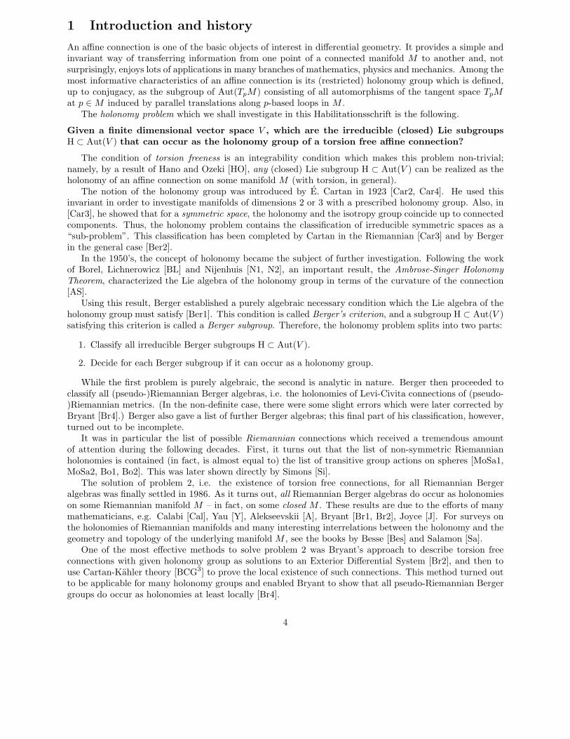
An affine connection is one of the basic objects of interest in differential geometry. It provides a simple andinvariant way of transferring information from one point of a connected manifold M to another and, notsurprisingly, enjoys lots of applications in many branches of mathematics, physics and mechanics. Among themost informative characteristics of an affine connection is its (restricted) holonomy group which is defined,up to conjugacy, as the subgroup of Aut(TpM) consisting of all automorphisms of the tangent space TpMat p ∈M induced by parallel translations along p-based loops in M .

The holonomy problem which we shall investigate in this Habilitationsschrift is the following.

Given a finite dimensional vector space V , which are the irreducible (closed) Lie subgroupsH ⊂ Aut(V ) that can occur as the holonomy group of a torsion free affine connection?

The condition of torsion freeness is an integrability condition which makes this problem non-trivial;namely, by a result of Hano and Ozeki [HO], any (closed) Lie subgroup H ⊂ Aut(V ) can be realized as theholonomy of an affine connection on some manifold M (with torsion, in general).

The notion of the holonomy group was introduced by E. Cartan in 1923 [Car2, Car4]. He used thisinvariant in order to investigate manifolds of dimensions 2 or 3 with a prescribed holonomy group. Also, in[Car3], he showed that for a symmetric space, the holonomy and the isotropy group coincide up to connectedcomponents. Thus, the holonomy problem contains the classification of irreducible symmetric spaces as a“sub-problem”. This classification has been completed by Cartan in the Riemannian [Car3] and by Bergerin the general case [Ber2].

In the 1950’s, the concept of holonomy became the subject of further investigation. Following the workof Borel, Lichnerowicz [BL] and Nijenhuis [N1, N2], an important result, the Ambrose-Singer HolonomyTheorem, characterized the Lie algebra of the holonomy group in terms of the curvature of the connection[AS].

Using this result, Berger established a purely algebraic necessary condition which the Lie algebra of theholonomy group must satisfy [Ber1]. This condition is called Berger’s criterion, and a subgroup H ⊂ Aut(V )satisfying this criterion is called a Berger subgroup. Therefore, the holonomy problem splits into two parts:

1. Classify all irreducible Berger subgroups H ⊂ Aut(V ).

2. Decide for each Berger subgroup if it can occur as a holonomy group.

While the first problem is purely algebraic, the second is analytic in nature. Berger then proceeded toclassify all (pseudo-)Riemannian Berger algebras, i.e. the holonomies of Levi-Civita connections of (pseudo-)Riemannian metrics. (In the non-definite case, there were some slight errors which were later corrected byBryant [Br4].) Berger also gave a list of further Berger algebras; this final part of his classification, however,turned out to be incomplete.

It was in particular the list of possible Riemannian connections which received a tremendous amountof attention during the following decades. First, it turns out that the list of non-symmetric Riemannianholonomies is contained (in fact, is almost equal to) the list of transitive group actions on spheres [MoSa1,MoSa2, Bo1, Bo2]. This was later shown directly by Simons [Si].

The solution of problem 2, i.e. the existence of torsion free connections, for all Riemannian Bergeralgebras was finally settled in 1986. As it turns out, all Riemannian Berger algebras do occur as holonomieson some Riemannian manifold M – in fact, on some closed M . These results are due to the efforts of manymathematicians, e.g. Calabi [Cal], Yau [Y], Alekseevskii [A], Bryant [Br1, Br2], Joyce [J]. For surveys onthe holonomies of Riemannian manifolds and many interesting interrelations between the holonomy and thegeometry and topology of the underlying manifold M , see the books by Besse [Bes] and Salamon [Sa].

One of the most effective methods to solve problem 2 was Bryant’s approach to describe torsion freeconnections with given holonomy group as solutions to an Exterior Differential System [Br2], and then touse Cartan-Kahler theory [BCG3] to prove the local existence of such connections. This method turned outto be applicable for many holonomy groups and enabled Bryant to show that all pseudo-Riemannian Bergergroups do occur as holonomies at least locally [Br4].

4

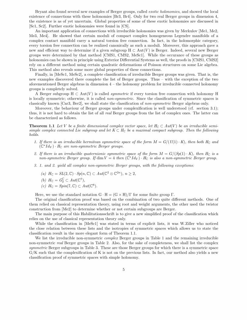
Bryant also found several new examples of Berger groups, called exotic holonomies, and showed the localexistence of connections with these holonomies [Br3, Br4]. Only for two real Berger groups in dimension 4,the existence is as of yet uncertain. Global properties of some of these exotic holonomies are discussed in[Sc1, Sc2]. Further exotic holonomies were found in [CS].

An important application of connections with irreducible holonomies was given by Merkulov [Me1, Me2,Me3, Me4]. He showed that certain moduli of compact complex homogeneous Legendre manifolds of acomplex contact manifold carry a natural torsion free connection. In fact, in the holomorphic category,every torsion free connection can be realized canonically as such a moduli. Moreover, this approach gave anew and efficient way to determine if a given subgroup H ⊂ Aut(V ) is Berger. Indeed, several new Bergergroups were determined by that method [CMS1, CMS2, MeSc1]. While the occurance of these groups asholonomies can be shown in principle using Exterior Differential Systems as well, the proofs in [CMS1, CMS2]rely on a different method using certain quadratic deformations of Poisson structures on some Lie algebra.This method also reveals some more global properties of these connections.

Finally, in [MeSc1, MeSc2], a complete classification of irreducible Berger groups was given. That is, thenew examples discovered there complete the list of Berger groups. Thus – with the exception of the twoaforementioned Berger algebras in dimension 4 – the holonomy problem for irreducible connected holonomygroups is completely solved.

A Berger subgroup H ⊂ Aut(V ) is called symmetric if every torsion free connection with holonomy His locally symmetric; otherwise, it is called non-symmetric. Since the classification of symmetric spaces isclassically known [Car3, Ber2], we shall state the classification of non-symmetric Berger algebras only.

Moreover, the behaviour of Berger groups under complexification is well understood (cf. section 3.1);thus, it is not hard to obtain the list of all real Berger groups from the list of complex ones. The latter canbe characterized as follows.

Theorem 1.1 Let V be a finite dimensional complex vector space, let HC ⊂ Aut(V ) be an irreducible semi-simple complex connected Lie subgroup and let K ⊂ HC be a maximal compact subgroup. Then the followingholds.

1. If there is an irreducible hermitean symmetric space of the form M = G/(U(1) ·K), then both HC and(C∗IdV ) ·HC are non-symmetric Berger groups.

2. If there is an irreducible quaternionic symmetric space of the form M = G/(Sp(1) · K), then HC is anon-symmetric Berger group. If dimV = 4 then (C∗IdV ) ·HC is also a non-symmetric Berger group.

3. 1. and 2. yield all complex non-symmetric Berger groups, with the following exceptions:

(a) HC = SL(2,C) · Sp(n,C) ⊂ Aut(C2 ⊗ C2n), n ≥ 2,

(b) HC = GC

2 ⊂ Aut(C7),

(c) HC = Spin(7,C) ⊂ Aut(C8).

Here, we use the standard notation G ·H = (G×H)/Γ for some finite group Γ.The original classification proof was based on the combination of two quite different methods. One of

them relied on classical representation theory, using root and weight arguments, the other used the twistorconstruction from [Me2] to determine whether or not certain subgroups are Berger.

The main purpose of this Habilitationsschrift is to give a new simplified proof of the classification whichrelies on the use of classical representation theory only.

While the classification in [MeSc1] was stated in terms of explicit lists, it was W.Ziller who noticedthe close relation between these lists and the isotropies of symmetric spaces which allows us to state theclassification result in the more elegant form of Theorem 1.1.

We list the irreducible non-symmetric complex Berger groups in Table 1 and the remaining irreduciblenon-symmetric real Berger groups in Table 2. Also, for the sake of completeness, we shall list the complexsymmetric Berger subgroups in Table 3. These are those Berger groups for which there is a symmetric spaceG/K such that the complexification of K is not on the previous lists. In fact, our method also yields a newclassification proof of symmetric spaces with simple holonomy.

5

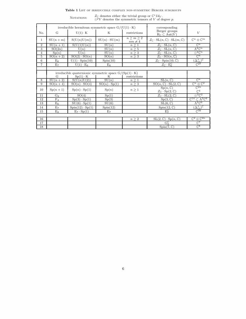
Table 1 List of irreducible complex non-symmetric Berger subgroups

Notations:ZC denotes either the trivial group or C∗IdV .⊙pV denotes the symmetric tensors of V of degree p.

irreducible hermitean symmetric space G/(U(1) · K) corresponding

No. G U(1)· K K restrictionsBerger groupsHC ⊂ Aut(V ) V

1 SU(n + m) S(U(n)U(m)) SU(n) · SU(m)n ≥ m ≥ 2

nm 6= 4ZC · SL(n, C) · SL(m, C) Cn ⊗ Cm

2 SU(n + 1) S(U(1)U(n)) SU(n) n ≥ 1 ZC · SL(n, C) Cn

3 SO(2n) U(n) SU(n) n ≥ 5 ZC · SL(n, C) Λ2Cn

4 Sp(n) U(n) SU(n) n ≥ 3 ZC · SL(n, C) ⊙2Cn

5 SO(n + 2) SO(2) · SO(n) SO(n) n ≥ 3 ZC · SO(n, C) Cn

6 E6 U(1) · Spin(10) Spin(10) ZC · Spin(10, C) (∆+10)C

7 E7 U(1) · E6 E6 ZC · EC6 C27

irreducible quaternionic symmetric space G/(Sp(1) · K)G Sp(1) · K K restrictions

8 SU(n + 2) S(U(n)U(2)) SU(n) n ≥ 1 SL(n, C) Cn

9 SO(n + 4) SO(n) · SO(4) SO(n) · Sp(1) n ≥ 3 SO(n, C) · SL(2, C) Cn ⊗ C2

10 Sp(n + 1) Sp(n) · Sp(1) Sp(n) n ≥ 1Sp(n, C)

ZC · Sp(2, C)C2n

C4

11 G2 SO(4) Sp(1) ZC · SL(2, C) ⊙3C2

12 F4 Sp(3) · Sp(1) Sp(3) Sp(3, C) C14 ⊂ Λ3C6

13 E6 SU(6) · Sp(1) SU(6) SL(6, C) Λ3C6

14 E7 Spin(12) · Sp(1) Spin(12) Spin(12, C) (∆+12)C

15 E8 E7 · Sp(1) E7 EC7 C56

16 n ≥ 2 SL(2, C) · Sp(n, C) C2 ⊗ C2n

17 GC2 C7

18 Spin(7, C) C8

6

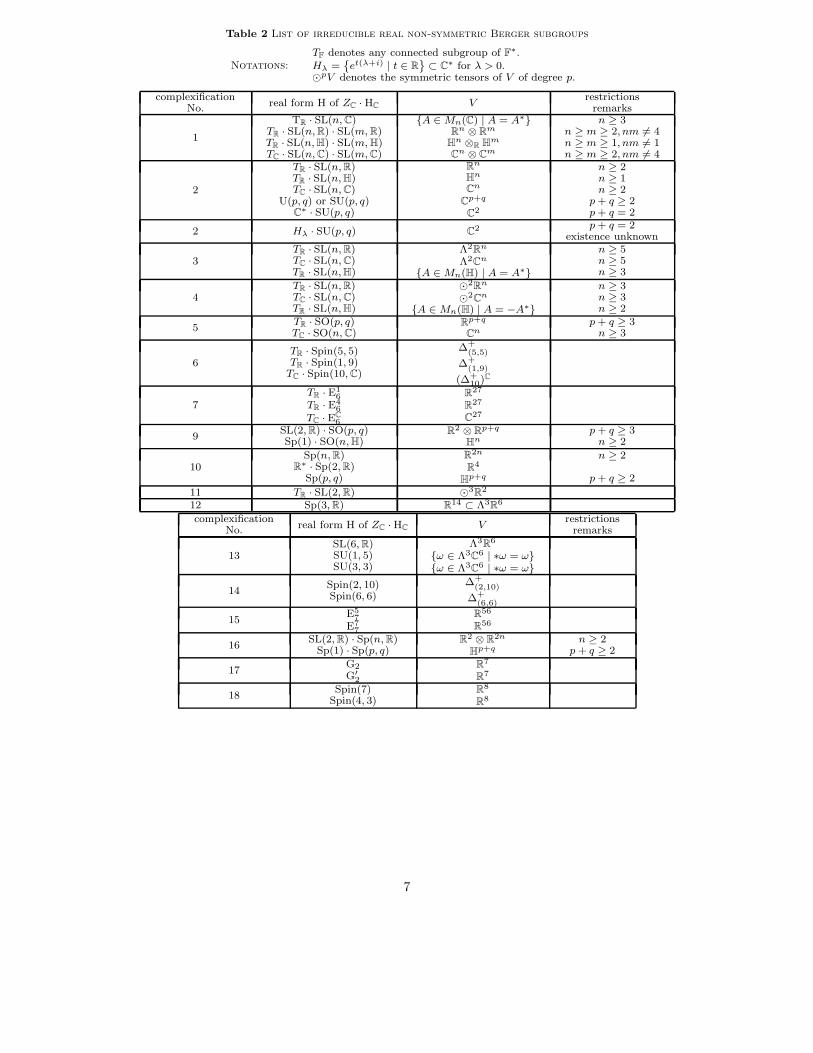
Table 2 List of irreducible real non-symmetric Berger subgroups

Notations:TF denotes any connected subgroup of F∗.Hλ =

˘

et(λ+i) | t ∈ R¯

⊂ C∗ for λ > 0.⊙pV denotes the symmetric tensors of V of degree p.

complexificationNo. real form H of ZC · HC V

restrictionsremarks

1

TR · SL(n, C)TR · SL(n, R) · SL(m, R)TR · SL(n, H) · SL(m, H)TC · SL(n, C) · SL(m, C)

A ∈ Mn(C) | A = A∗Rn ⊗ Rm

Hn ⊗R Hm

Cn ⊗ Cm

n ≥ 3n ≥ m ≥ 2, nm 6= 4n ≥ m ≥ 1, nm 6= 1n ≥ m ≥ 2, nm 6= 4

2

TR · SL(n, R)TR · SL(n, H)TC · SL(n, C)

U(p, q) or SU(p, q)C∗ · SU(p, q)

Rn

Hn

Cn

Cp+q

C2

n ≥ 2n ≥ 1n ≥ 2

p + q ≥ 2p + q = 2

2 Hλ · SU(p, q) C2 p + q = 2existence unknown

3TR · SL(n, R)TC · SL(n, C)TR · SL(n, H)

Λ2Rn

Λ2Cn

A ∈ Mn(H) | A = A∗

n ≥ 5n ≥ 5n ≥ 3

4TR · SL(n, R)TC · SL(n, C)TR · SL(n, H)

⊙2Rn

⊙2Cn

A ∈ Mn(H) | A = −A∗

n ≥ 3n ≥ 3n ≥ 2

5TR · SO(p, q)TC · SO(n, C)

Rp+q

Cnp + q ≥ 3

n ≥ 3

6TR · Spin(5, 5)TR · Spin(1, 9)

TC · Spin(10, C)

∆+(5,5)

∆+(1,9)

(∆+10)C

7TR · E1

6TR · E4

6TC · EC

6

R27

R27

C27

9SL(2, R) · SO(p, q)Sp(1) · SO(n, H)

R2 ⊗ Rp+q

Hnp + q ≥ 3

n ≥ 2

10Sp(n, R)

R∗ · Sp(2, R)Sp(p, q)

R2n

R4

Hp+q

n ≥ 2

p + q ≥ 2

11 TR · SL(2, R) ⊙3R2

12 Sp(3, R) R14 ⊂ Λ3R6

complexificationNo. real form H of ZC · HC V

restrictionsremarks

13SL(6, R)SU(1, 5)SU(3, 3)

Λ3R6

ω ∈ Λ3C6 | ∗ω = ωω ∈ Λ3C6 | ∗ω = ω

14Spin(2, 10)Spin(6, 6)

∆+(2,10)

∆+(6,6)

15E5

7E7

7

R56

R56

16SL(2, R) · Sp(n, R)

Sp(1) · Sp(p, q)R2 ⊗ R2n

Hp+qn ≥ 2

p + q ≥ 2

17G2

G′2

R7

R7

18Spin(7)

Spin(4, 3)R8

R8

7

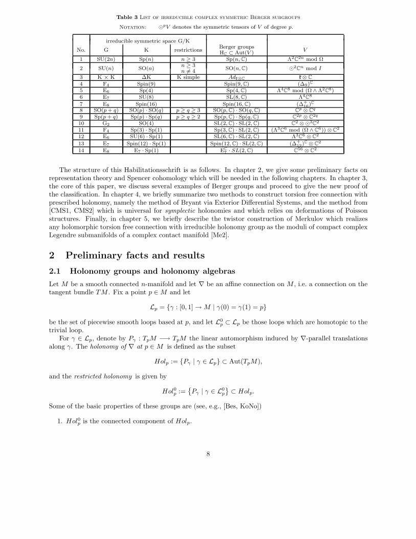
Table 3 List of irreducible complex symmetric Berger subgroups

Notation: ⊙pV denotes the symmetric tensors of V of degree p.

irreducible symmetric space G/K

No. G K restrictionsBerger groupsHC ⊂ Aut(V ) V

1 SU(2n) Sp(n) n ≥ 3 Sp(n, C) Λ2C2n mod Ω

2 SU(n) SO(n)n ≥ 3n 6= 4 SO(n, C) ⊙2Cn mod I

3 K × K ∆K K simple Adk⊗C k⊗ C

4 F4 Spin(9) Spin(9, C) (∆9)C

5 E6 Sp(4) Sp(4, C) Λ4C8 mod (Ω ∧ Λ2C8)6 E7 SU(8) SL(8, C) Λ4C8

7 E8 Spin(16) Spin(16, C) (∆+16)C

8 SO(p + q) SO(p) · SO(q) p ≥ q ≥ 3 SO(p, C) · SO(q, C) Cp ⊗ Cq

9 Sp(p + q) Sp(p) · Sp(q) p ≥ q ≥ 2 Sp(p, C) · Sp(q, C) C2p ⊗ C2q

10 G2 SO(4) SL(2, C) · SL(2, C) C2 ⊗⊙3C2

11 F4 Sp(3) · Sp(1) Sp(3, C) · SL(2, C) (Λ3C6 mod (Ω ∧ C6)) ⊗ C2

12 E6 SU(6) · Sp(1) SL(6, C) · SL(2, C) Λ3C6 ⊗ C2

13 E7 Spin(12) · Sp(1) Spin(12, C) · SL(2, C) (∆+12)C ⊗ C2

14 E8 E7 · Sp(1) EC7 · SL(2, C) C56 ⊗ C2

The structure of this Habilitationsschrift is as follows. In chapter 2, we give some preliminary facts onrepresentation theory and Spencer cohomology which will be needed in the following chapters. In chapter 3,the core of this paper, we discuss several examples of Berger groups and proceed to give the new proof ofthe classification. In chapter 4, we briefly summarize two methods to construct torsion free connection withprescribed holonomy, namely the method of Bryant via Exterior Differential Systems, and the method from[CMS1, CMS2] which is universal for symplectic holonomies and which relies on deformations of Poissonstructures. Finally, in chapter 5, we briefly describe the twistor construction of Merkulov which realizesany holomorphic torsion free connection with irreducible holonomy group as the moduli of compact complexLegendre submanifolds of a complex contact manifold [Me2].

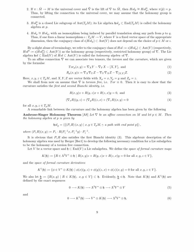
2 Preliminary facts and results

2.1 Holonomy groups and holonomy algebras

Let M be a smooth connected n-manifold and let ∇ be an affine connection on M , i.e. a connection on thetangent bundle TM . Fix a point p ∈M and let

Lp = γ : [0, 1]→M | γ(0) = γ(1) = p

be the set of piecewise smooth loops based at p, and let L0p ⊂ Lp be those loops which are homotopic to the

trivial loop.For γ ∈ Lp, denote by Pγ : TpM −→ TpM the linear automorphism induced by ∇-parallel translations

along γ. The holonomy of ∇ at p ∈M is defined as the subset

Holp := Pγ | γ ∈ Lp ⊂ Aut(TpM),

and the restricted holonomy is given by

Hol0p :=

Pγ | γ ∈ L0p

⊂ Holp.

Some of the basic properties of these groups are (see, e.g., [Bes, KoNo])

1. Hol0p is the connected component of Holp.

8

2. If π : M → M is the universal cover and ∇ is the lift of ∇ to M , then Holp ∼= Hol0p, where π(p) = p.Thus, by lifting the connection to the universal cover, we may assume that the holonomy group isconnected.

3. Hol0p is a closed Lie subgroup of Aut(TpM); its Lie algebra holp ⊂ End(TpM) is called the holonomyalgebra at p.

4. Holp ∼= Holq, with an isomorphism being induced by parallel translation along any path from p to q.Thus, if one fixes a linear isomorphism ı : TpM → V , where V is a fixed vector space of the appropriatedimension, then the conjugacy class of ı(Holp) ⊂ Aut(V ) does not depend on the choice of p ∈M or ı.

By a slight abuse of terminology, we refer to the conjugacy class ofHol := ı(Holp) ⊂ Aut(V ) (respectively,Hol0 := ı(Hol0p) ⊂ Aut(V )) as the holonomy group (respectively, restricted holonomy group) of ∇. The Liealgebra hol ⊂ End(V ) of Hol ⊂ Aut(V ) is called the holonomy algebra of ∇.

To an affine connection ∇ we can associate two tensors, the torsion and the curvature, which are givenby the formulae

Torp(x, y) = ∇XY −∇Y X − [X,Y ], and (1)

Rp(x, y)z = ∇X∇Y Z −∇Y∇XZ −∇[X,Y ]Z. (2)

Here, x, y, z ∈ TpM , and X,Y, Z are vector fields with Xp = x, Yp = y and Zp = z.We shall from now on assume that ∇ is torsion free, i.e. Tor ≡ 0. Then it is easy to show that the

curvature satisfies the first and second Bianchi identity, i.e.

R(x, y)z +R(y, z)x+R(z, x)y = 0, and (3)

(∇xR)(y, z) + (∇yR)(z, x) + (∇zR)(x, y) = 0 (4)

for all x, y, z ∈ TpM .A remarkable link between the curvature and the holonomy algebra has been given by the following

Ambrose-Singer Holonomy Theorem [AS] Let ∇ be an affine connection on M and let p ∈ M . Thenthe holonomy algebra at p is given by

holp = 〈(PγR) (x, y) | x, y ∈ TpM,γ a path with end point p〉 ,

where (PγR)(x, y) := Pγ · R(P−1γ x, P−1

γ y) · P−1γ .

It is obvious that PγR also satisfies the first Bianchi identity (3). This algebraic description of theholonomy algebra was used by Berger [Ber1] to develop the following necessary condition for a Lie subalgebrato be the holonomy of a torsion free connection.

Let V be a vector space and h ⊂ End(V ) a Lie subalgebra. We define the space of formal curvature maps

K(h) := R ∈ Λ2V ∗ ⊗ h | R(x, y)z +R(y, z)x+R(z, x)y = 0 for all x, y, z ∈ V ,

and the space of formal curvature derivatives

K1(h) := φ ∈ V ∗ ⊗K(h) | φ(x)(y, z) + φ(y)(z, x) + φ(z)(x, y) = 0 for all x, y, z ∈ V .

We also let h := R(x, y) | R ∈ K(h), x, y ∈ V ⊂ h. Evidently, h ⊳ h. Note that K(h) and K1(h) aredefined by the exact sequences

0 −→ K(h) −→ Λ2V ∗ ⊗ h −→ Λ3V ∗ ⊗ V (5)

and0 −→ K1(h) −→ V ∗ ⊗K(h) −→ Λ3V ∗ ⊗ h, (6)

9

where in each case, the last map is given by the composition of the natural inclusion and the skew-symmetrization map, i.e. Λ2V ∗ ⊗ h → Λ2V ∗ ⊗ V ∗ ⊗ V → Λ3V ∗ ⊗ V in the first and V ∗ ⊗ K(h) →V ∗ ⊗ Λ2V ∗ ⊗ h→ Λ3V ∗ ⊗ h in the second case.

From (3) it follows that PγR ∈ K(holp) for all path γ with end point p; hence the Ambrose-SingerHolonomy Theorem implies that hol

p= holp. Moreover, from (4) it follows that the map x 7→ ∇xR lies

in K1(holp). Thus, if K1(holp) = 0 then ∇R ≡ 0, i.e. the connection is locally symmetric. These factsmotivate the following definition.

Definition 2.1 An irreducible Lie subalgebra h ⊂ End(V ) is called a Berger algebra if h = h. A Berger

algebra h ⊂ End(V ) is called symmetric if K1(h) = 0 and non-symmetric otherwise.A Lie subgroup H ⊂ Aut(V ) is called a (symmetric respectively non-symmetric) Berger group if its Lie

algebra h ⊂ End(V ) is a (symmetric respectively non-symmetric) Berger algebra.

In the literature, the two criteria for a non-symmetric Berger algebra are usually referred to as Berger’sfirst and second criterion. Our discussion from above now yields the following.

Proposition 2.2 [Ber1] Let H ⊂ Aut(V ) be an irreducible Lie subgroup which occurs as the holonomy groupof a torsion free affine connection on some manifold M . Then H must be a Berger group. If the connectionis not locally symmetric, then H must be a non-symmetric Berger group.

We shall often utilize the following simple

Lemma 2.3 If h ⊂ End(V ) is an irreducible Berger algebra, and if K(h) is a trivial h-module, then h issymmetric.

Proof. W.l.o.g. we may assume that dimV > 2. Suppose K(h) is a trivial h-module. Then K1(h) ⊂V ∗ ⊗ K(h) is a submodule and thus, since V is irreducible, we have K1(h) = V ∗ ⊗W for some subspaceW ⊂ K(h). Suppose there is a 0 6= R ∈ W . Pick independent elements x, y, z ∈ V such that R(x, y) 6= 0,and define φ : V → W such that φ(x) = φ(y) = 0 and φ(z) = R. Then it follows that φ /∈ K1(h) which is acontradiction.

Therefore, W = 0, i.e. K1(h) = 0, and thus h is symmetric.

2.2 Spencer cohomology

We shall briefly summarize the construction of the Spencer complex for a Lie subalgebra h ⊂ End(V ). Fora more detailed exposition, we refer the interested reader to [G, O] and [Br4].

Let V be a finite dimensional vector space over F. We let Ap,q(V ) := ⊙pV ∗ ⊗ ΛqV ∗. This spacecan be thought of as the space of q-forms on V with values in the space of homogeneous polynomialson V of degree p. Exterior differentiation thus yields a map δ : Ap,q(V ) → Ap−1,q+1(V ), which makesA∗,∗(V ) =

⊕

p,q≥0Ap,q(V ) into a bigraded complex. Likewise,

⊕

p,q≥0(V ⊗ Ap,q(V )) becomes a bigraded

complex by the maps δV := IdV ⊗ δ.Let h ⊂ End(V ) ∼= V ∗ ⊗ V be a subalgebra. The k-th prolongation of h, denoted by h(k) for an integer

k, is defined by the formulae h(−1) = V , h(0) = h, and

h(k) = δ−1V (h(k−1) ⊗ V ∗).

That is,h(k) = (h⊗⊙kV ∗) ∩ (V ⊗⊙k+1V ∗),

where we use exterior differentiation δ : ⊙k+1V ∗ → V ∗ ⊗⊙kV ∗ to regard both h ⊗⊙kV ∗ and V ⊗⊙k+1V ∗

as subspaces of V ⊗ V ∗ ⊗⊙kV ∗. For example,

h(1) = α ∈ V ∗ ⊗ h | α(x)y = α(y)x for all x, y ∈ V .

10

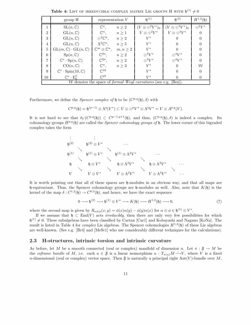
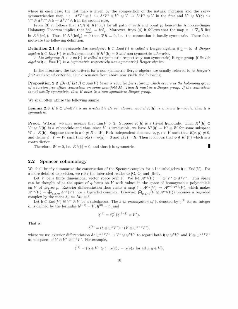
Table 4: List of irreducible complex matrix Lie groups H with h(1) 6= 0

group H representation V h(1) h(2) H1,2(h)

1 SL(n,C) Cn, n ≥ 2 (V ⊗⊙2V ∗)0 (V ⊗⊙3V ∗)0 ⊙2V ∗

2 GL(n,C) Cn, n ≥ 1 V ⊗⊙2V ∗ V ⊗⊙3V ∗ 0

3 GL(n,C) ⊙2Cn, n ≥ 2 V ∗ 0 0

4 GL(n,C) Λ2C

n, n ≥ 5 V ∗ 0 0

5 GL(m,C) ·GL(n,C) Cm ⊗ Cn, m,n ≥ 2 V ∗ 0 0

6 Sp(n,C) C2n, n ≥ 2 ⊙3V ∗ ⊙4V ∗ 0

7 C∗ · Sp(n,C) C

2n, n ≥ 2 ⊙3V ∗ ⊙4V ∗ 0

8 CO(n,C) Cn, n ≥ 3 V ∗ 0 W

9 C∗ · Spin(10,C) C16 V ∗ 0 0

10 C∗ · EC

6 C27 V ∗ 0 0W denotes the space of formal Weyl curvatures (see e.g. [Bes]).

Furthermore, we define the Spencer complex of h to be (Cp,q(h), δ) with

Cp,q(h) = h(p−1) ⊗ Λq(V ∗) ⊂ V ⊗⊙pV ∗ ⊗ ΛqV ∗ = V ⊗Ap,q(V ).

It is not hard to see that δV (Cp,q(h)) ⊂ Cp−1,q+1(h), and thus, (Cp,q(h), δ) is indeed a complex. Itscohomology groups Hp,q(h) are called the Spencer cohomology groups of h. The lower corner of this bigradedcomplex takes the form

......

h(2) h(2) ⊗ V ∗ · · ·ց ց

h(1) h(1) ⊗ V ∗ h(1) ⊗ Λ2V ∗ · · ·ց ց ց

h h⊗ V ∗ h⊗ Λ2V ∗ h⊗ Λ3V ∗ · · ·ց ց ց ց

V V ⊗ V ∗ V ⊗ Λ2V ∗ V ⊗ Λ3V ∗ · · ·

It is worth pointing out that all of these spaces are h-modules in an obvious way, and that all maps areh-equivariant. Thus, the Spencer cohomology groups are h-modules as well. Also, note that K(h) is thekernel of the map δ : C1,2(h)→ C0,3(h), and hence, we have the exact sequence

0 −→ h(2) −→ h(1) ⊗ V ∗ −→ K(h) −→ H1,2(h) −→ 0, (7)

where the second map is given by Rα⊗φ(x, y) = φ(x)α(y) − φ(y)α(x) for α⊗ φ ∈ h(1) ⊗ V ∗.If we assume that h ⊂ End(V ) acts irreducibly, then there are only very few possibilities for which

h(1) 6= 0. These subalgebras have been classified by Cartan [Car1] and Kobayashi and Nagano [KoNa]. Theresult is listed in Table 4 for complex Lie algebras. The Spencer cohomologies H1,2(h) of these Lie algebrasare well-known. (See e.g. [Br4] and [MeSc1] who use considerably different techniques for the calculations).

2.3 H-structures, intrinsic torsion and intrinsic curvature

As before, let M be a smooth connected (real or complex) manifold of dimension n. Let π : F → M bethe coframe bundle of M , i.e. each u ∈ F is a linear isomorphism u : Tπ(u)M−→V , where V is a fixedn-dimensional (real or complex) vector space. Then F is naturally a principal right Aut(V )-bundle over M ,

11

where the right action Rg : F→ F is defined by Rg(u) = g−1 u. The tautological 1-form θ on F with valuesin V is defined by θ(ξ) = u(π∗(ξ)) for ξ ∈ TuF. For θ, we have the Aut(V )-equivariance

R∗g(θ) = g−1θ. (8)

Let H ⊂ Aut(V ) be a closed Lie subgroup and let h ⊂ End(V ) be the Lie algebra of H. An H-structure onM is, by definition, an H-subbundle F ⊂ F. For any H-structure, we will denote the restrictions of π and θto F by the same letters. Given A ∈ h we define the vector field A∗ on F by

(A∗)u =d

dt

(

Rexp(tA)(u))

|t=0.

The vector fields A∗ are called the fundamental vertical vector fields on F . It is evident that π∗(A∗) = 0and thus θ(A∗) = 0 for all A ∈ h; in fact, A∗ | A ∈ h = ker(π∗). Moreover, for A,B ∈ h we have[A∗, B∗] = [A,B]∗.

For a given H-structure π : F →M , we define the vector bundles h(k)F := F ×H h(k), Cp,q

F := F ×HCp,q(h)

and Hp,qF := F ×H Hp,q(h). Note that hF := h

(0)F is a subbundle of T ∗M ⊗ TM , and that h−1

F = TM . The

boundary maps of the Spencer complex induce bundle maps δp,qF : Cp,q

F → Cp−1,q+1F whose kernels we denote

by Zp,qF . In particular, we let K(hF ) := Z1,2

F .A connection on F is a h-valued 1-form ω on F satisfying the conditions

ω(A∗) = A for all A ∈ h, andR∗

h(ω) = h−1ωh for all h ∈ H.(9)

Given a connection ω, its torsion Θ is the V -valued 2-form given by

Θ = dθ + ω ∧ θ. (10)

From (8), (9) and (10) it follows thatR∗

hΘ = h−1Θ, (11)

and hence, Θ induces a section Tor of the bundle Z0,2F = Λ2T ∗M ⊗ TM . Note that Tor coincides with the

torsion tensor given in (1). ω is called torsion free if Θ = 0. Using the natural projection map p : Z0,2F → H0,2

F ,

we obtain a section τ := p(Θ) of H0,2F .

Now let ω′ be another connection on F with torsion Θ′. From (9) it follows that α := ω′ − ω is anh-valued 1-form with α(A∗) = 0 and R∗

hα = h−1αh, and hence, α induces a section α of hF ⊗ T ∗M . Note

that the section δ1,1F (α) of Z0,2

F = Λ2T ∗M ⊗ TM is induced by the section α ∧ θ. But for the torsion, we

have Θ′ = Θ + α ∧ θ, and hence p(Θ−Θ′) = p(δ1,1F (α)) = 0, i.e. the section τ = p(Θ) is independent of the

choice of ω. This motivates the following terminology.

Definition 2.4 Let π : F → M be an H-structure. Then the vector bundle H0,2F is called the intrinsic

torsion bundle of F , and the section τ of H0,2F defined by any connection is called the intrinsic torsion of F .

Moreover, F is called torsion free or 1-flat if its intrinsic torsion τ vanishes.

It is then obvious that F admits a torsion free connection iff F is torsion free, and moreover, that the

difference of two torsion free connections is given by a section of h(1)F . In particular, if h(1) = 0 then F admits

at most one torsion free connection.Suppose now that F is torsion free and let ω be a torsion free connection on F , i.e.

dθ + ω ∧ θ = 0.

Exterior differentiation yields the first Bianchi identity

Ω ∧ θ = 0, (12)

12

whereΩ := dω + ω ∧ ω

is the curvature 2-form of ω. Then R∗hΩ = h−1Ωh for all h ∈ H , and hence Ω induces a section R of

Λ2T ∗M ⊗ hF . Note that R coincides with the curvature tensor given in (2). Moreover, (12) implies thatδ1,2(R) = 0. Therefore, R is a section of K(hF ) = Z1,2

F and thus induces a section ρ := p(R) of H1,2F where

again, p : K(hF )→ H1,2F is the natural projection.

Now let ω′ be another torsion free connection on F , i.e. α := ω − ω′ satisfies α ∧ θ = 0 or, equivalently,the induced section α of T ∗M ⊗ hF satisies δ1,1(α) = 0. If we denote the curvature sections of ω and ω′ byR and R′ respectively, then an easy calculation shows that

R′ = R+ dα+ α ∧ α.

It is now straightforward to verify that the map

φ : TM −→ h(1)

X 7−→ ∇Xα+ α(X)α(13)

is well defined and satisfiesδ2,1(φ) = dα+ α ∧ α, (14)

and thus the section ρ := pr(R) of H1,2F is independent of the choice of the torsion free connection.

Definition 2.5 Let π : F →M be a torsion free H-structure. The section ρ of H1,2F defined above is called

the intrinsic curvature of F . Moreover, if ρ ≡ 0 then F is called 2-flat. F is called locally flat if there existsa torsion free connection on F whose curvature vanishes.

Evidently, local flatness implies 2-flatness. The converse is not true in general; indeed, F is 2-flat iff forany p ∈M , there exists a torsion free connection on F whose curvature vanishes at p.

In general, an H-structure F is called k-flat if for every p ∈ M there is a torsion free connection on Fwhose curvature vanishes at p up to (k − 1)-st order. One can show that the obstruction for F to be k-flat

is represented by a section of Hk,2F . We shall not give the precise definition, but refer the interested reader

to [Br2] for details.

2.4 A brief review of representation theory

In this section, we shall give a brief outline of standard facts of representation theory of complex semi-simpleLie algebras. For a more detailed exposition, see e.g. [FH] or [Hu].

Let g be a semi-simple complex Lie algebra and G the associated simply connected Lie group, and lett ⊂ g be a Cartan subalgebra, i.e. a maximal abelian self-normalizing subalgebra. The rank of g is bydefinition rk(g) := dim t.

If ρ : g → End(V ) is a representation of g on a complex vector space V , then for any λ ∈ t∗ we definethe weight space Vλ by

Vλ = v ∈ V | ρ(h)v = λ(h)v for all h ∈ t.

An element λ ∈ t∗ is called a weight of V if Vλ 6= 0. We let Φ ⊂ t∗ be the set of weights of ρ, and thus havethe decomposition

V =⊕

λ∈Φ

Vλ.

In particular, if V = g and ρ is the adjoint representation, then we get the Cartan decomposition

g = t⊕⊕

α∈∆

gα,

i.e. t is the weight space of weight 0, and ∆ ⊂ t∗ is the set of non-zero weights. ∆ is called the set of rootsor the root system of g. It is well known that dim gα = 1 for all α ∈ ∆.

13

For each root system ∆, there is a subset S = α1, . . . , αr ⊂ ∆ where r = rk(g), called a system ofsimple roots, with the property that every α ∈ ∆ may be expressed as a linear combination α =

∑ri=1 aiαi

with either ai ≥ 0 for all i, or ai ≤ 0 for all i. Then α is called a positive respectively a negative root, andthe sets of positive and negative roots are denoted by ∆±. Thus, ∆ = ∆+ ∪∆−.

For any root α ∈ ∆, there is a unique element Hα ∈ [gα, g−α] ⊂ t such that α(Hα) = 2. If S =α1, . . . , αr is the set of simple roots, then the associated set Hα1

, . . . , Hαr forms a basis of t. Its dual

basis λ1, . . . , λr of t∗ is called the set of fundamental weights. The lattice Λ ⊂ t∗ generated by this basisis called the (integral) weight lattice. It is well known that Φ ⊂ Λ for any representation ρ. The lattice Πgenerated by ∆ is called the root lattice. Evidently, Π ⊂ Λ, and moreover, the quotient Λ/Π is isomorphicto the center of the simply connected Lie group G associated to g.

Let Λ+ := λ ∈ Λ | λ =∑r

i=1 aiλi with ai ≥ 0 be the set of dominant weights. Note that ai = λi(Hαi).

If ρ : g → End(V ) is an irreducible representation then there exists a unique weight λ0 ∈ Λ+, called thedominant weight of ρ, such that dimVλ0

= 1 and ρ(gα)Vλ0= 0 for all α ∈ ∆+. Any non-zero element of Vλ0

is called a dominant weight vector. In fact, the dominant weight determines the representation ρ, and thusestablishes a one-to-one correspondence between finite-dimensional irreducible representations of g and theset Λ+.

Given an λ ∈ Λ and a root α, we let

〈λ, α〉 := λ(Hα) ∈ Z.

Note that 〈 , 〉 is linear in the first entry only. There is a ad(g)-invariant symmetric bilinear form B on g,the so-called Killing form, which is given by B(x, y) := tr(adx ady) for all x, y ∈ g. We shall use it toidentify g and g∗. With this, we have

〈λ, α〉 =2B(λ, α)

B(α, α). (15)

The significance of 〈λ, α〉 is the following. If λ occurs as the weight of an irreducible representation of g and〈λ, α〉 > 0 (〈λ, α〉 < 0, respectively) then λ−kα (λ+kα, respectively) is also a weight of that representationfor k = 1, . . . , | 〈λ, α〉 |.

For any root α ∈ ∆, denote by σα the orthogonal reflection of t∗ in the hyperplane perpendicular to α.The Weyl group W of g is the group generated by all σα. W is always finite. If g is simple then W actsirreducibly on t∗. Moreover, W acts transitively on the set of roots of equal length, and the set of weightsΦ of any irreducible representation is W -invariant.

A weight λ ∈ Φ of an irreducible representation ρ : g→ End(V ) is called extremal if it lies in the W -orbitof the dominant weight. Two weights λ, µ ∈ Φ are said to have opposite sign if for all roots α we have〈λ, α〉 〈µ, α〉 ≤ 0. It is known that for every extremal weight λ there is always an extremal weight µ ofopposite sign.

For any two simple roots αi, αj ∈ S, it turns out that 〈αi, αj〉 ≤ 0. To a simple basis S, we associate theDynkin diagram of g by representing each αi ∈ S as a node, and to join the nodes of αi and αj by | 〈αi, αj〉 |edges. If | 〈αi, αj〉 | > 1 then αi, αj have different lengths, and we draw an arrow from the longer to theshorter root.

Any integral weight λ of g can be graphically represented by inscribing the integer 〈λ, αi〉 over the nodeof the Dynkin diagram corresponding to αi. In particular, we can represent any irreducible representation ρof g by inscribing the integers of the dominant weight on the nodes of the Dynkin diagram of g.

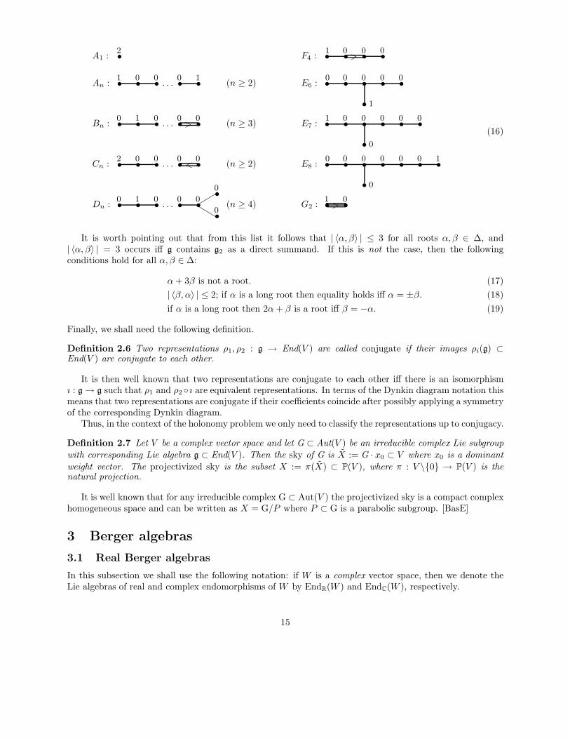
If g is simple, then the adjoint representation ρ : g→ End(g) is irreducible. Its dominant weight is calledthe maximal root of g. The following is the list of all Dynkin diagrams of simple Lie algebras, together withtheir maximal roots:

14

A1 : s2

F4 : s s s s>1 0 0 0

An : . . .s s s s s1 0 0 0 1

(n ≥ 2) E6 : s s s s s

s

0 0 0 0 0

1

Bn : . . .s s s s> s0 1 0 0 0

(n ≥ 3) E7 : s s s s s s

s

1 0 0 0 0 0

0

Cn : . . .ss s s< s2 0 0 0 0

(n ≥ 2) E8 : s s s s s s s

s

0 0 0 0 0 0 1

0

Dn : . . .s s s s s

s

s

0 1 0 0 0

0

0bb

""

(n ≥ 4) G2 : ss>1 0

(16)

It is worth pointing out that from this list it follows that | 〈α, β〉 | ≤ 3 for all roots α, β ∈ ∆, and| 〈α, β〉 | = 3 occurs iff g contains g2 as a direct summand. If this is not the case, then the followingconditions hold for all α, β ∈ ∆:

α+ 3β is not a root. (17)

| 〈β, α〉 | ≤ 2; if α is a long root then equality holds iff α = ±β. (18)

if α is a long root then 2α+ β is a root iff β = −α. (19)

Finally, we shall need the following definition.

Definition 2.6 Two representations ρ1, ρ2 : g → End(V ) are called conjugate if their images ρi(g) ⊂End(V ) are conjugate to each other.

It is then well known that two representations are conjugate to each other iff there is an isomorphismı : g→ g such that ρ1 and ρ2 ı are equivalent representations. In terms of the Dynkin diagram notation thismeans that two representations are conjugate if their coefficients coincide after possibly applying a symmetryof the corresponding Dynkin diagram.

Thus, in the context of the holonomy problem we only need to classify the representations up to conjugacy.

Definition 2.7 Let V be a complex vector space and let G ⊂ Aut(V ) be an irreducible complex Lie subgroup

with corresponding Lie algebra g ⊂ End(V ). Then the sky of G is X := G · x0 ⊂ V where x0 is a dominant

weight vector. The projectivized sky is the subset X := π(X) ⊂ P(V ), where π : V \0 → P(V ) is thenatural projection.

It is well known that for any irreducible complex G ⊂ Aut(V ) the projectivized sky is a compact complexhomogeneous space and can be written as X = G/P where P ⊂ G is a parabolic subgroup. [BasE]

3 Berger algebras

3.1 Real Berger algebras

In this subsection we shall use the following notation: if W is a complex vector space, then we denote theLie algebras of real and complex endomorphisms of W by EndR(W ) and EndC(W ), respectively.

15

Let V be a finite dimensional real vector space, and let h ⊂ EndR(V ) be a real Lie subalgebra. Wedenote their complexifications by VC := V ⊗R C and hC := h⊗R C. Then obviously, hC ⊂ EndC(VC), and bycomplexifying the exact sequences (5) and (6), we obtain

K(hC) = K(h)⊗R C and K1(hC) = K1(h)⊗R C.

In particular, h ⊂ EndR(V ) is a (symmetric respectively non-symmetric) Berger algebra iff hC ⊂ EndC(VC)is.

Let us now assume that h ⊂ EndR(V ) is irreducible. Then there are two cases to be distinguished.First, suppose that h is of real type, i.e. there is no complex structure on V which commutes with the

elements of h. This happens iff hC ⊂ EndC(VC) is also irreducible.Second, suppose that h is not of real type, i.e. there is a complex structure J on V which commutes

with the elements of h. That is, h ⊂ EndC(V ) w.r.t. this complex structure J . In this case, VC = W ⊕Wdecomposes into two irreducible hC-submodules of equal dimension given by

W = x+ iJx | x ∈ V and W = x− iJx | x ∈ V .

Let h1 := A ∈ h | JA ∈ h. Then h1 ⊳ h, and J induces a complex Lie algebra structure on h1; (h1)C canbe written as the direct sum of complex Lie algebras (h1)C = h+

1 ⊕ h−1 with

h+1 = A+ iJA | A ∈ h1 and h−1 = A− iJA | A ∈ h1.

Let R ∈ K(hC). Then for u, v ∈ W and w ∈ W the first Bianchi identity implies that R(u, v)w = 0.Since this is true for all w ∈ W , it follows that R(u, v) ∈ h+

1 . On the other hand, the Bianchi identity foru, v, w ∈ W , implies that the restriction R : Λ2W → h+

1 ⊂ hC lies in K(h+1 |W ). Likewise, the restriction

R : Λ2W → h−1 lies in K(h−1 |W ).Next, for any R ∈ K(hC) the first Bianchi identity also implies that R(u, v)w = R(u,w)v for all u ∈ W ,

v, w ∈W . Thus, we have a mapW −→ (hC|W )(1), u 7−→ R(u, ).

If (hC|W )(1) = 0 then this implies that R(W,W ) = 0, and hence K(hC) = K(h+1 |W ) ⊕ K(h−1 |W ). But

then hC⊂ h+

1 ⊕ h−1 = (h1)C. Hence hC is not Berger unless h1 = h, i.e. h is a complex Lie algebra which actsirreducibly on the complex vector space V .

We define a map ı : hC → EndC(V ) by

ı(A+ iB) := A+ JB. (20)

In fact, it is easy to see that ı(hC) ⊂ EndC(V ) is congruent to (hC)|W ⊂ EndC(W ), and hence (hC|W )(1) = 0iff (ı(hC))(1) = 0. Thus, we obtain the following.

Proposition 3.1 Let V be a finite dimensional real vector space, and let h ⊂ EndR(V ) be an irreducible realsubalgebra with complexification hC ⊂ EndC(VC).

1. If h is of real type, i.e. if there is no complex structure on V which commutes with the elements of h,then h is a Berger algebra iff hC ⊂ EndC(VC) is an irreducible Berger algebra.

2. If h is not of real type, i.e. if there is a complex structure J on V which commutes with the elementsof h, and if the subalgebra ı(hC) ⊂ EndC(V ) given by (20) satisfies (ı(hC))(1) = 0, then h is a Bergeralgebra iff Jh = h and h ⊂ EndC(V ) is a complex irreducible Lie subalgebra.

Thus, in order to classify all Berger algebras we need to classify all irreducible complex Berger subalgebrashC ⊂ EndC(VC), add all their real forms of real type, and finally, to investigate the real forms of the entriesof Table 4.

16

3.2 Examples of Berger algebras

3.2.1 Conformal Lie algebras

Let (V, 〈 , 〉) be a real or complex vector space with the symmetric bilinear form 〈 , 〉, let so(V ) be the Liealgebra of endomorphisms preserving 〈 , 〉 and co(V ) := span(IdV , so(V )). We have so(V ) ∼= Λ2V , with anisomorphism given by

(x ∧ y) · z := 〈x, z〉 y − 〈y, z〉x.

We use 〈 , 〉 to identify V and V ∗. With this, an element of K(so(V )) may be regarded as a map R : Λ2V →Λ2V , and an easy calculation involving the first Bianchi identity shows that K(so(n,C)) is symmetric w.r.t.the inner product on Λ2V induced by 〈 , 〉, i.e. K(so(V )) ⊂ ⊙2so(V ) ⊂ Λ2V ⊗ so(V ). But the image of therestriction δ1,2 : ⊙2so(V )→ Λ3V ⊗ V equals Λ4V , and hence we have

K(so(V )) ∼= (⊙2Λ2V )/Λ4V.

We define the map τ : K(co(V )) → so(V ) by the equation tr(R(x, y)) = 〈τ(R)x, y〉 for all x, y ∈ V andR ∈ K(co(V )). Clearly, the kernel of τ is K(so(V )). Moreover, one checks that for each A ∈ so(V ), the map

RA(x, y) := 〈Ax, y〉 IdV +1

2(Ax ∧ y −Ay ∧ x)

lies in K(co(V )), and τ(RA) = nA. Therefore, τ is surjective, and if we let Kc(V ) := RA | A ∈ so(V ),then

K(co(V )) ∼= K(so(V ))⊕Kc(V ).

Proposition 3.2 Let h ⊂ so(V, 〈 , 〉) be a proper irreducible Lie subalgebra where V is an n-dimensionalvector space over F = R or C with n ≥ 3, n 6= 4. Then K(h⊕FIdV ) = K(h). In particular, h⊕ FIdV is nota Berger algebra.

For the proof, we shall need the following Lemma.

Lemma 3.3 Let g be a simple Lie algebra and let h ⊂ g be a proper semi-simple subalgebra. Moreover, letW ⊂ g be a linear subspace such that [h,W ] ⊂W and [h⊥,W ] ⊂ h. Then either W = 0 or W = h⊥ in whichcase (g, h) is an irreducible symmetric pair.

Proof. Let h+ v ∈W with h ∈ h and v ∈ h⊥, and let h′ ∈ h. Consider the map τ := ad(v) ad(h′) : g→ g.By definition of the Killing form, we have tr(τ) = B(v, h′) = 0. Clearly, τ(h) ⊂ h⊥, and hence tr(τ) = tr(σ)with σ = prh⊥ ad(v)|h⊥ ad(h′)|h⊥ and where prh⊥ : g→ h⊥ is the orthogonal projection. Now, for v′ ∈ h⊥,we have

σ(v′) = prh⊥([(h+ v)− h, [h′, v′]]) = −[h, [h′, v′]],

since [h + v, [h′, v′]] ∈ [W, h⊥] ⊂ h and [h, [h′, v′]] ∈ h⊥. Therefore, σ = −ad(h)|h⊥ ad(h′)|h⊥ , and thus,tr(σ) = −cBh(h, h′) for some constant c > 0 and where Bh is the Killing form on h. Thus, Bh(h, h′) = 0 forall h′ ∈ h, and hence h = 0, i.e. W ⊂ h⊥.

Suppose that W 6= 0. Then there is an h-invariant decomposition h⊥ = V1 ⊕ V2 such that 0 6= V1 ⊂ Wand V1 is irreducible. Thus, [V1, V2] ⊂ [W, h⊥] ⊂ h. On the other hand, for vi ∈ Vi and h ∈ h, we haveB([v1, v2], h) = B(v1, [v2, h]) = 0, since [v2, h] ∈ V2. Therefore, [V1, V2] = 0.

Also, [V1, V1] ⊂ [W, h⊥] ⊂ h, and from there it follows that [V1, V1]⊕V1 ⊳g. Since g is simple and V1 6= 0,

this implies that W = V1 = h⊥ is h-irreducible and [h⊥, h⊥] = h.

Proof of Proposition 3.2. We have K(h ⊕ FIdV ) ⊂ K(co(V )), and we let W ⊂ so(V ) be the imageof K(h ⊕ FIdV ) under the natural projection K(co(V )) → Kc(V ) ∼= so(V ). Clearly, W is h-invariant, i.e.[h,W ] ⊂W . We need to show that W = 0.

We identify Λ2V and so(V ) as before, and denote the induced inner product on Λ2V by ( , ). Thenevery R ∈ K(h⊕ FId) can be written as R(α) = (A,α)Id+ 1

2 [A,α] +R(α) for all α ∈ so(V ), where A ∈W ,R ∈ K(so(V )) ⊂ ⊙2so(V ) and where 1

2 [A,α] +R(α) ∈ h for all α ∈ so(V ).

17

Let α, β ∈ h⊥ ⊂ so(V ). Then since R ∈ ⊙2so(V ), we have 0 = (R(α), β) − (α,R(β)) = 12 (−([A,α], β) +

(α, [A, β])) = −([A,α], β), and hence, [h⊥,W ] ⊂ h.Since so(V ) is simple, Lemma 3.3 implies that either W = 0, or W = h⊥ and (so(V ), h) is a symmetric

pair. If the latter is the case, then the symmetric reflection map σ : so(V ) → so(V ) with σ|h = Idh andσ|h⊥ = −Idh⊥ is an automorphism of so(V ) of order 2. It is known that any such automorphism is of theform σ = Adg for some g ∈ O(V ). Since h acts irreducibly on V and σ|h = Idh, Schur’s Lemma implies thateither g = λIdV , some λ ∈ F, or V is real and g an orthogonal complex structure on V .

In the first case, σ = Idso(V ) and hence h = so(V ) which was excluded. In the second case, h = u(V, g) ⊂sp(V,Ω), where Ω(x, y) := 〈x, gy〉. But we shall see in the following section that h ⊂ sp(V,Ω) implies that

K(h⊕ FId) = K(h), thus W = 0.

3.2.2 Symplectic Lie algebras

Let Ω be a non-degenerate 2-form on V , let sp(V,Ω) be the Lie algebra of linear endomorphisms of Vpreserving Ω, and let csp(V,Ω) = span(IdV , sp(V,Ω)). We have sp(V,Ω) ∼= ⊙2V , with an isomorphism givenby

(xy) · z := Ω(x, z)y + Ω(y, z)x. (21)

We use Ω to identify V and V ∗.For h = sp(V,Ω), it is known that H1,2(h) = 0 [Br4, p.37], and hence the map h(1) ⊗ V ∗ → K(h) from

(7) is surjective. From Table 4 we see that K(sp(V,Ω)) ∼= (⊙3V ⊗ V )/ ⊙4 V , with an explicit isomorphismbeing induced by

⊙3V ⊗ V −→ K(sp(V,Ω))τ 7−→ Rτ ,

where Rτ is determined by Ω(Rτ (x, y)z, w) = τ(xzw, y) − τ(yzw, x).

Lemma 3.4 Let R ∈ K(csp(V,Ω)) be given by R(x, y) = ρ(x, y)IdV + R(x, y) for some ρ ∈ Λ2V ∗ andR ∈ Λ2V ∗ ⊗ sp(n,C). Then ρ ∧ Ω = 0.

If dimV ≥ 6 then K(csp(V,Ω)) = K(sp(V,Ω)) and hence, csp(V,Ω) is not a Berger algebra. If dimV = 4then K(csp(V,Ω)) = K(sp(V,Ω))⊕ (Λ2V )/Ω.

Proof. Let R ∈ K(csp(V,Ω)) be given as above, and let τ(x, y, z, w) := Ω(R(x, y)z, w) − Ω(R(x, y)w, z).Then τ(x, y, z, w) = 2ρ(x, y)Ω(z, w), and the first Bianchi identity implies that ρ ∧ Ω = 0 as claimed. Thesecond assertion follows immediately.

Finally, one verifies that for each ρ ∈ Λ2V ∗ with ρ ∧ Ω = 0, the element Rρ given by

Rρ(x, y) = 4ρ(x, y)IdV +R(x, y),

Ω(R(x, y)z, w) = ρ(x, z)Ω(y, w) + ρ(x,w)Ω(y, z)− ρ(y, z)Ω(x,w) − ρ(y, w)Ω(x, z),

lies in K(csp(V )), and this shows the last assertion.

Let h ⊂ sp(V,Ω) be an irreducible subalgebra. We define an h-equivariant map

: ⊙2V −→ h

by the equationB(x y,A) = Ω(Ax, y) for all x, y ∈ V and A ∈ h.

Now we get the following Lemma whose verification is straightforward.

18

Lemma 3.5 Suppose h ⊂ sp(V,Ω) is an irreducible Lie subalgebra for which the product satisfies theidentity

B(x y, z w)−B(x w, z y) = 2µΩ(x, z)Ω(y, w) + µ[Ω(x, y)Ω(z, w) − Ω(x,w)Ω(y, z)] (22)

for all x, y, z, w ∈ V and some constant µ. Then there is an injective map h → K(h) given by A 7→ RA with

RA(x, y) = 2µ Ω(x, y) A+ x (Ay)− y (Ax).

In particular, h is a Berger algebra.

Corollary 3.6 Let G/(SL(2,C)H) be an irreducible complexified quaternionic symmetric space, i.e. H ⊂Sp(n,C). Then the Lie algebra h of H satisfies (22), hence h is a Berger algebra and H is a Berger group.

Proof. The isotropy representation induces an irreducible imbedding sl(2,C) ⊕ h → sl(2,C) ⊕ sp(n,C) ⊂so(C2⊗C2n), where the inner product on C2⊗C2n is the tensor product of the symplectic forms on C2 andC2n, respectively.

Let R denote the curvature tensor of the symmetric space. Then R is isotropy invariant and hence of theform

R(e⊗ x, f ⊗ y) = c1 Ω(x, y) ef + c2 〈e, f〉 x y

for some non-zero constants c1, c2. Here, 〈 , 〉 and Ω denote the symplectic forms on C2 and C2n, respectively,and we use the identification sl(2,C) ∼= ⊙2C2 from (21).

It is now straightforward to verify that the first Bianchi identity for R implies (22) with µ = c1

c2.

Corollary 3.7 The images of the following representations are Berger subgroups:

Group H Representation space Group H Representation space

SL(2, R) R4≃ ⊙

3R

2 E57 R

56

SL(2, C) C4≃ ⊙

3C

2 E77 R

56

SL(2, R) · SO(p, q) R2(p+q), (p + q) ≥ 2 EC

7 C56

SL(2, C) · SO(n, C) C2n, n ≥ 3 Spin(2, 10) R

32

Sp(1)SO(n, H) Hn≃ R

4n, n ≥ 3 Spin(6, 6) R32

Sp(3, R) R20

≃ Λ3R

6 Spin(12, C) C32

SU(1, 5) R20

⊂ Λ3C

6 Sp(3, R) R14

⊂ Λ3R

6

SU(3, 3) R20

⊂ Λ3C

6 Sp(3, C) C14

⊂ Λ3C

6

SL(6, C) C20

≃ Λ3C

6

Proof. The complex representations in this list are precisely the complexifications of the isotropies ofquaternionic symmetric spaces [He, p.518]; the remaining entries are their real forms of real type which are

also Berger algebras by Proposition 3.1.

The following result follows then from a cumbersome calculation which we omit. For details, see [MeSc1,ch.4].

Proposition 3.8 For all Berger algebras listed in Corollary 3.7 we have K(h) ∼= h, i.e. the injective maph→ K(h) from Lemma 3.5 is an isomorphism.

19

3.2.3 Symmetric connections

In this section, we want to discuss the existence of h-invariant elements of K(h). As it turns out, any suchelement can be realized as the holonomy of a symmetric connection. More precisely, we have the followingresult.

Proposition 3.9 [He] Let V be a complex vector space with dimV > 2, and let h ⊂ End(V ) be an irreduciblecomplex subalgebra with semi-simple part hs. Suppose there is an hs-invariant element 0 6= R ∈ K(h). Thenthe following hold.

1. hs ⊂ so(V, 〈 , 〉) and h ⊂ co(V, 〈 , 〉) for some symmetric bilinear form 〈 , 〉 on V .

2. R(x, y) | x, y ∈ V = hs.

3. There is an irreducible symmetric pair (g, hs) whose curvature is given by R.

4. If hs is simple then R is unique up to scalar multiples.

Proof. Let 0 6= R ∈ K(h) be hs-invariant. Then the 2-form Ω(x, y) := trR(x, y) is also hs-invariant. BySchur’s Lemma, if Ω 6= 0, then Ω is non-degenerate and hs ⊂ sp(V,Ω). But by Lemma 3.4, this implies thatΩ ∧ Ω = 0 which is impossible since dimV > 2.

Therefore, Ω = 0 and thus, R(x, y) ∈ hs for all x, y ∈ V . The direct sum g := hs ⊕ V can be given a Liealgebra structure by the bracket

[h1 + x, h2 + y] := ([h1, h2] +R(x, y)) + (h1y − h2x) for all h1, h2 ∈ hs and x, y ∈ V .

Indeed, it is straightforward to verify that this bracket satisfies the Jacobi identity iff R is hs-invariant. Thus,for the bracket on g the following holds:

[hs, hs] ⊂ hs, [hs, V ] ⊂ V, [V, V ] ⊂ hs. (23)

Let hs = h1 ⊕ . . . ⊕ hk be the decomposition of hs into its simple components, and let ı : hs → End(V )be the inclusion map. We define a symmetric bilinear form on hs by the formula

(h1, h2) := tr(ı(h1) ı(h2)) for all h1, h2 ∈ hs.

Clealry, ( , ) is adhs-invariant, and it is not hard to show that

(h1, h2) = c1B1(h1, h2) + . . .+ ckBk(h1, h2)

for some constants ci > 0 and where Bi denotes the Killing form of hi. If Bg is the Killing form of g, thenfrom (23) we get for all h1, h2 ∈ hs

Bg(h1, h2) = Bh(h1, h2) + (h1, h2)= (c1 + 1)B1(h1, h2) + . . .+ (ck + 1)Bk(h1, h2),

andBg(hs, V ) = 0.

Thus, in particular, the restriction of Bg to hs ⊂ g is non-degenerate. Therefore, if Bg|V = 0 then V is thenull-space of Bg, and hence V ⊳ g. However, (23) then would imply that R = 0.

Thus, the restriction Bg|V yields a non-vanishing hs-invariant symmetric bilinear form on V , and henceSchur’s Lemma implies that Bg|V is non-degenerate and hs ⊂ so(V,Bg). Also, Bg is non-degenerate whichmeans that g is semi-simple.

Let h′ := R(x, y) | x, y ∈ V ⊳hs and hence there is a decomposition hs = h′⊕h′′. But then, it is obviousfrom (23) that (h′ ⊕ V ) ⊳ g which implies [h′′, V ] = 0, and therefore, h′′ = 0, and (g, hs) is an irreduciblesymmetric pair whose curvature is given by R.

The last assertion follows since R ∈ K(hs ∩ so(V )) ⊂ ⊙2hs, and if hs is simple then the only hs-invariant

elements of ⊙2hs are the multiples of the Killing form.

20

3.2.4 Complex Lie algebras with h(1) 6= 0

These are the entries of Table 4. The entries 6, 7 and 8 have been discussed in the previous sections already.Throughout this section, we write gl(W ) for End(W ), and let sl(W ) ⊂ gl(W ) be the Lie algebra of

traceless endomorphisms.

The representations corresponding to entries 3, 4, 5, 9 and 10 of Table 4For all these, the exact sequence (7) implies that K(h) ∼= V ∗ ⊗ h(1) ∼= V ∗ ⊗ V ∗. We shall prove in each

case that K(h ∩ sl(V )) ∼= ⊙2V ∗ ⊂ K(h).Item 3 corresponds to the action of h = gl(W ) on V := ⊙2W . An explicit isomorphism K(gl(W )) →

V ∗ ⊗ gl(W )(1) ∼= V ∗ ⊗ V ∗ is given by

Rτ (rs, tu) · x := τ(rx, tu)s + τ(sx, tu)r − τ(tx, rs)u − τ(ux, rs)t

for all r, s, t, u, x ∈ W and where τ ∈ V ∗ ⊗ V ∗. In particular, since tr R(rs, tu) = 2(τ(rs, tu) − τ(tu, rs)),the claim for K(sl(W )) follows.

Likewise, we get for item 4 which is the representation of h = gl(W ) on V := Λ2W the explicit isomor-phism K(gl(W ))→ V ∗ ⊗ (gl(W ))(1) ∼= V ∗ ⊗ V ∗ by the explicit isomorphism

Rτ (r ∧ s, t ∧ u) · x := τ(r ∧ x, t ∧ u)s− τ(s ∧ x, t ∧ u)r − τ(t ∧ x, r ∧ s)u+ τ(u ∧ x, r ∧ s)t

for all r, s, t, u, x ∈ W and τ ∈ V ∗ ⊗ V ∗. Again, tr Rτ (r ∧ s, t ∧ u) = 2(τ(r ∧ s, t ∧ u)− τ(t ∧ u, r ∧ s)), thusK(sl(W )) ∼= ⊙2V ∗.

In item 5, we consider the tensor representation of h := gl(V1) ⊕ gl(V2) on V := V1 ⊗ V2. Then K(h) ∼=V ∗ ⊗ V ∗, with an explicit isomorphism given by τ ∈ V ∗ ⊗ V ∗ 7→ φτ ∈ K(h) with

φτ = φτ1 + φτ

2

φτ1(e1 ⊗ u1, e2 ⊗ u2) e3 = τ(e1, u1, e3, u2)e2 − τ(e2, u2, e3, u1)e1φτ

2(e1 ⊗ u1, e2 ⊗ u2) u3 = τ(e1, u1, e2, u3)u2 − τ(e2, u2, e1, u3)u1.(24)

Moreover, K(sl(V1)⊕ sl(V2)) ∼= ⊙2V ∗.Similar calculations can be performed for the representations in items 9 and 10. We omit the details.

The representations corresponding to entries 1 and 2 of Table 4These are the standard representations of gl(V ) and sl(V ), respectively, on V . Consider the following

part of the Spencer complex of gl(V ):

0 −→ gl(V )(2) −→ gl(V )(1) ⊗ V ∗ −→ gl(V )⊗ Λ2V ∗ −→ V ⊗ Λ3V ∗,

i.e. the sequence

0 −→ ⊙3V ∗ ⊗ V −→ ⊙2V ∗ ⊗ V ∗ ⊗ V −→ Λ2V ∗ ⊗ V ∗ ⊗ V −→ Λ3V ∗ ⊗ V −→ 0, (25)

where all maps are symmetrizations and skew-symmetrizations. It is not hard to see that this is an exactsequence, i.e. all cohomologies vanish. In particular, we have the exact sequence

0 −→ ⊙3V ∗ ⊗ V −→ ⊙2V ∗ ⊗ V ∗ ⊗ V −→ K(gl(V )) −→ 0,

that is, we haveK(gl(V )) ∼= (V ∗ ⊗ gl(V )(1))/gl(V )(2),

with an explicit isomorphism being induced by

Rτ (x, y)z := τ(x, yz)− τ(y, xz), τ ∈ ⊙2V ∗ ⊗ V ∗ ⊗ V.

Next, for h = sl(V ), we see that Rτ (x, y) ∈ sl(V ) for all x, y ∈ V iff σ(xy) := tr τ(x, y ) is symmetric.Conversely, given σ ∈ ⊙2(V ∗), we let τσ(x, yz) := 1

n−1 (σ(xy)z + σ(xz)y − 2σ(yz)x). Then tr τσ(x, y ) =σ(xy), and hence we have

K(sl(V )) = ⊙2V ∗ ⊕ (V ∗ ⊗ sl(V )(1))/sl(V )(2),

which illustrates that H1,2(sl(V )) ∼= ⊙2V ∗.

21

3.3 Complex Berger algebras

Throughout this section, all Lie algebras and vector spaces are understood to be complex. Let g ⊂ End(V )be an irreducible complex representation, and let gs denote the semi-simple part of g. That is, g = z ⊕ gs

where z is the center of g, and dim z ≤ 1. If t ⊂ gs is a Cartan subalgebra, we let t0 := z ⊕ t. As usual, wedenote the set of roots of gs by ∆ and the set of weights of the embedding g → End(V ) by Φ. We also let∆0 := ∆ ∪ 0. For each root α of gs, we fix 0 6= Aα ∈ gα, and let

Φα := weights of AαV ⊂ Φ.

Definition 3.10 1. With g ⊂ End(V ) as above, we call (λ0, λ1, α) with λi ∈ Φ and α ∈ ∆ a spanningtriple if

Φα ⊂ λ0 + β, λ1 + β | β ∈ ∆0. (26)

A spanning triple (λ0, λ1, α) is called extremal if λ0, λ1 are extremal weights; it is said to be of oppositesign if λ0, λ1 are extremal weights of opposite sign.

2. We call (λ0, λ1, U) with extremal weights λ0, λ1 ∈ Φ and an affine hyperplane U ⊂ t∗ a planar spanningtriple if every extremal weight other than λ0, λ1 is contained in U , and if Φ\U ⊂ λ0 + β, λ1 + β | β ∈∆0.

Note that the Weyl group W acts on (extremal) spanning triples. As a consequence, if a root α ∈ ∆occurs in a (extremal) spanning triple, then all roots of the same length as α occur in such a triple.

Proposition 3.11 Let g ⊂ End(V ) be a Berger algebra. Then for every root α ∈ ∆ there is a spanningtriple (λ0, λ1, α).

In fact, if R ∈ K(g) is a weight element and if there are weight vectors xi ∈ V of weights λi for i = 0, 1such that R(x0, x1) = Aα, then (λ0, λ1, α) is a spanning triple.

Proof. We first show the second assertion. Let R ∈ K(g) and xi ∈ V as required. Then, for any y ∈ V , thefirst Bianchi identity of R ∈ K(g) reads

Aαy = R(y, x1)x0 −R(y, x0)x1 ∈ spangx0, gx1,

i.e. AαV ⊂ spangx0, gx1. Then (26) holds since both AαV and spangx0, gx1 are a direct sum of weightspaces, and the weights of the latter are contained in the right hand side of (26).

To show that such an R exists for all roots, let

D :=

α ∈ ∆

∣

∣

∣

∣

there are weight elements R ∈ K(g), x0, x1 ∈ Vsuch that R(x0, x1) = Aα

.

Since K(g) and V are spanned by their weight vectors, it follows that

g ⊂ t0 ⊕⊕

α∈D

gα.

Then, since g is Berger, it follows that D = ∆.

Lemma 3.12 Let g ⊂ End(V ) be an irreducible Lie subalgebra with K(g) 6= 0. Then there are extremalweight vectors x0, x1 of weights λ0, λ1 of opposite sign such that R(x0, x1) 6= 0 for some R ∈ K(g).

Proof. Suppose that R(x0, x1) = 0 for all R ∈ K(g) and all such extremal weight vectors x0, x1.We write the sky and the projectivized sky as X and X = G/P , respectively, where P ⊂ G is the

isotropy group of Cx0, i.e. gx0 = cgx0, some scalar cg 6= 0, for all g ∈ P . It follows that for g ∈ P andR ∈ K(g) we have R(x0, gx1) = cg−1Adg−1((gR)(x0, x1)) = 0. Since the Lie algebra p ⊂ g contains all

22

positive root elements and λ0, λ1 have opposite signs, it follows that p · x1 = Tx1X, hence P · x1 contains an

open neighborhood of x1 in X. But since every open subset of X spans all of V , it follows that R(x0, V ) = 0

for all R ∈ K(g). Since x0 ∈ X is arbitrary and X spans all of V , this implies that K(g) = 0.

We then get the following generalization of Proposition 3.11.

Proposition 3.13 Let g ⊂ End(V ) be a Berger algebra. Then either there is an extremal spanning triple(λ0, λ1, α), or a planar spanning triple (λ0, λ1, U).

Proof. If g ⊂ End(V ) is a Berger algebra, then K(g) 6= 0, hence by Lemma 3.12, there is an elementR ∈ K(g) and weight vectors x0, x1 ∈ V of the extremal weights λ0, λ1 ∈ Φ such that R(x0, x1) 6= 0. W.l.o.gwe may assume that R is a weight element.

If R(x0, x1) = Aα for some root α ∈ ∆, then Proposition 3.11 implies that (λ0, λ1, α) is an extremalspanning triple.

Suppose that R(x0, x1) /∈ gα for any extremal weight vectors x0, x1, hence R(x0, x1) ∈ t0. We let U ⊂ t∗

be the affine hyperplane given by 〈U,R(x0, x1)〉 = 0. Now let λ2 6= λ0, λ1 be any other extremal weight, andlet x2 ∈ Vλ2

. Then the first Bianchi identity for (x0, x1, x2) implies that R(x0, x1)x2 = 0 for all such x2. But0 = R(x0, x1)x2 = 〈λ2, R(x0, x1)〉 x2, and hence λ2 ∈ U .

Likewise, if λ ∈ Φ is any weight which is not in λ0 + β, λ1 + β | β ∈ ∆0, then the Bianchi identityimplies that R(x0, x1)x2 = 0 for all x2 ∈ Vλ, and hence λ ∈ U by the same argument. Thus, (λ0, λ1, U) is a

planar spanning triple.

3.4 Simple complex Berger algebras

In this section, we assume that g ⊂ End(V ) with g ∼= z ⊕ gs and gs simple. Again, both g and V areunderstood to be complex. Since g ⊳ g and the Bianchi identity easily implies that g 6∼= z if dimV > 2, itfollows that either K(g) = 0 or one of gs and g is a Berger algebra.

We shall proceed by investigating those representations which satisfy the conclusions of Proposition 3.13.

Proposition 3.14 Let g ⊂ End(V ) be an irreducible subalgebra with gs simple, let ∆ and Φ as before, andsuppose that 0 ∈ Φ. If ∆ is not of type Cn then there is an extremal spanning triple only if the dominantweight is a root, i.e. Φ ⊂ ∆0. In particular, this holds if ∆ is of type G2, F4 or E8.

Proof. If 0 ∈ Φ and ∆ is not of type Cn then either the dominant weight is a short root or ∆0 ⊂ Φ whichmeans that 0 ∈ Φα for any root α ∈ ∆. Thus, if there exists an extremal triple (λ0, λ1, α), then 0 = λ0 + γ,some root γ. Since λ0 is extremal, Φ ⊂ ∆0 follows.

Finally, if ∆ is of type G2, F4 or E8, then every representation has 0 as a weight.

Proposition 3.15 Let g ⊂ End(V ), gs, ∆ and Φ as before. If there is an extremal spanning triple, then| 〈λ, α〉 | ≤ 3 for all λ ∈ Φ and α ∈ ∆.

Proof. By Proposition 3.14, we may assume that ∆ is not of type G2. Suppose that there is an extremalspanning triple (λ0, λ1, β). Let 0 6= λ ∈ Φ be a weight with | 〈λ, α〉 | ≤ 1 for all roots α. After possiblyapplying an element of the Weyl group to λ, we may assume that 〈λ, β〉 > 0, i.e. λ ∈ Φβ , hence λ = λ0 + γfor some γ ∈ ∆0. But then, for any α ∈ ∆, | 〈λ0, α〉 | ≤ | 〈λ, α〉 | + | 〈γ, α〉 | ≤ 3 by (18). The claim then

follows since λ0 is extremal.

Proposition 3.16 Let g ⊂ End(V ) be as in Proposition 3.15 such that rk gs ≥ 2, and suppose there existsan extremal spanning triple. Then for every weight λ and every long root α, | 〈λ, α〉 | ≤ 2.

23

Proof. Suppose that there is a weight λ and a long root α with 〈λ, α〉 = −3.Let us first consider the case where all roots have equal length. Let β be a root with 〈α, β〉 = 1. Then,

after replacing β by α− β if necessary, we may assume that 〈λ, β〉 ≤ −2. It follows that λ+ kα + lβ ∈ Φα

for k = 1, 2, 3 and 0 ≤ l ≤ 3− k.By hypothesis, there is an extremal spanning triple (λ0, λ1, α). Then λ+α = λ0+γ. Since λ0 is extremal,

γ 6= −α and thus, by (19), γ + 2α is not a root. Therefore,

λ+ α = λ0 + γλ+ 3α = λ1 + δ

where γ, δ ∈ ∆0. (27)

Now, Φα ∋ λ + α + 2β = λ0 + γ + 2β = λ1 + δ + 2(β − α). But by (19), γ + 2β or δ + 2(β − α) are rootsonly if γ = −β or δ = α− β, both of which contradict the extremality of λi.

Second, suppose that there are roots of different length. Since by Proposition 3.14 we may assume that∆ is not of type G2, it follows that α = α1 + α2 for short roots αi with 〈α1, α2〉 = 0. Since −3 = 〈λ, α〉 =12 (〈λ, α1〉+ 〈λ, α2〉), Proposition 3.15 implies that 〈λ, αi〉 = −3 for i = 1, 2.

By hypothesis, there is either an extremal spanning triple (λ0, λ1, α) or (λ0, λ1, α1). It is then easy tocheck that λ+ kα1 + lα2 | 1 ≤ k, l ≤ 3 ⊂ Φα ∩ Φα1

. Thus, we get as in the previous case that (27) holds,and from the extremality of λi, we have that γ 6= −α and δ 6= α. Using (18), we conclude that 〈λ0, α〉 ≤ 0and 〈λ1, α〉 ≥ 2.

Next, we have 〈λ+ 2α1 + α2, α〉 = 0, hence if λ+ 2α1 +α2 = λ1 + ε, some ε ∈ ∆0, then from 〈λ1, α〉 ≥ 2and (18) it would follow that ε = −α, contradicting the extremality of λ1. Thus, λ+2α1 +α2 = λ0 + γ+α1

implies that γ + α1 ∈ ∆0, and likewise, γ + α2 ∈ ∆0.If γ was long, then this would imply that 〈γ, αi〉 = −2 for i = 1, 2, and hence 〈γ, α〉 = 1

2 (〈γ, α1〉+〈γ, α2〉) =−2, that is γ = −α which is impossible. Thus, γ is a short root.

Finally, for i, j = 1, 2, consider the weights λ+ 3αi + αj = λ0 + γ + 2αi = λ1 + δ − 2αj. Since γ isshort, γ + 2αi is a root iff γ = −αi which would contradict the extremality of λ0. Thus, δ − 2αi ∈ ∆ fori = 1, 2. But δ − 2α2 = (δ − 2α1) + 2(α1 − α2), and since α1 − α2 is a long root, (19) implies that δ = α,

contradicting the extremality of λ1.

Proposition 3.17 Let g ⊂ End(V ) be as in Proposition 3.16, and suppose that | 〈λ, α〉 | = 2 for some λ ∈ Φand a long root α. Then for every long root β ∈ ∆ with 〈α, β〉 = 0 we have | 〈λ, β〉 | ≤ 1.

Proof. By contradiction, suppose that there is a long root β with 〈α, β〉 = 0 and | 〈λ, β〉 | ≥ 2. ByProposition 3.16, we may change α and β to their negatives if necessary and assume that 〈λ, α〉 = 〈λ, β〉 = −2.Also, we may assume that ∆ is not of type G2.

If there are roots of different length, we write α = α1 + α2 with short roots αi. From the identity2 〈λ, α〉 = 〈λ, α1〉 + 〈λ, α2〉 and Proposition 3.15 we may assume that w.l.o.g. 〈λ, α1〉 ∈ −2,−3 and〈λ, α2〉 ∈ −1,−2. Then β+2αi is not a root, since otherwise 〈λ, β + 2αi〉 ≤ −3 which is impossible. Thus,〈β, αi〉 ≥ 0, and then 〈β, α〉 = 0 implies that 〈β, αi〉 = 0.

From this, it follows that λ+α1+lβ ∈ Φ, and thus λ+α+lβ ∈ Φα2for l = 0, 1, 2. Also, 〈λ+ 2α+ lβ, α2〉 ≥

2, and so we get

λ+ kα+ lβ | k = 1, 2, l = 0, 1, 2 ⊂ Φα ∩ Φα2.

By hypothesis, there must be extremal weights λ0, λ1 such that either (λ0, λ1, α) or (λ0, λ1, α2) is span-ning. Thus, we have λ+ α = λ0 + γ for some γ ∈ ∆0. Since λ+ α is not extremal, we must have γ 6= 0 andλ0 + 2γ ∈ Φ.

Then, on the one hand, −2 = 〈λ+ α, β〉 = 〈λ0, β〉 + 〈γ, β〉 ≥ −2 + 〈γ, β〉, i.e. 〈γ, β〉 ≤ 0. On the otherhand, −2 ≤ 〈λ0 + 2γ, β〉 = 〈λ+ α+ γ, β〉 = −2 + 〈γ, β〉, i.e. 〈γ, β〉 ≥ 0.

Thus, 〈γ, β〉 = 0 and hence 〈λ0, β〉 = −2. Since γ + 2β /∈ ∆0, it follows that λ + α + 2β = λ1 + δ, someδ ∈ ∆0, and in complete analogy we get δ 6= 0, 〈λ1, β〉 = 2 and 〈δ, β〉 = 0.

24

But then, Φα ∩Φα2∋ λ+α+ β = λ0 + γ+ β = λ1 + δ− β, and neither γ+ β nor δ− β are in ∆0, which

is impossible.

Proposition 3.18 Let g ⊂ End(V ), Φ and ∆ be as in Proposition 3.16, and let us assume that all roots of∆ have equal length. Suppose that there are roots α, β with 〈α, β〉 = 0, | 〈λ, α〉 | = 2 and | 〈λ, β〉 | = 1 forsome λ ∈ Φ. Then for every root γ ∈ ∆ with 〈α, γ〉 = 〈β, γ〉 = 0 we have 〈λ, γ〉 = 0.

Proof. Let (λ0, λ1, α) be an extremal spanning triple. We call a quadruple (λ, α, β, γ) an α-frame if λ ∈ Φ,α, β, γ ∈ ∆ with 〈λ, α〉 = −2, 〈λ, β〉 = 〈λ, γ〉 = −1 and 〈α, β〉 = 〈α, γ〉 = 〈β, γ〉 = 0. Thus, the claim of theproposition is that there are no α-frames.

Suppose by contradiction that an α-frame (λ, α, β, γ) exists. Then

λ+ kα+ lβ +mγ | k = 1, 2, l,m = 0, 1 ⊂ Φα. (28)

Thus, λ+ α = λ0 + δ for some δ ∈ ∆0. Since λ+ α is not extremal, we have δ 6= 0 and λ0 + 2δ ∈ Φ.Suppose that 〈δ, β〉 , 〈δ, γ〉 ≥ 0. Then δ + β + γ is not a root, hence λ + α + β + γ = λ1 + ε, some

ε ∈ ∆0. Again, since λ1 is extremal, ε 6= 0. Moreover, λ + α + γ = λ0 + δ + γ = λ1 + ε − β. Since δ + γis not a root, ε − β is one, hence 〈ε, β〉 = 1. Thus, after possibly replacing λ by λ + β + γ, replacing β, γby their negatives and interchanging λ0, λ1, we may assume that 〈δ, β〉 = −1. In particular, δ 6= ±α. Then0 = 〈λ+ α, α〉 = 〈λ0, α〉+ 〈δ, α〉, hence | 〈λ0, α〉 | ≤ 1.

1. Suppose that 〈λ0, α〉 = 1.

Then 〈δ, α〉 = −1, hence 〈λ0 + 2δ, α〉 = −1, and thus, λ0 + α + 2δ ∈ Φα. Likewise, λ0 + δ + β =λ + α + β ∈ Φ, and since λ + α + β is not extremal, λ0 + 2(β + δ) ∈ Φ and λ0 + α + 2(δ + β) ∈ Φα.Since 〈δ, α〉 = −1, neither α+ 2δ nor α+ 2(δ + β) are roots. It follows that λ0 + α+ 2δ = λ1 + ε, andλ0 + α+ 2(δ + β) = λ1 + ε+ 2β. But ε, ε+ 2β ∈ ∆0 happens iff ε = −β, i.e.

λ1 = λ0 + α+ β + 2δ = λ+ 2α+ β + δ.

Now, Φα ∋ λ+ α+ γ = λ0 + δ + γ = λ1 − α− β + γ − δ.

If γ + δ ∈ ∆0 then, since δ 6= ±γ, we have 〈γ, δ〉 = −1. In this case, we have as before thatΦα ∋ λ0 + α + 2(γ + δ) = λ1 − β + 2γ. But neither α + 2(γ + δ) nor −β + 2γ are roots, so this isimpossible.

On the other hand, if −α− β+ γ− δ ∈ ∆0, then similarly, we have Φα ∋ λ1 +α+ 2(−α− β+ γ− δ) =λ0 − β + 2γ, and neither −β + 2γ nor α+ 2(−α− β + γ − δ) are roots, so this case is also impossible.

2. Suppose that 〈λ0, α〉 = −1.

Then 〈δ, α〉 = 1, hence λ0+2δ ∈ Φα. Likewise, λ0+(β+δ) = λ+α+β ∈ Φ, and hence λ0+2(β+δ) ∈ Φα.Thus, as in the previous case, we have λ0 + 2δ = λ1 − β, i.e. λ1 = λ0 + 2δ + β = λ+ α+ β + δ.

Now, Φα ∋ λ+ α+ γ = λ0 + γ + δ = λ1 − β + γ − δ.

If γ + δ ∈ ∆0 then again, 〈γ, δ〉 = −1, and Φα ∋ λ0 + 2(γ + δ) = λ1 − β + 2γ. But neither 2(γ + δ) nor−β + 2γ are roots, so this is impossible.

On the other hand, if−β+γ−δ ∈ ∆0, then similarly, we have Φα ∋ λ1+α+2(−β+γ−δ) = λ0+α−β+2γ,and neither α− β + 2γ nor α+ 2(−β + γ − δ) are roots, so this case is also impossible.

Therefore, 〈λ0, α〉 = 〈δ, α〉 = 0. Thus, λ + 2α = λ1 + ε with some ε ∈ ∆0 and ε 6= α. It follows that〈λ1, α〉 ≥ 1.

25

3. Suppose that δ + γ /∈ ∆.

Then Φα ∋ λ + α + γ = λ0 + δ + γ = λ1 + ε − α + γ, and hence, ε − α + γ ∈ ∆. It follows thatΦα ∋ λ1 +α+2(ε−α+γ) = λ0 + δ+2γ+ ε. But if δ+2γ+ ε ∈ ∆0 then by (18), 2 ≥ 〈δ + 2γ + ε, γ〉 ≥4 + 〈ε, γ〉, thus ε = −γ, contradicting the hypothesis. Hence α + 2(ε− α + γ) ∈ ∆0 which implies by(19) that ε = −γ, i.e. λ1 = λ+ 2α+ γ.

But then, Φα ∋ λ + α + β + γ = λ0 + δ + β + γ = λ1 − α + β, and since −α+ β /∈ ∆0, we have that2 ≥ 〈δ + β + γ, γ〉 ≥ 2, i.e. δ + β = 0, contradicting the extremality of λ0.

Therefore, since δ 6= −γ, we have 〈δ, γ〉 = −1, and hence, 〈λ0, γ〉 = 0. Likewise, 〈λ0, β〉 = 0. In otherwords, we have the following:

If (λ0, λ1, α) is an extremal spanning triple and (λ, α, β, γ) is an α-frame, then, after possibly interchangingλ0 and λ1, we have 〈λ1, α〉 ≥ 1 and 〈λ0, α〉 = 〈λ0, β〉 = 〈λ0, γ〉 = 0.

But the stabilizer of Wα ⊂ W of α acts on α-frames, hence we may replace β, γ by w · β,w · γ withw ∈Wα.

If ∆ is not of type Dn, then Wα acts transitively on ∆⊥α , thus we have 〈λ0, α〉 = 〈λ0, β〉 = 0 for all

β ∈ ∆⊥α . But if ∆ is not of type An, then this implies that λ0 = 0 which is impossible.

If ∆ is of type An, then the representation must be given by . . .s s s s s0 2 0 0 0

, but from Proposi-tion 3.17, we see that then n = 2. In this case, however, there are no α-frames.

If ∆ is of type Dn, then the dominant weight must be a root, and again, there is no α-frame. Thiscontradiction completes the proof.

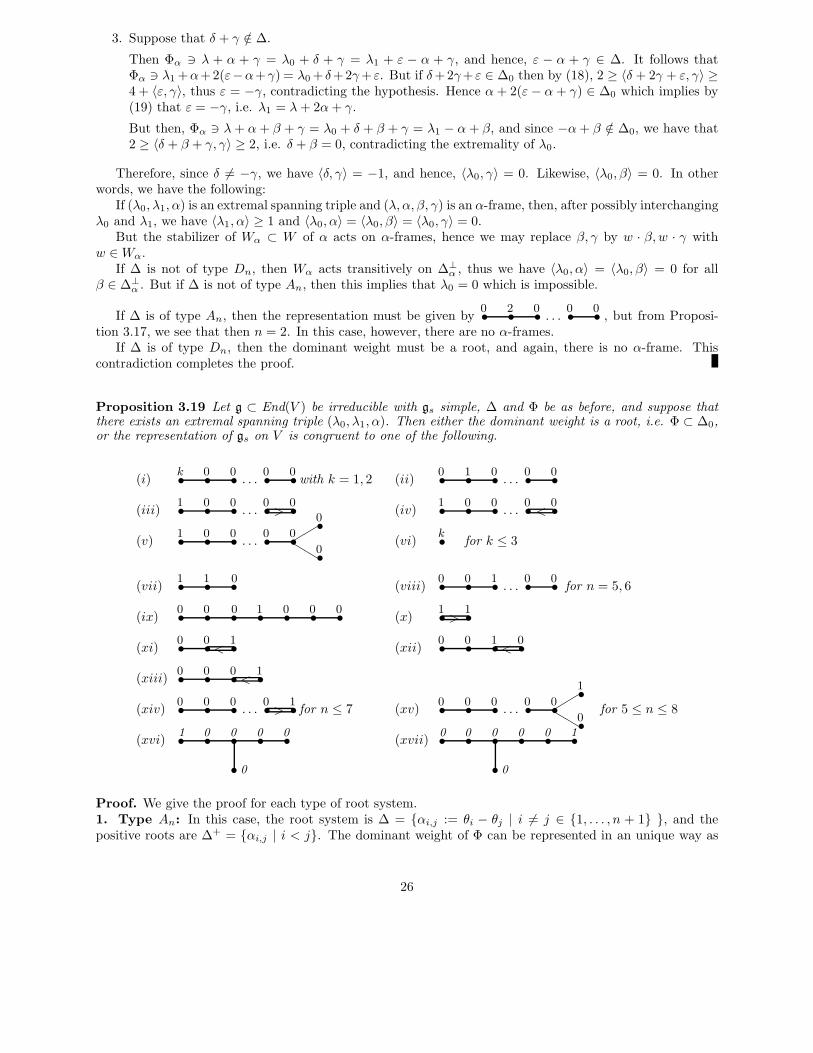
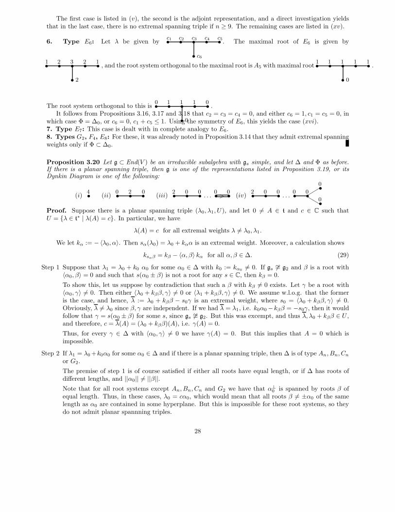
Proposition 3.19 Let g ⊂ End(V ) be irreducible with gs simple, ∆ and Φ be as before, and suppose thatthere exists an extremal spanning triple (λ0, λ1, α). Then either the dominant weight is a root, i.e. Φ ⊂ ∆0,or the representation of gs on V is congruent to one of the following.

(i) . . .s s s s sk 0 0 0 0

with k = 1, 2 (ii) . . .s s s s s0 1 0 0 0

(iii) . . .s s s s> s1 0 0 0 0

(iv) . . .ss s s< s1 0 0 0 0

(v) . . .s s s s s

s

s

1 0 0 0 0

0

0bb

""

(vi) sk

for k ≤ 3

(vii) s s s1 1 0

(viii) . . .s s s s s0 0 1 0 0

for n = 5, 6

(ix) s s s s s s s0 0 0 1 0 0 0

(x) s> s1 1

(xi) s s< s0 0 1

(xii) s s s< s0 0 1 0

(xiii) s s s< s0 0 0 1

(xiv) . . .s s s s> s0 0 0 0 1

for n ≤ 7 (xv) . . .s s s s s

s

s

0 0 0 0 0

1

0bb

""

for 5 ≤ n ≤ 8

(xvi) s s s s s

s

1 0 0 0 0

0

(xvii) s s s s s s

s

0 0 0 0 0 1

0

Proof. We give the proof for each type of root system.1. Type An: In this case, the root system is ∆ = αi,j := θi − θj | i 6= j ∈ 1, . . . , n + 1 , and thepositive roots are ∆+ = αi,j | i < j. The dominant weight of Φ can be represented in an unique way as

26

λ0 = c1θ1 + . . .+ cnθn with integers c1 ≥ . . . ≥ cn ≥ 0. For convenience, we set cn+1 = 0. Note that due tothe symmetry of the root system An we may assume w.l.o.g. that c1 − c2 ≥ cn.

If n = 1 then it is easy to see that there are extremal spanning triples iff the dominant weight is λ0 = kα1,2

with k ≤ 3, and this corresponds to (vi).If rk(gs) ≥ 2, then the only possibile representations (up to congruence) which satisfy the conclusions of

Propositions 3.16, 3.17 and 3.18 are those with the following dominant weights:

λ0 = 2θ1,λ0 = 2θ1 + θ2 + . . .+ θk, k = 2, n− 1, n,λ0 = θ1 + . . .+ θk, 1 ≤ k ≤ n+1

2 .

The Weyl group of An is the permutation group Sn+1 which acts by permutation of the indices ofθ1, . . . , θn+1.

From here, it is now straightforward to investigate each of these representations separately. The resultis that the representations in the second row admit an extremal spanning triple iff k = 2 and n = 3, or ifk = n; the latter correspond to the adjoint representation. In the third row, there are extremal spanningtriples iff k = 4 and n = 7, or k = 3 and n = 5, 6, or k = 1, 2.

This yields precisely the representations (i), (ii), (vii), (viii) and (ix).2. Type Bn: The root system is ∆ = ±θi, ±θi ± θj | i < j, i = 1, . . . , n, and the positive roots are∆+ = θi, θi ± θj | i < j, i = 1, . . . , n. The dominant weight is given by λ0 = c1θ1 + . . . + cnθn withc1 ≥ . . . ≥ cn ≥ 0, where either all ck are integers, or all ck are half-integers.

If all ck are integers, then 0 ∈ Φ, hence, by Proposition 3.14, Φ ⊂ ∆0.Thus, let us assume that the ck are not integers. Then the only representations satisfying the conlusions

of Propositions 3.16 and 3.17 are those whose dominant weights are of the following forms:

λ0 = 32θ1 + 1

2θ2 + . . .+ 12θn,

λ0 = 12θ1 + 1

2θ2 + . . .+ 12θn.

From here, one sees easily that in the first case, there is no extremal spanning triple if n ≥ 3. The casen = 2 is listed in (x). In the second case, one sees that there is no extremal spanning triple if n ≥ 8. Theremaining cases are listed in (xiv).3. Type Cn: The root system is ∆ = ±2θi, ±θi ± θj | i < j, i = 1, . . . , n, and the positive roots are∆+ = 2θi, θi ± θj | i < j, i = 1, . . . , n. The dominant weight is given by λ0 = c1θ1 + . . . + cnθn withintegers c1 ≥ . . . ≥ cn ≥ 0.

The only representations satisfying the conlusions of Propositions 3.16 and 3.17 are those whose dominantweights are of the following forms:

λ0 = 2θ1,λ0 = 2θ1 + θ2 + . . .+ θk, with 2 ≤ k ≤ nλ0 = θ1 + . . .+ θk, with 1 ≤ k ≤ n.

The first case corresponds to the adjoint representation. In the second case, a direct investigation yieldsthat extremal spanning triples exist iff k = n = 2 which is listed in (x). In the third case, one verifies thatthere are extremal spanning triples iff k = n = 4, or k = 3 and n ≤ 4, or if k ≤ 2. If k = 2 then Φ ⊂ ∆0.The remaining cases are listed in (iv), (xi), (xii) and (xiii).4. Type Dn: The root system is ∆ = ±θi ± θj | i < j, i = 1, . . . , n, and the positive roots are∆+ = θi ± θj | i < j, i = 1, . . . , n. The dominant weight is given by λ0 = c1θ1 + . . . + cnθn withc1 ≥ . . . ≥ |cn| ≥ 0, where either all ck are integers, or all ck are half-integers. Using the symmetry of theDynkin diagram, we may assume that cn ≥ 0.

Then the only possibile representations (up to congruence) which satisfy the conclusions of Proposi-tions 3.16, 3.17 and 3.18 are those with the following dominant weights:

λ0 = θ1,λ0 = θ1 + θ2λ0 = 1

2 (θ1 + . . .+ θn).

27

The first case is listed in (v), the second is the adjoint representation, and a direct investigation yieldsthat in the last case, there is no extremal spanning triple if n ≥ 9. The remaining cases are listed in (xv).

6. Type E6: Let λ be given by s s s s s

s

c1 c2 c3 c4 c5

c6

. The maximal root of E6 is given by

s s s s s

s

1 2 3 2 1

2

, and the root system orthogonal to the maximal root isA5 with maximal root s s s s s

s

1 1 1 1 1

0

.

The root system orthogonal to this is s s s s s

s

0 1 1 1 0

0

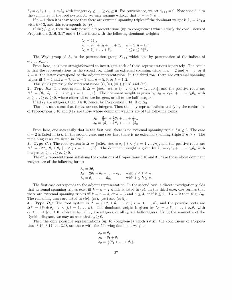
.It follows from Propositions 3.16, 3.17 and 3.18 that c2 = c3 = c4 = 0, and either c6 = 1, c1 = c5 = 0, in

which case Φ = ∆0, or c6 = 0, c1 + c5 ≤ 1. Using the symmetry of E6, this yields the case (xvi).7. Type E7: This case is dealt with in complete analogy to E6.8. Types G2, F4, E8: For these, it was already noted in Proposition 3.14 that they admit extremal spanningweights only if Φ ⊂ ∆0.

Proposition 3.20 Let g ⊂ End(V ) be an irreducible subalgebra with gs simple, and let ∆ and Φ as before.If there is a planar spanning triple, then g is one of the representations listed in Proposition 3.19, or itsDynkin Diagram is one of the following:

(i) s4

(ii) s s s0 2 0

(iii) . . .s s s s> s2 0 0 0 0

(iv) . . .s s s s s

s

s

2 0 0 0 0

0

0bb

""

Proof. Suppose there is a planar spanning triple (λ0, λ1, U), and let 0 6= A ∈ t and c ∈ C such thatU = λ ∈ t∗ | λ(A) = c. In particular, we have

λ(A) = c for all extremal weights λ 6= λ0, λ1.

We let kα := −〈λ0, α〉. Then sα(λ0) = λ0 + kαα is an extremal weight. Moreover, a calculation shows

ksαβ = kβ − 〈α, β〉 kα for all α, β ∈ ∆. (29)

Step 1 Suppose that λ1 = λ0 + k0 α0 for some α0 ∈ ∆ with k0 := kα06= 0. If gs 6∼= g2 and β is a root with

〈α0, β〉 = 0 and such that s(α0 ± β) is not a root for any s ∈ C, then kβ = 0.

To show this, let us suppose by contradiction that such a β with kβ 6= 0 exists. Let γ be a root with〈α0, γ〉 6= 0. Then either 〈λ0 + kββ, γ〉 6= 0 or 〈λ1 + kββ, γ〉 6= 0. We assume w.l.o.g. that the formeris the case, and hence, λ := λ0 + kββ − s0γ is an extremal weight, where s0 = 〈λ0 + kββ, γ〉 6= 0.Obviously, λ 6= λ0 since β, γ are independent. If we had λ = λ1, i.e. k0α0−kββ = −s0γ, then it wouldfollow that γ = s(α0 ± β) for some s, since gs 6∼= g2. But this was excempt, and thus λ, λ0 + kββ ∈ U ,and therefore, c = λ(A) = (λ0 + kββ)(A), i.e. γ(A) = 0.

Thus, for every γ ∈ ∆ with 〈α0, γ〉 6= 0 we have γ(A) = 0. But this implies that A = 0 which isimpossible.

Step 2 If λ1 = λ0 +k0α0 for some α0 ∈ ∆ and if there is a planar spanning triple, then ∆ is of type An, Bn, Cn

or G2.

The premise of step 1 is of course satisfied if either all roots have equal length, or if ∆ has roots ofdifferent lengths, and ||α0|| 6= ||β||.

Note that for all root systems except An, Bn, Cn and G2 we have that α⊥0 is spanned by roots β of

equal length. Thus, in these cases, λ0 = cα0, which would mean that all roots β 6= ±α0 of the samelength as α0 are contained in some hyperplane. But this is impossible for these root systems, so theydo not admit planar spannning triples.

28

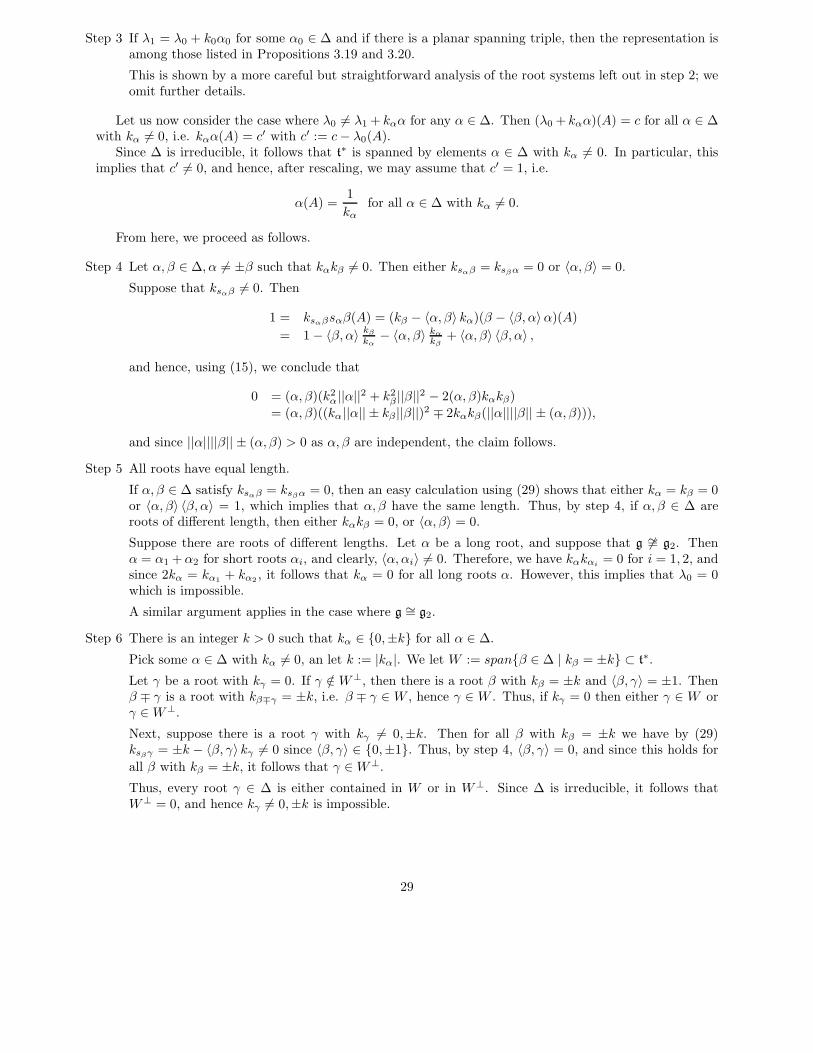
Step 3 If λ1 = λ0 + k0α0 for some α0 ∈ ∆ and if there is a planar spanning triple, then the representation isamong those listed in Propositions 3.19 and 3.20.

This is shown by a more careful but straightforward analysis of the root systems left out in step 2; weomit further details.

Let us now consider the case where λ0 6= λ1 + kαα for any α ∈ ∆. Then (λ0 + kαα)(A) = c for all α ∈ ∆with kα 6= 0, i.e. kαα(A) = c′ with c′ := c− λ0(A).

Since ∆ is irreducible, it follows that t∗ is spanned by elements α ∈ ∆ with kα 6= 0. In particular, thisimplies that c′ 6= 0, and hence, after rescaling, we may assume that c′ = 1, i.e.

α(A) =1

kα

for all α ∈ ∆ with kα 6= 0.

From here, we proceed as follows.

Step 4 Let α, β ∈ ∆, α 6= ±β such that kαkβ 6= 0. Then either ksαβ = ksβα = 0 or 〈α, β〉 = 0.

Suppose that ksαβ 6= 0. Then

1 = ksαβsαβ(A) = (kβ − 〈α, β〉 kα)(β − 〈β, α〉α)(A)

= 1− 〈β, α〉 kβ

kα− 〈α, β〉 kα

kβ+ 〈α, β〉 〈β, α〉 ,

and hence, using (15), we conclude that

0 = (α, β)(k2α||α||

2 + k2β ||β||

2 − 2(α, β)kαkβ)

= (α, β)((kα||α|| ± kβ ||β||)2 ∓ 2kαkβ(||α||||β|| ± (α, β))),

and since ||α||||β|| ± (α, β) > 0 as α, β are independent, the claim follows.

Step 5 All roots have equal length.

If α, β ∈ ∆ satisfy ksαβ = ksβα = 0, then an easy calculation using (29) shows that either kα = kβ = 0or 〈α, β〉 〈β, α〉 = 1, which implies that α, β have the same length. Thus, by step 4, if α, β ∈ ∆ areroots of different length, then either kαkβ = 0, or 〈α, β〉 = 0.

Suppose there are roots of different lengths. Let α be a long root, and suppose that g 6∼= g2. Thenα = α1 +α2 for short roots αi, and clearly, 〈α, αi〉 6= 0. Therefore, we have kαkαi

= 0 for i = 1, 2, andsince 2kα = kα1

+ kα2, it follows that kα = 0 for all long roots α. However, this implies that λ0 = 0

which is impossible.

A similar argument applies in the case where g ∼= g2.

Step 6 There is an integer k > 0 such that kα ∈ 0,±k for all α ∈ ∆.

Pick some α ∈ ∆ with kα 6= 0, an let k := |kα|. We let W := spanβ ∈ ∆ | kβ = ±k ⊂ t∗.

Let γ be a root with kγ = 0. If γ /∈ W⊥, then there is a root β with kβ = ±k and 〈β, γ〉 = ±1. Thenβ ∓ γ is a root with kβ∓γ = ±k, i.e. β ∓ γ ∈ W , hence γ ∈ W . Thus, if kγ = 0 then either γ ∈ W orγ ∈ W⊥.

Next, suppose there is a root γ with kγ 6= 0,±k. Then for all β with kβ = ±k we have by (29)ksβγ = ±k − 〈β, γ〉 kγ 6= 0 since 〈β, γ〉 ∈ 0,±1. Thus, by step 4, 〈β, γ〉 = 0, and since this holds for

all β with kβ = ±k, it follows that γ ∈W⊥.

Thus, every root γ ∈ ∆ is either contained in W or in W⊥. Since ∆ is irreducible, it follows thatW⊥ = 0, and hence kγ 6= 0,±k is impossible.

29

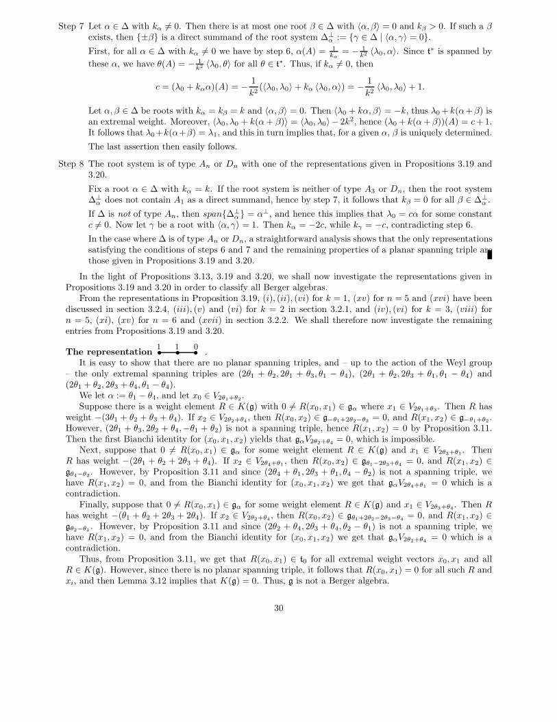
Step 7 Let α ∈ ∆ with kα 6= 0. Then there is at most one root β ∈ ∆ with 〈α, β〉 = 0 and kβ > 0. If such a βexists, then ±β is a direct summand of the root system ∆⊥

α := γ ∈ ∆ | 〈α, γ〉 = 0.

First, for all α ∈ ∆ with kα 6= 0 we have by step 6, α(A) = 1kα

= − 1k2 〈λ0, α〉. Since t∗ is spanned by

these α, we have θ(A) = − 1k2 〈λ0, θ〉 for all θ ∈ t∗. Thus, if kα 6= 0, then

c = (λ0 + kαα)(A) = −1

k2(〈λ0, λ0〉+ kα 〈λ0, α〉) = −

1

k2〈λ0, λ0〉+ 1.

Let α, β ∈ ∆ be roots with kα = kβ = k and 〈α, β〉 = 0. Then 〈λ0 + kα, β〉 = −k, thus λ0 +k(α+β) isan extremal weight. Moreover, 〈λ0, λ0 + k(α+ β)〉 = 〈λ0, λ0〉 − 2k2, hence (λ0 + k(α+ β))(A) = c+ 1.It follows that λ0+k(α+β) = λ1, and this in turn implies that, for a given α, β is uniquely determined.

The last assertion then easily follows.

Step 8 The root system is of type An or Dn with one of the representations given in Propositions 3.19 and3.20.

Fix a root α ∈ ∆ with kα = k. If the root system is neither of type A3 or Dn, then the root system∆⊥

α does not contain A1 as a direct summand, hence by step 7, it follows that kβ = 0 for all β ∈ ∆⊥α .

If ∆ is not of type An, then span∆⊥α = α⊥, and hence this implies that λ0 = cα for some constant

c 6= 0. Now let γ be a root with 〈α, γ〉 = 1. Then kα = −2c, while kγ = −c, contradicting step 6.

In the case where ∆ is of type An or Dn, a straightforward analysis shows that the only representationssatisfying the conditions of steps 6 and 7 and the remaining properties of a planar spanning triple arethose given in Propositions 3.19 and 3.20.

In the light of Propositions 3.13, 3.19 and 3.20, we shall now investigate the representations given inPropositions 3.19 and 3.20 in order to classify all Berger algebras.

From the representations in Proposition 3.19, (i), (ii), (vi) for k = 1, (xv) for n = 5 and (xvi) have beendiscussed in section 3.2.4, (iii), (v) and (vi) for k = 2 in section 3.2.1, and (iv), (vi) for k = 3, (viii) forn = 5, (xi), (xv) for n = 6 and (xvii) in section 3.2.2. We shall therefore now investigate the remainingentries from Propositions 3.19 and 3.20.

The representation s s s1 1 0

.It is easy to show that there are no planar spanning triples, and – up to the action of the Weyl group

– the only extremal spanning triples are (2θ1 + θ2, 2θ1 + θ3, θ1 − θ4), (2θ1 + θ2, 2θ3 + θ1, θ1 − θ4) and(2θ1 + θ2, 2θ3 + θ4, θ1 − θ4).

We let α := θ1 − θ4, and let x0 ∈ V2θ1+θ2.

Suppose there is a weight element R ∈ K(g) with 0 6= R(x0, x1) ∈ gα where x1 ∈ V2θ1+θ3. Then R has

weight −(3θ1 + θ2 + θ3 + θ4). If x2 ∈ V2θ2+θ4, then R(x0, x2) ∈ g−θ1+2θ2−θ3

= 0, and R(x1, x2) ∈ g−θ1+θ2.

However, (2θ1 + θ3, 2θ2 + θ4,−θ1 + θ2) is not a spanning triple, hence R(x1, x2) = 0 by Proposition 3.11.Then the first Bianchi identity for (x0, x1, x2) yields that gαV2θ2+θ4

= 0, which is impossible.Next, suppose that 0 6= R(x0, x1) ∈ gα for some weight element R ∈ K(g) and x1 ∈ V2θ3+θ1

. ThenR has weight −(2θ1 + θ2 + 2θ3 + θ4). If x2 ∈ V2θ4+θ1

, then R(x0, x2) ∈ gθ1−2θ3+θ4= 0, and R(x1, x2) ∈

gθ4−θ2. However, by Proposition 3.11 and since (2θ4 + θ1, 2θ3 + θ1, θ4 − θ2) is not a spanning triple, we

have R(x1, x2) = 0, and from the Bianchi identity for (x0, x1, x2) we get that gαV2θ4+θ1= 0 which is a

contradiction.Finally, suppose that 0 6= R(x0, x1) ∈ gα for some weight element R ∈ K(g) and x1 ∈ V2θ3+θ4

. Then Rhas weight −(θ1 + θ2 + 2θ3 + 2θ4). If x2 ∈ V2θ2+θ4

, then R(x0, x2) ∈ gθ1+2θ2−2θ3−θ4= 0, and R(x1, x2) ∈

gθ2−θ1. However, by Proposition 3.11 and since (2θ2 + θ4, 2θ3 + θ4, θ2 − θ1) is not a spanning triple, we

have R(x1, x2) = 0, and from the Bianchi identity for (x0, x1, x2) we get that gαV2θ2+θ4= 0 which is a

contradiction.Thus, from Proposition 3.11, we get that R(x0, x1) ∈ t0 for all extremal weight vectors x0, x1 and all

R ∈ K(g). However, since there is no planar spanning triple, it follows that R(x0, x1) = 0 for all such R andxi, and then Lemma 3.12 implies that K(g) = 0. Thus, g is not a Berger algebra.

30

The representation s s s s s s0 0 1 0 0 0

.This is the representation of gl(7,C) on W := Λ3V with V = C7. Every weight is extremal, and – up

to the action of the Weyl group – the only spanning triples are (θ1 + θ2 + θ3, θ4 + θ5 + θ6, θ1 − θ7) and(θ1 + θ2 + θ3, θ1 + θ4 + θ5, θ1− θ7). Thus, by Proposition 3.11, the only possible weights ρ of K(g) are ρ = θi,some i.

Suppose there is an R ∈ K(g) of weight ρ = θ1. We let e1, . . . , e7 be the standard basis of V andwrite eijk := ei ∧ ej ∧ ek, which spans the weight space Wθi+θj+θk

. Then, for weight reasons, we haveR(e123, e456) ∈ gθ1−θ7

, and hence, there is some c ∈ C with R(e123, e456)y = c(e123 ∧ e456 ∧ y)e1, where weidentify Λ7V and C.

Now gR = R for all g ∈ SL(7,C) with ge1 = e1. Using this equivariance, we conclude that R(e1 ∧α2, α3)y = c(e1 ∧ α2 ∧ α3 ∧ y)e1 for all αi ∈ ΛiV .

But now, applying the first Bianchi identity to (e123, e456, e457) and using that for weight reasonsR(e456, e457) = 0, we get that 2ce145 = 0, i.e. c = 0, which means that R(e1 ∧ α2, ) = 0 for all α2 ∈ Λ2V .Then, from the Bianchi identity, it follows that R(α, β)(e1 ∧ α2) = 0 for all α, β ∈ W and α2 ∈ Λ2V . Butthis implies that R(α, β)y = cy + τ(y)e1 for all y ∈ V , where c ∈ C and τ ∈ V ∗ with τ(e1) = −3c.

For weight reasons, R(e234, e567) ∈ t0 and therefore, R(e234, e567)y = c((e1 ∧ e234 ∧ e567)y − 3(y ∧ e234 ∧e567)e1) for some c ∈ C. Using that gR = R for all g ∈ SL(7,C) with ge1 = e1, we conclude thatR(α, β)y = c((e1 ∧ α ∧ β)y − 3(y ∧ α ∧ β)e1) for all α, β ∈ W and some c ∈ C.

But now, it is easy to show that this map R satisfies the Bianchi identity only if c = 0, i.e. R = 0 whichis impossible. From here, we get that K(g) = 0, hence g is not Berger.

The representation s s s s s s s0 0 0 1 0 0 0

.This is the representation of gl(8,C) on W := Λ4V with V = C8. It is easy to see that – up to the action

of the Weyl group – the only spanning triple is (θ1 + θ2 + θ3 + θ4, θ1 + θ5 + θ6 + θ7, θ1 − θ8). Since thereare no planar spanning triples, it follows by Proposition 3.11 that the only possible weight of K(g) is ρ = 0,i.e. K(g) is a trivial g-module. Thus, dim(K(g)) ≤ 1 by Proposition 3.9, and in fact, one can show thatdim(K(g)) = 1 and it is spanned by the curvature map of the symmetric space EC

7 /SL(8,C).

The representation s> s1 1

.It is easy to see that – up to the action of the Weyl group – the only extremal spanning triples are

(2θ1 + θ2,−θ1 − 2θ2, 2θ1), (θ1 + 2θ2, θ1 − 2θ2, 2θ1), (2θ1 − θ2, θ1 + 2θ2, 2θ1), (2θ1 + θ2, 2θ1 − θ2, 2θ1), and(2θ1 − θ2,−θ1 + 2θ2, θ1 + θ2).

Let x ∈ V2θ1+θ2, y ∈ V−θ1−2θ2

and z ∈ V−2θ1−θ2. Suppose that there is a weight element R ∈ K(g)

with 0 6= R(x, y) ∈ g2θ1. Then R has weight −θ1 − θ2, thus R(x, z) ∈ g−θ1−θ2

and R(y, z) ∈ g−4θ1−2θ2= 0.

However, since (2θ1+θ2,−θ1−2θ2,−θ1−θ2) is not a spanning triple, we haveR(x, z) = 0 by Proposition 3.11.Thus, from the Bianchi identity we get that g2θ1

V−2θ1−θ2= 0 which is impossible. Likewise, we exclude that

R(V2θ1−θ2, Vθ1+2θ2

) 6= 0 and R(V2θ1+θ2, V2θ1−θ2

) 6= 0 for weight elements R ∈ K(g).Thus, if R ∈ K(g) is a weight element of weight ρ 6= 0, then R(x, y) ∈ t0 for all extremal weight vectors

x, y ∈ V . But g ⊂ csp(V,Ω), and hence we must have R(x, y) ∈ t for all such x, y ∈ V . Hence, if R(x, y) 6= 0for extremal weight vectors of weights λ0 and λ1, then there must be a planar spanning triple (λ0, λ1, U)with U being a linear hyperplane and λ0 + λ1 = ρ 6= 0. However, it is easy to see that this is impossible.

It follows that, if R ∈ K(g) is a weight element of weight ρ 6= 0, then R(x, y) = 0 for all extremal weightvectors x, y ∈ V , and from here one can conlude that R = 0 which is impossible, and therefore, ρ = 0 isthe only weight, i.e. K(g) is a trivial g-module. But g ⊂ csp(V ) and therefore, Proposition 3.9 implies thatK(g) = 0 and hence, g is not Berger.

The representation s s s< s0 0 1 0

.The only extremal spanning triples are – up to the action of the Weyl group – (θ1 + θ3 + θ4, θ2 − θ3 −

θ4, θ1+θ2) and (θ1+θ2+θ3, θ1−θ2−θ3, 2θ1). Since there are no extremal spanning triples, there is no weightelement R ∈ K(g) with R(x, y) ⊂ t0 for all x, y ∈ V , hence by Proposition 3.11, the only possible weight is

31

ρ = 0, i.e. K(g) is a trivial g-module. But again, g ⊂ csp(V ), and hence K(g) = 0 by Proposition 3.9, i.e. g

is not Berger.

The representation s s s< s0 0 0 1

.The only extremal spanning triples are, up to the action of the Weyl group, (θ1 + θ2 + θ3 + θ4, θ1 −

θ2 − θ3 − θ4, 2θ1). Since there are no extremal spanning triples, there is no weight element R ∈ K(g) withR(x, y) ⊂ t0 for all x, y ∈ V , hence by Proposition 3.11, the only possible weight is ρ = 0, i.e. K(g) is a trivialg-module and hence, by Proposition 3.9, it follows that dimK(g) ≤ 1. But indeed, K(g) is one-dimensionaland spanned by the curvature map of the symmetric space EC

6 /Sp(4,C).

The representation . . .s s s s s

s

s

0 0 0 0 0

1

0bb

""

for n = 7.

This representation is the complex spinor representation ∆+14. A calculation shows that Λ2∆+

14∼= Λ5V ⊕V

where V = C14.Every weight is extremal, and one calculates that the only spanning triples are, up to the action of the

Weyl group, (12 (θ1 + . . .+ θ7),

12 (θ1 + θ2 + θ3 − θ4− . . .− θ7), θ1 + θ2) and (1

2 (θ1 + . . .+ θ7),12 (θ1 − θ2− . . .−

θ7), θ1 +θ2). Thus, for any R ∈ K(g), we have R(x, y) = 0 if x, y are weight vectors of weights 12 (θ1 + . . .+θ7)

and 12 (θ1 + . . . + θ5 − θ6 − θ7), respectively, i.e. if x ∧ y is the dominant weight vector of Λ5V ⊂ Λ2∆+

14.Therefore, K(g) ⊂ V ⊗ g.

But now, we let x, y, z be weight vectors of weights 12 (θ1 + . . .+θ7),

12 (θ1−θ2− . . .−θ7) and 1

2 (−θ1−θ2 +

θ3 . . .+ θ7), respectively. Then x ∧ z, y ∧ z ∈ Λ5V ⊂ Λ2∆+14, and hence R(x, z) = R(y, z) = 0. Thus, by the

Bianchi identity, R(x, y)z = 0 for all R ∈ K(g). However, if K(g) 6= 0 then there must be some R ∈ K(g)with 0 6= R(x, y) ∈ gθ1+θ2

by Proposition 3.11 which is a contradiction. Thus, K(g) = 0, and g is not Berger.

The representation . . .s s s s s

s

s

0 0 0 0 0

1

0bb

""

for n = 8.

This representation is the complex spinor representation ∆+16. Note that there is a g-invariant inner

product, i.e. g ⊂ co(∆+16). Moreover, every weight is extremal.

The only spanning triples are, up to the action of the Weyl group, (12 (θ1 + . . .+ θ8),

12 (θ1 + θ2− θ3− . . .−

θ8), θ1 + θ2). Thus, if R ∈ K(g) was a weight vector of weight ρ 6= 0, then this implies that R(x, y) ∈ t0 forall x, y ∈ V . But since there are no planar spanning triples, it follows that R = 0 which is impossible.

Therefore, ρ = 0 is the only weight ofK(g), i.e. K(g) is trivial, and then by Proposition 3.9, dimK(g) ≤ 1.In fact, dimK(g) = 1, and is spanned by the curvature tensor of the symmetric space EC

8 /Spin(16,C).

The representations . . .s s s s> s0 0 0 0 1

for n ≤ 7.

These are the complex spinor representations of spin(2n+ 1) on ∆2n+1∼= ∆+

2n+2. Since spin(2n+ 1) ⊂spin(2n + 2), it follows that K(spin(2n + 1)) ⊂ K(spin(2n + 2)), and hence by the above we see thatK(spin(2n+ 1)) = 0 for n = 6, 7.

For n = 5, we consider K(h) ⊂ K(spin(12)) where h = spin(11) acts on V = ∆11∼= ∆+

12. By Proposi-tion 3.8, each R ∈ K(h) must be of the form R(x, y) = Ω(x, y)h+ x (hy)− y (hx) for some h ∈ spin(12).

Let v ∈ h⊥. Then 0 = (R(x, y), v) = Ω(x, y)B(h, v) + Ω(vx, hy) − Ω(vy, hx) =Ω(x, y)B(h, v) − Ω((hv + vh)x, y) for all x, y ∈ ∆11 and hence,

hv + vh = B(h, v)IdV

for all h ∈ K(h) and v ∈ h⊥.However, a calculation then shows that this implies that h = 0, i.e. K(h) = 0 and h is not Berger.For n = 4, we consider h = spin(9) acting on V = ∆9. It is well known that h ⊂ so(V ), and hence

h ⊕ CIdV is not Berger by Proposition 3.2. Also, a calculation shows that K(h) is one-dimensional and isspanned by the curvature of the symmetric space FC

4 /(Spin(9,C)).

32

For n = 3, we have h = spin(7) acting on V = ∆7. Again, h ⊂ so(V ), hence h ⊕ CIdV is not Berger.On the other hand, spin(7) is one of the classically known examples of Riemannian holonomies, hence it isBerger.

The representations s4, s s s0 2 0

, . . .s s s s> s2 0 0 0 0

, . . .s s s s s

s

s

2 0 0 0 0

0

0bb

""

.

For these representation, there are no extremal spanning triples. Also, one sees that the only planarspanning triples are of the form (λ0,−λ0, U). Thus, if R ∈ K(g) is a weight element of weight ρ 6= 0, thenR(x, y) = 0 for all extremal weight vectors x, y ∈ V . However, it is not hard to see that this implies R = 0which is impossible.

Therefore, for all these representations, ρ = 0 is the only weight of K(h), i.e. K(h) is a trivial h-module,and Proposition 3.9 implies that dim(K(h)) ≤ 1. In fact, one calculates that dimK(h) = 1, being spannedby the curvature of the symmetric spaces SL(n,C)/SO(n,C) for n ≥ 3, n 6= 4.The adjoint representations

Let g be a complex simple Lie algebra with rk(g) ≥ 2, acting on V = g via the adjoint representationad : g → End(g). Then ad(g) ⊂ so(g) with the inner product being given by the Killing form on g, andhence by Proposition 3.2, ad(g)⊕CIdg is not Berger. Fix elements 0 6= Aα ∈ gα for each α ∈ ∆. Moreover,we denote elements of t by A0, B0, . . ..

Suppose there is an element R ∈ K(ad(g)) of weight ρ ∈ ∆. We denote R(x, y) by x, y, and thus, thefirst Bianchi identity reads

[x, y, z] + [y, z, x] + [z, x, y] = 0. (30)

Moreover, since R is symmetric, we have the identity

B(x, y, [z, w]) = B(z, w, [x, y]). (31)

In particular, x, y = 0 whenever [x, y] = 0, thus A0, B0 = 0 for all A0, B0 ∈ t.Let −ρ 6= α ∈ ∆ be a root such that α + ρ ∈ ∆. Then, for weight reasons, there is a σα ∈ t∗ such

that A0, Aα = σα(A0)Aα+ρ for all A0 ∈ t. Now applying (30) to (x, y, z) = (A0, Aα, A−(α+ρ)) impliesthat σα(A0)[Aα+ρ, A−(α+ρ)] + σ−(α+ρ)(A0)[Aα, A−α] = 0. Since α, α + ρ are linearly independent, so are[Aα, A−α] and [Aρ+α, A−(ρ+α)], and thus σα = 0 for all α 6= −ρ, i.e.

A0, Aα = 0 for all α ∈ ∆, α 6= −ρ.

If α, β 6= −ρ are roots such that α + β + ρ 6= 0, then applying (30) to (x, y, z) = (A0, Aα, Aβ), we concludethat Aα, Aβ = 0 for all such roots.

If α, β, γ ∈ ∆ are pairwise different roots such that α + β + ρ = 0, then applying (30) to (x, y, z) =(Aα, Aβ , Aγ) and using the preceding remark, we get γ(Aα, Aβ) = 0 for all such roots γ. All this nowimplies that

Aα, Aβ = 0 for all roots α, β 6= −ρ.

But then, if x, y ∈ g are arbitrary, applying (31) with z = A0, w = Aα, we get that B(x, y, Aα) = 0for all α 6= −ρ; choosing α, β ∈ ∆ with α + β + ρ = 0 and applying (31) with z = Aα, w = Aβ , we getB(x, y, A−ρ) = 0. Finally, for z = Aα, w = A−α, we get B(x, y, [Aα, A−α]) = 0 for all α 6= ±ρ. All ofthis implies that x, y = 0 for all x, y ∈ g, i.e. R = 0 which is impossible.

This implies that K(ad(g)) does not have roots as weights, and hence is a trivial g-module. From here,Proposition 3.9 implies that dimK(ad(g)) ≤ 1, and clearly, dimK(ad(g)) = 1, spanned by x, y = [x, y].This is the curvature of the symmetric space (G×G)/∆G.The representations whose dominant weight is a short root

A similar argument as for the adjoint representations applies to these representations, as long as dim V0 ≥2, where V0 denotes the 0-weight space, and shows that all those are symmetric. This implies in particular,that the corresponding subgroups are symmetric if ∆ is of type Cn with n ≥ 3, or if ∆ is of type F4. Thecorresponding symmetric spaces are SL(2n,C)/Sp(n,C) for n ≥ 3, and EC

6 /FC

4 .

33

If ∆ is of type Bn, then we obtain the standard representation of so(2n+1) which was already discussed.If ∆ is of type G2, we get the 7-dimensional representation of G2; this representation is orthogonal, thus itsconformal extension is not Berger by Proposition 3.2. The representation of G2 itself, however, is one of theclassically known examples of a Berger group [Bes].

3.5 Complex tensor representations

In this section, we shall classify the Berger algebras whose semi-simple part is not simple. In the complexcategory, this implies that the representation is a tensor representation. That is, we have V = V1 ⊗ V2.Moreover, there is a natural map End(V1)⊕End(V2)→ End(V ) which is induced by the tensor representation.We denote the image of this map by g ⊂ End(V ) and its semi-simple part by g0.

It is not hard to see that any irreducible Lie algebra h ⊂ g is of the form h = h1 ⊕ h2 with irreduciblehi ⊂ End(Vi). We denote the sets of weights and roots of hi by Φi and ∆i, respectively. Then ∆ = ∆1 ∪∆2

and Φ = Φ1 + Φ2. Also, if α ∈ ∆1, then Φα = Φ1α + Φ2.

We first consider the case where dimVi ≥ 3 for i = 1, 2. We get the following classification.

Proposition 3.21 Let V1, V2 be finite dimensional complex vector spaces with ni := dimVi ≥ 3, and letV = V1 ⊗ V2, g, g0 ⊂ End(V ) as above.

If h ⊂ g acts irreducibly on V , then h is a Berger algebra iff it is congruent to an entry of the followinglist where in each case, V = Cn1 ⊗ Cn2 .

h K(h) symmetric

gl(n1,C)⊕ gl(n2,C) V ∗ ⊗ V ∗ no

sl(n1,C)⊕ sl(n2,C) ⊙2V ∗ no

so(n1,C)⊕ so(n2,C) C yes

sp(

n1

2 ,C)

⊕ sp(

n2

2 ,C)

C yes

For the proof, we need several Lemmas.

Lemma 3.22 Let V = V1 ⊗ V2, g, g0 ⊂ End(V ) as above, and suppose that h ∼= h1 ⊕ h2 ⊂ g is a Bergeralgebra. Then Φi

α consists of at most two elements for every α ∈ ∆i.

Proof. Suppose there is an α ∈ ∆1 for which Φ1α has more than two elements. By Proposition 3.11, there

is a spanning triple (λ0 + µ0, λ1 + µ1, α), λi ∈ Φ1, µi ∈ Φ2. Since dimV2 ≥ 3, Φ2 contains at least threeelements. Thus, there are elements λ ∈ Φ1

α, λ 6= λ0, λ1 and µ ∈ Φ2, µ 6= µ1, µ2. But then, λ+ µ ∈ Φα, and

(λ− λi) + (µ− µi) /∈ ∆. This contradiction finishes the proof.

Lemma 3.23 Let h ⊂ End(V ) be an irreducible subalgebra, and let hs be the semi-simple part of h. Supposethat for some α ∈ ∆ the set Φα contains at most two elements. Then hs is conjugate to one of the followingrepresentations.

1. sl(n,C) acting on Cn; in this case, Φα is singleton for all α ∈ ∆.

2. so(n,C) acting on Cn. In this case, Φα contains two elements for all α ∈ ∆, and their sum equals α.

3. sp(n,C) acting on C2n. In this case, Φα contains two elements if α ∈ ∆ is short, and their sum equalsα, and Φα = 1

2α if α ∈ ∆ is long.

4. g2 acting on C7. Then Φα contains two elements if α is long, but three elements if α is short.

34

5. spin(7,C) acting on C8. Then Φα contains two elements if α is long, and their sum equals α, and Φα

contains three elements if α is short.

6. sl(2,C) ⊕ sl(n,C) acting on C2 ⊗ Cn; in this case, Φα contains two elements if α is a root of thesl(n,C)-summand, and contains n elements if α is a root of the sl(2,C)-summand.

7. sl(2,C) ⊕ sp(n,C) acting on C2 ⊗ C

2n; in this case, Φα contains two elements if α is a long root ofthe sp(n,C)-summand; Φα contains four elements if α is a short root of the sp(n,C)-summand, and itcontains 2n elements if α is a root of the sl(2,C)-summand.

Proof. Suppose that Φα contains at most two elements for some α ∈ ∆. Clearly, | 〈λ, α〉 | ≤ 2 for all λ ∈ Φ,since otherwise λ+ kα ∈ Φα for k = 1, 2, 3.

Suppose that 〈λ, α〉 = −2 for some λ ∈ Φ. Then Φα = λ+α, λ+2α. If there is a β ∈ ∆ with 〈β, α〉 = 1then, after replacing β by α−β if necessary, we may assume that 〈λ, β〉 < 0, and thus λ+α+β ∈ Φα, whichis a contradiction, as β 6= 0, α. Thus, there is no β ∈ ∆ with 〈β, α〉 = 1. This means that either rk hs = 1,or ∆ is of type Bn with α short. In the first case hs ⊂ End(V ) is the standard representation of so(3,C) onC3, while in the second case we have the standard representation of so(2n+ 1,C) on C2n+1, n ≥ 2.

Next, suppose that | 〈λ, α〉 | ≤ 1 for all λ ∈ Φ, and suppose there is a β ∈ ∆⊥α with 〈λ, β〉 = −1. Then

Φα = λ + α, λ + α + β. Thus, β ∈ ∆⊥α with this property is unique, and it follows that ±β is a direct

summand of ∆⊥α .

This implies that ∆ is of type A3, Bn (with α long), Cn (with α short), Dn, G2 or ∆ contains A1 as adirect summand. For all these, one can show that they yield the representations listed above.

Finally, suppose that 〈λ, α〉 = 1 and 〈λ, β〉 = 0 for all β ∈ ∆⊥α . If ∆ is not of type An, then this implies

that λ = 12α which is possible only if ∆ is of type Cn, and this yields the standard representation of sp(n,C).

If ∆ is of type An, then all this implies that the representation is the standard representation of sl(n,C) on

Cn.

Proof of Proposition 3.21. Since by Lemma 3.22 Φiα must contain at most two elements for all α ∈ ∆i,

it follows from Lemma 3.23 that only cases 1,2,3 and case 6 for n = 2 can occur. In the latter case, we havehs∼= sl(2,C)⊕ sl(2,C) acting on C2 ⊗ C2, which is equivalent to the standard representation of so(4,C) on

C4.Thus, if h = h1 ⊕ h2 ⊂ g is a Berger algebra, then the semi-simple parts (hi)s are either sl(ni,C),

so(ni,C) or sp(ni

2 ,C) with their standard representations. But now from the explicit description of thecurvature tensor in (24), it follows that h1 = so(n1,C) implies h2 = so(n2,C) and dimK(h) = 1, and

likewise, h1 = sp(n1

2 ,C) implies h2 = sp(n2

2 ,C) and dimK(h) = 1. This proves the proposition.

Now we turn to the case where V = V1 ⊗ V2 with dimV1 = 2. In this case, h ∼= sl(2,C) ⊕ h2 with anirreducible subalgebra h2 ⊂ End(V2). We begin with the following proposition.

Proposition 3.24 Let V = V1 ⊗V2 and h, h2 as in the preceding paragraph, and suppose that h is a Bergeralgebra. If sl(2,C) acts trivially on K(h) then h is symmetric.

Proof. We fix a basis e1, e2 of V1, and let 〈 , 〉 denote the determinant of V1. Elements of V1 and V2 will bedenoted by e, f, . . . and x, y, . . . respectively.

Since K1(h) ⊂ V ∗ ⊗K(h) ∼= V ∗1 ⊗ (V ∗

2 ⊗K(h)) and since, by hypothesis, V ∗2 ⊗K(h) is a trivial sl(2,C)-

module, it follows that K1(h) = V ∗1 ⊗W for some subspace W ⊂ V ∗

2 ⊗K(h). Pick φ1 ∈ W , and define anelement φ ∈ K1(h) by

φ(e1 ⊗ x) := 0, φ(e2 ⊗ x) := φ1(x).

Then the second Bianchi identity for the triple (e1 ⊗ x, e1 ⊗ y, e2 ⊗ z) yields φ1(z)(e1 ⊗ x, e1 ⊗ y) = 0, andhence, by polarization, φ1(z)(e⊗ x, f ⊗ y) = 〈e, f〉ψ(z)(x, y), where ψ(z) ∈ ⊙2V ∗

2 ⊗ h. Since φ1(z) ∈ W issl(2,C)-invariant, so is ψ(z), and hence ψ(z) ∈ ⊙2V ∗

2 ⊗ h2.

35

Next, consider the first Bianchi identity for φ1(z) ∈ K(h) for the triple (e1⊗ x, e1⊗ y, e2⊗w). It follows

that ψ(z)(w, x) · y = ψ(z)(w, y) · x, and hence, ψ(z) ∈ h(2)2 .

But there are only four irreducible Lie algebras h2 for which h(2)2 6= 0 (cf. Table 4), and for these it is

easy to show that K(h) is not a trivial sl(2,C)-module. Thus, we have that ψ = 0, i.e. W = 0, and hence,

K1(h) = 0.

Now we obtain the following classification.

Proposition 3.25 Let V = V1 ⊗ V2 and h, h2 as above, i.e. dimV1 = 2 and h2 ⊂ End(V2) is irreducible,and suppose that h = sl(2,C) ⊕ h2 ⊂ End(V ) is a non-symmetric Berger algebra. Then h2 is congruent tothe standard representation of one of the Lie algebras so(n,C), sp(n,C), sl(n,C) or gl(n,C).

We begin with the following Lemma.

Lemma 3.26 Let V = V1⊗V2 and h, h2 as above. If h is a non-symmetric Berger algebra then Φ2α contains

at most two elements for some α ∈ ∆2. Moreover, if the semi-simple part of h2 is simple, then this holdstrue for all α ∈ ∆2.

Proof. The claim is obvious if dimV2 = 2. Thus, we assume from now on the dimV2 ≥ 3.Let W ⊂ K(h) be the subspace spanned by weight elements R ∈ K(h) of weight −2ψ0 + µ, where µ

is in the weight lattice of h2 and ψ0 is the generator of the weight lattice of sl(2,C). Since h is a non-symmetric Berger algebra, Proposition 3.24 implies that W 6= 0. Evidently, W is h2-invariant. Thus,s := R(u, v) | u, v ∈ V,R ∈W ⊂ h is also h2-invariant.

Suppose s ⊂ h1. Then the first Bianchi identity for (e1 ⊗ x, e1 ⊗ y, e2 ⊗ z) for independent x, y, z ∈ V2

yields R = 0, i.e. W = 0 which is a contradiction.Thus, 0 6= s ∩ h2 ⊳ h2. If α is a root of s ∩ h2, then evidently, there is a weight element R ∈ W of

weight −2ψ0 + µ, and weight vectors u, v ∈ V such that R(u, v) = Aα. Then u, v have weights ψ0 + λi,i = 0, 1, for some λi ∈ Φ2, and by Proposition 3.11, (ψ0 + λ0, ψ0 + λ1, α) is a spanning triple. Note thatΦα = ±ψ0 + λ | λ ∈ Φ2

α.If there was an element λ ∈ Φ2

α with λ 6= λ0, λ1, then −ψ0 + λ ∈ Φ2α, but (−ψ0 + λ) − (ψ0 + λi) /∈ ∆,

which is a contradiction. Therefore, Φ2α contains at most the two elements λ0 and λ1.

Finally, if h2 is simple, then s ∩ h2 = h2, and hence the above argument applies to all α ∈ ∆2.

Proof of Proposition 3.25. By Lemmas 3.23 and 3.26, we only must rule out the representation withh2 = sl(2,C) ⊕ h3 on C2 ⊗ Cn, where h3 = sl(n,C) or sp(n

2 ,C) with their standard representations. Inthese cases, h ∼= so(4,C)⊕ h3 acting on V = C4 ⊗Cn. However, these were already shown not to be Berger

algebras in Proposition 3.21.

4 Existence results

In the previous chapter, we have characterized those irreducible subalgebras h ⊂ End(V ) which are Bergerand hence satisfy a necessary condition to occur as the holonomy of a torsion free connection on somemanifold. However, this is still far from showing the existence of such connections. In fact, even in the caseof Riemannian holonomies, more than three decades passed between the classification of Riemannian Bergeralgebras [Ber1] and the proof of their existence in all cases [Br2].

The method that was used in the latter reference is based on the method of Exterior Differential Systemsand will be described in the following section. It turns out that this method applies to most other cases ofBerger algebras as well, thus showing the existence of torsion free connections with these holonomies. Weshall give only a brief outline of this method in section 4.1, but shall refer the reader to [Br2, Br3, Br4] fora more thorough treatement.

36

There is another method to construct torsion free connections with prescribed holonomy which is basedon deformations of linear Poisson structures [CMS1, CMS2]. As it turns out, this method is universal in theclass of symplectic holonomies, that is, any torsion free connection whose irreducible holonomy group H isproperly contained in Sp(V,Ω) locally comes from this construction. We shall summarize this method andsome of its applications in section 4.3.

4.1 Exterior Differential Systems

Let M be a manifold of dimension n, and let π : F → M be its total coframe bundle. Given a closed Liesubgroup H ⊂ Aut(V ) where dimV = n, the H-structures F ⊂ F on M correspond to the sections of thequotient bundle SH := F/H. We shall now describe an Exterior Differential System on SH whose integralmanifolds are the sections of SH corresponding to torsion free H-structures [Br2, Br3, Br4].

We fix a basis e1, . . . , en of V and let ρ1, . . . , ρn be the dual basis. Since h ⊂ gl(n,F) is a linear subspace,there are constants clij for i, j = 1, . . . , n and l = 1, . . . , d such that

A ∈ h iff∑

i,j

clij(Aρi) ∧ ρ1 ∧ . . . ∧ ρj ∧ . . . ∧ ρn = 0 for l = 1, . . . , d.

On F, we decompose the V -valued tautological 1-form θ as θ =∑

i θiei, and define for q = 1, . . . n

Iq(h) :=

φ =∑

i,j1,...,jq

cij1...jqdθi ∧ θj1 ∧ . . . ∧ θjq

∣

∣

∣

∣

∣

∣

A φ = 0 for all A ∈ h

.

Moreover, we let Ω := θ1 ∧ . . . ∧ θn.

Lemma 4.1 F ⊂ F is an integral submanifold of (I∗(h),Ω) iff F is (an open subset of) a torsion freeH-structure.

Proof. Suppose F ⊂ F is an integral submanifold. Since Ω|F 6= 0, it follows that the restriction π : F →M

is a submersion. Also, A∗ ∈ TF for some A ∈ gl(n,F) iff A I∗(h) = 0, and since h is uniquely characterizedby this property, this happens iff A ∈ h. Therefore, F is an open subset of an H-structure π : F ′ →M , andsince clearly, I∗(h) is H-invariant, it follows that F ′ is also an integral submanifold, thus we may assumethat F = F ′.

Let ω be a connection on F , and let Θ = dθ + ω ∧ θ be its torsion. Decomposing Θ =∑

i Θiei, usingthat φ|F ≡ 0 for all φ ∈ I∗(h) and substituting dθi = Θi − (ω ∧ θ)i, we conclude that there is an h-valued1-form α such that Θ = α ∧ θ. Thus, if we replace the connection ω by the connection ω′ = ω − α, then ω′

is torsion free, thus F admits a torsion free connection and is hence a torsion free H-structure.Conversely, if π : F → M is an H-structure with a torsion free connection ω, then it is straightforward

to verify that I∗(h)|F ≡ 0, and hence F is an integral submanifold of (I∗(h),Ω).

Since I∗(h) is invariant under the right action of H on F, it follows that there is a differential ideal I∗(h)on SH such that I∗(h) = π∗(I∗(h)) where π : F→ SH is the natural projection. The independence conditionΩ is invariant under H up to multiples, hence there is an n-form ΩH on SH such that π∗(ΩH) = fΩ for somenon-vanishing function f on F.

Therefore, if S ⊂ SH is an integral manifold of the differential system (I∗(h),ΩH), then π−1(S) is anH-structure which is integral to the system (I∗(h),Ω) and hence is torsion free by Lemma 4.1. Thus, wehave the following result.

Corollary 4.2 There is a one-to-one correspondence between torsion free H-structures on M and integralmanifolds of the Exterior Differential System (I∗(h),ΩH) on SH described above.

37

For many subgroups H ⊂ Aut(V ), it turns out that the Exterior Differential System (I∗(h),ΩH) onSH is involutive and therefore amenable to the Cartan-Kahler theorem [BCG3]. This was the key to theoriginal proof of local existence of the exceptional holonomies G2 and Spin(7) in dimensions 7 and 8 [Br2].In fact, the local generality of torsion free connections with holonomy H has been determined [Br4]. Welist the results obtained for the metric holonomies, i.e. for the holonomies of Levi-Civita connections of(pseudo-)Riemannian manifolds, in Table 5.

Table 5: Local generality of metric holonomies(modulo diffeomorphisms)

(Notation: “d of l” means “d functions of l variables”)

n H local generality

p + q ≥ 2 SO(p, q) 12n(n − 1) of n

2p SO(p,C) 12p(p − 1)C of pC

2(p + q) ≥ 4 U(p, q) 1 of n

2(p + q) ≥ 4 SU(p, q) 2 of n − 1

4(p + q) ≥ 8 Sp(p, q) 2(p + q) of (2p + 2q + 1)

4(p + q) ≥ 8 Sp(p, q) · Sp(1) 2(p + q) of (2p + 2q + 1)4p ≥ 8 Sp(p, R) · SL(2, R) 2p of (2p + 1)8p ≥ 16 Sp(p, C) · SL(2, C) 2pC of (2p + 1)C

7 G2 6 of 67 G′

2 6 of 614 GC

2 6C of 6C

8 Spin(7) 12 of 78 Spin(4, 3) 12 of 716 Spin(7, C) 12C of 7C

4.2 Poisson manifolds

Let us briefly recall the definition and basic properties of a Poisson manifold. For a more detailed exposition,see e.g. [LM] or [V].

Definition 4.3 A Poisson manifold is a differentiable manifold P together with a bilinear map, called thePoisson bracket

, : ⊗2C∞(P,R) −→ C∞(P,R),

satisfying the following identities:

(i) the bracket is skew-symmetric:f, g = −g, f,

(ii) the bracket satisfies the Jacobi identity:

f, g, h+ g, h, f+ h, f, g = 0,

(iii) the bracket is a derivation in each of its arguments:

f, gh = f, gh+ gf, h.

It is well-known that on every Poisson manifold (P, , ), there exists a unique smooth bivector fieldΛ ∈ Γ(P,Λ2TP ) such that the Poisson bracket is given by

f, g = Λ(df, dg). (32)

We define the homomorphism Λ# : T ∗P → TP by the equation

(Λ#df)(g) = f, g for all f, g ∈ C∞(P,R). (33)

38

The half-rank at p ∈ P of the Poisson structure is the smallest integer r such that

Λr+1(p) = 0,

and the rank at p ∈ P is twice the half-rank. It follows that the rank at p equals the rank of Λ#p : T ∗

pP → TpP .

The Poisson structure is called non-degenerate at p if Λ#p is an isomorphism, i.e. if the rank at p equals

the dimension of P . In particular, if P is non-degenerate at a point then P must be even dimensional, andthe set of non-degenerate points is open in P . If P is non-degenerate everywhere, then there is a naturalsymplectic 2-form Ω on P such that Λ# is precisely the index-raising map associated to Ω. In fact, it is wellknown that symplectic structures are in a natural one-to-one correspondence with non-degenerate Poissonstructures.

The characteristic field of the Poisson structure is the subset of TP given by

C = Λ#(T ∗P ).

Thus, the dimension of Cp equals the rank at p. A characteristic leaf Σ ⊂ P is a submanifold for whichTpΣ = Cp for all p ∈ Σ. From (33), it follows that the set of functions which vanish on Σ form a Poissonideal; hence there is a naturally induced Poisson structure on Σ. Clearly, this Poisson structure on Σ is non-degenerate. Thus it follows that every characteristic leaf of a Poisson manifold carries a natural symplecticstructure.

Definition 4.4 Let (P, , ) be a Poisson manifold. A symplectic realization of P is a symplectic manifold(S,Ω) and a submersion

π : S −→ P

which is compatible with the Poisson structures, i.e.

π∗(f), π∗(g)S = π∗(f, g) for all f, g ∈ C∞(P,R), (34)

where the Poisson bracket , S on S is induced by the symplectic structure.

The following fact can be proven from the local description of Poisson manifolds in suitable coordinates.

Proposition 4.5 [V, Thm.8.2] Let (P, , ) be a Poisson manifold. Then for every point p0 ∈ P , there isan open neighborhood U of p0 and a symplectic realization π : S −→ U .

Examples:

1. P = R2n+k with coordinates xi, yi, zα, i = 1, . . . , n, α = 1, . . . , k. Then the following defines a Poissonbracket:

f, g :=∑

i

∂f

∂xi

∂g

∂yi

−∂f

∂yi

∂g

∂xi

.

Let S := R2n+2k with coordinates xi, yi, zα, wα and the symplectic form Ω :=∑

i dxi ∧ dyi +∑

α dzα ∧dwα. Then the projection π : S → P onto the first 2n+ k coordinates is a symplectic realization of P .

2. The Kirillov bracket. Let g be a (finite dimensional) Lie algebra. Then its dual space g∗ has a Poissonstructure given by f, g(α) = 〈α, [dfα, dgα]〉. This makes sense, since dfα, dgα ∈ T ∗

αg∗ ∼= g∗∗ ∼= g.

Let S := T ∗G where G is a Lie group with Lie algebra g. Then the right invariant dual of theMaurer-Cartan form ω : T ∗G→ g∗ is a symplectic realization of g.

In general, however, we cannot expect the existence of a global symplectic realization of a Poisson manifoldP . In fact, even if the Poisson structure on P has constant rank, the obstruction for the existence of a globalsymplectic realization is given by a class in H3

rel(Wreg,F), where F is the foliation by symplectic leafs [V].

39

4.3 Symplectic torsion free connections

We now turn to the construction of torsion free connections via Poisson structures. First of all, let us set upsome notation.

Let V be a finite dimensional vector space and let H ⊂ Aut(V ) be any connected closed Lie subgroupwith Lie algebra h ⊂ End(V ). As before, we consider the spaces of formal curvature maps K(h) and offormal curvature derivatives K1(h). Moreover, we define the set of full curvature maps

K0(h) := R ∈ K(h) | 〈R(x, y) | x, y ∈ V 〉 = h . (35)

Let W := h⊕V . We shall denote elements of h and V by A,B, . . . and x, y, . . ., respectively, and elementsof W by w,w′, . . .. We may regard W as the semi-direct product of Lie algebras, i.e. we define a Lie algebrastructure on W by the equation

[A+ x,B + y] := [A,B] +A · y −B · x.

This induces a Poisson structure on the dual space W ∗. Now, we wish to perturb this Poisson structure.For this, we need the

Definition 4.6 A C∞-map φ : h∗ → Λ2V ∗ is called deforming if

(i) φ is H-equivariant,

(ii) for every p ∈ h∗, the dual map (dφp)∗ : Λ2V → h is contained in K(h).

Now, the following important observation is easily proven.

Proposition 4.7 Let V , h ⊂ End(V ), W and K(h) as above, and let φ : h∗ → Λ2V ∗ be a deforming map.Let Φ := φ pr, where pr : W ∗ → h∗ is the natural projection. Then the following bracket on W ∗ is Poisson:

f, g(p) := p([A+ x,B + y]) + Φ(p)(x, y). (36)

Here, dfp = A+ x and dgp = B + y are the decompositions of dfp, dgp ∈ T∗pW

∗ ∼= W .

Note that for φ = 0, we simply obtain the Poisson structure induced by the Lie algebra structure on W .Let us now consider a Poisson structure on W ∗ induced by a deforming map φ : h∗ → Λ2V ∗. Let

π : S → U be a symplectic realization of an open subset U ⊂ W ∗. For each w ∈ W , we define the vectorfields

ξw := #(π∗(w)) ∈ X(S),

where w ∈ W ∼= T ∗W ∗ is regarded as a 1-form on W ∗. Since π is a submersion, it follows that the mapw 7→ ξw is pointwise injective and therefore, we obtain a distribution Ξ := ξw | w ∈ W ⊂ TS on S whoserank equals the dimension of W . For the bracket relations, we compute

[ξA, ξB] = ξ[A,B]

[ξA, ξx] = ξA·x

[ξx, ξy](s) = ξdΦ(p)(x,y) where p = π(s).(37)

This implies, of course, that the distribution Ξ on S is integrable. Moreover, the first equation in (37)implies that the flow along the vector fields ξA | A ∈ h induces a local H-action on S. Let F ⊂ S be amaximal integral leaf of Ξ. Clearly, F is H-invariant, and we can define a W -valued coframe θ + ω on F ,where θ and ω take values in V and h, respectively, by the equation

vs = ξ(ω+θ)(vs)(s), all vs ∈ TsF .

The equations dual to (37) then read

dθ = −ω ∧ θdω = −ω ∧ ω − π∗(dΦ) (θ ∧ θ).

(38)

40

Here, dΦ is regarded as a map with values in K(h) ⊂ Λ2V ∗ ⊗ h.After shrinking S and U if necessary, we may assume that M := F/H is a manifold. From (38) it follows

that there is a unique torsion free connection on M and a unique immersion ı : F → FV into the V -valuedcoframe bundle FV of M such that θ = ı∗(θ) and ω = ı∗(ω), where θ and ω are the tautological and theconnection 1-form on FV , respectively. Clearly, the holonomy of this connection is contained in H.

Definition 4.8 Let φ : h∗ → Λ2V ∗ be a deforming map. Then a torsion free connection which is obtainedfrom the above construction is called a Poisson connection induced by φ.

We then get the following result.

Theorem 4.9 Let V , h ⊂ End(V ) and K(h) be as before, and let K0(h) ⊂ K(h) be as in (35). Consider adeforming map φ : h∗ → Λ2V ∗. Furthermore, suppose that the open set U0 ⊂ h∗ given by

U0 := (dφ)−1(K0(h))

is non-empty. Then there exist Poisson connections induced by φ whose holonomy representations are equiv-alent to h. Moreover, if φ|U0

is not affine, then not all of these connections are locally symmetric.

Proof. Let π : S → U be a symplectic realization where U ⊂ U0 ⊕ V ∗ ⊂ W ∗ which exists by Proposition4.5. Then the above construction produces Poisson connections induced by φ on some manifold M = F/H.By (35), (38) and the Ambrose-Singer Holonomy Theorem [AS], the holonomy of this connection equals H.

To show the last part, let us assume that all connections which arise in this way are locally symmetric. Letw := (p, q) ∈ U0 ⊕ V ∗. Then we may choose the symplectic realization π : S → U and F ⊂ S such that w ∈π(F ). It is then easy to show by (38) that the corresponding connection on M := F/H is locally symmetriciff Lξx

(π∗(dΦ)) = 0 for all x ∈ V . Since π is a submersion and the vector fields ηx := π∗(ξx) are easily seento be well-defined, this is equivalent to Lηx

(dΦ) = 0 for all x ∈ V , or Lpr∗(ηx)(dφ) = 0 for all x ∈ V . Butnow a calculation shows that for all A ∈ h,

(pr∗(ηx)w)(A) = −q(A · x) = −(q ⊗ x)(A),

where : V ∗ ⊗ V → h∗ is the natural projection. Thus, by our assumption, it follows that L(q⊗x)(dφ)p = 0for all q ⊗ x ∈ V ∗ ⊗ V and p ∈ U0. Since is surjective this implies

Lα(dφ)p = 0 for all α ∈ h∗, p ∈ U0,

i.e. dφ|U0is constant, hence φ|U0

is affine.

By Theorem 4.9 it will suffice to address the question of existence of deforming maps φ in order toconstruct connections with prescribed holonomy.

Let P(k)(h) be the k-th prolongation of K(h) ⊂ Λ2V ∗ ⊗ h (cf. [Br4] for the definition). Then P(k)(h) isgiven by

P(k)(h) =(

⊙k+1(h)⊗ Λ2V ∗)

∩(

⊙k(h)⊗K(h))

,

where both are regarded as subspaces of ⊙k(h) ⊗ h ⊗ Λ2V ∗. Suppose that there is an H-invariant elementφk ∈ P(k−1)(h). If we regard φk as a polynomial map of degree k, φk : h∗ → Λ2V ∗, then it follows that φk

is deforming. Conversely, given an analytic map φ : h∗ → Λ2V ∗ with analytic expansion at 0 ∈ h∗

φ = φ0 + φ1 + · · · ,

then it is straightforward to show that φ is deforming iff all φk are, iff φk ∈(

P(k−1)(h))H

.

Consider an element φ2 ∈(

P(1)(h))H

. On the one hand, we may regard φ2 as an element of h ⊗K(h),on the other hand, it is easy to verify that also φ2 ∈ V ⊗ K1(h) ⊂ V ⊗ V ∗ ⊗ K(h). Thus, by the naturalcontractions, φ2 induces H-equivariant linear maps

φ′2 : h∗ −→ K(h)φ′′2 : V ∗ −→ K1(h).

(39)

We shall now demonstrate the existence of torsion free connections with prescribed holonomy.

41

Proposition 4.10 Let H ⊂ Sp(V,Ω) be one of the representations listed in Corollary 3.7. Then P(1)(h) isone-dimensional and spanned by the H-invariant element

φ2(h1, h2, x, y) = 2µΩ(x, y)B(h1, h2) + Ω((h1h2 + h2h1)x, y).

Here, B denotes the Killing form on h. Moreover, the maps φ′2 : h∗ → K(h) and φ′′2 : V ∗ → K1(h) from(39) are isomorphisms. The generic Poisson connection induced by the deforming map

φ = φ2 + cΩ (40)

with some constant c ∈ F has full holonomy H and is not locally symmetric.

Proof. It is obvious that the contraction map φ′2 : h→ K(h) is precisely the map A 7→ RA from Lemma 3.5which is an isomorphism by Proposition 3.8. The remaining statements easily follow from this explicitdescription of K(h), and the last part follows from Theorem 4.9.

We can show even more. Namely, surprisingly enough, the converse of Proposition 4.10 is true:

Theorem 4.11 Let H ⊂ Sp(V,Ω) be one of the representations in Corollary 3.7. Then every torsion freeaffine connection whose holonomy is contained in H is a Poisson connection induced by the deforming map(40) with some constant c ∈ F.

This will follow immediately from the next slightly more general Theorem.

Theorem 4.12 Let H ⊂ Aut(V ) be a closed irreducible subgroup with Lie algebra h ⊂ End(V ), and suppose

that there is an element φ2 ∈(

P(1)(h))H

such that the corresponding H-equivariant maps φ′2 and φ′′2 from(39) are isomorphisms.

Then every torsion free affine connection whose holonomy is contained in H is a Poisson connectioninduced by a polynomial map

φ = φ2 + τ,

with φ2 ∈ P(1)(h) from above and some H-invariant (possibly vanishing) 2-form τ .

For the proof, we shall need the following Lemma.

Lemma 4.13 Let H ⊂ Aut(V ) be an irreducible representation of a connected, reductive Lie group H, andlet h ⊂ End(V ) be the corresponding Lie algebra. If τ ∈ V ∗ ⊗ V ∗ satisfies the condition

τ(x,A · y) = τ(y,A · x) for all x, y ∈ V and A ∈ h, (41)

then τ is skew-symmetric and hence an H-invariant 2-form.

Proof. Clearly, the problem is invariant under complexification, thus we assume that h and V are complex.Let P ⊂ V ∗ ⊗ V ∗ be the subspace of all τ satisfying (41). It is easy to verify that P is H-invariant. Ifrk(h) = 1, then by the Clebsch-Gordan formula we must have that P = (P ∩⊙2V ∗)⊕ (P ∩Λ2V ∗). But it iseasy to show that P ∩ ⊙2V ∗ = 0, and so the claim follows.

Let us now assume that rk(h) > 1. Suppose there is an element τ ∈ P of weight ρ 6= 0. Let xµ, xλ ∈ Vbe elements of weights µ and λ. Then applying (41) with A ∈ t, we see that τ(xµ, xλ)λ = τ(xλ, xµ)µ. Thus,if τ(xµ, xλ) 6= 0, we have that λ, µ are linearly dependent and λ+ µ+ ρ = 0, hence

if τ(xλ, xµ) 6= 0 then λ = c1ρ, µ = c2ρ with c1 + c2 + 1 = 0. (42)

Let λ, µ be as in (42), and let α ∈ ∆ be a root independent of ρ. Then if Aα ∈ hα, we have forxµ−α ∈ Vµ−α

τ(xλ, Aαxµ−α) = τ(xµ−α, Aαxλ) = 0 (43)

42

by (41) and (42). If α ∈ ∆ is dependent of ρ then we can write α = β + γ with roots β, γ independent of ρ.Thus, τ(xλ, AβAγxµ−α) = τ(xλ, AγAβxµ−α) = 0 by (43), and hence τ(xλ, Aαxµ−α) = 0, as Aα = [Aβ , Aγ ].Therefore τ(xλ, Aαxµ−α) = 0 for all α ∈ ∆, and since Vµ is spanned by AαVµ−α | α ∈ ∆, it follows thatτ = 0 which is impossible.

Thus, P has only ρ = 0 as a weight, i.e. each τ ∈ P is H-invariant, and from there it is easy to show thatτ ∈ Λ2V ∗.

Proof of Theorem 4.12. Let F ⊂ FV be an H-structure on the manifold M where FV → M is theV -valued coframe bundle of M , and denote the tautological V -valued 1-form on F by θ. Suppose that F isequipped with a torsion free connection, i.e. an h-valued 1-form ω on F . Since φ′2 is an isomorphism, thefirst and second structure equations read

dθ = −ω ∧ θdω = −ω ∧ ω − 2(φ′2(a)) (θ ∧ θ),

(44)

where a : F → h∗ is an H-equivariant map. Differentiating (44) and using that φ′′2 is an isomorphism yieldsthe third structure equation for the differential of a:

da = −ω · a + (b⊗ θ), (45)

for some H-equivariant map b : F → V ∗, where : V ∗⊗V → h∗ is the natural projection. The multiplicationin the first term refers to the coadjoint action of h on h∗. In other words, (45) should be read as

(ξAa)(B) = a([A,B])(ξxa)(B) = b(B · x).

Let us define the map c : F → V ∗ ⊗ V ∗ by

cp(x, y) := db(ξx)(y)− φ2(ap,ap, x, y). (46)

Differentiation of (45) yields

cp(x,Ay) = cp(y,Ax) for all x, y ∈ V and all A ∈ h. (47)

Then Lemma 4.13 implies that cp ∈ Λ2V ∗ is H-invariant. Moreover, differentiation of (46) implies thatξA(c) = 0 and (ξxc)(y, z) = (ξyc)(x, z) for all A ∈ h and x, y, z ∈ V . Since c is skew-symmetric, it followsthat

dc = 0,

i.e. cp ≡ τ ∈ Λ2V ∗ is constant. Thus, the H-equivariance of b and (46) yield

db = −ω · b +(

a2p φ2 + τ

)

θ, (48)

where refers to the contraction of a2p ∈ ⊙

2h∗ with φ2 ∈ ⊙2h⊗Λ2V ∗. In other words, (48) should be readas

(ξAb)(y) = b(A · y)(ξxb)p(y) = φ2(ap,ap, x, y) + τ(x, y).

Let us now define the Poisson structure on W ∗ = h∗ ⊕ V ∗ induced by φ := φ2 + τ , and let π := a + b :F → W ∗. From (45) and (48) it follows that π∗(ξw) is well-defined for all w ∈ W , and from there one can

show that, at least locally, the connection is indeed a Poisson connection induced by φ.

From the complete characterization in Theorem 4.11, we can deduce the following properties whichsummarize our discussion so far:

43

Corollary 4.14 Let M be a manifold which carries a torsion free connection whose holonomy is containedin one of the groups H ⊂ Sp(V,Ω) from Corollary 3.7, and let φ = φ2 + cΩ be the deforming map whichinduces this connection. Then we have the following.

(1) The connection is analytic.

(2) The map π := a+b : F →W ∗ has constant even rank 2k which we shall call the rank of the connection.k = 0 iff the connection is flat.

(3) π(F ) is contained in a 2k-dimensional characteristic leaf Σ of the Poisson structure on W ∗ inducedby φ. In particular, π : F → Σ is a submersion onto its image.

(4) Conversely, every characteristic leaf Σ ⊂ W ∗ can be covered by open neighborhoods Uα such thatthere are Poisson connections with π(Fα) = Uα.

(5) Let s ⊂ X(F ) be the Lie algebra of infinitesimal symmetries of the connection, i.e. those vector fieldswhose flows preserve the connection. Then dim(s) = dimW − 2k.

(6) The moduli space of torsion free connections with any of the above holonomies is finite dimensional.Indeed, the 2nd derivative of the curvature at a single point in M completely determines the connectionon all of M .

Proof. (1) – (4) follow from the construction of the Poisson connections and the analyticity of φ, whereas(6) follows from the structure equations in the proof of Theorem 4.12.

To show (5), let f : W ∗ ⊇ U → F be a local function which is constant on the symplectic leaves. Then itis easy to see that #π∗(df) is an infinitesimal symmetry. It follows that dim s ≥ dimW − 2k. On the otherhand, if X ∈ s then π∗(X) = 0, hence dim s ≤ dimW − 2k.

Of course, (4) is not an optimal statement. One would like to show that there are connections such thatπ(F ) is an entire characteristic leaf. The difficulty is that, in general, one cannot expect to have a globalsymplectic realization π : S → W ∗. In fact, even if we restrict to the subset W reg ⊂ W ∗ where the Poissonstructure has maximal rank, then the obstruction for the existence of a global symplectic realization is givenby a class in H3

rel(Wreg,F), where F is the foliation by symplectic leafs [V].

5 Twistor theory of torsion free connections

In this section, we shall give a brief exposition of a twistor theory which can be associated to a holomorphictorsion free connection on a complex manifold M . This twistor theory has been developed by Merkulovin [Me1, Me2, Me3, Me4]. Throughout this section, we shall work in the complex category. That is, allmanifolds, functions, vector fields, forms etc. are understood to be holomorphic. Also, TM and T ∗M standfor the holomorphic (co-)tangent bundle of the manifold M .

Definition 5.1 Let Y be a manifold, let D be a codimension-1 distribution on Y , and define the line bundleL by the exact sequence

0 −→ D −→ TY −→ L −→ 0. (49)

If the L-valued 2-form θ on D given by θ(x, y) := [x, y] mod D is non-degenerate, then D is called a contactstructure on Y , and L is called the contact line bundle of Y .

A submanifold X ⊂ Y is called a contact submanifold if TX ⊂ D. If X is a contact submanifold withdimX = (dim Y − 1)/2 then X is called a Legendre submanifold.

Note that from the maximal non-integrability of D it follows that Legendre submanifolds are contactsubmanifolds of maximal dimension.

Given a contact manifold Y and a compact Legendre submanifold X0 ⊂ Y , a natural question is whenthe moduli space of “close-by” Legendre submanifolds carries the structure of a manifold. To make this moreprecise, we need the following definition.

44

Definition 5.2 Let Y be a contact manifold. An analytic family of compact Legendre manifolds is a sub-manifold S → M × Y with some manifold M such that the restriction π1 : S → M is a submersion, andXp := π2(π

−11 (p)) ⊂ Y is a compact Legendre submanifold for all p ∈M . Here, πi is the projection of M×Y

onto the i-th factor. In this case, we call M a moduli space of Legendre submanifolds, and say that thesubmanifolds Xp, p ∈M , are contained in the analytic family.

S is called maximal (locally maximal, respectively) if for every analytic family S′ ⊂M ′×Y with M ⊂M ′

and S ⊂ S′, it follows that S = S′ and M = M ′ (S open in S′ and M open in M ′, respectively).

Then one can show the following deformation result.

Theorem 5.3 [Me1] Let Y be a contact manifold with contact line bundle L → Y , and let X0 ⊂ Y be acompact Legendre submanifold. If H1(X0, LX0

) = 0 then there exists a maximal analytic family S → Y ×Mcontaining X0. Moreover, there is a canonical isomorphism TpM ∼= H0(Xp, LXp

), and hence, dimM =

dimH0(X0, LX0).

Now, let Y be a contact manifold, X ⊂ Y compact Legendre, and assume that X is homogeneous, i.e.X = G/P where G is a semi-simple Lie group and P ⊂ G a parabolic subgroup. W.l.o.g. we assume thatG = Aut(X) is the biholomorphism group of X . Furthermore, suppose that the restriction LX is very ample.It is well-known that in this case H1(X,LX) = 0.

Consider the moduli spaceM from Theorem 5.3. Since very ample line bundles on homogeneous manifoldsare stable, it follows that all (Xp, LXp

) are equivalent. Let (X0, L0) be a reference bundle which is equivalentto all (Xp, LXp

), and define

F0 :=

ı :LXp

−→ L0

↓ ↓Xp −→ X0

∣

∣

∣

∣

∣

∣

p ∈M, ı a bundle isomorphism

. (50)

With the canonical projection π : F0 →M , this is a principal bundle with structure group G0 := Aut(X0, L0)of bundle automorphisms of (X0, L0), that is G0

∼= G×C∗. Now, we define an inclusion F0 → F where F isthe total coframe bundle of M consisting of all isomorphisms of TpM → V where V is a fixed vector space.This is done by setting V := H0(X0, L0) and using the correspondence

ı ∈ F0 7−→ [TpM ∼= H0(Xp, LXp)−ı∗−→ V ] ∈ F.

Since (X0, L0) is very ample, this map yields an inclusion, and it is obviously G0-equivariant. Thus, itsimage F0 → F is a G0-structure on M .

Definition 5.4 Let S →M × Y be a maximal analytic family of compact homogeneous Legendre submani-folds, and suppose that (Xp, LXp

) is very ample for some (and hence for all) p ∈M . Let G0 := Aut(Xp, LXp).

Then the G0-structure F0 ⊂ F on M constructed above is called the canonical G0-structure of the modulispace.

We shall now describe how certain G-structures F on a manifold M can be regarded as reductions of thecanonical G0-structure on a Legendre moduli space. To begin with, let M be a complex manifold, and letπ : T ∗M → M be its holomorphic cotangent bundle. We let λ denote the Liouville form on T ∗M which isgiven by the equation

λ(vθ) := θ(π∗(vθ))

for all vθ ∈ Tθ(T∗M). The 2-form

ω := dλ

is non-degenerate and is called the canonical symplectic form on T ∗M . It is also easy to verify that

m∗tλ = tλ and m∗

tω = tω,

where mt : T ∗M → T ∗M denotes the scalar multiplication by t ∈ C∗.The following is an easy fact relating contact structures to the symplectic form.

45

Proposition 5.5 Let Y be a manifold, let D be a codimension-1 distribution on Y , and let L be the linebundle from (49). Consider the dual embedding ı : L∗ → T ∗Y . Then D is a contact structure iff ı∗ω isnon-degenerate where ω denotes the canonical symplectic form on T ∗Y .

Let V be a vector space with dimV = dimM =: n, and let G ⊂ Aut(V ) be an irreducible Lie subgroup.We let C ⊂ V ∗\0 be the G-orbit of a highest weight vector of the dual representation, and let C ⊂ P(V ∗)be its projectivization. C is called the sky of G.

Consider a G-structure F ⊂ F on M . Clearly, the cotangent bundle of M and its projectivization can beexpressed as T ∗M = F ×G V ∗ and PT ∗M = F ×G P(V ∗). Let

S := F ×G C ⊂ T∗M\0,

andS := F ×G C ⊂ PT ∗M.

Obviously, S is the quotient of S by the natural C∗-action. The restriction ωS of ω is no longer non-

degenerate, and we let N ⊂ T S be its anihilator, i.e.

N := v ∈ T S | v ωS = 0.

If we denote the canonical projection by π : S →M , then it is easy to see that for all p ∈M ,

N ∩ Tπ−1(p) = 0.

We make the simplifying assumption that dimN is constant. Since ωS is closed, it follows that N isintegrable. Thus, restricting to a sufficiently small open subset of M , we may assume that the set of integralleafs of N is a manifold Y , i.e. we have a submersion

µ : S −→ Y

such that N is precisely the tangent space of the fibers of µ.Let v be a vector field on S with vs ⊂ N for all s ∈ S. Then LvωS = v dωS + d(v ωS) = 0, and

therefore ωS can be pushed down to Y via µ; in other words, there is a 2-form ω on Y with

ωS = µ∗(ω).

It is obvious that ω is nondegenerate. Moreover, 0 = dωS = µ∗(dω), and since µ is a submersion, it follows

that dω = 0, i.e. (Y , ω) is a symplectic manifold.Since the distribution N is invariant under the natural C∗-action on S, there is an induced C∗-action on

Y for whichm∗

t ω = tω for all t ∈ C∗. (51)

Also, N factors through to an integrable distribution on S = S/C∗, and if we denote the leaf space of thisdistribution by Y then we get a submersion µ : S → Y , and Y is the quotient of Y by the C∗-action. Wedenote the canonical projection by p : Y → Y .

Let ∂t denote the vector field on Y whose flow induces this C∗-action. Then by (51), L∂tω = ω, and since

ω is closed, this implies thatω = dλ, where λ = ∂t ω.

Evidently, λ(∂t) = 0, and λ is nowhere vanishing. Thus, for each y ∈ Y , there is a unique 1-form0 6= λy ∈ T

∗y Y where y = p(y), such that p∗(λy) = λy. Hence, the map ı : Y → T ∗Y \0 with ı(y) := λy

is well-defined and, by (51), a C∗-equivariant embedding whose image is a C∗-subbundle. It is now evidentthat λ = ı∗λY where λY denotes the Liouville 1-form on T ∗Y , and thus ω = ı∗ωY where ωY is the canonicalsymplectic form on T ∗Y . But since ω is non-degenerate on Y , Proposition 5.5 implies that the distributionD on Y which is anihilated by ı(Y ) defines a contact structure on Y , and ı(Y ) ⊂ T ∗Y \0 is precisely the

46

dual of the contact line bundle L→ Y . Thus, identifying Y with its image under this inclusion, we get thefollowing commutative diagram:

S −µ−→ L∗\0ւ ↓ C

∗ ↓ C∗

M ← S −µ−→ Y

For p ∈M , we let Sp := π−1(p) ⊂ S. Since N ∩TSp = 0, it follows that the map π×µ : S →M×Y is anembedding. Moreover, it follows easily from the construction that Yp := µ(Sp) ⊂ Y is a contact submanifold,and hence, S determines a analytic family of compact contact submanifolds.

Let us now address the question under which circumstances the contact submanifolds Yp ⊂ Y are Leg-

endre. A dimension count yields that this is the case iff dimN = codim(S ⊂ PT ∗M) = codim(S ⊂ T ∗M).Evidently, we have the inequality dimN ≤ codim(S ⊂ T ∗M), as ω is non-degenerate on T ∗M . Thus, Yp ⊂ Yis Legendre iff the dimension of N is maximal. If this is the case at some point, then by semi-continuity ofthe rank, this holds for a neighborhood of that point as well. If dimN is maximal everywhere then we callthe G-structure F non-degenerate.

Proposition 5.6 Let M be a manifold, and let F ⊂ F be a non-degenerate G-structure with irreducibleG ⊂ Aut(V ), and let S ⊂ PT ∗M be as before. Then the inclusion π × µ : S → M × Y is a locally maximalanalytic family of Legendre submanifolds of Y .

Moreover, if F0 denotes the canonical G0-structure of M , then F ⊂ F0, and F is a reduction of F0 withstructure group G ⊂ G0.

Proof. We have already shown that the inclusion π× µ : S →M × Y yields an analytic family of Legendresubmanifolds since F is non-degenerate.

Let u ∈ Fp, i.e. u : TpM → V is a linear isomorphism. Its dual u∗ : V ∗ → T ∗pM maps C to Sp, and hence

induces a bundle equivalence (C,O(−1)C) → (Sp → Sp) where O(−1)C is the restriction of the tautological

line bundle on P(V ∗) to C. Combining this with the isomorphism (µ, µ) : (Sp → Sp)→ (Yp, L∗Yp

) we obtain

an equivalence (C,O(−1)C)→ (Yp, L∗Yp

), and hence the dual map yields an bundle equivalence

(u) : (Yp, LYp) −→ (C,O(1)C) (52)

This implies, in particular, that LYpis very ample for all p ∈M andH1(Yp, LYp

) = 0 and dimH0(Yp, LYp) =

dimV = dimM . Thus, by Theorem 5.3 it follows that M is of the same dimension as the moduli space ofthe maximal analytic Legendre family, and hence, M is locally maximal.

Moreover, (u) ∈ F0 for all u ∈ F with the canonical G0-structure F0 from (50), with reference bundle(X0, L0) := (C,O(1)C). Also, is clearly G-equivariant, and hence the map

: F −→ F0

is an embedding whose image is a G-reduction of F0.

It may seem at first glance that we loose some information when passing from a non-degenerate G-structure F on M to the G0-structure F0. However, to see that not much information is lost, we cite thefollowing result.

Theorem 5.7 [St] Let Gs ⊂ GL(n,C) be an irreducible semi-simple subgroup, and let C be the sky of Gs.Then Gs = Aut(C), unless Gs is one of the following subgroups.

1. GC

2 ⊂ GL(7,C), in which case Aut(C) = SO(7,C),

2. Spin(2n+ 1,C) ⊂ GL(∆+2n+2,C), in which case Aut(C) = Spin(2n+ 2,C),

3. G = Sp(n,C) ⊂ GL(2n,C), in which case Aut(C) = SL(2n,C).

47

Now G0 = Aut(C,O(1)C) ∼= Aut(C)×C∗, and Aut(C) = Gs and hence G0 = Gs ×C∗ in almost all cases.Therefore, the only times when F 6= F0 is when the semi-simple part Gs of G is one of the exceptions listedin Theorem 5.7, or if G is semi-simple in which case F0 is the conformal extension of F .

The reason why we are particularly interested in this twistor description of non-degenerate G-structuresis the following.

Theorem 5.8 Every torsion free G structure F on M with irreducible G ⊂ GL(n,C) is non-degenerate, andthus M can be realized as a locally maximal analytic family of compact homogeneous Legendre submanifoldsof a contact manifold Y .

This will follow from the next result.

Proposition 5.9 Let M be a manifold, let F ⊂ F be a G-structure with irreducible G ⊂ Aut(V ), and let

S ⊂ T ∗M be as before. Then F is non-degenerate iff S is Poisson, in the sense that f, g|S = 0 for all(local) functions f, g on T ∗M with f |S = g|S = 0.

If F is torsion free then F is non-degenerate. Moreover, in this case the distribution N is contained inthe horizontal distribution.

Proof. We choose a local coordinate system p = (p1, . . . , pn) on M . Then we have the natural coordinates(p, q) = (p1, . . . , pn, q1, . . . , qn) on T ∗M where qi corresponds to the form dpi. In these coordinates, thecanonical symplectic form is given by

ω =∑

i

dpi ∧ dqi.

Since Sp ⊂ T ∗pM is algebraic, we can describe S ⊂ T ∗M by the equations

fr(p, q) = 0, r = 1, . . . , d,

where the fr are homogeneous polynomials in q, i.e. fr(p, cq) = cdrf(p, q) for some integers dr. Then for

each v ∈ N , we have v ω ∈ spandfr, and therefore,

N ⊂

∑

i

∂fr

∂pi

∂

∂qi−∂fr

∂qi

∂

∂pi

∣

∣

∣

∣

∣

r = 1, . . . d

.

Thus, dimN = codim(S ⊂ T ∗M) = d iff this inclusion is an equality, i.e. iff the right hand side above istangent to S, i.e. iff

fr, fs =∑

i

∂fr

∂pi

∂fs

∂qi−∂fr

∂qi

∂fs

∂pi

= 0 for all r, s.

This means precisely that S ⊂ T ∗M is Poisson.Now, suppose that F carries a torsion free connection, and let H∇ be the horizontal distribution on T ∗M .

Then H∇ is spanned by the vector fields

H∇ = span

∂

∂pi

−∑

j,k

Γkijqk

∂

∂qj

∣

∣

∣

∣

∣

∣

i = 1, . . . n

,

where Γkij are the Christoffel symbols of ∇. Since S is parallel w.r.t. any connection on F , it follows that

H∇ is tangent to S, i.e.∂fr

∂pi

=∑

j,k

Γkijqk

∂fr

∂qjfor all i, r.

48

Therefore,

fr, fs =∑

i

∂fr

∂pi

∂fs

∂qi−∂fr

∂qi

∂fs

∂pi

=∑

i,j,k

Γkijqk

∂fr

∂qj

∂fs

∂qi− Γk

ijqk∂fr

∂qi

∂fs

∂qj

=∑

i,j,k

(Γkij − Γk

ji)qk∂fr

∂qj

∂fs

∂qi= 0,

since ∇ is torsion free and hence Γkij = Γk

ji.Finally, observe that

∑

i

∂fr

∂pi

∂

∂qi−∂fr

∂qi

∂

∂pi

=∑

i

∑

j,k

Γkijqk

∂fr

∂qj

∂

∂qi−∂fr

∂qi

∂

∂pi

=∑

i

∂fr

∂qi

∑

j,k

Γkjiqk

∂

∂qj−

∂

∂pi

∈ H∇,

since Γkij = Γk

ji, and hence, N ⊂ H∇.

49

References

[A] D.V. Alekseevskii, Riemannian spaces with unusual holonomy groups, Funct. Anal. Appl. 2, 97-105(1968)

[AS] W. Ambrose, I.M. Singer, A Theorem on holonomy, Trans. Amer. Math. Soc. 75, 428-443 (1953)

[BasE] R.J. Baston, M.G. Eastwood, The Penrose transform, its interaction with representation theory,Oxford University Press (1989)

[Ber1] M. Berger, Sur les groupes d’holonomie des varietes a connexion affine et des varietes Riemanni-ennes, Bull. Soc. Math. France 83, 279-330 (1955)

[Ber2] M. Berger, Les espaces symetriques noncompacts, Ann.Sci.Ecol.Norm.Sup. 74, 85-177 (1957)

[Bes] A.L. Besse, Einstein Manifolds, Ergebnisse der Mathematik und ihrer Grenzgebiete, 3. Folge, Band10, Springer-Verlag, Berlin, New York (1987)

[Bo1] A. Borel, Some remarks about Lie groups transitive on spheres and tori, Bull.AMS, 55, 580-587(1949)

[Bo2] A. Borel, Le plan projectif des octaves et les spheres comme espaces homogenes, C.R.Acad.Sci. Paris,230, 1378-1380 (1950)

[BL] A. Borel, A. Lichnerowicz, Groupes d’holonomie des varietes riemanniennes, C.R.Acad.Sci. Paris,234, 1835-1837 (1952)

[Br1] R. Bryant, A survey of Riemannian metrics with special holonomy groups, Proc. ICM Berkeley,Amer. Math. Soc., 505-514 (1987)

[Br2] R. Bryant, Metrics with exceptional holonomy, Ann. Math. 126, 525-576 (1987)

[Br3] R. Bryant, Two exotic holonomies in dimension four, path geometries, and twistor theory, Proc.Symp. in Pure Math. 53, 33-88 (1991)

[Br4] R. Bryant, Classical, exceptional, and exotic holonomies: a status report, Actes de la Table Rondede Geometrie Differentielle en l’Honneur de Marcel Berger, Collection SMF Seminaires and Congres 1(Soc. Math. de France) (1996), 93-166.

[BCG3] R. Bryant, S. Chern, R. Gardner, H. Goldschmidt, P. Griffith Exterior DifferentialSystems, Springer-Verlag, Berlin, New York (1991)

[Cal] E. Calabi, Metriques kahleriennes et fibres holomorphes, Ann.Ec.Norm.Sup. 12, 269-294 (1979)

[Car1] E. Cartan, Les groupes de transformations continus, infinis, simples, Ann. Ec. Norm. 26, 93-161(1909)

[Car2] E. Cartan, Sur les varietes a connexion affine et la theorie de la relativite generalisee I & II,Ann.Sci.Ecol.Norm.Sup. 40, 325-412 (1923) et 41, 1-25 (1924) ou Oeuvres completes, tome III, 659-746et 799-824.

[Car3] E. Cartan, Sur une classe remarquable d’espaces de Riemann, Bull.Soc.Math.France 54, 214-264(1926), 55, 114-134 (1927) ou Oeuvres completes, tome I, vol. 2, 587-659.

[Car4] E. Cartan, Les groupes d’holonomie des espaces generalises, Acta.Math. 48, 1-42 (1926) ou Oeuvrescompletes, tome III, vol. 2, 997-1038.

[CMS1] Q.-S. Chi, S.A. Merkulov, L.J. Schwachhofer, On the Existence of Infinite Series of ExoticHolonomies, Inv. Math. 126, 391-411 (1996)

50

[CMS2] Q.-S. Chi, S.A. Merkulov, L.J. Schwachhofer, Exotic holonomies E(a)7 , Int.Jour.Math. (to

appear)

[CS] Q.-S. Chi, L.J. Schwachhofer, Exotic holonomy on moduli spaces of rational curves, Diff. Geo.Apps. (to appear)

[FH] W. Fulton, J. Harris, Representation Theory, Graduate Texts in Mathematics 129, Springer-Verlag,Berlin, New-York (1996)

[G] V. Guillemin, The integrability problem for G-structures, Trans. Amer. Math. Soc. 116, 544-560 (1965)

[He] S. Helgason, Differential Geometry and symmetric spaces, Acad.Press, New-York, London, 2nd ed.(1978)

[HO] J. Hano, H. Ozeki, On the holonomy groups of linear connections, Nagoya Math. J. 10, 97-100(1956)

[Hu] J.E. Humphreys, Introduction to Lie Algebras and Representation Theory, Springer-Verlag, Berlin,New York (1987)

[J] D. Joyce, Compact Riemannian 7-manifolds with holonomy G2: I & II, Jour.Diff.Geo. 43, 291-375(1996)

[KoNa] S. Kobayashi and K. Nagano, On filtered Lie algebras and geometric structures II J. Math.Mech. 14, 513-521 (1965)

[KoNo] S. Kobayashi, K. Nomizu Foundations of Differential Geometry, Vol 1 & 2, Wiley-Interscience,New York (1963)

[LM] P. Libermann, C.-M. Marle, Symplectic geometry and analytic mechanics, Mathematics and ItsApplications, D. Reidel Publishing Company (1987)

[Me1] S.A. Merkulov, Moduli of compact complex Legendre submanifolds of complex contact manifolds,Math. Res. Lett. 1, 717-727 (1994)

[Me2] S.A. Merkulov, Existence and geometry of Legendre moduli spaces, Math.Zeit. (to appear)

[Me3] S.A. Merkulov, Moduli spaces of compact complex submanifolds of complex fibered manifolds, Math.Proc. Camb. Phil. Soc. 118, 71-91 (1995)

[Me4] S.A. Merkulov, Geometry of Kodaira moduli spaces, Proc. of the AMS 124, 1499-1506 (1996)

[MeSc1] S.A. Merkulov, L.J. Schwachhofer, Classification of irreducible holonomies of torsion freeaffine connections (preprint)

[MeSc2] S.A. Merkulov, L.J. Schwachhofer, Twistor solution of the holonomy problem, GeometricIssues in the Foundation of Science, Oxford Univ. Press (to appear)

[MoSa1] D. Montgomery, H. Samelson, Transformation groups of spheres, Ann.Math. 44, 454-470(1943)

[MoSa2] D. Montgomery, H. Samelson, Groups transitive on the n-dimensional torus, Bull.AMS 49,455-456 (1943)

[N1] A. Nijenhuis, On the holonomy group of linear connections, Indag.Math. 15, 233-249 (1953), 16,17-25 (1954)

[N2] A. Nijenhuis, A note on infinitesimal holonomy groups, Nagoya Math.J. 12, 145-147 (1957)

51

[O] T. Ochiai, Geometry associated with semi-simple flat homogeneous spaces, Trans. Amer. Math. Soc.152, 159-193 (1970)

[Sa] S. Salamon, Riemannian geometry and holonomy groups, Pitman Research Notes in Mathematics, no.201, Longman Scientific & Technical, Essex (1989)

[Sc1] L.J. Schwachhofer, Connections with exotic holonomy, Trans.Am.Math.Soc. 345, 293-321 (1994)

[Sc2] L.J. Schwachhofer, On homogeneous connections with exotic holonomy, Geom.Ded. 62, 193-208(1996)

[Si] J. Simons, On transitivity of holonomy systems, Ann. Math. 76, 213-234 (1962)

[St] M. Steinsiek, Transformation groups on homogeneous-rational manifolds, Math.Ann. 260, 423-435(1982)

[V] I. Vaisman, Lectures on the geometry of Poisson manifolds, Progress in Mathematics, Vol. 118,Birkhauser Verlag (1994)

[Y] S.T. Yau, On the Ricci curvature of a compact Kahler mainfold and the complex Monge-Ampere equa-tion I, Com.Pure and Appl. Math 31, 339-411 (1978)

52

Selbstandigkeitserklarung

Hiermit erklare ich, die vorliegende Habilitationsschrift selbstandig und ohne unerlaubte fremde Hilfeangefertigt zu haben. Ich habe keine anderen als die im Schriftenverzeichnis angefuhrten Quellen benutztund samtliche Textstellen, die wortlich oder sinngemaß aus veroffentlichten oder unveroffentlichten Schriftenentnommen wurden, und alle Angaben, die auf mundlichen Auskunften anderer Personen beruhen, als solchekenntlich gemacht. Ebenfalls sind alle von anderen Personen bereitgestellten Materialien oder erbrachtenDienstleistungen als solche gekennzeichnet.

Leipzig, den 10. September 1997 Lorenz Schwachhofer

53