1

On the Complexity Approach to Economic Development

By Sabiou Inoua*

Abstract The standard approach to economic growth and development consists of simplifying the products and the inputs of an economy to aggregate variables, GDP, labor and capital, thus overlooking the complexity of modern economies. Recently, two authors, Hausmann and Hidalgo, initiated an alternative framework where complexity is precisely the key concept, for it is identified to be the driving force behind economic development: rich countries have complex economies, and they make products that reflect this complexity. The aim of this paper is threefold. First, we discuss some conceptual and empirical limitations of the standard theories, in particular the aggregation problem they suffer from. Second, we make a succinct presentation of the complexity approach as an alternative account on economic development. Finally, we use a simple model to explain the phenomenon of divergence and poverty trap, building on ideas developed by the authors. This model allows for more: it provides a rationale for the interpretation of ECI as a measure of the productive knowledge embedded in an economy (i.e. the number of capabilities it has), and its confrontation to the data will make it possible to compute the number of capabilities for each country compatible with its observed ECI.

Keywords Economic development ·Aggregation problem ·Economic complexity ·ECI ·Capabilities ·Diversification ·Divergence ·Poverty trap ·Networks · Eigenvector centrality

1 Introduction

One of the striking facts about the world economy is the disparity in the economic prosperity of nations: while few of them make the bulk of world production, many others are struggling just to take off. Explaining why this is so is the central question in development economics. To address it, the standard theories of economic growth start by recognizing the following: to produce more output, a country needs more inputs, namely labor and capital, or a better use of the available inputs (“productivity”). Thus, they model production as a map between aggregate inputs and aggregate output: this is the so-called aggregate production function. Then, the problem is to assess empirically the extent to which the observed level (or the variations) of income per capita can be explained by the accumulation of the aggregate inputs; the unexplained portion, interpreted as an efficiency term, is usually referred to as Total Factor Productivity or TFP.

Aggregate capital, or K, represents the total value of all the productive goods and facilities in an economy (machinery, equipment, buildings, infrastructures, etc.); aggregate labor, or L, corresponds to the labor force, i.e. the portion of the population that either work or is available for work. For simplicity, one usually assumes that the economy produces one single commodity.

Therefore, the fundamental feature of this view comes down to one word: aggregation. Indeed, it extends the neoclassical theory of a firm’s production to the economy as a whole, by aggregating over the inputs and by simplifying total output to one commodity. The economy as a whole is regarded as a nationwide factory that uses total inputs to produce total output. Formally, if Y denotes aggregate output, one writes, in the simplest form, Y=F(L, K).

* inouasabiou@gmail.com

2

A second aspect of this approach, particularly in its most advanced formulations, corresponds also to an extension of the neoclassical logic to the macroeconomy: it consists of simplifying collective rationality (i.e. the behavior of millions of people, firms and organizations) by collapsing it to the decision making of one representative agent. All moves in a precise direction as if there were a super-coordinator in charge. In fact, this simplification is a second form of aggregation, relating this time to agents.

Aggregation induces a serious problem because it overlooks an important feature of modern economies, namely complexity: diversity of goods and heterogeneity of agents. This observation motivated the proposal of an alternative framework by Hausmann and Hidalgo (HH 2009; HH 2011; HH et al. 2011). In this approach, complexity is precisely the key concept for it is identified to be the driving force behind economic development: rich countries have complex economies, and they make products that reflect this complexity. Borrowing concepts from network theory, the authors determined a way of defining and measuring the complexity of economies; the resulting metric is called Economic Complexity Index or ECI. This is a remarkable achievement because: (i) ECI accounts for much of the cross-country differences in income per capita; (ii) it predicts the future growth of nations; and (iii) it explains the puzzling fact above-mentioned, namely the spectacular long run growth of some countries concomitantly with the difficulty of others to catch up. Technically, this latter issue is referred to as the problem of divergence.

The aim of this paper is threefold. First, we elaborate on the conceptual and empirical limitations of the standard theories (section 2). Second, we make a succinct presentation of the complexity approach as an alternative account on economic development (section 3). Concepts introduced include capabilities, diversification and ECI. The authors defined ECI through an iterative procedure referred to as “the method of reflections”. In this paper, however, we adopt a slightly different—although numerically equivalent—formulation of ECI. The advantage of this reformulation is that it avoids some mathematical difficulties discussed in the appendix (A.3). Finally, we use a simple model to explain the phenomenon of divergence (section 4), building on ideas developed in Hausmann and Hidalgo (2011). The model allows more: it provides a rationale for the interpretation of ECI as a measure of the productive knowledge embedded in an economy (i.e. the number of capabilities it has), and its confrontation to the data will make it possible to compute the number of capabilities for each country compatible with its observed ECI.

2 The dominant approach to economic growth

2.1 The aggregation problem

The fundamental problem with aggregation is that it presupposes the aggregate entities as functionally identical and thereby perfectly substitutable. Consider, for example, the implication of the very concept of aggregate stock of capital. Suppose for simplicity that there are two different types of capital goods, say computers and buildings, and an economy possessing K1 and K2 worth of them respectively so that K=K1+K2. Because all what matters is the sum K1+K2 that inputs the function F( )⋅ , the composition of the country’s stock of capital is completely ignored. In order words, an economy endowed with, say, $10billion worth of buildings and $10billion worth of computers will perform the same way as another endowed

3

with 20$ worth of buildings and 0$ worth of computers. A mathematical way of making this rather obvious point is to observe the following:

F F F F and therefore

1 1 2 2 1 2

Y K Y K Y Y

K K K K K K K K K K

∂ ∂ ∂ ∂ ∂ ∂ ∂ ∂ ∂ ∂= = = = =

∂ ∂ ∂ ∂ ∂ ∂ ∂ ∂ ∂ ∂ (1)

stating that two different types of capital inputs increase the level of production in exactly the same way. This aggregation problem holds for the concept of labor as well.

More generally, the aggregate mapping Y=F(L,K) overlooks the diversity of:

• Outputs (Y): in the real world, there are hundreds of different products, made by different firms, using different production procedures, used by consumers to satisfy different kinds of needs, and, more importantly, requiring different set of inputs and productive knowledge. The UN Standard International Trade Classification (SITC), for example, counts about 772 different products (4-digit code, revision 4). More disaggregated product classifications also exist, like the World Customs Organization Harmonized System (HS), listing about 5,000 commodity groups (6-digit code).

• Labor inputs (L): the labor force of a country is also heterogeneous in nature: there are technicians, architects and engineers, specializing in various domains; factory employees, accountants, marketers; scientists of many branches of knowledge; etc. For example, the US Bureau of Labor Statistics’ Standard Occupation Classification contains 840 different occupations (2010). Clearly, two countries having different compositions of the labor force are not expected to have the same economic trajectory.

• Capital goods (K): as argued above.

2.2 The issue of collective rationality

As said earlier, the standard framework deals with the decision making of agents in a manner that could be referred to as a second form of aggregative simplification: the representative agent. The macroeconomy is made up of people, organizations and institutions, that are many in number and heterogeneous in nature, and products, which are also diverse. Therefore, its evolution is hardly deducible from the mere rationality of a decision maker, be it an individual or an organization, representative or not; because “the whole is more than the sum of its parts”1. Using an analogy2, DNA like all molecules is composed of atoms and subatomic entities. To study its structure, however, molecular biologists did not have to model the quantum mechanical behavior of the constituent particles. This possibly holds for emergent macroeconomic phenomena as well. Thus, rationality is not what one should focus on necessarily.

1 Complexity scientists often refer to this defining property of complex systems by the term “emergence”: the idea that, from the interaction of the parts of a system emerge properties that are not directly deducible from the individual behaviors. Economists sometimes refer to this as the “fallacy of composition”.

2 This analogy is made in a conference paper by R. Hausmann: “Taking Stock of Complexity Economics: A Comment” (2012).

4

3.3 Growth empirics: a risk of spurious inferences

Aggregate variables are conceptually problematic; however, it is strongly held in economics that one should judge a theory on its adequacy with the data and not on the realism of its hypotheses. Consequently, we consider the following question: do aggregate variables explain economic development? In many cases, one finds a strong correlation between capital per worker and income per worker as illustrated in fig.13. Here we consider the possibility that this may correspond in reality to a spurious correlation.

Figure 1: Income per worker (in log) vs. capital per worker (in log).

The problem is that two unrelated random variables A, B can strongly correlate when they are both normalized (i.e. divided) by a third random variable X. This risk of spurious correlation, attached to ratios in general, was well known to statisticians more than a century ago (i.e. since the beginnings of modern statistics), among the greatest ones like Pearson, who, incidentally, developed the concept of correlation coefficient (cf. Kim (1999) or Aldrich (1995)). Table 1 illustrates this point: the normalization of randomly generated variables A to E by an also randomly generated variable X artificially creates strongly correlated ones, A/X to E/X.

Table 1: The normalization of randomly generated variables A to E (left panel) by an also randomly generated variable X artificially creates strongly correlated variables A/X to E/X (right panel). The entries in the arrays are Pearson correlations.

3 The data is from Easterly and Levine (2001).

ARG

AUSAUTBEL

BOL

CAN

CHLCOL

CIV

DNK

DOM

ECU

FINFRADEU

GRC

GTM

HND

HKGISL

IND

IRN

IRLISR

ITA

JAM

JPN

KEN

KOR

LUX

MDG

MWI

MUS

MEX

MAR

NLD

NZL

NGA

NOR

PAN

PRY PER

PHL

POL

PRT

SLE

ESP

LKA

SWECHE

SYR

THA

TUR

GBR

USA

VEN

YUG

ZMBZWE

R=0.92

78

910

11in

com

e pe

r w

orke

r (in

log)

, 199

0

4 6 8 10 12capital per worker (in log), 1990

5

What is at stake? Relating income per worker and capital per worker is suggested by an assumption usually made about the aggregate production function F( )⋅ , namely homogeneity of degree one, generally referred to as constant returns to scale. This says that if labor and capital were both to double, for example, the production will also double. More generally, for any 0 :λ >

F K L) F K L) Y( , ( ,λ λ λ λ= = (2)

This implies, by letting 1/L,λ = that income per worker is a function of capital per worker: Y/L=F K/L ).( ,1 For concreteness, consider the functional form used in most empirical works,

namely the so-called Cobb-Douglas production function F K L) AK L1( , α α−= . The multiplicative factor A is designed to reflect “efficiency” or the state of “technology” in the economy, and α is a positive parameter verifying 1α < . Generally, raw labor L is replaced by labor adjusted for human capital or H so thatY AK H 1α α−= . From this, income per capita can be written as [Y/L] A [K/L] [H/L] 1-α α= . To measure the impact of capital and human capital on income, one takes logarithms both sides of this latter equation, leading to the following econometric specification:

[Y/L] = A + [K/L] + S + error term1 2

log log logi i i i

β β (3)

for every country i . The variableSi is the average year of schooling in countryi , which is a

proxy for the log of human capital per labor.

Thus, if the correlation between log[Y/L ] and log[K/L ] were to be an artificially increased one, a regression like equation (3) could be misleading in terms of causation. Moreover, the presence of the K/L regressor might even discredit a true relationship between Y/L and a potentially pertinent regressor (e.g. the education variable S). Indeed, it is commonly believed that education relates to income4, yet many empirical works fail to establish this relationship:

2β is either negative or not even statistically significant (see Cohen and Soto

(2007) for a review). Many explanations have been given to these findings, such as the low quality of the education data or a possible collinearity problem. And if this were simply the result of the problem above-mentioned, namely the risk of a spurious correlation between Y/L and K/L? In reality, regressing ratios is a common practice in growth empirics; for example, some regressions include, instead of the K/L variable, a regressor of the type K/Y , i.e. capital per output.

Even disregarding this spurious correlation problem, many authors, using a method called growth or development accounting, consider that the aggregate inputs account for income per capita to a limited extent only (see, for instance, Easterly and Levine (2001)): it is the “something else”, the “variable” A, which represents the bulk of income per capita. In theory, this factor is interpreted as “technical change”, “technology”, “efficiency”, “total factor

4 Schooling explains income because it represents, in a sense, a portion of an economy’s productive knowledge; in this regard, however, economic complexity index, an alternative measure of productive knowledge as discussed later, outperforms it (see Hausmann, Hidalgo, & al., 2011).

6

productivity”, etc.); however, from an econometric point of view, this is merely a “residual”, that is, what remains unexplained about income per capita once the effect of the aggregate inputs have been left out. It is therefore a “measure of our ignorance” and covers many components “such as measurement error, omitted variables, aggregation bias, and model misspecification” (Hulten, 2001).

3 The complexity approach to economic development

Opposing the previous view, Hausmann and Hidalgo propose a new framework where complexity is precisely the central concept. One of the manifestations of economic complexity is the diversity of products. The authors regard products therefore as fundamentally different. Furthermore, the difference between rich countries and poor ones lies not on how much they produce on aggregate, but on what they make.

3.1 The idea of economic complexity

Products are different in nature particularly because they require different types of inputs and productive knowledge, which the authors called productive capabilities. For example, the production of an aircraft requires a set of physical means of productions (raw materials, buildings and equipment, etc.), but more importantly, a set of precise skills and expertise, such as a knowledge in : aerodynamics; electrical, mechanical and materials engineering ; flight dynamics and control ; security analysis ; computer simulation techniques ; wing configuration ; design ; manufacturing ; administration, accounting and marketing. Because it embodies a huge amount of productive capabilities, a product like an aircraft can be called a “complex product” or a “sophisticated product”.

For a country to make such product, it has to possess all the physical inputs and the set of production knowledge involved5. This leads to the concept of economic complexity: just as a product requiring many capabilities was termed a “complex product”, an economy that embeds a large amount of productive capabilities can be called a “complex economy”.

3.2 Quantifying economic complexity

The question is then how to measure economic complexity. The difficulty lies in the fact that, in practice, one cannot measure the complexity of an economy (or the complexity of a product) by directly counting the number of capabilities it has (or require), because the concept of capability is not enough unified and standardized; that is, there is no practical way of enumerating capabilities which is non-arbitrary. However, these two levels of complexity (complexity at the level of a country and complexity at the level of a product) mutually imply one another: a complex economy has a tendency to make complex products; and conversely, a product tend to reflect the level of complexity of the countries making it. This fundamental

5 Notice, however, the difference between these two types of capabilities: while physical inputs can be easily acquirable through trade, production skills are essentially non-tradable or hardly tradable. It can take decades for a country to acquire them, by having pre-established the appropriate institutions (specialized schools, research institutes, laboratories, etc.) and incentives that facilitate their accumulation. Therefore, as far as economic development is concerned, non-tradable inputs and knowledge are the most critical ones.

7

interdependence is what the authors use to measure economic complexity in a simple mathematical way. To do so, however, one needs first understand the type of data involved, and some few concepts borrowed from network theory.

A. Method and data

Capabilities are “the building blocks of economic complexity”: (i) the number of capabilities a product requires determines its sophistication6, and (ii) the number of capabilities an economy has determines its complexity. Formally, this corresponds to the notion of a network, more precisely, a tripartite network, which connects countries to the capabilities they have and products to the capabilities they require (fig.2A).

Figure 2: (A) country-capability-product tripartite network (B) country-product bipartite network

This network is not empirically observable, because of the above-mentioned reason, namely the impossibility of a practical enumeration of capabilities. However, the bipartite network connecting countries to the product they make is, in contrast, an observable network (fig.2B). This bipartite network is the cornerstone of the entire framework, since from it will be estimated the complexity of countries and products; in order words, it can be used to reconstitute approximately the former one.

This bipartite network, like all networks, are represented by a matrix called the adjacency matrix: M [ ],

ijm= where

if country makes product

otherwise

1

0ij

i jm

=

(4)

6 Complexity and sophistication are synonymous; however, for simplicity of exposition, we will refer to complexity at the level of products as “product sophistication”, and to complexity at the level of an economy as “economic complexity”, so that from now on we will be talking about a “complex economy”, but a “sophisticated product”.

8

The data involved is simple: given a standard list of products like the one in the SITC or in the HS systems, one only needs to know, for each country, which products it makes (which implies a binary data). There is however a practical constraint: such data is not yet gathered. Instead, there is a data on what countries export, like the one compiled by Feenstra and al. (2005), using the SITC product classification. We can use this trade data as a substitute for the one missing by assuming that the diversity of a country’s export is representative of the diversity of the products it makes in general.

Another practical consideration concerns the comparability of products, because (a) they are not equally significant in a given economy (some of them represent a great part of its productive structure, while others are almost negligible), and (b) they are made in different intensities from one country to another. For this reason, the authors consider in a country’s list of products only those in which it has a certain revealed comparative advantage (RCA)7; more precisely, if RCA

ijis the revealed comparative advantage of country i in productj , this

reads:

RCA R* if

otherwise

1

0ij

ijm

≥=

(5)

where R* is a threshold, typically set to unity (R*=1).

Unless otherwise mentioned, the matrix data considered throughout this paper corresponds to the one used in Hidalgo and Hausmann (2009). It is computed from the trade data by Feenstra and al. (2005) and consists of 129 countries and 772 products listed according to the SITC-4 product categories. Essentially, this is all what is required for the measure of economic complexity and product sophistication.

B. Diversification as a first approximation of economic complexity

An immediate implication of the notion of economic complexity is the fact that complex economies tend to be diversified in products, while non-complex economies make products that on average are made almost everywhere, i.e. they make ubiquitous products. The reason for this is direct: because by definition they have many capabilities, complex economies can make almost all types of products, sophisticated and, a fortiori, less sophisticated ones. From this, it follows that the number of products that a country makes, also called diversification or product diversity, is an indicator of its complexity; that is,

di ijj

m=∑ (6)

is an approximation of the economic complexity of country i . The central proposition of this theory is that rich countries have complex economies; if it were correct, the data should show that rich countries tend to have the biggest diversity in products. This is exactly the case as reported in table 2: the most developed economies, like Germany, United States, Italy, Spain,

7 As defined by Bella Balassa.

9

and United Kingdom, are also the most diversified ones, and, conversely, less developed economies, like Burundi, Niger, Rwanda, and Cameroon, correspond to the smaller levels of diversification—this, incidentally, contrasts with the classical theory of trade, which focuses on specialization.

Even though this strongly supports the complexity view, there are apparently two slight deviations from what is expected. First, while countries like Algeria, Oman, and Gabon are among the bottom 10 in terms of product diversity, they are surely not among the bottom 10 in terms of income per capita. Second, a country like China is among the top 10 most diversified countries, even though it is far from being among the richest countries in terms of income per capita. What is interesting to observe is that both points are in fact compatible with the complexity view: the first economies are not complex, but something else raises their income from what is expected, natural resources8; the second countries, on the other hand, are poorer than suggested by their diversifications because it may take time for complexity to convert into prosperity. China, for example, is among the fastest growing economies because it is simply converging to an income level matching its economic complexity.

Table 2:The world’s most and least diversified economies (year 2000)

Country Diversiftcation Rank Country Diversiftcation RankGermany 357 1 Cameroon 22 119United States 332 2 Algeria 21 120Italy 331 3 Oman 18 121Spain 315 4 Gambia 17 122Austria 301 5 Rwanda 17 123Czech Republic 295 6 Niger 17 124Poland 287 7 Gabon 14 125Netherlands 268 8 Central Afr. Rep. 13 126United Kingdom 268 9 Samoa 11 127China 244 10 Burundi 10 128

Bottom 10 countries by product diversificationTop 10 countries by product diversification

The explanatory power of diversification is even stronger when related to GDP (fig.3): diversification explains more than 70% of the cross-country differences in GDP9 (in log), with natural resource based economies, however, deviating from the expected relationship, as previously mentioned.

8 A single product like oil was sufficient to generate higher incomes for these countries.

9All income figures used in this are from the Penn World Table Version 7.1 by Alan Heston, Robert Summers and Bettina Aten (Center for International Comparisons of Production, Income and Prices at the University of Pennsylvania, July 2012). They are PPP figures expressed in international dollars (I$).

10

Figure 3: GDP PPP (in log) vs. diversification (2000).

On should not judge, however, a development indicator on its ability to explain total income, but rather income in per capita terms. In this regard, diversification, even though a still good indicator, becomes less accurate (correlation=0.56 only; see fig.4).

Figure 4: income per capita (in log) vs. product diversity.

There are at least two reasons for this. The first one is econometric and has to do with the existence of a correlation between diversification and population (about 0.3), implying that diversification is not an intrinsic characteristic of the productive structure of an economy, but relates also to population: a country can make more products than another not because of its better productive capabilities, but simply because it has more people to make them. The second limitation of diversification is conceptual and more important: counting the number of

ALB

ARG

ARM

AUS

AUT

BHS

BGD

BRB

BLR

BLZ

BEN

BOL

BRA

BFA

BDI

CAN

CAF

CHL

CHN

COL

CRI

CIV

HRV

CYP

CZEDNK

DOM

EGY

SLV

EST

FJI

FIN

GMB

GEO

DEU

GHA

GRC

GTM

GIN

GUY

HTI

HND

HKGHUN

ISL

IND

IRL ISR

ITA

JAM

JPN

JOR

KEN

KOR

KGZ

LVA

LBN LTU

MACMDG

MWIMLIMLT

MUS

MEX

MDAMNG

MAR

MOZ

NPL

NLD

NZL

NIC

NER

PAK

PANPRY

PER

PHL

POL

PRT

ROM

RWA

WSM

SEN

SLE

SGP

SVK

SVN

ZAF

ESP

LKA

KNA

SWE

TJK

TZA

THA

TGO

TUR

UGA

UKR

GBR

USA

URY

ZMB

ZWE

DZA

AZEBHR

CMR

ECU

ETH

GAB

IDNIRN

KAZ

MYSNGA

NOR

OMN

PNG

RUS

SAU

SDNSYR

TTOTKM

VEN

R= 0.84 (countries in purple excluded)

R= 0.76 (all countries)

68

1012

141

6gd

p in

log

(200

0)

0 100 200 300 400product diversity (2000)

countries with natural resource export greater than 10% of GDP

ALB

ARG

ARM

AUS AUTBHS

BGD

BRB

BLR

BLZ

BEN

BOL

BRA

BFA

BDI

CAN

CAF

CHL

CHN

COL

CRI

CIV

HRV

CYP CZE

DNK

DOM

EGY

SLV

EST

FJI

FIN

GMB

GEO

DEU

GHA

GRC

GTM

GIN

GUY

HTI

HND

HKG

HUN

ISL

IND

IRL

ISRITA

JAM

JPN

JOR

KEN

KOR

KGZ

LVALBN LTU

MAC

MDG

MWI

MLI

MLT

MUS

MEX

MDA

MNGMAR

MOZ

NPL

NLD

NZL

NIC

NER

PAK

PAN

PRY

PER

PHL

POL

PRT

ROM

RWA

WSM

SEN

SLE

SGP

SVK

SVN

ZAF

ESP

LKA

KNA

SWE

TJK

TZA

THA

TGO

TUR

UGA

UKR

GBR

USA

URY

ZMB

ZWE

DZA

AZE

BHR

CMR

ECU

ETH

GAB

IDN

IRN

KAZ

MYS

NGA

NOR

OMN

PNG

RUS

SAU

SDN

SYR

TTO

TKMVEN

R= 0.64 (countries in purple excluded)R= 0.56 (all countries)

67

89

1011

inco

me

per

capi

ta in

log

(200

0)

0 100 200 300 400product diversity (2000)

countries with natural resource export greater than 10% of GDP

11

products in such a way that diversification does comes down to assigning equal weights to different products. The case of Japan and Slovakia illustrates this weakness: while the two countries make exactly the same number of products (d=204), income in Japan is more than twice that of Slovakia. This reveals an essential difference between the two economies that diversification missed, namely the fact that Japanese products are on average more sophisticated than the Slovak ones.

This leads to Economic Complexity Index (ECI), a metric free from the above limitations.

C. Economic Complexity Index (ECI)

As shown in Hausmann and Hidalgo (2011), the country-product matrix when appropriately rearranged has a triangular shape (see fig.5 for a stylized illustration). What does this mean? First, this triangularity summarizes the previous discussion. Namely, there are two types of countries: the C1 countries that are rich and diversified (like Germany, the US, UK, Japan, the Netherlands, Italy and Spain) and the C2 countries (the others). On the other hand, there are two types of products: the P1 products exclusively made by the C1 countries (like X-ray machines), and the P2 products, the remainder, which are ubiquitous (i.e. made almost everywhere). Thus, the P1 products are highly sophisticated products, and the C1 countries have the most complex economies.

But more interestingly, this empirical fact allows us to indirectly quantify the complexity of an economy and the degree of sophistication of a product as follows:

(i) the more complex an economy is, the more sophisticated products it makes (ii) the sophistication of a product is related to the complexity of the typical country

making it.

The first property simply says that a complex economy does not only make many products (as suggested by diversification), but, more importantly, its products are on average sophisticated ones. For this definition to be operational, however, one needs first measure the sophistication of products, hence the second property. This latter property is apparently less intuitive than the first one. To see why it is likely to work out anyway, consider a certain product j about which we knew nothing but the fact that it is made in countries possessing very few capabilities (i.e. poorly complex economies). From this mere information, however, we can safely conclude that it is not a highly sophisticated product like an airplane or an X-ray machine. In other words, the average complexity of the countries making a product tells something about its level of sophistication. More precisely, complexity and sophistication can be measured as follows:

(i) the complexity of a country is proportional to the average sophistication of the products it makes,

(ii) the sophistication of a product is proportional to the complexity of the countries making it.

Figure 5: The triangular shape of the country-product matrix (in a stylized form). The “1” at the (1,1) position, for example, means that countries C1 make products of type P1, while the “0” at the (2,0) position indicates that countries C2 make none of the P1 products.

1 2

1

2

P P

C 1 1

C 0 1

12

Notice the chicken and egg nature of the problem: complexity and sophistication mutually define one another. There is however a mathematical way of breaking this circularity. Here is how.

Let ci measure the complexity of countryi , ands

j, the sophistication of productj . The

interdependence between these two variables can be written as follows:

c si ij jjwα= ∑ (7)

c sj ji iiwβ ∗= ∑ (8)

where the weights and ij jiw w ∗ are defined as:

ij

ij

ijj

m

mw =

∑ (9)

ji

ij

iji

m

mw ∗ =

∑ (10)

and and α β , some proportionality constants. Notice that 1ij jij iw w∗= =∑ ∑ . These weights

can be interpreted as probabilities:ijw represents the probability that, among the products made

by countryi (the number of which is ijjm∑ ), one could randomly choose the productj ; and,

likewise, jiw ∗ represents the probability that, among the countries making the productj (the

number of which is ijim∑ ), one could randomly choose the countryi . Thus, c

icorresponds

to the sophistication of the typical product made by countryi , andsjreflects the complexity of

the typical country making the productj .

Supposing there are N countries and P products, let:

T1 N

T1 N

c c ,...,c be the N 1 vector of countries' complexities,

s s ,..., s be the P 1 vector of products' sophistications,

W=( be the N P matrix of the weights and

W*=( be the P N matrix

[ ]

[ ]

) ,

)ij ij

ji

w w

w∗

= ×

= ×

×

× of the weights .jiw∗

Then, equations (9) and (10) read in matrix form:

c Wsα= (11)

s W*cβ= (12)

Using (12) in (11) and vice-versa, they simplify to:

(WW*)c cλ= (13)

(W*W)s sλ= (14)

where 1( )λ αβ −= .

13

Mathematically, this says that the complexity of economies can be measured by an eigenvector of the matrix WW*, and the sophistication of products by an eigenvector of the matrix W*W10. The eigenvectors to use for c and s are those associated with the second largest eigenvalueλ : among all the possible eigenvectors, they are the ones that correspond to the maximum variability in c and s, thereby being the ones that best discriminate between countries and between products respectively. Hausmann and Hidalgo define economic complexity index (ECI) and product complexity index (PCI) as the standardized values of c and s; that is:

( ) ( )( ) ( )

ECI and PCIc c s s

c s -mean -mean

std std= = (15)

ECI explains income per capita with an even greater accuracy than product diversity (fig.6):

• the correlation between income per capita and ECI is about 0.73, • it is independent from population (correlation= 0.09 only), • it clearly discriminates between countries that make the same number of products like

Japan (“JPN”) and Slovakia (“SVK”): the Japanese economy is considered almost as twice as complex as the Slovak is.

Figure 6: income per capita vs. economic complexity index (ECI).

Natural resource based economies, however, are still on average richer than suggested by their economic complexity; and countries like China, India and Brazil are less richer than expected given their complexity (predicting positive growth rates for them11). In the final analysis,

10 The reader familiar with the literature on eigenvector centrality may have recognized a parallel with Kleinberg centrality; see the appendix (A.2) for a discussion on this.

11 For a study of ECI as a predictor of economic growth see Hidalgo and Hausmann (2009) or Hausmann et al. (2011).

ALB

ARG

ARM

AUS AUTBHS

BGD

BRB

BLR

BLZ

BEN

BOL

BRA

BFA

BDI

CAN

CAF

CHL

CHN

COL

CRI

CIV

HRV

CYP CZE

DNK

DOM

EGY

SLV

EST

FJI

FIN

GMB

GEO

DEU

GHA

GRC

GTM

GIN

GUY

HTI

HND

HKG

HUN

ISL

IND

IRL

ISRITA

JAM

JPN

JOR

KEN

KOR

KGZ

LVALBNLTU

MAC

MDG

MWI

MLI

MLT

MUS

MEX

MDA

MNGMAR

MOZ

NPL

NLD

NZL

NIC

NER

PAK

PAN

PRY

PER

PHL

POL

PRT

ROM

RWA

WSM

SEN

SLE

SGP

SVK

SVN

ZAF

ESP

LKA

KNA

SWE

TJK

TZA

THA

TGO

TUR

UGA

UKR

GBR

USA

URY

ZMB

ZWE

DZA

AZE

BHR

CMR

ECU

ETH

GAB

IDN

IRN

KAZ

MYS

NGA

NOR

OMN

PNG

RUS

SAU

SDN

SYR

TTO

TKM VEN

R=0.75 (countries in purple excluded)

R=0.73 (all countries)

67

89

1011

inco

me

per

capi

ta in

log

(200

0)

-2 -1 0 1 2 3economic complexity index, eci (2000)

countries with natural resource export greater than 10% of GDP

14

therefore, one can conclude that rich countries are those whose economies are complex, even though it may take time for this complexity to fully reflect economic well-being; otherwise, they simply happen to be endowed with natural resources.

ECI is a purely empirical estimation of complexity; in the following section, we will show, using a simple model, that it indeed matches the previous theoretical definition of economic complexity, namely the number of capabilities embedded in an economy.

4 Explaining divergence

4.1 A simple model of how complexity builds up

The framework

Capabilities are the foundations of economic complexity; as said before, they correspond to a series of skills and physical inputs that are necessary for making products. One can refer to them symbolically as , , , ,a b c d e … . A product like a word corresponds to a particular combination of capabilities: a combination that “makes sense”e g ( . . )j cab=

12. In other words, there is a coherence constraint on the combinatorics of capabilities, since skills and physical inputs combine only if they are compatible and complementary; then can firms and organizations put them together, harmoniously, to make valuable outcomes that we call products. The sophistication s of a product is theoretically13 the number of capabilities it requires e g s for ( . . 3, ).j j cab= =

Countries, on the other hand, possess specific subsets of these capabilities. Similarly to a product, the complexity of an economy is, theoretically, the number of capabilities it has.

The hypotheses

If products, like words, are “meaningful” combinations of capabilities, then, from a theoretical point of view, production is essentially a problem of combinatorics: to know what products a country will make given its endowment in capabilities, one has to answer the following questions:

• what are the possible “meaningful” combinations of capabilities? • if a combination is potentially “meaningful”, will a country possessing all the required

capabilities be able to turn it into an actual product?

On both issues one needs to make an assumption.

12 The metaphor between products as combinations of capabilities and words as combinations of letters is also due to Hausmann et al. (2011); this is an attempt to take it seriously in terms of mathematical formulation.

13 Recall that, in practice, the number of capabilities is not a directly observable variable, making this definition purely theoretical.

15

First issue: Of all the possible combinations of s capabilities, only some portion makes sense in terms of actual products; that is, only a portion of them corresponds to skills and physical inputs that are compatible and complementary to each other, so that they can be put together to make products. Moreover, the more capabilities we have the more difficult it is to organize them coherently, in the same way that it is difficult to make a meaningful word out of 8, 9, 10 or more letters. Consequently, we make the following assumption:

H1: If scapabilities are put together, the probability s( )p that they make a coherent whole is a decreasing function of s .

This is indeed a theoretical translation of the fact that highly sophisticated products are rare (or non-ubiquitous), since they are hard to make. For reasons that are exposed in the appendix (A.1), we assume an exponentially (or geometrically) decaying function of s and specify H1 as follows:

H1: The probability that a combination of scapabilities makes sense as a product is s=s( ) .p π

In this form, H1 constitutes the first hypothesis of the model. We will be contempt to justify it here by simply pointing out that more capabilities implies less chances that they are compatible with each other; however, the probability does not simply decrease linearly, but rather gets reduced by a factor. More precisely, whenever we go from s to s+1 capabilities, the probability gets multiplied by a factor 1π < (again, see the appendix for a more elaborate rationale for this specification).

One can reformulate H1 as follows: among all the ( )Ks s-combinations from K capabilities,

only ( )s Ksπ of them make sense as products14.

Second issue: Even when a country has all what it takes in terms of capabilities, in the short run, there are particular problems that may prevent it from turning potentially “meaningful” combinations of them into actual products: ignorance of how capabilities combine, misallocation of resources, etc. These barriers are not eternal however; therefore, as far as the very long run is concerned (which is the case concerning economic development), we assume, as Hausmann and Hidalgo (2011) did, that:

H2: A country will make a product provided it has all what it takes in terms of capabilities.

In other words, the only limitation on a country’s production possibilities is the lack of capabilities; this is not a light constraint however: if a country lacks even one of the required capabilities, no production will take place. This particular relationship between available

14 Notice that, contrarily to words, in the case of products the order of “letters” doesn’t matter: saying that j

requires the capabilities c-a-b is the same as saying that it requires a-b-c, hence the number ( )Ks .

16

inputs and possible output corresponds to a Leontief-type production function (see Hausmann & Hidalgo, 2011).

It is worth noticing that, from the two hypotheses H1 and H2 joined, there is no reason to consider π as country-specific: it characterizes the combinatorics of capabilities, and not the considered economy.

The predictions

This simple model allows the following predictions:

P1: A country’s diversification is an exponential function of the number of capabilities it has.

P2: The theoretical definition of economic complexity coincides with its empirical counterpart, namely ECI; in order words, ECI is indeed a good measure of the number of capabilities a country has.

In all what follows, K stands for the number of capabilities of a country, c its complexity as estimated in the previous section, and ECIx = , the standardized value of c . Keeping in mind

that, among all the ( )Ks possible combinations of s capabilities chosen from K capabilities,

only ( )Kssπ of them make sense as products, proving P1 and P2 is direct.

Proving P1: The diversification of a country endowed with K capabilities is simply:

( )1

KK K

=

s

s

Ksd (1 ) 1 (1 )ππ π= = + − ≈ +∑ (16)

using the binomial theorem.

Proving P2: the economic complexity of a country has been estimated empirically as the average sophistication of the products it makes (equation(7)). The interesting question to ask is whether one is indeed expected to be measuring the number of capabilities of the country by applying this empirical estimation. In other words, is ECI an estimator of K? All the previous section has proven it to be the case, for ECI accounts for the observed income data. Here we would like to provide a theoretical justification thereto.

Equation(7) can be viewed as a particular “realization” of this theoretical and general formula:

K

1ss s( )c wα

=

= ∑ (17)

17

where15:

of products of sophistication s

of products in total or d

s the probability of picking a product of sophistication s out of the list

of products made by the country=

##

( )w =

(18)

and ,α a positive proportionality constant. We should be able to relate c and K beforehand, that is, before applying the method to a particular data.

Under the assumptions of the model, the probability s( )w reads:

( ) ( ) ( )1

K

s=

K K Ks s ss s s o s r d.( ) / /w π π π= ∑

Therefore ( ) ( ) ( ) ( )K K K K

1Kd d d d

s=1 s=1 s=1

K K

s*=0

s*s*

s-K K- K- K-- -

s sss s s ss

1

1 11 1 11 1c α α α απ ππ ππ π−

−

−= = ⋅ = =∑ ∑ ∑ ∑

which simplifies to:

K(1 )

c απ π+

≈ (19)

using the property ( ) ( )KK K--s=s s11 , the change of variable s* = s 1- and the binomial theorem.

Because c is proportional to K, its standardization gives:

K

K Kx i

i σ

−= (20)

where xiis the beforehand ECI of country i, K

iits (unobserved) number of capabilities; K ,

the world average number of capabilities; and K ,σ the standard deviation of K.

Thus, one is expected to be indeed “counting” the number of capabilities of countries by computing their ECI as proposed by Hausmann and Hidalgo.

15 The relationship between the weight in (18) and the weight in (7) is that the former is theoretical and unobservable, while the latter can be viewed as a particular realization thereof, an operational counterpart. In practice, products are indexed according to a given nomenclature like the SITC (j=1, …,772), while in this abstract framework the natural way of indexing products is by their sophistications. Apart from that, the two notions match.

18

Interpreting the predictions

Before confronting the predictions to the real world data, one can a priori make the following comments:

1. The prediction P2 constitutes a rationale for the interpretation of ECI as a measure of the amount of productive knowledge embedded in a country. The fact that ECI is negative for some countries simply means, from equation(20), that they are below the average world complexity < (K )Ki .

2. Even more interestingly, if proven correct, P2 will allow us to determine K for each country.

3. Finally, the exponential-type nonlinearity in the relationship between d and K predicted in P1 is the key factor behind the divergence in the development trajectories of nations. This point is so important that we leave it for the following subsection.

Confronting predictions to actual data

The two predictions:

K

K

K K

(P1)

(P ) 2x

d (1 ) i

i

i

i σ

π

−

= +

=

for countries N1,...,i = are not directly testable, for K is an unobservable (or latent) variable; however, when combined, they imply a testable relationship between the two observable variables d and x. More precisely, the two predictions are equivalent of the following ones:

K

xb (P1

K K

')

(P2 ) '

ax

d

i

i

i

i

σ= +

= ⋅

where K Ka=(1+ and b=(1+ ) )σπ π are constants that are not directly observable, but can be estimated using a simple regression. Thus, we have now a testable relationshipP1', namely an exponential relationship between d and ECI. Does it fit the actual data?

Testing P1' comes down to testing a linear relationship between log(x) and x:

0 1error term (Px 1'')log )(di iα α+= + (21)

where:

K

K0

1

log(1 )

log(1 )

α π

α σ π

= +

= + (22)

The results of this regression (21) are reported in table 3 below, regression (1).

19

Table 3: Regression results

(1) (2) VARIABLES log(d) log(d) ECI 0.605*** 0.958*** (0.0500) (0.0309) Constant 4.338*** 5.376*** (0.0502) (0.0307) Observations 128 128 R-squared 0.537 0.884

Standard errors in parentheses *** p-value <0.01

From this, it follows that the predicted relationship between diversification and ECI is significant (p-value <0.01, R²=54%). The exponential shape is clearly visible in fig.7.

Figure 7: the predicted exponential relationship between diversification (d) and ECI fits the actual data.

The fit becomes even better if we lift the RCA restriction in the definition of the country-product matrix data M ( )

ijm= , namely if we consider all the products j exported by the

countryi , whether i has a RCA in j or not:

1ijm = if i exportsj , and 0 otherwise. The

regression for this extended data correspond to regression (2) in table 3 (R²=0.88). In fig.8, one can see an even more accurate exponential fit.

ALB

ARG

ARM

AUS

AUT

AZE

BDI

BEN BFA

BGD BHRBHS

BLR

BLZ

BOL

BRA

BRB

CAF

CAN

CHL

CHN

CIV

CMR

COL

CRI

CYP

CZE

DEU

DNK

DOM

DZA

ECU

EGY

ESP

EST

ETH

FIN

FJI

GAB

GBR

GEO

GHA

GINGMB

GRC

GTM

GUY

HKG

HND

HRV

HTI

HUNIDN

IND

IRL

IRNISL

ISR

ITA

JAM

JOR

JPN

KAZKEN

KGZ

KNA

KOR

LBNLKA

LTU

LVA

MAC

MARMDA

MDG

MEX

MLI MLTMNG MOZMUS

MWI

MYS

NERNGA

NIC

NLD

NOR

NPL

NZL

OMN

PAK PANPER

PHL

PNG

POL

PRT

PRY

ROM

RUS

RWASAUSDN

SEN

SGP

SLESLV

SVK

SVN

SWE

SYR

TGO

THA

TJKTKM TTO

TUR

TZA

UGA

UKR

URY

USA

VEN

WSM

ZAF

ZMB

ZWE

R²=0.54

d=77*(1.83)^eci

01

002

0030

04

00

dive

rsifi

ocat

ion

(200

0)

-2 -1 0 1 2 3economic complexity index, eci (2000)

observed diversification (2000)predicted diversification (2000):

20

Figure 8: the predicted exponential relationship between diversification (d) and ECI fits the empirical data even better if no RCA restriction is imposed.

The implications of lifting the RCA restriction will be discussed later.

4.2 How many capabilities does each country have?

The prediction(P2)combined with the equations in (22) allows us to estimate a number of capabilities for each country compatible with its observed ECI as follows:

K ECI 0 1log(1 ) log(1 )i i

αα

π π+ += + (23)

The problem is thatπ is unknown. However, there is no loss of information in normalizing all the Ks by a reference level, for example the average world complexity K=

0/ log(1 )α π+

(expression derived from(22)), which corresponds to a hypothetical country of ECI=zero (close to the Indonesian economy). Let K K /K

i i

∗ = denote these normalized Ks. To see why

there is no loss of generality in working with Ki

∗ instead ofKi, notice that rewriting P1 as

K KK K[ ] / ,d (1 ) i ii bπ

∗

== + where K=(1 )b π+ , implies no conceptual modification other than a

mere change of the exponential base. Thus, we will be contempt to knowingKi

∗ , the number of capabilities for each country in terms of the average world complexity:

K ECI 1

01

i i

α

α∗ = +

or more explicitly:

cov ( d, ECI)mean ( d)

K ECI log

log 1

i i

∗ = + (24)

ALB

ARG

ARM

AUSAUT

AZE

BDIBENBFA

BGDBHR

BHS

BLR

BLZ

BOL

BRA

BRB

CAF

CAN

CHL

CHN

CIV

CMR

COL

CRI CYP

CZE

DEU

DNK

DOM

DZA

ECU

EGY

ESP

EST

ETH

FIN

FJI

GAB

GBR

GEO

GHA

GINGMB

GRC

GTM

GUY

HKG

HND

HRV

HTI

HUN

IDNINDIRL

IRN

ISL

ISR

ITA

JAM

JOR

JPN

KAZ

KEN

KGZ

KNA

KOR

LBN

LKA

LTU

LVA

MAC

MAR

MDA

MDG

MEX

MLI

MLT

MNGMOZ

MUS

MWI MYS NER

NGA

NIC

NLD

NOR

NPL

NZL

OMN

PAK

PAN

PER

PHL

PNG

POL

PRT

PRY

ROM

RUS

RWA

SAU

SDNSEN

SGP

SLE

SLV

SVK

SVN

SWE

SYR

TGO

THA

TJKTKM

TTO

TUR

TZA

UGA

UKR

URY

USA

VEN

ZAF

ZMB

ZWE

R²=0.88

d=216*(2.61)^eci0

200

400

600

800

dive

rsifi

catio

n (2

000)

, no

rca

rest

rictio

n

-2 -1 0 1 2economic complexity index (2000), no rca restriction

observed diversification (2000)predicted diversification (2000):

21

since, from equation(21), the least squares estimation of the parameters and 0 1α α simplifies to

= ECI= ( ) andmean d cov d0 1

( ),log logα α , after taking into account the fact that, by definition, mean(ECI)=0 and var(ECI)=1.

The numerical values of K* range from 0.73 for Malawi to 1.35 for Japan. If we consider the extended data (namely the data where no RCA restriction is imposed), then K* ranges from 0.4 (Samoa) to 1.23 (Germany). Taking 0.2π = for the sake of illustration, one gets a number of capabilities ranging from 17 (Malawi) to 32 (Japan) for the restricted data; and from 12 (Samoa) to 36 (Germany) in the second case data. Even though the results are similar in both data, the differences are informative. To distinguish the two cases, let the metrics d, ECI, and K computed from the extended data be referred to as extended d, extended ECI and extended K, or, in short, e e ed , ECI , and K . One can identify the countries for which the difference e(K K )

i i−

is significant by noticing that the ratio:

K Ke ed /d = (1+ ) iii i

π−

is close to e 1+[log(1+ )](K K )i i

π − , if e(K K )i i− is small, using a Taylor expansion. That is, it

approximates a linear function of e(K K )i i− for

e(K K )i i− small; otherwise, the ratio grows

exponentially with e(K K )i i− . Because this general pattern does not depend on any particular

value ofπ , we will set it to be 0.2, for example. From fig.9, where the ratio ed /di i

is plotted

against the difference e(K K )i i− , it is obvious that this latter is significant for oil-based

economies only.

Figure 9: the difference between the “extended” and the “restricted” number of capabilities is significant only for natural resource based economies.

It is worth noting, however, that the RCA restriction was not negligible in explaining income per capita in the previous section, since the correlation between GDP per capita and ECI, which was about 0.73, becomes lesser with the extended data, namely 0.68.

ALB

ARG

ARM

AUS

AUT

BDI BENBFA

BGDBHS

BLR

BLZ BOL

BRA

BRBCAF

CAN

CHL

CHNCIV

COLCRI

CYP CZEDEU

DNKDOM

EGYESP

EST

FIN

FJI

GBRGEOGHAGIN

GMB

GRCGTMGUY

HKG

HNDHRVHTI

HUN IND

IRL

ISLISR

ITAJAM

JOR

JPN

KEN

KGZ

KNAKOR

LBNLKALTU

LVA

MACMAR

MDAMDG

MEX

MLI

MLT

MNGMOZ

MUS

MWI

NER

NICNLD

NPL

NZLPAK

PANPER

PHL

POLPRT

PRY

ROM

RWASEN

SGP

SLESLV SVK

SVN

SWE

TGO

THA

TJK

TUR

TZAUGA

UKR

URYUSAWSM

ZAF

ZMBZWEAZE

BHRCMR

DZA

ECU

ETH

GABIDN

IRN

KAZ

MYS

NGANOR

OMN

PNG

RUS

SAU

SDN

SYR

TKM

TTO

VEN

greater than 10% of GDP

05

10

15

20

ratio

of e

xten

ted

to r

estr

icte

d di

vers

ifica

tion

-5 0 5 10 15difference between extented and restricted capabilities

countries with natural resource export

22

4.3 Divergence: economic history and the exponential function

Great Divergence is the period in world economic history corresponding to the sustained cross-country disparities in income per capita. It starts from the industrial revolution and is still a topical issue, as many countries are still struggling to catch up.

The fundamental cause behind divergence is the exponential-type nonlinearity inherent to economic development, as exhibited in the relationship between income per capita and ECI (fig.6), which reads, after regression, GDPpc 5000 (ECI);exp≈ ⋅ and also in the relationship between diversification and the number of capabilities (prediction P1). We will concentrate on the latter relationship, bearing in mind that the analysis is of general applicability as far as an exponential relationship is concerned. Up to now, we have used it in a cross-sectional form to allow for cross-country comparisons at a fixed time (t=2000); here we will consider it in a more general form, in a spatiotemporal form to allow for historical considerations as well:

Kd (1 ) itit π= + . In addition, it will prove useful to treat the number of capabilities in terms of

the world average, thereby writing K /K d ititb= with K =(1 )b π+ .

How can this nonlinearity explain divergence? A direct way of figuring this out is to notice that a country endowed with K capabilities has (1 )π+ times more opportunities to diversify

in products than another having one fewer capability, 2(1 )π+ times more opportunities than another with two fewer capabilities, and so on. In other words, the ratio of diversification between a typical rich country and a typical poor one grows exponentially with the difference in their numbers of capabilities.

More profoundly however, one can identify, roughly speaking, two rhythms in the evolution of d with respect to K (as in any exponential evolution):

• for relatively small values of K (with respect to the world average), d grows very slowly, almost linearly with respect to K; this is the case of poor countries.

• it is only for relatively big values of K (with respect to the world average) that the power of the exponential growth starts to fully manifest itself; this is the case of rich countries, which have complex economies.

This follows from the fact that, for small values of K /K,it

K /K ( (d ( (K /K) (K /K) (K /K) 3

322log ) log )

1 log )2 6

itit it it it

b bb b= = + + + +…

collapses to almost (K /K)1 (log )it

b+ , since higher powers of Kit

∗ are negligible. Therefore, poor countries, contrarily to rich countries, have not enough capabilities to “fully benefit from an exponential diversification”— loosely speaking; they remain stuck in a slow phase, in a “quiescence trap” (Hausmann & Hidalgo, 2011). In order words, there will hardly be a sign of takeoff in these economies, namely, a departure from this quiescent rhythm, until the time when their complexity becomes comparable to the world average (close to the complexity of the Indonesian economy, an emerging country). Therefore, poverty trap is essentially a “lack of capability trap”.

23

In the light of this analysis, the so-called European miracle can be interpreted as the consequence of the extraordinary multiplication of capabilities made possible by the succession of two major events occurred in Western Europe mainly: the scientific and the industrial revolutions.

5 Conclusion

In summary, complexity is not only a fundamental aspect of modern economies, but also their major driving force. From a theoretical point of view, accounting for economic complexity implies surprisingly very little modeling difficulties. The exponential-type nonlinearity involved in the process of development explains the sustained divergence between rich and poor countries, the latter being trapped into a quiescent situation due to a lack of capabilities. The implication for development policy is straightforward: poor countries should build up complexity by accumulating various types of capabilities. In this regard, however, one should bear in mind the fundamental difference between the accumulation of capabilities and that of labor or capital, generally considered: capabilities, as previously noted, are non-tradable and hardly transferrable from one country to another through trade, migration, aid, or other means. A capital good, for example, can be bought by or granted to a country; but a capability can be but the crystallization of decades of scientific and technical knowledge internally developed.

References

Aldrich, J. (1995). Correlations genuine and spurious in Pearson and Yule. Statistical Science, 364-376.

Cohen, D., & Soto, M. (2007). Growth and human capital: good data, good results. Journal of Economic Growth, 12(1), 51-76.

Easterly, W., & Levine, R. (2001). What have we learned from a decade of empirical research on growth? It's Not Factor Accumulation: Stylized Facts and Growth Models. The World Bank Economic Review, 15(2), 177-219.

Feenstra, R. C., & al. (2005). World trade flows: 1962-2000: National Bureau of Economic Research. Hausmann, R., Hidalgo, C., & al. (2011). The atlas of economic complexity: Mapping paths to

prosperity. Center for International Development at Harvard University and Macro Connections IT Media Lab, http://atlas.media.mit.edu/.

Hausmann, R., & Hidalgo, C. A. (2011). The network structure of economic output. Journal of Economic Growth, 16(4), 309-342.

Hidalgo, C. A., & Hausmann, R. (2009). The building blocks of economic complexity. Proceedings of the National Academy of Sciences, 106(26), 10570-10575.

Hulten, C. R. (2001). Total factor productivity: a short biography. New developments in productivity analysis (pp. 1-54): University of Chicago Press.

Kim, J. H. (1999). Spurious correlation between ratios with a common divisor. Statistics & probability letters, 44(4), 383-386.

Kleinberg, J. M. (1999). Authoritative sources in a hyperlinked environment. Journal of the ACM (JACM), 46(5), 604-632.

24

Appendix

A.1 A rationale for the ss( )p π= specification

It is a matter of common sense that the more capabilities one considers, the less likely they are compatible and complementary with each other, and therefore the less likely they can be combined to make a product; hence the assumption that the probability s( )p is a decreasing function of s. Many functional specifications are possible fors( )p ; however, we would like to find one that derives naturally from the process by which sophistication builds up. It is reasonable to assume, for this purpose, that products grow in sophistication by a progressive addition of complementary capabilities to already coherent ones: if a country can make a product ,j cap= it could also make a more sophisticated one,' ,j cape= by incorporating to cap a complementary capabilitye , provided this latter can harmoniously combine with the first three. Therefore, the key parameter is the probability that a certain capability k, in general, can incorporate an already coherent set of capabilities. In this regard, we make the following assumption:

H1A: given a combination of capabilities that make sense, if we add up to it one additional capability, the probability to have a still coherent whole is .π

This additive process, however, has to start somewhere, from a particular type of capability that we call a core capability or the core of the product. This special type of capability should verify two (related) properties:

• first, it may take the form of a stand-alone capability, that is, a capability that can be used alone to make a product;

• second, when combined with other capabilities to form a more sophisticated product, it represents the core of the resulting new product, hence its name.

About it, we assume the following:

H1B: the probability that a capability is a core one is a . Put differently, the probability that a certain capability can be used in a stand-alone way to make a one-capability product is

(1)p a= .

The two hypotheses H1A and H1B combined are equivalent of saying that:

H1: the probability that a combination of s capabilities make sense as a product is 1ss = -( ) .p aπ

One can prove this as follows: for s s = = =1 11, ( ) (1)p p a aπ −= , which coincides with H1B. To

compute s( )p in the general case of s capabilities s 1 2....k k k , one can consider the following

events (in the probabilistic sense):

25

1

sss

E : is a core capabilityE : is complementary to E : is complementary to the group

E is complementary to the group

1

2 1

3 1 2

1 2 1

2

3

....

...

:

k

k k

k k k

k k k k−

Saying that the combination

s1 2....k k k

makes sense as a product is the same as saying, in

probabilistic terms, that1 s E E E 2

...∩ ∩ ∩ is realized. Therefore, using the generalized

multiplication law of probability:

11 1 1 1s -

ssp p pp(s) p E E |E ) E |E E ) E |E E E ) -

2 3 2 2 1( ( (( ) ... ... ...a aπ π π π= ⋅ ⋅ ∩ ⋅ ⋅ ∩ ∩ ∩ = ⋅ ⋅ ⋅ ⋅ =

since, according to H1A, 1 1 1s -sp p pE |E ) E |E E ) ... E |E E E )2 3 2 2 1( ( ( .... π= ∩ = = ∩ ∩ ∩ =

Proving the predictions when 1ss = -( ) .p aπ

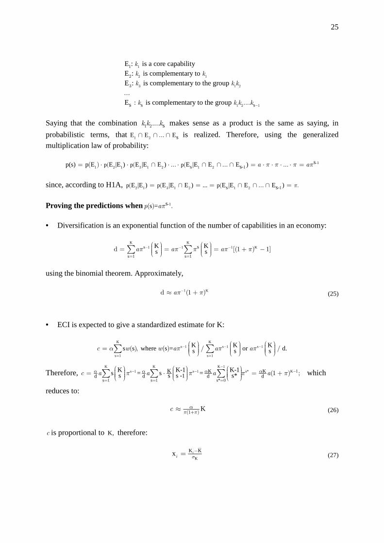
• Diversification is an exponential function of the number of capabilities in an economy:

K KK

s s

s sK Ks s

1 1 1

1 1

d (1 ) ][ 1a a aπ π π π π− − −

= =

= = = + − ∑ ∑

using the binomial theorem. Approximately,

K1d (1 )a ππ−≈ + (25)

• ECI is expected to give a standardized estimate for K:

s

K Ks s s

s

s s wher K K Ks =e os sr .s d1

1 1 1

1

( )( ), / /w aac aw π π πα − − −

= =

= ∑ ∑

Therefore, K

s*K K

s s K

s s s*d d

Kd d

KK1ss = s = s*

K K-1 K-1s s -

1

1 1

1 1

1

0

(1 ) ;c a a a aα α α αππ π π

−− − −

= = =

= ⋅ = +

∑ ∑ ∑

which

reduces to:

K(1 )

cπ πα+

≈ (26)

c is proportional to K, therefore:

K

K Kx i

i σ

−= (27)

26

We have simplified the model in section 4 to one unobservable parameter, namelyπ , by imposinga π= , thereby letting ss( ) ,p π= because the general insight conveyed by the predictions does not depend on a (which anyway cancels out in the second prediction). The limitation in doing so, however, is the fact that the probabilitya , as opposed toπ , could depend on K, and thus be country-specific. In this regard, a becomes an interesting parameter in itself, for it can be used to account for the differences in the endowment of countries in core capabilities, by assuming, for example, that represents the proportion of core capabilities in countryi : C K /Ki i ia a= = , where CK

i stands for the number of core capabilities in country i . This might shade light on issues like:

• the globalization and the “splicing up of the value chain”, due to the fact that more and more companies in the industrialized world have a tendency to concentrate on the “core” of their products and leave the rest for other companies offshore, particularly those of developing countries; therefore, a country may be counted among the exporters of a product, while in reality it did but “add some value” to the core,

• the specificity of natural-resource based economies where many western companies have based their equipment and other capabilities.

However, we leave these points as a lead for future investigations.

A.2 ECI and PCI as centrality measures

There is a parallel between ECI and PCI and the concept of eigenvector centrality. This metric indicates how important or central each node is within a network; it is computed as an eigenvector of the adjacency matrix representing the network. We would like to relate in what follows the concept of economic complexity to the eigenvector centrality literature. One can, from the outset, interpret diversification and ubiquity as centrality measures: they correspond to the degrees of the nodes (countries and products, respectively), and, as such, are degree-centrality measures.

Equations (11) and (12) read in matrix form

W W

or , where A== and x=W W* * Ax= x0 c c 0 c

0 s s 0 sλ λ

(28)

after assuming (without loss of generality) the same proportionality constant for both c and s,α β= , and letting, here, 1 1λ α β− −= = . The matrix A can be viewed as the adjacency matrix16 of the weighted and directed country-product bipartite network where a country i

16 Technical detail: the term “adjacency matrix” has been used previously in reference to the country-product matrix M. Strictly speaking, however, an adjacency matrix is a square matrix—like the matrix A in equation (28)

; the matrix M—like W for the matrix A—is only one of its two nonzero blocks, the other being TM — W* respectively. The zero blocks simply denote the fact that in a bipartite network, by definition, there is no direct

relationship between elements of the same nature ( and 0ija if i j= are both countries or both products). Some

authors use the term “biadjacency matrix” to refer to a matrix like M.

27

connects to a product j with the weight ijw (in the country-product direction), and the product

j connects to the country i with the weight jiw ∗ (in the product-country direction). From this,

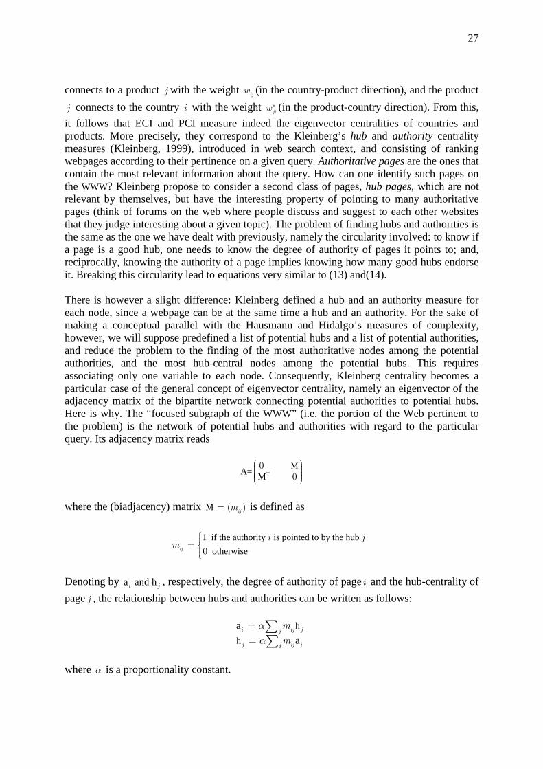
it follows that ECI and PCI measure indeed the eigenvector centralities of countries and products. More precisely, they correspond to the Kleinberg’s hub and authority centrality measures (Kleinberg, 1999), introduced in web search context, and consisting of ranking webpages according to their pertinence on a given query. Authoritative pages are the ones that contain the most relevant information about the query. How can one identify such pages on the WWW? Kleinberg propose to consider a second class of pages, hub pages, which are not relevant by themselves, but have the interesting property of pointing to many authoritative pages (think of forums on the web where people discuss and suggest to each other websites that they judge interesting about a given topic). The problem of finding hubs and authorities is the same as the one we have dealt with previously, namely the circularity involved: to know if a page is a good hub, one needs to know the degree of authority of pages it points to; and, reciprocally, knowing the authority of a page implies knowing how many good hubs endorse it. Breaking this circularity lead to equations very similar to (13) and(14).

There is however a slight difference: Kleinberg defined a hub and an authority measure for each node, since a webpage can be at the same time a hub and an authority. For the sake of making a conceptual parallel with the Hausmann and Hidalgo’s measures of complexity, however, we will suppose predefined a list of potential hubs and a list of potential authorities, and reduce the problem to the finding of the most authoritative nodes among the potential authorities, and the most hub-central nodes among the potential hubs. This requires associating only one variable to each node. Consequently, Kleinberg centrality becomes a particular case of the general concept of eigenvector centrality, namely an eigenvector of the adjacency matrix of the bipartite network connecting potential authorities to potential hubs. Here is why. The “focused subgraph of the WWW” (i.e. the portion of the Web pertinent to the problem) is the network of potential hubs and authorities with regard to the particular query. Its adjacency matrix reads

TM

A= M0

0

where the (biadjacency) matrix M ( )

ijm= is defined as

if the authority is pointed to by the hub

otherwise

1

0ij

i jm

=

Denoting by a and hi j , respectively, the degree of authority of pagei and the hub-centrality of

pagej , the relationship between hubs and authorities can be written as follows:

h

h

a

a i ij jj

j ij ii

m

m

α

α

=

=∑∑

where α is a proportionality constant.

28

This states simply that the degree of authority of a node is proportional to the sum of the hub-centralities of the pages pointing to it, and vice versa. Denoting by a and hthe vectors of authority and hub measures, respectively, these equations read in matrix form:

TM a a a

nd or , with h a h hM xAx x 100

.λ λ αλ − =

= = =

These equations and the ones in the previous case are equivalent. Indeed, the analogy between the two approaches is not only mathematical: as in the complexity framework, one can interpret the observable hub-authority bipartite network as the projection of the unobservable tripartite network connecting authorities to the information they contain, and hubs to the information they lead to. One cannot “observe” the latter network because the type of information contained on a webpage is not easily assessable beforehand. This analogy can be summarized as follows:

capabilities information

complex economies authoritive pages

sophisticate

↔

↔

d products hubs

problem: capabilities are not directly countable problem: information is not directly measurable

↔

↔

(limits of text-based ranking)

solution: indirect measure of complexity based solution: indirect measure of centrality based on

on the links of the country-product network the

↔

hub-autority links

A.3 The “method of reflections” and convergence

Originally, the authors defined ECI and PCI according to the following recursive process, which they refer to as the “method of reflections” (Hidalgo & Hausmann, 2009)17:

c

c

s

s1

1

in ij jnj

jn ji ini

w

w

−

∗−

=

=∑∑

under the initial conditions :

c (i.e. diversification)

(i.e. ubiquity)s0

0

i ijj

i iji

m

m

=

=

∑∑

After some iterations, the values of c and s are normalized to have ECI and PCI. The reason why we have adopted a slightly different formulation is that, as such, this iterative process converges to a multiple of the vector [1…1]T

; In other words, all countries and all products are

17 They use a different notation from the one adopted in this paper.

29

assigned an equal complexity, which is not meaningful. Therefore, the number of iterations to stop at seems arbitrary.

The study of this dynamical system is more easily done by writing it the following matrix form:

x =Ax1n n− (29)

-

-

Wx = x = , and where , A= W*

11

1

c c 0;

s s 0n n

n nn n

−

k kfor every k, c and s being respectively the vector

of economic complexities and product sophistications corresponding to the thk iteration. Equation (29) implies that

x =A x0.n

n (30)

To prove the convergence of Tto 1 ] 1x [n

… , it is convenient to write the initial conditionx0as a

linear combination of the eigenvectors of the matrix A, which we refer to as1 v ,...,vm

:

kk kvx =0

mα∑

(31)

We will suppose 1 v ,...,vm

to be associated with the eigenvalues1,...,

mλ λ , respectively, and

assume 1λ to be the dominant eigenvalue in absolute sense, so that 1v can also be called the

dominant eigenvector of A, i.e. the eigenvector associated with the dominant eigenvalue. Using (31) in (30) gives:

k k k k kk kv v / ) vx =

1 1 1 11(n n n

nα λ α λ λ λ

>+=∑ ∑

(32)

By the assumption that 1λ is the dominant eigenvalue, k kk

/ ) v 1 1

0( nλ λ>

→∑ as n → ∞ ;

therefore v x as 1 1 1n

n nα λ→ → ∞ . Because every column of the matrix A sums to 1

= =( 1)ij jij iw w∗∑ ∑ , the vector T1 1][ … is an eigenvector of A associated with the eigenvalue

1.

Finally, from the Perron-Frobenius theorem, which states that the dominant eigenvector of a non-negative matrix is the only positive eigenvector it has (omitting the trivial multiples thereof), we can conclude18 that T 1, v 1 1]

1 1[λ = = … and:

T1 1] x as 1[

nnα→ … → ∞ (33)

It is worth pointing out that this convergence holds for any initial conditions.

Later, the authors propose To take as ECI and PCI, the eigenvectors corresponding to the second largest eigenvalue of the matrix WW*, and W*W (Hausmann et al., 2011). These vectors correspond indeed to the eigenvector v2 of the matrix A, since A

and its square

18 Assuming that the country-product network is a “connected” one.

30

2 0 WW* 0

A =W*W

have the same eigenvectors. Because one can come to the same eigenvectors using a more direct definition like the one given by equations (7) and (8), we have avoided this iterative method in section 3.