on the determinants of fiscal centralization: theory and ...staff.aub.edu.lb/~ugo/pap.pdf ·...
TRANSCRIPT

Journal of Public Economics 74 (1999) 97–139
On the determinants of fiscal centralization: Theory andevidence
*Ugo PanizzaOffice of the Chief Economist, Inter-American Development Bank, Stop W-0436,
1300 New York Avenue NW, Washington DC 20577, USA
Received 1 April 1998; received in revised form 1 September 1998; accepted 1 December 1998
Abstract
This paper presents a simple model that unifies most of the results of the literature onfiscal federalism. The model describes an economy characterized by two levels ofgovernment, one public good, and a private good. The predictions of the model are testedby using a new set of measures of fiscal centralization. The main findings are that countrysize, income per capita, ethnic fractionalization, and level of democracy are negativelycorrelated with the degree of fiscal centralization. The model is tested using OLS, Tobit,and semi-parametric estimators. The paper also shows that the variables included in theregression are helpful in the prediction of changes in the level of centralization. 1999Elsevier Science S.A. All rights reserved.
Keywords: Political economy; Median voter; Fiscal federalism; Decentralization
JEL classification: D720; H110; H710; H770
1. Introduction
Across countries we observe very different institutional arrangements and verydifferent levels of fiscal centralization. The recent years have witnessed strongmovements toward decentralization and secession (Argentina, Colombia, Ethiopia,the republics of the former Soviet Union, Yugoslavia, India, Czechoslovakia,
*Tel.: 11-202-623-1427; fax: 11-202-623-2481.E-mail address: [email protected] (U. Panizza)
0047-2727/99/$ – see front matter 1999 Elsevier Science S.A. All rights reserved.PI I : S0047-2727( 99 )00020-1

98 U. Panizza / Journal of Public Economics 74 (1999) 97 –139
Canada, Belgium, Italy and Spain). At the same time, a divided country hasreunified (Germany), large free-trade zones have been created, and there have beenimportant steps towards the economic and monetary union of some Europeancountries. It is therefore natural that decentralization has been at the center of thepolitical and economic debate in many countries.
This paper attempts to identify empirical regularities explaining cross-countrydifferences in the level of fiscal centralization. To set the stage for the empiricalwork, Section 2 presents a stylized model describing an economy with two levelsof government, one public good, and one private good. The central governmentobtains utility from the size of its budget and the equilibrium level of centraliza-tion is determined by a sequential game where the central government moves first.
The key findings of the theoretical model are that the level of fiscal centraliza-tion is inversely correlated with: (i) country size; (ii) income per capita; (iii) tastesdifferentiation; and (iv) level of democracy. The last point is particularlyinteresting because it may account for the wave of decentralization that hasfollowed the end of the Cold War.
The existing literature on fiscal centralization can be divided into three mainbranches. The first branch studies the optimal division of powers between thecentral and local governments (Musgrave, 1959; Oates, 1972). One of the mainresults of this branch of the literature is the Decentralization Theorem (Oates,1972) that identifies the conditions under which it is more efficient for localgovernments to provide the Pareto-efficient levels of output for their respectivejurisdictions than for the central government to provide an uniform level of outputacross all jurisdictions. One of the corollaries of the decentralization theorem isthat the benefits of decentralization are positively correlated with the variance indemands for publicly provided goods. This is also one of the key results of themodel presented in Section 2.
The second branch of the literature concentrates on the role of organizationcosts (Breton and Scott, 1978). A decentralized system can reduce mobility andsignaling costs, but it is likely to increase administrative and coordination costs.The optimal level of decentralization is the one that minimizes the sum of thesecosts.
The third branch of the literature emphasizes the benefits of competition amongjurisdictions. Tiebout (1956) studies how, in a system with many jurisdictions, theagents can ‘vote with their feet’ and locate in the jurisdiction that has policies thatare closer to their preferences. While Tiebout concentrates on horizontal competi-tion, Breton (1996) studies the benefits of vertical competition. According to thisnotion, different levels of government, in an effort to increase their ‘market share,’provide the citizens with the optimal type and quantity of public goods. Brennanand Buchanan (1980) claim that horizontal and vertical competition amongdifferent levels of government can be very important in containing the size of theirbudgets.
In addition to the fiscal federalism literature, the scope of this paper extends to

U. Panizza / Journal of Public Economics 74 (1999) 97 –139 99
several issues examined in the recent strand of political economy literature thatstudies the optimal number and size of nations (Alesina and Spolaore, 1997) andthe optimal amount of public goods in countries with heterogeneous preferences(Alesina et al., 1996a,b). The model presented in this paper constitutes a step in thedirection indicated by Alesina and Spolaore (1997) who suggest that it would beinteresting to extend their analysis to a framework with multiple levels ofgovernment. The presence of two levels of government is the key differencebetween the model presented in this paper and the one studied by Alesina andSpolaore (1997); Alesina et al. (1996a).
The second part of the paper builds a new data set of measures of fiscalcentralization and uses it to test the predictions of the model. The theory is testedusing both standard techniques (OLS and Tobit) and a semi-parametric estimatorthat does not require normally distributed residuals. To the best of my knowledge,Oates (1972); Wallis and Oates (1988) are the only two attempts to use a large setof cross-section data to study the existence of empirical regularities explainingdifferences in centralization across countries. Oates (1972) finds that only size andincome per capita are significantly correlated with fiscal centralization. Wallis andOates (1988) study the fiscal structure of the American states. They build a panelof state-level measures of fiscal centralization and find a correlation between a fewsocio-economic variables (the percentage of urban population, the percentage ofwhites, and the percentage of farmers) and fiscal centralization. When Wallis andOates test the model using a simple cross section of American states they find thatonly size is robustly associated with fiscal centralization.
In the light of the existing literature, the results of this paper seem particularlyinteresting. In fact, the empirical analysis identifies a correlation between fiscalcentralization and two variables measuring the degree of democracy and thedegree of ethnic fractionalization. These results are consistent with the model ofSection 2 and contradict the idea that it is impossible to find a unique set ofvariables to explain cross-country differences in fiscal centralization (Oates, 1972).
2. A model of fiscal centralization
The model presented in this section extends the framework developed byAlesina and Spolaore (1997); Alesina et al. (1996a), to an economy with twolevels of government. The model studies a linear country with area S, population
1N, and divided into J jurisdictions. S, N and J are assumed to be exogenous. Tosimplify the analysis, J is assumed to be an odd number.
Since it is not possible to capture in a single model the richness of the vastliterature on fiscal centralization, the focus of the model presented in this section is
1 Alesina and Spolaore (1997) present a model where the size and number of countries isendogenous but the size of the public good is exogenous.

100 U. Panizza / Journal of Public Economics 74 (1999) 97 –139
simplification and unification. Having a unified framework will be useful toorganize the ideas and guide the empirical analysis presented in Section 4.
The government produces one public good: G (for government). The general(local plus central) government budget constraint is given by T 5 G, where Tstands for tax receipts. This can be written in per capita levels as: t 5 g. Per capitaconsumption of the private good is defined by c. The prices of all goods arenormalized to 1. All individuals have the same income y, on which they pay alump sum tax t, and similar preferences, but they differ in their tastes for the type
2of public good. Education is an example of publicly provided good on whichpreferences are often polarized: some citizens may prefer religious as opposed tosecular schools or may favor the use of a specific language. It is assumed that theindividuals are uniformly distributed over the territory and that the individuals arestratified and sorted according to their preferences for the public good. The latterimplies that there is a one-to-one correspondence between the physical and the‘ideological’ distance from the center of the country. The theoretical basis for thisassumption is provided by the literature pioneered by Tiebout (1956). Accordingto this literature, individuals with similar preferences tend to locate in the samecommunity and stratification is an equilibrium condition. The model of this paperassumes a situation where Tiebout-style stratification has already taken place and,since individuals are already sorted according to their preferences, there is no rolefor mobility.
Although there is no general consensus supporting the Tiebout hypothesis, manyempirical studies have found a strong support for neighborhood stratification inAmerican cities (Hamilton et al., 1975; Borjas, 1995). The idea that individuals aresorted according to their preferences is also central in Alesina and Spolaore’swork. These authors claim that: ‘‘If there were no relationship between locationand preferences, then there would be no presumption that a country would begeographically connected’’ (Alesina and Spolaore, 1997, p. 1030).
The preferences of the ith citizen are described by a distance-sensitive utilityfunction (Jurion, 1983):
12a (u l 1(12u )l ) bim ijU 5 g c (1)i i i
where g is the per capita amount of government expenditure, l representsim
individual i’s distance from the center of her country, l the distance from theij
center of the jurisdiction, and u the level of centralization (i.e. the share of thepublic good that is provided by the central government). The difference in tastesacross individuals is captured by a [[0,1]: a 50 indicates a country with a veryhomogeneous population, while a 51 characterizes a country with a population
2 The assumption of homogeneous income allows us to abstract from all the issues linked to incomeredistribution. Wildasin (1991) discusses in great detail the cost and benefits of local versus centralredistribution.

U. Panizza / Journal of Public Economics 74 (1999) 97 –139 101
with diversified tastes. Hence, a(ul 1(12u )l ) is the distance between in-im ij
dividual i’s preferred type of government and the actual type of governmentprovided in equilibrium. Assuming that S[(0,1) guarantees that the exponents inEq. (1) are non-negative for all individuals.
It is easy to show that the above utility function generates the prediction that thecloser an individual’s preferences are to the actual government the higher is theratio between public and private goods that the individual will demand. Thisintuitive result justifies the use of a utility function like the one in Eq. (1). Not allthe utility functions would generate this prediction. A simpler Cobb-Douglas
g butility function of the kind: U 5[g (12a(ul 1(12u )l ))] c would generatei i im ij i
the non-realistic prediction that all individuals demand the same mix of public andprivate goods, no matter what their preferences for the type of public good are. Allthe results obtained in this paper can be reproduced using the additive utilityfunction studied by Alesina et al. (1996a).
By maximizing the utility function of Eq. (1) under the constraint y5c1g, it ispossible to derive the following demand functions for the public and privategoods:
d yi]]g 5 (2)i d 1 bi
by]]c 5 (3)i d 1 bi
with d 512a(ul 1(12u )l ). Note that ≠g /≠d .0, ≠c /≠d ,0. As alreadyi im ij i i i i
pointed out, each citizen will have different preferences for the quantity of g and c.The actual level of g provided in equilibrium will then be determined by voting.
Note that the idea behind Eq. (1) is that utility is decreasing in the distance fromthe type of public good provided in equilibrium (i.e. that U . 0). Since U 5d di iiU d ln( g), this condition will be satisfied only if g.1. It is then necessary toi
assume that g.1. Since d .0, this assumption only requires an appropriatei
definition of the units in which y is measured.To derive the equilibrium level of centralization I assume that the central
government is the first mover and decides the level of centralization. Thisassumption may seem at odds with democratic voting over the type and amount ofpublic good. Its theoretical background relates to the large political scienceliterature that shows how the agenda setter can, by controlling the order of voting,
3manipulate the final outcome of an election. The agenda setter has always somepower and, in the model presented in this paper, the level of democracy measureshow much of this power the government is willing to use to achieve its own goals.
3 One of the most important results in this literature is McKelvey (1976) Chaos Theorem. The lattershows that multidimensional voting is almost always characterized by a situation with no Condorcetwinner.

102 U. Panizza / Journal of Public Economics 74 (1999) 97 –139
After observing u, the citizens vote on the amount of the public good, and thenon the type of the public good. The assumption of sequential decision making(similar to the one used by Alesina et al., 1996a) reflects the budget processadopted in many countries (Alesina and Perotti, 1996).
In a democratic system the type of public good provided is the one preferred bythe median voter. Two types of median voters will be considered: the ‘national’median voter, indicated by med, and the median voter of jurisdiction j, indicatedby mej. Given the assumption on the spatial distribution of individuals, the medianvoters will be located at the center of the country and at the center of their
4jurisdictions, respectively. See Fig. 1.At this point it is necessary to investigate who will assume the role of ‘central
government.’ On principle, anybody who promises to supply the type of publicgoods preferred by the median voter could play the role of central government, butonly one individual can credibly commit to provide such type of public good: themedian voter herself. Any other individual will, once elected, have an incentive todeviate and implement a policy closer to her own preferences. It is thereforenatural to assume that the central government will have preferences for the publicgood identical to those of the national median voter. Besides sharing thepreferences of the national median voter, the central government derives additionalutility from staying in power. Following Brennan and Buchanan (1980) view ofthe central government as a budget-maximizing Leviathan I will assume that theutility that the government obtains from staying in power is a function of thebudget it controls.
The central government chooses u in order to maximize the following utilityfunction:
medV 5 fU 1 (1 2 f)ug (4)gov
Where f [(0,1) indicates the level of democracy: f 50 indicates a dictatorship,while f 51 indicates a perfectly democratic country. The utility function of Eq.(4) has a straightforward interpretation: dictators only care about their budgetwhile democratic governments identify their preferences with the preferences of
Fig. 1. A country with five jurisdictions.
4 The assumption that j is an odd number guarantees that the national median voter is also themedian voter of the central jurisdiction.

U. Panizza / Journal of Public Economics 74 (1999) 97 –139 103
the median voter. Given the discretional power of the agenda setter, the centralgovernment will always be able to extract some rent. In the utility function of Eq.(4) the level of democracy measures how much of this rent the central government
5is willing to extract.Notice that the probability of being re-elected does not appear in the govern-
ment’s utility function. This is because, given the structure of preferences, themedian voter is the only individual for which the Condorcet winning policy isincentive compatible. Therefore she will be re-elected with probability 1.
For the central government the distances from both the center of the jurisdictiongov band the center of the country are 0. Eq. (2) can then be rewritten as: V 5fgc 1
(12f)ug.The government maximizes Eq. (4) by solving the model backward. The last
decision (and therefore the first to analyze) is on the type of the public good. Thetype of public good chosen in equilibrium is the one preferred by the median voter(and therefore the central government).
The next step is to determine the amount of the public good to be provided inequilibrium. By applying the median voter theorem and using the demand functionof Eq. (2) it is possible to derive the following:
Proposition 1. The amount of public good provided in equilibrium is given by:
my]]g* 5 (5)m 1 b
S S] ]F Gwith m 5 1 2 a u 1 (1 2u ) .4 4J
Proof. See Appendix A.
In a model with only one level of government, Alesina et al. (1996a) show thatthe optimal quantity of public good depends on the ‘median distance from themedian.’ In the framework presented here, it is possible to interpret (u(S /4)1
(12u )S /4J) as a weighted average of the median distance from the nationalmedian and the jurisdiction median and (12m) as the ‘ideological’ distance fromthe median. The latter will be close to 0 if a country is very small or if itspreferences are homogeneous, and close to 1 for large countries with heteroge-neous preferences.
By substituting Eq. (5) into the central government’s utility function Eq. (4), itis easy to show that the central government will choose the value of u thatmaximizes the indirect utility function:
5 This could also be interpreted as: ‘Given the institutional structure, how much rent is the centralgovernment capable of extracting.’ This would involve modeling the institutional structure and goesbeyond the scope of this paper.

104 U. Panizza / Journal of Public Economics 74 (1999) 97 –139
bmy by my]] ]] ]]V 5 f 1 (1 2 f)u (6)S DS Dgov m 1 b m 1 b m 1 b
From the maximization of Eq. (6) it is possible to derive the following:
Proposition 2. The amount of fiscal centralization u is decreasing in: (i) the levelof taste differentiation a; (ii) democracy f; (iii) income per capita y; and (iv)country size S.
Proof. See Appendix B.
The proof of Proposition 2 is simple but long and tedious. Its interpretationhowever is straightforward. Since (i) the central government obtains direct utilityfrom the size of its budget, and (ii) d 51.m, the amount of public goodgov
demanded by the government is greater than g*. In other words, voters force thecentral government to decentralize by choosing an amount of publicly providedgood lower than the amount preferred by the central government. To increase theamount of public good produced in equilibrium the central government is thenrequired to reduce the level of centralization. Eq. (14) in Appendix B shows thatthe central government chooses the value of u that sets the marginal cost ofcentralization (due to the fact that g ,0) equal to the marginal benefit ofu
centralization (due to the fact that, for a given level of g, an increase in u increasesthe government budget). Since the ideological distance from the center (12m)depends on the size of the country and on the level of heterogeneity of preferences,it is easy to show that g ,0 and g ,0. Therefore, an increase in the level ofa S
tastes differentiation or in country size will decrease the amount of public goodand the marginal benefits from centralization. A decrease in g by increasing
gov govU /U will also increases the costs of centralization. Both effects will induceg c
the central government to reduce the level of u.One of the results of Proposition 2 is in line with Alesina and Spolaore (1997)
finding that democratization should be positively correlated with the equilibriumnumber of countries and it proves the claim that their analysis can be applied tothe division of a country into jurisdictions. A corollary to Proposition 2 is that a
6perfectly democratic government will set u 50 (see the proof in Appendix B).Proposition 2 does not provide any result for the effect on centralization of the
number of jurisdictions J. A change in the number of jurisdictions will have twoopposite effects. On the one hand, an increase (decrease) in the number ofjurisdictions will affect m and cause an increase (decrease) of g and therefore ofthe benefits (from the central government’s point of view) of centralization. On the
6 This result allows to compare the model of this paper with the normative analysis. In fact, it ispossible to show that, given the preferences illustrated in Eq. (1), a perfectly democratic governmentwill behave like a Benthamite social planner (this is proved in Appendix B).
U. Panizza / Journal of Public Economics 74 (1999) 97 –139 105
other hand, since g ,0, an increase in J will increase the centralization-elasticityuJ
of the demand for g and therefore the cost of centralization. The final effect on theequilibrium level of centralization will depend on which of these factors dominatesthe other.
3. Taking the model to the data
Proposition 2 generates four predictions. The result that ≠u /≠a ,0 suggests thatcountries with polarized preferences for the type of public good should be moredecentralized than countries with homogeneous preferences. In countries withhomogeneous tastes the central government can induce the citizens to vote for ahigh level of expenditure in publicly provided good even when the latter are
7provided in a highly centralized fashion. Hence, we should find a negativecorrelation between the level of centralization and heterogeneity in thedemand of public goods.
Economic theory indicates that the key factors in determining demand are tastesand income. Since the model assumes constant income, I will concentrate on therole of taste heterogeneity. The problem in testing the possible presence of anegative correlation between centralization and taste heterogeneity is how tomeasure the latter. In Section 3.1 I provide some justifications for the use of ethnicfractionalization as a proxy for taste heterogeneity.
The result that ≠u /≠f is based on the idea that a democratic government willnot try to exploit its agenda setter power. Hence, we should find a negativecorrelation between the level of democracy and the degree of centralization.This results, besides being in line with Alesina and Spolaore (1997) who find thata world of dictatorships would lead to larger countries, is also consistent with Adesand Glaeser’s (1995) finding that dictatorships tend to have very large capitalcities.
The central government’s utility function suggests that perfect democraciesshould set u 50 and very repressive dictatorships should set u 51. The majority ofcountries included in the data set used in this paper fall between these twoextremes. Most of the real-world governments are neither perfect democracies(because they are run by self-interested politicians with some agenda-settingpower) nor perfect dictatorships (even dictators need to rely on the support of thegroup of people who put them in power). It should also be noted that, since somepublic goods cannot be efficiently produced by the local governments (these aregoods with large spillover; defense is an example of such a good), even perfectdemocracies will have levels of centralization greater than 0.
govU g7 ]Remember that, in equilibrium, . 1 and therefore the Central Government would like togovU c
increase public good expenditure above its equilibrium level.

106 U. Panizza / Journal of Public Economics 74 (1999) 97 –139
The result that ≠u /≠y,0 is based on the idea that decentralization is a normalgood. Hence, we should find a negative correlation between centralization andincome per capita. The existing literature does not agree on the relationshipbetween income per capita and fiscal centralization. Some authors claim thatdecentralization is a luxury and therefore should be positively correlated withincome per capita (Wheare, 1964). In support of this idea Oates (1972) finds thatthe level of fiscal centralization is inversely correlated with a country’s level ofdevelopment. Other authors have observed that this relationship tends to disappearwhen only rich countries are examined. Wallis and Oates (1988), for instance,show that in developed countries centralization is positively correlated withincome per capita. A possible explanation for this finding is that richer countriestend to have more generous redistributive policies, usually implemented by thecentral government. Casual evidence indicates that some rich countries areextremely decentralized (Switzerland, United States, Canada are examples) whileothers are highly centralized (France for instance). The regression analysis ofSection 4 indicates a strong correlation between income per capita and decentrali-zation.
The result that ≠u /≠S,0 depends on the fact that, other things equal, the biggerthe country, the smaller m (leading to a large ideological distance from the center(12m)), and hence the quantity of g provided in equilibrium. The central
gov govgovernment will then be forced to decentralize in order to reduce the U /Ug c
ratio. Hence, we should find a negative correlation between centralization andcountry size. While casual evidence shows that there are some countries thatcontradict this prediction (Switzerland is more decentralized than France forexample), the regression analysis provides strong support for a negative correlationbetween size and centralization.
The empirical analysis uses Area as the relevant measure of size. Support forusing this variable can also be found in the previous fiscal federalism literature.The latter suggests that the benefits of decentralization can be offset by marketfailures. The most important of these market failures relates to the presence ofspillovers across jurisdictions. These externalities are likely to be inverselycorrelated with the size of the jurisdictions. So, to the extent that larger countries
8have larger jurisdictions, land area (Area) will be an appropriate proxy for size.Note that the utility function of the central government (Eq. (4)) depends on the
medper capita level of expenditure in g. By changing Eq. (4) into V 5fU 1(12gov
f)uG (i.e. considering total government expenditure rather than per capitaexpenditure), it would be possible to show that centralization is increasing in
9population size (≠u /≠N.0).
8 Switzerland is a notable exception. The small size of its jurisdictions is compensated bycharacteristics of the territory that limit the mobility of its citizens, and therefore the spillovers amongjurisdictions.
9 Tables 13 and 14 show a positive (but not statistically significant) correlation between populationand centralization.

U. Panizza / Journal of Public Economics 74 (1999) 97 –139 107
Summarizing, the simple framework presented in this section predicts a negativecorrelation between fiscal centralization and: (i) taste heterogeneity; (ii) demo-cracy; (iii) income per capita; and (iv) country size.
Note that the predictions of Proposition 2 derive from the reduced form of themodel of Section 2. Estimating the structural form of the model would require anequation for the behavior of the agents and one equation for the behavior of thecentral government. This could be done by estimating the following simultaneousmodel:
g 5 a 1 a y 1 a Fract 1 a Area 1 a u 1 u (7)i 1 2 i 3 i 4 i 5 i i
u 5 b 1 b Dem 1 b y 1 b g 1 v (8)i 1 2 i 3 i 4 i i
Eq. (7) estimates the quantity of public good voted by the economic agents. Theequation is identified by the exclusion of the democracy variable (Democracy doesnot appear in the demand functions of Eqs. (2) and (3)). Eq. (8) estimates the levelof centralization chosen by the central government. The equation is identified bythe exclusion of Area and Fract, variables that do not enter in the direct utilityfunction of the central government. The theoretical model predicts a positive signfor a and b and a negative sign for all the other coefficients.2 4
The above model is fully identified and could be estimated using two-stage leastsquares. Unfortunately, TSLS produce consistent but inefficient estimates and,
10with approximately 55 observations, this could be a serious problem. Theempirical part of the paper will then concentrate on estimating a reduced formequation of the kind u 5f( y, Area, Fract, Dem).
One last problem concerns the technique used in estimating the model. Bydefinition, the level of fiscal centralization cannot be higher than 100%. Therefore,I am dealing with a censored dependent variable and, assuming well-behavedresiduals, the appropriate estimation technique is the Tobit model. It should bepointed out that Eq. (4) shows that the central government will set u 5100 only iff 50. Hence, only very repressive dictatorships should be fully centralized. Thedata seem to support this implication. If we exclude very small countries where thescope for decentralization may be extremely limited (Malta and Singapore, forinstance), we observe that full centralization is found almost only in extremelyautocratic regimes like Myanmar and Zaire (Egypt is an exception).
3.1. Data
What follows discusses the variables used in the empirical analysis. Adescription of the data sources can be found in Appendix C.
10 The parameters obtained by estimating Eqs. (7) and (8) with TSLS have all the expected signs butthey are not statistically significant. The estimation results are available upon request.
108 U. Panizza / Journal of Public Economics 74 (1999) 97 –139
3.1.1. Fiscal centralizationTo test the predictions of the model studied in Section 2 it is necessary to build
a data set of measures of fiscal centralization. Identifying such measures is not aneasy task. The main issue is finding a method to quantify the activity of localgovernments that results from independent decision making. Oates (1972)discusses the conceptual problems involved in the choice of the right measure offiscal centralization. These problems can be summarized as follows: (i) Differentlevels of local governments should be weighted in different ways. For instance,large regional governments should be considered more centralized than smaller,city-wide, governments. (ii) Sometimes the local governments collect revenues ormake expenditure but have no autonomy in deciding the tax amount to becollected or the type of expenditure to be made. This problem is also related to theidentification of the relevant definition of jurisdiction. (iii) The role of inter-governmental grants.
The available data do not allow to address the problems listed above. Theydivide between the central government and local governments as a group.Information on the appropriate decision units and on the use of the inter-governmental grants is not available. It is therefore impossible to apply aweighting scheme to different levels of local governments or identifying thenumber of relevant jurisdictions.
Following Pryor (1968), I define centralization ratios as the percentage ofrevenues (or expenditure) of the central government out of the total revenues (orexpenditure) of the public sector. Two measures of fiscal centralization (TotalRevenues and Total Expenditure) for 1975, 1980 and 1985 are built using data
11from the IMF (1975, 1980 and 1985) Government Finance Statistics Yearbook.The centralization ratios are illustrated in Table 8 of Appendix C. While the data
for 1980 and 1985 are very similar (the correlation between the 1980 and 1985values is 0.95 for total revenues and 0.98 for expenditure) the centralization ratiosfor 1975 are less correlated with the 1980 and 1985 values (the correlation isbetween 0.6 and 0.75). This may be an indication of either a change in the level ofdecentralization or a change in the methods of data collection.
Oates (1972) tested for the determinants of fiscal centralization using the datareported in the World Tables (The World Bank, 1969). These data, following theUnited Nations accounting conventions, include social security programs in totalpublic sector revenues and expenditures, but do not include social securityprograms in the revenues or expenditure of the central government. Given the factthat in some countries social security programs represent a big share of thegovernment budget (sometimes more than 30%), not including social security
11 Until 1988 the IMF provided information on central governments expenditure and revenues and ongeneral governments (defined as central plus local governments) expenditures and revenues. Thecentralization ratios are computed by dividing the former by the latter. A detailed description of themethod used to build the data is provided in Appendix C.

U. Panizza / Journal of Public Economics 74 (1999) 97 –139 109
programs makes a big difference. Therefore, the centralization ratios reported bythe World Tables are much lower than the centralization ratios used in this paper.Since the central government plays a very important role in deciding the size andthe scope of social security programs, the measure of fiscal centralization used inthis paper should be better suited for a study of the determinants of fiscal
12centralization than the centralization ratios of the World Tables.For most measures Yugoslavia is the most decentralized country. Among the
industrialized countries Switzerland, Canada, and the United States are the mostdecentralized. The values for Yugoslavia are suspiciously low. The shares of thefederal government in total revenues and expenditures are always below 30%.Although Yugoslavia was a well known case of extreme federalism the abovevalues may be the outcome of an accounting procedure that did not reflect theactual division of powers between the central and local governments.
3.1.2. Heterogeneity in the preferences for public goodsSince tastes are not directly observable, it is necessary to find a proxy for this
variable. It is not unlikely that different ethnic groups may diverge in their tastesfor publicly provided goods (education is an important example). Therefore,differences in tastes may be proxied by a measure of ethnic fractionalization(Fract). The possibility of a relationship between ethnic fractionalization andtastes was first explored by Oates (1972) who used a dummy variable to
13differentiate homogeneous from heterogeneous countries.One problem with Oates’ analysis is that a dummy variable dividing the world
between homogeneous and heterogeneous countries is a very coarse measure oftastes differentiation. A continuous measure of heterogeneity would be moreinstructive.
To address this problem, I measure ethnic fractionalization using the datacollected by the Department of Geodesy and Cartography of the State GeologicalCommittee of the Soviet Union, originally published in the Atlas Narodov Mira(1964) and then reported by Taylor and Hudson (1972). This variable ranges from0 (Korea) to 0.9 (Zaire) and measures the probability that two randomly selected
14individuals will belong to different ethno-linguistic groups. The same measurehas been used in cross-country studies of growth by Canning and Fay (1993);Mauro (1995); Castilla (1996); Easterly and Levine (1997). Easterly and Levinestudy the relationship between this measure of ethnic diversity and similar indicesproposed by various authors and find that ethnic fractionalization is a robust
12 Ideally, one should use data for the activities that are decentralizable and therefore exclude defenseand social security.
13 He used three measures of differentiation: linguistic, racial, and religious. These dummies assumeda value of 1 for countries that Oates deemed to be homogeneous and 0 for countries deemed to beheterogeneous.
14 The value for Korea was not included in the original data set of the Atlas Narodov Mira butreported (using a different source) by Taylor and Hudson (1972).
110 U. Panizza / Journal of Public Economics 74 (1999) 97 –139
predictor of potential ethnic conflicts. Alesina et al. (1996a) use ethnic fractional-ization to capture conflicts among groups in the decision of the quantity and typeof public goods. To support this idea, they quote a vast sociological literature thatfinds that preferences and conflicts over public policies are more stronglycorrelated with ethnic as opposed to income differences.
Most African countries are highly ethnically fractionalized and nine out of theten most fractionalized countries are in Africa (the tenth one is India). Zaire,Cameroon, South Africa, Nigeria, Central African Republic, Kenya and Zambiahave measures of ethnic fractionalization greater than 0.8. Among the industrial-ized countries, Canada has the highest degree of ethnic fractionalization (0.75),followed by Belgium (0.55), Switzerland, and the USA (0.5). Yugoslavia is theEuropean country with the highest degree of fractionalization (0.75).
Of course, ethnic fractionalization is appropriate to test the model of Section 2only if one assumes that the different ethnic groups are spatially separated. Supportfor this assumption comes from the empirical literature aimed at testing Tiebout(1956) model. It is also often observed that different ethnic groups are located indifferent regions of a country and, in some cases, these regions have large
15autonomy from the central government.
3.1.3. DemocracyTo test for the fourth hypothesis I use the data on political rights assembled by
16Gastil (1990). Gastil’s classification assigns the value 1 to perfect democraciesand 7 to countries where most citizens have no political rights. Following Barro(1996), I transform Gastil’s 1–7 ranking into a 0–1 ranking, where 0 correspondsto Gastil’s 7 and 1 corresponds to Gastil’s 1. An alternative source of measures ofdemocracy is provided by the Polity II data set (Gurr et al., 1989). The resultsobtained using the Polity II indices of democracy are essentially identical to theresults obtained using Gastil’s definition.
4. Estimations of the determinants of fiscal centralization
This section discusses the methods used to test for the empirical predictionsdescribed in Section 3.1. The results of the various tests are presented using thecentralization ratios for both government revenues and expenditures. As a first
15 A possible interpretation is that the central government ‘bribes’ ethnically diverse regions bygiving them more autonomy. For instance, in a highly centralized country like Italy there are fivespecial regions that enjoy large fiscal autonomy and transfers from the central government. Two ofthese regions are islands (Sardinia and Sicily). The other three are border regions characterized by largeethnic minorities: French in Valle d’Aosta, German in Trentino Alto Adige, and Slavic in Friuli VeneziaGiulia. Similar examples can be found in Canada, Belgium, India, Spain, Switzerland and the UK.
16 Gastil uses the following definition: ‘‘Political rights are rights to participate meaningfully in thepolitical process. In a democracy this means the right of all adults to vote and compete for publicoffice.’’

U. Panizza / Journal of Public Economics 74 (1999) 97 –139 111
step, the model is estimated using ordinary least squares. Then, more appropriateTobit and semi-parametric estimation methods are used.
Previous work found evidence for the fact that size and income per capita havesome weight in explaining fiscal centralization, but most attempts of finding anycorrelation between fiscal centralization and socio-political variables have not beensuccessful. I start the analysis by estimating two regressions where measures ofethnic fractionalization and democracy are added, one at a time, to a basicspecification that includes income per capita and area (these variables are alwaysincluded given the existing evidence of their correlation with centralization).Formally, I estimate linear forms of the following two equations: CENTR5f(Size,y, Fract), and CENTR5f(Size, y, Dem). The rationale for the above specificationsis to compare the effects on centralization of ethnic fractionalization anddemocracy. Next, I test the following equation:
CENTR 5 a 1 a Size 1 a y 1 a Fract 1 a Dem 1 u (9)i 0 1 i 2 i 3 i 4 i i
Instead of levels, the estimations use the logs of Area and GDP per capita. The logspecification improves the fit of the regression and indicates the presence of anon-linear relationship between these two variables and fiscal centralization.
Oates (1972) uses ordinary least squares to estimate an equation similar toCENTR5f(Area, y, Fract). Since the centralization ratios cannot be higher than100, the independent variables are censored from above and OLS is not theappropriate technique to estimate Eq. (9). It is well known that, with censoreddata, least squares estimates are biased. Greene (1993) finds that the bias isproportional to the percentage of limit observations. In the data set used in thispaper the non-limit observations range between 84 and 90% of the total. Thereforethe OLS estimates should have a bias that ranges between 10 and 20%.
Despite its fundamental flaw, I run OLS regressions to compare my results withOates’ work. The results, reported in Appendix D, confirm Oates’ finding that sizeand income per capita are negatively correlated with fiscal centralization. I alsofind that, as predicted by the model of Section 2, democracy and ethnicfractionalization are negatively correlated with fiscal centralization. These pre-liminary results, although not very strong (because the coefficients are not alwaysstatistically significant), are encouraging. Oates (1972) found that only size andincome had a role in explaining centralization and that the proxies for demand
17differentiation always had the wrong signs.
4.1. Tobit estimations
This section uses the Tobit model to test the predictions of Section 3.1. TheTobit model is the standard technique used to estimate equations with censored
17 In his regressions ethnic fractionalization was never statistically significant and always positivelycorrelated with centralization.
112 U. Panizza / Journal of Public Economics 74 (1999) 97 –139
dependent variables. The assumption of normally distributed residual is crucial forthe consistency of the Tobit estimates.
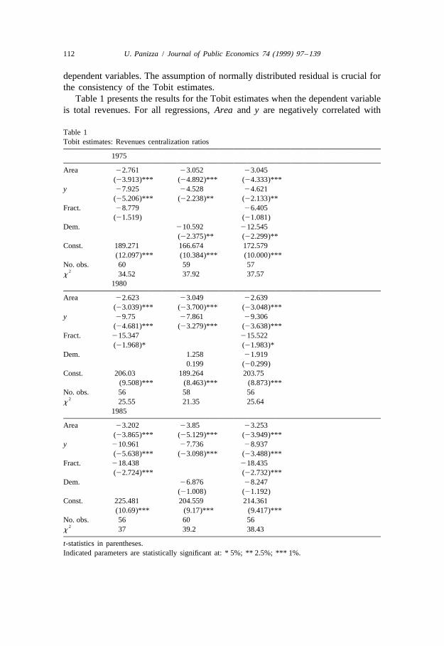
Table 1 presents the results for the Tobit estimates when the dependent variableis total revenues. For all regressions, Area and y are negatively correlated with
Table 1Tobit estimates: Revenues centralization ratios
1975
Area 22.761 23.052 23.045(23.913)*** (24.892)*** (24.333)***
y 27.925 24.528 24.621(25.206)*** (22.238)** (22.133)**
Fract. 28.779 26.405(21.519) (21.081)
Dem. 210.592 212.545(22.375)** (22.299)**
Const. 189.271 166.674 172.579(12.097)*** (10.384)*** (10.000)***
No. obs. 60 59 572
x 34.52 37.92 37.571980
Area 22.623 23.049 22.639(23.039)*** (23.700)*** (23.048)***
y 29.75 27.861 29.306(24.681)*** (23.279)*** (23.638)***
Fract. 215.347 215.522(21.968)* (21.983)*
Dem. 1.258 21.9190.199 (20.299)
Const. 206.03 189.264 203.75(9.508)*** (8.463)*** (8.873)***
No. obs. 56 58 562
x 25.55 21.35 25.641985
Area 23.202 23.85 23.253(23.865)*** (25.129)*** (23.949)***
y 210.961 27.736 28.937(25.638)*** (23.098)*** (23.488)***
Fract. 218.438 218.435(22.724)*** (22.732)***
Dem. 26.876 28.247(21.008) (21.192)
Const. 225.481 204.559 214.361(10.69)*** (9.17)*** (9.417)***
No. obs. 56 60 562
x 37 39.2 38.43
t-statistics in parentheses.Indicated parameters are statistically significant at: * 5%; ** 2.5%; *** 1%.

U. Panizza / Journal of Public Economics 74 (1999) 97 –139 113
revenues centralization and have high and statistically significant coefficients. Thecoefficients attached to ethnic fractionalization are, as predicted by the theory,always negative but they are not statistically significant in the 1975 regression.However, they are marginally significant in the regression for 1980 and highlystatistically significant in 1985. Conversely, democracy has an important role inexplaining fiscal centralization in 1975 but loses its explanatory power in 1980 and1985.
Table 2 presents the results for the Tobit estimates when the dependent variableis total expenditure. Now, Fract has high t-statistics for both 1980 and 1985. Asfor revenues, democracy plays a key role in explaining centralization in 1975.Qualitatively, the results of the Tobit estimations are not very different from theresults of the least squares estimates. As expected, the absolute values of thecoefficients are higher and, as predicted by Greene (1993), the differences rangefrom 10 to 25%.
To summarize, the Tobit estimations support the idea that size, income, andethnic fractionalization are negatively correlated with the degree of fiscal centrali-zation. The coefficients attached to democracy are always negative (supporting theprediction that democratic countries tend to have more decentralized fiscalsystems), but statistically significant only for 1975.
Tables 13 and 14 in Appendix E show that these results are robust to theinclusion of population or total GDP as a measure of size. When more than onemeasure of size is included in the regression, only Area shows a robust correlationwith fiscal centralization.
The specifications used in Tables 1 and 2 are very parsimonious. To test therobustness of the results, I augmented the regressions with some variables that arelikely to be correlated with fiscal centralization. One key issue is that most of thesevariables are likely to be endogenous with respect to the measure of fiscalcentralization. A variable that might play an important role in determining thedegree of fiscal centralization is defense expenditure. Augmenting Eq. (9) withdefense expenditure does not modify the basic results of Tables 1 and 2. Thecoefficients attached to defense expenditure have the expected (positive) sign butthey do not enter in the regression in a statistically significant way.
Four regional dummies (Africa, Latin America, Asia and OECD countries) wereincluded in the regression to test for possible regional effects. The introduction ofthese dummies does not change the results of Tables 1 and 2. Since differentregions may have different slopes, Eq. (9) was also augmented with fourinteraction dummies. When sub-Saharan Africa is used, some of the coefficientsattached to the interaction dummies become marginally significant, but the basicresults are similar to the ones of the regressions that do not include the interactiondummies (see Table 10 in Appendix E). The coefficients attached to ethnicfractionalization increase and become statistically significant in all the regressions(including 1975) when interaction dummies for Asia are included in the model(Table 11). Asian countries seem to be characterized by a positive relationship

114 U. Panizza / Journal of Public Economics 74 (1999) 97 –139
Table 2Tobit estimates: Expenditure centralization ratios
1975
Area 22.422 22.700 22.917(23.572)*** (24.492)*** (24.206)***
y 27.208 24.241 23.337(24.593)*** (22.108)** (21.520)
Fract. 22.129 20.197(20.365) (20.328)
Dem. 212.117 213.934(22.416)*** (22.448)***
Const. 176.650 159.098 158.259(11.179)*** (10.099)*** (9.214)***
No. obs. 58 57 552
x 26.91 32.04 30.391980
Area 22.761 23.457 22.789(23.215)*** (24.147)*** (23.241)***
y 29.474 26.873 28.687(24.940)*** (22.937)*** (23.582)***
Fract. 218.351 218.536(22.561)*** (22.580)***
Dem. 21.68 23.328(20.268) (20.529)
Const. 208.162 189.795 204.015(10.143)*** (8.61)*** (9.308)***
No. obs. 56 58 562
x 29.41 23.81 29.691985
Area 23.076 23.648 23.088(23.658)*** (24.812)*** (23.667)***
y 210.446 29.086 29.929(24.881)*** (23.403)*** (23.504)***
Fract. 215.052 214.953(22.127)** (22.108)**
Dem. 21.06 21.928(20.158) (20.279)
Const. 218.608 210.177 215.558(9.681)*** (8.872)*** (8.6)***
No. obs. 54 59 542
x 29.93 34.29 30.01
t-statistics in parentheses.Indicated parameters are statistically significant at: * 5%; ** 2.5%; *** 1%.
between fractionalization and centralization and by a negative relationship betweendemocracy and centralization. In interpreting these results one must be carefulbecause all the coefficients have very large standard errors and are unstable overtime.
U. Panizza / Journal of Public Economics 74 (1999) 97 –139 115
5. Outliers and robustness
This section identifies some important outliers and study their role in determin-ing the results discussed in Section 4. The next section will use a semi-parametricestimator and bootstrapping techniques to investigate in a more systematic way therole of outliers and the consequences of the violation of the hypothesis of normallydistributed residual.
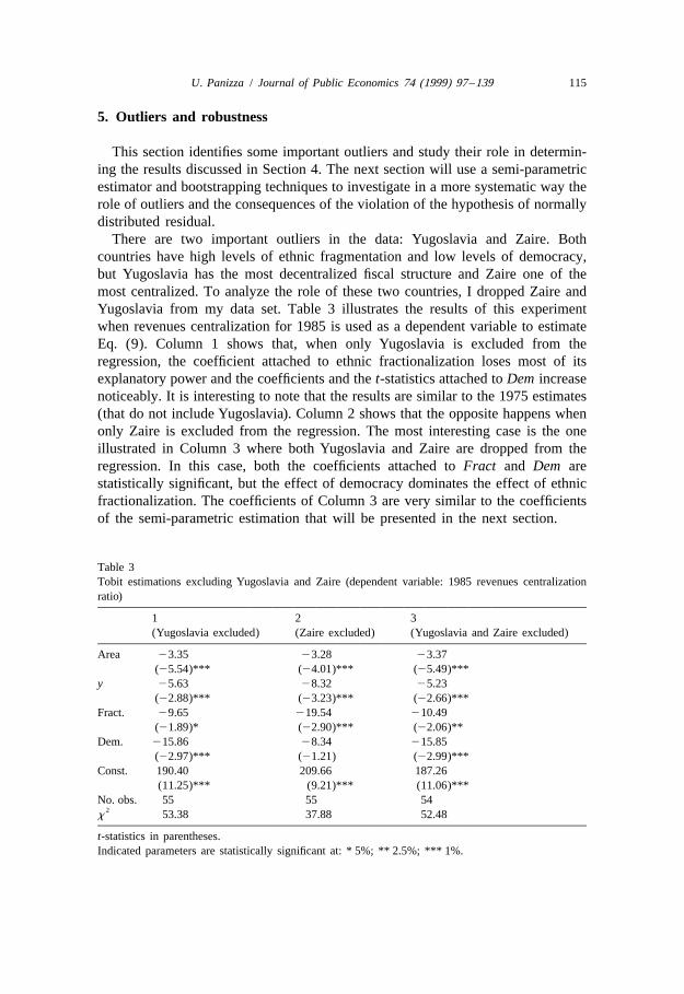
There are two important outliers in the data: Yugoslavia and Zaire. Bothcountries have high levels of ethnic fragmentation and low levels of democracy,but Yugoslavia has the most decentralized fiscal structure and Zaire one of themost centralized. To analyze the role of these two countries, I dropped Zaire andYugoslavia from my data set. Table 3 illustrates the results of this experimentwhen revenues centralization for 1985 is used as a dependent variable to estimateEq. (9). Column 1 shows that, when only Yugoslavia is excluded from theregression, the coefficient attached to ethnic fractionalization loses most of itsexplanatory power and the coefficients and the t-statistics attached to Dem increasenoticeably. It is interesting to note that the results are similar to the 1975 estimates(that do not include Yugoslavia). Column 2 shows that the opposite happens whenonly Zaire is excluded from the regression. The most interesting case is the oneillustrated in Column 3 where both Yugoslavia and Zaire are dropped from theregression. In this case, both the coefficients attached to Fract and Dem arestatistically significant, but the effect of democracy dominates the effect of ethnicfractionalization. The coefficients of Column 3 are very similar to the coefficientsof the semi-parametric estimation that will be presented in the next section.
Table 3Tobit estimations excluding Yugoslavia and Zaire (dependent variable: 1985 revenues centralizationratio)
1 2 3(Yugoslavia excluded) (Zaire excluded) (Yugoslavia and Zaire excluded)
Area 23.35 23.28 23.37(25.54)*** (24.01)*** (25.49)***
y 25.63 28.32 25.23(22.88)*** (23.23)*** (22.66)***
Fract. 29.65 219.54 210.49(21.89)* (22.90)*** (22.06)**
Dem. 215.86 28.34 215.85(22.97)*** (21.21) (22.99)***
Const. 190.40 209.66 187.26(11.25)*** (9.21)*** (11.06)***
No. obs. 55 55 542
x 53.38 37.88 52.48
t-statistics in parentheses.Indicated parameters are statistically significant at: * 5%; ** 2.5%; *** 1%.
116 U. Panizza / Journal of Public Economics 74 (1999) 97 –139
Economists and statisticians do not agree on the way one should treat outliers.Some think that outliers distort the estimations and they should be excluded fromthe model. Others claim that outliers provide interesting information. Paradoxical-ly, Yugoslavia and Zaire seem to be good real-world examples of the situationdescribed in the model of Section 2. In both countries, we observe two opposingforces: low levels of democracy that tend to make the country more centralizedand highly ethnically fractionalized populations that push for more decentraliza-tion. The outcome probably depends on the cost of repression (a very repressivecentral government may face international sanctions). It is reasonable to think thatthe latter will depend on the ‘visibility’ of a country. So, high levels of repressionmay have been very costly for a country like Yugoslavia (located at the center ofEurope), while the costs of repression may have been lower in Zaire.
The recent history indicates that both democracy and ethnic fractionalizationplayed an important role in Yugoslavia. This country was kept unified and fairlystable by a powerful and charismatic leader: Marshall Josip Tito. Tito’s death wassoon followed by the break-up of Yugoslavia.
As pointed out in Section 3.1, the values for fiscal centralization in Yugoslaviaare suspiciously low and might not reflect the true division of powers betweencentral and local governments. In this case, Yugoslavia would not be a true outlier,but only an observation not accurately measured. Since Yugoslavia has such animportant weight in determining the role of ethnic fractionalization, it is interestingto do a sensitivity analysis and explore the effects of different values of itscentralization ratio. To this purpose, I re-estimated the equation for revenuecentralization in 1985 using different values for Yugoslavia. When revenues
18centralization for Yugoslavia is between 0.5 and 0.85, both ethnic fractionaliza-tion and democracy are statistically significant.
While Area, GDP per capita, and ethnic fractionalization are very likely to beexogenous with respect to fiscal centralization, reverse causation from centraliza-tion to democracy may be a problem. The promotion and preservation ofdemocracy was one of the main reasons why the American founding fathers chosea highly decentralized system. De Tocqueville in La Democratie en Ameriquepraises the highly decentralized American system and claims that such a system isthe best protection for democracy. Although the events of the recent years (Spain,Czechoslovakia, Poland and the Soviet Union) seem to indicate a clear causationfrom democracy to decentralization, it is interesting to explore the reversecausation issue by using an instrument for the democracy variable. The problem is,as usual, the identification of a good instrument. An attempt was made by usingthe lagged value of democracy. This variable is highly correlated with democracy
19and therefore has all the statistical characteristics to be a good instrument. The
18 These seem to be reasonable values given the fact that only two countries have centralizationratios lower than 0.5 (Yugoslavia and Canada).
19 However, even if the use of this variable rules out direct reverse causation, there may still exist asystematic relationship between democracy and centralization.

U. Panizza / Journal of Public Economics 74 (1999) 97 –139 117
instrumental variables estimates (available upon request) are almost identical to theresults of the Tobit estimations with no instruments.
5.1. Semi-parametric estimations
Similarly to OLS, the Tobit model yields consistent parameter estimates if theresiduals are homoskedastic and normally distributed. While ordinary least squaresare very robust, and a violation of these hypotheses leads to inefficient but stillconsistent estimates, this is not the case for the Tobit model. Maximum likelihoodmethods can only be used to estimate censored regression models if thedistribution of the residuals is known. Greene (1993) discusses the consequencesof a mis-specification of the distribution of the residuals and shows that theviolation of the normality and homoskedasticity hypotheses leads to inconsistentestimates of the parameters.
In recent years many semi-parametric estimators that do not require anyassumption on the distribution of the residuals have been proposed. The symmetri-cally trimmed least squares estimator (STLS) and the censored least absolutedeviation estimator (CLAD) proposed by Powell (1984), (1986) do not requirei.i.d. errors but they do not perform well in small samples. The pairwise difference
´estimator (PD) proposed by Honore and Powell (1994) requires i.i.d. residuals butperforms relatively well in small samples. Monte Carlo simulations have shownthat, with a sample size of 50 observations, the PD estimator is often close to thebest estimator.
Since the data set used in this paper contains less than 70 observations, I´decided to use Honore and Powell’s PD to estimate Eq. (9). (Appendix F contains
´a description of the Honore and Powell pairwise difference estimator.) Table 4presents the results obtained by using this estimator. The number in parenthesesindicate the probability of a sign switch. These pseudo p-values were obtained bybootstrapping the model 1000 times.
The semi-parametric estimations of the coefficients of Area and y are similar tothe ones obtained in the OLS and Tobit estimations. The semi-parametricestimator instead produces very different results for the coefficients attached toethnic fractionalization and democracy. The coefficients attached to Fract arealways lower than the Tobit estimates and the coefficients attached to Dem alwayshigher. Ethnic fractionalization is statistically significant at the 5% level when thedependent variable is revenues in 1985 and statistically significant at the 10% levelwhen the dependent variable is revenues in 1980. In the expenditure regressions,the coefficient attached to ethnic fractionalization is statistically significant (with ap-value of 0.051) only in 1980. Democracy enters in the regression with astatistically significant coefficient for both expenditure and revenues in 1975 andfor revenues in 1985.
The results of the semi-parametric estimations are much closer (in themagnitude of both the parameters and their p-values) to the results of Column 3 ofTable 3 than to the Tobit results for the whole sample. In the Tobit estimations for

118 U. Panizza / Journal of Public Economics 74 (1999) 97 –139
Table 4Semi-parametric estimations
Revenues centralization ratios
1975 1980 1985
Area 23.33 22.82 23.53(0.000) (0.002) (0.000)
y 24.18 26.68 26.27(0.026) (0.002) (0.002)
Fract. 24.47 28.45 210.19(0.275) (0.095) (0.044)
Dem. 212.64 25.46 212.46(0.025) (0.19) (0.030)
Const. 170.8 182.38 193.42(0.000) (0.000) (0.000)
No. obs. 57 56 56Expenditure centralization ratios
1975 1980 1985
Area 22.99 23.04 23.25(0.002) (0.002) (0.002)
y 23.98 26.03 26.92(0.082) (0.001) (0.001)
Fract. 0.05 210.45 25.71(0.492) (0.051) (0.200)
Dem. 213.54 26.78 26.05(0.007) (0.189) (0.240)
Const. 163.96 182.49 190.17(20.000) (0.000) (0.000)
No. obs. 55 56 54
Pseudo p-values in parentheses.
the whole sample, Fract has a coefficient of 218.43 (and a t-statistic of 2.73),which is 80% higher (in absolute value) than the coefficient obtained with the PDestimator (210.19). At the same time, the coefficient of the Tobit estimation thatexcludes Yugoslavia and Zaire is almost identical to the coefficient of the PD
´estimation for the whole sample. This is an indication that the Honore and Powellmethod and the bootstrapping downweigh outliers and implicitly correct for someof the problems in the data. To conclude, the PD estimator reduces the explanatorypower of ethnic fractionalization and increases the explanatory power of thedemocracy variable, but still finds a negative correlation between these twovariables and the level of fiscal centralization.
After exploring the existence of a statistically significant relationship betweencentralization and a set of socio-economic variables, it is worth asking if thisrelationship is also economically significant. The results of Table 4 indicate that,for the 1985 sample, a 1 standard deviation increase in ethnic fractionalization is
U. Panizza / Journal of Public Economics 74 (1999) 97 –139 119
associated to a 2.8% decrease in revenues centralization. At the same time, a 1standard deviation increase of democracy in 1985 is associated to a 4.3% decreasein centralization. The effects on centralization associated to changes in income percapita and area size are also very large (ranging from 0.5 to 6%). This allows toconclude that the relationship between centralization and the set of socio-economicvariables used in this paper is not only statistically significant but also econ-omically significant.
6. The role of history
History is the main reason why many scholars claim that it is not possible to useeconomic theory to explain cross-country differences in the division of powersamong different levels of government. Many political scientists have pointed outthat, in each country, intergovernmental fiscal relations are the outcome of abargaining process that is generally unpredictable (Oates, 1972). In some cases,this bargaining process generated a structure of intergovernmental fiscal relationsthat, although optimal at the time the process took place, may not reflect thecurrent preferences of the citizens. In other cases, the level of fiscal centralizationmay have been imposed by a dictator (or monarch) or by international pressurewithout any consideration for the citizens’ preferences. Since the process ofadjusting to the optimal fiscal structure requires time, many countries may still befar away from their optimal level of centralization.
Although the model presented in Section 2 is static, it is interesting to study ifsome of the countries included in the sample are out of the equilibrium and slowlyadjusting towards it. An ideal way to control for the role of history would be toinclude in the regression fiscal centralization measured at the time a given country
20achieved its independence, but this variable is not available. An alternativemethod is to augment the regression with the lagged value of fiscal centralization.
20 Attempts to find proxies for the distance from the optimal fiscal structure were not successful. Tothis purpose I explored variables like social unrest, presence of independentist movement, or number ofyears since a given country has started its adjustment process. All these variables present conceptualproblems. The first set of variables (social unrest and presence of independentist movement) is likely tobe the effect and not the cause of a sub-optimal fiscal structure. The latter variable has the advantage ofbeing exogenous but it is not easily measurable. The problem with this variable is to identify a startingpoint. While this is not very difficult for countries like the UK or the US that have had a very stablepolitical system and the same form of government for more than two centuries, other countries posevery serious problems. How does one deal with cases like France, where there have been severalchanges in the constitution in the last 40 years? Or Spain? Should one start counting after the death ofFranco? What about Italy where there is a large consensus for a more decentralized system but nothinghas changed so far? Exogenous shocks, like the end of the Cold War, seriously reshaped the politicalequilibrium in Europe and modified the status quo. Unfortunately, the available data stop in 1985 and itis impossible to control for these events.

120 U. Panizza / Journal of Public Economics 74 (1999) 97 –139
To this purpose, I included fiscal centralization in 1975 among the explanatory21variables for fiscal centralization in 1985.
The results (reported in Table 5) confirm the fact that history is very important.The lagged value of fiscal centralization absorbs most of the variance of theregression (but its coefficient is significantly lower than 1) and reduces theexplanatory power of the other variables. Although the explanatory power of Areaand y decrease noticeably, the correlation between Fract and fiscal centralizationis robust to the inclusion of the lagged dependent variable. It is not surprising thatfiscal centralization is highly correlated with its lagged value. Most of theexplanatory variables are either almost constant (like ethnic fractionalization andarea) or highly correlated (like GDP and democracy) over time. The fact that, evenwhen the lagged value is included, the other explanatory variables still have somepower in explaining fiscal centralization suggests the idea that, while somecountries have reached their equilibrium level of fiscal centralization, others arestill adjusting towards it.
The very recent history shows that for some countries even the overall borderswere not optimal from the point of view of their citizens. It is not surprising thatthe borders of these countries had not been fixed by a national movement butimposed by outside forces (this is the case for the separation of West and EastGermany) or were the output of a highly non-democratic process (Yugoslavia andCzechoslovakia, for instance). The borders of other countries, especially in Africa,
Table 5Tobit estimations (dependent variables: 1985 revenues and expenditure centralization ratios)
Revenues centralization Expenditure centralization
Area 20.82 20.89(22.19)** (22.00)*
y 21.32 23.27(21.20) (22.19)**
Fract. 25.93 27.91(22.08)** (22.26)**
Dem. 23.50 21.64(21.25) (20.44)
Centr. 1975 0.87 0.80(16.48)*** (12.19)***
Const. 37.54 60.95(2.80)*** (3.66)***
No. obs. 53 512
x 125.37 93.90
t-statistics in parentheses.Indicated parameters are statistically significant at: * 5%; ** 2.5%; *** 1%.
21 When the 1975 values were missing, the 1980 values were used as proxy.
U. Panizza / Journal of Public Economics 74 (1999) 97 –139 121
were determined by their former colonial authorities. Even countries with a strongand long democratic history can be far away from the equilibrium level ofcentralization. The regression therefore pools together countries that may be veryclose to their optimal fiscal structure with countries that are far away from theoptimum and are slowly adjusting to it.
If we accept the idea that some countries are out of the equilibrium, theresiduals of the regression should be correlated with changes in fiscal centraliza-tion over time. Countries where the actual level of centralization is higher than thepredicted value (i.e., u .0) should be moving towards a more decentralizedi
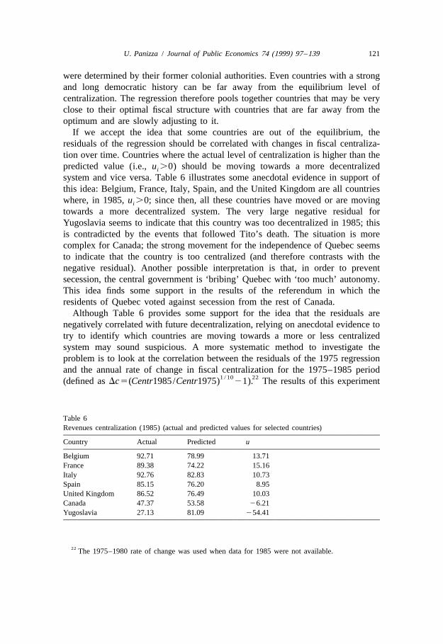
system and vice versa. Table 6 illustrates some anecdotal evidence in support ofthis idea: Belgium, France, Italy, Spain, and the United Kingdom are all countrieswhere, in 1985, u .0; since then, all these countries have moved or are movingi
towards a more decentralized system. The very large negative residual forYugoslavia seems to indicate that this country was too decentralized in 1985; thisis contradicted by the events that followed Tito’s death. The situation is morecomplex for Canada; the strong movement for the independence of Quebec seemsto indicate that the country is too centralized (and therefore contrasts with thenegative residual). Another possible interpretation is that, in order to preventsecession, the central government is ‘bribing’ Quebec with ‘too much’ autonomy.This idea finds some support in the results of the referendum in which theresidents of Quebec voted against secession from the rest of Canada.
Although Table 6 provides some support for the idea that the residuals arenegatively correlated with future decentralization, relying on anecdotal evidence totry to identify which countries are moving towards a more or less centralizedsystem may sound suspicious. A more systematic method to investigate theproblem is to look at the correlation between the residuals of the 1975 regressionand the annual rate of change in fiscal centralization for the 1975–1985 period
1 / 10 22(defined as Dc5(Centr1985/Centr1975) 21). The results of this experiment
Table 6Revenues centralization (1985) (actual and predicted values for selected countries)
Country Actual Predicted u
Belgium 92.71 78.99 13.71France 89.38 74.22 15.16Italy 92.76 82.83 10.73Spain 85.15 76.20 8.95United Kingdom 86.52 76.49 10.03Canada 47.37 53.58 26.21Yugoslavia 27.13 81.09 254.41
22 The 1975–1980 rate of change was used when data for 1985 were not available.

122 U. Panizza / Journal of Public Economics 74 (1999) 97 –139
Table 7Correlation between the residuals for the 1975 regression and rate of change in fiscal centralization inthe following decade
Revenues centralization Expenditure centralization
Correlation 20.40 20.51p value 0.0045 0.0003No. obs. 48 45
strongly support the idea that the 1975 residuals are negatively correlated with thesubsequent changes in fiscal centralization. Table 7 provides evidence for the factthat countries that are out of the equilibrium are slowly moving towards it and thatEq. (9) is a good specification to analyze the empirical determinants of fiscalcentralization.
Some evidence that countries are adjusting toward an equilibrium can also befound in the fact that the 1985 equation fits the data much better than the 1975
2¯equation. When an OLS regression is performed on the same set of countries Rincreases from 0.47 to 0.56. At the same time the sum of squared errors of theTobit regression decreases from 4670 to 3842.
One should be careful in interpreting the results of this section. In particular,they do not provide any additional support for the model of Section 2. The latter isset in a purely static framework, while the issues discussed in this section aredynamic. In fact, this section shows that there are changes in the level ofcentralization that cannot be explained by the set of regressors used in this paper,and calls for further research on the transitional dynamics of the decentralizationprocess.
7. Conclusions
In the real world, democratization has often been followed by decentralization.This happened in Spain, where the death of Francisco Franco and the return to ademocratic system was soon followed by a massive process of decentralization.Other examples are Poland, Czechoslovakia, Russia and the Ukraine. The end ofthe Cold War also favored the rise of secessionist (or pro-decentralization) politicalmovements in countries that, although democratic, used to have an extremely rigidpolitical situation. In Italy, for instance, the end of the ‘Cold War equilibrium’ wassoon followed by the rise of a separatist political party. The model and empiricalanalysis presented in this paper try to shed some light on these recent events.
Many authors think that it is not possible to find a single set of variablesexplaining the cross-country differences in the degree of fiscal centralization.

U. Panizza / Journal of Public Economics 74 (1999) 97 –139 123
Oates (1972) attempt seems to support this view. This paper is more optimist onthe possibility of finding empirical regularities explaining decentralization. I findthat country size, income per capita, ethnic fractionalization, and the level ofdemocracy are negatively correlated with fiscal centralization.
The main problem with the results described above is their sensitivity to outliersand to the use of different samples. While Area and GDP per capita are robustlycorrelated with centralization in almost all specifications, ethnic fractionalizationand democracy have unstable coefficients, highly dependent on the sample used.This is due to the fact that outliers play a very important role in determining thesecoefficients. Yugoslavia is a particularly troublesome outlier. Its very low level offiscal centralization plays an enormous weight in determining the coefficients (andt-statistics) attached to democracy and ethnic fractionalization. When Yugoslavia isdropped from the sample, democracy becomes strongly correlated with decentrali-zation. This is also true when more realistic values are used for fiscal centralizationin Yugoslavia.
To conclude, this paper shows that there are some regularities that can be usedto explain the cross-country variations in the degree of fiscal centralization. Inparticular, if one believes that outliers are important and that they should not beeliminated from the analysis, then it is possible to conclude that land area, GDPper capita, and ethnic fractionalization are associated with fiscal decentralization.If, however, one believes that outliers should be eliminated, the analysis shows astrong correlation between fiscal centralization and each of land area, GDP percapita, and Democracy.
This paper indicates that there are open avenues for further research both on theempirical and theoretical sides. On the empirical side, it would be interesting toidentify a homogeneous definition of jurisdiction and augment Eq. (9) with avariable measuring the number of jurisdictions. On the theoretical side there aremany possible extensions. The first relates to extending the results to a case of acircular country and relaxing the assumption of perfect sorting of the citizens. Itwould be interesting to show whether the results of this paper are robust to a casewhere preferences are highly, but not perfectly, correlated with location.
Introducing income heterogeneity would be another interesting extension.Section 2 shows that the equilibrium level centralization is decreasing in income.Therefore, a model where individuals are sorted according to their income shouldpredict that the policies of the central government are closer to the preferences ofthe rich. This could be used to explain the fact that upper classes tend to havehigher political participation and influence than poorer classes.
The results of Section 6 seem to indicate that the adjustment toward the optimalfiscal structure takes time. This cannot be captured by the static model of Section2. It would then be an interesting exercise to extend the model to a dynamicframework and try to obtain some information on why some countries reached theequilibrium faster than others or explain the overshooting that characterized othercountries (for instance Poland).

124 U. Panizza / Journal of Public Economics 74 (1999) 97 –139
Acknowledgements
This paper, based on the second chapter of my Ph.D. dissertation at the JohnsHopkins University, was written while I was at the Department of Economics ofthe University of Turin. I would like to thank Nada Choueiri, Ernesto Stein, twoanonymous referees, seminar participants at the JHU, University of Adelaide,University of South Florida, Inter-American Development Bank, University ofCagliari, and University of Turin for helpful comments. I am also grateful toLaurence Ball and Louis Maccini for useful comments and constant support, and
´Marisa Apa Domino for suggesting the use of the Honore and Powell estimatorand sharing her program with me. The usual caveats apply. The opinionsexpressed in this paper are my own and do not necessarily reflect the views of theInter-American Development Bank.
Appendix A
Proof of Proposition 1
We want to show that g*5(my /(m 1b )) (with m 512a[u(S /4)1(12u )(S /4J)]) is the amount of public good preferred by the median voter. This isequivalent to showing that half of the population would like to consume an amountof g larger than g* and the other half of the population would like to consume andamount of g smaller than g*.
In Eq. (1) it was shown that g 5(d y) /(d 1b ), with d 512a(ul 1(12u )l ).i i i i im ij
Note that, since we assume a continuum of individuals, for half of the populationl ,(S /4) and for the other half l .(S /4). Also, for half of the populationim im
l ,(S /4J) and for the other half l .(S /4J). Therefore, when u 51 or u 50,ij ij
Proposition 1 is trivially true.2Since (≠g /≠d )5(by /(d 1b ) ).0, individuals with larger d (and thereforei i i
smaller l and l ) prefer a larger amount of public good. It is therefore possible toim ij
divide the population into four groups as shown in Fig. 2. For a fraction F of
Fig. 2. Preferences for the size of the public good.
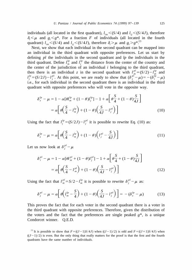
U. Panizza / Journal of Public Economics 74 (1999) 97 –139 125
individuals (all located in the first quadrant), l ,(S /4) and l ,(S /4J), thereforeim ij
d ,m and g ,g*. For a fraction F of individuals (all located in the fourthi i23quadrant) l ,(S /4) and l ,(S /4J), therefore d .m and g .g*.im ij i i
Next, we show that each individual in the second quadrant can be mapped intoan individual in the third quadrant with opposite preferences. Let us start bydefining pl the individuals in the second quadrant and lp the individuals in the
lp lpthird quadrant. Define l and l the distance from the center of the country andm j
the center of the jurisdiction of an individual i belonging to the third quadrant,pl lpthen there is an individual z in the second quadrant with l 5(S /2)2l andm m
lp pl pl lpl 5(S /2J)2l . At this point, we are ready to show that (d 2m)52(d 2m)j j z i
i.e., for each individual in the second quadrant there is an individual in the thirdquadrant with opposite preferences who will vote in the opposite way.
S Slp lp lp ] ]F Gd 2 m 5 1 2 a[ul 1 (1 2u )l ] 2 1 1 a u 1 (1 2u )z m j 4 4J
S Slp pl] ]F S D S DG5 a u 2 l 1 (1 2u ) 2 l (10)m j4 4J
lp plUsing the fact that l 5(S /2J)2l it is possible to rewrite Eq. (10) as:j j
S Slp lp pl] ]F S D S DGd 2 m 5 a u 2 l 1 (1 2u ) l 2 (11)z m j4 4J
plLet us now look at d 2mj
S Spl pl pl ] ]F Gd 2 m 5 1 2 a[ul 1 (1 2u )l ] 2 1 1 a u 1 (1 2u )i m j 4 4J
S Spl pl] ]F S D S DG5 a u 2 l 1 (1 2u ) 2 l (12)m j4 4J
pl lp plUsing the fact that l 5S /22l it is possible to rewrite d 2m as:m m j
S Spl lp pl lp] ]F S D S DGd 2 m 5 a u l 2 1 (1 2u ) 2 l 5 2 (d 2 m) (13)j m j z4 4J
This proves the fact that for each voter in the second quadrant there is a voter inthe third quadrant with opposite preferences. Therefore, given the distribution ofthe voters and the fact that the preferences are single peaked g*, is a uniqueCondorcet winner. Q.E.D.
23 It is possible to show that F5((J21)S /4J) when ((J21) /2) is odd and F5((J11)S /4J) when((J21) /2) is even. But the only thing that really matters for the proof is that the first and the fourthquadrants have the same number of individuals.

126 U. Panizza / Journal of Public Economics 74 (1999) 97 –139
Appendix B
Proof of Proposition 2
The proof of this proposition requires some simple, but long and tedious,algebra. I start by establishing some basic results:
aS(J 2 1)]]]m 5 2 , 0; m 5 0;u uu4J
S S 2 S(J 2 1)] ] ]]]]F Gm 5 2 u 1 (1 2u ) , 0; m 5 m 5 , 0;a au ua4 4J 4J
1 1 2 a(J 2 1)] ] ]]]]F Gm 5 2 a u 1 (1 2u ) , 0; m 5 m 5 , 0;S uS Su4 4J 4J
a(1 2u )S 2 aS]]] ]]m 5 . 0; m 5 m 5 , 0;J 2 Ju uJ 24J 4J
2bym 2 2by(m )≠g ≠c u u
] ] ]]] ]]]]5 2 5 , 0; g 5 , 0;2 uu 3≠u ≠u (b 1 m) (b 1 m)
bym m (b 1 m) 2 2m m≠g ≠c a au a u] ] ]]] ]]]]]]5 2 5 , 0; g 5 g 5 by , 0;2 ua au 3≠a ≠a (b 1 m) (b 1 m)
bym m (b 1 m) 2 2m m≠g ≠c S Su S u] ] ]]] ]]]]]]5 2 5 , 0; g 5 g 5 by , 0;2 uS Su 3≠S ≠S (b 1 m) (b 1 m)
bym m (b 1 m) 2 2m m≠g ≠c ,J Ju J u] ] ]]] ]]]]]]5 2 5 , 0; g 5 g 5 by 502 uJ Ju 3≠J ≠J .(b 1 m) (b 1 m)
Using the fact that (≠g /≠u )52(≠c /≠u ), it is possible to write the government’sF.O.C. as:
≠V 1 2 fgov med med]] ]]5 fg U 2 U 1 u 1 (1 2 f)g 5 0 (14)S Du g c≠u f
For the median voter of the central jurisdiction (and therefore the government),med medU 2U 5U ((1 /g)2(b /c))5(U (b 1m) /y)((12m) /m),0 (because m ,1).g c
Therefore the first term of Eq. (14) is negative and the second is positive. Byderiving implicitly Eq. (14), it is possible to study the effect of the exogenousvariables on the level of fiscal centralization.
U. Panizza / Journal of Public Economics 74 (1999) 97 –139 127
1 2 fmed med ]]V 5 fg U 2 U 1 uS Duu uu g c f
1 2 fmed med med ]]1 fg g (U 1 U 2 2U ) 1 1 (1 2 f)g (15)S Du u gg cc cg uf
med med medSince g ,0 and (U 1U 22U ),0, V ,0. This result, besides beinguu gg cc cg uu
necessary to compute the effect of the independent variables on the level ofcentralization, also shows that the government’s utility function is concave andtherefore the F.O.C. of Eq. (14) is necessary and sufficient for a maximum.
1 2 fmed med med med med]]V 5 fg U 2 U 1 u 1 fg ( g (U 1 U 2 2U ))S Dua ua g c u a gg cc cgf
1 (1 2 f)g , 0 (16)a
1 2 fmed med med med med]]V 5 fg U 2 U 1 u 1 fg ( g (U 1 U 2 2U ))S DuS uS g c u S gg cc cgf
1 (1 2 f)g , 0 (17)S
med medV 5 g (U 2 U ) 2 ( g u 1 g) , 0 (18)uf u g c u
Note that V ,0 because Eq. (14) requires that ( g u 1g).0.uf u
1 2 fmed med med med med]]V 5 fg U 2 U 1 u 1 fg ( g (U 1 U 2 2U ))S DuJ uJ g c u J gg cc cgf
,
1 (1 2 f)g 50 (19)J.
To investigate the role of a change in income let us start by noting thatg 5g(bm /m(m 1b )), therefore Eq. (14) can be rewritten as:u u
≠Vgov]] 5 g (1 2 f)F
≠u
medbm 1 2 f U (b 1 m) 1u]]] ]] ]]]] ]1 f u 1 2 1 5 0 (20)S DGS Df y mm(m 1 b )
Since g50 is a minimum, it must be true that
medbm U (b 1 m) 1 2 mu]]] ]]]]]](1 2 f) 1 f u 1 5 0.S DF Gy mm(m 1 b )
It is now possible to show that:
2b med]V 5 fm (1 2 m) gU , 0S Duy u my

128 U. Panizza / Journal of Public Economics 74 (1999) 97 –139
Therefore:
V VV V≠u ≠u ≠u ≠uuf uyua uS] ] ] ] ] ] ] ]5 2 , 0; 5 2 , 0; 5 2 , 0, 5 2≠a V ≠S V ≠f V ≠y Vuu uu uu uu
V≠u ,uJ] ], 0, and 5 2 50≠J V .uu
A corollary to Proposition 3 is that f 51 will lead the central government to setu 50. This is easily shown by observing that, when f 51, Eq. (14) becomes
med med(≠V /≠u )5g (U 2U ),0. Q.E.D.gov u g c
To prove that a Benthamite social planner will set u 50 it is sufficient to showthat the social planner’s utility function is strictly decreasing in u. Let us start bywriting the social planner’s problem:
N N
sp d bimax U 5E U di 5E g c di (21)iu
0 0
N Nsp ≠d g≠U i u
]] ] ]5 ln( g) E U di 1 E U [d 2 m]di (22)i i i≠u ≠u g0 0
N
Now note that the ln ( g)e U (≠d /≠u ) di , 0 (because g.1). Proposition 1 showsi i0
that m is the median (and, given the assumption of uniform distribution ofN
individuals, also the mean) value of d . Therefore e [d 2 m]di 5 0, but since in-i i0
dividuals for which d .m have levels of utility higher than those of individuals foriN
which d ,m, then e U [d 2 m]di . 0, the second term of Eq. (22) will then be nega-i i i0
sptive and (≠U /≠u ),0. Q.E.D.
Appendix C
Data sources
This appendix describes the source of the data used.

U. Panizza / Journal of Public Economics 74 (1999) 97 –139 129
Table 8Centralization ratios
Revenues Expenditure
1975 1980 1985 1975 1980 1985
Argentina 76.21 60.86 84.36 70.46 72.72 74.50Australia 78.62 79.29 76.96 85.04 79.01 78.00Austria 72.81 74.71 72.37 73.48 75.66 75.25Barbados 100.00 99.96 100.00 100.00 100.00 100.00Belgium 94.68 92.70 91.75 95.03Bolivia 86.28 95.82Brazil 71.27 79.18 78.20 69.08 77.49 70.59Canada 53.18 47.42 47.37 53.97 50.55 52.16Cent. Afr. Rep. 100.00Chile 98.24 97.53 94.25 96.96 96.28 94.89Colombia 85.00 82.68 80.03 90.01 83.55 81.90Congo 79.77Costa Rica 96.93 95.80 96.46 96.38 97.75 97.47Cyprus 97.43 98.53Denmark 66.60 67.76 69.77 56.62 69.30 71.03Dominican Rep. 98.02 98.29 98.49 98.45 98.84Egypt 100.00 100.00 100.00 100.00 100.00Ethiopia 97.71 97.52 98.56Finland 70.26 69.97 69.35 73.07 72.11 70.80France 89.82 90.32 89.38 88.11 90.71 89.96Gambia 93.29 94.60 93.54 97.33Germany 62.20 62.94 63.95 62.12 61.85 63.88Greece 97.38 97.43Guatemala 95.57 96.00Honduras 93.76 95.69Hungary 87.87 87.58 87.95 86.90Iceland 79.79 74.83 74.06 81.61 76.08India 67.34 73.79 70.36 74.26 73.69 77.94Indonesia 96.55 97.63 97.45 97.23 98.58 98.95Iran 98.49 91.70 95.16 98.69 97.47 95.72Iraq 74.92Ireland 85.18 92.22 93.26 87.73 95.54 96.84Israel 95.51 94.66 95.59 96.70 95.52Italy 94.65 92.76 91.11 77.31Jordan 92.00 94.35Kenya 91.41 93.74 94.33 98.88 95.45 96.35Korea 85.54 89.38Kuwait 94.23 100.00 100.00 100.00Lesotho 100.00 100.00 100.00Luxembourg 91.73 81.71 99.82 88.96 90.14 86.88Malawi 94.11 94.33 96.51 94.45Malaysia 90.43 84.67 86.48 84.11 85.85 86.51Malta 100.00 100.00 100.00 99.98 100.00 100.00Mauritius 91.29 92.23 99.08Mexico 81.57 80.35 82.77 82.51 81.41 87.52

130 U. Panizza / Journal of Public Economics 74 (1999) 97 –139
Table 8. Continued
Revenues Expenditure
1975 1980 1985 1975 1980 1985
Myanmar 100.00 100.00 66.66 100.00 100.00Netherlands 97.14 95.63 95.90 96.67 94.91 95.79New Zealand 88.80 89.61Norway 66.95 82.13 83.11 69.16 79.40 82.16Pakistan 72.75 83.75 78.82Panama 96.35 97.69 97.68 97.20 98.20 98.09Paraguay 96.78 95.51 95.57 96.86 95.14 95.01Peru 84.28 87.37 86.15Poland 89.56 91.26Portugal 96.48 92.57Romania 88.73 90.14 91.03 90.85 90.55Senegal 83.43Singapore 100.00 100.00 100.00 100.00 100.00 100.00South Africa 82.20 85.45 84.66 86.28Spain 95.09 88.87 85.16 94.20 90.37 87.37Sri Lanka 94.31 96.51 94.54 96.48 98.26 97.70Sudan 93.13Sweden 71.24 69.31 73.17 69.61 74.02 74.33Switzerland 52.15 53.25 53.28 53.81 55.46 47.94Thailand 92.87 91.61 94.14 94.44 96.40 96.05Trinidad 99.76Tunisia 97.42 96.88United Kingdom 84.41 86.86 86.53 84.44 85.99 89.93United States 60.43 63.35 60.11 65.36 68.18 68.63Uruguay 89.68 90.93 90.50 92.52 91.59 92.50Venezuela 99.28 98.55Yemen 100.00 100.00 100.00 100.00Yugoslavia 29.17 27.14 29.62 28.36Zaire 100.00 100.00 100.00 100.00 100.00Zimbabwe 72.75 77.64 82.05 81.87 85.10No. obs. 57.00 56.00 56.00 55.00 55.00 54.00Mean 87.31 85.49 86.19 86.96 86.90 85.84S.D. 13.15 15.12 14.88 13.21 14.49 14.74
1. Data on fiscal centralization. The data on fiscal centralization were computedas the percentage of central government revenues (expenditure) on the total(central plus local) government revenues (expenditure). The data on central andtotal government (general government, in the IMF terminology) revenues andexpenditures were obtained from the IMF (1975, 1980 and 1985) GovernmentFinance Statistics Yearbook. When the full set of data was not available for theyears considered in this study (i.e., 1975, 1980 and 1985) but it was available
U. Panizza / Journal of Public Economics 74 (1999) 97 –139 131
for the previous or following year the available data were used. The data for1975 were not available for Zimbabwe and Sudan (1976 was used instead of1975). The data for 1980 were not available for the Central African Republic,Hungary, Pakistan, Venezuela and Egypt. For the first two countries 1981 datawere used and for the last three countries 1979 data were used. Data for 1984instead of 1985 were used for Bolivia, Colombia, Kenya, Malawi, Switzerlandand Uruguay.
2. Data on ethnic fractionalization. The data on ethnic fractionalization,originally published in the Atlas Narodov Mira, were obtained from Taylor andHudson (1972).
3. Data on democracy. The data on democracy are from Gastil (1990); Barro(1996). The data were available for 1975, 1978 and 1988 only. The 1978 datawere used to measure democracy in 1980 and the average between 1978 and1988 was used to measure democracy in 1985.
4. Data on area and population. World Development Indicator (World Bank,1990).
5. Data on GDP. The data on GDP are from Summers and Heston (1991).
Appendix D
OLS estimations
Given the fact that the dependent variable is censored at 100, OLS is not theappropriate technique to estimate the equations described in Section 4. Thisappendix presents the results of least squares regressions in order to compare themwith Oates (1972) results.
The OLS estimates are presented in Table 9. When the dependent variable istotal revenue, Area and GDP per capita have negative and statistically significant
24coefficients. Fract has always a negative coefficient, not statistically significantfor 1975 and statistically significant at 2.5% and 1% level for 1980 and 1985.Democracy seems to play an important role in explaining fiscal centralization in1975, but this effect disappears in 1980 and 1985.
The expenditure regressions do not fit the data as well as the revenueregressions, but the results of the two sets of regressions are similar. As for therevenue regressions, Democracy has an important weight in explaining centraliza-
24 I tried to introduce the square of GDP per capita to control for non-linearities, but its coefficientturned out not to be statistically significant.

132 U. Panizza / Journal of Public Economics 74 (1999) 97 –139
Table 9Least squares estimates
Revenues centralization ratios
1975 1980 1985
Area 22.51 22.177 22.474(24.082)*** (22.800)*** (23.532)***
y 23.723 28.834 27.643(21.868)* (23.633)*** (23.326)***
Fract. 25.480 214.982 214.613(20.994) (22.054)** (22.409)***
Dem. 211.947 20.087 24.862(22.592)*** (20.014) (20.774)
Const. 157.066 191.66 188.645(9.980)*** (8.964)*** (9.488)***
No. obs. 56 56 562R̄ 0.40 0.31 0.39
F 13.32 12.05 19.32Expenditure centralization ratios
1975 1980 1985
Area 22.498 2.183 22.396(23.901)*** (23.016)*** (23.267)***
y 23.363 27.691 28.93(21.592) (23.549)*** (23.430)***
Fract. 20.850 213.853 2 10.993(20.147) (22.195)** (21.682)
Dem. 211.987 21.179 20.003(22.183)** (20.206) (0.000)
Const. 151.744 183.642 194.645(9.095)*** (9.531)*** (8.602)***
No. obs. 55 56 542R̄ 0.35 0.33 0.34
F 10.55 14.46 15.81
t-statistics in parentheses.Parameters indicated are statistically significant at: * 5%; ** 2.5%; *** 1%.
tion in 1975, but no importance in 1980 and 1985 (the coefficients attached todemocracy in 1980 and 1985 are higher in the revenues regressions). Fract isstatistically significant at the 2.5% level in the 1980 regression and statisticallysignificant at the 5% level in the 1985 regression.
Even if fundamentally flawed, the OLS analysis is instructive. Using the OLSestimate it is possible to compare the results of this paper with Oates (1972) andconclude that the differences are not only due to different estimation techniques,but also to the use of different data sets.
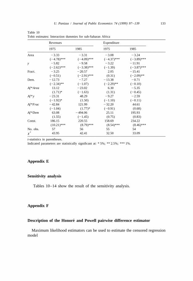
U. Panizza / Journal of Public Economics 74 (1999) 97 –139 133
Table 10Tobit estimates: Interaction dummies for sub-Saharan Africa
Revenues Expenditure
1975 1985 1975 1985
Area 23.33 23.31 23.08 23.24(24.78)*** (24.09)*** (24.37)*** (23.89)***
y 25.82 29.58 23.22 211.91(22.62)*** (23.38)*** (21.39) (23.87)***
Fract. 23.25 220.57 2.05 215.41(20.51) (22.91)*** (0.31) (22.09)**
Dem. 212.73 27.27 213.38 20.71(22.34)** (21.07) (22.29)** (20.10)
Af *Area 13.12 223.02 6.30 25.35(1.71)* (21.63) (1.31) (20.45)
Af *y 223.31 48.29 29.27 22.59(21.92)* (1.50) (21.10) (20.11)
Af *Frac 242.84 121.99 232.20 44.61(21.04) (1.77)* (20.91) (0.68)
Af *Dem 63.08 2494.06 25.11 195.93(1.55) (21.45) (0.75) (0.83)
Const. 186.15 220.55 158.69 234.22(10.21)*** (8.79)*** (8.54)*** (8.46)***
No. obs. 57 56 55 542
x 43.95 42.41 32.50 33.09
t-statistics in parentheses.Indicated parameters are statistically significant at: * 5%; ** 2.5%; *** 1%.
Appendix E
Sensitivity analysis
Tables 10–14 show the result of the sensitivity analysis.
Appendix F
´Description of the Honore and Powell pairwise difference estimator
Maximum likelihood estimators can be used to estimate the censored regressionmodel
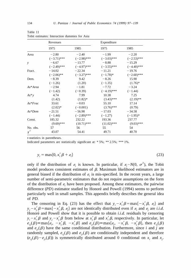
134 U. Panizza / Journal of Public Economics 74 (1999) 97 –139
Table 11Tobit estimates: Interaction dummies for Asia
Revenues Expenditure
1975 1985 1975 1985
Area 22.80 22.40 21.99 22.20(23.71)*** (22.98)*** (23.03)*** (22.53)***
y 26.67 213.77 28.88 215.29(22.49)*** (24.97)*** (23.55)*** (24.40)***
Fract. 214.02 222.34 211.21 219.76(22.06)** (23.27)*** (21.78)* (22.60)***
Dem. 28.39 9.42 28.26 15.90(21.26) (1.20) (21.35) (1.76)*
As*Area 22.94 21.81 27.72 23.24(21.42) (20.39) (24.19)*** (21.44)
As*y 4.74 7.99 10.38 7.25(1.42) (1.82)* (3.43)*** (2.19)**
As*Frac 33.61 20.03 55.10 17.14(2.02)* (20.001) (3.76)*** (0.79)
As*Dem 221.51 256.98 217.03 234.58(21.44) (22.89)*** (21.27) (21.95)*
Const. 185.32 232.22 193.36 237.77(9.69)*** (10.71)*** (11.02)*** (9.03)***
No. obs. 57 56 55 542
x 43.07 54.41 49.71 40.70
t-statistics in parentheses.Indicated parameters are statistically significant at: * 5%; ** 2.5%; *** 1%.
9y 5 maxh0, x b 1 ´ j (23)i i i
2only if the distribution of ´ is known. In particular, if ´ |N(0, s ), the Tobiti i
model produces consistent estimates of b. Maximum likelihood estimators are ingeneral biased if the distribution of ´ is mis-specified. In the recent years, a largei
number of semi-parametric estimators that do not require assumptions on the formof the distribution of ´ have been proposed. Among these estimators, the pairwisei
´difference (PD) estimator studied by Honore and Powell (1994) seems to performparticularly well in small samples. This appendix briefly describes the general ideaof PD.
9 9The censoring in Eq. (23) has the effect that y 2x b 5maxh2x b, ´ j andi i i i
9 9y 2x b 5maxh2x b, ´ j are not identically distributed even if ´ and ´ are i.i.d.j j j j i j
´Honore and Powell show that it is possible to obtain i.i.d. residuals by censoring9 9 9 9y 2x b and y 2x b from below at x b and x b, respectively. In particular, leti i j j j i
9 9 9 9e (b );maxh´ , 2x b, 2x bj and e (b );maxh´ , 2x b, 2x bj, then e (b )ij i j i ji j i j ij
and e (b ) have the same conditional distribution. Furthermore, since i and j areji
randomly sampled, e (b ) and e (b ) are conditionally independent and thereforeij ji
(e (b )2e (b )) is symmetrically distributed around 0 conditional on x and x .ij ji i j

U. Panizza / Journal of Public Economics 74 (1999) 97 –139 135
Table 12Tobit estimates: Sensitivity analysis using different definitions of size (1985)
Revenues (1985)
Area 23.97 23.97 2 3.97(23.33)*** (23.33)*** (23.33)***
Pop 1.34 1.31(0.84) (0.75)
Inc 1.35 0.00(0.85) (0.04)
y 28.74 210.09 28.77(23.42)*** (23.48)*** (23.31)***
Frac 219.38 219.38 219.39(22.84)*** (22.84)*** (22.84)***
Dem 28.83 28.83 28.87(21.28) (21.28) (21.27)
Const. 200.29 200.29 201.06(7.14)*** (7.14)*** (6.06)***
No. obs. 56 56 562
x 39.13 39.13 39.13Expenditure (1985)
Area 23.81 23.81 23.83(23.11)*** (23.11)*** (23.12)***
Pop 1.36 1.04(0.82) (0.58)
Inc 1.36 0.00(0.82) (0.44)
y 29.73 211.09 210.06(23.44)*** (23.51)*** (23.43)***
Frac 215.95 215.95 216.14(22.22)** (22.22)** (22.24)**
Dem 22.45 22.45 22.83(20.35) (20.35) (20.41)
Const. 201.30 201.30 209.39(6.37)*** (6.37)*** (5.90)***
No. obs. 54 54 542
x 30.67 30.67 30.87
t-statistics in parentheses.Indicated parameters are statistically significant at: * 5%; ** 2.5%; *** 1%.Area, Pop, Inc and y are in logs, except for the last column, where Inc is in levels.
´This allows Honore and Powell to use the moment condition of Eq. (24) to definean estimator for b.
E[j(e (b ) 2 e (b ))ux , x ] (24)ij ji i j
where j(?) is an odd function. Since it is not always easy to show that a set of

136 U. Panizza / Journal of Public Economics 74 (1999) 97 –139
Table 13Tobit estimates: Sensitivity analysis using different definitions of size (1975)
Revenues (1975)
Area 23.71 23.71 23.67(23.47)*** (23.47)*** (23.47)***
Pop 1.08 1.39(0.41) (1.02)
Inc 1.08 0.00(0.41) (0.67)
y 24.43 25.50 24.08(22.04)** (22.28)** (21.84)*
Frac 26.57 26.57 26.09(21.11) (21.11)*** (21.03)
Dem 213.38 213.38 213.00(22.41)** (22.41)** (22.35)**
Const. 162.37 162.37 154.30(7.72)*** (7.72)*** (6.41)***
No. obs. 57 57 572
x 38.26 38.26 38.70Expenditure (1975)
Area 22.89 22.89 22.88(22.66)*** (22.66)*** (22.70)***
Pop 20.50 0.03(20.04) (0.02)
Inc 20.50 0.00(20.04) (0.17)
y 23.35 23.30 23.25(21.52) (21.34) (21.43)
Frac 1.99 1.99 22.08(0.33) (0.33)** (20.34)
Dem 213.89 213.89 213.78(22.40)** (22.40)** (22.36)**
Const. 158.74 158.74 156.61(7.40)*** (7.40)*** (6.26)***
No. obs. 55 55 552
x 30.40 30.40 30.42
t-statistics in parentheses.Indicated parameters are statistically significant at: * 5%; ** 2.5%; *** 1%.Area, Pop, Inc and y are in logs, except for the last column, where Inc is in levels.
´moment conditions are satisfied at a given point, Honore and Powell define theestimator as the minimand of the following random function:
21nS DS (b) 5 O s( y , y , d ) (25)n i j2i,j
where d 5(x 2x )9b and:i j

U. Panizza / Journal of Public Economics 74 (1999) 97 –139 137
Table 14Tobit estimates: Sensitivity analysis using different definitions of size (1975)
Revenues (1975)
Area 23.71 23.71 23.67(23.47)*** (23.47)*** (23.47)***
Pop 1.08 1.39(0.41) (1.02)
Inc 1.08 0.00(0.41) (0.67)
y 24.43 25.50 24.08(22.04)** (22.28)** (21.84)*
Frac 26.57 26.57 26.09(21.11) (21.11)*** (21.03)
Dem 213.38 213.38 213.00(22.41)** (22.41)** (22.35)**
Const. 162.37 162.37 154.30(7.72)*** (7.72)*** (6.41)***
No. obs. 57 57 572
x 38.26 38.26 38.70Expenditure (1975)
Area 22.89 22.89 22.88(22.66)*** (22.66)*** (22.70)***
Pop 20.50 0.03(20.04) (0.02)
Inc 20.50 0.00(20.04) (0.17)
y 23.35 23.30 23.25(21.52) (21.34) (21.43)
Frac 1.99 1.99 22.08(0.33) (0.33)** (20.34)
Dem 213.89 213.89 213.78(22.40)** (22.40)** (22.36)**
Const. 158.74 158.74 156.61(7.40)*** (7.40)*** (6.26)***
No. obs. 55 55 552
x 30.40 30.40 30.42
t-statistics in parentheses.Indicated parameters are statistically significant at: * 5%; ** 2.5%; *** 1%.Area, Pop, Inc and y are in logs, except for the last column, where Inc is in levels.
J( y ) 2 ( y 1 d )j( y ) if d # 2 yi j i j
J( y 2 y 2 d ) if 2 y , d , 2 ys( y , y , d ) 5 i j i ii j 5J( y ) 2 (d 2 y )j(2y ) if y # dj i j i
where J(d): R→R is an even (i.e., J(2d)5J(d)) loss function that must meet1
the following criteria: J(d) is convex; J(d) is strictly increasing for d.0; and
138 U. Panizza / Journal of Public Economics 74 (1999) 97 –139
J(0)50 is differentiable everywhere except at 0. j(d)5J 9(d) is the rightderivative of J(d) at 0. In my estimations I use J(d)5udu. A possible alternative
2 25is J(d)5d . The following steps have been followed in the estimation reportedin Table 4.
1. Since fiscal centralization cannot be higher than 100, the censored regression9model to be estimated can be described as: y 5minh100, x b 1´ j. Toi i i
transform this model into one similar to Eq. (23), it is necessary to add 100 to26both sides of the equation and multiply all the variables by 21.
nS D2. Generate pairs by matching all the observations. For each pair of2observations the dependent variables are y and y and the independent variablesi j
(x 2x ).i j
3. Estimate b by minimizing Eq. (25).4. Use bootstrap techniques to build confidence intervals. The pseudo p-values
were generated by bootstrapping the data with 1000 replications.
References
Ades, A., Glaeser, E., 1995. Trade and circuses: Explaining urban giants. Quarterly Journal ofEconomics 110, 195–227.
Alesina, A., Baqir, R., Easterly, W., 1996. Public goods and ethnic division, Mimeo, The World Bank.Alesina, A., Perotti, R., 1996. Budget deficits and budget institutions, Mimeo, International Monetary
Fund.Alesina, A., Perotti, R., Spolaore, E., 1996. Together or separately? Assessing the costs and benefits of
political and fiscal unions. European Economic Review 39, 751–758.Alesina, A., Spolaore, E., 1997. On the number and size of nations. Quarterly Journal of Economics
112, 1027–1056.Barro, R., 1996. Determinants of democracy, Mimeo, Harvard University.Borjas, G., 1995. Ethnicity, neighborhoods, and human capital externalities, The American Economic
Review 85, 365–390.Brennan, G., Buchanan, J., 1980. The Power to Tax: Analytical Foundations of a Fiscal Constitution,
Cambridge University Press, Cambridge, UK.Breton, A., 1996. Competitive Governments, Cambridge University Press, Cambridge, UK.Breton, A., Scott, A., 1978. The Economic Constitution of Federal States, University of Toronto Press,
Toronto.Canning, D., Fay, M., 1993. The effect of transportation networks on economic growth, Discussion
Paper, Department Of Economics, Columbia University.Castilla, M., 1996. Political instability, investment, and economic growth: An empirical investigation,
Mimeo, The Johns Hopkins University.Easterly, W., Levine, R., 1997. Africa growth tragedy: Policies and ethnic divisions. Quarterly Journal
of Economics 112, 1203–1250.
25 2The reason for using udu instead of d is that with the second function the conditions forconsistency and asymptotic normality are stricter.
26 After the estimation, it is necessary to add 100 to the constant.

U. Panizza / Journal of Public Economics 74 (1999) 97 –139 139
Gastil, R.D., 1990. The comparative survey of freedom: Experience and suggestions. Studies inComparative International Development 25, 25–50.
Greene, W., 1993. Econometric Analysis, Prentice-Hall, New York.Gurr, T., Jaggers, K., Moore, W., 1989. The Polity II Codebook, University of Colorado at Boulder,
Center for Comparative Politics.Hamilton, B., Mills, E., Puryear, D., 1975. The Tiebout Hypothesis and residential income segregation.
In: Mills, E., Oates, W. (Eds.), Fiscal Zoning and Land Use Control, Heath-Lexington, Lexington,MA.
´Honore, B., Powell, J., 1994. Pairwise difference estimators of censored and truncated regressionmodels. Journal of Econometrics 64, 241–278.
International Monetary Fund, 1975, 1980 and 1985. Government Finance Statistics Yearbook,Washington, DC.
Jurion, B., 1983. A theory of public services with distance-sensitive utility. In: Thisse, J., Zoller, H.(Eds.), Location Analysis of Public Facilities, North Holland, Amsterdam.
Mauro, P., 1995. Corruption and growth. Quarterly Journal of Economics 110, 681–712.McKelvey, R., 1976. Intransitivities in multidimensional voting models. Journal of Economic Theory
12, 472–482.Musgrave, R., 1959. The Theory of Public Finance, McGraw-Hill, New York.Oates, W., 1972. Fiscal Federalism, Harcourt Brace Jovanovich, New York.Powell, J., 1984. Least absolute deviations for the censored regression model. Journal of Econometrics
25, 303–325.Powell, J., 1986. Symmetrically trimmed least squares estimations for Tobit models. Econometrica 32,
1435–1460.Pryor, F., 1968. Public Expenditure in Communist and Capitalist Nations, George Allen and Unwin,
London.Summers, R., Heston, A., 1991. Penn World Table (Mark 5): An expanded set of international
comparisons. Quarterly Journal of Economics 106, 326–368.Taylor, C., Hudson M., 1972. World Handbook of Political and Social Indicators, Yale University Press,
New Haven.Tiebout, C., 1956. A pure theory of local expenditures. Journal of Political Economy 64, 416–424.Wallis, J., Oates, W., 1988. Decentralization in the public sector: An empirical study of state and local
government. In: Rosen H. (Ed), Fiscal Federalism: Quantitative Studies, University of ChicagoPress, Chicago.
Wheare, K., 1964. Federal Government, Oxford University Press, London.Wildasin, D., 1991. Income redistribution in a common labor market. The American Economic Review
81, 757–774.The World Bank, 1969. The World Tables, Washington, DC.World Bank, 1990. World Development Indicator.