on the dynamics of phase transitions -...

Z angew Math Phys 47 (1996) 858-879 0044-2275/96/060858-2251.50+0.20/0 (~ 1996 Birkhg~user Verlag, Basel

On the dynamics of phase trans i t ions

T. Matolcs i

A b s t r a c t . The dynamics of phase transitions is described in ordinary thermodynamics i.e. the bodies are considered to be homogeneous. Stability properties of phase transitions are investigated by Lyapunov's method.

M a t h e m a t i c s Subjec t Class i f icat ion (1991). 80A97, 80A22.

Keywords. Ordinary thermodynamics, processes, phase transitions.

1. Introduction

Phase transitions are interesting and important questions both in statistical physics and in thermodynamics. In this paper the thermodynamical aspects of phase transitions are examined. The dynamical description of phase transitions in the framework of continuum thermodynamics is a rapidly developping theory ([1]-[7]). That approach is based on partial differential equations. In order to get mathemat- ically reasonable problems, in general, one is forced to assume strongly idealized conditions (one dimensional flow ([3]), isothermal phase separations ([i]) etc.). Boundary conditions are fundamental for partial differential equations; in most of the real phase transitions the volume of the material changes i.e. the limiting surfaces of materials vary with time (e.g. in the melting of ice under given ambient temperature and pressure); to avoid the rather complicated varying boundaries,

one considers infinite systems ([I]) or fixed boundaries ([3],[5]). Now we propose a description of the dynamics of phase transitions in which, in-

stead of the spatial position of phases, we are only interested in the amount (mass) of phases as a function of time. Then we consider the materials to be homogeneous; this is a good approximation in many cases (e.g. in the usual melting of ice) and it has the advantage that we can use ordinary differential equations which are much simpler than partial differential equations. Of course, the homogeneous model is rougher then the continuum model; however, it gives results in several questions where the continuum theory seems useless because of its complexity; e.g. we can get rid of boundary conditions and we can easily treat phase transitions in

Vol. 47 (1996) On the dynamics of phase transitions 859

which the volume of the material changes. This approach is similar to that in the

theory of chemical reactions which are mostly described by ordinary differential

equations ([8]-[11]) as if the materials in chemical reactions were homogeneous though, evidently, they are far from being homogeneous. Nevertheless, a lot of basic features of chemical reactions are well reflected in such a description. Some other properties, of course, can be deduced only from a continuum theory ([12]). Then comparing the results we can see clearly where the inhomogeneity plays a

fundamental role. Different phases of a material, in general, are described by different constitu-

t i re functions ([3],[5],[7]). However, this cannot be pursued consistently ([13]), in genera l , because the liquid and gaseous phase intermingle over the critical point. Thus for a deep theory of phase transitions, it is indispensable to have a rigorous definition of phases and to know the exact relation of phases between which phase transitions can occur; the necessary notions and results can be found in [14].

2. Bas ic n o t i o n s and n o t a t i o n s

The notions and notations introduced in [14] are used in this paper. In particular, the physical dimension (unit of measurement) of quantities are written explicitely, and the derivative of thermodynamic functions is denoted by a prime. Further- more, a single-component substance is a triplet (D, s, R) where

- D is the constitutive domain, consisting of the possible values (e, v) of specific internal energy and specific volume,

s, the specific entropy is defined and continuously differentiable on D, - R, the regular constitutive domain, is an open subset in D, consisting of the

elements (e, v) such that s is twice continuously differentiable at (e, v) and s"(e, v) is negative definite.

The temperature T, the pressure p and the chemical potential #, defined by the usual formulae, are continuous on D and continuously differentiable on R.

A phase of a substance is defined to be a maximal connected open subset of R in which s' = (~ , p ) is injective.

Now we need the notion of a body which corresponds to a certain amount of a substance in a phase: the triplet of variables (e, v, ra) describes a body where (e, v) is an element of a given phase and m is an arbitrary positive mass value. Therefore the following definition seems straightforward.

D e f i n i t i o n 1. A body consisting of a single-component substance (D, s, R) is F • (kg) + where F is a phase of the substance.

It turns out that the description of processes of bodies in which mass varies will be simpler if instead of the variables e and v we use the total internal energy E and the total volume V, respectively, More precisely, we establish the smooth

860 T. Matolcsi ZAMP

bijection

(J/kg) + x (m3/kg) + x (kg) + ~ (J)+ x (m3)+ x (kg) +,

whose inverse (E, < .~) ~ (E /m , V/m, .~).

is smooth as well. In the new variables a body F x (kg) + is represented by

(kg) + �9 F := {(.~, ~v,.~) I (e, v) �9 F, m �9 (kg)+}.

A similar notation will be applied for an arbitrary subset H of D. Using the variables (E, V,m), we define

~?(E, V, m) := T ( E / m , V / m )

and similar expressions for 15 and/~ as well. For the sake of brevity and perspicuity, the usual abuse of notations will be applied further on: the simple symbol T etc. will be written instead of @ etc. i.e. two different functions will be denoted by the same letter. Then we easily derive that

cOT 1 COT COT 1 cOT

COE m cOe' cOV m cOv

where, according to the previously accepted abuse of notations, it is understood that the variables on the left hand side and on the right hand side are (E, V, m) and (e, v) = (E/m, V/m), respectively. Moreover, we have

cOT E COT V cOT - (.) cOrn m cO E m cO V

and similar formulae for p and # as well. For the t o t a l e n t r o p y

s ( E , v, ~ ) := , ~ ( E / ~ , v /~) ,

we get the usual equalities

cOS 1 coS p OS #

COE T ' COV T ' COm T

Then the second derivative of the total entropy is

S H --

OT OT OT \ - - o-V

1 n OT OE T cOp cOT _ T ~ cOT _ T cOp ) - - - T - ~ | r ~ - : - S N P g V P-5-~ cOrn " I cOT -- T cOp cOT cOp p cOT T


Since it must be symmetric, we can establish some relations among certain partial derivatives. It follows from (*) and the similar equalities for p and # that the last cotumn of the above matrix is a linear combination of the first two ones. It is quite trivial that the inequalities expressing the negative definiteness of s" remain valid for the total quantities:

0 T OT 0p 0 T 0p - - > 0 , < 0 . OE OE OV OV OF

Then we easily derive the following result, important from the point of view of stability.

P r o p o s i t i o n 1. S" (E , V, m) is negative semi-definite for all (E, V, m) C (kg) + * R, having a one dimensional kernel spanned by (E, V, m).

R e m a r k s . (i) It is frequently required in the literature that the second derivative of the total entropy be negative definite (e.g. [12] page 38,[13],[14]); we see that this is not right.

(ii) The sum of two negative semi-definite forms is negative semi-definite; if the intersection of the two kernels is the zero subspace then the sum is negative definite. Thus S"(ml, V1, m 1) -~- Stt (E2, P2, m2) is negative definite if and only if (El , V1, ml) and (E2, V2, m2) are not parallel, or, equivalently, (E1/ml, V1/rnl) # (E2/m~, v~/-~2) �9

3. P r o c e s s e s

The fundamental notion of dynamics is the process: the time evolution of states. As mentioned in the Introduction, we consider the materials to be homogeneous. Then a thermodynamical process of a body is a function t ~+ (e(t),v(t),m(t)) or t ~+ (E(t), V(t), re(t) defined over a time interval. We assume that the processes - as in other branches of physics - are determined by differential equations ([18],[19],[20]). Such a framework of the description of processes of homogeneous bodies, called ordinary thermodynamics, can be outlined as follows.

The ordinary differential equations - called the dynamical law - governing the homogeneous processes can be deduced by analogy from the well working partial differential equations of continuum (irreversible thermodynamics and have the form - in a loose notation -

9 = F , r h = G


where the heating Q, the springing F and the converting G are given by constitutive functions. As we see, the dynamical law involves the first law.

An equilibrium is a special process: a constant solution of the dynamical law. The zeroth law appears as equilibrium properties of Q, F and G: they are zero if the intensive parameters of the interacting bodies (and eventually the environment) are equal.

The second law is formulated as an analogy of the well known Clausius-Duhem inequality: it turns out to be a restriction on the constitutive functions and - roughly - is of the form

1

where the subscript i refers to an interacting partner of the body in question; this is a well known inequality in usual equilibrium thermodynamics with dE, dV and dm (or dN where N is the particle number) instead of E, V and m.

One of the major questions in ordinary thermodynamics is the description of the trend to equilibrium which is just the asymptotic stability of equilibria (see the Appendix).

We emphasize that the previous considerations form only a rough survey; the rigorous mathematical t reatment will be expounded in the next sections.

First of all, note the highly important fact that the processes of a body are determined by the interactions that the body participates in; without interaction there is no non-trivial (non-constant) process. We have to distinguish between a body and a system: a system is a body or several bodies and their environment together. The processes of a body in different systems are different. It is not

worth formulating the precise and rather complicated general definition of systems; we shall define several actual ones according to the following scheme: the mathematical model of a system consists of

1) a collection of bodies, 2) a prescription of the environment and/or constraints, 3) a collection of system constitutive relations (functions characterizing the

interaction), 4) an actual form of the second law (conditions imposed on the system consti-

tutive relations), 5) a dynamical law (differential equation governing the processes).

4. Zeroth-order (continuous) and second-order (gradual) phase transitions

In zeroth-order and second order-phase transitions ([14]) the total amount of a substance passes from one phase into another instantaneously: mass is not a dynamical variable. Therefore the treatment of such phase transitions in ordinary thermodynamics needs no new notions besides the elaborated ones ([18],[19],[20]).


To see, how to handle second-order phase transitions (zeroth-order phase transitions are trivial), let us study the simplest system: an amount of a substance having a second-order phase connection is put in an environment of constant temperature

and pressure. The following mathematical model will describe this system. i) Two phases FI and F2 of a substance (D, s, R) are considered which have a

second-order phase connection C. Put

U := F1 UCUF2, f~ :--- (T,p)[U].

2) There is given a (Ta,p~) E f~ (the ambient temperature and pressure). 3) The system constitutive functions

(i) q : f~ --+ (J/kgs), called the specific heating, (ii) f : f l --+ (m3/kgs), called the specific springing,

are continuously differentiable and satisfy the equilibrium property

q(Ta, Pc) = O,

it is worth introducing w : ~ -~ (J/kgs), working.

4) The second law is formulated as follows:

q(T,p) ( T -

or, equivalently,

f(T~,pa) = 0;

(T,p) ~-+ -p f (T ,p ) , called the specific

w ( T , p ) (P --Pa) ~_ 0

P

Pa

for all (T, p) C f~ and equality holds if and only if T = Ta and p = Pc, 5) A process is a continuously differentiable function (e, v) : I --+ U (where I is

a time interval), satisfying the differential equation (dynamical law):

-- q (T(e , v), p(e, v)) 4- w(T(e , v), p(e, v)),

ij = f (T (e , v ) , p (e , v ) ) .

A second-order phase transition occurs in the process if it crosses the phase connection which is equivalent to the fact that there are tl , tc, t2 C I such that (e(t l) ,v(t l)) e F1, (e( tc) ,v( tc)) e C and (e(t2),v(t2)) e F2.

A constant solution of the dynamical law is called an equilibrium of the system. (eo,Vo) in U is an equilibrium if and only if q(T(eo,Vo) ,p(eo,%)) : 0, f (T(eo, Vo),P(eo,Vo)) = 0. From the equilibrium properties in 3) and from the second law 4) we deduce that (Co, Vo) is an equilibrium if and only if

T(eo, %) = Ta, p(eo, %) = pc.


For stability investigations let us consider the function

L : U ---+ (J/kgK), e +pay (e, v) s(e,

It is quite simple that

( i ) - L is continuously differentiable, L' ( 1 1 p Pa) = T ~ ' T ~ '

- L'(eo, Vo) = 0 (the necessary condition of a local extremum of L at (Co, Vo) is satisfied),

(ii) the derivative of L along the dynamical law,

:= (qo ( T , p ) + w o (T,p)) ( 1 Ta + f o ( T , p )

has a minimum at the equilibrium (Co, Vo) according to the second law; the minimum is strict if and only if the equilibrium is isolated.

Let us consider the possibilities: 1. L has a strict local maximum at (Co, Vo) , 2. L has not a local maximum at (Co, Vo) ,

3. The minimum of L at (Co, Vo) is strict. Evidently, if 1. is satisfied then the equilibrium is isolated, so 1. implies 3. Thus, according to Lyapunov's theory (see the Appendix), - 1. implies asymptotic stability, - 2. and 3. imply instability. If the equilibrium is in one of the phases then s is twice differentiable at (Co, Vo)

and s"(eo, vo) is negative definite, consequently 1. is satisfied: the equilibrium is asymptotically stable. This an extension of the known result regarding asymptotic stability of processes without phase transitions ([18]) when the equilibrium and the initial state are in the same phase. If the equilibrium and the initial state are in different phases (but the initial state belongs to the domain of attraction of the equilibrium) then a second-order phase transition occurs in the process.

Now let us consider the case that the equilibrium is on the second-order phase connection.

P r o p o s i t i o n 2. If the equilibrium on the phase connection is of Tisza type ([14]) then it can be asymptotically stable, stable (without being asymptotically stable) or unstable.

Pro@ Now s"(eo, Vo) is negative semidefinite. This allows the possibilities that a) L has a strict local maximum at (Co, Vo), b) L has a local maximum at (Co, Vo) which is not strict, c) L has not a local maximum at (co, vo).


In the case a) the equilibrium is asymptotically stable. The case b) excludes that the equilibrium is isolated, consequently the equilibrium cannot be asymptotically stable (but it can be stable or unstable). If c) occurs and the equilibrium is isolated then the equilibrium is unstable. []

P r o p o s i t i o n 3. An equilibrium in an Ehrenfest type ([14]) regular part of the second-order phase connection is asymptotically stable.

Proof. There are continuously differentiable functions L~ and L~ defined on a neighbourhood N of (co, Vo) such that L~'(eo, vo) and L~(e0, v0) are negative deft- nite, moreover L~l(e,v) = L ' (e ,v) for (e,v) E N A F1 \ F2 and L~(e,v) = L ' (e ,v) for (e,v) C N AF2 \ F1.

As a consequence, L has a strtict local minimum at (eo,Vo) on both F1 U C and F2 U C which implies that it has a strict local minimum on F1 U C U F2. []

5. A b o u t f i r s t - o r d e r p h a s e t r a n s i t i o n s in g e n e r a l

The mass of the bodies is a dynamical variable in first-order phase transitions. We shall deal with first-order phase transitions in which only two bodies participate (e.g. ice and water or water and steam) characterized by their total internal energy, total volume and mass. Thus the two bodies together will be described by six variables: /~1,171, ml , E2, 1/.2, m2. However, mass conservation implies ml + m2 = const; so in fact we have at most five independent variables. Some other constraints can diminish further the number of variables; e.g. if the bodies are in a rigid box then 171 + V2 = const and if the rigid box is heat insulated as well then, in addition, Ex + E2 = const.

There are a lot of different systems in which bodies undergo a first-order phase transition. We shall investigate two ones which correspond to realistic situations: first, the bodies are in a heat insulated rigid box; second, the bodies are in an environment of given temperature and pressure. The corresponding mathematical models will be constructed according to the scheme given in Section 3. The first item will be the same for both systems, as follows:

1) Two phases F1 and F~ of a substance (D, s, R) are given which have a first- order phase connection (C1, C2), and we consider the corresponding bodies (kg)+* FI and (kg) + * F2. We disregard zeroth-order phase transitions by restricting our investigations on H1 := / '1 \ F.2 a n d / / 2 := F2 \ F1.

We shall use the notation

tOi := (T,p)[H,i], (i = 1,2), and F := (T,p)[C1] = (T,p)[C2].

Recall tha t the equality #1 (T, p) = #2 (T, p) holds for (T, p) C t~l n ~2 if and only if (T,p) e r. ([14])


6. F i r s t - o r d e r p h a s e t r a n s i t i o n in a h e a t i n s u l a t e d r i g i d b o x

The following model describes e.g. that cold water and hot steam are put together into a heat insulated rigid box: water becames warmer, steam becomes colder, some water evaporates or some steam condenses and an equilibrium is reached.

1) See the previous section. 2) There are given

m~ ~ (kg) +, E ~ (m~) +, E~ e (J)+,

and we consider the subset X of ((kg) + * Hi) • ((kg) + * H2) consisting of elements (El, V1, ml , E2, V2, m2) for which

ml + m2 = m~, 1/1 + V2 = V~, E1 + E2 = E~

hold. 3) The system constitutive functions, for i = 1, 2, defined on t91 x (k9) + x "03 x

(kg)+, (i) Q~, the heatings, having values in (J /s ) ,

(ii) Fi , the springings, having values in (m3/s) , (iii) Gi, the eonvertings, having values in (kg/s)

are continuously differentiable, satisfy the the constraint conditions

G~ + G2 = 0, F1 + F 2 = 0,

(Q1 - p1F1 + p l ( ] l ) + (Q2 - p:F~ + #2G2) = 0

and the equilibrium properties

Qi(TI,pl , ml , T2,p2, m2) = O, F~(TI,pl, ml, T2,p2, m2) = O,

Gi(T1 ,Pl, ml , T2,p2, m2) = 0

for arbitrary ml , rn: if T1 = T2, Pl = p2, # l (T l , p l ) = #2(T2,p2). 4) The second law, on the base of the general formula in [19], is given as follows:

i ~ l T j -

( j = 1,2)

where Q1 := qx(Tl ,p l ,ml ,T2,p2,m2) , etc.

and equality holds for arbitrary ml , r~2 if and only if T1 = T2, Pl = P2, #~ (T1, Pl ) = #2(T2,p2).


5) A process is a continuously differentiable function (El , VI, ml , E2, V2, m2) : I --+ X (where I is a time interval), governed by the dynamical law

rni = Gi

for i = 1, 2 where

Q i := Qi (T(E1, Vl, ml), p(E1, V1, ml), ml, T(E2, V2, m2), p(E2, V2, m2), m2)

etc. Because of the constraints given in 2), we have only three independent variables;

let us choose (El , 171, ml): from now on a process will mean a continuously differential function (El, V l , m l ) : I ~ (kg) + �9 HI satisfying the differential equations for i = 1 in 5).

According to this choice of independent variables, the second law can be re- duced by the constraints to

(1 ( Q I - p l F I + t Z l G 1 ) T1 T'2 +F1 T2 +G1 T2 -

A first-order phase transition occurs in a process (El, 171, rn,) if there is a t e I such that ml (t) # 0.

A constant process is an equilibrium of the system. Note that the equilibrium properties of the system constitutive relations, the

second law and the remark at the end of the previous section about the equality of the chemical potentials imply that Qi(Tz,pl , mi , T2,p2, rn2) = 0 if and only if ( T I , p J = (T2,p2) E F, and similar relations hold for F~ and G~ (i = 1, 2) as well. As a consequence, we have the following results.

P r o p o s i t i o n 4. (Eto ,Vlo ,mlo) in (kg) + �9 H1 is an equilibrium if and only if (Elo/mlo,Vlo/fYtlo) belongs ~o C1, OF equivalently, if and only if (To,Po) belongs to F where To := T(Elo , 1/lo, rnxo), Po := p(Elo, Vlo, mlo).

P r o p o s i t i o n 5. ( E l o , Vlo,~%1o) in ([~9)4- . H 1 i8 a n eq~tilibFilt~yt i f a n d o n l y i f

T ( E l o , 1/lo, 7nlo) = T ( E s - E l o , Vs - Vlo, ?-/% s - TYtlo),

p ( E l o , Vio, m l o ) = p ( m s - mlo, Vs - Vlo, m s - 7ytlo),

r 1/lo, m l o ) : I. t(Es - E l o , Vs - Vlo, m s - m l o ) .

Let us introduce the function

L(E1, Vl,ml) := S(ml, V1,7Ytl) -}- s ( m s - m l , V s - V l , m s - ml)


defined on (kg) + �9 HI. We easily find that (Elo, Vlo, mlo) is an equilibrium if and only if L'(Elo, Vlo, rnlo) = 0. Moreover,

L"(E1, V~, m~) = S"(E~, V~, m~) + S"(Es - E~, V~ - V~, rn~ - m~).

If (E1/rnl, V1/rnl) is in H1 then ((E~ - E1)/(rn~ - ml) , (V~ - V~)/(ms - m l ) ) is in/-/2 which is disjoint from H1, consequently,

( E 1 / ~ I , V ~ / ~ ) r ((Es - F_,~) / (~ - ~ ) , (V~ - V l ) / ( ~ , - ~ ) ).

Then it follows from the remark after Proposition 1 that L" (El, V1, ml) is negative definite.

P r o p o s i t i o n 6. Every equilibrium in (kg) + * H1 is isolated (or locally unique, i.e. has a neighbourhood which does not contain other equilibrium).

Proof. (E~o, V~o, mlo) is an equilibrium if and only if L'(E~o, Vlo, m~o) = 0. The derivative of L' at (Elo, 1/lo, rnlo) is negative definite, in particular, it is injective; then the inverse function theorem yields that L' is locally injective, proving our assertion.

P r o p o s i t i o n 7. An equilibrium (Elo,Vlo,mlo) in (kg)+ * H1 is asymptotically stable.

Pro@ The function L defined previously is a Lyapunov function for asymptotic stability:

- it has a strict local maximum at (Elo, 1/lo, mio) because, according to the previous proposition, its derivative at an equilibrium is zero and its second derivative is negative definite;

- its derivative along the dynamical law in 5) for i = 1,

L(E1, V1, rnl) =

1 1 ) ) - - N

+etc .

has a strict minimum at (Elo, Vlo, mlo) according to the second law in 4).

R e m a r k . The existence of equilibrium of the treated system has not been stated and, really, cannot be stated: the system constitutive functions, the second law and

Vol. 47 (1996) On t he d y n a m i c s of phase t r ans i t ions 869

the dynamical law concern the physical situation when both phases of the material are present. Put few water and much hot steam together into a heat insulated rigid box; a process starts in which all the water evaporates: no equilibrium of that water-steam system exists. Of course, steam will be in equilibrium after the evaporation of water but this equilibrium concerns a one-body system.

The existence of equilibrium depends on the initial data.

7. F irs t -order phase trans i t ion in a given e n v i r o n m e n t

The following model describes e.g. that water and steam (or ice and water) are put together into a box surrounded by the atmosphere having constant temperature and pressure.

1) See Section 5. 2) There are given a (T~,pa) E 01 C~ ~2 (the ambient temperature and pressure)

and an ms E (kg) +, and we consider the subset Y of ((kg) + * Hx) x ((kg) + �9 He) consisting of elements (El, 1/1, rnl, E2, V2, m2) for which

m I -~- ~Tt e _-- m s

holds. 3) The system constitutive functions, for i = 1, 2, defined on ~1 • (kg) + • de •

(kg)+, (i) Q~, the hearings, having values in (J/s),

(ii) F~, the springings, having values in (mU/s), (iii) Gi, the convertings, having values in (kg/s)

are continuously differentiable, satisfy the the constraint condition

G1 + G2 = 0

and the equilibrium properties

Q~(TI,pl, m l , r 2 , P 2 , m 2 ) ---- 0, Fi(TX,Pl,ml,T2,p2,m2) = O,

G~(TI,pl ,ml,T2,p2,m~) = 0

for arbitrary ml, m2 if T1 -- T2, Pl --P2, #I(T1,P1) -- #2(T2,p2). 4) The second law, on the base of the general formula in [19] is given as follows:

i=1 (Qi -p~Fi + #iGi) ~ 1 + Fi ~ Ta + 2 ~ ~ _>0

( j = 1, 2)

870 T . M a t o l c s i Z A M P

where Qi etc. denote abbreviations similar to those in the previous section, and equality holds for arbi trary rnl, rn2 if and only if T1 = T2 = T~, Pl = P2 = Pa, #l(Tl ,p1) = #2(T2,p2).

5) A process is a continuously differentiable function (El, V1, ml , E2, V2, m2) I --+ Y (where I is a time interval), governed by the dynamical law

E~ = Q~ - p~F~ + ~ a ~ ,

~ = Y ~ ,

rhi = Gi

for i = 1, 2, with abbreviations similar to those in the previous section. Because of the constraint given in 2), we have only five independent variables

let us choose (El, V1, rnl, E2, V2): from now on a process will mean a continuously differential function (EI, V1, ml , E2, V2) satisfying the differential equations

E1 = Q1 - plF1 + #~G~, E2 = Q2 - p2F~ - #2G1,

~fl -~ F1, 1~2 --~ F2,

r'nl = G1.

According to this choice of independent variables, the second law can be rewrit- ten in the form

i : 1 \ (Qi -- PiFi ~- ~tiGi) ~ ra -~ f i ri ~aa ~- G1 ~11 T22 ~- O.

Phase transition occurs in a process if there is a t E I such that rhl (t) r 0. A constant process is an equilibrium of the system. Note that the equilibrium properties of the system constitutive relations, the

second law and the remark at the end of Section 5 about the equality of the chemical potentials imply that Qi (T1, pl, ml , T2, P2, rn2) = 0 if and only if (T1, Pl) = (Tz,p2) = (T~,pa) C F, and similar relations hold for Fi and Gi (i = 1, 2) as well. As a consequence, we have the following result.

P r o p o s i t i o n 8. (Elo, Vlo, mlo, E2o, V2o) is an equilibrium if and only if

T(Elo , Vlo, ?T~lo) ~--- T(E2o, V2o, ms - mlo) = Ta,

p(Elo, Vlo, mlo) = p(E2o, V2o, ms - ~1,1o) = Pa,

~(E~o, V~o,.~o) = ~(Z2o, V~o, ~ - mlo)

which occurs if and only if (Ta,p~) C F.

This has the following immediate consequence:

P r o p o s i t i o n 9. If (Ta, Pa) C F then the set of equilibria is

{ (TYt le lo, 7 n 4 v l o , m l , (TYts -- m l ) e 2 o , (T/~s -- m l ) v 2 o ) ] 0 < Tftl < Yn~s}


where (elo, Vlo) and (e2o, v2o) are the unique elements in C1 and in C2, respectively, foF which T(e lo , Vlo) • T(e2o, V2o) ~- Ta and p(elo,Vlo) : p(e2o, V2o) : Pa hold.

It will be convenient to write ml = Ares where A is a number between 0 and 1. Then the set of equilibria can be expressed in the form

?Tts(0, 0, 0, e2o, V2o ) -~ {.~ms(elo,Vlo , 1,--e2o,--v2o) I 0 < A < 1}.

Contrary to the system treated in the previous section, in this case the equilibria are not isolated from each other: they form a line segment.

The physical background is clear: at a temperature of O~ and at an atmospheric pressure, 100g water and 100g ice as well as 150g water and 50g ice can be in equilibrium.

Since the equilibria are not isolated from each other, equilibria cannot be asymptotically stable in the usual sense. However, our everyday experience in- dicates that some sort of asymptotic stability (trend to equilibrium) must hold: putt ing together 100g of ice and 100g of water at an ambient temperature of O~ and atmospheric pressure, we shall have as a result some ice and water together. The amounts of resultant, water and ice depend on the initial conditions and on the system; e.g. if the initial temperature of water is higher or the heat conduc- tion between the environment and the container is slower, the resultant amount of water will be larger.

The convenient mathematical expression of such a trend to equilibrium is strict asymptotic stability of the set of equilibria (see the Appendix). Unfortunately, Lyapunov's method is not applicable at present to strict asymptotic stability; nevertheless, the function

L(E1, V1, rnl,E2, 1/2) :=

S(E1, Vl, m~) + S(E2, V2, ms - m l ) - E1 + paVz + E2 + p~t4

%

which is similar to the Lyapunov functions used previously, will play an important role in the following. We have that

L,(E1,VI,ml,E2,V2)= [ ' I 1 Pl Pa #1 Ta' T1 Ta' T1

#2 1 1 P2 Pa )

where T1 := T(E1,VI,m,), T2 := T(E2,V2,m, - m l ) etc. It is obvious that IJ (/~1o, Vlo, mlo, E2o, V2o) ~- 0 if and only if (E~o, !/lo, mlo, E2o, 172o) is an equilibrium.


Moreover,

L ' ( E l o , V l o , m l o , E2o, 1/2o) =

0T ,-p 0p I ~aSN - ~aS-g

0

0 0

1 0 0 0

0 0 0 0

OT Oft 0 --Pa~--~m + Ta-5-~m 0 OT

Orn 0 OT

OV Om OT Op OT Op

Pa"~'~ -- Ta'~-~ P a ~ - Ta-5-~ 0 cgT Oft OT Oft

- # a ~ + T a o y - - # ~ m + T a ~ 0 0 0 0

0 0 0 1 o o ) 0 0

~, OT 'T cgtt OT - T a - ~ ~ a ~ s a ~

~ a ~ cq T o--E OT Pa-gE - Ta-~E _ OW T O_p- Pa ~ -- a OV 2

+

where ( )1 and ( )2 mean the value of the corresponding functions at (Elo, Vlo, mlo) and (E2o, V2o, rn~ - mlo), respectively, and Pa := P~ (Ta, Pa) = P2 (Ta,pa).

We get from Proposition 1 that L" (Elo, Vlo, mlo, E2o, V2o) is negative semidef- ( E~o Y~o ). inite and its kernel is spanned by E l o , V l o , r n l o , - r a z o , ~ _ m ~ o , - r n z o m _ - - ~ o

Since all the real multiples of rn~ and rnlo coincide, in view of Propositions 8 and 9, we can state that the kernel in question is

z := {~,~.~(elo, vlo, 1,-e2o,-V2o) I ~ e a}

for all equilibria. This is the one dimensional linear subspace whose translation by ms(0, 0, 0, e2o, V2o) contains the set of equilibria.

The equilibrium properties and the continuous differentiability of the system constitutive relations imply that

Q~(5"1, pl, ml , T2, p2, m2) =ni l ( . . .

+c~i3(...

~-oG4(...

) ~1 ~ +~2( . . . ) ~ To

)(,l(rl,fl)rl ,2(T2,p2))T2 /

+ ~5( . . . ) Ta

where nil ( . . . ) etc. denote functions of (Tl,pl, ml,/"2, P2, m2); of course, similar equalities are valid for Fi and Gi as well with functions/3{T and ~ir (r=1,2,3,4,5), respectively.

For the sake of brevity, let us now introduce x := (El, V1, ml , E2, 1/2). Then we can write the dynamical law in the form

~= C(x)L'(x)


where C(x) is a matr ix whose elements are obtained from the previous c~-s, /3-s and 7-s in a straightforward way.

In these notations the second law has the form

> 0

where equality holds if and only if L ' (x) = 0 (the dot denotes the usual inner product of vectors).

Let us suppose that the system constitutive relations are twice differentiable. Then the function x ~+ C(x )L ' (x ) is differentiable and its derivative at an

equilibrium Xo := (Elo, Vlo, mlo, E2o, I72o) equals C(xo)L"(Xo) because L'(xo) = 0.

Moreover,

L ' ( x ) . C(x)L' (x) = (L"(Xo)(X - Xo))" (C(zo)L"(xo)(X - Xo)) + O(3)(x - xo)

O(a)(X-Xo) where limx-+Xo ix_=ol 2 - 0. As a consequence, we have from the second law tha t

( r " ( X o ) ( X - X o ) ) . - _> 0

for all x in a neighbourhood of Xo which implies the inequality for all x. This means tha t C(xo) is positive semidefinite on the range of L"(Xo). Since L'(x) is the collection of thermodynamical forces, the Onsagerian linear approximation of the dynamical law in a neighbourhood of the equilibrium is 2 = C(xo)L ' (x) . Consequently, it is not hard to suppose that C(xo) is symmetric.

P r o p o s i t i o n 10. Let (Ta,p~) E F, suppose the system constitutive functions are twice differentiable and use the previous notations. I f C(xo) is symmetric and positive definite for all equilibria xo then the set of of equilibria is strictly asymptotically stable.

Proof. We apply the theorem regarding strict asymptotic stability formulated in the Appendix (for F(x) = C(x)L ' (x ) ) .

As we have seen, F'(xo) = C(xo)L"(zo) for all equilibria Zo. Since C(xo) is positive definite, we have Ker(C(xo)L"(Xo)) = KerL"(Zo).

Moreover, KerL"(xo) is the same one dimensional linear subspace Z for all equilibria Xo

Put t ing a := ms(0, 0, 0, e2o, V2o), we know tha t the set of equilibria consists of the elements of a + Z which are in the domain of F.

From Proposit ion A in the Appendix (with C = C(xo), B = L"(Xo)) we get for all equilibria xo tha t the zero eigenvalue of F'(xo) has equal algebraic and geometric multiplicity and the other eigenvalues are negat ive .


8. Supercooling, superheating

It is fundamental in the previous treatment of first-order phase transitions that both phases of the material are present in the processes.

Now we wish to establish a thermodynamical model of phase appearance in a given environment by an extension of the model considered in Section 7: it will include the possibilities rnl = 0 or m2 = 0. Correspondingly, we shall meet (kg) + instead of (kg) + in the formulae. This is not a simple extension: in the problems t reated earlier the domain of the differential equation was an open subset which is common in the theory of differential equations; now the domain will contain some boundary points playing an important role in superheating and supercooling.

The mathemat ica l model is the following: take items 1)-5) from the model in Section 7, replace (kg) + with (kg) + everywhere, and make the following additional requirements:

1)-2) No additional requirement. 3)

QI(TI ,p l ,ml ,T2 ,P2 ,m2) , FI (TI ,p l ,ml ,T2 ,p2 ,m2) ,

G1 (T1, Pl, ml , T2, P2, m2)

are independent of T2 and P2 if m2 = 0, are zero if ml = 0, and similar relations hold for Q2, F2 and G2 as well.

4) Equali ty holds - for mlm2 r 0 if and only if T1 = T2 = Ta, Pi = P2 = Pa and pl(TI ,p l ) =

2(T2,p2), - for mlm2 = 0 if and only if T1 = T2 = Ta and Pl = P2 = Pa; 5) No additional requirement.

If both rnl and m2 take non-zero values, we get back the problem treated earlier. Evidently, we are interested in the case when one of the masses can be zero.

Let us consider the case when no material in the second phase is present i.e. m2 = 0 (and consequently E2 = 0, V2 = 0). Then for all (Ta,p~) C ~)1 A d2,

(Elo, 1/'1o, m~, 0, 0, 0) (,)

is an equilibrium if

T(Z lo , Vlo, ms) -- Ta, p(Elo, Vlo, ms) -- Pa.

If a process starts in such a way that only the first phase is present, i,e. the

initial conditions are

= o, E (o) = o, v (o) = o,

Voh 47 (1996) On the dynamics of phase transitions 875

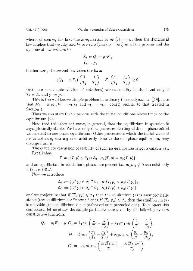
where, of course, the first one is equivalent to ml(0) = ms, then the dynamical law implies that m2, E2 and V2 are zero (and m x = me) in all the process and the dynamical law reduces to

E1 = Q1 -- plF1,

1;?1 = E l ;

furthermore, the second law takes the form

( Q I - P l F 1 ) ( ~ 1 ) ( P - ~ P ~ ) Ta +F1 _>0

(with our usual abbreviation of notations) where equality holds if and only if T1 = Ta and Ps = P~.

This is the well known simple problem in ordinary thermodynamics ([18], note that E1 = mlel,V1 = relY1 and rrh = me =const), similar to that treated in Section 4.

Thus we can state that a process with the initial conditions above tends to the equilibrium (*).

Note that this does not mean, in general, that the equilibrium in question is asymptotically stable. We have only that processes starting with one-phase initial values tend to one-phase equilibrium. Other processes in which the initial value of m2 is not zero, starting even arbitrarily close to the one-phase equilibrium, may diverge from it.

The complete discussion of stability of such an equilibrium is not available yet. Recall that

r -~- {(T,p) E %91 N%92 [/Zl(T,P) : ~2(T,P)}

and an equilibrium in which both phases are present i.e. mlm2 7 k 0 can exist only if (Ta,p~) E P.

Now we introduce

A1 := {(T,p) e %91 CI %92 [ /Zl(T,p ) < #2(T,p)},

/k2 :---- {(T,p) E %91 N %92 [ ]AI(T,P) > ]z2(T,p)}

and we conjecture that if (Ta,Pa) 6 z51 then the equilibrium (,) is asymptotically stable (the equilibrium is a "normal" one), if (Ta,p~) E A2 then the equilibrium (*) is unstable (the equilibrium is a superheated or supercooled one). To support this conjecture, let us study the simple particular case given by the following system constitutive functions:

{/AI(T1 , Pl) \

1) ;) + A12mlm2

Ta +612mlm2 Pl /72 '

876 T. Matolcsi Z A M P

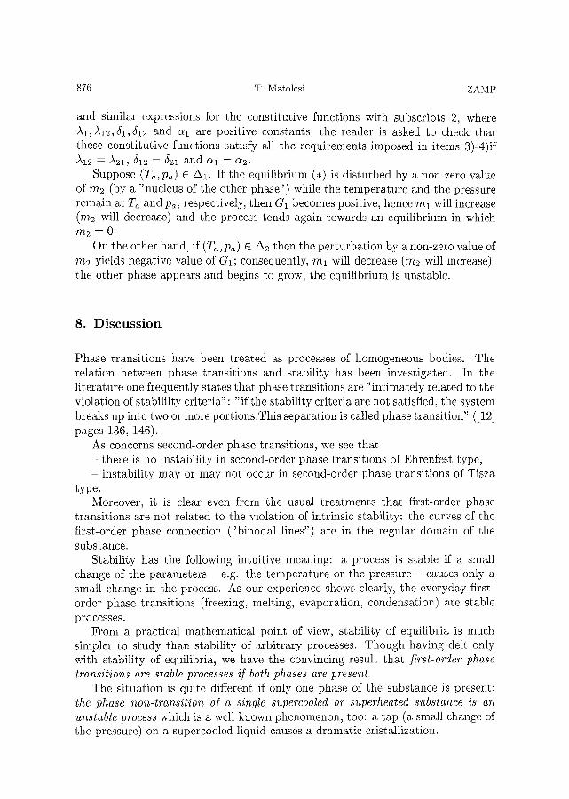
and similar expressions for the constitutive functions with subscripts 2, where A1, A12,51,612 and o~ 1 are positive constants; the reader is asked to check that these constitutive functions satisfy all the requirements imposed in items 3)-4)if /~12 = "~21, 612 = 621 and a l = a2.

Suppose (Ta,p~) E A1. If the equilibrium (.) is disturbed by a non-zero value of rn2 (by a "nucleus of the other phase") while the temperature and the pressure remain at Ta and Pa, respectively, then G1 becomes positive, hence ml will increase (m2 will decrease) and the process tends again towards an equilibrium in which ~Tt2 ~ 0.

On the other hand, if (Ta,p~) E A2 then the perturbation by a non-zero value of rn2 yields negative value of Gx; consequently, ml will decrease (rn2 will increase): the other phase appears and begins to grow, the equilibrium is unstable.

8. D i s c u s s i o n

Phase transitions have been treated as processes of homogeneous bodies. The relation between phase transitions and stability has been investigated. In the li terature one frequently states that phase transitions are "intimately related to the violation of stabililty criteria": "if the stability criteria are not satisfied, the system breaks up into two or more portions.This separation is called phase transition" ([12] pages 136, 146).

As concerns second-order phase transitions, we see that - there is no instability in second-order phase transitions of Ehrenfest type, - instability may or may not occur in second-order phase transitions of Tisza

type. Moreover, it is clear even from the usual treatments that first-order phase

transitions are not related to the violation of intrinsic stability: the curves of the first-order phase connection ("binodal lines") are in the regular domain of the substance.

Stability has the following intuitive meaning: a process is stable if a small change of the parameters e.g. the temperature or the pressure - causes only a small change in the process. As our experience shows clearly, the everyday first- order phase transitions (freezing, melting, evaporation, condensation) are stable processes.

From a practical mathematical point of view, stability of equilibria is much simpler to study than stability of arbitrary processes. Though having delt only with stability of equilibria, we have the convincing result that first-order phase transitions are stable processes if both phases are present.

The situation is quite different if only one phase of the substance is present: the phase non-transition of a single supercooled or superheated substance is an unstable process which is a well known phenomenon, too: a tap (a small change of the pressure) on a supercooled liquid causes a dramatic cristallization.

Vol. 47 (1996) On the dynamics of phase transitions 87Y

Our results show clearly that only the appearance of a new phase is a phenomenon related to instability and support the well known qualitative explanation of nucleation as a result of "infinitesimally small density fluctuation" ([21], [15] p.162) If only one phase is present, a new phase does not begin to grow till a nucleus (a "f luctuated port ion") of tha t phase is not stabilized. If nucleation is hindered somehow and the process of the body crosses the curve of phase connection then an unstable equilibrium can be produced.

It is worth remarking the following. The states between the binodal line and the spinodal line the superheated states and the supercooled ones - lie in the regular constitutive domain i.e. the conditions of intrinsic stability are satisfied; they are usually called metastable ([15],[21],22]), and according to our results they are unstable. This confusion of"s table-metas table-unstable" is based on the improper use of the notion "s ta te" . Namely, the state of a body is a triplet ( e ,v ,m) : the couple (e, v) is not a state. The conditions of intrinsic stability are satisfied at all (e, v) in a phase. Considering a one-body system, we see tha t an equilibrium (e, v, m) is

- asymptot ical ly stable if (e, v) is over the binodal line (which in our notations means ( T ( e , v ) , p ( e , v ) ) C A1),

- unstable if (e,v) is under the binodal line, i.e. (e,v) is metastable in the usual terminology (in our notations (T(e, v), p(e, v)) E A2).

Appendix

Let n be a positive integer and suppose F is a continuously differentiable function from R = into N~ and consider the differential equation

= F ( x ) ,

moreover suppose tha t Xo is in the domain of F and

r ( x o ) = 0.

Then the constant function x(t) = Xo (t E IFt) is a solution of the differential equation, called an equilibrium.

We say tha t a solution r starts from a subset H of the domain of F if r(0) is in H . The solution proceeds in H if r(t) E H for all t _> 0.

An equilibrium Xo is stable if for each neighbourhood N of Xo there is a neighbourhood U of zo such that for every solution r s tart ing from U proceeds in N.

An equilibrium Xo is asymptotically stable if it is stable and there is a neighbourhood V ,of xo such tha t for all solutions r start ing from V we have limt-~oo r(t) = Xo.

A set E of equilibria is strictly asymptotically stable ([24]) if every equilibrium in E is stable,

- every equilibrium in E has a neighbourhood V such tha t if r is a solution star t ing from V then limt~oo r(t) is in the closure of E.


If L is a differentiable real valued function defined in ]R ~ then its derivative

(gradient) L ' is a function from R ~ into R ~. The real valued function ~(z) := L'(x) �9 F(x) defined in ]~n (where the dot stands for the inner product in R ~) is called the derivative of F along the differential equation.

The following two results are well known in stability theory ([23]).

1. If Xo is an equibrium and there is a continuously differentiable real valued function L, defined in a neighbourhood of Zo such that

(i) L has a strict local maximum at Xo, i.e. L(x) < L(xo) for all x in a neighbourhood of Xo,

(ii) ~ has a (strict) local minimum at Xo, then the equilibrium zo is (asymptotically) stable.

2. If Xo is an equilibrium and there is a continuously differentiable real valued function L, defined in a neighbourhood of Xo such that

(i) L has not a local maximum at Zo,

(ii) ~ has a strict local minimum at Zo, then the equilibrium zo is unstable.

L is usually referred to as a Lyapunov function. The third, less common result concerning strict asymptot ic stability ([25], Sec-

tion 34) reads in a convenient reformulation as follows.

3. Let H be the set of all equilibria and suppose (i) there are a non-trivial linear subspace Z in IR ~, an element a of R ~ such

tha t H = (a + Z) C? DomF, (ii) for all Zo r H,

- KerF ' (xo) = Z, - the algebraic multiplicity and the geometric multiplicity of the zero eigen-

value of F~(Xo) are equal, - the real par t of the non-zero eigenvalues of F~(xo) is negative.

Then H is strictly asymptotical ly stable.

P r o p o s i t i o n A. Let C and B n x n real matrices such that (i) B is symmetric and negative semidefinite,

(ii) C is symmetric and positive definite. Then

- the algebraic multiplicity and the geometric multiplicity of every eigenvalue of C B are equal,

- the non-zero eigenvalues of C B are negative.

Proof. C -1 is symmetr ic and positive definite as well. Then < ~, 7 /> := (C-1~) .r/ defines an inner product on 1R ~. C B is symmetric and negative semidefinite with respect to this new inner product for

< ~ , c B v > = ( c - 1 ~ ) �9 (CBv) = ,~. B ~ = ( B ~ ) �9 v = < c B ~ , v >

Vol. 47 (1996) On the dynamics of phase transitions

and < ~, CB~ >= ~. B~ < 0

which implies our assertion ([26], Section 78).

879

R e f e r e n c e s

[1] J.W.Cahn and J.E.Hilliard, Acta Metall. 19 (1971), 151-161. [2] J.Carr, M.E.Gurtin and M.Slemrod, Arch.Rat.Mech.Anal. 86 (1984), 1984. [3] S.W.Koch , Dynamics of First-Order Phase transitions in Equilibrium and Nonequilibrium

Systems, Lecture Notes in Physics, 207, Springer, Berlin 1984. [4] R.Hagan and J.Serrin, Dynamic Changes in a van der Waals Fluid, New Perspectives in

Thermodynamics, Ed. J.Serrin, Springer, Berlin 1986 241-260. [5] ts and I.Pawlow, Physica D 59(1992), 389-416. [6] M.E.Gurtin, Arch.Rat.Mech.Anal. 123 (1993), 306-333. [7] M.Brokate, N.Kenmochi, I.Mtiller and J.E.Rodriguez, Phase transitions and Hysteresis,

Springer, Berlin 1994. [8] G.R.Gavalas, Nonlinear Differential Equations of Chemically Reacting Systems, Springer,

Berlin 1968. [9] M.J.Pilling, Reaction Kinetics, Clarendon Press, Oxford 1974.

[10] C,G.Hammes, Principles of Chemical Kinetics, Academic Press, New York 1978. [11] P.t~rdi and J.T6th, Mathematical Models of Chemical Reactions, Princeton Univ. Press

1989. [12] L.Szili and J.T6th, Phys. Rev, E 48 (1993), 183 186. [13] Nigel Goldenfeld, Lectures on Phase Transitions and the Renormalization Group, Addison-

Wesley, New York 1992, p. 29. [14] T.Matolcsi, ZAMP 47 (1996), 837 857. [15] H.B.Callen, Thermodynamics, John Wiley and Sons, New York 1960. [16] N.Boccara, Les principes de la thermodynamique classique, Press Univ. de France, Paris

1968, p. 60. [17] J.T~llieu, La thermodynamique, Press Univ. de France, Paris 1990 p. 71. [18] T.Matolcsi, Phys.Ess. 5 (1992), 320-327. [19] T.Matolcsi, Phys.Ess. 6 (1993), 158-165. [20] T.Matolcsi, Phys. Ess. 8 (1995), 15-19. [21] S.W.Koch, Dynamics of First-Order Phase Transitions in Equilibrium and Non-equilibrium

Systems, LNPh.207, Springer, Berlin 1984. [22] V.P.Skripov, J.Non-equ.Therm. 17 (1992), 193-236. [23] N.Ronche, P.Hubets and M.Laloy, Stability Theory by Lyapunov's Direct Method, Springer,

Berlin 1977. [24] T.Matolcsi, PU.M.A. Ser.B 3 (1992), 37-43 . [25] J.G.Malkin, Theorie der Stabilitiit einer Bewegung, Akademie-Verlag, Berlin 1959. [26] P.l~.Halmos, Finite Dimensional Vector Spaces, Springer, Berlin 1974.

Department of Applied Analysis EStvSs Lorgnd University 1088 Mfizenm krt 6-8. Hungary E-maih matolcsi~ludens.elte.hu

(P~eceived: November 17, 1995; revised: May 25, 1996)

on the dynamics of phase transitions -...

Documents