On the Efficiency of Fluid Simulation of Networks

Daniel R. Figueiredo1 Benyuan Liu2 Yang Guo3 Jim Kurose1 Don Towsley1 ∗

1Dept. of Computer Science 2Dept. of Computer Science 3The MathWorksUniversity of Massachusetts University of Massachusetts Natick, MA 01760Amherst, MA 01003 Lowell, MA 01854 yguo@mathworks.com{ratton, kurose, towsley} bliu@cs.uml.edu@cs.umass.edu

Computer Science Technical Report 04-82

September 24, 2004

Abstract

Performance evaluation of computer networks through traditional packet-level simulation is becoming in-creasingly difficult as networks grow in size along different dimensions. Due to its higher level of abstraction,fluid simulation is a promising approach for evaluating large-scale network models. In this study we focus onevaluating and comparing the computational effort required for fluid- and packet-level simulation. To measurethe computational effort required by a simulation approach, we introduce the concept of “simulation event rate,”a measure that is both analytically tractable and adequate. We identify the fundamental factors that contributeto the simulation event rate in fluid- and packet-level simulations and provide an analytical characterization ofthe simulation event rate for specific network models. Among such factors, we identify the “ripple effect” as asignificant contributor to the computational effort required by fluid simulation. We also show that the parameterspace of a given network model can be divided into different regions where one simulation technique is moreefficient than the other. In particular, we consider a realistic large-scale network and demonstrate how the com-putational effort depends on simulation parameters. Finally, we show that flow aggregation and WFQ schedulingcan effectively reduce the impact of the “ripple effect.”

Keywords: fluid simulation, packet simulation, performance evaluation, network models

1 Introduction

Packet-level simulation is a commonly used approach for evaluating the performance of computer networks. How-

ever, with the increasing size of networks such as the Internet, packet-level simulation has become computationally

expensive and in many cases infeasible. Consequently, there is an important need for more efficient simulation

techniques for large-scale network models.∗This research has been supported in part by the NSF under awards ANI-9809332, ANI-0085848 and EIA-0080119, and in part by

CAPES (Brazil). Any opinions, findings, and conclusions or recommendations expressed in this material are those of the authors and do notnecessarily reflect the views of the National Science Foundation

1

Many methods have been proposed to speed up the simulation of traditional network models. These methods

can be loosely placed into three orthogonal categories (see Figure 1): computational power; simulation technol-

ogy; and simulation model. Simulations can be sped up by using more powerful processors or processor arrays.

Improved simulation technology in the form of enhanced algorithms, such as the calendar queue and lazy queue

algorithms [4, 18], have been proposed to speed up event-list manipulation. Techniques based on importance sam-

pling or the RESTART mechanism can facilitate rare event simulation [10, 20]. The third dimension – simulation

model – entails the development of network models that have higher levels of abstraction; this requires fewer events

to be simulated and, thus, improves efficiency. For example, the packet-train simulation technique models a cluster

of closely-spaced packets as a single “packet-train” [1]. Although these techniques can result in significant simu-

lation speed up, there is often a concomitant loss in the accuracy of various performance measures, as the timing

among closely-spaced packets is lost in the abstraction.

Computational Power

Simulation Technology

Simulation Model

Faster CPUMultiprocessor

Efficient EventList Algorithm

Higher Abstraction LevelSimpler Model

Figure 1: Different dimensions in speeding up simulations

Fluid modeling is a modeling abstraction in which network traffic is represented as a continuous fluid flow,

rather than a sequence of discrete packet instances. This modeling technique was initially applied by Anick et al.

to analytically model data network traffic [2]. Fluid models can also be simulated instead of solved analytically.

Roughly speaking, while a packet-level simulator must keep track of all individual packets in the network, a fluid-

level simulator must keep track of the fluid rates at all traffic sources and network queues.

The higher level of abstraction of fluid-level simulation suggests that it might require much less computational

effort than a packet-level simulation, since a large number of packets can be represented by a single fluid flow.

We will see later in this paper, however, that this need not always be the case. The complex dynamics of fluids

that contend for resources in a queue can significantly increase the computational effort needed in a simulation,

negating the benefits of a high abstraction level.

In this paper we investigate the dynamics of fluid simulation and characterize the computational effort required

to simulate common network models. We then compare the effort required by traditional packet-level and fluid-level

simulation. We introduce a measure known as the simulation event rate to characterize the computational effort

2

required by a given simulation. For some scenarios considered, we derive analytical results for the event rates of

both fluid- and packet-level simulations. We identify the major factors that contribute to the event rates of both

approaches, such as the ripple effect, and establish the influence of model parameters such as source transmission

rates and number of sources on the event rate. We also consider a realistic large-scale network model and analyze

it in detail to characterize the dynamics of fluid simulation.

The remainder of this paper is organized as follows. Section 2 briefly presents related work in this area.

Section 3 discusses the dynamics of fluid- and packet-level simulation. In Section 4, tandem network models are

presented and analyzed. Section 5 considers cyclic network models. In Section 6, we evaluate the efficiency of

a large-scale network model and discuss the tradeoffs involved in fluid simulation. In Section 7, we show that

flow aggregation and a WFQ (Weighted-Fair Queueing) policy can reduce the fluid simulation event rate. Finally,

concluding remarks are presented in Section 8.

2 Related Work

Fluid models have been widely used to evaluate the performance of large-scale networks, with much of the work

focusing on analytical solutions and some on simulations [2, 14, 11, 12, 13, 3, 8]. In the area of fluid simulation,

researchers have investigated both continuous- [13] and discrete-time simulation [11, 12], and both pure [11, 12, 13]

and hybrid fluid models [3, 8]. Much of the emphasis in this past work has been on calculating performance

metrics (e.g., throughput) [15, 14, 17] and comparing these results with those obtained using equivalent packet-

level models. As with any higher-level modeling abstraction, fluid models present a potential compromise in

simulation accuracy. However, many results have suggested that the loss in accuracy is usually small [15, 14, 13].

A related topic, which is the focus of this paper, is the relative efficiency of fluid- and packet-level simulation,

i.e., the characterization and comparison of the computational cost of simulating a given network model using fluid

and packet-level simulation. Kesidis et. al were the first to investigate this issue using numerical experiments with

actual simulators [11]. Subsequent work has also focused on numerical comparisons between the running time

of both simulation approaches [13, 8]. Our work differs from these prior studies in that we focus on the analyt-

ical characterization of the computational effort and on the impact of model parameters on simulation efficiency

[12]. We consider exact and discrete simulation of fluid models with open-loop traffic sources. We view this as a

fundamental step in exploring the full potential of fluid simulation.

3 Dynamics of Fluid Simulation

In this section we introduce a measure for the computational effort of simulations and describe the dynamics of

sources and multiplexers of both fluid- and packet-level models. The dynamics of these building blocks are crucial

3

for understanding the computational cost of simulating large network models.

3.1 Simulation Event Rate

In order to compare the efficiency of fluid- and packet-level simulation, we must establish a common metric for

the computational effort required by both approaches. Clearly, the time required to execute each simulation is the

ultimate comparison metric, since it directly reflects the computational effort required. However, this metric is not

easily obtained analytically, and cannot be measured without actually running the simulation. Moreover, simulation

execution times can be both implementation and machine dependent. Thus, we introduce a more fundamental

measure to represent the computational effort required by a simulation, namely its simulation event rate, defined

as:

E = limt→∞

N(t)t

(1)

where N(t) is the total number of events that occur in the simulator by time t. In a packet-level simulation,

events include source transitions, packet generation at sources and packet departures from queues. In fluid-level

simulations, events include source transitions and fluid rate changes at sources and queues. This metric represents

the average number of events that the simulator processes per unit of simulated time. The intuition is that simulation

events are directly related to the computational effort involved in simulating a particular model. Different events

will incur different computational costs, and these differences may vary from one simulator implementation to

another. However, assuming that each event has some constant computational cost and considering all events during

the execution of a simulation, we expect the simulation event rate to be a good indicator of the overall amount of

computational effort required. Indeed, as we will see, the execution time of a given simulation is proportional to its

corresponding event rate.

3.2 Source Models

Due to their wide-spread use in the networking research literature, we will consider Markovian on-off sources as

the traffic generation model. Such traffic sources are often used to capture the bursty nature of network traffic and

can be easily combined to form more complex sources. Moreover, the on-off source model can be used in both

packet and fluid models and has been widely studied in both contexts [19].

The on-off source consists of two states: on and off. State holding times are assumed to be exponentially

distributed random variables with means 1/λ and 1/µ, respectively. In the packet model, a source generates packets

according to a Poisson process with rate γ when in the on state. In the fluid model, the source generates fluid at

a constant rate h. Neither packets nor fluids are generated when a source is in the off state. In order for a fluid

source to be considered equivalent to a packet source, we minimally require that they have the same average data

4

rate. Given this requirement, the constant fluid rate is h = γx, where x is the average packet size of a packet source

(without loss of generality, we assume that packets have a fixed size). Figure 2 illustrates the behavior of the on-off

packet and fluid sources.

Both fluid- and packet-level simulators must keep track of the state of on-off sources and schedule events for

source state transitions. In addition, the packet-level simulator must generate one simulation event for each packet

generated by the source, while the fluid simulator must generate a simulation event only when a source’s fluid rate

changes.

on off

�

�Packet

Sourceonoff

Fluid

Figure 2: On-off sources (packet and fluid)

3.3 Multiplexers

The second, more interesting, basic network component is the multiplexer. An important characteristic of a multi-

plexer is its scheduling discipline. We consider two scheduling disciplines in this paper: FIFO and WFQ (Weighted

Fair Queueing). The dynamics of FIFO scheduling are described below, while WFQ is presented in Section 7.2.

We start by revisiting the classic FIFO packet model, where packets arrive to a queue at discrete points in time

and are placed in a buffer. Packets stored in the buffer are served from the queue in the order of their arrival and

depart the queue at discrete points in time. Assume there are N packet sources feeding a FIFO queue with service

rate c, and that packets arrive to the queue at time instants τ1 < τ2 < · · · . The dynamics of the queue size can be

described by q(t) = A(t)−D(t). Where A(t) = argmaxi≥1{t : τi < t} represents the number of arrivals in time

(0, t) and D(t) represents the number of departures in time (0, t). Figure 3 depicts a FIFO queue being fed by two

sources. Note that while packet departures occur in the same order as packet arrivals, their inter-packet spacings

may change.

������������ ���������

Source 2

Source 1

time

Input Queue Output

Figure 3: Dynamics of a FIFO packet multiplexer

The dynamics of the FIFO fluid multiplexer are much more subtle. First, note that fluids from two different

5

sources are distinct and do not mix in the queue, just as packets transmitted by two sources are differentiated within

the queue. Fluids from different sources may be arriving simultaneously at a queue (which cannot occur in the

packet-level model) and the FIFO fluid queue can serve fluids from multiple sources simultaneously (again, unlike

the packet-level queue). Due to this complexity, we provide a formal description of the dynamics of the fluid FIFO

queue.

Assume there are N fluid sources feeding a FIFO queue with service capacity c. Let ak(t) and dk(t) be the fluid

arrival and departure rates (amount of fluid arriving/departing the queue per time unit) of the k-th source at time t.

The aggregate fluid arrival rate at the queue is given by a(t) = ∑Nk=1 ak(t). Suppose that the aggregate fluid arrival

rates to the queue change at times τ1 < τ2 < · · · . The dynamics of the queue size, q(t), can be described by the

following recursive equation:

q(t) = max(0, q(τi)+(a(t)− c)(t − τi)) , τi ≤ t < τi+1

We can also describe the fluid departure rate of the k-th source as a function of the fluid arrival rates. Note

that the departure rate of a fluid flow depends not only on its own arrival rate, but on those of all other flows as

well. A departing fluid flow shares the queue’s service capacity with all other flows currently being FIFO-served in

proportion to their arrival rates. There are two possible scenarios to consider when the aggregate flow arrival rate

changes at time τi:

• q(τi) = 0. In this case, the arrival rate change results in an immediate change in the departure rate, since nofluid is backlogged in the queue. There are two subcases to consider:

– a(τi) ≤ c. In this case, the departure rate of each source is equal to its arrival rate, dk(τi) = ak(τi).

– a(τi) > c. In this case, a backlog will begin to form at time τi. For a FIFO queue, each source willreceive service at a rate proportional to its arrival rate, thus, dk(τi) = c ak(τi)/a(τi).

• q(τi) > 0. In this case, the fluids backlogged at τi must first be served before the arrival rate change at timeτi is reflected in a changed departure rate. There are again two subcases to consider:

– a(τi) > c. In this case, once the backlog q(τi) is served, the departure rate of flow k will be given byc ak(τi)/a(τi). Thus, dk(τi +q(τi)/c) = c ak(τi)/a(τi).

– a(τi)≤ c. In this case, although the aggregate arrival rate at τi is less than or equal to the service capacityof the queue, the fluid that arrives while the current backlog q(τi) is being served will accumulate inthe queue. Hence, after the current backlog is served, the new corresponding departure rate of source kwill be dk(τi +q(τi)/c) = c ak(τi)/a(τi). Note that dk(τi +q(τi)/c) > ak(τi) for all k, i.e., the departurerate of fluid that arrived at time τi will be larger than its arrival rate. This newly created backlog willeventually be completely served and the departure rate for each source will drop to its instantaneousarrival rate at that moment. Since it takes (a(τi)q(τi)/c)/(c− a(τi)) time units to completely servethis newly accumulated backlog, we have d(τi + q(τi)/c +(a(τi)q(τi)/c)/(c−a(τi))) = ak(τi), for allt such that τi +q(τi)/c+(a(τi)q(τi)/c)/(c−a(τi)) ≤ t < τi+1. Note that depending on the time of thenext arrival rate change, τi+1, this rate change may not occur.

6

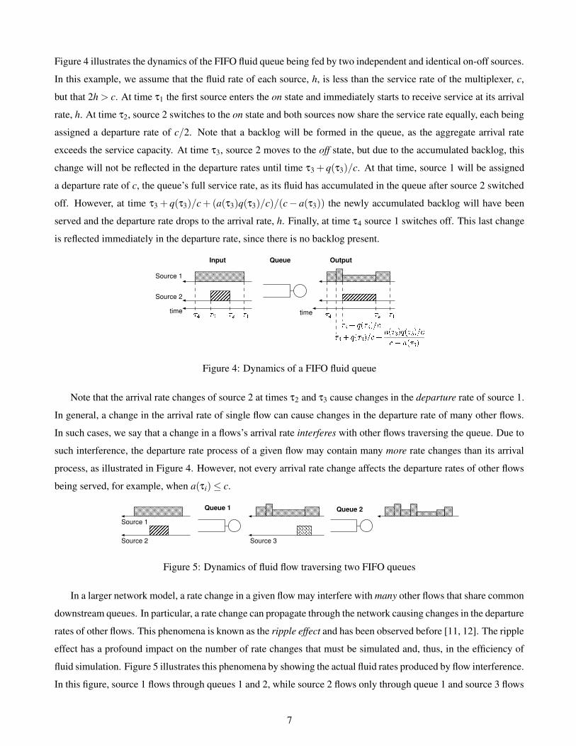
Figure 4 illustrates the dynamics of the FIFO fluid queue being fed by two independent and identical on-off sources.

In this example, we assume that the fluid rate of each source, h, is less than the service rate of the multiplexer, c,

but that 2h > c. At time τ1 the first source enters the on state and immediately starts to receive service at its arrival

rate, h. At time τ2, source 2 switches to the on state and both sources now share the service rate equally, each being

assigned a departure rate of c/2. Note that a backlog will be formed in the queue, as the aggregate arrival rate

exceeds the service capacity. At time τ3, source 2 moves to the off state, but due to the accumulated backlog, this

change will not be reflected in the departure rates until time τ3 + q(τ3)/c. At that time, source 1 will be assigned

a departure rate of c, the queue’s full service rate, as its fluid has accumulated in the queue after source 2 switched

off. However, at time τ3 + q(τ3)/c +(a(τ3)q(τ3)/c)/(c− a(τ3)) the newly accumulated backlog will have been

served and the departure rate drops to the arrival rate, h. Finally, at time τ4 source 1 switches off. This last change

is reflected immediately in the departure rate, since there is no backlog present.

���������� �Source 2

Source 1

time

Input Queue Output

!�"$#&%(')!�"+*-,/.time

0�132&4(5)0�1+6-798:2 ; 5)0�1+6<4(5)0�1=6-7/88?> ; 5)0 1 6

@�AB�CD E

Figure 4: Dynamics of a FIFO fluid queue

Note that the arrival rate changes of source 2 at times τ2 and τ3 cause changes in the departure rate of source 1.

In general, a change in the arrival rate of single flow can cause changes in the departure rate of many other flows.

In such cases, we say that a change in a flows’s arrival rate interferes with other flows traversing the queue. Due to

such interference, the departure rate process of a given flow may contain many more rate changes than its arrival

process, as illustrated in Figure 4. However, not every arrival rate change affects the departure rates of other flows

being served, for example, when a(τi) ≤ c.

Source 2

Source 1

Queue 1 Queue 2

Source 3

Figure 5: Dynamics of fluid flow traversing two FIFO queues

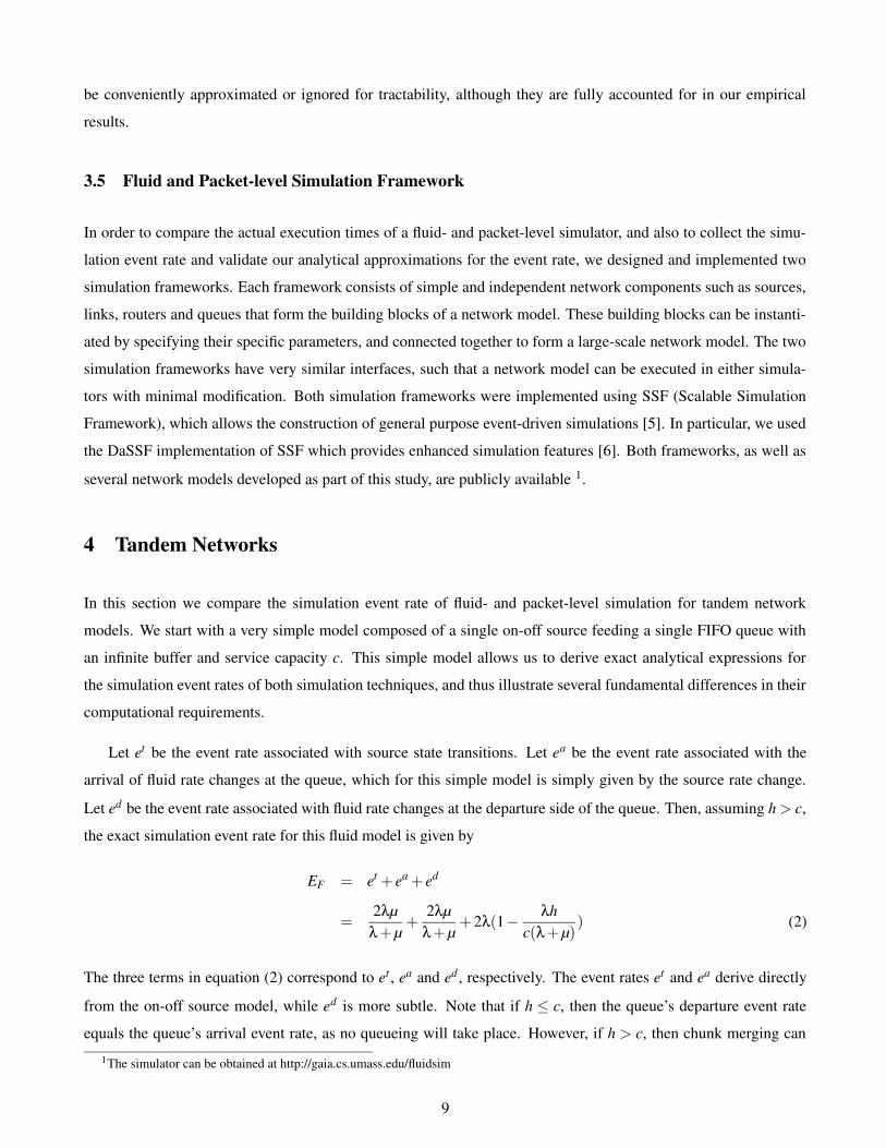
In a larger network model, a rate change in a given flow may interfere with many other flows that share common

downstream queues. In particular, a rate change can propagate through the network causing changes in the departure

rates of other flows. This phenomena is known as the ripple effect and has been observed before [11, 12]. The ripple

effect has a profound impact on the number of rate changes that must be simulated and, thus, in the efficiency of

fluid simulation. Figure 5 illustrates this phenomena by showing the actual fluid rates produced by flow interference.

In this figure, source 1 flows through queues 1 and 2, while source 2 flows only through queue 1 and source 3 flows

7

only through queue 2. We observe that the number of rate changes in the departure rate of flow 1 at queue 2 is

much larger (8 rate changes) than the number of rate changes at the source (2 rate changes).

3.4 Events in Fluid Simulation

The discrete-time simulation of a packet-level FIFO queue is straightforward since packets are handled individually.

The simulation of a fluid FIFO queue, however, is much more complicated since the arrival rates of all flows must

be maintained during periods that the queue is backlogged, as illustrated in the above example. To perform this

bookkeeping, we introduce the notion of fluid chunks. A fluid chunk Ci is defined as the set of fluid arrival rates

that changed at time τi. Flows traversing the queue that did not change their arrival rates at time τi are not part of

fluid chunk Ci. Since several arrival rates can change simultaneously, the fluid chunk need not be a singleton set.

Note that fluid chunk Ci will be reflected at the departure side of the queue when the backlog q(τi) has been served.

If the queue is empty (q(τi) = 0) at the time the fluid chunk is formed, then it is processed immediately.

Unfortunately, this definition of fluid chunk is not sufficient to handle all the events associated with a fluid FIFO

queue. In particular, recall from our discussion above that when q(τi) > 0 and a(τi) ≤ c, a change in the departure

rate of fluids can occur without any changes to its arrival rates. In this case, we need a special event that will change

the departure rate of the fluids after the backlog is served. Figure 6 illustrates the fluid chunks that are formed when

simulating the example shown in Figure 4. Note that a special event must be scheduled at time τ3 as the departure

rate of source 1 will first change to c (the full capacity of the queue), which occurs when C3 is processed, and only

change to h after the backlog is served.

special event

Source 2 : h

FHGSource 1 : h

IKJat LNMat O�P

Source 1 : hat QSRT

Source 1 : 0

U$Vat WYX

Source 2 : 0at ZS[\^]

Figure 6: Different fluid chunks of a FIFO queue

An important property of fluid chunks is the fact that two consecutive chunks can merge in the queue. Chunk

merging occurs in the following scenario: Assume a queue has a backlog q(τi) when the fluid rate of flow k changes

from h to zero at time τi. At this instant a fluid chunk Ci is formed. Now suppose that at time τi+1 the same flow k

changes its fluid rate back to h. A new fluid chunk, Ci+1 will then be formed at the queue. However, if τi+1 < q(τi)/c

then Ci can be discarded and need not be processed by the simulator. In this case, we say that the two consecutive

on periods of flow k have merged in the queue.

Special events and chunk merging can impact the computational effort required by fluid simulation and the

number of events simulated. However, in most cases the impact of special events and chunk merging is very small.

In particular, the probability that such events occur during simulation decreases as the size of the simulated model

increases (e.g., in number of sources, higher loads, etc). In the analytical evaluation that follows, these events will

8

be conveniently approximated or ignored for tractability, although they are fully accounted for in our empirical

results.

3.5 Fluid and Packet-level Simulation Framework

In order to compare the actual execution times of a fluid- and packet-level simulator, and also to collect the simu-

lation event rate and validate our analytical approximations for the event rate, we designed and implemented two

simulation frameworks. Each framework consists of simple and independent network components such as sources,

links, routers and queues that form the building blocks of a network model. These building blocks can be instanti-

ated by specifying their specific parameters, and connected together to form a large-scale network model. The two

simulation frameworks have very similar interfaces, such that a network model can be executed in either simula-

tors with minimal modification. Both simulation frameworks were implemented using SSF (Scalable Simulation

Framework), which allows the construction of general purpose event-driven simulations [5]. In particular, we used

the DaSSF implementation of SSF which provides enhanced simulation features [6]. Both frameworks, as well as

several network models developed as part of this study, are publicly available 1.

4 Tandem Networks

In this section we compare the simulation event rate of fluid- and packet-level simulation for tandem network

models. We start with a very simple model composed of a single on-off source feeding a single FIFO queue with

an infinite buffer and service capacity c. This simple model allows us to derive exact analytical expressions for

the simulation event rates of both simulation techniques, and thus illustrate several fundamental differences in their

computational requirements.

Let et be the event rate associated with source state transitions. Let ea be the event rate associated with the

arrival of fluid rate changes at the queue, which for this simple model is simply given by the source rate change.

Let ed be the event rate associated with fluid rate changes at the departure side of the queue. Then, assuming h > c,

the exact simulation event rate for this fluid model is given by

EF = et + ea + ed

=2λµ

λ+µ+

2λµλ+µ

+2λ(1−λh

c(λ+µ)) (2)

The three terms in equation (2) correspond to et , ea and ed , respectively. The event rates et and ea derive directly

from the on-off source model, while ed is more subtle. Note that if h ≤ c, then the queue’s departure event rate

equals the queue’s arrival event rate, as no queueing will take place. However, if h > c, then chunk merging can

1The simulator can be obtained at http://gaia.cs.umass.edu/fluidsim

9

occur and changes in the departure fluid rate will occur only when the queue is empty and the source is off. The

parenthesized term within the expression for ed gives the exact probability that the queue is empty and the source is

in the off state. This joint probability can be computed using the technique presented in [2]. Given that the source

is off, the rate at which the source changes its transmission rate is simply λ. Since a busy period is followed by an

idle period, we actually have two rate changes.

The simulation event rate for the packet level simulation is simply given by:

EP =2λµ

λ+µ+

2γµλ+µ

(3)

The first term in (3) is identical to that of fluid simulation and represents the event rate associated with the source

transitions. The second term is the event rate for the packet arrival and departure events. This is simply twice the

source packet generation rate, since each packet creates both an arrival and departure event.

Given equations (2) and (3), we see that the fluid simulation event rate is less its packet-level counterpart if

γ > λ/µ(λ + 2µ−λh/c). Although not presented here, this analysis was confirmed by simulation results. There-

fore, for the single source, single queue case, a fluid simulation will require less computational effort than a cor-

responding packet-level simulation whenever the packet generation rate, γ, is sufficiently large. We will see next

however, that with multiple sources and multiple queues, this advantage is mitigated due to flow interference and

the consequent ripple effect. Note that the event rates associated with source transitions, et , are identical in both

simulation approaches and thus will be ignored in future comparisons.

4.1 Multiple Sources, Single Queue

We now extend the above model and consider the case in which a FIFO queue is fed by N statistically independent

and identical on-off sources. We assume there exists a k,1 ≤ k ≤ N, such that k γ ≤ c < (k + 1)γ, i.e., that k + 1

sources (or more) are required to be on in order for the queue to accumulate a backlog. Consider a single flow,

i, traversing this queue in the fluid model and the events that must be simulated. The flow arrival event rate is

identical to the single source case. The departure event rate is now more subtle due to flow interference. If the

queue is non-empty and flow i is in the on state, a rate change in any other flow will affect the eventual departure

rate of flow i. This occurs since the number of flows sharing of the link changes, thus creating a new flow chunk.

Similarly, if the queue is empty and flow i is on, the departure rate of flow i will change when more than k sources

are on. The following Proposition for the departure event rate of a fluid source summarizes this discussion:

Proposition 1 Consider N identical on-off sources flows feeding a FIFO fluid queue. Then, the departure event

rate of a flow traversing this queue is given by

ed = ea +α(N −1)ea +β (4)

10

where α is the probability that source i is in the on state and the queue is non-empty; and β is the rate at which the

queue transits from a non-empty to an empty period given that source i is on.

The quantities α and β can be computed numerically using techniques presented in [2]. Note that β is the rate

at which the queue changes from the empty state with k−1 sources being active (on) and source i being in the on

state, to the state where k sources and source i are on.

The proposition above ignores chunk merging and special events. By ignoring chunk merging, we overestimate

the event rate, while by ignoring special events, we underestimate the event rate. Although these quantities can

be non-negligible under certain circumstances (e.g., a small number of sources, low loads), we expect them to

be negligible for most interesting scenarios (e.g., a large number of sources, high loads). The quantitative results

below obtained through simulation support this conjecture.

From the proposition above, we have that the total fluid simulation event rate of the model is given by

EF(N) = N(ea + ed) = αN(N −1)ea +2Nea +Nβ (5)

The event rate in equation (5) has a quadratic dependency on N. This occurs because sources can interfere with the

departure rate of one another. However, this dependency will be mitigated if the queue is empty most of the time

(i.e., α is very small). To investigate this behavior we next consider some numerical results.

The packet simulation event rate is just N times the packet simulation event rate of the single source case, thus

EP = N2γµ

λ+µ(6)

Let ρ be the load of the queue, which is defined as the ratio of the average aggregate arrival rate to the service

rate of the queue. Thus, ρ = 1/c ∑Ni=1 hiµi/(λi + µi), where N is the number of sources traversing the queue and

hi,µi and λi are the parameters of source i. In the examples that follow, we let λi = µi = hi = 1, for all i.

In the first experiment we fix the service rate of the queue (c = 50) and vary the number of sources, N, from

2 to 95 (which corresponds to loads of 0.02 to 0.95). Figure 7(a) shows the fluid and packet simulation event rate

as a function of N; both analytical results and a direct measurement of the fluid simulation event rate are shown

(γ = 5). The packet simulation event rate increases linearly, while the fluid simulation event rate exhibits two

different behaviors. For a small number of sources (which corresponds to low loads), the fluid simulation event

rate increases linearly, since interference among fluid flows is minimal. For a large number of sources, the event

rate increases dramatically as flow interference becomes significant. Recall that fluid flows interfere only when

the queue is non-empty and that the probability of a non-empty queue increases sharply as the load approaches 1.

Thus, fluid simulation has a higher computational cost at high loads. We will see shortly that the crossover point

will depend on the packet generation rate γ. Finally, we observe that the analytical expression for the fluid event

11

0

500

1000

1500

2000

2500

3000

3500

0 10 20 30 40 50 60 70 80 90 100

Packet (analytical)Fluid (analytical)Fluid (simulated)

Number of Sources

Sim

ulat

ion

Eve

nt R

ate

(a)

0

100

200

300

400

500

600

700

800

900

0 50 100 150 200 250 300Number of Sources

Sim

ulat

ion

Eve

nt R

ate

Packet (analytical)Fluid (analytical)Fluid (simulated)

Asymptote for Fluid

(b)

Figure 7: Simulation event rate of multiple sources traversing a single FIFO queue: (a) fixed service capacity; (b)

fixed load

rate from Proposition 1 (which ignores special events and chunk merging) closely matches the measured simulation

event rate.

We next fix the load (ρ = 0.8) and vary the number of sources from 2 to 295. In order to maintain a constant load

we scale the service rate of the queue from 1.25 to 184.375. The resulting fluid simulation event rate is shown in

Figure 7(b) together with the packet simulation event rate (γ = 3). Note that the fluid simulation event rate initially

grows linearly at one rate, and then converges to a second linear growth rate. The dashed line represents twice the

arrival event rate, which is the total event rate if no flow interference were to occur. Note that the analytical and

measured fluid simulation event rates exhibit similar behavior and converge to the value of twice the arrival event

rate. This convergence occurs because the probability that the queue is non-empty goes to zero as the number of

sources increases and the load remains constant. Under this scenario, the probability of flow interference goes to

zero and the departure event rate becomes equal to the arrival event rate.

4.2 Multiple Sources, Multiple Queues

We further generalize the above single queue model and consider a tandem queueing network formed by a sequence

of queues and multiple sources. This scenario is of interest since complex tandem networks can generally be

decomposed into various intersecting tandem queues whose structure provides for a tractable analytical evaluation

of the fluid simulation event rate.

0 1

(N-1)(K-1)

P0 P0 P0

P P (N-1)0 P P (N-1)1

... K-1P0 P0

P11 --10 -- 1K -- P

Figure 8: A tandem queueing network

12

Our tandem queueing network model of K FIFO queues is depicted in Figure 8. A single on-off source enters

the first queue and traverses all other queues. Each queue is additionally fed by N − 1 identical and independent

additional on-off sources that leave the system after traversing that queue. Although, this system has many param-

eters, two parameters – the number of sources entering each queue (N) and the number of queues in the system (K)

– are the most important, since they have direct influence on flow interference and the ripple effect.

We can approximate the fluid simulation event rate by considering one queue at a time. Let qi be the event rate

at queue i,0 ≤ i < K. Then:

q0 = N(ea + edr (0)) (7)

qi = (N −1)(ea + edr (i))+ ed

s (i−1)+ eds (i) (8)

where ea is the arrival event rate from a single on-off source to a queue, eds (i) is the departure event rate at queue i

of the source that traverses all queues, and edr (i) is the departure event rate of a single cross-traffic source (that exits

after one queue) at queue i. We can easily compute ea as in the single queue case, while the departure event rates

are given by

edr (i) = ea +α(ed

s (i−1)+ ea(N −2))+β (9)

eds (i) = ed

s (i−1)+αea(N −1)+β (10)

where we let eds (−1) = ea. Note that α and β actually depend on i. In the above equations, we consider an

approximation where α is the probability that a given source is in the on state and the queue is non-empty, and β is

the rate at which the queue transits from a non-empty to an empty state given that a particular source is on. This

approximates the effects of flow interference. We can solve the recursion in equation 10 and obtain

eds (i) = ea +αea (i+1)(N −1)+β (i+1) (11)

Thus, the fluid simulation event rate can be approximated by

EF(K) =K−1

∑i=0

qi (12)

= 2NKea +(N −1)2Keaα+(N −1)K2eaα+(N −1)2K(K −1)eaα2/2 (13)

where we have ignored the contribution of β. As in the single queue case, this approximation also ignores flow

merging and events associated with special chunks. Note that the fluid simulation event rate, EF(K), depends

quadratically on the number of queues in the tandem system and on the number of flows traversing the queues.

This quadratic behavior is a manifestation of the ripple effect, which increases as the number of queues or sources

increase. However, we will see shortly that another fundamental quantity – the probability the queue is non-empty

– can mitigate this quadratic growth.

13

The packet-level simulation event rate is much simpler to calculate. Its exact form is given by:

EP(K) = KN2µγ

λ+µ(14)

Note that this is simply KN times the packet rate of each source, with each packet generating two events (arrival

and departure) at each queue. As expected, the event rate is linear in each of K and N.

In order to illustrate the tradeoffs, we simulate an instance of the tandem model above. We first consider the

impact of K, the number of queues in the tandem system, on the simulation event rate, for N = 15 sources with

λ = µ = 1 for all sources and ρ = 0.8. Figure 9(a) shows the fluid and packet simulation event rate (for γ = 25).

We observe that the fluid simulation event rate increases quadratically with the number of queues in the system, as

predicted by our analysis, while the packet simulation event rate exhibits a linear increase. Note that if the network

is small enough, fluid simulation can be more efficient, despite its quadratic dependence on K. Also, as for the

single queue case, fluid simulation can be more efficient if γ is sufficiently large. Other models, with differing

number of sources entering each node, also exhibit similar qualitative behavior.

0

20000

40000

60000

80000

100000

120000

0 10 20 30 40 50 60 70 80 90 100

Packet (analytical)Fluid (analytical)Fluid (simulated)

Number of Queues

Sim

ulat

ion

Eve

nt R

ate

0

2000

4000

6000

8000

10000

12000

14000

16000

0 10 20 30 40 50 60 70 80 90 100 110 120 130 140 150 160 170 180 190Number of Sources

Sim

ulat

ion

Eve

nt R

ate

Packet (analytical)Fluid (analytical)Fluid (simulated)

Asymptote for Fluid

(a) (b)

Figure 9: Simulation event rate of a tandem system: (a) as a function of the number of queues (fixed N = 15, load

ρ = 0.8, γ = 25), (b) as a function of the number of sources (fixed K = 20, load ρ = 0.8, γ = 4)

The second important parameter to consider is N, the number of flows entering each queue, as this affects the

interaction among different flows. We consider the same scenario as above, but with K = 20 queues. We maintain

a constant load (ρ = 0.8) for all simulations by increasing the service rate of the queues as N increases. Figure 9(b)

presents the results obtained for this scenario for γ = 4. Surprisingly, the fluid simulation event rate increases sub-

linearly with the number of sources and then approaches a linear increase equal to twice the arrival event rate of all

sources in the system. Note that the analytical and measured fluid simulation event rate have very similar behavior,

and both approach the same asymptotic value. The explanation for the sublinear growth and the asymptotic value

is similar to that of the single queue case – the probability that flows interfere with one another goes to zero at

constant load as the number of sources increases. Since the packet-level simulation exhibits a linear increase, the

14

fluid simulation will have a smaller event rate than its packet counterpart for large enough values of γ.

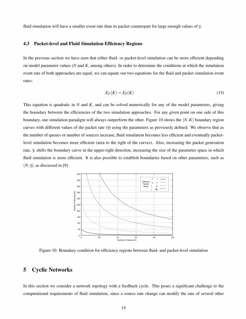
4.3 Packet-level and Fluid Simulation Efficiency Regions

In the previous section we have seen that either fluid- or packet-level simulation can be more efficient depending

on model parameter values (N and K, among others). In order to determine the conditions at which the simulation

event rate of both approaches are equal, we can equate our two equations for the fluid and packet simulation event

rates:

EF(K) = EP(K) (15)

This equation is quadratic in N and K, and can be solved numerically for any of the model parameters, giving

the boundary between the efficiencies of the two simulation approaches. For any given point on one side of this

boundary, one simulation paradigm will always outperform the other. Figure 10 shows the (N,K) boundary region

curves with different values of the packet rate (γ) using the parameters as previously defined. We observe that as

the number of queues or number of sources increase, fluid simulation becomes less efficient and eventually packet-

level simulation becomes more efficient (area to the right of the curves). Also, increasing the packet generation

rate, γ, shifts the boundary curve in the upper-right direction, increasing the size of the parameter space in which

fluid simulation is more efficient. It is also possible to establish boundaries based on other parameters, such as

(N,γ), as discussed in [9].

0

50

100

150

200

250

300

350

400

450

500

0 20 40 60 80 100Number of Queues (K)

Num

ber o

f Sou

rces

(N)

_�`badc_�`fegc_�`bahegc_�`ji)ckc

DifferentPacketRates

Figure 10: Boundary condition for efficiency regions between fluid- and packet-level simulation

5 Cyclic Networks

In this section we consider a network topology with a feedback cycle. This poses a significant challenge to the

computational requirements of fluid simulation, since a source rate change can modify the rate of several other

15

flows, with these rate changes propagating forward to other queues in a cycle, creating additional rate changes and

resulting in a cascading effect. Indeed, in such scenario, one might expect the simulation event rate to grow without

bound, with the simulator processing simultaneous rate changes in queues forming a cycle without ever advancing

simulation time.

S1

S2

S3

S4

H1

H2

H3

H4

Figure 11: A cyclic network model with a feedback cycle

In order to investigate the simulation event rate in a network with a feedback cycle we consider the cyclic

system depicted in Figure 11. This scenario contains four identical, infinite buffer FIFO queues connected together

in a cycle. An on-off source generates traffic into each of the queues. The routing of the flows is such that each

flow traverses exactly three queues before departing the system: three different flows thus traverse each queue. The

four traffic sources are identical, having equal on and off periods and a peak rate equal to 1. The stability condition

of this system requires each service rate to be greater than 1.5, the average aggregate arrival rate to each queue.

5.1 Packet-level simulation of the cyclic network

A cyclic model does not introduce any special considerations into a packet-level simulation. A packet generated at

a source simply traverses the queues, and leaves the system without introducing additional events in other packet

flows. When the system is stable (load < 1), the simulation event rate is independent of the service rate and link

propagation delay. The packet-level simulation event rate for the model in Figure 11 is thus fully determined by

the source packet rate and the number of nodes a flow traverses, and is given by:

EP = (es + eqNq)Nn (16)

where es denotes the event rate of a single source; eq is the per-source event rate of the queue; Nq is the number of

queues traversed by each flow; and Nn is the total number of nodes in the system. The event rate associated with

each flow is given by es + eqNq. Since each node introduces a single source into the system, the overall event rate

is given by equation (16). This equation was verified against simulation results (not presented here) and proved to

be a very good estimate of the measured event rate.

16

In order to evaluate the system under different loads, we vary the service rate of the queues from 1.6 to 3.1,

which corresponds to system loads of 0.94 to 0.48, respectively. The link propagation delay will also be varied,

taking values of 0.001, 0.01, 0.1 and 1 time units. Note that neither of these parameters influence the packet-level

simulation event rate, but, as we will see, are fundamental in determining the event rate of fluid-level simulation.

Equation (16) was used to plot the packet-level simulation event rates for γ = 1,5,10 in Figure 12 (solid lines).

5.2 Fluid-level simulation of the cyclic network

It is not easy to obtain an accurate closed form approximation for the fluid simulation event rate in cyclic network

models, as the cyclic nature of the topology creates complex dynamics in the flow’s rate change process. Thus, we

consider the event rate of the fluid cyclic network through simulation only.

20

40

60

80

100

120

140

160

180

200

220

1.6 1.8 2 2.2 2.4 2.6 2.8 3 3.2Service Rate

Sim

ulat

ion

Eve

nt R

ate

lnm^odp

qnrts

unvxw

delay 1.0delay 0.1delay 0.01delay 0.001

Figure 12: Simulation event rate for the cyclic network model

Using our simulator, we measured the fluid simulation event rate and observed that it converged to a finite value

under all scenarios considered. The results are shown in Figure 12 as a function of the service rate of the queues.

Each staircase shaped curve corresponds to a different link propagation delay. Given our discussion above about the

cascading (ripple) effect in fluid cyclic networks, it may seem surprising that the simulation event rate converged

at all. Recall, however, that an arrival flow rate change will not cause other flows to change their departure rates

if the queue is empty and the aggregate arrival rate into the queue is smaller than its service rate. Thus, even in a

cyclic queueing system, a flow rate change will only cause a finite number of new rate changes at “downstream”

queues, if the joint probability that a queue is empty and the instantaneous aggregate arrival rate is smaller than the

service rate is greater than zero. Under this condition, a flow rate change will eventually arrive at a queue at which

no other flow will suffer a departure rate change, terminating the ripple effect.

The above condition for obtaining a finite event rate is directly related to the queue’s service rate. Interestingly,

the service rate has two opposite effects. First, as the service rate increases, the average queueing delay decreases,

making fluid rate changes propagate faster through the cyclic network. This effect tends to increase the event rate,

since more fluid rate changes occur within a fixed time interval. On the other hand, a larger service rate implies

17

that the queue is more likely to be empty and have an instantaneous aggregate arrival rate that is smaller than its

service rate, resulting in a larger probability that a fluid rate change will not interfere with other flows or propagate

downstream. This consideration reduces the simulation event rate. The combination of these two opposite effects

determines the fluid simulation event rate. Thus, as shown in Figure 12, the simulation event rate can both increase

and decrease with an increase in the service rate.

Another important factor with a direct impact on the fluid simulation event rate of cyclic network models is

the link propagation delay. A smaller link delay will require less time for a flow rate change to propagate to the

next queue and consequently, further downstream. This results in more flow rate changes per unit of time, causing

an increase in the overall simulation event rate. Therefore, for a fixed service rate, the simulation event rate will

increase as the link delay decreases, as shown in Figure 12.

An interesting characteristic of the simulation results are the two discontinuities in the event rate at service

rates 2 and 3. To understand this phenomena, recall that the probability that a rate change will interfere with other

flows is given by the probability that the queue is either not empty or is empty but has an instantaneous aggregate

arrival rate larger than the service rate. Now consider two service rates, one slightly less than 2, the other slightly

greater, denoted by (2− ε) and (2 + ε), where ε � 1. The probability that a queue is empty is approximately the

same for these two cases. Now we consider the probability that aggregate arrival rate is greater than service rate.

With a service rate of (2− ε), the aggregate arrival rate is larger than the service rate when two or more sources

are simultaneously on. In the four-queue cyclic network this probability is 11/16. When the service rate is (2+ ε),

the aggregate arrival rate is larger than the service rate only when at least three sources are simultaneously on; the

probability of this event is 5/16. Thus, the probability that a rate change interferes with other flows is much larger

when the service rate approaches 2 from the left than from the right, resulting in the discontinuity in the simulation

event rate evident in Figure 12. The discontinuity at service rate 3 can be explained using similar arguments.

Finally, a direct comparison between fluid- and packet-level simulation event rates again reveals that fluid

simulation is more efficient when the packet generation rate of the sources is sufficiently large. For the parameters

we consider, fluid simulation outperforms its packet-level counterpart when γ > 10, as illustrated in Figure 12.

Figure 13: A similar model with no cycles in the topology

In order to further investigate the impact of a cyclic network topology on the fluid simulation event rate, we

analyze a four-node tandem model that breaks the loop but is similar to the cyclic model considered above. This

tandem model is illustrated in Figure 13. To maintain the same load, two extra sources are added to the first queue,

which will also preserve the degree of interference among the flows. Figure 14 shows the results for both models

when the propagation delay is 0.001 (a parameter that has no impact on the simulation event rate of tandem network

18

models). We can observe that the event rate for the cyclic loop model is considerably larger than that of the tandem

model. This occurs because a single rate change event can generate rate changes that traverse the closed-loop

several times. This result indicates that a significant fraction of the simulation event rate is due to the topological

nature of the cyclic network model.

40

60

80

100

120

140

160

180

200

1.6 1.8 2 2.2 2.4 2.6 2.8 3 3.2

Service Rate

Sim

ulat

ion

Eve

nt R

ate

cyclic modelopen model

Figure 14: Simulation event rates: cyclic versus tandem network models

We noted earlier that an increase in the number of flows traversing a queue will result in an increase in the

simulation event rate, as flow interference becomes more prominent. In a cyclic network, this effect is magnified.

To illustrate this observation, we extend the model considered above to six queues and vary the number of queues

a flow traverses before leaving the system. The results are presented in Figure 15. As expected, the event rate

increases significantly as flow interference becomes more pronounced (as seen previously). The discontinuities

and the overall trend in the results are similar to four queue model discussed above.

0

200

400

600

800

1000

1200

1400

1600

1800

0.4 0.5 0.6 0.7 0.8 0.9 1

Load

Sim

ulat

ion

Eve

nt R

ate

2 hops3 hops4 hops5 hops6 hops

Figure 15: Simulation Event rate for a 6-node cyclic queue

5.3 Execution time and event rate

Thus far, we have used the simulation event rate as our sole measure of computational effort. In order to evaluate

the appropriateness and accuracy of the event rate as indicator of computational effort, we consider the execution

19

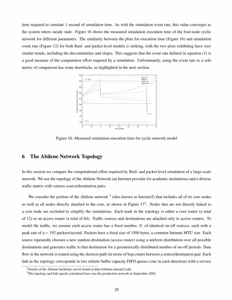
time required to simulate 1 second of simulation time. As with the simulation event rate, this value converges as

the system enters steady state. Figure 16 shows the measured simulation execution time of the four-node cyclic

network for different parameters. The similarity between the plots for execution time (Figure 16) and simulation

event rate (Figure 12) for both fluid- and packet-level models is striking, with the two plots exhibiting have very

similar trends, including the discontinuities and slopes. This suggests that the event rate defined in equation (1) is

a good measure of the computation effort required by a simulation. Unfortunately, using the event rate as a sole

metric of comparison has some drawbacks, as highlighted in the next section.

20

40

60

80

100

120

140

160

180

1.6 1.8 2 2.2 2.4 2.6 2.8 3 3.2Service Rate

Sim

ulat

ion

Exe

cutio

n Ti

me

(sec

)y{zt|~}

�n�^�

�n���

delay 1.0delay 0.1delay 0.01delay 0.001

Figure 16: Measured simulation execution time for cyclic network model

6 The Abilene Network Topology

In this section we compare the computational effort required by fluid- and packet-level simulation of a large-scale

network. We use the topology of the Abilene Network (an Internet provider for academic institutions) and a diverse

traffic matrix with various source/destination pairs.

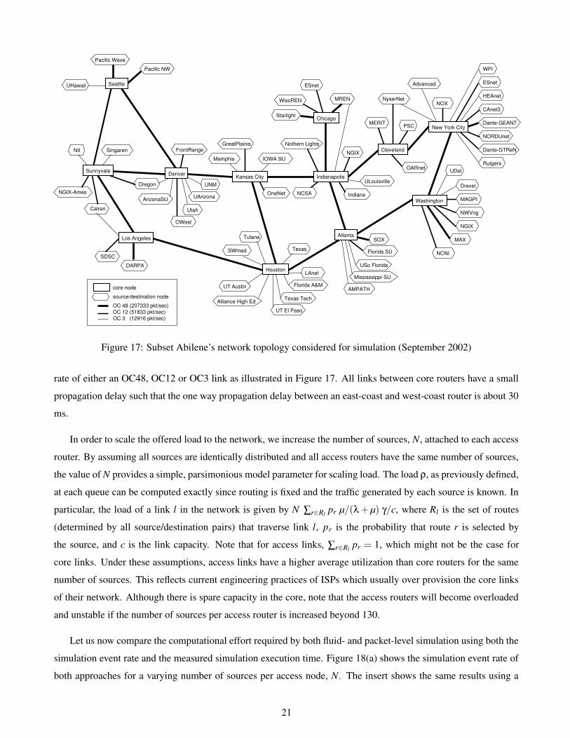
We consider the portion of the Abilene network 2 (also known as Internet2) that includes all of its core nodes

as well as all nodes directly attached to the core, as shown in Figure 173. Nodes that are not directly linked to

a core node are excluded to simplify the simulations. Each node in the topology is either a core router (a total

of 12) or an access router (a total of 64). Traffic sources and destinations are attached only to access routers. To

model the traffic, we assume each access router has a fixed number, N, of identical on-off sources, each with a

peak rate of γ = 192 packets/second. Packets have a fixed size of 1500 bytes, a common Internet MTU size. Each

source repeatedly chooses a new random destination (access router) using a uniform distribution over all possible

destinations and generates traffic to that destination for a geometrically distributed number of on-off periods. Data

flow in the network is routed using the shortest-path (in terms of hop count) between a source/destination pair. Each

link in the topology corresponds to two infinite buffer capacity FIFO queues (one in each direction) with a service

2Details of the Abilene backbone can be found at http://abilene.internet2.edu3The topology and link speeds considered here was the production network in September 2002.

20

Sunnyvale

Seattle

Denver

Los Angeles

Houston

Kansas City

Atlanta

Washington

Indianapolis

Chicago

Cleveland

New York City

Pacific NW

Pacific Wave

UHawaii

WPI

ESnet

HEAnet

CAnet3

Dante-GEANT

NORDUnet

Dante-GTReN

Rutgers

Advanced

NOXNyserNet

UDel

Drexel

MAGPI

NWVng

NGIX

MAX

NCNI

MERIT PSC

OARnet

WiscREN

ESnet

MREN

Starlight

ULouisville

Nothern Lights

NCSA Indiana

NGIX

Florida SU

USo Florida

SOX

Mississsippi SU

AMPATH

GreatPlainis

Memphis IOWA SU

OneNet

Florida A&M

Texas

LAnet

Texas Tech

UT El Paso

SWmed

UT Austin

Tulane

Alliance High Ed

UArizona

UNM

Utah

OWest

Oregon

ArizonaSU

FrontRangeNII

NGIX-Ames

Calren

Singaren

SDSC

DARPA

core node

source/destination node

OC 48 (207333 pkt/sec)OC 12 (51833 pkt/sec)OC 3 (12916 pkt/sec)

Figure 17: Subset Abilene’s network topology considered for simulation (September 2002)

rate of either an OC48, OC12 or OC3 link as illustrated in Figure 17. All links between core routers have a small

propagation delay such that the one way propagation delay between an east-coast and west-coast router is about 30

ms.

In order to scale the offered load to the network, we increase the number of sources, N, attached to each access

router. By assuming all sources are identically distributed and all access routers have the same number of sources,

the value of N provides a simple, parsimonious model parameter for scaling load. The load ρ, as previously defined,

at each queue can be computed exactly since routing is fixed and the traffic generated by each source is known. In

particular, the load of a link l in the network is given by N ∑r∈Rlpr µ/(λ + µ) γ/c, where Rl is the set of routes

(determined by all source/destination pairs) that traverse link l, pr is the probability that route r is selected by

the source, and c is the link capacity. Note that for access links, ∑r∈Rlpr = 1, which might not be the case for

core links. Under these assumptions, access links have a higher average utilization than core routers for the same

number of sources. This reflects current engineering practices of ISPs which usually over provision the core links

of their network. Although there is spare capacity in the core, note that the access routers will become overloaded

and unstable if the number of sources per access router is increased beyond 130.

Let us now compare the computational effort required by both fluid- and packet-level simulation using both the

simulation event rate and the measured simulation execution time. Figure 18(a) shows the simulation event rate of

both approaches for a varying number of sources per access node, N. The insert shows the same results using a

21

0

5e+06

1e+07

1.5e+07

2e+07

2.5e+07

0 20 40 60 80 100 120 140

Sim

ulat

ion

even

t rat

e

Number of sources

fluid simulationpacket simulation (measured)packet simulation (analytical)

10000

100000

1e+06

1e+07

1e+08

0 20 40 60 80 100 120 140

Sim

ulat

ion

even

t rat

e

Number of sources

0

20

40

60

80

100

120

140

160

0 20 40 60 80 100 120 140

Sim

ulat

ion

exec

utio

n tim

e (s

ec)

Number of sources

1

10

100

0 20 40 60 80 100 120 140

Sim

ulat

ion

exec

utio

n tim

e (s

ec)

Number of sources

fluid simulationpacket simulation

(a) (b)

Figure 18: Results for fluid- and packet-level simulation of the Abilene topology: (a) simulation event rate (b)

simulation execution time

log-scale for the vertical axis. As expected, the simulation event rate for the packet-level simulation (dotted line)

exhibits a linear increase, as increasing the number sources linearly increases the number of packets traversing the

network. The packet-level simulation event rate can again be closely approximated using equation (14), with a

value of K equal to the average number of hops between a randomly chosen source/destination pair. This analytical

result is also plotted in Figure 18(a) (dashed line).

The fluid simulation event rate exhibits linear growth with a much smaller slope up to about 100 sources. Note

that for this range, the event rate is about one and a half orders of magnitude smaller than that of the packet-

level simulation. However, when the number of sources increases beyond 110, the fluid simulation event rate

increases dramatically and eventually becomes larger than its packet-level counterpart. The cross over point occurs

at approximately 120 sources, which corresponds to an average access link utilization of 90%. This sharp increase

in the fluid simulation event rate is again due to the ripple effect, since flow interference increases with queue

utilization.

Figure 18(b) shows a direct comparison between the measured execution times of fluid- and packet-level simu-

lations of the Abilene topology. The insert shows the same results using a log-scale for the vertical axis. Again, we

consider the execution time required to simulate 1 second of simulation time. Although the execution times shows

a trend similar to their respective event rates, we can observe some important differences. First, the sharp increase

in the fluid simulation event rate is much larger (about 2 orders of magnitude) than the sharp increase in execution

time (about one order of magnitude). Second, when the number of sources is less than 100, the difference between

the execution time of fluid and packet-level simulation is less than one order of magnitude (as opposed to one and

a half orders of magnitude in the event rate). Such differences were not noticeable in the previous sections, where

the simulation event rate and execution time were much more closely related.

22

0

1e-05

2e-05

3e-05

4e-05

5e-05

6e-05

7e-05

8e-05

0 20 40 60 80 100 120 140

Eve

nt e

xecu

tion

time

(sec

)

Number of sources

fluid simulationpacket simulation

Figure 19: Average execution time of an event in fluid- and packet-level simulations

To help understand the causes of these differences we investigate the average execution time of an event as

a function of the number of sources for both fluid and packet-level simulations, as shown in Figure 19. Note

that the event execution time for packet-level simulation remains nearly constant as a function of the number of

sources. However, the event execution time for fluid simulation can vary significantly with load. This variation in

the execution time of an event (of up to a factor of 8) shows a limitation of using the simulation event rate as a

measure of the computational effort.

In a packet-level simulation, events such as packet arrivals and departures have a constant computational cost

independent of network load (assuming efficient event-list manipulation). Recall that all queues are FIFO and

packets either enter the tail of the queue or are removed from the head of the queue; thus, no queue-length dependent

computation is required to process either event. Moreover, the amount of memory consumed by an arrival event is

also constant, (as a single packet is allocated and placed in the queue) and every arrival event consists exactly of a

single packet.

Unfortunately, the same is not true for fluid simulation. Below we qualitatively discuss the factors that lead to

a load-dependent simulation event cost.

• Arrival event: Arrival events can occur simultaneously in a fluid queue. This happens when an upstreamqueue simultaneously changes the output rate of several flows and these flows enter the same downstreamqueue. Although each arrival rate change is counted as a single event, only a single fluid chunk (if any)will be created, and the cost of creating a fluid chunk containing i simultaneous arrivals will be less than itimes the cost of processing a single arrival. Moreover, the amount of memory required by a fluid chunk isproportional to the number of arrival rate changes that it contains.

• Departure event: Departure events can also occur simultaneously in a fluid queue. Recall that when a fluidchunk is processed, all flows in that chunk will suffer a departure rate change. Other flows that are currentlybeing serviced can also suffer a rate change as a consequence of processing the fluid chunk. Although eachdeparture rate change will count as one event (as with arrivals), the cost of processing a batch of departurerate changes will not be linear in the number of departure rate changes.

23

The variable processing cost of fluid events becomes more apparent when simulating large-scale networks, where

the number of flows traversing a queue can be very large. In the previous sections this variable cost was not

noticeable, as the number of flows considered was relatively small. In the Abilene scenario considered here, a

single core link (from node “Denver” to node “Kansas City”) can have up to 72,250 simultaneous flows (observed

in our simulations when N = 125).

0

10

20

30

40

50

60

70

80

90

0 20 40 60 80 100 120 140

Ave

rage

num

ber o

f flo

ws

depa

rting

a q

ueue

Number of sources

entire network

0

1

2

3

4

5

6

7

8

9

10

11

0 20 40 60 80 100 120 140

Ave

rage

num

ber o

f flo

ws

in a

chu

nkNumber of sources

entire network

(a) (b)

Figure 20: (a) Average number of flows departing a queue. (b) Average number of flows that form a fluid chunk

To quantitatively illustrate the variable cost of an event, we computed the average number of flows departing

a queue and the average number of flows that form a fluid chunk. Note that this metric is queue dependent and

we report on the average over all queues in the network. Figure 20 shows the result as a function of the number

of sources, N. Note that the average number of flows departing a queue increases linearly (Figure 20(a)) with an

increasing number of sources. This is expected as this metric reflects the average offered load to a queue. More

interesting is the behavior illustrated in Figure 20(b). The average chunk size is one when the number sources is

less than 90. Thus, for low utilization, a source rate change rarely interferes with any other flow in the network. As

the utilization increases above 90 sources, the chunk size increases dramatically. This occurs because a source rate

change now interferes with many other flows causing an arrival event in a downstream queue which itself is likely

to have a large number of flows, which leads to a large fluid chunk. Note that this increase in fluid chunk size is

independent of the ripple effect, and results only from high utilization. However, the ripple effect magnifies this

problem as rate changes will propagate large fluid chunks to downstream queues.

The increase in the number of flows traversing a queue helps explain why the execution time of an event

increases linearly when the number of sources is below 90 (Figure 19). In contrast, the large number of events

generated when the number of sources is above 90 helps explain why the execution time of an event decreases

sharply (Figure 19).

Another important consideration is the amount of memory required to run a simulation. Figure 21 illustrates

the total amount of memory required to simulate the Abilene topology using both the packet-level (dotted line)

and the fluid simulation (solid line). From the figure, we observe that in packet-level simulation the amount of

24

1

10

100

1000

10000

0 20 40 60 80 100 120 140

Am

ount

of m

emor

y re

quire

d (M

byte

s)

Number of sources

fluid simulationpacket simulation

Figure 21: Amount of memory consumed by the packet-level and fluid simulations

memory required increases linearly with the number of sources. This is expected, as the total memory required

is proportional to the average queue sizes, which is proportional to the load. As for the fluid-level simulation, the

simulator engine requires more memory than its packet-level counterpart even for very low levels of utilization.

This is due to the larger complexity needed in maintaining the simulation state. For example, a fluid chunk (which

has variable size) can be much larger in terms of bytes, than a packet-level data structure. Moreover, the memory

requirement for the fluid simulation increases dramatically as the utilization increases past 100 sources. This sharp

increase in the memory requirements is a direct consequence of the sharp increase in the fluid chunk size and on

the average number of chunks stored in a queue. The latter is a result of both the high utilization and of the ripple

effect.

Although the absolute values for the memory requirements of each simulation are implementation dependent,

the significance of such comparison lies in the trend of the curves. The fact that the memory required for fluid

simulation sharply increases at high utilization is also fundamental to fluid simulations and is not implementation

dependent.

A simulation’s execution time is a combination of the simulation event rate and the event execution time. We

have seen that at higher utilization, the ripple effect significantly increases the simulation event rate, which directly

impacts the execution time. Our above discussion shows that event execution time in fluid simulation can depend

on network utilization. This observation suggests that the simulation event rate may not be an accurate measure of

a simulation’s execution time in large-scale networks at very high loads.

7 Enhancements and Extensions

Our examples in the previous sections indicate that flow interference and its consequence, the ripple effect, can

significantly impact the efficiency of fluid simulation. In this section we consider two ways in which the efficiency

25

of fluid simulation can be improved. We first consider flow aggregation as a technique to reduce the amount of

flow interference. We then investigate the Weighted Fair Queueing (WFQ) scheduling policy, which by its nature

provides isolation among different flows and consequently reduces the amount of flow interference over FIFO

scheduling.

7.1 Flow Aggregation in Fluid Simulation

Flow aggregation, the bundling together background traffic into a single data flow, is a standard technique to reduce

the complexity of network models. The number of flows that are aggregated into a single flow can vary and a

network model can have several aggregated flows, each representing an aggregate of individual flows. In packet-

level simulation, flow aggregation does not reduce the number of events that must be simulated, as the simulator

must still keep track of each packet generated by the aggregate source. However, fluid simulation can benefit from

flow aggregation since flow interference will be reduced when fewer flows are present in the model.

a1

queue

d1

AggregatedArrival

a3

a2

d3

d2

DepartureAggregated

Figure 22: Example of flow aggregation

To illustrate the benefits of flow aggregation in fluid simulation, consider the example shown in Figure 22. The

figure shows three flows traversing a FIFO queue each with an arrival process corresponding to a1, a2 and a3. We

assume that h < c < 2h, such that the queue accumulates a backlog when two or more sources are on. The departure

processes of each flow are given by d1, d2 and d3, respectively. Suppose we aggregate the three flows into a single

flow. The arrival and departure process of the aggregate flow is also shown in Figure 22. Note that the number of

rate changes in the aggregated arrival process is equal to the sum of the rate changes in the arrival process of the

individual flows. Thus, flow aggregation does not change the event rate of the arrival process. However, there are

substantial reductions in the number of events in the departure process. In our example, the total number of rate

changes in the departure process of the individual flows is 11, while the aggregated departure process exhibits only

3 rate changes.

There are two important factors that lead to a large reduction in the number of rate changes in the departure

process of an aggregate flow. First, a single rate change in the departure process of the aggregated flow can

represent many simultaneous rate changes in the model with individual flows. Second, the probability that fluid

chunks merge in the queue increases. This occurs because aggregation bundles individual flows into a single larger

flow, increasing the chances for fluid chunks (that were separate in the case of individual flows) to be merged.

26

To generalize the above considerations, we present a simple approximate analysis of the fluid simulation event

rate when flow aggregation is used. Since the sources’ contributions to the overall simulation event rate are the

same in both the aggregated and non-aggregated scenarios, the following analysis only considers the event rate

associated with the departure process.

Recall the single FIFO queue fed by N on-off sources and the result in equation (4). Ignoring the last term (β),

the event rate of the departure process without flow aggregation can be approximated by:

EF = N ed

=2λµ

λ+µ(1−α+αN)N (17)

Suppose we are interested in the behavior of one of the sources traversing this queue, say the N-th source. We

can then create a model in which the N-th source shares the queue with an aggregate flow representing the other

N −1 sources. In this case, each rate change in the N-th flow can cause one rate change in the aggregated flow, and

each rate change in the aggregated flow can cause one rate change in the N-th flow. Let α′ denote the probability

that at least one source in the aggregated flow is on, α′ = 1− (1− µ/(λ + µ))N−1. Then, the total departure event

rate in this aggregated model, E′

F , can be approximated by:

E′

F =

[

2λµλ+µ

+2λµ

λ+µ(N −1)α

]

+

[

2λµλ+µ

(N −1)+2λµ

λ+µα′

]

(18)

The first bracketed term is the departure event rate of the N-th flow. The second bracketed term is the departure

event rate of the aggregate flow, which represents the other N −1 sources.

Equation (17) shows that in the worst case, the departure event rate increases quadratically with the number of

sources entering the queue. However, with flow aggregation the departure event rate increases linearly (Equation

(18)) with the number of sources being represented by the aggregate flow.

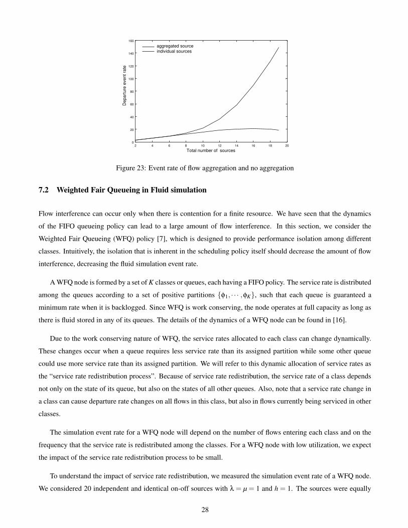
To demonstrate the potential of flow aggregation, we simulate and measure the departure event rate of the single

queue model presented above. All sources are identical with λ = µ = 1, and peak rate equal to 1. The service rate

of the infinite buffer FIFO queue is 10. The number of sources in the aggregate flow is varied from 1 to 18. Note

that the system becomes unstable when the total number of sources exceeds 19.

Figure 23 shows the departure event rate for both models as a function of the total number of sources. As

expected, the quadratic behavior in the event rate is indeed avoided when flow aggregation is used. Note that the

event rate with flow aggregation increases linearly for a certain range and decreases slightly after the number of

sources reaches 16. This reduction in the event rate is related to the increase in the chunk merging probability,

which was ignored in the analysis above, in equation (18).

27

0

20

40

60

80

100

120

140

160

2 4 6 8 10 12 14 16 18 20

aggregated sourceindividual sources

Total number of sources

Dep

artu

re e

vent

rate

Figure 23: Event rate of flow aggregation and no aggregation

7.2 Weighted Fair Queueing in Fluid simulation

Flow interference can occur only when there is contention for a finite resource. We have seen that the dynamics

of the FIFO queueing policy can lead to a large amount of flow interference. In this section, we consider the

Weighted Fair Queueing (WFQ) policy [7], which is designed to provide performance isolation among different

classes. Intuitively, the isolation that is inherent in the scheduling policy itself should decrease the amount of flow

interference, decreasing the fluid simulation event rate.

A WFQ node is formed by a set of K classes or queues, each having a FIFO policy. The service rate is distributed

among the queues according to a set of positive partitions {φ1, · · · ,φK}, such that each queue is guaranteed a

minimum rate when it is backlogged. Since WFQ is work conserving, the node operates at full capacity as long as

there is fluid stored in any of its queues. The details of the dynamics of a WFQ node can be found in [16].

Due to the work conserving nature of WFQ, the service rates allocated to each class can change dynamically.

These changes occur when a queue requires less service rate than its assigned partition while some other queue

could use more service rate than its assigned partition. We will refer to this dynamic allocation of service rates as

the “service rate redistribution process”. Because of service rate redistribution, the service rate of a class depends

not only on the state of its queue, but also on the states of all other queues. Also, note that a service rate change in

a class can cause departure rate changes on all flows in this class, but also in flows currently being serviced in other

classes.

The simulation event rate for a WFQ node will depend on the number of flows entering each class and on the

frequency that the service rate is redistributed among the classes. For a WFQ node with low utilization, we expect

the impact of the service rate redistribution process to be small.

To understand the impact of service rate redistribution, we measured the simulation event rate of a WFQ node.

We considered 20 independent and identical on-off sources with λ = µ = 1 and h = 1. The sources were equally

28

20

40

60

80

100

120

140

160

1 2 3 4 5 6 7 8 9 10

0.5 load0.8 load0.9 load

Number of Classes (subqueues)

Sim

ulat

ion

Eve

nt R

ate

�:�����

�:���

Figure 24: Simulation event rate as a function of the number of classes in a WFQ node

allocated to the classes, so that each class was fed by approximately the same number of sources. The number of

classes was varied from 1 to 10 and the service rate was distributed equally among the classes. The service capacity

of the node was set such that loads of 0.5, 0.8. and 0.9 were obtained. The simulation event rate of this model is

shown in Figure 24 as a function of the number of classes.

When the number of classes is one, the WFQ node behaves as a single FIFO queue. Note that at loads of 0.9

and 0.8, there is a sharp decrease in the simulation event rate when a FIFO node (single class WFQ) is replaced

by a 2-class WFQ node. The event rate further decreases as the number of classes in the WFQ node increases,

since increased performance isolation among the classes reduces the amount of flow interference. However, as

the number of classes increases beyond 7, the simulation event rate actually increases although the event rate to

simulate the WFQ node with any number of classes is always less than the event rate to simulate a FIFO node

with the same input flows. This occurs because the service rate redistribution process generates a larger number of

events when the number of classes increases.

As expected, when there is no queueing in the system (which occurs when the service rate is greater than or

equal to the sum of the peak rate of all the sources), the number of classes has no impact on the fluid simulation

event rate as shown in Figure 24 for a load of 0.5. We note that the inherent performance isolation among classes

in WFQ does not change the packet-level simulation event rate from the FIFO case. In the above model, the

packet-level simulation event rate is given by Equation (6).

The relative efficiency of fluid and packet-level simulation depends, as always, on the specific model parameter

values, especially γ, the packet rate at the sources. To illustrate, Figure 24 shows the packet-level event rate for

γ = 5,10. Note that fluid simulation can outperform packet-level simulation in some regions of the parameter

space. A more detailed analysis of the WFQ fluid simulation event rate is available in [9], which also discusses the

efficiency regions.

29

8 Conclusions

In this paper, we have analyzed the amount of computational effort required by fluid- and packet-level simulation

by exploring several different network models and using the simulation event rate as a measure of computational

cost. In fluid-level simulation, flow interference was found to be a fundamentally important property, inducing a

“ripple effect” that leads to larger simulation event rates. This phenomena is pronounced when considering large-

scale models with high utilizations. In the case of packet-level simulation, the source’s packet generation rates

were shown to be the parameter of fundamental importance. The simulation event rate can be easily determined

analytically and depends linearly on the number of packets generated. Thus, the relative efficiency between the two

simulation approaches depends critically on the ripple effect and the packet generation rates. We showed that flow

aggregation is an effective technique to reduce the amount of flow interference, reducing the impact of the ripple

effect and resulting in improved efficiency for fluid simulation. Different scheduling policies, such as WFQ, can

also have an impact on reducing flow interference and consequently improving the simulation event rate.

We also investigated the accuracy and adequacy of the simulation event rate as a measure of the computational

cost of a simulation. In all cases investigated, the trends shown by the simulation event rate matched the trends

shown by the execution time. However, as a result of the variability in the execution time of a fluid event, the

simulation event rate does not always accurately reflect the computational cost of large-scale network models at

high loads.

References

[1] Jong Suk Ahn and Peter B. Danzig. Packet network simulation: Speedup and accuracy versus timing granu-larity. IEEE/ACM Transactions on Networking, 4(5):743 – 757, October 1996.

[2] D. Anick, D. Mitra, and M.M. Sondhi. Stochastic theory of a data-handling system with multiple sources.The Bell System Technical Journal, 61(8):1871 – 1894, October 1982.

[3] Stephan Bohacek, Joao P. Hespanha, Junsoo Lee, and Katia Obraczka. A hybrid systems modeling frameworkfor fast and accurate simulation of data communication networks. In Proc. ACM SIGMETRICS 03, Jun 2003.

[4] Randy Brown. Calendar queues: a fast 0(1) priority queue implementation for the simulation event set prob-lem. Communications of the ACM, 31(10):1220 – 1227, 1988.

[5] S3 Consortium. Scalable simulation framework API reference manual. Documentation Draft, January 1999.

[6] J. Cowie, D. Nicol, and A. Ogielski. Modeling the global internet. Computing in Science & Engineering,pages 30–38, 1999.

[7] A. Demers, S. Keshav, and S. Shenkar. Analysis and simulation of a fair queueing algorithm. Internet Res.and Exper., 1, 1990.

[8] Yu Gu, Yong Liu, and Don Towsley. On integrating fluid model with packet simulation. In Proc. IEEEINFOCOM 04, March 2004.

30

[9] Yang Guo. On Fluid Modeling of Networks and Queues. PhD thesis, University of Massachusetts, Amherst -MA, 2000.

[10] Philip Heidelberger. Fast simulation of rare events in queueing and reliability models. ACM Transactions onModeling and Computer Simulation (TOMACS), 5(1):43–85, 1995.

[11] G. Kesidis, A. Singh, D. Cheung, and W.W. Kwok. Feasibility of fluid event-driven simulation for ATMnetworks. In Proc. IEEE GLOBECOM 96, volume 3, pages 2013–2017, November 1996.

[12] Benyuan Liu, Daniel R. Figueiredo, Yang Guo, Jim Kurose, and Don Towsley. A study of networks simulationefficiency: Fluid simulation vs. packet-level simulation. In Proc. IEEE INFOCOM 01, April 2001.

[13] Yong Liu, Francesco Lo Presti, Vishal Misra, Don Towsley, and Yu Gu. Scalable fluid models and simulationsfor large-scale ip networks. ACM Transactions on Modeling and Computer Simulation, 14(3), 2004.

[14] Vishal Misra, Wei-Bo Gong, and Don Towsley. A fluid-based analysis of a network of aqm routers supportingtcp flows with an application to red. In Proc. ACM SIGCOMM 00, September 2000.

[15] David Nicol, Michael Goldsby, and Michael Johnson. Fluid-based simulation of communication networksusing SSF. In Proc. 1999 European Simulation Symposium, Erlangen-Nuremberg, Germany, October 1999.

[16] Abhay K. Parekh and Robert G. Gallager. A generalized processor sharing approach to flow control in in-tegrated services network: The single-node case. IEEE/ACM Transactions on Networking, 1(3):344 – 357,June 1993.

[17] David Ros and Raymond Marie. Loss characterization in high-speed networks through simulation of fluidmodels. Telecommunication Systems, 16:73–101, Jan 2001.

[18] Robert Ronngren, Jens Riboe, and Rassul Ayani. Lazy queue: an efficient implementation of the pending-event set. In Proc. of 24th Annual Symposium on Simulation, pages 194 – 204, 1991.

[19] Mischa Schwartz. Broadband Integrated Networks. Prentice Hall, 1996.

[20] M. Villen-Altamirano and J. Villen-Altamirano. RESTART: a straightforward method for fast simulation ofrare events. In Proceedings of the 1994 Winter Simulation Conference, pages 282 – 289, Lake Buena Vista,Florida - USA, December 1994.

31