on the estimation of the price elasticity of electricity ... · jorge barrientos, esteban velilla,...

On the estimation of the price elasticity of electricitydemand in the manufacturing industry of Colombia

Jorge Barrientos, Esteban Velilla, David Tobón-Orozco, FernandoVillada and Jesús M. López-Lezama

Lecturas de Economía - No. 88. Medellín, enero-junio de 2018

Lecturas de Economía, 88 (enero-junio 2018), pp. 155-182

Jorge Barrientos, Esteban Velilla, David Tobón-Orozco, Fernando Villada and Jesús M. López-Lezama

On the estimation of the price elasticity of electricity demand in the manufacturing industry of Colombia

Abstract: This paper presents an estimation of the reaction of electricity demand to changes in price levels of forward contracts in themanufacturing industry of Colombia. To that end, a structural vector autoregressive (SVAR) model was developed, considering severaleconomic activities at different voltage levels. The industrial sectors under study showed an electricity demand not significantly sensitive to pricevariations. However, the food and drink sectors, plastic and rubber manufacturing, as well as retail trade turned out to be more sensitiveto price shocks than the chemical industry or textile manufacturing. Such inelasticity could be softened if information concerning prices andquantity demanded were of common knowledge, or if the forward curve were observable.

Keywords: electricity markets, forward contracts, price elasticity of demand, SVAR models.

JEL Classification: D43, D61, L13, L43, Q41.

Estimación de la elasticidad precio de la demanda de electricidad en la industria manufacturera de Colombia

Resumen: En este artículo se presenta una estimación de la reacción de la demanda a niveles de precios de contratos forward de electricidaden la industria manufacturera de Colombia. Se desarrolló un modelo de vectores autorregresivos estructurales (SVAR) considerando variasactividades económicas a diferentes niveles de tensión. Los sectores industriales bajo estudio no mostraron una demanda de electricidadsignificativamente sensible a variaciones de precios. Sin embargo, los sectores de alimentos y bebidas, caucho y plástico, así como el sectorcomercial minorista resultaron ser más sensibles a choques de precios que la industria química o el sector de manufactura de textiles. Dichainelasticidad podría suavizarse si la información concerniente a precios y cantidades demandadas fuera de conocimiento común, o si la curvaforward pudiera ser observable.

Palabras clave: mercados de electricidad, contratos forward, elasticidad precio de la demanda, modelos SVAR.

Clasificación JEL: D43, D61, L13, L43, Q41.

L’estimation de l’élasticité-prix de la demande d’électricité dans l’industrie manufacturière colombienne

Résumé: Cet article présente une estimation de la variation dans la demande d’électricité, due à des changements dans les niveaux deprix des contrats d’électricité du type forward, dans l’industrie manufacturière colombienne. Un modèle de vecteurs autorégressifs structuraux(SVAR) a été développé afin de considérer plusieurs secteurs économiques pour des différents niveaux de tension électrique. En général, lessecteurs industriels étudiés n’ont pas montré de demande d’électricité sensible aux variations de prix. Cependant, les secteurs de l’alimentationet des boissons, du caoutchouc et plastique, ainsi que le secteur du commerce de détail, se sont avérés être plus sensibles aux chocs des prix parrapport à l’industrie chimique et au secteur textile. Une telle inélasticité pourrait être adoucie si les informations concernant les prix et lesquantités demandées d’électricité étaient connues, ou bien si la courbe forward était observable.

Mots-clés: marchés d’électricité, contrats forward, élasticité-prix de la demande, modèles SVAR.

Classification JEL: D43, D61, L13, L43, Q41.

Lecturas de Economía, 88 (enero-junio), pp. 155-182 © Universidad de Antioquia, 2018

On the estimation of the price elasticity of electricity demand inthe manufacturing industry of Colombia

Jorge Barrientos, Esteban Velilla, David Tobón-Orozco, FernandoVillada and Jesús M. López-Lezama*

–Introduction. –I. The electricity market in Colombia. –II. Conceptual framework andmethods. –III. Empirical results. –Conclusions. –References.

doi: 10.17533/udea.le.n88a05

Original manuscript received on 31 January 2017; final version accepted on 18 July 2017

Introduction

The price elasticity of demand (PED) is one of the most important pa-rameters in economic analysis and practical econometrics, as it gives the per-centage change in the quantity demanded in response to a one percent change* Jorge Barrientos Marín: Associate Professor, Department of Economics, Universidad de An-

tioquia. Postal address: calle 70 N◦ 52-21 Medellín, Colombia.E-mail: [email protected] Velilla Hernandez : Assistant Professor, Department of Electrical Engineering, Uni-versidad de Antioquia. Postal address: Calle 70 N◦ 52-21 Medellín, Colombia.E-mail: [email protected] Tobón Orozco: Associate Profesor, Department of Economics, Universidad de Antio-quia. Postal address: calle 70 N◦ 52-21 Medellín, Colombia.E-mail: [email protected] Villada Duque: Associate Professor, Department of Electrical Engineering, Univer-sidad de Antioquia. Postal address: calle 70 N◦ 52-21 Medellín, Colombia.E-mail: [email protected]ús María López Lezama: Assistant Professor, Department of Electrical Engineering, Uni-versidad de Antioquia. Postal address: calle 70 N◦ 52-21 Medellín, Colombia.E-mail: [email protected].

Barrientos et al.: On the estimation of the price elasticity of electricity demand...

in price. Commodities such as oil and gasoline can be regarded as elastic inthe short run (Lin & Prince, 2013; Neto, 2012; Arzaghi & Squalli, 2015).These goods can be considered as produced and traded in competitive mar-kets. Nevertheless, there are some commodities, such as electricity power,which pricing behavior does not follow the usual patterns described in thecommodity pricing literature, so its PED could be more difficult to estimate.In the electric power industry, the study of demand elasticity serves to under-stand the reaction of consumers to price changes and the possibility that gen-erators exercise market power (Labandeira, Labeaga & López-Otero, 2016).Furthermore, the estimation of the PED in the electricity industry is impor-tant given the socio-economic impact that electricity has in contemporarysociety. Several factors have driven increasing interest in this issue in recentyears. Such factors include the trend of electricity deregulation in severalcountries (Arango & Dyner, 2006; Pollitt, 2009); new policies devised to mit-igate the environmental impact of energy resource exploitation (MacCombie& Jefferson, 2016; Nienhueser & Qiu, 2016); and a growing concern for en-ergy efficiency.

Demand estimation along with PED have been the focus of many studies.For example, industrial electricity demand studies are presented by Kamer-schen and Porter (2004) and Polemis (2007) for USA and Greece, using si-multaneous equations and cointegration methods, respectively.

Alter and Syed (2011) used cointegration and vector error correction todetermine the short- and long-run dynamics of electricity price and demand inPakistan. Beenstock, Goldin and Nabot (1999) adopted dynamic regressionand cointegration techniques to compute long-run elasticities in the house-hold and industrial sectors of Israel, while Bose and Shukla (1999) estimatedsectorial elasticities for small, medium and large firms employing a regres-sion approach. Agnolucci (2009) estimated electric energy demand and priceelasticity for German and British industrial sectors over the period 1978-2004using disaggregated data. Narayan and Smyth (2005), Halicioglu (2007) andZiramba (2008) used cointegration techniques to estimate the price elasticityof residential electricity demand in Australia, Turkey and South Africa, respec-tively; while Alberini and Fillippini (2011) applied partial adjustment modelsto estimate the price elasticity of household electricity demand in the USA.

158

159

Lijesen (2007) presented a study on real-time price elasticity of electricitydemand in the Netherlands. He provides a quantification of the real-timerelationship between total peak demand and spot market prices, finding a lowvalue of the real-time price elasticity, which might be explained by the factthat not all consumers observe spot market prices. In Thimmapuram et al.(2010) and Thimmapuram and Kim (2013), the modeling and simulation ofthe price elasticity of demand in Korea was carried out using a representativeagent-based model within a smart-grid environment. It is shown that beingwell equipped with smart grid technologies increases a consumer’s awarenessof responsiveness of demand. Also, a price-elastic consumer benefits from areduction in electricity usage and prices and contributes to reduce congestionas well as market power.

Bernstein and Madlener (2015) estimated electricity demand elasticitiesfor different subsectors of the German Manufacturing Industry from 1970 to2007; employing a cointegrated VAR approach and taking into account struc-tural breaks, they found long-run relationships among sectors and estimatedshort-run elasticities using a single-equation error correction modeling. Oka-jima and Okajima (2013) estimated the price elasticities of residential demandin Japan from 1990 to 2007. They found that the price elasticity of residentialelectricity demand in Japan is highly affected by income inequality and severeweather. Bernstein and Griffin (2006) estimated regional differences in priceelasticity in the US, finding that demand was relatively inelastic to price, andthat this relationship had not changed significantly between 1977 and 1999.Other studies regarding the estimation of elasticity of residential demand arepresented in Athukorala and Wilson (2010) and Arthur, Bond and Wilson(2012) for Sri Lanka and Mozambique, respectively.

Labandeira et al. (2012) use real data on prices and electricity consump-tion from Spain to present a model of incomplete information and in whichhouseholds and large consumers are taken into account to estimate the priceelasticity of electricity demand. The authors found that electricity demand isinelastic with respect to its price in the short term, although there are differ-ences between residential and industrial demand. In the case of households,demand elasticity diminishes as the level of per-capita income increases; how-ever, this relationship was not found in the case of large companies.

Lecturas de Economía -Lect. Econ. - No. 88. Medellín, enero-junio 2018


Cárdenas, Vásquez and Whittington (2014) performed a study regardingprice elasticity of the demand for electricity, oil and gas in Chile. They foundthat, among these goods, electricity is the most inelastic, with values rangingbetween -0.10 and -0.60 for the three mainmanufacturing sectors. Labandeiraet al. (2016) carried out a meta-regression analysis that intends to adjust theprice elasticities of electricity demand, identifying the main factors explainingthe differences between the results of the selected studies, such as country,type of consumers, data, models, sample period and estimation methods.

In this paper, we are interested in estimating the PED of electricity for-ward contracts in the manufacturing industry of Colombia. To this end, weperformed multivariate analysis. Initially, we used a vector autoregression(VAR); however, due to its poor performance in terms of the impulse re-sponse function (IRF), we used a structural vector autoregression (SVAR) toestimate the elasticity of demand and to simulate the response of demandto an impulse in the electricity price. The econometric analysis is based onmonthly observations of historical time series between 2005 and 2012, con-sidering economic activities (disaggregated up to two-digit International Stan-dard Industrial Classification codes) at different voltage levels. Our focus ison five electro-intensive sectors: food and drinks, plastic and rubber, retailtrade, textile manufacturing and chemical industry.

After an exhaustive survey of the existing literature on estimation of thePED in Colombia, we found out that this type of estimation has been rarelydone. To the best of our knowledge, this is the first paper that employs theVAR and SVAR approaches to estimate the PED in Colombia. The con-tribution of our paper can be summarized as follows: first, it adds to thesmall body of empirical literature on this matter in Colombia; second, it spec-ifies the relationship of industrial electricity demand as a function of elec-tricity prices, industrial production index, and hydrology; third, it providesconsistent estimations of the PED; and, finally, it computes (when possible)the IRF.

This paper is divided as follows. In section I, we describe Colombia’selectricity market and report some studies related to its electricity demandand PED. In section II, we introduce in a straightforward manner the VAR

160

161

and SVAR methodologies and describe the empirical strategy adopted for es-timating PED. In section III, we present and analyze our results. We concludewith a summary of the main conclusions.

I. The electricity market in Colombia

The electricity market in Colombia is composed of two main markets:a spot market and a bilateral market based on non-standardized contracts.An independent system operator (ISO) solves the ideal dispatch in the spotmarket. Rather than minimizing the hourly costs of generation, the objec-tive function of the ISO is to set an economic dispatch (twenty-four houroptimization problem), where generators submit bids and side payments areintroduced. The bids specify electricity offer prices for the next twenty-fourhours, startup costs and maximum generating capacity for each hour in thenext day. Once the optimization problem of the ideal dispatch is solved forthe twenty-four hours, the equilibrium price is calculated as the price bid ofthe marginal plant that is not saturated. The hourly spot price is defined asthe equilibrium price plus an uplift (De Castro et al., 2014).

Also, Colombia’s electricitymarket works on a 24-hour-ahead pool throughwhich all electricity is dispatched, regardless of any short-, medium- or long-term bilateral agreements between agents. These agreements are materializedin bilateral contracts called forward contracts. It is a stylized fact that electric-ity demand in this market does not change (or it does at a too slowly pace), andthis is especially evident in the spot market. Actually, the demand is a constant(a given fact) for setting the spot price, and, on the other hand, the marketsupply is built based on the daily-bid prices and the hourly-declared availabil-ity of the power generators. Therefore, in the electricity market of Colombia,the fundamental factors of short-term electricity pricing are hydrology as wellas the incentives and expectations of the agents and their strategies in the spotmarket. However, electricity pricing in the forward contract markets is verydifferent, and therefore the analysis of demand behavior and its response tochanges in prices is harder to investigate. While in the spot market there isperfect information about prices, forward contracts constitute private infor-mation for agents, so many variables are not directly observable. The only



available information consists of averages of prices and quantities demandedof energy in contracts. It is worth to mention that every forward contract isvery different in time and procedures. This paper focuses on the estimationof the PED for the electric power industry in such forward contract marketsin Colombia.

A forward contract is a financial instrument; more precisely, it is a powerpurchase agreement, which aims to protect agents from the risk to buy andsell at the spot market. In Colombia’s electricity market, there are two typi-cal agreements: consumption-based payment contract and Take or Pay con-tract. Their duration and price depends on the needs and bargaining powerof agents. In general, agents behave strategically and the choice to buy andsell energy in forward contracts or in spot markets is based on their privateinformation and the volatility of spot prices. This is because in both markets,even as they are trading exactly the same good, prices are dramatically differ-ent. This is one of the most criticized features of bilateral contract markets,because it makes the market very inefficient. In fact, any relationship betweencontract market price and hydrology vanishes, while that does not happen inthe spot market.

Few studies and analysis regarding electricity demand and the PED inColombia’s electricity market have been found. An exhaustive search in bib-liographic databases produced a few related papers that date back to the early1990s. For instance, Botero, Castaño and Vélez (1990) studied industrialelectricity demand in Colombia in the period 1970-1983. After not rejectingthe hypothesis of complementarity between electrical energy and the capitalstock, they carried out a parametric estimation of demand in terms of thecapital stock. According to these authors, the rational business decision ofthe firm is not to use electricity as input, as this is a direct consequence of theexistence of capital and the technical requirements inherent to the assumedproduction function. In fact, the decision problem of the firm is whetherto buy power from the grid or to be self-generating because the empiricalevidence suggests the existence of a substitution effect between these twoalternatives in the long run.

162

163

Ramírez (1991) developed a model in which the demand for electricity inColombia’s industrial sector is explained by the capital stock, the labor fac-tor and energy considerations. He splits the data into two groups: high andlow electricity consumption sectors. His results suggest that in the sectorof high electricity consumption, demand for electricity depends primarily onnon-energy factors; while in the low consumption sector, demand for elec-tricity depends on the conditions of energy as an input. These results confirmthe existence of complementarities between electricity and capital and substi-tutability between energy and labor due to the intensive and extensive use ofcapital in the first group (large companies) and the intensive use of labor inthe latter.

Barrientos, Olaya andGonzález (2007) presented a non-linear splinemodelfor demand estimation in the electricity market of Colombia. They modeledthe daily electricity demand in the southeast region of the country throughthe implementation of a non-parametric regression model. They consideredsome calendar variables such as time of the day, day of the week, month, andyear, among others, in the estimation process. Maddock and Castaño (1991)and Maddock, Castaño and Vella (1992) carried out estimates of residentialelectricity demand in Medellin (Colombia), where prices follow a rising blockscheme. They concluded that the price elasticity of demand is greater in thewell-off residential areas of the city. Franco, Velásquez and Olaya (2008) char-acterized monthly electric power demand in Colombia using a model of non-observable components from 1995 to 2006. They found that the monthlygrowth in demand has a linear deterministic component, approximately con-stant in recent years. Finally, Espinosa, Vaca and Ávila (2013) used an au-toregressive distributed lag model to estimate price elasticities of residentialand industrial demand in Colombia, finding that residential demand is moreinelastic than industrial demand.

II. Conceptual framework and methods

Multivariate time series analysis is an instrument for modeling variablesthat are correlated in time, unlike univariate models which do not allow suchan analysis. However, the ability to take multiple time series to be included



in a single model has drawbacks to be analyzed prior to use. For example, itis necessary to determine whether the various time series satisfy the covari-ance stationarity conditions, which are very important features for allowingidentification of the type of multivariate structure that has to be implemented.

If preliminary analysis of data indicates that the process is covariance-stationary (that is, the mean, variance and auto-covariance do not dependon the time in which the sample was taken), the typical procedure indicatesthat it is possible to use vector processes without restrictions on data, themost common of which are VAR models. However, if the process is notstationary, the suggested procedure consists of looking for long-run relationsbetween some (or all) of the variables, which necessarily leads to the notionof cointegration.1

Finally, it is important to highlight that VAR models also support theinclusion of exogenous variables as explanatory variables, but in this case it isnot possible to compute either the impulse-response function or the variancedecomposition. The inclusion of explanatory variables in the VAR just allowsone to compute the marginal effect on the endogenous variables.

A. Empirical Specification

In general, a VAR model can be written as:Yt = c+ Φ1Yt−1+Φ2Yt−2+ · · ·+ΦpYt−P+εt, (1)

where Yt = [y1t, y2t, . . . , ynt]′ is an n×1 vector for all t, εt is a white noise dis-

turbance term, thereforeΦj is a matrix of dimension n×n for j = 1, 2, . . . , p.Note that the inclusion of more variables and more lags could make the esti-mators very inefficient in terms of significance of the parameters. Moreover,if the number of parameters exceeds the number of observations, then theidentification conditions are not satisfied and it is not be possible to carry outthe estimations (Hamilton, 1994).1 Two time series are said to be cointegrated if each one separately is non-stationary (i.e., in-

tegrated of any order, possibly order 1), but there is a linear combination of the series thatis covariance stationary or of order zero (0). This indicates that the time series have commontrends, which can be either deterministic or stochastic.

164

165

The implicit assumptions of the VAR can be summarized as follows: first,for a covariance stationary process, matrices Φj , j = 1, . . . , p, in (1) can bedefined as the coefficients in the projection of Yt on p lags of Yt, so εt isnot correlated with Yt−j , j = 1, . . . , p, by the definition of Φ1,Φ2, . . . ,Φp.The parameters of the VAR can be consistently estimated by ordinary leastsquares by performing n independent regressions. Second, the assumptionthat Yt follows a pth-order VAR process is basically that p lags are sufficientto summarize all the dynamic correlations among elements of Yt. Under thestationarity assumption of every series in Yt, model (1) can be written as:

Yt= c+

∞∑s=1

Ψsεt−s, (2)

which is a vector autoregressive moving average process whereΨs is a n × nmatrix interpreted as the impulse-response function (IRF). It is easy to checkthat

∂yt+s

∂εt= Ψs. (3)

Thus, equation (3) admits the following interpretation: the element (i, j)of matrix Ψs identifies the consequences of an increase of a unit or one stan-dard deviation n the innovations εj at time t on the values of the variable yiin t+ s, holding constant the innovations in other times. It means that

∂yi, t+s

∂εj,t= Ψs =

∂yi,t+s

∂yjt. (4)

Assuming that yit represents the electricity demand at time t and yjt rep-resents its price, once the VAR is estimated we can compute the IRF andevaluate the effect of a shock on prices on the demand for s = 1, 2, 3, . . .periods ahead. More specifically,

∂lnDt+s

∂εt= Ψs =

∂lnDt+s

∂lnPt. (5)

The effect of the electricity price on electricity demand given by expres-sion (5) represents the dynamic PED. As we noted above, the VAR also sup-ports inclusion of exogenous variables. LetX be a T×kmatrix of exogenous



variables, such as hydrology (water input in kWh) or the industrial productionindex (IPI), then the VAR(p) can be expressed as:

Yt= c+Φ1Yt−1+Φ2Yt−2+ · · ·+ΦpYt−P+βXt+εt. (6)

Being X an exogenous matrix, then the parameter β only indicates theimpact of the exogenous variables on endogenous ones; however, it is notpossible to compute the impulse-response functions. Moreover, the under-lying vector moving average representations of equation (6) is given by

Yt= c+

∞∑s=1

DsXt−s+

∞∑s=1

Ψsεt−s, (7)

whereDs are the dynamic multipliers andΨs has the same IRF interpretationas in equation (2). Eventually, we could be interested in estimating a specialtype of vectorial process known as structural VAR, denoted by SVAR(p). It iseasy to check that VAR (equation 6) can be deduced from the SVAR, whichhas the following specification:

AY t = Γ0 + Γ1Yt−1+ · · ·+ΓpYt−p+Bεt. (8)

As with VAR, it is possible to calculate the impulse-response functionassociated with SVAR, with the same interpretation for the elasticities. Thefundamental difference between a VAR and a SVAR is that the latter identi-fies the structural shocks. Parameters in matrices Γ are called structural co-efficients; parameters in matrix A show the contemporaneous effect of onespecific set of variables on the other set of variables of interest. Moreover, itis possible, for example, to impose restrictions on the parameters in matrix Ato calculate the effect of one variable on another specific variable, but not onthe others, so these parameters can be interpreted as the PDE.

In general, the structure of SVARmodels are given by equation (8), wherematrix B is usually taken as the identity matrix. This specification is called theAB model, where the identification restrictions are imposed according to the

166

167

underlying economic problem. The model estimation is performed in twosteps. First, the model is estimated in reduced form (standard VAR):

Yt = A0 + A1Yt−1+A2Yt−2+ · · ·+ApYt−p+ut, (9)

where Aj = A−1Γj for j = 1, . . . , p and ut= A−1Bεt are the residuals. Thesecond step is to estimate the matrix A of the SVAR model (for maximumlikelihood) in consideration of the fact that an estimate of errors is obtainedfrom the first step. This estimate of errors is given by ut= A−1εt or Aut=εt.The impulse response function associated with the SVAR can also be calcu-lated from these estimated innovations.

B. Data

The database used in this study focuses on price and demand for electric-ity forward contracts, by branches of economic activity and by voltage level.Five branches of economic activity were selected: food and drink sector, tex-tile manufacturing, chemical industry, plastic and rubber manufacturing andretail trade sector.

The data source was XM, the company that operates the national inter-connected system and runs Colombia’s electricity market.2 Since the data arecompiled on a calendar daily basis, we obtain monthly data by taking weightedaverages of prices according to the size of demand for every branch of eco-nomic activity. Data set of price and demand starts in June 2005 and ends inSeptember 2012, so we got 88 monthly observations.

As usual, in every branch of economic activity, electricity consumptionincreases and price decreases with the voltage level, except for the retail tradesector where the electricity demand at voltage-level three is lower than that at2 Resolution 135 of 1997 by the Energy and Gas Regulation Commission (Comisión de Regu-

lación de Energía y Gas, CREG) regulates the obligation to register before the administratorinformation related to all purchases–sale contracts of energy held between marketers andunregulated users. Consequently, this database is particularly complex due to the format inwhich reported information is processed by marketers, as demand for electricity is discrim-inated by borders and by date and time. A fictional code called SIC is used to guaranteeanonymity.



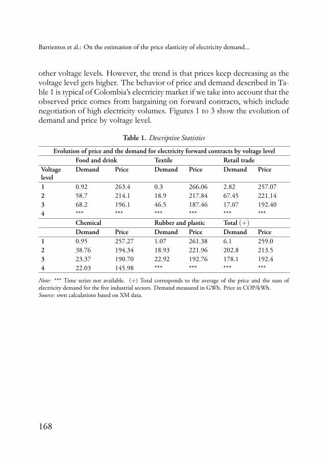
other voltage levels. However, the trend is that prices keep decreasing as thevoltage level gets higher. The behavior of price and demand described in Ta-ble 1 is typical of Colombia’s electricity market if we take into account that theobserved price comes from bargaining on forward contracts, which includenegotiation of high electricity volumes. Figures 1 to 3 show the evolution ofdemand and price by voltage level.

Table 1. Descriptive Statistics

Evolution of price and the demand for electricity forward contracts by voltage levelFood and drink Textile Retail trade

Voltagelevel

Demand Price Demand Price Demand Price

1 0.92 263.4 0.3 266.06 2.82 257.072 58.7 214.1 18.9 217.84 67.45 221.143 68.2 196.1 46.5 187.46 17.07 192.404 *** *** *** *** *** ***

Chemical Rubber and plastic Total (+)

Demand Price Demand Price Demand Price1 0.95 257.27 1.07 261.38 6.1 259.02 38.76 194.34 18.93 221.96 202.8 213.53 23.37 190.70 22.92 192.76 178.1 192.44 22.03 145.98 *** *** *** ***

Note: *** Time series not available. (+) Total corresponds to the average of the price and the sum ofelectricity demand for the five industrial sectors. Demand measured in GWh. Price in COP/kWh.Source: own calculations based on XM data.

168

169

Figure 1.

(a) Demand series for voltage level 1

(b) Price series for voltage level 1

Source: own calculations.



Figure 2.


(b) Price series for voltage level 2


170

171

Figure 3.


(b) Price series for voltage level




III. Empirical results

A. Stationarity Analysis

In order to stablish the stationarity of the data generating process, weperform an augmented Dickey-Fuller test and a Phillips-Perron test as showninMaddala andKim (1988). Table 2 shows the results of the testing procedurefor each series in every voltage level.

Table 2. Phillips-Perron test

Voltage level

Sector (1) (2) (3) (4)

Food and drink Demand I(0) I(0) I(0) ***Price I(0) I(0) I(1) ***

Textile Demand I(1) I(0) I(0) ***Price I(0) I(0) I(1) ***

Chemical Demand I(1) I(0) I(0) I(0)Price I(1) I(1) I(0) I(1)

Rubber and plastic Demand I(0) I(0) I(0) ***Price I(0) I(0) I(1) ***

Retail trade Demand I(1) I(0) I(0) ***Price I(0) I(0) I(0) ***

Total (+) Demand I(0) I(0) I(0) ***Price I(1) I(0) I(1) ***

Note: ***Time series not available. (+) Total corresponds to the average of price and electricity demand inthe five industrial sectors.Source: own calculations based on XM data.

Table 2 shows that in some cases the null hypothesis of a random walkprocess could not be rejected. In these cases, we applied the (1−L) operatorin order to estimate the VAR/SVAR. For instance, series of demand and pricefor the chemical sector at voltage level 1 and price series for the food and drinksector at voltage level 3 have a unit root. It is worth noticing that we cannotfind evidence of a long-run relationship (or co-integrated vectors) between

172

173

the variables. For this, we used the well known methodology developed byEngle and Granger (1987). Statistics tests do not allow us to reject the nullhypothesis of a unit root, so we cannot perform vector correction models(VEC); instead, we use VAR models.

B. Standard VAR and the impulse-response function

We estimate VAR models for every branch of economic activity and ev-ery voltage level. In each case, we include price and demand in the forwardcontract as endogenous variables. Also, we add in a constant, the industrialproduction index and hydrology as exogenous variables. Figures 4 and 5 showthe monthly trends of hydrology and IPI, two typical exogenous variables inthe period under consideration. The data source for hydrology and IPI isXM and National Department of Statitsics (which stands in Spanish for De-partamento Nacional de Estadística or DANE) respectively. It is worth tomention that the residuals produced by all models are stationary processes.

Figure 4. Evolution of monthly hydrology

Note: logarithm of kWh.Source: own development based on XM data.



Figure 5. Evolution of the industrial production index

Source: own development based on DANE data.

The lag-length testing is carried out by performing a likelihood ratio (orLR) test. Results suggest that the optimal lag number to be included in theVAR is between 10 and 12. Thus, we included 12 lags in each regressionbecause we had monthly data. In doing so, we explored and took advantageof all the information contained in the dynamic relationship between demandand price.

As we mentioned above, rigorously speaking, the PED in dynamic andvector models is estimated through the impulse-response function. The IRFsimulates the effect of a rise of 1% in the electricity price on electricity de-mand 12 months ahead. However, our simulations yielded that the IRF is notstatistically significant (see figure 6).

The following graphs illustrate our empirical results, showing the lack ofsignificance of the estimated IRF (solid line) since the upper band is entirelyabove zero and the lower band is below. Similar results are obtained whenthe auto-regressive vectors are estimated by branch of economic activity. Inmany cases, statistically significant lags of prices are obtained; however, theIRF estimate is not significant.

174

175

Figure 6. Impulse-response functions

(a) Impulse variable: price. Response variable: demand. Voltage level 1

(b) Impulse variable: price. Response variable: demand. Voltage level 3




The statistical exercises show that there is not a strong relationship be-tween price and demand in the forward market. This means that long-termelasticities are not detected using the methodology of impulse-response func-tions. Furthermore, the results obtained suggest that the collected data doesnot have the best quality to model the relationship between demand and priceof long-term contracts. In particular, the way in which the prices of contractsand the quantities demanded are reported to the market operator makes itdifficult to identify the data generating process.

C. Structural VAR: short-run approach

We compute IRFs for the SVAR model; however, it yielded disappoint-ing results in terms of statistical significance of the underlying parameters.So, given the discouraging results using IRFs by performing reduced VARas well as SVAR, structural parameters are estimated having as reference thespecification of the model given by (8). We use as endogenous variables theprices/rates and sales/demand by branch of economic activity, and, as exoge-nous variables, again hydrology and IPI are used. The restrictions imposedon each model are given by the matrix

A =

[1 ϕ120 1

], (10)

which explicitly indicates that we are interested in the effect of a change inprice on the demand for electricity. Note that an estimate of the parameterϕ12 with positive sign is interpreted as a negative effect of price on the de-mand for electricity (see equation 8). Table 3 shows the contemporaneous(short-term) elasticities estimated in each model. The critical value of thenormal distribution is in parentheses. It should be around 1.96 or higher tobe considered significant at 5% or less. As in the case of reduced VAR, theresiduals from SVAR are also stationary processes.

The estimated structural parameters show the change in demand for apositive variation in contemporary price of 1%. Note that for voltage level 1,the estimated parameters are significant and with the expected sign (negative)

176

177

for all branches of economic activity, except for the chemical and textile sec-tors. In voltage level 2, the results are consistent and, except for the textilesector, all branches of economic activity show a reduction in demand whenthe price level increases by 1%. The same happens with voltage level 3, exceptfor chemicals. The only sector with an elastic demand is food and beveragesin voltage level 2.

Table 3. Estimated structural parameters

Elasticity of demandBranch of economic activity

Voltage level (1) (2) (3) (4)Food and beverages (FA) −0.5 −3.0 −0.10

(>>2) (>>2) (1.1) ——-Rubber and plastic (RP) −0.72 −0.28 −0.6

(>>2) (>2) (>>2) ——-Chemicals (CH) 0.79 −0.9 0.33 −0.22

(>>2) (>>2) (2.8) ( 2.0)Textiles (T) 0.30 0.06 −0.16

(>>2) 0.6 1.5 ——–Retail Trade (RT) −0.26 −0.19 −0.35

(2.1) (1.6) (>>2) ———Total= AE= FA+RP+CH+T+RT −0.39 −0.92 −0.33

(>>2) (>>2) (>>2) ——–

Note: t values in parenthesis.Source: own calculations.

However, we find that the low response of the quantity demanded, con-sidering a marginal change in price, shows that it would be convenient tomake a seasonal adjustment of forward prices (or in the way in which theinformation is broadcasted).

Conclusions

In this paper, we estimated the PED of forward contracts in the electricitymarket of Colombia considering several economic activities at different volt-



age levels. The study of demand elasticity is important not only to discuss thepossibility of this market to operate competitively, but also because nowadaysthere is a technical debate around the possibility of designing seasonal forwardcontracts in Colombia. Estimating the PED provides valuable informationto market agents in order to construct complete contractual arrangements,especially in the presence of asymmetric information.

In order to compute the PED we described why an SVAR model, andtheir associated matrices, constitute an appropriated framework for its esti-mation. Our main result suggests that some sectors, like food and drink orplastic and rubber manufacturing or even the retail trade sector, are slightlymore sensitive to shocks on prices than the chemical industry or the textilesector. The only economic sector that displays a more elastic demand is foodand drink manufacturing in voltage level 2. However, our general conclusionis that the industrial sectors analyzed show that electricity demand in forwardcontracts is almost inelastic to price variations. This result is consistent withwhat we would expect in an oligopolistic market such as the Colombian one.

The implication of these general results is evident: traders have lots of de-grees of freedom for manipulating contract prices; then, this failure in func-tionality of contract markets gives traders a sort of market power. There-fore, forward contracts in the electricity market of Colombia are in need forchanges, making all information about prices and quantities demanded publicfor all agents. This opens the possibility of investigating and implementingseasonal forward contracts, which may complement the spot market makingColombia’s electricity market more competitive.

References

Agnolucci, Paolo (2009). “The energy demand in the British and German in-dustrial sectors: heterogeneity and common factors”, Energy Economics,Vol. 31, No. 1, pp. 175-187.

Alberini, Anna & Filippini, Massimo (2011). “Response of residential elec-tricity demand to price: the effect of measument error”, Energy Eco-nomics, Vol. 33, No. 5, pp. 889-895.

178

179

Alter, Noel & Syed, Shabid Haider (2011). “An Empirical Analysis of Elec-tricity Demand in Pakistan International”, Journal of Energy Economicsand Policy, Vol. 1, No. 4, pp. 116-139.

Arango, Santiago; Dyner, Isaac & Larsen, Erick (2006). “Lessons fromderegulation: Undertanding electricity markets in South America”, En-ergy Policy, Vol. 14, No. 3, pp. 196-207.

Arzaghi, Mohammad & Squalli, Jay (2015). “How price inelastic is de-mand for gasoline in fuel-subsidizing economies?”, Energy Economics,Vol. 50, pp. 117-124.

Arthur, María de Fátima S.R.; Bond, Craig A. & Wilson, Bryan (2012).“Estimation of elasticities for domestic energy demand in Mozambique”,Energy Economics, Vol. 34, No. 2, pp. 389-409.

Athukorala, Wasantha P.P.A. & Wilson, Clevo (2010). “Estimating shortand long-term residential demand for electricity: New evidence fromShri Lanka”, Energy Economics, Vol. 32, Supplement 1, pp. S34-S40.

Barrientos, Andres Felipe; Olaya, Javier & González, Victor Manuel(2007). “Un modelo Spline para el pronóstico de la demanda de en-ergía eléctrica”, Revista Colombiana de Estadística, Vol. 30, No. 2, pp.187-202.

Beenstock, Michael; Goldin, Epharin & Nabot, Dan (1999). “The de-mand for electricity in Israel”, Energy Economics, Vol. 21, No. 2, pp.168-183.

Bernstein, Mark & Griffin, James (2006). “Regional differences in theprice-elasticity of demand for energy”, Subcontract Report, NREL/SR-620-39512. National Renewable Energy Laboratory.

Bernstein, Ronald & Madlener, Reinhard (2015). “Short- and long-runelectricity demand elasticities at the subsectoral level: a cointegrationanalysis for German manufacturing industries”, Energy Economics, Vol.48, pp. 178-187.



Bose, Ranjan Kumar & Shukla, Megha (1999). “Elasticities of electricitydemand in India”, Energy Policy, Vol. 27, No. 3, pp. 137-146.

Botero, Jesús Alfonso; Castaño, Elkin Argemiro & Vélez, Carlos Eduardo(1990). “Modelo económico de demanda de energía eléctrica en la in-dustria colombiana”, Lecturas de Economía, No. 32-33, pp. 97-124.

Cárdenas, Helena; Vásquez, Felipe & Whittington, Dale (2014). “Amicro data analysis of fuel factors demand, the case of Chileanmanufacturing sector”, Working Paper Series, WP62. Latin Americanand Caribbean Environmental Economics Program. Retrieved from:https://econpapers.repec.org/paper/laewpaper/201462.htm (noviembre22 de 2017).

De Castro, Luciano; Oren, Shmuel; Riascos, Álvaro & Bernal, Miguel(2014). “Transition to centralized unit commitment: An econometricanalysis of Colombia’s experience”, Borradores de Economía, No. 830.Banco de la República, Colombia.

Engle, Robert & Granger, C.W.J. (1987). “Co-integration and error calcu-lation: representaction, estimation and testing”, Ecomometrica, Vol. 55,No. 2, pp. 251-276.

Espinosa, Óscar; Vaca, Paola & Ávila, Raúl (2013). “Elasticidades de de-manda por electricidad e impactos macroeconómicos del precio de laenergia eléctrica em Colombia”, Revista de Métodos Cuantitativos para laEconomía y la Empresa, Vol. 16, pp. 216-249.

Franco, Carlos Jaime; Velázquez, Juan David & Olaya, Yris (2008). “Car-acterización de la demanda mensual de electricidad en Colombina us-ando un modelo de componentes no observable”, Cuadernos de Admin-istración, Vol. 21, No. 36, pp. 221-235.

Halicioglu, Ferda (2007). “Residential electricity demand dynamics inTurkey”, Energy Economics, Vol. 29, pp. 199-210.

Hamilton, James D. (1994). Time Series Analysis. Nueva Jersey: PrincetonUniversity Press.

180

181

Kamerschen, David R. & Porter, David V. (2004). “The demand for res-idential, industrial and total electricity 1973-1998”, Energy Economics,Vol. 26, pp. 87-100.

Labandeira, Xavier; Labeaga, José M.; López-Otero, Xiral (2016). “Ameta-analysis on the price elasticity of energy demand”, Energy Policy,Vol. 102, pp. 549-568.

Labandeira, Xavier; Labeaga, José M. & López-Otero, Xiral (2012), “Es-timation of elasticity price of electricity with incomplete information”,Energy Economics, Vol. 34, No. 3, pp. 627-633.

Lijesen, Mark G., (2007). “The real-time price elasticity of electricity”, EnergyEconomics, Vol. 29, No. 2, pp. 249-258.

Lin, Cynthia C.Y. & Prince, Lea (2013). “Gasoline price volatility and theelasticity of demand for gasoline”, Energy Economics, Vol. 38, pp. 111-117.

Maddala, G.S. & Kim, In-Moo (1998). Unit Roots, Cointegration and Struc-tural Change. New York: Cambridge University Press.

Maddock, Rodney; Castaño, Elkin & Vella, Frank (1992), “EstimatingElectricity Demand: The Cost of Linearising the Budget Constraint”,The Review of Economics and Statistics, Vol. 74 No. 2, pp. 350-354.

Maddock, Rodney & Castaño, Elkin (1991). “The Welfare Impact of RisingBlock Pricing: Electricity in Colombia”, The Energy Journal, Vol. 12, No.4, pp. 65-77.

Maccombie, Charles & Jefferson, Michael (2016). “Renewable and nuclearelectricity: Comparison of environmental impacts”, Energy Policy, Vol.96, pp.758-769.

Narayan, Paresh Kumar & Smyth, Russell (2005). “Electricity consumption,employment and real income in Australia: evidence from multivariateGranger causality tests”, Energy Policy, Vol. 33, No. 9, pp. 1109-1116.



Neto, David (2012). “Testing and estimating time-varying elasticities ofSwiss gasoline demand”, Energy Economics, Vol. 34, No. 6, pp. 1755-1762.

Nienhueser, Ian Andrew & Qiu, Yueming (2016). “Economic and envi-ronmental impacts of providing renewable energy for electric vehiclecharging- A choice experiment study”, Applied Energy, Vol. 180, pp. 256-268.

Ramírez, Gustavo Antionio (1991). “La demanda de energía eléctrica en laindustria colombiana”, Desarrollo y Sociedad, No. 27, pp. 121-139.

Okajima, Shigeharu & Okajima, Hikoro (2013). “Estimation of Japaneseprice elasticities of residential electricity demand, 1990-2007”, EnergyEconomics, Vol. 40, pp. 433-440.

Polemis, Michael L. (2007). “Modeling industrial energy demand in Greeceusing cointegration techniques”, Energy Policy, Vol. 35, No. 8, pp. 4039-4050.

Pollitt, Michael (2009). “Evaluating the evidence on electricity reform:Lessons for the South East Europe (SEE) market”, Utilities Policy, Vol.17, No. 1, 13-23.

Thimmapuram, Prakash, R. & Kim, Jinho (2013). “Consumers price elas-ticity of demand modeling with economic effects on electricity marketsusing an agent-based model”, IEEE Transactions on Smart Grid, Vol. 14,No. 1, pp. 390-397.

Ziramba, Emmanuel (2008). “The demand for residential electricity in SouthAfrica”, Energy Policy, Vol. 36, No. 9, pp. 3460-3466.

182

on the estimation of the price elasticity of electricity ... · jorge barrientos, esteban velilla,...

Documents