on the global solution of linear programs with linear ... · on the global solution of linear...
TRANSCRIPT

On the Global Solution of Linear Programs with Linear
Complementarity Constraints∗†
Jing Hu, John E. Mitchell, Jong-Shi Pang, Kristin P. Bennett, and Gautam Kunapuli
March 7, 2007
Abstract
This paper presents a parameter-free integer-programming based algorithm for the global resolutionof a linear program with linear complementarity constraints (LPEC). The cornerstone of the algorithmis a minimax integer program formulation that characterizes and provides certificates for the threeoutcomes—infeasibility, unboundedness, or solvability—of an LPEC. An extreme point/ray generationscheme in the spirit of Benders decomposition is developed, from which valid inequalities in the formof satisfiability constraints are obtained. The feasibility problem of these inequalities and the carefullyguided linear programming relaxations of the LPEC are the workhorse of the algorithm, which alsoemploys a specialized procedure for the sparsification of the satifiability cuts. We establish the finitetermination of the algorithm and report computational results using the algorithm for solving randomlygenerated LPECs of reasonable sizes. The results establish that the algorithm can handle infeasible,unbounded, and solvable LPECs effectively.
1 Introduction
Forming a subclass of mathematical programs with equilibrium constraints (MPECs) [33, 35, 11], linearprograms with linear complementarity constraints (LPECs) are disjunctive linear optimization problemsthat contain a set of complementarity conditions. In turn, a large subclass of LPECs are bilevel lin-ear/quadratic programs [10] that recently have been proposed as a modeling framework for parametercalibration in a host of machine learning applications [6, 29, 28]. While there have been significantrecent advances on nonlinear programming (NLP) based computational methods for solving MPECs,[1, 2, 3, 8, 14, 15, 18, 19, 25, 26, 21, 31, 32, 40, 41], much of which have nevertheless focused on obtainingstationary solutions [12, 13, 33, 35, 34, 36, 40, 46, 45, 44], the global solution of an LPEC remains elu-sive. Particularly impressive among these advances is the suite of NLP solvers publicly available on theneos system at http://www-neos.mcs.anl.gov/neos/solvers/index.html; many of them, such as filter,are capable of producing a solution of some sort to an LPEC very efficiently. Yet, they are incapable ofascertaining the quality of the computed solution. This is the major deficiency of these numerical solvers.Continuing our foray into the subject of computing global solutions of LPECs, which begins with therecent article [38] that pertains to a special problem arising from the optimization of the value-at-risk, thepresent paper proposes a parameter-free integer-programming based cutting-plane algorithm for globallyresolving a general LPEC.
As a disjunctive linear optimization problem, the global solution of an LPEC has been the subject ofsustained, but not particularly focused investigation since the early work of Ibaraki [22, 23] and Jeroslow
∗This work was supported in part by the Office of Naval Research under grant no. N00014-06-1-0014. The work ofMitchell was supported by the National Science Foundation under grant DMS-0317323.
†All authors are with the Department of Mathematical Sciences, Rensselaer Polytechnic Institute, Troy, New York 12180-1590, U.S.A. Email addresses: huj, mitchj, pangj, bennek, [email protected].
1

[24], who pioneered some cutting-plane methods for solving a “complementary program”, which is ahistorical and not widely used name for an LPEC. Over the years, various integer programming basedmethods [4, 5, 20] and global optimization based methods [16, 17, 42, 43] have been developed that areapplicable to an LPEC. In this paper, we present a new cutting-plane method that will successfully resolvea general LPEC in finite time; i.e., the method will terminate with one of the following three mutuallyexclusive conclusions: the LPEC is infeasible, the LPEC is feasible but has an unbounded objective, orthe LPEC attains a finite optimal solution. We also leverage the advances of the NLP solvers and useone of them to benchmark our algorithm. In addition, we propose a simple linear programming basedpre-processor whose effectiveness will be demonstrated via computational results.
The proposed method begins with an equivalent formulation of an LPEC as a 0-1 integer program(IP) involving a conceptually very large parameter, whose existence is not guaranteed unless a certainboundedness condition holds. Via dualization of the linear programming relaxation of the IP, we obtaina minimax 0-1 integer program, which yields a certificate for the three states of the LPEC, withoutany a priori boundedness assumption. The original 0-1 IP with the conceptual parameter providesthe formulation for the application of Benders decomposition [30], which we show can be implementedwithout involving the parameter in any way. Thus, the resulting algorithm is reminiscent of the well-known Phase I implementation of the “big-M” method for solving linear programs, wherein the big-Mformulation is only conceptual whose practical solution does not require the knowledge of the scalar M.
The implementation of our parameter-free algorithm is accomplished by solving integer subprogramsdefined solely by satisfiability constraints [7, 27]; in turn, each such constraint corresponds to a “piece”of the LPEC. Using this interpretation, the overall algorithm can be considered as solving the LPECby searching on its (finitely many) linear programming pieces, with the search guided by solving thesatisfiability IPs. The implementation of the algorithm is aided by valid upper bounds on the LPECoptimal objective value that are being updated as the algorithm progresses, which also serve to providethe desired certificates at the termination of the algorithm.
The organization of the rest of the paper is as follows. Section 2 presents the formal statement ofthe LPEC, summarizes the three states of the LPEC, and introduces the new minmax IP formulation.Section 3 reformulates the minmax IP formulation in terms of the extreme points and rays of the keypolyhedron Ξ (see (6)) and established the theoretical foundation for the cutting-plane algorithm to bepresented in Section 5. The key steps of the algorithm, which involve solving linear programs (LPs) tosparsify the satisfiability constraints, are explained in Section 4. The sixth and last section reports thecomputational results and completes the paper with some concluding remarks.
2 Preliminary Discussion
Let c ∈ <n, d ∈ <m, f ∈ <k, q ∈ <m, A ∈ <k×m, B ∈ <k×m, M ∈ <m×m, and N ∈ <m×n begiven. Consider the linear program with linear complementarity constraints (LPEC) [37] of finding(x, y) ∈ <n ×<m in order to
minimize(x,y)
cT x + dT y
subject to Ax + By ≥ f
and 0 ≤ y ⊥ q + Nx + My ≥ 0,
(1)
where a ⊥ b means that the two vectors are orthogonal; i.e., aT b = 0. It is well-known that the LPECis equivalent to the minimization of a large number of linear programs, each defined on one piece ofthe feasible region of the LPEC. That is, for each subset α of {1, · · · ,m} with complement α, we may
2
consider the LP(α):minimize
(x,y)cT x + dT y
subject to Ax + By ≥ f
( q + Nx + My )α ≥ 0 = yα
and ( q + Nx + My )α = 0 ≤ yα.
(2)
The following facts are obvious:
(a) the LPEC (1) is infeasible if and only if the LP(α) is infeasible for all α ⊆ {1, · · · ,m};
(b) the LPEC (1) is feasible and has an unbounded objective if and only if the LP(α) is feasible and hasan unbounded objective for some α ⊆ {1, · · · ,m};
(c) the LPEC (1) is feasible and attains a finite optimal objective value if and only if (i) a subset α of{1, · · · ,m} exists such that the LP(α) is feasible, and (b) every such feasible LP(α) has a finiteoptimal objective value; in this case, the optimal objective value of the LPEC (1), denoted LPECmin,is the minimum of the optimal objective values of all such feasible LPs.
The first step in our development of an IP-based algorithm for solving the LPEC (1) without any apriori assumption is to derive results parallel to the above three facts in terms of some parameter-freeinteger problems. For this purpose, we recall the standard approach of solving (1) as an IP containing alarge parameter. This approach is based on the following “equivalent” IP formulation of (1) wherein thecomplementarity constraint is reformulated in terms of the binary vector z ∈ {0, 1}m via a conceptuallyvery large scalar θ > 0:
minimize(x,y,z)
cT x + dT y
subject to Ax + By ≥ f
θ z ≥ q + Nx + My ≥ 0
θ(1− z ) ≥ y ≥ 0
and z ∈ { 0, 1 }m,
(3)
where 1 is the m-vector of all ones. In the standard approach, we first derive a valid value on θ bysolving LPs to obtain bounds on all the variables and constraints of (1). We then solve the fixed IP(3) using the so-obtained θ by, for example, the Benders approach. There are two obvious drawbacks ofsuch an approach: one is the limitation of the approach to problems with bounded feasible regions; theother drawback is the nontrivial computation to derive the required bounds even if they are known toexist implicitly. In contrast, our new approach removes such a theoretical restriction and eliminates thefront-end computation of bounds. The price of the new approach is that it solves a (finite) family of IPsof a special type, each defined solely by constraints of the satisfiability type. The following discussionsets the stage for the approach.
For a given binary vector z and a positive scalar θ, we associate with (3) the linear program below,which we denote LP(θ; z):
minimize(x,y)
cT x + dT y
subject to Ax + By ≥ f ( λ )
Nx + My ≥ −q ( u− )
−Nx−My ≥ q − θ z ( u+ )
−y ≥ −θ (1− z ) ( v )
and y ≥ 0,
(4)
3

where the dual variables of the respective constraints are given in the parentheses. The dual of (4), whichwe denote DLP(θ, z), is:
maximize(λ,u±,v)
fT λ + qT ( u+ − u− )− θ[zT u+ + (1− z )T v
]subject to AT λ−NT ( u+ − u− ) = c
BT λ−MT ( u+ − u− )− v ≤ d
and ( λ, u±, v ) ≥ 0.
(5)
Let Ξ ⊆ <k+3m be the feasible region of the DLP(θ, z); i.e.,
Ξ ≡
{( λ, u±, v ) ≥ 0 : AT λ−NT ( u+ − u− ) = c
BT λ−MT ( u+ − u− )− v ≤ d
}. (6)
Note that Ξ is a fixed polyhedron independent of the pair (θ, z); Ξ has at least one extreme point ifit is nonempty. Let LPmin(θ; z) and d(θ; z) denote the optimal objective value of (4) and (5), respec-tively. Throughout, we adopt the standard convention that the optimal objective value of an infeasiblemaximization (minimization) problem is defined to be −∞ (∞, respectively). We summarize some basicrelations between the above programs in the following elementary result.
Proposition 1. The following three statements hold.
(a) Any feasible solution (x0, y0) of (1) induces a pair (θ0, z0), where θ0 > 0 and z0 ∈ {0, 1}m, such that
the tuple (x0, y0, z0) is feasible to (3) for all θ ≥ θ0; such a z0 has the property that
( q + Nx0 + My0 )i > 0 ⇒ z0i = 1
( y0 )i > 0 ⇒ z0i = 0.
(7)
(b) Conversely, if (x0, y0, z0) is feasible to (3) for some θ ≥ 0, then (x0, y0) is feasible to (1).
(c) If (x0, y0) is an optimal solution to (1), then it is optimal to the LP(θ, z0) for all pairs (θ, z0) suchthat θ ≥ θ0 and z0 satisfies (7); moreover, for each θ > θ0, any optimal solution (λ, u±, v) of theDLP(θ, z0) satisfies (z0)T u+ + (1− z0 )T v = 0.
Proof. Only (c) requires a proof. Suppose (x0, y0) is optimal to (1). Let (θ, z0) such that θ ≥ θ0 andz0 ∈ {0, 1}m satisfies (7). Then (x0, y0) is feasible to the LP(θ, z0); hence
cT x0 + dT y0 ≥ LPmin(θ, z0). (8)
But the reverse inequality must hold because of (b) and the optimality of (x0, y0) to (1). Consequently,equality holds in (8). For θ > θ0, if i is such that z0
i > 0, then
( q + Nx0 + My0 ) ≤ θ0 z0i < θ z0
i ,
and complementary slackness implies (u+)i = 0. Similarly, we can show that z0i = 0⇒ vi = 0. Hence (c)
follows. �
4
2.1 The parameter-free dual programs
Property (c) of Proposition 1 suggests that the inequality constraint zT u++(1−z)T v ≤ 0, or equivalently,the equality constraint zT u+ + (1 − z)T v = 0 (because all variables are nonnegative and z ∈ {0, 1}m),should have an important role to play in an IP approach to the LPEC. This motivates us to define twovalue functions on the binary vectors. Specifically, for any z ∈ {0, 1}m, define
< ∪ {±∞} 3 ϕ(z) ≡ maximum(λ,u±,v)
fT λ + qT ( u+ − u− )
subject to AT λ−NT ( u+ − u− ) = c
BT λ−MT ( u+ − u− )− v ≤ d
( λ, u±, v ) ≥ 0
and zT u+ + (1− z)T v ≤ 0
(9)
and its homogenization:
{ 0,∞} 3 ϕ0(z) ≡ maximum(λ,u±,v)
fT λ + qT ( u+ − u− )
subject to AT λ−NT ( u+ − u− ) = 0
BT λ−MT ( u+ − u− )− v ≤ 0
( λ, u±, v ) ≥ 0
and zT u+ + (1− z )T v ≤ 0.
(10)
Clearly, (10) is always feasible and ϕ0(z) takes on the values 0 or∞ only. Unlike (10) which is independentof the pair (c, d), (9) depends on (c, d) and is not guaranteed to be feasible; thus ϕ(z) ∈ < ∪ {±∞}. Forany pair (c, d) for which (9) is feasible, we have
ϕ(z) < ∞ ⇔ ϕ0(z) = 0.
To this equivalence we add the following proposition that describes a one-to-one correspondence between(10) and the feasible pieces of the LPEC. The support of a vector z, denoted supp(z) is the index set ofthe nonzero components of z.
Proposition 2. For any z ∈ {0, 1}m, ϕ0(z) = 0 if and only if the LP(α) is feasible, where α ≡ supp(z).
Proof. The dual of (10) is
minimize(x,y)
0T x + 0T y
subject to Ax + By ≥ f
θ z ≥ q + Nx + My ≥ 0
and θ (1− z ) ≥ y ≥ 0.
(11)
By LP duality, it follows that if ϕ0(z) = 0, then (11) is feasible for any θ > 0; conversely, if (11) is feasiblefor some θ > 0, then ϕ0(z) = 0. In turn, it is easy to see (11) is feasible for some θ > 0 if and only if theLP(α) is feasible for α ≡ supp(z). �
For subsequent purposes, it would be useful to record the following equivalence between the extremepoints/rays of the feasible region of (9) and those of the feasible set Ξ.
Proposition 3. For any z ∈ [0, 1]m, a feasible solution (λp, u±,p, vp) of (9) is an extreme point in thisregion if and only if it is extreme in Ξ; a feasible ray (λr, u±,r, vr) of (9) is extreme in this region if andonly if it is extreme in Ξ.
5
Proof. We prove only the first assertion; that for the second is similar. The sufficiency is obvious. Toprove the converse, suppose that (λp, u±,p, vp) is an extreme solution of (9). Then this triple must bean element of Ξ. If it lies on the line segment of two other feasible solutions of Ξ, then the latter twosolutions must satisfy the additional constraint zT u+ + (1 − z)T v ≤ 0. Therefore, (λp, u±,p, vp) is alsoextreme in Ξ. �
2.2 The set Z and a minimax formulation
We now define the key set of binary vectors:
Z ≡ { z ∈ { 0, 1 }m : ϕ0(z) = 0 } ,
which, by Proposition 2, is the feasibility descriptor of the feasible region of the LPEC (1). Note that Zis a finite set. We also define the minimax integer program:
minimizez∈Z
ϕ(z) ≡
maximum(λ,u±,v)
fT λ + qT ( u+ − u− )
subject to AT λ−NT ( u+ − u− ) = c
BT λ−MT ( u+ − u− )− v ≤ d
( λ, u±, v ) ≥ 0
and zT u+ + (1− z)T v ≤ 0.
(12)
Since Z is a finite set, and since ϕ(z) ∈ <∪ {−∞} for z ∈ Z, it follows that argminz∈Z
ϕ(z) 6= ∅ if and only
if Z 6= ∅. The following result rephrases the three basic facts connecting the LPEC (1) and its LP piecesin terms of the IP (12).
Theorem 4. The following three statements hold:
(a) the LPEC (1) is infeasible if and only if minz∈Z
ϕ(z) =∞ (i.e., Z = ∅);
(b) the LPEC (1) is feasible and has an unbounded objective value if and only if minz∈Z
ϕ(z) = −∞ (i.e.,
z ∈ Z exists such that ϕ(z) = −∞);
(c) the LPEC (1) attains a finite optimal objective value if and only if −∞ < minz∈Z
ϕ(z) <∞.
In all cases, LPECmin = minz∈Z
ϕ(z); moreover, for any z ∈ {0, 1}m for which ϕ(z) > −∞, LPECmin ≤ ϕ(z).
Proof. Statement (a) is an immediate consequence of Proposition 2. Statement (b) is equivalent tosaying that the LPEC (1) is feasible and has an unbounded objective if and only if z ∈ {0, 1}m existssuch that ϕ0(z) = 0 and ϕ(z) = −∞. Suppose that the LPEC (1) is feasible and unbounded. Then anindex set α ⊆ {1, · · · ,m} exists such that the LP(α) is feasible and unbounded. Letting z ∈ {0, 1}m besuch that supp(z) = α and α be the complement of α in {1, · · · ,m}, we have ϕ0(z) = 0. Moreover, thedual of the (unbounded) LP(α) is
maximize(λ,uα,u−α )
fT λ + ( qα )T uα − ( qα )T u−α
subject to AT λ− ( Nα• )T uα + ( Nα• )T u−α = c
( B•α )T λ− ( Mαα )T uα + ( Mαα )T u−α ≤ dα
and (λ, u−α ) ≥ 0,
(13)
6
which is equivalent to the problem (9) corresponding to the binary vector z defined here. (Note, the •in the subscripts is the standard notation in linear programming, denoting rows/columns of matrices.)Therefore, since (13) is infeasible, it follows that ϕ(z) = −∞ by convention. Conversely, suppose thatz ∈ {0, 1}m exists such that ϕ0(z) = 0 and ϕ(z) = −∞. Let α ≡ supp(z) and α ≡ complement of αin {1, · · · ,m}. It then follows that (11), and thus the LP(α), is feasible. Moreover, since ϕ(z) = −∞,it follows that (13), being equivalent to (9), is infeasible; thus the LP(α) is unbounded. Statement (c)follows readily from (a) and (b). The equality between LPECmin and min
z∈Zϕ(z) is due to the fact that the
maximizing LP defining ϕ(z) is essentially the dual of the piece LP(α). To prove the last assertion ofthe theorem, let z ∈ {0, 1}m be such that ϕ(z) > −∞. Without loss of generality, we may assume thatϕ(z) <∞. Thus the LP (9) attains a finite maximum; hence ϕ0(z) = 0. Therefore z ∈ Z and the boundLPECmin ≤ ϕ(z) holds readily. �
3 The Benders Approach
In essence, our strategy for solving the LPEC (1) is to apply a Benders approach to the minimax IP(12). For this purpose, we let
{ (λp,i, u±,p,i, vp,i
) }K
i=1and
{ (λr,j , u±,r,j , vr,j
) }L
j=1be the finite set of
extreme points and extreme rays of the polyhedron Ξ. Note that K ≥ 1 if and only if Ξ 6= ∅. (Theseextreme points and rays will be generated as needed. For the discussion in this section, we take them asavailable.) In what follows, we derive a restatement of Theorem 4 in terms of these extreme points andrays.
The IP (12) can be written as:
minimizez∈Z
maximum( ρp, ρr )≥0
K∑i=1
ρpi
[fT λp,i + qT (u+,p,i − u−,p,i)
]+
L∑j=1
ρrj
[fT λr,j + qT (u+,r,j − u−,r,j)
]
subject toK∑
i=1
ρpi
[zT u+,p,i + (1− z)T vp,i
]+
L∑j=1
ρrj
[zT u+,r,j + (1− z)T vr,j
]≤ 0
andK∑
i=1
ρpi = 1,
(14)
which is the master IP. It turns out that the set Z can be completely described in terms of certain raycuts, whose definition requires the index set:
L ≡{
j ∈ { 1, · · · , L } : fT λr,j + qT (u+,r,j − u−,r,j) > 0}
.
The following proposition shows that the set Z can be described in terms of satisfiability inequalitiesusing the extreme rays in L.
Proposition 5. Z =
z ∈ {0, 1}m :∑
`:u+,r,j` >0
z` +∑
`:vr,j` >0
( 1− z` ) ≥ 1, ∀ j ∈ L
.
Proof. This is obvious because ϕ0(z) is equal to
maximizeρr≥0
L∑j=1
ρrj
[fT λr,j + qT ( u+,r,j − u−,r,j )
]
subject toL∑
j=1
ρrj
[zT u+,r,j + (1− z)T vr,j
]≤ 0
7
and the latter maximization problem has a finite optimal solution if and only if
fT λr,j + qT ( u+,r,j − u−,r,j ) > 0 =⇒ zT u+,r,j + (1− z)T vr,j > 0
⇐⇒∑
`:u+,r,j` >0
z` +∑
`:vr,j` >0
( 1− z` ) ≥ 1.
Therefore, the equality between Z and the right-hand set is immediate. �
An immediate corollary of Proposition 5 is that it provides a certificate of infeasibility for the LPEC.
Corollary 6. If R ⊆ L exists such that z ∈ {0, 1}m :∑
`:u+,r,j` >0
z` +∑
`:vr,j` >0
( 1− z` ) ≥ 1, ∀ j ∈ R
= ∅,
then the LPEC (1) is infeasible.
Proof. The assumption implies that Z = ∅. Thus the infeasibility of the LPEC follows from Theo-rem 4(a). �
In view of Proposition 5, (14) is equivalent to:
minimizez∈Z
maximumρp≥0
K∑i=1
ρpi
[fT λp,i + qT (u+,p,i − u−,p,i)
]
subject toK∑
i=1
ρpi
[zT u+,p,i + (1− z)T vp,i
]≤ 0
andK∑
i=1
ρpi = 1,
. (15)
Note that the LPECmin is equal to the minimum objective value of (15). Similar to the inequality:∑`:u+,r,j
` >0
z` +∑
`:vr,j` >0
( 1− z` ) ≥ 1,
which we call a ray cut (because it is induced by an extreme ray), we will make use of a point cut:∑`:u+,p,i
` >0
z` +∑
`:vp,i` >0
( 1− z` ) ≥ 1,
that is induced by an extreme point (λp,i, u±,p,i, vp,i) of Ξ chosen from the following collection:
K ≡{
i ∈ { 1, · · · ,K } : fT λp,i + qT ( u+,p,i − u−,p,i ) = ϕ(z) for some z ∈ Z}
.
Note that K 6= ∅ ⇒ Z 6= ∅, which in turn implies that the LPEC (1) is feasible. Moreover,
mini∈K
[fT λp,i + qT ( u+,p,i − u−,p,i )
]≥ LPECmin.
8
For a given pair of subsets P ×R ⊆ K × L, let
Z(P,R) ≡
z ∈ { 0, 1 }m :
∑`:u+,r,j
` >0
z` +∑
`:vr,j` >0
( 1− z` ) ≥ 1, ∀ j ∈ R
∑`:u+,p,i
` >0
z` +∑
`:vp,i` >0
( 1− z` ) ≥ 1, ∀ i ∈ P
.
We have the following result.
Proposition 7. If there exists P ×R ⊆ K × L such that
mini∈P
[fT λp,i + qT ( u+,p,i − u−,p,i )
]> LPECmin,
then argminz∈Z
ϕ(z) ⊆ Z(P,R).
Proof. Let z ∈ Z be a minimizer of ϕ(z) on Z. (The proposition is clearly valid if no such minimizerexists.) If z 6∈ Z(P,R), then there exists i ∈ P such that∑
`:u+,p,i` >0
z` +∑
`:vp,i` >0
( 1− z` ) = 0.
Hence, (λp,i, u±,p,i, vp,i) is feasible to the LP (9) corresponding to ϕ(z); thus
LPECmin = ϕ(z) ≥ fT λp,i + qT (u+,p,i − u−,p,i) > LPECmin,
which is a contradiction. �
Analogous to Corollary 6, we have the following corollary of Proposition 7.
Corollary 8. If there exists P ×R ⊆ K × L with P 6= ∅ such that Z(P,R) = ∅, then
LPECmin = mini∈P
[fT λp,i + qT ( u+,p,i − u−,p,i )
]∈ (−∞,∞ ). (16)
Proof. Indeed, if the claimed equality does not hold, then argminz∈Z
ϕ(z) = ∅. But this implies Z = ∅,
which contradicts the assumption that P 6= ∅. �
Combining Corollaries 6 and 8, we obtain the desired restatement of Theorem 4 in terms of theextreme points and rays of Ξ.
Theorem 9. The following three statements hold:
(a) the LPEC (1) is infeasible if and only if a subset R ⊆ L exists such that Z(∅,R) = ∅;
(b) the LPEC (1) is feasible and has an unbounded objective if and only if Z(K,L) 6= ∅;
(c) the LPEC (1) attains a finite optimal objective value if and only if a pair P ×R ⊆ K×L exists withP 6= ∅ such that Z(P,R) = ∅.
Proof. Statement (a) follows easily from Corollary 6 by noting that a subset R ⊆ L exists such thatZ(∅,R) = ∅ if and only if Z = Z(∅,L) = ∅. To prove (b), suppose first Z(K,L) 6= ∅. Let z ∈ Z(K,L).Then z ∈ Z. We claim that ϕ(z) = −∞; i.e., the LP (9) corresponding to z is infeasible. Assumeotherwise, then since ϕ0(z) = 0, it follows that ϕ(z) is finite. Hence there exists an extreme point
9

(λp,i, u±,p,i, vp,i) of the LP (9) corresponding to z such that fT λp,i + qT (u+,p,i − u−,p,i) = ϕ(z); thus theindex i ∈ K, which implies ∑
`:u+,p,i` >0
z` +∑
`:vp,i` >0
( 1− z` ) ≥ 1,
because z ∈ Z(K,L). But this contradicts the feasibility of (λp,i, u±,p,i, vp,i) to the LP (9) correspondingto z. Therefore, the LPEC (1) is feasible and has an unbounded objective value; thus, the “if” statementin (b) holds. Conversely, suppose LPECmin = −∞. By Theorem 4, it follows that z ∈ Z exists such thatϕ(z) = −∞; i.e., the LP (9) corresponding to z is infeasible. In turn, this means that
z T u+,p,i + (1− z )T vp,i > 0
for all i = 1, · · · ,K; or equivalently, ∑`:u+,p,i
` >0
z` +∑
`:vp,i` >0
( 1− z` ) ≥ 1,
for all i = 1, · · · ,K. Consequently, z ∈ Z(K,L). Hence, statement (b) holds. Finally, the “if” statementin (c) follows from Corollary 8. Conversely, if the LPEC (1) has a finite optimal solution, then by (b),it follows that Z(K,L) = ∅. Since the LPEC (1) is feasible, K 6= ∅ by (a), establishing the “only if”statement in (c). �
Theorem 9 constitutes the theoretical basis for the algorithm to be presented in Section 5 for resolvingthe LPEC. Through the successive generation of extreme points and rays of Ξ, the algorithm searchesfor a pair of subsets P ×R such that Z(P,R) = ∅. If such a pair can be successfully identified, then theLPEC is either infeasible (P = ∅) or attains a finite optimal solution (P 6= ∅). If no such pair is found,then the LPEC is unbounded. In the algorithm, the last case is identified with a binary vector z ∈ Zwith ϕ(z) = −∞, i.e., the LP (9) is infeasible. Based on the value function ϕ(z) and the point/ray cuts,the algorithm will be shown to terminate in finite time.
4 Simple Cuts and Sparsification
In this section, we explain several key steps in the main algorithm to be presented in the next section.The first idea is a version of the well-known Gomory cut in integer programming specialized to the LPECand which has previously been employed for bilevel LPs; see [5]; the second idea aims at “sparsifying”the ray/point cuts to facilitate the computation of elements of the working sets Z(P,R). Specifically, asatisfiability constraint:∑
i∈I ′zi +
∑j∈J ′
( 1− zj ) ≥ 1 is sparser than∑i∈I
zi +∑j∈J
( 1− zj ) ≥ 1
if I ′ ⊆ I and J ′ ⊆ J . In general, a satisfiability inequality cuts off certain LP pieces of the LPEC;the sparser the inequality is the more pieces it cuts off. Thus, it is desirable to sparsify a cut as muchas possible. Nevertheless, sparsification requires the solution of linear subprograms; thus one needs tobalance the work required with the benefit of the process.
10
4.1 Simple cuts
The following discussion is a minor variant of that presented in [5] for bilevel LPs. Consider the LPrelaxation of the LPEC (1):
minimize(x,y)
cT x + dT y
subject to Ax + By ≥ f
and 0 ≤ y, w ≡ q + Nx + My ≥ 0,
(17)
where the orthogonal condition yT w = 0 is dropped. Assume that by solving this LP, an optimal solutionis obtained that fails the latter orthogonality condition, say yiwi > 0 in this solution. A basic solution ofthe LP provides an expression of wi and yi as follows:
wi = wi0 −∑
sj :nonbasicaj sj and yi = yi0 −
∑sj :nonbasic
bj sj
with min(wi0, yi0) > 0. It is not difficult to show that the following inequality must be satisfied by allfeasible solutions of the LPEC (1) ∑
sj : nonbasicmax(aj ,bj)>0
max(
aj
wi0,
bj
yi0
)sj ≥ 1 (18)
Note that if aj ≤ 0 for all nonbasic j, then wi > 0 = yi for every feasible solution of the LPEC (1). Asimilar remark can be made if bj ≤ 0 for all nonbasic j.
Following the terminology in [5], we call the inequality (18) a simple cut. Multiple such cuts can beadded to the constraint Ax + By ≥ f , resulting in a modified inequality Ax + By ≥ f . We can generateand add even more simple cuts by repeating the above step. This strategy turns out to be a very effectivepre-processor for the algorithm to be described in the next section. At the end of this pre-processor, weobtain an optimal solution (x, y, w) of (17) that remains infeasible to the LPEC (otherwise, this solutionwould be optimal for the LPEC); the optimal objective value cT x + dT y provides a valid lower boundfor LPECmin. (Note: if (17) is unbounded, then the pre-processor does not produce any cuts or a finitelower bound.)
LPEC feasibility recovery
Occurring in many applications of the LPEC, the special case B = 0 deserves a bit more discussion. Firstnote that in this case, the modified matrix B is not necessarily zero. Nevertheless, the solution (x, y, w)obtained from the simple-cut pre-processor can be used to produce a feasible solution to the LPEC (1)by simply solving the linear complementarity problem (LCP): 0 ≤ y ⊥ q + Nx + My ≥ 0 (assumingthat the matrix M has favorable properties so that this step is effective). Letting y ′ be a solution tothe latter LCP, the objective value cT x + dT y ′ yields a valid upper bound to LPECmin. This recoveryprocedure of an LPEC feasible solution can be extended to the case where B 6= 0. (Incidentally, this classof LPECs is generally “more difficult” than the class where B = 0, where the difficulty is determined byour empirical experience from the computational tests.) Indeed, from any feasible solution (x, y, w) tothe LP relaxation of the LPEC (1) but not to the LPEC itself, we could attempt to recover a feasiblesolution to the LPEC along with an element in Z by either solving the LP(α), where α ≡ {i : yi ≤ wi},or by solving ϕ(z), where zα = 1 and zα = 0. A feasible solution to this LP piece yields a feasible solutionto the LPEC and a finite upper bound. In general, there is no guarantee that this procedure will alwaysbe successful; nevertheless, it is very effective when it works.
11
4.2 Cut management
A key step in our algorithm involves the selection of elements in the sets Z(P,R) for various index pairs(P,R). Generally speaking, this involves solving integer subprograms. Recognizing that the constraintsin each Z(P,R) are of the satisfiability type, we could in principle employ special algorithms for imple-menting this step (see [7, 27] and the references therein for some such algorithms). To facilitate suchselection, we have developed a special heuristic that utilizes a valid upper bound of LPECmin to sparsifythe terms in the ray/point cuts in a working set. In what follows, we describe how the algorithm managesthese cuts.
There are three pools of cuts, labeled Zwork–the working pool, Zwait–the wait pool, and Zcand–thecandidate pool. Inequalities in Zwork are valid sparsifications of those in Z(P,R) corresponding to acurrent pair (P,R). Thus, the set of binary vectors satisfying the inequalities in Zwork, which we denoteZwork, is a subset of Z(P,R). Inequalities in Zcand are candidates for sparsification; the sparsificationprocedure described below always ends with this set empty. The decision of whether or not to sparsifya valid inequality is made according to a current LPEC upper bound and a small scalar δ > 0. Inessence, the sparsification is an effective way to facilitate the search for a feasible element in Zwork. Atone extreme, a sparsest inequality with only one term in it automatically fixes one complementarity;e.g., z1 ≥ 1 fixes w1 = 0; at another extreme, it is computationally more difficult to find feasible pointssatisfying many dense inequalities.
We sparsify an inequality ∑i∈I
zi +∑j∈J
( 1− zj ) ≥ 1 (19)
in the following way. Let I = I1 ∪ I2 be a partition of I into two disjoint subsets I1 and I2; similarly,let J = J1 ∪ J2. We split (19), which we call the parent, into two sub-inequalities:∑
i∈I1
zi +∑j∈J1
( 1− zj ) ≥ 1 and∑i∈I1
zi +∑j∈J2
( 1− zj ) ≥ 1; (20)
and test both to see if they are valid for the LPEC. To test the left-hand inequality, we consider the LPrelaxation (17) of the LPEC (1) with the additional constraints wi = (q + Nx + My)i = 0 for i ∈ I1and yi = 0 for i ∈ J1, which we call a relaxed LP with restriction. If this LP has an objective valuegreater than the current LPECub, then we have successfully sparsified the inequality (19) into the sparserinequality: ∑
i∈I1
zi +∑j∈J1
( 1− zj ) ≥ 1, (21)
which must be valid for the LPEC. Otherwise, using the feasible solution to the relaxed LP, we employthe LPEC feasibility recovery procedure to compute an LPEC feasible solution along with a binary z ∈ Z.If successful, one of two cases happen: if ϕ(z) ≥ LPECub, then a new cut can be generated; otherwise,we have reduced the LPEC upper bound. Either case, we obtain positive progress in the algorithm.If no LPEC feasible solution is recovered, then we save the cut (21) in the wait pool Zwait for laterconsideration. In essence, cuts in the wait pool are not yet proven to be valid for the LPEC; they will berevisited when there is a reduction in LPECub. Note that every inequality in Zwait has an LP optimalobjective value associated with it that is less than the current LPEC upper bound.
In our experiment, we randomly divide the sets I and J roughly into two equal halves each and adopta strategy that attempts to sparsify the root inequality (19) as much as possible via a random branchingrule. The following illustrates one such division:
z1 + z3 + z4 + (1− z2) + (1− z6) ≥ 1↙ ↘
z1 + z3 + (1− z2) ≥ 1 z4 + (1− z6) ≥ 1.
12
We use a small scalar δ > 0 to help decide on the subsequent branching. In essence, we only branch ifthe inequality appears strong. Solving LPs, the procedure below sparsifies a given valid inequality forthe LPEC, called the root of the procedure.
Sparsification procedure. Let (19) be the root inequality to be sparsified, LPECub be the currentLPEC upper bound, and δ > 0 be a given scalar. Branch (19) into two sub-inequalities (20), both ofwhich we put in the set Zcand.
Main step. If Zcand is empty, terminate. Otherwise pick a candidate inequality in Zcand, say the leftone in (20) with the corresponding pair of index sets (I1,J1). Solve the LP relaxation (17) of theLPEC (1) with the additional constraints wi = (q + Nx + My)i = 0 for i ∈ I1 and yi = 0 for i ∈ J1,obtaining an LP optimal objective value, say LPrlx ∈ < ∪ {±∞}. We have the following three cases.
• If LPrlx ∈ [ LPECub,LPECub + δ ], move the candidate inequality from Zcand into Zwork and removeits parent; return to the main step.
• If LPrlx < LPECub, apply the LPEC feasibility recovery procedure to the feasible solution attermination of the current relaxed LP with restriction. If the procedure is successful, return to themain step with either a new cut or a reduced LPECub. Otherwise, move the incumbent candidateinequality from Zcand into Zwait ; return to the main step.
• If δ + LPECub < LPrlx, move the candidate inequality from Zcand into Zwork and remove its parent;further branch the candidate inequality into two sub-inequalities, both of which we put into thecandidate pool Zcand; return to the main step.
During the procedure, the set Zcand may grow from the initial size of 2 inequalities when the root ofthe procedure is first split. Nevertheless, by solving finitely many LPs, this set will eventually shrink toempty; when that happens, either we have successfully sparsified the root inequality and placed multiplesparser cuts into Zwork, or some sparser cuts are added to the pool Zwait, waiting to be proven valid forthe LPEC in subsequent iterations. Note that associated with each inequality in Zwait is the value LPrlx.
5 The IP Algorithm
We are now ready to present the parameter-free IP-based algorithm for resolving an arbitrary LPEC(1). Subsequently, we will establish that the algorithm will successfully terminate in a finite numberof iterations with a definitive resolution of the LPEC in one of its three states. Referring to a returnto Step 1, each iteration consists of solving one feasibility IP of the satisfiability kind, a couple LPs tocompute ϕ(z) and possibly ϕ0(z) corresponding to a binary vector z obtained from the IP, and multipleLPs within the sparsification procedure associated with an induced point/ray cut.
13

The algorithm
Step 0. (Preprocessing and initialization) Generate multiple simple cuts to tighten the complemen-tarity constraints. If any of the LPs encountered in this step is infeasible, then so is the LPEC (1).In general, let LPEClb (−∞ allowed) and LPECub (∞ allowed) be valid lower and upper bounds ofLPECmin, respectively. Let δ > 0 be a small scalar. [A finite optimal solution to a relaxed LP pro-vides a finite lower bound, and a feasible solution to the LPEC, which could be obtained by the LPECfeasibility recovery procedure, provides a finite upper bound.] Set P = R = ∅ and Zwork = Zwait = ∅.(Thus, Zwork = {0, 1}m.)
Step 1. (Solving a satisfiability IP) Determine a vector z ∈ Zwork. If this set is empty, go to Step 2.Otherwise go to Step 3.
Step 2. (Termination: infeasibility or finite solvability) If P = ∅, we have obtained a certificate ofinfeasibility for the LPEC (1); stop. If P 6= ∅, we have obtained a certificate of global optimality forthe LPEC (1) with LPECmin given by (16); stop.
Step 3. (Solving dual LP) Compute ϕ( z ) by solving the LP (9). If ϕ(z) ∈ (−∞,∞), go to Step 4a.If ϕ(z) =∞, proceed to Step 4b. If ϕ(z) = −∞, proceed to Step 4c.
Step 4a. (Adding an extreme point) Let (λp,i, u±,p,i, vp,i) ∈ K be an optimal extreme point of Ξ. Thereare 3 cases.
• If ϕ(z) ∈ [ LPECub, LPECub + δ], let P ← P ∪ {i} and add the corresponding point cut to Zwork;return to Step 1.
• If ϕ(z) > LPECub + δ, let P ← P ∪ {i} and add the corresponding point cut to Zwork. Apply thesparsification procedure to the new point cut, obtaining an updated Zwork and Zwait, and possiblya reduced LPECub. If the LPEC upper bound is reduced during the sparsification procedure, go toStep 5 to activate some of the cuts in the wait pool; otherwise, return to Step 1.
• If ϕ(z) < LPECub, let LPECub ← ϕ(z) and go to Step 5.
Step 4b. (Adding an extreme ray) Let (λr,j , u±,r,j , vr,j) ∈ L be an extreme ray of Ξ. Set R←− R∪{j}and add the corresponding ray cut to Zwork. Apply the sparsification procedure to the new ray cut,obtaining an updated Zwork and Zwait, and possibly a reduced LPECub. If the LPEC upper boundis reduced during the sparsification procedure, go to Step 5 to activate some of the cuts in the waitpool; otherwise, return to Step 1.
Step 4c. (Determining LPEC unboundedness) Solve the LP (10) to determine ϕ0(z). If ϕ0(z) = 0,then the vector z and its support provide a certificate of unboundedness for the LPEC (1). Stop. Ifϕ0(z) =∞, go to Step 4b.
Step 5. Move all inequalities in Zwait with values LPrlx greater than (the just reduced) LPECub intoZwork. Apply the sparsification procedure to each newly moved inequality with LPrlx > LPECub +δ. Re-apply this step to the cuts in Zwait each time the LPEC upper bound is reduced from thesparsification procedure. Return to Step 1 when no more cuts in Zwait are eligible for sparsification.
We have the following finiteness result.
Theorem 10. The algorithm terminates in a finite number of iterations.
Proof. The finiteness is due to several observations: (a) the set of m-dimensional binary vectors is finite,(b) each iteration of the algorithm generates a new binary vector that is distinct from all those previouslygenerated, and (c) there are only finitely many cuts, sparsified or not. In turn, (a) and (c) are obvious;
14

and (b) follows from the operation of the algorithm: whenever ϕ(z) ≥ LPECub, the new point cut orray cut will cut off all binary vectors generated so far, including z; if ϕ(z) < LPECub, then z cannot beone of previously generated binary vectors because its ϕ-value is smaller than those of the other vectors.�
5.1 A numerical example
We use the following simple example to illustrate the algorithm:
minimize(x,y)
x1 + 2 y1 − y3
subject to x1 + x2 ≥ 5
x1, x2 ≥ 0
0 ≤ y1 ⊥ x1 − y3 + 1 ≥ 0
0 ≤ y2 ⊥ x2 + y1 + y2 ≥ 0
0 ≤ y3 ⊥ x1 + x2 − y2 + 2 ≥ 0.
(22)
Note that the LCP in the variable y is not derived from a convex quadratic program; in fact the matrix
M ≡
0 0 −11 1 00 −1 0
has all principal minors nonnegative but is neither a R0-matrix nor copositive [9].
Initialization: Set the upper bound as infinity: LPECub = ∞. Set the working set Zwork and thewaiting set Zwait both equal to empty.
Iteration 1: Since Zwork = {0, 1}3, we can pick an arbitrary binary vector z. We choose z = (0, 0, 0)and solve the dual LP (9):
maximize(λ,u±,v)
5 λ + u+1 + 2u+
3 − u−1 − 2 u−3
subject to λ − u+1 + u−1 − u+
3 + u−3 ≤ 1
λ − u+2 + u−2 − u+
3 + u−3 ≤ 0
−u+2 + u−2 − v1 ≤ 2
−u+2 + u−2 + u+
3 − u−3 − v2 ≤ 0
u+1 − u−1 − v3 ≤ −1
v1 + v2 + v3 ≤ 0
( λ, u±, v ) ≥ 0,
(23)
which is unbounded, yielding an extreme ray with u+ = (0, 10/7, 10/7) and v = (0, 0, 0) and a corre-sponding ray cut: z2 + z3 ≥ 1. (Briefly, this cut is valid since z2 = z3 = 0 implies both x2 + y1 + y2 = 0and x1 + x2 − y2 + 2 = 0, which can’t both hold for nonnegative x and y.) Add this cut to Zwork andinitiate the sparsification procedure. This inequality z2 + z3 ≥ 1 can be branched into: z2 ≥ 1 or z3 ≥ 1.
15
To test if z2 ≥ 1 is a valid cut, we form the following relaxed LP of (22) by restricting x2 + y1 + y2 = 0:
minimize(x,y)
x1 + 2 y1 − y3
subject to x1 + x2 ≥ 5
x1 − y3 + 1 ≥ 0
x2 + y1 + y2 = 0
x1 + x2 − y2 + 2 ≥ 0
x, y ≥ 0.
(24)
An optimal solution of the LP (24) is (x1, x2, y1, y2, y3) = (5, 0, 0, 0, 6) with the optimal objective valueLPrlx = −1. This is not a feasible solution of the LPEC (22) because the third complementarity isviolated. The inequality z2 ≥ 1 is therefore placed in the waiting set Zwait. We then use (x1, x2) = (5, 0)to recover an LPEC feasible solution by solving the LCP in the variable y. This yields y = (0, 0, 0) andw = (6, 0, 7), and hence a corresponding vector z = (1, 0, 1). Using this z in (9), we get another dualproblem:
maximize(λ,u±,v)
5 λ + u+1 + 2u+
3 − u−1 − 2 u−3
subject to λ − u+1 + u−1 − u+
3 + u−3 ≤ 1
λ − u+2 + u−2 − u+
3 + u−3 ≤ 0
−u+2 + u−2 − v1 ≤ 2
−u+2 + u−2 + u+
3 − u−3 − v2 ≤ 0
u+1 − u−1 − v3 ≤ −1
u+1 + v2 + u+
3 ≤ 0
( λ, u±, v ) ≥ 0,
(25)
which has an optimal value 5 that is smaller than the current upper bound LPECub. So we updatethe upper bound as LPECub = 5. Note that this update occurs during the sparsification step. Acorresponding optimal solution to (25) is u+ = (0, 1, 0) and v = (0, 0, 1). Hence we can add the pointcut: z2 + (1− z3) ≥ 1 to Zwork.
When we next proceed to the other branch: z3 ≥ 1, we have a relaxed LP:
minimize(x,y)
x1 + 2 y1 − y3
subject to x1 + x2 ≥ 5
x1 − y3 + 1 ≥ 0
x2 + y1 + y2 ≥ 0
x1 + x2 − y2 + 2 = 0
x, y ≥ 0
(26)
Solving (26) gives an optimal value LPrlx = −1, which is smaller than LPECub, and a violated comple-mentarity with w2 = 12 and y2 = 7. Adding z3 ≥ 1 to Zwait, we apply the LPEC feasibility recoveringprocedure to x = (0, 5), and get a new LPEC feasible piece with z = (1, 1, 1). Substituting z into (9), we
16
get another LP:maximize
(λ,u±,v)5 λ + u+
1 + 2u+3 − u−1 − 2 u−3
subject to λ − u+1 + u−1 − u+
3 + u−3 ≤ 1
λ − u+2 + u−2 − u+
3 + u−3 ≤ 0
−u+2 + u−2 − v1 ≤ 2
−u+2 + u−2 + u+
3 − u−3 − v2 ≤ 0
u+1 − u−1 − v3 ≤ −1
u+1 + u+
2 + u+3 ≤ 0
( λ, u±, v ) ≥ 0
(27)
which has an optimal objective value 0. So a better upper bound is found; thus LPECub = 0. A pointcut: 1− z3 ≥ 1 is derived from an optimal solution of (27). This cut obviously implies the previous cut:z2 + (1− z3) ≥ 1. In order to reduce the work load of the IP solver, we can delete z2 + (1− z3) ≥ 1 fromZwork and add in 1 − z3 ≥ 1 instead. So far, we have the updated upper bound: LPECub = 0 and theworking set Zwork defined by the two inequalities:
z2 + z3 ≥ 1 and 1− z3 ≥ 1. (28)
This completes iteration 1. During this one iteration, we have solved 5 LPs, the LPECub has improvedtwice, and we have obtained 2 valid cuts.
Iteration 2: Solving a satisfiability IP yields a z = (0, 1, 0) ∈ Zwork. Indeed, any element in Zwork, whichis defined by the two inequalities in (28), must have z2 = 1 and z3 = 0; thus it remains to determine z1.As it turns out, z1 is irrelevant. To see this, we substitute z = (0, 1, 0) into (9), obtaining
maximize(λ,u±,v)
5 λ + u+1 + 2u+
3 − u−1 − 2 u−3
subject to λ − u+1 + u−1 − u+
3 + u−3 ≤ 1
λ − u+2 + u−2 − u+
3 + u−3 ≤ 0
−u+2 + u−2 − v1 ≤ 2
−u+2 + u−2 + u+
3 − u−3 − v2 ≤ 0
u+1 − u−1 − v3 ≤ −1
u+2 + v1 + v3 ≤ 0
( λ, u±, v ) ≥ 0.
(29)
The LP (29) is unbounded and has an extreme ray where u+ = (0, 0, 10/7) and v = (0, 10/7, 0). So wecan add a valid ray cut: (1− z2) + z3 ≥ 1 to Zwork.
Termination: The updated working set Zwork consists of 3 inequalities:z2 + z3 ≥ 1
1 − z3 ≥ 1
(1− z2) + z3 ≥ 1
,
which can be seen to be inconsistent. Hence we get a certificate of termination. Since there is one pointcut in Zwork, the LPEC (22) has an optimal objective value 0, which happens on the piece z = (1, 1, 1).
17
(This termination can be expected from the fact that z2 = 1 and z3 = 0 for elements in the set Zwork
prior to the last ray cut; these values of z imply that y2 = w3 = 0, which are not consistent with thenonnegativity of x. This inconsistency is detected by the algorithm through the generation of a ray cutthat leaves Zwork empty.) �
6 Computational Results
To test the effectiveness of the algorithm, we have implemented and compared it with a benchmarkalgorithm from neos, which for the purpose here was chosen to be the filter solver implemented andmaintained by Sven Leyffer. We coded the algorithm in Matlab and used Cplex 9.1 to solve theLPs and the satisfiability IPs. The experiments were run on a Dell desktop computer with 3.20GHzPentium 4 processor.
Our goal in this computational study is threefold: (A) to provide a certificate of global optimalityfor LPECs with finite optimal solutions; (B) to determine the quality of the solutions obtained using thesimple-cut pre-processor; and (C) to demonstrate that the algorithm is capable of detecting infeasibilityand unboundedness for LPECs of these kinds. All problems are randomly generated. One at a time, atotal of bm/3c simple cuts are generated in the pre-processing step for each problem. To test (A) and (B),the problems are generated to have optimal solutions; for (C), the problems are generated to be eitherinfeasible or have unbounded objective values. The algorithm does not make use of such information inany way; instead, it is up to the algorithm to verify the prescribed problem status.
All problems have the nonnegativity constraint x ≥ 0. The computational results for the problemswith finite optima are reported in Figures 1, 2, and 3 and Table 1. The vertical axis in the figures referto objective values and the horizontal axis labels the number of iterations as defined in the openingparagraph of Section 5. Each set of results contains 10 runs of problems with the same characteristics.The three figures have m = 100, 300, and 50, respectively; the objective vectors c and d are nonnegative.For Figures 1 and 2, the matrix B = 0, and the matrix M is generated with up to 2,000 nonzero entriesand of the form:
M ≡
[D1 ET
−E D2
], (30)
with D1 and D2 being positive diagonal matrices of random order and E being arbitrary (thus M ispositive definite, albeit not symmetric). For Figure 3, B 6= 0 and the matrix M has no special structurebut has only 10% density. The rest of the data A, f , q, and N are generated to ensure LPEC feasibility,and thus optimality (because c and d are nonnegative and the variables are nonnegative). Table 1 reportsthe total number of LPs solved, excluding the bm/3c relaxed LPs in the pre-processor, in the results ofthe three figures.
The computational results for the infeasible and unbounded LPECs are reported in Table 2, whichcontains 3 sub-tables (a), (b), and (c). The first two sub-tables (a) and (b) pertain to feasible butunbounded LPECs. For the problems in (a), we simply maximize the single x-variable whose A columnis positive. For the problems in (b), the objective vectors c and d are both negative. For the unboundedproblems, we set B = 0, q is arbitrary, and we generate A with a positive column and M given by (30).The third sub-table (c) pertains to a class of infeasible LPECs generated as follows: q, N , and M are allpositive so that the only solution to the LCP: 0 ≤ y ⊥ q +Nx+My ≥ 0 for x ≥ 0 is y = 0; Ax+By ≥ fis feasible for some (x, y) ≥ 0 with y 6= 0 but Ax ≥ f has no solution in x ≥ 0.
The main conclusions from the experiments are summarized below.
• The algorithm successfully terminates with the correct status of all the LPECs reported. (In fact, wehave tested many more problems than those reported and obtained similar success; there is only onesingle unbounded LPEC for which the algorithm fails to terminate after 6,000 iterations without the
18

definitive conclusion, even though the LPEC objective is noticeably tending to −∞. We cannot explainthis unique exceptional problem.)
• There is a significant set of LPECs for which the filter solutions are demonstrably suboptimal; inspite of this expected outcome, filter is quite robust and efficient on all tested problems with finiteoptima.
• Except for a handful of problems, the solutions obtained by the simple-cut pre-processor for all LPECswith finite optima are within 6% of the globally optimal solutions, with the remaining few within 15%to 20%, thereby demonstrating that very high-quality LPEC solutions can be produced efficiently bysolving a reasonable number of LPs.
• The sparsification procedure is quite effective; so is the LPEC feasibility recovery step. Indeed withoutthe latter, there is a significant percentage of problems where the algorithm fails to make progress after3,000 iterations. With this step installed, all problems are resolved satisfactorily.
Concluding remarks. In this paper, we have presented a parameter-free IP based algorithm for theglobal resolution of an LPEC and reported computational results with the application of the algorithmfor solving a set of randomly generated LPECs of moderate sizes. Continued research on refining thealgorithm and applying it to realistic classes of LPECs, such as the bilevel machine learning problemsdescribed in [6, 28, 29] and other applied problems, is currently underway.
References
[1] M. Anitescu. On using the elastic mode in nonlinear programming approaches to mathematical programswith complementarity constraints. SIAM Journal on Optimization 15 (2005) 1203–1236.
[2] M. Anitescu. Global convergence of an elastic mode approach for a class of mathematical programs withcomplementarity constraints. SIAM Journal on Optimization 16 (2005) 120–145.
[3] M. Anitescu, P. Tseng, and S.J. Wright. Elastic-mode algorithms for mathematical programs withequilibrium constraints: Global convergence and stationarity properties. Mathematical Programming, inprint.
[4] C. Audet, P. Hansen, B. Jammard, and G. Savard. Links between linear bilevel and mixed 0–1programming problems. Journal of Optimization Theory and Applications 93 (1997) 273–300.
[5] C. Audet, G. Savard, and W. Zghal. New branch-and-cut algorithm for bilevel linear programming,Journal of Optimization Theory and Applications, in print.
[6] K. Bennett, X. Ji, J. Hu, G. Kunapuli, and J.S. Pang. Model selection via bilevel programming,Proceedings of the International Joint Conference on Neural Networks (IJCNN’06) Vancouver, B.C. Canada,July 16–21, 2006 pp.
[7] B. Borchers and J. Furman. A two-phase exact algorithm for MAX-SAT and weighted MAX-SAT Prob-lems. Journal of Combinatorial Optimization 2 (1998) 299–306.
[8] L. Chen and D. Goldfarb. An active-set method for mathematical programs with linear complemen-tarity constraints. Manuscript, Department of Industrial Engineering and Operations Research, ColumbiaUniversity (January 2007).
[9] R.W. Cottle, J.S. Pang, and R.E. Stone. The Linear Complementarity Problem, Academic Press,Boston (1992)
[10] S. Dempe. Foundations of bilevel programming. Kluwer Academic Publishers (Dordrecht, The Netherlands2002).
[11] S. Dempe. Annotated bibliography on bilevel programming and mathematical programs with equilibriumconstraints. Optimization 52 (2003) 333–359.
19

[12] S. Dempe, V.V. Kalashnikov, and N. Kalashnykova. Optimality conditions for bilevel programmingproblems. In S. Dempe and N. Kalashnykova, editors, Optimization with Multivalued Mappings: Theory,Applications and Algorithms. Springer-Verlag New York Inc. (New York 2006) pp. 11–36.
[13] M.L. Flegel and C. Kanzow. On the Guignard constraint qualification for mathematical programs withequilibrium constraints. Optimization 54 (2005) 517–534.
[14] R. Fletcher and S. Leyffer. Solving mathematical program with complementarity constraints as non-linear programs. Optimization Methods and Software 19 (2004) 15-40.
[15] R. Fletcher, S. Leyffer, D. Ralph, and S. Scholtes. Local convergence of SQP methods for mathe-matical programs with equilibrium constraints. SIAM Journal on Optimization 17 (2006) 259-286.
[16] C.A. Floudas and V. Visweswaran. A global optimization algorithm (GOP) for certain classes of non-convex NLPs-I. Theory. Computers and Chemical Engineering 14 (1990) 1397–1417.
[17] C.A. Floudas and V. Visweswaran. Primal-relaxed dual global optimization approach. Journal of Op-timization Theory and Applications 78 (1993) 187–225.
[18] M. Fukushima and J.S. Pang. Convergence of a smoothing continuation method for mathematical pro-grams with complementarity constraints. In M. Thera and R. Tichatschke, editors, Ill-Posed VariationalProblems and Regularization Techniques. Lecture Notes in Economics and Mathematical Systems, Vol. 477,Springer-Verlag, (Berlin/Heidelberg 1999) pp. 99–110.
[19] M. Fukushima and P. Tseng. An implementable active-set algorithm for computing a B-stationary pointof the mathematical program with linear complementarity constraints. SIAM Journal on Optimization 12(2002) 724–739. [With erratum].
[20] P. Hansen, B. Jammard, and G. Savard. New branch-and-bound rules for linear bilevel programming.SIAM Journal on Scientific and Statistical Computing 13 (1992) 1194–1217.
[21] X.M. Hu and D. Ralph. Convergence of a penalty method for mathematical programming with comple-mentarity constraints. Journal of Optimization Theory and Applications 123 (2004) 365–390.
[22] T. Ibaraki. Complementary programming. Operations Research 19 (1971) 1523–1529.
[23] T. Ibaraki. The use of cuts in complementary programming. Operations Research 21 (1973) 353–359.
[24] R.G. Jeroslow. Cutting planes for complementarity constraints. SIAM Journal on Control and Optimiza-tion 16 (1978) 56–62.
[25] H. Jiang and D. Ralph. Smooth SQP methods for mathematical programs with nonlinear complementarityconstraints. SIAM Journal of Optimization 10 (2000) 779–808.
[26] H. Jiang and D. Ralph. Extension of quasi-Newton methods to mathematical programs with complemen-tarity constraints. Computational Optimization and Applications 25 (2003) 123–150.
[27] S. Joy, J.E. Mitchell, and B. Borchers. A branch-and-cut algorithm for MAX-SAT and weighted MAX-SAT. In D. Du, J. Gu, and P.M. Pardalos, editors, Satisfiability Problem: Theory and Applications. [DIMACSSeries in Discrete Mathematics and Theoretical Computer Science, volume 35], American MathematicalSociety (1997) pp. 519–536.
[28] G. Kunapuli, K. Bennett, J. Hu, and J.S. Pang. Classification model selection via bilevel programming,Optimization Methods and Software, revision under review.
[29] G. Kunapuli, K. Bennett, J. Hu, and J.S. Pang. Bilevel model selection for support vector machines.Manuscript, Department of Mathematical Sciences, Rensselaer Polytechnic Institute (March 2007).
[30] L. Lasdon. Optimization Theory of Large Systems. Dover Publications (2002).
[31] S. Leyffer. Complementarity constraints as nonlinear equations: Theory and numerical experience. In S.Dempe and V. Kalashnikov, editors, Optimization and Multivalued Mappings. Springer (2006) 169-208.
[32] S. Leyffer, G. Lopez-Calva, and J. Nocedal. Interior point methods for mathematical programs withcomplementarity constraints. SIAM Journal on Optimization 17 (2006) 52-77.
20
[33] Z.Q. Luo, J.S. Pang, and D. Ralph. Mathematical Programs with Equilibrium Constraints. CambridgeUniversity Press (Cambridge 1996).
[34] J.V. Outrata. Optimality conditions for a class of mathematical programs with equilibrium constraints.Mathematics of Operations Research 24 (1999) 627–644.
[35] J. Outrata, M. Kocvara, and J. Zowe. Nonsmooth Approach to Optimization Problems with Equilib-rium Constraints. Kluwer Academic Publishers (Dordrecht 1998).
[36] J.S. Pang and M. Fukushima. Complementarity constraint qualifications and simplified B-stationarityconditions for mathematical programs with quilibrium constraints, Computational Optimization and Appli-cations 13 (1999) 111–136.
[37] J.S. Pang and M. Fukushima. Some feasibility issues in mathematical programs with equilibrium con-straints, SIAM Journal of Optimization 8 (1998) 673–681.
[38] J.S. Pang and S. Leyffer. On the global minimization of the value-at-risk, Optimization Methods andSoftware 19 (2004) 611–631.
[39] D. Ralph and S.J. Wright. Some properties of regularization and penalization schemes for MPECs.Optimization Methods and Software 19 (2004) 527–556.
[40] H. Scheel and S. Scholtes. Mathematical programs with complementarity constraints: Stationarity,optimality and sensitivity. Mathematics of Operations Research 25 (2000) 1–22.
[41] S. Scholtes. Convergence properties of a regularization scheme for mathematical programs with comple-mentarity constraints. SIAM Journal on Optimization 11 (2001) 918–936.
[42] M. Tawarmalani and N.V. Sahinidis. Convexification and Global Optimization in Continuous and MixedInteger Nonlinear Programming. Kluwer Academic Publishers (Dordrecht 2002).
[43] V. Visweswaran, C.A. Floudas, M.G. Ierapetritou, and E.N. Pistikopoulos. A decompositionbased global optimization approach for solving bilevel linear and nonlinear quadratic programs. In C.A.Floudas and P.M. Pardalos, editors. State of the Art in Global Optimization : Computational Methodsand Applications. [Book Series on Nonconvex Optimization and Its Applications, Vol. 7] Kluwer AcademicPublishers (Dordrecht 1996) pp. 139–162.
[44] J.J. Ye. Optimality conditions for optimization problems with complementarity constraints. SIAM Journalon Optimization 9 (1999) 374–387.
[45] J.J. Ye. Constraint qualifications and necessary optimality conditions for optimization problems with vari-ational inequality constraints. SIAM Journal on Optimization 10 (2000) 943–962.
[46] J.J. Ye. Necessary and sufficient optimality conditions for mathematical programs with equilibrium con-straints. Journal of Mathematical Analysis and Applications 30 (2005) 350–369.
21

Problem (comp100) # LPs (comp300) # LPs (comp50) # LPs1 684 1890 79122 75 622 164693 292 1083 40984 275 0 135675 0 13 2186 183 18 1547 0 15 2118 284 838 89 0 400 10610 248 0 1321
Table 1: Total number of LPs solved, excluding the bm/3c relaxed LPs in the pre-processing step.
Problem # iters # cuts # LPs # iters # cuts # LPs # iters # cuts # LPs1 2 2 7 3 2 11 2 1 12 3 3 11 321 254 701 1 1 33 2 2 7 3 2 11 3 4 74 2 1 6 513 372 1173 5 13 325 5 5 20 6 5 20 6 15 356 2 2 10 317 249 743 2 1 17 2 1 6 2 1 8 8 11 228 3 3 10 3 2 11 6 8 149 2 1 6 2 1 8 2 1 110 2 2 9 2 1 8 3 6 15
(a) (b) (c)
Table 2: Infeasible and unbounded LPECs with 50 complementarities.
# iters = number of returns to Step 1 = number of IPs solved# cuts = number of satisfiability constraints in Zwork at termination# LPs = number of LPs solved, excluding the bm/3c relaxed LPs in the pre-processing step
22

Figure 1: Special LPECs with B = 0, A ∈ <90×100, and 100 complementarities.
Remark: The top value in the left vertical axis is the objective value of the LPEC feasible solution obtained attermination of the pre-processor with the LPEC feasibility recovery step. The bottom value is verifiably LPECmin,which coincides with the value from Filter, except in the second run of the left-hand column where the Filter
value is slightly higher. The horizontal axis labels the number of iterations (with the -1 added for the sake ofsymmetrizing the axis). In several cases, the solution obtained from the pre-processor is immediately verified to beglobally optimal. The circles refer to the LPECub values and they are plotted each time the upper bound improves,which may happen more than once during the sparsification step of an iteration; see the example in Subsection 5.1.
23
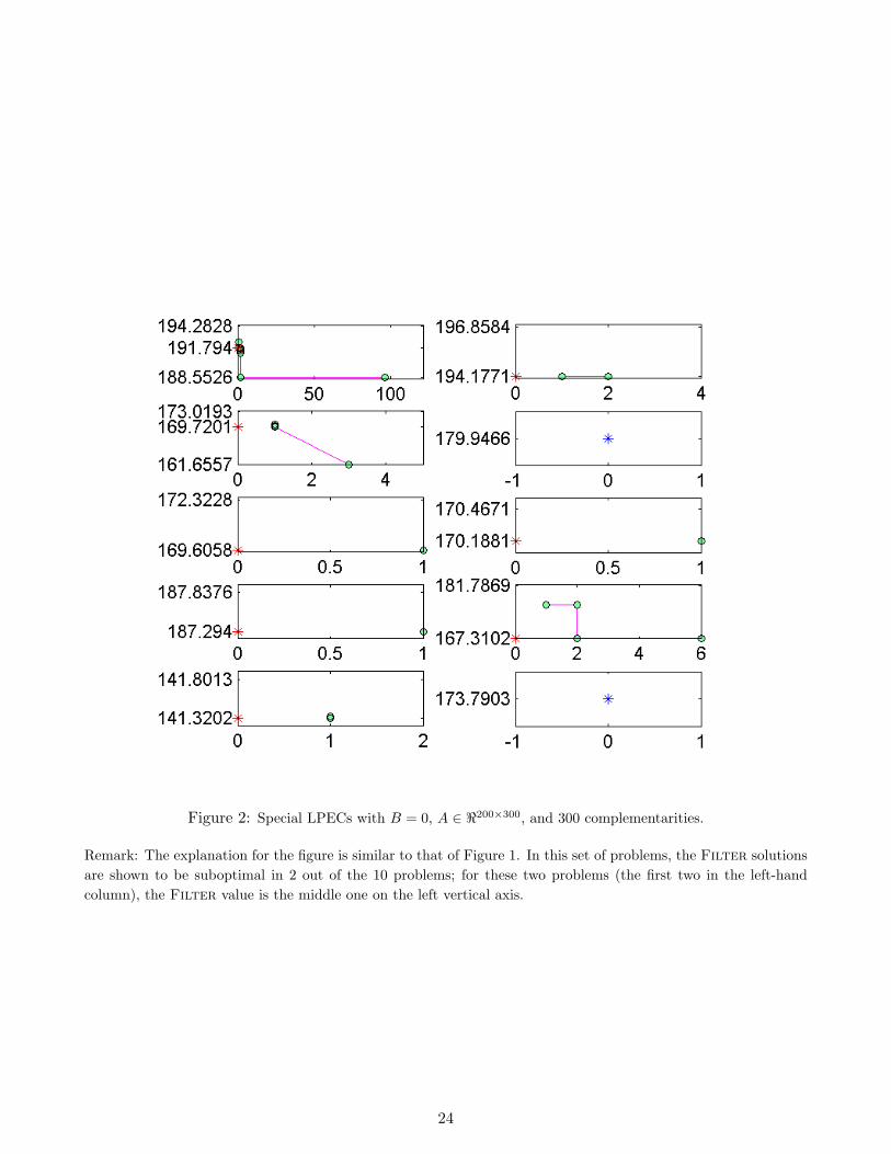
Figure 2: Special LPECs with B = 0, A ∈ <200×300, and 300 complementarities.
Remark: The explanation for the figure is similar to that of Figure 1. In this set of problems, the Filter solutionsare shown to be suboptimal in 2 out of the 10 problems; for these two problems (the first two in the left-handcolumn), the Filter value is the middle one on the left vertical axis.
24

Figure 3: General LPECs with B 6= 0, A ∈ <55×50 and 50 complementarities
Remark: The LPEC feasibility recovery procedure is not employed in the pre-processor; thus there are only 2 valueson the left vertical axis: the Filter value and LPECmin. The Filter solutions are demonstrably suboptimal in allthese runs. There are several problems for which the number of iterations to verify global optimality is considerablymore than others, suggesting that further improvement to the algorithm is possible and that the case B 6= 0 isconsiderably more challenging to solve than the case B = 0.
25