on the herbrandised interpretation for nonstandard arithmetic · on the herbrandised interpretation...
TRANSCRIPT

On the herbrandised interpretation for nonstandardarithmetic
Ana de Almeida Gabriel Vieira Borges
Thesis to obtain the Master of Science Degree in
Mathematics and Applications
Supervisors: Prof. Fernando Ferreira
Prof. Ulrich Kohlenbach
Prof. Carlos Caleiro
Examination Committee
Chairperson: Prof. Cristina SernadasSupervisor: Prof. Fernando Ferreira
Member of the Committee: Prof. Reinhard Kahle
November 2016


Either mathematics is too big for the human mind, or the human mind is more than a machine.Kurt Godel


Acknowledgements
I am grateful to the many, many people who, in one way or another, made this thesis come to life.
In particular, I would like to thank Professor Fernando Ferreira for introducing me to the realm of
proof theory and functional interpretations, for his guidance, for the long hours spent explaining one
thing or another, for his patience, and for the several ideas and suggestions which improved this work.
I am also thankful to Professor Ulrich Kohlenbach for receiving me in Darmstadt, for sharing with
me his enthusiasm for proof mining and the tools necessary for it, for the discussions of interesting
ideas, and for the helpful comments he provided throughout the work.
I would like to thank Professor Carlos Caleiro, for introducing me to the field of functional logic and
for nurturing my interest in the area. I am also very grateful for his availability regarding this thesis.
I thank Bruno Dinis for his help in better understanding nonstandard arithmetic, and Florian Stein-
berg for sharing his knowledge of Weihrauch reducibility.
I am grateful to all the friends who made sure I survived while working on this thesis. In particular,
Raul Penaguiao was an invaluable catalyst from the day I started studying these matters, always
knowing what to say in order to motivate me. He also had helpful suggestions regarding the readability
of this work. Daniel Sousa was a great help during the writing phase, by frequently inquiring about my
progress, by the many conversations which helped maintain my sanity, and finally by helping with the
final revisions and some LATEX troubles. Raquel Goncalves was always available to discuss my work,
and to be the (sometimes much needed) voice of reason. Joao Alırio was the perfect companion while
writing, and always ready to debate anything that crossed my mind regarding what I was working on.
Carolina Caldeirinha has been someone I can always count on for a long, long time, and corrected
numerous grammatical mistakes (I’m sure there are still many more left, fully of my responsibility).
I would also like to thank Pedro Filipe, Marta Cruz, Victor Pecanins, Tome Ribeiro, Maria do Mar
da Camara Pereira, Ana Galhoz, and Diogo Borges for the shared laughs and conversations, and for
working beside me.
Finally, I am grateful to all my family. Each person offered to help and indeed helped by their
constant support. In particular, my mother helped with revising the text, and by listening to my worries.
My father always had an enthusiastic word. Together, they supported me throughout my education,
and particularly made possible my stay in Lisbon during my undergraduate studies, and in Darmstadt
while working on this thesis. My brother was always available for anything I needed. He cooked many
dinners for me, and above all was always happy to listen to the “mathematical stuff” I found most
fascinating at any given time.
v


Abstract
Functional interpretations are useful tools of proof theory. After Godel described his dialectica
interpretation for Heyting arithmetic in 1941, many other interpretations have been proposed, each
focusing on different goals. We start with an overview of the interpretations of Godel and Shoenfield.
We propose a functional interpretation for nonstandard Heyting arithmetic based on previous work
by Van den Berg, Briseid and Safarik. This interpretation enables the transformation of proofs in
nonstandard arithmetic of internal statements into proofs in standard arithmetic of those same state-
ments. The witnesses for external, existential statements of the interpreting formulas are functions
whose output is a finite sequence. Syntactically, the terms representing these functions are called
end-star terms. It is possible to define a preorder of end-star terms. Our interpretation is monotone
over this preorder: if a certain end-star term is a witness for an existential statement, then any “bigger”
term also is. Using this property, we are able to prove a soundness theorem for our interpretation,
which eliminates principles recognisable from nonstandard analysis. From this theorem, we get as
corollary the conservativity of nonstandard arithmetic over standard arithmetic, as well as a term ex-
traction theorem. It is also possible to prove a characterization theorem for our interpretation. As
corollary, we show that the countable saturation principle does not add proof theoretical strength to
our intuitionistic nonstandard system.
Finally, we give a short description of Weihrauch reducibility and comment on an application of
Godel’s dialectica interpretation to, in certain circumstances, prove that a ∀∃-formula Weihrauch re-
duces to another one.
Keywords
Functional interpretations, nonstandard arithmetic, Weihrauch reducibility.
vii


Resumo
As interpretacoes funcionais sao ferramentas uteis da teoria da demonstracao. Depois de Godel
ter descrito a sua interpretacao dialectica para a aritmetica de Heyting, foram propostas muitas outras
interpretacoes, cada uma com objectivos diferentes. Comecamos por apresentar as interpretacoes
de Godel e Shoenfield.
Propomos uma interpretacao funcional para a aritmetica de Heyting nao standard, baseada em
trabalho de Van den Berg, Briseid e Safarik. Esta interpretacao permite a transformacao de provas
na aritmetica nao standard de teoremas internos em provas na aritmetica standard desses mesmos
teoremas. As testemunhas para afirmacoes existenciais externas das formulas interpretadoras sao
funcoes cujo output e uma lista finita. Sintacticamente, os termos que representam estas funcoes
sao chamados termos end-star. E possıvel definir uma pre-ordem nos termos end-star. A nossa
interpretacao e monotona nesta pre-ordem: se um dado termo end-star e uma testemunha para
uma afirmacao existencial, entao qualquer termo “maior” tambem o e. Usando esta propriedade,
provamos a correccao da nossa interpretacao, e eliminamos princıpios reconhecıveis da analise nao
standard. Tambem obtemos como corolario que a aritmetica nao standard e conservativa sobre a ar-
itmetica standard, bem como um teorema de extraccao de termos. E possıvel provar um teorema de
caracterizacao para a nossa interpretacao. Como corolario, mostramos que o princıpio da saturacao
contavel nao acrescenta forca ao nosso sistema intuicionista nao standard.
Por fim, descrevemos brevemente a redutibilidade de Weihrauch e sugerimos uma aplicacao da
interpretacao dialectica de Godel para, em certas circunstancias, decidir se uma formula-∀∃ se reduz-
Weihrauch a outra.
Palavras-chave
Interpretacoes funcionais, aritmetica nao standard, redutibilidade de Weihrauch.
ix


Contents
Acknowledgements . . . . . . . . . . . . . . . . . . . . . . . . . . . . . . . . . . . . . . . . . v
Abstract . . . . . . . . . . . . . . . . . . . . . . . . . . . . . . . . . . . . . . . . . . . . . . . . vii
Resumo . . . . . . . . . . . . . . . . . . . . . . . . . . . . . . . . . . . . . . . . . . . . . . . . ix
1 Introduction 1
1.1 Proof interpretations . . . . . . . . . . . . . . . . . . . . . . . . . . . . . . . . . . . . . . 2
1.2 Interpreting arithmetic . . . . . . . . . . . . . . . . . . . . . . . . . . . . . . . . . . . . . 3
1.3 Interpreting nonstandard arithmetic . . . . . . . . . . . . . . . . . . . . . . . . . . . . . . 4
1.4 Other functional interpretations . . . . . . . . . . . . . . . . . . . . . . . . . . . . . . . . 5
1.5 Weihrauch reducibility . . . . . . . . . . . . . . . . . . . . . . . . . . . . . . . . . . . . . 5
1.6 Thesis outline . . . . . . . . . . . . . . . . . . . . . . . . . . . . . . . . . . . . . . . . . . 6
2 Functional interpretations for arithmetic 7
2.1 Systems for Heyting and Peano arithmetic in all finite types . . . . . . . . . . . . . . . . 8
2.1.1 Extensional and weakly extensional Heyting arithmetic, E-HAω and WE-HAω . . 8
2.1.2 Extensional and weakly extensional Peano arithmetic, E-PAω and WE-PAω . . . 15
2.2 Godel’s dialectica interpretation . . . . . . . . . . . . . . . . . . . . . . . . . . . . . . . . 16
2.3 Shoenfield’s interpretation . . . . . . . . . . . . . . . . . . . . . . . . . . . . . . . . . . . 19
3 Functional interpretations for nonstandard arithmetic 23
3.1 Systems for Heyting and Peano nonstandard arithmetic . . . . . . . . . . . . . . . . . . 24
3.1.1 Heyting and Peano arithmetic with the star type, E-HAω∗ and E-PAω∗ . . . . . . . 24
3.1.2 Heyting and Peano nonstandard arithmetic, E-HAω∗st and E-PAω∗st . . . . . . . . . 30
3.2 Nonstandard principles . . . . . . . . . . . . . . . . . . . . . . . . . . . . . . . . . . . . 32
3.3 The Hst-interpretation . . . . . . . . . . . . . . . . . . . . . . . . . . . . . . . . . . . . . 35
3.4 The Sst-interpretation . . . . . . . . . . . . . . . . . . . . . . . . . . . . . . . . . . . . . . 53
3.5 Countable saturation . . . . . . . . . . . . . . . . . . . . . . . . . . . . . . . . . . . . . . 57
3.5.1 Countable saturation in an intuitionistic setting . . . . . . . . . . . . . . . . . . . 57
3.5.2 Countable saturation in a classical setting . . . . . . . . . . . . . . . . . . . . . . 58
4 A note on Weihrauch reducibility 61
4.1 Weihrauch reducibility . . . . . . . . . . . . . . . . . . . . . . . . . . . . . . . . . . . . . 62
4.2 A comment on how to use the dialectica interpretation to prove reductions . . . . . . . . 63
xi

5 Conclusions and future work 65
5.1 Results . . . . . . . . . . . . . . . . . . . . . . . . . . . . . . . . . . . . . . . . . . . . . 66
5.2 Future work . . . . . . . . . . . . . . . . . . . . . . . . . . . . . . . . . . . . . . . . . . . 66
Bibliography 67
Appendix A Definition of the projection term A-1
xii

1Introduction
Contents1.1 Proof interpretations . . . . . . . . . . . . . . . . . . . . . . . . . . . . . . . . . . . 21.2 Interpreting arithmetic . . . . . . . . . . . . . . . . . . . . . . . . . . . . . . . . . . 31.3 Interpreting nonstandard arithmetic . . . . . . . . . . . . . . . . . . . . . . . . . . 41.4 Other functional interpretations . . . . . . . . . . . . . . . . . . . . . . . . . . . . . 51.5 Weihrauch reducibility . . . . . . . . . . . . . . . . . . . . . . . . . . . . . . . . . . 51.6 Thesis outline . . . . . . . . . . . . . . . . . . . . . . . . . . . . . . . . . . . . . . . 6
1

1.1 Proof interpretations
Given formal systems T1 and T2, a proof interpretation I from T1 to T2 is a particular way of
obtaining a formula AI in the language of T2 from a formula A in the language of T1. Such an
interpretation is defined by induction on the logical structure of A. After defining it, one should be able
to prove a soundness theorem. Soundness theorems are loosely of the form:
Theorem (Soundness). Let C and ∆ be collections of principles, and ∆′ a suitable modification of the
principles ∆. For all formulas A of the language of T1, if T1 + C + ∆ ` A, then T2 + ∆′ ` AI .
The principles C are called characteristic principles. Characteristic principles of a proof interpre-
tation vanish under it. In other words, for a characteristic principle C, it is possible to prove CI in T2without having access to C itself. The principles ∆ are called side principles. Side principles don’t
vanish under I, and we need ∆′ to prove their interpretations. However, the formulas in ∆′ are usually
similar to the formulas in ∆.
Soundness theorems are very useful. For example, as long as ⊥I ≡⊥, which is usually the case,
the soundness theorem for the I-interpretation entails the consistency of T1 + C relative to the consis-
tency of T2.
There is another class of theorems related to proof interpretations: the characterization theorems.
If T is a theory which encompasses the languages of T1 and T2, and P is a collection of principles, a
characterization theorem is of the form:
Theorem (Characterization). For all formulas A of the language of T1, we have that T +P ` A↔ AI .
It is interesting to look for a minimal collection of principles P which is enough to prove the charac-
terization theorem for a given interpretation. These principles give a notion of the “distance” between
the original formula A and its interpretation AI .
The functional interpretations that are discussed in this work are much more specific than what is
outlined above. The theories T1 and T2 are always theories of arithmetic that vary in two important
ways: on the one hand, they feature either Heyting (intuitionistic) or Peano (classical) arithmetic; on
the other hand, they focus on either standard or nonstandard arithmetic. By mixing these four possi-
bilities, four important theories were defined: WE-HAω, which we outline in Section 2.1.1; WE-PAω,
see Section 2.1.2; and E-HAω∗st and E-PAω∗st , discussed in Section 3.1.2.
The “HA” and “PA” stand for Heyting and Peano arithmetic, respectively. The prefixes “WE” and
“E” have to do with the treatment of equality: in the first case the theories are weakly extensional,
while in the second case we allow full extensionality. The “ω” indicates that the theories are typed,
and that we allow all finite types. The “st” means that the theories in question are in a nonstandard
setting. Finally, the “∗” heralds the use of the so-called star types (types for finite sequences), which
will be necessary when we interpret nonstandard arithmetic.
2
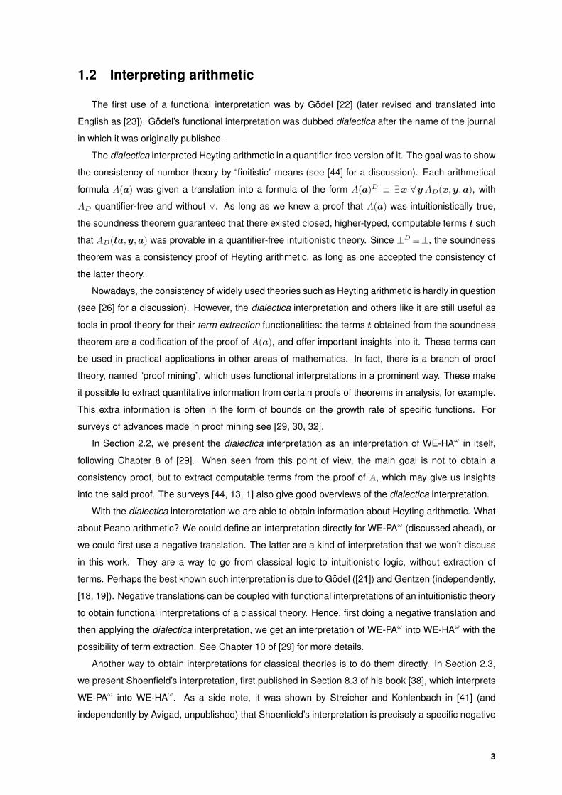
1.2 Interpreting arithmetic
The first use of a functional interpretation was by Godel [22] (later revised and translated into
English as [23]). Godel’s functional interpretation was dubbed dialectica after the name of the journal
in which it was originally published.
The dialectica interpreted Heyting arithmetic in a quantifier-free version of it. The goal was to show
the consistency of number theory by “finitistic” means (see [44] for a discussion). Each arithmetical
formula A(a) was given a translation into a formula of the form A(a)D ≡ ∃x ∀yAD(x,y,a), with
AD quantifier-free and without ∨. As long as we knew a proof that A(a) was intuitionistically true,
the soundness theorem guaranteed that there existed closed, higher-typed, computable terms t such
that AD(ta,y,a) was provable in a quantifier-free intuitionistic theory. Since ⊥D ≡⊥, the soundness
theorem was a consistency proof of Heyting arithmetic, as long as one accepted the consistency of
the latter theory.
Nowadays, the consistency of widely used theories such as Heyting arithmetic is hardly in question
(see [26] for a discussion). However, the dialectica interpretation and others like it are still useful as
tools in proof theory for their term extraction functionalities: the terms t obtained from the soundness
theorem are a codification of the proof of A(a), and offer important insights into it. These terms can
be used in practical applications in other areas of mathematics. In fact, there is a branch of proof
theory, named “proof mining”, which uses functional interpretations in a prominent way. These make
it possible to extract quantitative information from certain proofs of theorems in analysis, for example.
This extra information is often in the form of bounds on the growth rate of specific functions. For
surveys of advances made in proof mining see [29, 30, 32].
In Section 2.2, we present the dialectica interpretation as an interpretation of WE-HAω in itself,
following Chapter 8 of [29]. When seen from this point of view, the main goal is not to obtain a
consistency proof, but to extract computable terms from the proof of A, which may give us insights
into the said proof. The surveys [44, 13, 1] also give good overviews of the dialectica interpretation.
With the dialectica interpretation we are able to obtain information about Heyting arithmetic. What
about Peano arithmetic? We could define an interpretation directly for WE-PAω (discussed ahead), or
we could first use a negative translation. The latter are a kind of interpretation that we won’t discuss
in this work. They are a way to go from classical logic to intuitionistic logic, without extraction of
terms. Perhaps the best known such interpretation is due to Godel ([21]) and Gentzen (independently,
[18, 19]). Negative translations can be coupled with functional interpretations of an intuitionistic theory
to obtain functional interpretations of a classical theory. Hence, first doing a negative translation and
then applying the dialectica interpretation, we get an interpretation of WE-PAω into WE-HAω with the
possibility of term extraction. See Chapter 10 of [29] for more details.
Another way to obtain interpretations for classical theories is to do them directly. In Section 2.3,
we present Shoenfield’s interpretation, first published in Section 8.3 of his book [38], which interprets
WE-PAω into WE-HAω. As a side note, it was shown by Streicher and Kohlenbach in [41] (and
independently by Avigad, unpublished) that Shoenfield’s interpretation is precisely a specific negative
3

translation due to Krivine [34] followed by the dialectica interpretation. So in this case, at least, defining
an interpretation directly for Peano arithmetic is no different from composing a negative translation
with an interpretation for Heyting arithmetic.
1.3 Interpreting nonstandard arithmetic
Interpreting nonstandard arithmetic by way of functional interpretations is a somewhat recent idea
due to Benno van den Berg, Eyvind Briseid and Pavol Safarik [2]. In their paper, they describe
two functional interpretations for intuitionistic and classical logic: the Dst-interpretation, and the Sst-
interpretation, respectively.
In the theories E-HAω∗st and E-PAω∗st there is a unary predicate symbol “st”, which we see as de-
termining whether a given object is standard. This gives rise to two sets of quantifiers: the internal
quantifiers ∀ and ∃, which quantify over all objects, and the external quantifiers ∀st and ∃st, which
quantify only over standard objects. The interpretations of Van den Berg et al. distinguish the treat-
ment of internal and external quantifiers. The external quantifiers are interpreted as usual, requiring
computational witnesses, while the internal quantifiers are exempt from this obligation.
There is another interesting particularity of the Dst-interpretation. It is herbrandised, in the sense
that the witnesses for the external, existential quantifiers of the interpreting formulas need not be
exact; only a finite set of possible witnesses for each statement is required. In this spirit, Van den
Berg et al. impose that the external, existential quantifiers of the interpreting formulas quantify only
over finite sets, which syntactically translates to quantifying over variables of star type. The star type
indicates finite sequences, not sets, but the order of the elements is never relevant.
In accordance with the herbrandised quality of the Dst-interpretation, the interpreting formulas
have a monotonicity property, i.e., if a sequence s is a witness for an external existential statement,
then a “bigger” sequence s′ is also a witness for it. When s and s′ are of star type, we define the
meaning of “bigger” like so: s is contained in s′ if and only if all the elements of s are also elements of
s′.
In Chapter 3 of this work, we present two different interpretations for nonstandard arithmetic: the
Hst and Sst-interpretations, in Sections 3.3 and 3.4, respectively. These interpretations are adapta-
tions of the ones by Van den Berg et al. The key difference between the Hst and Dst-interpretations
is in the external, existential statements of the interpreting formulas: here these variables don’t have
to be of star type, they only have to be of end-star type. Terms of this type represent functions with
several inputs whose last possible output is a finite sequence.
It is possible to extend the preorder of sequences mentioned above to a preorder of the end-star
types. The extension is pointwise, following a suggestion of Fernando Ferreira. For example, if f and
f ′ are of type ρ→ σ → τ∗, we say that f is contained in f ′ if and only if for all x of type ρ and for all y
of type σ, fxy is contained in f ′xy.
The Sst-interpretation described here is due to Dinis and Ferreira [10], even though Van den Berg
et al. also present an interpretation for E-PAω∗st called Sst in Section 7 of [2]. They are very similar (and
4

in fact equivalent in a certain sense), but come from different philosophies: while Van den Berg et al.
obtain their interpretation by coupling the Dst-interpretation with a negative translation and lose the
monotonicity property in the process, Dinis and Ferreira define their Sst-interpretation from scratch
and with monotonicity. Curiously, in the classical setting all external, existential quantifications are
naturally of star type, so the notion of containment between end-star types is never necessary.
1.4 Other functional interpretations
There were a lot of functional interpretations proposed over the years. A comprehensive list can
be found in the historical comments at the end of Chapter 8 of [29]. Here we mention only a couple
of interpretations more.
In [9], Diller and Nahm proposed a modification of the dialectica interpretation which doesn’t need
the decidability of quantifier-free formulas to interpret the A → A ∧ A axiom. The trick is a kind of
herbrandisation. See [8] for a discussion of this interpretation.
In [28], Kohlenbach presented the monotone functional interpretation, which is the dialectica in-
terpretation followed by a weakening of the requirement for the witnessing terms. Instead of requiring
precise witnesses, it requires only majorants for such witnesses. Since it allows for more side princi-
ples, it has been used very successfully as a tool for proof mining. A survey of examples of its use
can be found in [30].
Ferreira and Oliva also have interpretations which only require bounds on the witnessing terms,
called the bounded functional interpretations: [16] for the intuitionistic case, and [14] for the classical
case. Contrary to the monotone functional interpretation, here the bounds are applied at each step of
the interpretations, instead of only at the end. These interpretations were adapted to the nonstandard
setting by Ferreira and Gaspar for the classical case, [15], and by Dinis and Gaspar for the intuitionistic
case, [11].
The bounded functional interpretations share many similarities with the functional interpretations
for nonstandard arithmetic discussed before, since both distinguish between two kinds of quantifiers
(one kind which must produce explicit witnesses and the one kind interpreted uniformly), and both
dispense with precise witnesses, requiring merely some kind of bound.
1.5 Weihrauch reducibility
In Chapter 4, we study a relation between multi-valued operations introduced by Klaus Weihrauch
[45, 46], and later modified to its modern definition by Gherardi and Marcone [20]. It has been used
in logic to find which theorems can be computationally (or continuously) reduced into which other
(see, for example, [5, 6, 7, 20]). To deal with this, we look at theorems as multi-valued operations. In
particular, theorems of the form:
∀x ∃ y A0(x, y)
are good candidates to see as multi-valued operations, since to every x it’s possible to assign at least
a y such that A0(x, y).
5

With this notion it is possible to define the so-called Weihrauch degrees, which are classes of
inter-reducible theorems, thus obtaining a classification of theorems. In this work we don’t classify
any theorem, but instead give a suggestion on how to, in certain circumstances, prove that a ∀∃-
theorem Weihrauch-reduces to another, by way of the dialectica interpretation.
1.6 Thesis outline
We start by introducing the two best known functional interpretations in Chapter 2: Godel’s (Sec-
tion 2.2) and Shoenfield’s (Section 2.3). These are interpretations for Heyting and Peano arithmetic
in all finite types, respectively. So the first step is to introduce formal systems for these two theories.
That is done in Section 2.1.1 for Heyting arithmetic, and in Section 2.1.2 for Peano arithmetic. Then
we give the statements of the soundness, term extraction, and characterization theorems for both
interpretations.
In Chapter 3, we move into the realm of nonstandard arithmetic. We start by adapting the systems
introduced in Section 2.1: first by adding the star type, meant to describe finite sequences, in Section
3.1.1; then by adding the unary “st” predicate, meant to describe the standardness of a term, in
Section 3.1.2.
In Section 3.2, we describe proof principles often used in the context of nonstandard arithmetic.
These principles will be eliminated by the functional interpretations we present in the ensuing sections.
In Section 3.3, we introduce the Hst-interpretation. This is a functional interpretation for nonstan-
dard Heyting arithmetic, based on the Dst-interpretation of Van den Berg et al. [2]. The key difference
is in the allowed types of the witnesses for the external, existential statements of the interpreting
formulas. We prove soundness, term extraction, and characterization theorems for this new interpre-
tation.
In Section 3.4, we describe the Sst-interpretation of Dinis and Ferreira [10], a functional interpre-
tation for nonstandard Peano arithmetic. We extend the soundness theorem of this interpretation to
a theory of full arithmetic, since in [10] the theory considered only allows induction for quantifier-free
formulas. We also prove a characterization theorem for this interpretation.
In Section 3.5, we put the Hst-interpretation to use. We start by showing, in Section 3.5.1, that
the principle of countable saturation, CSATω, does not add power to an intuitionistic theory. Then,
in Section 3.5.2, we note that that, when CSATω is added to the classical theory of nonstandard
arithmetic we use, the ensemble interprets full second-order arithmetic.
In Section 4.1, we introduce the notion of Weihrauch reducibility between multi-valued operations.
Finally, Section 4.2 is a short note describing how to use Godel’s interpretation of Section 2.2 to, in
certain circumstances, prove that a ∀∃-theorem Weihrauch-reduces to another one.
6

2Functional interpretations for
arithmetic
Contents2.1 Systems for Heyting and Peano arithmetic in all finite types . . . . . . . . . . . . 8
2.1.1 Extensional and weakly extensional Heyting arithmetic, E-HAω and WE-HAω . 82.1.2 Extensional and weakly extensional Peano arithmetic, E-PAω and WE-PAω . . 15
2.2 Godel’s dialectica interpretation . . . . . . . . . . . . . . . . . . . . . . . . . . . . . 162.3 Shoenfield’s interpretation . . . . . . . . . . . . . . . . . . . . . . . . . . . . . . . . 19
7

2.1 Systems for Heyting and Peano arithmetic in all finite types
We use several formalizations of arithmetic throughout this work, both in the intuitionistic and the
classical settings. This section describes what we mean by Heyting and Peano arithmetic in all finite
types. Along the way, we mention various useful results, mostly without proof. For an overview of
these topics, see Chapter 3 of [29].
In order to present the typed systems of this section, we need to first define what we mean by
type.
Definition 2.1.1 (Finite types). The finite types are described inductively as:
• 0 is a finite type;
• If ρ, τ are finite types, then (ρ→ τ) is a finite type.
The parenthesis in a type associate to the right, and we omit them when possible, to simplify the
notation.
The type 0 should be thought of as the natural numbers, and the type ρ→ τ as the functions from
objects of type ρ to objects of type τ . As a side note, the type 0→ 0, also represented by the symbol 1,
is the type of the functions from the natural numbers to the natural numbers. It is also the appropriate
type for the real numbers, which can be represented by Cauchy sequences of rational numbers. See
[29] for a description on how to formalize analysis.
Remark 2.1.2. Any type ρ 6= 0 can be uniquely written as ρ = ρ1 → ρ2 → · · · → ρk → 0, for some
natural number k and types ρ1, . . . , ρk.
2.1.1 Extensional and weakly extensional Heyting arithmetic, E-HAω and WE-HAω
Extensional and weakly extensional Heyting arithmetic in all finite types, represented by E-HAω
and WE-HAω respectively, share the same terms, formulas and most axioms. The distinction is made
in the axioms of equality for types higher than 0, as we will see shortly.
Terms
• A numerable set of variables for each type: xσ, yσ, zσ, . . .;
• Logical constants or combinators:
– Πρ,τ of type ρ→ τ → ρ, for all types ρ, τ ;
– Σδ,ρ,τ of type (δ → ρ→ τ)→ (δ → ρ)→ δ → τ , for all types δ, ρ, τ ;
• Arithmetical constants:
– 0 of type 0 (zero);
– S of type 0→ 0 (successor);
8

– (Rρ) = (R1)ρ, . . . , (Rk)ρ where ρ = ρ1, . . . , ρk and each Ri has type:
0→ ρ1 → · · · → ρk → (0→ ρ1 → · · · → ρk → ρ1)→ · · · → (0→ ρ1 → · · · → ρk → ρk)→ ρi
for all natural numbers k, and types ρ1, . . . , ρk (simultaneous recursors);
• If tτ , fτ→σ are terms, then (ft)σ is a term.
The type of a term is often omitted to avoid heavy notation. But every time a term is mentioned,
it should be assumed that it has a type consistent with the context in which it appears, obeying the
application of terms rule.
We think of (fτ→σtτ ) as “f applied to t”, as if f were a unary function and t an argument. However,
if σ = ρ → δ, the same term f could appear in the expression ((fτ→ρ→δtτ )uρ), and now it looks like
it should be a binary function. In reality, all of the options above are valid term constructions, as long
as the types are correct. The parenthesis associate to the left, which means that ftu is the same as
((ft)u).
The expression t is a (possibly empty) tuple of terms t1, . . . , tk, where |t| := k. In particular, we
use t, s := t1, . . . , tk, s1, . . . , sl, ft := ft1 · · · tk and ft := f1t, . . . , fnt.
The variables of a term t, denoted by var(t), are defined inductively in the following way: if x is a
variable, var(x) := {x}; if c is a constant (logical or arithmetical), var(c) := ∅; if tτ , fτ→σ are terms,
var(ft) := var(f) ∪ var(t). If a term t has no variables, i.e., if var(t) = ∅, we say that t is closed.
Formulas
• ⊥ is an atomic formula (falsum);
• If t0, u0 are terms, then t =0 u is an atomic formula (equality of type 0);
• If A and B are formulas and xτ is a variable, then (A ∧ B), (A ∨ B), (A → B), (∀xτ A) and
(∃xτ A) are formulas.
We use (¬A) as shorthand for (A →⊥), (t 6=0 u) as shorthand for ¬(t =0 u) and (A ↔ B) as
shorthand for ((A→ B) ∧ (B → A)).
In order to facilitate the reading of formulas, it is possible to omit some sets of parenthesis. This is
governed by the following priority of symbols, from higher (left) to lower (right):
• ¬, ∀, ∃ • ∧, ∨ • →,↔
Furthermore, → associates to the right, i.e., A → B → C is to be interpreted as A → (B → C),
which makes for even lighter notation.
Formulas without both ∀ and ∃ are said to be quantifier-free, and are sometimes marked as so
with an underscore “0”, i.e., A0, B0, . . . represent quantifier-free formulas.
If A0 is a quantifier-free formula, B ≡ ∀xA0 and C ≡ ∃xA0 for some tuple of variables x, we say
that B is a purely universal formula, and that C is a purely existential formula.
9

The free variables of a formula A, denoted by fv(A), are defined inductively in the following way:
fv(⊥) := ∅; if t0, u0 are terms, fv(t =0 u) := var(t) ∪ var(u); if A,B are formulas, fv(A�B) :=
fv(A) ∪ fv(B), with � ∈ {∧,∨,→}; if A is a formula and x is a variable, fv(4xA) := fv(A) \ {x}, with
4 ∈ {∀,∃}. Variables which are not free but do appear in the formula are said to be bound.
If a formula has no free variables, we say that it is a closed formula, or a sentence. When we write
A(x), we mean that x might be a free variable of A (but never a bound variable of A), and we wish to
bring it to attention.
Logical axioms and rules
Heyting arithmetic is based on intuitionistic logic. The axioms that we use for it are:
Contraction: A→ A ∧A A ∨A→ A
Weakening: A ∧B → A A→ A ∨B
Symmetry: A ∧B → B ∧A A ∨B → B ∨A
Ex falso quodlibet : ⊥→ A
Quantifier: ∀xA→ A[t/x] A[t/x]→ ∃xA where t is free for x in A
The notation A[t/x] represents formula A where variable x is replaced by t in every place where x
appears free, i.e., in every place where it is not in the scope of a quantification over x. The substitution
can only be made when it doesn’t lead to previously free variables in t becoming bound in A[t/x]. If
the substitution is possible, we say that t is free for x in A. It is conventional to assume that, in a
context where we wish to replace x for t in formula A, but t is not free for x in A, we just rename the
bound variables in A until the substitution causes no problems, obtaining A′. This is possible because
the name of a bound variable is for all intents and purposes irrelevant, meaning that A and A′ are
equivalent. After implementing this convention, there is no longer a need to mention whether a term
is free for a variable in a formula or not.
When we use the axiom ∀xA → A[t/x], we say that we are instantiating x by t, and often write
x := t.
The logical rules are:
A A→ B
B
Modus ponens:A→ B B → C
A→ C
Syllogism:
A ∧B → C
A→ B → C
Exportation:A→ B → C
A ∧B → C
Importation:
A→ B
C ∨A→ C ∨B
Expansion:
10

B → A
B → ∀xA, x 6∈ fv(B)
∀-introduction:A→ B
∃xA→ B, x 6∈ fv(B)
∃-introduction:
There are many other descriptions of intuitionistic logic, using other axioms and rules. This one,
first alluded to by Godel in [22], is particularly useful for proving theorems about it, which is our pur-
pose. Still, it would be possible to use a natural deduction description to obtain the same goals, as is
done in [25]. Natural deduction makes proving assertions inside the language much more straightfor-
ward. For an overview of a natural deduction calculus for intuitionistic logic, including descriptions of
semantics for it, see, for example, Chapters 2 and 9 of [42].
Equality
Following Chapter 3 of [29], we take type 0 equality as primitive with the following axioms:
Reflexivity: x =0 x
Symmetry: x =0 y → y =0 x
Transitivity: x =0 y ∧ y =0 z → x =0 z
Equality at higher types is defined: let ρ = ρ1 → · · · → ρk → 0 be a type, and t, u terms of type ρ.
Then:
(t =ρ u) :≡ (∀ yρ11 , . . . , yρkk ty1 . . . yk =0 uy1 . . . yk)
where y1, . . . , yk are not variables of either t or u.
Sometimes we omit the subscript of the equality symbol to lighten the notation. It can be inferred
from the types of the terms being compared. Conversely, if we write t =ρ u, then it is implicit that both
t and u have type ρ.
Reflexivity, symmetry and transitivity of =ρ follow from the same axioms for type zero equality. But
there’s still something missing. Even though our system does not have functions of arity greater than
zero, it does have typed constants, which take their place. So it would seem reasonable to ask for
some kind of extensionality axioms, for example:
Eρ,τ : ∀ fρ→τ , xρ, yρ (x =ρ y → fx =τ fy)
for all pairs of types (ρ, τ).
When accepting the axioms of extensionality, we obtain extensional Heyting arithmetic, E-HAω. In
this context it is possible to prove:
Proposition 2.1.3 (Equal terms are interchangeable in E-HAω). For every formula A, and variables
xρ, yρ, E-HAω proves:
x =ρ y ∧A(x)→ A(y)
Proof. Induction on the logical structure of A. For the base case it is necessary to prove x =ρ y →
t[x/z] =τ t[y/z] by induction on the structure of the terms.
11

However, the soundness theorem for the dialectica interpretation (Theorem 2.2.6) does not hold
in the context of E-HAω, precisely because of the extensionality axioms (see [24]). In order to weaken
them, we use a quantifier-free extensionality rule:
QF-ER :A0 → t =ρ u
A0 → r[t/x] =τ r[u/x]
where A0 is a quantifier-free formula, xρ is a variable and tρ, uρ and rτ are terms.
When accepting QF-ER in lieu of the Eρ,τ axioms, we obtain weakly extensional Heyting arith-
metic, WE-HAω. In this context we can only prove a weaker version of Proposition 2.1.3, namely:
Proposition 2.1.4. For any quantifier-free formula A0 and formula B, WE-HAω proves:
A0 → t =ρ u
A0 → (B[t/xρ]↔ B[u/xρ])
There is another way to weaken E-HAω to a theory suitable to perform the soundness of the
dialectica interpretation, namely to take equality as intensional. This is actually what Godel does
when describing his interpretation in [22]. For a discussion of the several possible treatments of
equality, see Section 2.5 of [1].
Arithmetical axioms and rules
Successor axioms:
Sx 6=0 0 Sx =0 Sy → x =0 y
Π and Σ axioms:
Πρ,τxy =ρ x, for any xρ, yτ
Σδ,ρ,τxyz =τ xz(yz), for any xδ→ρ→τ , yδ→ρ, zδ
Recursor axioms: let ρ = ρ1, . . . , ρk be any tuple of types. Let x0, y = y1, . . . , yk with each yi of
type ρi, and z = z1, . . . , zk with each zi of type 0→ ρ1 → · · · → ρk → ρi be variables. The axioms
are:(Ri)ρ0yz =ρi yi
(Ri)ρ(Sx)yz =ρi zix(Rρxyz)for i ∈ {1, . . . , k}
We changed the order of the arguments of the zi’s, compared to what is done in [29]. This is to
simplify the construction of some terms ahead.
Induction schema:
A(0) ∧ ∀x0 (A(x)→ A(Sx))→ ∀xA(x)
We could have equivalently introduced the induction rule instead of the induction schema:
A(0) A(x)→ A(Sx)
A(x)
12

Useful definitions and results
Our first goal is to show that quantifier-free formulas satisfy the law of excluded middle when in
the presence of arithmetic. To achieve it, some preliminary results are necessary.
Lemma 2.1.5. WE-HAω ` ∀x0 (x =0 0 ∨ x 6=0 0).
Idea of Proof. Induction on x0.
Lemma 2.1.6. WE-HAω proves the following:
1. x =0 y ↔ |x− y| =0 0
2. x =0 0 ∧ y =0 0↔ x+ y =0 0
3. x =0 0 ∨ y =0 0↔ x · y =0 0
4. (x =0 0→ y =0 0)↔ sign(x) · y =0 0
where |x − y|, x + y and x · y have the usual meaning and sign(x) is 0 when x 6=0 0 and S0 when
x =0 0.
Idea of Proof. It should be clear that the functions used here are primitive recursive and hence that it
is possible to define suitable terms for them in WE-HAω, making use of recursion.
The proof of the equivalences goes by double induction on x, y and uses Lemma 2.1.5.
Proposition 2.1.7. Let A0(x) be a quantifier-free formula of WE-HAω, with free variables among x.
Then there exists a closed term tA0such that:
WE-HAω ` ∀x (tA0x =0 0↔ A0(x))
Idea of Proof. Induction on the logical structure of A0.
Notice that the atomic formulas of WE-HAω are either ⊥ or of the form t =0 u for terms t and u.
Clearly WE-HAω ` 0 =0 S0↔⊥, so even ⊥ can be seen as an equality between terms.
The result then follows from Lemma 2.1.6: item 1 takes care of the base of induction for atomic
formulas other than ⊥, and the other three items of the steps for each logical symbol: ∧, ∨, and →,
respectively.
Corollary 2.1.8 (Law of excluded middle for quantifier-free formulas). If A0 is a quantifier-free formula
of the language of WE-HAω, then:
WE-HAω ` A0 ∨ ¬A0
Proof. Direct from Lemma 2.1.5 and Proposition 2.1.7.
Corollary 2.1.9 (Elimination of ∨). For every quantifier-free formulaA0(x) of the language of WE-HAω,
there exists an equivalent quantifier-free formula B0(x) without ∨.
Proof. Simply take B0(x) :≡ (tA0x =0 0), as given by Proposition 2.1.7. This is an atomic formula,
and clearly doesn’t have any ∨.
13

The next results focus on providing us with a very convenient way of expressing terms, namely
λ-abstraction.
Definition 2.1.10 (λ-abstraction).
• (λxρ . x)ρ→ρ := Σρ,σ→ρ,ρΠρ,σ→ρΠρ,σ
• (λxρ . tσ)ρ→σ := Πσ,ρt, if x 6∈ var(t)
• (λxρ . tσ→τuσ)ρ→τ := Σρ,σ,σ→τ (λx . t)(λx . u), if x ∈ var(tu)
Remark 2.1.11. var(λx . t) = var(t) \ {x}, as can be clearly seen by induction on the construction of
the lambda terms.
One easily shows by induction on the construction of the lambda terms that:
Proposition 2.1.12 (Combinatorial completeness). WE-HAω ` (λxρ . tτ )sρ =τ t[s/x].
We often write λx, y . t as shorthand for λx . (λ y . t). Furthermore, the notation λx . t should be
interpreted as (λx1, . . . , xk . t1), . . . , (λx1, . . . , xk . tl).
Corollary 2.1.13. For every term tτ and variable xρ, there exists a term T of type ρ→ τ and variables
var(T ) = var(t) \ {x} such that:
WE-HAω ` Tsρ =τ t[s/x]
Proof. Taking T := λx . t, this is a direct consequence of Remark 2.1.11 and Proposition 2.1.12.
We close with the descriptions of some useful terms, namely a zero of arbitrary type, and definition
by cases.
Definition 2.1.14 (Oρ). For each type ρ = ρ1 → · · · → ρk → 0, we distinguish a “zero of type ρ”:
Oρ = λxρ11 , . . . , xρkk . 0
This zero will be useful when we need a term of a specific type, but the term in itself is not relevant.
Proposition 2.1.15 (Definition by cases). For every type ρ, there exists a closed term C such that:
WE-HAω ` ∀x0, yρ, zρ [(x = 0→ Cxyz = y) ∧ (x 6= 0→ Cxyz = z)]
Proof. Let
C := λx0, yρ, zρ . Rρxy(λ r0, qρ . z)
Notice that C is well defined, for Rρ has type 0 → ρ → (0 → ρ → ρ) → ρ, x has type 0, y has type ρ
and λ r0, qρ . z has type 0→ ρ→ ρ. Furthermore:
C0yz =ρ Rρ0y(λ r0, qρ . z)
=ρ y
C(Sx)yz =ρ Rρ(Sx)y(λ r0, qρ . z)
=ρ (λ r0, qρ . z)x(Rρxy(λ r0, qρ . z))
=ρ z
14

It only remains to notice that, as x 6=0 0 → x = S(predx) (where pred0→0 is the predecessor term),
then x 6=0 0→ Cxyz =ρ z.
Proposition 2.1.15 can be proven even without the use of Rρ: the base type recursor R0 suffices.
This is shown in Proposition 3.19 of [29].
Remark 2.1.16. It should be clear that all of the results outlined above for WE-HAω also hold for
E-HAω, since they share the same language and one can derive the quantifier-free rule of extension-
ality from the extensionality axioms.
2.1.2 Extensional and weakly extensional Peano arithmetic, E-PAω and WE-PAω
Peano arithmetic is obtained from Heyting arithmetic by using classical logic instead of intuitionistic
logic. One way to do this is to maintain everything and add a new logical axiom, the law of excluded
middle for all formulas:
LEM : A ∨ ¬A
Hence WE-PAω is WE-HAω + LEM, and E-PAω is E-HAω + LEM.
However, these definitions now have superfluous axioms and rules. Furthermore, one can obtain
some logical connectives from others. This is a nuisance when one wants to prove something about
a system of Peano arithmetic by induction on the logical structure of a formula, or by induction on the
proof of a statement.
A minimal treatment of classical logic is, for example, to take ∨, ¬, and ∀ as primitive, and ⊥,∧,
→, and ∃ as defined. Following Section 2.6 of [38], the logical axioms and rules can be reduced to:
A ∨ ¬A
LEM:
∀xA→ A[t/x]
Instantiation:
A
A ∨B
Expansion:A ∨AA
Contraction:
A ∨ (B ∨ C)
(A ∨B) ∨ C
Association:A ∨B ¬A ∨ C
B ∨ C
Cut:
A ∨B∀xA ∨B
, x 6∈ fv(B)
∀-introduction:
Remark 2.1.17. All the results from Section 2.1.1 proved in E-HAω or WE-HAω also hold for their
classical counterparts.
15

The most obvious model of these systems is the set-theoretical: the objects of type 0 are the
natural numbers, and the objects of type ρ → τ are all the set-theoretical functionals from objects of
type ρ to objects of type τ . There are other models; for example, it is possible to only allow sequen-
tially continuous functionals, or only majorizable functionals. For a discussion of several models, see
Section 3.6 of [29].
2.2 Godel’s dialectica interpretation
In this section, we give an overview of Godel’s dialectica interpretation for intuitionistic arithmetical
formulas. It was first published as [22] in the dialectica journal, hence the name of the interpretation.
Here we follow Chapter 8 of [29].
Definition 2.2.1 (D-interpretation). The D-interpretation (also known as Godel’s or dialectica inter-
pretation) associates to each formula A in the language of WE-HAω a formula AD of the form
AD ≡ ∃x ∀yAD(x,y)
with the same free variables and in the same language as A. The (possibly empty) variable tuples x
and y and their types are uniquely determined by the logical structure of A. It is important that these
variables do not appear free in A. The formula AD(x,y) is quantifier-free and without ∨. The definition
proper is given below. The sub-formulas inside square brackets are the formulas corresponding to
the AD above.
• If A is an atomic formula, AD :≡ AD :≡ A
Given the interpretations AD ≡ ∃x ∀yAD(x,y) and BD ≡ ∃u ∀vBD(u,v):
• (A ∧B)D :≡ ∃x,u ∀y,v [AD(x,y) ∧BD(u,v)]
• (A ∨B)D :≡ ∃ z0,x,u ∀y,v [(z = 0→ AD(x,y)) ∧ (z 6= 0→ BD(u,v))]
• (A→ B)D :≡ ∃U ,Y ∀x,v [AD(x,Y xv)→ BD(Ux,v)]
• (∃ z A(z))D :≡ ∃ z,x ∀y [AD(x,y, z)]
• (∀ z A(z))D :≡ ∃X ∀ z,y [AD(Xz,y, z)]
Remark 2.2.2 (Trivial D-interpretations).
1. (AD)D ≡ AD, and consequently (A�B)D ≡ (AD �BD)D, for � ∈ {∧,∨,→} and (4xA)D ≡
(4xAD)D, for 4 ∈ {∀,∃}.
2. If A0 is a quantifier-free formula without ∨, then AD0 ≡ A.
3. If A ≡ 4xA0 with A0 a quantifier-free formula without ∨ and 4 ∈ {∀,∃}, then AD ≡ A.
16

From now on we assume that all quantifier-free formulas are without ∨, possible by Corollary 2.1.9,
which permits the use of Remark 2.2.2 without problems.
The dialectica interpretation is almost, but not quite, a way of formalizing the ideas of the Brouwer-
Heyting-Kolmogorov interpretation, described, for example, in Section 2.1 of [42]. Actual formaliza-
tions are Kleene’s realizability, introduced in [27], and Kreisel’s modified realizability, introduced in
[33].
What distinguishes the D-interpretation is the treatment of implication. A motivation for its defini-
tion can be found in Section 8.1 of [29]. In the case of the realizability interpretations, realizers of an
implication don’t worry about occurrences of ∀ in the premise. Since negation is in fact an implication,
this means that the weak existential quantifier ¬∀¬ is not given a proper witness.
Godel’s interpretation is much more demanding. All occurrences of some kind of existential quan-
tification, be it in the form of disjunction, universal quantification in a premise or actual strong existen-
tial quantification must be catalogued and witnessed. A more thorough discussion of these topics can
be found in [31].
We make use of three principles, which are characteristic principles of the dialectica interpretation
(for reasons which will be made clear ahead), and we need their definitions:
Definition 2.2.3 (ACω). The schema of choice, ACω, is the union for all finite types ρ and τ of:
ACρ,τ : ∀xρ ∃ yτ A(x, y)→ ∃Y ρ→τ ∀xρA(x, Y x)
where A is any formula of the language of WE-HAω.
Definition 2.2.4 (Mω). Markov’s principle, Mω, is the union for all tuples of finite types ρ of:
Mρ : ¬∀xρA0(x)→ ∃xρ ¬A0(x)
where A0 is a quantifier-free formula of the language of WE-HAω.
Definition 2.2.5 (IPω∀ ). The independence of premise schema for purely universal premises, IPω∀ , is
the union for all finite types ρ of:
IPρ∀ : (∀xA0(x)→ ∃ yρB(y))→ ∃ yρ (∀xA0(x)→ B(y))
where A0 is a quantifier-free formula of the language of WE-HAω, and y is not free in A0.
Theorem 2.2.6 (Soundness of the D-interpretation). Let A(a) be an arbitrary formula of the language
of WE-HAω, containing only a free, such that A(a)D ≡ ∃x ∀yAD(x,y,a). Furthermore, let ∆∀ be a
collection of purely universal sentences in the same language. Suppose:
WE-HAω + ACω + IPω∀ + Mω + ∆∀ ` A(a)
Then there are closed terms t, which can be extracted from a proof of A(a), such that:
WE-HAω + ∆∀ ` ∀yAD(ta,y,a)
17

Idea of Proof. Induction on the proof of A. For each axiom possibly used in such a proof, we must
provide witnessing closed terms t for the existentially quantified variables of its D-interpretation. Sim-
ilarly, we must provide witnessing terms for the conclusions of each rule possibly used in the proof of
A, assuming by induction hypothesis that we already have access to such terms for the premises of
the rule.
This means that the full proof is very long, as there are a considerable number of axioms and
rules to take into account. It is however not terribly complicated. Most terms needed are simple
projections and the proof of ∀yAD(ta,y,a) usually ends with the very same axiom or rule which is
under consideration.
A notable exception is the axiom A→ A ∧A. The first step to obtain (A→ A ∧A)D is to find AD.
Each of the three instances of AD should have different names for the bound variables, so that there
is no confusion. So let’s say that the free variables of A are in a, that AD ≡ ∃x ∀yAD(x,y,a), and
use the pairs (u,v) and (z,w) for the other two instances. Then:
(A→ A ∧A)D ≡ ∃U ,Z,Y ∀x,v,w (AD(x,Y xvw,a)→ AD(Ux,v,a) ∧AD(Zx,w,a)) (2.2.1)
Take tU := tZ := λa,x .x, and:
tY := λa,x,v,w .
{v if ¬AD(x,v,a)
w if AD(x,v,a)
Notice that we can define tY as shown, because, as AD(x,v,a) is a quantifier-free formula, by
Proposition 2.1.7 we know that there exists a closed term t such that:
WE-HAω ` txva = 0↔ AD(x,v,a)
which means that checking whether AD(x,v,a) holds is the same as checking whether txva = 0.
The terms tY can then be defined with the help of Proposition 2.1.15.
We now need to show that replacing in (2.2.1) the existentially quantified U , Z and Y by their
respective terms followed by a produces a provable formula, namely:{∀x,v, r (AD(x,v,a)→ AD(x,v,a) ∧AD(x, r,a)) if ¬AD(x,v,a)
∀x,v, r (AD(x, r,a)→ AD(x,v,a) ∧AD(x, r,a)) if AD(x,v,a)
But it is clear that in both cases the formulas are provable in WE-HAω, so we are done.
The full proof can be found in Section 8.2 of [29].
The aforementioned principles (ACω, Mω and IPω∀ ) are said to be characteristic principles of the
dialectica interpretation because they are not needed to prove their own D-interpretations. In fact, the
interpretations of these three principles are instances of A→ A.
Theorem 2.2.7 (Program extraction by theD-interpretation). Let ∀x ∃yA0(x,y) be a sentence in the
language of WE-HAω, with A0 quantifier-free. Furthermore, let ∆∀ be a collection of purely universal
formulas. Suppose:
WE-HAω + ACω + Mω + IPω∀ + ∆∀ ` ∀x ∃yA0(x,y)
18

Then there are closed terms t such that:
WE-HAω + ∆∀ ` ∀xA0(x, tx)
Proof. Direct consequence of Theorem 2.2.6, taking into account that:
(∀x ∃yA0(x,y))D ≡ ∃Y ∀xA0(x,Y x)
When in the presence of these characteristic principles, we can prove the equivalence between a
formula and its dialectica interpretation:
Theorem 2.2.8 (Characterization theorem for theD-interpretation). For all formulas A in the language
of WE-HAω:
WE-HAω + ACω + Mω + IPω∀ ` A↔ AD
Proof. Induction on the logical structure ofA. In each case, the implicationAD → A is straightforward.
For A → AD, the only cases which are not intuitionistic truths are those of universal quantification
and implication. For the first, the axiom of choice is needed. For the second, we make use of all three
principles.
2.3 Shoenfield’s interpretation
Shoenfield’s interpretation, or S-interpretation, was proposed by Shoenfield in Section 8.3 of his
book [38]. It is an interpretation of WE-PAω in WE-HAω, as opposed to Godel’s, which only interprets
WE-HAω in itself.
Definition 2.3.1 (The S-interpretation). The S-interpretation (also known as Shoenfield’s interpreta-
tion) associates to each formula A in the language of WE-PAω a formula AS of the form
AS ≡ ∀x ∃yAS(x,y)
with the same free variables and in the same language as A. The (possibly empty) variable tuples
x and y and their types are uniquely determined by the logical structure of A. It is important that
these variables do not appear free in A. The formula AS(x,y) is quantifier-free. The definition proper
is given below. The sub-formulas inside square brackets are the formulas corresponding to the AS
above.
• If A is an atomic formula, AS :≡ AS :≡ A
Given the interpretations AS ≡ ∀x ∃yAS(x,y) and BS ≡ ∀u ∃vBS(u,v):
• (¬A)S :≡ ∀Y ∃x [¬AS(x,Y x)]
• (A ∨B)S :≡ ∀x,u ∃y,v [AS(x,y) ∨BS(u,v)]
• (∀ z A(z))S :≡ ∀ z,x ∃y [AS(x,y, z)]
19

Lemma 2.3.2 (S-interpretation of some formulas).
Let A0 be a quantifier-free formula. Then:
• AS0 ≡ A0
• (∀ zA0)S ≡ ∀zA0
Taking AS ≡ ∀x ∃yAS(x,y) and BS ≡ ∀u ∃vBS(u,v), WE-PAω proves:
• (A→ B)S ↔ ∀Y ,u ∃x,v [AS(x,Y x)→ BS(u,v)]
• (A ∧B)S ↔ ∀X,U ∃Y ,V [AS(XY V ,Y (XY V )) ∧BS(UY V ,V (UY V ))]
• (∃ z A(z))S ↔ ∀X ∃ z,Y [AS(XzY ,Y (XzY ), z)]
The S-interpretation of ∧ looks unnecessarily complicated. After all it seems like
(A ∧B)S ≡ ∀x,u ∃y,v [AS(x,y) ∧BS(u,v)]
would have been possible and certainly more straightforward. This is in fact true, as shown in Section
4 of [41].
Definition 2.3.3 (QF-ACω). The quantifier-free schema of choice, QF-ACω, is the restriction of ACω
to quantifier-free formulas. So it is the union for all finite types ρ, τ of:
QF-ACρ,τ : ∀xρ ∃yτ A0(x,y)→ ∃Y ρ→τ ∀xρA0(x,Y x)
where ρ→ τ is an abuse of notation which should be read as
ρ1 → · · · → ρk → τ1, . . . , ρ1 → · · · → ρk → τl
for ρ = ρ1, . . . , ρk and τ = τ1, . . . , τl, and A0 is a quantifier-free formula of the language of WE-PAω.
We need to define QF-ACω for tuples of variables, because, contrary to what happens with ACω,
it would not possible to apply QF-ACω to a formula several times in a row to make up for the lack of
tuples in the definition (not all the subformulas would be quantifier-free).
Theorem 2.3.4 (Soundness of the S-interpretation). Let A(a) be an arbitrary formula of the language
of WE-PAω, containing only a free, such that A(a)S ≡ ∀x ∃yAS(x,y,a). Furthermore, let ∆∀ be a
collection of purely universal sentences in the same language. Suppose:
WE-PAω + QF-ACω + ∆∀ ` A(a)
Then there are closed terms t, which can be extracted from a proof of A(a), such that:
WE-HAω + ∆∀ ` ∀xAS(x, tax,a)
Shoenfield gives a proof of a similar result to this in Section 8.3 of his book [38]. Gaspar presents
a full direct proof in Section 5.1 of [17], but he uses intensional instead of weakly-extensional equality.
The treatment of the quantifier-free extensionality rule (QF-ER) is therefore missing. But it uses the
20

same idea as in the soundness of the dialectica interpretation. Finally, by observing that Shoenfield’s
interpretation can be factored in Krivine’s negative translation and Godel’s dialectica, as shown in
[41], the soundness of the S-interpretation is also a consequence of the soundness of these two
interpretations. More details can be found in Chapter 10 of [29].
Corollary 2.3.5 (Relative consistency). WE-PAω is consistent relative to WE-HAω.
Proof. Consequence of Theorem 2.3.4 when applied to ⊥, since ⊥S ≡⊥.
Theorem 2.3.6 (Program extraction by the S-interpretation). Let ∀x ∃ y A0(x, y) be a sentence in the
language of WE-PAω, with A0 quantifier-free. Furthermore, let ∆∀ be a collection of purely universal
formulas. Suppose:
WE-PAω + QF-ACω + ∆∀ ` ∀x ∃ y A0(x, y)
Then there is a closed term t such that:
WE-HAω + ∆∀ ` ∀xA0(x, tx)
Proof. Consequence of Theorem 2.3.4, taking into account that:
(∀x ∃ y A0(x, y))S ≡ ∀x ∃ y ¬¬A0(x, y)
and that quantifier-free formulas are decidable in WE-HAω (Corollary 2.1.8).
Theorem 2.3.7 (Characterization theorem for the S-interpretation). For all formulas A of the language
of WE-PAω:
WE-PAω + QF-ACω ` A↔ AS
Proof. By induction on the logical structure of A. The only step that needs QF-ACω is the step for the
negation. The full proof can be found in Section 5.1 of [17].
21

22

3Functional interpretations for
nonstandard arithmetic
Contents3.1 Systems for Heyting and Peano nonstandard arithmetic . . . . . . . . . . . . . . 24
3.1.1 Heyting and Peano arithmetic with the star type, E-HAω∗ and E-PAω∗ . . . . . 243.1.2 Heyting and Peano nonstandard arithmetic, E-HAω∗
st and E-PAω∗st . . . . . . . . 30
3.2 Nonstandard principles . . . . . . . . . . . . . . . . . . . . . . . . . . . . . . . . . . 323.3 The Hst-interpretation . . . . . . . . . . . . . . . . . . . . . . . . . . . . . . . . . . . 353.4 The Sst-interpretation . . . . . . . . . . . . . . . . . . . . . . . . . . . . . . . . . . . 533.5 Countable saturation . . . . . . . . . . . . . . . . . . . . . . . . . . . . . . . . . . . 57
3.5.1 Countable saturation in an intuitionistic setting . . . . . . . . . . . . . . . . . . 573.5.2 Countable saturation in a classical setting . . . . . . . . . . . . . . . . . . . . 58
23

It can be seen by compactness arguments that there are nonstandard models of arithmetic, i.e.,
models not isomorphic to the natural numbers (Section 12.3 of [4]; see also Chapter 25 of the same
book). It turns out that working in a nonstandard setting is a great way of formalizing reasoning about
infinitesimals and infinitely big numbers.
Nonstandard analysis was popularized by Abraham Robinson [37]. After him, several people
presented nonstandardness in different ways. Particularly relevant for us is the work of Nelson, who
developed an axiomatization of nonstandard analysis named Internal Set Theory (IST) [35]. IST is
Zermelo-Fraenkel set theory with choice (ZFC), plus a new predicate “st” for “being standard”, and
three new axioms: idealization, standardization and transfer. Nelson proved that IST is conservative
over ZFC: any internal formula (not containing “st”) provable in IST is already provable in ZFC.
It was noted by Benno van den Berg, Eyvind Briseid and Pavol Safarik [2] that the algorithm pre-
sented by Nelson in [36] to show the conservativity of IST over ZFC is remarkably similar to Shoen-
field’s functional interpretation [38]. From this observation, Van den Berg et al. developed a functional
interpretation for nonstandard Heyting arithmetic, named the Dst-interpretation [2]. They worked in
E-HAω∗st , a formal system with higher types.
Our goal for Section 3.1 is to present the system E-HAω∗st , as well as its classical variant, E-PAω∗st ,
introduced in [2]. These systems are E-HAω and E-PAω, extended with a new type construction, the
star type, and with a new predicate, the “st” predicate, in the spirit of Nelson’s IST.
In Section 3.2, we describe some principles common in nonstandard settings, which will appear in
the ensuing sections in prominent ways.
Section 3.3 is dedicated to the Hst-interpretation, a functional interpretation for nonstandard Hey-
ting arithmetic (E-HAω∗st ) similar to the Dst-interpretation of Van den Berg et al. In Section 3.4 we
present the Sst-interpretation of Dinis and Ferreira [10], which can be thought of as the Hst-interpreta-
tion’s classical counterpart.
Finally, Section 3.5 is dedicated to the principle of countable saturation. We present the work of
Van den Berg et al. [3], who showed that this principle is weak intuitionistically, but when added to a
classical setting, the ensemble interprets full second-order arithmetic.
3.1 Systems for Heyting and Peano nonstandard arithmetic
3.1.1 Heyting and Peano arithmetic with the star type, E-HAω∗ and E-PAω∗
We want to extend the terms of E-HAω and E-PAω to include finite sequences. Actually, what we
really want is to represent finite sets, but finite sequences are simpler and enough for our purposes.
There is a new type to represent these finite sequences: the star type. We extend Definition 2.1.1
(Finite types) to include it:
• If ρ is a finite type, then ρ∗ is a finite type.
The type ρ∗ should be thought of as representing the finite sequences of elements of type ρ. Note
that we have been talking about tuples of terms, and they should not be confused with sequences. A
24

tuple t is shorthand for the terms tρ11 , . . . , tρkk , each with possibly different types. A sequence xρ
∗is a
specific term which semantically represents an ordered finite list of terms of type ρ: xρ0, . . . , xρn−1.
E-HAω∗ and E-PAω∗ share the same terms. The only difference between them is that E-HAω∗ is
based on intuitionistic logic, while E-PAω∗ is based on classical logic.
Terms
In addiction to the terms of E-HAω and E-PAω described in Section 2.1.1, E-HAω∗ and E-PAω∗ also
have terms to deal with the sequences:
• {}ρ of type ρ∗, for all types ρ (empty sequence);
• prepρ of type ρ→ ρ∗ → ρ∗, for all types ρ (prepend an element to a sequence);
• (L)σ,ρ = (L1)σ,ρ, . . . , (Lk)σ,ρ where ρ = ρ1, . . . , ρk and each Li has type:
σ∗ → ρ1 → · · · → ρk → (σ → ρ1 → · · · → ρk → ρ1)→ · · · → (σ → ρ1 → · · · → ρk → ρk)→ ρi
for all types σ,ρ (simultaneous list recursors);
• Πρ,τ , Σδ,ρ,τ and (R)σ where the types ρ, τ, δ and σ vary over all the types, including the new
ones.
We slightly changed the notation from what is presented in [2], in order to be more consistent with
the notation of [10], which we adopt.
Formulas
The same formulas as E-HAω (respectively E-PAω), with terms in the language of E-HAω∗ (respec-
tively E-PAω∗).
Equality
Following [2], we take equality as primitive in all types. The axioms are the following:
Reflexivity: x =ρ x
Symmetry: x =ρ y → y =ρ x
Transitivity: x =ρ y ∧ y =ρ z → x =ρ z
Left congruence: x =ρ y → fx =τ fy
Right congruence: f =ρ→τ g ↔ ∀x (fx =τ gx)
25

Axioms and rules
• Logical axioms and rules of E-HAω (respectively E-PAω) accounting for the new formulas avail-
able (since there are new terms);
• Axioms for Π,Σ and R accounting for the new types available;
• List recursor axioms: let ρ = ρ1, . . . , ρk be any tuple of types. Let xσ, sσ∗, y = y1, . . . , yk with
each yi of type ρi, and z := z1, . . . , zk with each zi of type σ → ρ1 → · · · → ρk → ρi be variables.
The axioms are:
(Li)σ,ρ{}σyz =ρi yi
(Li)σ,ρ(prepσ xs)yz =ρi zix(Lσ,ρsyz)for i ∈ {1, . . . , k}
We changed the order of the arguments of the zi’s, compared to what is done in [2]. This is to
simplify the construction of some terms ahead.
• Sequence axiom: ∀ sρ∗ (s = {}ρ ∨ ∃xρ, wρ∗s = prepρ xw).
Useful Definitions and Results
Proposition 3.1.1 (Equal terms are interchangeable in E-HAω∗). For every formula A of its language,
E-HAω∗ proves:
x = y ∧A(x)→ A(y)
Proof. As in Proposition 2.1.3, this is done by induction on the logical structure of A. Even though
now equality is a primitive notion, the same proof holds.
Proposition 3.1.2. E-HAω∗ is a definitional extension of E-HAω. Likewise, E-PAω∗ is a definitional
extension of E-PAω.
Proof. This follows from the fact that we can already talk about sequences in E-HAω (respectively in
E-PAω) by making use of the terms available to code them, like is done in pages 58–60 of [29].
Our goal now is to define some useful notions to deal with terms of star type, such as what we
mean by the length of a sequence, an element of a sequence, and so on. We also define a preorder
over these terms.
Definition 3.1.3 (| · |ρ, (·)·,ρ). We define length and projection terms:
• Length: | · |ρ of type ρ∗ → 0, defined as:
| · |ρ := λ sρ∗. Lρ,0s0(λxρ, n0 . Sn)
We write |t| instead of | · |t. Using the axioms of L, we obtain:
|{}| = 0
|prepxs| = S|s|
26

• Projection: (·)·,ρ of type ρ∗ → 0 → ρ, defined in appendix A. We write (s)i instead of (·)·si. We
need the following properties:
({})i = O
(prepxs)0 = x
(prepxs)(Si) = (s)i
Definition 3.1.4 (∈). If xρ, sρ∗
are terms:
x ∈ρ s :≡ ∃ i0 <0 |s| x = (s)i
where <0 is definable already in WE-HAω such that it has the expected properties (see Section 3.5 of
[29] for more details).
Lemma 3.1.5 (Induction schema for sequences).
E-HAω∗ ` ϕ({}ρ) ∧ ∀xρ, sρ∗
(ϕ(s)→ ϕ(prepxs))→ ∀ sρ∗ϕ(s)
Proof. One first shows using the sequence axiom that:
1. ∀ sρ∗ (|s| = 0↔ s = {})
2. ∀n0, sρ∗ (|s| = Sn↔ ∃xρ, wρ∗ (s = prepρ xw ∧ |w| = n))
This effectively reduces sequence induction to ordinary induction, by considering the statement:
∀n0, sρ∗
(|s| = n→ ϕ(s))
Definition 3.1.6 ({·}ρ,∪ρ,⋃ρ,τ ). We define terms that construct a singleton sequence, the union of
two sequences and the indexed union of several sequences.
• Singleton: {·}ρ of type ρ→ ρ∗, defined as:
{·}ρ := λxρ . prepρ x{}ρ
We write {x} instead of {·}x.
• Union: ∪ρ of type ρ∗ → ρ∗ → ρ∗, defined as:
∪ρ := λ tρ∗, uρ
∗. Lρ,ρ∗tuprepρ
We write t ∪ u instead of ∪tu. Using the axioms of L, we obtain:
{} ∪ u = u
(prepxt′) ∪ u = prepx(t′ ∪ u)
27

• Indexed union:⋃ρ,τ of type (ρ→ τ∗)→ ρ∗ → τ∗, defined as:
⋃ρ,τ := λ fρ→τ
∗, tρ∗. Lρ,τ∗t{}(λ a, s . ((fa) ∪ s))
We write⋃x∈t fx instead of
⋃ft. Using the axioms of L, we obtain:
⋃x∈{} fx = {}⋃x∈(prep at′) fx = (fa) ∪
⋃x∈t′ fa
Following the spirit of [10], we use the following three properties of the just defined terms to prove
the soundness theorems of the functional interpretations ahead (Theorems 3.3.9 and 3.4.5). Notice,
however, that since we have access to full arithmetic, we define the terms differently, making use of
the list recursors.
Lemma 3.1.7. E-HAω∗ proves:
1. x ∈ {x}
2. x ∈ t ∨ x ∈ u→ x ∈ t ∪ u
3. y ∈ t ∧ z ∈ fy → z ∈⋃x∈t fx
Proof.
1. We need to show:
∃ i < |{x}| x = ({x})i
Since |{x}| = 1 and ({x})0 = x, taking i := 0 suffices.
2. We need to show:
(∃ i < |t| x = (t)i) ∨ (∃ j < |u| x = (u)j)→ (∃ k < |t ∪ u| x = (t ∪ u)k)
First notice that |t ∪ u| = |t| + |u|, which can be shown using induction over the sequence t.
Then check that ∀ i < |t| (t)i = (t ∪ u)i, and that ∀ j < |u| (u)j = (t ∪ u)|t|+j , both by sequence
induction over t. With this in mind, the result is trivial.
3. We need to show:
(∃ i < |t| y = (t)i) ∧ (∃ j < |fy| z = (fy)j)→ (∃ k < |⋃x∈t fx| z = (
⋃x∈t fx)k)
First notice that |⋃x∈t fx| =
∑i<|t| |f(t)i|, which can be seen by sequence induction on t. Given
i, j as in the assumption, take k :=∑l<i |f(t)l|+ j. This works, which can be seen by sequence
induction on t.
It is possible to define a preorder on the star typed terms:
28

Definition 3.1.8 (⊆τ ). Given terms t, u of type τ∗:
t ⊆τ u :≡ ∀ i < |t| ∃ j < |u| (t)i = (u)j
Remark 3.1.9. The relation ⊆ is both reflexive and transitive.
Notice that the order of the elements in the sequences t and u is not relevant to determine whether
t ⊆ u. This is in accordance with the fact that we are thinking of terms of star type as stand ins for
sets.
We can obtain as corollary from Lemma 3.1.7 a similar result for sequences:
Lemma 3.1.10. E-HAω∗ proves:
1. x ∈ t ∧ t ⊆ t′ → x ∈ t′
2. x ⊆ t ∨ x ⊆ u→ x ⊆ t ∪ u
3. y ∈ t ∧ z ⊆ fy → z ⊆⋃x∈t fx
This concludes everything we need for terms of star type. However, there is another class of terms
in which we are interested: the terms of end-star type.
Remark 3.1.11. Remark 2.1.2 no longer holds with the star types. Now it is also possible for a term
to have type ρ = ρ1 → · · · → ρk → τ∗.
Definition 3.1.12 (End-star types). If ρ = ρ1 → · · · → ρk → τ∗, for some natural number k ≥ 0 and
types ρ1, . . . , ρk, τ , we say that ρ is an end-star type.
We are going to need a preorder between terms of end-star type. The following is an idea due to
Fernando Ferreira, which works for our interpretation in a very elegant way.
Definition 3.1.13 (vρ,τ ). Given a tuple of types ρ = ρ1, . . . , ρk and terms f, g of end-star type
ρ1 → · · · → ρk → τ∗:
f vρ,τ g :≡ ∀xρ fx ⊆τ gx
In the case where ρ is the empty tuple, vρ,τ reduces to ⊆τ .
Remark 3.1.14. The relation v is both reflexive and transitive.
Since we are going to work a lot with terms of end-star type, we define constants akin to ∪ and⋃
(Definition 3.1.6) in order to concatenate terms of this special kind of type.
Definition 3.1.15 (tρ,τ ,⊔σ,ρ,τ ). We define terms akin to ∪ and
⋃, only for inputs of end-star type
instead of star type.
• tρ,τ of type (ρ1 → · · · → ρk → τ∗) → (ρ1 → · · · → ρk → τ∗) → (ρ1 → · · · → ρk → τ∗), defined
as:
tρ,τ := λ tρ1→···→ρk→τ∗, uρ1→···→ρk→τ
∗. (λxρ . (tx) ∪ (ux))
We write t t u instead of ttu.
29

•⊔σ,ρ,τ of type (σ → ρ1 → · · · → ρk → τ∗)→ σ∗ → (ρ1 → · · · → ρk → τ∗), defined as:⊔
σ,ρ,τ := λ fσ→ρ1→···→ρk→τ∗, tσ∗. (λyρ .
⋃x∈t fxy)
We write⊔x∈t fx instead of
⊔ft.
Using Lemma 3.1.10, it is easy to check that the following properties of t and⊔
hold. We will use
them in the proof of the soundness theorem of the Hst-interpretation, Theorem 3.3.9.
Lemma 3.1.16. E-HAω∗ proves:
1. x v t ∨ x v u→ x v t t u
2. y ∈ t ∧ z v fy → z v⊔x∈t fx
Definition 3.1.17 (Monotonicity). If x is of end-star type, we say that the formula A(x) is monotone
(or upward closed) in x if:
∀ y (x v y ∧A(x)→ A(y))
Definition 3.1.18 (Oρ). Taking into account Remark 3.1.11, we need to define (closed) terms Oρ
where ρ is an end-star type:
Oρ1→···→ρk→τ∗
:= λxρ11 , . . . , xρkk . {Oτ}
Remark 3.1.19. All the results proved in E-HAω∗ during this section also hold in E-PAω∗.
3.1.2 Heyting and Peano nonstandard arithmetic, E-HAω∗st and E-PAω∗
st
Now it is time to introduce systems to deal with nonstandardness: E-HAω∗st and E-PAω∗st . These will
be extensions of E-HAω∗ and E-PAω∗, respectively. The terms remain the same, but we add some
new formulas.
Formulas
• All formulas of the language of E-HAω∗ are formulas of E-HAω∗st and all the formulas of the
language of E-PAω∗ are formulas of E-PAω∗st ;
• If tρ is a term, stρ t is an atomic formula;
• For E-HAω∗st : if xρ is a variable and A is a formula, ∀st xρA and ∃st xρA are formulas.
• For E-PAω∗st : ∀st xA(x) is defined as shorthand for ∀x (¬ stx∨A(x)), and ∃st xA(x) as shorthand
for ¬∀x (¬ stx ∨ ¬A(x)).
Definition 3.1.20 (Internal and external formulas). An internal formula is a formula in the language
of E-HAω∗ (or E-PAω∗), i.e., without any st, ∀st x or ∃st x. An external formula is a formula which is not
internal.
We adopt an important convention, the same as Nelson in [36] and Van den Berg et al. in [2, 3]:
from now on internal formulas are represented by lower-case Greek letters. Upper-case Latin letters
represent formulas which can be external.
We say that formulas of the form ∀st xϕ(x), with ϕ an internal formula, are ∀st-formulas.
30
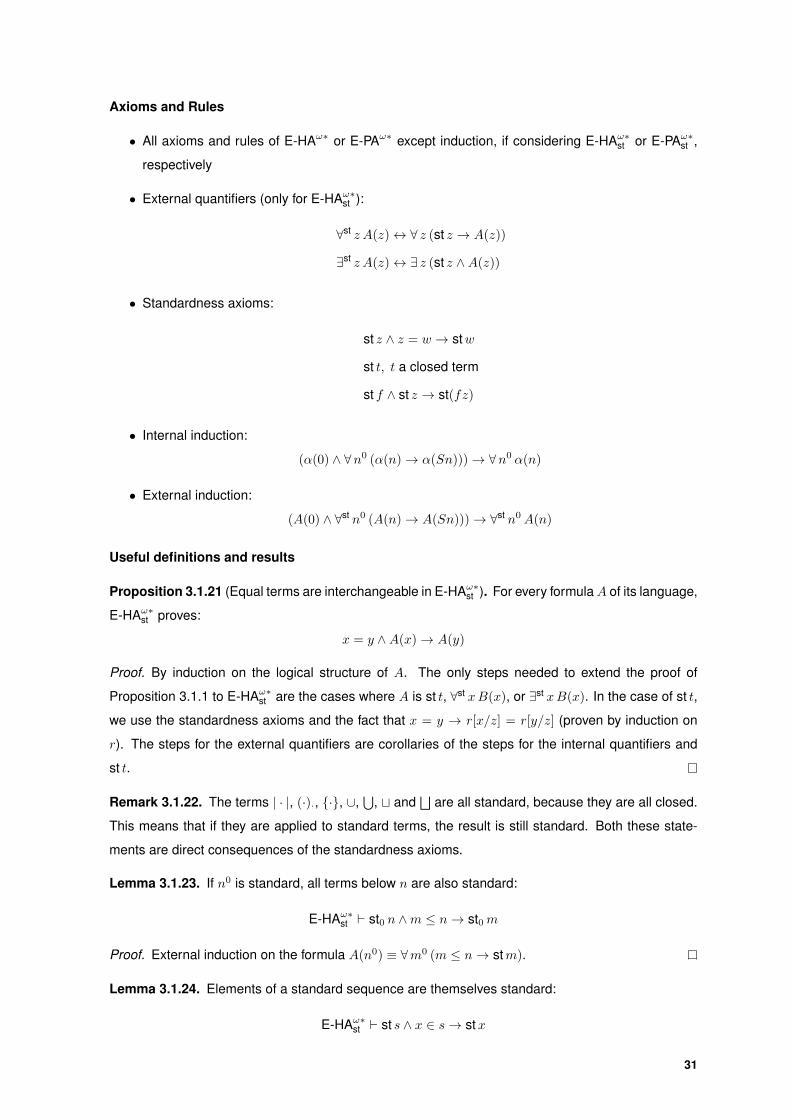
Axioms and Rules
• All axioms and rules of E-HAω∗ or E-PAω∗ except induction, if considering E-HAω∗st or E-PAω∗st ,
respectively
• External quantifiers (only for E-HAω∗st ):
∀st z A(z)↔ ∀ z (st z → A(z))
∃st z A(z)↔ ∃ z (st z ∧A(z))
• Standardness axioms:
st z ∧ z = w → stw
st t, t a closed term
st f ∧ st z → st(fz)
• Internal induction:
(α(0) ∧ ∀n0 (α(n)→ α(Sn)))→ ∀n0 α(n)
• External induction:
(A(0) ∧ ∀st n0 (A(n)→ A(Sn)))→ ∀st n0A(n)
Useful definitions and results
Proposition 3.1.21 (Equal terms are interchangeable in E-HAω∗st ). For every formulaA of its language,
E-HAω∗st proves:
x = y ∧A(x)→ A(y)
Proof. By induction on the logical structure of A. The only steps needed to extend the proof of
Proposition 3.1.1 to E-HAω∗st are the cases where A is st t, ∀st xB(x), or ∃st xB(x). In the case of st t,
we use the standardness axioms and the fact that x = y → r[x/z] = r[y/z] (proven by induction on
r). The steps for the external quantifiers are corollaries of the steps for the internal quantifiers and
st t.
Remark 3.1.22. The terms | · |, (·)·, {·}, ∪,⋃
, t and⊔
are all standard, because they are all closed.
This means that if they are applied to standard terms, the result is still standard. Both these state-
ments are direct consequences of the standardness axioms.
Lemma 3.1.23. If n0 is standard, all terms below n are also standard:
E-HAω∗st ` st0 n ∧m ≤ n→ st0m
Proof. External induction on the formula A(n0) ≡ ∀m0 (m ≤ n→ stm).
Lemma 3.1.24. Elements of a standard sequence are themselves standard:
E-HAω∗st ` st s ∧ x ∈ s→ stx
31

Proof. We recall that x ∈ s ≡ ∃ i < |s| x = (s)i. Assuming st s, it is clear by Remark 3.1.22 that |s|
is standard. Then by Lemma 3.1.23 we get st i. This is enough to show st (s)i, which means, by the
first standardness axiom, that stx.
Remark 3.1.25. All the results proved in E-HAω∗st during this section also hold in E-PAω∗st .
Definition 3.1.26 (Internalization). For every formula A of the language of E-HAω∗st , we define its
internalization, Aint, in the language of E-HAω∗, as the formula obtained from A by replacing every
occurrence of st z by z = z, and every occurrence of ∀st z and ∃st z by ∀ z and ∃ z, respectively.
Similarly, the internalization of a formula in the language of E-PAω∗st is obtained by replacing all
instances of st z by z = z.
Proposition 3.1.27. E-HAω∗st is a conservative extension of E-HAω∗. Likewise, E-PAω∗st is a conserva-
tive extension of E-PAω∗.
Proof. It suffices to show that the internalization of the external axioms of E-HAω∗st (respectively
E-PAω∗st ) are provable in E-HAω∗ (respectively in E-PAω∗), which is straightforward.
3.2 Nonstandard principles
We have defined a system, E-HAω∗st , which, despite being intended for nonstandard arithmetic,
still admits the standard model (Proposition 3.1.27). In other words, the existence of nonstandard
elements is never imposed. This changes when we start to consider nonstandard principles.
Definition 3.2.1 (OSω). The overspill principle, OSω, is the union for all finite types ρ of:
OSρ : ∀st xρ ϕ(x)→ ∃xρ (¬ stx ∧ ϕ(x))
where ϕ is any internal formula in the language of E-HAω∗st .
Proposition 3.2.2. The overspill principle implies the existence of nonstandard objects of any type.
Proof. Just take ϕ(x) ≡ (x = x) in OSω, obtaining:
∃xρ (¬ stx)
Definition 3.2.3 (Iω). The idealization principle, Iω, is the union for all finite types ρ and τ of:
Iρ,τ : ∀st z′ρ∗∃wτ ∀ z ∈ z′ ϕ(z, w)→ ∃wτ ∀st zρ ϕ(z, w)
where if ρ = ρ1, . . . , ρk, then ρ∗ = ρ∗1, . . . , ρ∗k, the expression ∀ z ∈ z′ is ∀ z1 ∈ z′1 · · · ∀ zk ∈ z′k, and ϕ
is an internal formula in the language of E-HAω∗.
We wish to show that idealization implies overspill. For that, we need an auxiliary lemma:
Lemma 3.2.4. There is no standard sequence of type ρ∗ which holds every standard term of type ρ:
E-HAω∗st ` ∀st z′ρ∗∃st wρ ∀ z ∈ z′ (z 6= w)
32

Proof. By induction on the type ρ.
ρ = 0
Let z′0∗
be an arbitrary standard sequence. Since z′ is standard, it has a standard finite number
of elements. Simply take w as the successor of the maximum element of z′. Then clearly w is
standard and w 6∈ z′.
ρ = σ → τ
Let z′(σ→τ)∗
be an arbitrary standard sequence. By induction hypothesis:
∀st u′τ∗∃st vτ ∀u ∈ u′ (u 6= v) (3.2.1)
Take in (3.2.1) u′ :=⋃z∈z′{zOσ}, and let v be a standard term such that ∀u ∈ u′ (u 6= v). We
now prove that w := λxσ . v is such that ∀ z ∈ z′ (z 6= w). Let z ∈ z′ be arbitrary and suppose
z =σ→τ w. Then in particular zOσ =τ wOσ. By definition of w, this means that zOσ =τ v. But
this is a contradiction, since zOσ ∈ u′ and v was chosen precisely so that v 6∈ u′.
ρ = σ∗
Let z′σ∗∗
be an arbitrary standard sequence. By induction hypothesis:
∀st u′σ∗∃st vσ ∀u ∈ u′ (u 6= v) (3.2.2)
Take in (3.2.2) u′ :=⋃z∈z′ z and let v be a standard term such that ∀u ∈ u′ (u 6= v). We now
prove that w := {v} is such that ∀ z ∈ z′ (z 6= w). Let z ∈ z′ be arbitrary and suppose z =σ∗ w.
By definition of w, this means z =σ∗ {v}. But this is a contradiction, since on the one hand
z ⊆ u′ by definition of u′, and on the other hand v 6∈ u′ by hypothesis on v, which means that
{v} 6⊆ u′.
Proposition 3.2.5. E-HAω∗st + Iω ` OSω.
Proof. We prove that we get OSω for a general internal formula ψ from Iω for the formula ϕ(z, w) ≡
z 6= w ∧ ψ(w). That is, given:
∀st z′ρ∗∃wρ ∀ z ∈ z′ (z 6= w ∧ ψ(w))→ ∃wρ ∀st zρ (z 6= w ∧ ψ(w)) (3.2.3)
we show:
∀st xρ ψ(x)→ ∃xρ (¬ stx ∧ ψ(x)) (3.2.4)
Notice that the consequent of (3.2.3) implies the consequent of (3.2.4), so the only thing it remains to
guarantee is:
∀st xρ ψ(x)→ ∀st z′ρ∗∃wρ ∀ z ∈ z′ (z 6= w ∧ ψ(w)) (3.2.5)
Assume the antecedent of (3.2.5) and let z′ be standard but otherwise arbitrary. Take w standard
such that ∀ z ∈ z′ (z 6= w), as given by Lemma 3.2.4. Then it only remains to show ψ(w). But since
w is standard, this is a consequence of the assumption ∀st xψ(x).
33

The realization principle, so named in [2], is the contrapositive of the idealization principle. Hence
in a classical context it is a consequence of Iω.
Definition 3.2.6 (Rω). The realization principle, Rω, is the union for all finite types ρ and τ of:
Rρ,τ : ∀wρ ∃st zτ ϕ(z, w)→ ∃st z′τ∗∀wρ ∃ z ∈ z′ ϕ(z, w)
where ϕ is any internal formula in the language of E-PAω∗.
Lemma 3.2.7 (Rω for monotone formulas). If z is of end-star type and ϕ(z, w) is monotone on z (for
any w), then Rω reduces to:
∀wρ ∃st zτ ϕ(z, w)→ ∃st zτ ∀wρ ϕ(z, w)
Proof. It is enough to show:
∃st z′τ∗∀wρ ∃ z ∈ z′ ϕ(z, w)→ ∃st zτ ∀wρ ϕ(z, w)
After fixing z′ in the antecedent, take in the consequent z :=⊔v∈z′ v. This is a standard term (remem-
bering that z′ is standard itself) and does the job.
When we are in an intuitionistic context, the realization principle Rω will not be enough. We need
a version for external formulas:
Definition 3.2.8 (NCRω). The non-classical realization principle, NCRω, is the union for all finite types
ρ, τ of:
NCRρ,τ : ∀wρ ∃st zτ A(z, w)→ ∃st z′τ∗∀wρ ∃ z ∈ z′ A(z, w)
where A is any formula in the language of E-HAω∗st .
Lemma 3.2.9 (NCRω for monotone formulas). If z if of end-star type and A(z, w) is monotone on z
(for any w), then NCRω reduces to:
∀wρ ∃st zτ A(z, w)→ ∃st zτ ∀wρA(z, w)
Proof. Same as Lemma 3.2.7.
The non-classical realization principle owes its name to the fact that, when added to E-HAω∗st , it
entails the undecidability of the standardness predicate, as is shown by Proposition 3.5 of [2].
Definition 3.2.10 (LLPOωst). The lesser limited principle of omniscience, LLPOω
st, is the union for all
types ρ and τ of:
LLPOρ,τst : ∀st z′ρ
∗, w′τ
∗(∀ z ∈ z′ ϕ(z) ∨ ∀w ∈ w′ ψ(w))→ ∀st zρ ϕ(z) ∨ ∀st wτ ψ(w)
where ϕ,ψ are any internal formulas of the language of E-HAω∗.
The proof of the next lemma uses an idea of [11] (where LLPOωst in their context is the bounded
universal disjunction principle, BUDω).
34

Lemma 3.2.11. E-HAω∗st + Iω ` LLPOωst.
Proof. Assume:
∀st z′ρ∗, w′τ
∗(∀ z ∈ z′ ϕ(z) ∨ ∀w ∈ w′ ψ(w)) (3.2.6)
It is easy to check that (3.2.6) implies:
∀st z′, w′ ∃n0 ((n =0 0→ ∀ z ∈ z′ ϕ(z)) ∧ (n 6=0 0→ ∀w ∈ w′ ψ(w)))
which, after some manipulation, gives us:
∀st z′, w′ ∃n ∀ z ∈ z′ ∀w ∈ w′ ((n =0 0→ ϕ(z)) ∧ (n 6=0 0→ ψ(w))) (3.2.7)
Applying Iρ,τ,0 to (3.2.7), we obtain:
∃n ∀st z, w ((n =0 0→ ϕ(z)) ∧ (n 6=0 0→ ψ(w)))
Since, as seen in Lemma 2.1.5, equality of type 0 is decidable in WE-HAω, and by extension in
E-HAω∗st , we know that either n =0 0 or n 6=0 0. In the first case we are able to prove ∀st z ϕ(z), and in
the second we prove ∀st wψ(w). Hence we obtain the desired formula:
∀st z ϕ(z) ∨ ∀st wψ(w)
These are all the nonstandard principles we will need. For more details about them, and for other
nonstandard principles in the context of E-HAω∗st , see Section 3 of [2].
3.3 The Hst-interpretation
We now introduce an adaptation of Godel’s dialectica interpretation for nonstandard arithmetic:
the herbrandised functional interpretation, or Hst-interpretation. It is heavily based in Van den Berg,
Briseid, and Safarik’s Dst-interpretation introduced in Section 5 of [2]. The main difference is in the
treatment of the existentially quantified variables: while Van den Berg et al. require these variables to
be of star type, here we just require them to be of end-star type.
There is another small difference: here we change the clause for the disjunction. We do this in
order to be able to do the verification of the soundness theorem intuitionistically. In [2], the step for
the expansion rule of the proof of the soundness theorem for the Dst-interpretation, though classically
true, does not seem to hold in E-HAω∗. This was pointed out by Fernando Ferreira, after wondering
about the dissimilarity between the disjunction clauses of the Dst-interpretation, and the bounded
functional interpretation [16], when the other clauses are so strikingly similar.
Definition 3.3.1 (Hst-interpretation). The Hst-interpretation associates to each formula A of E-HAω∗st
a formula AHst of the form:
AHst ≡ ∃st x ∀st y αHst(x,y)
35

with the same free variables and in the same language as A. The (possibly empty) variable tuples x
and y and their types are uniquely determined by the logical structure of A. It is important that these
variables do not appear free in A. Furthermore, αHst is an internal formula.
The definition proper is given below. The sub-formulas inside square brackets are the internal
formulas corresponding to the αHst above.
• αHst :≡ αHst :≡ α for internal atomic formulas α
• (st z)Hst :≡ ∃st z′ [z ∈ z′]
Given the interpretations AHst ≡ ∃st x ∀st y αHst(x,y) and BHst ≡ ∃st u ∀st v βHst(u,v):
• (A ∧B)Hst :≡ ∃st x,u ∀st y,v [αHst(x,y) ∧ βHst(u,v)]
• (A ∨B)Hst :≡ ∃st x,u ∀st y′,v′ [∀y ∈ y′ αHst(x,y) ∨ ∀v ∈ v′ βHst(u,v)]
• (A→ B)Hst :≡ ∃stU ,Y ∀st x,v [∀y ∈ Y xv αHst(x,y)→ βHst(Ux,v)]
• (∀ z A(z))Hst :≡ ∃st x ∀st y [∀ z αHst(x,y, z)]
• (∃ z A(z))Hst :≡ ∃st x ∀st y′ [∃ z ∀y ∈ y′ αHst(x,y, z)]
• (∀st z A(z))Hst :≡ ∃stX ∀st z,y [αHst(Xz,y, z)]
• (∃st z A(z))Hst :≡ ∃st x, z′ ∀st y′ [∃ z ∈ z′ ∀y ∈ y′ αHst(x,y, z)]
It is worth mentioning that, since it is possible to write ∀st and ∃st from other logical constants, it
would not have been necessary to define their interpretations. However, the definitions here presented
are equivalent to the interpretations of the equivalent formulas.
Notice that, due to the clause for ∃st, the Hst-interpretation is not idempotent.
Lemma 3.3.2 (Trivial Hst-interpretations).
For an internal formula ϕ:
1. ϕHst ≡ ϕ
2. (∀st z ϕ(z))Hst ≡ ∀st z ϕ(z)
Proof. Just use the definition of the Hst-interpretation.
Proposition 3.3.3. Let A be an arbitrary formula of the language of E-HAω∗st such that
AHst ≡ ∃st x ∀st y α(x,y)
Then x are of end-star type and, for fixed arbitrary y, α(x,y) is monotone on x.
Proof. It is simple to check that x is of end-star type, by induction on the logical structure of A and
the definition of the Hst-interpretation.
To see that α is monotone on x, another simple induction is needed. We only show two steps, to
illustrate.
36

st z
(st z)Hst ≡ ∃st z′ (z ∈ z′)
Let z′′ ⊇ z′ be arbitrary. We need to show:
z ∈ z′ ∧ z′ ⊆ z′′ → z ∈ z′′
which is clear from Lemma 3.1.10.
A→ B
(A→ B)Hst :≡ ∃stU ,Y ∀st x,v (∀y ∈ Y xv αHst(x,y)→ βHst(Ux,v))
Let U ′ w U ,Y ′ w Y be arbitrary. Fix x and v. We need to show:
(∀y ∈ Y xv αHst(x,y)→ βHst(Ux,v))→ (∀y ∈ Y ′xv αHst(x,y)→ βHst(U′x,v))
So assume both antecedents:
∀y ∈ Y xv αHst(x,y)→ βHst(Ux,v) (3.3.1)
∀y ∈ Y ′xv αHst(x,y) (3.3.2)
From the definition of Y v Y ′, it is clear that Y xv ⊆ Y ′xv. Then (3.3.2) is stronger than
the antecedent of (3.3.1), which gives us βHst(Ux,v). Since Ux v U ′x, we can conclude
βHst(U′x,v) by monotonicity of βHst .
We proceed to describe some of the characteristic principles of the Hst-interpretation.
Definition 3.3.4 (HACω). The herbrandised schema of choice, HACω, is the union for all types ρ, τ of:
HACρ,τ : ∀st zρ ∃st wτ A(z, w)→ ∃st W ′ρ→τ∗∀st zρ ∃w ∈W ′z A(z, w)
where A is any formula in the language of E-HAω∗st .
Lemma 3.3.5 (HACω for monotone formulas). If w is of end-star type and A(z, w) is monotone on w
(for any z), then HACω reduces to:
∀st zρ ∃st wτ A(z, w)→ ∃st W ρ→τ ∀st zρA(z,Wz)
Proof. It is enough to show:
∃st W ′ρ→τ∗∀st zρ ∃w ∈W ′z A(z, w)→ ∃st W ρ→τ ∀st zρA(z,Wz)
After fixing W ′ as in the antecedent, take in the consequent W := λ z .⊔v∈W ′z v. This is a standard
term (remembering that W ′ is standard itself) and does the job.
Definition 3.3.6 (HGMPωst). The herbrandised generalized Markov’s principle, HGMPωst, is the union
for all types ρ of:
HGMPρst : (∀st zρ ϕ(z)→ ψ)→ ∃st z′ρ∗
(∀ z ∈ z′ ϕ(z)→ ψ)
where ϕ,ψ are internal formulas in the language of E-HAω∗.
37

Definition 3.3.7 (HIPω∀st ). The herbrandised independence of premise for ∀st-formulas schema, HIPω∀st ,
is the union for all types ρ, τ of:
HIPρ,τ∀st : (∀st zρ ϕ(z)→ ∃st wτ A(w))→ ∃st w′τ∗
(∀st zρ ϕ(z)→ ∃w ∈ w′ A(w))
Lemma 3.3.8 (HIPω∀st for monotone formulas). If w is of end-star type and A(w) is monotone on w,
then HIPω∀st reduces to:
(∀st zρ ϕ(z)→ ∃st wτ A(w))→ ∃st wτ (∀st zρ ϕ(z)→ A(w))
Proof. It is enough to show:
∃st w′τ∗
(∀st zρ ϕ(z)→ ∃w ∈ w′ A(w))→ ∃st wτ (∀st zρ ϕ(z)→ A(w))
After fixing w′ as in the antecedent, take in the consequent w :=⊔v∈w′ v. This is a standard term
(remembering that w′ is standard itself) and does the job.
Theorem 3.3.9 (Soundness of the Hst-interpretation). Let A be an arbitrary formula of the language
of E-HAω∗st , possibly with free variables, such that AHst ≡ ∃st x ∀st y α(x,y). Furthermore, let ∆∀st be
a collection of ∀st-formulas, and ∆int∀st their internalizations. Suppose:
E-HAω∗st + Iω + NCRω + HACω + HGMPωst + HIPω∀st + ∆∀st ` A
Then there are closed terms t, which can be extracted from a proof of A, such that:
E-HAω∗ + ∆int∀st ` ∀y α(t,y)
Proof. The proof follows by induction on the derivation of A. Throughout this proof we discard the
tuple notation for simplicity. It should be evident from the context which variables are in fact tuples of
variables. Furthermore, we fix:
AHst ≡ ∃st x ∀st y α(x, y)
BHst ≡ ∃st p ∀st q β(p, q)
CHst ≡ ∃st z ∀st w γ(z, w)
and also use these formulas with different names for the bound variables.
A→ A ∧A
(A→ A ∧A)Hst ≡ ∃st U,R, Y ∀st x, v, s (∀ y ∈ Y xvs α(x, y)→ α(Ux, v) ∧ α(Rx, s))
Take tU := tR := λx . x and tY := λx, v, s . {v} ∪ {s}. We need to show:
∀x, v, s (∀ y ∈ {v, s} α(x, y)→ α(x, v) ∧ α(x, s))
which is clear.
Note that this step was much more straightforward here than in the case of the D-interpretation
(Theorem 2.2.6). This is a clear example of how useful it is to allow finite sequences of possible
witnesses, instead of requiring a single, specific witness.
38

A ∨A→ A
(A ∨A→ A)Hst ≡ ∃st R, Y ′, V ′ ∀st x, u, s (
∀ y′ ∈ Y ′xus ∀ v′ ∈ V ′xus (∀ y ∈ y′ α(x, y) ∨ ∀ v ∈ v′ α(u, v))→ α(Rxu, s))
Take tY ′ := tV ′ := λx, u, s . {{s}} and tR := λx, u . x t u. We need to show:
∀x, u, s (∀ y′ ∈ {{s}} ∀ v′ ∈ {{s}} (∀ y ∈ y′ α(x, y) ∨ ∀ v ∈ v′ α(u, v))→ α(x t u, s))
Let x, u, s be arbitrary, and assume the antecedent. With y′ := v′ := {s} we get:
∀ y ∈ {s} α(x, y) ∨ ∀ v ∈ {s} α(u, v)
Assume the first case (the second one is analogous). Then clearly α(x, s), and so by Lemma
3.1.16.1 and the monotonicity of α, we get α(x t u, s), as desired.
A ∧B → A
(A ∧B → A)Hst ≡ ∃st R, Y,Q ∀st x, p, s (∀ y ∈ Y xps ∀ q ∈ Qxps (α(x, y) ∧ β(p, q))→ α(Rxp, s))
Take tY := λx, p, s . {s}, tQ := λx, p, s .O and tR := λx, p . x. We need to show:
∀x, p, s (∀ y ∈ {s} ∀ q ∈ O (α(x, y) ∧ β(p, q))→ α(x, s))
Let x, p, s be arbitrary and assume the antecedent. Take y := s and any q ∈ O. We conclude
α(x, s), as was our goal.
A→ A ∨B
(A→ A ∨B)Hst ≡ ∃st U,P, Y ∀st x, v′, q′ (
∀ y ∈ Y xv′q′ α(x, y)→ ∀ v ∈ v′ α(Ux, v) ∨ ∀ q ∈ q′ β(Px, q))
Take tY := λx, v′, q′ . v′, tU := λx . x and tP := λx .O. We need to show:
∀x, v′, q′ (∀ y ∈ v′ α(x, y)→ ∀ v ∈ v′ α(x, v) ∨ ∀ q ∈ q′ β(O, q))
Let x, v′, q′ be arbitrary. The resulting formula is an instance of the weakening axiom under
consideration, after renaming of a bound variable.
A ∧B → B ∧A
(A ∧B → B ∧A)Hst ≡ ∃st R,U, Y,Q ∀st x, p, s, v (
∀ y ∈ Y xpsv ∀ q ∈ Qxpsv (α(x, y) ∧ β(p, q))→ (β(Rxp, s) ∧ α(Uxp, v)))
Take:
tR := λx, p . p tY := λx, p, s, v . {v}
tU := λx, p . x tQ := λx, p, s, v . {s}
39
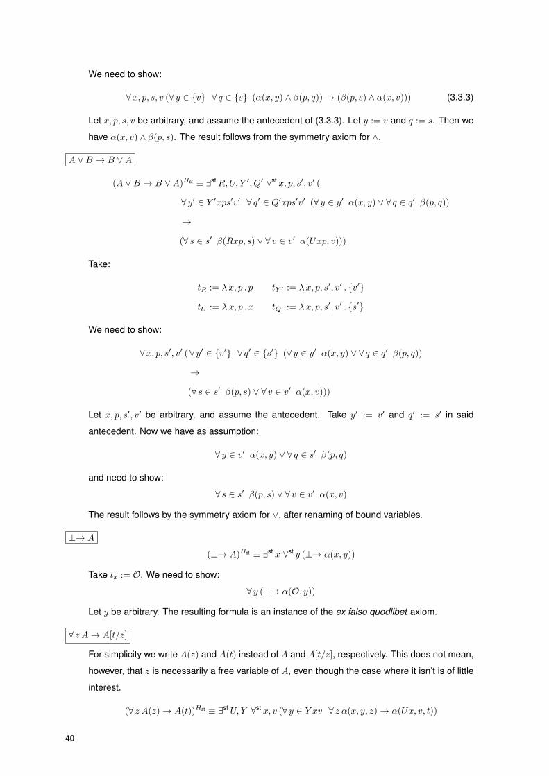
We need to show:
∀x, p, s, v (∀ y ∈ {v} ∀ q ∈ {s} (α(x, y) ∧ β(p, q))→ (β(p, s) ∧ α(x, v))) (3.3.3)
Let x, p, s, v be arbitrary, and assume the antecedent of (3.3.3). Let y := v and q := s. Then we
have α(x, v) ∧ β(p, s). The result follows from the symmetry axiom for ∧.
A ∨B → B ∨A
(A ∨B → B ∨A)Hst ≡ ∃st R,U, Y ′, Q′ ∀st x, p, s′, v′ (
∀ y′ ∈ Y ′xps′v′ ∀ q′ ∈ Q′xps′v′ (∀ y ∈ y′ α(x, y) ∨ ∀ q ∈ q′ β(p, q))
→
(∀ s ∈ s′ β(Rxp, s) ∨ ∀ v ∈ v′ α(Uxp, v)))
Take:
tR := λx, p . p tY ′ := λx, p, s′, v′ . {v′}
tU := λx, p . x tQ′ := λx, p, s′, v′ . {s′}
We need to show:
∀x, p, s′, v′ (∀ y′ ∈ {v′} ∀ q′ ∈ {s′} (∀ y ∈ y′ α(x, y) ∨ ∀ q ∈ q′ β(p, q))
→
(∀ s ∈ s′ β(p, s) ∨ ∀ v ∈ v′ α(x, v)))
Let x, p, s′, v′ be arbitrary, and assume the antecedent. Take y′ := v′ and q′ := s′ in said
antecedent. Now we have as assumption:
∀ y ∈ v′ α(x, y) ∨ ∀ q ∈ s′ β(p, q)
and need to show:
∀ s ∈ s′ β(p, s) ∨ ∀ v ∈ v′ α(x, v)
The result follows by the symmetry axiom for ∨, after renaming of bound variables.
⊥→ A
(⊥→ A)Hst ≡ ∃st x ∀st y (⊥→ α(x, y))
Take tx := O. We need to show:
∀ y (⊥→ α(O, y))
Let y be arbitrary. The resulting formula is an instance of the ex falso quodlibet axiom.
∀ z A→ A[t/z]
For simplicity we write A(z) and A(t) instead of A and A[t/z], respectively. This does not mean,
however, that z is necessarily a free variable of A, even though the case where it isn’t is of little
interest.
(∀ z A(z)→ A(t))Hst ≡ ∃st U, Y ∀st x, v (∀ y ∈ Y xv ∀ z α(x, y, z)→ α(Ux, v, t))
40

Take tU := λx . x and tY := λx, v . {v}. We need to show:
∀x, v (∀ y ∈ {v} ∀ z α(x, y, z)→ α(x, v, t))
Let x, v be arbitrary and assume the antecedent. Then, with y := v, we get ∀ z α(x, v, z). Instan-
tiating z := t, we obtain α(x, v, t), as desired.
A[t/z]→ ∃ z A
As before, we write A(t) and A(z) for A[t/z] and A, respectively.
(A[t/z]→ ∃ z A)Hst ≡ ∃st U, Y ∀st x, v′ (∀ y ∈ Y xv′ α(x, y, t)→ ∃ z ∀ v ∈ v′ α(Ux, v, z))
Take tU := λx . x and tY := λx, v′ . v′. We need to show:
∀x, v′ (∀ y ∈ v′ α(x, y, t)→ ∃ z ∀ v ∈ v′ α(x, v, z))
Let x, v′ be arbitrary. The resulting formula is an instance of the axiom under consideration, after
renaming of a bound variable.
Modus ponensA A→ B
B
By induction hypothesis, we know closed terms t1, t2 and t3 such that:
∀ y α(t1, y) (3.3.4)
∀x, q (∀ y ∈ t2xq α(x, y)→ β(t3x, q)) (3.3.5)
We want to find a closed term tp such that ∀ q β(tp, q). Take tp := t3t1.
Let q be arbitrary. Instantiate x := t1 and q := q in (3.3.5). The goal is now to show the premise
of (3.3.5), which allows us to conclude β(t3t1, q), as desired. Let y ∈ t2t1q be arbitrary. Then by
(3.3.4) with y := y, we get α(t1, y), which is precisely what was needed.
SyllogismA→ B B → C
A→ C
By induction hypothesis, we know closed terms t1, t2, t3 and t4 such that:
∀x, q (∀ y ∈ t1xq α(x, y)→ β(t2x, q)) (3.3.6)
∀ p, w (∀ q ∈ t3pw β(p, q)→ γ(t4p, w)) (3.3.7)
We want to find closed terms tY and tZ such that:
∀x,w (∀ y ∈ tY xw α(x, y)→ γ(tZx,w)) (3.3.8)
Take tY := λx,w .⋃v∈t3(t2x)w t1xv and tZ := λx . t4(t2x). Let x,w be arbitrary and assume the
antecedent of (3.3.8):
∀ y ∈⋃v∈t3(t2x)w t1xv α(x, y) (3.3.9)
41

From (3.3.7) with p := t2x and w := w we get:
∀ q ∈ t3(t2x)w β(t2x, q)→ γ(t4(t2x), w) (3.3.10)
which means that the goal now is to show the antecedent of (3.3.10). Let q0 ∈ t3(t2x)w be
arbitrary. From (3.3.6) with x := x and q := q0 we get:
∀ y ∈ t1xq0 α(x, y)→ β(t2x, q0) (3.3.11)
so it only remains to show the antecedent of (3.3.11). Let y0 ∈ t1xq0 be arbitrary. Since q0 ∈
t3(t2x)w, it follows from Lemma 3.1.7.3 that y0 ∈⋃v∈t3(t2x)w t1xv. Then by (3.3.9) we are done.
Exportation and ImportationA ∧B → C
A→ B → C
A→ B → C
A ∧B → C
(A ∧B → C)Hst ↔
↔ ∃st Z, Y,Q ∀st x, p, w (∀ y ∈ Y xpw α(x, y) ∧ ∀ q ∈ Qxpw β(p, q)→ γ(Zxp,w))
(A→ B → C)Hst ≡
≡ ∃st Z,Q, Y ∀st x, p, w (∀ y ∈ Y xpw α(x, y)→ ∀ q ∈ Qxpw β(p, q)→ γ(Zxp,w))
For both the exportation and importation rules, the terms we get as induction hypothesis from
the premise of the rule do the job for the conclusion.
ExpansionA→ B
C ∨A→ C ∨BBy induction hypothesis, we have closed terms t1 and t2 such that:
∀x, q (∀ y ∈ t1xq α(x, y)→ β(t2x, q)) (3.3.12)
We want to find closed terms tF , tP , tW ′ and tY ′ such that:
∀ z, x, g′, q′ (∀w′ ∈ tW ′zxg′q′ ∀ y′ ∈ tY ′zxg′q′ (∀w ∈ w′ γ(z, w) ∨ ∀ y ∈ y′ α(x, y))
→
∀ g ∈ g′ γ(tF zx, g) ∨ ∀ q ∈ q′ β(tP zx, q))
Take:
tF := λ z, x . z tW ′ := λ z, x, g′, q′ . {g′}
tP := λ z, x . t2x tY ′ := λ z, x, g′, q′ . {⋃q∈q′ t1xq}
We need to show:
∀ z, x, g′, q′ (∀w′ ∈ {g′} ∀ y′ ∈ {⋃q∈q′ t1xq} (∀w ∈ w′ γ(z, w) ∨ ∀ y ∈ y′ α(x, y))
→
∀ g ∈ g′ γ(z, g) ∨ ∀ q ∈ q′ β(t2x, q))
42

Let z, x, g′, q′ be arbitrary and assume the antecedent. Take w′ := g′ and y′ :=⋃q∈q′ t1xq. There
are two cases to consider: if ∀w ∈ g′ γ(z, w), we are done; if not, then we get:
∀ y ∈⋃q∈q′ t1xq α(x, y) (3.3.13)
Let q ∈ q′ be arbitrary. We need to show β(t2x, q). This is a consequence of (3.3.12) with x := x
and q := q, as long as we can prove the antecedent ∀ y ∈ t1xq α(x, y). But by Lemma 3.1.10.3,
t1xq ⊆⋃q∈q′ t1xq, so by (3.3.13) we are done.
∀-introductionB → A
B → ∀ z A, z 6∈ fv(B)
By induction hypothesis, we have closed terms t1 and t2 such that:
∀ p, y (∀ q ∈ t1py β(p, q)→ α(t2p, y)) (3.3.14)
We want to find closed terms tQ and tX such that:
∀ p, y (∀ q ∈ tQpy β(p, q)→ ∀ z α(tXp, y))
Take tQ := t1 and tX := t2. By (3.3.14) and the ∀-introduction rule (z cannot be free in ∀ q ∈
t1py β(p, q) because t1 is closed) it is easy to see that these work.
∃-introductionA→ B
∃ z A→ B, z 6∈ fv(B)
By induction hypothesis there are closed terms t1 and t2 such that:
∀x, q (∀ y ∈ t1xq α(x, y, z)→ β(t2x, q)) (3.3.15)
We want to find closed terms tY ′ and tP such that:
∀x, q (∀ y′ ∈ tY ′xq ∃ z ∀ y ∈ y′ α(x, y, z)→ β(tPx, q))
Take tY ′ := λx, q . {t1xq} and tP := t2. We need to show:
∀x, q (∀ y′ ∈ {t1xq} ∃ z ∀ y ∈ y′ α(x, y, z)→ β(t2x, q)) (3.3.16)
Notice that to show (3.3.16), it is enough to show:
∀x, q ∃ y′ ∈ {t1xq} (∃ z ∀ y ∈ y′ α(x, y, z)→ β(t2x, q)) (3.3.17)
Taking x, q as arbitrary and y′ := t1xq in (3.3.17), it remains to show:
∃ z ∀ y ∈ t1xq α(x, y, z)→ β(t2x, q)
which is a consequence of (3.3.15) with x := x and q := q by the ∃-introduction rule.
43

External induction
Instead of interpreting the external induction axiom, we interpret the equivalent rule, which is
simpler:A(0) ∀st n0 (A(n)→ A(Sn))
∀st n0A(n)
By induction hypothesis, there are closed terms t1, t2 and t3 such that:
∀ y α(t1, y, 0) (3.3.18)
∀n0, x, v (∀ y ∈ t2nxv α(x, y, n)→ α(t3nx, v, Sn)) (3.3.19)
We want a closed term t4 such that:
∀n0, w α(t4n,w, n) (3.3.20)
Take t4 := λn .Rnt1t3. Then, by the defining equations for R, we get:
t40 = t1
t4(Sn) = t3n(t4n)
We prove (3.3.20) by induction on n. The base case with n = 0 is a direct consequence of
(3.3.18). For the step, assume:
∀ y α(t4n, y, n) (3.3.21)
We need to show:
∀wα(t3n(t4n), w, Sn)
Let w be arbitrary. From (3.3.19) with n := n, x := t4n and v := w, we obtain:
∀ y ∈ t2n(t4n)w α(t4n, y, n)→ α(t3n(t4n), w, Sn) (3.3.22)
Observing that (3.3.21) is stronger than the antecedent of (3.3.22), we can conclude the conse-
quent of (3.3.22), which is what we wanted to show in the first place.
∀st z A(z)→ ∀w (stw → A(w))
(∀st z A(z)→ ∀w (stw → A(w)))Hst ≡ ∃st U,Z, Y ∀st X,w′, v (
∀ z ∈ ZXw′v ∀ y ∈ Y Xw′v α(Xz, y, z)→ ∀w ∈ w′ α(UXw′, v, w))
Take:
tU := λX,w′ .⊔z∈w′ Xz
tZ := λX,w′, v . w′
tY := λX,w′, v . {v}
We need to show:
∀X,w′, v (∀ z ∈ w′ ∀ y ∈ {v} α(Xz, y, z)→ ∀w ∈ w′ α(⊔z∈w′ Xz, v, w))
44

Let X,w′, v be arbitrary, and assume the antecedent:
∀ z ∈ w′ ∀ y ∈ {v} α(Xz, y, z) (3.3.23)
We need to show:
∀w ∈ w′ α(⊔z∈w′ Xz, v, w)
Let w ∈ w′ be arbitrary. From (3.3.23) with z := w and y := v, we get α(Xw, v, w). Since w ∈ w′,
we know Xw v⊔z∈w′ Xz by Lemma 3.1.16.2. Then by monotonicity of α, we are done.
∀w (stw → A(w))→ ∀st z A(z)
(∀w (stw → A(w))→ ∀st z A(z))Hst ≡ ∃st X,W ′, V ∀st U, z, y (
∀w′ ∈W ′Uzy ∀ v ∈ V Uzy ∀w ∈ w′ α(Uw′, v, w)→ α(XUz, y, z))
Take:
tX := λU, z . U{z}
tW ′ := λU, z, y . {{z}}
tV := λU, z, y . {y}
We want to show:
∀U, z, y (∀w′ ∈ {{z}} ∀ v ∈ {y} ∀w ∈ w′ α(Uw′, v, w)→ α(U{z}, y, z))
Let U, z, y be arbitrary, and assume the antecedent. From the antecedent, take w′ := {z} and
v := y. So we get ∀w ∈ {z} α(U{z}, y, w) as assumption. Letting w := z, we obtain the desired
result.
∃st z A(z)→ ∃w (stw ∧A(w))
(∃st z A(z)→ ∃w (stw ∧A(w)))Hst ↔ ∃st W ′, U, Y ′ ∀st x, z′, v′ (
∀ y′ ∈ Y ′xz′v′ ∃ z ∈ z′ ∀ y ∈ y′ α(x, y, z)→ ∃w ∈W ′xz′ ∀ v ∈ v′ α(Uxz′, v, w))
Take tW ′ := λx, z′ . z′, tU := λx, z′ . x and tY ′ := λx, z′, v′ . {v′}. We want to show:
∀x, z′, v′ (∀ y′ ∈ {v′} ∃ z ∈ z′ ∀ y ∈ y′ α(x, y, z)→ ∃w ∈ z′ ∀ v ∈ v′ α(x, v, w))
Let x, z′, v′ be arbitrary, and assume the antecedent. Take y′ := v′. Then we have as assump-
tion:
∃ z ∈ z′ ∀ y ∈ v′ α(x, y, z)
and need to show:
∃w ∈ z′ ∀ v ∈ v′ α(x, v, w)
which are the same formulas, after renaming of bound variables.
45

∃w (stw ∧A(w))→ ∃st z A(z)
(∃w (stw ∧A(w))→ ∃st z A(z))Hst ↔ ∃st X,Z ′, V ′ ∀st w′, u, y′ (
∀ v′ ∈ V ′w′uy′ ∃w ∈ w′ ∀ v ∈ v′ α(u, v, w)→ ∃ z ∈ Z ′w′u ∀ y ∈ y′ α(Xw′u, y, z))
Take tX := λw′, u . u, tZ′ := λw′, u . w′ and tV ′ := λw′, u, y′ . {y′}. We want to show:
∀w′, u, y′ (∀ v′ ∈ {y′} ∃w ∈ w′ ∀ v ∈ v′ α(u, v, w)→ ∃ z ∈ w′ ∀ y ∈ y′ α(u, y, z))
Let w′, u, y′ be arbitrary and take v′ := y′. We have as assumption:
∃w ∈ w′ ∀ v ∈ y′ α(u, v, w)
and need to show:
∃ z ∈ w′ ∀ y ∈ y′ α(u, y, z)
which are the same formulas, after renaming of bound variables.
st z ∧ z = w → stw
(st z ∧ z = w → stw)Hst ≡ ∃st W ′ ∀st z′ (z ∈ z′ ∧ z = w → w ∈W ′z′)
Take tW ′ := λ z′ . z′. We need to show:
∀ z′ (z ∈ z′ ∧ z = w → w ∈ z′)
which is a consequence of Proposition 3.1.1.
stu, u closed
(stu)Hst ≡ ∃st u′ (u ∈ u′)
Take tu′ := {u}. We need to show u ∈ {u}, which is an instance of Lemma 3.1.7.1. Note that u
needs to be closed, otherwise {u} wouldn’t be closed, as is required.
st f ∧ st z → st(fz)
(st f ∧ st z → st(fz))Hst ≡ ∃st U ∀st f ′, z′ (f ∈ f ′ ∧ z ∈ z′ → fz ∈ Uf ′z′)
Take:
tU := λ f ′, z′ .⋃f∈f ′
⋃z∈z′ fz
We need to show:
∀ f ′, z′ (f ∈ f ′ ∧ z ∈ z′ → fz ∈⋃f∈f ′
⋃z∈z′ fz)
which is a consequence of Lemma 3.1.7.3.
Internal axioms
From Lemma 3.3.2, the Hst-interpretation of internal formulas leaves them unchanged. This
means that this result follows trivially for such formulas. The internal axioms that get taken care
of are the equality axioms, the axiom of internal induction, the axioms for S, for Π, for Σ, for R,
and for L, and the sequence axiom.
46

Iω
Recall that, in the following, z′ and u represent tuples of variables. Using Lemma 3.3.2.2:
(∀st z′ ∃w ∀ z ∈ z′ ϕ(z, w)→ ∃ v ∀st uϕ(u, v))Hst ↔
↔ ∃st Z ′ ∀st u′ (∀ z′ ∈ Z ′u′ ∃w ∀ z ∈ z′ ϕ(z, w)→ ∃ v ∀u ∈ u′ ϕ(u, v))
Take tZ′ := λu′ . {u′}. We need to show:
∀u′ (∀ z′ ∈ {u′} ∃w ∀ z ∈ z′ ϕ(z, w)→ ∃ v ∀u ∈ u′ ϕ(u, v)) (3.3.24)
Let u′ be arbitrary, and assume the antecedent of (3.3.24). Let z′ := u′. We get
∃w ∀ z ∈ u′ ϕ(z, w)
which is precisely what we wanted, after renaming of bound variables.
NCRω
(∀w ∃st z A(z, w)→ ∃st s′ ∀ r ∃ s ∈ s′ A(s, r))Hst ↔
↔ ∃st U, S′′, Y ′ ∀st x, z′, v′′ (
∀ y′ ∈ Y ′xz′v′′ ∀w ∃ z ∈ z′ ∀ y ∈ y′ α(x, y, z, w)
→
∃ s′ ∈ S′′xz′ ∀ v′ ∈ v′′ ∀ r ∃ s ∈ s′ ∀ v ∈ v′ α(Uxz′, v, s, r))
Take tU := λx, z′ . x, tS′′ := λx, z′ . {z′} and tY ′ := λx, z′, v′′ . v′′. We need to show:
∀x, z′, v′′ (∀ y′ ∈ v′′ ∀w ∃ z ∈ z′ ∀ y ∈ y′ α(x, y, z, w)
→
∃ s′ ∈ {z′} ∀ v′ ∈ v′′ ∀ r ∃ s ∈ s′ ∀ v ∈ v′ α(x, v, s, r))
Let z, x′, v′′ be arbitrary, and assume the antecedent. Take s′ := z′ in the consequent. So
currently we have as assumption:
∀ y′ ∈ v′′ ∀w ∃ z ∈ z′ ∀ y ∈ y′ α(x, y, z, w)
and need to show:
∀ v′ ∈ v′′ ∀ r ∃ s ∈ z′ ∀ v ∈ v′ α(x, v, s, r)
These are the same formulas, after renaming of bound variables.
HACω
(∀st z ∃st wA(z, w)→ ∃st S ∀st r ∃ s ∈ Sr A(r, s))Hst ↔
↔ ∃st U ,S ′, Z, Y ′ ∀st X,W ′, r′, v′′ (
∀ z ∈ ZXW ′r′v′′ ∀ y′ ∈ Y ′XW ′r′v′′ ∃w ∈W ′z ∀ y ∈ y′ α(Xz, y, z, w)
→
∃S ∈ S ′XW ′ ∀ r ∈ r′ ∀ v′ ∈ v′′ ∃ s ∈ Sr ∀ v ∈ v′ α(UXW ′r, v, r, s))
47

Take:
tU := λX,W ′ . X tZ := λX,W ′, r′, v′′ . r′
tS′ := λX,W ′ . {W ′} tY ′ := λX,W ′, r′, v′′ . v′′
We need to show:
∀X,W ′, r′, v′′ (∀ z ∈ r′ ∀ y′ ∈ v′′ ∃w ∈W ′z ∀ y ∈ y′ α(Xz, y, z, w)
→
∃S ∈ {W ′} ∀ r ∈ r′ ∀ v′ ∈ v′′ ∃ s ∈ Sr ∀ v ∈ v′ α(Xr, v, r, s))
Let X,W ′, r′, v′′ be arbitrary, and assume the antecedent. Take S := W ′ in the consequent. So
we currently have as assumption:
∀ z ∈ r′ ∀ y′ ∈ v′′ ∃w ∈W ′z ∀ y ∈ y′ α(Xz, y, z, w)
and need to show:
∀ r ∈ r′ ∀ v′ ∈ v′′ ∃ s ∈W ′r ∀ v ∈ v′ α(Xr, v, r, s)
These are exactly the same formulas, after renaming of bound variables.
HGMPωst
((∀st z ϕ(z)→ ψ)→ ∃st w′ (∀w ∈ w′ ϕ(w)→ ψ))Hst ≡
≡ ∃st W ′′ ∀st z′ ((∀ z ∈ z′ ϕ(z)→ ψ)→ ∃w′ ∈W ′′z′ (∀w ∈ w′ ϕ(w)→ ψ))
Take tW ′′ := λ z′ . {z′}. We need to show:
∀ z′ ((∀ z ∈ z′ ϕ(z)→ ψ)→ ∃w′ ∈ {z′} (∀w ∈ w′ ϕ(w)→ ψ))
Let z′ be arbitrary, and assume the antecedent. Take w′ := z′ in the consequent. We currently
have as assumption:
∀ z ∈ z′ ϕ(z)→ ψ
and want to show:
∀w ∈ z′ ϕ(w)→ ψ
These are the same formulas, after renaming of a bound variable.
HIPω∀st
((∀st z ϕ(z)→ ∃st wA(w))→ ∃st s′ (∀st r ϕ(r)→ ∃ s ∈ s′ A(s)))Hst ↔
↔ ∃st U,R, S′′, Y ′ ∀st x,w′, Z, v′′ (
∀ y′ ∈ Y ′xw′Zv′′ (∀ z ∈ Zy′ ϕ(z)→ ∃w ∈ w′ ∀ y ∈ y′ α(x, y, w))
→
∃ s′ ∈ S′′xw′Z ∀ v′ ∈ v′′ (∀ r ∈ Rxw′Zv′ ϕ(r)→ ∃ s ∈ s′ ∀ v ∈ v′ α(Uxw′Z, v, s)))
48
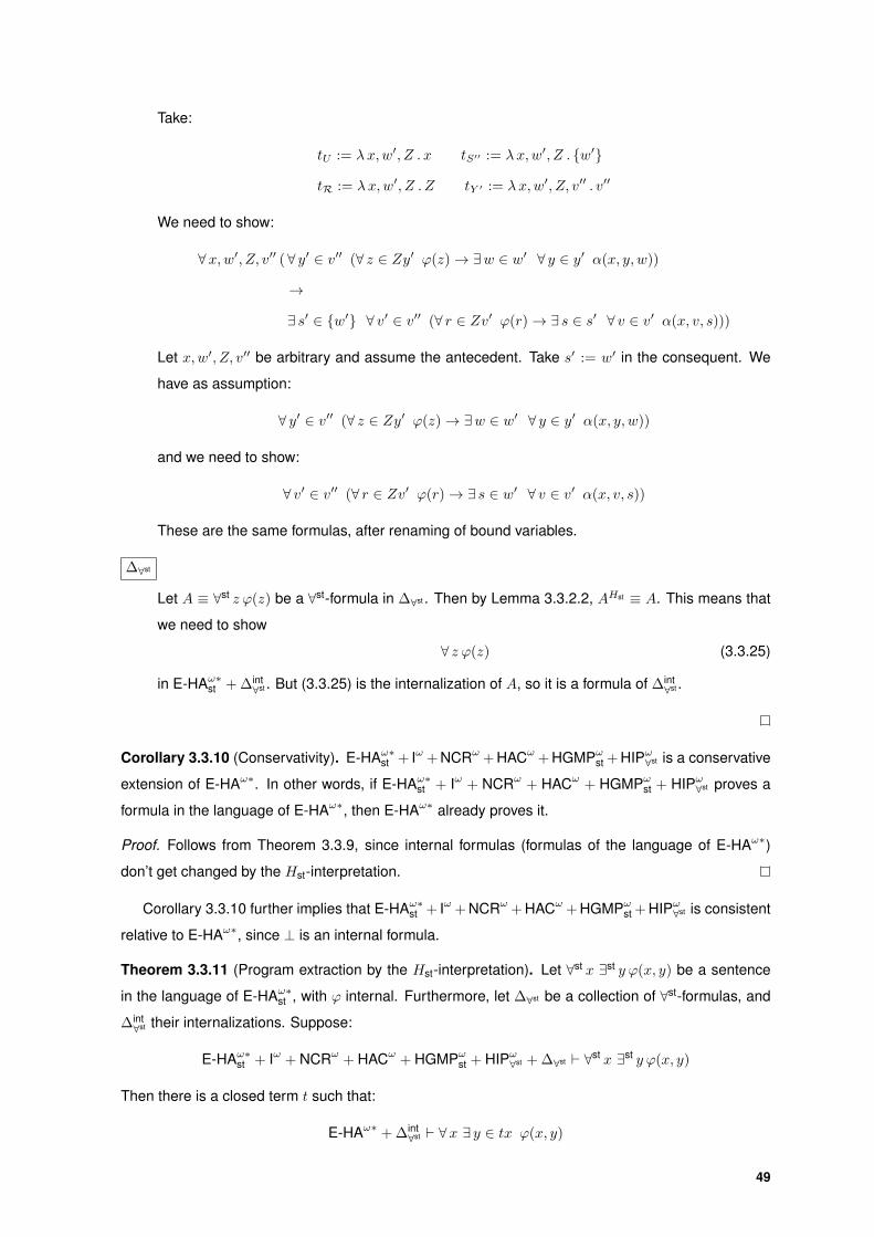
Take:
tU := λx,w′, Z . x tS′′ := λx,w′, Z . {w′}
tR := λx,w′, Z . Z tY ′ := λx,w′, Z, v′′ . v′′
We need to show:
∀x,w′, Z, v′′ (∀ y′ ∈ v′′ (∀ z ∈ Zy′ ϕ(z)→ ∃w ∈ w′ ∀ y ∈ y′ α(x, y, w))
→
∃ s′ ∈ {w′} ∀ v′ ∈ v′′ (∀ r ∈ Zv′ ϕ(r)→ ∃ s ∈ s′ ∀ v ∈ v′ α(x, v, s)))
Let x,w′, Z, v′′ be arbitrary and assume the antecedent. Take s′ := w′ in the consequent. We
have as assumption:
∀ y′ ∈ v′′ (∀ z ∈ Zy′ ϕ(z)→ ∃w ∈ w′ ∀ y ∈ y′ α(x, y, w))
and we need to show:
∀ v′ ∈ v′′ (∀ r ∈ Zv′ ϕ(r)→ ∃ s ∈ w′ ∀ v ∈ v′ α(x, v, s))
These are the same formulas, after renaming of bound variables.
∆∀st
Let A ≡ ∀st z ϕ(z) be a ∀st-formula in ∆∀st . Then by Lemma 3.3.2.2, AHst ≡ A. This means that
we need to show
∀ z ϕ(z) (3.3.25)
in E-HAω∗st + ∆int∀st . But (3.3.25) is the internalization of A, so it is a formula of ∆int
∀st .
Corollary 3.3.10 (Conservativity). E-HAω∗st + Iω + NCRω + HACω + HGMPωst + HIPω∀st is a conservative
extension of E-HAω∗. In other words, if E-HAω∗st + Iω + NCRω + HACω + HGMPωst + HIPω∀st proves a
formula in the language of E-HAω∗, then E-HAω∗ already proves it.
Proof. Follows from Theorem 3.3.9, since internal formulas (formulas of the language of E-HAω∗)
don’t get changed by the Hst-interpretation.
Corollary 3.3.10 further implies that E-HAω∗st + Iω + NCRω + HACω + HGMPωst + HIPω∀st is consistent
relative to E-HAω∗, since ⊥ is an internal formula.
Theorem 3.3.11 (Program extraction by the Hst-interpretation). Let ∀st x ∃st y ϕ(x, y) be a sentence
in the language of E-HAω∗st , with ϕ internal. Furthermore, let ∆∀st be a collection of ∀st-formulas, and
∆int∀st their internalizations. Suppose:
E-HAω∗st + Iω + NCRω + HACω + HGMPωst + HIPω∀st + ∆∀st ` ∀st x ∃st y ϕ(x, y)
Then there is a closed term t such that:
E-HAω∗ + ∆int∀st ` ∀x ∃ y ∈ tx ϕ(x, y)
49

Proof. Direct consequence of Theorem 3.3.9, taking into account that:
(∀st x ∃st y ϕ(x, y))Hst ≡ ∃st Y ∀st x ∃ y ∈ Y x ϕ(x, y)
Theorem 3.3.12 (Characterization theorem for the Hst-interpretation). For all formulas of the lan-
guage of E-HAω∗st :
E-HAω∗st + Iω + NCRω + HACω + HGMPωst + HIPω∀st ` A↔ AHst
Proof. By induction on the logical structure of A.
Internal atomic formulas
For an internal atomic formula ϕ, ϕHst ≡ ϕ, so there is nothing to show.
st z
(st z)Hst ≡ ∃st z′ (z ∈ z′)
To show st z → ∃st z′ (z ∈ z′), take z′ := {z}. This is a standard term by Remark 3.1.22, and
does the job by Lemma 3.1.7.1.
The other implication, ∃st z′ (z ∈ z′)→ st z, results from Lemma 3.1.24.
For the steps of the induction dealing with formulas A and B, we follow [2] in noting that, according
to Section 1.6.17 of [43], there are internal formulas α and β such that E-HAω∗st proves:
AHst ↔ ∃st x ∀st y α(x, y) and BHst ↔ ∃st u ∀st v β(u, v)
These formulas are obtained through embeddings of tuples of types in a higher type, and coding with
inverses of tuples of terms in a single term.
With this in mind, we can take the tuples of variables given by the Hst-interpretation as a single
variable.
A ∧B
Since by induction hypothesis A↔ AHst and B ↔ BHst , it suffices to show
AHst ∧BHst ↔ (A ∧B)Hst
∃st x ∀st y α(x, y) ∧ ∃st u ∀st v β(u, v)↔ ∃st x, u ∀st y, v (α(x, y) ∧ β(u, v))
which is straightforward in E-HAω∗st .
A ∨B
We need to show:
AHst ∨BHst ↔ (A ∨B)Hst
∃st x ∀st y α(x, y) ∨ ∃st u ∀st v β(u, v)↔ ∃st x, u ∀st y′, v′ (∀ y ∈ y′ α(x, y) ∨ ∀ v ∈ v′ β(u, v))
From left to right, this is straightforward in E-HAω∗st . From right to left we need LLPOωst, which is
a consequence of Iω by Lemma 3.2.11.
50

A→ B
Consider the following enumeration of formulas, starting with AHst → BHst and ending with
(A→ B)Hst :
(1) ∃st x ∀st y α(x, y)→ ∃st u ∀st v β(u, v)
(2) ∀st x (∀st y α(x, y)→ ∃st u ∀st v β(u, v))
(3) ∀st x ∃st u (∀st y α(x, y)→ ∀st v β(u, v))
(4) ∀st x ∃st u ∀st v (∀st y α(x, y)→ β(u, v))
(5) ∀st x ∃st u ∀st v ∃st y′ (∀ y ∈ y′ α(x, y)→ β(u, v))
(6) ∃st U ∀st x ∀st v ∃st y′ (∀ y ∈ y′ α(x, y)→ β(Ux, v))
(7) ∃st U ∀st x ∃st Y ∀st v (∀ y ∈ Y v α(x, y)→ β(Ux, v))
(8) ∃st U,Y ∀st x, v (∀ y ∈ Yxv α(x, y)→ β(Ux, v))
Clearly it suffices to show (i) ↔ (i + 1) for all i ∈ {1, . . . , 7}. All the implications (i + 1) → (i)
are easily provable in E-HAω∗st (Lemma 3.1.24 is necessary for (5) → (4)). The implications
(1)→ (2) and (3)→ (4) only need E-HAω∗st as well.
The implication (2) → (3) is a consequence of HIPω∀st , taking into account that ∀st v β(u, v) is
monotone on u, and (4)→ (5) comes form HGMPωst.
As for the remaining three implications, they all follow from HACω and the following facts:
• ∀st v ∃st y′ (∀ y ∈ y′ α(x, y)→ β(u, v)) is monotone on u, consequence of the monotonicity
of β on the same variable;
• ∀ y ∈ y′ α(x, y)→ β(Ux, v) is monotone on y′, consequence of Lemma 3.1.10.1;
• ∀st v (∀ y ∈ Y v α(x, y) → β(Ux, v)) is monotone on Y , again consequence of Lemma
3.1.10.1.
∀ z A(z)
We need to show:
∀ z A(z)Hst ↔ (∀ z A(z))Hst
∀ z ∃st x ∀st xα(x, y, z)↔ ∃st x ∀st y ∀ z α(x, y, z)
From left to right we use the monotonicity of ∀st y α(x, y, z) on x, and NCRω. From right to left
E-HAω∗st suffices.
∃ z A(z)
We need to show:
∃ z A(z)Hst ↔ (∃ z A(z))Hst
∃ z ∃st x ∀st y α(x, y, z)↔ ∃st x ∀st y′ ∃ z ∀ y ∈ y′ α(x, y, z)
From left to right E-HAω∗st is enough (using Lemma 3.1.24). From right to left we use Iω.
51

∀st z A(z)
We need to show:
∀st z A(z)Hst ↔ (∀st z A(z))Hst
∀st z ∃st x ∀st y α(x, y, z)↔ ∃st X ∀st z, y α(Xz, y, z)
From left to right we use HACω and the monotonicity of ∀st y α(x, y, z) on x. From right to left
E-HAω∗st suffices.
∃st z A(z)
We need to show:
∃st z A(z)Hst ↔ (∃st z A(z))Hst
∃st z ∃st x ∀st y α(x, y, z)↔ ∃st z′, x ∀st y′ ∃ z ∈ z′ ∀ y ∈ y′ α(x, y, z)
Similarly to the case for ∃, from left to right we use Lemma 3.1.24 and from right to left, the
principle Iω.
We can prove that there are no characteristic principles missing in the statement of the soundness
theorem for the Hst-interpretation (Theorem 3.3.9):
Theorem 3.3.13. Let H := E-HAω∗st + Iω + NCRω + HACω + HGMPωst + HIPω∀st be the theory in which
we can prove the characterization theorem for the Hst-interpretation.
Let C be a characteristic principle, i.e., a principle for which it is possible to prove that for every
formula A of the language of E-HAω∗st with AHst ≡ ∃st x ∀st y αHst(x,y), if
H + C ` A
then there are closed terms of the language of E-HAω∗ such that
E-HAω∗ ` ∀y αHst(t,y).
Then C is already provable from H.
Proof. Let CHst ≡ ∀st x ∃st y γHst(x,y). Since clearly H +C ` C, we know that there are closed terms
t such that:
E-HAω∗ ` ∀y γHst(t,y)
Then E-HAω∗st proves the same statement. In particular:
E-HAω∗st ` ∀st y γHst(t,y)
which is a weaker statement. Now, since the terms t are closed, they are standard, and hence:
E-HAω∗st ` ∃st x ∀st y γHst(x,y)
E-HAω∗st ` CHst
52

Now since the theory H is stronger than E-HAω∗st , we also have H ` CHst , and by the characterization
theorem (Theorem 3.3.12), H ` C as we wanted to show.
From the characterization theorems of the Hst-interpretation (Theorem 3.3.12) and of the Dst-
interpretation presented in [2], we get:
Theorem 3.3.14. For all formulas A of the language of E-HAω∗st :
E-HAω∗st + Iω + NCRω + HACω + HGMPωst + HIPω∀st ` AHst ↔ ADst
As is the case with the dialectica interpretation of Godel, the Hst-interpretation could be coupled
with a negative translation to bring it into the realm of Peano arithmetic. It would be interesting to find
the negative translation that would produce the Sst-interpretation defined below, in the same spirit as
Streicher and Kohlenbach did for the interpretations of Godel and Shoenfield in [41]. In fact, in [2] Van
den Berg et al. did just that for their interpretations, which are very similar to the ones described in
this thesis.
3.4 The Sst-interpretation
The Sst-interpretation is an interpretation of classical nonstandard arithmetic based on Shoen-
field’s interpretation (outlined in Section 2.3). It was proposed in its first version by Van den Berg,
Briseid, and Safarik in [2]. Later it was slightly modified by Dinis and Ferreira in [10]. In their paper,
Dinis and Ferreira consider a weaker theory than E-PAω∗st , namely E-PRAω∗st , where the only recur-
sor available is of type 0, and induction is restricted to quantifier-free formulas. The version here
presented is an extension of Dinis and Ferreira’s Sst-interpretation to E-PAω∗st .
Definition 3.4.1 (Sst-interpretation). The Sst-interpretation associates to each formula A of the lan-
guage of E-PAω∗st a formula ASst of the form:
ASst ≡ ∀st x ∃st y αSst(x,y)
with the same free variables and in the same language as A. The (possibly empty) variable tuples x
and y and their types are uniquely determined by the logical structure of A. It is important that these
variables do not appear free in A. Furthermore, αSst is an internal formula.
The definition proper is given below. The sub-formulas inside square brackets are the internal
formulas corresponding to αSst above.
• αSst :≡ αSst :≡ α for internal atomic formulas α
• (st z)Sst :≡ ∃st z′ [z ∈ z′]
Given the interpretations ASst ≡ ∀st x ∃st y αSst(x,y) and BSst ≡ ∀st u ∃st v βSst(u,v):
• (A ∨B)Sst :≡ ∀st x,u ∃st y,v [αSst(x,y) ∨ βSst(u,v)]
• (¬A)Sst :≡ ∀st Y ∃st x′ [∃x ∈ x′ ¬αSst(x,Y x)]
53

• (∀ z A(z))Sst :≡ ∀st x ∃st y [∀ z αSst(x,y, z)]
Remark 3.4.2. Internal formulas remain unchanged after the Sst-interpretation.
Lemma 3.4.3. Let A be an arbitrary formula of the language of E-PAω∗st such that
ASst ≡ ∀st x ∃st y α(x,y)
Then y is of star type and α is monotone on y.
Idea of Proof. Straightforward induction on the logical structure of A.
Definition 3.4.4 (HACωint). The herbrandised schema of choice for internal formulas, HACωint, is the
union for all types ρ, τ of:
HACρ,τint : ∀st zρ ∃st wτ ϕ(z, w)→ ∃st W ′ρ→τ∗∀st zρ ∃w ∈W ′z ϕ(z, w)
where ϕ is any internal formula in the language of E-PAω∗.
Theorem 3.4.5 (Soundness of the Sst-interpretation). Let A be an arbitrary formula in the language
of E-PAω∗st , possibly with free variables, such that ASst ≡ ∀st x ∃st y αSst(x,y). Furthermore, let ∆int be
a collection of internal formulas. Suppose:
E-PAω∗st + Iω + HACωint + ∆int ` A
Then there are closed terms t, which can be extracted from a proof of A, such that:
E-PAω∗ + ∆int ` ∀xαSst(x, tx)
Idea of Proof. By induction on the derivation of A, using the monotonicity of αSst in the existentially
quantified variables. The proof can be found in [10]. Even though they use a weaker theory than here,
namely E-PRAω∗st , the only extra axiom that we need to check is external induction. For convenience,
we interpret the external induction rule, which is equivalent, instead:
A(0) ∀st n0 (A(n)→ A(Sn))
∀st n0A(n)
Suppose A(n)Sst ≡ ∀st xρ ∃st yτ∗α(x, y, n) where x, y should be thought of as tuples of variables.
During the rest of this proof we discard the tuple notation for simplicity.
By induction hypothesis, there are closed terms Y of type ρ → τ∗, U ′ of type 0∗ → (ρ → τ∗) →
ρ→ ρ∗, and Q of type 0∗ → (ρ→ τ∗)→ ρ→ τ∗ such that:
∀xα(x, Y x, 0) (3.4.1)
∀n′0∗, V, p ∀n ∈ n′ (∀u ∈ U ′n′V p α(u, V u, n)→ α(p,Qn′V p, Sn)) (3.4.2)
And we need to find a closed term W of type 0∗ → ρ→ τ∗ such that:
∀m′0∗, z ∀m ∈ m′ α(z,Wm′z,m) (3.4.3)
We want to use a similar strategy to the one used in the treatment of the external induction rule during
the proof of Theorem 3.3.9. Ideally, the formulas (3.4.2) and (3.4.3) would start with a universal
quantification over a term of type 0, instead of with a universal quantification over a term of type 0∗.
In fact, we can massage said formulas until they are in our preferred form:
54

1. Let U ′ := λn0 . U ′{n} and Q := λn0 . Q{n}. Then from (3.4.2) it is possible to prove:
∀n0, V, p (∀u ∈ U ′nV p α(u, V u, n)→ α(p,QnV p, Sn)) (3.4.4)
2. GivenW of type 0→ ρ→ τ∗ such that
∀m0, z α(z,Wmz,m) (3.4.5)
it is possible to prove (3.4.3) with W := λm′0∗.⊔k∈m′Wk.
Now we can reformulate the goal: from (3.4.1) and (3.4.4), find W of type 0 → ρ → τ∗ such that
(3.4.5).
TakeW := λm0 . RmYQ. From the recursor axioms we get:
W0 = Y
W(Sm) = Qm(Wm)
We show (3.4.5) by induction on m. The base case with m = 0 is a direct consequence of (3.4.1).
For the step, assume:
∀ z α(z,Wmz,m) (3.4.6)
and let z0 be arbitrary. We need to show α(z0,W(Sm)z0, Sm). Unravelling W(Sm), we see that the
goal is really α(z0,Qm(Wm)z0, Sm). So take in (3.4.4) n := m, V :=Wm, p := z0, obtaining:
∀u ∈ U ′m(Wm)z0 α(u,Wmu,m)→ α(z0,Qm(Wm)z0, Sm) (3.4.7)
Noticing that (3.4.6) is stronger than the antecedent of (3.4.7), we can conclude its consequent, which
was precisely our goal.
Theorem 3.4.6 (Characterization theorem for the Sst-interpretation). For all formulas of the language
of E-PAω∗st :
E-PAω∗st + Iω + HACωint ` A↔ ASst
Proof. By induction on the logical structure of A.
Internal atomic formulas
For an internal atomic formula ϕ, ϕSst ≡ ϕ, so there is nothing to show.
st z
Since (st z)Sst ≡ (st z)Hst , this step coincides with the step for st z in the proof of Theorem 3.3.12
(where only E-HAω∗st is used).
As in the proof of Theorem 3.3.12, we note that there are internal formulas α and β such that
E-PAω∗st proves:
ASst ↔ ∀st x ∃st y α(x, y) and BSst ↔ ∀st u ∃st v β(u, v)
and hence can take the tuples of variable given by the Sst-interpretation as a single variable.
55

A ∨B
By induction hypothesis, A↔ ASst and B ↔ BSst , so it suffices to show:
ASst ∨BSst ↔ (A ∨B)Sst
∀st x ∃st y α(x, y) ∨ ∀st u ∃st v β(u, v)↔ ∀st x, u ∃st y, v (α(x, y) ∨ β(u, v))
which easy to check in E-PAω∗st .
¬A
We need to show:
¬ASst ↔ (¬A)Sst
¬∀st x ∃st y α(x, y)↔ ∀st Y ∃st x′ ∃x ∈ x′ ¬α(x, y)
Consider the following:
(1) ¬∀st x ∃st y α(x, y)
(2) ¬∃st Y ′ ∀st x ∃ y ∈ Y ′x α(x, y)
(3) ∀st Y ′ ∃st x ∀ y ∈ Y ′x ¬α(x, y)
(4) ∀st Y ∃st x′ ∃st x ∈ x′ ¬α(x, Y x)
It is enough to show (i)↔ (i+1) for all i ∈ {1, 2, 3}. The implication (1)→ (2) is a consequence
of HACωint. The other side is easy to check in E-PAω∗st , using Lemma 3.1.24. The equivalence
(2)↔ (3) follows from the rules for negation. For (3)→ (4), take Y ′ := λx . {Y x} and x′ := {x};
the result uses Lemma 3.1.7.1. For (4) → (3), take Y := λx .⋃v∈Y ′x v; the result follows by
Lemmas 3.1.24, 3.1.10.3, and the monotonicity of α(x, y) on y.
∀ z A(z)
We need to show:
∀ z A(z)Sst ↔ (∀ z A(z))Sst
∀ z ∀st x ∃st y α(x, y, z)↔ ∀st x ∃st y ∀ z α(x, y, z)
From right to left this is straightforward in E-PAω∗st . From left to right we use the realization
principle Rω, taking into account that α(x, y, z) is monotone on y. This is possible because Rω
is the contrapositive of Iω.
From the characterization theorems for the Sst-interpretation presented here and Van den Berg et
al.’s interpretation for classical logic presented in [2] (here written as Sst(Berg)) we get:
Theorem 3.4.7. For all formulas A of the language of E-PAω∗st :
E-PAω∗st + Iω + HACωint ` ASst ↔ ASst(Berg)
56

3.5 Countable saturation
In this section, we briefly study the CSATω principle, which is common among nonstandard argu-
ments.
Definition 3.5.1 (CSATω). The countable saturation principle, CSATω, is the union for all types ρ of:
CSATρ : ∀st n0 ∃ zρA(n, z)→ ∃Z0→ρ ∀st n0A(n,Zn)
for all formulas A of the language of E-HAω∗.
We will see that CSATω is interpreted by the Hst-interpretation, or in other words, that it is a
characteristic principle.
The story is different when we’re in a classical setting. Here adding even CSAT0 to E-PAω∗st + OS0
already gives us the strength of full second-order Peano arithmetic. In fact, as is seen by Van den
Berg et al. in [3], E-PAω∗st + Iω + HACωint + CSATω has exactly the strength of second-order arithmetic.
3.5.1 Countable saturation in an intuitionistic setting
We will see that it is possible to reduce theHst-interpretation of CSATω to the finite axiom of choice,
ACωfin. Hence a first goal is to show that E-HAω∗ proves ACωfin.
Definition 3.5.2 (ACωfin). The finite axiom of choice, ACωfin, is the union for all types ρ of:
ACρfin : ∀ s0∗
(∀n ∈ s ∃xρ ϕ(n, x)→ ∃X0→ρ ∀n ∈ s ϕ(n,Xn))
for all formulas ϕ of the language of E-HAω∗.
Lemma 3.5.3. E-HAω∗ ` ACωfin.
Proof. By sequence induction on s0∗. If s = {}, then the consequent of ACωfin is trivially true, since
∀n¬(n ∈ {}).
For a sequence s′ = prep ks we know by induction hypothesis:
∀n ∈ s ∃xϕ(n, x)→ ∃X ∀n ∈ s ϕ(n,Xn) (3.5.1)
Assume:
∀n ∈ prep ks ∃xϕ(n, x) (3.5.2)
From (3.5.2), take n := k and xk such that
ϕ(k, xk) (3.5.3)
Since (3.5.2) is stronger than the antecedent of (3.5.1), we also get its consequent:
∃X ∀n ∈ s ϕ(n,Xn) (3.5.4)
Take X0 such that
∀n ∈ s ϕ(x,X0n) (3.5.5)
57

as in (3.5.4). We are now able to build:
X := λn .
{xk if n =0 k
X0n otherwise
by taking into account the decidability of type 0 equality. It remains to show:
∀n ∈ prep ks ϕ(n,Xn)
If n = k, this follows from (3.5.3). If n ∈ s, it follows from (3.5.5) instead. There are no more cases to
consider.
Theorem 3.5.4. E-HAω∗st + Iω + NCRω + HACω + HGMPωst + HIPω∀st ` CSATω.
Proof. By Theorem 3.3.13, it suffices to extend the proof of the soundness theorem for theHst-interpre-
tation (Theorem 3.3.9) for the CSATω principle.
Let AHst ≡ ∃st x ∀st y α(x, y) where x, y should be regarded as tuples, even though we don’t write
x or y for simplicity.
(∀st n ∃ z A(n, z)→ ∃W ∀st mA(m,Wm))Hst ≡ ∃st U,N, Y ′ ∀st X,m′, v′ (
∀n ∈ NXm′v′ ∀ y′ ∈ Y ′Xm′v′ ∃ z ∀ y ∈ y′ α(Xn, y, n, z)
→
∃W ∀m ∈ m′ ∀ v ∈ v′ α(UXm, v,m,Wm))
Take tU := λX .X, tN := λX,m′, v′ .m′ and tY ′ := λX,m′, v′ . {v′}. We need to show in E-HAω∗:
∀X,m′, v′ (∀n ∈ m′ ∀ y′ ∈ {v′} ∃ z ∀ y ∈ y′ α(Xn, y, n, z)
→
∃W ∀m ∈ m′ ∀ v ∈ v′ α(Xm, v,m,Wm))
or simply:
∀X,m′, v′ (∀n ∈ m′ ∃ z ∀ y ∈ v′ α(Xn, y, n, z)
→
∃W ∀m ∈ m′ ∀ v ∈ v′ α(Xm, v,m,Wm))
which is an instance of ACωfin. So, by Lemma 3.5.3, we are done.
3.5.2 Countable saturation in a classical setting
We now want to show that E-PAω∗st + OS0 + CSAT0 interprets full second-order arithmetic.
Definition 3.5.5 (PA2). Full second-order Peano arithmetic, PA2, is a two-sorted classical system, that
distinguishes between number terms (denoted as lower-case Latin letters) and set terms (denoted
as upper-case Latin letters). The language includes the usual logic connectives (with distinguished
quantifiers for numbers and for sets), the constants 0 and 1 with their usual meanings, the functions
58

+ (sum of two numbers) and · (product of two numbers), and three predicates: = (equality between
numbers), < (inequality between numbers), and ∈ (membership of a number in a set).
Other than logical axioms for classical logic and basic axioms governing the behaviour of the
various terms available, it also includes an induction axiom:
(0 ∈ X ∧ ∀n (n ∈ X → n+ 1 ∈ X))→ ∀n (n ∈ X)
and the full comprehension schema:
∃X ∀n (n ∈ X ↔ ϕ(n))
where ϕ is any formula without X as free variable.
The full definition can be found, for example, in Section I.2 of [39] (where PA2 is named Z2).
Lemma 3.5.6. E-PAω∗st ` ∀st n0 ∀m0 (¬ stm→ n < m).
Proof. It suffices to notice that: either n < m and we are done, or m ≤ n, and then m must be
standard by Lemma 3.1.23.
Theorem 3.5.7. E-PAω∗st + OS0 + CSAT0 interprets PA2.
Proof. The idea is to see number terms of PA2 as standard terms of type 0 in E-PAω∗st and set terms
of PA2 as terms of type 0∗ in E-PAω∗st . Then all the terms of PA2 have ready interpretations in E-PAω∗st .
Classical logic is interpreted, as well as the basic axioms defining the behaviour of the terms of
PA2. For the induction axiom of PA2 we can use the external induction axiom of E-PAω∗st . Now it only
remains to show that full comprehension is verified. Translating this schema into the language of
E-PAω∗st , we need to show that for every formula A:
∃ s0∗∀st n0 (n ∈ s↔ A(n))
We start by noticing that, with the help of the law of excluded middle, E-PAω∗st shows:
∀st n0 ∃ k0 (k = 0↔ A(n)) (3.5.6)
Then from CSAT0 and (3.5.6) we obtain:
∃K0→0 ∀st n0 (Kn = 0↔ A(n)) (3.5.7)
Take K in the circumstances of (3.5.7). It is easy to show by external induction that:
∀st m0 ∃ s0∗
m (∀n ≤ m (n ∈ sm ↔ Kn = 0) ∧ ∀ l ∈ sm (l ≤ m)) (3.5.8)
It suffices to take:
s0 :=
{{0} if K0 =0 0
{} otherwises(Sm) :=
{prep0(Sm)sm if K(Sm) =0 0
sm otherwise
We don’t really care that ∀ l ∈ sm (l ≤ m), but it is easy to show and makes the induction hypotheses
strong enough to prove the other part.
59

From (3.5.8) and OS0 we get:
∃m0 (¬ stm ∧ ∃ s0∗
(∀n ≤ m (n ∈ s↔ Kn = 0) ∧ ∀ l ∈ s (l ≤ m)))
So there is a nonstandard number m for which:
∃ s0∗∀n ≤ m (n ∈ s↔ Kn = 0) (3.5.9)
Since by Lemma 3.5.6 all standard numbers are less than any nonstandard number, from (3.5.9) in
particular:
∃ s0∗∀st n (n ∈ s↔ Kn = 0) (3.5.10)
From (3.5.6) and (3.5.10) we are done:
∃ s0∗∀st n (n ∈ s↔ A(n))
60

4A note on Weihrauch reducibility
Contents4.1 Weihrauch reducibility . . . . . . . . . . . . . . . . . . . . . . . . . . . . . . . . . . 624.2 A comment on how to use the dialectica interpretation to prove reductions . . . 63
61

In this chapter we study something different from the focus of the previous chapters: Weihrauch
reducibility. This is a relation between multi-valued operations first introduced by Klaus Weihrauch in
[45, 46], and later modified to its modern definition by Gherardi and Marcone [20]. It has been used
in logic to find which theorems can be computationally (or continuously) reduced into which other
(see, for example, [5, 6, 7, 20]). To deal with this, we look at theorems as multi-valued operations. In
particular, theorems of the form:
∀x ∃ y A0(x, y)
are good candidates to see as multi-valued operations, since to every x it’s possible to assign at least
a y such that A0(x, y).
In Section 4.1, we shortly describe the notion of Weihrauch reducibility between multi-valued op-
erations. Then, in Section 4.2, we outline a connection between this new notion and the dialectica
interpretation.
4.1 Weihrauch reducibility
Definition 4.1.1 (Multi-valued operation). A multi-valued operation is a relation f : X ⇒ Y between
spaces X and Y such that each element of X is in relation to at least one element from Y .
Note that a multi-valued operation is generally not a function in the usual sense of the word, but
functions can be seen as multi-valued operations.
Definition 4.1.2 (Representation, represented space). A representation δX of a set X is a surjective
function δX : NN → X. If such a function exists, we say that X is a represented space.
It can be useful to know specific representatives of the output of a given multi-valued operation. In
other words, to have a function which realizes a given multi-valued operation.
Definition 4.1.3 (Realizer, `). Let f : X ⇒ Y be a multi-valued operation on represented spaces
(X, δX) and (Y, δY ). We say that F : NN → NN is a realizer of f with respect to (δX , δY ), in symbols
F `δX ,δY f , if for all p ∈ NN we have:
δY (F (p)) ∈ f(δX(p))
Functions from NN to NN can be though of as functions from R to R. We say that such a function
is computable if there exists a type-two Turing machine which computes it. A function is continuous if
every finite portion of the output is determined by a finite portion of the input (the notion induced by
the Cantor topology on NN). For more details about computable analysis, see [47].
Definition 4.1.4 (Computable and continuous multi-valued operations on represented spaces). A
multi-valued operation f : X ⇒ Y on represented spaces (X, δX) and (Y, δY ) is (δX , δY )-computable
(respect. (δX , δX)-continuous) if there is a computable (respect. continuous) realizer of f with respect
to (δX , δY ).
We can now define what is meant by Weihrauch reducibility.
62

Definition 4.1.5 (Weihrauch reducibility, ≤W). Let f, g : X ⇒ Y be multi-valued operations on repre-
sented spaces (X, δX) and (Y, δY ). We say that f Weihrauch-reduces to g, in symbols f ≤W g, if there
exist computable functions H : NN ×NN → NN and K : NN → NN such that for all realizers G of g, the
function F : NN → NN such that:
F (p) = H(p,G(K(p))) for all p ∈ NN
is a realizer of f .
It is interesting to ask which multi-valued operations Weihrauch-reduce to which others. If we see
∀∃-formulas as multi-valued operations, we can also ask which formulas Weihrauch-reduce to which
other. What follows is a technique to do just that, with the help of the dialectica interpretation.
4.2 A comment on how to use the dialectica interpretation toprove reductions
Recall that type 1 is the same as 0 → 0, and hence it’s the appropriate type to represent NN,
assuming we are in the set theoretical model (see section 3.6 of [29] for details on models). Let
A0(x1, y1) and B0(z1, w1) be quantifier-free formulas without ∨ in the language of WE-HAω. Recall
from Corollary 2.1.9 that in WE-HAω quantifier-free formulas can be rewritten to loose any ∨ they might
have, so this is not really a restriction. Recall also from Remark 2.2.2 that these formulas remain un-
changed after the dialectica interpretation. Consider the formulas ∀x ∃ y A0(x, y) and ∀ z ∃wB0(z, w)
and the multi-valued operations associated with them:
A : NN ⇒ NN such that A(x) = {y |A0(x, y)}
B : NN ⇒ NN such that B(z) = {w |B0(z, w)}
Now suppose:
∀x ∃ y A0(x, y)→ ∀ z ∃wB0(z, w) (4.2.1)
Then it would be reasonable to wonder whether B≤WA. After all, this is just a precise way of stating
that we are able to “solve” B after already knowing how to “solve” A. That’s what it means to reduce
one problem to another. We will see that it is indeed possible to prove a result to this effect, albeit in
a roundabout way.
We start by taking the (classically equivalent) contrapositive of (4.2.1):
∃ z ∀w¬B0(z, w)→ ∃x ∀ y ¬A0(x, y) (4.2.2)
and assuming that we can prove its dialectica interpretation:
∃X1→1,W 1→1→1 ∀ z1, y1 (¬B0(z,Wzy)→ ¬A0(Xz, y)) (4.2.3)
giving witnesses X,W in the language of WE-HAω to that effect.
63

To prove (4.2.3) constructively, we can proceed either directly, or via Theorem 2.2.6 (Soundness
of the dialectica interpretation). The latter option seems better, but then we would need a constructive
proof of (4.2.2), which in general we don’t have. For now we proceed on the assumption that such a
proof exists and that we have access to the witnesses X and W . We want to use these witnesses to
prove B≤WA.
As A,B : NN ⇒ NN, we take δNN as the identity representation. Let A : NN → NN be a realizer of
A. In other words, such that for all x ∈ NN we have:
A(x) ∈ A(x)
or equivalently
A0(x,A(x))
Consider B such that for every z ∈ NN we have B(z) = tW (z,A(tX(z))), where tX : NN → NN is
the semantic interpretation of X and tW : NN × NN → NN is the semantic interpretation of W . Both
tX and tW are computable functions. We claim that B is a realizer of B, hence showing B≤WA as
desired. To see this, choose arbitrary z ∈ NN. From (4.2.3), after having fixed X and W , we can
instantiate z := z and y := A(Xz), thus obtaining:
¬B0(z,Wz(A(Xz)))→ ¬A0(Xz,A(Xz))
Taking the (classical) contrapositive of the previous expression, and from the fact that A is a realizer
of A, we are able to conclude:
B0(z,Wz(A(Xz)))
which is precisely the statement that B realizes B, seeing as we took z to be arbitrary.
64

5Conclusions and future work
Contents5.1 Results . . . . . . . . . . . . . . . . . . . . . . . . . . . . . . . . . . . . . . . . . . . 665.2 Future work . . . . . . . . . . . . . . . . . . . . . . . . . . . . . . . . . . . . . . . . 66
65

5.1 Results
We saw that it is possible to modify the Dst-interpretation of Van den Berg et al. [2] to allow
for a different notion of monotonicity, thus obtaining the Hst-interpretation. We proved soundness,
characterization and term extraction theorems for this new interpretation. As corollary from the char-
acterization theorem, we saw that the Dst-interpretation and the Hst-interpretation are equivalent in
the presence of the principles Iω, NCRω, HACω, HGMPωst and HIPω∀st .
We saw that the Sst-interpretation of Dinis and Ferreira [10] can be extended to E-PAω∗st , and
proved a characterization theorem for it. From this theorem, we obtained as corollary that the Sst-
interpretations of Van den Berg et al. [2], and of Dinis and Ferreira [10] are equivalent in the presence
of the principles Iω and HACωint.
We used the Hst-interpretation as a way to investigate the strength of the countable saturation
principle CSATω in an intuitionistic context. We saw that this principle is weak intuitionistically. We
also observed that when CSATω is added to E-PAω∗st + Iω, the ensemble interprets full second-order
arithmetic. These results had already been obtain by Van den Berg et al. in [3], albeit using the
Dst-interpretation and not the Hst-interpretation as the main tool.
Finally, we observed that in certain circumstances it is possible to use the dialectica interpretation
to show that a a ∀∃-theorem Weihrauch-reduces to another one.
5.2 Future work
There are some interesting questions left to answer regarding to the topics of this thesis. For
example, is there a negative translation which composed with the Hst-interpretation gives the Sst-
interpretation? The work of Van den Berg et al. in Section 6 of [2] might be useful to answer this
question. However, it is not possible to use their negative translation directly, because we need to
preserve the monotonicity of the interpretation.
We would also like to know whether the soundness of the Dst-interpretation is in fact not intu-
itionistically verifiable with the clause of the disjunction as it is, or if it is possible to make use of the
finiteness of the sequences to prove the soundness theorem in E-HAω∗.
From a more practical point of view, one should be able to use the functional interpretations de-
scribed here to unwind nonstandard arguments.
Escardo and Oliva [12] have shown that it is possible to witness the Dst-interpretation of the
double-negation-shift with the help of Spector’s bar recursion [40]. Using this result in a fundamental
way, Van den Berg et al. [3] show that E-PAω∗st + Iω + HACω coupled with the countable saturation
principle CSATω have the strength of full second-order arithmetic. It might be possible to interpret a
nonstandard version of the dependent choices principle using bar recursion, and it would be interest-
ing to see if such a result gives rise to new nonstandard proof principles.
Finally, we would like to improve the result on the Weihrauch-reducibility of ∀∃-theorems by way of
the dialectica interpretation. One direction would be to weaken the conditions of the result; we could
also extend it to allow formulas with free variables of types other than 0→ 0.
66

Bibliography
[1] AVIGAD, J., AND FEFERMAN, S. Godel’s functional (“Dialectica”) interpretation. In Handbook of
Proof Theory, S. R. Buss, Ed. Elsevier, New York, 1998, pp. 337–406.
[2] VAN DEN BERG, B., BRISEID, E., AND SAFARIK, P. A functional interpretation for nonstandard
arithmetic. Annals of Pure and Applied Logic 163 (2012), 1962–1994.
[3] VAN DEN BERG, B., BRISEID, E., AND SAFARIK, P. The strength of countable saturation.
arXiv:1605.02534, 2016.
[4] BOOLOS, G. S., BURGESS, J. P., AND JEFFREY, R. C. Computability and Logic, 4th ed. Cam-
bridge University Press, New York, 2002.
[5] BRATTKA, V., AND GHERARDI, G. Effective choice and boundedness principles in computable
analysis. Bulletin of Symbolic Logic 17, 1 (2011), 73–117.
[6] BRATTKA, V., AND GHERARDI, G. Weihrauch degrees, omniscience principles and weak com-
putability. Journal of Symbolic Logic 76, 1 (2011), 143–176.
[7] BRATTKA, V., GHERARDI, G., AND MARCONE, A. The Bolzano-Weierstrass theorem is the jump
of weak Konig’s lemma. Annals of Pure and Applied Logic 163 (2012), 623–655.
[8] DILLER, J. Logical problems of functional interpretations. Annals of Pure and Applied Logic 114
(2002), 27–42.
[9] DILLER, J., AND NAHM, W. Eine Variante zur Dialectica-Interpretation der Heyting-Arithmetik
endlicher Typen. Archiv fur mathematische Logik und Grundlagenforschung 16 (1974), 49–66.
[10] DINIS, B., AND FERREIRA, F. Interpreting weak Konig’s lemma in theories of nonstandard arith-
metic. To appear in Mathematical Logic Quarterly, 2016.
[11] DINIS, B., AND GASPAR, J. Intuitionistic nonstandard bounded modified realisability and func-
tional interpretation. Manuscript, September 2016.
[12] ESCARDO, M., AND OLIVA, P. The Herbrand functional interpretation of the double negation
shift. arXiv:1410.4353v2, October 2015.
[13] FEFERMAN, S. Godel’s Dialectica interpretation and its two-way stretch. In Computational Logic
and Proof Theory, G. Gottlob, A. Leitsch, and D. Mundici, Eds., vol. 713 of Lecture Notes in
Computer Science. Springer-Verlag, Berlin, 1993, pp. 23–40.
67

[14] FERREIRA, F. Injecting uniformities into Peano arithmetic. Annals of Pure and Applied Logic 157
(2009), 122–129.
[15] FERREIRA, F., AND GASPAR, J. Nonstandardness and the bounded functional interpretation.
Annals of Pure and Applied Logic 166 (2015), 701–712.
[16] FERREIRA, F., AND OLIVA, P. Bounded functional interpretation. Annals of Pure and Applied
Logic 135 (2005), 73–112.
[17] GASPAR, J. Em torno das interpretacoes funcionais da aritmetica. Master’s thesis, Universidade
de Lisboa, 2007.
[18] GENTZEN, G. Uber das Verhaltnis zwischen intuitionisctischer und klassischer Arithmetik. Math-
ematische Annalen (1933). Galley proof.
[19] GENTZEN, G. Die Widerspruchsfreiheit der reinen Zahlentheorie. Mathematische Annalen 112
(1936), 493–565.
[20] GHERARDI, G., AND MARCONE, A. How incomputable is the separable Hahn-Banach theorem?
Notre Dame Journal of Formal Logic 50 (2009), 393–425.
[21] GODEL, K. Zur intuitionistischen Arithmetik und Zahlentheorie. Ergebnisse eines Mathematis-
chen Kolloquiums 4 (1933), 34–38.
[22] GODEL, K. Uber eine bisher noch nicht benutzte Erweiterung des finiten Standpunktes. dialec-
tica 12, 3-4 (1958), 280–287.
[23] GODEL, K. On an extension of finitary mathematics which has not yet been used. In Kurt Godel
Collected Works, S. Feferman, J. W. Dawson, Jr., S. C. Kleene, G. H. Moore, R. M. Solovay, and
J. van Heijenoort, Eds., vol. II. Oxford University Press, New York, 1972, pp. 271–280.
[24] HOWARD, W. A. Hereditarily majorizable functionals of finite type. In Metamathematical Investi-
gation of Intuitionistic Arithmetic and Analysis, A. S. Troelstra, Ed., vol. 344 of Lecture Notes in
Mathematics. Springer, Berlin, 1973, pp. 454–461.
[25] JØRGENSEN, K. F. Finite type arithmetic. Computable existence analysed by modified realisabil-
ity and functional interpretation. Master’s thesis, University of Roskilde, Roskilde, 2001.
[26] KAHLE, R. Gentzen’s consistency proof in context. In Gentzen’s Centenary: The Quest for
Consistency, R. Kahle and M. Rathjen, Eds. Springer, 2015, pp. 3–24.
[27] KLEENE, S. C. On the interpretation of intuitionistic number theory. Journal of Symbolic Logic
10, 4 (1946), 109–124.
[28] KOHLENBACH, U. Analysing proofs in analysis. In Logic: From Foundations to Applications,
W. Hodges, M. Hyland, C. Steinhorn, and J. Truss, Eds. Oxford University Press, Oxford, 1996,
pp. 225–260.
68

[29] KOHLENBACH, U. Applied Proof Theory: Proof Interpretations and their Use in Mathematics.
Springer, Berlin, 2008.
[30] KOHLENBACH, U. Effective uniform bounds from proofs in abstract functional analysis. In
New Computational Paradigms: Changing Conceptions of What is Computable, S. B. Cooper,
B. Lowe, and A. Sorbi, Eds. Springer, New York, 2008, pp. 223–258.
[31] KOHLENBACH, U. Godel’s functional interpretation and its use in current mathematics. In Kurt
Godel and the Foundations of Mathematics: Horizons of Truth, M. Baaz, C. H. Papadimitriou,
H. W. Putnam, D. S. Scott, and C. L. Harper, Jr, Eds. Cambridge University Press, 2011, pp. 361–
398.
[32] KOHLENBACH, U. Recent progress in proof mining in nonlinear analysis. To appear in a forth-
coming book, July 2016.
[33] KREISEL, G. On weak completeness of intuitionistic predicate logic. Journal of Symbolic Logic
27, 2 (1962), 139–158.
[34] KRIVINE, J.-L. Operateurs de mise en memoire et traduction de Godel. Archive for Mathematical
Logic 30, 4 (1990), 241–267.
[35] NELSON, E. Internal set theory: A new approach to nonstandard analysis. Bulletin of the
American Mathematical Society 83, 6 (1977), 1165–1198.
[36] NELSON, E. The syntax of nonstandard analysis. Annals of Pure and Applied Logic 38, 2 (1988),
123–134.
[37] ROBINSON, A. Non-standard analysis. Proceedings of the Koninklijke Nederlandse Akademie
Van Wetenschappen (1961).
[38] SHOENFIELD, J. R. Mathematical Logic. Addison-Wesley, Reading, MA, 1967.
[39] SIMPSON, S. G. Subsystems of Second Order Arithmetic. Cambridge University Press, Cam-
bridge, 2009.
[40] SPECTOR, C. Provably recursive functionals of analysis: a consistency proof of analysis by an
extension of principles formulated in current intuitionistic mathematics. In Recursive Function
Theory: Proceedings Symposia in Pure Mathematics (Providence, Rhode Island, 1962), J. C. E.
Dekker, Ed., vol. V, American Mathematical Society, pp. 1–27.
[41] STREICHER, T., AND KOHLENBACH, U. Shoenfield is Godel after Krivine. Mathematical Logic
Quarterly 53, 2 (2007), 176–179.
[42] SØRENSEN, M. H. B., AND URZYCZYN, P. Lectures on the Curry-Howard Isomorphism. Elsevier,
Amsterdam, 2006.
[43] TROELSTRA, A. S. Metamathematical Investigation of Intuitionistic Arithmetic and Analysis,
vol. 344 of Lecture Notes in Mathematics. Springer, Berlin, 1973.
69

[44] TROELSTRA, A. S. Introductory note to [22] and [23]. In Kurt Godel Collected Works, S. Fefer-
man, J. W. Dawson, Jr., S. C. Kleene, G. H. Moore, R. M. Solovay, and J. van Heijenoort, Eds.,
vol. II. Oxford University Press, New York, 1990, pp. 214–241.
[45] WEIHRAUCH, K. The degrees of discontinuity of some translators between representations of
the real numbers. Technical report TR-92-050, International Computer Science Institute, July
1992.
[46] WEIHRAUCH, K. The TTE-interpretation of three hierarchies of omniscience principles. Informatik
Berichte 130, FernUniversitat Hagen, Hagen, September 1992.
[47] WEIHRAUCH, K. Computable analysis: an introduction. Springer, Berlin, 2000.
70

ADefinition of the projection term
A-1
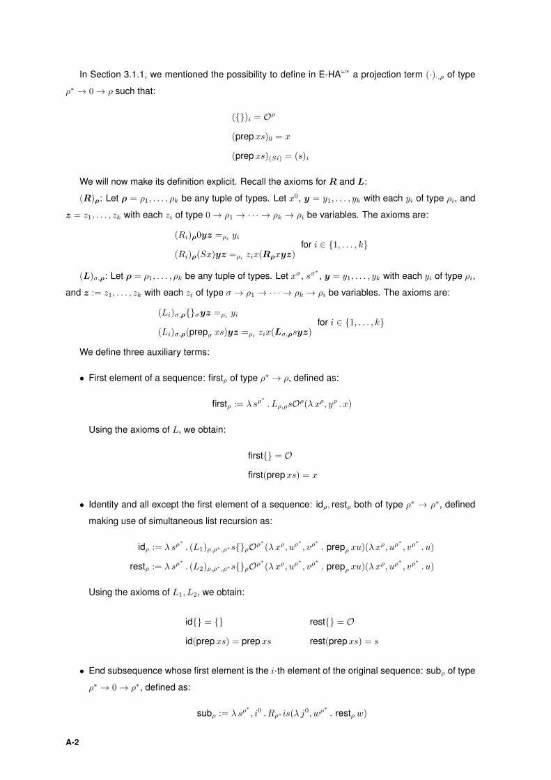
In Section 3.1.1, we mentioned the possibility to define in E-HAω∗ a projection term (·)·,ρ of type
ρ∗ → 0→ ρ such that:
({})i = Oρ
(prepxs)0 = x
(prepxs)(Si) = (s)i
We will now make its definition explicit. Recall the axioms for R and L:
(R)ρ: Let ρ = ρ1, . . . , ρk be any tuple of types. Let x0, y = y1, . . . , yk with each yi of type ρi, and
z = z1, . . . , zk with each zi of type 0→ ρ1 → · · · → ρk → ρi be variables. The axioms are:
(Ri)ρ0yz =ρi yi
(Ri)ρ(Sx)yz =ρi zix(Rρxyz)for i ∈ {1, . . . , k}
(L)σ,ρ: Let ρ = ρ1, . . . , ρk be any tuple of types. Let xσ, sσ∗, y = y1, . . . , yk with each yi of type ρi,
and z := z1, . . . , zk with each zi of type σ → ρ1 → · · · → ρk → ρi be variables. The axioms are:
(Li)σ,ρ{}σyz =ρi yi
(Li)σ,ρ(prepσ xs)yz =ρi zix(Lσ,ρsyz)for i ∈ {1, . . . , k}
We define three auxiliary terms:
• First element of a sequence: firstρ of type ρ∗ → ρ, defined as:
firstρ := λ sρ∗. Lρ,ρsOρ(λxρ, yρ . x)
Using the axioms of L, we obtain:
first{} = O
first(prepxs) = x
• Identity and all except the first element of a sequence: idρ, restρ both of type ρ∗ → ρ∗, defined
making use of simultaneous list recursion as:
idρ := λ sρ∗. (L1)ρ,ρ∗,ρ∗s{}ρOρ
∗(λxρ, uρ
∗, vρ
∗. prepρ xu)(λxρ, uρ
∗, vρ
∗. u)
restρ := λ sρ∗. (L2)ρ,ρ∗,ρ∗s{}ρOρ
∗(λxρ, uρ
∗, vρ
∗. prepρ xu)(λxρ, uρ
∗, vρ
∗. u)
Using the axioms of L1, L2, we obtain:
id{} = {} rest{} = O
id(prepxs) = prepxs rest(prepxs) = s
• End subsequence whose first element is the i-th element of the original sequence: subρ of type
ρ∗ → 0→ ρ∗, defined as:
subρ := λ sρ∗, i0 . Rρ∗is(λ j
0, wρ∗. restρ w)
A-2

Using the axioms of R and the above, we obtain:
sub s0 = s
sub s(Si) = rest(sub si)
For example, informally writing a list as {s0, s1, s2, s3, s4, s5}:
sub{s0, s1, s2, s3, s4, s5}(SSS0) = rest(rest(rest{s0, s1, s2, s3, s4, s5})) = {s3, s4, s5}
We are finally able to define the projection: (·)·,ρ of type ρ∗ → 0→ ρ as:
(·)·,ρ := λ sρ∗, i0 . Lρ,ρsOρ(λxρ, zρ . firstρ(subρ si))
We write (s)i instead of (·)·si. Using the axioms for L and the above, we obtain:
({})i = O
(prepxs)0 = first(sub(prepxs)0) = first(prepxs) = x
(prepxs)(Si) = first(sub(prepxs)(Si)) = (s)i
as desired.
A-3

A-4