on the implementation of gnu prolog -...
TRANSCRIPT
Under consideration for publication in Theory and Practice of Logic Programming 1
On the Implementation of GNU Prolog
DANIEL DIAZ
University of Paris 1
90 rue de Tolbiac75013 Paris, FRANCE
E-mail: [email protected]
SALVADOR ABREU
Universidade de Evora and CENTRIA FCT/UNL
Largo dos Colegiais 2
7004-516 Evora, PORTUGALE-mail: [email protected]
PHILIPPE CODOGNET
JFLI, CNRS / University of Tokyo
JAPANE-mail: [email protected]
submitted 4th October 2009; revised 1st March 2010; accepted 22nd November 2010
Abstract
GNU Prolog is a general-purpose implementation of the Prolog language, which distin-guishes itself from most other systems by being, above all else, a native-code compilerwhich produces standalone executables which don’t rely on any byte-code emulator ormeta-interpreter. Other aspects which stand out include the explicit organization of theProlog system as a multipass compiler, where intermediate representations are materi-alized, in Unix compiler tradition. GNU Prolog also includes an extensible and high-performance finite domain constraint solver, integrated with the Prolog language butimplemented using independent lower-level mechanisms. This article discusses the mainissues involved in designing and implementing GNU Prolog: requirements, system orga-nization, performance and portability issues as well as its position with respect to otherProlog system implementations and the ISO standardization initiative.
KEYWORDS: Prolog, logic programming system, GNU, ISO, WAM, native code compi-lation, Finite Domain constraints
1 Introduction
GNU Prolog’s roots go back to the start of the 1990s at the Logic Programming
research team at INRIA Rocquencourt, in Paris. Philippe Codognet planned on im-
plementing a low-level version of his intelligent backtracking techniques and opted
to do so on the state-of-the art SICStus Prolog system, for which he obtained the
source code. This task was handed down to Daniel Diaz, at that time an M.Sc. stu-
dent. However, at the time SICStus Prolog was already a very large scale and
2 D. Diaz, S. Abreu and P. Codognet
complex system: version 2.1 had about 70,000 lines of highly tuned and optimized
C and Prolog code: clearly not the easiest platform on which to carry out indepen-
dent, low-level experiments. So we took it upon ourselves to develop yet another
implementation of Prolog which would meet the following requirements:
• The system ought to serve as the basis for several research-oriented extensions
such as: intelligent backtracking, co-routining (freeze was a hot topic back
then), concurrency, constraints, etc.
• The system would be made available freely to all researchers.
• The system would be portable by design, not tied to any particular architecture.
• The core of the system must be simple and lightweight, unlike SICStus.
• The base system performance should be good. The rationale being that a system
designed to be extended needs to provide good base performance. We targeted
performance close to that of SICStus Prolog native code.
The last two points (simplicity and performance) were hard to reconcile. This was
particularly true at a time where research on WAM optimization was a hot topic:
choice points, backtracking, unification, indexing, register allocation, etc.: all as-
pects of the WAM were the object of published research on optimizations thereof.
The goals we had set for ourselves seemed difficult to reach and rather ambitious:
performance with a simple implementation, all done with little or no optimizations.
At the time, most Prolog systems were based on byte-code emulators, written in
C or assembly language. We decided we would need to compile to native code in
order to recoup the relative performance loss due to the inherent simplicity of the
WAM model we were to adopt. It remained to be seen how we would go about pro-
ducing native code. At the time, producing native code seemed to be the best thing
one could possibly do: see BIM-Prolog, SICStus Prolog, Aquarius Prolog, to name
a few. The SICStus approach was to retain its usual emulated byte-code and only
present the option of producing native code for select architectures1, which could be
transparently mixed with emulated predicates. The approach followed by Peter van
Roy with Aquarius Prolog was different and more traditional: compilation was sep-
arate from execution, as in regular programming languages (Van Roy and Despain
1992). A “command line” compiler would translate a Prolog program into a native-
code executable. Unfortunately, simplicity was apparently not a goal of the exercise:
Aquarius’ abstract machine, the BAM, was lower-level and finer-grained than the
WAM and comprised more than 100 instructions, some of which were specializa-
tions created on-the-fly by the compiler using abstract interpretation techniques.
Other “native code generation” approaches were surfacing, which would generate
C rather than an actual assembly language: these included Janus (Gudeman et al.
1992) which translated Prolog to C, KL/1 (Chikayama et al. 1994) which compiled
a language different from Prolog (a committed-choice language, with don’t-care
nondeterminism) or Erlang (Hausman 1993), a functional language only loosely re-
lated to Prolog. A significant difficulty that compilers to C had to deal with was the
1 Sparc under SunOS was the chosen one.
On the Implementation of GNU Prolog 3
orthogonal control dimension due to backtracking, which complicates stack frame
management beyond what C can normally do.
Our choice was to translate to C via the WAM, decorating the generated code
with direct assembly language instructions, to handle native jumps which cor-
respond to Prolog control transfers, such as the call, execute or proceed in-
structions. The system we built was called wamcc (Codognet and Diaz 1995) and
most WAM instructions were directly replaced by the equivalent C code, inlined at
compile-time via a set of C Preprocessor macros. More complex instructions result
in library function calls, this was the case with unification instructions, for exam-
ple. Lastly, wamcc was the first documented Prolog system to rely on the hardware
(MMU) to detect stack or heap overflows, by placing unmapped pages at the limits
of the dynamic memory areas: accessing these would raise an exception and inter-
rupt the normal flow of execution. This approach resulted in a clear performance
gain when compared with bounds checks being performed on every allocation and
was innovative at the time.2 Our choices clearly paid off, as wamcc got a 60% perfor-
mance gain w.r.t. emulated SICStus and about 30% performance loss w.r.t. SICStus
native, the agreed-upon references of the time.
Since then, wamcc has been used as a teaching tool in several universities and, out-
side INRIA, as the starting point for research work, e.g. (Ferreira and Damas 1999).
The next step ought to have been the implementation of intelligent backtracking in
wamcc. This was not to happen: our interest shifted to the blooming area of Con-
straint Logic Programming (Jaffar and Lassez 1987), which was suddenly and for
the first time enabling Logic Programming for large-scale industrial applications.
There is little doubt that Pascal Van Hentenryck’s PhD thesis work and the imple-
mentation of a Finite Domain (FD) solver in the CHIP language (Van Hentenryck
1989) were instrumental in CLP’s success. The CLP mechanisms underlying CHIP
were touted as highly optimized, totalling 50K lines of C code and shrouded in
wraps of secrecy – a very useful and interesting black box. It took a few years for
the work describing cc(FD) (Van Hentenryck et al. 1994) to provide hints as to
how an effective CLP system could be implemented. The following move for wamcc
was clear: it would become clp(FD) and introduce a simple extension to the WAM
to integrate FD constraints (Diaz and Codognet 1993; Codognet and Diaz 1996).
clp(FD) was about 4 times faster than CHIP.
The worst problem we had with wamcc (and consequently clp(FD)) was the exces-
sively long time it took GCC to compile the generated C code. Even for moderately-
sized programs, the time quickly became overwhelming and even our attempts to
banish most inlining in favour of library function calls were insufficient to bring the
times down to acceptable levels.
On closer inspection, the C language was being used as a machine-independent
assembly language, which we had to fool in order to do jumps. This went against the
regular operation of a C compiler, which expects regular function entry and exit to
be the norm: as a consequence the compiler was trying to do its task over programs
2 These days, this functionality is available off-the-shelf, in the form of the libsigsegv library,on http://libsigsegv.sourceforge.net/.
4 D. Diaz, S. Abreu and P. Codognet
which were really too devious and too large for it to properly cope. As we did not
really need all that C could express, we started looking for alternative languages
to compile into. One possibility which looked very interesting was C-- (Jones et al.
1997). Unfortunately this system was not developed to the point where it would be
actually useful for our purpose: it remains bound to a limited set of back-ends.3 We
then set out to specify and implement an intermediate language of our own. Our
“Mini-Assembly” (MA) language would have to meet very basic requirements: to
directly handle WAM control and be able to call C functions would be sufficient.
This simplicity was meant to promote the easy porting to common architectures.
At that time, the Prolog standardization effort was in full swing, which lead to the
emergence of the specification document known as ISO Core 1 (ISO-Part1 1995). We
then committed to develop a completely new, standard-compliant implementation
of Prolog, which would use the MA intermediate language instead of C in the
compiler pipeline. So was GNU Prolog born, under the code name Calypso.
The Prolog language was not very popular (euphemism alert!) outside the re-
search community, and in particular no implementation of the language was present
in the GNU organization catalogue, whereas other, similarly exotic languages such
as Scheme, were. We took it upon ourselves to defend our case with GNU in late
1998 and the first official release of GNU Prolog saw the light of day in April 1999.
GNU Prolog is presently directly available for most Linux distributions.
The remainder of this article is structured as follows: Section 2 discusses the
structure of the GNU Prolog compiler pipeline with fully fleshed-out examples. In
Section 3 we present GNU Prolog’s Constraint Logic Programming design and imple-
mentation. Section 4 tackles the positioning of GNU Prolog in the Prolog landscape
and its relation to the ISO standardization initiative. Finally, in Section 5 we draw
conclusions from the experience acquired over the last years and lay out possible
plans for further developments, some of which are actively being pursued by the
authors of the present article as well as other researchers.
2 Compilation Scheme
In this section we detail the compilation scheme adopted in GNU Prolog. As previ-
ously stated, the main design decision was to use a simple WAM and to compensate
for the lack of optimizations by producing native code, thereby avoiding the over-
head of an emulator. The compilation process is then the key point of GNU Prolog.
In wamcc, GNU Prolog’s ancestor, we produced native code via C: a Prolog file was
translated into a WAM file, itself translated to C and finally to object code, by the
C compiler. This approach had a major drawback: the time needed to compile the
C file; even for medium-sized Prolog sources, the time needed by the C compiler was
quickly dominating the entire compilation process. In GNU Prolog we decided to
sidestep the issue by not compiling to C but, instead, to directly generate assembly
code. The direct translation from the WAM to assembly code turns out to be a
3 For a long time C-- was restricted to 32-bit x86, and even though this situation has evolved,the set of target architectures is still smaller than what we have attained with the MA tool.
On the Implementation of GNU Prolog 5
significant effort as a translator must be written for each target architecture. We
simplified this problem by defining an intermediate language called Mini-Assembly
or MA for short, which can be viewed as a machine-independent assembly language
well suited to be the target of a WAM translator. This language will be detailed
below, in sections 2.2 and 2.3.
One of the design goals for GNU Prolog was to offer a system which can easily
be extended by other research teams. This requirement led us to split the compiler
into several passes, with distinct executables for which the respective intermediate
representations must be materialized as plain text files or streams. The passes are:
pl2wam which compiles a Prolog source file into WAM code.
wam2ma which converts the WAM code to the MA language.
ma2asm that translates the abstract MA code to architecture-specific machine instruc-
tions: its output is an assembly language program.
fd2c compiles FD constraint definitions into C functions which perform constraint
propagation at runtime. See section 3 for more on this.
In addition to those GNU Prolog-specific compiler components, the compilation
process also involves the standard tools:
as the assembler for the target architecture.
cc the C compiler
ld the link editor: to bind together all objects/libraries and provide a machine-
dependent executable.
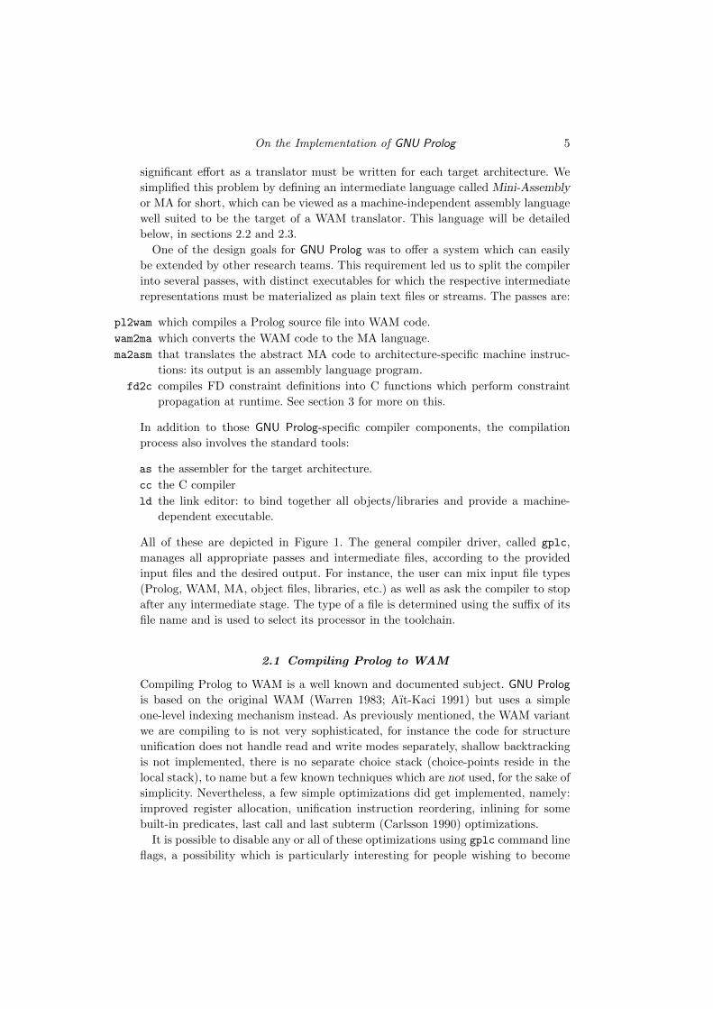
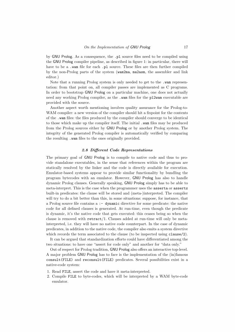
All of these are depicted in Figure 1. The general compiler driver, called gplc,
manages all appropriate passes and intermediate files, according to the provided
input files and the desired output. For instance, the user can mix input file types
(Prolog, WAM, MA, object files, libraries, etc.) as well as ask the compiler to stop
after any intermediate stage. The type of a file is determined using the suffix of its
file name and is used to select its processor in the toolchain.
2.1 Compiling Prolog to WAM
Compiling Prolog to WAM is a well known and documented subject. GNU Prolog
is based on the original WAM (Warren 1983; Aıt-Kaci 1991) but uses a simple
one-level indexing mechanism instead. As previously mentioned, the WAM variant
we are compiling to is not very sophisticated, for instance the code for structure
unification does not handle read and write modes separately, shallow backtracking
is not implemented, there is no separate choice stack (choice-points reside in the
local stack), to name but a few known techniques which are not used, for the sake of
simplicity. Nevertheless, a few simple optimizations did get implemented, namely:
improved register allocation, unification instruction reordering, inlining for some
built-in predicates, last call and last subterm (Carlsson 1990) optimizations.
It is possible to disable any or all of these optimizations using gplc command line
flags, a possibility which is particularly interesting for people wishing to become
6 D. Diaz, S. Abreu and P. Codognet
gplc
.pl
pl2wam
.wam
wam2ma
.ma
ma2asm
.s as
.fd
fd2c
.c
cc
.o files libraries
ld
executable
Fig. 1. Compilation Scheme
familiar with the WAM (e.g. students taking declarative programming language
implementation courses.)
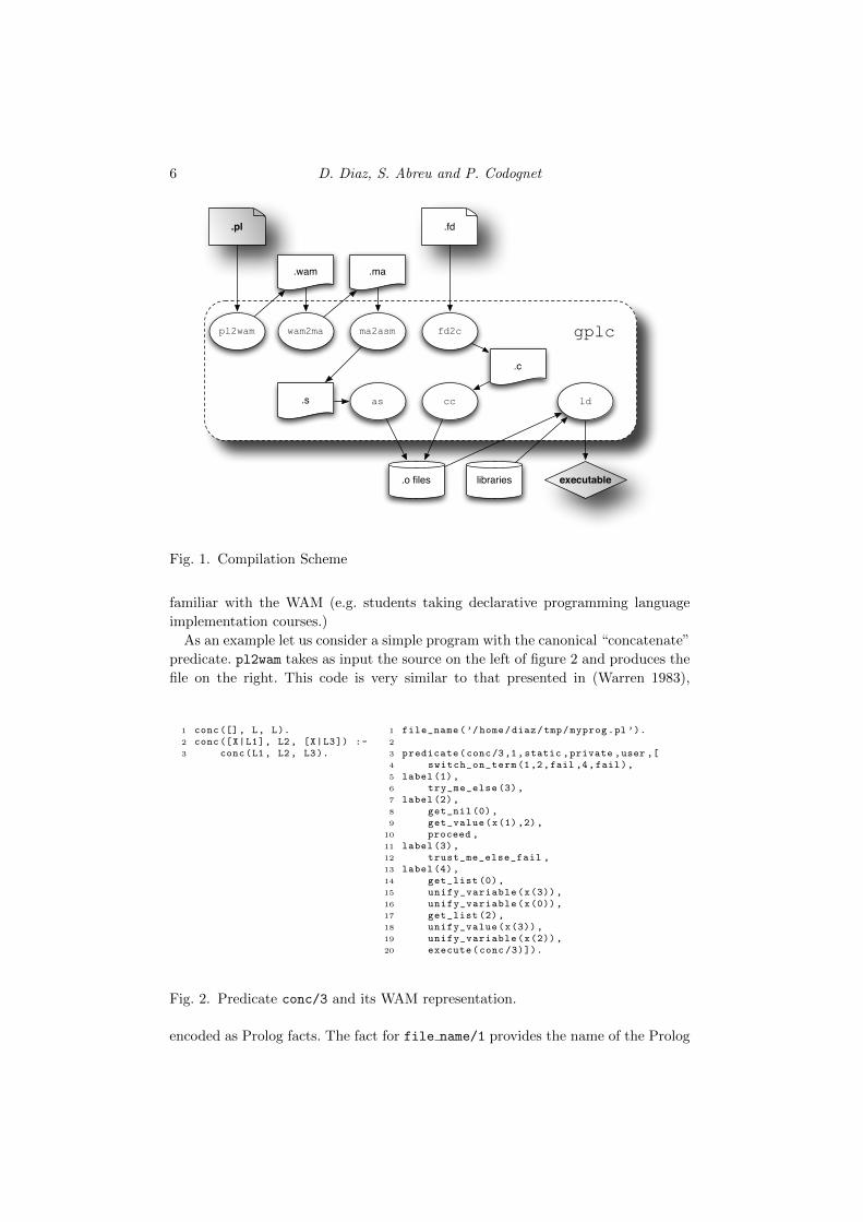
As an example let us consider a simple program with the canonical “concatenate”
predicate. pl2wam takes as input the source on the left of figure 2 and produces the
file on the right. This code is very similar to that presented in (Warren 1983),
1 conc([], L, L).2 conc([X|L1], L2 , [X|L3]) :-3 conc(L1 , L2 , L3).
1 file_name(’/home/diaz/tmp/myprog.pl ’).2
3 predicate(conc/3,1,static ,private ,user ,[4 switch_on_term (1,2,fail ,4,fail),5 label(1),6 try_me_else (3),7 label(2),8 get_nil (0),9 get_value(x(1),2),
10 proceed ,11 label(3),12 trust_me_else_fail ,13 label(4),14 get_list (0),15 unify_variable(x(3)),16 unify_variable(x(0)),17 get_list (2),18 unify_value(x(3)),19 unify_variable(x(2)),20 execute(conc /3)]).
Fig. 2. Predicate conc/3 and its WAM representation.
encoded as Prolog facts. The fact for file name/1 provides the name of the Prolog
On the Implementation of GNU Prolog 7
source file which applies to the subsequent predicate definitions. Note that several
instances of file name/1 may occur, as a result of include/1 directives. The fact
for predicate/6 contains the code for the predicate conc/3, as a list of WAM
instructions. Several predicate properties are also stated here: static (as opposed
to dynamic), private (as opposed to public) and user (as opposed to built-in).
This code can be easily read and understood by humans (useful for student use)
and it can also directly serve as input for a Prolog program like an emulator, a
source-to-source optimizer or another back-end as was done in the Prolog-to-EAM
compiler, reported on in (Andre and Abreu 2010). The drawbacks of this choice
are: a not very compact representation (see the length of the instruction names, for
instance) and the need for a non-trivial parser for the next stage which, in the case
of GNU Prolog, is handled by wam2ma.
As previously mentioned, the GNU Prolog WAM is not very optimized. Consider
the clause: p(a, X) :- q(a, X), r(X). Compiling it results in the following sub-
optimal code (2 WAM instructions could be avoided):
1 predicate(p/2,7,static ,private ,user ,[2 allocate (1),3 get_atom(a,0),4 get_variable(y(0),1),5 put_atom(a,0), % useless instruction !6 put_value(y(0),1), % useless instruction !7 call(q/2),8 put_value(y(0),0),9 deallocate ,
10 execute(r/1)]).
A WAM instruction cache could solve this as explained in (Carlsson 1990). Basically,
the cache remembers the current values of the WAM registers. When a put instruc-
tion occurs, if the cache detects the wanted data is already present in a register it
replaces the put instruction by a register move instruction (hoping the register opti-
mizer will delete this move intruction). Optimizations such as this are not included
in our current compiler, which remains simple–about 3000 lines of Prolog code–yet
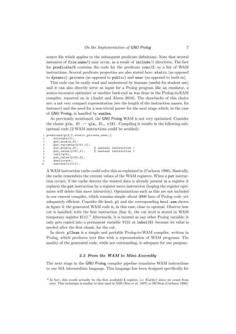
adequately efficient. Consider file bool.pl and the corresponding bool.wam shown
in figure 3: the generated WAM code is, in this case, close to optimal. Observe how
cut is handled: with the first instruction (line 4), the cut level is stored in WAM
temporary register X(1).4 Afterwards, it is treated as any other Prolog variable: it
only gets copied into a permanent variable–Y(0) at label(6)–because its value is
needed after the first chunk, for the cut.
In short: pl2wam is a simple and portable Prolog-to-WAM compiler, written in
Prolog, which produces text files with a representation of WAM programs. The
quality of the generated code, while not outstanding, is adequate for our purpose.
2.2 From the WAM to Mini-Assembly
The next stage in the GNU Prolog compiler pipeline translates WAM instructions
to our MA intermediate language. This language has been designed specifically for
4 In fact, this would actually be the first available X register, i.e. X(arity) since we count fromzero. This technique is similar to that used in XSB (Rao et al. 1997) or SICStus (Carlsson 1990).
8 D. Diaz, S. Abreu and P. Codognet
1 is_true(true).2
3 is_true(not(E)) :-4 is_true(E), !,5 fail.6 is_true(not(_)).7
8 is_true(and(E1, E2)) :-9 is_true(E1),
10 is_true(E2).
1 file_name(’/home/diaz/tmp/bool.pl ’).2
3 predicate(is_true /1,1,static ,private ,user ,[4 load_cut_level (1),5 switch_on_term (3,4,fail ,fail ,1),6 label(1),7 switch_on_structure ([( not/1,2),(and/2,10)]),8 label(2),9 try(6),
10 trust(8),11 label(3),12 try_me_else (5),13 label(4),14 get_atom(true ,0),15 proceed ,16 label(5),17 retry_me_else (7),18 label(6),19 allocate (1),20 get_structure(not/1,0),21 unify_variable(x(0)),22 get_variable(y(0),1),23 call(is_true /1),24 cut(y(0)),25 fail ,26 label(7),27 retry_me_else (9),28 label(8),29 get_structure(not/1,0),30 unify_void (1),31 proceed ,32 label(9),33 trust_me_else_fail ,34 label (10),35 allocate (1),36 get_structure(and/2,0),37 unify_variable(x(0)),38 unify_variable(y(0)),39 call(is_true /1),40 put_value(y(0),0),41 deallocate ,42 execute(is_true /1)]).
Fig. 3. Predicate is true/1 Prolog and WAM code.
the execution of Prolog based on our experience with wamcc when compiling down
to C: in wamcc most WAM instructions finally ended up as a C function call which
performed the associated task. Only a few instructions were inlined (via C macros)
because the size of the resulting code would have been prohibitive for the available
C compilers. In fact, C was being used as a sort of machine-independent assembler
but:
1. the C compiler was unaware of the situation and spent a lot of time analyzing
and optimizing the code and;
2. C is not truly an assembler and its control model is based on function definition
and calls, making the efficient handling of Prolog backtracking very difficult.
These problems drove us to design an intermediate representation, the Mini-Assembly
with the following features:
On the Implementation of GNU Prolog 9
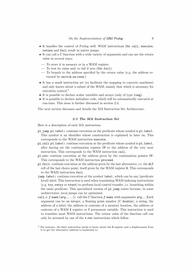
• It handles the control of Prolog well: WAM instructions like call, execute,
return and fail result in native jumps.
• It can call a C function with a wide variety of arguments and can use the return
value in several ways:
— To store it in memory or in a WAM register.
— To test its value and, to fail if zero (like fail).
— To branch to the address specified by the return value (e.g. the address re-
turned by switch on term.)
• It has a small instruction set (to facilitate the mapping to concrete machines)
and only knows about a subset of the WAM, mainly that which is necessary for
execution control.5
• It is possible to declare scalar variables and arrays (only of type long).
• It is possible to declare initializer code, which will be automatically executed at
run-time. This issue is further discussed in section 2.3.
The next section discusses and details the MA Instruction Set Architecture.
2.3 The MA Instruction Set
Here is a description of each MA instruction:
pl jump pl label : continue execution at the predicate whose symbol is pl label .
This symbol is an identifier whose construction is explained in later on. This
corresponds to the WAM instruction execute.
pl call pl label : continue execution at the predicate whose symbol is pl label ,
after having set the continuation register CP to the address of the very next
instruction. This corresponds to the WAM instruction call.
pl ret: continue execution at the address given by the continuation pointer CP.
This corresponds to the WAM instruction proceed.
pl fail: continue execution at the address given by the last alternative, i.e. the ALT
cell of the last choice point, itself given by the WAM register B. This corresponds
to the WAM instruction fail.
jump label : continue execution at the symbol label , which can be any (predicate
local) label. This instruction is used when translating WAM indexing instructions
(e.g. try, retry or trust) to perform local control transfer, i.e. branching within
the same predicate. This specialized version of pl jump exists because, in some
architectures, local jumps can be optimized.
call c f name (arg ,...): call the C function f name with arguments arg ,... Each
argument can be an integer, a floating point number (C double), a string, the
address of a label, the address or contents of a memory location, the address or
contents of a WAM X register or Y permanent variable. This instruction is used
to translate most WAM instructions. The return value of the function call can
only be accessed by one of the * ret instructions which follow.
5 For instance, the fail instruction needs to know about the B register and a displacement fromit to get the alternative address to backtrack to.
10 D. Diaz, S. Abreu and P. Codognet
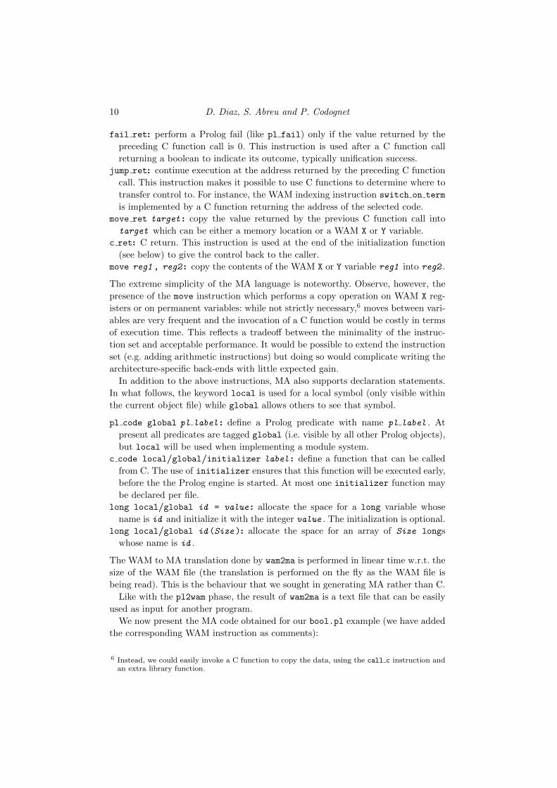
fail ret: perform a Prolog fail (like pl fail) only if the value returned by the
preceding C function call is 0. This instruction is used after a C function call
returning a boolean to indicate its outcome, typically unification success.
jump ret: continue execution at the address returned by the preceding C function
call. This instruction makes it possible to use C functions to determine where to
transfer control to. For instance, the WAM indexing instruction switch on term
is implemented by a C function returning the address of the selected code.
move ret target : copy the value returned by the previous C function call into
target which can be either a memory location or a WAM X or Y variable.
c ret: C return. This instruction is used at the end of the initialization function
(see below) to give the control back to the caller.
move reg1 , reg2 : copy the contents of the WAM X or Y variable reg1 into reg2 .
The extreme simplicity of the MA language is noteworthy. Observe, however, the
presence of the move instruction which performs a copy operation on WAM X reg-
isters or on permanent variables: while not strictly necessary,6 moves between vari-
ables are very frequent and the invocation of a C function would be costly in terms
of execution time. This reflects a tradeoff between the minimality of the instruc-
tion set and acceptable performance. It would be possible to extend the instruction
set (e.g. adding arithmetic instructions) but doing so would complicate writing the
architecture-specific back-ends with little expected gain.
In addition to the above instructions, MA also supports declaration statements.
In what follows, the keyword local is used for a local symbol (only visible within
the current object file) while global allows others to see that symbol.
pl code global pl label : define a Prolog predicate with name pl label . At
present all predicates are tagged global (i.e. visible by all other Prolog objects),
but local will be used when implementing a module system.
c code local/global/initializer label : define a function that can be called
from C. The use of initializer ensures that this function will be executed early,
before the the Prolog engine is started. At most one initializer function may
be declared per file.
long local/global id = value : allocate the space for a long variable whose
name is id and initialize it with the integer value . The initialization is optional.
long local/global id (Size ): allocate the space for an array of Size longs
whose name is id .
The WAM to MA translation done by wam2ma is performed in linear time w.r.t. the
size of the WAM file (the translation is performed on the fly as the WAM file is
being read). This is the behaviour that we sought in generating MA rather than C.
Like with the pl2wam phase, the result of wam2ma is a text file that can be easily
used as input for another program.
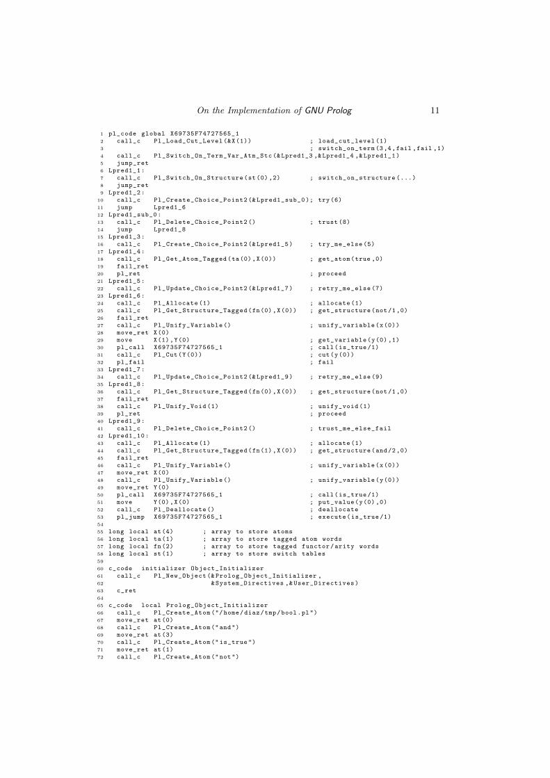
We now present the MA code obtained for our bool.pl example (we have added
the corresponding WAM instruction as comments):
6 Instead, we could easily invoke a C function to copy the data, using the call c instruction andan extra library function.
On the Implementation of GNU Prolog 11
1 pl_code global X69735F74727565_12 call_c Pl_Load_Cut_Level (&X(1)) ; load_cut_level (1)3 ; switch_on_term (3,4,fail ,fail ,1)4 call_c Pl_Switch_On_Term_Var_Atm_Stc (&Lpred1_3 ,&Lpred1_4 ,& Lpred1_1)5 jump_ret6 Lpred1_1:7 call_c Pl_Switch_On_Structure(st(0) ,2) ; switch_on_structure (...)8 jump_ret9 Lpred1_2:
10 call_c Pl_Create_Choice_Point2 (& Lpred1_sub_0 ); try(6)11 jump Lpred1_612 Lpred1_sub_0:13 call_c Pl_Delete_Choice_Point2 () ; trust (8)14 jump Lpred1_815 Lpred1_3:16 call_c Pl_Create_Choice_Point2 (& Lpred1_5) ; try_me_else (5)17 Lpred1_4:18 call_c Pl_Get_Atom_Tagged(ta(0),X(0)) ; get_atom(true ,0)19 fail_ret20 pl_ret ; proceed21 Lpred1_5:22 call_c Pl_Update_Choice_Point2 (& Lpred1_7) ; retry_me_else (7)23 Lpred1_6:24 call_c Pl_Allocate (1) ; allocate (1)25 call_c Pl_Get_Structure_Tagged(fn(0),X(0)) ; get_structure(not/1,0)26 fail_ret27 call_c Pl_Unify_Variable () ; unify_variable(x(0))28 move_ret X(0)29 move X(1),Y(0) ; get_variable(y(0) ,1)30 pl_call X69735F74727565_1 ; call(is_true /1)31 call_c Pl_Cut(Y(0)) ; cut(y(0))32 pl_fail ; fail33 Lpred1_7:34 call_c Pl_Update_Choice_Point2 (& Lpred1_9) ; retry_me_else (9)35 Lpred1_8:36 call_c Pl_Get_Structure_Tagged(fn(0),X(0)) ; get_structure(not/1,0)37 fail_ret38 call_c Pl_Unify_Void (1) ; unify_void (1)39 pl_ret ; proceed40 Lpred1_9:41 call_c Pl_Delete_Choice_Point2 () ; trust_me_else_fail42 Lpred1_10:43 call_c Pl_Allocate (1) ; allocate (1)44 call_c Pl_Get_Structure_Tagged(fn(1),X(0)) ; get_structure(and/2,0)45 fail_ret46 call_c Pl_Unify_Variable () ; unify_variable(x(0))47 move_ret X(0)48 call_c Pl_Unify_Variable () ; unify_variable(y(0))49 move_ret Y(0)50 pl_call X69735F74727565_1 ; call(is_true /1)51 move Y(0),X(0) ; put_value(y(0),0)52 call_c Pl_Deallocate () ; deallocate53 pl_jump X69735F74727565_1 ; execute(is_true /1)54
55 long local at(4) ; array to store atoms56 long local ta(1) ; array to store tagged atom words57 long local fn(2) ; array to store tagged functor/arity words58 long local st(1) ; array to store switch tables59
60 c_code initializer Object_Initializer61 call_c Pl_New_Object (& Prolog_Object_Initializer ,62 &System_Directives ,& User_Directives)63 c_ret64
65 c_code local Prolog_Object_Initializer66 call_c Pl_Create_Atom ("/ home/diaz/tmp/bool.pl")67 move_ret at(0)68 call_c Pl_Create_Atom ("and")69 move_ret at(3)70 call_c Pl_Create_Atom (" is_true ")71 move_ret at(1)72 call_c Pl_Create_Atom ("not")
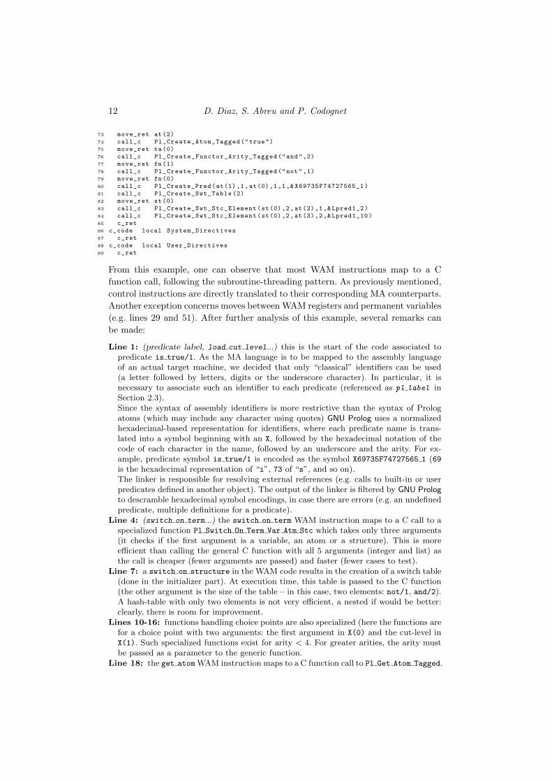
12 D. Diaz, S. Abreu and P. Codognet
73 move_ret at(2)74 call_c Pl_Create_Atom_Tagged ("true")75 move_ret ta(0)76 call_c Pl_Create_Functor_Arity_Tagged ("and",2)77 move_ret fn(1)78 call_c Pl_Create_Functor_Arity_Tagged ("not",1)79 move_ret fn(0)80 call_c Pl_Create_Pred(at(1),1,at(0),1,1,& X69735F74727565_1)81 call_c Pl_Create_Swt_Table (2)82 move_ret st(0)83 call_c Pl_Create_Swt_Stc_Element(st(0),2,at(2),1,& Lpred1_2)84 call_c Pl_Create_Swt_Stc_Element(st(0),2,at(3),2,& Lpred1_10)85 c_ret86 c_code local System_Directives87 c_ret88 c_code local User_Directives89 c_ret
From this example, one can observe that most WAM instructions map to a C
function call, following the subroutine-threading pattern. As previously mentioned,
control instructions are directly translated to their corresponding MA counterparts.
Another exception concerns moves between WAM registers and permanent variables
(e.g. lines 29 and 51). After further analysis of this example, several remarks can
be made:
Line 1: (predicate label, load cut level...) this is the start of the code associated topredicate is true/1. As the MA language is to be mapped to the assembly languageof an actual target machine, we decided that only “classical” identifiers can be used(a letter followed by letters, digits or the underscore character). In particular, it isnecessary to associate such an identifier to each predicate (referenced as pl label inSection 2.3).Since the syntax of assembly identifiers is more restrictive than the syntax of Prologatoms (which may include any character using quotes) GNU Prolog uses a normalizedhexadecimal-based representation for identifiers, where each predicate name is trans-lated into a symbol beginning with an X, followed by the hexadecimal notation of thecode of each character in the name, followed by an underscore and the arity. For ex-ample, predicate symbol is true/1 is encoded as the symbol X69735F74727565 1 (69is the hexadecimal representation of “i”, 73 of “s”, and so on).The linker is responsible for resolving external references (e.g. calls to built-in or userpredicates defined in another object). The output of the linker is filtered by GNU Prologto descramble hexadecimal symbol encodings, in case there are errors (e.g. an undefinedpredicate, multiple definitions for a predicate).
Line 4: (switch on term...) the switch on term WAM instruction maps to a C call to aspecialized function Pl Switch On Term Var Atm Stc which takes only three arguments(it checks if the first argument is a variable, an atom or a structure). This is moreefficient than calling the general C function with all 5 arguments (integer and list) asthe call is cheaper (fewer arguments are passed) and faster (fewer cases to test).
Line 7: a switch on structure in the WAM code results in the creation of a switch table(done in the initializer part). At execution time, this table is passed to the C function(the other argument is the size of the table – in this case, two elements: not/1, and/2).A hash-table with only two elements is not very efficient, a nested if would be better:clearly, there is room for improvement.
Lines 10-16: functions handling choice points are also specialized (here the functions arefor a choice point with two arguments: the first argument in X(0) and the cut-level inX(1). Such specialized functions exist for arity < 4. For greater arities, the arity mustbe passed as a parameter to the generic function.
Line 18: the get atom WAM instruction maps to a C function call to Pl Get Atom Tagged.
On the Implementation of GNU Prolog 13
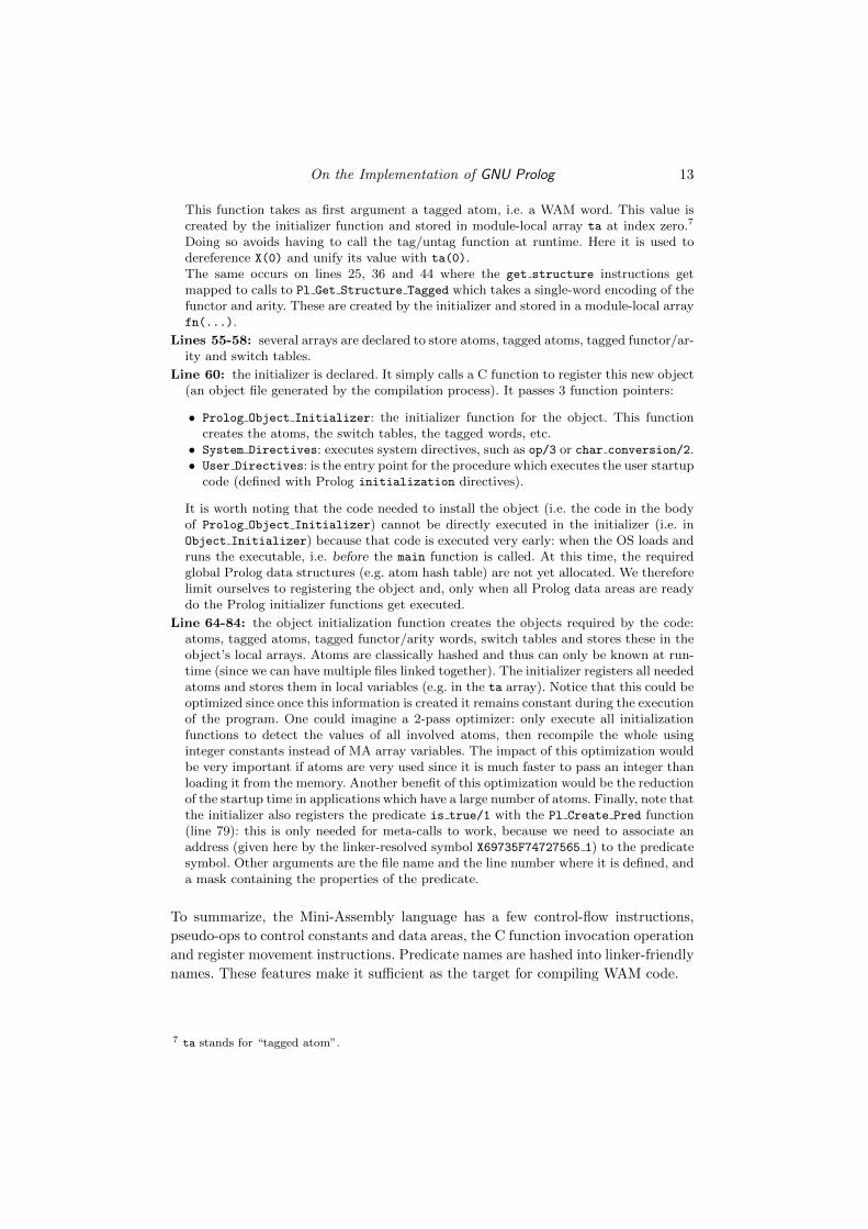
This function takes as first argument a tagged atom, i.e. a WAM word. This value iscreated by the initializer function and stored in module-local array ta at index zero.7
Doing so avoids having to call the tag/untag function at runtime. Here it is used todereference X(0) and unify its value with ta(0).The same occurs on lines 25, 36 and 44 where the get structure instructions getmapped to calls to Pl Get Structure Tagged which takes a single-word encoding of thefunctor and arity. These are created by the initializer and stored in a module-local arrayfn(...).
Lines 55-58: several arrays are declared to store atoms, tagged atoms, tagged functor/ar-ity and switch tables.
Line 60: the initializer is declared. It simply calls a C function to register this new object(an object file generated by the compilation process). It passes 3 function pointers:
• Prolog Object Initializer: the initializer function for the object. This functioncreates the atoms, the switch tables, the tagged words, etc.
• System Directives: executes system directives, such as op/3 or char conversion/2.• User Directives: is the entry point for the procedure which executes the user startup
code (defined with Prolog initialization directives).
It is worth noting that the code needed to install the object (i.e. the code in the bodyof Prolog Object Initializer) cannot be directly executed in the initializer (i.e. inObject Initializer) because that code is executed very early: when the OS loads andruns the executable, i.e. before the main function is called. At this time, the requiredglobal Prolog data structures (e.g. atom hash table) are not yet allocated. We thereforelimit ourselves to registering the object and, only when all Prolog data areas are readydo the Prolog initializer functions get executed.
Line 64-84: the object initialization function creates the objects required by the code:atoms, tagged atoms, tagged functor/arity words, switch tables and stores these in theobject’s local arrays. Atoms are classically hashed and thus can only be known at run-time (since we can have multiple files linked together). The initializer registers all neededatoms and stores them in local variables (e.g. in the ta array). Notice that this could beoptimized since once this information is created it remains constant during the executionof the program. One could imagine a 2-pass optimizer: only execute all initializationfunctions to detect the values of all involved atoms, then recompile the whole usinginteger constants instead of MA array variables. The impact of this optimization wouldbe very important if atoms are very used since it is much faster to pass an integer thanloading it from the memory. Another benefit of this optimization would be the reductionof the startup time in applications which have a large number of atoms. Finally, note thatthe initializer also registers the predicate is true/1 with the Pl Create Pred function(line 79): this is only needed for meta-calls to work, because we need to associate anaddress (given here by the linker-resolved symbol X69735F74727565 1) to the predicatesymbol. Other arguments are the file name and the line number where it is defined, anda mask containing the properties of the predicate.
To summarize, the Mini-Assembly language has a few control-flow instructions,
pseudo-ops to control constants and data areas, the C function invocation operation
and register movement instructions. Predicate names are hashed into linker-friendly
names. These features make it sufficient as the target for compiling WAM code.
7 ta stands for “tagged atom”.
14 D. Diaz, S. Abreu and P. Codognet
2.4 From Mini-Assembly to Actual Assembly
The next stage consists of mapping the MA language generated in the previous
section to the target machine’s actual instructions. Since MA is based on a very
small instruction set, the writing of such a translator is inherently simple. However,
producing machine instructions is not an easy task. The first MA-to-assembly lan-
guage mapper was written with the help of snippets taken from a C file produced
by wamcc: indeed, compiling a Prolog file to assembly by means of gcc gave us a
starting point for the translation, as the MA instructions correspond to a subset of
the C code. We then generalized this approach by defining a C file, each portion of
which corresponds to an MA instruction: the study of the assembly code produced
by gcc was our reference. This provided preliminary information about register use
conventions, C calling conventions, etc. However, in order to complete the assembly
code generator, we need to refer to the technical documentation of the processor
together with the ABI (Application Binary Interface) used by the operating system.
We now show portions of the assembly code for the previous example, using
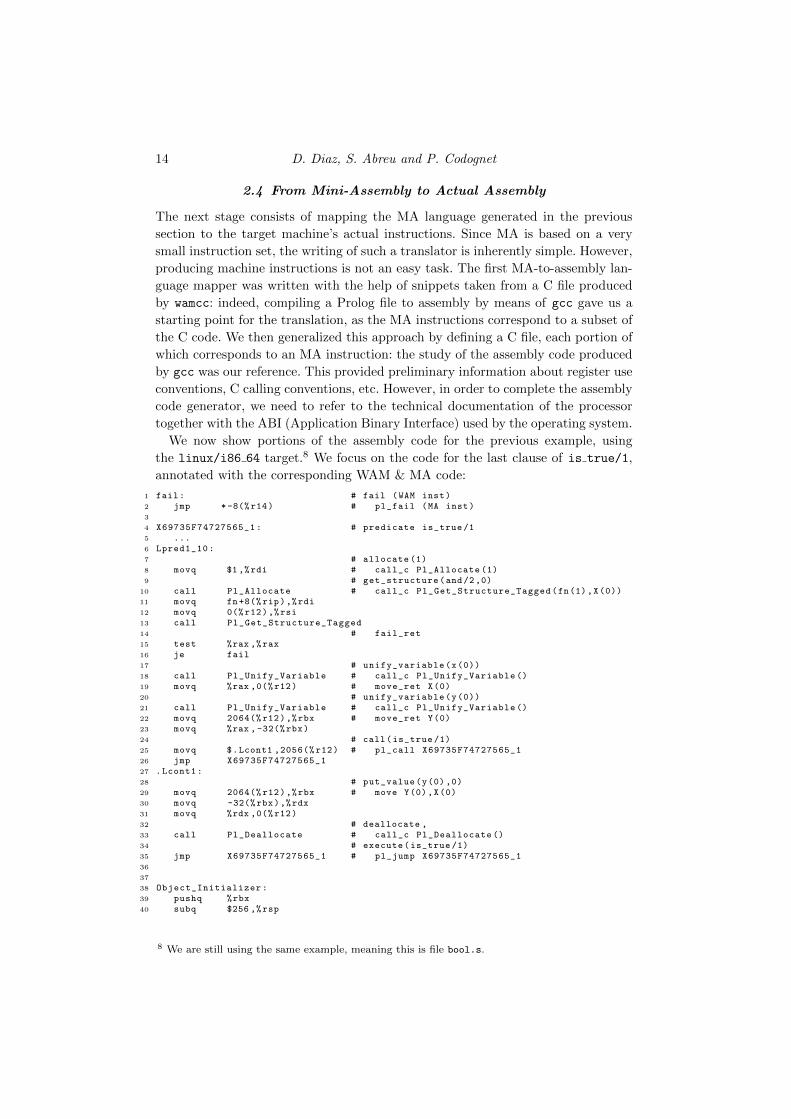
the linux/i86 64 target.8 We focus on the code for the last clause of is true/1,
annotated with the corresponding WAM & MA code:
1 fail: # fail (WAM inst)2 jmp *-8(%r14) # pl_fail (MA inst)3
4 X69735F74727565_1: # predicate is_true /15 ...6 Lpred1_10:7 # allocate (1)8 movq $1 ,%rdi # call_c Pl_Allocate (1)9 # get_structure(and/2,0)
10 call Pl_Allocate # call_c Pl_Get_Structure_Tagged(fn(1),X(0))11 movq fn+8(% rip),%rdi12 movq 0(%r12),%rsi13 call Pl_Get_Structure_Tagged14 # fail_ret15 test %rax ,%rax16 je fail17 # unify_variable(x(0))18 call Pl_Unify_Variable # call_c Pl_Unify_Variable ()19 movq %rax ,0(% r12) # move_ret X(0)20 # unify_variable(y(0))21 call Pl_Unify_Variable # call_c Pl_Unify_Variable ()22 movq 2064(% r12),%rbx # move_ret Y(0)23 movq %rax ,-32(%rbx)24 # call(is_true /1)25 movq $.Lcont1 ,2056(% r12) # pl_call X69735F74727565_126 jmp X69735F74727565_127 .Lcont1:28 # put_value(y(0),0)29 movq 2064(% r12),%rbx # move Y(0),X(0)30 movq -32(%rbx),%rdx31 movq %rdx ,0(% r12)32 # deallocate ,33 call Pl_Deallocate # call_c Pl_Deallocate ()34 # execute(is_true /1)35 jmp X69735F74727565_1 # pl_jump X69735F74727565_136
37
38 Object_Initializer:39 pushq %rbx40 subq $256 ,%rsp
8 We are still using the same example, meaning this is file bool.s.
On the Implementation of GNU Prolog 15
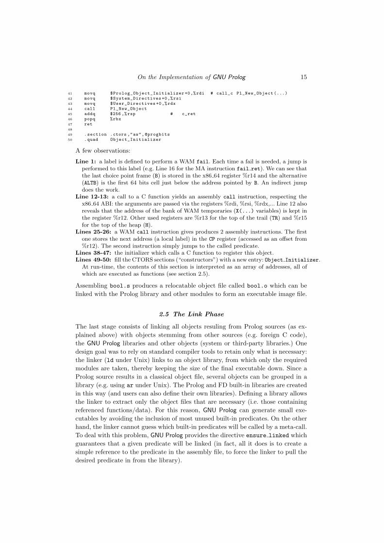
41 movq $Prolog_Object_Initializer +0,%rdi # call_c Pl_New_Object (...)42 movq $System_Directives +0,%rsi43 movq $User_Directives +0,%rdx44 call Pl_New_Object45 addq $256 ,%rsp # c_ret46 popq %rbx47 ret48
49 .section .ctors ,"aw",@progbits50 .quad Object_Initializer
A few observations:
Line 1: a label is defined to perform a WAM fail. Each time a fail is needed, a jump isperformed to this label (e.g. Line 16 for the MA instruction fail ret). We can see thatthe last choice point frame (B) is stored in the x86 64 register %r14 and the alternative(ALTB) is the first 64 bits cell just below the address pointed by B. An indirect jumpdoes the work.
Line 12-13: a call to a C function yields an assembly call instruction, respecting thex86 64 ABI: the arguments are passed via the registers %rdi, %rsi, %rdx,... Line 12 alsoreveals that the address of the bank of WAM temporaries (X(...) variables) is kept inthe register %r12. Other used registers are %r13 for the top of the trail (TR) and %r15for the top of the heap (H).
Lines 25-26: a WAM call instruction gives produces 2 assembly instructions. The firstone stores the next address (a local label) in the CP register (accessed as an offset from%r12). The second instruction simply jumps to the called predicate.
Lines 38-47: the initializer which calls a C function to register this object.Lines 49-50: fill the CTORS sections (“constructors”) with a new entry: Object Initializer.
At run-time, the contents of this section is interpreted as an array of addresses, all ofwhich are executed as functions (see section 2.5).
Assembling bool.s produces a relocatable object file called bool.o which can be
linked with the Prolog library and other modules to form an executable image file.
2.5 The Link Phase
The last stage consists of linking all objects resuling from Prolog sources (as ex-
plained above) with objects stemming from other sources (e.g. foreign C code),
the GNU Prolog libraries and other objects (system or third-party libraries.) One
design goal was to rely on standard compiler tools to retain only what is necessary:
the linker (ld under Unix) links to an object library, from which only the required
modules are taken, thereby keeping the size of the final executable down. Since a
Prolog source results in a classical object file, several objects can be grouped in a
library (e.g. using ar under Unix). The Prolog and FD built-in libraries are created
in this way (and users can also define their own libraries). Defining a library allows
the linker to extract only the object files that are necessary (i.e. those containing
referenced functions/data). For this reason, GNU Prolog can generate small exe-
cutables by avoiding the inclusion of most unused built-in predicates. On the other
hand, the linker cannot guess which built-in predicates will be called by a meta-call.
To deal with this problem, GNU Prolog provides the directive ensure linked which
guarantees that a given predicate will be linked (in fact, all it does is to create a
simple reference to the predicate in the assembly file, to force the linker to pull the
desired predicate in from the library).
16 D. Diaz, S. Abreu and P. Codognet
As previously stated, each linked object includes initialization code in which
various housekeeping functions are performed. This function gets executed before
any compiled Prolog code. The ELF format allows the specification of global Object-
Oriented constructor code, which gets executed at the start and is collected from
several object modules. We use this mechanism to initialize GNU Prolog objects.
2.6 GNU Prolog Executable Behaviour
From the user point of view, the behaviour of an executable produced by GNU Prolog
consists of executing all intialization/1 directives. If several initialization/1
directives appear in the same file they are executed in the order of appearance. If
several initialization/1 directives appear in different Prolog files (i.e. in different
objects) the order in which they are executed is implementation-defined. However,
on most machines the order will turn out to be the reverse of the order in which
the associated files have been linked. The traditional Prolog interactive top-level
interpreter is optionally linked with the rest of the executable. Should it be present,
it gets executed after all the other initialization/1 directives have finished. This
default behaviour is provided as a main function defined in the GNU Prolog library.
So in the absence of a user-defined main function the default function is executed.
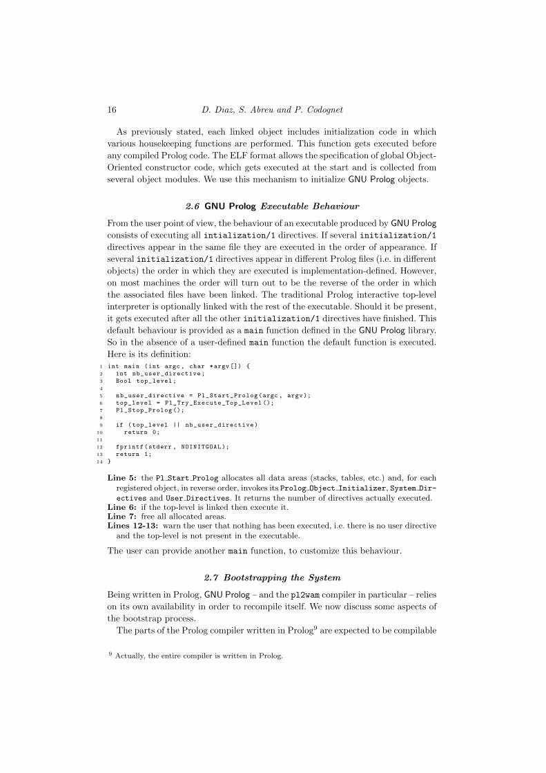
Here is its definition:1 int main (int argc , char *argv []) {2 int nb_user_directive;3 Bool top_level;4
5 nb_user_directive = Pl_Start_Prolog(argc , argv);6 top_level = Pl_Try_Execute_Top_Level ();7 Pl_Stop_Prolog ();8
9 if (top_level || nb_user_directive)10 return 0;11
12 fprintf(stderr , NOINITGOAL );13 return 1;14 }
Line 5: the Pl Start Prolog allocates all data areas (stacks, tables, etc.) and, for eachregistered object, in reverse order, invokes its Prolog Object Initializer, System Dir-
ectives and User Directives. It returns the number of directives actually executed.Line 6: if the top-level is linked then execute it.Line 7: free all allocated areas.Lines 12-13: warn the user that nothing has been executed, i.e. there is no user directive
and the top-level is not present in the executable.
The user can provide another main function, to customize this behaviour.
2.7 Bootstrapping the System
Being written in Prolog, GNU Prolog – and the pl2wam compiler in particular – relies
on its own availability in order to recompile itself. We now discuss some aspects of
the bootstrap process.
The parts of the Prolog compiler written in Prolog9 are expected to be compilable
9 Actually, the entire compiler is written in Prolog.
On the Implementation of GNU Prolog 17
by GNU Prolog. As a consequence, the .pl source files need to be compiled using
the GNU Prolog compiler pipeline, as described in figure 1: in particular, there will
have to be a .wam file for each .pl source. These files are then further compiled
by the non-Prolog parts of the system (wam2ma, ma2asm, the assembler and link
editor.)
Note that a running Prolog system is only needed to get to the .wam represen-
tation: from that point on, all compiler passes are implemented as C programs.
In order to bootstrap GNU Prolog on a particular machine, one does not actually
need any working Prolog compiler, as the .wam files for the pl2wam executable are
provided with the source.
Another aspect worth mentioning involves quality assurance for the Prolog-to-
WAM compiler: a new version of the compiler should hit a fixpoint for the contents
of the .wam files: the files produced by the compiler should converge to be identical
to those which make up the compiler itself. The initial .wam files may be produced
from the Prolog sources either by GNU Prolog or by another Prolog system. The
integrity of the generated Prolog compiler is automatically verified by comparing
the resulting .wam files to the ones originally provided.
2.8 Different Code Representations
The primary goal of GNU Prolog is to compile to native code and thus to pro-
vide standalone executables, in the sense that references within the program are
statically resolved by the linker and the code is directly available for execution.
Emulator-based systems appear to provide similar functionality by bundling the
program bytecodes with an emulator. However, GNU Prolog has also to handle
dynamic Prolog clauses. Generally speaking, GNU Prolog simply has to be able to
meta-interpret. This is the case when the programmer uses the asserta or assertz
built-in predicates: the clause will be stored and (meta-)interpreted. The compiler
will try to do a bit better than this, in some situations: suppose, for instance, that
a Prolog source file contains a :- dynamic directive for some predicate: the native
code for all defined clauses is generated. At run-time, even though the predicate
is dynamic, it’s the native code that gets executed: this ceases being so when the
clause is removed with retract/1. Clauses added at run-time will only be meta-
interpreted, i.e. they will have no native code counterpart. In the case of dynamic
predicates, in addition to the native code, the compiler also emits a system directive
which records the term associated to the clause (to be inspected using clause/2).
It can be argued that standardization efforts could have differentiated among the
two situations: to have one “assert for code only” and another for “data only.”
Out of respect for Prolog tradition, GNU Prolog also offers an interactive top-level.
A major problem GNU Prolog has to face is the implementation of the (in)famous
consult(FILE) and reconsult(FILE) predicates. Several possibilities exist in a
native-code system:
1. Read FILE, assert the code and have it meta-interpreted.2. Compile FILE to byte-codes, which will be interpreted by a WAM byte-code
emulator.
18 D. Diaz, S. Abreu and P. Codognet
3. Compile FILE to native code and find a solution to dynamically load it into the
running process.
The first solution is simple to implement but obviously not very efficient. For the
time being, we settled for the second solution: we have developed a simple emulator
to execute a binary representation of the code provided by pl2wam. This emulator
is not optimized at all but provides a speedup of about 3 when compared to meta-
interpreted code.
We plan on moving to the third approach, which is becoming feasible in a portable
way by resorting to native shared libraries, which can be dynamically loaded or
released from the running process memory. Following this route frees us from having
to use the byte-code interpreter. On the downside, the production of native code
that can be dynamically loaded is a bit more demanding because the machine code
has to be position-independent, which requires rewriting of the architecture-specific
back-ends for ma2asm.
To summarize, GNU Prolog currently manages three kinds of code:
• interpreted code for meta-call and dynamically asserted clauses
• emulated (byte-)code for consulted predicates
• native code for statically compiled predicates
As a result, these three ways of representing and executing Prolog programs need
to be integrated, which turned out to be a demanding requirement, as these models
differ quite a bit. GNU Prolog has by no means the exclusivity as far as this aspect
is concerned: other Prolog systems need to represent programs in more than two
ways (BIM-Prolog and SICStus for instance.)
2.9 Discussion
This concludes the presentation of the GNU Prolog compilation scheme. Some goals
or aspects of the system are comparable to other systems, for instance the native
code implementation for SICStus Prolog of (Haygood 1994) or Aquarius (Van Roy
and Despain 1992) which also aim at compiling Prolog to interpreter-less native
code for real architectures.
With respect to the direct generation of native code as opposed to going through
C, the latter has the advantage that it is easier to set up, more portable and
maintainable. The downsides include high compilation times (as a result of using
a general-purpose, optimizing C compiler), relatively low performance when gen-
erating standard C code and, should one strive to improve performance by using
nonstandard extensions to the C language, the maintenance effort of the C compiler
itself. Our option of direct native code generation benefits from much better compi-
lation times and potentially very high performance at runtime. The main drawback
of this approach is its maintainability: new targets must be explicitly programmed
and adding new cross-cutting features to the language or model requires an adap-
tation of all the back-ends (e.g. threads or dynamic linking.)
Native code generation is usually aimed at high performance. The potential is
On the Implementation of GNU Prolog 19
high: absolute control over hardware register usage,10 optimal tagging schemes,
precise control flow, to name but a few aspects. However, in order to tap into this
potential, rich intermediate representations need to be devised. Such was the op-
tion in Aquarius Prolog, which defined the BAM (Van Roy and Despain 1992),
significantly different from the WAM, including several “realistic” low-level fine-
granularity instructions. Likewise, native code generation within SICStus Prolog
led to the definition of an intermediate language, the SAM (SICStus Abstract Ma-
chine) which was translated into M68K assembler or, alternatively, further compiled
into yet another low level representation (RISS) which was then mapped to a spe-
cific machine language (Sparc or MIPS). Neither survived: the Aquarius compiler
remained unusably slow and native code generation was dropped from SICStus
because of its maintenance requirements.
It can be argued that most efforts in designing and implementing lower-level
abstract machines for Prolog were targeting RISC architectures. For instance it
used to be a challenge to effectively use the fine-grained control of pipeline and
instruction flow that was typical of, say, MIPS or Sparc processors. Nowadays,
most available microprocessors implement a common architecture (x86 or x86-64)
but specific hardware implementations have sufficiently differing pipeline structures
that it becomes very difficult to optimize for any one of these. Besides, dynamic
instruction reordering also makes static instruction scheduling a largely moot point.
Performance in modern architectures is heavily dependent on making good use
of the memory cache hierarchies; Prolog compiler writers stand to gain a lot from
making good use of cache organizations, possibly more so than what can be bought
by other optimization techniques. The problem is that there is a lot of variation
across systems that must be accounted for to extract optimal performance.
It turns out that the more sophisticated approaches to native code generation
for Prolog have somehow vanished in the long run, while GNU Prolog remains up-
to-date and has been ported to several low-level architectures. We feel we have
achieved a good balance between simplicity, maintainability and performance. To
pursue performance gains without sacrificing simplicity we are investigating a re-
placement for the MA level in GNU Prolog: we are presently evaluating tools such
as LLVM (Lattner and Adve 2004) which can be thought of as a typed, machine-
independent assembly language.
3 Finite-Domain Constraints
The main extension built on top of wamcc was arguably clp(FD), which added con-
straint solving over Finite Domains (FD). GNU Prolog compiles FD constraints in a
way similar to its predecessor clp(FD), the approach being described in (Codognet
and Diaz 1996; Diaz and Codognet 1993). It is based on a so-called “RISC ap-
proach” which consists of translating, at compile-time, all complex user-constraints
(e.g. disequations, linear equations or inequations) into simple, primitive constraints
10 Being able to use hardware registers favours a register-based abstract machine such as theWAM, as opposed to other approaches.
20 D. Diaz, S. Abreu and P. Codognet
(the FD constraint system) which operate at a lower level and which really embody
the propagation mechanism for constraint solving. We shall first present the basic
ideas of the FD constraint system and then detail the extensions to this framework
implemented in GNU Prolog.
The FD Constraint System was originally proposed by Pascal Van Hentenryck
in the concurrent constraint setting (Van Hentenryck et al. 1994), and an efficient
implementation in the clp(FD) system is described in (Codognet and Diaz 1996;
Diaz and Codognet 1993). FD is based on a single primitive constraint with which
complex constraints are encoded: for example, constraints such as X = Y or X ≤2Y are defined by means of FD constraints, instead of having to be explicitly built
into the theory. Each constraint is made of a set of propagation rules describing
how the domain of each variable is related to the domain of the other variables, i.e.
rules for describing node and arc consistency propagation (see for instance (Tsang
1993) for more details on CSPs and consistency algorithms.)
A constraint is a formula of the form X in r where X is a variable and r is
a range. A range in FD is a non empty finite set of natural numbers. Intuitively,
a constraint X in r enforces that X belongs to the range denoted by r . Such a
range can be a constant range (e.g. 1..10) or an indexical range, when it contains
one or more of the following:
• dom(Y ) which represents the whole current domain of Y ;
• min(Y ) which represents the minimal value of the current domain of Y ;
• max(Y ) which represents the maximal value of the current domain of Y .
• val(Y ) which represents the final value Y (i.e. the domain of Y has been
reduced to a singleton). A constraint involving such an indexical is delayed
until Y is determined.
Obviously, when Y is instantiated, all indexicals evaluate to its value. When an
X in r constraint uses an indexical term depending on another variable Y it
becomes store-sensitive and must be checked each time the domain of Y is updated.
This is how consistency checking and domain reduction is achieved.
Complex constraints such as linear equations or inequations, as well as symbolic
constraints can be defined in terms of FD constraints, see (Codognet and Diaz 1996)
for more details. For instance, the constraint X ≤ Y , is translated as follows:11
X≤Y ≡ X in 0..max(Y) ∧ Y in min(X)..∞
Notice that this translation also has an operational flavor and specifies, for a given
n-ary constraint, how the domain of a variable may be updated in terms of the other
variables. For example, consider the FD constraint X in 0..max(Y): whenever the
largest value of the domain of Y changes (i.e. decreases), the domain of X must
be reduced. If, on the other hand, the domain of Y changes but its largest value
remains the same, then the domain of X does not change. One can therefore consider
those primitive X in r constraints as a low-level language in which to express the
propagation scheme. Indeed, it is possible to express in the constraint definition
11 In this discussion, we’re not using the GNU Prolog concrete syntax for constraint goals.
On the Implementation of GNU Prolog 21
(i.e. the translation of a high-level user constraint into a set of primitive constraints)
the propagation scheme chosen to solve the constraint: forward-checking, full or
partial look-ahead, according to the use of dom or min/max indexical terms.
3.1 The Constraint Definition Language
For GNU Prolog, we designed a specific language to define FD constraints which is
both flexible and powerful. The basic X in r is sufficient to define simple arith-
metic constraints but too restrictive to handle constraints like min(X ,Y ) = Z or
reified constraints, both of which need some form of delay mechanism. Another
limitation is that it is not possible to explicitly indicate the triggers for a particular
propagator: these are deduced from the indexical used in the X in r primitives.
The GNU Prolog constraint definition language, FD, has then been designed to allow
the user to define complex constraints and proposes various constructs to overcome
these limitations. FD programs are compiled into C by the fd2c translator. The re-
sulting C program is then compiled and the object fits into the compilation scheme
shown in Figure 1. We present the main features of the constraint definition lan-
guage by means of a few examples.
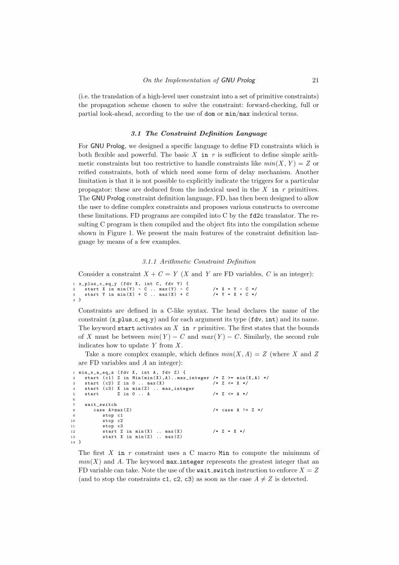
3.1.1 Arithmetic Constraint Definition
Consider a constraint X + C = Y (X and Y are FD variables, C is an integer):
1 x_plus_c_eq_y (fdv X, int C, fdv Y) {2 start X in min(Y) - C .. max(Y) - C /* X = Y - C */3 start Y in min(X) + C .. max(X) + C /* Y = X + C */4 }
Constraints are defined in a C-like syntax. The head declares the name of the
constraint (x plus c eq y) and for each argument its type (fdv, int) and its name.
The keyword start activates an X in r primitive. The first states that the bounds
of X must be between min(Y ) − C and max (Y ) − C . Similarly, the second rule
indicates how to update Y from X .
Take a more complex example, which defines min(X ,A) = Z (where X and Z
are FD variables and A an integer):
1 min_x_a_eq_z (fdv X, int A, fdv Z) {2 start (c1) Z in Min(min(X),A).. max_integer /* Z >= min(X,A) */3 start (c2) Z in 0 .. max(X) /* Z <= X */4 start (c3) X in min(Z) .. max_integer5 start Z in 0 .. A /* Z <= A */6
7 wait_switch8 case A>max(Z) /* case A != Z */9 stop c1
10 stop c211 stop c312 start Z in min(X) .. max(X) /* Z = X */13 start X in min(Z) .. max(Z)14 }
The first X in r constraint uses a C macro Min to compute the minimum of
min(X ) and A. The keyword max integer represents the greatest integer that an
FD variable can take. Note the use of the wait switch instruction to enforce X = Z
(and to stop the constraints c1, c2, c3) as soon as the case A 6= Z is detected.
22 D. Diaz, S. Abreu and P. Codognet
3.1.2 Reified Constraint Definition
The facility offered by the language to delay the activation of an X in r constraint
makes it possible to define reified constraints: the basic idea of a reified constraint is
to consider the truth value of a constraint as a first-class object, which is given the
form (“reified”) of a boolean value. This allows the user to make assumptions about
the satisfiability of constraints in a given store in order to conditionally require that
other constraints be met. It is feasible to use this mechanism, for instance, to define
disjunctive constraints, which can be very useful to model complex problems.
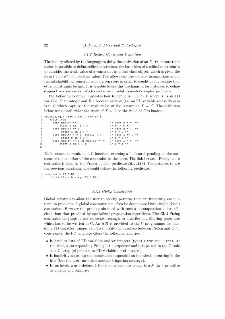
The following example illustrates how to define X = C ⇔ B where X is an FD
variable, C an integer and B a boolean variable (i.e. an FD variable whose domain
is 0..1) which captures the truth value of the constraint X = C . The definition
below waits until either the truth of X = C or the value of B is known:
1 truth_x_eq_c (fdv X,int C,fdv B) {2 wait_switch3 case max(B) == 0 /* case B = 0 */4 start X in ~{ C } /* X != C */5 case min(B) == 1 /* case B = 1 */6 start X in { C } /* X = C */7 case min(X) > C || max(X) < C /* case X != C */8 start B in { 0 } /* B = 0 */9 case min(X) == C && max(X) == C /* case X = C */
10 start B in { 1 } /* B = 1 */11 }
Each constraint results in a C function returning a boolean depending on the out-
come of the addition of the constraint to the store. The link between Prolog and a
constraint is done by the Prolog built-in predicate fd tell/1. For instance, to use
the previous constraint one could define the following predicate:
1 ’x=c <=> b’(X,C,B) :-2 fd_tell(truth_x_eq_c(X,C,B)).
3.1.3 Global Constraints
Global constraints allow the user to specify patterns that are frequently encoun-
tered in problems. A global constraint can often be decomposed into simple (local)
constraints. However the pruning obtained with such a decomposition is less effi-
cient than that provided by specialized propagation algorithms. The GNU Prolog
constraint language is not expressive enough to describe any filtering procedure
which has to be written in C. An API is provided to the C programmer for han-
dling FD variables, ranges, etc. To simplify the interface between Prolog and C for
constraints, the FD language offers the following facilities:
• It handles lists of FD variables and/or integers (types l fdv and l int). At
run-time, a corresponding Prolog list is expected and it is passed to the C code
as a C array (of pointers to FD variables or of integers).
• It implicitly wakes up the constraints suspended on indexicals occurring in the
lists (but the user can define another triggering strategy).
• It can invoke a user-defined C function to compute a range in a X in r primitive
or outside any primitive.
On the Implementation of GNU Prolog 23
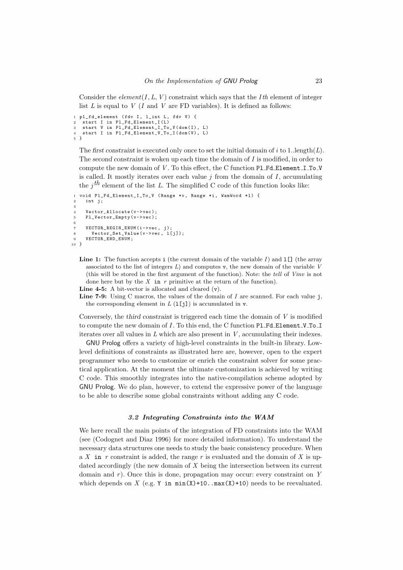
Consider the element(I ,L,V ) constraint which says that the I th element of integer
list L is equal to V (I and V are FD variables). It is defined as follows:
1 pl_fd_element (fdv I, l_int L, fdv V) {2 start I in Pl_Fd_Element_I(L)3 start V in Pl_Fd_Element_I_To_V(dom(I), L)4 start I in Pl_Fd_Element_V_To_I(dom(V), L)5 }
The first constraint is executed only once to set the initial domain of i to 1..length(L).
The second constraint is woken up each time the domain of I is modified, in order to
compute the new domain of V . To this effect, the C function Pl Fd Element I To V
is called. It mostly iterates over each value j from the domain of I , accumulating
the j th element of the list L. The simplified C code of this function looks like:
1 void Pl_Fd_Element_I_To_V (Range *v, Range *i, WamWord *l) {2 int j;3
4 Vector_Allocate(v->vec);5 Pl_Vector_Empty(v->vec);6
7 VECTOR_BEGIN_ENUM(i->vec , j);8 Vector_Set_Value(v->vec , l[j]);9 VECTOR_END_ENUM;
10 }
Line 1: The function accepts i (the current domain of the variable I ) and l[] (the arrayassociated to the list of integers L) and computes v, the new domain of the variable V(this will be stored in the first argument of the function). Note: the tell of Vinv is notdone here but by the X in r primitive at the return of the function).
Line 4-5: A bit-vector is allocated and cleared (v).Line 7-9: Using C macros, the values of the domain of I are scanned. For each value j,
the corresponding element in L (l[j]) is accumulated in v.
Conversely, the third constraint is triggered each time the domain of V is modified
to compute the new domain of I . To this end, the C function Pl Fd Element V To I
iterates over all values in L which are also present in V , accumulating their indexes.
GNU Prolog offers a variety of high-level constraints in the built-in library. Low-
level definitions of constraints as illustrated here are, however, open to the expert
programmer who needs to customize or enrich the constraint solver for some prac-
tical application. At the moment the ultimate customization is achieved by writing
C code. This smoothly integrates into the native-compilation scheme adopted by
GNU Prolog. We do plan, however, to extend the expressive power of the language
to be able to describe some global constraints without adding any C code.
3.2 Integrating Constraints into the WAM
We here recall the main points of the integration of FD constraints into the WAM
(see (Codognet and Diaz 1996) for more detailed information). To understand the
necessary data structures one needs to study the basic consistency procedure. When
a X in r constraint is added, the range r is evaluated and the domain of X is up-
dated accordingly (the new domain of X being the intersection between its current
domain and r). Once this is done, propagation may occur: every constraint on Y
which depends on X (e.g. Y in min(X)+10..max(X)+10) needs to be reevaluated.
24 D. Diaz, S. Abreu and P. Codognet
Doing so will potentially modify Y and all constraints depending on Y also need
to be reconsidered. The process finishes either when a failure occurs (the new do-
main of a variable is empty) or when a fix-point is reached (no more variables are
modified). In case of failure, Prolog backtracking occurs. It is then important to be
able to undo all modifications that have been done on the FD data structures.
Adding constraints over finite domains to the GNU Prolog WAM required the
introduction of a new term type (FD Variable, with the FDV tag) which, besides
contributing to tag space depletion, needs to be distinct from the regular REF term.
An FDV term has 2 distinct parts:
• Its domain: the set of allowable values, represented as the extrema of the con-
taining interval or as discrete individual values, encoded as a bitmap, possibly
multi-word. Using a bitmap greatly speeds up computation on sparse domains.
• The dependencies: the set of constraints which depend on the variable, i.e. those
which need to be recomputed each time the variable is modified. In order to op-
timize the triggering of these constraints, several distinct chains are maintained
(e.g. it is useless to re-execute a constraint depending on min(X ) when only
max (X ) is changed).
Classically, a value-trail mechanism is used to save an FD variable before its
modification (domain and/or dependencies). On backtracking, trailed values are
used to restore the FD variable. In order to avoid unnecessary trailings (for each FD
variable, at most one trailing is necessary per choice-point) a timestamp technique
is used: a sequential integer is used to number each choice-point and an FD variable
records the choice-point number associated to its last trailing. This is important
since FD variables are refined step by step by the propagation algorithms which
potentially compute several intermediate domains before reaching the fix-point.
The two parts of an FD variable (domain and dependencies) are generally not
modified at the same time during the execution of a constraint program. The depen-
dency chains are created and updated when the constraints are installed, typically
at the start of program execution, whereas the domains are more intensely modi-
fied later on, for instance during the labeling phase which tries to find a solution
through backtracking. For this purpose, each part of an FD variable (domain and
dependencies) maintains its own independent timestamp. In particular, when doing
labeling, we only trail the domain of the FD variables.
The other important data structure is the constraint frame, which stores the
information needed for constraint (re)evaluation. For an X in r primitive we need:
• A pointer to the constrained variable X .
• The address of the C function evaluating the range r (this is produced by fd2c
from the definition written in the constraint definition language).
• A pointer to the environment in which the function evaluating r executes: ba-
sically the function parameters, built by the constraint installation code.
We chose a dedicated stack in which to store all these data structures, called the
constraint stack. As for other Prolog data strucutures, the stack is used in back-
tracking: the top of the constraint stack is saved in choice-points and restored when
On the Implementation of GNU Prolog 25
backtracking occurs. This was not the case in clp(FD) where all FD data struc-
tures were located in the heap. In the tests we conducted, the performance impact
of having a constraint stack was negligible on programs which did not use FD.
From the above propagation algorithm it appears that the evaluation of a con-
straint leads to the reevaluation of other constraints. Theoretically, the order in
which constraints are woken up is not relevant (since the process stops when the
fix-point is reached). The easiest way to implement this consists of a depth-first
evaluation (recursively calling each constraint depending on the variable which has
just been updated). However, this blind recursive descent is not efficient in practice
and misses some important optimizations. It is thus better to explicitly handle a
queue of constraints. A first optimization consists of considering a queue of variables
instead of a queue of constraints. When a constraint needs to be reevaluated, it is as
consequence of the modification of some FD variable. It is easier to record just this
modified variable (a pointer) than to copy in the queue all depending constraints. In
GNU Prolog we go even further: the queue is not separately represented: instead, all
FD variables present in the queue are linked together. To this end, an FD variable
(see above) includes a third part which is devoted to the queue. It consists of:
• A link to the next enqueued variable (linked-list).
• A mask describing which dependencies need to be reconsidered (to avoid useless
reevaluations).
• A time-stamp to know whether a variable is already present in the queue. There
is a general counter which is incremented each time the (above) propagation
procedure is run. When a variable is modified, if its time-stamp is different from
the counter then the variable is not yet in the queue (it is then linked), otherwise
only its mask of dependencies is updated.
Note that our choice for the representation of the queue associated with the time-
stamp technique described above results in an optimization: the constraints depend-
ing on one variable are only present once in the queue. On a set of benchmarks, this
optimization saves an average 17% of the execution time (it is particularly effective
on arithmetic constraints) with no overhead. Detecting this case with a separate
queue would be much more time-consuming.
Another optimization which works well in practice for many constraints is that
an X in r primitive does not need to be evaluated if X has been instantiated
before the start of the propagation procedure. This can be detected reusing the
same counter described above. On some examples this optimizations saves up to
72% of the execution time (in particular when many disequalities are involved).
We have shown that GNU Prolog smoothly integrates an efficient FD solver,
proposing a simple yet powerful language in which to describe high-level constraints
and propagators. Those constraints are compiled down to C code, which in turn is
integrated into the GNU Prolog executable build flow of figure 1. More constraints
can then easily be added thanks to the description language and if needed with the
help of dedicated user-defined C functions. The compilation of high-level constraints
is based on a limited set of primitives which are well optimized. These optimizations
26 D. Diaz, S. Abreu and P. Codognet
are “general” (vs. “ad-hoc optimizations” of black-box solvers). So all high-level
constraints can benefit from them.
4 GNU Prolog and the Prolog Standard
From the outset, GNU Prolog has aimed to comply with common practice in Prolog
implementations, while retaining its characteristic architectural organization: to fit
into a regular native code compiler system, in which executables are produced by
linking object modules.
GNU Prolog was developed at the same time as the ISO Core 1 standard (ISO-
Part1 1995), which led us to take the standard proposal into account from the
outset. GNU Prolog therefore became the first Prolog system to closely comply with
the ISO standard. This meant supplying not only the standard built-in predicates
but also the related error behaviours (e.g. exceptions), the logical database update
view for dynamic predicates, meta-calls (the ISO standard requires a term to be
transformed into a goal before execution), directives, etc. 12
We took compatibility one step further by providing a classical Prolog top-level
interpreter, with all the expected facilities operational, including goal execution,
source display (the listing/0 predicate), a trace-mode 4-port debugger, program
consult and reconsult, Prolog state manipulation operations (character classifica-
tion, operator definitions, etc.) We do think that a top-level interpreter is a primitive
form of Integrated Development Environment (IDE): it makes historic sense, but
it would be better to integrate stripped-down compiler-like tools into a graphical
IDE such as Eclipse, NetBeans or Xcode by means of a plug-in.
It can be argued that the DEC-10 Prolog compiler was influential in many ways
and some aspects of its design persist in today’s Prolog systems. Its operating envi-
ronment set a model which would be emulated by most Prolog systems which came
thereafter: the interactive top-level with a “workspace” concept, which contains
the whole of the program, all seamlessly integrated, regardless of the representa-
tion used for Prolog code: clausal form suitable for a meta-interpreter, lower-level
instructions adapted to a byte-code interpreter or even executable native code.
This model holds, among others, for DEC-10 Prolog, C-Prolog, Quintus, SICStus,
MU-Prolog and Nu-Prolog, YAP, XSB, SWI, Ciao, BinProlog, ECLiPSe and B-
Prolog. With such a heritage, GNU Prolog was almost compelled to follow suit and
establish itself around the concept of a top-level interpreter managing goals executed
in the context of a dynamically-adjustable workspace, comprising all the Prolog
modules and equipped with a 4-port debugger, familiar to Prolog programmers,
although not strictly part of the language.
The functional enrichment of Prolog systems, and in particular those features
that stem from the language’s meta-programming capabilities, went forth basically
12 It is worth noting that GNU Prolog has kept up with the proposed revisions to the standard,including features such as call/N, conditional compilation directives and evaluable functors,among others.
On the Implementation of GNU Prolog 27
unaware of the distinction between “compile time” and “execution time” environ-
ments. This mingling is such that executing one query may influence a subsequent
consult operation, in ways that may completely alter its semantics (for instance,
operator definitions.)
For a system like GNU Prolog, which does independent static compilation to na-
tive code and clearly separates the compilation from the execution environments,
providing a top-level interpreter similar to other systems was a challenge which
required a large development effort. This requirement prompted the addition of a
bytecode emulator to GNU Prolog, similar to what is done in other Prolog imple-
mentations, to provide a not-too-inefficient means of implementing the culturally-
accepted development cycle for Prolog programs: edit/reconsult/run. The grief over
compile-time vs. runtime environments is not confined to GNU Prolog though: this is
a prominent issue in all systems that do static analysis or program transformation,
such as mode or type analyzers or even simple pretty-printers.
We feel that the ISO standard missed a good opportunity to disentangle this
situation and separate compile from execution environments. In particular:
1. The :- initialization directive was meant for an interpreted environment,
where one expects it to have an immediate effect on the rest of the program,
whether it is simply being compiled or actually being loaded. The semantics of
this directive are unclear when the driving goal is, for instance, something like
consult([f1, f2]), in which the initialization directives from f1 may influence
the loading of f2. A possible way around this issue is to separate the execution
of the initialization directives from the loading of the modules: GNU Prolog only
executes the initializers once all modules have been loaded. The execution order
is, in terms of the ISO standard, “implementation dependent.”
2. Another ISO directive which causes grief is multifile/1: one problem is the
order in which the multiple batches of clauses get collected. This is not an issue
in an interpreted environment, in which the loading is explicitly controlled by
the programmer whereas in a statically compiled set of Prolog files the order is
largely unpredictable, because it is left to the linker’s criteria.
3. One unfortunate feature of the Prolog language, legacy of the interpreter tradi-
tion, is the lack of distinction between code and data-only (database) dynamic
predicates. The ISO standard missed the opportunity to clearly distinguish be-
tween these two traditional uses for dynamic predicates: persistent data and
dynamic code manipulation.
These were but a few of the difficulties which hit us when developing GNU Prolog;
nevertheless, we strived to provide a fair rendering of an expected set of built-in
predicates. The “standard” Prolog library is nowhere near as complex as that of
other languages so the extent of this requirement is limited. We also behave con-
servatively w.r.t. extra-logical aspects of Prolog, such as the handling of directives.
28 D. Diaz, S. Abreu and P. Codognet
5 Conclusions and Directions for Future Work
We have presented the most significant aspects of the implementation of GNU Prolog
for which the key issues were simplicity, extensibility and maintainability without
sacrificing performance. This led us to the native-code generation approach which
has been described in this article. We applied the same requirements for the design
and the development of the finite domain constraint solver. One might say that,
overall, the GNU Prolog experience has been successful. The GNU Prolog “family”,
which includes wamcc and clp(FD) has been used in teaching and as the basis of
several extensions, most notably by other research teams: this fulfills one of our
design goals which was to establish a system sufficiently simple for it to be easily
extended by other people.
Several architectural ports and some extensions have been provided by the user
community, as acknowledged in the GNU Prolog distributed documentation. Mod-
ified versions of GNU Prolog have been used for prototyping systems, featuring
module systems, threads, attributed variables, CLP(R), RDBMS integration, Java
interfaces, a MacOSX IDE, to name but a few. The community-supplied extensions
are referenced on the main site at http://www.gprolog.org/#contribs.
In what concerns dissemination, the GNU Prolog distribution had been down-
loaded well over 100000 times from the development FTP site, over a period of
four years. We no longer keep statistics, as GNU Prolog is part of several Linux
distributions and there is no way to account for downloads from the main GNU
FTP site nor from other mirrors.
Performance-wise, GNU Prolog scores honorably, barely below YAP (da Silva and
Santos Costa 2006) which is continually being tuned for performance. We compared
GNU Prolog 1.4.0 and YAP 5.1.3 on 64-bit Linux. On the average, YAP is faster by
factor of 1.3 with peaks up to 2. However, on some benchmarks GNU Prolog can
outperform YAP by a factor of up to 1.4. With respect to wamcc we clearly gained
in usability, as a consequence of the more realistic compile times. GNU Prolog is
currently being worked on in various directions, including:
• Modules: GNU Prolog initially did not implement any module system, staying
within the bounds of ISO Prolog Core 1, awaiting the ISO Modules specification.
Reaching a consensus on modules took a long time and the resulting specifica-
tion is still not very satisfactory. We initially opted for the implementation of
a cleaner alternative mechanism, Contextual Logic Programming (Abreu and
Diaz 2003). Nevertheless, as there is a clear need for an interoperable module
system, we are finishing a minimal-functionality module system as part of the
Prolog Commons initiative, which brings GNU Prolog at par with the other
implementations.
• Other ISO Prolog Features: ISO compliance has been foremost in the design
and implementation of GNU Prolog; the work being carried out by the ISO
standization committee is being actively followed. For instance, one aspect that
needs to be accounted for is the handling of Unicode characters.
• Attributed Variables: even though GNU Prolog has a very efficient, conve-
nient and easily extensible FD constraint solver, it makes sense to include other
On the Implementation of GNU Prolog 29
constraint domains. Attributed variables are a mechanism which can be used to
effectively implement constraints and propagation over other domains.
• Tabling: using tabling allows one to write programs which are more expressive
because the system takes care of memoizing for us. More programs terminate
which would otherwise loop and this can be a very effective programming device.
This extension to Prolog was introduced in XSB (Rao et al. 1997) and has since
been included in other systems, namely YAP (Rocha et al. 2000; Rocha et al.
2005) and B-Prolog (Zhou et al. 2008).
• A Garbage Collector: GNU Prolog has gotten by without GC. While reason-
able for short-lived processes13 it is a limiting factor for larger executions.
• Improved Compiler: the GNU Prolog Prolog-to-WAM compiler is rather sim-
ple. This is an obvious area for improvements.
• Compilation Pipeline: because it is made up of a succession of filters, GNU
Prolog is amenable to the substitution of some of these: we are presently working
on a few, for instance one which manages EAM-style executions from the WAM
code. A longer-term goal is to rework the GNU Prolog back-end and improve its
integration into an existing compiler scheme: LLVM (Lattner and Adve 2004) is
an interesting target, as it is essentially a machine-independent, typed assembly
language which could take over the MA and Assembly language steps.
Acknowledgements: The authors wish to acknowledge the anonymous reviewers who
read early versions of this text and whose criticisms contributed to significantly
improve its form and substance.
References
Abreu, S. and Diaz, D. 2003. Objective: In minimum context. In ICLP, C. Palamidessi,Ed. Lecture Notes in Computer Science, vol. 2916. Springer, 128–147.
Aıt-Kaci, H. 1991. Warren’s Abstract Machine: A Tutorial Reconstruction. MIT Press.
Andre, P. and Abreu, S. 2010. Casting the WAM as an EAM. In Proceedings ofCICLOPS-WLPE 2010, G. Vidal and N.-F. Zhou, Eds.
Carlsson, M. 1990. Design and Implementation of an Or-Parallel Prolog Engine. Ph.D.thesis, SICS.
Chikayama, T., Fujise, T., and Sekita, D. 1994. A portable and efficient implemen-tation of kl1. In PLILP, M. V. Hermenegildo and J. Penjam, Eds. Lecture Notes inComputer Science, vol. 844. Springer, 25–39.
Codognet, P. and Diaz, D. 1995. Wamcc: Compiling prolog to c. In ICLP. 317–331.
Codognet, P. and Diaz, D. 1996. Compiling constraints in clp(fd). Journal of LogicProgramming 27, 3, 185–226.
da Silva, A. F. and Santos Costa, V. 2006. The design of the yap compiler: Anoptimizing compiler for logic programming languages. J. UCS 12, 7, 764–787.
Diaz, D. and Codognet, P. 1993. A minimal extension of the wam for clp(fd). In ICLP.774–790.
13 GNU Prolog is very suitable for building small executables, with short load times: Unix systemsshare code sections and this means code lingers even when no processes are using it. This isnormally not the case with bytecodes kept in writeable, non-shared memory.
30 D. Diaz, S. Abreu and P. Codognet
Ferreira, M. and Damas, L. 1999. Multiple specialization of wam code. In PADL,G. Gupta, Ed. Lecture Notes in Computer Science, vol. 1551. Springer, 243–258.
Gudeman, D., de Bosschere, K., and Debray, S. 1992. jc: An Efficient and PortableSequential Implementation of Janus. In Joint International Conference and Symposiumon Logic Programming. MIT Press, Washington, DC.
Hausman, B. 1993. Turbo erlang: Approaching the speed of c. In ICLP-Workshops onImplementation of Logic Programming Systems. 119–135.
Haygood, R. C. 1994. Native code compilation in sicstus prolog. In In Proceedings ofthe Eleventh International Conference on Logic Programming. MIT Press, 190–204.
ISO-Part1 1995. Information technology - Programming languages - Prolog - Par t 1:General Core. ISO/IEC 13211-1.
Jaffar, J. and Lassez, J.-L. 1987. Constraint logic programming. In POPL. 111–119.
Jones, S. L. P., Nordin, T., and Oliva, D. 1997. C--: A Portable Assembly Language.In Implementation of Functional Languages, C. Clack, K. Hammond, and A. J. T. Davie,Eds. Lecture Notes in Computer Science, vol. 1467. Springer, 1–19.
Lattner, C. and Adve, V. 2004. LLVM: a compilation framework for lifelong pro-gram analysis transformation. In Code Generation and Optimization, 2004. CGO 2004.International Symposium on. 75 – 86.
Rao, P., Sagonas, K., Swift, T., Warren, D., and Freire, J. 1997. XSB: A systemfor efficiently computing well-founded semantics. In Proceedings of the 4th InternationalConference on Logic Programming and Non-Monotonic Reasoning (LPNMR’97). Vol.1265. 2–17.
Rocha, R., Silva, F., and Santos Costa, V. 2000. YapTab: A tabling engine designedto support parallelism. In Conference on Tabulation in Parsing and Deduction. 77–87.
Rocha, R., Silva, F. M. A., and Costa, V. S. 2005. On applying or-parallelism andtabling to logic programs. TPLP 5, 1-2, 161–205.
Tsang, E. 1993. Foundations of Constraint Satisfaction. Academic Press.
Van Hentenryck, P. 1989. Parallel constraint satisfaction in logic programming: Pre-liminary results of chip within pepsys. In ICLP. 165–180.
Van Hentenryck, P., Saraswat, V. A., and Deville, Y. 1994. Design, implemen-tation, and evaluation of the constraint language cc(fd). In Constraint Programming,A. Podelski, Ed. Lecture Notes in Computer Science, vol. 910. Springer, 293–316.
Van Roy, P. and Despain, A. M. 1992. High-performance logic programming with theaquarius prolog compiler. IEEE Computer 25, 1, 54–68.
Warren, D. H. D. 1983. An Abstract Prolog Instruction Set. Technical Note 309, SRIInternational.
Zhou, N.-F., Sato, T., and Shen, Y.-D. 2008. Linear tabling strategies and optimiza-tions. TPLP 8, 1, 81–109.