on the k-mer frequency spectra of organism genome and

ON THE K-MER FREQUENCY SPECTRA OF

ORGANISM GENOME AND PROTEOME SEQUENCES

WITH A PRELIMINARY MACHINE LEARNING

ASSESSMENT OF PRIME PREDICTABILITY

by

Nathan O. Schmidt

A thesis

submitted in partial fulfillment

of the requirements for the degree of

Master of Science in Computer Science

Boise State University

August 2012

BOISE STATE UNIVERSITY GRADUATE COLLEGE

DEFENSE COMMITTEE AND FINAL READING APPROVALS

of the thesis submitted by

Nathan O. Schmidt

Thesis Title: On the k-mer frequency spectra of organism genome and proteomesequences with a preliminary machine learning assessment of prime predictability

Date of Final Oral Examination: 12 August 2012

The following individuals read and discussed the thesis submitted by student NathanO. Schmidt, and they evaluated his presentation and response to questions during thefinal oral examination. They found that the student passed the final oral examination.

Tim Andersen, Ph.D. Chair, Supervisory Committee

Amit Jain, Ph.D. Member, Supervisory Committee

Greg Hampikian, Ph.D. Member, Supervisory Committee

The final reading approval of the thesis was granted by Tim Andersen, Ph.D., Chair,Supervisory Committee. The thesis was approved for the Graduate College by JohnR. Pelton, Ph.D., Dean of the Graduate College.

ACKNOWLEDGMENTS

This thesis was supported by Dr. Tim Andersen and the United States Depart-

ment of Defense through the DNA Safeguard Project.

iii

ABSTRACT

A regular expression and region-specific filtering system for biological records

at the National Center for Biotechnology database is integrated into an object-

oriented sequence counting application, and a statistical software suite is designed

and deployed to interpret the resulting k-mer frequencies—with a priority focus on

nullomers. The proteome k-mer frequency spectra of ten model organisms and the

genome k-mer frequency spectra of two bacteria and virus strains for the coding and

non-coding regions are comparatively scrutinized. We observe that the naturally-

evolved (NCBI/organism) and the artificially-biased (randomly-generated) sequences

exhibit a clear deviation from the artificially-unbiased (randomly-generated) his-

togram distributions. Furthermore, a preliminary assessment of prime predictability

is conducted on chronologically ordered NCBI genome snapshots over an 18-month

period using an artificial neural network; three distinct supervised machine learning

algorithms are used to train and test the system on customized NCBI data sets to

forecast future prime states—revealing that, to a modest degree, it is feasible to make

such predictions.

iv

TABLE OF CONTENTS

ABSTRACT . . . . . . . . . . . . . . . . . . . . . . . . . . . . . . . . . . . . . . . . . . . . . . . iv

LIST OF TABLES . . . . . . . . . . . . . . . . . . . . . . . . . . . . . . . . . . . . . . . . . . x

LIST OF FIGURES . . . . . . . . . . . . . . . . . . . . . . . . . . . . . . . . . . . . . . . . . xiii

LIST OF ABBREVIATIONS . . . . . . . . . . . . . . . . . . . . . . . . . . . . . . . . . xv

1 Introduction . . . . . . . . . . . . . . . . . . . . . . . . . . . . . . . . . . . . . . . . . . . . . 1

1.1 Overview . . . . . . . . . . . . . . . . . . . . . . . . . . . . . . . . . . . . . . . . . . . . . . . . 1

1.2 Statement and Hypothesis . . . . . . . . . . . . . . . . . . . . . . . . . . . . . . . . . . . 3

1.3 Significance . . . . . . . . . . . . . . . . . . . . . . . . . . . . . . . . . . . . . . . . . . . . . . . 4

2 Background . . . . . . . . . . . . . . . . . . . . . . . . . . . . . . . . . . . . . . . . . . . . . 5

2.1 Overview . . . . . . . . . . . . . . . . . . . . . . . . . . . . . . . . . . . . . . . . . . . . . . . . 5

2.2 Literature Review . . . . . . . . . . . . . . . . . . . . . . . . . . . . . . . . . . . . . . . . . . 5

3 Implementation Phase . . . . . . . . . . . . . . . . . . . . . . . . . . . . . . . . . . . . 16

3.1 Overview . . . . . . . . . . . . . . . . . . . . . . . . . . . . . . . . . . . . . . . . . . . . . . . . 16

3.2 CSeq Application Enhancement . . . . . . . . . . . . . . . . . . . . . . . . . . . . . . . 16

3.2.1 Object-Oriented Sequence Iterator . . . . . . . . . . . . . . . . . . . . . . . 17

3.2.2 NCBI Data Stream Filtering . . . . . . . . . . . . . . . . . . . . . . . . . . . . 19

3.2.3 GeneSIS Cluster Optimizations . . . . . . . . . . . . . . . . . . . . . . . . . . 20

v

3.3 Statistical Analysis Applications . . . . . . . . . . . . . . . . . . . . . . . . . . . . . . 24

3.3.1 Rankseq: k-mer Arrangement and Classification . . . . . . . . . . . . 24

3.3.2 NcbiStat: Genome Sequence Summarization . . . . . . . . . . . . . . . 25

3.3.3 Genseq: Artificial Sequence Generation . . . . . . . . . . . . . . . . . . . 27

3.3.4 Freqseq: Identifying the k-mer Frequency Spectra . . . . . . . . . . . 27

3.3.5 Nullcountseq: Nullomer Set Cardinality and Intersection Ratio . 28

3.3.6 Predictseq: Prime Prediction . . . . . . . . . . . . . . . . . . . . . . . . . . . 29

3.3.7 Tdataformat: Predictseq Data Set Formatting . . . . . . . . . . . . . . 31

3.3.8 Tdatamerge: Predictseq Data Set Consolidation . . . . . . . . . . . . 32

3.3.9 34Seq: Nucleotide 3-mers, 4-mers, and GC Statistics . . . . . . . . . 33

3.3.10 SetStat: Default Accuracy and Prime Error Superset Reporting 34

3.4 Format and Display Applications . . . . . . . . . . . . . . . . . . . . . . . . . . . . . . 34

3.4.1 Rangestat: The Global Rankseq Range . . . . . . . . . . . . . . . . . . . 35

3.4.2 Histoseq: Histogram Compilation . . . . . . . . . . . . . . . . . . . . . . . . 36

3.4.3 Histoavg: Histogram Consolidation . . . . . . . . . . . . . . . . . . . . . . . 36

3.4.4 Scriptgen: Cluster Execution Script Generation . . . . . . . . . . . . . 37

4 Result and Analysis Phase . . . . . . . . . . . . . . . . . . . . . . . . . . . . . . . . . 38

4.1 Overview . . . . . . . . . . . . . . . . . . . . . . . . . . . . . . . . . . . . . . . . . . . . . . . . 38

4.2 A Preliminary k-mer Language . . . . . . . . . . . . . . . . . . . . . . . . . . . . . . . 38

4.2.1 Genetic Strings, Substrings, and k-mers . . . . . . . . . . . . . . . . . . . 38

4.2.2 Superregions, Regions, and Subregions . . . . . . . . . . . . . . . . . . . . 40

4.2.3 k-mers: Frequency, Boolean Observed State, and Probability . . . 42

4.3 Experiment 1: Organism k-mer Frequency Spectra and Nullomer Se-

quence Investigation . . . . . . . . . . . . . . . . . . . . . . . . . . . . . . . . . . . . . . . . 46

vi

4.3.1 Objective Summary . . . . . . . . . . . . . . . . . . . . . . . . . . . . . . . . . . 46

4.3.2 Ten Model Organism Results and Analysis . . . . . . . . . . . . . . . . . 47

4.3.3 Bacteria Strain Results: Escherichia coli . . . . . . . . . . . . . . . . . . 57

4.3.4 Virus Strain Results: Human immunodeficiency virus . . . . . . . . 65

4.4 Experiment 2: NCBI Genome Database Evolution and Time Series

Analysis: Prime Prediction Assessment . . . . . . . . . . . . . . . . . . . . . . . . . 71

4.4.1 Objective Summary . . . . . . . . . . . . . . . . . . . . . . . . . . . . . . . . . . 71

4.4.2 Training, Testing, and Prediction Results: The Artificial Neural

Network . . . . . . . . . . . . . . . . . . . . . . . . . . . . . . . . . . . . . . . . . . . . 71

5 Conclusion . . . . . . . . . . . . . . . . . . . . . . . . . . . . . . . . . . . . . . . . . . . . . . 80

5.1 Results Discussion . . . . . . . . . . . . . . . . . . . . . . . . . . . . . . . . . . . . . . . . . 80

5.1.1 Experiment 1 . . . . . . . . . . . . . . . . . . . . . . . . . . . . . . . . . . . . . . . 80

5.1.2 Experiment 2 . . . . . . . . . . . . . . . . . . . . . . . . . . . . . . . . . . . . . . . 82

5.2 Implication . . . . . . . . . . . . . . . . . . . . . . . . . . . . . . . . . . . . . . . . . . . . . . . 83

5.2.1 Experiment 1 . . . . . . . . . . . . . . . . . . . . . . . . . . . . . . . . . . . . . . . 83

5.2.2 Experiment 2 . . . . . . . . . . . . . . . . . . . . . . . . . . . . . . . . . . . . . . . 84

5.3 Future Exploration . . . . . . . . . . . . . . . . . . . . . . . . . . . . . . . . . . . . . . . . . 84

5.3.1 Experiment 1 . . . . . . . . . . . . . . . . . . . . . . . . . . . . . . . . . . . . . . . 84

5.3.2 Experiment 2 . . . . . . . . . . . . . . . . . . . . . . . . . . . . . . . . . . . . . . . 86

5.4 Recapitulation . . . . . . . . . . . . . . . . . . . . . . . . . . . . . . . . . . . . . . . . . . . . 87

REFERENCES . . . . . . . . . . . . . . . . . . . . . . . . . . . . . . . . . . . . . . . . . . . . . 89

A User Manual . . . . . . . . . . . . . . . . . . . . . . . . . . . . . . . . . . . . . . . . . . . . 93

A.1 Overview . . . . . . . . . . . . . . . . . . . . . . . . . . . . . . . . . . . . . . . . . . . . . . . . 93

vii

A.2 CSeq . . . . . . . . . . . . . . . . . . . . . . . . . . . . . . . . . . . . . . . . . . . . . . . . . . . . 93

A.2.1 Processor . . . . . . . . . . . . . . . . . . . . . . . . . . . . . . . . . . . . . . . . . . . 93

A.2.2 Reprocessor . . . . . . . . . . . . . . . . . . . . . . . . . . . . . . . . . . . . . . . . . 94

A.2.3 FASTA Filtering . . . . . . . . . . . . . . . . . . . . . . . . . . . . . . . . . . . . . 94

A.2.4 Genbank Filtering . . . . . . . . . . . . . . . . . . . . . . . . . . . . . . . . . . . . 94

A.3 Analysis Applications . . . . . . . . . . . . . . . . . . . . . . . . . . . . . . . . . . . . . . . 96

A.3.1 Rankseq . . . . . . . . . . . . . . . . . . . . . . . . . . . . . . . . . . . . . . . . . . . 96

A.3.2 NcbiStat . . . . . . . . . . . . . . . . . . . . . . . . . . . . . . . . . . . . . . . . . . . 96

A.3.3 Genseq . . . . . . . . . . . . . . . . . . . . . . . . . . . . . . . . . . . . . . . . . . . . 96

A.3.4 Freqseq . . . . . . . . . . . . . . . . . . . . . . . . . . . . . . . . . . . . . . . . . . . . 97

A.3.5 Nullcountseq . . . . . . . . . . . . . . . . . . . . . . . . . . . . . . . . . . . . . . . . 98

A.3.6 Predictseq . . . . . . . . . . . . . . . . . . . . . . . . . . . . . . . . . . . . . . . . . . 98

A.3.7 Tdataformat . . . . . . . . . . . . . . . . . . . . . . . . . . . . . . . . . . . . . . . . 98

A.3.8 Tdatamerge . . . . . . . . . . . . . . . . . . . . . . . . . . . . . . . . . . . . . . . . . 99

A.3.9 34Seq . . . . . . . . . . . . . . . . . . . . . . . . . . . . . . . . . . . . . . . . . . . . . . 99

A.3.10 Setstat . . . . . . . . . . . . . . . . . . . . . . . . . . . . . . . . . . . . . . . . . . . . . 99

A.4 Format and Display Applications . . . . . . . . . . . . . . . . . . . . . . . . . . . . . . 99

A.4.1 Rangestat . . . . . . . . . . . . . . . . . . . . . . . . . . . . . . . . . . . . . . . . . . 99

A.4.2 Histoseq . . . . . . . . . . . . . . . . . . . . . . . . . . . . . . . . . . . . . . . . . . . 99

A.4.3 Histoavg . . . . . . . . . . . . . . . . . . . . . . . . . . . . . . . . . . . . . . . . . . . 100

A.4.4 Scriptgen . . . . . . . . . . . . . . . . . . . . . . . . . . . . . . . . . . . . . . . . . . . 100

B Source Code Snippets . . . . . . . . . . . . . . . . . . . . . . . . . . . . . . . . . . . . . 102

B.1 Overview . . . . . . . . . . . . . . . . . . . . . . . . . . . . . . . . . . . . . . . . . . . . . . . . 102

B.2 Analysis Applications . . . . . . . . . . . . . . . . . . . . . . . . . . . . . . . . . . . . . . . 102

viii

C Detailed Experimentation Procedures . . . . . . . . . . . . . . . . . . . . . . . 104

C.1 Overview . . . . . . . . . . . . . . . . . . . . . . . . . . . . . . . . . . . . . . . . . . . . . . . . 104

C.2 Experiment 1 . . . . . . . . . . . . . . . . . . . . . . . . . . . . . . . . . . . . . . . . . . . . . 104

C.2.1 Preparation . . . . . . . . . . . . . . . . . . . . . . . . . . . . . . . . . . . . . . . . . 104

C.2.2 Procedure . . . . . . . . . . . . . . . . . . . . . . . . . . . . . . . . . . . . . . . . . . 105

C.3 Experiment 2 . . . . . . . . . . . . . . . . . . . . . . . . . . . . . . . . . . . . . . . . . . . . . 107

C.3.1 Preparation . . . . . . . . . . . . . . . . . . . . . . . . . . . . . . . . . . . . . . . . . 107

C.3.2 Procedure . . . . . . . . . . . . . . . . . . . . . . . . . . . . . . . . . . . . . . . . . . 108

D Graphical Results . . . . . . . . . . . . . . . . . . . . . . . . . . . . . . . . . . . . . . . . 111

D.1 Overview . . . . . . . . . . . . . . . . . . . . . . . . . . . . . . . . . . . . . . . . . . . . . . . . 111

D.2 AA k-FS Results: Apis mellifera Example . . . . . . . . . . . . . . . . . . . . . . . 111

ix

LIST OF TABLES

4.1 The ten model organism’s AA k-FS analysis configuration . . . . . . . . . . 50

4.2 The ten model organism’s AA k-FS data sets. The total sequence

length |S| is used for the Genseq’s “generation size” . . . . . . . . . . . . . . . 50

4.3 The ten model organism’s AA 4-nullomer set cardinality and intersec-

tion ratio comparisons for statistics with length-3 subsequence parti-

tioning . . . . . . . . . . . . . . . . . . . . . . . . . . . . . . . . . . . . . . . . . . . . . . . . . . 51

4.4 The ten model organism’s AA 5-nullomer set cardinality and intersec-

tion ratio comparisons for statistics with length-3 subsequence parti-

tioning . . . . . . . . . . . . . . . . . . . . . . . . . . . . . . . . . . . . . . . . . . . . . . . . . . 51

4.5 The ten model organism’s AA 5-nullomer ranking histogram chi-square

comparisons for statistics with length-3 subsequence partitioning . . . . . 52

4.6 The ten model organism’s 3-FS, 4-FS, and 5-FS histogram chi-square

comparisons for the [0, 10000] frequency spectral-range . . . . . . . . . . . . . 53

4.7 The analysis summary of the ten model organism 3-FS distributions

in Figures 4.1, 4.2, 4.3, 4.4, and 4.5 . . . . . . . . . . . . . . . . . . . . . . . . . . . . 54

4.8 The EC bacteria’s DNA k-FS analysis configuration . . . . . . . . . . . . . . . 59

4.9 The EC bacteria’s DNA sequence data sets. Here, the superregion

length |Rτ | is used as Genseq’s “generation size” . . . . . . . . . . . . . . . . . . 60

4.10 The EC bacteria’s DNA 8-nullomer set cardinality comparisons for

statistics with length-7 subsequence partitioning . . . . . . . . . . . . . . . . . . 60

x

4.11 The EC bacteria’s DNA 8-nullomer set intersection ratio comparisons

for statistics with length-7 subsequence partitioning . . . . . . . . . . . . . . . 60









4.16 The EC bacteria’s DNA 10-nullomer ranking histogram chi-square com-

parisons for statistics with length-7 subsequence partitioning . . . . . . . . 62

4.17 The analysis summary of the EC bacteria 5-FS distributions in Figures

4.6 and 4.7 . . . . . . . . . . . . . . . . . . . . . . . . . . . . . . . . . . . . . . . . . . . . . . . 63

4.18 The HIV’s DNA/RNA k-FS analysis configuration . . . . . . . . . . . . . . . . 67

4.19 The HIV’s DNA/RNA sequence data sets. Here, the superregion

length |Rτ | is used as Genseq’s “generation size” . . . . . . . . . . . . . . . . . . 68

4.20 The HIV’s DNA/RNA 5-nullomer set cardinality and intersection ratio

statistical comparisons with length-3 subsequence partitioning . . . . . . . 68


statistical comparisons . . . . . . . . . . . . . . . . . . . . . . . . . . . . . . . . . . . . . . 68


statistical comparisons . . . . . . . . . . . . . . . . . . . . . . . . . . . . . . . . . . . . . . 68

4.23 Rankseq’s HIV DNA/RNA 7-nullomer probability histogram chi-square

comparisons with length-3 subsequence partitioning . . . . . . . . . . . . . . . 69

xi

4.24 The analysis summary of the HIV 3-FS distributions in Figures 4.8

and 4.9 . . . . . . . . . . . . . . . . . . . . . . . . . . . . . . . . . . . . . . . . . . . . . . . . . . 69

4.25 The size statistics for the balanced NCBI data set snapshots . . . . . . . . . 73

4.26 The size statistics for the unbalanced NCBI data set snapshots . . . . . . . 74

4.27 The ANN training configuration for the observed prime state predic-

tions on the monthly NCBI database snapshots . . . . . . . . . . . . . . . . . . . 78

4.28 The ANN training accuracies for 16-prime state prediction on the

balanced monthly DNA data sets ranging from January 2010 to July

2011 . . . . . . . . . . . . . . . . . . . . . . . . . . . . . . . . . . . . . . . . . . . . . . . . . . . . 78

4.29 Predictseq’s ANN prediction accuracies for the 16-prime state unbal-

anced monthly DNA data sets ranging from February 2010 to July

2011. We see that Predictseq’s accuracy Λtotal outperformed the ran-

dom biased guessing ΛBRG in 1416

cases. . . . . . . . . . . . . . . . . . . . . . . . . . . 79

xii

LIST OF FIGURES

4.1 Apis mellifera vs. Bos taurus: The ΓSHoneybee3 and ΓSCattle3 comparison

with a frequency spectral-range [0, 10000] for N data sets (only [0, 200]

is shown) . . . . . . . . . . . . . . . . . . . . . . . . . . . . . . . . . . . . . . . . . . . . . . . . 54

4.2 Canis familiaris vs. Gallus gallus: The ΓSDog3 and ΓSChicken3 comparison

with a frequency spectral-range [0, 10000] for the N data sets (only

[0, 200] is shown) . . . . . . . . . . . . . . . . . . . . . . . . . . . . . . . . . . . . . . . . . . 55

4.3 Danio rerio vs. Stronglyocentrus purpuratus: The ΓSZebrafish3 and ΓSSeaUrchin3

comparison with a frequency spectral-range [0, 10000] for the N data

sets (only [0, 200] is shown) . . . . . . . . . . . . . . . . . . . . . . . . . . . . . . . . . . 55

4.4 Homo sapien vs. Pan troglodytes: The ΓSHuman3 and ΓSChimp3 comparison

with a frequency spectral-range [0, 10000] for the N data sets (only

[0, 200] is shown) . . . . . . . . . . . . . . . . . . . . . . . . . . . . . . . . . . . . . . . . . . 56

4.5 Mus musculus vs. Rattus norvegicus: The ΓSMouse3 and ΓSRat3 compari-

son with a frequency spectral-range [0, 10000] for the N data sets (only

[0, 200] is shown) . . . . . . . . . . . . . . . . . . . . . . . . . . . . . . . . . . . . . . . . . . 56

4.6 EC-536: The DNA ΓSEC−536

5 region comparison with a frequency spectral-

range [0, 10000] for the N data sets (only [0, 200] is shown) . . . . . . . . . . 63

4.7 EC-55989: The DNA ΓSEC−55989

5 region comparison with a frequency

spectral-range [0, 10000] for the N data sets (only [0, 200] is shown) . . . 64

xiii

4.8 HIV-1: The DNA/RNA ΓSHIV−1


spectral-range [0, 300] for the N data set (only [0, 20] is shown) . . . . . . . 70

4.9 HIV-2: The DNA/RNA ΓSHIV−2


spectral-range [0, 300] for the N data set (only [0, 20] is shown) . . . . . . . 70

4.10 The FASTA DNA monthly NCBI datbase sizes ranging from January

2010 to July 2011 . . . . . . . . . . . . . . . . . . . . . . . . . . . . . . . . . . . . . . . . . . 75

4.11 The DNA 16-prime set cardinalities for the NCBI database snapshots

ranging from January 2010 to July 2011 . . . . . . . . . . . . . . . . . . . . . . . . 76

4.12 The DNA 16-prime set sizes (in megabytes) for the NCBI ANN training

and testing data sets ranging from January 2010 to July 2011 . . . . . . . . 77

4.13 A depiction of the ANN 16-prime state prediction accuracies for the

(unbalanced) monthly DNA data sets ranging from February 2010 to

July 2011 . . . . . . . . . . . . . . . . . . . . . . . . . . . . . . . . . . . . . . . . . . . . . . . . 79

B.1 Rankseq’s sequence probability ranking algorithm . . . . . . . . . . . . . . . . . 103

D.1 The honey bee’s length-5 AA nullomer ranking histogram for the NCBI

data set . . . . . . . . . . . . . . . . . . . . . . . . . . . . . . . . . . . . . . . . . . . . . . . . . 111

D.2 The honey bee’s length-5 AA nullomer ranking histogram for the length-

1 statistically generated data set . . . . . . . . . . . . . . . . . . . . . . . . . . . . . . . 112





D.5 The honey bee’s length-5 AA nullomer ranking histogram for the ran-

domly generated data set . . . . . . . . . . . . . . . . . . . . . . . . . . . . . . . . . . . . 114

xiv

LIST OF ABBREVIATIONS

DNA – Deoxyribonucleic acid

AA – Amino acid

NCBI – National Center for Biotechnology Information

k-FS – k-mer frequency spectra

HIV – Human immunodeficiency virus

EC – Escherichia coli

ANN – Artificial neural network

RAM – Random access memory

PVFS – Parallel Virtual File-System

xv

1

CHAPTER 1

INTRODUCTION

1.1 Overview

The k-mer frequency spectra (k-FS) is the set of all short-length words resident to

a genome or proteome, where each k-mer is mapped to an occurrence frequency.

Upon sequencing, organism sequences are digitized and stored at the National Center

for Biotechnology Information (NCBI) as FASTA and Genbank records to promote

computational examination. The sequence studies of [26, 7, 8] reveal a non-linear

variation in the genome distribution of these frequencies on a multitude of model

organism species; while some k-mers enjoy an occurrence plethora, others remain

absent. The minimum-length sequences that are absent from an organism are termed

nullomers and those that are absent from nature are termed primes. Are there

interesting proteome k-FS and nullomer properties? Can statistical distinctions be

made between the genome k-FS and nullomers of complete, coding, and non-coding

regions? In terms of the k-FS and nullomers, are the natural data sets of specific

organisms distinct from the artificial generated? If so, to what degree? As the

advances in bio-technology continue to yield a faster genome and proteome sequencing

rate, the total size of the NCBI database accelerates. So how might this rapid

technological expansion influence the prime phenomena? Is it possible to train an

intelligent system to analyze the NCBI database and forecast future prime states?

2

We investigate the k-FS properties for various subject organisms, with a priority-focus

on the nullomer/prime phenomena in terms of ranking and predictability.

In Chapter 2, we highlight the literature that influences this thesis and discuss

how these fundamental concepts direct our investigation.

In Chapter 3, we introduce the statistical software application suite that is de-

signed to instrument the k-mer-based sequence analysis. First, we present structural

and algorithmic enhancements to our core sequence processing utility, in terms of (1)

the GeneSIS cluster space and run-time optimizations, (2) the new object-oriented

iterator implementation, and (3) the logic-oriented sequence filtering sub-system.

Second, we discuss the purpose and key components to each individual application.

Third, we explain how the NCBI genomes and proteome data sets are processed,

interpreted, and evaluated by our software to statistically analyze the subject k-FS

and nullomers/primes.

In Chapter 4, we discuss the two distinct categories of experiments. In Experiment

1, the k-FS analysis, the natural data set frequency statistics are systematically com-

pared against those of the artificially-generated data sets (including randomly-biased

and randomly-unbiased) to determine the degree (if any) of similarity. First, we

examine the proteome of ten distinct model organisms to determine the amino acid

(AA) k-FS statistics. Second, we examine the genome of two Escherichia coli (EC)

strains and two Human immunodeficiency virus (HIV) strains, where we use our

sequence filtering sub-system to determine the deoxyribonucleic acid (DNA) k-FS

statistics for the complete, coding, and non-coding regions. In Experiment 2, the

prime prediction assessment, the month-by-month time-series evolution of the NCBI

database is chronologically analyzed by an artificial neural network (ANN); the ANN

is trained using three distinct machine learning techniques and used to forecast future

3

prime states.

In Chapter 5, we summarize this research, discuss implications, and suggest future

projections along this mode of bio-informatics exploration.

1.2 Statement and Hypothesis

In [26], Hampikian and Andersen introduce a publicly available algorithm for identi-

fying absent sequences and demonstrate its use by reporting the smallest k-mers not

found in NCBI’s organism genome database. These nullomers define the maximum set

of potentially lethal k-mers. Additional k-mer studies of complete organism genome

sequences have identified a non-linear variation in the frequency distribution using

statistical analysis software [7, 8]. The modalities of the k-FS distributions range

from uni-modal to multi-modal, generally depending on whether the organism is a

eukaryote or prokaryote. This series of experiments suggests evidence of deterministic

k-mer structure in complete organism genome sequences. This thesis seeks knowledge

of the k-FS and nullomer/prime phenomena by answering the following inquiries:

1. Experiment 1: Do the DNA and AA k-FS of the subject organisms exhibit

evidence of (1) structural bias or (2) are they completely random? How do the

nullomer set cardinalities and overlap (intersection) ratios comparatively differ

between the natural and artificial data sets?

2. Experiment 2: Does the time-dependent evolution of the NCBI database enable

us to predict future prime states? If so, to what degree of accuracy?

Our research tests a distinct hypothesis for both experiments. Our hypothesis for

1. Experiment 1 is: the k-FS for the selected subject organisms is non-random and

will therefore exhibit structural bias ; and

4

2. Experiment 2 is: the future prime states are inherently unpredictable (due to, for

example, an insufficient amount of genome information housed at NCBI, and the

unattainable degree of influential factors to consider, such as the environment,

the organisms, and the order of NCBI submission content).

1.3 Significance

The knowledge obtained from the results of this thesis may help establish a rational

basis for species identification, environmental characterization, genetic engineering,

and could someday prove useful to fields such as medicine. If science can develop

a fundamental understanding of the k-FS and nullomer/prime phenomena, then

perhaps someday it may be possible to identify the physical, chemical, and biological

mechanisms, or natural “algorithms” responsible for genetic mutations.

5

CHAPTER 2

BACKGROUND

2.1 Overview

In this chapter, we summarize the background literature that forms the foundation of

this thesis and explain how these concepts influenced this k-mer research deployment.

2.2 Literature Review

In [7], evolutionary features based on k-FS distributions of various organisms are

analyzed. There are three distinct groups based on their evolutionary periods, where

each category exhibits a distinct modality:

1. E. coli and T. pallidum: unimodal;

2. yeast, zebrafish, A. thaliana, and fruit fly: unimodal with peaks generally

shifted to smaller frequencies of occurrence; and

3. mouse, chicken, and human: bimodal.

Furthermore, a model based on the DNA cytosine-guanine “CG” content is introduced

and shown to provide reasonable agreements with the data.

In [8], the empirical frequencies of DNA k-mers in complete genome sequences

provide a distinct and interesting perspective on genome structure. More than 100

6

species from Archea, Bacteria, and Eukaryota are investigated, with a focus on

the k-FS modalities. They found that a few species, including all mammals, have

multimodal spectra (these species coincide with the tetrapods) and discovered that

low-order Markov models capture this property fairly well. The multimodal spectra

are characterized by specific ranges of values of C+G content and of CpG dinucleotide

suppression, a range that encompasses all tetrapods analyzed. Other genomes, like

that of the protozoa Entamoeba histolytica, which also exhibits CpG suppression, do

not have multimodal k-FS. Groupings of functional elements of the human genome

also have a clear modality, and exhibit either a unimodal or multimodal behaviour,

depending on the two above mentioned values.

In [26], a novel algorithm for identifying nullomers is introduced, where the authors

use it on NCBI Genbank records to report nullomer statistics for various model

organisms. They demonstrate that nullomers and primes provide a rational basis

for selecting artificial DNA sequences for molecular barcodes and may provide insight

into environmental characterization, antibiotic development, species identification,

comparative genomics, and potential target identification for therapeutic intervention.

It is shown that nullomers and primes can be used to delineate between the set of

natural and potentially unused sequences, where the boundary nullomers surround

various branches of the phylogenetic tree of life.

In [1], the authors demonstrate that the hypermutability of CpG dinucleotides,

rather than natural selection against nullomers, is likely the reason for the nullomer

phenomena. They investigate various human, chimpanzee, cow, dog, and mouse

genome instances. They observe that for these species, nullomers differ by only one

nucleotide, which suggests that mutation, rather than natural selection, is responsible

for the nullomer evolution and nullomer generation in species populations.

7

In [20], the authors present correlation analysis results of k-mer presence/absence

distributions ranging from 5 to 20 in more than 1500 microbial and virus genomes,

along with five multicellular organisms (including human). For organisms that are

not close relatives, the genome k-mer distributions are not correlated, but for close

biological relatives, some correlation is observed, but is not as strong as expected.

The results suggest that suppressed correlations of various genome n-mers leads to the

possibility of using random n-mer sets to discriminate genomes of different organisms

and possibly individual genomes of the same species, including human, with a low

error probability.

In [27], the authors demonstrate how a number of sequence comparison tasks can

be accomplished efficiently without an alignment step. This procedure is based on the

shortest unique substrings. These are k-mers that only occur once within the sequence

or set of sequences analyzed and that cannot be further reduced in length without

losing the uniqueness property. They report that the shortest unique substrings in C.

Elegans, human, and mouse are no longer than 11 base pairs in the autosomes of these

organisms. In mouse and human, these unique substrings are significantly clustered

in upstream regions of known genes. They derive an analytical expression for the

nullomer distribution of the shortest unique substrings, based on the GC-content of

the query sequences and apply this method to the rapid detection of unique genomic

regions in various bacteria strains.

In [23], the authors examine the relative abundances of dinucleotides and their

biases in various eukaryotic genomes and chromosomes, including human chromo-

somes 21 and 22, Saccharomyces cerevisiae, Arabidopsis thaliana, and Drosophila

melanogaster. They report that the dinucleotide relative abundances are remarkably

constant across human chromosomes and within the DNA of a particular species.

8

Moreover, the dinucleotide biases differ between species, and provide a genome sig-

nature that is characteristic of an organism’s DNA.

In [39], the authors report that the CpG dinucleotide is present at approximately

20% of its expected frequency in vertebrate genomes. They examine the hypothesis

that the 20% frequency represents an equilibrium between the rate of creation of

new CpGs and the accelerated rate of CpG loss from methylation. From this, they

calculate the expected reduction in the CpG equilibrium frequency and find that

the observed CpG deficiently can be explained by mutation from methylated CpG

to TpG/CpA at approximately 12 times the normal transition rate, the exact rate

depending on the ratio of transitions to transversions. This indicates that it would

take 25 million years or less, a small fraction of the time for vertebrate evolution, for

CpG frequency to be reduced from undepleted levels to the current depleted levels.

In [36], the authors compare various studies on the exact distribution of word

counts in random sequences in terms of approximation accuracy and computational

cost. They propose rules for choosing between the Gaussian approximations, com-

pound Poisson approximation, and exact distribution. They apply these concepts to

the detection of exceptional words in the phage Lambda genome.

In [35], the authors provide an overview based on the statistical and probabilistic

properties of words, as occurring in the analysis of biological genomes, where they

distinguish between various word frequencies and exact distributions as well as the

derivation of various approximation methods. They model a sequence as a stationary

ergodic Markov chain. A test is proposed for determining the appropriate order of

the representative Markov chain.

In [31], the authors aim to characterize protein databases, where they engage in

a systematic attempt to reveal protein database characters that could contribute to

9

revealing how protein chains are constructed. For this, they focus on using the set

of all the possible 3-mer, 4-mer, and 5-mer frequency distribution combinations. The

results suggest that these 3D information structures are protein functions that exist

in the context of short constituent sequence connections, which are reflected on their

availability differences in the database. These results may have biological implications

for protein structural studies.

In [40], the authors demonstrate that there are thousands of penta-peptides that

are absent from all known proteomes, but many of them are coded for multiple times

in the non-coding genomic regions. This suggests a strong selection process that

prevents these peptides from being expressed. They show that the characteristics of

these forbidden penta-peptides vary among various phylogenetic groups, where they

claim to provide the first steps toward understanding the grammar of the forbidden

penta-peptides.

In [19], the authors identify and investigate a large population of pseudogenes

in four sequenced eukaryotic genomesthe worm, yeast, fly, and human (chromo-

somes 21 and 22 only). Each of the 2500 pseudogenes is characterized by one

or more disablements, such as premature stops and frameshifts. They conduct a

comprehensive frequency survey of the amino acid and nucleotide composition in

these non-functional genes and compare them to functional genes and intergenic

DNA. They correlate the pseudogene amino acid composition to the intermediate

composition between genes and translated intergenic DNA. They establish that the

pseudogene intermediate composition applies even though the gene composition in

the four organisms is markedly different, showing a strong correlation with the overall

A/T content of the genomic sequence. They classify pseudogenes into ancient and

modern subsets, where modern pseudogenes typically exhibit a much closer sequence

10

composition to genes than ancient pseudogenes. Altogether, their results indicate that

the composition of pseudogenes that are not under selective constraints progressively

drift from that of coding DNA towards non-coding DNA. Therefore, they propose

that the degree to which pseudogenes approach a random sequence composition may

be useful in dating different sets of pseudogenes, as well as to assess the rate at which

intergenic DNA accumulates mutations.

In [22], the authors analyze the amino acid frequency distribution in seven nuclearly-

encoded and five mitochondrial-encoded inner membrane proteins. They establish

that the mitochondrially encoded proteins have many more positively charged residues

in their non-translocated, as compared to their translocated, domains. However,

most of the nuclearly-encoded proteins do not show such a bias, but instead have

a surprisingly skewed distribution of Glu residues. These results suggest that some,

but possibly not all, nuclearly-encoded proteins may insert into the membrane by a

mechanism that does not depend on the frequency distribution of positively charged

amino acids.

In [30], the authors investigate the frequency and binding of short linear motifs

(peptides of lengths three to eight) in terms of protein interaction networks. Their

objective is to explain how one protein is able to bind to very different partners. The

fact that they often reside in disordered regions in proteins makes them difficult to

detect through sequence comparison or experiment. So they demonstrate that binding

motifs can be detected using data from genome-scale interaction studies, which avoids

the normally slow discovery process in proteome-scale interactions. They focus on

motif over-representation in non-homologous sequences, rediscovering known motifs,

and predicting dozens of others. Of the predicted, direct-binding experiments reveal

that two motifs are indeed protein-biding modules. They estimate that there may be

11

dozens or even hundreds of linear motifs yet to be discovered that will give molecular

insight into protein networks and greatly illuminate cellular processes.

In [34], the authors propose an amino acid k-string frequency analysis as a sys-

tematic way of inferring evolutionary relatedness of microbial organisms from the

oligopeptide content. Their method contains only one parameter, the length k of the

oligopeptides, and therefore avoids the ambiguity of choosing the genes for phyloge-

netic reconstruction and variable length sequence alignment. This method is applied

to a total of 109 organisms, including 16 Archaea, 87 Bacteria, and 6 Eukarya, and

yields an unrooted tree that agrees with the biologists phylogenetic “tree of life,” based

on basic branching majorities on SUU rRNA. The tree-based topology converges with

k increasing.

In [41], the authors provide a novel method for efficient reconstruction of phy-

logenetic trees, based on complete genome and proteome sequences, whose lengths

may vary greatly. The technique measures the pairwise distances between sequences,

which is based on computing the average lengths of the maximum common substrings.

They propose an algorithm on suffix arrays for efficiently computing these distances

in O(k) time, where k in sequence length. An initial analysis of the results exhibits a

remarkable agreement with accepted phylogenetic and taxonomic truth. They discuss

five distinct applications of the method, which suggests a number of novel phylogenetic

insights.

In [6], the authors describe a hidden markov model used for detecting local

correlations in protein sequence structures based on the I-sites library. The model

is unlike the linear hidden Markov models because it employs a highly branched

topology and captures recurrent local features of protein sequences and structures to

predict protein secondary structure. The model achieves an accuracy of 74.3% and

12

recognizes a considerably higher probability to coding sequence regions. They suggest

that these methods will be useful for tertiary structure prediction.

In [16], the authors propose a chaos game representation to display short oligonu-

cleotide sequences in genomes in the form of fractal images. These images are

considered as a genomic signature. They demonstrate that short fragments of genomic

sequences retain most of the characteristics of the species they come from, and suggest

that it is possible to perform a global species comparison by using genome fragments

found in databases. They evaluate the efficiency of this approach as a function of the

fragment size and the oligonucleotide length.

In [5], the authors investigate the relative abundance functional for lengths 2, 3,

and 4 nucleotides in a broad phylogenetic range to discern tendencies and anomalies

in the frequency occurrences of these oligonucleotides. They find that for dinu-

cleotides, TA is almost universally under-represented, with the exception of verte-

brate mitochondrial genomes, and CG is strongly under-represented in vertebrates

and in mitochondrial genomes. Moreover, for trinucleotides, GCATGC tends to be

under-represented in phage, human viral, and eukaryotic sequences, and CTATAG

is strongly under-represented in many prokaryotic, eukaryotic, and viral sequences.

They consider various explanations for the over- and under- representations in terms

of DNA/RNA structures and regulatory mechanisms are considered.

In [4], the authors seek to understand how amino acid composition of proteins

has changed over the course of evolution. In doing so, they introduce a method

and simulation for estimating the composition of proteins in an ancestral genome.

The estimates are based upon the composition of conserved residues in descendant

sequences, and the relative probability of conservation in various amino acids. Rel-

ative to the modern protein set, the ancestral protein set was found to be generally

13

richer in those amino acids that are believed to have been most abundant in the

prebiotic environment and poorer in those amino acids that are believed to have been

unavailable or scarce. They propose that the inferred amino acid composition of

ancestral proteins reflects historical events in the establishment of the genetic code.

In [24], the author compares representative genomes from each of the three king-

doms of life in terms of protein structure, with a focus on a bacteria, an archaeon, and

yeast. This comparison is a frequency analysis of secondary and tertiary structures in

the genomes. The author discusses the similarities and differences between the data

sets in terms of degree of duplication, degree of overlap, the number of protein folds,

and the most common short-length strands. From these results, the author suggests

that the last common ancestor correlations to the three kingdoms are the most basic

molecular parts, including the TIM-barrell, Rossman avodoxin, thiamin-binding, and

P-loop hydrolase folds.

In [17], the authors explored genome DNA structures by means of a new tool

derived from chaotic dynamical systems theory, which allows them to depict oligonu-

cleotide frequencies as images. They observe that the subsequences of a genome

exhibit the main characteristics of the complete genome, reinforcing the validity of

the genome signature concept. The main factors explaining the observed sequence

variability are due to base concentrations, stretches (of complementary bases), and

patches (of over- or under-represented words of varying lengths). They demonstrate

that the distance between images may be considered a measure of phylogenetic

proximity, where eukaryotes and prokaryotes can be identified merely on the basis

of their DNA structures.

In [37], the authors establish that the rates and patterns of evolution at silent sites

in codons reveal much about the basic features of molecular evolution. They found

14

that for recent increases in the amount of sequence data available for various species

and more precise knowledge of the chromosomal locations of those sequences, coming

in particular from genome projects, reveal that some features of molecular evolution

vary around the genome.

In [18], the authors report two Chaos Game Representation (CGR) algorithms

that can predict the presence or absence of a stretch of nucleotides in any gene

family. They explain how the CRG can recognize patterns in nucleotide sequences

of a class of genes using the techniques of fractal structures and by considering DNA

sequences. These algorithms can provide a mathematical basis of the CGR patterns

obtained using nucleotide sequences from genome databases.

In [21], the author compares the trinucleotide frequencies in long sequences and

their shuffled counterparts. A frequency hierarchy is observed among the 32 com-

plementary trinucleotide pairs, which is influenced both by base composition (not

affected by shuffling the order of the bases) and by base order (affected by shuffling).

The author observes that the influence of base order is greatest in DNA with a GC-

content of of 50 percent and appears to reflect a more fundamental hierarchy of dinu-

cleotide frequencies. Therefore, if TpA is at low frequency, all eight TpA-containing

trinucleotides are at low frequency. Moreover, the author reports that mammals

and their viruses share similar hierarchies, with genomic differences being generally

associated with differences in base composition (percentage of GC content). E. coli

and, to a lesser extent, Drosophila melanogaster hierarchies differ from mammalian

hierarchies; this is associated with differences both in base composition and in base

order. Therefore, the author proposes that Chargaff’s rule applies to single-stranded

DNA because there has been an evolutionary selection pressure favoring mutations

that generate complementary oligonucleotides in close proximity, thus creating a

15

potential to form stem-loops. These are dispersed throughout genomes and are

rate-limiting in recombination. These results suggest that GC-content delineations

between species would impair interspecies recombination by interfering with stem-loop

interactions.

In [10, 9, 14, 12, 11, 13, 32, 25], the authors investigate low-frequency vibrations

in biomacromolecules. They explain that these structures possess significant biolog-

ical functions. They demonstrate that biomolecule helices generate low frequency

collective vibrations in the form of phonons.

In [3], the authors reveal a parametric resonance in DNA dynamics, generated by

pumping hypersound. From this, they observe that the DNA double helix naturally

generates localized phonon modes, which propagate along base pair sequences, and

suggest that these results provide valuable methods of bio-diagnostics.

In [38], the authors investigate the normal mode harmonic dynamics of double-

stranded DNA in a viscous fluid. They find that the sugar phosphate backbone

dynamics are over-damped and shield the DNA bases from direct bombardment by

the solvent, whereas the DNA bases exhibit under-damped low frequency vibrational

modes. These results indicate that the backbone plays a significant role in modulating

the double-stranded DNA dynamics in an over-damping environment. They briefly

discuss the connection with protein and drug interactions, as well as gene regulation.

16

CHAPTER 3

IMPLEMENTATION PHASE

3.1 Overview

In this chapter, we introduce the statistical software application suite that is designed

to instrument the k-mer sequence analysis. First, we present structural and algo-

rithmic enhancements to our core sequence processing utility, including the (1) new

object-oriented iterator implementation, (2) GeneSIS cluster space and run-time op-

timizations, and (3) logic-oriented sequence filtering sub-system. Second, we discuss

the purpose and key features of each individual application. Third, we explain how

the NCBI genome and proteome data sets are processed, interpreted, and evaluated

by our software to statistically analyze the subject k-FS and nullomers/primes.

Note: The usage for each utility (including examples of sequence filter definitions)

can be found in the User’s Manual (Appendix A).

3.2 CSeq Application Enhancement

Here, we discuss structural and algorithmic enhancements to CSeq: the modular

version of the k-mer sequence processing and reprocessing application originally devel-

oped by Greg Hampikian and Tim Andersen [26]. This utility is central to our k-mer

frequency investigation. The newly incorporated object-oriented sequence iterator

17

design, the Genesis cluster optimizations, and the integrated filtering sub-system were

crucial prerequisites to deploying the remaining set of statistical software applications

used in our analysis.

3.2.1 Object-Oriented Sequence Iterator

We extracted the core CSeq k-mer sequence processing algorithm from original source

code (provided by Hampikian and Tim Andersen [26]) and translated it into a mod-

ular, object-oriented framework. Here, we summarize the key classes to this upgrade.

Class: Sequence

The Sequence class stores sequence data (and if applicable, the associated meta data).

Class: Sequence Iterator

The Sequence Iterator class manages a dynamic set of Sequence objects, allowing the

calling procedure to iterate over and access the contents of each individual Sequence

one-by-one. The class implements the abstract iterator interface and supports oper-

ations such as increment and decrement. Depending on the NCBI input type, the

Sequence Iterator will manage an underlying Genbank Sequence Iterator or FASTA

Sequence Iterator. These iterator classes load, parse, and store NCBI sequence data

and meta data by iteratively populating Sequence objects.

If the user defines filters, the class will additionally manage an Filtering Sequence

Iterator (which is further embedded in the iterator). During the screening process,

only the Sequence objects that satisfy the Filter Set constraints are accessible to the

calling procedure (the rest are simply discarded).

18

Class: Filter

The Filter class stores NCBI filter parameters for both regular expression (both

FASTA and Genbank) and region (Genbank only) filtering. Each object corresponds

to a single (user-defined) filter. The class is capable of housing screening information

pertinent to both FASTA-specific and Genbank-specific filters. Each filter is used to

determine whether the supplied input parameter “passes” the screening constraints

associated with itself by returning a Boolean value as output.

Class: Filter Set

The Filter Set class manages static set of Filter objects. The class accepts a user-

defined filter configuration file for either Genbank-specific (Appendix A.2.3) and

FASTA-specific (Appendix A.2.4) filtering as input. If the user defines multiple

filters, the Filter Set manages the conjunctive and disjunctive relationships expressed

between the objects of the set. The filter set is used by the Sequence Iterator

to determine whether the current Sequence object being considered “satisfies” the

screening constraints by returning a Boolean value as output.

Classes: Factory, Genbank Factory, FASTA Factory, and Filter Factory

The Factory class constructs a Sequence iterator and returns it to the calling pro-

cedure. In doing so, the class first determines whether the NCBI record input is

Genbank or FASTA and subsequently returns a constructed Genbank Factory or

FASTA factory, respectively. Underlying this process, the class determines whether

the input is genome or proteome, and if GZip compression is used. Also if filters

19

are being used, it additionally constructs a Filter Factory, which it embeds into the

identified factory type.

3.2.2 NCBI Data Stream Filtering

The NCBI Data Stream Filtering sub-system we integrated into CSeq enables the

analysis of specific NCBI database subsets by applying user-defined filter definitions.

The user supplies CSeq with a filter file to “look at” specific types of sequences in

greater depth. For example, these additional capabilities allow us to analyze the k-FS

of coding regions for specific organisms.

Classification

CSeq interprets two distinct types of logic-based filters, namely regular expression

and region. Both types can optionally be combined into a filter set, depending on the

user preference—a user may define as many filters as they wish and associate them

with conjunction, disjunction, and negation statements. Regular expression filters

provide a concise and flexible means for matching strings of text, such as particular

characters, words, or patterns of characters in the genome data—these filters are

written in a formal language that is interpreted by CSeq’s filtering modules. Region

filters provide a means to screen for specific genome subsequences, such as coding

and/or promoter sites, etc.

Note: For specific examples of FASTA and Genbank filter definitions, grammar,

and syntax consult Sections A.2.3 and A.2.4, respectively.

20

File Format

NCBI partitions the genome data into records, where each record contains two general

components that are treated as pairs. The first component is the meta data descriptor,

which identifies properties inherent to the second component, namely the sequence

data. The amount of meta data associated with each sequence record depends on

the file format; NCBI provides all amino acid and nucleotide sequence data in both

FASTA and Genbank file formats.

In brief, the FASTA file format (consult A.2.3) contains a single-line meta data

descriptor for each sequence record. FASTA does not contain region-specific meta

data, and therefore, only regular expression filters can be applied to FASTA sequence

records.

The Genbank file format (consult A.2.4) contains multi-line meta-data descriptors

for each sequence record. In addition to supporting regular expression filtering, Gen-

bank files also contain region-specific meta-data tags that identify specific subsequence

sites within the described genome sequence. Therefore, Genbank files are used in the

experimental phase (Sections 4.3.2, 4.3.3, and 4.3.4) to screen for coding regions.

3.2.3 GeneSIS Cluster Optimizations

The initial CSeq implementation did not scale properly on the GeneSIS cluster, in

particular, it actually ran slower on GeneSIS than the conventional workstation. So

clearly, the application required cluster optimizations in order to sufficiently harness

the computational power provided by the system hardware. In this section, we

document this task of adding space and run-time enhancements to CSeq.

21

General Methodology

To attack this problem, we divided CSeq into three distinct function categories:

(1) disk reading, (2) data processing, and (3) disk writing. Next, we started a

development branch of CSeq, namely CSeqSpeed. From here, we manually extracted

code from CSeq and moved it to the development branch (via copy-and-pasting) to

independently test the performance of each function category.

In all test cases, we used uniform data sets (approximately 1 Gigabyte). We

created four distinct genome data sets: (1) an uncompressed FASTA, (2) a Gzip

compressed FASTA, (3) an uncompressed Genbank, and (4) a Gzip compressed

Genbank. For each data set, we observed the performance of the compiled CSeqSpeed

executable and compared it with the expected (theoretical) target performance of the

Parallel Virtual File-System (PVFS) disk subsystem I/O. The 7.0TB PVFS partition

of the 24.8TB total usable space on the GeneSIS Cluster housed the NCBI database

snapshots used for in the sequence processing tests.

Tuning: Disk Reading

First, we constructed the initial base version of CSeqSpeed: a skeleton program

that simply opened an NCBI database file, sequentially read each block in the file

using a circular buffer, and terminated. Using the Linux “time” command, we

established the expected PVFS read performance in MB/sec by testing CSeqSpeed on

the uncompressed FASTA data set—we found that the optimal CSeqSpeed read-buffer

size for GeneSIS was 1MB - 2MB. Next, we tested CSeq on the compressed FASTA

data set—we found that use of the Gzip compression library degraded performance

slightly but was consistent with our expectations. Once we found the optimal read

22

block size, we used Cachegrind to verify that CSeqSpeed contained zero memory leaks.

At this point, we had completed our base version of CSeqSpeed, which represented

the expected target performance.

So we copy-and-pasted the data structures and algorithms from CSeq to CSe-

qSpeed one-by-one to iteratively test the disk read performance on the uncompressed

FASTA data set. For each case, we compared the observed performance with the

expected performance. If the observed performance was less than the expected

performance, then we used Cachegrind and GProf to identify software bottlenecks

and eliminate them. Based on our analysis, we found that the following enhancements

to CSeq significantly improved space and run-time performance in the disk reading

domain:

1. Character Iterator Class Removal: We found that invoking the Character

Iterator’s increment operator for each character significantly degraded disk read

run-time performance, so we completely removed this class and replaced it with

a circular buffer in the File Iterator class.

2. String/C-String Concatenation Minimization: We reduced the total num-

ber of string buffer concatenations in the disk reading process by setting the

File Iterator’s circular buffer to a static size of 2MB.

3. Pointers and References: We used pointers and references to efficiently pass

the read buffer between various objects to eliminate unnecessary and redundant

memory allocation and copying.

4. Function In-Lining: We in-lined the most frequently used disk read functions

(based on GProf statistics) in the Sequence, Sequence Iterator, FASTA Sequence

Iterator, and Genbank Iterator classes.

23

Tuning: Data Processing and Filtering

Once the disk reading enhancements were complete, we turned to the data processing

and filtering enhancements; here, the CSeqSpeed copy-and-paste, Cachegrind, GProf,

and code adjustment methodology for tuning the data processing algorithms was

similar to that of the disk reading. Based on our analysis, we found that the following

enhancements to CSeq significantly improved space and run-time performance in the

data processing and filtering domain:

1. Disk Swapping and Memory Usage Reduction: We reduced the RAM

requirements for the Sequence, Sequence Iterator, Genbank Sequence Iterator,

FASTA Sequence Iterator, Genbank Feature, Filter Set, and Filter classes used

by the core processing and filtering algorithms to reduce the disk swap potential.

2. Data Globalization: We globalized the Genbank Lookup Table and certain

Filtering enumerations to provide faster access to the processing and filtering

algorithms.

3. Pointers and References: We used pointers and references to efficiently pass

the Sequence objects to the various processing and filtering algorithms.

4. Function In-Lining: We in-lined the most frequently used data processing

and filtering functions (based on GProf statistics) in the Filter Factory, Filter-

ing Sequence Iterator, Filter Set, Filter, Sequence, Sequence Iterator, FASTA

Sequence Iterator, and Genbank Iterator classes.

24

Tuning: Disk Writing

Once the data processing enhancements were complete, we turned to the disk writing

enhancements; here, the CSeqSpeed copy-and-paste, Cachegrind, GProf, and code

adjustment methodology for tuning the data processing algorithms was similar to

that of the data processing. Based on our analysis, we found that the following

enhancements to CSeq significantly improved space and run-time performance in the

disk writing domain:

1. Output Buffering: We adjusted the disk writing algorithms to export 2MB

blocks to the PVFS file system (during data processing), so the total number

of output file access requests were reduced.

3.3 Statistical Analysis Applications

In this section, we discuss the applications used to conduct k-mer-based experiments

on NCBI genome and proteome sequences.

3.3.1 Rankseq: k-mer Arrangement and Classification

Summary

The Rankseq application calculates the Bayesian probability and composition statis-

tics for a list of k-mers. The utility outputs ranked k-mer results in comma-separated

columns, enabling the user to sort the arrangements in a spreadsheet program. Typ-

ically, the supplied list of k-mers are nullomers/primes.

• Input: A file containing a list of CSeq binary k-mer frequency files and a file

containing a list of k-mers.

25

• Configuration: Operates on both DNA and AA sequences using a supplied

integer subsequence partitioning length, pmax, where 1 ≤ pmax < k.

• Output: Rankable k-mer statistics.

Detail

Rankseq directly utilizes the CSeq output as input. The user supplies a set of k-mer

sequences and the binary k-mer frequency count files to produce sequence ranking

statistics for each k-mer in the list. For each k-mer, ∀p where 1 ≤ p ≤ pmax

subsequence partition lengths, Rankseq calculates the observed probability using

Bayes theorem. For a description of this process, see the algorithm in Section B.2.

The column-valued output format presents one k-mer per row, with columns

describing the statistical properties corresponding to each sequence. This utility

is particularly useful for ranking the nullomer set pertaining to a particular set of

organism genome sequences. Note that the output is used as input (both directly and

indirectly) for the additional applications such as Histoseq (see Section 3.4.2) and

Rangestat (see Section 3.4.1). For Rankseq usage, see the corresponding operation

manual in A.3.1.

3.3.2 NcbiStat: Genome Sequence Summarization

Summary

NcbiStat calculates length statistics pertaining to a list of genome files by iterating

over sequence records without actually processing the sequence data. The resulting

output is used to setup and configure experiment tasks such as those listed in Chapter

26

4, which require these attributes to generate the appropriate Genesis cluster scripts

and to optimize the object-oriented CSeq iterator as mentioned in Section 3.2.

• Input: A list of NCBI genome input files (either Genbank or FASTA records).

• Configuration: Operates on both DNA and AA sequences. Supports stream

filtering.

• Output: Record statistics, such as the maximum, total, and average number of

bytes associated with relevant record entries (i.e., meta data and data lengths,

attribute lengths, etc.).

Detail

NcbiStat calculates and interprets various statistics regarding the sequence data and

meta data associated with the observed Genbank and/or FASTA records. Upon

completion, NcbiStat outputs the maximum, total, and average number of bytes

associated with each type of entry in the supplied record format. This information is

used not only to optimize various aspects of the CSeq iterator (see Section 3.2), but

to determine the sequence size/length (in bytes) of the NCBI data subset itself—as

these attributes are requisite to performing experiments (see Chapter 4). The size of

the practical data set must be recorded and supplied as an argument to the Genseq

utility to produce a sufficiently comparable artificial data set of precisely equivalent

length.

For NcbiStat usage, see the corresponding operation manual in A.3.2.

27

3.3.3 Genseq: Artificial Sequence Generation

Summary

Genseq randomly generates an alphabet-specific (artificial genome) sequence of a

specified particular length.

• Input: A list of CSeq binary k-mer frequency count files (optional).

• Configuration: Generates both DNA and AA sequences; capable of generating

sequences with or without frequency bias.

• Output: CSeq-style binary k-mer frequency count files.

Detail

Genseq is capable of randomly generating artificial protein and nucleotide sequences

with or without frequency bias. If the optional CSeq output is supplied as input,

Genseq uses the relevant k-mer frequencies to induce bias in the generation process.

To determine which k-mer length Genseq will use for the transitional probabilities,

the user specifies the word length k. Genseq randomly populates sequence objects,

where it subsequently processes each by using CSeq’s modular Sequence Iterator and

Factory framework. Therefore, Genseq’s output is identical to that of CSeq.

For Genseq usage, see the corresponding operation manual in A.3.3.

3.3.4 Freqseq: Identifying the k-mer Frequency Spectra

Summary

Freqseq uses k-mer frequency statistics to generate a k-FS histogram and reports the

results.

28

• Input: A file containing a list of CSeq binary k-mer frequency files.

• Configuration: Number of histogram bins n; the maximum sequence motif

length s; the maximum frequency count m; the alphabet type a.

• Output: A comma-separated value k-FS histogram.

Detail

Freqseq accepts as input a list of binary CSeq frequency files to produce the cor-

responding k-FS histogram by keeping track of the number of length-N sequences

yielding a specific frequency count. These frequencies are then converted to transi-

tional probabilities, normalized, and output in a (comma-separated value) histogram

format.

For Freqseq usage, see the corresponding operation manual in A.3.4.

3.3.5 Nullcountseq: Nullomer Set Cardinality and Intersection Ratio

Summary

Nullcountseq calculates the size and overlap/intersection ratio of multiple nullomer/prime

sets and reports the results.

• Input: A file containing a list of path names to nullomer files.

• Configuration: n/a

• Output: The nullomer count and overlap ratio results in a comma-separated

value format.

29

Detail

Nullcountseq accepts a list of nullomer set files to determine the size and overlap ratio

between each set. The input list has a specific ordering and can be automatically

generated by the Scriptgen utility (see Section 3.4.4); the first file contains the

real NCBI data nullomers, the subsequent files contain the statistically-generated

(artificial data set) nullomers, and the final file contains the randomly-generated

(artificial data set) nullomers. Furthermore, Nullcountseq calculates the average size

and overlap between the nullomer sets. The objective is to compare and contrast the

three types of nullomer sets.

The results are displayed in an s x n matrix comma-delimited format, where s is

the maximum length of the nullomer sequence set and n is the number of data sets

being compared/contrasted. For Nullcountseq usage, see the corresponding operation

manual in A.3.5.

3.3.6 Predictseq: Prime Prediction

Summary

Predictseq attempts to predict which nullomer/prime sequences for a given month A

are most likely to remain absent for the subsequent month B.

• Input: Rankseq output for the initial/first month; the nullomer/prime set for

the final/next month.

• Configuration: Operation modes for training, testing, and prediction; machine

learning parameters; ANN architecture.

30

• Output: Either a trained ANN configuration, a tested precision and accuracy,

or the predicted nullomer set.

Detail

Predictseq comprises a highly customizable and flexible ANN, which may be trained

to predict which nullomer/prime sequences are most likely to remain absent based

on Rankseq’s Bayesian probability and composition statistics for those sequences.

A trained Predictseq network accepts chronologically ordered Rankseq output for

months A and B, respectively, and uses the statistical properties associated with

each nullomer/prime sequence listed in month B to deduce a hypothesis for month

C. Predictseq supports three distinct supervised learning training algorithms. The

fitness of a given network instance may be expressed in terms of nullomer/prime state

prediction accuracy and therefore evaluated as such. During the training phase, the

evolutionary state of the ANN at each generation is reported to the console.

Predictseq is intended for post-processing, which first compiles usable data sets

for a specific NCBI snapshot from CSeq and Rankseq output. The utility is capable of

compiling normalized, balanced data sets not only from a single month, but multiple

months at once. The program determines which of the nullomers in the set for a

particular month remain as such in the subsequent month(s), and which are finally

observed.

Predictseq incorporates various supervised machine learning techniques in order

to generalize and discriminate between each element in the nullomer set, based on

previously observed statistical attributes. The prediction process effectively maps

each subject motif to a binary classification based on these properties. Predictseq

31

measures its own accuracy and precision by tabulating the total number of correct

and incorrect predictions.

The fitness of any given network instance is expressed as prediction accuracy.

During training, the evolutionary state of the network and the prediction accuracy

for each generation is calculated and exported to the state buffer as standard output.

These attributes are appended to the state file (which utilizes disk I/O buffering and

optimization routines), including the network’s parameters, architecture, intercon-

nected weight values, and overall fitness.

For testing and prediction, the ANN attempts to guess which nullomer/prime

sequences in month A will remain in the absent state for month B. Here, Predictseq

imports a trained network state file. By default, the final (and generally best fit)

network state is loaded, however the user may pass an additional index parameter

that indicates to the application the exact implicit network state they wish to load.

For Predictseq usage, see the corresponding operation manual in A.3.6.

3.3.7 Tdataformat: Predictseq Data Set Formatting

Summary

The Tdataformat utility compiles a Predictseq-compatible data set from Rankseq and

CSeq output for assessing the predictability of nullomer sequences.

• Input: A Rankseq output file (pertaining to month A nullomers) and a CSeq

output file (pertaining to month B nullomers).

• Configuration: ANN data set formatting; minority oversampling.

• Output: A Predictseq-compatible data set.

32

Detail

All (training, testing, and prediction) data sets used by Predictseq are compiled

using Tdataformat. In general, the Rankseq output corresponds to the set of ranked

nullomer sequences for the initial month, namely A, whereas the CSeq output cor-

responds to the set of nullomer sequences for the subsequent month, namely B.

Tdataformat determines which nullomers in A remain as such in month B and

uses this information to construct a data set consisting of Boolean-state examples;

nullomers in both months are assigned a 0, whereas the nullomers that transition

to oligomers are assigned a 1. The Tdataformat data sets are intended for an ANN

supervised learning methodology.

For Tdataformat usage, see the corresponding operation manual in A.3.7.

3.3.8 Tdatamerge: Predictseq Data Set Consolidation

Summary

The Tdatamerge utility consolidates a list of Tdataformat data sets to a single file.

• Input: A list of Tdataformat data sets.


• Output: A finalized (consolidated) Predictseq-compatible data set.

Detail

In order to train and/or test Predictseq on a specific time interval consisting of

multiple months, the Tdataformat data sets corresponding to each month must be

consolidated to a single file via Tdatamerge. Tdatamerge is a simple utility that

33

accepts a filename containing a list of Tdataformat data set path names as input

to produce a single consolidated Predictseq-compatible data set as output. The

utility automatically identifies the file format to update the header meta data and

subsequently merges all training examples into the single file.

For Tdatamerge usage, see the corresponding operation manual in A.3.8.

3.3.9 34Seq: Nucleotide 3-mers, 4-mers, and GC Statistics

Summary

34Seq determines the number of triplets, quadruplets, and GC percentage for a

supplied set of nucleotide k-mers.

• Input: A list of nucleotide k-mer sequences.


• Output: Number of k-mers analyzed; the triplet k-mers; the quadruplet k-

mers; and GC-content statistics.

Detail

In the process of determining k-mer nucleotide statistics, 34Seq incorporates an effi-

cient circular buffering system, which allows it to quickly analyze properties inherent

to contiguous k-mer subsequences.

For 34Seq usage, see the corresponding operation manual in A.3.9.

34

3.3.10 SetStat: Default Accuracy and Prime Error Superset Reporting

Summary

Calculates the default accuracies and NCBI absent-sequence resubmission errors,

given a filename list of nullomer/prime sets.

• Input: A filename list of nullomer/prime sequences.


• Output: Default accuracies; # negative examples; # positive examples; #

nullomer/prime resubmission errors

Detail

SetStat accepts a filename list of nullomer/prime sequences and systematically cal-

culates the default accuracies, the # of positive and negative examples, and the # of

nullomer/prime resubmission errors. The # of nullomer/prime errors are the number

of sequences absent in the latter month that are non-absent in the former month—a

superset calculation. These errors arise due to NCBI database resubmissions. For

SetStat usage, see the corresponding operation manual in A.3.10.

3.4 Format and Display Applications

In this section, we discuss the applications used to calculate output of the statistical

analysis utilities in a normalized, comparable, spreadsheet-compatible format.

35

3.4.1 Rangestat: The Global Rankseq Range

Summary

Rangestat determines the global minimum/lower and maximum/upper probabilistic

bounds given a list of Rankseq output ranges.

• Input: A file containing list of Rankseq output files.

• Configuration: Capable of operating on both oligomers and nullomers.

• Output: The global bounds.

Detail

For each Rankseq output file supplied in the input list, Rangestat iterates over each

k-mer entry to calculate global lower and upper probabilistic bounds.

This utility is a prerequisite to the final (Histoseq output) result merging process

carried out by Histoavg. Rangestat is a relatively simple application that loads in a

list of Rankseq range values and determines the absolute upper and lower bounds

on the value ranges. The resulting output is supplied as parametrized input to

Histoseq to construct normalized, comparable histograms in the experimental phase

(consider Section 4.3) to unify and/or average the histogram bin values requisite

to the consolidation/merging process. For Rangestat usage, see the corresponding

operation manual in A.4.1.

36

3.4.2 Histoseq: Histogram Compilation

Summary

Histoseq generates a histogram or set of histograms (in comma-separated value for-

mat) using the user-supplied Rankseq output file as a basis.

• Input: A Rankseq output file.

• Configuration: Global Rankseq range from pmin to pmax; number of histogram

bins b; histogram title; auto-merge flag; normalize flag.

• Output: A histogram.

Detail

Histoseq transforms Rankseq statistical output to normalized histogram distributions

that describe probabilistic trends pertaining to various k-mer attributes.

For Histoseq usage, see the corresponding operation manual in A.4.2.

3.4.3 Histoavg: Histogram Consolidation

Summary

Histoavg merges/consolidates a set of (uniform-sized) Histoseq-generated histograms.

• Input: A list of Histoseq histogram output files.

• Configuration: Histogram title; normalize flag.

• Output: A consolidated (Histoseq-formatted) histogram.

37

Detail

Histoavg merges a set of (uniformly-sized) histograms to produce a single, consol-

idated histogram, where the observed bin values are averaged in the final result

with respect to the supplied global Rankseq ranges. For Histoavg usage, see the

corresponding operation manual in A.4.3.

3.4.4 Scriptgen: Cluster Execution Script Generation

Summary

Scriptgen generates the Genesis cluster execution scripts for the k-FS analysis exper-

iment (see Section 4.3).

• Input: An experiment-specific configuration file.


• Output: The set of cluster execution scripts.

Detail

Scriptgen uses the parameters in the supplied configuration file as a basis to generate

the execution scripts. The complete configuration for such experiments is specified in

a single file that is supplied as input to the program. Scriptgen generates a set of 13

command scripts each of a specific category (i.e., CSeq processing, CSeq reprocessing,

Rankseq, Histoseq, Freqseq, etc.), which must be sequentially executed on the Genesis

cluster in order to produce the desired results. The number of unique commands

residing in each generated script is a function of the configuration parameters.

For Scriptgen usage, see the corresponding operation manual in A.4.4.

38

CHAPTER 4

RESULT AND ANALYSIS PHASE

4.1 Overview

In this chapter, we discuss and report the results for the two distinct k-mer-based com-

putational experiments that are conducted on various subsets of the NCBI database

(recall the software applications used to instrument this analysis in Chapter 3). The

first experiment investigates the k-FS for a set of organism subjects, whereas the

second experiment assesses prime predictability by chronologically analyzing complete

monthly DNA snapshots of the NCBI database. Prior to discussing these results,

we introduce a preliminary k-mer language that enables us to formally analyze and

summarize our findings.

4.2 A Preliminary k-mer Language

4.2.1 Genetic Strings, Substrings, and k-mers

First, let us define the genetic alphabets

ΣD = a, t, g, c (4.1)

and

39

ΣA = F,M,P, Y,N,E,R, L, V, T,H,K,C,G, I, S,A,Q,D,W (4.2)

for base-4 DNA and base-20 AA symbols, respectively. We define a genetic string as a

contiguous discrete ordered sequence-set of ΣD or ΣA symbols stored as an array data

structure. Hence, we define DS and AS as the complete genome and proteome genetic

strings for an arbitrary subject organism, respectively; DS and AS are expressed in

the form

DS = (S0, S1, ..., S|DS|−1) = {S0, S1, ..., S|DS|−1} = DS0,|DS|−1, (4.3)

AS = (S0, S1, ..., S|AS|−1) = {S0, S1, ..., S|AS|−1} = AS0,|AS|−1, (4.4)

∀Si ∈ DS|AS, such that Si ∈ ΣD|ΣA, where |DS| and |AS| denote the string length, set

cardinality, and array size. From this, specifically for genomes, we define DS[i] = DSi

as the DNA base at the ith index position of the genome DS, such that DSi ∈ ΣD, and

define DS−1[i] = DS−1i as the complementary (nucleotide) base of DSi. Additionally,

we define AS[i] = ASi as the AA base at the ith index position of the proteome AS,

such that ASi ∈ ΣA. For convenience of definition, let S generalize DS and AS. So

we define

S[i, k] = (Si, ..., Si+k−1) = {Si, ..., Si+k−1} = Si,k (4.5)

as the length-k (or equivalently length-|Si,k|) genetic substring starting at the ith

index position of S, such that Si,k ⊂ S, where 0 ≤ i < (i + k) < |S|. Specifically for

genomes, we define

DS−1[i, i, k] = (S−1i+k−1, ..., S

−1i ) = {S−1

i+k−1, ..., S−1i } = S−1

i,k (4.6)

40

as the length-k reverse complement genetic substring at the ith index position of the

genome DS corresponding to Si,k. We may imagine DS and DS−1 as being arranged

in the DNA double helix of two distinct and complementary one-dimensional lattices.

The lattice concept is generalized to arbitrary genetic substrings DSi,k and DS−1i,k ,

which clearly arrange to sub-lattices. Next, we define ΣDk as the k-mer genome

vocabulary for 1 ≤ k < |DS|, such that

ΣD1 = {a, t, g, c}, |ΣD1 | = |ΣD|1 = 41, (4.7)

ΣD2 = {aa, ..., cc}, |ΣD2| = |ΣD|2 = 42, (4.8)

... = ..., (4.9)

ΣDk = {...}, |ΣDk | = |ΣD|k = 4k, (4.10)

and we define ΣAk as the k-mer proteome vocabulary for 1 ≤ k < |AS|, such that

ΣA1 = {F, ...,W}, |ΣA1 | = |ΣA|1 = 201, (4.11)

ΣA2 = {FF, ...,WW}, |ΣA2| = |ΣA|2 = 202, (4.12)

... = ..., (4.13)

ΣAk = {...}, |ΣAk | = |ΣA|k = 20k. (4.14)

Therefore, we label Si,k ∈ ΣDk |ΣAk as the k-mer (substring) at the ith position index

of S.

4.2.2 Superregions, Regions, and Subregions

Here, we formally define specific regions within an arbitrary organism genome DS.

For notational simplicity, let DS = S. In the Genbank version of the NCBI genome

41

database, a distinct region of S is defined as a discrete ordered sequence-set of

subregions, where a subregion (element) is a contiguous substring of S. We define

the superregion of S as a discrete ordered sequence-set of all regions for a specific

type. There are different region types, which we label as τ , with distinct structure

and function, which interconnect and interrelate across S in various ways. For

example, Genbank records identify coding regions, non-coding regions, gene regions,

promoter regions, and many others—the CSeq filtering system is designed to screen

for and process such τ . Regions and subregions may or may not intersect/overlap.

For this thesis, our genome analysis specifically investigates the complete regions

(unfiltered), coding regions (filtered), and non-coding regions (filtered), which we

label as τ = ALL, τ = CDS, and τ = ¬CDS, respectively.

First, we define a the nth subregion of the mth region of S of region type τ as

RτS[m][n] in the form

RτS[m][n] = Sin,jn , (4.15)

such that 0 ≤ in < (in + jn) < |S|, where RτS[m][n] ⊂ S is simply a length-j (or

equivalently a length-|RτS[m][n]|) genetic substring of S, but is identified by NCBI as

having a specific genetic structure and/or performing a specific genetic function for

the organism such as gene expression or gene regulation. Second, we define the mth

region of S of region type τ as RτS[m], which is a discrete ordered sequence-set of

subregions in the form

RτS[m] =

⋃n

RτS[m][n], (4.16)

such that the region length

|RτS[m]| =

∑n

|RτS[m][n]| (4.17)

42

is the concatenated sum of all subregion lengths, and the region cardinality ||RτS[m]||

is the number of subregions in the set. Third, we define the superregion of S of region

type τ as RτS, which is a discrete ordered sequence-set of regions in the form

RτS =

⋃m

RτS[m], (4.18)

where the superregion length

|RτS| =

∑m

|RτS[m]| (4.19)

is the concatenated sum of all region lengths, and the superregion cardinality ||RτS||

is the number of regions in the set. From this, we can define a range of (ordered)

subregions within RτS[m] as

RτS[m][n0, nl] =

nl⋃i=n0

RτS[m][i], (4.20)

where [n0, nl] is the subregion range, and similarly a range of (ordered) regions within

RτS as

RτS[m0,ml] =

ml⋃j=m0

RτS[j], (4.21)

where [m0,ml] is the region range.

4.2.3 k-mers: Frequency, Boolean Observed State, and Probability

We let the string λ as an arbitrary superregion, region, subregion, substring of the

genome or proteome string S such that 0 < |λ| ≤ |S|. We define the abstract function

F (sk, λ) as the (CSeq calculated) frequency of the k-mer s ∈ ΣDk |ΣAk such that s ⊂ λ,

43

where F (si, λ) is a non-negative integer. Next, we define the function B(s, λ) as the

observed state of the k-mer si in λ, where B(si, λ) is a Boolean value, such that

B(si, λ) =

1 if F (si, λ) > 0,

0 if F (si, λ) = 0,

∀si ∈ ΣDk |ΣAk . (4.22)

So we define an observed (non-absent) k-mer as a k-oligomer and a non-observed

(absent) k-mer as a k-nullomer/k-prime. Next, we define 1Bλk as the alphabetically-

ordered set of all k-oligomers observed in λ by CSeq in the form

1Bλk =

⋃si∈ΣDk |ΣAk

si| (B(si, λ) = 1) , (4.23)

where (B(si, λ) = 1) is the Boolean oligomer constraint for the observed state. Sub-

sequently, we define 0Bλk as the alphabetically-ordered set of all k-nullomers not-

observed in λ by CSeq in the form

0Bλk =

⋃si∈ΣDk |ΣAk

si| (B(s, λ) = 0) , (4.24)

where (B(si, λ) = 0) is the Boolean prime/nullomer constraint for the absent state.

So clearly

1Bλk ∩ 0Bλ

k = ∅, (4.25)

1Bλk ∪ 0Bλ

k = ΣDk |ΣAk , (4.26)

and therefore

|1Bλk |+ |0Bλ

k | = |Σ|, (4.27)

44

such that Σ is either ΣDk or ΣAk , where |1Bλk | and |0Bλ

k | are the k-oligomer and

k-nullomer set cardinalities, respectively. So 1Bλk [j] and 0Bλ

k [j] are the jth k-oligomer

and jth k-nullomer, where 0 ≤ j < |1Bλk | and 0 ≤ j < |0Bλ

k |, respectively.

Next, we define the function Ftotal(Dk|Ak, λ) as the (CSeq calculated) total fre-

quency of all k-mers sj ∈ ΣDk |ΣAk observed in λ as

Ftotal(Dk|Ak, λ) =∑

sj∈ΣDk |ΣAk

F (sj, λ) (4.28)

Subsequently, we define the function P (si, λ) as the (CSeq calculated) probability

of the k-mer si in λ, with respect to the total frequency of all k-mers sj ∈ ΣDk |ΣAk

observed in λ as is the total frequency of all k-mers of ΣDk |ΣAk , such that |Σk| is

either |Dk| or |Ak|, where

P (si, λ) =F (si, λ)

Ftotal(Dk|Ak, λ), ∀ΣDk |ΣAk , (4.29)

so P (si, λ) is a rational number and thus a fractional statistic. Thus, we define P λk

as the probability-ordered set of all k-mer probabilities in λ as

P λk =

⋃si∈ΣDk |ΣAk

P (si, λ), (4.30)

so P λk [i] is the probability of the ith k-mer, where 0 ≤ i < |P λ

k |.

Furthermore, we define the function Q(si, ρ, λ) as the (Rankseq calculated) prob-

ability of the k-nullomer si in 0Bλk , where ρ is the partition length. Hence, we define

0Qλk,ρ as the probability ordered set of all k-nullomer (Rankseq) probabilities for λ, as

45

0Qλk,ρ =

⋃si∈0Bλk

Q(si, ρ, λ), (4.31)

so 0Qλk,ρ[i] is the ith Rankseq probability, such that 0 ≤ i < |0Qλ

k,ρ|.

Additionally, we define the function Γ(1Bλk , i) as the (Freqseq calculated) number

of k-oligomers in the set Bλk with a (non-negative integer) frequency of f . Thus,

we have the entire k-FS of 0 ≤ f ≤ fMax, where fMax is the maximum frequency.

Therefore, we define Γλk as the frequency-ordered set of all k-oligomer frequencies in

the spectral-range [0, fMax], such that

Γλk =

fMax⋃f=0

Γ(Bλk , f), (4.32)

so Γλk [f ] is the number of k-oligomers with a frequency of f .

Moreover, we define the function H(%, hMin, hMax, hBins) as the (Histoseq calcu-

lated) histogram, an ordered set of bin-values for the numerical ordered set % of

Rankseq probabilities, where hMin is the minimum histogram value, hMax is the

maximum histogram value, and hBins is the number of bins in the histogram. In this

case, we define % =0 Qλk,ρ, so H(0Qλ

k,ρ,min(0Qλk,ρ),max(0Qλ

k,ρ), hBins) is the histogram

for the k-nullomer Rankseq probabilities of λ, where hBin is selected by the user.

Thus, we have

H[0Qλk,ρ] = H(0Qλ

k,ρ,min(0Qλk,ρ),max(0Qλ

k,ρ), hBins), (4.33)

so H[0Qλk,ρ][i] is the value of the ith histogram bin, such that 0 ≤ i < |H[0Qλ

k,ρ]|,

where hBins = |H[0Qλk,ρ]| is the cardinality.

46

4.3 Experiment 1: Organism k-mer Frequency Spectra and

Nullomer Sequence Investigation

4.3.1 Objective Summary

Here we seek answers to the following inquiries:

1. Do the k-FS for complete organism AA sequences exhibit evidence of (1) struc-

tural bias or (2) randomness?

2. Is there a quantifiable distinction between (1) the naturally-evolved sequences

housed at NCBI and (2) the randomly-biased and randomly-unbiased artificially-

generated sequences compiled by our software? Can we draw a quantifiable

distinction between the nullomer set cardinalities and overlap ratios for these

data sets?

Thus, this procedure identifies the following respective objectives:

1. To calculate the k-FS for the naturally-evolved subject sequence(s); to de-

termine the naturally-evolved nullomer set(s); to rank the naturally-evolved

nullomers and store the associated statistics for comparison.

2. To calculate the k-FS for the randomly-biased artificially-generated subject

sequences; to determine the randomly-biased artificially-generated nullomer

set(s); to rank the randomly-biased artificially-generated nullomers and store

the associated statistics for comparison.

3. To calculate the k-FS for the randomly-unbiased artificially-generated subject

sequences; to determine the randomly-unbiased artificially-generated nullomer

47

set(s); to rank the randomly-unbiased artificially-generated nullomers and store

the associated statistics for comparison.

4. To compare and contrast the k-FS histogram distributions for the three distinct

sequence categories, namely the naturally-evolved, randomly-biased artificially-

generated, and randomly-unbiased artificially-generated sequences.

5. To compare and contrast the nullomer ranking histogram distributions and

the nullomer set cardinalities and intersection statistics for the three sequence

categories.

6. To calculate the chi-square for the three sequence categories to determine the

degree to which the final histogram results for the k-FS and nullomer statistics

deviate from a truly random histogram distribution.

The naturally-evolved data sets are denoted as N. The randomly-biased artificially-

generated data sets for length-k statistics are denoted as AkB. The randomly-biased

artificially-generated data sets are denoted as AU .

4.3.2 Ten Model Organism Results and Analysis

This sections reports the AA k-FS analysis results obtained from conducting this

experiment on ten model organism subjects. For the data set statistics comparisons,

there are two result categories: (1) the nullomers and (2) the oligomers. There are

three types of nullomer results: (1) the chi-squares for the ranking histograms, (2)

the nullomer set cardinalities, and (3) the nullomer set intersection ratios. The single

type of oligomer results form a bounded k-FS distribution and are displayed as such.

Note: Consult D.2 for a graphical depiction of (1) the nullomer ranking histograms

and (2) the k-FS oligomer histograms.

48

Tables 4.1 and 4.2 display the experimental parameters for the Scriptgen utility

used to generate scripts for the ten model organism subjects (note: the listed variables

do not include the system-specific path names for the Linux file system).

Table 4.3 displays the 4-nullomer set cardinality and intersection ratio statistics

for comparison between the three data set categories. There are three lengths for

the N data sets. For all organisms, except for Apis mellifera, the N 4-nullomer set

cardinalities are greater than those of the AB and AU sequences. Moreover, for all

organisms, the AU 4-nullomer set cardinalities and intersection ratios are zero, and are

therefore less than those of the N and AB. Furthermore, for all organisms, except for

Apis mellifera and Bos taurus, the A1B and A3

B nullomer sets and intersection ratios

are greater than those of the A2B. Additionally, for all organisms except Homo sapien

and Stronglyocentrotus purpuratus, the A1B intersection ratios are greater than those

of the A3B. To summarize, the N sequences exhibit the most nullomers and the AU

exhibit the least nullomers, which implies that the N sequences are non-random.

Table 4.4 displays the 5-nullomer set cardinality and intersection ratio statistics for

comparison between the three sequence categories. There are three lengths for the AB

data sets. For all organisms, the N 5-nullomer set cardinalities are greater than those

of the AB and AU. Moreover, for all organisms, the AU 5-nullomer set cardinalities

and intersection ratios are less than those of the AB. Finally, for all organisms, the

AB 5-nullomer set cardinalities and intersection ratios increase as the partitioning

length increases. To summarize, the N sequences exhibit the most nullomers and the

AU exhibit the least nullomers, which implies that the N sequences are non-random.

Table 4.5 displays the chi-squares for Rankseq’s 5-nullomer probability histograms.

For all organisms and histograms, the AU chi-squares are the greatest. Moreover, for

all organisms and histograms, the N chi-squares are the smallest. This suggests that

49

the N sequences are non-random. Furthermore, for all organisms and P (1) histograms,

the AB chi-squares decrease as the partition length increases. Additionally, for

all organisms, the chi-squares monotonically increase with the histogram partition

length. Moreover, for all organisms and histograms, except for Pan troglodytes

and Stronglyocentrotus purpuratus, the A1B chi-squares monotonically increase with

the histogram partition length. Furthermore, for all organisms and histograms, the

A2B and A3

B chi-squares monotonically increase with the histogram partition length.

Finally, for all organisms and histograms, the AU chi-squares monotonically decrease

with the histogram partition length.

Table 4.6 displays the chi-squares for the 3-FS, 4-FS, and 5-FS, with the frequency

spectral-range [0, 10000]. For all organisms and 3-FS histograms, the N chi-squares

are greater than the AB and less than the randomly-unbiased. Moreover, for all

organisms and 4-FS histograms, the N chi-squares are greater than or equal to the

AB and less than the AU. Furthermore, for all organisms and 5-FS histograms, except

for Danio rerio and Gallus gallus, the N chi-squares are less than the AB and AU.

Additionally, for all organisms, the N, AB, and AU chi-squares increase with the

histogram k-mer length (and all of these increases follow the magnitude orders 10−3,

10−2, and 10−1, respectively, except for the N and AB of Apis mellifera, the N of

Gallus gallus, and the AU of all organisms).

Figures 4.1, 4.2, 4.3, 4.4, and 4.5 are depictions of the 3-FS N results of Table 4.6,

which compare pairs of model organisms. In Table 4.7, we see an analysis summary

of these distributions. Interestingly, Apis mellifera has a significantly higher standard

deviation, skew, and kurtosis than the rest of the organisms: the standard deviation

(0.0136) and kurtosis (9.856) are distinct by at least one magnitude order. So the

honey bee’s 3-FS distribution is concentrated to a much broader range than the rest

50

of the organisms, by one or more magnitude orders. Furthermore, all of the organisms

exhibit a positive skew, where Pan troglodytes and Canis familiaris are the closest

to a symmetric distribution. Moreover, Mus musculus and Rattus norvegicus exhibit

remarkably similar values, and have more in common than Homo sapiens and Pan

troglodytes.

Table 4.1: The ten model organism’s AA k-FS analysis configurationVariable Value Affected Programncbi filter NULL Cseq

sequence type PROTEIN Cseqsequence length 5 Cseq

subsequence partition length 3 Rankseqnum histogram bins 50 Histoseq

num dataset instances 30 Genseqmaximum count 10000 Freqseq

maximum sequence length 5 Freqseqfreqseq num histogram bins 200 Freqseq

normalize yes Freqseq

Table 4.2: The ten model organism’s AA k-FS data sets. The total sequence length|S| is used for the Genseq’s “generation size”

Organism S |S|Apis mellifera SHoneybee 4,729,600

Bos taurus SCattle 18,079,281Canis familiaris SDog 18,079,281

Danio rerio SZebrafish 14,550,756Gallus gallus SChicken 18,079,281Homo sapien SHuman 18,177,144Mus musculus SMouse 15,318,155

Pan troglodytes SChimp 25,293,637Rattus norvegicus SRat 15,335,472

Stronglyocentrotus purpuratus SSeaUrchin 18,126,260

The conclusions of this experiment are discussed in Section 5.1.

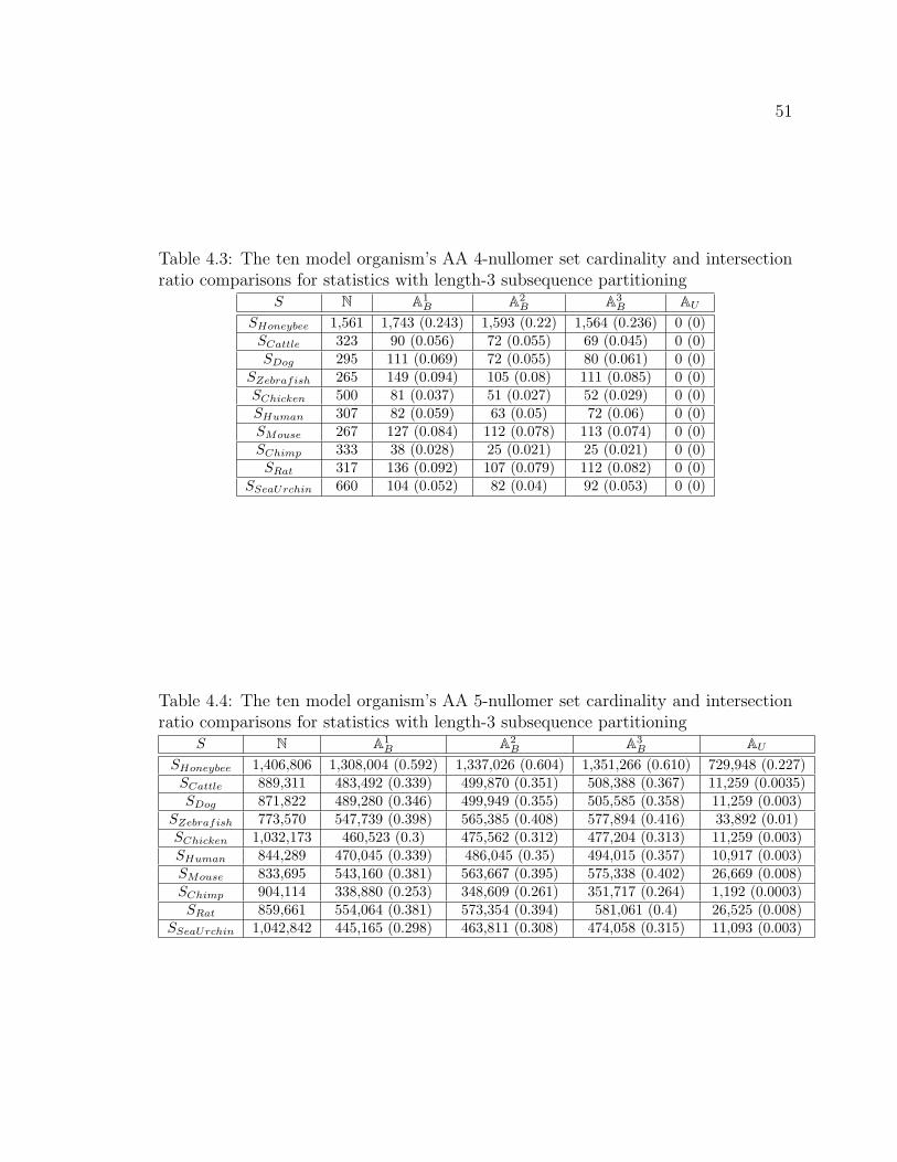
51

Table 4.3: The ten model organism’s AA 4-nullomer set cardinality and intersectionratio comparisons for statistics with length-3 subsequence partitioning

S N A1B A2

B A3B AU

SHoneybee 1,561 1,743 (0.243) 1,593 (0.22) 1,564 (0.236) 0 (0)SCattle 323 90 (0.056) 72 (0.055) 69 (0.045) 0 (0)SDog 295 111 (0.069) 72 (0.055) 80 (0.061) 0 (0)

SZebrafish 265 149 (0.094) 105 (0.08) 111 (0.085) 0 (0)SChicken 500 81 (0.037) 51 (0.027) 52 (0.029) 0 (0)SHuman 307 82 (0.059) 63 (0.05) 72 (0.06) 0 (0)SMouse 267 127 (0.084) 112 (0.078) 113 (0.074) 0 (0)SChimp 333 38 (0.028) 25 (0.021) 25 (0.021) 0 (0)SRat 317 136 (0.092) 107 (0.079) 112 (0.082) 0 (0)

SSeaUrchin 660 104 (0.052) 82 (0.04) 92 (0.053) 0 (0)

Table 4.4: The ten model organism’s AA 5-nullomer set cardinality and intersectionratio comparisons for statistics with length-3 subsequence partitioning

S N A1B A2

B A3B AU

SHoneybee 1,406,806 1,308,004 (0.592) 1,337,026 (0.604) 1,351,266 (0.610) 729,948 (0.227)SCattle 889,311 483,492 (0.339) 499,870 (0.351) 508,388 (0.367) 11,259 (0.0035)SDog 871,822 489,280 (0.346) 499,949 (0.355) 505,585 (0.358) 11,259 (0.003)

SZebrafish 773,570 547,739 (0.398) 565,385 (0.408) 577,894 (0.416) 33,892 (0.01)SChicken 1,032,173 460,523 (0.3) 475,562 (0.312) 477,204 (0.313) 11,259 (0.003)SHuman 844,289 470,045 (0.339) 486,045 (0.35) 494,015 (0.357) 10,917 (0.003)SMouse 833,695 543,160 (0.381) 563,667 (0.395) 575,338 (0.402) 26,669 (0.008)SChimp 904,114 338,880 (0.253) 348,609 (0.261) 351,717 (0.264) 1,192 (0.0003)SRat 859,661 554,064 (0.381) 573,354 (0.394) 581,061 (0.4) 26,525 (0.008)

SSeaUrchin 1,042,842 445,165 (0.298) 463,811 (0.308) 474,058 (0.315) 11,093 (0.003)

52

Table 4.5: The ten model organism’s AA 5-nullomer ranking histogram chi-squarecomparisons for statistics with length-3 subsequence partitioning

S Histogram N A1B A2

B A3B AU

SHoneybee H[0QSHoneybee

5,1 ] 0.1894 0.2127 0.2083 0.2032 0.98SHoneybee H[0QSHoneybee

5,2 ] 0.1997 0.2128 0.2183 0.2113 0.9317SHoneybee H[0QSHoneybee

5,3 ] 0.2055 0.2143 0.2199 0.2205 0.5082SCattle H[0QSCattle



5,3 ] 0.3147 0.4898 0.4892 0.4904 0.7570SDog H[0QSDog

5,1 ] 0.1613 0.2837 0.2674 0.2543 0.9796SDog H[0QSDog

5,2 ] 0.1720 0.2838 0.2789 0.2627 0.6842SDog H[0QSDog

5,3 ] 0.1755 0.2851 0.2802 0.2801 0.4781SZebrafish H[0QSZebrafish



5,3 ] 0.2290 0.2944 0.2949 0.2967 0.5161SChicken H[0QSChicken



5,3 ] 0.1712 0.3129 0.3108 0.3081 0.5528SHuman H[0QSHuman

5,1 ] 0.2646 0.4431 0.4180 0.3972 0.98SHuman H[0QSHuman

5,2 ] 0.2829 0.4436 0.4433 0.4159 0.98SHuman H[0QSHuman

5,3 ] 0.2911 0.4456 0.4453 0.4452 0.8722SMouse H[0QSMouse

5,1 ] 0.2605 0.3887 0.3686 0.3502 0.98SMouse H[0QSMouse

5,2 ] 0.2788 0.3890 0.3913 0.3680 0.9799SMouse H[0QSMouse

5,3 ] 0.2872 0.3909 0.3932 0.3955 0.8131SChimp H[0QSChimp

5,1 ] 0.1874 0.4256 0.4013 0.3819 0.98SChimp H[0QSChimp

5,2 ] 0.2010 0.4255 0.4210 0.3970 0.98SChimp H[0QSChimp

5,3 ] 0.2055 0.4274 0.4229 0.4219 0.9249SRat H[0QSRat

5,1 ] 0.1673 0.2574 0.2426 0.2316 0.98SRat H[0QSRat

5,2 ] 0.1799 0.2575 0.2575 0.2432 0.9799SRat H[0QSRat

5,3 ] 0.1843 0.2588 0.2588 0.2586 0.7196SSeaUrchin H[0QSSeaUrchin



5,3 ] 0.1789 0.3393 0.3428 0.3434 0.8002

53

Table 4.6: The ten model organism’s 3-FS, 4-FS, and 5-FS histogram chi-squarecomparisons for the [0, 10000] frequency spectral-range

S Histogram N A1B A2

B A3B AU

SHoneybee ΓSHoneybee

3 0.0038 0.0026 0.0035 0.0036 0.2058SHoneybee ΓSHoneybee

4 0.3084 0.2905 0.2988 0.3041 0.8571SHoneybee ΓSHoneybee

5 0.9761 0.9797 0.9792 0.9780 0.98SCattle ΓSCattle



5 0.8321 0.8693 0.8628 0.8624 0.9800SDog ΓSDog

3 0.0078 0.0028 0.0030 0.003 0.02SDog ΓSDog

4 0.0274 0.0691 0.0727 0.0744 0.4579SDog ΓSDog

5 0.5643 0.8690 0.8633 0.864 0.98SZebrafish ΓSZebrafish



5 0.8927 0.9231 0.9145 0.9099 0.98SChicken ΓSChicken



5 0.9490 0.8754 0.8686 0.8686 0.98SHuman ΓSHuman

3 0.0038 0.0032 0.0033 0.0033 0.02SHuman ΓSHuman

4 0.0753 0.0690 0.0725 0.0744 0.4533SHuman ΓSHuman

5 0.8307 0.8704 0.8642 0.8635 0.98SMouse ΓSMouse

3 0.0029 0.0027 0.0027 0.0027 0.02SMouse ΓSMouse

4 0.0916 0.0842 0.0878 0.0898 0.4667SMouse ΓSMouse

5 0.8728 0.9072 0.8986 0.8953 0.98SChimp ΓSChimp

3 0.0050 0.0045 0.0046 0.0044 0.02SChimp ΓSChimp

4 0.0489 0.0448 0.0476 0.0489 0.3822SChimp ΓSChimp

5 0.7071 0.7815 0.7820 0.7863 0.9796SRat ΓSRat

3 0.0031 0.0026 0.0027 0.0027 0.02SRat ΓSRat

4 0.0921 0.0847 0.0886 0.0905 0.4654SRat ΓSRat

5 0.8715 0.9046 0.8960 0.8938 0.98SSeaUrchin ΓSSeaUrchin



5 0.8226 0.8837 0.8752 0.8718 0.98

54

Table 4.7: The analysis summary of the ten model organism 3-FS distributions inFigures 4.1, 4.2, 4.3, 4.4, and 4.5

S/Rτ Standard Deviation Skewness KurtosisSHoneybee 0.0136 3.223 9.856SCattle 0.006 1.302 0.410SDog 0.003 0.407 -1.119

SZebrafish 0.007 0.792 0.792SChicken 0.009 2.278 0.041SHuman 0.006 1.293 0.421SMouse 0.007 1.469 0.920SChimp 0.005 0.859 -0.623SRat 0.007 1.507 1.072

SSeaUrchin 0.006 1.093 -0.073

Figure 4.1: Apis mellifera vs. Bos taurus: The ΓSHoneybee3 and ΓSCattle3 comparison with

a frequency spectral-range [0, 10000] for N data sets (only [0, 200] is shown)

55

Figure 4.2: Canis familiaris vs. Gallus gallus: The ΓSDog3 and ΓSChicken3 comparison

with a frequency spectral-range [0, 10000] for the N data sets (only [0, 200] is shown)

Figure 4.3: Danio rerio vs. Stronglyocentrus purpuratus: The ΓSZebrafish3 and

ΓSSeaUrchin3 comparison with a frequency spectral-range [0, 10000] for the N data sets(only [0, 200] is shown)

56

Figure 4.4: Homo sapien vs. Pan troglodytes: The ΓSHuman3 and ΓSChimp3 comparison


Figure 4.5: Mus musculus vs. Rattus norvegicus: The ΓSMouse3 and ΓSRat3 comparison


57

4.3.3 Bacteria Strain Results: Escherichia coli

This sections reports the DNA nullomer and 5-FS histogram results obtained from

conducting this experiment on two distinct strains and three distinct regions of the

EC bacteria.

Tables 4.8 and 4.9 display the experimental parameters. In Table 4.9, we see that

the EC-55989 genome is the longest, and that in both strains, the non-coding region

is longer than the coding region.

Tables 4.10 and 4.11, respectively, display the 8-nullomer set cardinality and

intersection ratio statistics for comparison between the three data set categories.

There are seven lengths for the AB data sets. For both strains and for all three

regions, the N 8-nullomer set cardinalities are greater than those of all the AB and

AU , except for the A7B. Moreover, both strains and all three regions, the AU 8-nullomer

set cardinalities and intersection ratios are zero. Furthermore, for both strains, the N

8-nullomer set cardinalities are the smallest for the complete region and the largest for

the non-coding region. So for both strains and all three regions, the AB 8-nullomer set

cardinalities and intersection ratios monotonically increase with the partition length.

To summarize, this suggests that in general, the N sequences are non-random because

their 8-nullomer set statistics strongly deviate from the AU sequences. Furthermore,

the AB sequences appear less random as the partition length increases.




regions, the N 9-nullomer set cardinalities are greater than those of all the AB

and AU , except for the A7B of the coding and non-coding regions for both strains.

58

Moreover, for both strains, with the complete and coding regions, the AU 9-nullomer

set cardinalities and intersection ratios are zero. Furthermore, for both strains, the N

9-nullomer set cardinalities are the smallest for the complete region and the largest for

the non-coding region. So for both strains and all three regions, the AB 9-nullomer set

cardinalities and intersection ratios monotonically increase with the partition length.

To summarize, this suggests that in general, the N sequences are non-random because

their 9-nullomer set statistics strongly deviate from the AU sequences. Furthermore,

the AB sequences appear less random as the partition length increases.




regions, the N 10-nullomer set cardinalities are greater than those of all the artificially-

generated. Moreover, both strains and for all three regions, the randomly-unbiased 10-

nullomer set cardinalities are less than those of the N and AB. Furthermore, for both

strains, with the complete and coding regions, the AU 10-nullomer set intersection

ratios are zero. Additionally, for both strains, the N 10-nullomer set cardinalities

are the smallest for the complete region and the largest for the non-coding region.

Finally, for both strains and all three regions, the AB 10-nullomer set cardinalities and

intersection ratios monotonically increase with the partition length. To summarize,

this suggests that in general, the N sequences are non-random because they strongly

deviate from the AU sequences. Furthermore, the AB sequences appear less random

as the partition length increases.

Table 4.16 displays the chi-square’s for Rankseq’s 10-nullomer probability his-

tograms. For both strains, for all three regions, and for all histogram lengths, the

randomly-unbiased chi-squares are the greatest. Moreover, based on these results, it

59

is possible to use the chi-square values for the N and AB data sets, for both strains, for

all histogram lengths, to delineate the coding region from the non-coding region: the

coding region chi-square range is [0.277, 0.8931] and the non-coding region chi-square

range is [0.926, 0.9899]. To summarize, the non-coding region chi-squares for the

N and AB data set 10-nullomer statistics are similar to the AU chi-squares, which

indicate that the non-coding regions are more random than the coding regions.

Figures 4.6 and 4.7 are depictions of the 5-FS histogram results, which compare the

complete (unfiltered), coding-region (filtered), and non-coding region (filtered) N data

sets. In Table 4.17, we see an analysis summary of these distributions. Interestingly,

the complete and coding regions of both strains are remarkably similar in terms

of standard deviation and skew, but the kurtosis of the complete regions is clearly

distinct (5.167 versus -0.894). Moreover, all regions for both strains exhibit a positive

skew, with the non-coding regions exhibiting the largest skew by one magnitude order.

In general, the coding and non-coding regions for both strains are clearly distinct from

each other.

Table 4.8: The EC bacteria’s DNA k-FS analysis configurationVariable Value Affected Programncbi filter NULL/CDS/Non-CDS Cseq

sequence type DNA Cseqsequence length 10 Cseq





The conclusions of this experiment are recapitulated in Section 5.1.

60

Table 4.9: The EC bacteria’s DNA sequence data sets. Here, the superregion length|Rτ | is used as Genseq’s “generation size”

S/Rτ Region Type |Rτ |SEC−536/RALL Complete 4,938,920SEC−536/RCDS Coding 4,324,150SEC−536/R¬CDS Non-Coding 614,770SEC−5598/RALL Complete 5,158,462SEC−5598/RCDS Coding 4,466,129SEC−5598/R¬CDS Non-Coding 688,733

Table 4.10: The EC bacteria’s DNA 8-nullomer set cardinality comparisons forstatistics with length-7 subsequence partitioning

S/Rτ N A1B A2

B A3B A4

B A5B A6

B A7B AU

SEC−536/RALL 32 0 0 0 17 21 25 45 0SEC−536/RCDS 75 0 0 0 50 64 79 133 0SEC−536/R¬CDS 488 4 3 29 211 278 374 660 0SEC−5598/RALL 31 0 0 0 17 24 22 35 0SEC−5598/RCDS 95 0 0 0 51 58 74 121 0SEC−5598/R¬CDS 425 2 1 19 179 271 347 611 0

Table 4.11: The EC bacteria’s DNA 8-nullomer set intersection ratio comparisons forstatistics with length-7 subsequence partitioning

S/Rτ A1B A2

B A3B A4

B A5B A6

B A7B AU

SEC−536/RALL 0.0 0.0 0.0 0.089 0.120 0.130 0.329 0.0SEC−536/RCDS 0.0 0.0 0.0 0.134 0.177 0.261 0.543 0.0SEC−536/R¬CDS 0.0 0.0 0.012 0.140 0.179 0.223 0.468 0.0SEC−5598/RALL 0.0 0.0 0.0 0.030 0.079 0.085 0.154 0.0SEC−5598/RCDS 0.0 0.0 0.0 0.123 0.147 0.157 0.335 0.0SEC−5598/R¬CDS 0.0 0.0 0.010 0.131 0.213 0.256 0.485 0.0


S/Rτ N A1B A2

B A3B A4

B A5B A6

B A7B AU

SEC−536/RALL 1,894 0 0 115 1,477 1,619 1,736 1,965 0SEC−536/RCDS 3,054 0 1 293 2,303 2,596 2,899 3,324 0SEC−536/R¬CDS 28,346 7,450 9,602 13,512 17,978 19,842 22,267 26,597 2,422SEC−5598/RALL 1,920 0 0 103 1,408 1,576 1,692 1,927 0SEC−5598/RCDS 3,322 0 1 298 2,281 2,591 2,850 3,439 0SEC−5598/R¬CDS 24,248 5,214 6,901 10,340 14,682 16,401 18,475 22,245 1,389

61

Table 4.13: The EC bacteria’s DNA 9-nullomer set intersection ratio comparisons forstatistics with length-7 subsequence partitioning

S/Rτ A1B A2

B A3B A4

B A5B A6

B A7B AU



S/Rτ N A1B A2

B A3B A4

B A5B A6

B A7B AU

SEC−536/RALL 59,585 99 4,041 23,158 41,817 47,801 52,802 56,405 95SEC−536/RCDS 83,054 382 8,123 36,266 58,691 68,063 74,765 79,818 288SEC−536/R¬CDS 491,039 362,906 387,142 406,369 421,972 429,537 439,834 456,539 324,804SEC−5598/RALL 57,934 71 3,416 21,557 39,443 45,370 50,413 54,033 62SEC−5598/RCDS 83,510 341 7,462 35,465 57,289 66,791 73,528 79,285 221SEC−5598/R¬CDS 459,321 322,325 348,710 368,540 385,692 392,911 402,475 418,988 282,149

Table 4.15: The EC bacteria’s DNA 10-nullomer set intersection ratio comparisonsfor statistics with length-7 subsequence partitioning

S/Rτ A1B A2

B A3B A4

B A5B A6

B A7B AU


62

Table 4.16: The EC bacteria’s DNA 10-nullomer ranking histogram chi-square com-parisons for statistics with length-7 subsequence partitioning

S/Rτ Histogram N A1B A2

B A3B A4

B A5B A6

B A7B AU

SEC−536/RALL H[0QRALL

10,1 ] 0.8733 0.9070 0.9323 0.9035 0.9079 0.9007 0.8892 0.9068 0.98


10,2 ] 0.2080 0.9051 0.2861 0.2580 0.2364 0.2250 0.2124 0.2109 0.98


10,3 ] 0.2044 0.8999 0.2861 0.2864 0.2488 0.2271 0.2125 0.2103 0.98


10,4 ] 0.2553 0.8825 0.2862 0.2865 0.3250 0.2939 0.2718 0.2634 0.9789


10,5 ] 0.2950 0.8372 0.2857 0.2870 0.3257 0.3461 0.3177 0.3064 0.9230


10,6 ] 0.3308 0.7378 0.2851 0.2886 0.3284 0.3489 0.3666 0.3497 0.7827


10,7 ] 0.3580 0.5089 0.2850 0.2939 0.3381 0.3594 0.3774 0.392 0.5353

SEC−536/RCDS H[0QRCDS

10,1 ] 0.7065 0.8652 0.7974 0.7259 0.7391 0.7354 0.7226 0.7664 0.98


10,2 ] 0.3968 0.8685 0.5510 0.4710 0.4400 0.4201 0.4051 0.4003 0.98


10,3 ] 0.5730 0.8755 0.5512 0.7790 0.6920 0.6400 0.6008 0.5889 0.98


10,4 ] 0.6877 0.8844 0.5518 0.7793 0.8279 0.7715 0.7279 0.709 0.98


10,5 ] 0.7595 0.8931 0.5532 0.7805 0.8286 0.8538 0.8076 0.7862 0.98


10,6 ] 0.8100 0.8970 0.5591 0.7842 0.8314 0.8563 0.8653 0.8415 0.9748


10,7 ] 0.8411 0.8789 0.5782 0.7960 0.8405 0.8636 0.8726 0.8799 0.9284

SEC−536/R¬CDS H[0QR¬CDS

10,1 ] 0.9799 0.9795 0.9797 0.9799 0.9799 0.9799 0.9799 0.9778 0.98


10,2 ] 0.9705 0.9795 0.9725 0.9725 0.9718 0.9710 0.9704 0.9689 0.98


10,3 ] 0.9676 0.9795 0.9725 0.9705 0.9697 0.9690 0.9684 0.9671 0.98


10,4 ] 0.9668 0.9794 0.9725 0.9705 0.9695 0.9689 0.9683 0.9668 0.98


10,5 ] 0.9653 0.9789 0.9724 0.9705 0.9695 0.9684 0.9676 0.9658 0.98


10,6 ] 0.9632 0.9784 0.9722 0.9704 0.9694 0.9683 0.9675 0.9654 0.98


10,7 ] 0.9606 0.9772 0.9715 0.9700 0.9690 0.9681 0.9674 0.9652 0.9799


10,1 ] 0.9745 0.9450 0.9686 0.9746 0.9748 0.9734 0.9721 0.9778 0.98


10,2 ] 0.2237 0.9441 0.3112 0.2788 0.2551 0.2417 0.2288 0.2275 0.98


10,3 ] 0.2219 0.9385 0.3114 0.3134 0.2729 0.2489 0.2322 0.2287 0.98


10,4 ] 0.2806 0.9187 0.3113 0.3136 0.3618 0.3274 0.3014 0.2911 0.98


10,5 ] 0.3241 0.8576 0.3116 0.3141 0.3625 0.3853 0.3528 0.3390 0.9756


10,6 ] 0.3664 0.6807 0.3123 0.3161 0.3655 0.3884 0.4095 0.3895 0.8126


10,7 ] 0.3968 0.4601 0.3135 0.3231 0.3762 0.3997 0.4214 0.4375 0.4844


10,1 ] 0.4600 0.4616 0.4456 0.4150 0.4465 0.4483 0.4495 0.4626 0.98


10,2 ] 0.2710 0.4615 0.3987 0.3365 0.3130 0.2955 0.2809 0.2770 0.98


10,3 ] 0.2995 0.4611 0.3990 0.4369 0.3792 0.3440 0.3186 0.3110 0.98


10,4 ] 0.3869 0.4614 0.3992 0.4371 0.5103 0.4575 0.4222 0.4058 0.9799


10,5 ] 0.4611 0.4665 0.3991 0.4379 0.5115 0.5598 0.5120 0.4889 0.9750


10,6 ] 0.5168 0.4762 0.3964 0.4415 0.5153 0.5636 0.5859 0.5555 0.8171


10,7 ] 0.5586 0.4754 0.3860 0.4542 0.5288 0.5763 0.5980 0.6154 0.5143


10,1 ] 0.9750 0.9722 0.9741 0.9756 0.9753 0.9749 0.9742 0.9632 0.98


10,2 ] 0.9469 0.9721 0.9539 0.9519 0.9498 0.9482 0.9473 0.9449 0.98


10,3 ] 0.9448 0.9717 0.9538 0.9522 0.9498 0.9486 0.9473 0.9450 0.98


10,4 ] 0.9426 0.9708 0.9538 0.9522 0.9495 0.9486 0.9471 0.9443 0.98


10,5 ] 0.9405 0.9686 0.9536 0.9521 0.9493 0.9478 0.9459 0.9429 0.98


10,6 ] 0.9375 0.9659 0.9531 0.9519 0.9490 0.9476 0.9464 0.9426 0.9799


10,7 ] 0.9342 0.9612 0.9516 0.9510 0.9482 0.9471 0.9460 0.9434 0.9795

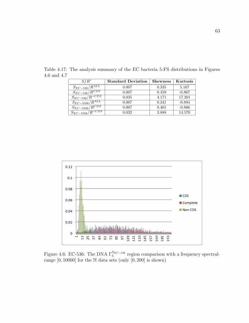
63

Table 4.17: The analysis summary of the EC bacteria 5-FS distributions in Figures4.6 and 4.7

S/Rτ Standard Deviation Skewness KurtosisSEC−536/RALL 0.007 0.335 5.167SEC−536/RCDS 0.007 0.459 -0.867SEC−536/R¬CDS 0.035 4.171 17.201SEC−5598/RALL 0.007 0.341 -0.894SEC−5598/RCDS 0.007 0.401 -0.866SEC−5598/R¬CDS 0.032 3.888 14.570

Figure 4.6: EC-536: The DNA ΓSEC−536

5 region comparison with a frequency spectral-range [0, 10000] for the N data sets (only [0, 200] is shown)

64

Figure 4.7: EC-55989: The DNA ΓSEC−55989

5 region comparison with a frequencyspectral-range [0, 10000] for the N data sets (only [0, 200] is shown)

65

4.3.4 Virus Strain Results: Human immunodeficiency virus

This sections reports the DNA/RNA nullomer results and the 3-FS results obtained

from conducting this experiment on two distinct strains and three distinct regions of

HIV.

Tables 4.18 and 4.19 display the experimental parameters. In Table 4.19, we see

that the HIV-2 genome is the longest, and that in both strains, the coding region is

longer than the non-coding region.

Table 4.20 displays the 5-nullomer set cardinality and intersection ratio statistics.

For both strains, we see that the complete region 5-nullomer set cardinality is the

smallest and that of the non-coding region is the greatest. Moreover, for both strains,

for all regions, the AU 5-nullomer set cardinalities and intersection ratios are the

smallest, where those for the complete and coding regions are zero. Furthermore,

for both strains, for all regions, the AB 5-nullomer set cardinalities and intersection

ratios monotonically increase as the partition length increases. Additionally, for both

strains, for the non-coding regions, the N 5-nullomer set cardinalities are greater

than those of the AB and AU . Likewise, for the HIV-1 strain, for complete and

coding regions, the 5-nullomer set cardinalities are greater than those of the A1B, and

less than those of the A2B and A3

B. Finally, for the HIV-2 strain, for complete and

coding regions, the 5-nullomer set cardinalities are greater than those of the A1B and

A2B, and less than those of the A3

B, with the exception of the complete region, which

is actually greater than the length-3 value.



smallest and the non-coding region is the greatest. Moreover, for both strains, for all

66

regions, the AU 6-nullomer set cardinalities and intersection ratios are the smallest.

Furthermore, for both strains, for all regions, the AB 6-nullomer set cardinalities and

intersection ratios monotonically increase as the partition length increases. Addition-

ally, for both strains, for the non-coding regions, the N 6-nullomer set cardinalities

are greater than those of the AB and AU . So for the complete and coding regions of

both strains, the N 6-nullomer set cardinalities are greater than those of the A1B and

less than those of the A2B and A3

B.



smallest and the non-coding region is the greatest. Moreover, for both strains, for all

regions, the AU 7-nullomer set cardinalities and intersection ratios are the smallest,

with the exception of the HIV-1 non-coding region, which is equivalent to that of the

A1B. Furthermore, for both strains, for all regions, the AB 7-nullomer set cardinalities

and intersection ratios monotonically increase as the partition length increases. So

for all three regions of both strains, we see that the N 7-nullomer set cardinalities are

greater than those of the AB and AU .

Table 4.23 displays the chi-squares for Rankseq’s 7-nullomer probability histograms.

For both strains, for all three regions, and for all histogram lengths, with the excep-

tion of the HIV-2 strain’s P (3) histogram for the non-coding region, the randomly-

unbiased chi-squares are the greatest. Moreover, based on these results, it is possible

to use the chi-square values for the N and AB data sets, for both strains, for all

histogram lengths, to delineate the coding region from the non-coding region: for the

HIV-1 strain, the coding region chi-square range is [0.1874, 0.2498] and the non-coding

region chi-square range is [0.6029, 0.8839], and likewise for the HIV-2 strain, the

coding region chi-square range is [0.1351, 0.1743] and the non-coding region chi-square

67

range is [0.4795, 0.5174]. Therefore, based on these chi-square ranges, it is possible

to distinguish between the two strains because the HIV-2 ranges are smaller and do

not overlap with the HIV-1 ranges. To summarize, the non-coding region 7-nullomer

statistics of the N and AB sequences are similar to those of the AU sequences: the

non-coding regions are more random than the coding regions.

Figures 4.8 and 4.9 display the 3-FS results for the N data sets. In Table 4.24,

we see an analysis summary of these distributions. Interestingly, the kurtosis of all

regions for both strains is negative, except for HIV-1’s non-coding region. Moreover,

all regions of both strains exhibit a positive skew. Furthermore, non-coding region

of HIV-1 has the greatest skew, and the non-coding region of HIV-2 has the smallest

skew. Similarly to the EC bacteria, the non-coding regions for both HIV strains are

clearly distinct from the coding regions.

Table 4.18: The HIV’s DNA/RNA k-FS analysis configurationVariable Value Affected Programncbi filter NULL/CDS/Non-CDS Cseq

sequence type DNA Cseqsequence length 7 Cseq






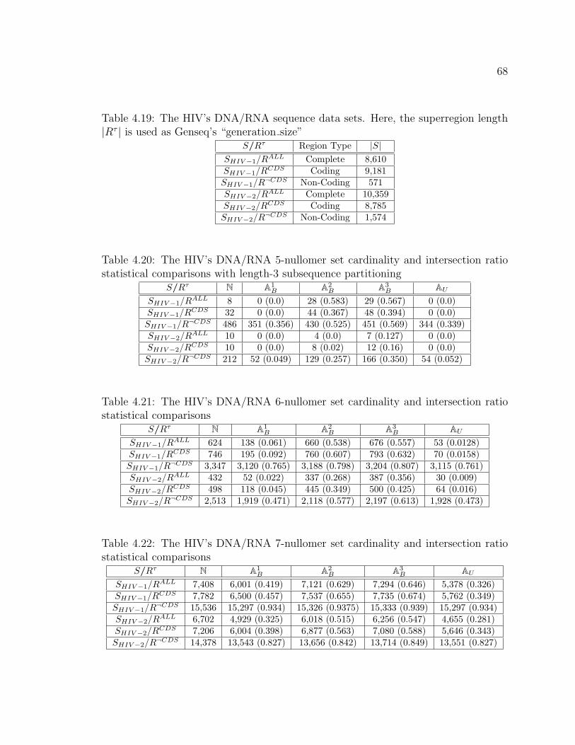
68

Table 4.19: The HIV’s DNA/RNA sequence data sets. Here, the superregion length|Rτ | is used as Genseq’s “generation size”

S/Rτ Region Type |S|SHIV−1/RALL Complete 8,610SHIV−1/RCDS Coding 9,181SHIV−1/R¬CDS Non-Coding 571SHIV−2/RALL Complete 10,359SHIV−2/RCDS Coding 8,785SHIV−2/R¬CDS Non-Coding 1,574

Table 4.20: The HIV’s DNA/RNA 5-nullomer set cardinality and intersection ratiostatistical comparisons with length-3 subsequence partitioning

S/Rτ N A1B A2

B A3B AU

SHIV−1/RALL 8 0 (0.0) 28 (0.583) 29 (0.567) 0 (0.0)SHIV−1/RCDS 32 0 (0.0) 44 (0.367) 48 (0.394) 0 (0.0)SHIV−1/R¬CDS 486 351 (0.356) 430 (0.525) 451 (0.569) 344 (0.339)SHIV−2/RALL 10 0 (0.0) 4 (0.0) 7 (0.127) 0 (0.0)SHIV−2/RCDS 10 0 (0.0) 8 (0.02) 12 (0.16) 0 (0.0)SHIV−2/R¬CDS 212 52 (0.049) 129 (0.257) 166 (0.350) 54 (0.052)

Table 4.21: The HIV’s DNA/RNA 6-nullomer set cardinality and intersection ratiostatistical comparisons

S/Rτ N A1B A2

B A3B AU

SHIV−1/RALL 624 138 (0.061) 660 (0.538) 676 (0.557) 53 (0.0128)SHIV−1/RCDS 746 195 (0.092) 760 (0.607) 793 (0.632) 70 (0.0158)SHIV−1/R¬CDS 3,347 3,120 (0.765) 3,188 (0.798) 3,204 (0.807) 3,115 (0.761)SHIV−2/RALL 432 52 (0.022) 337 (0.268) 387 (0.356) 30 (0.009)SHIV−2/RCDS 498 118 (0.045) 445 (0.349) 500 (0.425) 64 (0.016)SHIV−2/R¬CDS 2,513 1,919 (0.471) 2,118 (0.577) 2,197 (0.613) 1,928 (0.473)

Table 4.22: The HIV’s DNA/RNA 7-nullomer set cardinality and intersection ratiostatistical comparisons

S/Rτ N A1B A2

B A3B AU

SHIV−1/RALL 7,408 6,001 (0.419) 7,121 (0.629) 7,294 (0.646) 5,378 (0.326)SHIV−1/RCDS 7,782 6,500 (0.457) 7,537 (0.655) 7,735 (0.674) 5,762 (0.349)SHIV−1/R¬CDS 15,536 15,297 (0.934) 15,326 (0.9375) 15,333 (0.939) 15,297 (0.934)SHIV−2/RALL 6,702 4,929 (0.325) 6,018 (0.515) 6,256 (0.547) 4,655 (0.281)SHIV−2/RCDS 7,206 6,004 (0.398) 6,877 (0.563) 7,080 (0.588) 5,646 (0.343)SHIV−2/R¬CDS 14,378 13,543 (0.827) 13,656 (0.842) 13,714 (0.849) 13,551 (0.827)

69

Table 4.23: Rankseq’s HIV DNA/RNA 7-nullomer probability histogram chi-squarecomparisons with length-3 subsequence partitioning

S/Rτ Histogram N A1B A2

B A3B AU

SHIV−1/RALL H[0QRALL

7,1 ] 0.1837 0.1968 0.196 0.1922 0.9609SHIV−1/RALL H[0QR

ALL

7,2 ] 0.2199 0.1948 0.2334 0.2291 0.7963SHIV−1/RALL H[0QR

ALL

7,3 ] 0.2219 0.1896 0.2332 0.2341 0.4273SHIV−1/RCDS H[0QR

CDS

7,1 ] 0.1874 0.1988 0.1968 0.1929 0.9585SHIV−1/RCDS H[0QR

CDS

7,2 ] 0.2352 0.1932 0.2476 0.2443 0.7751SHIV−1/RCDS H[0QR

CDS

7,3 ] 0.2368 0.1873 0.2471 0.2498 0.4121SHIV−1/R¬CDS H[0QR

¬CDS

7,1 ] 0.8205 0.7799 0.8027 0.8839 0.9414SHIV−1/R¬CDS H[0QR

¬CDS

7,2 ] 0.6307 0.7170 0.6385 0.6438 0.7965SHIV−1/R¬CDS H[0QR

¬CDS

7,3 ] 0.6079 0.6423 0.6357 0.6198 0.6524SHIV−2/RALL H[0QR

ALL

7,1 ] 0.1360 0.1454 0.1430 0.1428 0.5778SHIV−2/RALL H[0QR

ALL

7,2 ] 0.1111 0.1451 0.1206 0.1169 0.4909SHIV−2/RALL H[0QR

ALL

7,3 ] 0.1167 0.1400 0.1220 0.1261 0.3345SHIV−2/RCDS H[0QR

CDS

7,1 ] 0.1743 0.1705 0.1660 0.1640 0.7609SHIV−2/RCDS H[0QR

CDS

7,2 ] 0.1351 0.1674 0.1419 0.1417 0.5264SHIV−2/RCDS H[0QR

CDS

7,3 ] 0.1451 0.1599 0.1446 0.1545 0.3508SHIV−2/R¬CDS H[0QR

¬CDS

7,1 ] 0.5174 0.4945 0.4978 0.4980 0.5535SHIV−2/R¬CDS H[0QR

¬CDS

7,2 ] 0.4795 0.4966 0.4928 0.4865 0.5044SHIV−2/R¬CDS H[0QR

¬CDS

7,3 ] 0.4894 0.4882 0.4982 0.5123 0.4944

Table 4.24: The analysis summary of the HIV 3-FS distributions in Figures 4.8 and4.9

S/Rτ Standard Deviation Skewness KurtosisSHIV−1/RALL 0.052 0.557 -0.938SHIV−16/RCDS 0.054 0.904 -0.141SHIV−1/R¬CDS 0.103 1.840 1.685SHIV−2/RALL 0.067 0.994 -0.222SHIV−2/RCDS 0.052 0.520 -1.099SHIV−2/R¬CDS 0.059 0.894 -0.617

70

Figure 4.8: HIV-1: The DNA/RNA ΓSHIV−1

3 region comparison with a frequencyspectral-range [0, 300] for the N data set (only [0, 20] is shown)

Figure 4.9: HIV-2: The DNA/RNA ΓSHIV−2

3 region comparison with a frequencyspectral-range [0, 300] for the N data set (only [0, 20] is shown)

71

4.4 Experiment 2: NCBI Genome Database Evolution and

Time Series Analysis: Prime Prediction Assessment

4.4.1 Objective Summary

This experiment employs an ANN to investigate the prime phenomena by assessing

the chronological predictability within the growing NCBI database for DNA. This

supervised machine learning approach aims to capture the evolutionary behavior of

the NCBI database as the prime set cardinality monotonically decreases over time.

This investigation attempts to forecast the Boolean observed state for primes by

extracting the corresponding sequence traits and compiling them into feature vectors.

This experiment seeks answers to the following inquiries:

1. Is it feasible to forecast the Boolean observed prime states as the NCBI database

evolves and grows using an ANN?

2. Can our software analysis suite make a legitimate scientific assessment of this

phenomena?

4.4.2 Training, Testing, and Prediction Results: The Artificial Neural

Network

The objective is to assess the predictability of DNA 16-primes as the NCBI database

evolves over this 18-month period. In this case, we use Rankseq length-8 partitioning

statistics to compile feature vector examples from the chronologically ordered DNA

data sets from the contiguous NCBI database snapshots for training, testing, and

prediction.

72

Data Sets

For each monthly NCBI snapshot, we use Tdataformat to create both a balanced and

an unbalanced data set. The balanced series is equivalent to the unbalanced series

except that in the balanced data sets, minority oversampling is used to compile an

equal number of positive and negative examples in the data sets. Tables 4.25 and

4.26 display the chronologically ordered monthly NCBI database snapshot datasets

for the DNA 16-primes with length-8 subsequence partitioning statistics used to train

the ANN via supervised learning. Each training example of the 16-prime data sets

contains 14-element feature vectors, which correspond to 14 Rankseq attributes, where

the first 8 attributes are the prime probabilities for the partition length 1 ≤ ρ ≤ 8 in

the form

vρ = 0QSA,B16,ρ . (4.34)

So additionally, for an arbitrary monthly NCBI database snapshot SA,B, ∀s ∈ 0BSA,B16 ,

we have

v9 =F (g, s) + F (c, s)

F (a, s) + F (t, s) + F (c, s) + F (g, s), (4.35)

v10 =F (a, s) + F (t, s)

F (g, s) + F (c, s), (4.36)

v11 =F (cp, s)

F (c, s)× F (g, s)× |s|, (4.37)

v12 =F (a, s) + F (g, s)

|s|, (4.38)

v13 =F (c, s) + F (t, s)

|s|, (4.39)

v14 =F (a, s) + F (t, s)

|s|, (4.40)

73

for the GC-content, GC-ratio, CpG supression ratio, purine density, pyrimidine den-

sity, and AT-density, respectively, where 0BSA,B16 is the prime set using the formal

notation of Section 4.2.

We define SA and SB as the DNA sequence snapshots for months A and B,

respectively. Moreover, we define 0BSA16 and 0BSB

16 as the 16-prime sets for A and B,

respectively. Furthermore, we define 0BSA,B16 and 1B

SA,B16 as the negative and positive

training example sets for the snapshot SA,B, respectively, such that

0BSA,B16 = 0BSA

16 ∩ 0BSB16 , (4.41)

1BSA,B16 = 0BSB

16 − 0BSA16 . (4.42)

Table 4.25: The size statistics for the balanced NCBI data set snapshotsMonth Range SA,B Size (MB) # Total Examples

2010.01 to 2010.02 S1,2 1,100 8,245,6122010.02 to 2010.03 S2,3 972 7,776,4482010.03 to 2010.04 S3,4 953 7,624,3362010.04 to 2010.05 S4,5 926 7,406,3582010.05 to 2010.06 S5,6 879 7,031,3662010.06 to 2010.07 S6,7 818 6,544,8382010.07 to 2010.08 S7,8 791 6,326,7782010.08 to 2010.09 S8,9 780 6,242,4322010.09 to 2010.10 S9,10 684 5,471,3182010.10 to 2010.11 S10,11 659 5,270,7782010.11 to 2010.12 S11,12 649 5,191,3862010.12 to 2011.01 S12,13 589 4,711,6602011.01 to 2011.03 S13,14 470 3,754,5902011.03 to 2011.04 S14,15 463 3,701,6682011.04 to 2011.05 S15,16 443 3,542,6222011.05 to 2011.06 S16,17 426 3,407,2042011.06 to 2011.07 S17,18 401 3,205,760

So we define ϕ− as the ratio of negative training examples, which is identical to

the ratio of prime → prime transitions, and we define ϕ+ as the ratio of positive

74

Table 4.26: The size statistics for the unbalanced NCBI data set snapshotsMonth Range SA,B Size (MB) # Total Examples |1BS16| |0BS16|

2010.01 to 2010.02 S1,2 576 4,605,784 482,978 4,122,8062010.02 to 2010.03 S2,3 516 4,123,878 235,654 3,888,2242010.03 to 2010.04 S3,4 478 3,890,482 78,314 3,812,1682010.04 to 2010.05 S4,5 477 3,812,284 109,105 3,703,1792010.05 to 2010.06 S5,6 464 3,706,729 191,046 3,515,6832010.06 to 2010.07 S6,7 440 3,515,937 243,518 3,272,4192010.07 to 2010.08 S7,8 410 3,274,347 110,958 3,163,3892010.08 to 2010.09 S8,9 396 3,163,429 42,213 3,121,2162010.09 to 2010.10 S9,10 391 3,122,114 386,455 2,735,6592010.10 to 2010.11 S10,11 344 2,751,170 115,781 2,635,3892010.11 to 2010.12 S11,12 330 2,636,007 40,314 2,595,6932010.12 to 2011.01 S12,13 325 2,595,701 239,871 2,355,8302011.01 to 2011.03 S13,14 295 2,358,580 481,285 1,877,2952011.03 to 2011.04 S14,15 236 1,884,839 34,005 1,850,8342011.04 to 2011.05 S15,16 232 1,854,416 83,105 1,771,3112011.05 to 2011.06 S16,17 222 1,776,063 72,461 1,703,6022011.06 to 2011.07 S17,18 219 1,747,427 144,547 1,602,880

training examples, which is identical to the ratio of prime → oligomer transitions.

Therefore, we define

prime → prime : ϕSA,B− =

|0BSA,B16 |

|0BSA,B16 |+ |1BSA,B

16 |, (4.43)

prime → oligomer : ϕSA,B+ =

|1BSA,B16 |

|0BSA,B16 |+ |1BSA,B

16 |, (4.44)

as the ratio of negative and positive training examples for the NCBI snapshot SA,B,

respectively, such that ϕSA,B− + ϕ

SA,B+ = 1, where |0BSA,B

16 | + |1BSA,B16 | is the total

number of examples. Next, we define α− and α+ as Predictseq’s prediction default

accuracies for the negative and positive examples, respectively. Thus, in terms of

specific snapshots, we define αSA,B− and α

SA,B+ as Predictseq’s negative and positive

example default accuracies for the NCBI snapshot SA,B: so 0BSA,B16 is to α

SA,B− just as

1BSA,B16 is to α

SA,B+ . Therefore, we use

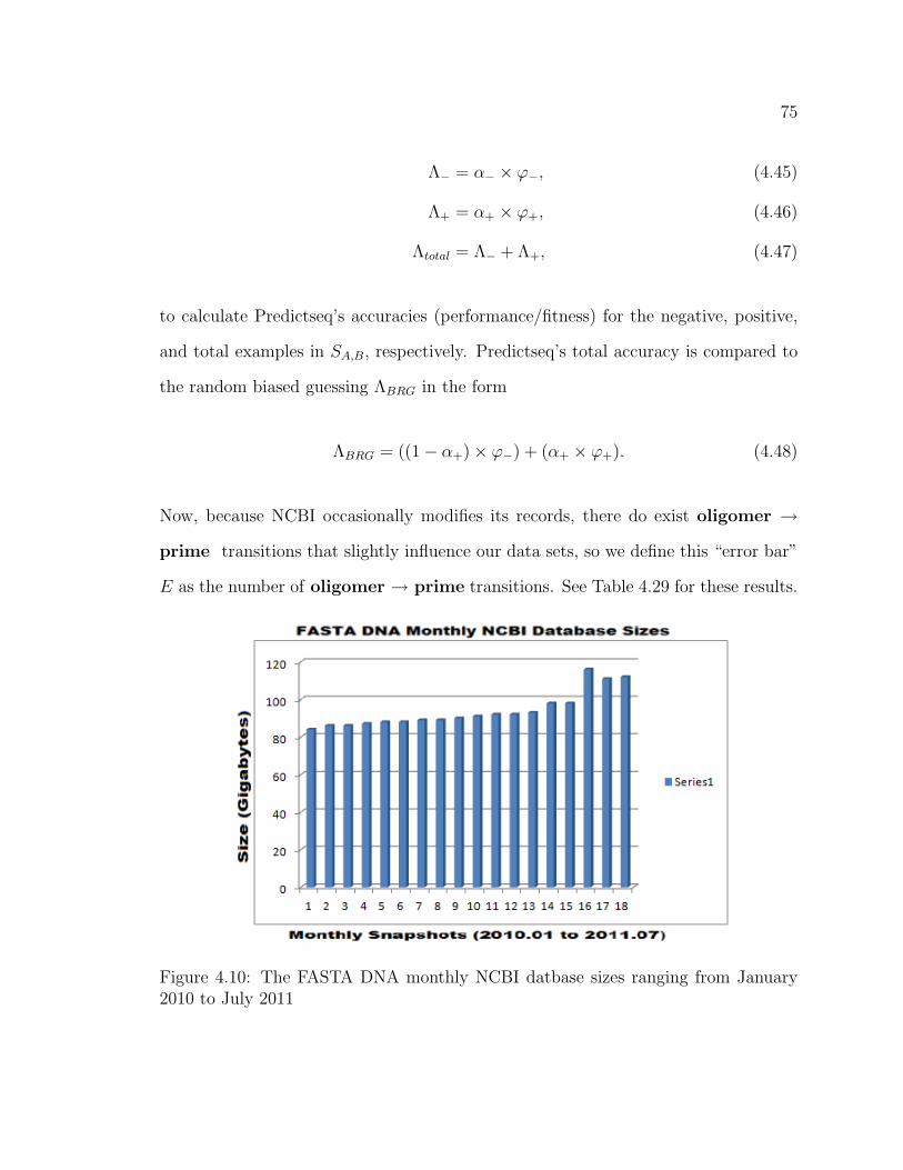
75

Λ− = α− × ϕ−, (4.45)

Λ+ = α+ × ϕ+, (4.46)

Λtotal = Λ− + Λ+, (4.47)

to calculate Predictseq’s accuracies (performance/fitness) for the negative, positive,

and total examples in SA,B, respectively. Predictseq’s total accuracy is compared to

the random biased guessing ΛBRG in the form

ΛBRG = ((1− α+)× ϕ−) + (α+ × ϕ+). (4.48)

Now, because NCBI occasionally modifies its records, there do exist oligomer →

prime transitions that slightly influence our data sets, so we define this “error bar”

E as the number of oligomer → prime transitions. See Table 4.29 for these results.

Figure 4.10: The FASTA DNA monthly NCBI datbase sizes ranging from January2010 to July 2011

76

Figure 4.11: The DNA 16-prime set cardinalities for the NCBI database snapshotsranging from January 2010 to July 2011

Note: Although this experiment was systematically conducted over an 18-month

period, the February 2011 NCBI snapshot was incomplete and thereby merged into

the subsequent month—giving us a total of 17 data sets.

Results: ANN Training and Testing Accuracy Evaluations

In this section, we report the ANN configuration, training, and testing results of the

NCBI data sets for (Boolean-valued) observed prime state prediction.

Table 4.27 displays the ANN architecture and training configuration for the Quick-

prop (Q), Incremental Quickprop (IQ), and Resilent Backprop (RB) algorithms. Table

4.28 displays the supervised learning training accuracies and fitness for the ANN on

the (balanced) chronologically ordered monthly database snapshots—the most fit

ANN state between the three training algorithms is bold highlighted and selected for

the testing phase.

77

Figure 4.12: The DNA 16-prime set sizes (in megabytes) for the NCBI ANN trainingand testing data sets ranging from January 2010 to July 2011


78

Table 4.27: The ANN training configuration for the observed prime state predictionson the monthly NCBI database snapshots

Parameter ValueLearning Rate: 0.5

Learning Momentum: 0.5Input (Layer) Size: 14

Hidden (Layer) Size: 4Output (Layer) Size: 1Activation Function: Sigmoid

Epochs: 40,000Target Accuracy: 90 %

Table 4.28: The ANN training accuracies for 16-prime state prediction on the balancedmonthly DNA data sets ranging from January 2010 to July 2011

SA,B Q (%) IQ (%) RB (%)S1,2 75.0 74.8 75.2S2,3 75.0 74.8 75.1S3,4 75.0 74.8 75.0S4,5 75.0 74.8 75.4S5,6 75.0 74.8 75.5S6,7 74.9 74.8 74.9S7,8 75.0 74.8 75.1S8,9 75.0 74.8 75.1S9,10 75.0 74.7 75.7S10,11 75.1 74.7 75.2S11,12 75.0 74.7 75.1S12,13 75.4 74.7 75.5S13,14 74.9 74.6 75.3S14,15 75.2 74.6 75.3S15,16 75.0 74.6 75.3S16,17 75.0 74.7 75.1S17,18 75.1 74.7 75.1

79

Table 4.29: Predictseq’s ANN prediction accuracies for the 16-prime state unbalancedmonthly DNA data sets ranging from February 2010 to July 2011. We see thatPredictseq’s accuracy Λtotal outperformed the random biased guessing ΛBRG in 14

16

cases.SA,B ϕ− % (|0BS16|) α− % Λ− % ϕ+ % (|1BS16|) α+ % Λtotal % ΛBRG % E #S1,2 89.54 (4,122,806) n/a n/a 10.46 (482,978) n/a n/a n/a 1,072S2,3 94.35 (3,888,224) 63.82 60.21 5.65 (235,654) 36.44 62.27 62.02 2,258S3,4 97.99 (3,812,168) 63.19 61.92 2.01 (78,314) 40.64 62.73 58.98 116S4,5 97.24 (3,703,179) 77.46 75.32 2.76 (109,105) 28.57 76.11 70.25 3,550S5,6 94.86 (3,515,683) 61.3 58.15 5.14 (191,046) 46.53 60.54 53.11 254S6,7 93.13 (3,272,419) 56.37 52.50 6.87 (243,518) 45.86 55.64 53.57 1,928S7,8 96.62 (3,163,389) 65.65 63.43 3.38 (110,958) 39.05 64.75 60.21 40S8,9 98.69 (3,121,216) 55 54.28 1.31 (42,213) 46.25 54.88 53.65 898S9,10 88.12 (2,735,659) 76.76 67.64 11.88 (386,455) 29.51 71.14 65.62 15,511S10,11 95.81 (2,635,389) 64.24 61.55 4.19 (115,781) 41.65 63.29 57.65 618S11,12 98.47 (2,595,693) 57.54 56.66 1.53 (40,314) 45.53 57.35 54.33 8S12,13 90.86 (2,355,830) 55.52 50.45 9.14 (239,871) 43.47 54.41 55.34 2,750S13,14 79.9 (1,877,295) 49.69 39.70 20.1 (481,285) 53.04 50.36 48.18 7,544S14,15 98.39 (1,850,834) 56.09 55.19 1.61 (34,005) 43.98 55.89 55.83 3,582S15,16 95.78 (1,771,311) 61.71 59.11 4.22 (83,105) 38.1 60.71 60.90 4,752S16,17 98.39 (1,703,602) 61.58 60.59 1.61 (72,461) 41.2 61.25 58.52 43,825S17,18 91.75 (1,602,880) 50.14 46.00 8.25 (144,547) 57.18 50.72 44.01 364

Figure 4.13: A depiction of the ANN 16-prime state prediction accuracies for the(unbalanced) monthly DNA data sets ranging from February 2010 to July 2011

80

CHAPTER 5

CONCLUSION

5.1 Results Discussion

In this section, we recapitulate the experimental results of Sections 4.3 and 4.4,

respectively.

5.1.1 Experiment 1

Nullomers: Absent k-mer Statistics

In the ten model organisms, based on the AA nullomer probability, ranking, cardinal-

ity, and intersection/overlap results of Tables 4.3 and 4.4, and the chi-square results

of Table 4.5, we see that the N and AB data sets deviate substantially from the AU

data sets—leading us to conclude that the N and AB AA sequences are non-random

and therefore exhibit structural bias—which supports our hypothesis.

In the EC bacteria, we considered the DNA/RNA nullomer probability, ranking,

cardinality, and intersection/overlap results of Tables 4.10, 4.12, 4.14, 4.11, 4.13,

and 4.15, and the chi-square results of Table 4.16. We conclude that the N and

AB sequences for the complete and coding regions deviate substantially from the AU

data sets and are therefore non-random, which supports our hypothesis. Moreover,

81

we conclude that the non-coding regions of N and AB exhibit statistics similar to AU

and therefore appear random– contradicting our hypothesis.

In the HIV, we considered the DNA/RNA nullomer probability, ranking, cardi-

nality, and intersection/overlap results of Tables 4.20, 4.21, 4.22, and 4.15, and the

chi-square results of Table 4.23. Similarly to the EC bacteria, we conclude that the N

and AB sequences for the complete and coding regions of the HIV virus strains deviate

substantially from the AU data sets and are therefore non-random, which supports

our hypothesis. Futhermore, we conclude that the non-coding regions of N and AB

exhibit statistics similar to AU and therefore appear random, which contradicts our

hypothesis.

In general, the AU sequences are strongly confined to just a small fraction of

specific bins within the total histogram(s), whereas the N and AB are more dispersed.

The AU concentration arises because all characters in these data sets are generated

by Genseq with an equal probability, whereas the characters of N and AB are biased

so the characters in these data sets are naturally-evolved (and generated via Genseq)

with variable probabilities: N and AB exhibit constraints while AU does not.

Oligomers and k-FS: Present k-mer Statistics

In the ten model organisms, we observe that the AA 3-FS results of Figures 4.1, 4.2,

4.3, 4.4, and 4.5 are uni-modal histogram distributions.

In the EC bacteria, we observe that the DNA 5-FS of Figures 4.6 and 4.7 are

uni-modal histogram distributions for the complete, coding, and non-coding regions.

The non-coding region distributions exhibit a substantial variation from the complete

and coding regions. In particular, the non-coding distributions exhibit a positive skew

and a smaller standard deviation, relative to the rest. From this, we conclude that

82

the non-coding regions for both strains are more random and thus exhibit less bias

than the coding regions.

In the HIV, we observe that the DNA 3-FS of Figures 4.8 and 4.9 are uni-modal his-

togram distribution non-coding regions, yet the complete and coding region modalities

are unclear, perhaps due to the relatively short genome lengths of the virus strains.

The non-coding region distributions exhibit a substantial variation from the complete

and coding regions (similarly to the EC bacteria). In particular, the non-coding

distributions exhibit a positive skew and a smaller standard deviation, relative to the

rest. From this, we conclude that the non-coding regions for both strains are more

random and thus exhibit less bias than the coding regions, which is similar to the EC

bacteria.

5.1.2 Experiment 2

Training

In the ANN training results of Table 4.28, we observed that in 17/17 training instances

on the balanced (minority oversampled) monthly NCBI data sets for the prime states,

the RB training algorithm matched or outperformed the Q and IQ algorithms in terms

of training accuracy, and in 3 of these instances Q matched RB.

Moreover, we observed that the ANN training accuracies were quite consistent,

with a range of 74.9% to 75.7%, an average of 75.23%, a median of 75.2%, and a

standard deviation of 0.21%. In this experiment, the ANN architecture and training

configuration of Table 4.27 slightly outperformed the rest for 40, 000 epochs; we

varied the training parameters and tried several distinct configurations, but found

that changing these attributes imposed little or no impact on the final ANN fitness

83

for this particular problem domain.

Testing and Prediction

In the ANN testing and prediction results of Table 4.29 and Figure 4.13, we observed

that the prime-to-prime state ANN prediction accuracies ranged from 49.69% to

77.46%, with an average of 61.0%, a median of 61.44%, and a standard deviation of

7.89%; the prime-to-oligomer state ANN prediction accuracies ranged from 28.57%

to 57.18%, with an average of 42.3%, a median of 42.56%, and a standard deviation

of 7.37%; therefore, the total prime state ANN prediction accuracies ranged from

50.37% to 76.06%, with an average of 60.08%, a median of 60.59%, and a standard

deviation of 6.84%.

From the side-by-side comparison of columns Λtotal and ΛRBG in Table 4.29, we

conclude that Predictseq’s ANN performs better than random guessing: it is possible

to train an ANN to predict, to some degree, the DNA 16-primes for subsequent months

of the chronologically-ordered NCBI database, which contradicts our hypothesis.

Here, it is evident that the ANN outperformed the biased random guessing in 1416

monthly snapshots.

5.2 Implication

In this section, we suggest post-experimental ramifications.

5.2.1 Experiment 1

As demonstrated, the statistical analysis utilities of this experimental software pack-

age employed to instrument this thesis are a bio-informatics “Swiss-Army Knife” for

84

organism DNA and AA sequence analysis. In this k-FS and nullomer experiment, we

only considered the ten model organisms, the EC bacteria, and the HIV; however,

these techniques can be applied to any organism, set of organisms, or subset of the

NCBI database. The CSeq space and time enhancements for the GeneSIS cluster

and the object-oriented filtering framework provide a powerful and flexible software

platform for these sorts of investigations.

5.2.2 Experiment 2

Our assessment of prime prediction for length-16 DNA sequences revealed that it is

possible to forecast, to some degree, the future prime states of the rapidly-evolving

NCBI database—a potentially useful discovery—especially as additional FASTA and

Genbank records are submitted to NCBI at accelerated rates. In general, the more

knowledge acquired regarding the dynamics and evolution of DNA, AA, and bio-

chemistry in the NCBI database, the closer we will be to understanding disease

mechanisms. Prime prediction is a credible step in this direction.

5.3 Future Exploration

In this section, we propose future research trajectories along this mode of analysis.

5.3.1 Experiment 1

In the DNA portion of the k-FS and nullomer experiment, we only considered the

complete, coding, and non-coding regions for the subject organisms. It would be

interesting to consider additional regions such as the gene, promoter, tRNA, trans-

poson, and etc. Similarly to the DNA regions, it would also be interesting to

85

explore properties of various AA regions. It is noteworthy that CSeq’s Genbank

screening system allows the user to logically define sophisticated filters, for both

regular expression and region-specific filters. Future studies of this flavor should

take advantage of these features and apply these filters to organisms throughout the

phylogenetic tree of life.

A graphical user interface for Scriptgen would make the application and k-FS

analysis configuration more user friendly. A user could easily manage configuration

by creating a new file, opening a previous file, and/or saving an existing file to disk.

Also, general usage could be improved by increasing user error verbosity and adding

more complex exception handling.

Genseq’s artificial sequences generator operates as a single Markov chain. It

would be interesting to incorporate dual Markov chains into Genseq, where each

symbol is a function of two synchronized random processes, rather than just a single

process. Perhaps, the interdependent processes will provide a more “natural” and

“rich” random sequence generator?

Clearly, genetic mutation mechanisms are responsible for the evolved k-FS and

nullomer results. Thus, a rigorous mathematical framework and field theory for

the dynamics and mechanisms of bio-molecular interactions must be developed to

reconcile experimental and theoretical dissonance. To achieve this, physicists must

first establish a unified field theory. Second, the probability framework of quantum

mechanics must be extended from the sub-atomic and atomic realms to that of the

molecular. This will provide a deep and precise explanation of the observed k-FS

results and DNA double helix, and thereby equip biochemists with a rich methodology

to make advanced calculations and predictions for genetic mutations and evolutionary

trajectories. Third, an abstract function framework must be developed and employed

86

in biochemistry to mathematically associate the 2D DNA structure with 3D AA

structure using the k-FS and nullomer probability as a basis. Fourth and finally, this

proposed theory describing the results of [7, 26, 8] should then be connected with

the results of [42, 43, 33, 15, 28] using the language of [29] and [2] to formally depict

bio-molecular arrangement.

5.3.2 Experiment 2

Given the scope of this thesis, only several ANN architectures and training config-

urations were considered. We suggest that future prime prediction research should

explore additional ANN parameters to determine if superior training, testing, and

performance can be achieved. As the NCBI database growth accelerates, such alter-

natives may become increasingly important due to the sheer amount of rapid genome

data increase.

In this experiment, we assessed DNA prime prediction. We suggest that future

forecasting efforts should additionally consider AA prime prediction with the provided

statistical analysis utilities.

A graphical user interface for Predictseq would make the application and prime

assessment configuration more user friendly. A user could easily manage configuration

by creating a new file, opening a previous file, and/or saving an existing file to disk.

Also, general usage could be improved by increasing user error verbosity and adding

more complex exception handling.

The Predictseq and Tdataformat applications are currently limited to the ANN,

but contain skeleton code for a Naive Bayes Classifier and a Support Vector Machine.

It may be beneficial to finish integrating these prime prediction alternatives, execute

87

them on the NCBI database snapshots, and compare the training, testing, and

performance results to that of the ANN.

5.4 Recapitulation

In this thesis, we investigated the k-FS distributions and nullomer phenomena for

a set of subject organism DNA and AA sequences. We considered statistics for

the accelerated growth of the NCBI database over an 18-month span and deployed

a statistical software analysis suite to attack these problems by assessing nullomer

predictability.

In Chapter 2, we highlighted the influential literature of this thesis and discussed

how these fundamental notions directed the k-mer investigation.

In Chapter 3, we introduced the statistical software application suite that was

designed to instrument the k-mer-based sequence analysis. We summarized key

data structures and algorithms, and explained the purpose of individual utilities by

providing pseudo-code with the execution summary. We discussed how complete

organism genome sequences are obtained from NCBI are processed, interpreted, and

evaluated by the software to analyze the associated k-FS and nullomer sets. These

genome statistics were systematically compared against artificially-generated genomes

to determine the present degree of structural bias.

In Chapter 4, we defined a set of experiments to conduct with our software suite

and report the results. First, we examined the k-FS pertaining to the AA sequences of

ten individual model organisms and conducted a focused DNA comparative analysis

on various strains of EC bacteria and HIV. The second experiment assessed the nul-

lomer predictability by chronologically analyzing complete monthly DNA snapshots

88

of the NCBI database as a time series using an ANN.

Finally, we’ve discussed the results and implications of this thesis, and suggested

future projections along this mode of biological exploration.

89

REFERENCES

[1] C. Acquisti, G. Poste, D. Curtiss, and S. Kumar. Nullomers: really a matter ofnatural selection? PloS one, 2(10):e1022, 2007.

[2] M.F. Barnsley. Superfractals. Cambridge Univ Pr, 2006.

[3] VN Blinov and VL Golo. Acoustic spectroscopy of dna in the gigahertz range.Physical Review E, 83(2):21904, 2011.

[4] D.J. Brooks, J.R. Fresco, A.M. Lesk, and M. Singh. Evolution of amino acidfrequencies in proteins over deep time: inferred order of introduction of aminoacids into the genetic code. Molecular Biology and Evolution, 19(10):1645–1655,2002.

[5] C. Burge, A.M. Campbell, and S. Karlin. Over and under-representation ofshort oligonucleotides in dna sequences. Proceedings of the National Academy ofSciences, 89(4):1358, 1992.

[6] C. Bystroff, V. Thorsson, and D. Baker. Hmmstr: a hidden markov model forlocal sequence-structure correlations in proteins. Journal of molecular biology,301(1):173–190, 2000.

[7] Yaw-Hwang. Chen, Su-Long. Nyeo, and Chiung-Yuh. Yeh. Model for thedistributions of k-mers in DNA sequences. Physics Review E, 72, 2005.

[8] B. Chor, D. Horn, N. Goldman, Y. Levy, and T. Massingham. Genomic DNAk-mer spectra: models and modalities. Genome biology, 10(10):R108, 2009.

[9] K.C. Chou. The biological functions of low-frequency vibrations (phonons). 4.resonance effects and allosteric transition. Biophysical chemistry, 20(1-2):61–71,1984.

[10] KC Chou. Biological functions of low-frequency vibrations (phonons). iii. helicalstructures and microenvironment. Biophysical journal, 45(5):881–889, 1984.

[11] K.C. Chou. Low-frequency motions in protein molecules. beta-sheet and beta-barrel. Biophysical journal, 48(2):289–297, 1985.

90

[12] K.C. Chou. The biological functions of low-frequency vibrations (phonons). vi.a possible dynamic mechanism of allosteric transition in antibody molecules.Biopolymers, 26(2):285–295, 1987.

[13] K.C. Chou. Low-frequency collective motion in biomacromolecules and itsbiological functions. Biophysical Chemistry, 30(1):3–48, 1988.

[14] K.C. Chou and Y.S. Kiang. The biological functions of low-frequency vibrations(phonons): 5. a phenomenological theory. Biophysical chemistry, 22(3):219–235,1985.

[15] L. Demetrius. Quantum statistics and allometric scaling of organisms. PhysicaA: Statistical Mechanics and its Applications, 322:477–490, 2003.

[16] P. Deschavanne, A. Giron, J. Vilain, C. Dufraigne, and B. Fertil. Genomicsignature is preserved in short dna fragments. In Bio-Informatics and BiomedicalEngineering, 2000. Proceedings. IEEE International Symposium on, pages 161–167. IEEE, 2000.

[17] P.J. Deschavanne, A. Giron, J. Vilain, G. Fagot, and B. Fertil. Genomicsignature: characterization and classification of species assessed by chaos gamerepresentation of sequences. Molecular Biology and Evolution, 16(10):1391–1399,1999.

[18] C. Dutta and J. Das. Mathematical characterization of chaos game represen-tation: New algorithms for nucleotide sequence analysis. Journal of molecularbiology, 228(3):715–719, 1992.

[19] N. Echols, P. Harrison, S. Balasubramanian, N.M. Luscombe, P. Bertone,Z. Zhang, and M. Gerstein. Comprehensive analysis of amino acid and nucleotidecomposition in eukaryotic genomes, comparing genes and pseudogenes. Nucleicacids research, 30(11):2515–2523, 2002.

[20] Y. Fofanov, Y. Luo, C. Katili, J. Wang, Y. Belosludtsev, T. Powdrill, C. Be-lapurkar, V. Fofanov, T.B. Li, S. Chumakov, et al. How independent are theappearances of n-mers in different genomes? Bioinformatics, 20(15):2421–2428,2004.

[21] DR Forsdyke. Relative roles of primary sequence and (g+ c)% in determining thehierarchy of frequencies of complementary trinucleotide pairs in dnas of differentspecies. Journal of molecular evolution, 41(5):573–581, 1995.

[22] Y. GAVEL and G. HEIJNE. The distribution of charged amino acids inmitochondrial inner-membrane proteins suggests different modes of membrane

91

integration for nuclearly and rnitochondrially encoded proteins. European Jour-nal of Biochemistry, 205(3):1207–1215, 1992.

[23] A.J. Gentles and S. Karlin. Genome-scale compositional comparisons in eukary-otes. Genome research, 11(4):540–546, 2001.

[24] M. Gerstein. A structural census of genomes: comparing bacterial, eukaryotic,and archaeal genomes in terms of protein structure1. Journal of molecularbiology, 274(4):562–576, 1997.

[25] G. Gordon. Extrinsic electromagnetic fields, low frequency (phonon) vibrations,and control of cell function: a non-linear resonance system. Journal of BiomedicalScience and Engineering, 1(3):152–156, 2008.

[26] G. Hampikian and T. Andersen. Absent sequences: nullomers and primes.Biocomputing 2007, page 355, 2006.

[27] B. Haubold, N. Pierstorff, F. Moller, and T. Wiehe. Genome comparison withoutalignment using shortest unique substrings. BMC bioinformatics, 6(1):123, 2005.

[28] Y. Huang and X.S. Yang. Horseshoes in chromosome’s attractors. Chaos,Solitons & Fractals, 32(5):1686–1691, 2007.

[29] B.B. Mandelbrot. The fractal geometry of nature. Wh Freeman, 1983.

[30] V. Neduva, R. Linding, I. Su-Angrand, A. Stark, F. De Masi, T.J. Gibson,J. Lewis, L. Serrano, and R.B. Russell. Systematic discovery of new recognitionpeptides mediating protein interaction networks. PLoS biology, 3(12):e405, 2005.

[31] J.M. Otaki, S. Ienaka, T. Gotoh, and H. Yamamoto. Availability of short aminoacid sequences in proteins. Protein science, 14(3):617–625, 2005.

[32] P.C. Painter, L. Mosher, and C. Rhoads. Low-frequency modes in the ramanspectrum of dna. Biopolymers, 20(1):243–247, 1981.

[33] A. Provata and Y. Almirantis. Fractal cantor patterns in the sequence structureof dna. FRACTALS-LONDON-, 8(1):15–28, 2000.

[34] J. Qi, B. Wang, and B.I. Hao. Whole proteome prokaryote phylogeny withoutsequence alignment: a k-string composition approach. Journal of molecularevolution, 58(1):1–11, 2004.

[35] G. Reinert, S. Schbath, and M.S. Waterman. Probabilistic and statisticalproperties of words: an overview. Journal of Computational Biology, 7(1-2):1–46,2000.

92

[36] S. Robin and S. Schbath. Numerical comparison of several approximations of theword count distribution in random sequences. Journal of Computational Biology,8(4):349–359, 2001.

[37] P.M. Sharp and G. Matassi. Codon usage and genome evolution. Current opinionin genetics & development, 4(6):851–860, 1994.

[38] C.C. Shih and S. Georghiou. Harmonic analysis of dna dynamics in a viscousmedium. Journal of biomolecular structure & dynamics, 17(5):921, 2000.

[39] J. Sved and A. Bird. The expected equilibrium of the cpg dinucleotide in ver-tebrate genomes under a mutation model. Proceedings of the National Academyof Sciences, 87(12):4692, 1990.

[40] T. Tuller, B. Chor, and N. Nelson. Forbidden penta-peptides. Protein Science,16(10):2251–2259, 2007.

[41] I. Ulitsky, D. Burstein, T. Tuller, and B. Chor. The average common substringapproach to phylogenomic reconstruction. Journal of Computational Biology,13(2):336–350, 2006.

[42] G.B. West, J.H. Brown, and B.J. Enquist. A general model for the origin ofallometric scaling laws in biology. Science, 276(5309):122, 1997.

[43] G.B. West, J.H. Brown, and B.J. Enquist. The fourth dimension of life: fractalgeometry and allometric scaling of organisms. Science, 284(5420):1677, 1999.

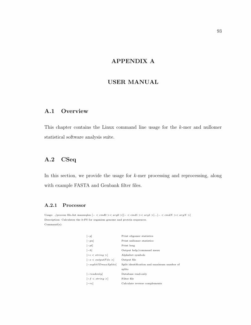
93

APPENDIX A

USER MANUAL

A.1 Overview

This chapter contains the Linux command line usage for the k-mer and nullomer

statistical software analysis suite.

A.2 CSeq

In this section, we provide the usage for k-mer processing and reprocessing, along

with example FASTA and Genbank filter files.

A.2.1 Processor

Usage: ./process file list maxseqlen [− < cmd0 >< arg0 >][− < cmd1 >< arg1 >]...[− < cmdN >< argN >]

Description: Calculates the k-FS for organism genome and protein sequences.

Command(s):

[−p] Print oligomer statistics

[−pn] Print nullomer statistics

[−pl] Print long

[−h] Output help/command menu

[−c < string >] Alphabet symbols

[−o < outputFile >] Output file

[−ssplitIDmaxSplits] Split identification and maximum number of

splits

[−readonly] Database read-only

[−f < string >] Filter file

[−rc] Calculate reverse complements

94

A.2.2 Reprocessor

Usage: ./reprocess file list seqlen [− < cmd0 >< arg0 >][− < cmd1 >< arg1 >]...[− < cmdN >< argN >]

Description: Calculates the (previously processed) k-FS for organism genome and protein sequences as a post-processing utility.

Command(s):

[−jp] Just print.

[−p] Print oligomer statistics

[−pn] Print nullomer statistics

[−o < outputFile >] Output file

[−ssplitIDmaxSplits] Split identification and maximum number of

splits

[−rc] Calculate reverse complements

[−h] Output help/command menu

A.2.3 FASTA Filtering

An example of a CSeq FASTA record filter file which requires the human regular expression to logically exist:

fasta filter:

exist=yes

value=(.)*[Hh]omo [Ss]apien(.)*

An example of a CSeq FASTA record filtering file which requires the chicken regular expression to logically not exist and additionally

the cattle regular expression to not exist:

fasta filter:

exist=no

value=(.)*[Gg]allus [Gg]allus(.)*

AND

fasta filter:

exist=no

value=(.)*[Bb]os [Tt]aurus(.)*

A.2.4 Genbank Filtering

An example of a CSeq Genbank record regular expression filter file which requires the polar bear to logically exist OR the tiger regular

expression to logically not exist at the depth-1 meta-data component (using key/integer-valued parameters):

genbank filter:

input mode=key

filter type=regex

exist=yes

value=(.)*[Pp]olar [Bb]ear(.)*

depth1 attribute=6

depth2 field=0

depth3 subfield=0

OR

genbank filter:

input mode=key

filter type=regex

exist=no

value=(.)*[Tt]iger(.)*

depth1 attribute=6

depth2 field=0

95

depth3 subfield=0

An example of a CSeq Genbank record regular expression filter file which requires the cds (coding region specifier) to logically

exist at the depth-2 meta-data component (using string-valued parameters):

genbank filter:

input mode=string

filter type=region

exist=yes

value=(.)*[Tt]iger(.)*

depth1 attribute=features

depth2 field=cds

depth3 subfield=NULL

An example of a CSeq Genbank record region-specific filter file which screens for the non-cds region (using string-valued parame-

ters):

genbank filter:

input mode=string

filter type=region

exist=no

region=cds

An example of a CSeq Genbank record region-specific filter file which logically screens for the cds AND promoter regions (using

string-valued parameters):

genbank filter:

input mode=string

filter type=region

exist=yes

region=cds

AND

genbank filter:

input mode=string

filter type=region

exist=yes

region=promoter

An example of a CSeq Genbank record region-specific filter file which logically screens for the cds OR promoter regions (using

string-valued parameters):

genbank filter:

input mode=string

filter type=region

exist=yes

region=cds

OR

genbank filter:

input mode=string

filter type=region

exist=yes

region=promoter

96

A.3 Analysis Applications

In this section, we provide the usage for utilities designated for the post-processing stage of the k-mer and prime/nullomer analysis.

A.3.1 Rankseq

Usage: ./rankseq [− < cmd0 >< arg0 >][− < cmd1 >< arg1 >]...[− < cmdN >< argN >]

Description: Calculates the transitional probabilities associated with each sequence motif with respect to the underlying subsequence

probabilities

Command(s):

[−single < sequence >]|[−multiple < filename >] Required: Single sequence or multiple se-

quences listed in a file of specified name

[−statfiles < filename >] Required: Name of file containing the list of

CSeq frequency statistics filenames

[−alphabet < dna|protein >] Required: Specifies the alphabet as ”DNA”

or ”protein”

[−partition < integer >] Required: Maximum subsequence length to

partition the sequence motifs by

[−h] Optional: Print help information

A.3.2 NcbiStat

Usage: ./ncbistat [− < cmd0 >< arg0 >][− < cmd1 >< arg1 >]

Description: Calculates the total sequence length of the supplied NCBI data set in symbols (DNA or protein characters)

Command(s):

[−input < filename >] Required: Name of the file containing a list

of NCBI files

[−filter < filename >] Optional: Name of the filter file


A.3.3 Genseq

Usage: ./genseq [− < cmd0 >< arg0 >][− < cmd1 >< arg1 >]...[− < cmdN >< argN >]

Description: Generates an alphabet-specific sequence of particular size using either (1) CSeqStat frequency statistics or (2) randomly.

Command(s):

97

[−randgen]|[−statgen] Required: Generation mode, specify random

or statistical generation mode

[−statistics < filename >] Required: Name of the file which contains

the list binary statistics frequency files

[−qlen < integer >] Required: Length of string to query for fre-

quency statistics

[−slen < integer >] Required: Maximum sequence processing

length


or ”protein”

[−size < integer >] Required: Size (in symbols) of data set to

generate

[−seed < integer >] Optional: Set the pseudo-random seed value

[−p] Optional: Causes program to print results to

screen

[−pn] Optional: Causes program to print nulls to

screen

[−o < filename >] Optional: Set the name of the output file.

If not specified results will be written to the

screen

[−s < splitID >< maxSplits >] Optional: The number of splits, and splitID

is the split that this instantiation of the pro-

gram will gather stats on

[−rc] Optional: Reprocess binary statistics files

for reverse complements


A.3.4 Freqseq

Usage: ./freqseq [− < cmd0 >< arg0 >][− < cmd1 >< arg1 >]...[− < cmdN >< argN >]

Description: Expresses the relative frequency of a specific sequence length as a function of the exact count, such that the 0 <=

count <= max by generating the corresponding histogram.

Command(s):

[−maxcount < integer >] Required: The maximum exact count

[−slength < integer >] Required: The maximum sequence motif

length

[−statfiles < filename >] Required: Name of the file which contains

the list binary frequency statistic files


or ”protein”

[−n < integer >] Optional: Number of histogram bins (De-

fault: 10 bins)

[−normalize] Optional: Normalize the histogram to dis-

play relative frequencies

[−statistics] Optional: Calculate and output histogram

bin distribution statistics

[−title < string >] Optional: Name/title of the histogram(s) be-

ing generated, this single word value appears

in the output header


98

A.3.5 Nullcountseq

Usage: ./nullcountseq [− < cmd0 >< arg0 >][− < cmd1 >< arg1 >]...[− < cmdN >< argN >]

Description: Calculates the average size and overlap ratio of nullomer sets identified in stat-generated and randomly-generated with

respect to the real NCBI data set.The results are displayed in an n-by-m matrix comma-delimited format, such that n is the maximum

length of the nullomer sequence set and m is the number of datasets being compared/contrasted

Command(s):


[−input < filename >] Required: Name of file containing a list of

file lists, such that each contains the path of

the nullomer sets

A.3.6 Predictseq

Usage: ./predictseq [− < cmd0 >< arg0 >][− < cmd1 >< arg1 >]...[− < cmdN >< argN >]

Description: Supervised machine learning application used to assess nullomer predictability.

Command(s):

[−i < dataset >] Required: Data set input file used to train,

test, or make a prediction

[−train < ann|svm|nbc >< config file >< target accuracy >< epochs >] Optional: Train system

[−test < ann|svm|nbc >< state file >] Optional: Test system

[−predict < ann|svm|nbc >< state file >] Optional Make a prediction

[−o < output file >] Required: Output directory

[−p < integer >] Required: The (Rankseq) subsequence par-

tition length

[−a < dna|protein >] Required: Alphabet (i.e. ”DNA” or ”pro-

tein”)


Example Predictseq ANN configuration file:

learning rate=0.1

learning momentum=0.2

algorithm=FANN TRAIN QUICKPROP

input size=AUTO

hidden size=4

output size=1

activation function=FANN SIGMOID

A.3.7 Tdataformat

Usage: ./tdataformat [− < cmd0 >< arg0 >][− < cmd1 >< arg1 >]...[− < cmdN >< argN >]

Description: Creates a Predictseq data set from (A) a Rankseq output file and (B) a set of nullomers.

Command(s):

[−i < rankseq file >< nullomer file >] Required: Month A and month B input files

[−o < output file >] Required: Data set output file

[−t < ann|svm|nbc >] Required: Learning algorithm format type

[−b] Optional: Balance flag (over-sample the mi-

nority examples)


99

A.3.8 Tdatamerge

Usage: ./tdatamerge [− < cmd0 >< arg0 >][− < cmd1 >< arg1 >]

Description: Consolidates a list of Tdataformat datasets to a single file for use with Predictseq.

Command(s):

[−i < tdataformat file list >] Required: File containing a list of Tdatafor-

mat filenames to merge.

[−o < filename >] Required: Final data set output file.


A.3.9 34Seq

Usage: ./34seq [− < cmd0 >< arg0 >]

Description: Calculates the number sequences with contiguous nucleotide base pair triplets and quadruplets, given a list of sequences.

Command(s):

[−i < dnasequence file list >] Required: File containing a list of sequences

to process.


A.3.10 Setstat

Usage: ./Setstat [− < cmd0 >< arg0 >]

Description: Calculates the default accuracies and NCBI absent-sequence resubmission errors, given a filename list of nullomer/prime

sets.

Command(s):

[−list < filename >] Required: Required: Filename list of nul-

lomer/prime sets


A.4 Format and Display Applications

In this section, we provide the usage for utilities designated to the the post-ranking stage of the k-mer and prime/nullomer analysis.

A.4.1 Rangestat

Usage: ./rangestat [− < cmd0 >< arg0 >][− < cmd1 >< arg1 >]...[− < cmdN >< argN >]

Description: Determines the lower and upper bounds given a list of Rankseq output ranges.

Command(s):

[−range < filename >] Required: Name of the file containing a list

of Rankseq range output files

[−slength < integer >] Optional: Required only for oligomer-

specific statistics; the maximum sequence

length to query the frequency statistics


A.4.2 Histoseq

Usage: ./histoseq [− < cmd0 >< arg0 >][− < cmd1 >< arg1 >]...[− < cmdN >< argN >]

Description: Generates a histogram or set of histograms in *.csv format, based on the user-supplied Rankseq output file.

Command(s):

100

[−rankseq < filename >] Required: Rankseq output file to generate

the histogram from


ing generated, this single word value appears


[−range < filename >] Optional: File containing a list of Rankseq2

range files, used for global normalization of

the data

[−n < integer >] Optional: Number of histogram bins (De-

fault: 10 bins)

[−automerge] Optional: Automatically merges the his-

tograms by normalizing the bin values



[−statistics] Optional: Calculate and output histogram

bin distribution statistics

[−h] Optional: Print help/usage information

A.4.3 Histoavg

Usage: ./histoavg [− < cmd0 >< arg0 >][− < cmd1 >< arg1 >]...[− < cmdN >< argN >]

Description: Averages a list of uniform-sized histograms and their bin values; consolidating them to a single histogram.

Command(s):

[−input < filename >] Required: Name of file containing the list

of uniform-sized histograms to be aver-

aged/consolidated


ing averaged, this single word value appears





A.4.4 Scriptgen

Usage: ./scriptgen [− < cmd0 >< arg0 >][− < cmd1 >< arg1 >]...[− < cmdN >< argN >]

Description: Generates the scripts for the random analysis experiment based on the parameters in the configuration file.

Command(s):

[−config < filename >] Required: Configuration file


Example Scriptgen configuration file:

experiment title=2011-04-17 protein Apis mellifera complete

executable base directory=/home/nschmidt/Development/cseq/src/

output base directory=/genfs-scratch/nschmidt/entropy analysis/protein/

# [CSEQ]

ncbi file list=/genfs-scratch/nschmidt/entropy analysis/protein/cfg/2011-04-17 protein Apis mellifera.input

ncbi filter=NULL

sequence type=PROTEIN

sequence length=5

# [RANKSEQ]

subsequence partition length=3

# [HISTOSEQ]

101

num histogram bins=50

# [GENSEQ]

generation size=4729600

num dataset instances=30

# [FREQSEQ]

freqseq maximum count=5000

freqseq maximum sequence length=5

freqseq num histogram bins=50

freqseq normalize=yes

102

APPENDIX B

SOURCE CODE SNIPPETS

B.1 OverviewIn this brief chapter we highlight source code snippets that are fundamental to instrumenting the prime probability ranking and

prediction.

B.2 Analysis Applications

103

Figure B.1: Rankseq’s sequence probability ranking algorithm

extern long double rankseq2_calculate_transitional_probabilities(

RANKSEQ_CONFIG* config, RANKSEQ2_ELEMENT* element,

const unsigned short max_plen, boost::shared_ptr<Base_Seq_DB>& stats)

{

long double prob = 0.0, p_temp = 0.0;

unsigned int start = 0, end = max_plen, length = strlen(element->sequence);

string motif(element->sequence), temp = "", chars(stats->util.getBase());

/** If short sequence, evaluate immediately */

if(length < max_plen) { return (long double)(stats->getProbability(motif)); }

/** Initialize probability */

else { prob = 1.0; }

temp = string(motif).substr(start, end - start);

/** Acquire initial probability */

prob *= (long double)stats->getProbability(temp);

++start;

++end;

/** Evaluate each character concatenated to the sequence */

while(end <= length)

{


/** Ignore edge case */

if(!temp.length() || (temp[0] == ’ ’)) { break; }

/** Sum probabilities */

p_temp = 0.0;

for(int x = 0; x < (int)chars.length(); x++)

{

/** Evaluate by concatenating each character in alphabet */

temp.replace(max_plen - 1, 1, 1, chars[x]);

p_temp += (long double)stats->getProbability(temp);

}

/** Compute normalized probability of original string */


p_temp = (long double)stats->getProbability(temp) / p_temp;

/** If legal probability, add to existing probability */

if((p_temp) && (fpclassify(p_temp) == FP_NORMAL)) { prob *= (long double)p_temp; }

++start;

++end;

}

return prob;

}

104

APPENDIX C

DETAILED EXPERIMENTATION PROCEDURES

C.1 OverviewThis chapter reports the detailed preparation and procedure the two k-mer experiments.

C.2 Experiment 1C.2.1 Preparation

First, we select the model organisms of interest and prepare the corresponding configuration files. The Scriptgen utility (described

in Section 3.4.4) is used to instrument this experiment on the GeneSIS cluster and requires that a configuration file for each subject

organism is created by the user; each Scriptgen configuration file contains the following parameters to generate the appropriate cluster

execution scripts:

1. Experiment Title: Name to associate with this particular k-mer analysis experiment (i.e. “20110417 protein Apis mellifera”).

All files pertaining to the experiment (including the GeneSIS cluster command execution scripts and results) are stored in a

sub-directory (of the output base directory) with this label.

2. Executable Base Directory: The absolute pathname of the base directory containing the compiled executables (i.e. “/home/nschmidt/Development/cseq/src/”)

3. Output Base Directory: The absolute pathname of the base directory to export the experimentrelated files to (i.e.

“/home/nschmidt/kmer analysis/protein/”).

4. NCBI File List: A file containing the list of NCBI input files to process (i.e. “/home/nschmidt/kmer analysis/protein/2011-

0417 Apis mellifera.input”) with CSeq. In this case since we are interested in specific organisms, the most efficient method

is to create a list file which contains only the Genbank files corresponding to the subject organism (yet recall that it is also

possible to filter for organism-specific entries).

5. NCBI Filter: A file containing NCBI-specific filtering parameters (i.e. “NULL” for no filtering or “/home/nschmidt/kmer analysis/protein/coding region.filter”

for filtering).

6. Sequence Type: The alphabet being processed (i.e. “PROTEIN” or “DNA”). NCBI input files that do not match this

description are automatically discarded by CSeq and related software.

7. Sequence Length: The maximum sequence length that CSeq and related software will process (i.e. “6” or “14”).

8. Sub-sequence Partitioning Length: The maximum partitioning length that Rankseq will process and Genseq will use to

generate artificial genome sequences with (i.e. “5” or “13”).

9. Number of (Histoseq) Histogram Bins: The number of histogram bins used by Histoseq and Histoavg (i.e. “50” or “200”).

105

10. Generation Size: The length of the artificial genome sequence to generate with Genseq (i.e. “4729600”). This value must

match the length of the real organism genome sequence to be comparable, and must be manually identified using the NcbiStat

utility (see Section 3.3.2) before executing the experiment.

11. Number of Data Set Instances: The number of artificial data set instances that Genseq will generate (i.e. “30”). This

value must be set to acquire a proper distribution of data sets to perform a legitimate sequence analysis.

12. Freqseq Maximum Count: The upper limit for the Freqseq k-mer histogram results (i.e. “5000” or “20000”); the utility

calculates the frequencies from 1 up to this value and maps the distribution to a histogram of specified bin size.

13. Freqseq Maximum Sequence Length: The maximum sequence length (i.e. “5” or “13”). This value must be less than the

minimum nullomer length and have a corresponding count file, thus it must not exceed the sub-sequence partitioning length.

14. Number of (Freqseq) Histogram Bins: The number of histogram bins used by Freqseq (i.e. “50”).

15. Freqseq Normalize: The Freqseq histogram normalization flag (i.e. “yes” or “no’).

For an example of this particular file and Scriptgen usage see Section A.4.4.

C.2.2 Procedure

Recall that the GeneSIS cluster command scripts required to execute this experiment are automatically generated by the Scriptgen

utility; however the parameters and options necessary to conduct this particular experiment manually are listed by the user.

Step 1: Process Organism-Specific NCBI Data

Supply the parameters discussed in this section to the CSeq executable “./process”. First, determine the subset of the NCBI database

associated with the organism and create a file consisting of a list of genome input files. If filtering is required, define the filters by

creating the appropriate filter file and specify it using the “-f” option. Determine the alphabet type associated with the organism

(DNA or AA) using the “-a” option and select the nullomer print option “-pn”. Subsequently, choose a maximum target sequence

processing length; let this value be n. Next define the preferred output directory using the “-o” option, and redirect the nullomer

output accordingly.

Step 2: Reprocess Organism-Specific NCBI Data

Supply the parameters discussed in this section to the CSeq executable “./reprocess”. Given the maximum sequence processing length

n, the “./reprocess” must be executed for all sub-subsequence processing lengths ranging from 1 to n− 1. Subsequently we create a file

consisting the file path to the CSeq frequency output file and supply that as an argument. Next, we select the nullomer print option

“-pn” and define the preferred output directory using the “-o” option, and redirect the nullomer output accordingly.

Step 3: Generate and Process Statistically-Biased Artificial Genome Data

Supply the parameters discussed in this section to the Genseq executable “./genseq”. Create a file containing a list of file paths

corresponding to the CSeq frequency output using the “-statistics” option and choose the related “-statgen” option. Given the maximum

sequence processing length n, the “./genseq” must be executed for all sub-subsequence processing lengths ranging from 1 to n− 1 using

the “-slen” option. For each of those, the “./genseq” must be also executed for all sub-subsequence processing lengths ranging from 1

to n − 1 using the “-qlen” option. Determine the alphabet type associated with the organism using the “-a” option and additionally

select the nullomer print option “-pn”. Specify the size of the data set to generate using the “-size” option. Next define the preferred

output directory using the “-o” option, and redirect the nullomer output accordingly.

106

Step 4: Reprocess Statistically-Biased Artificial Genome Data


n, the “./reprocess” must be executed for all sub-subsequence processing lengths ranging from 1 to n− 1 and for each of those because

we previously generated data sets based on specific frequency statistics lengths. Subsequently, we create a file consisting the file path

to the CSeq frequency output file and supply that as an argument. Next we select the nullomer print option “-pn” and define the

preferred output directory using the “-o” option, and redirect the nullomer output accordingly.

Generate and Process Random (Non-Biased) Artificial Genome Data

Supply the parameters discussed in this section to the Genseq executable “./genseq”. Given the maximum sequence processing length

n, the “./genseq” must be executed for all sub-subsequence processing lengths ranging from 1 to n − 1 using the “-slen” option. Next

include the “-randgen” option and determine the alphabet type associated with the organism (DNA or AA) using the “-a protein”

option. Subsequently, supply the reverse complement using the “-rc” option and then select the nullomer print option “-pn”. Specify

the size of the data set to generate using the “-size” option. Next define the preferred output directory using the “-o” option, and

redirect the nullomer output accordingly.

Step 5: Reprocess Random (Non-Biased) Artificial Genome Data


n, the “./reprocess” must be executed for all sub-subsequence processing lengths ranging from 1 to n − 1. If we are analyzing DNA

sequences we must also reprocess for the reverse complement using the “-rc” option and reprocess the range up to n instead of just

n − 1. Subsequently we create a file consisting the file path to the CSeq frequency output file and supply that as an argument. Next

we select the nullomer print option “-pn” and define the preferred output directory using the “-o” option, and redirect the nullomer

output accordingly.

Step 6: Rank the Observed Nullomer Sequences

Supply the parameters discussed in this section to the Rankseq executable “./rankseq”. First, for each data set be sure that a file

containing a list of frequency counts and the length-n nullomers have been created using the “-statfiles” and “-multiple” options,

respectively. Next, supply the alphabet type associated with the organism (DNA or protein) using the “-a protein” option and the

maximum subsequence partitioning length using the “-p” option. Finally, redirect the ranked nullomer output and range boundaries to

standard output and standard error, respectively.

Step 7: Determine the Global Rank Range

Supply the parameters discussed in this section to the Rankseq executable “./rangestat”. First, for each data set create a file containing

a list of Rankseq range boundary files; assign this file as input using the “-range” option. Finally, redirect the global bounds output

accordingly.

Step 8: Construct Comparable Histograms from Nullomer Rankings

Supply the parameters discussed in this section to the Histoseq executable “./histoseq”. First, for each data set specify the Rankseq

and Rangestat output files corresponding to the “-rankseq” and “-range”, respectively. Next, choose a title and specify it using the

“-title” option along with the preferred number of bins via the “-n” option. We recommend using the additional histogram configuration

options “-automerge”, “-normalize”, and “-statistics” flags. Finally, redirect the histogram output accordingly.

107

Step 9: Average the Artificial Genome Histograms for the Nullomers

Supply the parameters discussed in this section to the Histoavg executable “./histoavg”. First, for each data set create a file containing

a list of normalized Histoseq histogram output files and specify it using the “-input” option. Next, choose a title and specify it using

the “-title” option along with the “-normalize” flag. Finally, redirect the consolidated/averaged histogram output accordingly.

Step 10: Identify the Nullomer Set Cardinalities and Intersections

Supply the parameters discussed in this section to the Nullcountseq executable “./nullcountseq”. First, for each data set create a file

containing a list of nullomer set files and specify it using the “-input” option. Next, redirect the consolidated/averaged histogram

output accordingly.

Step 11: Calculate the k-mer Frequency Spectras

Supply the parameters discussed in this section to the Freqseq executable “./freqseq”. First, for each data set supply the file containing

a list of k-mer frequency statistics files using the “-statfiles” option, along with the maximum sequence length n using the “-slength”

option. Next, choose a maximum count and specify it with the “-maxcount” option as well as the alphabet via the “-alphabet” option.

Subsequently, choose the number of bins and the title using the respective “-n” and “-title” options and specify the “-normalize” and

“-statistics” flags. Finally, redirect the output accordingly.

Step 12: Average the Artificial Genome Histograms for the Oligomers

Supply the parameters discussed in this section to the Histoavg executable “./histoavg”. First, for each data set create a file containing

a list of normalized Freqseq histogram output files and specify it using the “-input” option. Next, choose a title and specify it using

the “-title” option along with the “-normalize” flag. Finally, redirect the consolidated/averaged histogram output accordingly.

C.3 Experiment 2C.3.1 Preparation

First, we select the most recent 18 months of NCBI DNA genome snapshots on GeneSIS and create the necessary input and output

files/directories. This experiment does not require a script generator utility and therefore all the command files are created manually

by the user.

Subsequently, Predictseq must be configured prior to the training process– for ANN mode, this is achieved by creating an ANN

configuration file to reflect the user’s preference. The ANN configuration file must contain the following parameters:

1. Learning Rate: The rate at which to adjust the neuron interconnections during training (i.e. “0.1” or “0.7”).

2. Learning Momentum: The learning rate adjustment (i.e. “0.1” or “0.7”).

3. (Training) Algorithm: The supervised machine learning algorithm used to train the network (i.e. “FANN TRAIN QUICKPROP”).

4. Input (Layer) Size: The number of input layer neurons in the network. We recommend the value “AUTO”, which

automatically detects the required number of inputs for the particular task (Rankseq sub-sequence partition length, alphabet

type, etc.).

5. Hidden (Layer) Size: The number of hidden layer neurons in the network (i.e. “4”).

6. Output (Layer) Size: The number of output layer neurons in the network (i.e. “1”).

7. Activation Function: The neuron activation function (i.e. “FANN SIGMOID”).

For an example of this particular file and Predictseq usage see Section A.4.4.

108

C.3.2 Procedure

Here we identify the process of assessing prime predictability. In this case, we consider the complete DNA NCBI snapshots A, B, C,

and D where each corresponds to a chronologically-ordered monthly interval; for simplicity of description Predictseq is trained on the

A-B data set, tested on the B-C data set, and used to predict the length n primes for the C-D data set. For this example, let n = 16

and the sub-sequence partitioning length p = 14 (Note: no primes must exist for length p, otherwise the statistics files will contain

blank entries and Rankseq will complain).

Step 1: Process Month A NCBI Database Snapshot

First, CSeq executable “./process” is used to process the month A length-16 statistics. Thus, we execute:

• “./process month A.ncbi files 16 -c actg -o output directory/monthA/s14 -s 1 4 > /dev/null”,

• “./process month A.ncbi files 16 -c actg -o output directory/monthA/s24 -s 2 4 > /dev/null”,

• “./process month A.ncbi files 16 -c actg -o output directory/monthA/s34 -s 3 4 > /dev/null”, and

• “./process month A.ncbi files 16 -c actg -o output directory/monthA/s44 -s 4 4 > /dev/null”.

In this case the “-s” option is used because we are assuming that the computer node does not have enough random access memory

to store the all possible length 16 sequences at once. Next we create a file called “month A.original counts” containing the following

(tabless) four lines:

output directory/monthA/s14 16 1of1.bin




Step 2: Repocess Month A NCBI Database Snapshot

Next, since we are investigating DNA, we need to use the CSeq executable “./reprocess” to consolidate the month A length-16 primes

into a single file. Thus, we execute:

• ./reprocess month A.original counts 16 -pn -rc -c atcg -o output directory/monthA/ > output directory/monthA/nullomers len16 rc.txt.

In this case the “-rc” option is used because we wish to acquire the reverse complemented nullomers for the next step.

Subsequently, we re-use the CSeq executable “./reprocess” to calculate the month A statistics for lengths ranging from 1 to n− 1.

Thus, we execute:

• “./reprocess month A.original counts 1 -pn -c atcg -o output directory/monthA/> output directory/monthA/nullomers len1.txt”,


• ...,


and

• “./reprocess month A.original counts 15 -pn -c atcg -o output directory/monthA/> output directory/monthA/nullomers len15.txt”.

109

Note that for lengths 1 to n−1 we do not calculate the reverse complements, because the Rankseq utility requires the original statistics

files to acquire proper counts for all considered sub-sequence combinations.

Next we create a file named “month A.counts” containing the following (tab-less) sixteen lines:

output directory/monthA/nullomers len1 rc.txt


...



Step 3: Rank the Observed Nullomer Sequences for Month A

Next, we rank the primes using the Rankseq executable “./rankseq” using the command:

• “./rankseq -multiple output directory/monthA/nullomers len16 rc.txt -statfiles month A.counts -p 14 -a protein> output directory/monthA/rankings len16 rc.csv”

At this point we have completed all processing and post-processing required for the month A snapshot.

Step 4: Process Month B NCBI Database Snapshot

Step 1 is performed for month B and the original frequency counts are stored to the file “month B.original counts”.

Step 5: Create Training Data Set for Months A and B

Next, we create the training data set for months A and B using the Tdataformat executable “./tdataformat” with the command:

• “./tdataformat -i output directory/monthA/rankings len16 rc.csv output directory/monthB/nullomers len16 rc.txt -o output directory/AB.dataset

-t ann”.

If we wish to use minority over-sampling to balance the data set, we append the “-b” flag to the above command.

Step 6: Train Predictseq

Next, to train Predictseq on “AB.dataset” we use the “./predictseq” executable with the command:

• “./predictseq -i output directory/AB.dataset -train ann ann.cfg 90 40000 -o output directory/AB.trained ann -p 14 -a DNA”

where “40000” denotes the number of generations, “90” denotes the target accuracy, and “ann.cfg” denotes Predictseq’s ANN configu-

ration file.

Step 7: Reprocess Month B NCBI Database Snapshot

Step 2 is performed for month B. The length 16 reverse complement nullomers are exported to the file “output directory/monthB/nullomers len16 rc.txt”

and the frequency files for month B are stored in the file “month B.counts”.

Step 8: Rank the Observed Nullomer Sequences for Month B

Step 3 is performed for month B and the nullomer rankings are stored to the file “output directory/monthB/rankings len16 rc.csv”.

Step 9: Process Month C NCBI Database Snapshot

Step 1 is performed for month C and the original frequency counts are stored to the file “month C.original counts”.

110

Step 10: Create Testing Data Set for Months B and C

Next, we create the testing data set for months B and C using the Tdataformat executable “./tdataformat” with the command:

• “./tdataformat -i output directory/monthB/rankings len16 rc.csv output directory/monthC/nullomers len16 rc.txt -o output directory/BC.dataset

-t ann”.


Step 11: Test Predictseq

Next, to test Predictseq on “BC.dataset” we use the “./predictseq” executable with the command:

• “./predictseq -i output directory/BC.dataset -test ann output directory/AB.trained ann -o output directory/BC.tested ann -p

14 -a DNA”.

where “ann.cfg” denotes Predictseq’s AB trained ANN state file.

Step 12: Reprocess Month C NCBI Database Snapshot

Step 2 is performed for month C. The length 16 reverse complement nullomers are exported to the file “output directory/monthC/nullomers len16 rc.txt”

and the frequency files for month C are stored in the file “month C.counts”.

Step 13: Rank the Observed Nullomer Sequences for Month C

Step 3 is performed for month C and the nullomer rankings are stored to the file “output directory/monthC/rankings len16 rc.csv”.

Step 14: Process Month D NCBI Database Snapshot

Step 1 is performed for month D and the original frequency counts are stored to the file “month D.original counts”.

Step 15: Create Prediction Data Set for Months C and D

Next, we create the prediction data set for months C and D using the Tdataformat executable “./tdataformat” with the command:

• “./tdataformat -i output directory/monthC/rankings len16 rc.csv output directory/monthD/nullomers len16 rc.txt -o output directory/CD.dataset

-t ann”.


Step 16: Make a Prediction

Next, to predict using Predictseq on the “CD.dataset” we use the “./predictseq” executable with the command:

• “./predictseq -i output directory/CD.dataset -predict ann output directory/AB.trained ann -o output directory/CD.predictions

-p 14 -a DNA”.

where “ann.cfg” denotes Predictseq’s AB trained ANN state file.

111

APPENDIX D

GRAPHICAL RESULTS

D.1 OverviewIn this brief chapter we provide supplementary histogram results related to the experiments of Chapter 4.

D.2 AA k-FS Results: Apis mellifera ExampleFor visual convenience, only the first 10 bins of the 50 bin histograms are displayed because, in all observed cases, the 40 remaining

bin values monotonically decrease close to zero.

Figure D.1: The honey bee’s length-5 AA nullomer ranking histogram for the NCBIdata set

Figure D.2: The honey bee’s length-5 AA nullomer ranking histogram for the length-1statistically generated data set

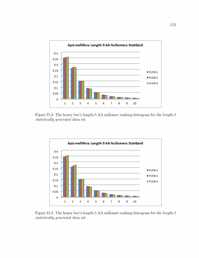
113



114

Figure D.5: The honey bee’s length-5 AA nullomer ranking histogram for therandomly generated data set

on the k-mer frequency spectra of organism genome and

Documents