on the minimum quantum dimension for a given …on the minimum quantum dimension for a given quantum...

On the minimum quantum dimension

for a given quantum correlation

Zhaohui Wei (NTU and CQT, Singapore)

Joint work with Jamie Sikora and Antonios Varvitsiotis

arXiv:1507.00213

We will show a new application of PSD-rank in quantum mechanics


PSD-rank has been shown to be related to quantum information.


PSD-rank has been shown to be related to quantum information. ◦ Communication to compute a function in expectation *1

*1. Fiorini, Massar, Pokutta, Tiwary, de Wolf, J. ACM, 2015.


PSD-rank has been shown to be related to quantum information. ◦ Communication to compute a function in expectation *1

◦ Correlation complexity of distribution *2


*2. Jain, Shi, Wei, Zhang, IEEE T INFORM THEORY, 2013.

An introduction to quantum information

An introduction to device-independent style

The target problem and known results

Our main result and its proof

Applications

Further work and open problems

Quantum state: A positive semidefinite (psd) matrix with the trace

Quantum state: A positive semidefinite (psd) matrix with the trace ◦ Pure state: when is rank 1, i.e., we call pure


◦ Composite systems: . Usually they are huge.



Quantum measurement: A measurement is formed by psd matrices with



Quantum measurement: A measurement is formed by psd matrices with ◦ The outcome is not deterministic:




◦ Measurement will disturb the state





Quantum advantages:





Quantum advantages: ◦ More secure: QKD





Quantum advantages: ◦ More secure: QKD

◦ More efficient: Shor’s algorithm

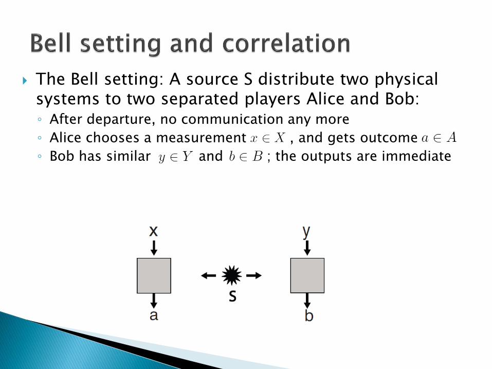
The Bell setting: A source S distribute two physical systems to two separated players Alice and Bob:

The Bell setting: A source S distribute two physical systems to two separated players Alice and Bob: ◦ After departure, no communication any more


◦ Alice chooses a measurement , and gets outcome



◦ Bob has similar and ; the outputs are immediate



◦ Bob has similar and ; the outputs are immediate

◦ After repeating many times, they record the statistics , and we call this a correlation – the correlation between the (classical) inputs and the (classical) outputs

Classical correlation:


Quantum correlation:



A major physical discovery:




The main idea to achieve this: Bell inequality:




The main idea to achieve this: Bell inequality: is a convex polytope, thus described by linear inequalities,

and each of them is called a Bell inequality






◦ For a same scenario, points in can violate some inequality







◦ An example - CHSH inequality: vs.







◦ An example - CHSH inequality: vs.

They can be verified by physical experiments!

Suppose , and . A correlation in this scenario can be expressed as the following block matrix:

Suppose , and . A correlation in this scenario can be expressed as the following block matrix:

with each block being

The difficulties in physical realizations:

The difficulties in physical realizations: ◦ Measurement disturbs states, cannot clone unknown

information: error-correcting is hard, though possible



◦ Quantum states are fragile; memory is short




◦ The accuracy of quantum operations is limited





Quantum control is hard. Especially,





Quantum control is hard. Especially, ◦ The internal working of a quantum device is hard to monitor

Question: Can we know nontrivial internal properties of a quantum system using very limited classical in-out?


Challenge1: The cost to describe a quantum system classically is huge ◦ exponential



Challenge2: One single measurement only reveals very limited information of the system ◦ Typically quantum state collapses



Challenge2: One single measurement only reveals very limited information of the system ◦ Typically quantum state collapses

The answer is YES: the idea of Device-independent (DI)

How to understand?

How to understand? ◦ It is helpful to think the quantum system as a quantum box.

The correctness of DI comes from quantum mechanics, and has nothing to do with how to realize the box specifically



The values of DI:



The values of DI: ◦ Theoretical values on its own




◦ A huge convenience for quantum tasks





Known applications of DI:





Known applications of DI: ◦ quantum key distribution(QKD)

◦ Entropy

◦ Entanglement

Task: Two separated quantum players want to prepare and share a secret classical key

Task: Two separated quantum players want to prepare and share a secret classical key ◦ They have quantum and classical channels, but unsafe


A DI flavor scheme*1:

*1. Artur Ekert, Phys. Rev. Lett, 1991.


A DI flavor scheme*1: ◦ They share a lot of EPR pairs




◦ The choose the following binary POVMs randomly to measure the qubits they have:





Alice





Alice

Bob





Alice

Bob

◦ After all measurements, they announce the choices and outcomes


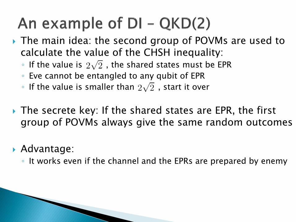
The main idea: the second group of POVMs are used to calculate the value of the CHSH inequality:

The main idea: the second group of POVMs are used to calculate the value of the CHSH inequality: ◦ If the value is , the shared states must be EPR


◦ Eve cannot be entangled to any qubit of EPR



◦ If the value is smaller than , start it over




The secrete key: If the shared states are EPR, the first group of POVMs always give the same random outcomes





Advantage:





Advantage: ◦ It works even if the channel and the EPRs are prepared by enemy






◦ Do not have to check the internal working of quantum devices






◦ Do not have to check the internal working of quantum devices

◦ The base of realistic DI QKD

Question: What is the optimum size of quantum state needed to generate a given quantum correlation?

Question: What is the optimum size of quantum state needed to generate a given quantum correlation? ◦ Size means dimension - a DI style problem


For a given , if there exists a quantum state on , POVMs and s.t.

then admits a d-dimensional representation. We denote by the minimum such d.




For an arbitrarily given , , how to estimate ?




For an arbitrarily given , , how to estimate ? ◦ Dimension is a most fundamental quantum property




For an arbitrarily given , , how to estimate ? ◦ Dimension is a most fundamental quantum property

◦ Dimension is a kind of computational resource

For a fixed Bell scenario, the set of all quantum correlations is convex. However, if restricting dimension, it is usually not.


By allowing free classical correlations, the set of quantum correlations for a given dimension becomes convex:


By allowing free classical correlations, the set of quantum correlations for a given dimension becomes convex: ◦ The setting is changed a little bit



◦ The standard convex analysis method applies



◦ The standard convex analysis method applies

The main known method: dimension witness ◦ Others: entropy method

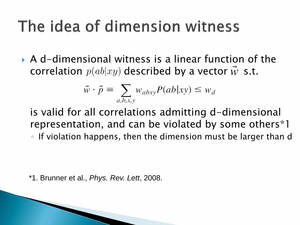
A d-dimensional witness is a linear function of the correlation described by a vector s.t.

is valid for all correlations admitting d-dimensional representation, and can be violated by some others*1

*1. Brunner et al., Phys. Rev. Lett, 2008.


is valid for all correlations admitting d-dimensional representation, and can be violated by some others*1 ◦ If violation happens, then the dimension must be larger than d



is valid for all correlations admitting d-dimensional representation, and can be violated by some others*1 ◦ If violation happens, then the dimension must be larger than d

◦ For different Bell scenarios, the values of ‘s are different


Cannot handle the case without public randomness


Even for the case with classical correlation, it is not a direct function or bound of quantum correlations.



The quantum region for a fixed quantum dimension is very hard to characterize:



The quantum region for a fixed quantum dimension is very hard to characterize: ◦ The values ‘s are hard to compute



The quantum region for a fixed quantum dimension is very hard to characterize: ◦ The values ‘s are hard to compute

◦ Dimension witnesses were found only on some very small quantum systems

We go back to the initial setting, i.e., no free shared randomness is allowed, thus not convex any more.

We go back to the initial setting, i.e., no free shared randomness is allowed, thus not convex any more. ◦ The convex analysis approach fails


◦ The idea of PSD-factorization plays the key role


◦ The idea of PSD-factorization plays the key role

We provide an easy-to-compute lower bound for , which is composed by simple functions of the entries of :

Recall that a correlation is a block matrix:

Let be a nonnegative matrix, then a PSD factorization of size is given by two sets of PSD matrices and satisfying that *1*2

*1. Gouveia, Parrilo, Thomas, Math. Oper. Res., 2013


Let be a nonnegative matrix, then a PSD factorization of size is given by two sets of PSD matrices and satisfying that *1*2

The PSD-rank of , denoted by , is the smallest integer such that has a PSD factorization of size .

*1. Gouveia, Parrilo, Thomas, Math. Oper. Res., 2013


Proof:

Proof: ◦ Suppose it is generated by , and


◦ Purify the state onto with



◦ Set and



◦ Set and

◦ Choose



◦ Set and

◦ Choose

◦ Then

A new characterization for quantum correlations*1

*1. Sikora, Varvitsiotis, 2015.

A new characterization for quantum correlations*1

Thus, is the minimum d to make the above conditions satisfied

*1. Sikora, Varvitsiotis, 2015.

Normalizing the columns of a nonnegative matrix does not change its PSD-rank


Let be a nonnegative matrix with each column summing to 1, if , then there exists a PSD factorization such that

each has trace 1 and all sum to identity*1

*1. Lee, Wei, de Wolf, 2014.


Let be a nonnegative matrix with each column summing to 1, if , then there exists a PSD factorization such that

each has trace 1 and all sum to identity*1 ◦ Each column corresponds the outcome probability distribution

of one quantum state under the same POVM

*1. Lee, Wei, de Wolf, 2014.

Measurement increase the fidelity:

Measurement increase the fidelity:

This is valuable to DI

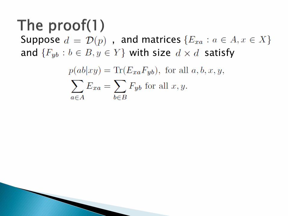
Suppose , and matrices

and with size satisfy



Wlog we let the summation above be full rank, then

there exists an invertible matrix such that



Wlog we let the summation above be full rank, then

there exists an invertible matrix such that

Then for any choice of , is a

valid POVM.

Let , where is a proper

factor such that is a valid quantum state.



Then we have that , which means

for any fixed , is the probability

distribution of the outcome when is measured by

the POVM of .



Then we have that , which means

for any fixed , is the probability

distribution of the outcome when is measured by

the POVM of .

Note that the measurement does not decrease the

fidelity, thus the following is valid for any

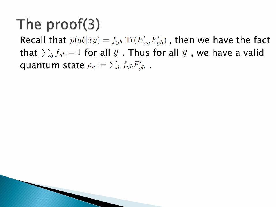
Recall that , then we have the fact

that for all . Thus for all , we have a valid

quantum state .



quantum state .

Note that , then it holds that

. Since is independent in ,

we have that for any , .



quantum state .

Note that , then it holds that

. Since is independent in ,

we have that for any , .

Lastly, note that is a quantum state on , we have

that

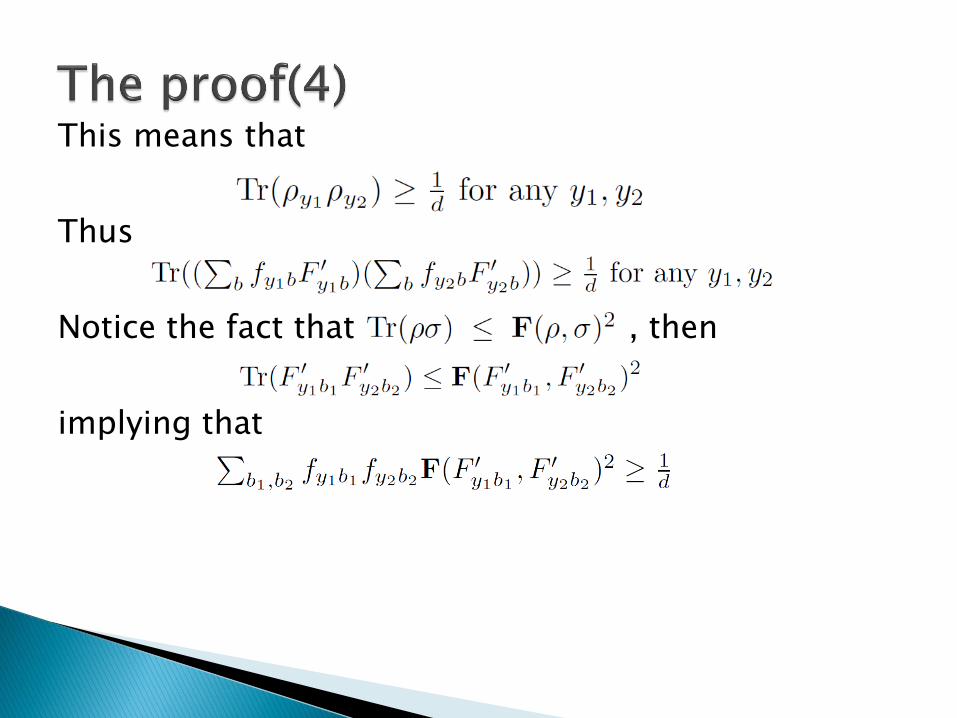
This means that

This means that

Thus

This means that

Thus

Notice the fact that , then

This means that

Thus


implying that

This means that

Thus


implying that

Recall that for any

Combining the last two together, we have that

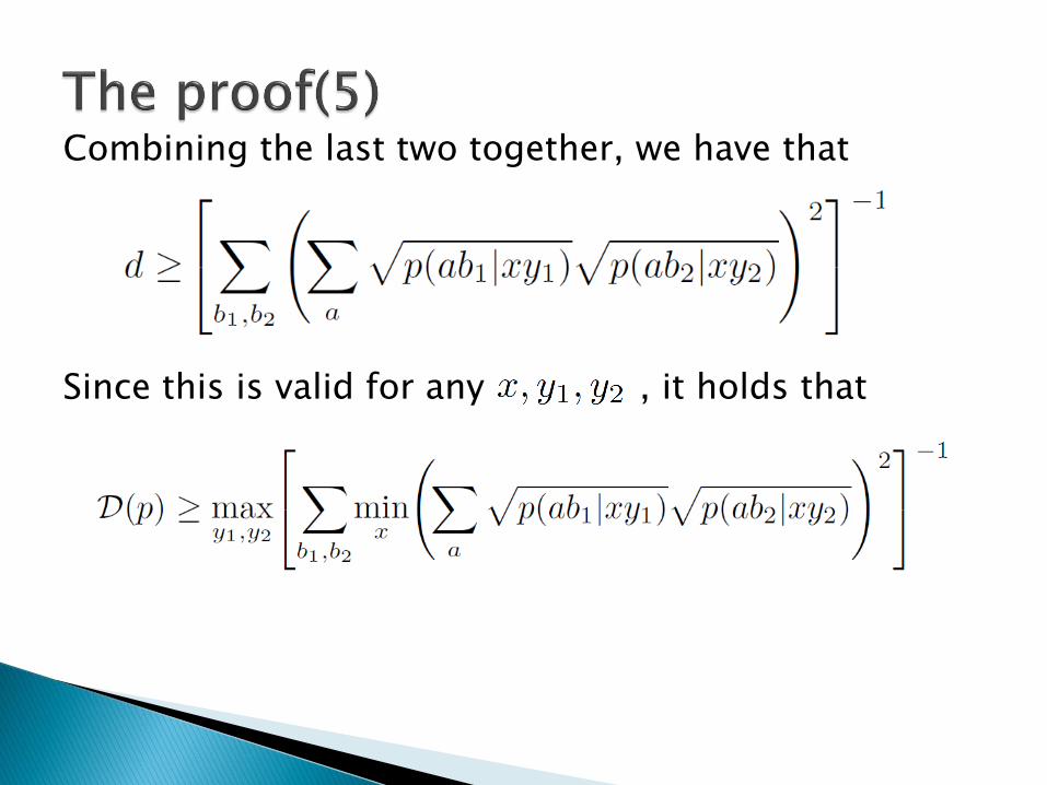
Combining the last two together, we have that

Since this is valid for any , it holds that

If a correlation matrix satisfies the normalization condition, can it always be generated physically?


Answer: no


Answer: no

The correlation cannot violate relativity:


Answer: no

The correlation cannot violate relativity: and are well-defined, i.e., non-signaling

Non-signaling polytope: the set of all correlations that respect the non-signaling rule. A PR-box is a nonlocal vertex of this polytope

Non-signaling polytope: the set of all correlations that respect the non-signaling rule. A PR-box is a nonlocal vertex of this polytope ◦ Question: can it be quantum? No


Set and Then a PR box can be given by


Set and Then a PR box can be given by

The lower bound is infinite, meaning that any finite-dimensional quantum system cannot generate it

A magic square is a Boolean matrix with even row sums and odd column sums


◦ No such a square exists



Consider the following game: Alice and Bob each gets an input corresponding to the index of a row and a column, they are required to give the row and the column themselves, satisfying the above condition (no communication is allowed)

◦ A Bell setting:




◦ A Bell setting:

No classical scheme can win for sure




◦ A Bell setting:


◦ The best winning probability is 8/9




◦ A Bell setting:


◦ The best winning probability is 8/9

Surprisingly, this game can be wined for sure quantumly

◦ Because of stronger correlations quantum provides

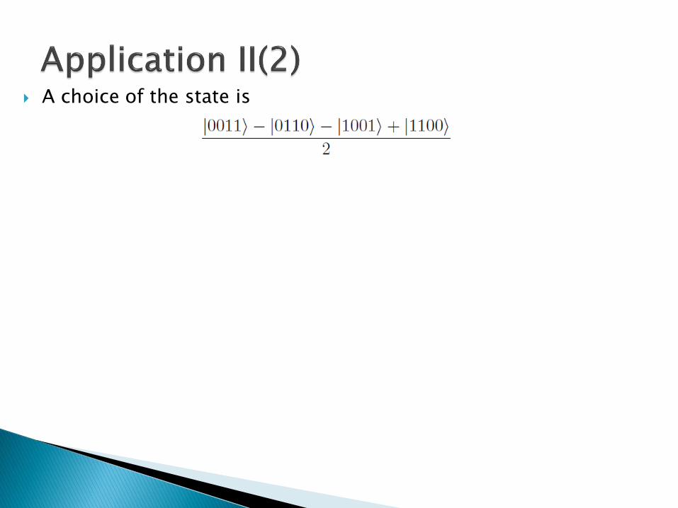
A choice of the state is


and by choosing proper POVMs the correlation can be given as


and by choosing proper POVMs the correlation can be given as

The lower bound is which is tight

If , i.e., each player only has one POVM, the new lower bound goes back to a lower bound for the PSD-rank

If , i.e., each player only has one POVM, the new lower bound goes back to a lower bound for the PSD-rank ◦ Has been given: Lee, Wei, de Wolf, 2014.

This algebraic approach still works:

This algebraic approach still works: ◦ Though classical correlation is free, the combination needs more

than one quantum state

This algebraic approach still works: ◦ Though classical correlation is free, the combination needs more

than one quantum state

Suppose the target quantum correlation is generated by mixing settings with quantum dimensions , then the sum of them is lower bounded by the result

We have given a lower bound for

We have given a lower bound for ◦ The bound is easy to compute


◦ The bound is tight on a lot of famous examples



◦ Composed by simple functions, thus robust to perturbations




How to improve this?




How to improve this? ◦ It can be loose for some cases





Similar lower bound for classical correlations?





Similar lower bound for classical correlations? ◦ The gap will be interesting: one POVM case is known





Similar lower bound for classical correlations? ◦ The gap will be interesting: one POVM case is known

Other physical applications of the PSD-factorization idea? ◦ Works for the prepare-and-measure setting

Thank you

on the minimum quantum dimension for a given …on the minimum quantum dimension for a given quantum...

Documents